Download Combining interval analysis with flatness theory

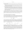
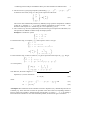
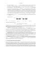
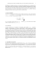
2
Luc Jaulin
(see e.g. [34], [19]). On the other hand, a reliable boat should only enclose reliable sensors. The aim
of this paper is twofold.
• The first goal is to show that the variables that could be measured by the unreliable sensors
could be reconstructed dynamically from the data collected by the reliable sensors. This is new
in a sailboat context, even if the possibility to control a sailboat robot without any wind sensor
has already been demonstrated in [38].
• The second goal is to give a new method which combines nonlinear symbolic observation techniques [9], based on flatness concepts, with interval analysis [31]. The first tool makes it possible to transform the observation problem into equations that have to be solved at each point
of time whereas interval analysis provides a systematic way to solve the inversion problem
[27] taking into account some interval uncertainties on the measured data. Combining interval
analysis with flatness has already been considered for control [16] or source separation [29],
but never for state estimation.
Section 2 shows how the state estimation problem can be transformed into a set inversion
problem parametrized by the time t. Basic notions on interval analysis and the set inversion algorithm
are both presented in Section 3. Section 4 presents the sailboat to be considered and illustrates the
procedure to be followed to transform the state estimation problem into a chain of set inversion
problems. Two simulated testcases are treated on Section 5. Section 6 concludes the paper.
2. Interval flatness approach for state estimation
This section shows how, using flatness theory, a state estimation problem can be cast into a sequence
of set inversion problems that have to be solved at each instant. Shortly speaking, flatness theory can
be seen as a symbolic computation approach to deal easily and efficiently with specific differential
equations. Consider the system described by the following state equations
ẋ
y
= f (x, u)
= g(x),
(2.1)
where u ∈ Rm is the vector of controls (or the vector of actuators), x ∈ Rn is the state vector and
y ∈ Rm is the output vector (or sensors). The functions f and g are the evolution function and the
observation function, respectively. They are assumed to be as smooth as needed. The dimension of
u and that of y are assumed to be both equal to m. All vectors depend on the continuous time t. The
system is said to be flat with the flat output y if there exist two continuous functions φ and ψ and
integers r1 , . . . , rn such that for all t, we have

(rm −1)
 x = φ y1 , ẏ1 , . . . , y (r1 −1) , . . . . . . , ym , ẏm , . . . , ym
1
(2.2)
(rm )
 u = ψ y1 , ẏ1 , . . . , y (r1 ) , . . . . . . , ym , ẏm , . . . , ym
.
1
The integers ri correspond to the relative degrees for the outputs yj , j = 1, . . . , m. According to
Hermann and Krener [18], a system is observable if for any pair of state vector (xa , xb ), xa being
indistinguishable from xb implies xa = xb . Recall that a state vector xa is called indistinguishable
from xb , if for every admissible input u, they produce the same output. Now, from (2.2), two different states cannot produce the same output. We can conclude that all systems satisfying (2.2) are
observable: the function φ gives us the unique state vector which is consistent with the outputs and
their derivatives. Of course, we assume here that the output vector y is measured and that we can
estimate its derivatives with a good accuracy. In practice, the functions φ and ψ involved in (2.2) are
unknown. To get them, we have to proceed in two steps.