Download MAPHYS USER'S GUIDE 0.9.2

M A PH Y S USER ’ S GUIDE 0.9.2
This document explain the Fortran 90 interface of the package M A PH Y S, the
Massively Parallel Hybrid Solver.
Author : HiePaCS Team, INRIA Bordeaux, France
Table des mati`eres
1
General overview
4
2
General introduction
2.1 Parallel hierarchical implementation . . . . . . . . . . . . .
2.2 Dropping strategy to sparsify the preconditioner . . . . . . .
2.3 Sparse approximation based on partial ILU (t, p) . . . . . .
2.4 Exact vs. approximated Schur algorithm to build the precond
.
.
.
.
5
6
9
9
10
3
Installation
3.1 Requirements . . . . . . . . . . . . . . . . . . . . . . . . . . . . . .
3.2 Compilation and installation . . . . . . . . . . . . . . . . . . . . . .
13
13
13
4
Main functionalities of MaPHyS 0.9.2
4.1 Input matrix structure . . . . . . . . . . . . . . . . . . . . . . . . . .
4.2 Arithmetic versions . . . . . . . . . . . . . . . . . . . . . . . . . . .
4.3 The working host processor . . . . . . . . . . . . . . . . . . . . . . .
14
14
14
14
5
Sequence in which routines are called
15
6
Input and output parameters
6.1 Maphys instance . . . . . . . . . . . . . . . . . . .
6.2 Version number . . . . . . . . . . . . . . . . . . . .
6.3 Control of the four main phases . . . . . . . . . . . .
6.4 Control of parallelism . . . . . . . . . . . . . . . . .
6.5 Matrix type . . . . . . . . . . . . . . . . . . . . . .
6.6 Centralized assembled matrix input . . . . . . . . . .
6.6.1 Element matrix input . . . . . . . . . . . . .
6.6.2 Right-hand side and solution vectors/matrices
6.7 Finite element interface(experimental) . . . . . . . .
6.7.1 How to use it . . . . . . . . . . . . . . . . .
6.7.2 Example with finite element interface . . . .
16
16
16
16
16
17
17
17
18
18
18
19
.
.
.
.
.
.
.
.
.
.
.
.
.
.
.
.
.
.
.
.
.
.
.
.
.
.
.
.
.
.
.
.
.
.
.
.
.
.
.
.
.
.
.
.
.
.
.
.
.
.
.
.
.
.
.
.
.
.
.
.
.
.
.
.
.
.
.
.
.
.
.
.
.
.
.
.
.
.
.
.
.
.
.
.
.
.
.
.
.
.
.
.
.
.
.
.
.
.
.
.
.
.
.
.
.
.
.
.
.
.
.
.
.
.
.
7
Writing a matrix to a file
22
8
Using two levels of parallelism inside M A PH Y S
22
9
Control parameters
9.1 ICNTL . . . . . . . . . . . . . . . . . . . . . . . . . . . . . . . . . .
9.2 RCNTL . . . . . . . . . . . . . . . . . . . . . . . . . . . . . . . . .
9.3 Compatibility table . . . . . . . . . . . . . . . . . . . . . . . . . . .
23
23
27
28
2
10 Information parameters
10.1 Information local to each processor . .
10.1.1 IINFO . . . . . . . . . . . . .
10.1.2 RINFO . . . . . . . . . . . .
10.2 Information available on all processes
10.2.1 IINFOG . . . . . . . . . . . .
10.2.2 RINFOG . . . . . . . . . . .
.
.
.
.
.
.
.
.
.
.
.
.
.
.
.
.
.
.
.
.
.
.
.
.
.
.
.
.
.
.
.
.
.
.
.
.
.
.
.
.
.
.
.
.
.
.
.
.
.
.
.
.
.
.
.
.
.
.
.
.
.
.
.
.
.
.
.
.
.
.
.
.
.
.
.
.
.
.
.
.
.
.
.
.
.
.
.
.
.
.
.
.
.
.
.
.
.
.
.
.
.
.
11 Error diagnostics
30
30
30
32
34
34
34
35
12 Examples of use of MaPHyS
12.1 A matrix problem . . . . . . . . . . .
12.1.1 How to write an input file . .
12.1.2 System description . . . . . .
12.1.3 System description . . . . . .
12.2 A cube generation problem . . . . . .
12.3 How to use M A PH Y S in an other code
12.3.1 Fortran example . . . . . . .
12.3.2 C example . . . . . . . . . .
.
.
.
.
.
.
.
.
36
36
36
37
38
38
39
39
42
13 Notes on MaPHyS distribution
13.1 License . . . . . . . . . . . . . . . . . . . . . . . . . . . . . . . . .
13.2 How to refer to M A PH Y S . . . . . . . . . . . . . . . . . . . . . . .
13.3 Authors . . . . . . . . . . . . . . . . . . . . . . . . . . . . . . . . .
45
45
45
45
3
.
.
.
.
.
.
.
.
.
.
.
.
.
.
.
.
.
.
.
.
.
.
.
.
.
.
.
.
.
.
.
.
.
.
.
.
.
.
.
.
.
.
.
.
.
.
.
.
.
.
.
.
.
.
.
.
.
.
.
.
.
.
.
.
.
.
.
.
.
.
.
.
.
.
.
.
.
.
.
.
.
.
.
.
.
.
.
.
.
.
.
.
.
.
.
.
.
.
.
.
.
.
.
.
.
.
.
.
.
.
.
.
.
.
.
.
.
.
.
.
.
.
.
.
.
.
.
.
1
General overview
MaPHyS is a software package for the solution of sparse linear system
Ax = b
where A is a square real or complex non singular general matrix, b is a given righthand-side vector, and x is the solution vector to be computed. It follows a non-overlapping
algebraic domain decomposition method that first reorder the linear system into a 2 × 2
block system
AII AIΓ
xI
bI
=
,
(1)
AΓI AΓΓ
xΓ
bΓ
where AII and AΓΓ respectively represent interior subdomains and separators, and
AIΓ and AΓI are the coupling between interior and separators. By eliminating the
unknowns associated with the interior subdomains AII we get
AII AIΓ
xI
bI
=
,
(2)
0
S
xΓ
f
with
−1
S = AΓΓ − AΓI A−1
II AIΓ and f = bΓ − AΓI AII bI .
(3)
The matrix S is referred to as the Schur complement matrix. Because most of the fillin appears in the Schur complement, the Schur complement system is solved using
a preconditioned Krylov subspace method while the interior subdomain systems are
solved using a sparse direct solver. Although, the Schur complement system is significantly better conditioned than the original matrix A, it is important to consider further
preconditioning when employing a Krylov method.
In MaPHyS, several overlapping block diagonal preconditioning techniques are implemented where each diagonal block is associated with the interface of a subdomain :
1. dense block diagonal factorization : each diagonal block is factorized using the
appropriated LAPACKsubroutine,
2. sparsified block diagonal factorization : the dense diagonal block are first sparsified by droppring entry si,j if it is lower than ξ(|si,i | + |sj,j |). The sparse
factorization is performed by a sparse direct solver.
3. sparse approximation of the diognal block : a sparse approximation of the diagonal block are computing by replacing A−1
II by an approximation computed
using an incomplete ILU (t, p) factorization. Computed approximation of the
Schur complement is further sparsified.
Because of its diagonal nature (consequently local), the preconditioner tends to
be less efficient when the number of subdomains is increased. An efficient solution
using MaPHyS results from a trade-off between the two contradictory ideas that are :
increase the number of domains to reduce the cost of the sparse factorization of the
interior domain and reduce the number of domain to make easier the iterative solution
for the interface solution.
4
2
General introduction
Solving large sparse linear systems Ax = b, where A is a given matrix, b is a given
vector, and x is an unknown vector to be computed, appears often in the inner-most
loops of intensive simulation codes. It is consequently the most time-consuming computation in many large-scale computer simulations in science and engineering, such as
computational incompressible fluid dynamics, structural analysis, wave propagation,
and design of new materials in nanoscience, to name a few. Over the past decade or
so, several teams have been developing innovative numerical algorithms to exploit advanced high performance, large-scale parallel computers to solve these equations efficiently. There are two basic approaches for solving linear systems of equations : direct
methods and iterative methods. Those two large classes of methods have somehow opposite features with respect to their numerical and parallel implementation efficiencies.
Direct methods are based on the Gaussian elimination that is probably among the
oldest method for solving linear systems. Tremendous effort has been devoted to the design of sparse Gaussian eliminations that efficiently exploit the sparsity of the matrices.
These methods indeed aim at exhibiting dense submatrices that can then be processed with computational intensive standard dense linear algebra kernels such as B L AS,
LAPACKand S CA LAPACK. Sparse direct solvers have been for years the methods of
choice for solving linear systems of equations because of their reliable numerical behavior [13]. There are on-going efforts in further improving existing parallel packages.
However, it is admitted that such approaches are intrinsically not scalable in terms of
computational complexity or memory for large problems such as those arising from
the discretization of large 3-dimensional partial differential equations (PDEs). Furthermore, the linear systems involved in the numerical simulation of complex phenomena
result from some modeling and discretization which contains some uncertainties and
approximation errors. Consequently, the highly accurate but costly solution provided
by stable Gaussian eliminations might not be mandatory.
Iterative methods, on the other hand, generate sequences of approximations to the
solution either through fixed point schemes or via search in Krylov subspaces [20].
The best known representatives of these latter numerical techniques are the conjugate
gradient [12] and the GMRES [21] methods. These methods have the advantage that
the memory requirements are small. Also, they tend to be easier to parallelize than
direct methods. However, the main problem with this class of methods is the rate of
convergence, which depends on the properties of the matrix. Very effective techniques
have been designed for classes of problems such as the multigrid methods [10], that are
well suited for specific problems such as those arising from the discretization of elliptic
PDEs. One way to improve the convergence rate of Krylov subspace solver is through
preconditioning and fixed point iteration schemes are often used as preconditioner. In
many computational science areas, highly accurate solutions are not required as long
as the quality of the computed solution can be assessed against measurements or data
uncertainties. In such a framework, the iterative schemes play a central role as they
might be stopped as soon as an accurate enough solution is found. In our work, we
consider stopping criteria based on the backward error analysis [1, 7, 9].
Our approach to high-performance, scalable solution of large sparse linear systems in parallel scientific computing is to combine direct and iterative methods. Such
5
a hybrid approach exploits the advantages of both direct and iterative methods. The
iterative component allows us to use a small amount of memory and provides a natural way for parallelization. The direct part provides its favorable numerical properties.
Furthermore, this combination enables us to exploit naturally several levels of parallelism that logically match the hardware feature of emerging many-core platforms as
stated in Section 1. In particular, we can use parallel multi-threaded sparse direct solvers within the many-core nodes of the machine and message passing among the nodes
to implement the gluing parallel iterative scheme.
The general underlying ideas are not new. They have been used to design domain
decomposition techniques for the numerical solution of PDEs [22, 17, 16]. Domain
decomposition refers to the splitting of the computational domain into sub-domains
with or without overlap. The splitting strategies are generally governed by various
constraints/objectives but the main one is to enhance parallelism. The numerical properties of the PDEs to be solved are usually extensively exploited at the continuous
or discrete levels to design the numerical algorithms. Consequently, the resulting specialized technique will only work for the class of linear systems associated with the
targeted PDEs. In our work, we develop domain decomposition techniques for general
unstructured linear systems. More precisely, we consider numerical techniques based
on a non-overlapping decomposition of the graph associated with the sparse matrices.
The vertex separator, constructed using graph partitioning [14, 5], defines the interface
variables that will be solved iteratively using a Schur complement approach, while the
variables associated with the interior sub-graphs will be handled by a sparse direct solver. Although the Schur complement system is usually more tractable than the original
problem by an iterative technique, preconditioning treatment is still required. For that
purpose, we developed parallel preconditioners and designed a hierarchical parallel implementation. Linear systems with a few tens of millions unknowns have been solved
on a few thousand of processors using our designed software.
2.1
Parallel hierarchical implementation
In this section, methods based on non-overlapping regions are described. Such domain decomposition algorithms are often referred to as substructuring schemes. This
terminology comes from the structural mechanics discipline where non-overlapping
ideas were first developed. The structural analysis finite element community has been
heavily involved in the design and development of these techniques. Not only is their
definition fairly natural in a finite element framework but their implementation can
preserve data structures and concepts already present in large engineering software packages.
Let us now further describe this technique and let Ax = b be the linear problem.
For the sake of simplicity, we assume that A is symmetric in pattern and we denote
G = {V, E} the adjacency graph associated with A. In this graph, each vertex is
associated with a row or column of the matrix A and it exists an edge between the
vertices i and j if the entry ai,j is non zero.
We assume that the graph G is partitioned into N non-overlapping sub-graphs G1 ,
..., GN with boundaries Γ1 , ...., ΓN . The governing idea behind substructuring or Schur
complement methods is to split the unknowns in two subsets. This induces the follo6
wing block reordered linear system :
AII AIΓ
xI
bI
=
,
AΓI AΓΓ
xΓ
bΓ
(4)
where xΓ contains all unknowns associated with sub-graph interfaces and xI contains
the remaining unknowns associated with sub-graph interiors. Because the interior points
are only connected to either interior points in the same sub-graph or with points on the
boundary of the sub-graphs, the matrix AII has a block diagonal structure, where each
diagonal block corresponds to one sub-graph. Eliminating xI from the second block
row of Equation (4) leads to the reduced system
SxΓ = f,
(5)
−1
S = AΓΓ − AΓI A−1
II AIΓ and f = bΓ − AΓI AII bI .
(6)
where
The matrix S is referred to as the Schur complement matrix. This reformulation leads
to a general strategy for solving Equation (4). Specifically, an iterative method can be
applied to Equation (5). Once xΓ is known, xI can be computed with one additional
solve on the sub-graph interiors.
Let Γ denote the entire interface defined by
T Γ = ∪ Γi ; we notice that if two subgraphs Gi and Gj share an interface then Γi Γj 6= ∅. As interior unknowns are no
longer considered, new restriction operators must be defined as follows. Let RΓi :
Γ → Γi be the canonical point-wise restriction which maps full vectors defined on Γ
into vectors defined on Γi . Thus, in the case of many sub-graphs, the fully assembled
global Schur S is obtained by summing the contributions over the sub-graphs. The
global Schur complement matrix, Equation (6), can be written as the sum of elementary
matrices
N
X
S=
RTΓi Si RΓi ,
(7)
i=1
where
Si = AΓi Γi − AΓi Ii A−1
Ii Ii AIi Γi
(8)
is a local Schur complement associated with Gi and is in general a dense matrix (eg :
if AII is irreducible, Si is dense). It can be defined in terms of sub-matrices from the
local matrix Ai defined by
AIi Ii AIi Γi
Ai =
.
(9)
AΓi Ii AΓi Γi
While the Schur complement system is significantly better conditioned than the
original matrix A, it is important to consider further preconditioning when employing
a Krylov method. It is well-known, for example, that κ(A) = O(h−2 ) when A corresponds to a standard discretization (e.g. piecewise linear finite elements) of the Laplace
operator on a mesh with spacing h between the grid points. Using two non-overlapping
7
sub-graphs effectively reduces the condition number of the Schur complement matrix to κ(S) = O(h−1 ). While improved, preconditioning can significantly lower this
condition number further.
We introduce the general form of the preconditioner considered in this work. The
preconditioner presented below was originally proposed in [4] in two dimensions and
successfully applied to large three dimensional problems and real life applications in [8,
11]. To describe this preconditioner we define the local assembled Schur complement,
S¯i = RΓi SRTΓi , that corresponds to the restriction of the Schur complement to the
interface Γi . This local assembled preconditioner can be built from the local Schur
complements Si by assembling their diagonal blocks.
With these notations the preconditioner reads
Md =
N
X
RTΓi S¯i−1 RΓi .
(10)
i=1
If we considered a planar graph partitioned into horizontal strips (1D decomposition), the resulting Schur complement matrix has a block tridiagonal structure as depicted in Equation (11)


..
.




Sk,k
Sk,k+1


.

Sk+1,k Sk+1,k+1 Sk+1,k+2
(11)
S=



S
S
k+1,k+2
k+2,k+2


..
.
For that particular structure of S the submatrices in boxes correspond to the S¯i .
Such diagonal blocks, that overlap, are similar to the classical block overlap of the
Schwarz method when written in a matrix form for 1D decomposition. Similar ideas
have been developed in a pure algebraic context in earlier papers [3, 18] for the solution
of general sparse linear systems. Because of this link, the preconditioner defined by
Equation (10) is referred to as algebraic additive Schwarz for the Schur complement.
One advantage of using the assembled local Schur complements instead of the local
Schur complements (like in the Neumann-Neumann [2, 6]) is that in the SPD case the
assembled Schur complements cannot be singular (as S is SPD [4]).
The original idea of non-overlapping domain decomposition method consists into
subdividing the graph into sub-graphs that are individually mapped to one processor.
With this data distribution, each processor Pi can concurrently partially factorize it
to compute its local Schur complement Si . This is the first computational phase that
is performed concurrently and independently by all the processors. The second step
corresponds to the construction of the preconditioner. Each processor communicates
with its neighbors (in the graph partitioning sense) to assemble its local Schur complement S¯i and performs its factorization. This step only requires a few point-to-point
communications. Finally, the last step is the iterative solution of the interface problem,
Equation ( 5). For that purpose, parallel matrix-vector product involving S, the preconditioner M? and dot-product calculation must be performed. For the matrix-vector
8
product each processor Pi performs its local matrix-vector product involving its local
Schur complement and communicates with its neighbors to assemble the computed
vector to comply with Equation (7). Because the preconditioner, Equation (10), has a
similar form as the Schur complement, Equation (7), its parallel application to a vector
is implemented similarly. Finally, the dot products are performed as follows : each processor Pi performs its local dot-product and a global reduction is used to assemble the
result. In this way, the hybrid implementation can be summarized by the above main
three phases.
2.2
Dropping strategy to sparsify the preconditioner
The construction of the proposed local preconditioners can be computationally expensive because the dense matrices Si should be factorized. We intend to reduce the
storage and the computational cost to form and apply the preconditioner by using sparse
approximation of S¯i in Md following the strategy described by Equation (12). The approximation Sˆi can be constructed by dropping the elements of S¯i that are smaller than
a given threshold. More precisely, the following symmetric dropping formula can be
applied :
0,
if |¯
s`j | ≤ ξ(|¯
s`` | + |¯
sjj |),
˜s`j =
(12)
s¯`j , otherwise,
where s¯`j denotes the entries of S¯i . The resulting preconditioner based on these sparse
approximations reads
Msp =
N
X
−1
˜
RTΓi S
RΓi .
i
(13)
i=1
We notice that such a dropping strategy preserves the symmetry in the symmetric case
but it requires to first assemble S¯i before sparsifying it.
Note : see ICNTL(21)=2 or 3 and RCNTL(11) for more details on how to control
this dropping strategy
Sparse approximation based on partial ILU (t, p)
2.3
One can design a computationally and memory cheaper alternative to approximate
the local Schur complements S (i) . Among the possibilities, we consider in this report
a variant based on the ILU (t, p) [19] that is also implemented in pARMS [15].
The approach consists in applying a partial incomplete factorisation to the matrix
A(i) . The incomplete factorisation is only run on Aii and it computes its ILU factors
˜ i and U
˜i using to the dropping parameter threshold tf actor .
L
pILU (A(i) ) ≡ pILU
Aii
AΓi i
AiΓi
(i)
AΓi Γi
≡
˜i
L
˜ −1
AΓi U
i
where
(i)
˜ −1 L
˜ −1 AiΓ
S˜(i) = AΓi Γi − AΓi i U
i
i
i
9
0
I
˜i
U
0
˜ −1 AiΓ
L
i
S˜(i)
The incomplete factors are then used to compute an approximation of the local
Schur complement. Because our main objective is to get an approximation of the local
Schur complement we switch to another less stringent threshold parameter tSchur to
compute the sparse approximation of the local Schur complement.
Such a calculation can be performed using a IKJ-variant of the Gaussian elimina˜ factor is computed but not stored as we are only interested in an
tion [20], where the L
approximation of S˜i . This further alleviate the memory cost.
Contrary to Equation (13) (see Section 2.2), the assembly step can only be performed after the sparsification, which directly results from the ILU process. as a consequence, the assembly step is performed on sparse data structures thanks to a few neigh(i)
bour to neighbour communications to form S˜ from S˜(i) . The preconditionner finally
reads :
N
X
(i) −1
Msp =
RΓTi S˜
RΓi .
(14)
i=1
Note : To use this method, you should put ICNTL(30)=2, the control parameters
related to the ILUT method are : ICNTL(8), ICNTL(9), RCNTL(8) and RCNTL(9).
2.4
Exact vs. approximated Schur algorithm to build the precond
In a full MPI implementation, the domain decomposition strategy is followed to
assign each local PDE problem (sub-domain) to one MPi process that works independently of other processes and exchange data using message passing. In that computational framework, the implementation of the algorithms based on preconditioners built
from the exact or approximated local Schur complement only differ in the preliminary
phases. The parallel SPMD algorithm is as follow :
1. Initialization phase :
— Exact Schur : using the sparse direct solver, we compute at once the LU
factorization of Aii and the local Schur complement S (i) using A(i) as input
matrix ;
— Approximated Schur : using the sparse direct solver we only compute the
LU factorization of Aii , then we compute the approximation of the local
Schur complement S˜(i) by performing a partial ILU factorization of A(i) .
2. Set-up of the preconditioner :
— Exact Schur : we first assemble the diagonal problem thanks to few neighbour to neighbour communications (computation of S¯(i) ), we sparsify the
assembled local Schur (i.e., Sˆ(i) ) that is then factorized.
— Approximated Schur : we assemble the sparse approximation also thanks to
few neighbour to neighbour communications and we factorize the resulting
sparse approximation of the assembled local Schur.
3. Krylov subspace iteration : the same numerical kernels are used. The only difference is the sparse factors that are considered in the preconditioning step dependent on the selected strategy (exact v.s. approximated).
10
From a high performance computing point of view, the main difference relies in
the computation of the local Schur complement. In the exact situation, this calculation is performed using sparse direct techniques which make intensive use of BLAS-3
technology as most of the data structure and computation schedule are performed in
a symbolic analysis phase when fill-in is analyzed. For partial incomplete factorization, because fill-in entries might be dropped depending on their numerical values, no
prescription of the structure of the pattern of the factors can be symbolically computed. Consequently this calculation is mainly based on sparse BLAS-1 operations that
are much less favorable to an efficient use of the memory hierarchy and therefore less
effective in terms of their floating point operation rate. In short, the second case leads
to fewer operations but at a lower computing rate, which might result in higher overall elapsed time in some situations. Nevertheless, in all cases the approximated Schur
approach consumes much less memory as illustrated later on in this report.
Note : To choose between each strategy you should use ICNTL(30).
R´ef´erences
[1] R. Barrett, M. Berry, T. F. Chan, J. Demmel, J. Donato, J. Dongarra, V. Eijkhout,
R. Pozo, C. Romine, and H. Van der Vorst. Templates for the Solution of Linear
Systems : Building Blocks for Iterative Methods. SIAM, Philadelphia, PA, second
edition, 1994.
[2] J.-F. Bourgat, R. Glowinski, P. Le Tallec, and M. Vidrascu. Variational formulation and algorithm for trace operator in domain decomposition calculations. In
Tony Chan, Roland Glowinski, Jacques P´eriaux, and Olof Widlund, editors, Domain Decomposition Methods, pages 3–16, Philadelphia, PA, 1989. SIAM.
[3] X.-C. Cai and Y. Saad. Overlapping domain decomposition algorithms for general
sparse matrices. Numerical Linear Algebra with Applications, 3 :221–237, 1996.
[4] L. M. Carvalho, L. Giraud, and G. Meurant. Local preconditioners for two-level
non-overlapping domain decomposition methods. Numerical Linear Algebra with
Applications, 8(4) :207–227, 2001.
[5] C. Chevalier and F. Pellegrini. PT-SCOTCH : a tool for efficient parallel graph
ordering. Parallel Computing, 34(6-8), 2008.
[6] Y.-H. De Roeck and P. Le Tallec. Analysis and test of a local domain decomposition preconditioner. In Roland Glowinski, Yuri Kuznetsov, G´erard Meurant,
Jacques P´eriaux, and Olof Widlund, editors, Fourth International Symposium on
Domain Decomposition Methods for Partial Differential Equations, pages 112–
128. SIAM, Philadelphia, PA, 1991.
[7] J. Drkoˇsov´a, M. Rozloˇzn´ık, Z. Strakoˇs, and A. Greenbaum. Numerical stability
of the GMRES method. BIT, 35 :309–330, 1995.
[8] L. Giraud, A. Haidar, and L. T. Watson. Parallel scalability study of hybrid preconditioners in three dimensions. Parallel Computing, 34 :363–379, 2008.
[9] A. Greenbaum. Iterative methods for solving linear systems. Society for Industrial
and Applied Mathematics (SIAM), Philadelphia, PA, 1997.
11
[10] W. Hackbusch. Multigrid methods and applications. Springer, 1985.
[11] A. Haidar. On the parallel scalability of hybrid solvers for large 3D problems.
Ph.D. dissertation, INPT, June 2008. TH/PA/08/57.
[12] M. R. Hestenes and E. Stiefel. Methods of conjugate gradients for solving linear
system. J. Res. Nat. Bur. Stds., B49 :409–436, 1952.
[13] N. J. Higham. Accuracy and Stability of Numerical Algorithms. Society for Industrial and Applied Mathematics, Philadelphia, PA, USA, second edition, 2002.
[14] G. Karypis and V. Kumar. M ETI S – Unstructured Graph Partitioning and Sparse
Matrix Ordering System – Version 2.0. University of Minnesota, June 1995.
[15] Z. Li, Y. Saad, and M. Sosonkina. pARMS : A parallel version of the algebraic
recursive multilevel solver. Technical Report Technical Report UMSI-2001-100,
Minnesota Supercomputer Institute, University of Minnesota, Minneapolis, 2001.
[16] T. Mathew. Domain Decomposition Methods for the Numerical Solution of Partial Differential Equations. Springer Lecture Notes in Computational Science and
Engineering. Springer, 2008.
[17] A. Quarteroni and A. Valli. Domain decomposition methods for partial differential equations. Numerical mathematics and scientific computation. Oxford
science publications, Oxford, 1999.
[18] G. Radicati and Y. Robert. Parallel conjugate gradient-like algorithms for solving
nonsymmetric linear systems on a vector multiprocessor. Parallel Computing,
11 :223–239, 1989.
[19] Y. Saad. ILUT : a dual threshold incomplete ILU factorization. Numerical Linear
Algebra with Applications, 1 :387–402, 1994.
[20] Y. Saad. Iterative Methods for Sparse Linear Systems. SIAM, Philadelphia, 2003.
Second edition.
[21] Y. Saad and M. H. Schultz. GMRES : A generalized minimal residual algorithm
for solving nonsymmetric linear systems. SIAM J. Sci. Stat. Comp., 7 :856–869,
1986.
[22] B. F. Smith, P. Bjørstad, and W. Gropp. Domain Decomposition, Parallel Multilevel Methods for Elliptic Partial Differential Equations. Cambridge University
Press, New York, 1st edition, 1996.
12
3
3.1
Installation
Requirements
M A PH Y S needs some libraries in order to be installed :
— A MPI communication library ( INTEL MPI MPICH2, O PEN MPI, ...) ;
— A B L AS and LAPACK library ( MKL of preference)
— The S COTCH library for the partitioning of the adjacency graph of the sparse
matrix ;
— The MUMPSor PA S TI X library as sparse solver ;
— Optionnally the HWLOC library for a better fit with the hardware topology..
3.2
Compilation and installation
To compile and install M A PH Y S, follow the six following steps :
— Install SCOTCH 5.xx or higher ;
— Install HWLOC ;
— Install MUMPS 4.7 or higher ;
— Uncompress the M A PH Y S archives, copy the file Makefile.inc.example into
Makefile.inc ;
— Set the variable of the Makefile.inc depending of your architecture and library
(such as MPI and B L AS) available ;
— Choose the user’s compiling options : arithmetic (real or complex..), solvers
choice, in the Makefile.inc file ;
— Compile : make all in order to get the library and test program.
13
4
4.1
Main functionalities of MaPHyS 0.9.2
Input matrix structure
In the current version of M A PH Y S, the input matrix can only be supplied centrally
on the host processor (process 0) in elemental format.
For full details, refer to Section 6.6.1 .
4.2
Arithmetic versions
The package is available in the four arithmetics : REAL, DOUBLE PRECISION,
COMPLEX, DOUBLE COMPLEX.
Please refer to the root README of M A PH Y S sources for full details.
4.3
The working host processor
In the current version, the working host process is fixed to the process with MPI
rank 0 according to the chosen communicator (see Section 6.4).
14
5
Sequence in which routines are called
The M A PH Y S package provides one single static library libmaphys.a, which contains
all the artihmetic versions specified in WITH ARITHS (see topdir/Makefile.inc).
The calling sequence of M A PH Y S is similar for all arithmetics, and may look like
this for the DOUBLE PRECISION case :
...
Use DMPH_maphys_mod
Implicit None
Include "mpif.h"
...
Integer :: ierr
Type(DMPH_maphys_t) :: mphs ! one per linear system to solve
...
Call MPI_Init(ierr)
...
mphs%comm = ... ! set communicator
mphs%job = -1
! request initialisation
Call DMPH_maphys_driver(mphs)
...
mphs%sym
= ... ! set matrix input
mphs%n
= ... ! set matrix input
mphs%nnz
= ... ! set matrix input
mphs%rows
= ... ! set matrix input
mphs%cols
= ... ! set matrix input
mphs%values = ... ! set matrix input
mphs%rhs
= ... ! set the right-hand side
...
mphs%icntl(10) = ... ! set the arguments (components of the structure)
mphs%job = 6
! request to perform all steps at once
Call DMPH_maphys_driver(mphs)
...
Call MPI_Finalize(ierr)
To select another arithmetic, simply change the prefix DMPH by CMPH for
the COMPLEX arithmetic ; or SMPH for the REAL arithmetic ; or ZMPH for the
DOUBLE COMPLEX arithmetic.
For convenience purpose, M A PH Y S also generates static libraries specific to one
arithmetic only, namely :
— libcmaphys for the COMPLEX arithmetic ;
— libdmaphys for the DOUBLE PRECISION arithmetic ;
— libsmaphys for the REAL arithmetic ;
— libzmaphys for the DOUBLE COMPLEX arithmetic ;
15
6
6.1
Input and output parameters
Maphys instance
mphs is the structure that will describe one linear system to solve. You have to use
one structure for each linear system to solve.
6.2
Version number
mphs%VERSION (string) gives information about the current M A PH Y S version.
It is set during the intialization step (mphs%JOB=-1)
6.3
Control of the four main phases
The main action performed by M A PH Y S is specified by the integer mphs%JOB.
The user must set it on all processes before each call to M A PH Y S. Possible values of
mphs%JOB are :
— -1 initializes the instance. It must be called before any other call to M A PH Y S.
M A PH Y S will nullify all pointers of the structure, and fill the controls arrays
(mphs%ICNTL and mphs%RCNTL) with default values.
— -2 destroys the instance. M A PH Y S will free its internal memory.
— 1 perfoms the analysis. In this step, M A PH Y S will pretreat the input matrix,
compute how to distribute the global system, and distribute the global system
into local systems.
— 2 performs the factorization assuming the data is distributed in the form of local
systems. In this step, M A PH Y S will factorize the interior of the local matrices,
and compute their local Schur complements.
— 3 performs the preconditioning. In this step, M A PH Y S will compute the preconditioner of the Schur complement system.
— 4 performs the solution. In this step, M A PH Y S will solve the linear system. Namely, M A PH Y S will reformulate the right-hand-side of the input linear system
(mphs%RHS) into local system right-hand-sides, solve the Schur complement
system(s), solve the local sytem
— 5 combines the actions from JOB=1 to JOB=3.
— 6 combines the actions from JOB=1 to JOB=4.
6.4
Control of parallelism
— mphs%COMM (integer) is the MPI communicator used by M A PH Y S. It must
be set to a valid MPI communicator by the user before the initialization step
(mphs%JOB = -1) , and must not changed later. In the current version, the MPI
communicator must have a number of process that is a power of 2.
16
6.5
Matrix type
— mphs%SYM (integer) specifies the input matrix type. It is accessed during the
analysis and the solve steps (mphs%JOB == -1 and mphs%JOB == 4 respectively). M A PH Y S does not modify its value during its execution. Possible values
of mphs%SYM are :
— 0 or SM SYM IsGeneral means the input matrix is General (also known
as Unsymmetric).
— 1 or SM SYM IsSPD means the input matrix is SPD (Symmetric Positive
Definite) in real arithmetics (s/d). In complex arithmetics (z/c), this is an
invalid value.
— 2 or SM SYM IsSymmetric means the input matrix is Symmetric (even in
complex).
In this version, M A PH Y S does not support Hermitian or Hermitian Positive
Definite values.
6.6
Centralized assembled matrix input
There is currently no way to specifies that the matrix is already assembled. Current
version will treat it as an elemental matrix input.
6.6.1
Element matrix input
mphs%SYM, mphs%N, mphs%NNZ, mphs%ROWS, mphs%COLS, mphs%VALUES,
specifies the input matrix in elemental coordinate format. Those components are accessed during the analysis step and the solving step (to compute statistics) by the host
process. They are not altered by maphys.
In details :
— mphs%SYM (integer) specifies the type of symmetry ( see section 6.5 )
— mphs%N (integer) specifies the order of the input matrix. (hence N ¿ 0 )
— mphs%NNZ (integer) specifies the number of the entries in the input matrix.
(hence N N Z > 0 )
— mphs%ROWS (integer array of size NNZ) lists the row indices of the matrix
entries
— mphs%COLS (integer array of size NNZ) lists the column indices of the matrix entries
— mphs%VALUES (Real/Complex array of size NNZ) lists the values of the
matrix entries
Note that, in the case of symmetric matrices(SYM=1 or 2), only half of the matrix
should be provided. For example, only the lower triangular part of the matrix (including the diagonal) or only the upper triangular part of the matrix (including the diagonal) can be provided in ROWS, COLS, and VALUES. More precisely, a diagonal
nonzero A must be provided as A(k) = Aii , ROW S(k) = COLS(k) = i, and a
pair of off-diagonal nonzeros Aij = Aji must be provided either as A(k) = Aij and
ROW S(k) = i, COLS(K) = j or vice-versa. Again duplicates entries are summed.
In particular, this means that if both Aij and Aji are provided, they will be summed.
17
6.6.2
Right-hand side and solution vectors/matrices
— mphs%RHS (Real/Complex array of lenght mphs%N) is the centralized righthand-side of the linear system. It holds the right-hand-side allocated and filled
by the user, on the host, before the solve step (mphs%JOB == 4,6). M A PH Y S
do not alterate its value.
— mphs%SOL (Real/Complex array of lenght mphs%N) is the centralized initial
guess and/or the solution of the linear system. It must be allocated by the user
before the solve step (mphs%JOB == 4,6).
— Before the solve step, on the host, it holds the initial guess if the initial guess
option is activated (mphs%icntl(23) == 1).
— After the solve step, on the host, it holds the solution.
The current version does not support multiple right-hand-sides.
6.7
Finite element interface(experimental)
6.7.1
How to use it
M A PH Y S provides a distributed interface according to finite element interface.
The control of which interface you want to use is define by ICNTL(43). In order to use
the finite element interface the user has to call a routine called xmph create domain
defined as follows before the analysis step :
xmph_create_domain(mphs, myndof, myndofinterior, myndofintrf,
lenindintrf, mysizeintrf,gballintrf, mynbvi,
myindexvi, myptrindexvi, myindexintrf,
myinterface,myndoflogicintrf, mylogicintrf, weight)
The parameters are defined as follow :
— mphs : the M A PH Y S instance
— myndof : integer equal to the degree of freedom of the entire domain (interface
+ interior) ;
— myndof interior : integer equal to the degree of freedom of the domain interior ;
— myndof intrf : integer equal to the degree of freedom of the domain interface ;
— lenindintrf : integer equal to the size of the array myindexintrf
— mysizeintrf : integer equal to the size of the domain interface ;
— gballintrf : integer equal to the total size of each interfaces in each processus ;
— mynbvi : integer equal to the number of neighbor of the processus ;
— myindexV i(:) : list of each neighbors of the domain by rank processus ;
— myptrindexV i(:) : pointer to the first node of the interface of each domain ;
— myindexintrf (:) : list of the node of the domain interface, index are in local
ordering ;
— myinterf ace(:) : conversion from local ordering to global ordering ;
— myndof logicintrf : Integer corresponding to the number of node in the interface wich who the domain is responsable for ;
18
2
10
11
1
7
0
6
2
12
3
3
4
8
9
5
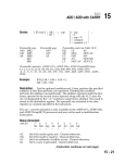
1
F IGURE 1 – The separators are circled in red, the number in bold are the processus id,
the nodes number are in global ordering
— mylogicintrf (:) : list of the nodes that this domain is responsible for (in the
local ordering).
6.7.2
Example with finite element interface
According to this input graph of the matrix already distributed amound processors
as describe in figure 1.
The users will have to call the function with the parameters of xmph create domains
defined as follow for each processus :
19
domain 0 :
domain 1 :
myndof : 7
myndof interior : 2
myndof intrf : 5
myint Lg : 0
lenindintrf : 10
mysizeintrf : 5
gballintrf : 6
mynbvi : 3
myindexV i(:) : 3 2 1
myptrindexV i(:) : 1 3 6 11
myindexintrf (:)
:
4 5 3 4 5 3 4 5 1 2
myinterf ace(:) : 4 5 1 2 3
myndof logicintrf : 5
mylogicintrf (:) : 3 4 5 6 7
myndof : 6
myndof interior : 1
myndof intrf : 5
myint Lg : 0
lenindintrf : 10
mysizeintrf : 5
gballintrf : 6
mynbvi : 3
myindexV i(:) 3 2 0
myptrindexV i(:) : 1 3 6 11
myindexintrf (:)
:
4 5 3 4 5 3 4 5 1 2
myinterf ace(:) : 4 5 1 2 3
myndof logicintrf : 0
mylogicintrf (:) :
domain 2 :
domain 3 :
myndof : 6
myndof interior : 2
myndof intrf : 4
myint Lg : 0
lenindintrf : 9
mysizeintrf : 4
gballintrf : 6
mynbvi : 3
myindexV i(:) : 3 1 0
myptrindexV i(:) : 1 4 7 10
myindexintrf (:)
3 4 1 2 3 4 2 3 4
myinterf ace(:) : 6 1 2 3
myndof logicintrf : 1
mylogicintrf (:) : 3
myndof : 4
myndof interior : 1
myndof intrf : 3
myint Lg : 0
lenindintrf : 7
mysizeintrf : 3
gballintrf : 6
mynbvi : 3
myindexV i(:) : 2 1 0
myptrindexV i(:) : 1 4 6
myindexintrf (:)
2 3 1 2 3 2 3
myinterf ace(:) : 6 2 3
myndof logicintrf : 0
mylogicintrf (:) :
:
8
The local matrices according to this decomposition is described in figure 2.
The user has to describe this matrix and the right hand side as in the centralized
interface, except that the matrix and rhs given will be the local ones and not the global
one.
20
:
glob 7
loc 1
8
Domain 0
4 5 1
2
3
2
3
6
7
4
5
Domain 2
glob 10 11 6 1 2
loc
1 2 3 4 5
glob 9
loc 1
3
4
2
Domain 1
5 1 2
3
4
5
3
6
Domain 3
glob 12 6 2 3
1 2 3 4
loc
6
F IGURE 2 – The different matrices with their local and global orderings. The interface
nodes are in red, the interior nodes are in black
21
7
Writing a matrix to a file
The user may get the preprocessed input matrix (assembled and eventually
symmetrised in structure) by setting the string mphs%WRITE MATRIX (string) on
process 0 before the analysis step (mphs%JOB=1). This matrix will be written during
the analysis step on the file mphs%WRITE MATRIX in matrix market format.
8
Using two levels of parallelism inside M A PH Y S
The current release of M A PH Y S support a two levels of parallelism (MPI +
T HREADS).
In oder to activate the multithreading into M A PH Y S you have to set some control
parameters :
— ICNTL(42) = 1 : Activate the multithreading inside M A PH Y S ;
— ICNTL(37) = The number of nodes ;
— ICNTL(38) = The number of cores on each nodes ;
— ICNTL(39) = The number of MPI process ;
— ICNTL(40) = The number of Threads that you want to use inside each MPI
process.
You can also set ICNTL(36) in order to specify the binding you want to use inside
M A PH Y S as follow :
— 0 = Do not bind ;
— 1 = Thread to core binding ;
— 2 = Grouped bind.
note 1 : Be carreful that if you use more threads than cores available no binding will
be perform.
note 2 : Depending on the problem you want to solve it could be better to use more
MPI process than using threads you can found a study on some problem in the Stojce
Nakov PHD thesis.
22
9
Control parameters
The execution of M A PH Y S can be controlled by the user through the 2 arrays
mphs%ICNTL and mphs%RCNTL. When an execution control should be
expressed as an integer (or an equivalent), this control is a entry of mphs%ICNTL ;
and when an execution control should be expressed as a float (or an equivalent), this
control is a entry of mphs%RCNTL.
9.1
ICNTL
mphs%ICNTL is an integer array of size MAPHYS ICNTL SIZE.
ICNTL(1) Controls where are written error messages. Fortran unit used to write error
messages. Negative value means do not print error messages.
— Default = 0 (stderr)
ICNTL(2) Controls where are written warning messages. Fortran unit used to write
warning messages. Negative value means do not print warning messages.
— Default = 0 (stderr)
ICNTL(3) Controls where are written statistics messages. Fortran unit used to write
statistics messages. Negative value means do not print statistics.
— Default = 6 (stdout)
ICNTL(4) Controls the verbosity of maphys.
— ≤ 0 = do not print output
— 1 = print errors.
— 2 = print errors, warnings & main statistics
— 3 = print errors, warnings & several detailled statistics
— 4 = print errors, warnings & verbose on detailled statistics
— > 4 = debug level
— Default = 3
ICNTL(5) Controls when to print list of controls ( ?cntl). This option is useful to check
if a control is taken into account.
— 0 = never print
— 1 = print once at the begining of analysis
— 2 = print at the begining of each step.
— Default = 0
ICNTL(6) Controls when to print list of informations ( ?info*). This option is useful
while performing benchmarks.
— 0 = never print
— 1 = print once (at the end of solve)
— 2 = print at the end of each step
— Default = 0
ICNTL(7) UNUSED in current version
ICNTL(8) controls the Partial ILUT solver. level of filling for L and U in the ILUT
method. ( that is the maximun number of entries per row in the LU factorization.
23
) This parameter is only relevant while using ILUT and is accessed during factorisation by each process. User must set this parameter while using ILUT before
the factorisation. See also : ICNTL(30), ICNTL(9), RCNTL(8) and RCNTL(9).
Warning : the default value is a bad value.
— Default = -1
Note : For more details on ILU method, you may refer to Section 2.3
ICNTL(9) controls the Partial ILUT solver. level of filling for the Schur complement
in the ILUT method (that is the maximun number of entries per row in the Schur
complement). This parameter is only relevant while using ILUT and is accessed
during factorisation by each process. User must set this parameter while using
ILUT before the factorisation. See also : ICNTL(30),ICNTL(8), RCNTL(8)
and RCNTL(9). Warning : the default value is a bad value.
— Default = -1
Note : For more details on ILU method, you may refer to Section 2.3
ICNTL(10 :12) UNUSED in current version
ICNTL(13) the sparse direct solver package to be used by MAPHYS. It is accessed
during the factorization and the the preconditionning step by each MPI process.
— 1 = use MUMPS
— 2 = use PaSTiX
— 3 = use multiple sparse direct solvers. See ICNTL(15) and ICNTL(32)
— Default = the first available starting from index 1.
ICNTL(14) UNUSED in current version
ICNTL(15) the sparse direct solver package to be used by MAPHYS for the computing the preconditioner. It is accessed during the preconditioning step, by each
MPI process.
— 1 = use MUMPS
— 2 = use PaSTiX
— Default = value of ICNTL(13)
ICNTL(16 :19) UNUSED in current version
ICNTL(20) controls the 3rd party iterative solver used.
— 0 = Unset
— 1 = use Pack GMRES
— 2 = use Pack CG
— 3 = use Pack CG if matrix is SPD, Pack GMRES otherwise
— Default = 3
ICNTL(21) The strategy for preconditionning the Schur. Warning : If (ICNTL(30)=2)
and (ICNTL(21)/=4) then ICNTL(21) must be 3.
— 1 = Preconditioner is the dense factorization of the assembled local schur.
— 2 = Preconditioner is the sparse factorization of the assembled local schur,
you have to specify the threshold using RCNTL(11).
— 3 = Preconditioner is the factorization of a sparse matrix. Where the sparse
matrix is the assembly of the approximated local schur computed with the
Partial Incomplete LU (PILUT), you have to specify the threshold using
RCNTL(9).
24
— 4 = No Preconditioner.
— 5 = autodetect, order of preferences is 1 > 2 > 3 > 4.
— Default = 2
Note : For more details on dropping strategy (ICNTL(21) = 2 or 3), you may
refer to Section 2.2, the parameter RCNTL(8)/RCNTL(9) if ICNTL(21)=2/3 respectivly
ICNTL(22) controls the iterative solver. Determines which orthogonalisation scheme
to apply.
— 0 = modified Gram-Schmidt orthogonalization (MGS)
— 1 = iterative selective modified Gram-Schmidt orthogonalization (IMGS)
— 2 = classical Gram-Schmidt orthogonalization (CGS)
— 3 = iterative classical Gram-Schmidt orthogonalisation (ICGS)
— Default = 3
ICNTL(23) controls the iterative solver. Controls whether the user wishes to supply
an initial guess of solution vector in (mphs%SOL). It must equal to 0 or 1. It is
accessed by all processes during the solve step.
— 0 = No initilization guess (start from null vector)
— 1 = User defined initialization guess
— Default = 0
ICNTL(24) controls the iterative solver. It define the maximumn number of iterations
(cumulated over restarts) allowed. It must be equal or larger than 0 and be the
same on each process.
— 0 = means the parameter is unset, M A PH Y S will performs at most 100
iterations
— > 0 = means the parameter is set, M A PH Y S will performs at most ICNTL(24)
iterations
— Default = 0
ICNTL(25) controls the iterative solver. Controls the strategy to compute the residual
at the restart, it must be the same on each process. It is unrelevant while the
iterative solver is CG (ICNTL(20) = 2,3)
— 0 = A recurrence formula is used to compute the residual at each restart,
except if the convergence was detected using the Arnoldi residual during
the previous restart.
— 1 = The residual is explicitly computed using a matrix vector product
— Default = 0
ICNTL(26) controls the iterative solver, it is the restart parameter of GMRES. Controls
the number of iterations between each restart. It is unrelevant while the iterative
solver is CG (ICNTL(20) = 2,3).
— 0 = means the parameter is unset, M A PH Y S will restart every 100 iterations
— > 0 = means the parameter is set, M A PH Y S will restart every ICNTL(24)
iterations
— Default = 0
ICNTL(27) controls the iterative solver, it is the method used to perform multiplication between the Schur complement matrix and a vector. It should be set
25
before the solving step on each process. It can be set on each process before the
preconditioning step to allow possible memory footprint reduction (peak and
usage).
— -1 = Value unset (error)
— 0 = automatic (1 if possible, 2 if not.)
— 1 = Product of schur complement with a vector is performed explicitly. That
is, the Schur complement is stored in a dense matrix, and a BLAS routine
is called to perform the product.
— 2 = Product of schur complement with a vector is performed implicitly. That
is, we do not use a schur complement stored in a dense matrix, to perform
the product. Indeed, a “solve” and several sparse matrix/vector products
are used to perform the product. This is done by using the definition schur
complement, which is : S = Ai,Γ .A−1
i,i .Ai,Γ − AΓ,Γ This option reduce the
memory footprint by substituing in memory the schur complement by the
preconditioner.
— Default = 0
ICNTL(28) controls the iterative solver. Controls whether you want to use the residual norm on the local rhs or in the global rhs. It must equal to 0 or 1. It is
accessed by all processes during the solve step.
— 0 = Compute the residual on the local right hand side
— 1 = Compute the residual on the global right hand side (only available in
the centralized version (ICNTL(43) = 0)
— Default = 0
ICNTL(29) UNUSED in current version
ICNTL(30) controls how to compute the schur complement matrix or its approximation. It is accessed during the factorisation step by each process. Each processor
must have the same value (current version do not check it). Valid values are :
— 0 = use the schur complement returned by the sparse direct solver package.
— 2 = approximate computation done using a modifyied version of partial
ILUT (PILUT). In this case, user must set ICNTL(8), ICNTL(9), RCNTL(8)
and RCNTL(9) the parameters of PILUT. This option force the preconditioner choice (ICNTL(21) = 3). Note : For more details on ILU method, you
may refer to Section 2.3
— Default = 0
Note : For more details on exact and approximated Schur, you may refer to
Section 2.4
ICNTL(31) UNUSED in current version
ICNTL(32) the sparse direct solver package to be used by MAPHYS for the computing the local schur and perform the local factorisation. It is accessed during the
factorization step, by each MPI process.
— 1 = use MUMPS
— 2 = use PaSTiX
— Default = value of ICNTL(13)
ICNTL(33-35) UNUSED in current version
26
ICNTL(36) Is the control paramater that specify how to bind thread inside M A PH Y S.
— 0 = Do not bind ;
— 1 = Thread to core binding ;
— 2 = Grouped bind.
— Default = 2
ICNTL(37) In 2 level of parallelism version, specifies the number of nodes. It is only
useful if ICNTL(42) ¿ 0.
— Default = 0
ICNTL(38) In 2 level of parallelism version, specifies the number of cores per node.
It is only useful if ICNTL(42) ¿ 0.
— Default = 0
ICNTL(39) In 2 level of parallelism version, specifies the number of threads per domains. It is only useful if ICNTL(42) ¿ 0.
— Default = 0
ICNTL(40) In 2 level of parallelism version, specifies the number domains. It is only
useful if ICNTL(42) ¿ 0.
— Default = 0
ICNTL(42) Is the control paramater that active the 2 level of parallelism version.
— 0 = Only MPI will be use.
— 1 = Activate the Multithreading+MPI ;
— Default = 0.
Note : If the 2 level of parallelism are activated you have to set the parameters
ICNTL(36), ICNTL(37), ICNTL(38), ICNTL(39) and ICNTL(40)
ICNTL(43) specifies the input system (centralized on the host, distributed, ...). ×
Enumeration : ICNTL INSYSTEM
— 1 = The input system is centralized on host. Enumeration : INSYSTEM IsCentralized.
the input matrix and the right-hand member are centralized on the host. User
must provides the global system by setting on the host :
— the global matrix before the analysis step : (mphs%rows,mphs%cols,
etc. )
— the global right-hand side before the solve step : (mphs%rhs)
— 2 = The input system is distributed Enumeration : INSYSTEM IsDistributed.
the input matrix and the right-hand side are distributed. User must provides
on each MPI process the local system by setting :
— the local matrix before the analysis step : (mphs%rows,mphs%cols, etc.
)
— the local right-hand side before the solve step : (mphs%rhs)
— the data distribution before the analysis step : mphs%lc domain
Warning : see directory gendistsys/*testdistsys* for an example.
— Default = 1
9.2
RCNTL
mphs%RCNTL is an integer array of size MAPHYS RCNTL SIZE.
27
RCNTL(8) specifies the threshold used to sparsify the LU factors while using PILUT. Namely, all entries (i,j) of the U part such as : |U (i, j)|/(|U (i, i)|) ≤
RCN T L(8) are deleted. It is only relevant and must be set by the user before
the factorisation step while using PILUT. See also : ICNTL(30), ICNTL(8),
ICNTL(9) andRCNTL(9). Warning : the default value is a bad value.
— Default = 0.e0
Note : For more details on ILU method, you may refer to Section 2.3
RCNTL(9) specifies the threshold used to sparsify the schur complement while computing it with PILUT. Namely, all entries (i,j) of the schur S such as : |S(i, j)|/(|S(i, i)|) ≤
RCN T L(9) are deleted. It is only relevant and must be set by the user before the factorisation step while using PILUT. See also ICNTL(30), ICNTL(8),
ICNTL(9) and RCNTL(9) Warning : the default value is a bad value.
— Default = 0.e0
Note : For more details on ILU method, you may refer to Section 2.3
RCNTL(11) specifies the threshold used to sparsify the Schur complement while
computing a sparse preconditioner. It is only useful while selecting a sparse
preconditioner. ( ie ICNTL(21) = 2 or 3 ) It must be above 0. All entries (i,j) of
the assembled schur S such as : |S(i, j)|/(|S(i, i)|+|S(j, j)|) ≤ RCN T L(11)
are deleted.
— Default = 1.e-4
Note : For more details on dropping strategy (ICNTL(21) = 2 or 3), you may
refer to Section 2.2
RCNTL (15) specifies the imbalance tolerance used in Scotch partitionner to create
the subdomains. more high it is more Scotch will allow to have imbalance between domains in order to reduce the interface (so the Schur)
— Default = 0.2
RCNTL (21) specifies the stopping criterior threshold in the Iterative Solver. It must
be above 0.
— Default = 1.e-5
9.3
Compatibility table
Some values of the control parameters cannot be used at the same time, here is a table
that summarizes the conflict between the various control parameters :
28
Control parameters values
ICNTL(30) = 0
ICNTL(13) /= 3
ICNTL(30) = 2
and
ICNTL(21) /= 4
ICNTL(20) = 3
or
ICNTL(20) = 2
ICNTL(21) = 2
or
ICNTL(21) = 3
uncompatibility parameters
ICNTL(8), ICNTL(9),
RCNTL(8)
and RCNTL(9) are unused
ICNTL(15)
and
ICNTL(32) are unused
ICNTL(21) must be forced to 3
ICNTL(25) is unused
RCNTL(11) is unused
29
10
Information parameters
Values return to the user, so that he/she had feed-back on execution.
10.1
Information local to each processor
10.1.1
IINFO
IINFO( 1) The status of the instance.
— 0 = means success
— < 0 = means failure
— > 0 = means warning
IINFO( 2) UNUSED in current version
IINFO( 3) flag indicating the strategy used to partition the input linear system. It is
available after the analysis step.
IINFO( 4) Local matrix order. It is available after the analysis step.
IINFO( 5) Size in MegaBytes used to store the local matrice and its subblocs. It is
available after the analysis step.
IINFO( 6) Number of entries in the local matrix order. It is available after the analysis
step.
IINFO( 7) flag indicating which sparse direct solver was used to compute the factorization. It is available after the factorisation step.
IINFO(8) flag indicating how the Schur was computed. It is available after the factorisation step
IINFO(9) Size in MegaBytes used to stores the factors of the local matrix (if available). It is available after the factorisation step.
— -1 means the data is unvailable
— > 0 is the size in megabits
IINFO(10) the number of static pivots during the factorization. It is available after the
factorisation step.
— -1 means the data is unvailable
— > 0 is the number of pivots
IINFO(11) Local Schur complement order. It is available after the analysis step.
IINFO(12) in MegaBytes used to stores the Schur complement or it approximation. It
is available after the factorisation step.
IINFO(13) Number of entries in the approximation of the local Schur, only available
with ILU. It is available after the factorisation step.
IINFO(14) Preconditioner strategy . The flag indicating which strategy was used to
compute the preconditioner. available after the preconditioning step. ( preconditioner is local dense, local sparse, etc.)]
IINFO(15) . indicates which sparse direct solver was used to compute the preconditioner. It is available after the preconditioning step.
30
IINFO(16) The order of the preconditioner. It is available after the preconditioning
step.
IINFO(17) Size in megabits used to stores the preconditioner (if available). It is available after the preconditioning step.
IINFO(18) the number of static pivots done while computing the preconditioner . It is
available after the preconditioner step.
— -1 means the data was unvailable
— > 0 is the number of pivots
IINFO(19) the percentage of kept entries in the assembled Schur complement to build
the local part of the preconditionner. It is available after the preconditioner step
with sparse local preconditioners ( ICNTL(21) == 2 ).
— -1 means the data was unvailable
— >0 is the value
IINFO(20) specifies the iterative solver. The flag indicating which iterative solver was
used to solve the Schur complement system. It is available after the solution
step.
IINFO(21) specifies the Schur matrix vector product. The flag indicating how was
performed the schur matrix vector product. (Implicit/Explicit) It is available
after the solution step.
IINFO(22) On the local system, size in megabytes, of internal data allocated by the
sparse direct solver. For MUMPS it is IINFOG(19). It is available after the
factorization step.
IINFO(23) On the local Schur system, size in megabytes, of internal data allocated
by the sparse direct solver to compute the preconditioner. For MUMPS it is
IINFOG(19). It is available after the preconditioning step with sparse preconditioners.
IINFO(24) estimation in MegaBytes of the peak of the internal data allocated by the
MaPHyS Process. It only takes into account the allocated data with the heaviest
memory cost (Schur, preconditioner, factors of local system).
IINFO(25) estimation in MegaBytes of the internal data allocated by the MaPHyS
Process. It only takes into account the allocated data with the heaviest memory
cost (Schur, preconditioner, factors of local system).
IINFO(26) memory usage of the iterative solver. It is only available after the solution
step.
IINFO(27) memory peak of the iterative solver. It is only available after the solution
step.
IINFO(28) memory used in M A PH Y Sbuffers. It is available after the analysis step.
IINFO(29) memory peak in M A PH Y Sbuffers. It is available after the analysis step.
IINFO(30) The internal memory usage of the sparse direct solver library (MUMPS,
PaSTiX,etc.). It is available after the factorisation step. Note that an external
PaSTiX instance may influence this data.
31
IINFO(31) The internal memory peak of the sparse direct solver library (MUMPS,
PaSTiX,etc.). It is available after the factorisation step. Note that an external
PaSTiX instance may influence this data.
IINFO(32) The identifier of the node (from 1 to the number of nodes) It is available
after the initialization step.
IINFO(33) The number of domains associated to the node It is available after the
initialization step.
IINFO(34) The amount of memory used on the node in MegaBytes. It is updated at
the end of each step. Note that an external PaSTiX instance may influence this
data.
IINFO(35) The amount of memory used on the node in MegaBytes. It is updated at
the end of each step. Note that an external PaSTiX instance may influence this
data.
IINFO(35) The number of non zero in the schur after the factorisation of the local
matrix. It is available after the preconditionning step. Note that is only available
for the PaSTiX version.
10.1.2
RINFO
RINFO(1) is UNUSED in current version.
RINFO(2) Norm 1 of the Schur stored in dense matrix. It is only available is the dense
local preconditioner was selected ( ICNTL(21) == 1 ). It is computed during the
preconditioning step and is available on each processor.
RINFO(3) Reciproque of the condition number of the local assembled dense Schur
matrix. It is only available is the dense local preconditioner was selected (
ICNTL(21) == 1 ). It is computed during the preconditioning step and is available on each processor.
RINFO( 4) Execution Time of the analysis step. It is available after the analysis step.
RINFO( 5) Execution Time of the factorisation step. It is available after the factorisation step.
RINFO( 6) Execution Time of the precond step. It is available after the precond step.
RINFO( 7) Execution Time of the solution step (include iterative solution of the Schur
and backsolve to compute interior). It is available after the solution step.
RINFO( 8) Time to preprocess the input matrix. It is only available on the host after
the analysis step.
RINFO( 9) Time to convert the input system into local system. It is available after the
analysis step.
RINFO(10) Time to extract subblocks of the local matrix. It is available after the
analysis step.
RINFO(11) Time to factorize the local matrix. It is available after the factorisation
step. If the Schur complement is computed by the sparse direct solver, It includes the time to compute the Schur complement matrix.
32
RINFO(12) Time to compute the Schur complement or its approximation. It is available after the factorisation step. If the Schur complement is computed by the
sparse direct solver, this is zero. Otherwise, it is the time to compute the Schur
complement from factorization Or to estimate the Schur complement with ILUT.
RINFO(13) Time to assemble the Schur complement or its approximation. It is available after the preconditioning step.
RINFO(14) Time to factorize the assembled Schur complement (the preconditioner).
It is available after the preconditioning step.
RINFO(15) the solve step, execution time to distribute the global right-hand side
RINFO(16) In the solve step, execution time to generate right-hand side of the iterative solver.
RINFO(17) In the solution step, execution time of the iterative solver (to solve the
interface)
RINFO(18) In the solution step, execution time of the sparse direct solver (to solve
the interiors)
RINFO(19) In the solution step, execution time to gather the solution
RINFO(20) Sum of the execution times of the 4 steps. It is available after the solution
step.
RINFO(21) Starting/Total execution time from the begining of the analysis to the end
of the solve. Before the solve step, it contains the starting time of execution.
After the solve step, it contains the total execution time. Warning : it includes
the time between each steps (idle time due to synchronisations).
RINFO(22) The estimated floating operations for the elimination process on the local
system. It is only available after the factorisation.
RINFO(23) The floating operations for the assembly process on the local system. It is
only available after the factorisation.
RINFO(24) The floating operations for the elimination process on the local system. It
is only available after the factorisation.
RINFO(25) The estimated floating operations for the elimination process to obtain the
sparse preconditioner. It is only available after the preconditioning step with a
sparse preconditioner.
RINFO(26) The floating point operations for the assembly process to obtain the sparse
preconditioner. It is only available after the preconditioning step with a sparse
preconditioner.
RINFO(27) The floating point operations for the elimination process to obtain the
factorisation of the sparse preconditioner. It is only available after the preconditioning step with a sparse preconditioner.
RINFO(28) The time spent to perform communications while calling the iterative solver. It is cumulated over the iterations.
RINFO(29) Total time spent to perform the matrix-vector products in the iterative
solver (where the matrix is the Schur complement). It includes the time to synchronise the vector.
33
RINFO(30) Total time spent to apply the preconditioner in the iterative solver. This
includes the time to synchronise the vector.
RINFO(31) Total time spent to perform scalar products in the iterative solver. It includes the time to reduce the result.
RINFO(32) to RINFO(35) Fields unused in current version.
10.2
Information available on all processes
10.2.1
IINFOG
IINFOG (1) the instance status. Warning : In current version, there is no guarantee
that on failure, IINFOG(1) is properly set (see section 11)
— < 0 = an Error
— 0 = instance is in a correct state
— -1 = an error occured on processor IINFOG(2)
IINFOG (2) the additionnal information if an error occured. Warning : In current
version, there is no guarantee that on failure, IINFOG(2) is properly set (see
section 11)
— If IINFOG(1) = -1, specifies which processor failed (from 1 to np )
IINFOG (3) order of the input matrix.
IINFOG (4) input matrix’s number of entries. It is only available on processor 0.
IINFOG (5) number of iterations performed by the iterative solver. It is set during
the solving step.
10.2.2
RINFOG
RINFOG (1) UNUSED in current version.
2
estimated in centralized form, where ||.||2 is the
RINFOG (2) Value of ||A.x−b||
||b||2
euclidean norm, A the input matrix, x the computed solution, b the given righthand-side. It is available after the solve step
RINFOG (3) the backward error of the Schur system. It is computed during the
solve step and is available on each processor.
2
RINFOG (4) Value of ||A.x−b||
estimated in distributed form. It this thus the same
||b||2
value as RINFOG(2) but computed on the distributed data.
34
11
Error diagnostics
In this current version, on errors M A PH Y Swill :
1. print a trace if it was compiled with the option flag -DMAPHYS BACKTRACE ERROR
2. exit by calling MPI Abort on the MPI communicator mphs%COMM
Messages in the trace look like :
[00002] ERROR: dmph\_maphys\_mod.F90:line
278. Check Failed
Here it means that a check failed on process rank 2 in file ’dmph maphys mod.F90’ at
line 278.
35
12
Examples of use of MaPHyS
The is some driver that we provide to use some examples of maphys
12.1
A matrix problem
Those examples of M A PH Y Sare stored in the directory examples. There is the drivers
using M A PH Y S :
<Arithms>_examplekv is a drivers that use input.in file.
Where <Arithms> is one of the different arithmetic that could be used.
— smph for real arithmetic
— dmph for double precision arithmetic
— cmph for complex arithmetic
— zmph for complex double arithmetic
Only the test with the arithmetic you have choose during the compilation will be
available.
You can see some examples of this files in the template available in the same directory
examples such as :
— real bcsstk17.in is the input file to solve A.x = b with A the bcsstk17 matrix
(real, SPD, from Matrix Market), b is stored in file, x the solution should be the
vector ones.
— real bcsstk17 noRHS.in is the input file to solve A.x = b with A the bcsstk17
matrix (real, SPD, from Matrix Market), b generated such as solution x is a
pseudo random vector.
— complex young1c.in is the input file to solve A.x = b with A the young1c matrix (complex,unsymmetric, from Matrix Market), b generated such as solution
x is a pseudo random vector.
In order to launch these tests, you need to use the command :
mpirun -np <nbproc> ./<Arithms>_examplekv <ExampleFile>
Where ExampleFile is a string that contains the link to the input file you want to
use and <nbproc> the number of processus you want to use.
For example you can use the following command :
mpirun -np 4 ./smph_examplekv real_bcsstk17.in
Warning : Make sure that <nbproc> is a multiple of two because maphys is
based on dissection method.
12.1.1
How to write an input file
The input.in file are file in free format. An example can be found in template.in.
It should be written as follow.
All lines begining with # are a comment line.
Empty lines are possible.
Setting parameter is based on key/value in the following format :
KEY = VALUE
36
12.1.2
System description
— Key : MATFILE
Fields : [I,J,V,N,NNZ]
Type : string
Description : Path to the matrix file Constrains : supported file extension are :
— .mtx or .mm (Matrix Market)
— .ijv (coordinate format)
— .rsa (Harwell Boeing)
— Key : SYM
Fields : [SYM]
Type : Integer(kind=4)
Description : Specifies the matrix symmetry, if given, it supperseed the symmertry read in ”MATFILE”.
Constrains : supported value are :
— 0 (General)
— 1 (SPD)
— 2 (symmetric)
— Key : RHSFILE
Fields : [RHS]
Type : string
Description : Path to the file containing the right-hand-side.
Constrains : supported file extension are :
— .ijv (coordinate format)
Note 1 : If file is invalid, or not set, the right-hand-side is generated from a
pseudo random solution
— Key : INITGESS
Fields : [SOL]
Type : string
Description : Path to the file containing the initial guess.
Constrains : supported file extension are :
— .ijv (coordinate format)
Note 1 : User must also set ICNTL(28) to 1 to activate this option
Note 2 : If not set, initial guess is vector Null
— Key : OUTRHSFILE
Fields : [RHS]
Type : string
Description : Path to the file where to write the rhs.
Constrains : must be non empty, writtent only by process 0.
— Key : OUTSOLFILE
Fields : [SOL]
Type : string
Description : Path to the file where to write the solution.
Constrains : must be non empty, writtent only by process 0.
37
12.1.3
System description
— Key : JOB
Fields : [JOB]
Type : Integer(kind=4)
Description : set the job to perform
Contraints : are those of JOB.
— Key : ICNTL([0-9]+)
Fields : [ICNTL([0-9]+)]
Type : Integer(kind=4)
Description : set an ICNTL parameter
Contraints : are those of ICNTL.
— Key :RCNTL([0-9]+)
Fields : [RCNTL([0-9]+)]
Type : Real(kind=8)
Description : set an RCNTL parameter
Contraints : are those of RCNTL.
Note : For more details on possible value for ICNTL and RCNTL, you may refer to
Section 9
12.2
A cube generation problem
An other example that we provide is a cubes generations problem that you can have
using the command line :
make testdistsys
Those examples of M A PH Y Sare stored in the directory examples. There is the drivers
using M A PH Y S :
<Arithms>_testdistsys is a drivers that use input.in file.
Where <Arithms> is one of the different arithmetic that could be used.
— smph for real arithmetic
— dmph for double precision arithmetic
— cmph for complex arithmetic
— zmph for complex double arithmetic
Only the test with the arithmetic you have choose during the compilation will be
available.
In order to launch these tests, you need to use the command :
mpirun -np <nbproc> ./<Arithms>_testdistsys <CubeFile> <InputFile>
Where CubeFile is a string that contains the link to the cube description file you
want to use and InputFile is a string that contains the link to the input file you
want to use and <nbproc> the number of processus you want to use.
For example you can use the following command :
mpirun -np 4 ./smph_testdistsys cube.in dmph.in
38
Warning : Make sure that <nbproc> is a multiple of two because maphys is
based on dissection method.
The InputFile is a file that is describe as in section xxx
The CubeFile is a file that is describe as follow :
10 # size_x
10 # size_y
10 # size_z
0
# problem
0
# an
0.d0 # p1
0.d0 # p2
Where size_x, size_y and size_z are the cube dimensions.
problem is ..
an is ..
p1 and p2 are..
12.3
How to use M A PH Y S in an other code
12.3.1
Fortran example
Here is a fortran example of a driver using M A PH Y S :
#include "mph_defs_f.h"
#include "mph_macros_f.h"
#define JOB_INIT -1
#define JOB_END -2
#define USE_COMM_WORLD -987654
Program Call_maphys
!* Modules & co. *!
Use DMPH_maphys_mod
Implicit None
Include ’mpif.h’
Integer
:: ierr
Integer
:: myid
Integer
:: job
Integer
:: nbdom
Integer
:: i
! Arrays
Real
(KIND=8) , pointer :: sol(:)
Real
(KIND=8) , pointer :: rhs(:)
Real
(KIND=8) , pointer :: a(:)
39
Integer, pointer :: irn(:)
Integer, pointer :: jcn(:)
! Matrix description
Integer
:: n
Integer
:: nnz
Integer
:: sym
! Derived types
Type(DMPH_maphys_t) :: id
Call MPI_INIT( ierr )
if (ierr /= MPI_SUCCESS) ierr = -1
if (ierr < 0) goto 9999
Call MPI_Comm_rank(MPI_COMM_WORLD, myid, ierr)
if (ierr /= MPI_SUCCESS) ierr = -1
if (ierr < 0) goto 9999
! init instance
id%job = JOB_INIT ! init job
id%comm = MPI_COMM_WORLD
Call dmph_maphys_driver(id)
ierr = id%iinfog(1)
if (ierr < 0) goto 9999
! init matrix
id%sym = 2
n = 1000
nnz = 5998
Allocate( irn( nnz ))
Allocate( jcn( nnz ))
Allocate( a( nnz ))
Allocate( rhs( n ))
Allocate( sol( n ))
Do i=1,1000
rhs(i)=1.0
a(i)=(i)*1.0
irn(i)=i
jcn(i)=i
sol(i)=0.0
End Do
Do i=1,999
a(1000+i)=(i)*1.0
irn(1000+i)=i+1
40
jcn(1000+i)=i
End Do
Do i=1,999
a(1999+i)=(i)*1.01
irn(1999+i)=i
jcn(1999+i)=i+1
End Do
Do i=1,1000
a(2998+i)=(i)*1.0
irn(2998+i)=i
jcn(2998+i)=499
a(3998+i)=(i)*1.0
irn(3998+i)=i
jcn(3998+i)=500
a(4998+i)=(i)*1.0
irn(4998+i)=i
jcn(4998+i)=501
End Do
id%sym=2
! define the problem on the host
If (myid == 0) then
id%n = n
id%nnz = nnz
id%rows => irn
id%cols => jcn
id%sol => sol
id%values => a
id%rhs => rhs
End If
! Call the Maphys package.
id%ICNTL(6) = 2
id%ICNTL(24) = 500
id%ICNTL(26) = 500
id%ICNTL(27) = 1
id%ICNTL(22) = 3
id%RCNTL(21) = 1.0e-5
id%RCNTL(11) = 1.0e-6
id%job=6
call dmph_maphys_driver(id)
id%job=JOB_END
Call dmph_maphys_driver(id)
If (myid == 0) Then
41
print *, "Ending maphys ok"
End If
Call MPI_Finalize(ierr)
If (ierr /= 0) Then
Print *, "Problem with mpi finalise"
End If
9999 Continue
If (ierr /=0) then
Print *, "error"
End If
End Program Call_maphys
12.3.2
C example
Here is a C example of a driver using M A PH Y S :
/* Example program using the C interface to the
* double precision version of Maphys, dmph_maphys_driver_c. */
#include <stdio.h>
#include "mpi.h"
#include "dmph_maphys_type_c.h"
#define JOB_INIT -1
#define JOB_END -2
#define USE_COMM_WORLD -987654
int main(int argc, char ** argv) {
DMPH_maphys_t_c id;
int n = 1000;
int nnz = 5998;
int i;
int irn[nnz];
int jcn[nnz];
double a[nnz];
double rhs[n];
double sol[n];
int myid, ierr;
ierr = MPI_Init(&argc, &argv);
ierr = MPI_Comm_rank(MPI_COMM_WORLD, &myid);
/* Initialize a Maphys instance. Use MPI_COMM_WORLD. */
id.job=JOB_INIT; id.sym=2;id.comm=USE_COMM_WORLD;
dmph_maphys_driver_c(&id);
42
/* Define A and rhs */
for (i=0; i<1000; i++) {
rhs[i]=1.0;
a[i]=(i+1)*1.0;
irn[i]=i+1;
jcn[i]=i+1;
sol[i]=0.0;
};
for (i=0; i<999; i++) {
a[1000+i]=(i+1)*1.0;
irn[1000+i]=i+2;
jcn[1000+i]=i+1;
};
for (i=0; i<999; i++) {
a[1999+i]=(i+1)*1.01;
irn[1999+i]=i+1;
jcn[1999+i]=i+2;
};
for (i=0; i<1000; i++) {
a[2998+i]=(i+1)*1.0;
irn[2998+i]=i+1;
jcn[2998+i]=499;
a[3998+i]=(i+1)*1.0;
irn[3998+i]=i+1;
jcn[3998+i]=500;
a[4998+i]=(i+1)*1.0;
irn[4998+i]=i+1;
jcn[4998+i]=501;
};
id.sym=2;
/* Define the problem on the host */
if (myid == 0) {
id.n = n; id.nnz =nnz; id.rows=irn; id.cols=jcn; id.sol=sol;
id.values = a; id.rhs = rhs;
}
#define ICNTL(I) icntl[(I)-1] /* macro s.t. indices match documentation */
#define RCNTL(I) rcntl[(I)-1] /* macro s.t. indices match documentation */
/* Call the Maphys package. */
id.ICNTL(6) = 2;
id.ICNTL(24) = 500;
id.ICNTL(26) = 500;
id.ICNTL(27) = 1;
id.ICNTL(22) = 3;
id.RCNTL(21) = 1.0e-5;
id.RCNTL(11) = 1.0e-6;
43
id.job=6;
dmph_maphys_driver_c(&id);
id.job=JOB_END; dmph_maphys_driver_c(&id); /* Terminate instance */
if (myid == 0) {
printf("Ending maphys ok");
}
ierr = MPI_Finalize();
if (ierr != 0) {
fprintf(stderr, "Problem with mpi finalise");
};
return 0;
}
44
13
Notes on MaPHyS distribution
13.1
License
M A PH Y Sis under the CeCILL-C license, you can find the description of the licence
in file doc/CeCILL-C V1-en.txt.
13.2
How to refer to M A PH Y S
In order to refer to the M A PH Y Ssolver, you can refer to the article called : .....
13.3
—
—
—
—
—
—
Authors
People involved in M A PH Y S development are :
Azzam Haidar
Luc Giraud
Emmanuel Agullo
Yohan Lee-tin-yien
Julien Pedron
Stojce Nakov
45