Download FARGO3D User Guide

FARGO3D User Guide
Release 1.1
Pablo Benítez Llambay, Frédéric Masset
June 02, 2015
CONTENTS
1
Introduction
1.1 A foreword about the terminology used in this manual . . . . . . . . . . . . . . . . . . . . . . .
1.2 Licence . . . . . . . . . . . . . . . . . . . . . . . . . . . . . . . . . . . . . . . . . . . . . . . .
2
First Steps
2.1 Getting FARGO3D . .
2.2 Installing . . . . . . .
2.3 First run . . . . . . .
2.4 First parallel run . . .
2.5 First GPU run . . . .
2.6 First Parallel GPU run
3
4
4
.
.
.
.
.
.
5
5
5
5
9
10
12
3
Directory tree
3.1 Directories . . . . . . . . . . . . . . . . . . . . . . . . . . . . . . . . . . . . . . . . . . . . . .
3.2 setups/SETUP directory . . . . . . . . . . . . . . . . . . . . . . . . . . . . . . . . . . . . . . .
13
13
15
4
Make Process
4.1 Makefile (Stage1) . . . . . . . . . .
4.2 scripts/make.py (Stage2) . . . . . . .
4.3 src/makefile (Stage3) . . . . . . . . .
4.4 FARGO_ARCH environment variable
5
6
7
8
.
.
.
.
.
.
.
.
.
.
.
.
.
.
.
.
.
.
.
.
.
.
.
.
.
.
.
.
.
.
.
.
.
.
.
.
.
.
.
.
.
.
.
.
.
.
.
.
.
.
.
.
.
.
.
.
.
.
.
.
.
.
.
.
.
.
.
.
.
.
.
.
.
.
.
.
.
.
.
.
.
.
.
.
.
.
.
.
.
.
.
.
.
.
.
.
.
.
.
.
.
.
.
.
.
.
.
.
.
.
.
.
.
.
.
.
.
.
.
.
.
.
.
.
.
.
.
.
.
.
.
.
.
.
.
.
.
.
.
.
.
.
.
.
.
.
.
.
.
.
.
.
.
.
.
.
.
.
.
.
.
.
.
.
.
.
.
.
.
.
.
.
.
.
.
.
.
.
.
.
.
.
.
.
.
.
.
.
.
.
.
.
.
.
.
.
.
.
.
.
.
.
.
.
.
.
.
.
.
.
.
.
.
.
.
.
.
.
.
.
.
.
.
.
.
.
.
.
.
.
.
.
.
.
.
.
.
.
.
.
.
.
.
.
.
.
.
.
.
.
.
.
.
.
.
.
.
.
.
.
.
.
.
.
.
.
.
.
.
.
.
.
.
.
.
.
.
.
.
.
.
.
.
.
.
.
.
.
.
.
.
.
.
.
.
.
.
.
.
.
.
.
.
.
.
.
.
.
.
.
.
.
.
.
.
.
.
.
.
.
.
.
.
.
.
.
.
.
.
.
.
.
.
.
.
.
.
.
.
.
.
.
.
.
.
.
.
.
.
.
.
.
.
.
.
.
.
.
.
.
.
.
17
17
19
20
20
Boundaries
5.1 How are boundary conditions applied?
5.2 boundparser.py . . . . . . . . . . . . .
5.3 Boundaries files format . . . . . . . . .
5.4 centering.txt . . . . . . . . . . . . . .
5.5 boundary_template.c . . . . . . . . . .
5.6 boundaries.txt . . . . . . . . . . . . .
5.7 SETUP.bound . . . . . . . . . . . . .
5.8 Common errors . . . . . . . . . . . . .
.
.
.
.
.
.
.
.
.
.
.
.
.
.
.
.
.
.
.
.
.
.
.
.
.
.
.
.
.
.
.
.
.
.
.
.
.
.
.
.
.
.
.
.
.
.
.
.
.
.
.
.
.
.
.
.
.
.
.
.
.
.
.
.
.
.
.
.
.
.
.
.
.
.
.
.
.
.
.
.
.
.
.
.
.
.
.
.
.
.
.
.
.
.
.
.
.
.
.
.
.
.
.
.
.
.
.
.
.
.
.
.
.
.
.
.
.
.
.
.
.
.
.
.
.
.
.
.
.
.
.
.
.
.
.
.
.
.
.
.
.
.
.
.
.
.
.
.
.
.
.
.
.
.
.
.
.
.
.
.
.
.
.
.
.
.
.
.
.
.
.
.
.
.
.
.
.
.
.
.
.
.
.
.
.
.
.
.
.
.
.
.
.
.
.
.
.
.
.
.
.
.
.
.
.
.
.
.
.
.
.
.
.
.
.
.
.
.
.
.
.
.
.
.
.
.
.
.
.
.
.
.
.
.
.
.
.
.
.
.
.
.
.
.
.
.
.
.
23
23
25
25
25
26
26
29
30
Mesh and Fields
6.1 Mesh . . . . . . . .
6.2 Fields . . . . . . . .
6.3 Working with fields
6.4 Fields on the gpu . .
6.5 Useful variables . .
.
.
.
.
.
.
.
.
.
.
.
.
.
.
.
.
.
.
.
.
.
.
.
.
.
.
.
.
.
.
.
.
.
.
.
.
.
.
.
.
.
.
.
.
.
.
.
.
.
.
.
.
.
.
.
.
.
.
.
.
.
.
.
.
.
.
.
.
.
.
.
.
.
.
.
.
.
.
.
.
.
.
.
.
.
.
.
.
.
.
.
.
.
.
.
.
.
.
.
.
.
.
.
.
.
.
.
.
.
.
.
.
.
.
.
.
.
.
.
.
.
.
.
.
.
.
.
.
.
.
.
.
.
.
.
.
.
.
.
.
.
.
.
.
.
.
.
.
.
.
.
.
.
.
.
.
.
.
.
.
.
.
.
.
.
.
.
.
.
.
.
.
.
.
.
.
.
.
.
.
.
.
.
.
.
.
.
.
.
.
.
.
.
.
.
.
.
.
.
.
.
.
.
.
.
31
31
31
32
33
33
Default SETUPS
7.1 fargo . . . . . . . .
7.2 Orszag-Tang Vortex
7.3 Sod shock tube 1D .
7.4 MRI . . . . . . . . .
.
.
.
.
.
.
.
.
.
.
.
.
.
.
.
.
.
.
.
.
.
.
.
.
.
.
.
.
.
.
.
.
.
.
.
.
.
.
.
.
.
.
.
.
.
.
.
.
.
.
.
.
.
.
.
.
.
.
.
.
.
.
.
.
.
.
.
.
.
.
.
.
.
.
.
.
.
.
.
.
.
.
.
.
.
.
.
.
.
.
.
.
.
.
.
.
.
.
.
.
.
.
.
.
.
.
.
.
.
.
.
.
.
.
.
.
.
.
.
.
.
.
.
.
.
.
.
.
.
.
.
.
.
.
.
.
.
.
.
.
.
.
.
.
.
.
.
.
.
.
.
.
.
.
.
.
.
.
.
.
.
.
.
.
35
35
37
38
38
.opt files
45
i
9
Units
9.1
9.2
9.3
9.4
.
.
.
.
.
.
.
.
.
.
.
.
.
.
.
.
.
.
.
.
.
.
.
.
.
.
.
.
.
.
.
.
.
.
.
.
.
.
.
.
.
.
.
.
.
.
.
.
.
.
.
.
.
.
.
.
.
.
.
.
.
.
.
.
.
.
.
.
.
.
.
.
.
.
.
.
.
.
.
.
.
.
.
.
.
.
.
.
.
.
.
.
.
.
.
.
.
.
.
.
.
.
.
.
.
.
.
.
.
.
.
.
.
.
.
.
.
.
.
.
.
.
.
.
.
.
.
.
.
.
.
.
.
.
.
.
.
.
.
.
47
47
47
48
48
.
.
.
.
.
.
.
.
.
.
.
.
.
.
.
.
.
.
.
.
.
.
.
.
.
.
.
.
.
.
.
.
.
.
.
.
.
.
.
.
.
.
.
.
.
.
.
.
.
.
.
.
.
.
.
.
.
.
.
.
.
.
.
.
.
.
.
.
.
.
.
.
.
.
.
.
.
.
.
.
.
.
.
.
.
.
.
.
.
.
.
.
.
.
.
.
.
.
.
.
.
.
.
.
.
.
.
.
.
.
.
.
.
.
.
.
.
.
.
.
.
.
.
.
.
.
.
.
.
.
.
.
.
.
.
.
.
.
.
.
51
51
54
56
56
11 Run time visualization.
11.1 How does it work? . . . . . . . . . . . . . . . . . . . . . . . . . . . . . . . . . . . . . . . . . .
11.2 Backends . . . . . . . . . . . . . . . . . . . . . . . . . . . . . . . . . . . . . . . . . . . . . . .
57
57
58
12 Outputs
12.1 Scalar fields
12.2 Domain files
12.3 Variables . .
12.4 Grid files . .
12.5 Planet files .
12.6 Datacubes .
12.7 Monitoring .
Introduction . . . . . . . . . .
Specifying the unit system . . .
Rescaling the input parameters .
Specifying the scaling rules . .
10 Defining a new SETUP
10.1 Blob test . . . . . . . .
10.2 Initial state: . . . . . . .
10.3 Making the executable: .
10.4 Plotting your new setup:
.
.
.
.
.
.
.
.
.
.
.
.
.
.
.
.
.
.
.
.
.
.
.
.
.
.
.
.
.
.
.
.
.
.
.
.
.
.
.
.
.
.
.
.
.
.
.
.
.
.
.
.
.
.
.
.
.
.
.
.
.
.
.
.
.
.
.
.
.
.
.
.
.
.
.
.
.
.
.
.
.
.
.
.
.
.
.
.
.
.
.
.
.
.
.
.
.
.
.
.
.
.
.
.
.
.
.
.
.
.
.
.
.
.
.
.
.
.
.
.
.
.
.
.
.
.
.
.
.
.
.
.
.
.
.
.
.
.
.
.
.
.
.
.
.
.
.
.
.
.
.
.
.
.
.
.
.
.
.
.
.
.
.
.
.
.
.
.
.
.
.
.
.
.
.
.
.
.
.
.
.
.
.
.
.
.
.
.
.
.
.
.
.
.
.
.
.
.
.
.
.
.
.
.
.
.
.
.
.
.
.
.
59
59
60
61
61
61
63
63
13 Communications
13.1 GPU/CPU communications . . . . . . . . . .
13.2 MPI . . . . . . . . . . . . . . . . . . . . . . .
13.3 MPI-CUDA . . . . . . . . . . . . . . . . . .
13.4 Spawning a job on a cluster of GPUs: a primer
.
.
.
.
.
.
.
.
.
.
.
.
.
.
.
.
.
.
.
.
.
.
.
.
.
.
.
.
.
.
.
.
.
.
.
.
.
.
.
.
.
.
.
.
.
.
.
.
.
.
.
.
.
.
.
.
.
.
.
.
.
.
.
.
.
.
.
.
.
.
.
.
.
.
.
.
.
.
.
.
.
.
.
.
.
.
.
.
.
.
.
.
.
.
.
.
.
.
.
.
.
.
.
.
.
.
.
.
67
67
70
70
75
14 Cuda translator (C2CUDA.py).
14.1 FARGO3D Mesh Functions . . . . . . . . . . . . . . . . . . . . . . . . . . . . . . . . . . . . .
14.2 How the script works . . . . . . . . . . . . . . . . . . . . . . . . . . . . . . . . . . . . . . . . .
14.3 Common errors: . . . . . . . . . . . . . . . . . . . . . . . . . . . . . . . . . . . . . . . . . . .
77
77
79
86
15 Execution flags.
89
16 VTK Compatibility.
93
17 Improving CUDA Performance
17.1 MPICUDA . . . . . . . . . . . . . . . . . . . . . . . . . . . . . . . . . . . . . . . . . . . . . .
95
96
18 GPU vs CPU Benchmarking
18.1 Some acceleration factors . . . . . . . . . . . . . . . . . . . . . . . . . . . . . . . . . . . . . .
18.2 The FARGO_SPEEDUP macrocommand . . . . . . . . . . . . . . . . . . . . . . . . . . . . . .
97
97
97
.
.
.
.
.
.
.
.
.
.
.
.
.
.
.
.
.
.
.
.
.
.
.
.
.
.
.
.
.
.
.
.
.
.
.
.
.
.
.
.
.
.
.
.
.
.
.
.
.
.
.
.
.
.
.
.
19 Developing a complex setup
19.1 Setup folder . . . . . . . .
19.2 Initial Condition . . . . . .
19.3 Time dependent explosions
19.4 Incorporating our kernel . .
19.5 Using FARGO_DEBUG . .
19.6 Summary . . . . . . . . . .
.
.
.
.
.
.
.
.
.
.
.
.
.
.
.
.
.
.
.
.
.
.
.
.
.
.
.
.
.
.
.
.
.
.
.
.
.
.
.
.
.
.
.
.
.
.
.
.
.
.
.
.
.
.
.
.
.
.
.
.
.
.
.
.
.
.
.
.
.
.
.
.
.
.
.
.
.
.
.
.
.
.
.
.
.
.
.
.
.
.
.
.
.
.
.
.
.
.
.
.
.
.
.
.
.
.
.
.
.
.
.
.
.
.
.
.
.
.
.
.
.
.
.
.
.
.
.
.
.
99
99
99
101
104
106
108
20 Tips, Tricks, Todos and Troubleshooting
20.1 How do I add a new parameter to a setup ? . . . . . . . . . . . . . . . . . . .
20.2 I forgot to run the code with the -m flag. Is there a way to merge the outputs ?
20.3 I see lots of ”!” or ”:” instead of dots at execution. What does that mean ? . . .
20.4 Where is the directory were my last run data has been output ? . . . . . . . . .
.
.
.
.
.
.
.
.
.
.
.
.
.
.
.
.
.
.
.
.
.
.
.
.
.
.
.
.
.
.
.
.
.
.
.
.
.
.
.
.
109
109
109
110
110
ii
.
.
.
.
.
.
.
.
.
.
.
.
.
.
.
.
.
.
.
.
.
.
.
.
.
.
.
.
.
.
.
.
.
.
.
.
.
.
.
.
.
.
.
.
.
.
.
.
.
.
.
.
.
.
.
.
.
.
.
.
.
.
.
.
.
.
.
.
.
.
.
.
.
.
.
.
.
.
.
.
.
.
.
.
.
.
.
.
.
.
.
.
.
.
.
.
.
.
.
.
.
.
.
.
.
.
.
.
.
.
.
.
.
.
.
.
.
.
.
.
.
.
.
.
.
.
.
.
.
.
.
.
.
.
.
.
.
.
.
.
.
.
.
.
.
.
.
.
.
.
.
.
.
.
.
.
20.5 My build produces unexpected results. Some files should have been remade and they have not.
How do I fix this ? . . . . . . . . . . . . . . . . . . . . . . . . . . . . . . . . . . . . . . . . . .
20.6 My code does not run much faster on the GPU than on the CPU. Why is this ? . . . . . . . . . .
20.7 What is this @ sign at the beginning of the outputs’ path ? . . . . . . . . . . . . . . . . . . . . .
20.8 I see that there are .par files in each setup directory, and the same .par files are found in the in/
sub directory. What is this for ? . . . . . . . . . . . . . . . . . . . . . . . . . . . . . . . . . . .
20.9 I have noticed a directory named .fargo3drc in my home directory. What is it here for ? . . .
20.10 How can I see the output of python scripts (in particular the CUDA files) ? . . . . . . . . . . . .
20.11 A very incomplete TODO list . . . . . . . . . . . . . . . . . . . . . . . . . . . . . . . . . . . .
110
110
111
111
112
112
113
iii
iv
FARGO3D User Guide, Release 1.1
Contents:
CONTENTS
1
FARGO3D User Guide, Release 1.1
2
CONTENTS
CHAPTER
ONE
INTRODUCTION
FARGO3D is a hydrodynamics and magnetohydrodynamics parallel code. It is the successor of the public FARGO
code (http://fargo.in2p3.fr). It conserves the main features of FARGO, but includes a lot of new concepts. Although FARGO3D was started inspired on FARGO, it was developed from scratch, allowing a much more versatile
code.
Here is a summary of the main features of FARGO3D:
• Eulerian mesh code.
• Multidimensional (1D, 2D & 3D).
• Several geometries (Cartesian, cylindrical and spherical).
• Non inertial reference frames (including shearing box for Cartesian setups).
• Adiabatic or Isothermal Equation of State (EOS). It is easy to implement another EOS.
• Designed mainly for disks, but works well for general problems.
• Solves the equations of hydrodynamics (continuity, Navier-Stokes and energy) and magnetohydrodynamics
(MHD).
• Includes ideal MHD (Method Of Characteristics & Constrained Transport).
• Includes magnetic field diffusion (resistivity module).
• Includes the full viscous stress tensor in the three geometries.
• Simple N-body integrator, for embedded planets.
• FARGO algorithm implemented in Cartesian, cylindrical and spherical coordinates.
• The FARGO or “orbital advection” scheme is also implemented for MHD.
• Possible run time visualization.
• Multi platform:
– Sequential Mode, one process on a CPU.
– Parallel Mode, for clusters of CPU (distributed memory, with MPI).
– One GPU (CUDA without MPI).
– Parallel GPU Mode, for clusters of GPUs (mixed MPI-CUDA version).
Another important feature of FARGO3D is to provide a coherent and simple framework to develop new routines.
We have developed a coding style which allows one to develop exclusively in C, as in the previous FARGO code,
so that the user does not have to learn CUDA (a kind of “GPU programming language”). Automatic conversion
of the C code to CUDA code is performed at build time by a Python script. Memory transactions between CPU
and GPU are dealt with automatically in the most efficient manner, so that the user never has to worry about these
details. For this reason, the built process of FARGO3D is supported by a lot of scripting that does all the hard
work. There are scripts for developing new GPU functions (kernels), new boundary conditions and for adding
new parameters within the code.
Two important warnings:
3
FARGO3D User Guide, Release 1.1
• FARGO3D is based on a finite difference scheme. It does enforce mass and momentum conservation to
machine accuracy, but does not enforce the conservation of total energy.
• FARGO3D always assumes the x-direction as periodic. In cylindrical and spherical coordinates, x corresponds to the azimuthal angle. We might in the future develop a more general solution.
We are working on a paper about FARGO3D. Should you publish results obtained with the code, a citation to that
forthcoming paper would be appreciated. It is the way to support our work. We will be happy if the code is useful
to you. The reference should be: Benítez-Llambay et al. (2014) in prep.
If you have questions or comments, want to report a bug, or suggest improvements, please send an email. We have
created a discussion group: https://groups.google.com/d/forum/fargo3d
1.1 A foreword about the terminology used in this manual
We are aware that most FARGO3D potential users come from a FORTRAN background, and for this reason we
have avoided as much as possible an uncontrolled use of C and CUDA’s jargon. We have tried to explicit specific
terms every time we used them. We give hereafter a very short list of the main terms that you may encounter in
this manual.
• What is called a routine in FORTRAN is a function in C. We have nonetheless used frequently the (incorrect)
term routine, even for C functions. A function is always referred to with trailing empty parentheses (for
instance, the main() function.)
• What is called a function in C is called a kernel in CUDA. This is not to be confused with the operating
system’s kernel, of course. A kernel is therefore a “function” (generally lightweight, owing to memory
constraints on board the streaming multiprocessors of a GPU) that spawns a huge amount of threads on the
GPU cores.
• In the GPU’s jargon, the CPU and its RAM are usually designed as the host, whereas the GPU is called the
device. Uploading data to the GPU is therefore called a “host to device” communication. The video RAM
of a GPU is called the “global memory” of the device.
Finally, in the MPI parlance, each instance of a job should be called a processing element, PE in short. It should
be distinguished from the processor, as several PEs can run on one processor or even on one core. Nonetheless it
is customary to distribute the tasks on clusters so that one PE runs on one core. We frequently commit the abuse
of language that consists in saying “processor” instead of PE (e.g.: processor of rank 0).
1.2 Licence
FARGO3D is released under the terms of the GNU GENERAL PUBLIC LICENSE
Version 3, 29 June 2007
Copyright © 2007 Free Software Foundation, Inc. <http://www.fsf.org/>
Everyone is permitted to copy and distribute verbatim copies of this license document, but changing it is not
allowed.
Full text of the GPL
4
Chapter 1. Introduction
CHAPTER
TWO
FIRST STEPS
2.1 Getting FARGO3D
FARGO3D can be downloaded from the the same webpage as the public FARGO code (http://fargo.in2p3.fr). In
that page you will find a tar.gz file, with all the sources inside. You can check the README file which contains
some basic installation tips. Hereafter is a set of detailed instructions. If you have trouble at some stage, read the
troubleshooting first, and if your problem is not solved you may send an email to the discussion group, asking for
help.
2.2 Installing
Warning: This document was written for UNIX-type systems. We have not tested the behavior of FARGO3D
on a Windows system.
Suppose you have downloaded the code to your download directory (USER_PATH/downloads), where
USER_PATH is the path to your user (eg: /home/pablo/downloads/). You need to decide where you want to
install FARGO3D. We assume in the following that you install it in the directory USER_PATH/fargo3d. In order
to do that, the steps are:
$: cd USER_PATH (or simply: ’cd’)
$: cp USER_PATH/downloads/fargo3d.tar.gz USER_PATH/
$: tar -xvf fargo3d.tar.gz
If all went fine, you will see directories called bin, src, outputs, setups, etc:
:USER_PATH/fargo3d/$ ls
bin doc Makefile outputs
planets README
scripts
setups
src
std
test_suite
utils
You are now ready to build the code and do your first run.
2.3 First run
The first run of FARGO3D is the same first run as the one of its ancestor FARGO (you can see the documentation
of FARGO for details). In order to build the code, go to the USER_PATH/fargo3d directory (not the src/
directory !) and issue:
$: make
5
FARGO3D User Guide, Release 1.1
Warning: You must use the GNU make utility. The build process relies upon several important features of
the GNU make. We have tested the compilation process with GNU Make 3.81. We have thoroughly tested the
build process with python version 2.7. It may work with older versions of Python too. However, should you
experience unexpected results during the build process with an older version of python, we recommend that
you update it to 2.7.x <= python version < 3. Issue python -V at the command line to know your version. No
additional libraries are required for this simple first build.
With this instruction, you will have a sequential (or serial) version of the binary (ie, without MPI), meant to run
on one CPU core only. By default, this sequential version cannot run on a GPU. After the building process, you
will see a message similar to:
FARGO3D SUMMARY:
===============
This built is SEQUENTIAL. Use "make para" to change that
SETUP:
’fargo’
(Use "make SETUP=[valid_setup_string]" to change set up)
(Use "make list" to see the list of setups implemented)
(Use "make info" to see the current sticky build options)
We will go through the details of this note in the next sections, but for now, the important thing is that the code was
compiled in SEQUENTIAL mode, and the SETUP is ‘fargo’. This means that the code was compiled in a mode
that is very similar to the FARGO code. Actually, the first run of FARGO3D is the same first run of FARGO (A
Jupiter like planet embedded in a 2D cylindrical gas disk).
Warning: A note to former FARGO users: the setup must not be confused with the parameter file. The setup
is chosen at build time, and contains fundamental information about the executable produced (MHD on or off,
mesh geometry, equation of state used, number of dimensions, etc.) An executable build for a given setup can
then be run on as many parameter files as required, without any rebuild.
If you have a look at the content of the main directory, you will see that after the compilation a new file has been
created, called ‘fargo3d’. This file is the binary file. We can now perform the first run:
$: ./fargo3d -m setups/fargo/fargo.par
And you will see the following lines:
x = 1.0000000000
y = 0.0000000000
vx = -0.0000000000
vy = 1.0004998751
Non-accreting.
Doesn’t feel the disk potential
Doesn’t feel the other planets potential
z = 0.0000000000
vz = 0.0000000000
Found 0 communicators
OUTPUTS 0 at date t = 0.000000 OK
TotalMass = 0.0121800000
.............
................
.................
...................
...................
.....................
..................
...................
All right, all works fine. These lines should look familiar to former FARGO users All the outputs are written to
outputs/fargo. You can now open it with your favourite data reduction software. We include in the following
some examples on how to visualize this first data. We will assume that you run the test at least until the output 10.
6
Chapter 2. First Steps
FARGO3D User Guide, Release 1.1
Note: For all the instructions, it is assumed you are in outputs/fargo directory. You may go to this directory
by issuing cd outputs/fargo from the USER_PATH.
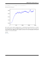
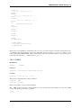
2.3.1 Gnuplot
Gnuplot (http://www.gnuplot.info/) is a portable command-line driven graphing utility, and it is a useful tool for
showing the outputs of FARGO3D. Here you have an example on how to load the outputs of FARGO3D on our
two-dimensional first run.
The command line should be similar to:
$: gnuplot
Version 4.6 patchlevel 1
last modified 2012-09-26
.
.
.
gnuplot> set palette rgbformulae 34,35,36
gnuplot> set logscale cb
gnuplot> nx = 384; ny = 128
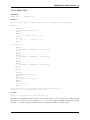
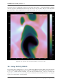
gnuplot> plot[0:nx-1][0:ny-1] "./gasdens10.dat" binary array=(nx,ny) format="%lf"
with image notitle
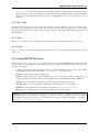
and you should see an image similar to:
Figure 2.1: Gnuplot image of the first run (gas surface density), output number 10.
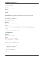
2.3.2 GDL/IDL
GDL (GNU Data Language - http://gnudatalanguage.sourceforge.net/) is an open-source package similar to IDL,
but it is free and has similar functions. The command line should be similar to:
$: gdl
GDL - GNU Data Language, Version 0.9.2
.
.
.
GDL> openr, 10, ’gasdens10.dat’
GDL> nx = 384
GDL> ny = 128
GDL> rho = dblarr(nx,ny)
GDL> readu, 10, rho
GDL> rho = rebin(rho, 2*nx, 2*ny)
2.3. First run
7
FARGO3D User Guide, Release 1.1
GDL> size = size(rho)
GDL> window, xsize=size[1], ysize=size[2]
GDL> tvscl, alog10(rho)
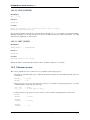
and you should see an image similar to:
Figure 2.2: GDL image of the first run (gas surface density), output number 10.
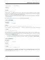
2.3.3 Python
Python (http://www.python.org/) is one of the most promising tool for data analysis in the scientific community.
The main advantages of Python are the simplicity of the language, and the power of its many libraries. Data
reduction of FARGO3D data is straightforward with the numpy package (http://www.numpy.org/). Also, making
plots is extremely easy with the help of the matplotlib package (http://matplotlib.org/). We strongly recommend
to use the interactive python-shell called IPython (http://ipython.org/).
Here, you have an example on how to work in an interactive IPython shell:
$: ipython --pylab
IPython 1.0.0 -- An enhanced Interactive Python.
.
.
.
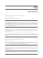
In [1]: rho = fromfile("gasdens10.dat").reshape(128,384)
In [2]: imshow(log10(rho),origin=’lower’,cmap=cm.Oranges_r,aspect=’auto’)
In [3]: colorbar()
You should see an image similar to (inside a widget):
Figure 2.3: Matplotlib image of the first run, output number 10.
8
Chapter 2. First Steps
FARGO3D User Guide, Release 1.1
2.3.4 More tools
The is a lot of software for reading and plotting data, but in general you need to have an ASCII file of the data.
In the utils directory, you will find some examples on how to transform the data into a human readable format,
written in different languages. If you are working with a large data set, this option is not recommended. It is
always a good choice to work with binary files, your outputs are lighter and the reading process is much faster.
Warning: Using ASCII format is very slow and should never be used for high resolution simulations or a 3D
run.
Note that FARGO3D can also produce data in the VTK format, which can be inspected with software such as
VISIT. This feature of FARGO3D will be entertained later in this manual.
2.4 First parallel run
Until now, we did not need external libraries to compile the code, but if we want to build a parallel version of the
code, we must have a flavor of MPI libraries on our system.
Note: FARGO3D was successfully tested with:
• OpenMPI 1.6/1.7
• MPICH2/3
• MVAPICH2 2.0
with similar overall performance for the CPU version of the code.
As we do not use any version-dependent features of MPI, we expect the code to work with any version of MPI.
There are however some special features of MVAPICH 2.0 and OpenMPI 1.7 related to CUDA interoperability
that are discussed later in this manual, and that are useful exclusively for GPU builds.
If you are running on a standard Linux installation, with a standard working MPI distribution, you have to issue:
$: make PARALLEL=1
or the corresponding shortcut:
$: make para
At the end of the process, you will see a message, telling you that the compilation was performed in parallel. Now,
you can run the code in parallel:
$: mpirun -np 4 ./fargo3d -m setups/fargo/fargo.par
If your computer have at least four physical cores, you should see a speed-up of a factor ~4.
Note: Open-MPI-Installation on Ubuntu systems. If you have Ubuntu, these lines install a functional version of
OpenMPI:
$: sudo apt-get install openmpi-bin
$: sudo apt-get install openmpi-common
$: sudo apt-get install libopenmpi-dev
You must accept all the installation requirements. A similar process could be done for MPICH. This process is
very similar on other Linux-systems with a package manager.
Warning: The -m flag that we have used so far in the command line instructs FARGO3D to merge all data
from all processes when writing them to the disk. which makes much easier its subsequent reduction. In
general, it is a good idea to always use this flag.
2.4. First parallel run
9
FARGO3D User Guide, Release 1.1
2.5 First GPU run
Warning: We assume you have installed CUDA and the proper driver on your system. You can test if the
driver works correctly by running nvidia-smi in a terminal. It is also a good idea to run a few examples of
the NVIDIA suite to ensure that your installation is fully functional.
Running FARGO3D in GPU mode is similar to the first parallel run. The only important thing is to know where
CUDA is installed. FARGO3D knows about CUDA by the environment variable CUDA defined in your system. If
you do not have the CUDA variable defined, FARGO3D assumes that the default path where CUDA is installed is
/usr/local/cuda. If this is not the right place, modify your .bashrc file and add the following line:
‘‘export CUDA=Your CUDA directory‘‘
Warning: The above example assumes that you use the bash shell.
After that, we are ready to compile the code:
$: make PARALLEL=0 GPU=1
or the corresponding shortcut:
$: make PARALLEL=0 gpu
Warning: you cannot combine shortcuts in the command line. You could for instance issue make seq
GPU=1 instead of the instruction above (seq stands for PARALLEL=0), but make seq gpu would fail.
Note: Additional information
We assume here that you followed the whole sequence of examples of this page, so that your previous run was
a parallel CPU run. Build options (such as PARALLEL=1) are sticky, so that they are remembered from build
to build until their value is explicitly changed. Since we want here a sequential built for one GPU, we need to
explicitly reset the value of PARALLEL to zero.
Another option is to issue:
make mrproper
which resets all sticky built options to their default values, and after that issue:
make gpu
You will see at the end of the building process the message:
FARGO3D SUMMARY:
===============
This built is SEQUENTIAL. Use "make para" to change that
This built can be launched on
a CPU with a GPU card (1 GPU only).
SETUP:
’fargo’
(Use "make SETUP=[valid_setup_string]" to change set up)
(Use "make list" to see the list of setups implemented)
(Use "make info" to see the current sticky build options)
telling you that the build is sequential and should be run on a GPU. To run it, simply type:
10
Chapter 2. First Steps
FARGO3D User Guide, Release 1.1
$: ./fargo3d -m setups/fargo/fargo.par
Before the initialization of the arrays, you will see a block similar to:
=========================
PROCESS NUMBER
0
RUNNING ON DEVICE Nº 0
GEFORCE GT 520
COMPUTE CAPABILITY: 2.1
VIDEO RAM MEMORY: 1 GB
=========================
It is the information about the graphic card used by FARGO3D. If you see some strange indications in these
lines (weird symbols, an unreasonable amount of memory, etc), it is likely that something went wrong. The most
common error is a bad device auto-selection.
Warning: In the jargon of GPU computing, the device is the name for a given GPU. We shall use indistinctly
these two terms throughout this manual.
If you need to know the index of your device, you can use the nvidia-smi monitoring software:
$: nvidia-smi
You may then explicitly specify this device on the command line (here e.g. 0):
$./fargo3d -m -D 0 setups/fargo/fargo.par
In general, expensive cards support detailed monitoring, but at least, the memory consumption will be given even
for the cheapest ones. Also, you can check the temperature of your device. An increasing temperature is a good
indication that FARGO3D is running on the desired device.
Note: Useful comments
Note 1:
If you cannot run on a GPU after reading the above instructions, you should try to check the index of your device
(normally it is 0 is you have only one graphic card) with nvidia-smi:
$: nvidia-smi
+------------------------------------------------------+
| NVIDIA-SMI 4.310.44
Driver Version: 310.44
|
|-------------------------------+----------------------+----------------------+
| GPU Name
| Bus-Id
Disp. | Volatile Uncorr. ECC |
| Fan Temp Perf Pwr:Usage/Cap| Memory-Usage
| GPU-Util Compute M. |
|===============================+======================+======================|
|
0 GeForce GT 520
| 0000:01:00.0
N/A |
N/A |
| 40%
37C N/A
N/A / N/A | 18% 182MB / 1023MB |
N/A
Default |
+-------------------------------+----------------------+----------------------+
+-----------------------------------------------------------------------------+
| Compute processes:
GPU Memory |
| GPU
PID Process name
Usage
|
|=============================================================================|
|
0
Not Supported
|
+-----------------------------------------------------------------------------+
And the number of the GPU in this case is 0. So, you could try to run FARGO3D forcing the executio
$: ./fargo3d -mD 0 setups/fargo/fargo.par
Note 2:
2.5. First GPU run
11
FARGO3D User Guide, Release 1.1
We have used two sticky flags: PARALLEL and GPU, and after some time you may wish to know which ones are
activated. In order to know the current status of the executable, issue:
$: make info
Current sticky build options:
PROFILING=0
RESCALE=0
SETUP=fargo
PARALLEL=0
FARGO_DISPLAY=NONE
FULLDEBUG=0
UNITS=0
GPU=1
DEBUG=0
MPICUDA=0
BIGMEM=0
You will see the meaning of each flag later on in this manual.
All the information about how to open and visualize your fields is still valid. While the computation was done on
the GPU, all necessary data transfers were run in a transparent manner from the GPU to the CPU before a write to
the disk. For you, nothing changes, except the execution speed.
2.6 First Parallel GPU run
The same ideas as before can be used for running FARGO3D on multiple GPUs. But we cannot give a set of
instructions because they are cluster-dependent. In the next sections you will learn how to run FARGO3D on a
large cluster and have each process select adequately its device, according to your configuration. When you know
how to work with the internal SelectDevice() function, you will be able to work with FARGO3D on a cluster
of GPUs.
You could try to run with MPI over one GPU. Of course it is a bad idea for performance reasons, but it shows if all
the parallel machinery inside FARGO3D works. (Actually, for developing an MPI-CUDA code, you do not need
more than one thread and one GPU card!).
Try the following:
$: make mrproper
$: make PARALLEL=1 gpu
$: mpirun -np 2 ./fargo3d -m setups/fargo/fargo.par
If all goes fine, that is to say if the output looks correct, FARGO3D is working with MPI and GPUs. The next step
is to configure it to run on a cluster of GPUs, using as many different GPUs as possible. We will learn how to do
that later on in this manual
12
Chapter 2. First Steps
CHAPTER
THREE
DIRECTORY TREE
FARGO3D was developed as a general code. It solves a set of coupled differential equations on a mesh. Because
it was developed as a general solver, it is necessary to keep certain general features isolated from other, more
specific ones (that correspond to a specific problem).
A simple example of that is the initial condition (IC) of a problem. Obviously, the IC is a problem-dependent
feature, and a mechanism is needed to keep it isolated from another problem. Touching the main structure of the
code only to change the IC is not a good idea (yes, you can, but this is ugly, error prone and wreaks havoc with
versioning systems). This kind of problem is solved using the concept of SETUPS, and with the help of the VPATH
Makefile variable. If you know the RAMSES code (http://www.ics.uzh.ch/~teyssier/ramses/RAMSES.html), you
will see that we use the same patch concept.
Warning: In practice, when using FARGO3D you do not need to know about the VPATH variable, but if you
want to develop some new features, it is a good idea to keep in mind that it is used under the hood.
Another problem is related to the different modules of the code. For example, in some situations we need to use
the MHD module, but for another set of problems, the MHD is irrelevant. In order to avoid a lot of logical run time
tests inside the code (if‘s), we prefer to use MACROCOMMAND variables. These variables are interpreted prior
to compilation time, by the so-called preprocessor, and activate/deactivate certain features (lines) of the code,
allowing a tailor-made executable, built for a specific problem. All these variables are activated from the Makefile
(they are defined actually in the .opt files that we shall see below).
The most important file to ultimately build a FARGO3D executable is obviously the Makefile. For this reason,
there is a section devoted to this particular file. But, because FARGO3D uses a lot of scripting at compilation
time, the process of building the code does not simply reduce to the Makefile. We refer to the FARGO3D building
process as “the make process”.
A given instance of FARGO3D has many different properties, and storing each one in an organized manner is
achieved through a number of different subdirectories. In this section we give a brief explanation about each one.
3.1 Directories
3.1.1 src/
The directory where the main sources are stored is the src/ directory. Inside it, you will find all the files related
to the initialization, evolution and visualization of the data. All the sources are pure C files, plus some headers and
a very few CUDA files. Also, in this folder you can find the main makefile (src/makefile). This makefile should
never be called directly. All the fundamental changes to the code must to be done here.
3.1.2 scripts/
In the scripts/ directory you will find the fundamental python-scripts used at compilation time. There are
scripts for:
• Defining variables.
13
FARGO3D User Guide, Release 1.1
• Analyzing boundary conditions.
• Analyzing and defining units.
• Generating CUDA files automatically.
• Improving CUDA blocks.
• Accelerating the make process (executing the makefile in parallel).
• Making general tests (mandatory for new improvements).
3.1.3 bin/
This directory is empty by default, but during compilation, this is where all the object files and script-residual data
are stored. In practice, this directory is useful for avoiding a mixing between sources and objects, a very useful
behavior when your are developing new routines.
3.1.4 outputs/
The outputs/ directory is the default output directory for all the FARGO3D standard setups. As you
could see in the first run, the data were stored in outputs/fargo. By default all the data is stored in
outputs/setup_name, where setup_name is one of the setups in the setups/ directory.
3.1.5 setups/
This directory is where all the different setups are. By default, the make process looks here if the setup is defined,
eg:
$: make SETUP=otvortex
After that, the makefile will search inside setups/ whether there is a directory called setups/otvortex.
Inside the otvortex/ directory we find all the files necessary to set up the problem and build the code.
3.1.6 planets/
Inside this directory are the default planetary system files to run a simulation with one or several planets, considered as point-like masses that interact between them and with the disk (onto which they act as an external
potential). The syntax of planetary files is for the former FARGO code. It is not mandatory to store your planetary
data here, but it is recommended.
3.1.7 std/
the name std comes from “standard”. This directory stores all the standard configuration files. In this version,
these are:
• boundaries.txt: where the boundary conditions are defined.
• boundary_template.c: A build helper for the boundaries scripting.
• centering.txt: A file describing the centering of the different fields with respect to the mesh (helper
for boundary conditions scripting).
• defaultflags: A file with all the default flags for the make process.
• std.par: Default parameters. It is used when you have not defined the value of a certain parameter in
your parameter file. It is used for compatibility with some specific problems related to disks simulations
and some plot-related parameters.
• standard.units: The scaling rules for all standard real variables of the code.
14
Chapter 3. Directory tree
FARGO3D User Guide, Release 1.1
• func_arch.cfg: The standard architecture file. This file selects where each function will run (CPU or
GPU). It only has sense if the compilation was done with GPU-Compatibility (GPU=1). By default, all the
function run on the GPU, but this file is a great tool for debugging the code (one of the best tools to develop
a kernel!).
3.1.8 test_suite/
This directory was developed to ensure a stable development of the code. Here there is a set of test files written
in python. All of them use the script test.py. They are easy to understand. The main idea is: if your recent
developments pass all the tests, at least, your new improvements do not interfere with the main code and do not
alter its behavior.
3.1.9 utils/
Here is a set of routines to analyze the data. The content inside is self-documented. Feel free to explore it.
3.1.10 doc/
The doc/ directory is where these documentation files reside. Also, here are some files related with the licence
of the code.
3.2 setups/SETUP directory
The directory setups/SETUP is one of the most complex directories in FARGO3D. The complexity arises
because inside are stored all the information required for a given, specific problem. The extensive list of the files
stored for each setup is:
• condinit.c: this is the file where the initial conditions are written. Thanks to the use of the VPATH variable
in the makefile, this file supersedes the file src/condinit.c of the main source.
• SETUP.par: the parameters required for this setup.
• SETUP.opt: all the directives for the makefile (this is were you decide the number of dimensions, the
equation of state, the geometry, whether you use orbital advection -aka FARGO algorithm-, MHD, etc.)
• SETUP.bound: set the boundary conditions used in the setup (taken from boundaries.txt).
• SETUP.mandatories: A list of parameters that must be always explicited in your .par files.
• SETUP.units: The scale rules for the parameters not explicited in std/standard_units.
• SETUP.objects: Additional objects you want to include. (Your own developments).
Warning: Any file here has priority over the file with same name in the src/ directory. So, in theory, inside
a SETUP directory, you could have a complete copy of the src/ directory, and the make process will be
done with this sources, but in practice, only a few files are needed, for example, depending on your needs:
resistivity.c, potential.c, etc.
3.2. setups/SETUP directory
15
FARGO3D User Guide, Release 1.1
16
Chapter 3. Directory tree
CHAPTER
FOUR
MAKE PROCESS
Building the code is achieved simply by invoking the Makefile in the main directory. The Makefile contains the
set of instructions that builds the executable, normally called “fargo3d” according to a specific setup and with
proper instructions for generating a CPU, GPU, sequential or parallel built. This Makefile is not standalone. A set
of scripts was developed in order to simplify the building process. These scripts do all the hard work. Most users
will not need to know the different stages of a build, but we give here the detail of what happens when you issue
make [options] in the main directory.
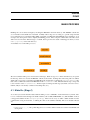
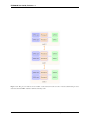
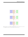
A schematic view of the make process is:
We can see that the make process involves three main steps. When we type make in the main directory, we spawn
the first step, that is we execute the Makefile. All the shortcut rules, cleaning rules and testing rules are defined
within. The second step is spawned by the Makefile itself, and amounts to running the scripts/make.py file,
that works as a link between the main Makefile and the src/makefile file. The third and last step corresponds
to the execution of the src/makefile . All the scripts are managed at this stage (automatic conversion of C to
CUDA, analysis of boundary conditions and scaling rules, etc.)
4.1 Makefile (Stage1)
As we have just seen the first file related with the make process is “Makefile” in the main directory. Inside, there
is a set of instructions that manages the build variables (such as GPU, PARALLEL, etc.) This makefile works as
a wrapper that further invokes scripts/param.py. There are two ways to define a build variable from the
command line: using shortcut rules, or defining the value of the variables manually. The set of variables allowed
are:
• PROFILING: [0,1] The profiler flags and a set of timers will be activated. Useful for benchmarks and
development.
17
FARGO3D User Guide, Release 1.1
• RESCALE: [0,1] Activates a rescaling of the (real) parameters of the parameter file to certain units. The
numerical values used for this rescaling depends on the value of the build variable UNITS. The output are
all done with the new units.
• SETUP: Selects the proper directory where your setup is. A list will be shown if you type make list.
• MPICUDA: [0,1] Activates the peer2peer/uva MPI-Communications between different devices. Only
compatible with MVAPICH2 2.0 and OpenMPI 1.7. (Strongly recommended)
• FARGO_DISPLAY: [NONE,MATPLOTLIB] Run time visualization of your fields using python-numpymatplotlib packages.
• DEBUG: [0,1] The code will be compiled in debug mode. The main change is the flag “-g” at compilation time. No optimization is performed in this mode.
• FULLDEBUG: [0,1] The code runs in full debug mode. Similar to debug mode, but the merge flag (-m)
is not allowed. All the fields are dumped with their ghosts cells (buffers).
• UNITS: [0,MKS,CGS] How the units are interpreted by the code. See the unit section for further details.
• GPU: [0,1] Activates a GPU compilation.
• PARALLEL: [0,1] Activates the use of the MPI Libraries.
• BIGMEM: [0,1] Activates the use of the global GPU memory to store light (1D) arrays (which are
otherwise stored in the so-called constant memory on board the GPU). Normally, it is needed when your
simulation exceeds ~750 cells in some direction. This feature is device-dependent. Typically, a 3D run with
mesh size 500*500*500 does not require BIGMEM=1, but a 2D run with mesh size 50*1000 does. However,
when BIGMEM=1 is not required, you may activate it. Perform some benchmarking to check which choice
yields faster results. This is very problem and platform dependent.
• jobs/JOBS: [N] where N is the number of processes that you want to spawn for building the code. By default
N=8. This option is much needed when working with CUDA. The building process of CUDA object files is
by far the most expensive stage of building a GPU instance of FARGO3D, as you will soon realize.
All these variables must to be defined by: make VARIABLE=VALUE.
The shortcut rules are invoked with the command make option, where option can be:
• cuda/nocuda, gpu/nogpu –> GPU=1/0
• bigmem/nobigmem –> BIGMEM=1/0
18
Chapter 4. Make Process
FARGO3D User Guide, Release 1.1
• seq/para –> PARALLEL=0/1
• debug/nodebug –> DEBUG=1/0
• fulldebug/nofulldebug –> FULLDEBUG=1/0
• prof/noprof –> PROFILING=1/0
• mpicuda/nompicuda –> MPICUDA=1/0
• view/noview –> FARGO_DISPLAY=MATPLOTLIB/NONE
• cgs/mks/scalefree –> UNITS=CGS/MKS/0
• rescale/norescale –> RESCALE=1/0
• testlist –> A list of the tests implemented.
• testname –> the test called name.py, found in test_suite, will be executed.
• blocks –> special syntax: make blocks setup=SETUPNAME. Performs a detailed study of the performance of your graphic card with respect to the size of the CUDA blocks. This test will be done for each
GPU function. The result is stored in setups/SETUPNAME/SETUPNAME.blocks (go to the section “Increasing the GPU performance”). A build is performed with a default block size if this file does not exist,
so you do not have to worry about this feature at this stage. However, remember that it may increase the
performance up to ~20 %.
• clean –> Cleans the bin/ directory. Recommended when you switch to another SETUP.
• mrproper –> Removes all the data related to some specific make configuration. All the code is restored to
its default. The outputs directory will not be touched.
4.2 scripts/make.py (Stage2)
The second step in the building process is to call make.py. This file does not need a manual invocation, and is
launched from the main Makefile (stage1). In general, the compilation process is expensive when you are working
with CUDA files. For this reason, a parallel make process is highly desirable. Normally, a general Makefile
can handle parallel compilation, but in the FARGO3D case (that uses a lot of scripting) some race conditions
could be appear in parallel Makefiles. Since the GNU make utility does not have a proper way to avoid such
problem, we developed an interface between Makefile and src/makefile to do all the building process in the right
order: first invoking the scripts to build all the headers and variable declarations and then a parallel execution of
src/makefile. Also, make.py keeps track of the last flags used in the last built (sticky options). All this
information is stored in the hidden file std/.lastflags.
4.2. scripts/make.py (Stage2)
19
FARGO3D User Guide, Release 1.1
4.3 src/makefile (Stage3)
The third and last step in the building process is to call src/makefile, which is done by scripts/make.py.
The role of this makefile is to build the executable, normally called fargo3d in the main directory. All the calls
to scripts are done here. Inside there are a set of rules for making the executable in the correct sequence. You may
have a look through these different rules, which are self-documented by their names.
There is a set of system-configuration blocks, that allows to build FARGO3D on different platforms with the same
makefile. This configuration blocks are selected by using the environment variable called FARGO_ARCH (the
same as for the FARGO code). Also, inside this makefile are defined a lot of useful variables. Here is where the
structure of the code is defined, and where the variable VPATH is specified. This variable is extremely powerful,
and if you want to extend the FARGO3D directory structure, you should learn about the use of this variable (GNU
Make Reference Guide).
Another important set of variables are:
• MAINOBJ: The name of all the CPU objects that will be linked with the final executable. All new source
file in the code must to be included in this variable (with the .o extension, instead of .c)
• GPU_OBJ: The name of the static kernels used in the code. In practice, you will never need have to touch
it. By static we mean that these few kernels are not generated automatically from the C code by a Python
script.
• GPU_OBJBLOCKS: The name of the objects that will be generated by the script c2cuda.py. Note all of
them must have the suffix _gpu.o, with a prefix that is the one of the corresponding C file. This is very
important, because the rule that generates CUDA-files from C-files uses the suffix of the object name. In the
tutorial on how to develop a GPU-Routine (function) this will be presented in more detail. All the functions
that must be generated automatically from C code at build time must appear as a list in this variable.
4.4 FARGO_ARCH environment variable
FARGO3D is a multi-platform code, and can run on a modern cluster of GPUs but also on your personal computer,
even without a GPU. For the ease of use, we adopt a computer-dependent makefile scheme, managed by the
environment variable FARGO_ARCH.
You can see in src/makefile a group of lines similar to:
#LINUX PLATFORM (GENERIC)
#FARGO_ARCH must be set to LINUX
CC_LINUX
= gcc
SEQOPT_LINUX = -O3 -ffast-math
PARAOPT_LINUX = ${SEQOPT_LINUX}
PARACC_LINUX = mpicc
LIBS_LINUX
= -lm
INC_LINUX
=
NVCC_LINUX
= nvcc
PARAINC_LINUX =
PARALIB_LINUX =
These lines are telling the makefile where the libraries are and which compilers will be used. In the LINUX case
(default case), we are not including any parallel library to PARALIB and any header to PARAINC because we are
assuming they are in your LD_LIBRARY_PATH, or they are installed in the default places. In general, in your
cluster you should have something similar to:
#FARGO_ARCH must be
CC_MYCLUSTER
=
SEQOPT_MYCLUSTER =
PARAOPT_MYCLUSTER =
PARACC_MYCLUSTER =
LIBS_MYCLUSTER
=
INC_MYCLUSTER
=
20
set to MYCLUSTER
/bin/gcc
-O3 -ffast-math
${SEQOPT_LINUX}
/bin/mpicc
-lm
Chapter 4. Make Process
FARGO3D User Guide, Release 1.1
NVCC_MYCLUSTER
= ${CUDA}/bin/nvcc
PARAINC_MYCLUSTER = -I/${MPIDIR}/include
PARALIB_MYCLUSTER = -L/${MPIDIR}/lib64
Where MPIDIR and CUDA are variables pointing to the place where MPI and Cuda are installed.
To use the FARGO_ARCH variable, you have two options:
• define FARGO_ARCH before compiling the code.
• define FARGO_ARCH in your personal .bashrc or .tcshrc file (depending on your shell).
If you do not have a standard Linux distribution, do not forget to export the variable FARGO_ARCH in your
~/.bashrc file:
$: vi USER_DIR/.bashrc
and add the following line:
export FARGO_ARCH=MYCLUSTER
where MYCLUSTER is only an example name. You should modify it to match the name that you defined in the
src/makefile. This file is provided as is with a few examples that you may adapt to your own needs.
4.4. FARGO_ARCH environment variable
21
FARGO3D User Guide, Release 1.1
22
Chapter 4. Make Process
CHAPTER
FIVE
BOUNDARIES
Boundary conditions in FARGO3D can be selected only for the Y and Z directions, since in X the mesh is always
considered periodic. It is because FARGO3D was mainly designed for azimuthal-periodic planetary disks, with a
cost-effective orbital advection (aka FARGO) algorithm. Albeit that this limitation may seem strong in practice,
there are lots of situations where you can assume your 3D problem to be periodic along a given direction. If you
can not do that, unfortunately there is no way to avoid this limitation with the present version of the code.
The boundary conditions (BCs) are handled by the script boundparser.py. We have developed a metalanguage to handle them. Although this may seem quite a futile investment, it soon appeared to be much needed as
we were developing the code. We had initially left the treatment of BCs on the CPU, even for GPU builds. We
thought that the filling of the ghost zones by the CPU would have negligible impact on the overall speed of the
code. This, however, turned out to be untrue: the CPU-GPU communication overhead, and the slowness of CPU
calculations lowered the code performance significantly. We therefore decided to deal with BCs in the exact same
way as with other time consuming routines, which can be translated automatically to CUDA, so as to run on the
GPU. This implied some syntax constraints on the associated C code, which would have made the development
of a variety of boundary conditions on the four edges of the mesh a time consuming and error prone process (yes,
four, because they are specified only for Y and Z). For this reason, we have chosen to write a script that produces
the C code for a given set of boundary conditions, with all the syntactic comments needed to subsequently translate
it to CUDA.
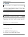
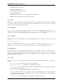
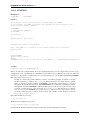
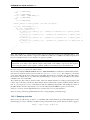
5.1 How are boundary conditions applied?
The boundary conditions are applied just after the initialization of a specific SETUP (before the first output),
and subsequently, twice per time step. Boundary conditions are applied to all primitive variables, and to the
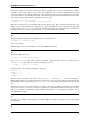
electromotive forces (EMFs). All boundary conditions are managed by the routine FillGhosts(), inside
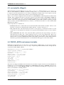
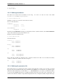
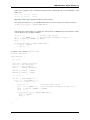
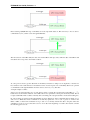
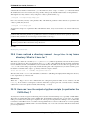
src/algogas.c. Below, we depict schematically how cells of the active mesh are mapped to the ghost zones.
The last (third) ghost cell is filled with the first active one, the second ghost cell is filled with the second active
one, and finally the first ghost cell is filled with the third active cell.
Note: Note that we do not consider the mesh periodicity along a given direction as a proper boundary condition,
in the sense that no ad hoc prescription has to be used to fill the corresponding ghost zones. Rather, a mesh
periodic along a given dimension has no boundary in this dimension, and this property is assigned to the mesh
in the parameter file (and not in the boundary files of the setup that we present in detail below) by the use of the
Boolean parameters PeriodicY and PeriodicZ, which default to NO. In the boundary files that we present
hereafter, you will therefore see BC labels such as SYMMETRIC, OUTFLOW, etc., but never PERIODIC.
Note: We note on the figure above that we have three rows of ghost cells. The number of rows depends on
the problem, and on how frequently communications are performed within a time step. There is a trade off
between the number of rows (large buffers slow down the calculations and the communications) and the number
of communications. The number of ghosts is defined in src/define.h around line 40 et sq.
23
FARGO3D User Guide, Release 1.1
Figure 5.1: Schematic view of how the boundaries are applied. We note that the buffer (or ghost) zones are three
cells wide.
24
Chapter 5. Boundaries
FARGO3D User Guide, Release 1.1
5.2 boundparser.py
In order to work with boundaries, we have developed a script called boundparser.py, that reads a general
boundary text file and converts it into a C file, properly commented to be subsequently converted into a CUDA
file. boundparser.py works with four files, called:
• setup.bound
• boundaries.txt
• centering.txt
• boundary_template.c
(note: these last three files can be in your setup directory, or by default, the script takes those of the std/
directory, as prescribed by the VPATH variable.)
boundparser.py reads the information inside the setup.bound file, and compares it with the information in
boundaries.txt and centering.txt. Finally, it builds a set of C files that apply the boundary conditions
(called [y/z][min/max]_boundary.c) with a proper format, given by boundary_template.c. We will not give a
detailed description on how boundparser.py works, but it is not difficult to understand the script if you are
interested in its details.
The key to developing boundary conditions is to understand the structure of setup.bound and
boundaries.txt file. Both files are in the same format, described below.
5.3 Boundaries files format
boundaries.txt, centering.txt and setup.bound files have the same format. All are case insensitive, and have two levels of information: a main level and an inner level. Also, comment lines are allowed. The
general structure of the format is:
# Some header
#-------LEVEL1_a:
Level2_a:
Level2_b:
Level2_c:
Level2_d:
Some_data1_a
Some_data1_b
Some_data1_c
Some_data1_d
#A comment
# A comment line
LEVEL1_b:
Level2_a:
Level2_b:
Level2_c:
Level2_d:
Some_data2_a
Some_data2_b
Some_data2_c
Some_data2_d
etc...
5.4 centering.txt
Special care must to be taken to the centering of data. Not all data are defined at the same location in FARGO3D.
In order to write automatically boundary conditions in a given direction (Y/Z), it is necessary to know which
fields are centered or staggered in this direction. This information is taken by boundparser.py from
centering.txt. This file uses the same format described above, and uses a particular set of instructions.
The allowed values are:
5.2. boundparser.py
25
FARGO3D User Guide, Release 1.1
• LEVEL1 –> The name of a Field Structure inside the code (eg: Density, Vx, Bz, etc...).
• Level2 –> the word “Staggering”
• data –> C,x,y,z or a combination of xyz (eg: xy, yz, xyz)
C is short of “centered”, meaning that the field is a cube-centered quantity. The meaning of x is staggered in x,
that is to say the corresponding quantity is defined at an interface in x between two zones, rather than in the middle
of two subsequent interfaces. By default, the field value is assumed centered along each direction that does not
appear explicitly in the centering definition.
Let us have a look at some lines of centering.txt:
Density: Staggering: C
Bz: Staggering: z
Emfz: Staggering: xy
The first two lines specify that the density is a cube centered quantity. The following two lines specify that the
magnetic field in the z-direction is centered in x and y, but staggered in z (ie defined at the center of an interface
in z). Finally, the last two lines indicate that the EMF in z is centered in z, but staggered in x and y. It is therefore
a quantity defined at half height of the lower vertical edge in x and y of a cell.
All primitive variables and the EMF fields are defined by default in std/centering.txt. If you create a new
primitive field in the code, you should specify its correct centering in std/centering.txt if you want to
create boundary conditions for this field.
5.5 boundary_template.c
This file is taken as a template for building automatic boundary condition C files . You should never have to
deal with it. Also, it contains all the information for subsequent building of the CUDA files. If you need special
boundary conditions, you could try modifying this file first. As long as you do not alter the lines beginning with
“%”, you can modify this template. This kind of modification should be made by an advanced user.
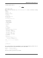
5.6 boundaries.txt
This file is the core file for the boundary condition. The main idea is to provide a way to the user to define a
boundary prescription in as user-friendly a manner as possible. Let us begin with a simple example. Assume that
we want to define a boundary condition that we call SYMMETRIC, which simply consists in copying the data of
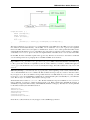
an active cell into the ghost zone. We represent schematically what is intended on this diagram:
|
|
|
|
^
|
ghost
zone
|
|
^
|
active
zone
The active zone contains a value, that we call, arbitrarily, active
|
|
|
|
^
|
ghost
zone
active
|
|
^
|
active
zone
We want to set the value of the ghost zone to the same value, that is we want:
26
Chapter 5. Boundaries
FARGO3D User Guide, Release 1.1
|
|
active
|
|
active
^
|
ghost
zone
|
|
^
|
active
zone
Therefore we represent this boundary condition with the following, rather intuitive line of code:
|
active
|
active
|
Assuming for the moment that this boundary condition applies to centered variables, we would finally write the
following piece of code in boundaries.txt to define our SYMMETRIC boundary condition:
SYMMETRIC:
Centered:
|
active
|
active
|
The right “cell” always represent the active cell, and the left “cell” the corresponding ghost cell. The string active
could be actually any string:
SYMMETRIC:
Centered:
|
value
|
value
|
If we wish to have an anti-symmetric boundary condition (that is to say that we set the ghost value to the negative
of its active counterpart):
|
-active
|
active
|
Should we want to set the ghost value to twice the active zone’s value:
|
2.0*foo
|
foo
|
Or if we wish to set it to some predefined value (say that you have a supersonic flow of uniform, predefined density
0.12 g/cm^3 entering the mesh, and you work in cgs):
|
0.12
|
whatever
|
in which case the value whatever is never used. Naturally, it is much better to use a parameter (say, RHO0, that
you define in your parameter file):
|
’RHO0’
|
whatever
|
We shall come back to the use of the quotes later on in this section.
This, in a nutshell, is how we define boundary conditions in the code.
Now, assume that we want to have an anti-symmetric boundary condition on the velocity perpendicular to the
boundary. The situation is a bit different than the one described above, because this field is staggered along the
dimension perpendicular to the mesh. That is, we have:
|
|
|||
|
|||
|
^
value
|
edge of
active mesh
As shown on this diagram, the value is defined at the interface, and not at the center as previously. The triple
vertical line delineates the edge of the active mesh. What we intend is the following:
|
|
-value
|||
|||
^
|
5.6. boundaries.txt
|
|
value
27
FARGO3D User Guide, Release 1.1
edge of
active mesh
but this leaves yet unspecified the value at the edge of the active mesh, which should be set here to zero (it has to
be its own negative):
|
|
-value
|||
|||
0
|
|
value
Eventually we have to specify one extra value with respect to the centered case. Our boundary condition is
therefore coded as:
ANTISYMMETRIC:
Staggered:
|
-value
|
0
|
value
|
If the | (pipe) symbol could be thought of as representing the zones interface for the centered case, it is no longer
the case in the staggered case. In any case, we will always have two “cells” in the BC code for a centered quantity,
and three “cells” in the BC code for a staggered quantity, regardless of the number of rows in the ghosts. The
matching between an active cell and its corresponding ghost zone is as shown on the figure at the beginning of this
section.
We sum up this information: the file boundaries.txt contains a two level description that obeys the general
following rule:
• LEVEL1 –> the name of the boundary. It is an arbitrary name, defined by you.
• Level2 –> the word “Centered” or “Staggered”, followed by some data.
• data –> |some_text_1|some_text_2| or |some_text_1|some_text2|some_text3|
The rules in the ghost zone are as follows:
1. Any string used in the active zone that matches some part of the ghost zone string, will be replaced by the
active cell value.
2. Any string inside ‘’ will be textually parsed and converted to upper case. They are useful to match the
parameters of the parameter files, which are upper case C variables.
3. Any string that does not match rule 1 nor rule 2, will be textually parsed and converted to lower case.
Additionally, there is a set of indices helpers, for working with boundaries:
*jgh/kgh: The index of the y/z ghost cells.
*jact/kact: The index of the y/z active cells.
This helpers prove very useful to perform complex extrapolations at the boundaries. You can see examples in the
file std/boundaries.txt.
5.6.1 Examples:
Zero-gradient boundary:
Suppose we want to define a zero gradient boundary. That means we want to copy all the active zone in the ghost
zone for both centered and staggered meshes.
The syntax is as follows. It groups together the definitions that we have worked out above, for centered and
staggered fields:
SYMMETRIC:
Centered:
Staggered:
|active|active|
|active|active|active|
where the right active value will be copied without any modification to the ghost zone. Note that this boundary
definition is direction and side independent, ie it can apply to ymin, ymax, zmin and zmax.
28
Chapter 5. Boundaries
FARGO3D User Guide, Release 1.1
Keplerian extrapolation example
We define here a more complex boundary condition:
KEPLERIAN2DDENS:
Centered:
|surfdens*pow(Ymed(jact)/Ymed(jgh),’SIGMASLOPE’)|surfdens|
This line is equivalent to:
KEPLERIAN2DDENS:
Centered:
|active*pow(ymed(jact)/ymed(jgh),’sigmaslope’)|active|
as per the rules listed above.
What kind of action does this instruction correspond to ? It sets the value of the ghost zone to:
(︁
)︁𝛼
act
ghost value = Σactive 𝑅𝑅ghost
since Ymed stands for the radius of the center of zone, in a cylindrical setup.
The reader familiar with protoplanetary disk’s jargon and notation will easily recognize the radial extrapolation of
the surface density of the disk in the ghost zone, with a power law of exponent −𝛼 (𝛼 is dubbed SIGMASLOPE in
the parameters of FARGO3D), hence the string chosen to represent the value of the active cell (surfdens), although
at this stage nothing specifies yet to which variable this boundary condition should be applied. This is the
role of the file SETUP .bound.
5.7 SETUP.bound
This file must be located in the sub-directory of a given setup, and must have same prefix as the setup to which it
refers. For instance, in setup/fargo/, the file that specifies the boundaries is called fargo.bound.
The files that we described in the previous paragraphs are used to specify what transformation rule is used for an
arbitrary field (in boundaries.txt) depending on its centering, while the centering of all fields is specified by
std/centering.txt.
The SETUP .bound file now specifies the transformation rule to use for each physical variable. It obeys the
following general syntax:
• LEVEL1 –> The name of the field.
• Level2 –> The side of the boundary (ymin,ymax,zmin,zmax), and some data.
• data –> Boundary label (the label defined in boundaries.txt)
We show hereafter a few examples:
2D XY reflecting problem
We want to have a 2D isothermal fluid with periodic “boundary conditions” in X (as required in FARGO3D) and
reflecting boundary conditions in Y.
We have three primitive variables to which we must apply BCs. Those will only apply in Y (not in X because of
the periodicity, nor in Z because we have a 2D X-Y setup).
The setup.bound file should therefore look similar to:
Density:
Ymin:
Ymax:
SYMMETRIC
SYMMETRIC
Ymin:
Ymax:
SYMMETRIC
SYMMETRIC
Vx:
Vy:
5.7. SETUP.bound
29
FARGO3D User Guide, Release 1.1
Ymin:
Ymax:
ANTISYMMETRIC
ANTISYMMETRIC
where Vy is ANTISYMMETRIC in Y because we have reflection in the y-direction.
At build time, the script boundparser.py goes through this file. The first three lines instruct it to generate
C code to implement a boundary condition for the density field in ymin and ymax. It goes to the definition of
SYMMETRIC found in std/boundaries.txt. Two definitions are available: one for centered fields, the
other one for staggered fields. In std/centering.txt it finds that the density is centered (in y) and therefore
generates the C code corresponding to the centered case. The same thing occurs for Vx: it finds that this field
is centered in Y. Finally, the last three lines instruct it to generate C code for an ANTISYMMETRIC boundary
condition of Vy in Y. It finds in std/centering.txt that this field is staggered in Y, and generates the C code
corresponding to the definition:
| -value | 0 | value |
The C functions thus produced contain all the comments required to further conversion to CUDA, should the user
request a GPU built.
2D YZ reflecting problem
Now, a more complex example, with all directions (yet in 2D):
Density:
Ymin:
Ymax:
Zmin:
Zmax:
SYMMETRIC
SYMMETRIC
SYMMETRIC
SYMMETRIC
Vx:
Ymin:
Ymax:
Zmin:
Zmax:
SYMMETRIC
SYMMETRIC
SYMMETRIC
SYMMETRIC
Ymin:
Ymax:
Zmin:
Zmax:
ANTISYMMETRIC
ANTISYMMETRIC
SYMMETRIC
SYMMETRIC
Ymin:
Ymax:
Zmin:
Zmax:
SYMMETRIC
SYMMETRIC
ANTISYMMETRIC
ANTISYMMETRIC
Vy:
Vz:
Note: Note how the staggering is implicit in Vy/Vz boundaries.
An extensive list of examples can be found in the setups/ directory.
5.8 Common errors
This section will be developed later from users’ feed back.
The boundparser.py script is at the present time a bit taciturn, and may silently ignore errors which might be
a bit difficult to spot afterwards. Among them:
• Incorrect names or misprints.
• An incorrect centering.
30
Chapter 5. Boundaries
CHAPTER
SIX
MESH AND FIELDS
6.1 Mesh
The mesh consists of NX cells in X (hence azimuth in cylindrical and spherical geometries), NY+2*NGHY cells in
Y (radius in cylindrical and spherical geometries) and NZ+2*NGHZ cells in Z (colatitude in spherical geometry).
Here NGHY and NGHZ stand for the number of ghost or buffer zones next to the active mesh. If a direction is not
included in the setup (for instance Z in the 2D polar fargo setup), the corresponding value of NGHY/Z is set to
0.
The variables NX, NY and NZ are defined in the parameter file (they default to 1, so there is no need to define,
for instance, NZ in a 2D setup such as fargo, or NX in the 2D setup otvortex, which corresponds to the
Orszag-Tang vortex problem in Y and Z).
In practice, this mesh is split among processors, and locally (within the scope of a given process) the submesh
considered has size Nx, Ny+2*NGHY and Nz+2*NGHZ.
The information about cells coordinates is stored in 1D arrays
• [xyz]min(index)
• [xyz]med(index)
where min refers to the inner edge of a zone (in x, y or z) whereas med refers to the center of a zone (in x, y or z).
This notation should look familiar to former FARGO users.
Warning: [xyz][min/max](index) are not vectors, they are macrocommands. They must to be invoked with
(), not with [].
NGHY and NGHZ are preprocessor variables, defined in the file src/define.h.
Because we have a multi-geometry code, another set of secondary geometrical variables is defined (surfaces,
volumes). See the end of this section for details.
6.2 Fields
Fields are structures, and they can be seen as cubes of cells, of size equal to the mesh size. The location at which
a given variable is defined is [xyz]med if the field is [xyz]-centered, or [xyz]min if the field is [xyz]-staggered.
You can find a comprehensive list of the fields in src/global.h. The place where the fields are created is in
CreateFields(), inside src/LowTasks.c.
Internally, all fields are cubes written as 1D-arrays. So we need indices to work with the 3D-data. We have a set
of helpers defined in src/define.h. They are:
• l : The index of the current zone.
• lxp, lxm: lxplus/lxminnus, the right/left x-neighbor
• lyp, lym: lyplus/lyminnus, the right/left y-neighbor
31
FARGO3D User Guide, Release 1.1
• lzp, lzm: lzplus/lzminnus, the right/left z-neighbor
These helpers must be used with the proper loop indices:
int i,j,k;
for (k=z_lower_bound; k<z_upper_bound; k++) {
for (j=y_lower_bound; j<y_upper_bound; j++) {
for (i=x_lower_bound; i<x_upper_bound; i++) {
field[l] = 3.0;
field2[l] = (field1[lxp]-field1[l])/(xmed(ixp)-xmed(i));
}
}
}
//obviously some gradient c
where [kji] always means [zyx]-direction.
Warning: Do not change the order of the indices! The definition of l, lxp, lxm, etc. assumes the following
correspondence:
i->x, j->y, k->z
These helper are extremely useful. No explicit algebra has to be performed on the indices within a loop (but never
use or define a variable called l or lxp !...). Besides, the definition of l is also correct within GPU kernels
(for which the indices algebra is slightly different owing to memory alignment considerations), and this is totally
transparent to the user who should never have to worry about this.
In practice, a loop is similar to (isothermal equation of state):
int i,j,k;
for (k=0; k<Nz+2*NGHZ; k++) {
for (j=0; j<Ny+2*NGHY; j++) {
for (i=0; i<Nx; i++ ) {
pres[l] = dens[l]*cs[l]*cs[l];
}
}
}
Note: Note that the lines of code above do not evaluate, nor define l, which is used straight out of the box, since
it is a preprocessor macrocommand.
6.3 Working with fields
A field structure is defined as follows (in src/structs.h):
struct
char
real
real
};
field {
*name;
*field_cpu;
*field_gpu;
where we have stripped the definition of all extra lines not relevant at this stage. The name is a string that is used
to determine the name of output files. field_cpu is a pointer to a double or float 1D array which has been duly
allocated on the RAM prior to any invocation.
Similarly field_gpu is a pointer to a double or float 1D array which has been duly allocated on the Video RAM
prior to any invocation. The user should never have to invoke directly this field. Rather, C files will always make
use of the field_cpu, which will be automatically translated to field_gpu as needed during the C to CUDA
conversion.
Acceding a field value is generally done as follows:
32
Chapter 6. Mesh and Fields
FARGO3D User Guide, Release 1.1
struct Field *Density;
// Definition at the beginning of a function
real *density;
// real is either double or float.
density = Density->field_cpu;
...
later on in a loop:
...
density[l] = ....;
Note: Note that we define an “array of reals” straight away and subsequently only refer to it to manipulate cell
values. In order to avoid confusion, it is a good idea to have an upper case for the initial of Fields*, and lower case
for the corresponding real arrays.
6.4 Fields on the gpu
Similar techniques are used on the GPU, but we have made it totally transparent to the user, so unless you want to
program your CUDA kernels directly, you should never to worry about this.
6.5 Useful variables
For the handling of the mesh, a set of useful variables and macrocommands has been defined. An extensive list
with a description is given below:
Indices:
• l: The index of the current cell. It is a function of (i,‘‘j‘‘,‘‘k‘‘, pitch & stride).
• lxp: The index of the “right” neighbor in x of the current cell. It is a function of l.
• lxm: The index of the “left” neighbor in x of the current cell. It is a function of l.
• lyp: The index of the “right” neighbor in y of the current cell. It is a function of l.
• lym: The index of the “left” neighbor in y of the current cell. It is a function of l.
• lzp: The index of the “right” neighbor in z of the current cell. It is a function of l.
• lzm: The index of the “left” neighbor in z of the current cell. It is a function of l.
• l2D: The current index in a 2D field (eg: vmean). It is a function of (j,‘‘k‘‘).
• l2D_int: The current index in a 2D integer field (eg: a field of shifts). It is a function if (j,‘‘k‘‘).
• ixm: i-index of the “left” neighbor in x of the current cell, taking periodicity into account.
• ixp: i-index of the “right” neighbor in x of the current cell, taking periodicity into account.
Coordinates:
• XC: center of the current cell in X. It is a function of the indices; must to be used inside a loop.
• YC: center of the current cell in Y. It is a function of the indices; must to be used inside a loop.
• ZC: center of the current cell in Z. It is a function of the indices; must to be used inside a loop.
• xmin(i): The lower x-bound of a cell.
• xmed(i): The x-center of a cell, same as XC but can be used outside a loop.
• ymin(j): The lower y-bound of a cell.
• ymed(j): The y-center of a cell, same as YC but can be used outside a loop.
6.4. Fields on the gpu
33
FARGO3D User Guide, Release 1.1
• zmin(k): The lower z-bound of a cell.
• zmed(k): The z-center of a cell, same as ZC but can be used outside a loop.
Length:
• zone_size_x(j,k): Face to face distance in the x direction.
• zone_size_y(j,k): Face to face distance in the y direction.
• zone_size_z(j,k): Face to face distance in the z direction.
• edge_size_x(j,k): The same as zone_size_x, but measured on the lower x-border.
• edge_size_y(j,k): The same as zone_size_y, but measured on the lower y-border.
• edge_size_z(j,k): The same as zone_size_z, but measured on the lower z-border.
• edge_size_x_middlez_lowy(j,k): The same as edge_size_x but measured half a cell above in z.
• edge_size_x_middley_lowz(j,k): The same as edge_size_x but measured half a cell above in y.
Surfaces:
• SurfX(j,k): The lower surface of a cell at x=cte.
• SurfY(j,k): The lower surface of a cell at y=cte.
• SurfZ(j,k): The lower surface of a cell at z=cte.
Volumes:
• Vol(j,k): The volume of the current cell.
• InvVol(j,k): The inverse of the current cell’s volume.
You can see examples on how to use these variables in src/. They are widely used in many routines.
34
Chapter 6. Mesh and Fields
CHAPTER
SEVEN
DEFAULT SETUPS
FARGO3D was developed with simulations of protoplanetary disks in mind but it is a sufficiently general code
to tackle a lot of different problems. This property makes that its ancestor, the public code FARGO, is simply a
particular case of the wide range of possible setups that can be designed.
This section contains a brief summary of the setups that come with the public version of FARGO3D. We develop
in more detail the setup called fargo.
We emphasize that a setup must not be confused with a set of parameters, those being provided in a so-called
parameter files (with extension .par, by convention). A setup corresponds to a given physical problem and
geometry: in a setup we specify the grid geometry, the equation of state to be used, whether we use the MHD
module. etc. In the parameter file we give specific values for a given setup, such as the mesh size, parameters
specific of the initial conditions, etc. A given setup can be run with many different parameter files without recompiling. Usually one file only is required to run FARGO3D once it has been build for a given setup. This file is
the parameter file. There is an exception with some setups, like the fargo setup, which in addition require a file
in which the planetary system initial configuration is specified. The planet files (which by convention have the
extension .cfg) have the exact same syntax as in the former FARGO code, so planetary systems designed for a
prior FARGO calculation can be used straight away. There are located in the sub-directory planets of the main
directory. Their name and path must be passed to the code through the string parameter PLANETCONFIG.
7.1 fargo
This setup is a legacy setup. The public FARGO code, ancestor of FARGO3D, amounts to this particular setup of
FARGO3D. This is the default setup, and the initial conditions are taken from one of the EU comparison setups.
The setup is strictly comparable to the template.par parameter file of the FARGO code.
We explain some special characteristics of the fargo setup:
7.1.1 Make options
This setup uses the following physical options, which are selected in the file setups/fargo/fargo.opt:
• X
• Y
• CYLYNDRICAL
• ISOTHERMAL
• VISCOSITY
• POTENTIAL
• STOCKHOLM
It also activates the following flag:
• LEGACY
35
FARGO3D User Guide, Release 1.1
which requests the output of two files dumped by the former FARGO code: dims.dat and used_rad.dat,
which can be needed by certain reduction scripts.
As can be seen also in the .opt file, it has the monitoring of the:
• MASS
• MOM_X
• TORQ
We shall come back to the monitoring of quantities later on in this manual
7.1.2 Parameters
The following parameters are essentially the same as those of the FARGO code. You can also browse the online
help of that code to get the detail of each of them.
• Setup: This keyword specifies the name of the setup that should be used to build the code in order to run
this parameter file. If it is left unspecified, this parameter file can be run using a build of FARGO3D with
otvortex, mri, etc., with potentially surprising error message and outcomes.
• AspectRatio: (real). Sets the disk aspect ratio (ℎ0 = 𝐻/𝑅0 ) at 𝑟 = 𝑅0 , where 𝑅0 is a characteristic length,
defined in src/fondam.h. It is a natural choice to use 𝑅0 = 1 in a scale free setup. Physically, this parameter
is related to the sound speed through:
𝑐𝑠
𝐻
=
𝑟
Ω𝑘 𝑟
This parameter is a way to initialize a desired sound speed on the disk.
• Sigma0: (real) Sets the numerical value of the surface density at 𝑟 = 𝑅0.
• SigmaSlope: (real) Sets the exponent of the density profile, assumed to be a power law of radius:
(︂
Σ(𝑟) = Sigma0
𝑟
𝑅0
)︂-SigmaSlope
• FlaringIndex (real) Sets the flaring of the disk. If it is null, the aspect ratio of the disk is constant (ie, the
disk height scales linearly with r). The dependence of the the aspect ratio with the flaring index is:
ℎ(𝑟) =
𝐻
= ℎ0
𝑟
(︂
𝑟
𝑅0
)︂FlaringIndex
(︂
= AspectRatio
𝑟
𝑅0
)︂FlaringIndex
• PlanetConfig: (string) The name the planetary file to be used. The path is relative to the location at which
you launch the code.
• ThicknessSmoothing: (real) Potential smoothing length for all the planets. The use of this parameter
is mutually exclusive with the use of *RocheSmoothing*. The smoothing length 𝑠 of the potential is
“ThicknessSmoothing × 𝐻”:
(︂
𝑠 = AspectRatio ×
𝑟
𝑅0
)︂FlaringIndex
× 𝑟 × ThicknessSmoothing
The potential of a planet of mass 𝑚𝑝 has the form: 𝜑 = − √
𝐺𝑚𝑝
, where 𝑟 is here the distance to the planet.
𝑟2 + 𝑠2
• RocheSmoothing: (real) Potential smoothing length for all the planets. The use of this parameter is mutually exclusive with the use of ThicknessSmoothing. The smoothing length of the potential over the mesh is
“RocheSmoothing × 𝑅ℎ ”, there 𝑅ℎ is the Hill radius of the current planet:
36
Chapter 7. Default SETUPS
FARGO3D User Guide, Release 1.1
(︂
𝑠 = RocheSmoothing × 𝑟 ×
𝑚𝑝
3𝑀𝑠𝑡𝑎𝑟
)︂1/3
• Eccentricity: (real) The initial eccentricity of all the planets.
• ExcludeHill: (boolean) When this parameter is set to YES, a cut-off is introduced when the force is computed. The cut-off is calculated with the formula:
ℎ𝑐 = 0
if 𝑟/𝑟𝐻𝑖𝑙𝑙 < 0.5
ℎ𝑐 = 1
if 𝑟/𝑟𝐻𝑖𝑙𝑙 > 1.0
2
ℎ𝑐 = sin [𝜋 (𝑟/𝑟ℎ − 1/2)]
otherwise
and the force is cut off prior to the torque calculation (see src/compute_force.c):
𝐹cut off = 𝐹 × ℎ𝑐
Note: This parameter needs the make option called HILLCUT to be activated in the .opt file (it is because this cut
is somehow expensive on the gpu). This is achieved by adding this line to the setups/fargo/fargo.opt
file: FARGO_OPT += -DHILLCUT
IndirectTerm: (boolean) Selects if the calculation of the potential indirect term that arises from the primary
acceleration due to the planets’ and disk’s gravity is performed. In the fargo setup, the reference frame is always
on the central star (you can see src/potential.c, it is not difficult to change this). For this reason, this
parameter should normally be set to yes.
Frame: (string) Sets the reference frame behavior: F (Fixed), C (Corotating) and G (Guiding center) (it is case
insensitive). When it is set to F, the frame rotates at a constant angular speed, specified by OmegaFrame. When
it is set to Corotating, the frame corotates with planet number 0. If this planet migrates or has an eccentric orbit,
the frame angular speed is not constant in time. When it is set to Guiding-Center, the frame corotates with the
guiding-center of planet 0. The frame angular speed therefore varies with time if planet 0 migrates, and it does so
in a smoother manner than in the Corotating case.
OmegaFrame: (real) It is the angular velocity of the reference frame. It has sense only if the parameter Frame is
equal to F (Fixed).
7.1.3 boundaries
Because this problem is 2D in XY, only boundary conditions in Y are applied. The boundary conditions are an
extrapolation of the Keplerian profile for the azimuthal velocity, the density is also extrapolated using its initial
power law profile, and an antisymmetric boundary condition on the radial velocity is applied.
If STOCKHOLM is activated (in the .opt file), the wave-killing recipe of De Val-Borro (2006) is used to damp
disturbances near the mesh radial boundaries.
7.2 Orszag-Tang Vortex
This setup corresponds to the well known 2D periodic MHD setup of Orszag and Tang, widely used to assess the
properties of MHD solvers. We briefly go through the make options of the .opt file and through the parameter file.
7.2.1 Make options
Here are the options activated in the .opt file:
7.2. Orszag-Tang Vortex
37
FARGO3D User Guide, Release 1.1
• X
• Y
• Z
• MHD
• STRICTSYM
• ADIABATIC
• CARTESIAN
• STANDARD
• VANLEER
The first four lines are self-explanatory.
Note: Even though the Orszag-Tang setup is a 2D setup, every time the MHD is included, all three dimensions
should be defined. This is why we define here X, Y and Z.
The flag STRICTSYM on the fifth line is meant to enforce a strict central symmetry of the scheme. Usually,
after some time (the amount of time depends on the resolution) the central vortex begins to drift in some direction,
breaking the initial central symmetry of the setup. It can be desirable to check whether this break of symmetry
arises as a consequence of amplification of noise, or because the scheme contains a bug that renders it non symmetric. We have found that, at least on the CPU, non asymmetries in the scheme arise from additions of more
than two terms, which are non commutative. As the MHD solver implies at several places arithmetic averages of
four variables, we need to group them by two in order to enforce symmetry. If the initial conditions are strictly
symmetric, the fields will then remain symmetric forever. The interested reader may “grep” STRICTSYM in the
sources. This trick does not work on the GPUs on which we have tested it, however.
The other make flags have already been discussed in the fargo setup.
7.2.2 Parameters
The parameter file is short and each of its variables is self-explanatory.
7.2.3 Suggested run
You may activate run time visualization to see the vortex evolve (you must have installed matplotlib for that):
$ make SETUP=otvortex GPU=0 PARALLEL=1 view
$ mpirun -np 4 ./fargo3d -m setups/otvortex/otvortex.par
7.3 Sod shock tube 1D
This very simple setup is self explanatory. You may obtain information about it by issuing at the command line:
make describe SETUP=sod1d
If you build it with run time visualization, a graph of a field is displayed in a matplotlib window. This field is
selected by the variable Field of the parameter file.
7.4 MRI
The setup mri (lower case) corresponds to a MHD turbulent unstratified disk on a cylindrical mesh, periodic in
Z, much similar to the setup of Papaloizou and Nelson 2003, MNRAS 339, 983. The data provided in this public
38
Chapter 7. Default SETUPS
FARGO3D User Guide, Release 1.1
release have same coverage and resolution as the data by Baruteau et al. 2011 A&A, 533, 84. We present hereafter
in some detail the make options and the parameter file, and we provide a hands on tutorial on reducing data from
this setup.
7.4.1 Make options
The file setups/mri/mri.opt shows that the following options are defined at build time:
• FLOAT
• X, Y, Z, MHD
• ISOTHERMAL
• CYLINDRICAL
• POTENTIAL
• VANLEER
The FLOAT options runs everything that is related to the gas in single precision (should we have planets, their
data would remain in double precision). This speeds up by a factor ~2x the simulation, both on CPUs and GPUs.
The other flags have already been explained in the previous setups. We note that here, counter to what was set in
otvortex, we do not request the STANDARD flag for orbital advection. Therefore, by default, the scheme will use
the fast orbital advection (aka FARGO) described for hydrodynamics by Masset (2000), A&ASS, 141, 165, and
for the EMFs by Stone & Gardiner, 2010, ApJS, 189, 142.
7.4.2 Parameter file
This parameter file, as said earlier, corresponds to the “disks” contemplated in Baruteau et al (2011), with a radial
range from 1 to 8 and from -0.3 to 0.3 in z, half a disk in azimuth, and an “aspect ratio” of 0.1 (the word aspect
ratio is misleading here; it merely imply that 𝑐𝑠 = 0.1𝑣𝑘 everywhere in the disk). Besides, the mesh is rotating
so as to have its corotation at r=3. The initial 𝛽 of the gas is 50, and the initial magnetic field is toroidal (see
setups/mri/condinit.c). Some shot noise is introduced on the vertical and radial components of the
velocity, with an amplitude of NOISE percent of the local sound speed (therefore here 5%).
Some resistivity is introduced. As there is a file called resistivity.c in the setup directory, it supersedes
the same file in the src directory. We see that this file implements a linear ramp of resistivity near each radial
boundary, of radial width 1/7th of the radial extent, hence here of radial width 1.
7.4.3 Hands on test
We hereafter run the setup for 300 orbits at the disk’s inner edge, and examine some statistical properties of the
turbulence that arises.
To start with, we forget any prior build option of the code:
make mrproper
We then build the mri setup. Owing to the computational cost, it is a good idea to run it on one or several GPUs.
In what follows, we take the example of a run on one GPU. The run takes about 10 hours to complete on one Tesla
C2050. You can degrade the resolution to speed things up during your first try.
It is a good idea, also, to tune the CUDA block size prior to running the setup (you may skip this part if you wish).
Execution will be 10-20% faster.:
make blocks setup=mri
Note that everything is lower case in the line above. It will take a few minutes to complete. Upon completion,
issue:
7.4. MRI
39
FARGO3D User Guide, Release 1.1
make clean
make SETUP=mri GPU=1
and the code is built using the block size information previously determined, or using a default block size (architecture independent) if you skipped the action above.
We now start the run:
./fargo3d -mt in/mri.par
The t option above activates a timer that will give you an idea of the time it takes to complete a run.
You can see that there are several files in the output directory (presumably outputs/mri if you have not changed
this value of the variable OUTPUTDIR in the parameter file), called respectively:
• reynolds_1d_Y_raw.dat
• maxwell_1d_Y_raw.dat
• mass_1d_Y_raw.dat
that grow in size progressively, every time a carriage return is issued after a line of “dots” 1 . This kind of file is
presented in detail in the section Monitoring later on in this manual. For the time being, it suffices to know that
these are raw, binary 2D files, to which a new row is added every DT (fine grain monitoring). This row contains
radial information (as indicated by the _Y_ component of the file name: Y is the radius in cylindrical coordinates).
Let us try and display one of these files (with Python). We start ipython directly from the output directory:
$ ipython --pylab
...
In[1]: n = 10 #assume you have reached 10 outputs. Your mileage may vary.
In[2]: ny=320 #Radial resolution. Adapt to your needs if you altered the par file
In[3]: m=(fromfile("reynolds_1d_Y_raw.dat",dtype=’f4’))[:n*10*ny].reshape(n*10,ny)
In[4]: imshow(m,aspect=’auto’,origin=’lower’)
In[5]: colorbar()
Note: A few comments about these instructions. In the third line we read the binary file “reynolds_1d_Y_raw.dat”
and specify explicitly with the dtype keyword that we are reading single precision floating point data
(fromfile otherwise expects to read double precision data). The trailing [:n*10*ny] truncates the long
1D array of floating point values thus read up to the row value number n*10 (10 because this is the value of
NINTERM). This 1D array is finally reshaped into a 2D array, plotted on the following line
You should see a figure such as:
On this plot, the x-direction represents the radius, whereas in the y-direction we pile up the radial profiles that
have been dumped every DT. Therefore the y-direction represents the time. If we remember that the file name
has radix reynolds, we are obviously looking at some quantity related to the Reynold’s stress tensor, and we
see how turbulence develops in the inner regions and progresses toward larger radii as time goes on. But what is
exactly the quantity that we plot ?
It is:
∫︁
𝑅(𝑟)∆𝑟 =
∫︁
𝑑𝑧𝜌𝑣𝑟 (𝑣𝜑 − 𝑣𝜑 )∆𝑟
𝑟𝑑𝜑
𝜑
𝑧
That is to say, it is the sum in 𝑧 and in 𝜑 of the quantity:
𝜌𝑣𝑟 (𝑣𝜑 − 𝑣𝜑 ) × cell volume
This quantity is evaluated in src/mon_reynolds.c and it is subsequently passed to the systematic machinery
of Monitoring.
1 Each dot stands for an elementary HD or MHD time step. The number of dots on a line (which has length DT) is given by the CFL
condition.
40
Chapter 7. Default SETUPS
FARGO3D User Guide, Release 1.1
Figure 7.1: Figure obtained with the above Python instructions (here with n=150, ie upon run completion)
In the same vein, we can plot the quantities found respectively in maxwell_1d_Y_raw.dat and in
mass_1d_Y_raw.dat. There are the vertical and azimuthal sum on all cells of the following quantities:
𝐵𝑟 𝐵𝜑
× cell volume
𝜇0
and
𝜌 × cell volume
We see that the value of 𝛼 can therefore be obtained as follows:
r=(arange(ny)+.5)/ny*7+1
cs2 = 0.01/r
cs2array = cs2.repeat(10*n).reshape(ny,10*n).transpose()
reyn=(fromfile("reynolds_1d_Y_raw.dat",dtype=’f4’))[:n*10*ny].reshape(n*10,ny)
maxw=(fromfile("maxwell_1d_Y_raw.dat",dtype=’f4’))[:n*10*ny].reshape(n*10,ny)
mass=(fromfile("mass_1d_Y_raw.dat",dtype=’f4’))[:n*10*ny].reshape(n*10,ny)
alpha_maxwell = -maxw / (mass * cs2array)
alpha_reynolds = reyn / (mass* cs2array)
alpha = alpha_maxwell + alpha_reynolds
imshow (alpha, aspect=’auto’, origin=’lower’); colorbar ()
which gives the following picture:
We plot the different time averaged values of 𝛼 once the turbulence has reached a saturated state:
plot(r,alpha_maxwell[500:,:].mean(axis=0))
plot(r,alpha_reynolds[500:,:].mean(axis=0))
plot(r,alpha[500:,:].mean(axis=0))
which gives the following plot:
We finally plot the radially averaged value of 𝛼 between r=2 and r=6 (corresponding to bins 46 to 228 in Y) as a
function of time:
7.4. MRI
41
FARGO3D User Guide, Release 1.1
42
Chapter 7. Default SETUPS
FARGO3D User Guide, Release 1.1
plot(arange(1500)*1.256,alpha[:,46:228].mean(axis=1))
which gives the following plot:
We see that we obtain a relatively substantial value for 𝛼 in this fiducial run (much larger than the one obtained
with same parameters in the run with NIRVANA in Baruteau et al. (2011), at Fig. 6). One reason for that is the
use of orbital advection, another one is the systematic use of the van Leer slopes in the upwind evaluation of all
quantities involved in the MHD algorithm. Comparison with other code of the Orszag-Tang vortex at different
resolutions corroborates this statement.
See also:
Monitoring
7.4. MRI
43
FARGO3D User Guide, Release 1.1
44
Chapter 7. Default SETUPS
CHAPTER
EIGHT
.OPT FILES
FARGO3D is a very versatile code. It can solve from a very simple sod shock tube test to a tridimensional problem
with MHD. In order to keep the versatility without a performance penalty, we have adopted an extensive use of
macrocommand variables. This variables allow to activate/deactivate a lot of sections of the code depending on
what we want to solve. For example, if we want to solve a 2D planetary disk without MHD, the code does not
need to know anything about MHD. In this case an “if run time sentence checking whether we want to use MHD
or not, would be expensive. With the help of this compiler variables through #ifdef statements, all the job is
done at compilation time.
Most of these variables are defined in the .opt file, but there are other ones (for example FARGO_DISPLAY),
that are defined during the Make Process.
The variables must be defined inside a container variable, called FARGO_OPT, as follows
FARGO_OPT += -DVARIABLE.
In this version, the list of options/modules that can be activated from the .opt file is:
Performance:
• FLOAT: Uses single precision floating point data. On GPUs, the code runs ~2x times faster. If FLOAT is
not defined, the code will be run in double precision.
Dimensions:
• X: Activates the X direction.
• Y: Activates the Y direction.
• Z: Activates the Y direction.
Note: Some fields are not available until one specific direction is activated.
Equation of state:
• ADIABATIC: The equation of state 𝑃 = (𝛾 − 1)𝑒 will be used. The field Energy is the volumic internal
energy 𝑒.
• ISOTHERMAL: The equation of state 𝑃 = 𝑐𝑠2 𝜌 will be used. The (ill-named) field Energy is then the
sound speed of the fluid.
Additional Physics:
• MHD: Activates the MHD solver. It is necessary to have X, Y & Z all activated.
• STRICTSYM: Only has sense if MHD is activated. It enforces strict symmetry of the MHD solver.
• VISCOSITY: Activates the viscosity module.
45
FARGO3D User Guide, Release 1.1
• POTENTIAL: Activates the gravity module.
• RESISTIVITY: Activates the magnetic diffusion module.
• STOCKHOLM: Activates wave killing boundary conditions in Y & Z. Very useful for local studies where
reflections on the edges must to be avoided.
• HILLCUT: Activates a cut for the force computation. Must to be defined in order to accept ExcludeHill
parameter file variable set to yes.
Coordinates:
• CARTESIAN: x,y,z are Cartesian.
• CYLINDRICAL: x –> azimuthal angle, y –> cylindrical radius, z –> z.
• SPHERICAL: x –> azimuthal angle, y –> spherical radius, z –> colatitude.
Transport:
• STANDARD: Forces the standard advection algorithm in x. By default, the x-advection is done with the
orbital advection (FARGO) algorithm.
Slopes:
• DONOR: Activates the donor cell flux limiter for the transport. Actually, deactivates the default van Leer’s
second order upwind interpolation.
Artificial Viscosity:
• NOSUBSTEP2: If it not defined, the artificial viscosity module, called Substep2(), is invoked.
• STRONG_SHOCK: If strong shocks make the code crash, you may try using this variable. It is never used
in the tests. It uses a linear, rather than quadratic, artificial pressure.
Cuda blocks:
The cuda blocks must be defined in the form:
ifeq (${GPU}, 1)
FARGO_OPT += -DBLOCK_X=16
FARGO_OPT += -DBLOCK_Y=8
FARGO_OPT += -DBLOCK_Z=4
endif
This is needed to define a default block size for GPU kernels. Alternatively, for a given platform, you may
determine individually for each CUDA kernel (“routine”) which block size gives best results.
See also:
Improving CUDA Performance
There is a special set of variables not contained in the FARGO_OPT variable:
MONITOR_2D
MONITOR_Y
MONITOR_Y_RAW
MONITOR_Z
MONITOR_Z_RAW
MONITOR_SCALAR
Those are used at build time to request systematic, fine grain monitoring. The meaning of these variables is
explained in Monitoring.
46
Chapter 8. .opt files
CHAPTER
NINE
UNITS
9.1 Introduction
Unlike its ancestor FARGO, FARGO3D comes with a variety of unit systems. The reason for this is twofold:
• Working in a different unit system may help reveal bugs. Let us take a simple example to illustrate this:
assume that somewhere in an azimuthal derivative calculation, a developer has divided by the angular step
rather than the linear one (or vice-versa), i.e. he has forgotten to divide (or multiply) by the cylindrical
radius. When working in scale free units, where one usually takes radii commensurable to one, this mistake
may remain unnoticed for a long time, especially if it is hidden in a part which has a small impact on the
evolution of the flow (such as the viscous stress tensor, for instance). If one switches to MKS or cgs, where
the radii have values which are typically 10 to 14 orders of magnitude larger, such errors appear straight
away. In fact, we have developed tests to check the dimensional homogeneity of all parts of the code. We
run it a first time in a given system of units, then we rerun it in another system of units, and we check
that the ratio of the two outputs is flat, to the machine precision. You may have a look at the test named
dimp3diso.py in the directory test_suite/. You can run it from the main directory by issuing:
make testdimp3diso
• The other reason for implementing a variety of unit systems comes from the user feed back of the FARGO
code. About half of the questions that we received on the code had to do with units. Besides, as the code
gains in complexity, by the inclusion of MHD or radiative transfer, it may become desirable to switch to a
standard system of units, where constants have a well known value (if you are not convinced, try to work
out what is the value of Stefan’s constant in a system of units where the solar mass is the mass unit, one
astronomical unit the length unit, such that G, the gravitational constant, has value one, and where the
ratio of the ideal gas constant over the mean molecular weight has also value one). Finally, the output of
FARGO3D may be used by third party codes, such as radiative transfer codes that produce a simulated
image, and having the data in a standard unit system may prove useful.
9.2 Specifying the unit system
The unit system must be specified at build time. The different systems are defined in the file named “fondam.h”.
The unit system used to build the code depends on whether the preprocessor variable MKS, or CGS, is defined. If
none of them is defined, a trivial unit system (dubbed “scale free”) is adopted. From the makefile, activating one
or another of these preprocessor variables is done as follows:
make UNITS=MKS
or:
make UNITS=CGS
Finally, to use the scale free system of units, issue:
make UNITS=0
47
FARGO3D User Guide, Release 1.1
Note: As other build options, the UNITS flag is sticky: is keeps implicitly its previous value until it is changed
explicitly.
We note that specifying the unit system in the FARGO3D code is done by giving a numerical value to five constants that have linearly independent powers of 𝑀 , 𝐿, 𝑇 , 𝜃 and 𝐼 (mass, length, time, temperature and electric
intensity). These constants are the gravitational constant 𝐺 (G, with units 𝑀 −1 𝐿3 𝑇 −2 𝜃0 𝐼 0 ), the central star mass
𝑀⋆ (MSTAR, with units 𝑀 1 𝐿0 𝑇 0 𝜃0 𝐼 0 ), a length 𝑅0 (R0, with units 𝑀 0 𝐿1 𝑇 0 𝜃0 𝐼 0 ), the ratio of the ideal gas
constant to the mean molecular weight ℛ/𝜇 (R_MU, with units 𝑀 0 𝐿2 𝑇 −2 𝜃−1 𝐼 0 ), and the value of the magnetic
permeability of vacuum 𝜇0 (MU0, with units 𝑀 1 𝐿1 𝑇 −2 𝜃0 𝐼 −2 ).
Naturally, if you specify the CGS unit system, your parameter file must provide all real variables in this unit system: YMIN/YMAX must be in centimeters, and so must be ZMAX/ZMIN in cylindrical or Cartesian coordinates,
and XMIN/XMAX in Cartesian coordinates. Similarly, NU must be in cm^2/s, the planetary mass in the .cfg file
must be in grams, and so on and so forth. There is however an exception to this, when one uses the RESCALE
directive, as we explain below.
9.3 Rescaling the input parameters
Previous users of FARGO are certainly used to scale free input parameters, in which the central star mass is set to
one, the planet’s orbital radius set to one, and the gravitational constant set to one. The orbital period is therefore
2𝜋. You may require that FARGO3D be run in a unit system such as cgs or MKS, without editing your scale free
parameter file. For this purpose, you must build FARGO3D with the rescale option:
make UNITS=MKS RESCALE=1
Once the parameters are read from the parameter file, they are rescaled using rescaling rules. For instance, the
value of YMIN (the mesh minimal radius, in cylindrical or spherical geometry) is multiplied by 𝑅0 . Similarly, the
value of SIGMA0 (the disk’s surface density, if your setup uses one) is multiplied by 𝑀⋆ /𝑅02 , etc. This allows to
get an output in a standard unit system while keeping scale free input files, the content of which is probably more
intuitive.
9.4 Specifying the scaling rules
A scaling rule for a variable is a product of the five dimensionally independent variables (𝐺, 𝑀⋆ , 𝑅0 , ℛ/𝜇 and
𝜇0 ), each raised to a specific power, that determines uniquely the dimension of a variable. A scaling rule for a
given variable is unique. If it is cast incorrectly, the code will not pass the homogeneity test (if this variable is
used in the setup tested).
The scaling rules are required exclusively if you build the code with the RESCALE flag activated, so as to have a
dimensional output with scale free input parameters. You can have a look at the file std/standard.units.
You can see that each line looks like C code (no ; is required at the end), and the right hand side of the *= symbol
has same unit as the left hand side. The scaling rules for some variables is trivial (e.g. SIGMA0, which is a surface
density, or PLANETMASS, which is a mass).
During the make process, the python script scripts/unitparser.py is run, which scans all real variables
known to the code (that is everything in the setup .par file found to be have a real value). If it finds it in the scaling
rules it has access to (those of std/standard.units plus, if any, in setups/SETUP/SETUP.units,
in case your setup defines new real variables), it copies that rule in a file made automatically that is called
rescale.c, and which contains the rescaling routine called before entering the main loop if you have made
a built with the RESCALE option.
If it does not find a scaling rule for a variable it issues a warning asking to check whether this variable is dimensionless. Since the output of this script is found at the very beginning of the make process, and may be unnoticed,
it can be a good idea to run the script separately. You have to do that from the src/ directory:
48
Chapter 9. Units
FARGO3D User Guide, Release 1.1
$ cd src
$ python ../scripts/unitparser.py mri
Warning ! Scaling rule not found for FLARINGINDEX. Is it dimensionless ?
Warning ! Scaling rule not found for SIGMASLOPE. Is it dimensionless ?
Warning ! Scaling rule not found for BETA. Is it dimensionless ?
Warning ! Scaling rule not found for NOISE. Is it dimensionless ?
Warning ! Scaling rule not found for ASPECTRATIO. Is it dimensionless ?
You can verify that each of the variables found by the script is indeed dimensionless. This list is naturally setup
dependent, and the above example is for the set mri.
Warning: Upon completion of the manual run of the script as above, you MUST go to the ../bin directory
and remove manually the file rescale.c leftover by the script. Otherwise, for dependency reasons, the
makefile will not remake it automatically at the next build.
9.4. Specifying the scaling rules
49
FARGO3D User Guide, Release 1.1
50
Chapter 9. Units
CHAPTER
TEN
DEFINING A NEW SETUP
This section is a small tutorial on how to define a setup from scratch. In this tutorial we will implement a hydrodynamics setup. The setup we will define is “blob”, that comes implemented in the public version of FARGO3D.
10.1 Blob test
This is a 2D test characterized by a uniform fluid, with a denser fluid disk embedded. The system is
force-balanced (ie in pressure equilibrium) if there is no velocity between the two fluids. The disk is
moving at a supersonic speed. In order to compare our results, we will develop the same parameters as
http://www.astrosim.net/code/doku.php?id=home:codetest:hydrotest:wengen:wengen3.
Parameters of the test:
• Mach number: 2.7
• Density jump: 10
• Pressure equilibria
• gamma: 5/3
We will do the test in the XY plane, and we will implement periodic boundaries in X and reflexive boundaries in
Y. We will do a second test with free outflow boundaries in Y.
In order to implement this setup we need:
1. A setup name: In this case will be “myblob”.
2. Therefore a directory inside setups/ called myblob.
3. the .bound file in that directory, called myblob.bound.
4. the .par file in that directory, called myblob.par.
5. the .opt file in that directory, called myblob.opt.
6. the file called condinit.c in that directory. This is where the fields are initialized.
Optionally:
• the .units file, called myblob.units.
• the .mandatory file, called myblob.mandatory.
• the .objects file, called myblob.objects.
• A boundaries.txt file (if it is not present it will be taken from the std/ directory).
10.1.1 Making the setup directory:
We start by creating the setup directory myblob:
51
FARGO3D User Guide, Release 1.1
$: cd setups/
$: mkdir myblob
10.1.2 Defining boundaries:
We define from scratch all the boundaries in the setup.
boundaries.txt inside setups/myblob/:
In order to do that we create a file called
$: emacs boundaries.txt
Naturally, you may use your favorite editor instead of emacs...
Now, we write these lines:
SYMMETRIC:
Centered:
Staggered:
ANTISYMMETRIC:
Staggered:
|a|a|
|a|a|a|
|-a|0|a|
We will use the SYMMETRIC boundary for both reflective and free outflow boundaries, and ANTISYMMETRIC
only for the normal velocity Vy in the reflective case.
We must create the file myblob.bound:
$: emacs myblob.bound
And write this lines:
Density:
Ymin: SYMMETRIC
Ymax: SYMMETRIC
Energy:
Ymin: SYMMETRIC
Ymax: SYMMETRIC
Vx:
Ymin:
Ymax:
SYMMETRIC
SYMMETRIC
Ymin:
Ymax:
ANTISYMMETRIC
ANTISYMMETRIC
Vy:
We say that all our fields are symmetric, but vy should be reflected in Y. This set is the reflective boundary
condition on Y. The free outflow is the same, except for:
Vy:
Ymin:
Ymax:
SYMMETRIC
SYMMETRIC
10.1.3 Defining the parameter file
The parameter file is very useful when we want to change a value inside the code but you do not want to recompile
the code. It is used in much the same way as with the former FARGO code. Yet in that code, parameters were
defined in a rather manual way, in a file called var.c. With FARGO3D we do not have to edit this file. Rather,
we provide in the SETUP sub directory a template parameter file that has same name as the setup plus the .par
extension. From this file, a Python script will automagically draw a list of all global variables and guess their type,
52
Chapter 10. Defining a new SETUP
FARGO3D User Guide, Release 1.1
and will make a var.c accordingly, in a manner transparent to the user. At run time the user is free to run the
code either with this .par file, or any other .par file in another directory, without rebuilt.
There are a set of minimal requirement in a .par file, related with the mesh size, and output parameters. We will
start with the basic parameters:
We edit the new file myblob.par:
$: touch myblob.par
and write inside something similar to:
Setup
myblob
Nx
Ny
Xmin
Xmax
Ymin
Ymax
400
100
-2.0
2.0
-0.5
0.5
Ntot
Ninterm
DT
OutputDir
1000
1
0.05
outputs/myblob
Warning: Because a Python script will automagically create a var.c file (similar to that of the former
FARGO code) out of this newly created parameter file, we must help the script to guess correctly the type of
each variable. For instance, if we write “Xmin -2” instead of “Xmin -2.0”, it will wrongly deduce that Xmin
is an integer, not a floating point value, with highly unpleasant consequences at run time. Similarly, the figure
“-0.5” is correctly recognized by the script, but “-.5” would not be.
Now, we will define the parameters specific to our setup. They are:
gamma
rho21
mach
rblob
xblob
yblob
1.666667
10.0
2.7
0.15
-1.0
0.0
where gamma is the adiabatic index, rho21 is the quotient between the density in the circle (2) and outside (1),
and the same for the temperature; rblob is the radius of the initial blob, normalized by the vertical size of the box;
[xy]blob is the initial position of the blob.
The observant reader will notice that gamma is already defined in std/stdpar.par, with the same value. Since
both sets of parameters are used (those of std/stdpar.par and those of setups/myblob/myblob.par),
the first line in the block above is actually redundant and could have been omitted.
10.1.4 .opt file.
Our setup is 2D, and we want to use the energy equation. In the code’s jargon, we refer to this as an adiabatic
situation. We work in Cartesian coordinates:
$: emacs myblob.opt
The minimal .opt file should be similar to:
FARGO_OPT
FARGO_OPT
FARGO_OPT
FARGO_OPT
+=
+=
+=
+=
-DX
-DY
-DADIABATIC
-DCARTESIAN
10.1. Blob test
53
FARGO3D User Guide, Release 1.1
ifeq (${GPU}, 1)
FARGO_OPT += -DBLOCK_X=16
FARGO_OPT += -DBLOCK_Y=16
FARGO_OPT += -DBLOCK_Z=1
endif
If you want to use simple precision, you can set:
FARGO_OPT += -DFLOAT
10.2 Initial state:
Now we must fill all the primitive fields with the initial conditions. The standard method is as follow, step by step:
1. Make a file called condinit.c inside your setup directory. (setups/myblob/condinit.c).
2. At the top of this file include the fargo3d.h header.
3. Define a function called CondInit() that returns a void.
4. Fill the Field_variable->field_cpu with the data, for each field of the problem.
step by step
1. Start by opening the new file for initial conditions:
$: emacs condinit.c
2. In the top line include FARGO3D’s header file:
#include "fargo3d.h"
3. Subsequently add lines similar to these lines:
void CondInit() {
}
4. Write inside the function something similar to:
int i,j,k;
real*
real*
real*
real*
rho
vx
vy
e
=
=
=
=
Density->field_cpu;
Vx->field_cpu;
Vy->field_cpu;
Energy->field_cpu;
i = j = k = 0;
for (k = 0; k<Nz+2*NGHZ; k++) {
for (j = 0; j<Ny+2*NGHY; j++) {
for (i = 0; i<Nx; i++) {
The fields are filled here with the help of the "l" index.
}
}
}
This is the basic structure of a routine that works on fields. Note the pointers, and the triple-nested loop.
For filling the fields, we will use the helper index “l”. In this case, the outer loop is not necessary, but when
Z is not defined, by default NGHZ = 0 and Nz = 1, so there is only one external loop cycle. Also, in this
particular case, we need to define a circle, and the size of the circle should be resolution-independent, so we
54
Chapter 10. Defining a new SETUP
FARGO3D User Guide, Release 1.1
will need to normalize it. We could add the following macrocommand lines above the initialization of the
indices i,j,k
#define Q1 (xmed(i) - XBLOB)
#define Q2 (ymed(j) - YBLOB)
(Remember, all the upper variables are taken from the .par file.)
Now, inside the innermost loop, we will fill the field. First we need a condition about where the blob is:
if(sqrt(Q1*Q1+Q2*Q2) < RBLOB/(YMAX-YMIN)) {
}
And inside these curly brackets, for example, the density must to be RHO21 times denser than the density
outside. The inner loop should be similar to:
rho[l]
e[l]
vx[l]
vy[l]
=
=
=
=
1.0;
// Constant value outside
1.0/(GAMMA-1.0);
// The isothermal soundspeed is equal to 1.0.
sqrt(e[l]*(GAMMA-1.0))*MACH;
0.0;
if(sqrt(Q1*Q1+Q2*Q2) < RBLOB/(YMAX-YMIN)) {
rho[l] *= RHO21;
vx[l] = 0.0;
}
A complete view of the file condinit.c is:
#include "fargo3d.h"
void CondInit() {
int i,j,k;
real*
real*
real*
real*
rho
vx
vy
e
=
=
=
=
Density->field_cpu;
Vx->field_cpu;
Vy->field_cpu;
Energy->field_cpu;
#define Q1 (xmed(i) - XBLOB)
#define Q2 (ymed(j) - YBLOB)
i = j = k = 0;
for (k = 0; k<Nz+2*NGHZ; k++) {
for (j = 0; j<Ny+2*NGHY; j++) {
for (i = 0; i<Nx; i++) {
rho[l]
e[l]
vx[l]
vy[l]
=
=
=
=
1.0;
// Constant value outside
1.0/(GAMMA-1.0);
// The isothermal soundspeed is equal to 1.0.
sqrt(e[l]*(GAMMA-1.0))*MACH;
0.0;
if(sqrt(Q1*Q1+Q2*Q2) < RBLOB/(YMAX-YMIN)) {
rho[l] *= RHO21;
vx[l] = 0.0;
}
}
}
}
}
10.2. Initial state:
55
FARGO3D User Guide, Release 1.1
10.3 Making the executable:
We are now ready to build the code:
$: make SETUP=myblob view
You may skip the final rule “view” if the build process fails (you need to install Python’s matplotlib for it to work).
If everything goes fine, you should see a message similar to:
All objects are OK. Linking stage
FARGO3D SUMMARY:
===============
This built is SEQUENTIAL. Use "make para" to change that
This built has a graphical output,
which uses the python’s matplotlib library.
Use "make noview" to change that.
SETUP:
’myblob’
(Use "make SETUP=[valid_setup_string]" to change set up)
(Use "make list" to see the list of setups implemented)
(Use "make info" to see the current sticky build options)
And finally, we can execute the test:
• $: ./fargo3d -m setups/myblob/myblob.par
If you want to change the boundaries, you must modify myblob.bound and recompile the code (make again).
10.4 Plotting your new setup:
If you have ipython+pylab working, plotting your new setup is very easy (see the first run section).
• $: ipython –pylab
• In [1]: rho = fromfile(“outputs/myblob/gasdens10.dat”,dtype=’float32’).reshape(100,400)
• In [2]: imshow(rho)
Figure 10.1: myblob setup at output number 10 (ie at date = OUTPUTNB * NINTERM * DT = 0.5 here)
56
Chapter 10. Defining a new SETUP
CHAPTER
ELEVEN
RUN TIME VISUALIZATION.
FARGO3D has a visualization module, that can be activated for a specific setup by doing:
$:make SETUP=setup view
or the equivalent form:
$:make SETUP=setup FARGO_DISPLAY=MATPLOTLIB
In order to use it you need to have a python-development package (if you are using some package-manager) or
simply a basic python installation (the file python.h is needed at compilation time). Also, it is mandatory to have
installed matplotlib and numpy packages.
11.1 How does it work?
Run time visualization uses an embedded Python interpreter running at the same time as your simulation. All
the related routines are in src/matplotlib.c. The scheme developed to visualize data allows you to make a
visualization routine adapted to your needs. If you work with matplotlib, you will see that making an interactive
plot from within FARGO3D is the same as working in an interactive session of python+matplotlib. By default
there are three main routines, called plot1d(), plot2d() and plot3d(). The functionality of each one is
obvious from the name. The most important line for the run time visualization is:
Py_InitializeEx(1);
Upon execution of this function, you are able to execute any python command inside FARGO3D. A helper function
was developed for passing values from FARGO3D to the python interpreter:
void pyrun(const char *, ...);
The pyrun() function works identically to printf() (man 3 printf), but pyrun() returns a void. The
main difference between printf() and pyrun() is that pyrun() prints on the python interpreter, and the
text printed is interpreted as a python command. In the background, pyrun is only a wrapper to the function
PyRun_SimpleString().
In the basic public implementation of the run time visualization, a set of helper parameters have been implemented. These parameters should be included in your .par files. You can see the standard value of each one in
std/stdpar.par:
• Field: Name of the field you want to plot. Eg: gasdens
• Cmap: A matplotlib palette. Eg: cubehelix (related to cmap matplotlib karg)
• Log: If you want to use a logarithmic scale for your color map. Values: Yes/No
• Colorbar: If you want to see the colorbar. Values Yes/No
• Autocolor: If you want a dynamic colorbar between the min and max of the field. Values: Yes/No
• Aspect: The same as the aspect karg of matplotlib (imshow() method). Values: Auto, None
• vmin: Min value for the colorbar. Only if Autocolor is No
57
FARGO3D User Guide, Release 1.1
• vmax: Max value for the colorbar. Only if Autocolor is No
• PlotLine: Allows to make an arbitrary plot when your simulation is 3D. The field is stored in a 3D numpy
array called field. For example, if you want to plot the 2D Z-sum projection, you should do something
similar to:
PlotLine
np.sum(field,axis=0)
Also, you can make a z-slice doing something similar to:
PlotLine
field[k,:,:]
where k is an integer with 0<k<NZ.
11.2 Backends
Matplotlib uses the concept of backend to refer to some specific set of widgets used for rendering the plot (eg: qt,
tkinter, wx, etc). This is very important for us because not all the backends (at least for now) are compatible with
interactive non-blocking plots. If the main widget that appears after the execution of FARGO3D does not work
for you, you can try with another backend. (More details can be found in the matplotlib official documentation).
There is a file in the main directory of FARGO3D, called matplotibrc that contains all the useful configurations
related with matplotlib that will be used at run time. This file is matplotlib-standard, and is version-dependent. If
you want to modify the aspect of the widget, or change the backend, it is a good idea to start modifying this file.
We work on a daily basis with the backend TKAgg.
If you want to use the default matplotlibrc configured in your environment instead of the one we provide, it
should be enough to rename the matplotlibrc file provided with FARGO3D with any arbitrary name.
58
Chapter 11. Run time visualization.
CHAPTER
TWELVE
OUTPUTS
FARGO3D has many different kinds of outputs, each one with different information. They are:
• Scalar fields.
• Domain files.
• Variables file.
• Grid files.
• Legacy file.
• Planetary files.
• Monitoring files.
This section is devoted to a brief explanation of each kind of files
12.1 Scalar fields
These files have a .dat extension. They are unformatted binary files. The structure of each file is a sequence of
doubles (8 bytes), or floats (4 bytes) if the FLOAT option was activated at build time (see the section .opt files).
The number of bytes stored in a field file is:
• 8 × 𝑁𝑥 × 𝑁𝑦 × 𝑁𝑧
• 4 × 𝑁𝑥 × 𝑁𝑦 × 𝑁𝑧 if the option FLOAT was activated.
Remember that 𝑁𝑥 , 𝑁𝑦 , 𝑁𝑧 are the global variables “NX NY NZ” defined in the .par file (the size of the mesh).
For a correct reading of the file, you must be careful with the order of the data. The figure below shows how the
data is stored in each file (for 2D simulations, but the concept is the same in 3D).
The fast (“innermost”) index is always the x-index (index i inside the code). The next index is the y-index (j) and
the last one is the z-index (k). If one direction is not used (eg: 2D YZ simulation), the indices used follow the same
rule. Note that scalar fields files do not contain information about coordinates. It is only a cube of data, without
any additional information. The coordinates of each cell are stored in additional files, called domain_[xyz].dat
(see the section below).
When you use MPI, the situation becomes more complex, because each processor writes its piece of mesh. If you
want to merge the files manually, you need the information of the grid files, detailed below. In practice, all the runs
are done with the run time flag -m (merge), in order to avoiding the need for a manual merge. If your cluster does
not have a global storage, you have to do the merge manually after having copied all files to a common directory.
The fields may be written with a different output format, called VTK-format. This format is a little bit more
complicated and is discussed in the VTK section.
59
FARGO3D User Guide, Release 1.1
Here you have some minimalist reading examples with different tools (additional material can be found in the
First Steps section and in the utils/ directory):
c:
FILE *fi;
double f[nx*ny*nz];
fi = fopen(filename, "r");
fread(f,sizeof(double), nx*ny*nz, fi);
fclose(f);
python:
from pylab import *
rho = fromfile("gasdens120.dat").reshape(nz,ny,nx)x
GDL or IDL:
GDL>
GDL>
GDL>
GDL>
openr, 10, ’gasdens10.dat’
rho = dblarr(nx,ny)
readu, 10, rho
close, 10
fortran:
real*8 :: data(nx*ny*nz)
open(unit=100, status="old", file=filename, &
&
form="unformatted", access="direct", recl = NX*NY*NZ*8)
read(100,rec=1) data
gnuplot:
plot filename binary format="%lf" array=(nx,ny) w image
12.2 Domain files
Another important piece of output is the domain files:
• domain_x.dat
• domain_y.dat
60
Chapter 12. Outputs
FARGO3D User Guide, Release 1.1
• domain_z.dat
These three files are created after any run, except if they existed in the output directory before running your
simulation. The content of these files are the coordinates of the lower face of each cell ([xyz]min inside the
code). They can also be considered as the coordinates of the interfaces between cells. It is important to note that
domain_[yz].dat are written with the ghost cells. The format is ASCII, and the total number of lines is:
• domain_x.dat: Nx lines
• domain_y.dat: Ny+2NGHY lines
• domain_z.dat: Nz+2NGHZ lines
where NGHY=NGHZ=3 by default. The active mesh starts at line 4 and has Ny+1/Nz+1 lines (up to the upper
boundary of the active mesh).
If you want to use a logarithmic spacing of the domain, you could set the parameter Spacing to log (see the
section “Default parameters”). If you include in the output directory files with the name domain_[xyz].dat,
their content will be read, which enables you to handcraft any kind of non constant zone size.
12.3 Variables
When you run the code, two files called variables.par and IDL.var are created inside the output directory.
These files are ASCII files containing the same information in two different formats: the name of all parameters
and their corresponding values. IDL.var is properly formatted to simplifying the reading process in an IDL/GDL
script:
IDL> @IDL.var
IDL> print, input_par.nx
384
IDL> print,input_par.xmax
3.14159
The standard .par format is used in variables.par. It may be used again as the input parameter file of FARGO3D,
should you have erased the original parameter file.
12.4 Grid files
One grid file is created per processor. Inside each file, there is information stored about the submesh relative to
each processor. The current format is on 7 columns, with the data:
• CPU_Rank: Index of the cpu.
• Y0: Initial Y index for the submesh.
• YN: Final Y index for the submesh.
• Z0: Initial Z index for the submesh.
• ZN: Final Z index for the submesh.
• IndexY: The Y index of the processor in a 2D mesh of processors.
• IndexZ: The Z index of the processor in a 2D mesh of processors.
For an explanation of the last two items, go to the section about MPI.
12.5 Planet files
These files are output whenever a given setup includes a planetary system (which may consist of one or several planets). This, among others, is the case of the fargo and p3diso setups. There are three such files
12.3. Variables
61
FARGO3D User Guide, Release 1.1
per planet, named planet[i].dat, bigplanet[i].dat and orbit[i].dat, where i is the planet number in the planetary system file specified by the parameter PLANETCONFIG. This number starts at 0. For the
vast majority of runs in which one planet only is considered, three files are therefore output: planet0.dat,
bigplanet0.dat, and orbit0.dat. The last two files correspond to fine grain sampling (that is, they are updated every DT, see also Monitoring). In contrast, planet[i].dat is updated at each coarse grain output (every
time the 3D arrays are dumped), for restart purposes. This file is essentially a subset of bigplanet[i].dat.
At each update, a new line is appended to each of these files. In the file bigplanet[i].dat, a line contains
the 10 following columns:
1. An integer which corresponds to the current output number.
2. The x coordinate of the planet.
3. The y coordinate of the planet.
4. The z coordinate of the planet.
5. The x component of the planet velocity.
6. The y component of the planet velocity.
7. The z component of the planet velocity.
8. The mass of the planet.
9. The date.
10. The instantaneous rotation rate of the frame.
In the file orbit[i].dat, a line contains the 10 following columns:
1. the date 𝑡,
2. the eccentricity 𝑒,
3. the semi-major axis 𝑎,
4. the mean anomaly 𝑀 (in radians),
5. the true anomaly 𝑉 (in radians),
6. the argument of periastron 𝜓 (in radians, measured from the ascending node),
7. the angle 𝜙 between the actual and initial position of the x axis (in radians; useful to keep track
of how much a rotating frame, in particular with varying rotation rate, has rotated in total).
8. The inclination 𝑖 of the orbit (in radians),
9. the longitude 𝜔 of the ascending node (with respect to the actual x axis),
10. the position angle 𝛼 of perihelion (the angle of the projection of perihelion onto the x-y plane,
with respect to the -actual- x axis)
Note that in the limit of vanishing inclination, we have
𝛼≈𝜔+𝜓
The information of column 7 is very useful to determine precession rates, whenever the frame is non inertial. For
instance, the precession rate of the line of nodes is given by 𝑑(𝜙 + 𝜔)/𝑑𝑡.
Note: The file(s) planet[i].dat are emptied every time a new run is started. This is because these files are
needed for restart, so we want to avoid that out of date, incorrect information be used upon restart. In contrast,
lines accumulate in the files orbit[i].dat and bigplanet[i].dat until those (or the directory containing
them) are manually suppressed.
62
Chapter 12. Outputs
FARGO3D User Guide, Release 1.1
12.6 Datacubes
All primitive variables (density, velocity components, internal energy density (or sound speed for isothermal
setups), and magnetic field components (for MHD setups) are written every NINTERM steps of length DT (each
of those being sliced in as many timesteps as required by the CFL condition). In addition, some selected arrays
can be written every NSNAP steps of length DT. These arrays names are controlled by the boolean parameters
WriteDensity, WriteEnergy, WriteVx, WriteVy, WriteVz, WriteBx, WriteBy, WriteBz. These
allows the user either to oversample one of these fields (for an animation, for instante), or to dump to the disk only
some variables (by setting NINTERM to a very large value and using NSNAP instead). Files created through the
NSNAP mechanism obey the same numbering convention as those normally written. In order to avoid conflicts in
filenames, the files created through NSNAP are written in the subdirectory snaps in the output directory.
Besides, the runtime graphical representation with matplotlib is performed using the files created in the
snaps directory.
12.7 Monitoring
12.7.1 Introduction
FARGO3D, much as its predecessor FARGO, has two kinds of outputs: coarse grain outputs, in which the data
cubes of primitive variables are dumped to the disk, and fine grain outputs, in which a variety of other (usually
lightweight) data is written to the disk. As their names indicate, fine grain outputs are more frequent than coarse
grain outputs. Note that a coarse grain output is required to restart a run. In this manual we refer to the fine grain
output as monitoring. The time interval between two fine grain outputs is given by the real parameter DT. This
time interval is sliced in as many smaller intervals as required to fulfill the Courant (or CFL) condition. Note that
the last sub-interval may be smaller than what is allowed by the CFL condition, so that the time difference between
two fine grain outputs is exactly DT. As for its predecessor FARGO, NINTERM fine grain outputs are performed
for each coarse grain output, where NINTERM is an integer parameter. Fine grain outputs or monitoring may
be used to get the torque onto a planet with a high temporal resolution, or it may be used to get the evolution
of Maxwell’s or Reynolds’ stress tensor, or it may be used to monitor the total mass, momentum or energy of
the system as a function of time, etc. The design of the monitoring functions in FARGO3D is such that a lot
of flexibility is offered, and the user can in no time write new functions to monitor the data of his choice. The
monitoring functions provided with the distribution can run on the GPU, and it is extremely easy to implement
a new monitoring function that will run straightforwardly on the GPU, using the functions already provided as
templates.
12.7.2 Flavors of monitoring
The monitoring of a quantity can be done in several flavors:
• scalar monitoring, in which the sum (or average) of the quantity over the whole computational domain is
performed. The corresponding output is a unique, two-column file, the left column being the date and the
right column being the integrated or averaged scalar. A new line is appended to this file at each fine grain
output.
• 1D monitoring, either in Y (i.e. radius in cylindrical or spherical coordinates) or Z (i.e. colatitude in
spherical coordinates). In this case the integral or average is done over the two other dimensions only, so as
to get, respectively, radial or vertical profiles in each output. Besides, the 1D monitoring comes itself in two
flavors:
– a raw format, for which a unique file is written, in which a row of bytes is appended at every fine
grain output. This file can be readily used for instance with IDL (using openr & readu commands)
or Python (using numpy’s fromfile command). For example, this allows to plot a map of the
vertically and azimuthally averaged Maxwell’s tensor, as a function of time and radius. This map
allows to estimate when the turbulence has reached a saturated state at all radii. In another vein,
one can imagine a map of the azimuthally and radially averaged torque, which provides the averaged
torque dependence on time and on z.
12.6. Datacubes
63
FARGO3D User Guide, Release 1.1
– a formatted output. In this case a new file is written at each fine grain output. It is a two-column
file, in which the first column represents the Y or Z value, as appropriate, and the second column the
integrated or averaged value. The simultaneous use of both formats is of course redundant. They have
been implemented for the user’s convenience.
• 2D monitoring. In this case the integral (or averaging) is performed exclusively in X (or azimuth), so that
2D maps in Y and Z of the quantity are produced. In this case, a new file in raw format is written at each
fine grain output.
12.7.3 Monitoring a quantity
Thus far in this section we have vaguely used the expression “the quantity”. What is the quantity and how is it
evaluated ?
The quantity is any scalar value, which is stored in a dedicated 3D array. It is the user’s responsibility to determine an adequate expression for the quantity, and to write a routine that fills, for each zone, the array with the
corresponding quantity. For instance, if one is interested in monitoring the mass of the system, the quantity of
interest is the product of the density in a zone by the volume of the zone. The reader may have a look at the C file
mon_dens.c. Toward the end of that file, note how the interm[] array is precisely filled with this value. This
array will further be integrated in X, and, depending on what has been requested by the user, possibly in Y and/or
Z, as explained above. Note that the same function is used for the three flavors of monitoring (scalar, 1D profiles
and 2D maps).
12.7.4 Monitoring in practice
We now know the principles of monitoring: it simply consists in having a C function that evaluates some quantity
of interest for each cell. No manual averaging or integration is required if you program your custom function. But
how do we request the monitoring of given quantities, what are the names of the corresponding files, and how do
we include new monitoring functions to the code ? We start by answering the first question.
The monitoring (quantities and flavors) is requested at build time, through the .opt file. There, you can define
up to 6 variables, which are respectively:
• MONITOR_SCALAR
• MONITOR_Y
• MONITOR_Y_RAW
• MONITOR_Z
• MONITOR_Z_RAW
• MONITOR_2D
Each of these variables is a bitwise OR of the different quantities of interest that are defined in define.h around
line 100. These variables are labeled with a short, self-explanatory, upper case preprocessor variable.
For instance, assume that you want to monitor the total mass (scalar monitoring) and total angular momentum
(also scalar monitoring), that you want to have a formatted output of the radial torque density, plus a 2D map of
the azimuthally averaged angular momentum. You would have to write in your .opt file the following lines:
MONITOR_SCALAR = MASS | MOM_X
MONITOR_Y
= TORQ
MONITOR_2D
= MOM_X
Note the pipe symbol | on the first line, which stands for the bitwise OR. It can be thought of as “switching on”
simultaneously several bits in the binary representation of MONITOR_SCALAR, which triggers the corresponding
request for each bit set to one. The condition for that, naturally, is that the different variables defined around
line 100 in define.h are in geometric progression with a factor of 2: each of them corresponds to a given
specific bit set to one. In our example we therefore activate the scalar monitoring of the mass and of the angular
momentum (we will check in a minute that MOM_X corresponds to the angular momentum in cylindrical and
64
Chapter 12. Outputs
FARGO3D User Guide, Release 1.1
spherical coordinates). This example also shows that a given variable may be used simultaneously for different
flavors of monitoring: MOM_X (the angular momentum) is used both for scalar monitoring and 2D maps.
The answer to the second question above (file naming conventions) is as follows:
• Unique files are written directly in the output directory. Their name has a radix which indicates which
quantity is monitored (e.g. mass, momx, etc.), then a suffix which indicates the kind of integration or
averaging performed ( _1d_Z_raw or _1d_Y_raw, or nothing for scalar monitoring) and the extension
.dat.
• Monitoring flavors that require new files at each fine grain output do not write the files directly in the
output directory, in order not to clutter this directory. Instead, they are written in subdirectories which are
named FG000..., like “Fine Grain”, plus the number of the current coarse grain output, with a zero
padding on the left. In these directories, the files are written following similar conventions as above, plus a
unique (zero padded) fine grain output number. It is a good idea to have a look at one of the outputs of the
public distribution (choose a setup that requests some monitoring, by looking at its .opt file), in order to
understand in depth these file naming conventions.
• Some monitoring functions depend on the planet (such as the torque). In this case, the code performs
automatically a loop on the different planets, and the corresponding file name has a suffix which indicates
in a self-explanatory manner the planet it corresponds to.
12.7.5 How to register a monitoring function
You may now stop reading if you are not interested in implementing your own monitoring functions, and simply
want to use the ones provided in the public distribution.
However, if you want to design custom monitoring functions for your own needs, let us explain how you include
such functions to the code. Let us recall that a monitoring function is a function that fills a dedicated 3D arrays
with some value of interest, left to the user. This function has no argument and must return a void. Have a look
at the the file mon_dens.c and the function void mon_dens_cpu() defined in it. Note that the temporary
array dedicated to the storage of the monitoring variable is the Slope array. As we enter the monitoring stage
after a (M)HD time step, the Slope array is no longer used and we may use it as a temporary storage. Any
custom monitoring function will have to use the Slope array to store the monitoring variable.
The monitoring function is then registered in the function InitMonitoring() in the file monitor.c. There,
we call a number of times the function InitFunctionMonitoring () to register successively all the monitoring functions defined in the code.
• The first argument is the integer (power of two) that is associated to the function, and which we use to
request monitoring at build time in the .opt file.
• The second argument is the function name itself (the observant reader will notice that this is not exactly
true: in mon_dens.c the function is mon_dens_cpu(), whereas in InitMonitoring() we have:
InitFunctionMonitoring (MASS, mon_dens, "mass",...
instead of:
InitFunctionMonitoring (MASS, mon_dens_cpu, "mass",...
The reason for that is that mon_dens is a function pointer itself, that points to mon_dens_cpu() or to
mon_dens_gpu(), depending of whether the monitoring runs on the CPU or the GPU).
• The third argument is a string which constitutes the radix of the corresponding output file.
• The fourth argument is either TOTAL or AVERAGE (self-explanatory).
• The fifth argument is a 4-character string which specifies the centering of the quantity in Y and Z. The
first and third characters are always respectively Y and Z, and the second and fourth characters are either S
(staggered) or C (centered). This string is used to provide the correct values of Y or Z in the formatted 1D
profiles. For instance, the zone mass determined in mom_dens.c is obviously centered both in Y and Z.
12.7. Monitoring
65
FARGO3D User Guide, Release 1.1
• The sixth and last argument indicates whether the monitoring function depends on the coordinates of the
planet (DEP_PLANET) or not (INDEP_PLANET). In the distribution provided only the torq function
depends on the planet.
The call of the InitFunctionMonitoring() therefore associates a variable such as MASS or MAXWELL to
a given function. It specifies the radix of the file name to be used, and gives further details about how to evaluate
the monitored value (loop on the planets, integration versus averaging, etc.) We may now check that requesting
MOM_X in any of the six variables of the .opt file does indeed allow a monitoring of the angular momentum. We
see in InitMonitoring() that the MOM_X variable is associated to mon_momx(). The latter is defined in
the file mon_momx.c where we can see that in cylindrical or spherical coordinates the quantity evaluated is the
linear azimuthal velocity in a non-rotating frame, multiplied by the cylindrical radius and by the density.
12.7.6 Implementing custom monitoring: a primer
In the distribution we adhere to the convention that monitoring functions are defined in files that begin with mon_.
If you define your own monitoring function and you want it to run indistinctly on the CPU or on the GPU, you
want to define in the mon_foo.c file the function:
void mon_foo_cpu ()
then in global.h you define a function pointer:
void (*mon_foo)();
In change_arch.c this pointer points either to the CPU function:
mon_foo = mon_foo_cpu;
or to the GPU function:
mon_foo = mon_foo_gpu;
depending on whether you want the monitoring to run on the CPU or the GPU. Finally, the syntax of the
mon_foo.c file must obey the syntax described elsewhere in this manual so that its content be properly parsed
into a CUDA kernel and its associated wrapper, and the object files mon_foo.o and mon_foo_gpu.o must be
added respectively to the variables MAINOBJ and GPU_OBJBLOCKS of the makefile. A good starting point
to implement your new mon_foo_cpu() function is to use mon_dens.c as a template.
Both the _cpu() and _gpu() functions need to be declared in prototypes.h:
ex void mon_foo_cpu(void);
in the section dedicated to the declaration of CPU prototypes, and:
ex void mon_foo_gpu(void);
in the section dedicated to the declaration of GPU prototypes. Be sure that the declaration are not at the same
place in the file. The second one must be after the #ifndef __NOPROTO statement
In order to be used, you new monitoring function needs to be registered inside the function InitMonitoring
() of the file monitor.c, using a syntax as follows:
InitFunctionMonitoring (FOO, mon_foo, "foo", TOTAL, "YCZC", INDEP_PLANET);
or similar, as described above. In this sentence, FOO is an integer power of 2 that must be defined in define.h.
Be sure that it is unique so that it does not interfere with any other predefined monitoring variable. You are now
able to request a fine grain output of your ‘’foo” variable, using in the .opt file expressions such as:
MONITOR_SCALAR = MASS | FOO | MOM_Z
MONITOR_2D
= BXFLUX | FOO
66
Chapter 12. Outputs
CHAPTER
THIRTEEN
COMMUNICATIONS
Mono-GPU runs (with CUDA, multi-CPU runs (with MPI) and obviously multi-GPU runs (with MPI+CUDA) all
need some kind of communications.
When we run a SETUP on a GPU, the GPU sometime needs to exchange information with the host (CPU). It is
therefore important to give some information about this kind of transactions.
On the other hand, when we run a CPU-parallel version of the code, each processor must communicate information
about its contour cells with neighboring processors, which involves MPI communications.
Finally, when we run a mixed version (ie: GPU-parallel, on a cluster of GPUs), both processes are combined, and
communications
device<—>host (CPU)
happen, as well as communications:
CPU<—through MPI—>CPU
Traditionally, GPU to GPU communication would imply a three part trip: the information is downloaded from
the GPU to its corresponding CPU (process), then sent to a neighbor, and finally uploaded to the GPU of that
neighbor.
Recent CUDA implementations permit however to issue MPI communication statements using directly pointers
on board the GPUs. The information then travels using the fastest way, in a manner totally transparent to the user.
FARGO3D handles this case, which is activated with the make option “mpicuda” (make mpicuda or make
MPICUDA=1). If you want to get the best performance of FARGO3D on your GPU cluster, it is mandatory to use
the mpicuda option.
We present in some detail all these kinds of communications hereafter.
13.1 GPU/CPU communications
First to all, assume we run the code in sequential mode on one GPU. Naturally, routines that run on the GPU must
have at their disposal data in the Video RAM (device’s global memory in GPU’s jargon), whereas routines that
run on the CPU must have at their disposal data on the normal RAM (host memory). When the data is updated
on, say, the GPU, it is not updated automatically on the CPU, nor vice-versa.
Managing manually data transfer between CPU and GPU (host and device) is a programmer’s nightmare. It is
extremely error prone, and proves to be impractical for a code of the complexity of FARGO3D. The GFARGO
code, which has a simpler structure, has been developed using manual data transfers from GPU to CPU and
vice-versa, and it took a very long time to get the data transfers right.
In order to understand how data transfer is dealt with in a semi-automatic way in FARGO3D, let us examine a
real-life example. In what follows, a green rectangle means that the data is correct and up to date, whereas a red
rectangle corresponds to random or out-of-date data.
We start by initializing a data field (say Vx), on the CPU (there is absolutely no reason to try and initialize them
directly on the GPU: this would add a lot of complexity and it would be pointless).
We have therefore the following situation:
67
FARGO3D User Guide, Release 1.1
Before starting a (M)HD time step on the GPU, we need to upload the data to it. This is done by a “host to device”
communication (H2D) which occurs through the PCI bus:
The run can start on the GPU. Only the data on board the GPU is then up to date, while the data on the CPU is left
untouched and corresponds to the initial condition:
At some point we need to get the data back on the CPU (for instance to dump it to an output file, or because we
have written a new routine that uses it and which we have not developed to run on the GPU). We need to perform
a communication through the PCI bus from the device to the host (D2H), this time:
A simple example could be:
Suppose we are in the first time step of a run, and we want to compute the pressure field on the GPU (𝑃 = 𝑐2𝑠 𝜌),
but we have set the initial conditions on the CPU. We need to upload the sound speed and density fields. We do
not upload all fields. This would be extremely time consuming. We only upload what is needed and nothing else.
In order for that to be achieved semi-automatically, we have defined two macrocommands that are called INPUT
and OUTPUT. What these macrocommands do is that they update the “color” (red or green) of a field on the
GPU or CPU, so that we know whether it is up to date or not, and they transfer the data to the place where the
calculation is going to proceed, if it turns out to be out of date at the beginning of a routine. For instance consider
the following piece of code:
68
Chapter 13. Communications
FARGO3D User Guide, Release 1.1
ComputePressure () {
INPUT (SoundSpeed);
INPUT (Density);
OUTPUT (Pressure);
....
main loop:
pressure[l] = density[l]*soundspeed[l]*soundspeed[l];
}
The macrocommands INPUT and OUTPUT expand differently on the CPU and on the GPU (to be more accurate
in C functions and in CUDA kernels). On the CPU, INPUT checks the “color” (red or green) of its argument
field on the CPU, and if it is red, it requires a communication “device to host” of this specific field. This ensures
automatically that the field we process on the CPU is up to date when we enter the routine’s main loop. Similarly,
on the CPU, OUTPUT sets to “green” the state of its argument field on the CPU, and to “red” its state on the GPU.
On the GPU, the macrocommands expand in the opposite way. We leave as an exercise to the reader to check that
one can exchange in the above paragraph the words CPU and GPU, device and host.
Note: Implementation-wise, we do not truly define a color for CPU and GPU. Rather, each Field has two boolean
flags, named fresh_cpu and fresh_gpu. If fresh_cpu is YES, it means that the data on the CPU is up
to date (“green state” in the above explanation), and out of date otherwise (“red state”). Similar rules apply for
fresh_gpu. One should never set, nor even see directly these flags. All of this is taken care of by INPUT and
OUTPUT.
Take away message: you should only care to properly state, at the beginning of each routine, which fields are
INPUT and which fields are OUTPUT. That’s all. This should be done rigorously as you start to write the routine.
If you forget to do it, the code will throw wrong results when run on a GPU built. If you do it correctly, you will
never have to worry about CPU/GPU communications, which will take place automatically for you behind the
scene. This is easy to do, intuitive, but it must be done rigorously.
All the details can be found in src/fresh.c file. We have actually developed several kinds of INPUT/OUTPUT
macrocommands, for each type of field encountered in the code: Field (volumic data), Field2D (X-averaged, ie
azimuthally averaged data 2D real data), and FieldInt2D (2D fields of integers). The latter are used in particular
for the shifts needed by the azimuthal advection:
INPUT(Field)
INPUT2D(Field2D)
INPUT2DINT(FieldInt2D)
OUTPUT(Field)
OUTPUT2D(Field2D)
OUTPUT2DINT(FieldInt2D)
Under the hood, these methods are only wrappers of the cudaMemcpy() function.
13.1. GPU/CPU communications
69
FARGO3D User Guide, Release 1.1
13.2 MPI
When FARGO3D is running in parallel mode, the main computational mesh must be split into several submeshes,
each one corresponding to a cluster core. All the computation is done independently inside this submesh (because
all the HD/MHD equations are local), but at the borders of the submeshes some communications must be done
with neighbors in order to merge all problems into a big one.
The mesh is split so as to minimize the surface of contact between the processors. Following this rule, the size
of the communications is minimal. Note that much like the former FARGO code, the mesh is not split in the X
(azimuthal) direction, because orbital advection in not local in x. This represents a penalty for communications,
because the “contact surface” between processors is not as small as it could be if we split the mesh in x as well.
The abscissa and ordinate of each processor in the 2D mesh (Y and Z) of processors are the global variables I and
J. In practice, with this indices, and with the variables CPU_Rank and CPU_Number, you have all the information
needed to know where each process lies in the mesh of processes and who the neighbors are.
13.3 MPI-CUDA
13.3.1 General considerations
In a mixed CUDA+MPI run, we must have one processing element (“processor”) per GPU. Normally, when you
run CUDA on one GPU only, the driver selects the device for you automatically, or you may specify manually
which device you want to run on by specifying the -D flag on the command line. This is obviously not possible
here, as all processes within the same node would run on the same device. Instead, each process will have to select
at run time, in an automatic manner, the correct GPU through a directive of the kind:
cudaSetDevice (int device_number);
where device_number must be evaluated depending on the process rank. Assume that your cluster has a
topology similar to this one:
Despite the fact that four processes could fit on each node for non-GPU runs, here we must limit ourselves to
two processes only per node, otherwise several processes will use the same GPU, leading to a degradation of
performance. Depending on your MPI implementation, the rank ordering of processes could then be as follows:
or the processes could be distributed in a different manner, as shown below:
The strategy to calculate the device number would be different in these two cases. In the first case, we should have
a rule like this one:
device_number = CPU_Rank % number_of_processes_per_node;
where the % operator represents the modulo operation in C. On the contrary, in the second case, we would need a
rule like this one:
device_number = CPU_Rank / number_of_nodes;
where the division is an integer (Euclidean) division.
Naturally, in the first case, the number_of_processes_per_node is also the number of GPUs per node.
We can check that it yields the desired correspondence:
Process
0
1
2
3
4
5
GPU
0
1
0
1
0
1
whereas in the second case the correspondence is as expected:
70
Chapter 13. Communications
FARGO3D User Guide, Release 1.1
Figure 13.1: Three nodes interconnected by a fast network, with 4 CPU cores and 2 GPUs each.
Process
0
1
2
3
4
5
GPU
0
0
0
1
1
1
Prior to writing the rule to select your GPUs on your cluster, you should determine how your MPI implementation
distributes the process ranks among the nodes (case 1 or 2) by writing a test program such as:
#include <stdio.h>
#include <mpi.h>
int main (int argc, char *argv[]) {
int rank;
char hostname[1024];
MPI_Init (&argc, &argv);
MPI_Comm_rank (MPI_COMM_WORLD, &rank);
gethostname (hostname);
printf ("I, process of rank %d, run on host %s\n", rank, hostname)
MPI_Finalize();
}
13.3.2 Implementation of the device selection rule
How do we implement the device selection rule seen above ? This should be done on a platform+MPI version
basis (on the same platform, two different flavors of MPI may behave differently). This is done in the function
13.3. MPI-CUDA
71
FARGO3D User Guide, Release 1.1
Figure 13.2: The process ranks increases within a node, then from node to node. A node is filled with processes
until it is full, then MPI continues with the following node
72
Chapter 13. Communications
FARGO3D User Guide, Release 1.1
Figure 13.3: The processes are distributed in a Round Robin fashion: process 0 to node 0, process 1 to node 1,
etc. and MPI returns to node0 once the available number of nodes has been reached
13.3. MPI-CUDA
73
FARGO3D User Guide, Release 1.1
SelectDevice (int myrank) in the file src/select_device.c. You can see that in this function we
have a series of tests on the hostname for which we have implemented some selection rules. For instance we have
developed FARGO3D among others on a workstation with two tesla C2050 cards (hostname tesla), and for this
device we have the selection rule:
device - 1-(myrank % 2);
which selects device 1 for rank 0 and device 0 for rank 1 (the reason for swapping the GPUs with respect to normal
order is that a run with 1 process only will run on the GPU 1, for which the temperature levels off at a smaller
value than GPU 0 during a long run...).
As you see, you have all freedom to implement your own rules within this routine, with tests similar to those
already written. It would be probably better to have tests using an environment variable or to use #ifdef
directives which would use some variable defined in the platform specific section of the makefile. We might
implement such features in the future.
The device eventually adopted by the process is as follows:
• If an explicit rule is defined for your platform, the device defined in this rule is adopted.
• If you specify explicitly the device with the -D option on the command line, the device thus chosen has
priority in any case (in particular it overwrites the device given by your platform rule, if any).
Note: If your run is MPI and you use option -D, a warning is issued since all your processes run on the same
GPU.
• If no rule is found for your platform and you have not specified any device on the command line, CUDA
chooses the device for you (the rules for this selection are those of the function cudaChooseDevice().)
DO NOT RELY ON THIS AUTOMATIC SOLUTION to decide for you in a MPI run. The different processes will see that device 0 is available when they enter simultaneously the function select_device()
and they will all select this device.
Finally a message is issued in any case stating the process rank and the device on which it runs.
13.3.3 CUDA aware MPI implementations
As advertised earlier, recent implementations of CUDA can deal with direct device-to-device (“GPU to GPU”)
MPI communications (so called GPU Direct). We shall not consider the details here but the interested reader could
consult the following page.
Compiling the code with a CUDA aware version of MPI is relatively straightforward, but there is one subtlety
with which we must deal. The problem is the following.
In order to setup the CUDA-aware MPI machinery behind the scene, each process must already have “chosen” its
GPU when the code executes MPI_Init(). However, as we have seen at length above, choosing the GPU is done
on the basis of the rank. But how can a process know its rank, even before entering MPI_Init() ? In order to
avoid this vicious circle, implementations of MPI provide a mechanism that allow to know the rank of the process
even before MPI_Init() has been invoked. This mechanism cannot be a MPI_Something () directive, as
no MPI directive can be called before MPI_Init(). Rather, it simply consists in reading an environment variable
that has a specific name. There are two such flavors of variables in each MPI implementation/ For instance,
these variables are named OMPI_COMM_WORLD_RANK and OMPI_COMM_WORLD_LOCAL_RANK in
OpenMPI. Each process can therefore get its rank in this manner:
rank = atoi(getenv("OMPI_COMM_WORLD_RANK"));
or its local rank (i.e. within a given node) as follows:
local_rank = atoi(getenv("OMPI_COMM_WORLD_LOCAL_RANK"));
The value returned will be different for each process, which will allow a selection of the device on this basis, so
that MPI_Init() can be called afterwards. If FARGO3D is compiled with the make flag MPICUDA, main()
will invoke a function called EarlyDeviceSelection() just after reading the parameter file, and it will
subsequently invoke SelectDevice() with the rank thus obtained.
74
Chapter 13. Communications
FARGO3D User Guide, Release 1.1
Note: Using OMPI_COMM_WORLD_LOCAL_RANK instead of OMPI_COMM_WORLD_RANK is simpler. The former returns the rank within a node (hence its name), so that it can directly select the device number local_rank
without further arithmetic. This is the approach used in FARGO3D when the build flag MPICUDA is set.
To sum up, if you want to build FARGO3D with a CUDA aware MPI implementation, you must pass this special
environment variable to the code at build time. This is achieved by defining the variable ENVRANK in the
makefile. You should edit one of the platform specific build options provided in the makefile and adapt it to your
own needs.
Note: how do you know if the code is really running with GPU Direct ? At run time on a GPU built, if any
communication of a data cube occurs between the CPU and GPU, a flag is raised, and a ”!” is printed on the
terminal instead of FARGO(3D)’s classical dot. This helps to diagnose that something is wrong, for instance
when a part of a time step is still running on the CPU (expensive, “volumic” kind of data transfer are therefore
occurring at each time step). Similarly, if any communication of a data “square” (ie the boundary of a cube)
occurs between the CPU and GPU, another flag is raised, and a ”:” is printed on the terminal. This happens if
MPI communications are done through the host, instead of being achieved through GPU Direct: “surfacic” kind
of data transfer are necessary between the host and the device in this case.
To sum up, if you see on the terminal a line such as:
!!!!!!!!!!!!!!!!!!
some part of the time step is still running on the CPU, with a dramatic impact on performance. If you see:
:::::::::::::::::
then all routines are running on the GPU but MPI communications are still done through the host, with a sizable
performance penalty. Finally, when you see the customary line of dots, everything is running on the GPU and MPI
communications are achieved through GPU direct.
13.4 Spawning a job on a cluster of GPUs: a primer
• If MPICUDA is not defined:
– You can use the flag -D to specify the device number on which each GPU job must be launched. This
is fine if your cluster has only one GPU per node and you spawn one PE per node. A warning message
is issued in any case, as specifying manually the device number should be reserved for sequential runs.
– Alternatively, you can define a rule (e.g. hostname based) for the device number, on the model of
those already written in src/select_device.c in the function SelectDevice(), which is
the function called when the code is compiled without MPICUDA.
• if MPICUDA is defined:
– You can use the flag -D to specify the device number on which each GPU job must be launched. This
is fine if your cluster has only one GPU per node and you spawn one PE per node. A warning message
is issued in any case, as specifying manually the device number should be reserved for sequential runs.
– You can use the flag +D to specify a list of devices on each host. This is meant to be used, in general,
with a job scheduler such as PBS (see Execution flags..)
– Finally, when neither +D nor -D is used, the device are selected on the base of the local rank. All
GPUs on the nodes used by the run should be free when the run is launched, otherwise they may get
oversubscribed.
Note: The +D flag does not work for a build without MPICUDA (non CUDA aware build).
13.4. Spawning a job on a cluster of GPUs: a primer
75
FARGO3D User Guide, Release 1.1
76
Chapter 13. Communications
CHAPTER
FOURTEEN
CUDA TRANSLATOR (C2CUDA.PY).
One of the most interesting features of FARGO3D is that it can run on GPUs. If you look the src/ directory,
there is only very few routines related with CUDA. The philosophy of the development of FARGO3D was to avoid
the kernel-writing process. Instead, following a set of very simple rules, we were able to develop a python script
that translates the time consuming C routines into CUDA kernels.
This section is a brief description of the rules and the process of building CUDA kernels from C functions.
14.1 FARGO3D Mesh Functions
In FARGO3D all the time consuming functions that are called during a hydro or MHD time step involve, without
exception, a 3D nested loop over the computational mesh. We call hereafter these functions “mesh functions”.
The C to CUDA translator has been developed to convert these “mesh functions” to CUDA kernels.
The component of any mesh function are:
• A header
• A function type and name
• Arguments
• Global variables
• Local variables
• A loop over the mesh
In some cases, the structure is a bit more complicated, including some additional lines at the end of the main loop,
but this will be discussed below.
The easiest example of a mesh function is the Pressure computation:
#include "fargo3d.h"
void ComputePressureFieldIso_cpu () {
real* dens = Density->field_cpu;
real* cs
= Energy->field_cpu;
real* pres = Pressure->field_cpu;
int
int
int
int
int
pitch
stride
size_x
size_y
size_z
=
=
=
=
=
Pitch_cpu;
Stride_cpu;
Nx;
Ny+2*NGHY;
Nz+2*NGHZ;
int i;
int j;
int k;
77
FARGO3D User Guide, Release 1.1
for (k=0; k<size_z; k++) {
for (j=0; j<size_y; j++) {
for (i=0; i<size_x; i++ ) {
pres[l] = dens[l]*cs[l]*cs[l];
}
}
}
}
As you see, the general structure is very simple. Here is the explanation of the different blocks:
Header:
#include "fargo3d.h"
This block contains all the includes required to compile the code.
A function type:
void ComputePressureFieldIso_cpu () {
All the mesh functions must return a void. This is very important because CUDA kernels cannot but return a void
(this is one of CUDA kernels limitations). Until now, the name of the function is not important, but you can see
that its suffix is (must be, actually) _cpu.
Arguments
In this simple case, the function has not argument, but in general, you can have a wide range of arguments. The
most commons are integers, reals & Field variables.
Global variables
real* dens
real* cs
real* pres
int pitch
int stride
int size_x
int size_y
int size_z
=
=
=
=
=
=
=
=
Density->field_cpu;
Energy->field_cpu;
Pressure->field_cpu;
Pitch_cpu;
Stride_cpu;
Nx;
Ny+2*NGHY;
Nz+2*NGHZ;
This block is related to all the global variables that are not passed by argument to the function. In practice, here
you have all the fields required to achieve the calculation, the size of each loop, and some useful variables related
with indices.
Local variables:
int i;
int j;
int k;
This block is devoted to variables that are neither passed as arguments nor global. Indices of the loop are always
here, but it is possible to add any variable you want.
Main Loop:
for (k=0; k<size_z; k++) {
for (j=0; j<size_y; j++) {
for (i=0; i<size_x; i++ ) {
pres[l] = dens[l]*cs[l]*cs[l];
}
}
}
This block is where all the expensive computation is done, and all the parsing process was developed to pass this
job to the GPU. Remember that index l is a function of (i,j,k, pitch & stride), defined in src/define.h. There
is no need to define nor calculate it here, it is done automatically at built time.
78
Chapter 14. Cuda translator (C2CUDA.py).
FARGO3D User Guide, Release 1.1
14.2 How the script works
In order to develop a general GPU “function”, there are a few problems that must be solved:
• Develop a proper CUDA header.
• Develop the kernel function, that is the core of the calculation.
• Develop a launcher (or wrapper) function, which is called from the C code and constitutes the interface
between the main stream of FARGO3D and the CUDA kernel.
• Perform communications between host and device (between CPU and GPU).
• Split the main loop into a lot of threads that are given to the CUDA cores.
• Develop a method for passing global variables to the kernel.
• Develop a method for passing complex structures (eg: Field) to a kernel.
• A method for switching between the C function and the CUDA function, are run time (so that we can,
among other things, compare the results of execution on the CPU to those on the GPU, in order to validate
the correct GPU built).
You can see the structure of a mesh function is really very simple, and you can see that in all the code, the structure
of mesh functions is the essentially the same. This allows us to develop an automatic process to generate CUDA
code. A series of special lines were developed for simplifying the parsing process:
Here you have a complete example
//<FLAGS>
//#define __GPU
//#define __NOPROTO
//<\FLAGS>
//<INCLUDES>
#include "fargo3d.h"
//<\INCLUDES>
void ComputePressureFieldIso_cpu () {
//<USER_DEFINED>
INPUT(Energy);
INPUT(Density);
OUTPUT(Pressure);
//<\USER_DEFINED>
//<EXTERNAL>
real* dens =
real* cs
=
real* pres =
int pitch =
int stride =
int size_x =
int size_y =
int size_z =
//<\EXTERNAL>
Density->field_cpu;
Energy->field_cpu;
Pressure->field_cpu;
Pitch_cpu;
Stride_cpu;
Nx;
Ny+2*NGHY;
Nz+2*NGHZ;
//<INTERNAL>
int i;
int j;
int k;
int ll;
//<\INTERNAL>
//<MAIN_LOOP>
14.2. How the script works
79
FARGO3D User Guide, Release 1.1
i = j = k = 0;
#ifdef Z
for (k=0; k<size_z; k++) {
#endif
#ifdef Y
for (j=0; j<size_y; j++) {
#endif
#ifdef X
for (i=0; i<size_x; i++ ) {
#endif
//<#>
ll = l;
pres[ll] = dens[ll]*cs[ll]*cs[ll];
//<\#>
#ifdef X
}
#endif
#ifdef Y
}
#endif
#ifdef Z
}
#endif
//<\MAIN_LOOP>
}
As you see, all the main blocks are identified by some special comments (C comments on one line begin with //),
but also there are two additional blocks.
We can make an abstract portrait of a general FARGO3D’s C mesh function:
//<FLAGS>
Your preprocessor variables here (with a heading ‘‘//‘‘
sign). __GPU and __NOPROTO must be defined, as in the example.
//<\FLAGS>
//<INCLUDES>
your includes here ("fargo3d.h" must be in the list)
//<\INCLUDES>
function_name_cpu(arguments) {
// <== the name MUST end in ‘‘_cpu‘‘
//<USER_DEFINED>
Some general instructions.
//<\USER_DEFINED>
//<EXTERNAL>
type internal_name = external_variable;
type* internal_pointer = external_pointer_cpu; // <== the name MUST end in ‘‘_cpu‘‘.
//<\EXTERNAL>
//<INTERNAL>
type internal_name1 = initialization;
type internal_name2;
//<\INTERNAL>
//<CONSTANT>
//type internal_name1(1);
//type array_name2(size);
//<\CONSTANT>
//Note: these lines begin with a ‘‘//‘‘
//<MAIN_LOOP>
80
Chapter 14. Cuda translator (C2CUDA.py).
FARGO3D User Guide, Release 1.1
#ifdef Z
for (k=0; k<size_z; k++) {
#endif
#ifdef Y
for (j=0; j<size_y; j++) {
#endif
#ifdef X
for (i=0; i<size_x; i++ ) {
#endif
<#>
Anything you want here.
<\#>
#ifdef X
}
#endif
#ifdef Y
}
#endif
#ifdef Z
}
#endif
//<\MAIN_LOOP>
//<LAST_BLOCK>
Some final instruction(s).
//<\LAST_BLOCK>
}
Below, there is an explanation of each field, an how to use it. You can browse the source files of mesh functions to
see examples. You can have the list of the corresponding files by have a look at src/makefile. There, you see
a block called GPU_OBJBLOCKS. All the mesh functions are found in the files that have same prefix as those
found in this list, but with a .c suffix instead of _gpu.o.
14.2.1 FLAGS
Identificator
<FLAGS> ... <\FLAGS>
Parsed as:
Textually, with heading comment sign removal.
Location:
Normally, at the top of a
C file.
There are two flags that must be always included:
//#define __GPU
//#define __NOPROTO
They are important for a proper header building.
The __GPU can be used inside a C mesh function to issue specific lines that should be run only on the GPU
version, with the help of the macrocommand:
#ifdef __GPU
#endif
14.2. How the script works
81
FARGO3D User Guide, Release 1.1
14.2.2 INCLUDES
Identificator
<INCLUDES> ... <\INCLUDES>
Parsed as:
Textually
Location:
Normally, after the FLAGS block.
The INCLUDES block is the block where all the headers are. This block must contain at least:
#include "fargo3d.h"
You may include any other header file.
14.2.3 Function name:
Identificator
Implicit, only a string
Parsed as:
function_name_cpu --> function_name_gpu (for the wrapper or launcher)
--> function_name_kernel (for the associated CUDA kernel)
Location:
Normally, after the INCLUDES block.
14.2.4 Arguments:
Identificator
Implicit, only a string
Parsed as:
Field* f --> real f->field_gpu
non pointer argument --> textually
Location:
Normally, after the INCLUDES block.
Any built-in type is allowed, including FARGO3D’s real type. The only structure allowed is the “Field” structure.
There are two constrains about the arguments field:
• All must be on the same line.
• The Field structures are the last arguments.
14.2.5 USER DEFINED:
Identificator
82
Chapter 14. Cuda translator (C2CUDA.py).
FARGO3D User Guide, Release 1.1
<USER_DEFINED> ... <\USER_DEFINED>
Parsed as:
Textually
Location:
After the function name.
This block can be very general. You can do here a lot of things, because there is no limitation on syntax, everything
inside is parsed textually. In practice, we use this block mainly to do memory transfers between host & device
when they are needed, by issuing INPUT and OUTPUT directives.
This block is a kind of pre kernel-execution instructions, will be executed before the kernel launch, by the launcher
(or wrapper) function.
In a similar way the post kernel-execution is the block called LAST_BLOCK.
14.2.6 EXTERNAL:
Identificator
<EXTERNAL> ... <\EXTERNAL>
Parsed as:
All the external variables are parsed as arguments of the kernel.
type variable = global_variable_cpu --> function_name_kernel(type global_variable_gpu)
type* variable = global_variable_cpu --> function_name_kernel(type* global_variable_gpu)
Location:
After the USER_DEFINED block.
The cuda kernels cannot see the global host variables. This block is meant to grant access to these variables to the
kernels, so that all the variables dealt with in this block are global. The main rule when your draw a list of global
variables inside the EXTERNAL block is:
• Avoid the use of all capital variables. Instead, declare another variable with the same name but without capitals, and declare the variable equal to the global variable. example: (real omegaframe = OMEGAFRAME).
14.2.7 INTERNAL:
Identificator
<INTERNAL> ... <\INTERNAL>
Parsed as:
Textually
Location:
Normally, after the EXTERNAL block.
All the internal variables are work variables, with a very local scope. You find here the indices of the loops, but
you could include any other variable that you need. Maybe, one of the most interesting examples on how to use
this block is found in compute_force.c.
14.2. How the script works
83
FARGO3D User Guide, Release 1.1
14.2.8 CONSTANT:
Identificator
<CONSTANT> ... <\CONSTANT>
Parsed as:
The variables inside are moved to the constant memory if BIGMEM
is not defined. If BIGMEM is defined, the variables are moved instead to the
device’s global memory. Example:
<CONSTANT>
// real ymin(Ny+2*NGHY+1);
<\CONSTANT>
Is parsed as:
#define ymin(i) ymin_s[(i)]
...
CONSTANT(real, ymin_s, some_number);
Here, some_number is a fraction of the constant memory size, calculated
by the parser.
...
#ifdef BIGMEM
#define ymin_d &Ymin_d
#endif
CUDAMEMCPY(ymin_s, ymin_d, sizeof(real)*(Ny+2*NGHY+1), 0, cudaMemcpyDeviceToDevice);
...
Location:
Normally, after the INTERNAL block.
This is one of the most complex blocks. It is very complex because the process is complex. We need a way to pass
our light arrays to the constant memory of the GPU (for performance reasons). But there are some cases where the
problem is too big and the constant memory is not enough. In this case, one can define the build flag BIGMEM.
The main portrait of the process is:
Declare as constant some global variables you want to use without passing it as external, or use this
block for light arrays, similar to xmin, sxk, etc. This block reserves a constant memory segment
then copy the data to the this segment. If BIGMEM is activated, the constant memory is not used
but instead, the global memory is used. CUDAMEMCPY macrocommand is expanded in a manner
that depends on whether BIGMEM is defined and therefore performs the copy to the correct location
(constant or global memory). You can see this in src/define.h. Note that there is a subtlety
here: in case you use BIGMEM, the constant memory is still used to store the pointer to the array. In the other case it stores directly the array itself. The variables for this block are created in
src/light_global_dev.c.
The scalar variables are passed as:
// type variable(1)
While the array variables are passed as:
// type variable(size_of_the_array)
Note that all this block is commented out in the C file, with // at the beginning of each line.
84
Chapter 14. Cuda translator (C2CUDA.py).
FARGO3D User Guide, Release 1.1
14.2.9 MAIN LOOP:
Identificator
<MAIN_LOOP> ... <\MAIN_LOOP>
Parsed as:
The size of the loops is read and parsed. Also, the indices are initialized:
Example:
#ifdef Z
for (k=NGHZ; k<size_z; k++) {
#endif
#ifdef Y
for (j = NGHY; j<size_y; j++) {
#endif
#ifdef X
for (i = 0; i<size_x; i++) {
#endif
is parsed to:
#ifdef X
i = threadIdx.x + blockIdx.x * blockDim.x;
#else
i = 0;
#endif
#ifdef Y
j = threadIdx.y + blockIdx.y * blockDim.y;
#else
j = 0;
#endif
#ifdef Z
k = threadIdx.z + blockIdx.z * blockDim.z;
#else
k = 0;
#endif
#ifdef Z
if(k>=NGHZ && k<size_z) {
#endif
#ifdef Y
if(j >=NGHY && j <size_y) {
#endif
#ifdef X
if(i <size_x) {
#endif
The content of the loop is parsed textually, but formally, the
content is part of another block: "<#> <\#>".
Location:
Before the initialization of the indices i,j,k.
This block is very particular because it must to be closed after the close of the outermost loop. Remember that
the content of the main loop block, defined by <#>..<\#>, nested within the MAIN_LOOP block, is parsed
textually, so you cannot use global variables inside it or the generated CUDA code will not work.
14.2. How the script works
85
FARGO3D User Guide, Release 1.1
14.2.10 LOOP CONTAIN:
Identificator
<#> ... <\#>
Parsed as:
Textually.
Location:
After the innermost loop or where you want to have a textual
parsing inside the main_loop.
If you put the beginning of this block not exactly after the innermost loop, you can make some interesting things.
With this technique, you can skip some lines devoted to the CPU. You can also achieve this with the _GPU flag
declared at the beginning, as shown earlier.
14.2.11 LAST_BLOCK
Identificator
<LAST_BLOCK> ... <\LAST_BLOCK>
Parsed as:
Textually.
Location:
The last block in the routine.
This block will be executed after the kernel execution. Useful for reductions, for instance.
14.3 Common errors:
This section describes the most common errors at compilation time using the parser:
• The name of a block has white spaces: all blocks declarations must be closed and after that white spaces are
not allowed:
<BLOCK>__
<BLOCK>
--> wrong
--> ok
• The pointer type is not a type: For the parser, the type of a variable is a string without spaces. A pointer
variables must be declared as the pointer type:
real *rho
real* rho
--> wrong
--> ok (the type is real*)
• Some block was not properly closed: if you have not closed a block, undefined behavior may result:
86
<BLOCK>
<BLOCK>
--> wrong
<BLOCK>
</BLOCK>
--> wrong
<BLOCK>
<\BLOCK>
--> ok
Chapter 14. Cuda translator (C2CUDA.py).
FARGO3D User Guide, Release 1.1
• The end of the name function is not _cpu: The parser cannot find the function name if it does not have a
valid name, neither can it invent a rule to make the wrapper and kernel names.
• The order of the arguments in the function: Remember, pointers to Field structures are at the end.
• Only one variable per line may appear in the INTERNAL and EXTERNAL fields.
• Files which have been edited on a Windows machine, and in which lines end with ‘rn’ instead of ending with ‘n’, will fail to be converted to CUDA. Use a conversion procedure such as tr -d ’\d’ <
original_file.c > correct_line_ending.c prior to the build.
• Values relative to the mesh (such as zmin or xmed, etc.) should be lower case and should be followed by parentheses, not square brackets, because they are considered as macrocommands. You can use
substep1_x.c as a template for that.
This list may be completed as we receive users’ feedback.
14.3. Common errors:
87
FARGO3D User Guide, Release 1.1
88
Chapter 14. Cuda translator (C2CUDA.py).
CHAPTER
FIFTEEN
EXECUTION FLAGS.
FARGO3D has options that can be activated at run time in the form:
./fargo3d -flag parfile
where “flag” is a suitable flag. The extensive list is:
-m:
Merge. This flag is used for writing files in the form fieldn.dat instead fieldn_m.dat, with n,m integers
(n is the output number, m is the process number). This flag has relevance when you work with MPI. In practice,
after NINTERM time steps, you will have an output, and each processor will write its own piece of mesh on the
disk. If -m flag is activated, they will write a single file with all the data inside, in the right order, as if the data
had been written by a single process run.
-o:
Redefine (overwrite) parameters on the command line. The following argument must be enclosed between quotes.
The parameters are case insensitive. The syntax for the separators is relatively flexible. The following example
shows a valid instruction:
./fargo3d -o "outputdir=/scratch/test, nx:200 Ny=34"
my_parameterfile.par
An error message is issued if the parameter does not exist, or is redefined several times. If the parameter was
defined in the parameter file (rather than being implicitly set to its default value), an information string is output
at run start.
-s:
Restart from separate files. This flag must to be used in the form:
./fargo3d -s n parfile
where n is the output number at which you want to restart the run. Each normal output could be used as a restart
file. It works for Dat & VTK files. The output files used for the restart are separate, i.e. they have the shape
fieldn_m.dat, and must have been produced by a run without the -m flag.
-S:
Restart from merged files. Same as before. It works for Dat & VTK files. The only difference is that the output
files used for the restart are merged, i.e. they have the shape fieldn.dat, and must have been produced by a
run with the -m flag.
+S:
89
FARGO3D User Guide, Release 1.1
Restart and expand a run along the X dimension. This is typically used to run a prior 2D calculation (radius,
colatitude or Z) to enable a disk to relax toward some equilibrium state. Once this equilibrium state has been
reached, the data is used to make up axisymmetric, three dimensional data cubes. Note that this is not considered
as a restart inside the code, but rather a fresh start, except that the arrays are not filled with the initial condition but
rather with the data at output number n, expanded as necessary in X:
./fargo3d -m initial_2D_run.par
./fargo3d +S 100 -m -o ’Nx=628’ initial_2D_run.par
In the above example the 2D output number 100 is used to fill the arrays. The second run is this time 3D, as the
number of zones in X (azimuth) is now larger than one. Since technically this is not a restart, the run will output
its data at numbers 0, 1, etc. as for any fresh start. The flag +S naturally also works if the mesh is cylindrical or
Cartesian. It can also be used to re-spawn a 1D run, so as to make it 2D (radius, azimuth).
-D:
Specify manually the CUDA device. This flag must to be used in the form:
./fargo3d -D n parameters.par
where n is an integer.
With this flag you can select manually the device where FARGO3D will run.
+D:
Specify the CUDA device file:
./fargo3d +D devfile parameters.par
where devfile is a text file which contains several lines. Each line must contain a host name (such as
compute-0-34), followed by one of the three following separators:
: (column), / (slash), or = (equal)
followed itself by a device number. Example of device file:
compute-0-0:
compute-0-0:
compute-0-1:
compute-0-1:
0
1
0
1
This device file is intended for a run on two nodes (compute-0-0 and compute-0-1), each node having two
GPUs (numbered 0 and 1 on each node). If the run is spawned on nodes not specified in the device file, the run will
fail (technically, if the string returned by gethostname() does not match any beginning of line in the device
file).
The device file can be used together with the job scheduler (such as torque or PBS) to obtain the list of free GPUs
on the nodes of the job, even if the job scheduler is not GPU aware. The public distribution comes with a directory
called jobs, in which you will find an example of PBS job file called devfile that parses the output of qstat
to find the GPUs available.
-V:
The same as -S, but takes a .dat merged file, and makes VTK files. Useful if you want to convert some .dat files
into VTK files.
-B:
90
Chapter 15. Execution flags.
FARGO3D User Guide, Release 1.1
The same as -S, but takes a VTK merged file, and makes .dat files. Useful if you want to convert some .vtk files
into .dat files.
-t:
Timer. Very useful to follow the execution of a run and get an estimate of the time remaining to complete. If you
want more detailed information, you can compile the code with the PROFILE=1 option (shortcut: make prof) and
it will provide detailed information for each block of the time step. The -t flag is not required in this case.
-f:
Execute one elementary time step and exits. Useful for some automatic benchmarking (such as optimal block size
determination), and also (indirectly) useful to merge the output of several processes (see Tips, Tricks, Todos and
Troubleshooting.)
-0:
Set the initial arrays (either with condinit() for a fresh start, or reading an output if it is a restart), writes them
to the disk, and exits. May be useful to merge prior outputs if FARGO3D has been run without the flag -m.
-C:
Force execution of all functions on CPU (for a GPU built). Obviously this flag does nothing if the executable was
built for the CPU.
-p:
Instruct the code to execute a post restart hook upon loading the files from a previous output. This flag is not used
in any of the files provided in the public release.
+/-# n:
Provides a numerical seed to the code, that is used for two things:
1. The numerical seed is zero padded up to six digits and appended to the name of the output directory.
2. This seed, which is accessible from any part of the code as the integer variable ArrayNb, will be used
in general as a random seed for the initial conditions (condinit.c in the setup directory) or the file
postrestarthook.c (but its use may not be limited to that).
In the case of a restart, the name of the output directory is changed prior to reading the data necessary of the
restart, if the flag +# is used. Otherwise, when the flag -# is used, the data is read in the directory specified by the
string outputdir of the parameter file or the command line, then the outputdir parameter is changed and
the data is output to the new directory. This technique is very useful to spawn a large number of jobs when used
in conjunction with $PBS_ARRAYID.
Example: we run a master simulation in output directory out:
./fargo3d -m -o ’outputdir=out’ parameters.par
We then fork the results of this master simulation by restarting it with many different random seeds:
./fargo3d -m -S 100 -# number -o ’outputdir=out’ parameters.par
We use the output number 100 found in out for each of the runs (since we use the -# flag). number is either
provided by $PBS_ARRAY or any shell loop index.
Finally, each of the runs can be subsequently restarted itself as follows:
91
FARGO3D User Guide, Release 1.1
./fargo3d -m -S 200 +# number -o ’outputdir=out’ parameters.par
We must now use the flag +#, as it is important that run 23 seeks the data for restart in out000023 and not out.
92
Chapter 15. Execution flags.
CHAPTER
SIXTEEN
VTK COMPATIBILITY.
The Visualization Toolkit (VTK) is an open-source, freely available software system for 3D computer graphics,
image processing and visualization. This format is very powerful, because there are a lot of routines developed
for it. The format used in FARGO3D is the Legacy VTK format. We have tested the outputs with Visit.
The output rules in the section “Outputs” do not apply for vtk. The main structure of a FARGO3D VTK file is:
• A header
• Coordinates
• Data
The VTK file is a mix between an ASCII file and a binary file. The header is written in ASCII format, while the
domains and fields are written in binary format. This format is compatible with the -m (merge) and with the -S/-s
(restart) execution flags.
The fastest index is not i (x), but now is always j (y). On the other hand, the structure of a loop for reading a vtk
file is coordinate-dependent. In Cartesian & Cylindrical coordinates, the order is:
loop over k
loop over i
loop over j
while in Spherical coordinates, the order is:
loop over i
loop over k
loop over j
This format is useful when you are working with Visit and coordinate transformations.
If you have a run in .dat format and you want to convert its output to vtk for displaying it with Visit, FARGO3D
has two execution flags devoted to this: -V (Dat2VTK) & -B (VTK2Dat). The flag -V is used when you have an
output file in dat and you want to convert it into VTK. The opposite holds for the flag -B.
Visit has also a powerful python-script for converting your data into vtk, but it is not included with FARGO3D.
93
FARGO3D User Guide, Release 1.1
94
Chapter 16. VTK Compatibility.
CHAPTER
SEVENTEEN
IMPROVING CUDA PERFORMANCE
One can regard the action of a CUDA kernel on a mesh as the distribution of elementary tasks (one mesh cell =
one elementary task) to the CUDA cores of the GPU. The CUDA cores are distributed within streaming multiprocessors (SMP) on board the GPU. For instance, on a Kepler K20 GPU, there are 13 SMP, with 192 cores each (for
single precision data), hence there are in total 2496 CUDA cores. In a similar manner, splitting the whole task into
threads that perform elementary tasks on the CUDA core obeys a two-level hierarchy: the global mesh must be
split in logical blocks, and the blocks are then split in threads. The user has to determine the size of the blocks in
X, Y and Z. A given block runs on a single SMP. If you choose blocks that are too small, the SMPs are underused
and the performance is degraded. If you choose blocks that are too large, the small amount of memory within
the SMPs (48k) is saturated and the extra data is stored within the device’s global memory (the “Video RAM”),
with a dramatic performance penalty. There are other considerations that matter the choice of the CUDA blocks
(for instance memory alignment), but in short it is obvious that there is an optimal block size that will maximize
performance. This size depends:
• On the GPU
• On the kernel itself (it is not the same for all kernels of FARGO3D).
By default, the block sizes used in a kernel execution are the numbers provided in the .opt file, which are “reasonable” numbers, but they are the same for all kernels (hence they cannot be optimal).
A makefile rule combined with python scripting has been developed in order to do perform a systematic test of the
performance of each kernel, individually, as a function of the size of the CUDA blocks.
At compilation time, a file called setup.blocks (setup is the name of your setup) is looked for in the corresponding
src/setup directory in order to provide to c2cuda.py the best block size for r each kernel. You could handwrite this file, but in practice, it is automatically generated by the makefile when you execute the rule called
“blocks”:
make blocks setup=SETUP
It is necessary to use “setup” in lower case in order to avoid a misunderstanding with the SETUP variable. Example:
make blocks setup=fargo
And you will see lines similar to:
CompPresIso
64
8
CompPresAd was skipped.
compute_slopes was skipped.
compute_star was skipped.
compute_emf was skipped.
update_magnetic was skipped.
substep1_x
16
8
substep1_y
32
4
substep1_z was skipped.
substep2_a
64
8
...
1
appended
1
1
appended
appended
1
appended
95
FARGO3D User Guide, Release 1.1
and a file called fargo.blocks inside setups/fargo is created and is filled with this information, which
represents the best block size for each kernel. All the functions skipped were skipped because they are not used
in this particular setup.
It generally takes a few minutes. At the end, you have a .blocks file similar to:
CompPresIso
substep1_x
substep1_y
substep2_a
...
64
16
32
64
8
8
4
8
1
1
1
1
Now, each time you compile the code, this file is taken by the c2cuda.py script. In the best cases, you can increase
the performance in a 10/20%. In 3D massive MHD problems, you will have a maximum gain.
Note: The .blocks file could be saved for the future if you want to save time. In theory, the .blocks file is
hardware dependent. Be careful if you share the same file on multiple platforms.
17.1 MPICUDA
The considerations about GPU Direct and improvement of MPI communications between GPUs have been exposed in section CUDA aware MPI implementations.
96
Chapter 17. Improving CUDA Performance
CHAPTER
EIGHTEEN
GPU VS CPU BENCHMARKING
18.1 Some acceleration factors
At the present time FARGO3D has run on a limited number of platforms, so we have only a limited amount of
acceleration factors to quote between CPU and GPU.
18.2 The FARGO_SPEEDUP macrocommand
We have developed a macrocommand named FARGO_SPEEDUP. You can see its source in the file
src/define.h, near the line 475. This macrocommand is meant to give the speed up factor of a given CUDA
kernel with respect to its CPU counter. Its use is overly simple. Suppose that we want to know the speed up ratio
GPU vs CPU of the function SubStep1_x(), for the setup fargo.
First, we need to identify where this function is invoked. It is called near line 73 in the file src/algogas.c:
#ifdef X
FARGO_SAFE(SubStep1_x(dt));
#endif
Note that the invocation is wrapped in a FARGO_SAFE macrocommand, the definition of which is... empty (see
file src/define.h near line 409). All the sub steps of FARGO3D are wrapped similarly into this macrocommand. In normal use, it does not do anything. However, it may be redefined (see the alternate definitions
commented out near line 409 in src/define.h), so as to provide useful debugging diagnostics.
What we need to do here to get an automatic evaluation of the speed up factor is simply to change our wrapper
from FARGO_SAFE to FARGO_SPEEDUP. Note that this new macrocommand will manipulate a bit the function
name (it will subsequently invoke SubStep1_x_cpu() then SubStep1_x_gpu(). Since the C preprocessor
is unable to manipulate strings, we need to help it identify where the sub-string of arguments begins, by inserting
a comma:
#ifdef X
FARGO_SPEEDUP(SubStep1_x,(dt));
#endif
// <= Note the comma before the ’(’
We now build the code for the target setup, with the PROFILING and GPU options enabled:
make SETUP=mri GPU=1 PROFILING=1
and we run it:
./fargo3d -m in/mri.par
You should see an output such as:
Wall clock time elapsed during MPI Communications : 0.030 s
OUTPUTS 0 at Physical Time t = 0.000000 OK
TotalMass = 0.0271300282
97
FARGO3D User Guide, Release 1.1
******
Check point created
******
******
Check point restored
*******
GPU/CPU speedup in SubStep1_x: 22.775
CPU time : 91.1 ms
GPU time : 4 ms
We see that the function is timed both in its CPU and GPU version (this test was obtained on an Intel(R) Core(TM)
i7 950 at 3.07 GHz, and on a Tesla C2050 card). We also note how execution continues after the evaluation, so
that periodically an evaluation of the speed up of our target function is provided. It is interesting to see how the
macrocommand is expanded by the preprocessor:
{
SynchronizeHD ();
SaveState ();
InitSpecificTime (&t_speedup_cpu, "");
for (t_speedup_count=0; t_speedup_count < 200; t_speedup_count++) {
SubStep1_x_cpu (dt);
}
time_speedup_cpu = GiveSpecificTime (t_speedup_cpu);
SynchronizeHD ();
RestoreState ();
InitSpecificTime (&t_speedup_gpu, "");
for (t_speedup_count=0; t_speedup_count < 2000; t_speedup_count++) {
SubStep1_x_gpu (dt);
}
time_speedup_gpu = GiveSpecificTime (t_speedup_gpu);
printf ("GPU/CPU speedup in %s: %g\n", "SubStep1_x", time_speedup_cpu/time_speedup_gpu*10.0);
printf ("CPU time : %g ms\n", 1e3*time_speedup_cpu/200.0);
printf ("GPU time : %g ms\n", 1e3*time_speedup_gpu/2000.0);
};
(a proper indentation has been added for legibility.)
We see that the function is firstly executed 200 times on the CPU, then 2000 times on the GPU. The respective
single times on CPU and GPU are inferred, and thus the speed up ratio.
Note that we have developed another useful macrocommand in the same spirit, called FARGO_DEBUG, which is
meant to automatically compare the result of the CPU version of one routine with the result of its GPU counterpart.
It is presented in section Using FARGO_DEBUG.
98
Chapter 18. GPU vs CPU Benchmarking
CHAPTER
NINETEEN
DEVELOPING A COMPLEX SETUP
This is the advanced part of the manual. After this section, you will be able to develop kernels, and complex
routines inside FARGO3D.
One of the most useful features of FARGO3D is the fact that you do not have to develop CUDA kernels yourself,
neither even learn CUDA. All the CUDA code is written automatically with the help of scripts/c2cuda.py.
But developing FARGO3D is not only a matter of kernels. We will not write an extensive documentation on each
topic, but instead, we will develop a routine in detail and we will give a brief explanation at the same time.
We will develop routines for simulating an exploding 2D periodic media, where the explosions are governed by a
random generator, and we will develop a cooling function for the gas. This cooling function will be a kernel. The
explosions will be modeled by energy spheres, appearing at random positions, and at random times. Also, we will
include a magnetic field.
The name of our setup will be “explosions”.
19.1 Setup folder
The very first step is to make the directory where the setup will be. We will store all the files inside setups/explosions. This setup is very similar to the otvortex setup, so we can copy all the files inside this setup
and modify them. We need to keep explosions.bound, explosions.opt, explosions.par and condinit.c files:
$
$
$
$
$
$
cd setups
mkdir explosions
cp otvortex/* explosions/
cd explosions
mv otvortex.par explosions.par
mv otvortex.opt explosions.opt ... etc for all files that begin with ’otvortex’
Do not forget to change the outputdir and the SetUp parameter of the .par file (OutputDir outputs/explosions,
SetUp explosions). Also, we will add some viscosity and resistivity to our setup (add the option VISCOSITY to
the .opt file, and set nu=0.001 and eta=0.001 in the parfile).
We can check that the setup can run:
$ make SETUP=explosions view
$ ./fargo3d -m setups/explosions/explosions.par
We see the otvortex setup, but with the name explosions.
19.2 Initial Condition
Because we want explosions at random times, this kind of setup cannot be entirely dealt with in condinit.c.
We will develop in the next section an additional routine, called from the main loop, to handle explosions. In the
initial conditions we define a first explosion, at a random position. The routine that we will create in the next
99
FARGO3D User Guide, Release 1.1
section will resemble this one, which we write in the file setups/explosions/condinit.c. It should be
similar to:
#include "fargo3d.h"
void CondInit() {
int i,j,k;
real yr, zr, yr0, zr0;
int
yi, zi;
real*
real*
real*
real*
real*
real*
real*
real*
vx = Vx->field_cpu;
vy = Vy->field_cpu;
vz = Vz->field_cpu;
bx = Bx->field_cpu;
by = By->field_cpu;
bz = Bz->field_cpu;
rho = Density->field_cpu;
e = Energy->field_cpu;
real sphere_radius = 0.05;
yr = YMIN+drand48()*(YMAX-YMIN);
zr = ZMIN+drand48()*(ZMAX-ZMIN);
yr0 = yr;
zr0 = zr;
if (yr >
yr -=
else
yr +=
if (zr >
zr -=
else
zr +=
YMIN + (YMAX-YMIN)/2.0)
(YMAX-YMIN);
(YMAX-YMIN);
ZMIN + (ZMAX-ZMIN)/2.0)
(ZMAX-ZMIN);
(ZMAX-ZMIN);
sphere_radius *= sphere_radius; //we take the square.
for (k=0; k<Nz+2*NGHZ; k++) {
for (j=0; j<Ny+2*NGHY; j++) {
for (i=0; i<Nx; i++) {
rho[l] = e[l] = 1.0;
vx[l] = vy[l] = vz[l] = 0.0;
bx[l] = by[l] = 0.0;
bz[l] = 0.1;
if ((Ymed(j)-yr)*(Ymed(j)-yr) +
e[l] = 5.0;
if ((Ymed(j)-yr0)*(Ymed(j)-yr0)
e[l] = 5.0;
if ((Ymed(j)-yr)*(Ymed(j)-yr) +
e[l] = 5.0;
if ((Ymed(j)-yr0)*(Ymed(j)-yr0)
e[l] = 5.0;
}
}
}
(Zmed(k)-zr)*(Zmed(k)-zr) <= sphere_radius)
+ (Zmed(k)-zr)*(Zmed(k)-zr) <= sphere_radius)
(Zmed(k)-zr0)*(Zmed(k)-zr0) <= sphere_radius)
+ (Zmed(k)-zr0)*(Zmed(k)-zr0) <= sphere_radius)
}
Note: the four tests account for the periodicity of the mesh, as they take into account the main explosion and its
replica in the neighboring domains.
100
Chapter 19. Developing a complex setup
FARGO3D User Guide, Release 1.1
19.3 Time dependent explosions
Now, we want to add explosions at random times in our simulation. This should be done at the end of each
DT. Remember that DT is a parameter chosen by the user in the parameter file, that sets the fine grain temporal
resolution of the code. It is not the time step imposed by the CFL condition, which is usually (which should be, at
least) much shorter than DT.
The loop of time steps of total length DT is performed in AlgoGas (), in the file src/algogas.c.
AlgoGas() is invoked in src/main.c, so we need to call our explosions just there, after the execution of
AlgoGas. You can see that AlgoGas() is invoked with the pointer &PhysicalTime (so that the value of this
variable can be modified from within the routine).
Here we want an explosion rate that is constant in time, so that the date does not matter to determine whether an
explosion takes place or not. Our new routine therefore just needs to know the time interval at which it is called,
which is DT. There is normally no need to pass this variable as an argument, since it is a global upper case variable
that can be invoked anywhere in the C code.
So, the invocation of our new routine in src/main.c should be similar to:
...
AlgoGas(&PhysicalTime);
OurNewRoutine();
// Actually: Explode (); (see below)
MonitorGlobal...
...
Since we want to amend main.c and algogas.c, it is a good idea to copy these files to out setup directory in order not to interfere with the main version of FARGO3D. This way, everything we develop for
this complex kernel is self-contained within the setup directory. There is a drawback, however: if we improve the main file src/algogas.c at some later stage, this improvement will not be reflected in the file
setups/explosions/algogas.c until we implement it manually in this file.
The name of the new routine will
setups/explosions/condinit.c file:
be
Explode(),
and
will
be
stored
in
the
void Explode() {
INPUT(Energy);
OUTPUT(Energy);
int i,j,k;
real yr, zr;
int
yr0, zr0;
real p;
real* e = Energy->field_cpu;
real Rate = 1.0; //Average number of explosions per unit time
real sphere_radius = 0.05;
sphere_radius *= sphere_radius; //we take the square.
p = drand48();
if (p < 1.0-exp(-DT*Rate)) {
real sphere_radius = 0.1;
yr = YMIN+drand48()*(YMAX-YMIN);
zr = ZMIN+drand48()*(ZMAX-ZMIN);
yr0 = yr;
zr0 = zr;
if (yr > YMIN + (YMAX-YMIN)/2.0)
19.3. Time dependent explosions
101
FARGO3D User Guide, Release 1.1
yr -=
else
yr +=
if (zr >
zr -=
else
zr +=
(YMAX-YMIN);
(YMAX-YMIN);
ZMIN + (ZMAX-ZMIN)/2.0)
(ZMAX-ZMIN);
(ZMAX-ZMIN);
sphere_radius *= sphere_radius; //we take the square.
for (k=0; k<Nz+2*NGHZ; k++) {
for (j=0; j<Ny+2*NGHY; j++) {
for (i=0; i<Nx; i++) {
if ((Ymed(j)-yr)*(Ymed(j)-yr) +
e[l] = 5.0;
if ((Ymed(j)-yr0)*(Ymed(j)-yr0)
e[l] = 5.0;
if ((Ymed(j)-yr)*(Ymed(j)-yr) +
e[l] = 5.0;
if ((Ymed(j)-yr0)*(Ymed(j)-yr0)
e[l] = 5.0;
}
}
}
(Zmed(k)-zr)*(Zmed(k)-zr) <= sphere_radius)
+ (Zmed(k)-zr)*(Zmed(k)-zr) <= sphere_radius)
(Zmed(k)-zr0)*(Zmed(k)-zr0) <= sphere_radius)
+ (Zmed(k)-zr0)*(Zmed(k)-zr0) <= sphere_radius)
}
}
Note: The variable Rate selects the rate at which explosions take place. In the case in which Rate*DT ≪ 1, we
tend towards a Poissonian statistics of explosions. When this condition is not fulfilled, the statistics departs from
Poisson’s statistics because we can only have one explosion per DT.
Warning: We work on the physical coordinates rather than on the indices so that the size of the spheres is
independent of resolution, and so that the output is independent on the number of processors (this requires
however that they all have same sequence of random numbers, hence that they have same initial seed).
Now, if you type make, all the code will be rebuilt.
Note we have added the INPUT/OUTPUT directives. INPUT/OUTPUT are useful macrocommands that synchronizes the host and device memory if it is needed (see GPU/CPU communications.). For example, if you run this
setup on the CPU, all the data is all the time on the CPU, but instead if you run this setup on the GPU, before
the execution of Explode(), it is possible that the Field Energy is not more fresh on the CPU, because all the
calculation was done on the GPU.
We could develop this routine as a kernel routine, with some suitable structure for c2cuda.py; but in practice, this
routine only works with a few threads (all the threads inside a small circle), and the remaining threads will stay
idle. So, we can pay the cost of a communication without committing a big mistake, and running the routine on
the CPU. Besides, and more importantly, it does not run within the hydro/MHD loop, but once in a while.
Anyway, you can try a better implementation if you wish, but it is not very important here.
Next, we develop a massively parallel function for the cooling (damping of internal energy).
19.3.1 Damping function
In this section we will develop a routine to cool the fluid with a simple minded, exponential damping law for the
internal energy, in order to simulate some kind of energy extraction from the system. The law we want to apply is:
𝑑𝑡 𝑒(𝑡) = −𝛼𝑒(𝑡) −→ 𝑒(𝑡) = 𝐶 exp (−𝛼𝑡)
102
Chapter 19. Developing a complex setup
FARGO3D User Guide, Release 1.1
of which the implicit solution is:
𝑒𝑛+1
=
𝑖
𝑒𝑛𝑖
1 + 𝛼∆𝑡
which is stable for all ∆𝑡.
First, we will create a file called edamp.c in setups/explosion/. Inside, you should have something
similar to:
//<FLAGS>
//#define __GPU
//#define __NOPROTO
//<\FLAGS>
//<INCLUDES>
#include "fargo3d.h"
//<\INCLUDES>
void Edamp_cpu(real dt) {
//<USER_DEFINED>
INPUT(Energy);
OUTPUT(Energy);
//<\USER_DEFINED>
//<INTERNAL>
int i;
int j;
int k;
//<\INTERNAL>
//<EXTERNAL>
real* e = Energy->field_cpu;
real edamp = EDAMP;
int pitch = Pitch_cpu;
int stride = Stride_cpu;
int size_x = Nx;
int size_y = Ny+2*NGHY;
int size_z = Nz+2*NGHZ;
//<\EXTERNAL>
//<MAIN_LOOP>
for (k=0; k<size_z; k++) {
for (j=0; j<size_y; j++) {
for (i=0; i<size_x; i++) {
//<#>
e[l] *= 1.0/(1.0+edamp*dt);
//<\#>
}
}
}
//<\MAIN_LOOP>
}
Now, you must add this new routine to the makefile. In order do this without breaking the generality of the code,
a file called setup.objects was created. This file must to has two make variables:
MAINOBJ += routine_filename.o
GPUOBJ += routine_filename_gpu.o
where the second line is optional. In our case should be:
19.3. Time dependent explosions
103
FARGO3D User Guide, Release 1.1
MAINOBJ += edamp.o
GPUOBJ += edamp_gpu.o
Before the compilation, do not forget to add in the parameter file (setups/explosions/explosions.par)
the variable called EDAMP. Its first value could be 0.1.
Finally, we must add the execution line. In algogas.c, before the invocation substep3(), we can add an invocation to our newly created function:
Edamp_cpu(dt);
The code should compile in both CPU (sequential & MPI) and GPU platforms, including a cluster of GPU’s. If
you compile and run the code in GPU mode, you will see some lines similar to:
OUTPUTS 0 at Physical Time t = 0.000000 OK
TotalMass = 2.0000000000
!!!!!!!!!!!!!!!!!!!!!!!!!!!!!
All the ”!” symbols mean that at every time step, you have “volumic” communications host<–>device (see sections
GPU/CPU communications and CUDA aware MPI implementations.) This is very expensive. This is because we
force the invocation of the CPU version of our new function, because we call Edamp_cpu(dt), which triggers
device to host and host to device communications by means of the INPUT/OUTPUT directives. If you want to
avoid this, we must call the automatically generated CUDA kernel. Until now, we are running the CPU version of
our kernel.
19.4 Incorporating our kernel
Now, we will incorporate our new kernel into all the GPU-machinery inside FARGO3D. The set of rules here is
very general, and in theory if you follow them you should be able to develop any complex kernel.
First, we will keep a clean version of FARGO3D. In order to do that you must to copy the file std/func_arch.cfg
to your setup directory (setups/explosions/). Also, we will need the file src/change_arch.c:
$ cp std/func_arch.cfg setups/explosions/
$ cp src/change_arch.c setups/explosions/
We will alter the files of the setup directory, but we will leave the files of the main distribution untouched.
If we issue an “ls” command inside setups/explosions, we should see something similar to:
algogas.c
condinit.c
explosions.bound
explosions.opt
explosions.units
change_arch.c
edamp.c
explosions.objects
explosions.par
func_arch.cfg
main.c
Now, we will add the prototype of this function in src/prototypes.h.
After the line:
ex void init_var(char*, char*, int, int, char*);
add:
ex void Edamp_cpu(real);
and after the line:
104
Chapter 19. Developing a complex setup
FARGO3D User Guide, Release 1.1
ex void addviscosity_sph_gpu(real);
add:
ex void Edamp_gpu(real);
Warning: The declaration of the _gpu must not be in the same block as the _cpu functions, otherwise the
code will not build. Keep them grouped as they are.
Note: We cannot copy the file prototypes.h to out setup directory because in the present version header files
are parsed from the src/ directory. However, it is harmless to declare extra functions in prototypes.h. If they are
unused with other setups, no error nor warning message is issued.
Now, we need to be able to select which function is called (_gpu() or _cpu()) by means of a function pointer.
In the file src/global.h, add the following line at the end:
void (*Edamp)(real);
We now have all the variables required to edit the ChangeArch() function. This function allows to you
to switch between a CPU or GPU execution of your new kernel, without recompiling the code. In the file
change_arch.c, add the following lines:
Before the line:
while (fgets(s, MAXLINELENGTH-1, func_arch) != NULL) {
add:
Edamp = Edamp_cpu;
This line set the defaults value of the function pointer Edamp (it calls the _cpu function). If we want to
use the GPU version of our function, we need to point to Edamp_gpu(). In practice this is done with the
func_arch.cfg file. To activate this possibility, add the following lines at the end (before the last #endif):
if (strcmp(name, "edamp") == 0) {
if(strval[0] == ’g’){
Edamp = Edamp_gpu;
printf("Edamp runs on the GPU\n");
}
}
We eventually add the following line into the func_arch.cfg file:
Edamp
GPU
Finally, we change the invocation of the energy damping into a more general invocation (before substep3(), inside
algogas.c):
Edamp(dt);
//Calls either _cpu or _gpu, depending on its value
If you run the code again, you will see that nothing changed: ”!” are issued, indicating expensive communications,
which are a clue that our new function still runs on the CPU. It is because the funch_arch.cfg file is taken
by default from std/. In order to change that, you must include the value of the FuncArchFile parameter in
explosions.par:
FuncArchFile
setups/explosions/func_arch.cfg
Now, if you run the code, you will see lines similar to:
OUTPUTS 0 at Physical Time t = 0.000000 OK
TotalMass = 2.0000000000
!::::::::::::::::::::::::::::
19.4. Incorporating our kernel
105
FARGO3D User Guide, Release 1.1
And we have no more communications device<->host between outputs. The ”::” means that actually we still have
some less expensive communications between host and device for the periodicity. This can be avoided with a
proper build, but no further implementation is required at this stage. See CUDA aware MPI implementations.
Figure 19.1: A snapshot of the density field with the ‘explosions’ setup.
19.5 Using FARGO_DEBUG
We can use the macrocommand FARGO_DEBUG to check that the GPU kernel and its CPU counterpart yield same
results to machine accuracy. Here this is done as follows: you simply have to wrap the invocation of Edamp(dt)
in algogas.c within the macrocommand. As for the macrocommand FARGO_SPEEDUP presented in the
section GPU vs CPU Benchmarking, we need to insert a comma at the end of the function name, so as to help the
C preprocessor which cannot do string analysis:
106
Chapter 19. Developing a complex setup
FARGO3D User Guide, Release 1.1
FARGO_DEBUG (Edamp,(dt)) // <<=== Notice the comma
We then compile the code with a GPU built (make SETUP=explosions GPU=1) and run it:
$ ./fargo3d -m setups/explosions/explosions.par
....
....
******
Check point created
******
Executing Edamp_cpu(dt)
Dumping at #999 divb Emfy bz by bx QRight gasenergy gasdens Pressure Qs DensStar potential Moment_
******
Secondary Check point created
******
******
Check point restored
*******
Executing Edamp_gpu(dt)
Dumping at #998 divb Emfy bz by bx QRight gasenergy gasdens Pressure Qs DensStar potential Moment_
List of fields that differ:
Skipping comparison of field Emfz used as a temporary work array
in file (as declared at line 0)
Skipping comparison of field DivRho used as a temporary work array
in file ../src/reduction_generic_gpu.cu (as declared at line 86)
What the code does is as follows:
• Prior to entering Edamp_cpu(dt), it creates a check point of all HD/MHD arrays.
• It then executes Edamp_cpu(dt) and dumps all arrays with the arbitrary output number 999 (so that we can
examine it in case of problem). All arrays are dumped, not only the primitive variables.
• It creates a secondary checkpoint with all the data updated by Edamp_cpu(dt).
• It “rewinds” the execution flow by restoring the first check point created prior to the execution of
Edamp_cpu(dt).
• It now executes Edamp_gpu(dt) (note that automatic GPU-CPU communication is dealt with thanks to
the INPUT/OUTPUT directives as explained in GPU/CPU communications).
• It dumps all arrays, this time in output number 998. These arrays should be the same as those dumped in
999, if the CPU and GPU calculations yield indistinguishable results.
• It performs a comparison of the arrays with the secondary checkpoint created previously. If any difference
is found, a message is printed on the terminal. Some arrays are skipped from the comparison because they
are used as temporary work arrays and may be different on the CPU and GPU, without any impact on the
calculation. Here we see that all arrays are the same: GPU and CPU yield indistinguishable results.
• In some other cases we may have differences to the machine accuracy. The example below shows the output
when wrapping Substep1_x in FARGO_DEBUG:
Fields Vx_temp differ:
Minimum on GPU: -5.2721583979362551e-22
Minimum on CPU: 0
Maximum on GPU: 0
Maximum on CPU: 0
19.5. Using FARGO_DEBUG
107
FARGO3D User Guide, Release 1.1
Minimum of GPU/CPU-1: -1
Maximum of GPU/CPU-1: -1
Minimum of GPU-CPU: 0
Maximum of GPU-CPU: 5.27216e-22
(Minimum of GPU-CPU)/max(abs(CPU)) 0
(Maximum of GPU-CPU)/max(abs(CPU)): 1
**********
We show hereafter how the macrocommand is expanded at build time:
{
SaveState ();
printf ("Executing %s_cpu%s\n","Edamp","(dt)");
Edamp_cpu (dt);
DumpAllFields (999);
SaveStateSecondary ();
RestoreState ();
printf ("Executing %s_gpu%s\n","Edamp","(dt)");
Edamp_gpu (dt);
DumpAllFields (998);
CompareAllFields ();
prs_exit (0);
};
Note: Why would GPU and CPU routines give different results if the GPU kernel is produced automatically from
the CPU function ? Apart from issues related to passing values to the kernel (in particular the <CONSTANT>
block), it may happen if you have a race condition inherent to your kernel. What is a race condition ? It happens
whenever the outcome of your kernel depends on the order in which threads are executed. If the INPUT and
OUTPUT fields of your kernel are different, it is impossible to have a race condition. If, however, a field appears
both as INPUT and OUTPUT, the values of its cells are used in the kernel, and also modified by it. This is the case
of the kernel of Edamp(). In this case, however, everything is local: the final value of one zone only depends on
the value of that zone only, so it does not matter in which order the CUDA threads process the mesh. If this value
also depended on the neighbors, we would have race conditions, and we would need to split the kernel in two and
use an intermediary array. For instance, this is what we have done with SubStep2().
19.6 Summary
We have developed a somehow complex routine, interacting with the main parts of FARGO3D. This example
shows how to write a kernel in five minutes, only taking care about prototypes and function pointers. Here is a
brief summary about this process:
1. make a directory for the setup
2. copy the important files you need into the new directory.
3. If you will include routines, add the setup.objects file.
4. Add the prototypes (to the file src/directory.h).
5. Add the global function pointer (to global.h).
6. Modify change_arch.c
7. Add the function to func_arch.cfg and point correctly to this file in your parameter file with
FuncArchFile().
8. Validate your new kernel using FARGO_DEBUG.
108
Chapter 19. Developing a complex setup
CHAPTER
TWENTY
TIPS, TRICKS, TODOS AND TROUBLESHOOTING
With no particular order, we draw hereafter a list of questions that may come to the user’s mind. This list will be
updated according to the users’ feed back.
20.1 How do I add a new parameter to a setup ?
Imagine you want to add a real variable RHOR (density on the right side) to the set up sod1d (thus far the right
value of the density in the Riemann problem is hard coded in condinit.c). Just add a line such as the following
in setups/sod1d/sod1d.par:
RhoR
0.1
and this is all. A python script which parses this file makes sure that you have access to a global real variable
named RHOR throughout all the functions of the C code. You can now use this variable to replace the hard coded
value in setups/sod1d/condinit.c.
Note: The variable name in the .par file is case insensitive, but C is case sensitive. The name is converted to
upper case for the C code. You must help the parser to automagically guess the type of the variable. Here “0.1”
works, but ”.1” would not.
20.2 I forgot to run the code with the -m flag. Is there a way to
merge the outputs ?
Yes, you can. Assume you run ran on 8 processors, and you want to merge the output #5. You may issue on the
command line, in FARGO3D’s main directory:
mpirun -np 8 ./fargo3d -s 5 -m -0 yourparfile
It will do the trick (restart from fragmented output -lower s-, then merge outputs, and exit). Edit the above line
according to your needs, or insert it into a bash loop to merge the outputs of an entire directory.
Note: This technique is non destructive, in the sense that it does not change nor remove the individual outputs.
Warning: The above instruction requires that the whole simulation may fit on your platform’s memory. If
you issue it on a small laptop for a simulation that ran on a large cluster, it may fail if there is not enough
RAM.
109
FARGO3D User Guide, Release 1.1
20.3 I see lots of ”!” or ”:” instead of dots at execution. What does
that mean ?
This happens when you have a GPU built, and GPU-GPU communications are not fully optimized. See the section
GPU/CPU communications and CUDA aware MPI implementations. Note that periodic boundary conditions are
handled like normal MPI communications, even on a one process run, so that they transit through the host (CPU)
if no CUDA aware version of MPI is used.
20.4 Where is the directory were my last run data has been output
?
The path to this directory is given by the parameter ‘OUTPUTDIR’ in the parameter file that you specified in your
run. If this parameter begins with a ‘@’, this character should be substituted with the content of the FARGO_OUT
environment variable, if it exists. You can also go to your home directory. There, a directory name .fargo3drc
has been produced, which contains two files: history and lastout. The latter contains for each run issued a
timestamp and the path to the output directory. The former contains a timestamp and the command issued to run
the code. You may define an alias in your .bashrc file that brings you automatically to the last output directory:
alias fo=’cd ‘tail -n 1 $HOME/.fargo3drc/lastout‘’
20.5 My build produces unexpected results. Some files should
have been remade and they have not. How do I fix this ?
Although we have dedicated some care to the chain of rules of the relatively complex build process, we may have
failed to respect some dependencies. If you believe that your make process is flawed, the simplest thing is to note
your build options with make info, then issue a make mrproper and finally rebuild by issuing a new make
command followed by all your build options.
20.6 My code does not run much faster on the GPU than on the
CPU. Why is this ?
There are several reasons for this.
• Your setup is very small, and your GPU(s) is/are underused.
• You have default block sizes in your .opt file that are far from optimal, yielding a degradation of performance.
• You have a high end CPU and a low end GPU...
• You may not have tuned sufficiently the GPU build options in src/makefile. Make sure to set them to
your target GPU architecture.
• You have a 2D, YZ setup (see the note below about reductions).
110
Chapter 20. Tips, Tricks, Todos and Troubleshooting
FARGO3D User Guide, Release 1.1
Warning: Reductions are operations on a whole mesh that amount to obtaining a single number as a function
of all cells’ content (hence the name “reduction”). It may be the sum of the mass or momentum content of
all cells, or the minimum of all time steps allowed on all cells as a result of the CFL criterion: the reduction
operation can be a sum, a min(), etc. We see that there is at least one unavoidable reduction operation per
time step: the search for the maximum time step allowed. Reduction operations are performed in a two stage
process:
• A reduction in the X direction, at the end of which we obtain a 2D array in YZ. This reduction is
performed on board the GPU, using the algorithm described in this pdf document. This corresponds to
one of the few kernels that are written explicitly in FARGO3D (instead of being produced by the Python
script). The user should never have to interfere with it.
• A further reduction in the Y an Z dimensions of the previous 2D array. This is done on the host, as this
has a low computational cost. This operation involves a Device->Host communication only, of a one cell
thick single 2D array, which is not taken into account when evaluating 2D communications that yield
the ”:” diagnostic on the terminal (see CUDA aware MPI implementations).
The two stage process detailed above is generally not a problem, as we expect most setups to have a number of
zones in X (or azimuth) much larger than the GPU vs CPU speed up factor (hence it is the first stage -reduction
on board of the GPU- that constitutes the time consuming part). If however you have a YZ setup, the number
of zones in X is just one, and in this case it is the second stage of the reduction process (on board the CPU) that
constitutes the bottleneck: it is like if the reduction was entirely performed on the CPU. If you want to assess how
much of your setup’s slowness can be put on the account of this restriction, you may try to hard code the time step
in src/algogas.c to see if this yields significant improvement. Also, during this test, you have to deactivate
all monitoring in the .opt file, as monitoring requires reductions which are performed as described above.
20.7 What is this @ sign at the beginning of the outputs’ path ?
Unless you have defined the environment variable FARGO_OUT, this “@” sign is not used, and you may remove
it if you wish. When the FARGO_OUT environment variable is defined (for instance in your job script or in your
.bashrc file), its value substitutes the “@” sign in your output path. If, for instance, you have:
OutputDir
@mri/beta150
in your .par file, and you have defined in your .bashrc file the following:
export FARGO_OUT=’/data/myname/fargo3d’
then your run will output its data in /data/myname/fargo3d/mri/beta150.
This trick is version control friendly: you define once for ever the sub directory where you want your data to be,
and the prefix part is specified in the environment variable out of the version control, so that if different persons
work on the parameter file, it will not trigger a sequence of different versions. You may have on one platform:
export FARGO_OUT=’/data2/pablo/fargo3d’
and on another one:
export FARGO_OUT=’/scratch3/frederic/fargo3d’
and the same parameter file may be used without any editing.
20.8 I see that there are .par files in each setup directory, and the
same .par files are found in the in/ sub directory. What is this
for ?
The .par files found in the setup directories are necessary to build FARGO3D: a python script uses them to
determine the set of global upper case variables that will be available everywhere throughout the C code, with the
20.7. What is this @ sign at the beginning of the outputs’ path ?
111
FARGO3D User Guide, Release 1.1
value that the user defines for them in his .par file. Therefore, these “setup” or “master”.par files must include
all variables that can ever be used by the setup, and they must specify default, fiducial values for all parameters.
Although the user may run the code by using these “master” parameter files, e.g.:
./fargo3d -m setups/fargo/fargo.par
this is not customary and any other parameter file, with different parameter values than those specified in the
“master” parfile, may be used:
./fargo3d -m in/fargo.par
You may have a large set of parameters files with different values, and you can run the code on them without any
rebuild.
Note: If a parameter is not defined in a parameter file, the code will take its default value from the “master”
parameter file, unless this parameter is specified as mandatory, in which case the user must specify its value in any
parameter file (otherwise an error message is issued and the code stops.)
Warning: It is recommended to edit the parameter files of the in/ directory, rather than interfering with the
“master” parameter files found in the setups directories.
See also:
Defining the parameter file.
20.9 I have noticed a directory named .fargo3drc in my home
directory. What is it here for ?
This directory contains two text files (history and lastout) which are updated at each new run. Every time a
new run is spawned, two lines are appended to the history file: a line indicating the date and time at which the
run was launched, and the command line issued to launch the run. In addition, two new lines are appended to the
lastout file: a time stamp as previously, and the absolute path of the output directory. It can be useful to parse
the last line of this file with a script to go directly where the output is written:
alias fo=’cd ‘tail -n 1 $HOME/.fargo3drc/lastout‘’
The above line, in the .bashrc file, will define a command fo (like Fargo3d Output) which changes the directory
to the output directory of the last run.
Known issue:
When the -o flag is used on the command line, the subsequent quotation marks are not written to the file
history. If one wishes to cut and paste some line of this file to repeat a given run, one must ensure to manually
edit the line to restore the quotation marks, when the flag -o is used.
20.10 How can I see the output of python scripts (in particular the
CUDA files) ?
You may have noticed a long list of files being removed at the end of the build process, especially on GPU builds.
These files are intermediate files such as CUDA files automatically produced by the c2cuda script, etc. and the
make process must remove them upon completion in order to preserve dependencies. Failing to do so would result,
for instance, in the GPU version of a routine not being rebuilt if its C source was edited. We do not issue explicitly
this rm command in the makefile. This is done automatically, out of our control, because make knows that it must
preserve dependencies.
112
Chapter 20. Tips, Tricks, Todos and Troubleshooting
FARGO3D User Guide, Release 1.1
This may be frustrating as you cannot have a look at the CUDA files or boundary source codes produced by the
Python scripts. This, sometimes, can be useful to understand unexpected behaviors. Here we indicate the manual
procedure to produce all the intermediary files used during the build process. Do not forget to remove them prior
to a full build of the code, or dependencies may be broken !
Creation of var.c:
In src/, issue:
python ../scripts/par.py ../setups/mri/mri.par ../std/stdpar.par
Naturally substitute the mri setup in the above line with your own setup.
Creation of param.h, param_noex.h, global_ex.h:
In src/, issue:
python ../scripts/varparser.py
Creation of rescale.c:
In src/, issue:
python ../scripts/unitparser.py mri
The rescale.c file is produced in the src directory
Creation of boundary source code:
In src/, issue:
python ../scripts/boundparser.py ../std/boundaries.txt
../std/centering.txt ../setups/mri/mri.bou
If you issue the command ls -ltr you will see new files with name [y/z][min/max]_bound.c that you can examine. Note that since periodic boundary conditions are not dealt with as other BCs but rather with communications,
they do not generate such files. For instance, with the mri setup, you only have the y files, not the z files.
Creation of the CUDA source code:
It can be done for any of the files which has same radix than those of the list GPU_OBJBLOCKS in the makefile.
We take the example here of the file compute_emf.c. In the src/ directory, issue:
python ../scripts/c2cuda.py -i compute_emf.c -o foo.cu
In this command line, -i stands for the input, and -o for the output. Note that we do not follow here the automatic
rule that would create ../bin/compute_emf_gpu.o. As a result, there is no risk to break dependencies if
we forget to remove the file created manually. You can examine the file foo.cu and compare it to the input C
file. You may also try to invoke it with the -p flag that implements a loop in the wrapper function to determine
the best block size.
20.11 A very incomplete TODO list
We have several projects or improvements in mind for FARGO3D. Some of them are cosmetic time savers, others
are more substantial. Among them:
• Since we can parse the C code to produce CUDA code, we can also, in principle, produce automatically
OpenCL code. This would enable FARGO3D to run on non-NVIDIA’s GPUs, and on multi core platforms.
• We would like to merge FARGO3D and the nested mesh structure of the code JUPITER (developed by one
of us but never publicly released). This would require to have normal ghost zones in the X direction (as for
Y and Z), a 3D mesh splitting of processing elements, and an adaptation of the ghost filling procedure. In
this page you can see JUPITER at work with a number of nested meshes onto a giant planet.
20.11. A very incomplete TODO list
113