Download XFOIL 6.94 User Guide - club

XFOIL 6.94 User Guide
Mark Drela, MIT Aero & Astro
Harold Youngren, Aerocraft, Inc.
10 Dec 2001
Contents
1 General Description
1.1
1.2
1.3
1.4
1.5
History . . . . . . .
Theory References .
Inviscid Formulation
Inverse Formulation
Viscous Formulation
..
..
..
..
..
.
.
.
.
.
.
.
.
.
.
..
..
..
..
..
.
.
.
.
.
..
..
..
..
..
.
.
.
.
.
..
..
..
..
..
.
.
.
.
.
.
.
.
.
.
..
..
..
..
..
.
.
.
.
.
..
..
..
..
..
.
.
.
.
.
.
.
.
.
.
..
..
..
..
..
.
.
.
.
.
..
..
..
..
..
.
.
.
.
.
.
.
.
.
.
..
..
..
..
..
.
.
.
.
.
..
..
..
..
..
.
.
.
.
.
..
..
..
..
..
3
4
4
5
5
5
2 Data Structure
6
3 Program Execution
7
2.1 Stored airfoils and polars . . . . . . . . . . . . . . . . . . . . . . . . . . . . . . . . . 6
2.2 Current and buer airfoils . . . . . . . . . . . . . . . . . . . . . . . . . . . . . . . . . 6
3.1 Airfoil le formats . . . . . . . . . . . . .
3.1.1 Plain coordinate le . . . . . . . .
3.1.2 Labeled coordinate le . . . . . . .
3.1.3 ISES coordinate le . . . . . . . .
3.1.4 MSES coordinate le . . . . . . . .
3.2 Buer airfoil normalization . . . . . . . .
3.3 Buer airfoil generation via interpolation
3.4 Further buer airfoil manipulation . . . .
3.5 Generation of current airfoil . . . . . . . .
3.6 Saving airfoil coordinates . . . . . . . . .
.
.
.
.
.
.
.
.
.
.
.
.
.
.
.
.
.
.
.
.
..
..
..
..
..
..
..
..
..
..
.
.
.
.
.
.
.
.
.
.
..
..
..
..
..
..
..
..
..
..
.
.
.
.
.
.
.
.
.
.
.
.
.
.
.
.
.
.
.
.
..
..
..
..
..
..
..
..
..
..
.
.
.
.
.
.
.
.
.
.
..
..
..
..
..
..
..
..
..
..
.
.
.
.
.
.
.
.
.
.
.
.
.
.
.
.
.
.
.
.
..
..
..
..
..
..
..
..
..
..
.
.
.
.
.
.
.
.
.
.
..
..
..
..
..
..
..
..
..
..
.
.
.
.
.
.
.
.
.
.
..
..
..
..
..
..
..
..
..
..
9
9
9
10
10
10
10
11
11
11
4 Units
12
5 Analysis Routine (OPER)
12
5.1 Force calculation . . . . . . . . . . . .
5.2 Transition criterion . . . . . . . . . . .
5.3 Numerical accuracy . . . . . . . . . . .
5.3.1 Panel density requirements . .
5.3.2 Dierencing order of accuracy .
..
..
..
..
..
1
.
.
.
.
.
.
.
.
.
.
..
..
..
..
..
.
.
.
.
.
..
..
..
..
..
.
.
.
.
.
.
.
.
.
.
..
..
..
..
..
.
.
.
.
.
..
..
..
..
..
.
.
.
.
.
.
.
.
.
.
..
..
..
..
..
.
.
.
.
.
..
..
..
..
..
.
.
.
.
.
..
..
..
..
..
16
17
18
18
18
5.4
5.5
5.6
5.7
Viscous solution acceleration .
Polar calculations and plotting
O-line polar plotting . . . . .
Re, Mach dependence on CL .
5.7.1 Type 1 . . . . . . . . . .
5.7.2 Type 2 . . . . . . . . . .
5.7.3 Type 3 . . . . . . . . . .
.
.
.
.
.
.
.
..
..
..
..
..
..
..
.
.
.
.
.
.
.
..
..
..
..
..
..
..
.
.
.
.
.
.
.
.
.
.
.
.
.
.
..
..
..
..
..
..
..
.
.
.
.
.
.
.
..
..
..
..
..
..
..
.
.
.
.
.
.
.
.
.
.
.
.
.
.
..
..
..
..
..
..
..
.
.
.
.
.
.
.
..
..
..
..
..
..
..
.
.
.
.
.
.
.
.
.
.
.
.
.
.
..
..
..
..
..
..
..
.
.
.
.
.
.
.
..
..
..
..
..
..
..
.
.
.
.
.
.
.
..
..
..
..
..
..
..
19
19
20
20
21
21
21
6 Output
21
7 Full-Inverse Surface Speed Design Routine (MDES)
22
6.1 Plot Hardcopy . . . . . . . . . . . . . . . . . . . . . . . . . . . . . . . . . . . . . . . 22
7.1 Creation of seed surface speed distribution .
7.2 Modication of surface speed distributions .
7.2.1 Cursor input of modications . . . .
7.2.2 Modication endpoint blending . . .
7.2.3 Smoothing . . . . . . . . . . . . . .
7.2.4 Symmetry forcing . . . . . . . . . .
7.2.5 New geometry computation . . . . .
7.2.6 Multipoint surface speed display . .
7.3 Generation of new geometry . . . . . . . . .
.
.
.
.
.
.
.
.
.
..
..
..
..
..
..
..
..
..
.
.
.
.
.
.
.
.
.
..
..
..
..
..
..
..
..
..
.
.
.
.
.
.
.
.
.
.
.
.
.
.
.
.
.
.
..
..
..
..
..
..
..
..
..
.
.
.
.
.
.
.
.
.
..
..
..
..
..
..
..
..
..
.
.
.
.
.
.
.
.
.
.
.
.
.
.
.
.
.
.
..
..
..
..
..
..
..
..
..
.
.
.
.
.
.
.
.
.
..
..
..
..
..
..
..
..
..
.
.
.
.
.
.
.
.
.
..
..
..
..
..
..
..
..
..
23
24
24
24
24
25
25
25
25
8 Mixed-Inverse Surface Speed Design Routine (QDES)
26
9 Geometry Design Routine
27
8.1 Creation of seed surface speed distribution . . . . . . . . . . . . . . . . . . . . . . . . 26
8.2 Modication of surface speed distribution . . . . . . . . . . . . . . . . . . . . . . . . 27
8.3 Generation of new airfoil geometry . . . . . . . . . . . . . . . . . . . . . . . . . . . . 27
9.1 Creating seed buer airfoil . . . . . . . . . . . . . . . . .
9.1.1 Point addition (typ. to Eppler and Selig airfoils)
9.2 Modifying buer airfoil . . . . . . . . . . . . . . . . . . .
9.3 Saving buer airfoil into current airfoil . . . . . . . . . .
.
.
.
.
..
..
..
..
.
.
.
.
..
..
..
..
.
.
.
.
.
.
.
.
..
..
..
..
.
.
.
.
..
..
..
..
.
.
.
.
..
..
..
..
29
29
29
31
10 Start-up Defaults
31
11 Caveats
32
2
1
General Description
XFOIL is an interactive program for the design and analysis of subsonic isolated airfoils. It consists
of a collection of menu-driven routines which perform various useful functions such as:
Viscous (or inviscid) analysis of an existing airfoil, allowing
forced or free transition
transitional separation bubble(s)
limited trailing edge separation
lift and drag predictions just beyond CL
Karman-Tsien compressibility correction
Airfoil design and redesign by interactive specication of a surface speed distribution via
screen cursor or mouse. Two such facilities are implemented.
{ Full-Inverse, based on a complex-mapping formulation
{ Mixed-Inverse, an extension of XFOIL's basic panel method
Full-inverse allows multi-point design, while Mixed-inverse allows relatively strict geometry
control over parts of the airfoil.
Airfoil redesign by interactive specication of new geometric parameters such as
{ new max thickness and/or camber
{ new LE radius
{ new TE thickness
{ new camber line via geometry specication
{ new camber line via loading change specication
{ ap deection
{ explicit contour geometry (via screen cursor)
Blending of airfoils
Drag polar calculation with xed or varying Reynolds and/or Mach numbers.
Writing and reading of airfoil geometry and polar save les
Plotting of geometry, pressure distributions, and polars (Versaplot-derivative plot package
used)
{
{
{
{
{
max
XFOIL is best suited for use on a good workstation. A high-end PC is also eective, but must
run Unix to support the X-Windows graphics. The source code of XFOIL is Fortran 77. The plot
library also uses a few C routines for the X-Windows interface.
3
1.1 History
XFOIL 1.0 was written by Mark Drela in 1986. The main goal was to combine the speed and accuracy of high-order panel methods with the new fully-coupled viscous/inviscid interaction method
used in the ISES code developed by Drela and Giles. A fully interactive interface was employed from
the beginning to make it much easier to use than the traditional batch-type CFD codes. Several
inverse modes and a geometry manipulator were also incorporated early in XFOIL's development,
making it a fairly general airfoil development system.
Since version 1.0, XFOIL has undergone numerous revisions, upgrades, hacks, and enhancements.
These changes mainly originated from perceived shortcomings during actual design use, so XFOIL
is now strongly geared to practical airfoil development. Harold Youngren provided the Xplot11
plot package which is a vast improvement over the grim Versaplot-type package used initially.
Enhancements and suggestions from Youngren and other people were also incorporated into XFOIL
itself along the way.
Over the past few years, bug reports and enhancement suggestions have slowed to practically nil,
and so after a nal few enhancements from version 6.8, XFOIL 6.9 is oÆcially "frozen" and has
been made public. Although any bugs will likely be xed, no further development is planned at
this point. Method extensions are being planned, but these will be incorporated in a completely
new next-generation code.
Note to code developers and code enhancers . ..
XFOIL does not exactly have the cleanest implementation, but it isn't too bad considering its vast
modication history. Feel free to muck with the code as you like, provided everything is done under
the GPL agreement. Drela and Youngren will not be inclined to assist with any code modications
at this point, however, since we each have a dozen other projects waiting. So proceed at your own
risk.
1.2 Theory References
The general XFOIL methodology is described in
Drela, M.,
XFOIL: An Analysis and Design System for Low Reynolds Number Airfoils,
Conference on Low Reynolds Number Airfoil Aerodynamics,
University of Notre Dame, June 1989.
which also appears as a chapter in:
Low Reynolds Number Aerodynamics. T.J. Mueller (Editor).
Lecture Notes in Engineering #54. Springer Verlag. 1989.
ISBN 3-540-51884-3
ISBN 0-387-51884-3
The boundary layer formulation used by XFOIL is described in:
Drela, M. and Giles, M.B.
Viscous-Inviscid Analysis of Transonic and Low Reynolds Number Airfoils
AIAA Journal, 25(10), pp.1347-1355, October 1987.
The blunt trailing edge treatment is described in:
Drela, M.,
Integral Boundary Layer Formulation for Blunt Trailing Edges,
Paper AIAA-89-2200, August 1989.
4
Other related literature:
Drela, M.,
Elements of Airfoil Design Methodology,
Applied Computational Aerodynamics, (P. Henne, editor),
AIAA Progress in Aeronautics and Astronautics, Volume 125, 1990.
Drela, M.,
Low-Reynolds Number Airfoil Design for the MIT Daedalus Prototype: A Case Study,
Journal of Aircraft, 25(8), pp.724-732, August 1988.
Drela, M.,
Pros and Cons of Airfoil Optimization,
Chapter in
D.A. Caughey, M.M. Hafez, Eds., World Scientic, ISBN 981-02-3707-3
Frontiers of Computational Fluid Dynamics, 1998
1.3 Inviscid Formulation
The inviscid formulation of XFOIL is a simple linear-vorticity stream function panel method. A
nite trailing edge base thickness is modeled with a source panel. The equations are closed with
an explicit Kutta condition. A high-resolution inviscid calculation with the default 160 panels
executes in less than one second on a workstation. Subsequent operating points for the same airfoil
but dierent angles of attack are obtained nearly instantly.
A Karman-Tsien compressibility correction is incorporated, allowing good compressible predictions
all the way to sonic conditions. The theoretical foundation of the Karman-Tsien correction breaks
down in supersonic ow, and as a result accuracy rapidly degrades as the transonic regime is
entered. Of course, shocked ows cannot be predicted with any certainty.
1.4 Inverse Formulation
There are two types of inverse methods incorporated in XFOIL: Full-Inverse and Mixed-Inverse.
The Full-Inverse formulation is essentially Lighthill's and van Ingen's complex mapping method,
which is also used in the Eppler code and Selig's PROFOIL code. It calculates the entire airfoil
geometry from the entire surface speed distribution. The Mixed-Inverse formulation is simply the
inviscid panel formulation (the discrete governing equations are identical) except that instead of the
panel vortex strengths being the unknowns, the panel node coordinates are treated as unknowns
wherever the surface speed is prescribed. Only a part of the airfoil is altered at any one time, as will
be described later. Allowing the panel geometry to be a variable results in a non-linear problem,
but this is solved in a straightforward manner with a full-Newton method.
1.5 Viscous Formulation
The boundary layers and wake are described with a two-equation lagged dissipation integral BL
formulation and an envelope en transition criterion, both taken from the transonic analysis/design
ISES code. The entire viscous solution (boundary layers and wake) is strongly interacted with
the incompressible potential ow via the surface transpiration model (the alternative displacement
body model is used in ISES). This permits proper calculation of limited separation regions. The
drag is determined from the wake momentum thickness far downstream. A special treatment is
used for a blunt trailing edge which fairly accurately accounts for base drag.
5
The total velocity at each point on the airfoil surface and wake, with contributions from the
freestream, the airfoil surface vorticity, and the equivalent viscous source distribution, is obtained
from the panel solution with the Karman-Tsien correction added. This is incorporated into the
viscous equations, yielding a nonlinear elliptic system which is readily solved by a full-Newton
method as in the ISES code. Execution times are quite rapid, requiring a few seconds on a fast
workstation for a high-resolution calculation with 160 panels. For a sequence of closely spaced
angles of attack (as in a polar), the calculation time per point can be substantially smaller.
If lift is specied, then the wake trajectory for a viscous calculation is taken from an inviscid
solution at the specied lift. If alpha is specied, then the wake trajectory is taken from an inviscid
solution at that alpha. This is not strictly correct, since viscous eects will in general decrease lift
and change the trajectory. This secondary correction is not performed, since a new source inuence
matrix would have to be calculated each time the wake trajectory is changed. This would result
in unreasonably long calculation times. The eect of this approximation on the overall accuracy
is small, and will be felt mainly near or past stall, where accuracy tends to degrade anyway. In
attached cases, the eect of the incorrect wake trajectory is imperceptible.
2
Data Structure
XFOIL stores all its data in RAM during execution. Saving of the data to les is normally
performed automatically, so the user must be careful to save work results before exiting XFOIL.
The exception to this is optional automatic saving to disk of polar data as it's being computed in
OPER (described later).
not
2.1 Stored airfoils and polars
XFOIL 6.9 stores multiple polars and associated airfoils and parameters during one interactive
session. Each such data set is designated by its \stored polar" index:
polar 1: x,y, CL(a), CD(a)... Re, Ma, Ncrit...
polar 2: x,y, CL(a), CD(a)... Re, Ma, Ncrit...
.
.
Not all of the data need to be present for each stored polar. For example, x; y would be absent if
the CL,CD polar was read in from an external le rather than computed online.
Earlier XFOIL versions in eect only allowed one stored airfoil and stored polar at a time. The
new multiple storage feature makes iterative redesign considerably more convenient, since the cases
can contain multiple design versions which can be easily overlaid on plots.
2.2 Current and buer airfoils
XFOIL 6.9 retains the concept of a "current airfoil" and "buer airfoil" used in previous versions.
These are the airfoils on which the various calculations are performed, and they are distinct from
the \polar" x; y coordinates described above. The polar x; y are simply archived data, and do not
directly participate in computations. The polar x; y must rst be transferred into the current airfoil
if they are to be used for computation.
6
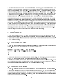
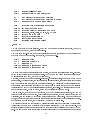
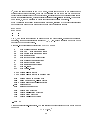
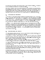
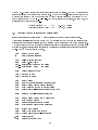
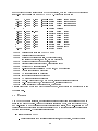
The gure below indicates the data ows resulting from user commands described in the remainder
of this manual.
XFOIL 6.9 Data Flow
Disk file
Airfoil x,y
coordinate file
NACA
LOAD
Stored
Data
SAVE
ROUTine
COMMand
INTE
Polars
PCOP
OPER
PANE
Buffer
Airfoil
EXEC
ASET
Current
Airfoil
GSET
PACC
ALFA,
ASEQ,
CL...
MODI,
CAMB,
...
QSET
3
Qspec
QSET
MODI
MODI
MDES
QDES
Q(s)
Polar save file
CL,CD...
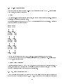
XFOIL is simply executed with:
% xfoil
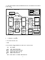
When the program starts, the following top level menu and prompt appear:
.OPER
.MDES
.QDES
.GDES
PWRT
EXEC
Program Execution
QUIT
1: CL,CD...
2: CL,CD...
.
.
PGET
GDES
EXEC
1: x, y
2: x, y
.
.
Exit program
Direct operating point(s)
Complex mapping design routine
Surface speed design routine
Geometry design routine
SAVE f Write airfoil to labeled coordinate file
7
PSAV f Write airfoil to plain coordinate file
ISAV f Write airfoil to ISES coordinate file
MSAV f Write airfoil to MSES coordinate file
REVE Reverse written-airfoil node ordering
LOAD f Read buffer airfoil from coordinate file
NACA i Set NACA 4,5-digit airfoil and buffer airfoil
INTE Set buffer airfoil by interpolating two airfoils
NORM Buffer airfoil normalization toggle
BEND Display structural properties of current airfoil
XYCM rr Change CM reference location, currently 0.25000 0.00000
PCOP
PANE
.PPAR
Set current-airfoil panel nodes directly from buffer airfoil points
Set current-airfoil panel nodes ( 140 ) based on curvature
Show/change paneling
.PLOP
Plotting options
WDEF f Write current-settings file
RDEF f Reread current-settings file
NAME s Specify new airfoil name
NINC Increment name version number
Z
U
XFOIL
Zoom
| (available in all menus)
Unzoom |
c>
The commands preceded by a period place the user in another lower-level menu. The other commands are executed immediately and the user is prompted for another top level command. The
lowercase letters i,r,f,s following some commands indicate the type of argument(s) expected by
the command:
i integer
r real
f lename
s character string
Commands will be shown here in uppercase, although they are not case sensitive.
Typically, either the LOAD or the NACA command is issued rst to create an airfoil for analysis or
redesign. The NACA command expects an integer argument designating the airfoil:
XFOIL c> NACA 4415
As with all commands, omitting the argument will produce a prompt:
XFOIL c> NACA
Enter NACA 4 or 5-digit airfoil designation
8
i> 4415
The LOAD command reads and processes a formatted airfoil coordinate le dening an arbitrary
airfoil. It expects a lename argument:
XFOIL c> LOAD e387.dat
The NACA or LOAD commands can be skipped if XFOIL is executed with a lename as an argument,
as for example
% xfoil e387.dat
which then executes the LOAD procedure before the rst menu prompt is given.
3.1 Airfoil le formats
recognizes four le formats: Plain, Labeled, ISES, MSES. All data lines are signicant with
the exception of lines beginning with \#", which are ignored.
LOAD
3.1.1 Plain coordinate le
This contains only the x; y coordinates, which run from the trailing edge, round the leading edge,
back to the trailing edge in either direction:
X(1) Y(1)
X(2) Y(2)
.
.
.
.
X(N) Y(N)
3.1.2 Labeled coordinate le
This is the same as the plain le, except that it also has an airfoil name string on the rst line:
NACA 0012
X(1) Y(1)
X(2) Y(2)
.
.
This is deemed the most convenient format to use. The presence of the name string is automatically
recognized if it does not begin with a Fortran-readable pair of numbers. Hence, \00 12 NACA
Airfoil" cannot be used as a name, since the \00 12" will be interpreted as the rst pair of
coordinates. \0012 NACA" is OK, however.
Some Fortran implementations will also choke on airfoil names that begin with T or F. These will
be interpreted as logical variables, defeating the name-detection logic. Beginning the name with T
or F is a workable solution to this "feature".
9
3.1.3 ISES coordinate le
This has four or ve ISES grid domain parameters in addition to the name:
NACA
-2.0
X(1)
X(2)
.
0012
3.0 -2.5 3.0
Y(1)
Y(2)
.
If the second line has four or more numbers, then these are interpreted as the grid domain parameters.
3.1.4 MSES coordinate le
This is the same as the ISES coordinate le, except that it can contain multiple elements, each one
separated by the line
999.0 999.0
The user is asked which of these elements is to be read in.
3.2 Buer airfoil normalization
XFOIL will normally perform all operations on an airfoil with the same shape and location in
cartesian space as the input airfoil. However, if the normalization ag is set (toggled with the
NORM command), the buer airfoil coordinates will be immediately normalized to unit chord and
the leading edge will be placed at the origin. A message is printed to remind the user.
3.3 Buer airfoil generation via interpolation
The INTE command is new in XFOIL 6.9, and allows interpolating or "blending" of airfoils in various
proportions. The polar shape of an interpolated airfoil will often be quite close to the interpolated
polars of its two parent airfoils. Extrapolation can also be done by specifying a blending fraction
outside the 0..1 range, although the resulting airfoil may be quite weird if the extrapolation is
excessive.
A good way to use INTE is to "augment" or "tone down" the modications to an airfoil performed
in MDES or GDES. For example, say airfoil B is obtained by modifying airfoil A:
A ! MDES ! B
Suppose the modication changed A's polar in the right direction, but not quite far enough. The
additional needed change can be done by extrapolating past airfoil B in INTE:
Airfoil "0": A
Airfoil "1": B
Interpolating fraction 0..1 :
Output airfoil: C
1.4
10
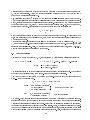
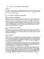
Plotted along the "modication axis", the airfoils are:
A
0.0
B
1.0
C
1.4 ...
So airfoil C has 40% more of the change received by B in the redesign. Airfoil C's polar will also
be changed about 40% more as intended.
3.4 Further buer airfoil manipulation
The GDES facility allows very extensive manipulation of the buer airfoil. This will be described
in much more detail in a later section. If only analysis is performed, the GDES facility would not
normally be used.
3.5 Generation of current airfoil
When the buer airfoil coordinates are read from a le during startup, or read in via the LOAD
command, they are by default also copied directly into the \current", or working airfoil. Hence,
no special action is needed to start analysis operations. However, if the starting buer airfoil has a
poor point distribution (too many, too few, poorly spaced, etc), one can use PANE to create a better
panel node distribution for the current airfoil on the splined buer airfoil shape. The paneling
routine increases the point density in areas of high curvature (i.e. the leading edge) and at the
trailing edge to a degree specied by the user. The user can also increase panel density over one
additional interval on each airfoil side, perhaps near transition. The current-airfoil paneling can be
displayed and/or modied with PPAR.
In some cases it is desirable to explicitly re-copy the buer airfoil into the current airfoil via PCOP.
In previous XFOIL versions this had to be done with the equivalent command sequence
LOAD
GDES
EXEC
With XFOIL 6.9, the GDES, EXEC commands after LOAD are now superuous.
The NACA command automatically invokes the paneling routine to create a current airfoil with a
suitable paneling.
3.6 Saving airfoil coordinates
A coordinate le in any one of these four formats can be written with the PSAV, SAVE, ISAV, or MSAV
command, respectively. When issuing the MSAV command, the user is also asked which element in
the le is to be overwritten. XFOIL can thus be used to easily "edit" individual elements in MSES
multielement congurations. Of course, normalization should not be performed on an element if
it is to be written back to the same multielement le. Only the current-airfoil coordinates can be
saved to a le. If the buer or polar x; y coordinates need to be saved, they must rst be copied
into the current airfoil.
11
4
Units
Most XFOIL operations are performed on the airfoil's cartesian coordinates x; y , which do not
necessarily have a unit chord c. Since the chord is ambiguous for odd shapes, the XFOIL force coeÆcients CL, CD , CM are obtained by normalizing the forces and moment with only the freestream
dynamic pressure (the reference chord is assumed to be unity). Likewise, the XFOIL Reynolds
number RE is dened with the freestream velocity and viscosity, and an implied unit chord:
CL = L=q
V = freestream speed
CD = D=q
= freestream kinematic viscosity
CM = M=q
= freestream density
RE = V=
q = 0:5 V
The conventional denitions are
Cl = L=qc
Cd = D=qc
Cm = M=qc
Rec = V c=
so that the conventional and XFOIL denitions dier only by the chord factor c or c .
For example, a NACA 4412 airfoil is operated in the OPER menu at
RE = 500000
= 3Æ
rst with c = 1:0, and then with c = 0:5 (changed with SCAL command in the GDES menu, say).
The results produced by XFOIL are:
c = 1:0 : CL = 0:80 CD = 0:0082 (RE = 500000; Rec = 500000)
c = 0:5 : CL = 0:40 CD = 0:0053 (RE = 500000; Rec = 250000)
Since CL is not normalized with the chord, it is nearly proportional to the airfoil size. It is not
exactly proportional, since the true chord Reynolds number Rec is dierent, and there is always
a weak Reynolds number eect on lift. In contrast, the CD for the smaller airfoil is signicantly
greater than 1/2 times the larger-airfoil CD , since chord Reynolds number has a signicant impact
on prole drag. Repeating the c = 0:5 case at RE = 1000000, produces the expected result that
CL and CD are exactly 1/2 times their c = 1:0 values.
2
2
2
c = 0:5
: CL = 0:40 CD = 0:0041 (RE = 1000000; Rec = 500000)
Although XFOIL performs its operations with no regard to the size of the airfoil, some quantities
are nevertheless dened in terms of the chord length. Examples are the camber line shape and BL
trip locations, which are specied in terms of the relative x=c; y=c along and normal to the airfoil
chord line. This is done only for the user's convenience. In the input and output labeling, "x,y"
always refer to the cartesian coordinates, while "x/c, y/c" refer to the chord- based coordinates
which are shifted, rotated, and scaled so that the airfoil's leading edge is at (x=c; y=c) = (0; 0), and
the airfoil's trailing edge is at (x=c; y=c) = (1; 0). The two systems cooincide only if the airfoil is
normalized.
5
Analysis Routine (OPER)
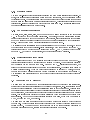
Issuing the OPER command will produce the prompt
12
.OPERi c>
Typing a "?" will result in the full OPER analysis menu being displayed:
<cr>
!
Visc
.VPAR
Re
Mach
Type
ITER
INIT
Return to Top Level
Redo last ALFA,CLI,CL,ASEQ,CSEQ,VELS
r
r
r
i
Toggle
Change
Change
Change
Change
Change
Toggle
Inviscid/Viscous mode
BL parameter(s)
Reynolds number
Mach number
type of Mach,Re variation with CL
viscous-solution iteration limit
BL initialization flag
Alfa
CLI
Cl
ASeq
CSeq
r
r
r
rrr
rrr
Prescribe
Prescribe
Prescribe
Prescribe
Prescribe
SEQP
CINC
HINC
Pacc
PGET
PWRT
PSUM
PLIS
PDEL
PSOR
PPlo
APlo
ASET
PREM
PPAX
Toggle polar/Cp(x) sequence plot display
Toggle minimum Cp inclusion in polar
Toggle hinge moment inclusion in polar
i Toggle auto point accumulation to active polar
f Read new polar from save file
i Write polar to save file
Show summary of stored polars
i List stored polar(s)
i Delete stored polar
i Sort stored polar
ii. Plot stored polar(s)
ii. Plot stored airfoil(s) for each polar
i Copy stored airfoil into current airfoil
ir. Remove point(s) from stored polar
Change polar plot axis limits
alpha
inviscid CL
CL
a sequence of alphas
a sequence of CLs
RGET f
RDEL i
Read new reference polar from file
Delete stored reference polar
GRID
CREF
FREF
Toggle Cp vs x grid overlay
Toggle reference Cp data overlay
Toggle reference CL,CD.. data display
CPx
CPV
.VPlo
.ANNO
HARD
Plot Cp vs x
Plot airfoil with pressure vectors (gee wiz)
BL variable plots
Annotate current plot
Hardcopy current plot
13
SIZE r
CPMI r
Change plot-object size
Change minimum Cp axis annotation
BL i
BLC
BLWT r
Plot boundary layer velocity profiles
Plot boundary layer velocity profiles at cursor
Change velocity profile scale weight
FMOM
FNEW
VELS
DUMP
CPWR
CPMN
NAME
NINC
Calculate flap hinge moment and forces
Set new flap hinge point
Calculate velocity components at a point
Output Ue,Dstar,Theta,Cf vs s,x,y to file
Output x vs Cp to file
Report minimum surface Cp
Specify new airfoil name
Increment name version number
rr
rr
f
f
s
.OPERi c>
The commands are not case sensitive. Some commands expect multiple arguments, but if the
arguments are not typed, prompts will be issued.
The most commonly-used commands have alternative short forms, indicated by the uppercase part
of the command in the menu list. For example, the menu shows...
Alfa
CLI
Cl
ASeq
CSeq
r
r
r
rrr
rrr
Prescribe
Prescribe
Prescribe
Prescribe
Prescribe
alpha
inviscid CL
CL
a sequence of alphas
a sequence of CLs
The A command is the short alternative form of ALFA, and C is the short alternative of CL. Likewise,
AS and CS are the short forms of ASEQ and CSEQ. The CLI command has no short form (as indicated
by all capitals in the menu), and must be fully typed.
Hopefully, most of the commands are self-explanatory. For inviscid cases, the CLI and CL commands
are identical. For viscous cases, CLI is equivalent to specifying alpha, this being determined a priori
from the specied lift coeÆcient via an inviscid solution. CL will return a viscous solution with
the specied true viscous lift coeÆcient at an alpha which is determined as part of the solution
(prescribing a CL above CL will cause serious problems, however!). The user is always prompted
for any required input. When in doubt, typing a "?" will always produce a menu.
After an ALFA, CL, or CLI command is executed, the Cp vs x distribution is displayed, and can be
displayed again at any time with CPX. If the viscous mode is active, the true viscous Cp is shown as
a solid line, and the inviscid Cp at that same alpha is shown as a dashed line. Each dash covers one
panel, so the local dashed line density is also a useful visual indicator of panel resolution quality.
If the inviscid mode is active, only the inviscid Cp is shown as a solid line.
The dierence between the true viscous Cp distribution (solid line) and the inviscid Cp distribution
(dashed line) is due to the modication of the eective airfoil shape by the boundary layers. This
eective airfoil shape is shown superimposed on the actual current airfoil shape under the Cp vs x
plot. The gap between these eective and actual shapes is equal to the local displacement thickness
max
14
Æ ,
which can also be plotted in the VPAR menu. This is only about 1/3 to 1/2 as large as the
overall boundary layer thickness, which can be visualized via the BL or BLC commands which
diplay velocity proles through the boundary layer. BL displays a number of proles equally spaced
around the airfoil's perimeter, while BLC displays proles at cursor-selected locations. The zooming
commands Z, U, may be necessary to better see these small proles in most cases.
If the Cp reference data overlay option is enabled with CREF, initiating a Cp vs x plot will rst result
in the user being prompted for a formatted data le with the following format:
x(1) Cp(1)
x(2) Cp(2)
.
.
.
.
The Cp vs x plot is then displayed as usual but with the data overlaid. If FREF has been issued
previously, then numerical reference values for CL , CD , etc. will be requested and added to the
plot next to the computed values.
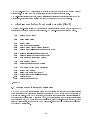
Boundary-layer quantities are plotted from the VPLO menu:
H
DT
DB
UE
CF
CD
N
CT
RT
RTL
Plot
Plot
Plot
Plot
Plot
Plot
Plot
Plot
Plot
Plot
kinematic shape parameter
top
side Dstar and Theta
bottom side Dstar and Theta
edge velocity
skin friction coefficient
dissipation coefficient
amplification ratio
max shear coefficient
Re_theta
log(Re_theta)
X rrr Change x-axis limits
Y rrr Change y-axis limits on current plot
Blow Cursor blowup of current plot
Rese Reset to default x,y-axis limits
SIZE r Change absolute plot-object size
.ANNO Annotate plot
HARD Hardcopy current plot
GRID
SYMB
LABE
CLIP
Toggle
Toggle
Toggle
Toggle
grid plotting
node-symbol plotting
label plotting
line-plot clipping
..VPLO c>
This menu is largely self-explanatory. The skin friction coeÆcient plotted with the CF command is
dened as
Cf = =0:5V1
2
15
This diers from the standard boundary layer theory denition which uses the local Ue rather than
V1 for the normalization. Using the constant freestream reference makes Cf (x) have the same
shape as the physical shear stress (x).
The dissipation coeÆcient CD0 (this is NOT the drag coeÆcient!!!) is plotted with the CD command.
CD0 (x) is proportional to the local energy dissipation rate due to viscous shear and turbulent mixing.
Hence, it indicates where on the airfoil drag is being created. It is in fact a much better indicator of
drag production than Cf (x), since Cf does not account for pressure drag. CD0 , on the other hand,
accounts for everything. Its relationship to the total prole drag coeÆcient is simply
1 0
CD =
2 CD ds
Z
0
with the integration performed over both boundary layers and also the wake. It will be seen that
if the ow is separated at the trailing edge, much of the drag contribution (energy dissipation) of
CD0 occurs in the wake.
As mentioned earlier, all forces are normalized with freestream dynamic pressure only. CL, CD ,
CM are the usual chord-based denitions only if the airfoil has a unit chord { in general, they will
scale with the airfoil's chord. Also, CM is dened about the cartesian point (x ; y ) = (0.25,0.0),
which is not necessarily the airfoil's 1/4 chord point.
ref
ref
5.1 Force calculation
The lift and moment coeÆcients CL, CM , are calculated by direct surface pressure integration:
CL = L=q = Cp dx
CM = M=q =
Cp [(x x ) dx + (y y ) dy]
I
I
ref
where
x
y
ref
= x cos() + y sin()
= y cos() x sin()
The integrals performed in the counterclockwise direction around the airfoil contour. The pressure
coeÆcient Cp is calculated using the Karman-Tsien compressibility correction.
The drag coeÆcient CD is obtained by applying the Squire-Young formula at the last point in the
wake | at the trailing edge.
CD = D=q = 2 1 = 2 (u=V ) H =
where = momentum thickness
u = edge velocity
at end of computed wake
H = shape parameter
and 1 = momentum thickness
very far downstream
V = freestream velocity
The Squire-Young formula in eect extrapolates the momentum thickness to downstream innity.
It assumes that the wake behaves in a asymptotic manner downstream of the point of application.
This assumption is strongly violated in the near-wake behind an airfoil with trailing edge separation,
but is always reasonable some distance behind the airfoil. Hence, the usual application of SquireYoung at the trailing edge is questionable with separation present, but its application at the last
wake point (typically 1 chord downstream) is always reasonable. Also, application at the last wake
not
(
9
>
=
>
;
)
16
+5) 2
point also results in the formula having a smaller eect in any case, since there u ' V , and hence
1 ' .
In most 2-D airfoil experiments, drag is measured indirectly by measuring 2=c in the wake, often
within one chord of the airfoil's trailing edge. For consistency, this should be compared to the
Theta value predicted by XFOIL at the same wake location, rather than the "true" Cd = 21=c
value which is eectively at downstream innity. In general, 1 will be smaller than . In most
airfoil drag measurement experiments, this dierence may amount to the drag measurement being
several percent too large, unless some correction is performed.
In addition to calculating the total viscous CD from the wake momentum thickness, XFOIL also
determines the friction and pressure drag components CD , CD of this total CD . These are
calculated by
CD = Cf dx
CD = CD CD
Here, Cf is the skin friction coeÆcient dened with the freestream dynamic pressure, not the BL
edge dynamic pressure commonly used in BL theory. Note that CD is deduced from CD and CD
instead of being calculated via surface pressure integration. This conventional denition
CD = Cp dy
f
p
I
p
f
f
p
f
I
p
is
not
used, since it is typically swamped by numerical noise.
5.2 Transition criterion
Transition in an XFOIL solution is triggered by one of two ways:
free transition: en criterion is met
forced transition: a trip or the trailing edge is encountered
n
The e method is always active, and free transition can occur upstream of the trip. The en method
has the user-specied parameter n , which is the log of the amplication factor of the mostamplied frequency which triggers transition. A suitable value of this parameter depends on the
ambient disturbance level in which the airfoil operates, and mimics the eect of such disturbances
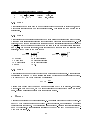
on transition. Below are typical values of n for various situations.
Situation
n
sailplane
12{14
motorglider
11{13
clean wind tunnel 10{12
average wind tunnel 9
dirty wind tunnel 4{8
The choice n = 9 corresponds to the \standard" e method, and is the most common choice.
It must be pointed out that the en method in XFOIL is actually the simplied envelope version,
which is the same as the full en method only for ows with constant H (x). If H is not constant,
the two methods dier somewhat, but this dierence is typically within the uncertainty in choosing
n .
The en method is only appropriate for predicting transition in situations where the growth of 2-D
Tollmien-Schlichting waves via linear instability is the dominant transition-initiating mechanism.
Fortunately, this happens to be the case in a vast majority of airfoil applications. Other possible
mechanisms are:
crit
crit
crit
9
crit
crit
17
Crossow instabilities. These occur on swept wings with signicant favorable chordwise pres-
sure gradients.
Attachment-line transition. This requires large sweep, large LE radius, and a large Reynolds
number. Occurs primarily on big jets.
Bypass transition. This occurs in cases with suÆcient wall roughness and/or large freestream
turbulence or vibration levels. The linear-instability phase predicted by the en method is
"bypassed", giving relatively early transition. Usually occurs in favorable pressure gradients,
while the linear-instability mechanism usually dominates in adverse pressure gradients.
If any of these alternative transition mechanisms are present, the trips must be set to mimick their
eect. The bypass transition mechanism can be mimicked to some extent by the en method by
setting n to a small value | n = 1 or less. This will cause transition just after linear instability
begins. For very large freestream turbulence or roughness in favorable pressure gradients, bypass
transition can occur before the linear instability threshold, and in this case trips will have to be set
as well.
crit
crit
5.3 Numerical accuracy
5.3.1 Panel density requirements
If strong separation bubbles are present in a viscous solution, then it is very important to have
good panel resolution in the region of the bubble(s). The large gradients at a bubble tend to
cause signicant numerical errors even if a large number of panels is used. If a separation bubble
appears to be poorly resolved, it is a good idea to re-panel the airfoil with more points, and/or
with points bunched around the bubble region. The paneling is controlled from the PPAR menu.
A good rule of thumb is that the shape parameter Hk just after transition in the bubble should not
decrease by more than 1.0 per point. Likewise, the surface velocity Ue=V1 should not change by
more than 0.05 per point past transition, otherwise there may be signicant numerical errors in the
drag. The point values can be observed by issuing SYMB from the VPLO menu. Moderate chord
Reynolds numbers (1{3 million, say) usually require the nest paneling, since the bubbles are still
important, but very small. On many airfoils, especially those with small leading edge radii, the
development of the small bubble which forms just behind the leading edge can have a signicant
eect on CL . For such cases, the default paneling density at the bubble may not be adequate.
In all cases, inadequate bubble resolution results in a "ragged" or "scalloped" CL vs CD drag polar
curve, so fortunately this is easy to spot.
max
5.3.2 Dierencing order of accuracy
The BL equations are normally discretized with two-point central dierencing (i.e. the Trapezoidal
Scheme), which is second-order accurate, but only marginally stable. In particular, it has problems
with the relatively sti shape parameter and lag equations at transition, where at high Reynolds
number the shape parameter must change very rapidly. Oscillations and overshoots in the shape
parameter will occur with the Trapezoidal Scheme if the grid cannot resolve this rapid change. To
avoid this nasty behavior, upwinding must be introduced, resulting in the Backward Euler Scheme,
which is very stable, but has only rst-order accuracy. Previous versions of XFOIL allowed a specic
constant amount of upwinding to be user-specied. Currently, XFOIL automatically introduces
18
upwinding into the equations only in regions of rapid change (typically transition). This ensures
that the overall scheme is stable and as accurate as possible.
Since only a minimal amount of upwinding is introduced in the interest of numerical accuracy,
small oscillations in the shape parameter H will sometimes appear near the stagnation point if
relatively coarse paneling is used there. These oscillations are primarily a cosmetic defect, and do
not signicantly aect the downstream development of the boundary layer. Eliminating them by
increasing upwiding would in fact produce much greater errors in the overall viscous solution.
5.4 Viscous solution acceleration
The execution of a viscous case requires the solution of a large linear system every Newton iteration. The coeÆcient matrix of this system is 1/3 full, although most of its entries are very small.
Substantial savings in CPU time (factor of 4 or more) result when these small entries are neglected.
SUBROUTINE BLSOLV which solves the large Newton system ignores any o-diagonal element
whose magnitude is smaller than the variable VACCEL, which is initialized in SUBROUTINE
INIT, and which can be changed at runtime from the VPAR menu with the VACC command.
A nonzero VACCEL parameter should in principle degrade the convergence rate of the viscous
solution and thus result in more Newton iterations, although the eect is usually too small to notice.
For very low Reynolds number cases (less than 100000), it
adversely aect the convergence
rate or stability, and one should try reducing VACCEL or even setting it to zero if all other eorts at
convergence are unsuccessful. The value of VACCEL has absolutely no eect on the nal converged
viscous solution (if attained).
may
5.5 Polar calculations and plotting
The polar calculation facility driven from the OPER menu deserves a detailed description. It has
been considerably upgraded from previous XFOIL versions.
The simplest way to create a polar is to issue the PACC command which sets the auto polar accumulation toggle and asks for the optional save and dump lenames. If either lename is given,
each computed operating point will be stored internally and also written to the specied le. If no
lename is given, the automatic writing is not performed.
The polar's operating points can be computed individually with ALFA, or more conveniently en
masse with ASEQ. One can also use CL or CSEQ, although these will not work close to CL .
The polar can be plotted anytime with PPLO. If previous polars have been computed or read in
with PGET, they can be plotted as well. If a polar is deemed incomplete, additional points can be
computed as needed.
If automatic writing of a polar was not chosen (no lename was given for PACC), the polar can be
written later all at once with the PWRT command. The only drawback to this approach is that if
the program crashes during a polar calculation sweep for whatever reason, the computed polar and
all other stored information will be lost.
If existing lenames are given to PACC, the subsequent computed points will be appended to these
les, but only if the airfoil name and ow parameters in the le match the current parameters.
This is to prevent clobbering of the polar le with "wrong" additional points. Messages are always
produced informing the user of what's going on.
max
19
5.6 O-line polar plotting
Polar save le(s) can also be plotted o-line with the separate program PPLOT. This is entirely
menu driven, and is simply executed:
% pplot
The le pplot.def contains plotting parameters, and is read automatically if available. If it's not
available, then internal defaults are used.
Like the RGET,FREF commands in OPER, PPLOT permits reference data to be overlaid. A reference
polar data le has the following form:
CD(1) CL(1)
CD(2) CL(2)
.
.
.
.
999.0 999.0
alpha(1) CL(1)
alpha(2) CL(2)
.
.
.
.
999.0 999.0
alpha(1) Cm(1)
alpha(2) Cm(2)
.
.
.
.
999.0 999.0
Xtr/c(1) CL(1)
Xtr/c(2) CL(2)
.
.
.
.
999.0 999.0
The number of points in each set (CD-CL, alpha-CL, etc.) is arbitrary, and can be zero.
The contents of a polar dump le can be selectively plotted with the separate menu-driven program
PXPLOT. It is executed with:
% pxplot <dump filename>
This allows surface plots of Cp vs x, H vs x, etc. for any or all of the saved operating points. Of
course, these plots can be generated in XFOIL for any individual operating point, so PXPLOT and
the dump le itself are somewhat redundant in this respect.
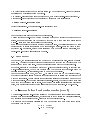
5.7 Re, Mach dependence on CL
A few comments are in order on the TYPE command, which allows the user to set the dependence
of the Mach and Reynolds numbers on CL. Any CL{CD polar can be of the following three types:
20
Type parameters held constant varying
xed
1
M
,
RE
lift
chord,
velocity
p
p
2
M CL , RE CL
velocity chord, lift
3
M , RE CL
chord lift , velocity
5.7.1 Type 1
This corresponds to a given wing at a xed velocity going over an angle of attack range, as in a
wind tunnel test alpha sweep or a sudden aircraft pullup. This is also the common form for an
airfoil polar.
5.7.2 Type 2
This corresponds to an aircraft in level ight at a given altitude undergoing trim speed changes.
This is the most useful airfoil polar form for determining a drag polar for an aircraft at 1{g. For
thispcase, The "Mach number" input with the MACH command is actually interpreted as the product
M CLp, and the "Reynolds number" input with the VISC or RE commands is actually interpreted
as RE CL. For a wing in level ight, these products can be computed from the following exact
relations, with RE based on the mean chord:
2
W=S =
1 2W =
M CL =
RE CL =
p
W = weight
S = wing area
AR = aspect ratio
b = span
1 2
p
p
p = ambient pressure
= kinematic viscosity
= ambient air density
= 1.4
1 2
AR
5.7.3 Type 3
This corresponds to a wing of "rubber chord" with a given lift at a given speed. This is best used
for selecting an optimum CL for an airfoil while taking Reynolds number changes into account.
The product RE CL can be computed from the following:
2W
RE CL =
V b
Caution must be used with Types 2 and 3 so as to not allow the CL to go negative. In addition,
with non-zero Mach and Type 2, the CL must not fall below that value which makes Mach exceed
unity. Warning messages are printed when these problems occur.
6
Output
All output goes directly to the terminal screen. H. Youngren's plot package Xplot11 (libPlt.a)
used by XFOIL drives monochrome and color X-Windows graphics, and generates B&W or color
PostScript les for hardcopy. The default setup assumes color X-Windows graphics (if available),
and B&W PostScript. These defaults are controlled by the IDEV and IDEVRP ags in SUBROUTINE INIT (in xfoil.f).
21
The Xplot11 library should work on all Unix systems. The Makele in the ./plotlib/ directory
requires some modications for some machines.
The default X-graphics window is in Landscape mode, with a black (reverse-video) background. A
white (normal-video) background can be selected by setting the Unix shell variable
% setenv XPLOT11_BACKGROUND white
before Xfoil is started. The nicer reverse-video is restored with:
% unsetenv XPLOT11_BACKGROUND
See the plotlib/Doc le for more info on the plot library.
Xplot11 provides a built-in Zoom/Unzoom capability which can be applied to whatever is on the
screen. Zooming/Unzooming can be perfomed with the Z and U commands from nearly all the
menus | these commands are not listed to reduce clutter.
Some of the menus also have their own Blowup/Reset commands. The distinction is that XFOIL's
plots don't try to adjust themselves to Zoom parameters, so a highly-"Zoomed" plot may show
nothing at all. In contrast, Blowup/Reset instructs XFOIL to change its own plot scales, so a
highly-"Blown-up" plot will at least show the axes.
6.1 Plot Hardcopy
For hardcopy, the current screen plot can be echoed to a PostScript le plot.ps with the HARD
command. The size of the plot objects on the screen and on hardcopy can be changed with the
SIZE command from most menus. The number requested is the width of the plot in inches.
If the plot.ps le is to be previewed with some X-Windows PostScript viewer, or imported into
word-processing systems, XFOIL must be exited with QUIT in order for the plot.ps le to be
properly terminated. For just printing, this may or may not be necessary.
For the geometry plot in GDES, and the Q (s) plots in QDES and MDES (described below),
the hardcopy plot size will also be aected if the graphics window is resized with the cursor at the
window manager level. This is because the plot is always scaled so that it lls up as much of the
window as possible. If the window size is left at its start-up size, the hardcopy plot widths will
come out with the specied size in inches. If any window dimension is increased from its default
value, then a subsequent hardcopy plot will probably not t on a standard 8.5" x 11.0" sheet.
spec
7
Full-Inverse Surface Speed Design Routine (MDES)
XFOIL's Full-Inverse complex-mapping facility MDES takes as input a speed distribution "Q "
specied over the entire airfoil surface, modies it somewhat to satisfy the Lighthill constraints,
and generates a new overall geometry. First a bit of the underlying theory...
The geometry and the surface velocities can both be computed from a set of complex mapping
coeÆcients Cn in the form
x + iy = z (!; Cn )
u iv = w(!; Cn ; )
spec
22
where ! = 0::2 is the independent parameter going around the airfoil. The z and w functions are
rather complicated but this is not important here. The key to the full-inverse method is that the
mapping coeÆcients Cn can be computed from a known contour angle (!) = arctan(dy=dz) OR
from a surface speed Q(!) = ju ivj = jwj. The other quantity then follows. In summary, the
operations and their commands are...
a) Direct problem: ! Cn ! u iv; Q (QSET)
b) Inverse problem: Q ! Cn ! x + iy; (EXEC)
spec
7.1 Creation of seed surface speed distribution
performs QSET and sets Q = Q automatically upon entry if Q does not exist.
This default initialization in eect makes MDES a redesign method in which the surface speed
distribution of an existing airfoil is used as a starting point to generate a new speed distribution.
A \pure" design code which requests the entire surface speed distribution every time is often less
natural to use, since airfoil design is invariably an iterative process involving repeated analyze/x
cycles. The MDES menu is shown below.
MDES
spec
spec
<cr>
!
Return to Top Level
Redo previous command
INIT
QSET
AQ r..
CQ r..
Re-initialize mapping
Reset Q_spec <== Q
Show/select alpha(s) for Qspec
Show/select CL(s) for Qspec
Symm Toggle symmetry flag
TGAP r Set new TE gap
TANG r Set new TE angle
Modi
MARK
SMOO
FILT
SLOP
Modify Qspec
Mark off target segment for smoothing
Smooth Qspec inside target segment
Apply Hanning filter to entire Qspec
Toggle modified-Qspec slope matching flag
eXec
Execute full-inverse calculation
Plot
VISC
REFL
SPEC
Replot Qspec (line) and Q (symbols)
Qvis overlay toggle
Reflected Qspec overlay toggle
Plot mapping coefficient spectrum
Blow Blowup plot region
Rese Reset plot scale and origin
SIZE r Change absolute plot-object size
.ANNO Annotate plot
HARD Hardcopy current plot
23
PERT
Perturb one Cn and generate perturbed geometry
.MDES c>
As described above, the initial Q distribution is taken from Q, the speed distribution corresponding to the current geometry at the last angle of attack employed in OPER. Q can be set
back to this Q with QSET anytime.
spec
spec
7.2 Modication of surface speed distributions
7.2.1 Cursor input of modications
Qspec can be modied to whatever is desired with the MODI command by specifying points with the
screen cursor which are then splined. The points can be entered in any order. The previously-input
points can be erased one by one by clicking on the "Erase" button or simply typing e in the
graphics window. The input sequence is terminated by clicking on the "Done" button or by typing
d in the graphics window. The "Abort" button or typing a aborts the MODI command and returns
to the MDES menu. The BLOW command can be used to enlarge regions of interest at any time by
specifying opposite corners of the blowup region.
7.2.2 Modication endpoint blending
Normally, the modied piece of Q (s) is blended into the current Q (s) with matching slopes
at the piece endpoints. This slope matching can be turned on/o with the SLOP toggle command.
If slope matching is turned o, the modied piece will match only the existing value, but a slope
discontinuity will be allowed.
spec
spec
7.2.3 Smoothing
Qspec can be smoothed with the SMOO command, which normally operates on the entire distribution,
but can be conned to a target segment whose endpoints are selected with the MARK command.
The smoothing acts to alleviate second derivatives in Q (s), so that with many consecutive SMOO
commands Q (s) will approach a straight line over the target segment. If the slope-matching
ag is set, the endpoint slopes are preserved.
The FILT command is an alternative smoothing procedure which acts on the Fourier coeÆcients of
Q directly, and is global in its eect. It is useful for "cleaning up" the entire Q (s) distribution
if noise is present from some geometric glitch on the airfoil surface. Also, unintended noise might
be introduced into Q from a poor modication via the cursor.
FILT acts by multiplying the Fourier coeÆcients by a Hanning window lter function raised to the
power of a lter parameter F . This tapers o the high frequencies of Q to varying degrees. A
value of F = 0:0 gives no ltering, F = 1:0 gives the standard Hanning lter, F = 2:0 applies the
Hanning lter twice, etc. The standard Hanning lter appears to be a bit too drastic, so a lter
parameter of F = 0:2 is currently used. Hence, issuing FILT ve times corresponds to the standard
Hanning lter. The SPEC command displays the mapping coeÆcient spectrum at any time.
spec
spec
spec
spec
spec
spec
24
7.2.4 Symmetry forcing
The symmetry-forcing option (SYMM toggle) is useful when a symmetric airfoil is being designed. If
active, this option zeroes out all antisymmetric (camber) Q changes, and doubles all symmetric
(thickness) changes. This unfortunately has the annoying side eect of also doubling the numerical
roundo noise in Q every time a MODI operation is performed. This noise sooner or later becomes
visible as high-frequency wiggles which double with each MODI command. Occasionally issuing FILT
keeps this parasitic noise growth under control.
spec
spec
7.2.5 New geometry computation
The MODI, BLOW, MARK, SMOO, SLOP, FILT commands can be issued repeatedly in any order until
Q
is modied to have the desired distribution. In general, the speed distributions actually
plotted will not exactly match what was input with the cursor, since corrections are automatically
added to maintain the specied trailing edge gap and to enforce consistency with the freestream
speed. These are known as the Lighthill constraints on the surface speed.
The trailing edge gap is initialized from the initial airfoil and can be changed with TGAP. To reduce
the "corrupting" eect of the constraint-driven corrections, a good rule of thumb is that the Q
distribution should be modied so as to preserve the total CL. The CL is simply twice the area
under the Q (s) curve (= 2 x circulation), so that this area should be preserved.
spec
spec
spec
7.2.6 Multipoint surface speed display
A very useful feature of the MDES facility is the ability to display and modify a number of Q
distributions corresponding to dierent alpha or inviscid CL values. These values are displayed
and/or selected via the AQ or CQ commands. When any one Q distribution is modied, the
result of modication is also displayed on all the other distributions. This allows rapid design at
multiple operating points. When the Q curves correspond to specied CL values, the alpha
for each curve will be adjusted after each Q modication so as to preserve that curve's CL.
The resulting Q will therefore not match the input cursor points exactly because of this alpha
correction.
spec
spec
spec
spec
spec
7.3 Generation of new geometry
The EXEC command generates a new buer airfoil corresponding to the current Q distribution.
If subsequent operations on this airfoil are to be performed (SAVE, OPER, etc.), it is necessary to rst
generate a current airfoil from this buer airfoil using PANE at the top level menu. This seemingly
complicated sequence is necessary because the airfoil points generated by EXEC are uniformly spaced
in the circle plane, which gives a rather poor point (panel node) spacing distribution on the physical
airfoil. This sequence also prevents the current airfoil from being overwritten immediately when
EXEC is issued. Once the new current airfoil is generated with PANE, it can then be analyzed in
OPER, modied in GDES, or whatever.
The PERT command allows manual input of the complex mapping coeÆcients Cn which determine
the geometry. These coeÆcients are normally determined from Q (s) (this is the essence of the
inverse method). The PERT command is provided simply as a means of allowing generation of
geometric perturbation modes, possibly for external optimization or whatever.
spec
spec
25
The manually-changed Cn values result in changes in geometry as well as the current Q (s)
distributions. The QSET command will restore everything to its unperturbed state.
The Full-Inverse facility is very fast, after an initialization calculation of several seconds (on a RISC
workstation), it requires only a fraction of a second to generate the new buer airfoil.
spec
8
Mixed-Inverse Surface Speed Design Routine (QDES)
XFOIL's Mixed-Inverse facility QDES is useful in certain redesign problems where parts of the
airfoil cannot be altered under any circumstances. The Mixed-Inverse menu is shown below.
<cr>
Return to Top Level
QSET
Reset Qspec <== Q
Modi
MARK
SMOO
SLOP
Modify Qspec
Mark off target segment
Smooth Qspec inside target segment
Toggle modified-Qspec slope matching flag
eXec i Execute mixed-inverse calculation
REST Restore geometry from buffer airfoil
CPXX CPxx endpoint constraint toggle
VISC
REFL
Qvis overlay toggle
Reflected Qspec overlay toggle
Plot Plot Qspec (line) and Q (symbols)
Blow Blowup plot region
Rese Reset plot scale and origin
SIZE r Change absolute plot-object size
.ANNO Annotate plot
HARD Hardcopy current plot
.QDES c>
8.1 Creation of seed surface speed distribution
The QDES menu above is intentionally geared for the redesign of a segment of an existing airfoil
(with its surface speed distribution calculated previously in OPER) rather than the generation of
a totally new airfoil. When QDES is entered, the specied speed distribution Q is initialized to
the current speed distribution Q last set in OPER. If a direct solution for the current airfoil hasn't
been calculated yet, QDES goes ahead and calculates it, using the last-set angle of attack. If this
isn't the desired angle, it can be set in OPER using ALFA. QSET can then be used to set Q from
the current Q distribution.
spec
spec
26
8.2 Modication of surface speed distribution
Q
can be repeatedly modied with the screen cursor and the MODI command, exactly as in
MDES. It is also necessary to mark o the target segment where the geometry is to be modied
with the MARK command.
spec
8.3 Generation of new airfoil geometry
modies the airfoil over the target segment to match Q there as closely as possible. The
remainder of the airfoil geometry is left unaltered. EXEC requests the number of Newton iterations
to be performed in the inverse calculation. Although as many as six iterations may be required
for convergence to machine zero, it is necessary to fully converge a Mixed-Inverse case. Two
iterations are usually suÆcient to get very close to the new geometry. In any case, the new
surface speed distribution Q which actually results from the inverse calculation will typically dier
somewhat from the specied distribution Q by function modes which are added to Q . At
least two modes are added, with their magnitudes determined by geometric closure requirements
at the inverse segment endpoints. As with the MDES complex-mapping routine, the necessary
modications to Q will be smallest if Q is modied so that CL (the area under the Q (s)
curve) is roughly preserved.
Issuing PLOT after the EXEC command nishes will compare the specied (Q ) and resulting (Q)
speed distributions. If extra smoothness in the surface speed is required, the CPXX command just
before EXEC will enable the addition of two additional modes which allow the second derivative in
the pressure at the endpoints to be unchanged from the starting airfoil. The disadvantage of this
option is that the resulting surface speed Q will now deviate more from the specied speed Q . It
is allowable to repeatedly modify Q , set or reset the CPXX option, and issue the EXEC command
in any order.
The Mixed-Inverse modication is performed on the current airfoil directly, in contrast to FullInverse which generates the buer airfoil as its output. In fact, it is important to issue the
PANE or PCOP commands at top level after doing work in the QDES menu, as the new current airfoil
will be overwritten with the old buer airfoil.
EXEC
spec
not
spec
spec
spec
spec
spec
spec
spec
spec
not
9
Geometry Design Routine
Executing the GDES command from the top level menu will put the user into the GDES routine. It
has a rather extensive menu:
<cr>
!
Return to Top Level
Redo previous command
GSET
eXec
SYMM
Set buffer airfoil <== current airfoil
Set current airfoil <== buffer airfoil
Toggle y-symmetry flag
ADEG r Rotate about origin (degrees)
ARAD r Rotate about origin (radians)
Tran rr Translate
27
Scal r Scale about origin
LINS rr. Linearly-varying y scale
DERO
Derotate (set chord line level)
TGAP rr Change trailing edge gap
LERA rr Change leading edge radius
TCPL
Toggle thickness and camber plotting
TFAC rr Scale existing thickness and camber
TSET rr Set new thickness and camber
HIGH rr Move camber and thickness highpoints
.CAMB
Modify camber shape directly or via loading
Flap rrr Deflect trailing edge flap
Modi
SLOP
Modify contour via cursor
Toggle modified-contour slope matching flag
CORN
ADDP
DELP
MOVP
Double
Add
Delete
Move
UNIT
Dist
CLIS
CPLO
CANG
CADD ri.
Normalize buffer airfoil to unit chord
Determine distance between 2 cursor points
List curvatures
Plot curvatures
List panel corner angles
Add points at corners exceeding angle threshold
Plot
INPL
Blow
Rese
TSIZ r
TICK
GRID
GPAR
Over f
Replot buffer airfoil
Replot buffer airfoil without scaling (in inches)
Blowup plot region
Reset plot scale and origin
Change tick-mark size
Toggle node tick-mark plotting
Toggle grid plotting
Toggle geometric parameter plotting
Overlay disk file airfoil
SIZE r
.ANNO
HARD
NAME s
NINC
point
point
point
point
with
with
with
with
cursor (set sharp corner)
cursor
cursor
cursor
Change absolute plot-object size
Annotate plot
Hardcopy current plot
Specify new airfoil name
Increment name version number
.GDES c>
28
9.1 Creating seed buer airfoil
The rst command typically executed is GSET, which sets the temporary buer airfoil from the
current airfoil. Sometimes it might be desired to operate directly on the coordinates of an already
existing buer airfoil. It typically contains coordinates read in from a disk le by LOAD at Top
Level, or coordinates generated by EXEC from the MDES menu, depending on what was done last.
In either of these cases, GSET is skipped.
9.1.1 Point addition (typ. to Eppler and Selig airfoils)
If the buer airfoil has an excessively coarse point spacing, additional points can be added with the
CADD command. Using the PANE command at top level also does this, but CADD allows the point
addition to be restricted to locations with excessive corner angles (displayed with CANG), and also
to locations which fall within a specied x-range. Dierent spline parameters can also be used to
determine the inserted spline points. For example, the command
.GDES c> CADD 10.0 2 -0.1 0.2
will add spline points adjacent to each existing point whose panel angle exceeds 10 degrees, and
only if the added point will fall within the interval 0:1 < x < 0:2. The "2" indicates that an
arclength spline parameter is to be used. The PANE command will always use the arclength spline.
Some archived airfoils, notably the Eppler airfoils and some of the Selig airfoils have an excessively
coarse point spacing around the leading edge. The spacing has apparently been tailored for a
uniform-parameter spline, and often produces a badly shaped leading edge with the arclengthparameter spline used in Xfoil. The following command will insert additional points giving a much
smoother shape for subsequent analysis.
.GDES c> CADD 10.0 1 -0.1 1.1
The 10.0 degree angle tolerance can be varied as needed (1/2 of the max angle is the default).
The "1" argument (also a default) species a uniform-parameter spline for the interpolation since
this works best for Eppler airfoils, and the default x range indicates that the entire airfoil is to be
treated. The CADD command can be repeated to keep reducing the max panel angle, but this may
or may not improve the smoothness of the resulting splined airfoil.
9.2 Modifying buer airfoil
Once the buer airfoil is suitably initialized, most of the GDES commands can then be used to
modify it. The resulting new shape will usually be replotted immediately in a highlighted color.
The plot can be refreshed anytime with the PLOT command.
Sometimes a sequence of commands is necessary to achieve the desired eect. For instance, suppose
an airfoil with the current thickness envelope is to be given an entirely new camber line. Issuing
TSET and inputting a new thickness of 999 (keep same thickness) and a new camber of 0 will
result in the current thickness envelope unchanged and the current camber eliminated, so that a
symmetrical airfoil remains. The new camber line can then be added in the CAMB sub-menu:
29
<cr>
Return to GDES
TFAC rr Scale existing thickness and camber
TSET rr Set new thickness and camber
HIGH rr Move camber and thickness highpoints
WRTC
Write airfoil camber x/c,y/c to file
RDAC
Read added camber x/c,y/c from file
SETC
Set
added camber x/c,y/c from camberline
INPC
Input added camber x/c,y/c from keyboard
MODC
Modify added camber x/c,y/c with cursor
INPP
Input added loading x/c,DCp from keyboard
MODP
Modify added loading x/c,DCp with cursor
SLOP
Toggle modified-camber,dCp slope matching flag
SCAL r Scale the added camber
CLR
Clear the added camber
ADD
Add added camber to the existing camberline
DCPL
Toggle DCp plot
CPLI rr Change DCp axis plot limits
BLOW
Blowup plot region
RESE
Reset plot scale and origin
SIZE r Change absolute plot-object size
.ANNO
Annotate plot
HARD
Hardcopy current plot
Added camber line incidence at LE = 0.00 deg.
Added camber line incidence at TE = 0.00 deg.
Max added camber y/c = 0.0000 at x/c = 0.000
..CAMB
c>
INPC takes the new camber line as a sequence of x=c; y=c coordinate pairs which are splined. INPP
takes a sequence of x=c; delta(Cp) pairs instead. This delta(Cp) (i.e. loading) distribution, dened
as
delta(Cp) = (Cp)
(Cp)
is then used in Glauert's thin-airfoil relations to dene the x=c; y=c camber line.
With INPC and INPP, a slope discontinuity in y(x) or Cp(x) can be specied with two identical
consecutive x=c values, which prevents splining across this point. INPP can thus easily generate a
camber line with a piecewise-linear delta(Cp) loading distribution, as for example an a = 0:8 NACA
6-digit airfoil:
lower
x/c delta(Cp)
0.0 0.5
0.8 0.5
0.8 0.5
1.0 0.0
30
upper
This results in a constant delta(Cp) = 0:5 for 0:0 < x=c < 0:8 , then decreasing linearly to
delta(Cp) = 0:0 for 0:8 < x=c < 1:0
Once a suitable added camber is input, it is added to the existing buer airfoil camber via the ADD
command.
The various GDES commands for modifying camber-line, thickness, leading edge radius, etc. should
suÆce for most geometry modication tasks. If truly frustrated, the user can "draw" the new
contour with the MODI command, which accepts cursor inputs in the same manner as the MDES and
QDES procedures. Slope matching at the modied-piece endpoints can likewise be enabled/disabled
with the SLOP toggle command. The only important dierence is that here the points must be
entered in consecutive order along the new contour. One can "erase" a just-entered point by typing
e in the graphics window.
A point can be doubled with the CORN command. A doubled point is useful wherever a sharp corner
is required, such as at a ap break. Normally, the spline routine enforces slope continuity at all
points, eectively preventing sharp corners. A doubled point, marked by a small diamond symbol
on the plot, causes separate splines to be generated on each side of the corner, thus allowing the
slope break. The doubled point is eliminated by clicking on it after issuing the DELP command.
Using DELP on a normal single point will delete that point entirely.
The TGAP command sets the thickness (or gap) of the blunt trailing edge. The gap s is dened as
the distance between the upper and lower coordinate endpoints: s = x + y . If the gap is
already nonzero, then the new TE base vector (x; y) will have the same orientation as the old
one, i.e.
y = y
x
x
If the gap is zero to begin with, then the new base vector will be perpendicular to the trailing edge
bisector. If the base orientation comes out in an unexpected way, it probably means that the gap
was not
zero. The x is to rst set the gap to zero, and then set it again to the desired
value.
After a new gap size is input, a "blending distance/c" will also be requested. This controls how
rapidly the new TE blends into the original airfoil, and is essentially the length scale for the blending
function, which is exponential in x=c. The limiting values are:
distance/c = 0: Only the upper- and lower-surface TE points are changed
= 1: A linear "wedge" is added or subtracted from the airfoil
2
new
2
2
old
exactly
9.3 Saving buer airfoil into current airfoil
Once the desired buer airfoil is created, a new current airfoil is set directly from the buer airfoil
with the EXEC command (equivalent to PCOP at top level). Alternatively, the new current airfoil can
be re-paneled from the buer airfoil with the PANE command at top level. The new current airfoil
can then be analyzed in OPER. If the buer airfoil has any doubled corner points, the doubled
points will be eliminated, but a current-airfoil node will fall exactly on each buer-airfoil corner.
10
Start-up Defaults
XFOIL has hardwired parameters (in SUBROUTINE INIT) controlling the paneling, plotting, and
viscous execution. Most of these can be changed at runtime in the various menus. To avoid the
31
need to change the parameters everytime XFOIL is executed, they can be saved to the default le
xfoil.def with the WDEF command at TOP LEVEL. This le has the format:
140
1.0000 0.1500
1.0000 1.0000 1.0000
10.0000 0.5500 0.0150
11.0000 8.5000 0.0000
F
T
1.0000 -2.0000 -0.5000
0.0900 0.7000
0.0000 1.5000 0.5000
0.0000 0.0200 0.0100
-4.0000 10.0000 2.0000
0.0000 0.3000 0.1000
1
0.0000 0.0100
1
0.0000 9.0000
1.0000 1.0000
0.2000
1.0000
0.8500
0.0000
|
|
|
|
|
|
|
|
|
|
|
|
|
|
Npan
XrefS1
Size
Xpage
Lcolor
CPmax
XoffAir
CLmin
CDmin
ALmin
CMmin
MAtype
REtype
XtripT
PPanel
XrefS2
plotAR
Ypage
Lcursor
CPmin
ScalAir
CLmax
CDmax
ALmax
CMmax
Mach
Re/10^6
XtripB
TErat
XrefP1
CHsize
Xmargn
REFrat
XrefP2
ScrnFr
Ymargn
CPdel
BLUwt
CLdel
CDdel
ALdel
CMdel
Vaccel
Ncrit
Line 1: Paneling parameters from the PPAR menu
Line 2: Paneling renement locations
Line 3: Species the absolute plot size, the plot aspect ratio,
and scales the character, number, and symbol heights
Line 4: Denes page size and page margins, in inches
Line 5: Flags for color PostScript output, cursor screen input
Line 6: Denes the Cp axis annotations
Line 7: x-oset and scale for airfoil on Cp vs x plot, BL u prole scale
Line 8: CL axis annotations on polar plot
Line 9: CD axis annotations on polar plot
Line 10: alpha axis annotations on polar plot
Line 11: CM axis annotations on polar plot
Line 12: Mach-CL dependence type, Mach number, solution acceleration parameter
Line 13: Re-CL dependence type, Reynolds number, transition parameter
Line 14: Forced transition x/c locations on top,bottom sides
This le will be read at any time with the RDEF command, thus avoiding the manual entry of all
the information.
11
Caveats
The XFOIL code is not foolproof, and requires some level of aerodynamic expertise and common
sense on the part of the user. Although the inviscid analysis (OPERi), geometry design (GDES),
and Full-Inverse (MDES) routines are nearly invulnerable to failure, the Mixed-Inverse (QDES)
design routines and especially the viscous analysis (OPERv) routines will fail if a "reasonable"
problem is not specied. Typical failure scenarios are:
Viscous Analysis (OPERv)
{
Massive separation from excessive airfoil thickness, ap deection, or angle of attack
32
Inherently unsteady ow (von Karman vortex street, etc.)
Poor resolution of leading edge pressure spike
Poor resolution of small viscous features (e.g. separation bubbles)
Reynolds number too low
Mixed-Inverse Surface Speed Design (QDES)
{ Re-entrant airfoil shape (negative thickness)
{
{
{
{
A possible consequence of these occurences is an arithmetic fault causing program failure. This
is unlikely, but it does happen occasionally. It is therefore a good idea to save any previous work
before an ambitious calculation is attempted.
The following situations may give problems strictly due to numerical roundo:
Excessively small panel(s) somewhere on the airfoil
Airfoil located too far from origin
Airfoil too thin
These situations will rarely result in an arithmatic failure, but will typically result in a "ragged" Cp
distribution. Examine the paneling in the GDES menu, making the GSET command if neceesary to
set the current paneling. Eliminate excessively small panels my deleting one or more panel nodes
with the DELP command.
When performing viscous analysis calculations, it is always a good idea to sequence runs so that
alpha does not change too drastically from one case to another. The Newton solution method
always uses the last available solution as a starting guess for a new solution, and works best if the
change from the old to the new solutions is reasonably small. For this reason, it is best to perform
diÆcult calculations (such as past CL ) by gradually increasing alpha. The ASEQ command in
OPER is convenient for this. If the user insists on a large change from one point to another, it is best
to force a re-initialization of the boundary layers with the INIT command from the VPAR menu in
OPER before the radical calculation is performed. INIT should always be executed whenever the
viscous solution blows up but the program doesn't crash.
The viscous analysis will execute no more Newton iterations than set by the current iteration limit
each time an ALFA, CL, etc. command is issued. If convergence is not achieved within this limit,
ALFA or CL can be issued as often as needed (most easily with "!"), with another set of Newton
iterations being performed each time. This iteration limit can be changed from its default value of
10 with the ITER command in OPER.
One should always be wary of trusting solutions which show regions of supersonic ow. Such ows
can be reliably predicted only with a truly nonlinear eld method (such as the MSES code). As a
rule of thumb, if the maximum Mach number doesn't exceed 1.05 anywhere, shock losses will be
very small, the Cp distributions will be reasonably accurate, and the drag predicted by XFOIL is
likely to be accurate.
max
33