Download User`s Manual for the NRAO 12 Meter Millimeter

National Radio Astronomy Observatory
Tucson, Arizona
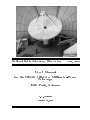
User's Manual
for the NRAO 12 Meter Millimeter-Wave
Telescope
Kitt Peak, Arizona
J. G. Mangum
January 18, 2000
i
Preface
Our intent with this manual is to provide a general reference book for the operation
of the NRAO 12m millimeter-wave telescope. We have included basic material required
for rst-time use of the telescope, as well as more detailed information of possible interest
to all observers. In addition to this manual, we recommend that rst-time users read the
companion document Visitor's Guide to the NRAO 12m Telescope before coming to the
telescope.
We are sure that there is room for improvement in this manual, and ask users to bring to
our attention any errors, omissions, or unclear passages. Please note that we actively
maintain this manual. The most up-to-date version of this document can be
found on the NRAO Tucson Home Page at http://www.tuc.nrao.edu/Tucson.html
and at the telescope.
There are a number of companion documents which you should consult for more detailed
information regarding On-The-Fly observing, the current equipment and calibration status,
and the 1mm Array receiver. The following list itemizes these supplementary documents,
most of which are accessible via the NRAO Tucson Home Page.
The NRAO 12m Telescope Equipment and Calibration Status : Information on current
equipment characteristics, such as receiver temperatures, telescope eÆciencies, etc.
On The Fly Observing at the 12m Telescope : On The Fly data acquisition and analysis
Visitors' Guide to the NRAO 12m Telescope : General guide for prospective observers
Observing with the NRAO 1mm Array Receiver : Observers' guide to the 1mm Array
receiver
Je Mangum
ii
Contents
1 Introduction
1.1 The Observatory . . . . . . . . . . . . . . . . . . . . . . . . . . .
1.2 Observing Proposals . . . . . . . . . . . . . . . . . . . . . . . . .
1.2.1 Proposal Preparation . . . . . . . . . . . . . . . . . . . . .
1.2.2 Proposal Submission and Refereeing . . . . . . . . . . . .
1.2.3 Proposal and Observing Propriety . . . . . . . . . . . . . .
1.3 Observatory Policy . . . . . . . . . . . . . . . . . . . . . . . . . .
1.3.1 Sta Responsibilities . . . . . . . . . . . . . . . . . . . . .
1.3.2 Observer's Responsibilities . . . . . . . . . . . . . . . . . .
1.3.3 Maintenance and Repairs . . . . . . . . . . . . . . . . . . .
1.3.4 Sharing Telescope Facilities with Other Observing Teams .
1.3.5 Observations Under Poor Weather Conditions . . . . . . .
1.3.5.1 High Winds . . . . . . . . . . . . . . . . . . . . .
1.3.5.2 Moisture Accumulation In or On the Dome . . .
1.3.5.3 Sun on the Dish . . . . . . . . . . . . . . . . . .
1.3.5.4 Observations Using Emergency Power Generators
1.3.5.5 Safety Rules . . . . . . . . . . . . . . . . . . . . .
2 Getting Started
2.1
2.2
2.3
2.4
What to Bring to the Telescope . . . .
Startup Checklist . . . . . . . . . . . .
Basic Data Reduction with UniPOPS .
Alternate Data Analysis Packages . . .
2.4.1 CLASS . . . . . . . . . . . . . .
2.4.2 Drawspec . . . . . . . . . . . .
2.5 Data Archiving and Export . . . . . .
3 Instrumentation
.
.
.
.
.
.
.
.
.
.
.
.
.
.
.
.
.
.
.
.
.
.
.
.
.
.
.
.
.
.
.
.
.
.
.
.
.
.
.
.
.
.
.
.
.
.
.
.
.
.
.
.
.
.
.
.
.
.
.
.
.
.
.
.
.
.
.
.
.
.
.
.
.
.
.
.
.
.
.
.
.
.
.
.
.
.
.
.
.
.
.
.
.
.
.
.
.
.
.
.
.
.
.
.
.
.
.
.
.
.
.
.
.
.
.
.
.
.
.
.
.
.
.
.
.
.
.
.
.
.
.
.
.
.
.
.
.
.
.
.
.
.
.
.
.
.
.
.
.
.
.
.
.
.
.
.
.
.
.
.
.
.
.
.
.
.
.
.
.
.
.
.
.
.
.
.
.
.
.
.
.
.
.
.
.
.
.
.
.
.
.
.
.
.
.
.
.
.
.
.
.
.
.
.
.
.
.
.
.
.
.
.
.
.
.
.
.
.
.
.
3.1 Telescope Site Layout . . . . . . . . . . . . . . . . . . . . . . . . . . . . . .
3.2 Telescope Optics . . . . . . . . . . . . . . . . . . . . . . . . . . . . . . . .
3.3 Receivers . . . . . . . . . . . . . . . . . . . . . . . . . . . . . . . . . . . . .
3.3.1 1mm Array Receiver . . . . . . . . . . . . . . . . . . . . . . . . . .
3.3.1.1 1mm Array Rotator and Positioning Conventions . . . . .
3.3.1.2 Pointing and Mapping Osets with the 1mm Array Rotator
3.4 The Local Oscillator System . . . . . . . . . . . . . . . . . . . . . . . . . .
iii
1
1
2
2
3
4
4
4
4
5
5
5
5
6
6
6
6
9
9
10
11
13
13
15
17
19
19
19
20
23
24
25
26
iv
CONTENTS
3.5 The IF Section . . . . . . . . . . . . . .
3.6 Spectrometers . . . . . . . . . . . . . . .
3.6.1 Filter Banks . . . . . . . . . . . .
3.6.2 Millimeter Autocorrelator (MAC)
3.6.3 Continuum Backend . . . . . . .
3.7 Computer Equipment . . . . . . . . . . .
.
.
.
.
.
.
.
.
.
.
.
.
.
.
.
.
.
.
.
.
.
.
.
.
.
.
.
.
.
.
.
.
.
.
.
.
.
.
.
.
.
.
.
.
.
.
.
.
.
.
.
.
.
.
.
.
.
.
.
.
.
.
.
.
.
.
.
.
.
.
.
.
.
.
.
.
.
.
4 Tracking, Pointing, and Focus
4.1 Tracking Capabilities . . . . . . . . . . . . . . . . . . . . . . . .
4.1.1 Ephemeris Objects . . . . . . . . . . . . . . . . . . . . .
4.2 Tracking Limits . . . . . . . . . . . . . . . . . . . . . . . . . . .
4.2.1 Elevation Limits . . . . . . . . . . . . . . . . . . . . . .
4.2.2 Azimuth Limits . . . . . . . . . . . . . . . . . . . . . . .
4.3 Tracking Error Tolerance . . . . . . . . . . . . . . . . . . . . . .
4.4 Sequence of Position Computation Operations . . . . . . . . . .
4.5 Subreector Beam Throw . . . . . . . . . . . . . . . . . . . . .
4.6 Pointing . . . . . . . . . . . . . . . . . . . . . . . . . . . . . . .
4.6.1 Continuum and Spectral Line Five-Point Measurements .
4.6.1.1 Continuum Five-Point Analysis . . . . . . . . .
4.6.1.2 Spectral Line Five-Point Analysis . . . . . . . .
4.6.2 Pointing Model Equations . . . . . . . . . . . . . . . . .
4.6.3 Pointing Data Analysis Program . . . . . . . . . . . . .
4.7 Focus . . . . . . . . . . . . . . . . . . . . . . . . . . . . . . . . .
4.7.1 Axial Focus . . . . . . . . . . . . . . . . . . . . . . . . .
4.7.2 Determining the Axial Focus . . . . . . . . . . . . . . . .
4.7.3 Lateral Focus . . . . . . . . . . . . . . . . . . . . . . . .
5 Spectral Line Observing
5.1 Startup Checklist . . . . . . . . . . . . . . .
5.2 Sideband Choice . . . . . . . . . . . . . . .
5.3 Spectrometers . . . . . . . . . . . . . . . . .
5.3.1 Filter Banks . . . . . . . . . . . . . .
5.3.1.1 The Parallel/Series Option
5.3.1.2 Bad Channel Elimination .
5.3.1.3 Frequency Osets . . . . . .
5.3.2 Millimeter Autocorrelator . . . . . .
5.3.2.1 The 4IF Observing Mode .
5.4 Observing Modes . . . . . . . . . . . . . . .
5.4.1 Total Power ONs and OFFs . . . . .
5.4.2 Position Switching . . . . . . . . . .
5.4.3 Absolute Position Switching . . . . .
5.4.4 Frequency Switching . . . . . . . . .
5.4.5 Beam Switching . . . . . . . . . . . .
5.4.6 Mapping . . . . . . . . . . . . . . . .
5.4.6.1 Manual Osets . . . . . . .
.
.
.
.
.
.
.
.
.
.
.
.
.
.
.
.
.
.
.
.
.
.
.
.
.
.
.
.
.
.
.
.
.
.
.
.
.
.
.
.
.
.
.
.
.
.
.
.
.
.
.
.
.
.
.
.
.
.
.
.
.
.
.
.
.
.
.
.
.
.
.
.
.
.
.
.
.
.
.
.
.
.
.
.
.
.
.
.
.
.
.
.
.
.
.
.
.
.
.
.
.
.
.
.
.
.
.
.
.
.
.
.
.
.
.
.
.
.
.
.
.
.
.
.
.
.
.
.
.
.
.
.
.
.
.
.
.
.
.
.
.
.
.
.
.
.
.
.
.
.
.
.
.
.
.
.
.
.
.
.
.
.
.
.
.
.
.
.
.
.
.
.
.
.
.
.
.
.
.
.
.
.
.
.
.
.
.
.
.
.
.
.
.
.
.
.
.
.
.
.
.
.
.
.
.
.
.
.
.
.
.
.
.
.
.
.
.
.
.
.
.
.
.
.
.
.
.
.
.
.
.
.
.
.
.
.
.
.
.
.
.
.
.
.
.
.
.
.
.
.
.
.
.
.
.
.
.
.
.
.
.
.
.
.
.
.
.
.
.
.
.
.
.
.
.
.
.
.
.
.
.
.
.
.
.
.
.
.
.
.
.
.
.
.
.
.
.
.
.
.
.
.
.
.
.
.
.
.
.
.
.
.
.
.
.
.
.
.
.
.
.
.
.
.
.
.
.
.
.
.
.
.
.
.
.
.
.
.
.
.
.
.
.
.
.
.
.
.
.
.
.
.
.
.
.
.
.
.
.
.
.
.
.
.
.
.
.
.
.
.
.
.
.
.
.
.
.
.
.
.
.
.
.
.
.
.
.
.
.
.
.
.
.
.
.
.
.
.
.
.
.
.
.
.
.
.
.
.
.
.
.
.
.
.
.
.
.
.
.
.
.
.
.
.
.
.
.
.
.
.
.
.
.
27
28
28
28
29
29
31
31
32
33
33
34
34
34
36
38
38
45
45
48
48
48
48
51
51
55
55
56
57
57
57
57
60
60
60
63
63
64
66
66
70
71
71
v
CONTENTS
5.5
5.6
5.7
5.8
5.9
5.4.6.2 Grid Mapping . . . . . . . . . . . . . . . . . .
5.4.6.3 When Should I OTF Instead of Grid Map? .
5.4.6.4 An Important Note About Spatial Sampling .
Spectral Line Sensitivities . . . . . . . . . . . . . . . . . . . .
Calibration . . . . . . . . . . . . . . . . . . . . . . . . . . . .
5.6.1 Vane Calibration . . . . . . . . . . . . . . . . . . . . .
5.6.2 Direct Calibration . . . . . . . . . . . . . . . . . . . .
Signal Processing . . . . . . . . . . . . . . . . . . . . . . . . .
5.7.1 Position and Frequency Switched Data . . . . . . . . .
5.7.1.1 Vane/Chopper Calibrates . . . . . . . . . . .
5.7.1.2 No-Cal Signal Processing . . . . . . . . . . .
5.7.2 Beam Switched Data . . . . . . . . . . . . . . . . . . .
Changing the Intermediate Frequency . . . . . . . . . . . . . .
Spectral Line Status Monitor . . . . . . . . . . . . . . . . . .
6 Continuum Observing
6.1 Startup Checklist . . . . . . . . . . . . . . . . . . . . . . .
6.2 Selecting an Observing Frequency . . . . . . . . . . . . . .
6.3 Observing Basics . . . . . . . . . . . . . . . . . . . . . . .
6.3.1 Switching Modes . . . . . . . . . . . . . . . . . . .
6.3.2 Checking the Subreector Throw . . . . . . . . . .
6.3.3 Continuum Sensitivity . . . . . . . . . . . . . . . .
6.3.4 The Digital Backend . . . . . . . . . . . . . . . . .
6.3.5 Software Signal Processing of Digital Backend Data
6.4 Observing Procedures . . . . . . . . . . . . . . . . . . . . .
6.4.1 Point Source ON/OFF Observing Procedures . . .
6.4.1.1 The ON/OFF Sequence . . . . . . . . . .
6.4.2 Mapping Extended Sources . . . . . . . . . . . . .
6.4.2.1 Grid Mapping . . . . . . . . . . . . . . . .
6.4.2.2 Continuum On-The-Fly Mapping . . . . .
6.5 Utility Observing Routines . . . . . . . . . . . . . . . . . .
6.5.1 Sky Tip Procedures . . . . . . . . . . . . . . . . . .
6.5.1.1 The SPTIP Analysis Procedure . . . . . .
6.5.1.2 The STIP Reduction Procedure . . . . . .
6.6 Calibration . . . . . . . . . . . . . . . . . . . . . . . . . .
6.6.1 Vane Calibration . . . . . . . . . . . . . . . . . . .
6.6.2 Hot/Cold-Load Calibration . . . . . . . . . . . . .
6.6.3 Calibration of the Flux Density Scale . . . . . . . .
6.7 Continuum Status Monitor . . . . . . . . . . . . . . . . . .
A Pointing Equations for the 12m Telescope
.
.
.
.
.
.
.
.
.
.
.
.
.
.
.
.
.
.
.
.
.
.
.
.
.
.
.
.
.
.
.
.
.
.
.
.
.
.
.
.
.
.
.
.
.
.
.
.
.
.
.
.
.
.
.
.
.
.
.
.
.
.
.
.
.
.
.
.
.
.
.
.
.
.
.
.
.
.
.
.
.
.
.
.
.
.
.
.
.
.
.
.
.
.
.
.
.
.
.
.
.
.
.
.
.
.
.
.
.
.
.
.
.
.
.
.
.
.
.
.
.
.
.
.
.
.
.
.
.
.
.
.
.
.
.
.
.
.
.
.
.
.
.
.
.
.
.
.
.
.
.
.
.
.
.
.
.
.
.
.
.
.
.
.
.
.
.
.
.
.
.
.
.
.
.
.
.
.
.
.
.
.
.
.
.
.
.
.
.
.
.
.
.
.
.
.
.
.
.
.
.
.
.
.
.
.
.
.
.
.
.
.
.
.
.
.
.
.
.
.
.
.
.
.
.
.
.
.
.
.
.
.
.
.
.
.
.
.
.
.
.
.
.
.
.
.
.
.
.
.
.
.
.
.
.
.
.
.
.
.
.
.
.
.
.
.
.
.
.
.
.
.
.
.
.
.
.
.
.
.
.
.
.
.
.
.
.
.
.
.
.
.
.
.
.
.
.
.
.
.
.
.
.
.
.
71
74
74
75
77
77
78
79
79
79
80
80
81
82
87
87
88
88
90
90
92
93
94
96
96
96
98
98
99
99
99
100
101
103
103
105
108
109
113
A.1 Primary Pointing Equations . . . . . . . . . . . . . . . . . . . . . . . . . . 113
A.1.1 Secondary Pointing Corrections . . . . . . . . . . . . . . . . . . . . 115
vi
CONTENTS
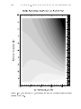
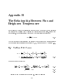
B The Relationship Between Flux and Brightness Temperature
117
C Temperature Scales and Telescope EÆciencies
119
B.1 Uniform Disk Source . . . . . . . . . . . . . . . . . . . . . . . . . . . . . . 117
B.2 Elliptical Gaussian Source . . . . . . . . . . . . . . . . . . . . . . . . . . . 118
C.1 Denitions . . . . . . . . . . . . . . . . .
C.2 Relations Between Temperature Scales .
C.3 Telescope EÆciency Measurements . . .
C.3.1 Corrected Main Beam EÆciency .
C.3.2 Main Beam EÆciency . . . . . .
.
.
.
.
.
.
.
.
.
.
.
.
.
.
.
.
.
.
.
.
.
.
.
.
.
.
.
.
.
.
.
.
.
.
.
.
.
.
.
.
.
.
.
.
.
.
.
.
.
.
.
.
.
.
.
.
.
.
.
.
.
.
.
.
.
.
.
.
.
.
.
.
.
.
.
D Spectral Resolution and Sensitivity Bandwidth in Spectrometers
D.1 Function Integrals .
D.1.1 Sinc . . . .
D.1.2 Gaussian . .
D.1.3 Hanning . .
D.1.4 Hamming .
.
.
.
.
.
.
.
.
.
.
.
.
.
.
.
.
.
.
.
.
.
.
.
.
.
.
.
.
.
.
.
.
.
.
.
.
.
.
.
.
.
.
.
.
.
.
.
.
.
.
.
.
.
.
.
.
.
.
.
.
.
.
.
.
.
.
.
.
.
.
.
.
.
.
.
.
.
.
.
.
.
.
.
.
.
.
.
.
.
.
.
.
.
.
.
.
.
.
.
.
.
.
.
.
.
.
.
.
.
.
.
.
.
.
.
.
.
.
.
.
.
.
.
.
.
.
.
.
.
.
.
.
.
.
.
.
.
.
.
.
.
.
.
.
.
.
.
.
.
.
.
.
.
.
.
.
.
.
.
.
.
.
.
.
.
.
.
.
.
.
.
.
.
.
.
119
121
122
122
122
125
126
126
126
127
127
E Walsh Function Modulation
129
F The Radiometer Equation for Position Switched Measurements
133
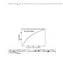
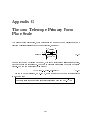
G The 12m Telescope Primary Focus Plate Scale
137
Chapter 1
Introduction
1.1 The Observatory
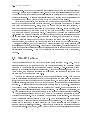
The National Radio Astronomy Observatory (NRAO) 12 Meter Telescope is a general
purpose radio astronomical observatory that supports spectral line and continuum observations in the atmospheric windows at 3 mm, 2 mm, and 1.2 mm wavelengths. The facility
is located on Kitt Peak, Arizona, approximately 50 miles southwest of Tucson. The Observatory was constructed in 1967 with an original surface diameter of 36 feet (11 meters).
In 1982, the surface and backup structure were replaced with a 12m diameter reector.
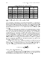
Table 1.1 lists basic information on the observatory site and telescope.
The NRAO operates the telescope as a visitor facility, open to use by competent observers without regard to aÆliation or nationality. Proposals are accepted before three
deadlines each year and are evaluated by a panel of anonymous referees (see x1.2 for
more information on proposal submission). The telescope is open for visitor use from approximately September 15th to July 15th each year. From late July through the middle
of September the prevailing weather pattern precludes observations at millimeter wavelengths and the telescope operation is shut down. Extensive overhauls, telescope upgrades
and major maintenance are done during the summer shutdown period.
The 12 Meter Telescope is one of ve observatory units operated by the NRAO. The
NRAO is administered by Associated Universities, Inc. (AUI), under cooperative agreement with the National Science Foundation. Operations of the 12 Meter Telescope are
managed by the Assistant Director who, with the Assistant Scientists, also handles the
scheduling of the instrument. The Assistant Director or Deputy Assistant Director should
be contacted with regard to general matters of operations policy. In addition, more general
questions or comments pertaining to Observatory-wide activities (scheduling procedures,
scientic or instrumentation priorities, inter-site relations) or specic criticisms of, or suggestions for, the Tucson operation may be addressed to the Director of the NRAO located
at the Charlottesville, Virginia oÆce.
Additional visitor information, including maps, lodging fees, travel reimbursement policies, and names of specic sta members responsible for operation of the telescope can be
found on the NRAO Tucson Home Page at http://www.tuc.nrao.edu/Tucson.html. This
information can also be found in the companion document, Visitors' Guide to the NRAO
1
2
CHAPTER 1. INTRODUCTION
Table 1.1: Telescope and Site Characteristics
Site
Telescope
East Longitude:
North Latitude:
Elevation:
111Æ 360 53.00475
+31Æ 570 12.000
1894.5 meters (6215.8 feet)
Primary Reector Diameter:
Focal Ratio (f/D)
Prime Focus:
Cassegrain Focus:
Surface Accuracy:
Mount:
Slew Rate:
Pointing Accuracy:
Elevation Limit:
Enclosure:
12.0 meters
0.42
13.8
75 m rms
Elevation over Azimuth
68Æ/minute
500 rms
15Æ
Tracking astrodome with movable door
12m Telescope.
1.2 Observing Proposals
1.2.1 Proposal Preparation
All proposals should include a completed 12m Observing Application Cover Sheet. The
body of the proposal must include:
1. A concise scientic justication for the project (Do not exceed 1000 words);
2. An estimate of the observing time required;
3. Frequencies and source coordinates to be observed.
As a proposer, you should insure that the project is within the capabilities of the telescope, both in terms of available equipment and the sensitivities and integration times
required. The telescope and receiver parameters and system sensitivities given in x3.3
will be of use in estimating the required integration times. The most up-to-date information on these parameters can be found in the companion document The NRAO
12m Telescope Equipment and Calibration Status and on the NRAO Tucson Home Page
(http://www.tuc.nrao.edu/Tucson.html).
The 12m management imposes no hard rules as to the maximum or minimum lengths
of observing programs. A typical 12m observing run lasts 3 or 4 days of either partial or
1.2. OBSERVING PROPOSALS
3
Table 1.2: Proposal Submission Deadlines
Deadline
Observing Period
January 1
April to mid-July
July 1 mid-September to December 31
October 1
January 1 to March 31
around-the-clock time. Requests for more than 5 days of time usually receive close scrutiny
by the referees and scheduling committee. If only a specic LST range is required, you
should request only that range.
For any proposal period, the Scheduling Committee always receives more proposals
than can be scheduled; the requested time often exceeds the available time by factors of 2
{ 4. For this reason, you should prepare proposals with care.
1.2.2 Proposal Submission and Refereeing
Twelve meter telescope scheduling operates on a trimester system, with proposal submission deadlines and their corresponding observing periods listed in Table 1.2. The intention
of the 12m proposal system is to insure that the projects granted telescope time are of
current interest and that all proposals receive a prompt scheduling decision.
Proposals should be sent to the Director of the NRAO in Charlottesville, Virginia. Information regarding electronic submission of proposals can be found on the NRAO Tucson
Home Page (http://www.tuc.nrao.edu/Tucson.html). After receipt by the Director's oÆce,
the proposals are assigned a reference number and are sent to a panel of ve referees who
are anonymous to the proposer and to each other. The referees rank the proposal as to
scientic merit and feasibility of achieving the scientic goal, recommend what percentage of the requested observing time should be granted, and make any comments they feel
are pertinent. On the basis of the referees' rankings and comments, the 12m Scheduling
Committee selects the proposals to be scheduled. A report of referees' comments and the
disposition of the proposal is sent to the proposal's contact authors, usually within 6-8
weeks after the deadline.
Proposals are considered for two consecutive trimester periods. On a proposal's second
consideration, it will be in competition with new proposals received for that period. If
a proposal is not selected on its second consideration, it will be declared inactive and
generally will not receive any further consideration for telescope time.
The 12m Scheduling Committee will notify proposers as to the disposition of their active
proposals after each selection process. After any evaluation of a proposal, the authors may
submit an amended version of the proposal to address referees' remarks or to otherwise
strengthen the proposal. The proposal will be re-refereed for the next available period.
Investigators are also free to withdraw a proposal and resubmit it as a dierent proposal.
4
CHAPTER 1. INTRODUCTION
1.2.3 Proposal and Observing Propriety
Observers are expected to conne their observations to those described in their refereed
proposal. It is absolutely essential that observers consult with the Assistant Director
or Deputy Assistant Director and obtain his approval before altering scheduled observing
programs. Approval for changes can be granted under those circumstances that do not lead
to an infringement on work proposed by others, and when the changes are in keeping with
the spirit of the original, refereed proposal. These rules are fundamental to the integrity
of the observing system at NRAO and are taken very seriously by the management.
1.3 Observatory Policy
1.3.1 Sta Responsibilities
The following is the responsibility of the NRAO sta:
To insure that the equipment needed for your observations is available and installed
at the telescope.
To tune the receiver to the desired frequency.
To provide sound telescope pointing.
To provide fundamental telescope calibration parameters { eÆciencies, beamwidths,
gain curves { at standard observing frequencies.
To provide advice on observing strategies, if requested.
1.3.2 Observer's Responsibilities
As the visiting observer, you have the responsibility for proper supervision of all aspects
of the observing program. This includes:
Providing to the NRAO sta, well in advance of the time scheduled, a full description
of the equipment needed for the observations as well as a complete list of frequencies
to be observed. Usually this information is included on the proposal cover sheet.
To verify the telescope pointing and ne-tune it as needed.
To obtain all calibration and other receiver/telescope parameters necessary for data
reduction. This can be done either by adopting or scaling the NRAO-provided information from standard frequencies, and/or by making the appropriate measurements.
In either case, proper data calibration is your responsibility, not the NRAO's.
To inform the NRAO sta, before the observing period has ended, about the types
of data to be written on an export tape, and the format of the export tape.
In addition, you are requested to provide feedback on the observing run via the \Observer's
Comment Sheet", available at the telescope and on the NRAO Tucson Home Page.
1.3. OBSERVATORY POLICY
5
1.3.3 Maintenance and Repairs
One period approximately every 10 days is assigned to preventive maintenance and routine
system tests. If during a scheduled observing period a catastrophic failure of the instrument
occurs which results in a loss of data, observations will be stopped and the NRAO technical
sta will attempt to repair the equipment. In less serious cases where data-taking continues
but where the quality of the data is not optimal, it is your responsibility to decide whether
or not you wish to give up telescope time so that repairs can be made. Only the Tucson
Assistant Director can make the decision to interrupt scheduled operations to make nonessential repairs.
1.3.4 Sharing Telescope Facilities with Other Observing Teams
Since living quarters and work spaces at the telescope are limited, you should leave the
mountain as soon as possible at the end of your run, allowing, of course, for a reasonable
period of rest. If you wish to continue the reduction of your data sets, you should do so at
the NRAO Tucson oÆce. When two or more observing teams are sharing observing time,
the team currently observing has priority to all telescope facilities, including computer
usage. The other observing teams should endeavor to stay out of the control room and
not interfere in any way with the ongoing observations. Unless one group of observers is
declared the \prime observer" on the telescope schedule, equipment changes needed for a
program will be done at the beginning of that program's time.
1.3.5 Observations Under Poor Weather Conditions
There are a variety of weather conditions which can endanger the safety of the telescope.
It is the responsibility of the telescope operator to take appropriate action if any of the
conditions listed below occur.
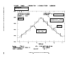
1.3.5.1 High Winds
If the wind exceeds 15 mph, observations will be restricted to those quadrants where
the telescope drive motor currents are not excessive.
If the steady wind, or the average of gusty wind, exceeds 35 mph the dome door
must be closed. Observations can be continued through the side of the dome.
For winds above 45 mph, the dome door must be positioned 180Æ from the direction
of the wind and held xed. Observations can continue through the side of the dome,
but the dome cannot be moved.
If the wind exceeds 55 mph operations must cease and the telescope must be placed
in the service position with the stow pins in place.
6
CHAPTER 1. INTRODUCTION
1.3.5.2 Moisture Accumulation In or On the Dome
If there is fog in the dome, or if moisture is condensing on the antenna or equipment, the
dome door will be closed. Observations can continue through the side of the dome. If
there is a build-up of snow/ice on the dome, the accumulated snow/ice must be cleared
from the dome door before observations can resume.
1.3.5.3 Sun on the Dish
The pointing and focus of the dish can be seriously aected if the sun is allowed to shine
on the surface of the dish or the feed support legs. If accurate pointing is desired, care
must be taken to keep the sun o the dish. To avoid excessive heating of the feed legs,
the prime focus regions, and the cables to the prime focus, the dish will not be pointed to
within 15 degrees of the sun. The projected distance between the sun and a position on
the sky dened as (AZobj ,ELobj ) is given by the following equation:
cos(Dobj ) = cos(90
EL ) cos(90 ELobj )+sin(90 EL ) sin(90 ELobj ) cos(AZobj AZ )
(1.1)
1.3.5.4 Observations Using Emergency Power Generators
The telescope and dome have three sources of electric power { the commercial source and
two power generators. Observations can continue as long as at least two of the sources are
operational. If only one source of power is available, the dome door must be closed.
1.3.5.5 Safety Rules
The following safety rules obtain at the 12 Meter Telescope site. We expect all observers
and visitors to the site to read and abide by these rules.
1. To drive a GSA car, you must possess a valid driver's license.
2. The Telescope Operator on duty is the only person allowed to operate the telescope.
3. Observers are not to be on the telescope unless the duty operator has specically
authorized them to be there.
4. Safety chains and rails have been installed at the entrance to the observing rooms.
They are there to prevent you from walking into any possible pinch points or dangerous areas.
5. Do not stand in the red areas because parts of the telescope and dome that move in
those areas could injure you severely.
6. Do not touch the yellow curtains around the inside wall of the dome. Behind them
are exposed 480-volt power lines.
1.3. OBSERVATORY POLICY
7
7. Please abide by all printed and posted safety rules such as \No Smoking" and \Do
Not Enter This Area" posters, etc.
8. Only the telescope operator or other qualied Arizona employees are allowed to
operate the \cherry picker". Observers may ride in the cherry picker if authorized to
do so by the duty operator.
9. Hard hats are required for all persons in the dome area if someone is working above
or in the cherry picker. The hats are located on the wall just outside of the observing
room door.
10. When walking outside to the dormitories or the lab at night, please be sure to carry
a ashlight. You may encounter steps, drop-os, or hungry wild animals.
11. The consumption of alcoholic beverages or illegal drugs is absolutely forbidden in the
lab and telescope/control room areas.
12. All employees and observers are required to wear seat belts while riding in government
vehicles.
13. Ice, rocks, and rock slides are frequently a hazard on the roads and walkways. Cattle
and horses cross Highway 386 and several have been hit. Please drive and walk
carefully.
14. Please drive very slowly and carefully in all NOAO and NRAO parking or road areas.
Pedestrians, including small children seem to leap out at cars on a regular basis.
15. A more complete list of safety rules and recommendations is available in the observers'
lounge and from the telescope operator. You might nd it interesting reading, although not required.
8
CHAPTER 1. INTRODUCTION
Chapter 2
Getting Started
2.1 What to Bring to the Telescope
Your observations will be more eÆcient and you will achieve better results if you have
thoroughly prepared for your observing run before arriving at the telescope. Most of this
work should be done at the time the proposal is written (see Chapter 1). For both spectral
line and continuum observations, you should prepare the following before coming to the
telescope:
Source List: A source list with epoch B1950 or J2000 RA and Dec or (lII, bII) Galactic
coordinates. For spectral line observations you will also need the source velocities
in the LSR, optical, or relativistic velocity reference frames (see Chapter 4). Keep
in mind that the beam sizes for the 12m can be quite small (2000) at the higher
frequencies so the positions should be appropriately accurate. You can save time by
composing your catalog prior to your observing run. See Chapter 4 for the source
catalog format.
Line Rest Frequencies: You should have line rest frequencies which are accurate to
at least 10 kHz. If emission lines are weak, test line frequencies should be included.
For continuum measurements, choose your observing frequencies so that no strong
spectral lines lie in either of the receiver sidebands.
Observing Mode: The available observing modes for spectral line observations are
Total Power Measurements
Relative and Absolute Position Switching
Frequency Switching
Beam Switching
Grid Mapping
On-The-Fly Mapping
while the available observing modes for continuum observations are
9
10
CHAPTER 2. GETTING STARTED
Switched or Total Power ON/OFF's
Grid Mapping
On-The-Fly Mapping
Reference Positions: The reference oset position, in angle or frequency, should also be
considered carefully. If you are using beam switching, you should consider carefully
the optimum beam separation. The default beam throws are 20 at 3 and 2mm
wavelengths, and 10 at 1mm wavelengths.
Spectrometer Conguration: For spectral line observations you need to determine
how you will congure the lter banks and Millimeter Autocorrelator (MAC), including the resolution and the mode of operation. This decision hinges on the resolution and total bandwidth required. No rm rules exist, but the minimum resolution
acceptable should probably give 3 { 5 channels across the line and the minimum
bandwidth should have 10 { 20% of the band on each side of the line.
2.2 Startup Checklist
A general startup checklist for both spectral line and continuum observations is given below.
Although the Observatory sta tries to provide a fully functional system and advice about
calibration constants and procedures, the responsibility for the integrity of the data rests
with the observer. This checklist will help insure that the system is congured properly
and that variable quantities such as pointing and focus are properly set. Completion of
this checklist may take an hour or more, but the time will be well-spent.
1. Have the operator tune the receiver to the desired frequency, including sideband and
harmonic checks.
2. Select a strong continuum source from the list of standard sources (see Chapter 4).
A bright planet (i.e., Venus, Mars, Saturn, or Jupiter) is preferable. Pick one whose
position is near the rst program source, if possible.
3. Ask the operator to perform a ve-point map of the source to check for pointing
osets. Records of recent pointing osets are kept on graphs near the observer's
console and can be used to estimate an initial value for the1 pointing. The operator will
need to know the map grid spacing (the default value is 2 the beam FWHM) and the
integration time per point. A detailed discussion of telescope pointing characteristics
is given in Chapter 4. When the ve-point measurement is complete, a t will be
made to the measurement on-line and displayed on the on-line data server. You can
also reduce these measurements by hand using UniPOPS (see x2.3). If the t to the
ve-point is poor, repeat the measurement with updated pointing.
4. Ask the operator to perform a focalize on the chosen continuum source. This checks
for the best value of the axial focus. The focalize measurement requires that you
specify a rst guess for the focus position (called F0) and the spacing between the
2.3. BASIC DATA REDUCTION WITH UNIPOPS
11
focus settings (called WL). The system will automatically set F0 to a reasonable
starting value (usually around 45 mm). WL is usually chosen to be 21 the observing
wavelength. When the focalize measurement is complete, a t will be made to the
measurement on-line and displayed on the on-line dataserver. You can also reduce
these measurements with the condar analysis program. See Chapter 4 for more focus
information and x2.3 for data reduction commands. If the t to the focalize is poor,
repeat the observation with an updated value for F0.
NOTE: Pointing and focus may change as the temperature of the dish (or parts of
the dish) changes. Pointing and focus should be checked (at least) after nightfall and
daybreak and more frequently if the dish is illuminated by the sun.
5. For spectral line observations, you should perform the following checks to insure
that the receiver is tuned correctly, the spectrometer is properly congured, and the
calibration scale is correct.
(a) If the program line is weak and no other strong lines are in the bandpass, tune
rst to a strong test line that is as close by in frequency as possible. \Strong"
means any line that will produce a good signal-to-noise spectrum in a 5 { 10
minute integration, for example. Standard sources are listed in the NRAO
standard catalog (called \standard.cat"). If possible, use the same observing
setup (same spectrometer mode and observing mode) as will be used for the
program observations. If the observations are of a common species, such as CO,
there is no need to tune to another line.
(b) Perform a calibration scan and check for bad channels in the lter banks. Report
the bad channels to the operator, who will ag those channels in the control
system software.
(c) Observe a test line in a strong source. Observers may wish to verify the sense
of the velocity/frequency scale by shifting the rest frequency or center velocity
by a small amount and seeing if the line moves in the correct direction for the
sideband choice.
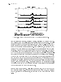
(d) Check that the line temperature calibration is correct. This can be done by
observing a standard source, presuming that the test line has known strength.
Measurements of many of the sources in the NRAO standard catalog \standard.cat" have been made in the CO, 13CO, and C18 O J = 1 ! 0 and J = 2 ! 1
transitions. Plots of these spectra can be found at the telescope and on the
NRAO Tucson Home Page.
2.3 Basic Data Reduction with UniPOPS
Two other manuals, one for spectral line and one for continuum, describe the data reduction
systems in use at the 12m. These are available at the telescope and upon request. The
discussion below is intended only as a quick reference list to help the observer get started.
Raw data is accumulated into two data les; one which contains lter bank data and a
second which contains Millimeter Autocorrelator (MAC) data. Both of these les are in the
12
CHAPTER 2. GETTING STARTED
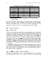
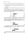
Table 2.1: Subscan Codes For 12m Data
Subscan
Conguration
Filter Banks
01
IF1 in lter bank 1 (series) or rst half of lter bank 1
(parallel)
02
IF1 in second half of lter bank 1 (parallel)
03
IF2 in lter bank 2 (series) or rst half of lter bank 2
(parallel)
04
IF2 in second half of lter bank 2 (parallel)
Millimeter Autocorrelator
11, 12, ..., 18 IF1, IF2, ..., IF8 for 1mm Array observations
11
IF1 in 2IF mode or IF1 at frequency 1 in 4IF mode
12
IF2 in 2IF mode or IF1 at frequency 2 in 4IF mode
13
IF2 at frequency 1 in 4IF mode
14
IF2 at frequency 2 in 4IF mode
Single-Beam Continuum
01
IF1
02
IF2
1mm Array Continuum
01, 02, ..., 08 IF1, IF2, ..., IF8
\sdd" or Single Dish Data format. Each of these les has an associated gains, or \gsdd",
le which contains results for spectral line calibration scans. In the following we give a
brief introduction to the analysis of the spectral line and continuum data accumulated into
these data les.
Before observations begin, the operator will set up a subdirectory containing data les.
This subdirectory is private to each observing team, and is denoted by /obs/ini, where
ini are the 3 letter initials of the lead observer. The data les in this subdirectory are
also labeled with the same initials. Log into the system as username obs (the operator
can tell you the current password for this account). You will then be prompted for your
initials, discussed above. After the login process is complete, you will be in your /obs/ini
subdirectory.
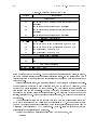
The spectral line system always records data from two 256 channel lter banks and
up to 65536 channels from the Millimeter Autocorrelator (MAC). Each scan is composed
of a number of subscans/indexdata!subscan which individually contain one lter bank or
Millimeter Autocorrelator (MAC) measurement. Table 2.1 lists the subscan codes with
their associated polarizations and backends.
To start the continuum analysis program from the Unix prompt, type
condar
2.4. ALTERNATE DATA ANALYSIS PACKAGES
13
while to start the spectral line analysis program at the Unix prompt, type
line
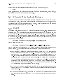
Table 2.2 lists a number of condar and line commands and their function, while Table 2.3
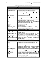
lists a number of basic data analysis procedures.
2.4 Alternate Data Analysis Packages
There are a number of other data analysis packages available at the 12m which can be used
to analyze 12m data. All of these packages require a conversion of the 12m sdd-format to
the resident format of the analysis package to be used. Below I describe the most popular
alternate analysis packages in use at the 12m.
2.4.1 CLASS
Conversion of sdd-format data to CLASS format is currently done on-line. All scans except
continuum and OTF measurements are automatically converted to CLASS format and put
in a le called class.12m in the observer's directory. One can also convert other sdd-format
data les to CLASS format using a utility program called uni2class. To convert all data
in the sdd le sdd.jgm 001, issue the following command from any Unix prompt on any of
the mountain workstations:
uni2class /home/data/jgm/sdd.jgm 001 sdd.jgm 001.class
for the lter bank data and
uni2class /home/data/jgm/sdd hc.jgm 001 sdd hc.jgm 001.class
for the Millimeter Autocorrelator (MAC) data. The second parameter in uni2class is the
output le name. The current features and limitations of this conversion are:
Each spectrum is assigned a unique observation number in the CLASS le according
to the perscription described in Table 2.4. For lter bank data, the nomenclature
used for the CLASS telescope eld identier is \FB" for lterbank followed by a
two-number identier indicating which lter bank (there can be only two) and which
polarization from a lter bank this scan represents. For Millimeter Autocorrelator
(MAC) data, the nomenclature used is \MAC" followed by a two-number identier
indicating which rest frequency (there can be two) and which polarization from a
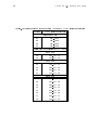
given frequency this scan represents. CLASS does not support subscan numbers.
The original scan number is preserved in the header.
The UniPOPS backend descriptor is converted to a more useful identier which is
inserted into the CLASS telescope eld to avoid ambiguities between subscans for a
particular scan.
Map osets are carried over. There seem to be small (<100) discrepancies in times
and coordinates between the sdd and CLASS les which are perhaps due to roundo
error.
14
CHAPTER 2. GETTING STARTED
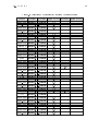
Table 2.2: Analysis Commands in UniPOPS
Command
Function
Commands Common to Both condar and line
get scan number.nn
Retrieves scan number.nn into the work area.
xx
Alias for \page show", which plots scan number.nn following a \get".
header
Displays the header from scan number following a \get".
scan number add
Adds scan number to the stack.
beg scan end scan add Adds all of the scans between beg scan and end scan to
the stack.
c#
Averages all of the scans in the stack and displays the
average for channel # (where # is 1 or 2).
cb
Averages all of the scans in the stack and displays the
average for channels 1 and 2 combined.
tell stack
Lists scans in the stack.
empty
Empties the stack.
yrange(ymin,ymax)
Sets the vertical scale to the range ymin to ymax.
freey
Resets automatic scaling for the y-axis.
Commands Specic to condar
scan number.nn s
Gets and displays the continuum ON/OFF sequence
scan number.nn.
scan number.nn s ave Gets, displays, and prints the average and rms ux of
the continuum ON/OFF sequence scan number.xx
scan number.nn f
Analyzes and plots a ve-point map of scan number.nn
scan number.nn focalize Analyzes and plots a axial focus measurement of
scan number.nn.
scan number.nn sptip Analyzes and plots a sky tip measurement.
Commands Specic to line
fbdata
Tells line that you wish to analyze lter bank data.
hcdata
Tells line that you wish to analyze Millimeter Autocorrelator (MAC) data.
g#
Displays the most recent chopper wheel calibration array
for lter bank number # (where # is either 1 or 2).
gget# scan number
Gets and displays the calibration scan associated with
lter bank # of scan number (where # is either 1 or 2).
scan number f
Gets and displays the rst lter bank of scan number.
scan number s
Gets and displays the second lter bank of scan number.
halves
Displays the average of two lter bank polarizations acquired in \parallel mode".
gcopy
Make a laser printer plot of the graphics screen.
2.4. ALTERNATE DATA ANALYSIS PACKAGES
15
Table 2.3: Analysis Procedures in line
Command
Function
badch
Starts interactive bad channel agging procedure.
bset
Interactive procedure to set baseline t parameters.
nt = n
Sets the baseline order to n.
baseline xx
Fits, subtracts, and plots the resulting baseline.
gset
Interactive procedure to set gaussian t parameters.
gauss
Fits gaussians.
gparts
Plots individual gaussian ts (for multiple gaussians)
and lists height, FWHP width, and position for each
gaussian.
gdisplay
Plots sum of gaussian ts and lists characteristics.
center scan number vel# Processes the spectra for a total power spectral line vepoint measurement from lter bank #, where # is either
1 or 2.
CLASS and uni2class can access the data le at the same time. This means that you
can read the CLASS le at the same time as you are writing to it.
uni2class will overwrite existing output les without warning. Be careful!
Only LSR and heliocentric velocities, equatorial coordinates, and the standard small-
eld projection are handled correctly.
No distinction is made between radio and optical velocity denitions.
Continuum data are not handled.
The sdd and CLASS headers do not map onto each other exactly, but nearly all of
the important parameters are mapped.
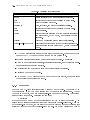
2.4.2 Drawspec
Drawspec is a PC-based analysis program written by Harvey Liszt. The public PC in
the control room at the 12m has a current copy of Drawspec for observer use. To port
your data to Drawspec, you must write a single-dish FITS le of your data. The program
uni2ts will do this for you. Just issue the command
% uni2fits
at the unix prompt on any of the workstations at the 12m to start the program. You
will be asked a series of questions by uni2ts which should be self-explanatory. Once you
have a single-dish FITS le, you can start the Drawspec program and use the "scanmstr"
utility in Drawspec to import the single-dish FITS le. See Harvey Liszt's home page at
16
CHAPTER 2. GETTING STARTED
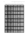
Table 2.4: Correspondence Between Subscan Codes and CLASS Telescope Identiers
Subscan CLASS Telescope Identier
Filter Bank Data
01
12M-FB11
02
12M-FB12
03
12M-FB21
04
12M-FB22
Millimeter Autocorrelator (MAC) Data
2 IF Mode
11
12M-MAC11
12
12M-MAC12
4 IF Mode
11
12M-MAC11
12
12M-MAC21
13
12M-MAC12
14
12M-MAC22
8 IF Mode
11
12M-MAC11
12
12M-MAC12
13
12M-MAC13
14
12M-MAC14
15
12M-MAC15
16
12M-MAC16
17
12M-MAC17
18
12M-MAC18
2.5. DATA ARCHIVING AND EXPORT
17
http://www.cv.nrao.edu/ hliszt/programs.html for more information on Drawspec and its
aÆliated programs.
2.5 Data Archiving and Export
When you have nished your observations, an archive tape of the observers' les will be
made and sent to the Tucson oÆce. If you submit a Data Tape Request Form, the sta
will create an export tape of your data and mail it to your home institution. We oer two
types of export tapes: an ASCII tape following the FITS standard or a tar-format copy of
your sdd les.
18
CHAPTER 2. GETTING STARTED
Chapter 3
Instrumentation
3.1 Telescope Site Layout
The 12m is located on the southwest ridge of Kitt Peak, about two miles below the top of
the mountain. Other telescopes on the southwest ridge are the NRAO 25m VLBA antenna
and the McGraw-Hill Observatory 1.2m and 2.4m optical telescopes. A drawing of the 12m
site layout is given in the Visitor's Guide to the NRAO 12m Telescope and can be found
on the NRAO Tucson Home Page (http://www.tuc.nrao.edu/Tucson.html).
Three rooms are available in the dome for observer use. During scheduled observing
time, you will normally want to sit in the control room at the observer's console so that
you can communicate with the operator. An adjacent \breezeway" room has an additional
workstation and work area. A third room, called the \observer lounge", is available for
work, data reduction, and private phone calls. This room has a couch that can be used
for naps. If two observing teams are sharing time on the telescope, the data reduction
station in the observer lounge is reserved for the team not currently observing. The team
not currently observing should stay out of the control room if at all possible. If more than
two observing teams are sharing time at the telescope, they should negotiate the use of
the observer lounge.
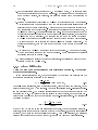
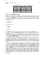
3.2 Telescope Optics
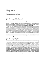
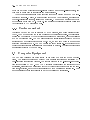
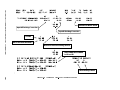
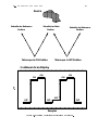
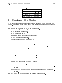
The 12m employs \bent Cassegrain" optics for all of the receivers used by visiting observers.
A few test and special purpose receivers including the holography receiver are mounted at
the prime focus. A diagram of the optics is given in Figure 3.1. The primary mirror is a
12.0 meter paraboloid of 72 aluminum panels. The position of each panel can be adjusted
by stand-o bolts. The subreector (secondary mirror) is mounted at the prime focus and
is supported by a quadrapod feed leg structure. The subreector mounting box contains
the nutation (beam switching) electronics and the solenoid drivers for the switching. The
box also contains a gas discharge noise source and associated electronics. The feed horn of
the noise source protrudes from a hole in the center of the machined-aluminum hyperboloid
subreector. Under normal operation, the noise tube is covered with a cone reector (called
the \Cone of Silence") to minimize standing waves in the IF passband. If you would like
19
20
CHAPTER 3. INSTRUMENTATION
to use the noise tube for calibration, you must let the operator know so that
he can remove the cone reector.
The subreector box is located in a focus-translation mount with three degrees of
freedom of movement. The subreector can be moved in and out along the radio axis
to adjust for axial focus changes, it can be moved in an \up-down" (or \north-south")
direction to compensate for north-south focus changes, or east-west to adjust for optimum
azimuth position.
The tertiary or central mirror is a rectangular at mirror with azimuth and elevation
position adjustments. The elevation position of the mirror is periodically measured and
then clamped down. The azimuth position can be rotated to direct the radio beam to any
of the four receiver bays, located behind the main reector. The central mirror positioning
is motorized and under servo control from the control room, making it possible to use more
than one receiver during a single observing run, though not simultaneously.
The central mirror directs the beam to one of the four quaternary mirrors over each
receiver box. The quaternary mirrors are oval ats and have one degree of freedom for
position adjustment. The optics following the quaternary mirrors are contained within the
receiver boxes and are usually dierent for each receiver.
The alignment of the mirrors is done optically. Small optical mirrors are xed to the
tertiary and quaternary mirrors. A laser is mounted in the subreector position and the
mirrors are adjusted so that the laser beam spot is centered on the receiver lens. The beam
also may be autocollimated at the subreector to achieve the most precise alignment.
3.3 Receivers
All of the receivers in use at the 12m employ heterodyne mixers (sometimes called \coherent detectors") which use superconducting-insulating-superconducting (SIS) junctions.
The SIS junctions are housed in a dewar which is part of a closed-cycle cryostat with temperature stages at 20 K and 4 K. The 20 K stage is cooled by a conventional compressed
helium refrigerator system; the 4 K stage is cooled by a separate Joule-Thomson unit. The
two receivers are mounted in upright structures, variously known as \rockets" or \inserts".
The inserts are wholly self-contained receiver units, and may be removed independently,
albeit by warming the mother dewar. A local oscillator (LO) signal, provided by a Gunn
oscillator, is injected into the mixer or diplexed with the incoming radio frequency (RF)
signal. The output of the mixer is an intermediate frequency that is the dierence between
the LO and RF signal frequencies. The SIS junctions in the 3 and 2mm receivers have
tunable backshorts, which can be adjusted to resonantly cancel the unwanted sideband,
and are essentially single sideband (SSB) mixers. A harmonic generator is switched into
the optical path of the receiver to allow precise measurement of the sideband rejection in
the 2 and 3mm receivers. The image sideband of the 1mm receiver is rejected by inserting
a Martin-Pupplet lter into the LO path. At most frequencies the image sideband can be
rejected to 20 dB.
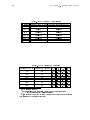
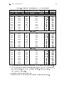
Table 3.1 lists the current tuning ranges and typical system temperatures for all of the
facility 12m receivers, while Table 3.2 lists representive telescope eÆciencies.
21
3.3. RECEIVERS
Nutating Subreflector
Primary Reflector
Quaternary Mirror (1 of 4)
Quaternary Mirror
Central Selection Mirror
(Rotatable to allow access to
any one of four receiver bays)
RX1
RX2
Primary Focal Length = 5.08m
f/D of Final Beam = 13.8
Figure 3.1: 12m Telescope Optics
22
CHAPTER 3. INSTRUMENTATION
Receiver
3mmlo
3mmhi
2mm
1mmlo
1mmhi
1mm8ch
Table 3.1: 12m Receiver Characteristics
Tuning Range (GHz) Approximate Tsys(SSB) (K)
68{90
170{225
90{116
160{350
130{170
180{400
200{265
400{900
260{300
800{1200
215{245
700
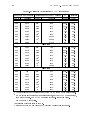
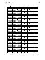
Table 3.2: 12m Telescope EÆciencies
Frequency (GHz) Beamwidth (arcsec) Aa l b
70
90
0.52 0.94
90
70
0.51 0.94
115
55
0.48 0.94
145
43
0.45 0.94
230
27
0.32 0.94
300
21
0.22 0.94
f ss c m d
0.68
0.68
0.68
0.68
0.68
0.68
0.98
0.95
0.85
0.80
0.50
0.30
= aperture eÆciency
= rear spillover and scattering, blockage, and ohmic loss eÆciency
= forward scattering and spillover eÆciency
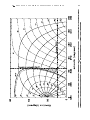
m = corrected main beam eÆciency (percent of power in the main diraction
beam relative to the outlying error beam)
a
A
b
l
c
fss
d 23
3.3. RECEIVERS
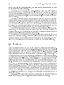
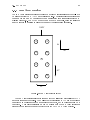
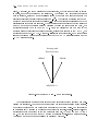
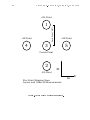
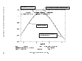
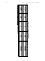
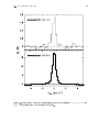
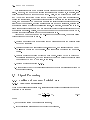
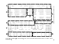
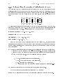
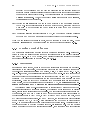
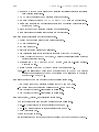
3.3.1 1mm Array Receiver
The 1mm Array receiver is designed for rapid mapping of spectral lines in the 215 { 240
GHz range (notably J = 2 ! 1 CO and its isotopomers). The receiver places 8 independent
beams on the sky in a 2 4 array; each beam is separated from its nearest neighbor by
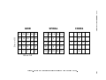
8700 (see Figure 3.2). The FWHM of each beam at 230 GHz is 3000, hence the telescope
must be stepped in position to ll in the beams if Nyquist sampling is desired.
180°
5
4
EL
AZ
3
6
C
2
7
87″
8
1
87″
Figure 3.2: 1mm Array receiver layout
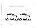
The 1mm Array receiver is intended for use with the Millimeter Autocorrelator (MAC)
and eight channel IF processor. The Millimeter Autocorrelator (MAC) and IF processor
can accept 8 IF channels of 600 MHz or narrower bandwidth, or 4 IF channels of 600 MHz
bandwidth. A complete description on how to observe with the 1mm Array receiver is
given in the companion document Observing with the NRAO 1mm Array Receiver.
24
CHAPTER 3. INSTRUMENTATION
3.3.1.1 1mm Array Rotator and Positioning Conventions
The entire 1mm Array receiver cryostat and optics assembly is housed in a precision
rotation mechanism which can rotate the orientation of the array of beams to an arbitrary
angle on the sky. Thus, the array may be positioned to take advantage of a particular
source geometry. Furthermore, the 1mm Array rotator can then track parallactic angle
so that as the source moves across the sky in hour angle, the orientation of the array is
the same in the RA-DEC frame (because the 12m is an AZ-EL telescope, parallactic angle
rotation must be taken into account). The rotation center of the array is dened to be its
geometric center, i.e., the center of the box dened by beams 2, 3, 6, and 7 (see Figure
3.2).
Three dierent angles come into play in describing the positioning and movement of
the rotator:
The parallactic angle is dened as the angle between lines
of constant azimuth and hour angle. Thus, it is a function of the azimuth, elevation,
hour angle, and declination of the source. The convention employed at the 12m is as
follows:
Source Parallactic Angle:
When a source is on the Prime Meridian (0 Hour Angle) in the south, parallactic
angle is dened to be 0Æ . While the source is above the horizon in the south, parallactic
angle always increases with time. When the source is on the Prime Meridian (upper
culmination) in the north, parallactic angle is dened to be 180Æ . In the north,
parallactic angle decreases with time.
The angle describing the rotation of the 1mm Array rotator
relative to its position encoders. This angle is displayed on the Status monitor. The
convention is stated as follows:
Rotator Control Angle:
When the telescope is pointing due south (180Æ azimuth) and the long dimension of the
array is aligned along the Prime Meridian (up and down in the elevation direction),
with beams 4 and 5 at high elevation (and high declination), the array has a rotator
control angle of 0Æ . If the rotator is turned so that beams 4 and 5 move toward larger
azimuth, the rotator control angle increases.
The user-dened position angle is available to allow the user to
position the rectangular array of beams in the RA/DEC frame to achieve optimal
mapping eÆciency according to the geometry of the source. The most common
example of this would be to position the long dimension of the array of beams along
the major axis of a galaxy. The convention for dening User Position Angle is as
follows:
User Position Angle:
The user-dened position angle follows the usual astronomical position angle convention. Position angle increases toward the east (increasing Right Ascension). Note
that this convention is independent of whether the source is north or south of the
zenith.
3.3. RECEIVERS
25
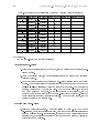
Table 3.3: 1mm Array Azimuth and Elevation Osets Relative to Array Center
Beam Number Azimuth Oset (00) Elevation Oset (00 )
1
43.5
130.5
2
43.5
43.5
3
43.5
43.5
4
43.5
130.5
5
43.5
130.5
6
43.5
43.5
7
43.5
43.5
8
43.5
130.5
3.3.1.2 Pointing and Mapping Osets with the 1mm Array Rotator
The rotation and tracking center of the array is at its geometric center, where no beam
exists. We take account of this fact in pointing and focus measurements by allowing the
user to specify a beam to point or focus on and then calculating the pointing center of the
array based on this measurement.
When the array is rotated from its \null" control angle of 0Æ, the position of the beams
are given by the equations for a Cartesian coordinate system rotation. In the (AZ,EL)
frame the position of an individual beam is given by
Ai = A0 [Ai cos( 0) + Ei sin( 0 )]
Ei = E0 [Ei cos( 0 ) Ai sin( 0 )]
(3.1)
where A0 and E0 are the azimuth and elevation pointing correction for the center of the
array, 0 is the hardware control angle of the array in its null position (0Æ), is the rotator
control angle, and Ai and Ei are the azimuth and elevation osets of the individual beams
relative to the geometric center, and are given by Table 3.3
If you are not tracking parallactic angle (e.g. for a pointing check), then you will be
observing in an (AZ,EL) frame and all positioning osets should be in AZ and EL. If you
are tracking parallactic angle, you will be observing in an (RA,DEC) or (lII,bII) frame and
mapping and beam osets should be given in RA and DEC.
Relations similar to Equations 3.1 exist for (RA,DEC) (or (lII,bII)) osets when the
array is rotated by a user position angle. The equations describing these osets are
RAi = RAi cos() + DECi sin()
(3.2)
DECi = DECi cos() + RAi sin()
(3.3)
where is the position angle and RAi and DECi are the RA and DEC osets of each
beam relative to the rotation center, when the array is at 0Æ position angle. These osets
26
CHAPTER 3. INSTRUMENTATION
are the same as in Table 3.3, with RA corresponding to the Azimuth column and DEC to
the Elevation column. If you wish to convert arc seconds on the sky to seconds of time in
RA, remember to divide by 15 cos(DEC).
3.4 The Local Oscillator System
Mixer receivers require a local oscillator signal. For spectral line work, the LO signal must
be phase and frequency stable to an accuracy of at least 1 part in 105. The purpose of the
LO system is to phase lock the LO source, which is otherwise a free-running oscillator. LO
sources used at the 12m are solid state Gunn oscillators. The power required of the LO
source by present generation millimeter-wave mixers precludes the direct use of a harmonic
of a low frequency synthesizer. At the 12m, a precise synthesizer harmonic is used as a
comparison frequency for the phase lock loop.
A 5 MHz rubidium oscillator is multiplied by 20 to give a frequency of 100 MHz. This
100 MHz drives a comb generator, thus enabling any multiple of the 100 MHz in the range
1-2 GHz to be selected by a lter. Either the 18th or the 19th (1.8 or 1.9 GHz) is usually
selected; a frequency between 50 and 150 MHz is then added and an oscillator is phase
locked to the result. In this way a spectrally pure signal in the range 1.85 to 2.05 GHz is
generated.
This nominal 2 GHz signal is then fed up to the receiver and used to drive a harmonic
mixer. The nth harmonic of the 2 GHz signal (n may be any integer from ten to seventy,
or higher) then mixes with a portion of the receiver LO frequency to produce the lock IF
frequency. For the Gunn oscillator systems, F2 = 100 MHz. The phase lock of the Gunn is
completed by phase detecting this beat frequency with a synthesized loop oset frequency
as a reference. The loop oset frequency is generated by a tunable Fluke synthesizer.
The phase loop will lock when the LO frequency diers from the nth harmonic of the 2
GHz source by the loop oset frequency. This means, of course, two lock points, one with
the LO above the nth harmonic and the other with the LO below. These two points will
be separated by twice the loop oset frequency (200 MHz). The computer tests the loop
for lock while taking data and stops taking data if the loop is found to be unlocked.
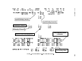
The synthesizer frequency is computed from the following equation:
(fsky +jfIF ) + kf
lock
m
f =
(3.4)
syn
N
where fsyn is the synthesizer frequency, fsky is the sky frequency of the emission (the rest
frequency with Doppler corrections), j = +1 for lower sideband and 1 for upper sideband,
fIF is the IF frequency/indexfrequency!IF, m is the factor by which the LO frequency is
multiplied before injection into the mixer, k = 1 for the lower lock sideband and +1 for
the upper lock sideband, flock is the the phase lock loop oset frequency, and N is the
synthesizer harmonic. The four permutations of j and k are given by a parameter \SB"
(for \sideband") that is entered into the control computer.
The control computer calculates two synthesizer settings (corresponding to dierent
harmonic numbers N) for a given rest frequency, source Doppler velocity, and SB value.
The operator can switch between these two settings by turning a knob on the synthesizer
3.5. THE IF SECTION
27
control chassis. The computer chooses the synthesizer setting so that one is usually slightly
above 1.9 GHz and the other slightly below. Both of these synthesizer settings are updated
by the computer to reect changing Doppler velocity as a result of the LSR reference frame
or diurnal variations. A manual synthesizer setting can be entered from this chassis so that
the receiver can be tuned without the aid of the computer if that is desired.
When tuning the receiver, the operator and observer must take care that the LO is
locked to the correct harmonic and loop sideband. Two tests can be performed to assure
that these conditions are met. First, if you try to lock to the wrong lock sideband, a
\comb" of frequency spikes will appear on the spectrum analyzer. If this happens, turn
the tune dial until the main spike moves o the edge of the screen and then returns.
You must then perform a harmonic check. This is done by opening the phase lock loop
(i.e. turning the phase lock circuitry o) and switching to the other synthesizer harmonic
on the synthesizer control chassis. If the tuning is correct, the beat signal on the loop
spectrum analyzer will appear at the same frequency for either harmonic. If these two
tests are passed, the observer can be condent that he is locked to the correct frequency.
A nal, and conclusive, method of checking LO tuning is to look for a strong astronomical
spectral line in the band, if one exists. For continuum observations, the precise frequency of
phase lock is usually of little importance; observers sometimes choose to run \open loop"
for simplicity of operation. Many of the receivers are more stable when phase locked,
however.
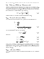
3.5 The IF Section
All mixer receivers at the 12m produce an intermediate frequency of 1.5 GHz. The IF
signal emerging from the receiver dewar must be further amplied and processed before
detection by the spectral line and continuum backend devices. A two-channel IF system
situated on the telescope performs this function. All the mixer receivers, except the 1mm
Array system, use this same processor; the switch from one receiver to another is done
remotely from the control room (see x3.4).
The incoming signal rst passes into an automatic leveling module. This device is
used in spectral line observations to keep the input signal to the lter banks at a constant
level, thus improving the performance of the lter banks. As this device will level out all
continuum signals, it is turned o by computer command when continuum observations are
underway. A manual switch in the control room can also turn o the device. After leaving
the Leveler Module, the signal is further amplied and ltered. It is then split into two
paths, one for spectral line signals and one for continuum. For continuum applications, the
1.5 GHz signal is detected and passed directly to the backend continuum signal processors.
The spectral line signal must be mixed down to the baseband frequencies at which
the lter banks operate. The IF Processor Module performs this function. The incoming
1500 MHz signal is rst upconverted to 2442 MHz. The mixer signal for this upconversion
originates with a tunable Fluke synthesizer in the control room. The frequency of the
mixing can be changed by small amounts and the two IF channels can be controlled by
separate Fluke synthesizers, if desired. This aords the observer some exibility in setting
up his observations. For example, the IF might be changed to get spectral lines in opposite
28
CHAPTER 3. INSTRUMENTATION
Table 3.4: 12m Filter Spectrometer Characteristics
Filter Bandwidtha Channels (Filters) per Bank Filter Banks Available
2 MHz
256
2
1 MHz
256
2
500 kHz
256
1
250 kHz
256
1
100 kHz
256
1
b
30 kHz
128
1
This is the FWHM channel width. See Appendix D for further details.
Series option only.
a NOTE:
b
sidebands to fall within the bandpass. One of the channels could also be oset in frequency
relative to the other. The primary restriction to these changes is that the spectral line
emission must fall within the 600 MHz bandpass of the rst IF amplier. Chapter 5,
Spectral Line Observing, provides a more detailed description of these options.
3.6 Spectrometers
3.6.1 Filter Banks
The 12m has eight lter spectrometers available for spectral line work. The multiplexer
will provide two spectra with a total number of spectral channels not in excess of 512.
Thus, it is always possible to record simultaneously the output of two lter banks. Except
for the 30 kHz bank, all of the lter banks have two independent 128 channel sections. You
can congure these banks in one of two ways. In the \series" option, the two sections are
placed end to end in frequency space, i.e., the 256 channels are sequential in frequency. In
the \parallel" mode, the two sections are used independently to accept dierent receiver
(polarization) channels. The series mode is appropriate for observations requiring a large
bandwidth. The parallel mode is useful for narrow band observations in which two dierent
spectral resolutions are needed. Additional discussion on the use of the lter banks is given
in Chapter 5.
Table 3.4 provides a list of the spectrometers. The resolutions listed are the lter half
power widths and their separations. The 2 MHz lter banks work at a center frequency
of 342 MHz and thus directly accept the output of the IF processor discussed above. The
other lter banks work at a center frequency of 150 MHz and require that the 342 MHz
input signal be further down-converted.
3.6.2 Millimeter Autocorrelator (MAC)
The Millimeter Autocorrelator (MAC) (MAC) is a correlation spectrometer with a digital
section similar in design to that used at the Green Bank Telescope (GBT). The full band-
3.7. COMPUTER EQUIPMENT
29
width for any given observation is pre-ltered through a set of anti-aliasing lters, and
then each IF is sampled in three levels and autocorrelated.
The 65536 spectral channels of the spectrometer can be divided among up to 8 independent IF channels. As such, it matches well with the 1mm Array receiver, as well as with
the dual-polarization channel, single beam receivers. The maximum useable bandwidth
of the instrument is 1200 MHz. Table 3.5 summarizes the currently available Millimeter
Autocorrelator (MAC) observing modes.
3.6.3 Continuum Backend
Continuum data at the 12m is acquired by a two channel, four phase digital backend
(DBE). The DBE can record two switch phases and two calibration phases. The calibration
phases can be generated by the synchronous emission of a noise diode, which is available
at 3 mm wavelengths only. The DBE also generates a signal/reference pulse to move the
subreector at a default switching rate of 1.25 Hz, so that each phase of a four phase
switching cycle lasts 125 ms. The DBE blanks the input signal (i.e. stops taking data)
while the subreector is in transition from one position to another. The blanking properties
are regularly adjusted by the 12m sta.
3.7 Computer Equipment
The 12 Meter Telescope computer system is composed of a network of Sun workstations. The telescope control and primary data analysis functions are controlled by a
dual-processor Sparcstation Ultra II. The control program is a C-language-based interface package called RAMBO. The RAMBO interface handles all of the functions of data
acquisition, including communication with the VxWorks device drivers which run the spectrometers, receivers, and other devices associated with a particular measurement. Most
major analysis packages are available on any of the telescope workstations.
30
CHAPTER 3. INSTRUMENTATION
Table 3.5: Millimeter Autocorrelator (MAC) Congurations
Bandwidth and Channels Useable Bandwidth and Channels1 2 Resolution
(MHz)
Channels
(MHz)
Channels
(kHz) (kHz)
800
800
400
400
200
200
100
100
2048
4096
4096
8192
8192
16384
16384
32768
600
800
800
400
400
200
200
100
100
1024
2048
2048
4096
4096
8192
8192
16384
600
600
300
300
150
150
75
75
600
300
300
150
150
75
75
600
2 IF Modes
1536
3072
3072
6144
6144
12288
12288
24576
390.6
195.3
97.6
48.8
24.4
12.2
6.1
3.0
781.2
390.6
195.3
97.6
48.8
24.4
12.2
6.1
768
1536
1536
3072
3072
6144
6144
12288
781.2
390.6
195.3
97.6
48.8
24.4
12.2
6.1
1562.0
781.2
390.6
195.3
97.6
48.8
24.4
12.2
4 IF Modes
8 IF Modes
800
512
384
1562.5 3125.0
800
1024
600
768
781.2 1562.0
400
1024
300
768
390.6 781.2
400
2048
300
1536
195.3 390.6
200
2048
150
1536
97.6
195.3
200
4096
150
3072
48.8
97.6
100
4096
75
3072
24.4
48.8
100
8192
75
6144
12.2
24.4
1 The useable bandwidth takes account of the 75% eÆciency of the analog lters.
2 NOTE: This is the frequency sampling interval, not the FWHM channel width,
for a given channel. The FWHM channel width is 2.0 times this value.
See Appendix D for details.
All values in this table refer to each IF.
Modes tagged with a are produced by dropping the last half of the lags.
Chapter 4
Tracking, Pointing, and Focus
4.1 Tracking Capabilities
The 12 Meter Telescope can track both stationary (sidereal) sources or fast moving sources
such as the Sun, Moon, planets, comets, or satellites (called \ephemeris objects"). The
positions of stationary sources may be entered into source catalogs by the observer or
directly into the on-line system by the operator. Stationary source positions may be given
as
Apparent equatorial positions (already precessed),
Equinox B1950 or J2000 equatorial positions, or
Galactic coordinate positions (lII, bII).
An example of the 12m catalog format is the following:
18:27:17.3
18:27:28.0
18:27:27.3
18:27:24.7
18:27:18.9
18:27:25.4
18:27:22.0
01:13:23.0
01:10:45.0
01:11:55.0
01:11:10.0
01:12:02.0
01:12:02.0
01:12:30.0
B1950
B1950
B1950
B1950
B1950
B1950
B1950
SERMM1
SERMM2
SERMM3
SERMM4
SERMM5
SERMM6
SERCTR
8.0
8.0
8.0
8.0
8.0
8.0
8.0
LSR
LSR
LSR
LSR
LSR
LSR
LSR
RAD
RAD
RAD
RAD
RAD
RAD
RAD
where
column 1 = right ascension (HH:MM:SS.S) or galactic longitude (DDD.DDDDD),
column 2 = declination (DD:MM:SS.S) or galactic latitude (DD.DDDDD),
column 3 = coordinate epoch (B1950, J2000, APPARENT, or GALACTIC),
column 4 = source name,
column 5 = source velocity,
31
32
CHAPTER 4. TRACKING, POINTING, AND FOCUS
column 6 = source velocity reference frame (LSR, HEL, GEO, or TOP), where
LSR = local standard of rest velocity reference frame,
HEL = heliocentric velocity reference frame,
GEO = geocentric velocity reference frame, and
TOP = topocentric velocity reference frame,
column 7 = source velocity type (RAD, OPT, or REL), where
RAD = radial velocity type,
OPT = optical velocity type, and
REL = relativistic velocity type,
The sky frequency equations corresponding to the above velocity types are given in Equations 5.4.
4.1.1 Ephemeris Objects
To track ephemeris objects (comets, asteroids, etc.), the control system requires three
positions, centered upon the present time. The tracking algorithm then makes a cubic
spline interpolation to determine the source position at the specic time of observation.
The observer must prepare a catalog in the correct format in order to observe ephemeris
objects other than the planets and the Moon. The basic format needed by the control
system is show below.
OBJ Hyakutake
VELFRAME LSR
VELTYPE RAD
#
# Ephemeris for Hyakutake, 0.000 H
#
D 45.7745 D 41.3975 J 50182.000720
D 45.7705 D 41.3822 J 50182.017387
D 45.7662 D 41.3670 J 50182.034053
D 45.7620 D 41.3517 J 50182.050720
D 45.7580 D 41.3363 J 50182.067387
D 45.7540 D 41.3212 J 50182.084053
D 45.7500 D 41.3058 J 50182.100720
D 45.7463 D 41.2907 J 50182.117387
D 45.7422 D 41.2755 J 50182.134053
D 45.7385 D 41.2603 J 50182.150720
D 45.7347 D 41.2452 J 50182.167387
D 45.7313 D 41.2300 J 50182.184053
9 APR 1996 to 23.700 10 APR 1996
0.00
0.00
0.00
0.00
0.00
0.00
0.00
0.00
0.00
0.00
0.00
0.00
55.84
55.86
55.89
55.91
55.93
55.94
55.95
55.96
55.97
55.97
55.97
55.97
33
4.2. TRACKING LIMITS
where the rst three lines are descriptors for the object name, velocity frame, and velocity
type. The next three lines are comments. Each column thereafter is dened as follows:
D 45.7745 = the topocentric right ascension in degrees.
D 41.3975 = the topocentric declination in degrees.
NOTE: You can also use a geocentric right ascension and declination in the last two
locations, but if you do you must enter the correct horizontal parallax (see below).
J 50182.000720 = the Modied Julian Date (mjd) of this record in the TT (Terrestrial
Time, which used to be called Terrestrial Dynamical Time, or TDT) system. Note
that TT = UTC + 63.184 sec after June 30, 1997.
0.00 = the horizontal parallax (the angle from you to the object to the center of the
earth in arcseconds). The horizontal parallax is zero in this case since we are using
topocentric coordinates. If one uses geocentric coordinates, the horizontal parallax
must be non-zero and is given by:
!
6378
:137
HP = arcsin
geocentric distance of object
55.84 = the topocentric velocity. Non-planets default to topocentric velocities. Plan-
ets default to geocentric positions and velocities.
After you create the ephemeris put it in a le with the extension eph in the observers
home directory { /home/obs/ini/comet.eph for example.
If you do not have an ephemeris generation program, we have a copy of the \TBEG4"
two body ephemeris generator program written by Don Yeomans which you can use. This
program will produce a 12m-format ephemeris le given a set of orbital elements. Contact
Je Mangum if you would like to use this program.
4.2 Tracking Limits
4.2.1 Elevation Limits
Mechanical limits constrain the movement of the telescope on both the azimuth and elevation axes. Under normal source-tracking operation, the control system software prevents
the telescope from moving into these limits. The telescope is also equipped with fail-safe
hardware limit switches that will turn the drive motors o and apply the brakes before
the telescope can be damaged. When the telescope reaches a lower elevation of 15.0Æ, it
begins to depress a safety spring on the elevation stop. Tracking can continue until the
elevation drive motor begins drawing excessive current; this usually occurs at an elevation
near 14.5Æ. A nal limit switch is tripped at 13.8Æ elevation.
The control computer will allow a source to be tracked up to an elevation of 90Æ. The
pointing equations diverge at the zenith, however, and elevations greater than 88Æ should
34
CHAPTER 4. TRACKING, POINTING, AND FOCUS
be strictly avoided during observations. For routine observations, we recommend that you
avoid elevations >80Æ if possible, since both tracking and pointing degrade in that range.
For maintenance purposes only, the telescope can be driven to an elevation of 92Æ before
tripping a nal limit switch.
4.2.2 Azimuth Limits
To prevent the over-wrapping of cables, the telescope has hardware and software azimuth
limits. The control system will not allow the telescope to rotate through 66.8Æ azimuth
to acquire or track a source. As they rise, sources with declinations between 27Æ and
38.75Æ will pass through 66.8Æ azimuth above 15Æ elevation. When a rising source reaches
an azimuth of 66.8Æ, the telescope will rotate 360Æ to re-acquire the source. The region
of the sky where azimuth transitions occur is displayed in Figure 4.1. If an integration
is in progress when the transition azimuth is reached, the integration is halted while the
telescope rotates around to re-acquire the source. The integration is resumed when the
source is reached again. If it is undesirable for this to happen, you should cease the
integration before reaching the transition azimuth.
4.3 Tracking Error Tolerance
The 12 Meter Telescope is vulnerable to tracking errors produced by wind gusts. The
tracking software has a provision for rejecting from the integration any data sample that
was taken with the telescope o source. The basic timing cycle of the 12m control system
is 100 milliseconds (0.1 sec). After each 100 ms interval, the system checks for error
conditions such as tracking errors or a loss of frequency phase lock. If an error condition
is detected, the data sample collected during the last 100 ms interval is not averaged with
the rest of the data.
You can choose how much tracking error you are willing to accept. This number is
called the \tracking tolerance" and is displayed on the on-line status monitor in the lower
left-hand corner under the heading \TOL". The 12m typically experiences 3{400 tracking
errors under calm conditions. The tolerance is usually not set to less than 500 for this reason.
Typical choices for the tolerance are 500 for 1.3 mm and shorter wavelength observations,
and 1000 for 2 and 3 mm observations. Figure 4.2 shows the amount of signal that is lost
by a given pointing error, expressed as fractions of a FWHP beamwidth.
4.4 Sequence of Position Computation Operations
The sequence of computer operations that is executed when seeking and then tracking a
source is as follows:
1. Input RA-DEC (B1950, J2000, or current epoch) or galactic (lII,bII).
2. If B1950 position, precess to current date. If galactic coordinates, rst precess to
epoch B1950 The precessed position of a source is computed only when the source is
rst accessed.
Figure 4.1: Local hour angle and declination versus azimuth and elevation for the 12m. The hatched region indicates the range
of source declination where the telescope will undergo a 360Æ azimuth transition while tracking a rising source.
4.4. SEQUENCE OF POSITION COMPUTATION OPERATIONS
35
36
CHAPTER 4. TRACKING, POINTING, AND FOCUS
Figure 4.2: Loss of signal due to pointing error.
3. If source is an ephemeris object, interpolate to current UT.
4. Do spherical coordinate conversion from RA-DEC to AZ-EL.
5. Add azimuth and elevation encoder corrections as computed from Equations A.1,
A.2, A.9, and A.10 (Appendix A).
6. Add azimuth and elevation pointing corrections.
7. Command telescope to the correct AZ-EL position.
8. Once every 10 seconds, go back to spherical coordinate conversion. Between loops,
extrapolate AZ and EL drive rates every 100 ms to compute positions.
4.5 Subreector Beam Throw
The 12 Meter Telescope is equipped with a nutating (chopping) subreector that is used
for beam-switched observations in both the spectral line and continuum modes. Other
observing modes, such as position switching, are made with the subreector locked in
37
4.5. SUBREFLECTOR BEAM THROW
place. Obviously, the throw position of the subreector, whether it is chopping or locked
in place, aects the pointing of the telescope. The current 12m subreector switches
only in azimuth, although mount misalignments may produce a small component in the
elevation direction (usually these are less than 1-200). The pointing equations for the 12m
are set up for 0 oset in subreector position, i.e. with the subreector axis aligned with the
electrical axis of the primary reector. When the subreector is oset so that the telescope
must be moved in the positive azimuth direction to bring the source into the beam, the
subreector is said to be in the \+BEAM". When the telescope must be moved in the
negative azimuth direction to acquire the source, at least with respect to the +BEAM, the
subreector is in the \ BEAM". Figure 4.3 illustrates this convention. Both the spectral
line and continuum backends are congured so that the +BEAM signal is positive and the
BEAM signal negative.
Pointing and
Electrical Axis
+BEAM
− BEAM
AZIMUTH ⇒
Figure 4.3: Subreector +Beam/ Beam conventions.
The control system software takes account of the subreector throw setting when positioning the telescope. The computer does not read the subreector setting automatically,
however; it depends upon the operator to manually set the throw value. The subreector
is physically set by turning two dials on the subreector control chassis. Default values of
subreector throw are stored in the computer: for example, 20 for 3 mm and 10 for 1
mm. You can check the beam throw by making a continuum cross-scan on a strong source.
Continuum mapping rows are explained in detail in Chapter 6.
38
CHAPTER 4. TRACKING, POINTING, AND FOCUS
4.6 Pointing
You are responsible for determining the residual azimuth and elevation pointing osets,
relative to the nominal telescope pointing. These osets are usually of the order 1000 { 2000
and often vary across the sky. In particular, the osets often show an elevation dependence.
The pointing of the 12m may drift over a period of several months by 1000 or so, and you
are cautioned not to assume that old pointing data are still valid. If a project requires
accurate pointing, observers should budget 5 - 10% of their total observing time to pointing
checks. High frequency projects, for which the FWHP of the main beam is 3000 or less,
obviously require more attention to the pointing.
You may perform pointing checks in either continuum or spectral line mode. Pointing
sources must have an angular brightness distribution that is compact compared to the
antenna beam. In addition, they must have well-determined positions and must be strong
enough to point on in a reasonable amount of time, e.g. 10 minutes or less. The best
pointing sources are the major planets Venus, Mars, Jupiter, Saturn, and Uranus, observed
in continuum mode. These sources have strong ux densities throughout the millimeter
band, although Uranus is faint at 3mm and longer wavelengths. To obtain complete sky
coverage, particularly north of the zenith, the planets must be supplemented with other
pointing sources. A tabulation of these sources and approximate ux densities at 3 and 1
mm is given in Table 4.1. This table includes the sources traditionally used at the 12m
together with sources found useful at the IRAM 30m telescope. The sources with no listed
ux density are on the order of 1 Jy in strength. It should be noted that the ux densities
of many of the extragalactic sources in the table can be highly time-variable. For an
up-to-date listing of measured 3mm uxes, see http://dopey.haystack.edu/cmva/quasar.list.
The spectral line emission from a number of sources can be used for pointing purposes.
Emission from rotational transitions of CO, HCN, and SiO are often strong enough and
angularly compact enough to provide good pointing results. A list of spectral line pointing
sources and their strong molecular emission lines are listed in Table 4.2.
4.6.1 Continuum and Spectral Line Five-Point Measurements
The ve-point mapping option is the standard observing technique for determining the
antenna pointing of the 12 Meter Telescope. Continuum ve-point measurements can also
be used to measure the ux density of a strong source with the highest precision, or the
ux density of a source whose position is not exactly known. The ve-point map consists of ve successive ON/OFF sequences (for continuum and beam-switched spectral
line measurements), or ve successive ON and OFF measurements (for position-switched
spectral line measurements), or ve successive ON measurements with one associated OFF
measurement (for total power spectral line measurements). The ve sequences or ON
measurements are positioned in azimuth and elevation relative to the nominal source position, as shown in Figure 4.4. The numbers identifying the positions give the time order
in which the sequences are taken. The oset for each position (\HP" in Figure 4.4), is a
selected oset (in arcsec) that is usually chosen to be close to half the HPBW of the telescope at the observing frequency. HP should be somewhat larger if the source is extended;
for a planet that is resolved by the beam, chose HP to be approximately the semi-diameter
4.6. POINTING
Table 4.1: Galactic and Extragalactic Continuum Pointing Sources
Source (B1950) Æ(B1950) S (3mm) (Jy) S (2mm) S (1mm) (Jy)
0003+380 00:03:22.3 +38:03:33
1.4
0048 097 00:48:10.0 09:45:24
1.8
0106+013 01:06:04.5 +01:19:01
0.9
0112 017 01:12:43.9 01:42:55
0119+041 01:19:21.4 +04:06:44
1.2
0133+476 01:33:55.1 +47:36:13
2.8
0135 247 01:35:17.1 24:46:09
1.3
0202+149 02:02:07.4 +14:59:51
3.7
W3(OH) 02:23:16.5 +61:38:57
3.8
0224+671 02:24:41.2 +67:07:40
0.8
0235+164 02:35:52.6 +16:24:04
1.5
0300+471 03:00:10.1 +47:04:34
1.5
3C84 03:16:29.6 +41:19:52
4.4
0336 019 03:36:59.0 01:56:17
2.1
NRAO150 03:55:45.3 +50:49:20
2.8
0415+379 04:15:02.1 +37:54:29
5.7
4.8
0420 014 04:20:43.5 01:27:29
2.9
0426 380 04:26:54.7 38:02:52
2.9
3C120 04:30:31.6 +05:15:00
1.5
0439+360 04:39:33.8 +36:01:15
1.1
0454 234 04:54:57.3 23:29:29
2.1
0458 020 04:58:41.3 02:03:33
1.9
0521 365 05:21:12.9 36:30:17
4.6
0528+134 05:28:06.8 +13:29:42
1.9
4.5
TAUA 05:31:30.0 +21:59:00
0552+398 05:52:01.3 +39:48:22
2.3
0605 085 06:05:36.0 08:34:20
1.7
0607 157 06:07:26.0 15:42:03
5.5
0642+449 06:42:53.0 +44:54:31
1.4
0716+714 07:16:13.0 +71:26:15
0.3
0727 115 07:27:58.1 11:34:53
1.2
39
40
CHAPTER 4. TRACKING, POINTING, AND FOCUS
Table 4.1: Galactic and Extragalactic Continuum Pointing Sources (continued)
Source (B1950) Æ(B1950) S (3mm) (Jy) S (2mm) S (1mm) (Jy)
0735+178 07:35:14.1 +17:49:09
0.5
0736+017 07:36:42.5 +01:44:00
3.2
0805 078 08:05:49.6 07:42:23
1.2
0814+425 08:14:51.7 +42:32:08
1.3
0820+560 08:20:53.2 +56:02:27
1.0
OJ287 08:51:57.3 +20:17:58
1.8
1.1
0923+392 09:23:55.3 +39:15:24
4.5
3.5
1034 293 10:34:55.8 29:18:27
0.6
1039+811 10:39:27.8 +81:10:24
0.4
1044+719 10:44:49.8 +71:59:27
1.5
1055+018 10:55:55.3 +01:50:04
2.0
1116+128 11:16:20.8 +12:51:07
0.3
1156+295 11:56:57.8 +29:31:26
1.7
3C273 12:26:33.2 +02:19:43
25.2
15.0
10
VIRA 12:28:17.6 +12:40:02
5.4
1244 255 12:44:06.8 25:31:28
1.8
3C279 12:53:35.8 05:31:08
14.9
12.9
1308+326 13:08:07.6 +32:36:40
1.5
1313 333 13:13:20.1 33:23:10
1.4
CENTA 13:22:31.7 42:45:30
9.4
1334 127 13:34:59.8 12:42:10
6.5
4.9
1354+195 13:54:42.1 +19:33:44
0.8
1413+135 14:13:33.9 +13:34:17
1.3
1418+546 14:18:06.2 +54:36:58
1.0
1502+106 15:02:00.2 +10:41:18
0.8
1504 167 15:04:16.4 16:40:59
1.1
1510 089 15:10:08.9 08:54:48
1.2
1514 241 15:14:45.3 24:11:23
1.2
1546+027 15:46:58.3 +02:46:06
2.0
2.7
1548+056 15:48:06.9 +05:36:11
2.1
1.3
1611+343 16:11:47.9 +34:20:20
2.1
1.1
4.6. POINTING
Table 4.1: Galactic and Extragalactic Continuum Pointing Sources (continued)
Source (B1950) Æ(B1950) S (3mm) (Jy) S (2mm) S (1mm) (Jy)
1622 253 16:22:44.1 25:20:52
0.4
0.5
1633+382 16:33:30.6 +38:14:10
1.6
1637+574 16:37:17.4 +57:26:16
1.1
1638+398 16:38:48.2 +39:52:30
1.0
3C345 16:41:17.6 +39:54:11
4.8
1.5
1655+077 16:55:44.0 +07:45:59
1.0
1657 261 16:57:47.7 26:06:29
1.8
NRAO530 17:30:13.5 13:02:46
5.8
8.4
1732+389 17:32:40.5 +38:59:47
1.0
1741 038 17:41:20.6 03:48:49
2.2
1749+096 17:49:10.4 +09:39:43
2.9
0.5
1803+784 18:03:39.2 +78:27:54
2.1
1807+698 18:07:18.5 +69:48:57
0.8
1823+568 18:23:14.9 +56:49:18
1.0
2.3
1828+487 18:28:13.5 +48:42:41
2.5
1921 293 19:21:42.2 29:20:26
10.3
7.3
1928+738 19:28:49.3 +73:51:45
2.8
1954+513 19:54:22.5 +51:23:46
1.1
CYGA 19:57:44.5 +40:35:46
1958 179 19:58:04.6 17:57:17
2.9
K3-50A 19:59:50.1 +33:24:19
6.5
2005+403 20:05:59.6 +40:21:02
1.5
2007+776 20:07:20.4 +77:43:58
1.5
2037+511 20:37:07.5 +51:08:36
3.0
DR21 20:37:14.3 +42:09:00
15.6
NGC7027 21:05:09.4 +42:02:03
5.2
2128 123 21:28:52.7 12:20:21
1.0
2134+004 21:34:05.2 +00:28:25
2.1
2145+067 21:45:36.1 +06:43:41
3.5
BLLAC 22:00:39.4 +42:02:09
1.9
2201+315 22:01:01.4 +31:31:06
3.0
2210 257 22:10:14.1 25:44:23
2.1
41
42
CHAPTER 4. TRACKING, POINTING, AND FOCUS
Table 4.1: Galactic and Extragalactic Continuum Pointing Sources (continued)
Source (B1950) Æ(B1950) S (3mm) (Jy) S (2mm) S (1mm) (Jy)
2216 038 22:16:16.4 03:50:41
1.2
3C446 22:23:11.1 05:12:18
4.0
2230+114 22:30:07.8 +11:28:23
3.7
2234+282 22:34:01.7 +28:13:23
1.2
2243 123 22:43:39.8 12:22:40
2.3
3C454.3 22:51:29.5 +15:52:54
6.3
2255 282 22:55:22.3 28:14:22
2.4
NGC7538 23:11:36.7 +61:11:50
2.1
2318+049 23:18:12.1 +04:57:23
1.1
CASA 23:21:11.0 +58:32:48
2345 167 23:45:27.7 16:47:53
2.2
of the source.
To make a ve-point map proceed as follows:
Continuum Five-Point:
1. Select an appropriate source to point on, such as a planet or other strong continuum source.
2. Using the pointing charts, make an initial guess for the azimuth and elevation
pointing osets.
3. Ask the operator to setup for a continuum ve-point measurement on the chosen
source. The operator will set the integration time per sample and the number of
OFF{ON{ON{OFF sequence pairs to measure on the source. For the stronger
sources, 5 seconds and 1 pair is suÆcient. For the weaker sources, 10 seconds
and 2 or 3 pairs may be needed. If the source is somewhat extended, ask the
operator to set the grid spacing to be the semi-diameter of the source. All other
parameters will default to reasonable values. Once everything is set, ask the
operator to start the measurement.
Spectral Line Five-Point:
1. Select an appropriate source. The source listing in Table 4.2 is by no means
all-inclusive, but if another source is used, take care that it is really suitable for
use as a pointing source. In particular, it should have an angular size that is
smaller than, or at least comparable to the antenna beam size and possess an
accurately known position.
Source
R Scl
Mira
IK Tau
GL 618
Ori IRc2
U Ori
GL 865
VY CMa
R Leo
IRC+10216
CIT 6
V Hya
R Hya
W Hya
U Her
IRC+20326
VX Sgr
IRC+20370
W Aql
Cyg
V Cyg
NML Cyg
01:24:39.9
02:16:49.0
03:50:43.7
04:39:33.8
05:32:47.0
05:52:50.9
06:01:17.5
07:20:54.7
09:44:52.2
09:45:14.8
10:13:11.0
10:49:11.3
13:26:58.4
13:46:21.1
16:23:34.7
17:29:42.0
18:05:03.2
18:39:41.7
19:12:41.6
19:48:38.5
20:39:41.3
20:44:33.8
(B1950)
Table 4.2: Spectral Line Pointing Sources
CO
HCN
SiO
1
Æ (B1950) VLSR (km s ) TR (1 ! 0) TR (2 ! 1) TR (1 ! 0) TR (2 ! 1)
32:48:05
18.0
1
?
?
N.E.
03:12:12
47.0
1
3 (v)
11:15:30
35.0
0.5
5 (v)
36:01:15
21.0
1
N.E.
05:24:24
4.0
20:10:05
39.0
1 (v)
07:26:03
42.0
0.5
N.E.
25:40:12
24.0
11:39:40
1.0
0.1
8 (v)
13:30:41
26.0
8
12
N.E.
30:49:17
2.0
2
2
N.E.
20:59:03
18.0
0.5
N.E.
23:01:23
1.0
28:07:08
40.0
19:00:16
14.0
1 (v)
17:47:36
5.0
0.5
N.E.
22:14:06
6.0
10.0
17:38:16
1.0
0.8
1
N.E.
07:08:08
25.0
1.0
N.E.
32:47:11
10.0
0.7
1.5
5 (v)
47:57:44
13.0
1
1
N.E.
39:55:57
0.0
4.6. POINTING
43
44
CHAPTER 4. TRACKING, POINTING, AND FOCUS
+EL Point
Grid Size ("HP")
1
−AZ Point
4
+AZ Point
5
3
Center Point
2
−EL Point
El
Five Point Mapping Scan
Layout and Order of Measurements
Figure 4.4: Five point mapping scan sequence.
Az
4.6. POINTING
45
2. Ask the operator to setup for a spectral line ve-point measurement on the
chosen source. Set the integration time per sample, the number of ON/OFF
pairs to measure on the source, the number of scans per calibrate, and for a
total power ve-point the ON and OFF integration time. Depending on the
source size, you may also have to set the grid spacing appropriately. All other
parameters will default to reasonable values.
3. Choose an azimuth oset angle for the reference, to be used for position switching.
4. Using the pointing charts, make an initial guess for the azimuth and elevation
pointing osets.
5. Ask the operator to start the measurement.
To process these measurements, there are a number of condar and line procedures
available.
4.6.1.1 Continuum Five-Point Analysis
Continuum ve-point measurements are processed automatically by the on-line dataserver.
The results from these on-line ts are sent automatically to the operator for entry into the
control system. To process a continuum ve-point measurement manually, use the condar
resident procedure ve, which can be abbreviated as f. You can look at the results for each
channel separately by using the command
Condar > scan number f
Channel 1 is selected by specifying subscan number .01, while channel 2 is selected with
subscan .02. The display (Figure 4.5) provides the observer with the best-t positional
osets in azimuth and elevation, along with the estimated peak ux density of the source,
both for a constrained t of Gaussian half-width HP and an unconstrained solution. The
optimum pointing osets (labeled corrected offsets) are also printed, assuming the
given position of the source to be correct.
4.6.1.2 Spectral Line Five-Point Analysis
The display of the map and the t for pointing osets is somewhat more involved than for
a continuum ve point. There is a standard line procedure which processes all types of
spectral line ve-point measurements. To process a measurement, within line type:
Line> center scan number fivel1 (for channel 1)
Line> center scan number fivel2 (for channel 2)
You will be asked some questions by the routine:
{ This question is asked only if the
data were taken in series mode. If the question is answered \yes", the routine averages
the rst and second lter bank to improve sensitivity. You should answer \yes" only
if you are reducing the rst lter bank; you will usually not need to reduce the two
lter banks separately if averaging the two. If the data were taken in parallel mode,
the two polarization channels in each lter bank are automatically averaged.
AVERAGE THE TWO RECEIVERS? (1=YES, 0=NO)
CHAPTER 4. TRACKING, POINTING, AND FOCUS
Subreflector Beam Throw
Input AZ Pointing Correction
Input EL Pointing Correction
AZ Flux
RMS of Flux Measurement
Best Fit Location for Pointing Source
Fitted FWHP Beam Widths
in AZ and EL
46
New Pointing Offsets
Figure 4.5: Continuum Five-Point Analysis Example
4.6. POINTING
47
Figure 4.6: Display of each scan produced by the line procedure vel.
{ The observer must dene baseline tting and spectral line integration regions for this routine. If these
regions have already been accurately set, as, for example, in a ve-point of the same
source performed immediately prior to the present one, you can answer \yes" and
speed up the reduction process considerably. If you answer \no", the spectrum at the
center of the map is displayed on the screen, and the question ENTER # OF BL SEGS
is printed. This part of the f routine is the same as the bset procedure. The observer
must enter the number of baseline segments to be used to t a least-squares baseline.
[NOTE: The order of the t is determined by whatever nt is set to (the default is 1 {
see the line data reduction manual for a description of the baseline tting facilities).]
When the number of segments to be t is entered, the graphics crosshairs appear
and you must mark o the two ends of each segment with the crosshairs (move the
crosshairs to the desired position and strike any mouse button). When this operation
is nished, the baseline is removed from the center spectrum and the spectrum is replotted. The prompt ENTER INTEG. REGIONS is printed and the crosshairs reappear.
You should then mark o the two velocity/frequency extremities of the spectral line
(or whatever region you wish to integrate over).
USE OLD BASELINE & INTEG. REGIONS? (1=YES, 0=NO)
{ If you answer \no", the map and the t for
new osets are printed out. If you answer \yes" each scan of the map, with baselines
removed, is displayed on a single plot, one spectrum on top of the other (see Figure
4.6).
DISPLAY EACH SCAN? (1=YES, 0=NO)
48
CHAPTER 4. TRACKING, POINTING, AND FOCUS
{ If you approve of the ts, answer 1 and the
map and t for new osets will be displayed. An example of the ve-point map with
explanatory annotations is given in Figure 4.7.
TYPE 1 TO CONTINUE OR 0 TO STOP
4.6.2 Pointing Model Equations
In addition to coordinate conversions, the telescope tracking program incorporates pointing
corrections. The pointing corrections take into account resolver zero osets, dierences
between electrical and mechanical axes, axis tilt, etc. The coeÆcients of the pointing model
equations are determined during dedicated optical and radio pointing source measurements
several times during the observing season. The pointing models used for the 12m are
described in detail in Appendix A.
4.6.3 Pointing Data Analysis Program
Each time a continuum ve-point measurement is made, the on-line data server performs
a t to the results and writes them to a permanent le for later analysis. A program called
gpoint is available on any of the mountain workstations for display and analysis of the
recent pointing history of the telescope.
To start the program, type gpoint from any login prompt. gpoint is menu-driven, so
you need only select the appropriate entries in each menu to congure the data selection
and display parameters to suit your needs. An example of a gpoint plot is given in Figure
4.8.
4.7 Focus
4.7.1 Axial Focus
To bring the incident radiation to a focus at the receiver feed horn, the subreector of the
12m may be moved in and out along the electrical axis of the telescope. The focus exhibits
an elevation dependence which is automatically corrected by the control system computer,
according to the equation
F (E ) = F0 + 2:8 sin(E )
(4.1)
where F (E ) is the focus setting in millimeters, E is the elevation, and F0 , the subreector
focus setting at 0Æ elevation, is to be determined by the observer. F0 is given in millimeters, and larger values of F0 represent greater distances between the dish surface and the
subreector.
An automatic procedure called a focalize (this word really is in the dictionary!) will
determine the best value for F0. An analysis routine of the same name exists in condar
and line for displaying and tting the results. Instructions for performing a focalize are
given in x4.7.2.
4.7. FOCUS
Input AZ Pointing Correction
Input EL Pointing Correction
AZ Intensity of Channel 1
AZ Intensity of Channel 2
Best Fit Location for Pointing Source
Fitted FWHP Beam Widths
in AZ and EL
New Pointing Offsets
49
Figure 4.7: Spectral line ve-point analysis example.
CHAPTER 4. TRACKING, POINTING, AND FOCUS
50
Figure 4.8: GPOINT display example. Each pointing source is indicated by a unique symbol, while the arrow on each symbol
indicates whether the source was rising or setting.
4.7. FOCUS
51
4.7.2 Determining the Axial Focus
The axial focus of the telescope should be checked occasionally during an observing run.
It is often most convenient to make a focus check after a continuum ve-point pointing
measurement since both measurements use the same kinds of sources (strong continuum
point sources). It is particularly important to check the focus after nightfall and daybreak.
Focusing is performed via the focalize procedure. This steps the radial distance of the
subreector from the telescope vertex through seven positions centered on the nominal
best setting (F0). Larger values of F0 represent greater distances between the dish surface
and the subreector. The incremental movement between positions (WL) is set to half of
the observing wavelength by default, but can be set by the observer.
Perform a focalize as follows:
1. Choose as bright a continuum source as possible. The planets Jupiter, Venus and
Saturn are ideal. If the source is extended relative to the telescope main beam, the
accuracy of the focalize will be diminished, however.
2. Make a ve-point map of the source to optimize the antenna pointing (see x4.6.1).
3. Reasonable default values for the axial subreector position (F0) have been assigned
to each receiver, but, if you nd it necessary you can give the operator a value for
F0.
4. The default integration time per sample is 5 seconds, but if you are performing a
focalize measurement on a weak source, you may need to increase this to 10 { 15
seconds.
5. If you are satised with the setup, ask the operator to start the measurement.
Focalize measurements are processed automatically by the on-line dataserver, the results of which are sent automatically to the operator for entry into the control system. To
reduce the focalize in condar use the commands,
Condar > scan number focalize
where each channel is selected by specifying either subscan .01 for channel 1 or .02 for
channel 2. The output from the focalize procedure is shown in Figure 4.9. The t should
be smooth and \quasi-Gaussian". (If not, repeat the focalize. Increase the value of WL
if you think this is necessary.) The display will give a best-t value for F0. Where
appropriate, you should average the values for the two channels.
4.7.3 Lateral Focus
The position of the subreector for optimum gain shifts in the elevation direction, with
changing elevation angle. The change in antenna gain produced by this eect is not
signicant at 3mm wavelengths but could be as much as 20% or more at 1.3mm and
shorter wavelengths. The 12m is equipped with lateral \north-south" and \east-west"
translation stages at the prime focus to eliminate this loss in antenna gain. The computer
is able to automatically control the positioning of these stages, simultaneously applying
CHAPTER 4. TRACKING, POINTING, AND FOCUS
52
Input Radial Focus Value
Focus Step Size Between Measurements
Best Fit Gaussian
Measurements at Discrete Foci
are indicated by a +
Figure 4.9: Focalize display example.
4.7. FOCUS
53
an appropriate correction to the telescope pointing in elevation and azimuth, respectively.
This correction to elevation pointing is 31.500/mm (which is the prime focus \plate scale"
derived in Appendix G) of movement in the north-south focus or east-west focus stages.
In the future, the coeÆcients necessary to control the movement of the north-south and
east-west translation stages will be installed in the computer and applied automatically. At
this time, the north-south and east-west translation stages can be set to a given position,
but are usually left xed in this position. Automatic procedures for tting for maximum
north-south or east-west gain, called nsfocal and ewfocal are available. These routines
operate analogously to the focalize procedure. Normally, only sta astronomers use these
procedures; we do not recommend that observers spend time trying to optimize this further.
54
CHAPTER 4. TRACKING, POINTING, AND FOCUS
Chapter 5
Spectral Line Observing
5.1 Startup Checklist
Once the scientic goals of the observing session are clearly in mind, you must decide upon
the equipment and observing techniques to be used. The decisions to be made and the
options are listed below.
Sideband Choice: For double sideband observations, care must be taken in choosing
the placement of the image sideband.
Spectrometer Conguration: Filter bank spectrometers with several dierent resolutions are available. The observer must choose which to use and how they should be
congured (the parallel or series option). The Millimeter Autocorrelator (MAC) ,
which has numerous resolution and bandwidth options, is also available.
Observing Mode: Choices are
Total Power Scans { ON and OFF total power spectra are recorded separately for
later processing into nal spectra. The observer may take several ON scans for
each OFF.
Position Switching { The telescope moves between an oset, or OFF, position (in
relative or absolute coordinates) and a source, or ON, position. The spectrum
is recorded as a ratio of (ON { OFF)/OFF.
Frequency Switching { The local oscillator is shifted by several MHz at a rate of
1.25, 2.5, or 5.0 Hz. The spectrum is recorded as a ratio of (SIG { REF)/REF.
Beam Switching plus Position Switching { The subreector is chopped at a rate of
1.25 to 5.0 Hz, and the telescope is repositioned at a prescribed rate (typically
every 30-90 seconds). The spectrum is recorded as (ON { OFF).
Grid Mapping { Total power or absolute position or frequency switched data are
acquired while the telescope moves to user-specied spatial positions.
On The Fly Mapping { Total power data are acquired every 0.1 seconds while the
telescope is driven continuously over a specied map eld.
55
56
CHAPTER 5. SPECTRAL LINE OBSERVING
Prior to the start of observations, you should make a rough
budget of observing time requirements. In addition to the integration time on the
program sources, you should allow time for \overhead" items such as telescope movement, and pointing and calibration tests.
Before beginning program observations, check the telescope pointing and focus. A
few observations of test sources are also advisable. These observations are discussed in
Chapters 2, 4, and 6.
Observing Time Budget:
5.2 Sideband Choice
All of the 12m receivers operate by default in a single sideband (SSB) mode and require
upper sideband (USB) operation. For the 2 and 3mm receivers, it is possible to observe
DSB. Equipment constraints, such as the tuning range of the local oscillator or the receiver,
may sometimes determine the sideband used in DSB mode. Other times, the presence of
telluric lines steer the choice (see Figure 6.1). When using DSB mode, make the sideband
choice with care.
The primary things to watch out for when choosing the sideband conguration for
a DSB measurement is the presence of \contaminating" lines from the image sideband.
Consult a good tabulation of spectral lines such as the Lovas Catalog (F. J. Lovas, J.
Phys. Chem. Ref. Data, 15, 251, 1986) to see what spectral lines are present in both the
signal and image sidebands. If an image line is too close to the program line in the signal
sideband, a small local oscillator shift will usually cure the problem (the frequency axes
run oppositely for the upper and lower sidebands). One can also make small adjustments
in the IF to change the placement of lines from the two sidebands. Sometimes, lines from
the image sideband can be used to advantage for calibrations or system checks.
With a slight rearrangement of Equation 3.4, we can write the expression for the sky
frequency as a function of the LO frequency settings
= m (Nfsyn + flock ) jfIF
(5.1)
where fsyn is the synthesizer frequency, fsky is the sky frequency of the emission (the rest
frequency with Doppler corrections), j = +1 for lower sideband and 1 for upper sideband,
fIF is the IF frequency (1.5 GHz by default), m is the factor by which the LO frequency is
multiplied before injection into the mixer, flock is the the phase lock loop oset frequency
(100 MHz), and N is the synthesizer harmonic. The Doppler correction is determined by
the choice of velocity type (see Chapter 4).
fsky
fsky (RAD)
=
frest
1
vobject + vantenna
c
frest
= 1 + vobject
+vantenna
c
v
u
u 1 vobject +cvantenna
fsky (REL) = frest t
1 + vobject +cvantenna
fsky (OP T )
!
(5.2)
(5.3)
(5.4)
5.3. SPECTROMETERS
57
where vobject and vantenna are the object and antenna velocities relative to the local standard
of rest and c is the speed of light.
5.3 Spectrometers
Two spectrometer systems are available at the 12m: a suite of analog lter banks and a
Millimeter Autocorrelator (MAC), which is a digital correlation spectrometer.
5.3.1 Filter Banks
Most of the analog lter banks have 256 channels each. The lters are integrated, multiplexed, and recorded by the control computer every 100 milliseconds. A total of 512
channels can be recorded at a time, which means that two lter banks can be used for each
scan. The lter spectrometers available and the ways in which they can be congured are
described below. Table 5.1 lists the characteristics of the 12m lter banks
5.3.1.1 The Parallel/Series Option
Most of the 256 channel lter banks can be split into two 128 channel sections that can be
fed with independent IF signals. When a lter bank is split into two sections, the bank is
said to be in a parallel conguration. Each polarization channel of the receiver feeds half
of a lter bank in this conguration. The advantage of this mode is that the two halves of
the lter bank can be averaged to produce improved signal-to-noise in the nal spectrum.
The disadvantage of this mode is that the total bandwidth is cut in half. Observers of
narrow Galactic lines typically choose the parallel option, and use two lter banks with
dierent resolutions.
Observations that require larger bandwidths, such as CO from other galaxies, usually
choose the series mode. In the series mode, the two lter bank halves are used end-to-end
to analyze a single input IF signal. A typical observing mode might be to use one of the
1 MHz lter banks for polarization 1 and the other for polarization 2. The two banks can
be averaged in software to improve the signal-to-noise of the nal spectrum. Figure 5.1 is
a diagram showing how the parallel/series option works.
5.3.1.2 Bad Channel Elimination
At times, certain channels in the lter banks are defective. You can identify these \bad"
channels by examining the output of a vane calibration cycle, which is called the gains.
Vane calibration is described in detail in x5.6.1. Bad lter channels usually appear as spikes
in the gains and will often cause scaling problems in the nal spectrum if not eliminated.
You can display the gains with the line data reduction program. To nd the bad channels,
perform a calibration scan and type g1 to display the rst lter bank and g2 to display
the second bank. If bad channels exist, type the command badch. You will be asked to
enter the number of bad channels. After doing so, the crosshairs will appear on the screen.
Move the vertical crosshair to each bad channel and select any mouse button. When all
the bad channels have been entered, the program will give a report of the channel numbers.
CHAPTER 5. SPECTRAL LINE OBSERVING
58
This is the FWHM channel width. See Appendix D for further details.
Table 5.1: 12m Filter Bank Characteristics
Filter Resolutiona Channels per Bank Filter Banks Available Parallel/Series Option Hardware Center Channel (Par/Ser)
2 MHz
256
2
yes
64.5/128.5
1 MHz
256
2
yes
64.5/128.5
500 kHz
256
1
yes
64.5/128.5
250 kHz
256
1
yes
64.5/128.5
100 kHz
256
1
yes
64.5/128.5
30 kHz
128
1
no
65
a NOTE:
59
5.3. SPECTROMETERS
Series Filter Bank Configuration Option
Rx1
Rx2
256 Channels
256 Channels
Filter Bank 1
Filter Bank 2
Parallel Filter Bank Configuration Option
Rx1
128 Channels
128 Channels
Filter Bank 1
Rx2
128 Channels
128 Channels
Filter Bank 2
Figure 5.1: The lter bank parallel and series congurations.
60
CHAPTER 5. SPECTRAL LINE OBSERVING
Give these numbers to the operator. Up to 16 bad channels can be eliminated, but rarely
more than 5 channels out of 512 will be bad. It is also possible to eliminate blocks of 16
channels, but this is seldom necessary. If blocks of 16 channels are bad, notify the Friend
of the Telescope.
Once the operator has entered the bad channels, he will perform another vane calibration cycle to set the bad channels to 1:0 10 20, which is the agged channel value. On all
subsequent spectra, those channels will be agged. These bad channels can be eliminated
in reduction software by using the replace command (see the line manual).
5.3.1.3 Frequency Osets
Given the broad-band tunability of the 12m receivers, one can shift the rest frequency measured by the lter banks by specifying a frequency oset to be added to the rest frequency.
Osets as large as the entire bandwidth of the receiver (300 MHz) are possible. Filter
bank osetting is most often used in conjunction with the 4IF Millimeter Autocorrelator
(MAC) mode (see x5.3.2.1 for further information).
5.3.2 Millimeter Autocorrelator
The Millimeter Autocorrelator (MAC) oers a number of bandwidth and resolution modes,
listed in Table 5.2. Most general single-beam dual-polarization measurements are done using the congurations with 2 IF's. The 8 IF modes are designed for use with the 1mm Array
receiver. The 4IF Millimeter Autocorrelator (MAC) mode is a special-purpose observing
mode allowing the measurement of two frequencies each at two polarizations simultaneously.
5.3.2.1 The 4IF Observing Mode
One of the more eÆcient observing modes available at the 12m involves the use of the 4IF
conguration of the Millimeter Autocorrelator (MAC) in conjunction with the frequency
osetting capabilities of the lter banks. Within the IF modules which feed the receiver
signals to the Millimeter Autocorrelator (MAC) there are oscillators which can shift the
input receiver signals by 300 MHz in 5 MHz steps. Since these oscillators are independent
of the Fluke synthesizers which provide the frequency osetting capabilities of the lter
banks, it is possible to measure spectra at three separate frequencies within the 600 MHz
bandwidth of the receiver (assuming both mixers are tuned to the same frequency). A
graphical description of this mode is shown in Figure 5.2.
To given a practical example, say I want to simultaneously measure the H2CO emission from the 303 ! 202 and 322 ! 221 transitions at 218222.192 and 218475.632 MHz,
respectively. These two frequencies are separated by 253.440 MHz, which would restrict
my choice of backends to the 2MHz lter banks in parallel and the 600 MHz Millimeter
Autocorrelator (MAC) mode. Since I want to look at galactic sources with narrow lines,
this wide-band modes are not acceptable. To use the 4IF mode to measure both transitions
simultaneously, I would
61
5.3. SPECTROMETERS
Table 5.2: Millimeter Autocorrelator (MAC) Congurations
Bandwidth and Channels Useable Bandwidth and Channels1 2 Resolution
(MHz)
Channels
(MHz)
Channels
(kHz) (kHz)
800
800
400
400
200
200
100
100
2048
4096
4096
8192
8192
16384
16384
32768
600
800
800
400
400
200
200
100
100
1024
2048
2048
4096
4096
8192
8192
16384
600
600
300
300
150
150
75
75
600
300
300
150
150
75
75
600
2 IF Modes
1536
3072
3072
6144
6144
12288
12288
24576
390.6
195.3
97.6
48.8
24.4
12.2
6.1
3.0
781.2
390.6
195.3
97.6
48.8
24.4
12.2
6.1
768
1536
1536
3072
3072
6144
6144
12288
781.2
390.6
195.3
97.6
48.8
24.4
12.2
6.1
1562.0
781.2
390.6
195.3
97.6
48.8
24.4
12.2
4 IF Modes
8 IF Modes
800
512
384
1562.5 3125.0
800
1024
600
768
781.2 1562.0
400
1024
300
768
390.6 781.2
400
2048
300
1536
195.3 390.6
200
2048
150
1536
97.6
195.3
200
4096
150
3072
48.8
97.6
100
4096
75
3072
24.4
48.8
100
8192
75
6144
12.2
24.4
1 The useable bandwidth takes account of the 75% eÆciency of the analog lters.
2 NOTE: This is the frequency sampling interval, not the FWHM channel width,
for a given channel. The FWHM channel width is 2.0 times this value.
See Appendix D for details.
All values in this table refer to each IF.
Modes tagged with a are produced by dropping the last half of the lags.
CHAPTER 5. SPECTRAL LINE OBSERVING
MAC Spectrometer 4IF Mode Configuration
Rx1
Filter Bank Offset
Filter Bank Offset
ν1
Filter Bank
62
Rx2
ν2
MAC Spectrometer
Offsets
MAC Spectrometer
IF 11
ν3
MAC Spectrometer
IF 12
ν1
Filter Bank
ν2
MAC Spectrometer
Offsets
MAC Spectrometer
IF 13
Figure 5.2: Millimeter Autocorrelator (MAC) 4IF mode conguration.
ν3
MAC Spectrometer
IF 14
5.4. OBSERVING MODES
63
1. Tune the receiver to a frequency midway between the two rest frequencies, which in
this case is 218348.912 MHz.
2. Set the lter bank oset so that I can measure the 303 ! 202 transition, which would
be 218348.912 218222.192 = 126.720 MHz.
3. Set the two Millimeter Autocorrelator (MAC) osets so that IF's 11 and 13 receive
the 303 ! 202 transition and IF's 12 and 14 receive the 322 ! 221 transition. Since
the Millimeter Autocorrelator (MAC) osets must be in 5 MHz steps, I would set
these osets to 125 MHz. The center frequency for IF's 11 and 13 would then be
218348.912 125.0 = 218223.912 MHz, while the center frequency for IF's 12 and
14 would be 218348.912 + 125.0 = 218473.912 MHz.
5.4 Observing Modes
There are six primary spectral line observing modes are available at the 12m. The attributes and applications of each are described in detail below. Signal processing and
calibration for each mode are described in x5.6.
5.4.1 Total Power ONs and OFFs
Two observing procedures, called tpon and tpo, are available for recording total power
spectral line scans. The two procedures are identical, except that tpon tracks the ON
(source) position and tpo tracks the OFF (reference) position. You must execute the
procedures manually, one scan at a time. As such, these procedures are mainly used for
diagnostic purposes. To use tpo and tpon, follow this prescription:
Provide the operator with the following setup information:
1. The source catalog and the source name (the ON position).
2. The (AZ,EL) pointing corrections and the reference oset position (OFF). The
oset may be specied in AZ and EL or in RA and DEC.
3. The integration time of the scan in seconds (the scan will have only one sample,
i.e., repeats does not apply to TPN or TPF scans).
Have the operator perform a vane CALIBRATE, a TPF (the OFF scan), and a TPN (the
ON scan) in that order. The scan numbers of the CALIBRATE and TPF will be stored
in the header of the TPN scan for use in data processing.
To look at either the TPF or TPN scans, type
Line> scan# f
Line> scan# s
to choose either the rst or second lter bank, respectively. The displayed scan will
be a total power bandpass. Unless the band contains a very strong spectral line, you
64
CHAPTER 5. SPECTRAL LINE OBSERVING
will probably not be able to see any lines. To display a nal spectrum, formed from
the ratio (ON{OFF)/OFF * CAL, type
Line> install ton
Line> scan# ton
(Note that you only need to install the procedure once per session). The ton
procedure will use the last CALIBRATE and TPF scan to form the spectrum.
5.4.2 Position Switching
Position switching, called the PS mode, is the most common and reliable observing mode
at the 12m for general spectral line observations. It involves considerable overhead in
telescope movement and requires that equal time be spent in the ON and OFF source
positions, but the data quality is usually good. In this mode, the telescope moves between
the ON position and a relative OFF position, which may be specied in either azimuth and
elevation, or right ascension and declination osets. Usually the oset is in azimuth, so
that the ON and OFF positions are taken at about the same airmass. The best rejection of
the atmosphere and the best spectral baselines are achieved with small angular switches.
Choose the smallest switch possible, so long as you are condent that the OFF position is
free of source emission.
PS data recorded on disk is a nal spectrum formed from the ratio (ON{OFF)/OFF,
where the ON and OFF data are total power samples. In contrast to the total power
observing modes TPON and TPOFF, the ON and OFF samples are not saved as separate
scans for independent processing. Although the PS mode oers less exibility in processing
data than do the total power modes, it also reduces the total volume of data and makes
processing easier.
To reduce telescope movement and provide the best compensation for polynomial drifts
in atmospheric emission, choose the number of OFF{ON pairs to be a multiple of 2. The
observing cycle will then be repeats of an OFF{ON{ON{OFF pattern characterized by a
Walsh function (see Appendix E). Each ON or OFF is called a sample and each OFF{ON
pair is called a repeat. The observer must tell the operator how long to integrate for
each sample (the default is 30 seconds) and how many repeats per scan, or alternatively,
the total length of the scan in minutes. A typical scan might be 6 minutes long, with 30
second samples (meaning 6 repeats). You can, of course, vary the length of the scan to
suit your own needs. Each ON{OFF pair can be edited individually with the line program
(see Record Editing in the supplement to the line manual). The operator can issue the
command to take scans one at a time, or can set the system into an automatic data-taking
loop. Figure 5.3 shows an example of a spectrum produced by a PS scan.
The parameters of a PS scan that you must give to the operator are
The relative oset position, which may be specied in either (AZ, EL) or (RA, DEC)
coordinates.
The integration time for an individual sample (ON or OFF). 30 seconds is the default.
5.4. OBSERVING MODES
Rest Frequency (MHz)
Total Integration Time
LO Synthesizer Frequency (kHz)
*
Tsys
Velocity Resolution (km/s)
Filter Bank Resolution (kHz)
65
Figure 5.3: Position switched spectral line scan analyzed in the unipops program.
66
CHAPTER 5. SPECTRAL LINE OBSERVING
The number of ON/OFF pairs (repeats) per scan (can be specied to the operator as
the total length of the scan).
The number of scans to be performed for every calibration measurement.
5.4.3 Absolute Position Switching
Absolute position switching, called the APS mode, is useful when observing in complex
emission regions where it is diÆcult to nd an emission-free reference position. In such
cases, position switching with (AZ,EL) osets can be dangerous because rotation of the
parallactic angle as the source is tracked across the sky may cause emission to rotate into
the reference beam. You will want to search for an emission-free position as close to the
source position as possible, and use this as the reference position. If you wish, you can
compute the (RA,DEC) osets to this position and use ordinary position switching. Most
observers nd it most convenient, particularly for future observations, to enter the absolute
(RA,DEC) coordinates of the reference position and use the absolute position switching
observing mode.
APS is identical to ordinary position switching except that the switching is done between two positions absolutely specied by their celestial coordinates. The reference (OFF)
position should be given a dierent name from the signal (ON) position and is best placed
in a dierent source catalog from the signal position. Data taking and calibration options
are the same as for ordinary position switching.
The parameters of an APS scan that you must give to the operator are
The name of the source (ON) position and catalog which contains it;
The name of the reference (OFF) position and its catalog;
The integration time for each sample (ON or OFF). 30 seconds is the default;
The number of repeats of an ON{OFF pair or the total integration time of the scan;
The number of scans between each vane calibration, if that calibration method is chosen.
5.4.4 Frequency Switching
The frequency switching observing mode has two primary uses: to increase the on-source
integration time through \in-band" switching and to alleviate the problem of nding an
emission-free reference position when observing in a (spatially) complex emission region.
It also entails less system overhead than most other observing modes. In this mode, called
an FS observation, a reference spectrum is obtained by shifting the center frequency of
the signal spectrum. In principle, this can be done by switching the frequency of the LO
or an IF oscillator; at the 12m, the former is generally used. If the frequency shift is
small enough, the spectral line will appear in both the signal and reference spectra. When
the resultant spectrum is formed, the line will appear twice,
p once in emission and once in
absorption. The spectrum can be \folded" to obtain a 2 improvement in signal-to-noise.
With this technique, which is called \in-band" or \overlapped" frequency switching, you
5.4. OBSERVING MODES
67
are eectively observing on-source all the time. Figure 5.4 shows an example of a spectrum
produced by a FS scan.
The primary drawback of frequency switching is that the spectral baselines are generally
not as good (i.e. at) as with position or beam switching. This is because the two frequency positions each have their own spectral bandpass shapes which do not cancel in the
computation of the nal spectrum, which leaves a residual standing wave in the overlapped
spectrum. We have nearly eliminated this standing wave by using two techniques:
Focus Modulation: Focus modulation is a technique whereby the axial focus is modulated by + 81 and 18 during alternate integrations (usually 30 seconds long). When
these alternate scans are averaged, the individual standing waves will be 90Æ out of
phase, thus their amplitudes will cancel.
Beam Peak Scattering: The primary component of the standing wave comes from the
reective path between the receiver feed and the center of the subreector. By
placing an angled reector (the \Cone of Silence") at the center of the subreector,
power incident at the center of the subreector will be scattered onto the surface of
the primary and scattered onto cold sky, nearly eliminating the main component of
reected power between the subreector and receiver feed.
If the lines are narrow and the frequency shift is small (say < 40 MHz), good results can
often be obtained. One must also be careful when frequency switching in regions (spatial or
spectral) which may contain multiple spectral lines. Note that one common contaminant
in a frequency switched observation is mesospheric CO. The CO J = 1 ! 0 emission from
the mesosphere is rather weak, but CO J = 2 ! 1 emission is quite strong (see Figure
5.5).
Frequency switching is eected by switching the phase lock loop oset frequency (the
Lock IF) between two nearby settings, usually generated by separate oscillators. The
oscillator settings must be set manually. The frequency of switching is usually 5 Hz and
is generated by the spectral line multiplexer when so instructed by the computer. The
phase lock circuitry must be able to lock at both the signal and reference frequencies.
This places a practical limit on the magnitude of the shift of typically < 40 MHz. Some
receiver systems use the fundamental frequency of the Gunn oscillator as the LO frequency.
For these systems, a shift in the loop oset frequency will produce exactly the same shift
in the spectrum. Other receiver systems, particularly the high frequency receivers, use a
harmonic multiple of the oscillator source as the LO frequency. The desired frequency shift
must be divided by the appropriate multiple before setting the loop oset frequencies.
You will usually want to know whether the reference frequency is higher or lower than
the signal frequency, or in other words, where the apparent \absorption" and \emission"
features appear in the band. This is dependent upon which sideband (upper or lower) is
being used. For upper sideband operation, the signal frequency will be higher than the
reference frequency, so that the emission line will appear to the right of the reference signal
in spectra. The reverse is true for lower sideband operation.
When performing frequency switched observations, you must decide upon the following
parameters and give them to the operator:
CHAPTER 5. SPECTRAL LINE OBSERVING
Rest Frequency (MHz)
LO Synthesizer Frequency (kHz)
Total Integration Time
68
*
Tsys
Figure 5.4: Frequency switched spectral line scan analyzed in the unipops program. The frequency switch throw for these
measurements was 25 MHz.
5.4. OBSERVING MODES
69
Figure 5.5: Frequency switched spectral line scans of the telluric CO J = 1 ! 0 and
J = 2 ! 1 emission from the Earth's atmosphere.
70
CHAPTER 5. SPECTRAL LINE OBSERVING
1. The magnitude, sense, and symmetry of the frequency shift (< 5 MHz);
2. The switch rate (the usual setting is 5 Hz);
3. The total integration time of the scan. Note that the time overhead for frequency
switching is about 7%.
To reduce \in-band" frequency switched data in the line data reduction system, use
the fold command.
5.4.5 Beam Switching
Spectral line beam switching can be useful when observing small angular diameter sources
and when the best possible baselines are needed. This observing mode involves the nutation
(chopping) of the subreector and a positional movement of the telescope and is thus called
the BSP (beam switching plus position switching) mode. The technique is much the same
as that used for continuum ON/OFF's (see x6.4.1.1 and Figure 6.2). With the subreector
nutating at a rate of typically 1.25 Hz, the telescope is moved to place the source rst in one
of the beam positions and then in the other. The beam position which, for a positive source
signal, produces a positive response in the spectrometer is called the \positive beam" and
a sample taken in this position is called an \ON". Conversely, the beam position which
produces a negative response in the spectrometer is called the \negative beam" and a
sample taken there is an \OFF". A BSP scan always consists of four samples taken in the
order OFF{ON{ON{OFF. The samples are taken in this order to get the best atmospheric
rejection, the best baselines, and to reduce telescope movement. The integration time of
one of the individual ON or OFF samples controls the total integration time of the scan
(sample length times 4).
The beam switching mode usually produces very good spectral baselines. The subreector switch rate is such that atmospheric changes and lter bank anomalies are most
often subtracted out. The primary restriction for beam switching is that the source angular diameter must be smaller than the subreector throw. The subreector throw can be
varied between 0 and 4.50 , but beam throws larger than 3 arcminutes are ineÆcient.
The default switching rate is 1.25 Hz. Switch rates of 2.5 and 5.0 Hz are also available.
The observing eÆciencies are poorer at the faster rates but the cancellation of atmospheric
drifts may be better.
You must decide upon the following parameters in a beam switched observation and
give them to the operator:
1. The subreector throw. Changes in the throw must be made manually; the computer
must be updated (manually) as to the new value of the throw.
2. The switch rate of the subreector.
3. The integration time per sample (ON or OFF). The total length of the scan is the
sample time x 4.
4. The vane calibration method is available, although it is applied in a dierent manner
than for position switched data (see x5.6).
5.4. OBSERVING MODES
71
5.4.6 Mapping
The 12m system oers three modes of spectral line mapping: mapping by manual osets,
automatic mapping of rectangular grids or catalogs in either the total power (TPM),
position-switched (PSM or APM), or frequency-switched (FSM) modes, and On-The-Fly
mapping. Mapping with manual osets or rectangular grids is appropriate for small maps
or maps with unevenly spaced points. For most rectangular grid mapping, we recommend
the automatic position-switched total power mode. With the total power mode, you can
choose to observe several ONs per OFF and thereby increase your observing eÆciency. Onthe-y mapping is discussed in the separate manual On The Fly Observing at the 12m. In
the following we describe each of the mapping modes.
5.4.6.1 Manual Osets
Often an observer will want to make a simple source map consisting of only a few points.
In such cases, manual osets (in RA, DEC) from the center position are the easiest way
to proceed. Follow these steps:
1. Enter the center position into a source catalog or tell the operator the name and
position so that he can enter it manually;
2. Compute the osets in angular units. For declination osets, this is unambiguous.
For right ascension, two cases exist:
(a) You want true angular osets in the RA direction, i.e. with the cos(DEC )
correction made. Tell the operator the magnitude of the oset in minutes and
seconds of arc and whether you want to go East (+RA) or West (-RA). Tell
him that these are true angular osets;
(b) You want an RA oset in units of time. Tell the operator the magnitude of the
oset in units of minutes and seconds of time and whether to go East or West.
Tell him that these are osets in time (i.e. no cos(DEC ) correction applied).
3. After each integration, loop to Step 2 and select a new point in the map.
The header information on the spectrum displayed by the line data reduction program
will show any osets that have been entered. The osets are given in (real) angular units.
5.4.6.2 Grid Mapping
In the grid mapping modes, you can dene a rectangular (RA,DEC) or (lII,bII) grid with
dierent grid spacings in the horizontal and vertical coordinates. You can also dene a
grid to be acquired at an arbitrary rotation angle. The number of rows and columns
must be an odd number. In the total power (TPM) and position-switched modes, you
can choose between absolute (Absolute Position Mapping, or APM) and relative reference
position (Position Switched Mapping, or PSM) measurements, you can choose to observe
several map positions (ONs) for each reference (OFF) position, and you can observe several
72
CHAPTER 5. SPECTRAL LINE OBSERVING
OFFs for each vane calibration scan. Frequency switched mapping (FSM) requires no OFF
position measurement.
Grid maps can be observed in three dierent ways: standard grid, which measures all
positions on the grid sequentially, spiral grid, which measures all positions on the grid with
a spiral pattern, and cross grid, which measures only the points which lie on the central
row and column of the grid. Figure 5.6 shows the observing sequence for each variety of
grid map.
After dening the grid, you can choose to map a subset by specifying the beginning
and ending row numbers, and the beginning and ending column numbers. To use any of
the spectral line grid mapping modes, give the operator the following information:
1. The catalog and name of the source (map center position).
2. Standard setup parameters, including the (AZ, EL) pointing osets, the pointing
tolerance, and the focus setting.
3. The reference position oset (relative to the map center) in either the (AZ,EL),
(RA,DEC), or (lII,bII) frames if you are doing total power of position-switched mapping.
4. The frequency switch osets in MHz if you are doing frequency-switched mapping.
5. The horizontal coordinate grid spacing in seconds of arc (real angle).
6. The vertical coordinate grid spacing in seconds of arc.
7. The number of rows in the map. Must be an odd number.
8. The number of columns in the map. Must be an odd number.
9. The beginning and ending rows of the map. (optional)
10. The beginning and ending columns of the map. (optional)
11. The grid rotation angle. (optional)
12. For position- or frequency-switched maps, you must also specify:
(a) The scan time in seconds.
(b) The number of ON-OFF pairs per point.
(c) The number of scans per calibration measurement.
(d) The number of scans per center position measurement.
13. For total power mapping, you must also specify:
(a) The integration time per ON and OFF in seconds.
(b) The number of map positions (ONs) to be observed for each reference position
(OFF).
Dec or lII
SPIRAL
CROSS
21 22 23 24 25
17 16 15 14 13
9
20 19 18 17 16
18
5
4
3
12
8
11 12 13 14 15
19
6
1
2 11
10
9
8
7
6
20
7
8
9
10
7
1
2
3
4
5
21 22 23 24 25
6
2
3
1
4
5.4. OBSERVING MODES
GRID
5
RA or bII
73
Figure 5.6: Grid map observing sequence for all 12m grid mapping modes.
74
CHAPTER 5. SPECTRAL LINE OBSERVING
(c) The number of OFFs for each vane CALIBRATE.
Display of position- and frequency-switched map measurements is the same as that used to
display regular PS or FS measurements. The spectrum of a single total power map point
is displayed in line using the ton procedure:
Line> install ton
Line> scan# ton
scan# is that of the ON
where
position.
To display a contour map of peak or integrated intensity versus position, it is best to use
the CLASS program. See x2.4.1 for information on how to port your 12m data to CLASS
format. Manuals for the CLASS program are also available.
5.4.6.3 When Should I OTF Instead of Grid Map?
As a general rule-of-thumb, it is best to use OTF mapping instead of the step-and-integrate
mapping described in this section when your map eld is larger than about 60 in either
RA or DEC and your target spectral line is expected to be reasonably strong. For those
rare cases when OTF is not suitable, one must decide which step-and-integrate mapping
technique to use. There is no hard rule to determine whether one should use PSM or
TPM, the total power mapping mode. TPM is more eÆcient in the sense that you can use
one OFF scan with several ONs. However, PSM may produce better baselines because of
the switching pattern. As a general recommendation, we suggest that you use TPM for
maps of strong lines and large mapping grids; use PSM if the lines are weak and baseline
stability is critical. APM is also an alternative to PSM: it uses the same OFF{ON{ON{
OFF... pattern but the mapping positions are taken from discrete catalog entries rather
than a grid built from osets from a single central position. FSM is another alternative
for those cases where frequency switching can be used (see x5.4.4).
5.4.6.4 An Important Note About Spatial Sampling
The following is due to Darrel Emerson
When setting up your map observations, it is important to keep in mind the following
facts about sampling and aliasing in radio astronomical mapping data. If you want to
represent the full resolution of the telescope, you have to sample the data often enough to
represent all the spatial frequencies detected by the dish. You can think of the extreme
edges of the dish of diameter D as part of an interferometer of spacing D, which has to
be sampled at 2D . Depending on the illumination taper, this corresponds typically to
sampling at about 2.4 or 2.5 points per FWHM. Of course, if there is zero, or by some
denition \negligible", illumination at the edge of the dish, you won't be sensitive to such
high spatial frequencies. It will be just the same as a smaller dish of diameter d equal to
the diameter of that part of the dish that has signicant illumination, and the sampling
will be calculated from 2X , where X is dened as the diameter of the illuminated part of
the surface.
It's useful to consider what happens if you undersample data. Assume that the undersampling happens on the sky, rather than in later in the data processing. Suppose you
5.5. SPECTRAL LINE SENSITIVITIES
75
have a 10m dish, but you only sample at 28m rather than the 210 m that you should.
That means that the spatial frequencies present from the dish baselines of 8m to 10m
get reected back into the spatial frequencies of 8m down to 6m. Not only have spatial
frequencies from the 8m to 10m baselines been lost, but valid spatial frequencies from
baselines of 6m to 8m have been corrupted. You can't tell if structure
in your map with a
spatial wavelength of 7m is genuine, or was really structure at 9m which has been aliased
on top of any genuine 7m spatial wavelength signal. In this sense, undersampling the sky
is really twice as bad as you might have thought.
How important this undersampling is depends on exactly what the illumination taper
is, how important it is that you retain the maximum possible resolution of the telescope,
how good a dynamic range you want in the observations, and at some level how much
ne scale structure there is in the source itself. If you only sample at 0.8 Nyquist (e.g.
F W HM
F W HM
2 rather than
2:5 ), what matters is the energy in the data at spatial wavelengths
shorter than 20:8D . So in a sense you need to ask what the illumination taper is at a
radius of 0:4 D on the dish surface. The spatial frequency response of a single dish is the
autocorrelation function of the voltage illumination pattern. So, you need to calculate how
much area there is under the 2-D autocorrelation function beyond spatial frequencies of
0:8 D, compared to the area within 0:8 D. This ratio is some measure of the dynamic
range. A better denition of dynamic range might take into account the spatial frequency
structure of the source. If the source has no structure on scales smaller than 20:8D , then
you don't need to sample at the full 2D anyway.
This is one circumstance where it is perfectly rigorous to undersample the data. If, say,
you have a 10m dish, and you are taking data to compare with other observations using a
1m dish at the same wavelength (or the equivalent number
of wavelengths
at some other
frequency) then you only need to sample the data at 25:5m or 11m . This is so because,
when sampling a 10m dish as if it were a 5.5m dish, the spatial frequency components from
baselines of 5.5m out to 10m will be reected back into the data as if corresponding to
baselines of 5.5m down to 1m. So, the spatial frequency terms of 1m baseline and below
will not have been corrupted. The data analysis of this undersampled data would apply
a spatial frequency cuto at 1m, and there will have been no corruption in this smoothed
data caused by the undersampling. Putting it in more general terms, if you are going to
be smoothing a dish of diameter D to simulate observations
made with a smaller dish of
diameter d, then the sampling interval only needs to be d+D rather than 2D .
There are other aspects that make it desirable to sample more often than the Nyquist
rate, as we recommend for OTF observing. These are practical points like how well gridding or interpolation works with a nite sized gridding or interpolation function. A little
oversampling may enable you to reduce the convolution (interpolation) function by a factor
of a few, saving a huge amount of computational overhead at the expense of a few per cent
more data.
5.5 Spectral Line Sensitivities
The spectral line calibration technique generally used at the 12m is the chopper wheel or
vane method. The eective system temperature given by this technique includes corrections
76
CHAPTER 5. SPECTRAL LINE OBSERVING
for atmospheric attenuation and antenna spillover, blockage, and ohmic losses. The method
does not include a correction for error pattern losses as the error beam will couple dierently
, on the scale dened above,
to dierent sources. The eective system temperature, Tsys
is given by
Gi
1
+
[Trx + TA(sky)]
Gs
=
(5.5)
Tsys
l f ss exp( 0 A)
where
Gi is the image sideband gain;
Gs is the signal sideband gain;
Trx is the receiver DSB noise temperature;
TA (sky ) is the temperature of the sky (denition given below);
l is the rear spillover, blockage, scattering, and ohmic eÆciency;
f ss is the forward spillover eÆciency;
0 is the atmospheric optical depth at 1 airmass (the zenith); and,
A is the number of airmasses, generally given by 1/sin(elevation).
TA (sky ) is given by the equation
TA (sky )
=
=
Tsky + Tant + Tcmbr
l Tm [1 exp( 0 A)] + (1 l )Tspill + l Tbg exp( 0 A)
(5.6)
where
Tm is the mean atmospheric temperature,
Tspill is the spillover temperature, and
Tbg is the cosmic background temperature.
Note that Tm , Tspill, and Tbg are actually equivalent Rayleigh-Jeans temperatures of the
point on the Planck blackbody curve corresponding to the same frequency. This correction factor is given by Equation 6.10. For simplicity, we will retain the symbol \T" for
temperatures, but in calculations \T" should be replaced by \J( ,T)".
The rms noise level for a given integration time, assuming equal integration time at the
ON source and OFF source reference positions, is given by the radiometer equation (see
Appendix F for a general derivation of the radiometer equation for non-equal ON and OFF
source integration times)
2Tsys
p
Trms =
(5.7)
spec tscan
where
5.6. CALIBRATION
77
is the bandwidth of an individual channel in the spectrometer (in Hz),
spec is the eÆciency associated with the spectrometer used. spec = 0.81 for the Millimeter Autocorrelator (MAC) and 1.0 for the lter banks. See Appendix D for more
information.
tscan is the total integration time, including ON and OFF source time (in seconds).
Note that for observations of unpolarized signals with receivers that have two polarization
channels, the two channels can be averaged to reduce the eective system temperature. In
is the average of the eective system temperatures for the two polarization
this case, Tsys
channels.
5.6 Calibration
5.6.1 Vane Calibration
The calibration mode used for almost all spectral line observations at the 12m is the vane
or chopper wheel method. In this method, a calibration signal is generated by dierencing
the signals recorded rst on cold sky and then on an ambient temperature absorber. In
12m vernacular, a vane is a paddle covered with microwave absorber that is switched in and
out of the beam at a rate of about 1 Hz. A chopper wheel is, in this case, a chopping blade
whose solid portions are covered with absorber and which rotates at a rate of typically 10 50 Hz. The calibration technique is identical with the two devices. The receivers currently
in use at the 12m all use a common central vane.
Chopper wheel calibration has been discussed extensively in the literature (see Ulich
& Haas, 1976, ApJS, 30, 247, and Kutner & Ulich, 1981, ApJ, 250, 341). The technique
corrects for atmospheric attenuation and several telescope losses. At the 12m, the temperatures resulting from this technique are on the TR scale (Kutner & Ulich) which means
that the temperatures are corrected for the atmosphere and all telescope losses except
for coupling of the source and beam. The beam is dened here to include the central
diraction lobe, all near-in sidelobes, and the error pattern (error pattern losses are often
the largest of the uncorrected losses). Observers should be aware that other observatories
using the chopper wheel method have dierent denitions of the basic temperature scale.
Exercise care when comparing data!
An essential part of the chopper wheel calibration method is the specication of the
calibration scale temperature TC , which is given by
T
T (sky )
TC = hot A
(5.8)
l f ss exp( 0 A)
where TA(sky) is given by Equation 6.9. For observations under typical atmospheric conditions, TC = 400 for single sideband operation and 800 for double sideband operation.
Note that TC varies with elevation, particularly for double sideband observations on the
wings of an atmospheric line such as at 115 GHz.
The procedure for performing a vane CALIBRATE is the following:
78
CHAPTER 5. SPECTRAL LINE OBSERVING
1. Set the calibration scale temperature TC . As explained above, TC is approximately
400 for SSB receivers and 800 for DSB receivers. The precise value of TC is dependent
upon eÆciency factors, temperature, atmospheric optical depth and elevation or
airmass.
2. Perform a calibration cycle (called a CALIBRATE) at intervals which you prescribe.
The interval should be small enough that the atmospheric transmission during the
interval does not change appreciably. This depends on the atmospheric optical depth
and its stability and the elevation. During stable conditions of low optical depth, a
CALIBRATE every 10-15 minutes is usually suÆcient. If the atmosphere is choppy or
the elevation is changing rapidly as when the source is rising or setting, more frequent
CALIBRATEs may be necessary. The operator can command the system to perform
a CALIBRATE before each position switched scan or before a specied block of scans.
The length and number of repeats of a given CALIBRATE can also be specied. The
default is 30 seconds, with the vane and sky sampled 15 times each at 1 second per
sample.
3. The result of a CALIBRATE is loaded into the gains array. To examine the gains,
type g1 for receiver channel 1 and g2 for channel 2. Exact denitions of the signal
processing are given in Section x5.7.
4. During position and frequency switched observations, the telescope moves to the OFF
position to take the CALIBRATE.
5.6.2 Direct Calibration
Note: The sta does not recommend this calibration procedure. We describe
it here for completeness.
In the direct calibration mode, the data are scaled by the system temperature and the
atmospheric attenuation according to the relation
SIG REF T exp(A );
(5.9)
sys
0
REF
where SIG is the signal array, REF the reference array, Tsys the system temperature, 0 the
TA =
zenith optical depth, and A the airmass. The exact expressions for no-cal signal processing are discussed below. The observer is responsible for the computation of Tsys and the
measurement of 0 . The value for Tsys can include eÆciency factors, or the antenna temperature can be scaled up in the data reduction and post-processing stage. One reasonable
denition of Tsys is
1 + GGsi (Trx + Tsky )
Tsys =
(5.10)
l f ss
where Gi and Gs are the image and signal sideband gains, Trx is the receiver noise temperature, Tsky is the antenna temperature of the sky (Equation 6.9), l is the rear spillover
eÆciency, and f ss is the forward spillover eÆciency. With this denition, the resulting
antenna temperature is on the same scale (TR ) as with the chopper wheel calibration.
79
5.7. SIGNAL PROCESSING
This calibration scheme has a certain appeal because it is direct and easy to understand. However, the method has several diÆculties which prevent it, in general, from
being as accurate as the chopper wheel method. First, in the absence of an automatic
HOT/COLD/SKY load system (which the 12m doesn't have), you must make several timeconsuming observations. These include tipping scans to measure the atmospheric optical
depth, and manual HOT/COLD loads to measure the receiver noise temperature and possibly the sky temperature. If these measurements are not made frequently, receiver and
atmospheric drifts may introduce calibration errors. In addition, measurement of an average atmospheric optical depth may not adequately correct for local cloudlets and other
atmospheric anomalies. Finally, the chopper wheel method depends only weakly on l ,
whereas the direct calibration method depends strongly on it.
Although we do not recommend the no-cal method for most cases, you should follow
this procedure if you choose to use it.
1. Perform an ordinary VANE cal to look for bad channels and give the operator a list
of the bad channels;
2. Tell the operator you will be using the no-cal method. He will rst perform a dummy
CALIBRATE to zero the bad channels. You will not need to perform any more calibrates.
3. Tell the operator the value of Tsys you wish to use. It's up to you to decide how
to calculate this number, but you will probably want to measure the receiver noise
temperature by a HOT/COLD load, in the least.
4. Perform a tipping scan (see x6.5.1).
5. Repeat steps (3) and (4) at intervals short enough to catch any signicant system or
atmospheric changes.
5.7 Signal Processing
5.7.1 Position and Frequency Switched Data
5.7.1.1 Vane/Chopper Calibrates
When a vane calibration is performed, a calibration array called the gains array is computed
according to the formula
Ci =
Rci Zi
TC ;
Sci Rci
where
Ci is the eective system temperature for channel i,
Sci is the calibration signal (vane over the feed) for channel i,
(5.11)
80
CHAPTER 5. SPECTRAL LINE OBSERVING
Rci is the calibration reference (cold sky) for channel i,
Zi is the zero value response of channel i with no input signal, and
is the calibration scale temperature.
The array of Ci elements is called the gains array. The average eective system temperature of all channels in the multiplexer,
Tsys =< Ci >;
(5.12)
is displayed and updated on the on-line status monitor each time a CALIBRATE is performed. Note that Tsys is an average of both receiver channels when a two-channel receiver
is in use.
The calibrated antenna temperatures (TR ) that are recorded on disk are calculated by
the formula
TC
(TR )i = RSi
i
Ri
Ci ;
Zi
(5.13)
where
(TR )i is the calibrated antenna temperature for channel i,
Si is the Source or ON signal, and
Ri is the Reference or OFF signal.
5.7.1.2 No-Cal Signal Processing
In the no-cal mode, the antenna temperatures are calculated from the relation
(TA)i = RSi RZi Tsys exp(A0 );
(5.14)
i
i
where 0 is the zenith optical depth (called TAU0 in the control system), and A is the
airmass, calculated as 1=sin(elevation). All other symbols are dened in x5.7.1.1.
5.7.2 Beam Switched Data
Beam switched data are calibrated using the vane but the signal processing is dierent
from position and frequency switching. When a calibrate is performed during a beam
switching session, the gains array is dened as
1 T ;
(5.15)
C =
i
Sci
Rci
C
where the terms are dened above. The antenna temperature scale is given by
(TR )i = (Si Ri) Ci:
(5.16)
5.8. CHANGING THE INTERMEDIATE FREQUENCY
81
5.8 Changing the Intermediate Frequency
Occasionally an observing situation may arise in which a change in the Intermediate Frequency from the nominal 1.5 GHz is either necessary or desirable. One example of this
is when the program line is just outside the tuning range of the local oscillator. Another
example occurs when, for double sideband observations, it is advantageous to observe lines
from both the signal and image sidebands for pointing, calibration, or simultaneous line
search purposes and the image line is just outside the normal spectral bandpass.
These observing situations can be accommodated provided the IF needs to be changed
by only a small amount. The IF system has a bandpass lter centered at 1500 MHz with
a bandwidth of 300 MHz. Any change of the IF must thus t within the 600 MHz IF
bandwidth, leaving room to include the lter bank bandwidth. Hence, the minimum IF
1 the lter bank bandwidth and the maximum IF can be 1800 MHz
can be
1200
MHz
plus
2
less 12 the lter bank bandwidth. Lines in opposite sidebands can be separated by at most
3600 MHz less 21 the lter bank bandwidth, or in the least by 2400 MHz plus 12 the lter
bank bandwidth.
To adjust the IF bandwidth, the rst IF synthesizer, which is normally set to 109.50000
MHz, must be changed. The equation for determining the synthesizer frequency is
f + 2442 MHz
;
(5.17)
fsyn = IF
36
where fIF is the desired IF. If the lines are in opposite sidebands,
(f f )
fIF = u l ;
(5.18)
2
where fu is the upper sideband center frequency and fl is the lower sideband center frequency. This intermediate frequency must be entered into the control computer so that
the local oscillator synthesizer frequency will be correctly calculated.
Note that if the two target lines are at the center of their respective sidebands, they
will fall on top of each other in the resultant spectrum. To keep this from happening, oset
the line rest frequencies from the band center. If the signal sideband center frequency is
oset by an amount Æ, the signal and image sideband lines will be separated by 2Æ and
will be symmetrically displaced about the center of the nal spectrum.
To observe with a non-standard IF, follow this procedure:
1. Discuss your intentions with a sta member well in advance of the observations;
2. Calculate the new synthesizer frequency according to the equations above. Make
sure that you are not exceeding the 600 MHz bandwidth of the IF system.
3. Ask the operator to dial the synthesizer frequency into the IF synthesizer that is
nominally set to 109.5 MHz.
4. Ask the operator to set the new IF into the control computer.
5. If appropriate, oset the signal band center frequency from the line rest frequency
to prevent overlap of signal and image lines.
82
CHAPTER 5. SPECTRAL LINE OBSERVING
6. Remember to have the synthesizer set back to 109.50000 MHz when the special
observations are nished.
Step (6) above is especially important to remember as the computer does not check
the IF synthesizer for a correct setting. If you (or the next observer) resume standard
observations and the synthesizer is not reset to 109.5 MHz, the band center will be oset
from what you intend. In addition, we highly recommend that you check your special
observing conguration on a strong test line before conducting program observations on
weak lines.
5.9 Spectral Line Status Monitor
The spectral line status monitor provides basic information about the status of the telescope and the observations that are underway. The observer should check the monitor
frequently to see that the telescope and control system are congured as they should be.
Figure 5.7 shows a sample monitor screen divided into several boxes. Each numbered box
indicates a section of the display which describes a particular set of attributes of a spectral
line measurement. Only box 7 diers from the continuum status display (see x6.7:
Box 1: Scan number, source name, and timing information.
SCAN: Current scan number.
SOURCE: Source name.
HORIZON: Time to 15Æ elevation (rise or set).
LST: Current local sidereal time.
UTC: Current coordinated universal time.
DUT1: UT1-UTC time correction.
date: Current year (top) and date (bottom).
OBS: Current observer initials (top) and data le number (bottom).
OPR: Current operator initials.
Box 2: RA/Dec and lII/bII position information.
TOTAL: Current total (apparent plus osets) RA and Dec.
B1950.0: Current Equinox B1950 RA and Dec.
APPARENT: Current apparent RA and Dec.
GALACTIC: Current lII and bII.
OFFSET: Current applied RA and Dec osets.
Box 3: Apex position information.
NS: North (top) and south (bottom) focus translation stage oset position in millimeters.
5.9. SPECTRAL LINE STATUS MONITOR
83
East (top) and west (bottom) focus translation stage oset position in millimeters.
Box 4: Azimuth and elevation position and pointing oset information.
COMMAND: Commanded azimuth and elevation (spherical coordinate conversion
plus pointing corrections).
ACTUAL: Actual azimuth and elevation encoder readings.
ERROR: Dierence between COMMAND and ACTUAL azimuth and elevation.
OFFSET: Total azimuth and elevation osets (sum of pointing osets plus subreector beam throw).
POINT: Azimuth and elevation pointing model corrections.
PSREF: Reference position oset in azimuth and elevation.
Box 5: Receiver calibration and tipper information.
ATM: Number of air masses toward current elevation.
RCVR: Receiver name.
RBAY: Receiver bay.
F0: Axial focus zero position in millimeters.
TC: Calibration scale factor for receiver channels 1 (top) and 2 (bottom).
TAU0: Actual (top) and 225 GHz (bottom, measured continuously using a tipping
radiometer) zenith opacity.
FWHM: Beam FWHM (top) and HWHM (bottom, used for ve-point measurements) in mm:ss.
TSYS: Channel 1 (top) and 2 (bottom) system temperatures in K.
MM H2O: Millimeters of water vapor at zenith based on the 225 GHz tipping
radiometer measurement of 0 and a conversion of 1 millimeter H2 O equals an
opacity of 0.05 at 225 GHz.
Box 6: Subreector beam and quadrant detector position information.
+BEAM: Azimuth and elevation position for the +Beam in mm:ss.
-BEAM: Azimith and elevation position for the Beam in mm:ss.
QX: Quadrant detector x-axis position in millimeters.
QY: Quadrant detector y-axis position in millimeters.
Box 7: Frequency, velocity, and calibration information.
LINE: Spectral line name for current transition frequency.
BW: First (top) and second (bottom) lter bank spectrometer channel width in
kHz.
EW:
84
CHAPTER 5. SPECTRAL LINE OBSERVING
The multiplexer channels used for the rst (top) and second (bottom)
lter bank.
CONF: A code indicating the whether the lter banks for congured for serial
(SER) or parallel (PAR) operation.
MAC BW: Millimeter Autocorrelator (MAC) bandwidth in MHz.
OBJ V: Source velocity in chosen reference frame in km/s.
ANT V: Antenna velocity in chosen reference frame in km/s.
FRAME: Velocity frame of reference code.
TYPE: Velocity type.
SB: Signal sideband (upper or lower) for channel 1 (top) and channel 2 (bottom).
LO: Local oscillator multiplication factor.
IF'S: Intermediate frequencies in MHz.
FREQUENCY: Rest frequencies for channels 1 (line 1) and 2 (line 2), in GHz,
with their associated LO synthesizer frequencies (lines 3 and 4, respectively), in
MHz.
CAL: Calibration type.
FB OFF: Filter bank oset in MHz.
MAC OFF: Millimeter Autocorrelator (MAC) oset in MHz.
SPEC RUN: Indicates that this is a spectroscopy measurement with the lter
banks.
MAC RUN: Indicates that this is a spectroscopy measurement with the Millimeter
Autocorrelator (MAC).
BAD CHAN: Filter bank channels agged by the on-line system.
Box 8: Telescope tracking and weather information.
TOL: Input and actual tracking tolerance in m:ss.
FOCUS: Input and actual axial focus at the current elevation in millimeters.
TORR: Barometric pressure in Torr.
%RH: Relative humidity.
T AMB: Ambient temperature in C.
REFRT: Input and actual refraction constant for elevation refraction pointing correction in arcseconds.
Box 9: Current observation scan and integration time information.
MODE: Observing mode.
SCANS: Number of scans requested.
SAMPLES: Number of continuum on/o samples requested.
SEC: Total (top) and remaining (bottom) sample time in seconds.
TIME: Total (top) and remaining (bottom) integration time for this scan in mm:ss.
CHANNEL:
2
5
7
8
OBS OPR
sys VLG
289
ELEVATION
61:37:20.0
61:37:23.6
-0:00:03.6
0:00:00.0
4
-0:00:18.1
0:00:00.0
ATM RCVR RBAY F0 TC
TAU0 FWHM TSYS +BEAM 1:00 0:00 QX -6.30
1.14 1mmhi 4 43.3 400.0 0.223 0:30
764 -BEAM -1:00 0:00 QY +3.19
MM_H2O-> 2.24
400.0 0.112 0:15
735
LINE->
HCN
BW CHANNEL CONF HS_BW OBJ_V ANT_V FRAME TYPE SB LO IF’S
FREQUENCY
F1 1000 1 256 SER 600.0 -14.7 -0.1 GEO RAD USB 3 100
265.886432
F2 2000 257 512 SER
2
CAL->VANE USB
1500
265.886432
FB_OFF->
0.0
HS_OFF-> 0.0 0.0
SPEC_RUN HS_RUN
1956.293040
BAD_CHAN->
1956.293040
TOL FOCUS TORR %RH T_AMB REFRT MODE SCANS SAMPLES SEC
TIME
INPUT
0:05 45.7 613
3 13.6 46.2 BSP
0
4
90.0
6:00
ACTUAL 0:04 45.7 WIND-> 113 @ 18 46.2
2
90.0
3:00
6
5.9. SPECTRAL LINE STATUS MONITOR
1
SCAN
SOURCE
HORIZON
LST
UTC
DUT1
1996
7707 Mars
6:41
9:05:53 13:20:19
-0.011 08 Nov
RNAME
13:20:19
R.A.
DEC.
APEX
AZIMUTH
TOTAL
10:30:07.8 11:15:28.4 NS +0.500 COMMAND 132:10:58.2
B1950.0
0:00:00.0 0:00:00.0
+0.500 ACTUAL 132:10:58.2
APPARENT 10:30:07.8 11:15:28.4 EW +0.000 ERROR
0:00:00.1
GALACTIC
133.94746
1.06432
+0.000 OFFSET
0:00:00.0
OFFSET
0:00:00.0 0:00:00.0
3
POINT
0:00:11.5
PSREF
0:00:00.0
9
85
Figure 5.7: Spectral line on-line status monitor. The numbered boxes indicate sections of information on the display which are
explained in x5.9
86
CHAPTER 5. SPECTRAL LINE OBSERVING
Chapter 6
Continuum Observing
6.1 Startup Checklist
Once the scientic goals of the observing program are in mind, you must make the following
decisions:
Precise Observing Frequency: When choosing a precise frequency, consider both
the absorption spectrum of the atmosphere and the possibility of contamination by
galactic spectral line emission.
Observing Mode: Select the appropriate observing mode from those available, and
decide upon the setup parameters. Observing modes supported are ON/OFF's, single
beam and dual beam on-the-y and grid mapping, and utility programs such as vepoint maps, sky tips, and focus checks.
Beam Throw: A particularly important setup parameter for beam-switched observations is the beam throw. The throw can be varied from 0 to 4.50 (a throw larger
than 30 may be ineÆcient in terms of the blanking necessary).
Observing Time Budget: As with all observations, you should carefully plan the
observing program to include time not only for observations of the program sources,
but for pointing, focusing, and calibration.
When beginning a continuum observing run, we recommend that you follow these steps:
1. Have the operator tune the receiver to the frequency of your program observations
and make any other necessary changes.
2. Perform a HOT/COLD load observation to measure the receiver noise temperature
and to set calibration scale factors.
3. Check the telescope pointing and focus on a standard source, preferably in the same
part of the sky as your rst program source.
4. Make a short ON/OFF observation of a strong standard source such as a planet to
see that the telescope and receiver systems are functional, at least in gross terms.
87
88
CHAPTER 6. CONTINUUM OBSERVING
5. Observe a standard source using the system conguration and observing techniques
you intend to use for program observations.
6. Commence the program. Remember to check pointing and focus and to observe ux
density standards frequently.
We strongly recommend that you invest the time to perform these checks. Remember that
the responsibility for the integrity of the data rests with the observer.
6.2 Selecting an Observing Frequency
You should take some care in the precise choice of a continuum observing frequency. In
addition to the scientic goals that determine the approximate frequency, you should also
consider two other factors: what frequency gives the best atmospheric transmission, and
will the observations be aected by contamination from spectral lines in the bandpass. In
the 3 mm band, maximum transmission occurs near 90 GHz, while in the 1.3 mm band,
maximum transmission occurs near 230 GHz. Figure 6.1 is a plot of the atmospheric
transmission as a function of frequency for the bands covered by the 12m receivers.
If the observations are near molecular clouds, spectral line contamination can seriously
aect continuum measurements. This is particularly true if the continuum bandpass contains strong molecular lines, such as those from CO, HCN, or HCO+, but even a series
of weak lines, when integrated over the band, can be a problem. As receiver sensitivities
have improved, observers have discovered that some molecular line sources contain what
is nearly a continuum of spectral lines { the so-called \spectral line forest". We advise
continuum observers to research the sources they wish to observe to nd if any of these
molecular line sources are either associated with the program source or along the line of
sight. You should then consult a molecular line listing such as the F. J. Lovas Catalog
(1986, J. Phys. Chem. Ref. Data, 15, 251) to pick the optimum observing frequency. For
continuum measurements the 12m receivers operate in the double sideband mode with 600
MHz of bandwidth in each sideband and a sideband separation of 3.0 GHz.
6.3 Observing Basics
You can perform several types of continuum observations at the 12m. The most common
types are:
ON/OFF's { With the subreector chopping, the telescope moves rst to one beam
position and then the other. Appropriate for point source observations.
Grid Mapping { The telescope steps through a rectangular azimuth/elevation grid.
On-The-Fly Mapping { Beam-switched data are acquired every 0.125 seconds while the
telescope is driven continuously over a specied map eld.
This section describes the basic considerations, terminology, and techniques for making
these observations. Detailed descriptions of the observing procedures are given in Section
6.4
Figure 6.1: Atmospheric transmission as a function of frequency. The range in frequency shown covers that accessible with the
12m receivers. Typical atmospheric conditions with an atmospheric water content of 4mm precipitable water vapor have been
used in these calculations.
6.3. OBSERVING BASICS
89
90
CHAPTER 6. CONTINUUM OBSERVING
6.3.1 Switching Modes
In contrast to spectral line signals, continuum signals are fundamentally indistinguishable
from other broadband noise sources, such as atmospheric emission, spillover radiation from
the ground and surrounding buildings, and receiver gain uctuations. Such noise sources
(particularly atmospheric emission) are, in fact, usually stronger than the celestial signal.
Furthermore, atmospheric emission may change over very short time scales ( 1 second)
and may vary signicantly at sky positions separated by as little as a few arc minutes.
To distinguish the celestial signal from other broadband signals, the 12m systems provide various switching and subtraction techniques. Most of the techniques employ beam
switching of one type or another. Beam switching is accomplished by a nutating subreector (also known as a chopping secondary). The default subreector switch rate is 4
Hz. The subreector throw can be varied from 00 to its physical limit of 4.50. The two
subreector positions are termed the +BEAM and the BEAM. With the analog phasesensitive detectors, the source produces a positive deection on the chart recorder when it
is in the +BEAM and a negative deection when in the BEAM.
Two types of beam switching are employed: single beam and dual beam. For point
source ON/OFF scans, a dual beam observation means that during the course of the
scan, the telescope is positioned so that the source is alternately in the +BEAM and
the BEAM. For mapping observations, the dual beam mode means that source emission
is expected in each of the subreector beam positions and that the dual beam restoration
algorithm (Emerson, Klein, & Haslam 1979, A&A, 76, 92) will be applied. A single beam
observation, for either point source or mapping observations, means that source is observed
in only one of the subreector beam positions.
The other switching mode is total power position switching for which the subreector
is locked to a single position (the +BEAM, by convention). Observers occasionally use this
mode to make accurate aperture eÆciency measurements so as to avoid any eÆciency losses
incurred during subreector switching. These observations usually use a planet whose
strength is large compared to the emission dierences of the atmosphere at the two sky
positions of a position switched observation. In the rare circumstance in which a source is
so extended that the dual beam restoration mapping technique is inapplicable, total power
observations may be required. For most standard observing procedures, observers prefer
beam switching over total power position switching, as it provides much better cancellation
of the atmosphere.
6.3.2 Checking the Subreector Throw
In the following, we give two methods which can be used to measure the true subreector
beam throw.
6.3. OBSERVING BASICS
Checking the Subreector Throw with a Continuum Az-El Grid Map or
Continuum Raster Scan:
Suppose we are observing at 3mm and have set the subreector for a nominal 40 beam
throw (20). To conrm this, have the operator setup to do either a \Continuum AzEl Grid Map" or a \Continuum Raster Scan" on a bright continuum source, such as
a planet. I will describe both methods below:
Continuum Az-El Grid Map:
Ask the operator to setup a Continuum Az-El Grid Map with an integration time per
sample of 5 seconds, an azimuth grid spacing of 5 arcseconds, 1 row, 120 columns,
scan direction azimuth, and all other parameters set to their default values. This will
give you an azimuth scan 10 arcminutes in length which will take approximately 10
minutes to acquire. To process this measurement, you can use the following commands
in condar. Note that you need to batch the dbgauss.prc procedure only once per
condar session:
Condar
Condar
Condar
Condar
Condar
Condar
>
>
>
>
>
>
batch /home/obs/sys/proc/dbgauss.prc
bdrop = 0
edrop = 0
get scan number
switched
dbgauss
The procedure dbgauss will do a two-Gaussian t to your measurement and report
the measured beam separation.
Continuum OTF Scan:
Ask the operator to setup for a Continuum OTF Scan with a ramp-up distance of 30
arcseconds, a scan distance of 10 arcminutes, a scan rate of 10 arcseconds/second, 1
row, and all other parameters set to their default values. To process this measurement,
you can use the following commands in condar:
Condar
Condar
Condar
Condar
Condar
Condar
>
>
>
>
>
>
batch /home/obs/sys/proc/dbgauss.prc
get scan number
bdrop = 0
edrop = (h0(noint)+136)/8
scan number m1 (to process channel 1; m2 for channel 2)
dbgauss
As with the Continuum Az-El Grid Map, dbgauss will do a two-Gaussian t to your
OTF measurement and report the measured beam separation.
The beam separation you measure should be within 5% of the commanded value.
91
92
CHAPTER 6. CONTINUUM OBSERVING
6.3.3 Continuum Sensitivity
Continuum observations at the 12m are usually calibrated by a direct conversion of the
measured antenna temperature into ux density (Janskys). The scaling requires that the
observer determine the atmospheric zenith optical depth, usually done with a tipping
measurement. For a point source, the conversion is given by the standard equation
S
0
= 2kTAA
A p
2
= kTA exp( A)
=
0
A Ap
2kTR A Ap l f ss
(6.1)
where
is Boltzmann's constant (1:380662 10 23JK 1 ),
TA is the measured antenna temperature with no eÆciency or atmospheric corrections
applied,
k
TA0
is the measured antenna temperature corrected for atmospheric attenuation,
TR
is the measured antenna temperature corrected for atmospheric attenuation, radiative
loss, and rearward and forward scattering and spillover,
is the aperture eÆciency,
Ap is the physical aperture (113.10 m2 for the 12m),
A
0
is the zenith optical depth, and
A
is the number of airmasses.
The quantity A2kp = 24.4155 Jy K 1 for the 12m.
A convenient measure of sensitivity for continuum observations is the rms ux density
per root integration time outside the Earth's atmosphere, S0. The sensitivity achieved in
a given integration time t and under an atmosphere with zenith optical depth 0 , is given
by
S = S0 t 1=2 exp(0 A)
A table of S0 values for key frequencies is given in Table 6.1
(6.2)
6.3. OBSERVING BASICS
93
Table 6.1: 12m Receiver Continuum Sensitivities
Frequency (GHz) S0 (per channel) (Jy s 1=2 )
90
1.5
145
??
230
6.0
6.3.4 The Digital Backend
The data from all standard continuum observations are processed through the digital
backend (DBE). In x3.6.3 we gave a description of the hardware conguration of the DBE.
It processes two independent channels and accumulates the signals from four switching
phases, dened as:
1 = SIG + CAL
2 = REF + CAL
3 = SIG
4 = REF
where SIG and REF refer, respectively, to the signal and reference positions (+BEAM
and BEAM) of the nutating subreector. CAL refers to the signal generated by the
synchronous noise tube (which is available for 3 mm observations only). If the subreector
is xed, as in a single-beam, total power measurement, the SIG and REF phases are the
same (apart from random noise).
The blanking and delay parameters for the subreector are set by the Tucson sta
regularly. The default switch period is 0.25 seconds (a 4 Hz switch rate), so that the
control computer can acquire DBE data in synchronism with its basic timing cycle. The
mechanical inertia of the subreector imposes a limit of about 6 Hz on the maximum switch
rate.
When the operator initiates a continuum scan, the control computer issues a signal
to the DBE to begin a cycle of four phases. Each time a cycle is completed, the control
computer reads the contents of the four phase registers of the DBE. Ideally, this occurs
every 500 msec of elapsed time. The presence of error conditions (loss of phase lock or
pointing out-of-tolerance) may cause the elapsed time to exceed the specied integration
time. If the control computer detects an error condition during phases 1 or 2, it sends a
restart signal to the subreector and the phases are retaken. If the error condition occurs
during phases 3 or 4, the computer rejects the entire 500 msec of data. The control system
time counter counts down monotonically in 100 msec steps (the monitor updates only every
second).
94
CHAPTER 6. CONTINUUM OBSERVING
6.3.5 Software Signal Processing of Digital Backend Data
The data sent from the control computer and recorded in the sdd le contain the four
phases, integrated over the number of dumps, for each sample or sky position. Thus, the
raw data scan contains four times as many points as there were samples. If the sample
number is denoted by Si and phases in that sample as i , the data are recorded in the
order
2
32
32
32
3
S1 ; 1
S2 ; 1
S3 ; 1
:::
6
76
76
76
7
6
S1 ; 2 77 66 S2 ; 2 77 66 S3 ; 2 77 66 : : : 77
6
6
7
7
7
6 S1 ; 3 7
76
6
76
6
76
6
7
4
5 4 S2 ; 3 5 4 S3 ; 3 5 4 : : : 5
S1 ; 4
S2 ; 4
S3 ; 4
:::
No calibration factors have been applied to the data as it is recorded; the data are completely raw counts from the DBE. The raw data are converted into meaningful signals by
the analysis program condar. The signals that can be computed from the phases are:
Switched Power: SP = (1 2 + 3 4 )/2
Total Power: TP = (1 + 2 + 3 + 4 )/4
Cal Signal: C = (1 + 2 3 4 )/2
Zero Level: Z = 1 2 3 + 4
Since the data stored in the analysis system are completely raw, there are several
calibration parameters used by condar which must be set in order to get proper temperature
and ux density scaling. Some of these can be set in the control system before you begin
data acquisition:
Tc This is the calibration scale temperature. If the calibration is based on a noise tube,
Tc should be the temperature of the noise tube emission. If there is no noise tube,
Tc should be set to the value that gives the proper antenna temperature dierence
between hot and cold loads. Tc has the following standard values:
Tc
=
=
=
=
400:0 for single sideband vane calibration;
800:0 for double sideband vane calibration;
6:0 for noise tube calibration;
value based on a hot=cold load measurement for xed calibration:(6.3)
This is the optical depth of the atmosphere at the zenith (in nepers).
The condar verbs that manipulate and calibrate DBE data are:
SWITCHED reorders the data array to contain only calibrated switched power data.
0
95
6.3. OBSERVING BASICS
TOTALPWR reorders the data array to contain only calibrated total power data.
CALDBE reorders the data array to contain only calibrated calibration values.
ZERO calculates the calibrated rms of the \zero" values and stores the rms in the condar
array vrms(1).
AVG computes the mean temperature and standard error of the mean of an ON/OFF
sequence.
In general, you will not need to use these verbs explicitly as resident condar procedures
(see below) are available for standard displays of switched and total power data.
The way in which the data are calibrated depends upon the type of calibration chosen
when you acquired the data. For the three types of calibration available; vane, xed, and
noise tube, the data scaling factors are given by
= VANETc SKY exp(A0 )
(6.4)
Tc Ff ixed =
(6.5)
104 exp(A0 )
Tc
exp(A0)
(6.6)
Fnoisetube =
C
where C is the average noise tube calibration signal from each sample, VANE is the signal
measured from the vane, SKY is the signal measured from the sky, A is the airmass, and
0 the zenith optical depth. Tc is the calibration scale factor dened above.
When using noise tube calibration, the verbs switched and totalpwr compute a system
temperature and store the result in the header under the label tsys. The computation of
tsys is by way of the equation
Fvane
= 4 Tc
2
4
REF
= T
(6.7)
REF + CAL REF c
The verbs switched and totalpwr also calculate a signal-to-noise gure of merit called
tpsn, which is stored in the adverb vrms(2). tpsn is the switched power signal divided by
the total power signal and is given by
tsys
= 0:5 1 2 ++ 3 4
3
4
SIG
REF
= SIG + REF
(6.8)
The basic condar data reduction commands are given below. #1 is either 1 or 2, for
continuum channels 1 or 2. In the c#1 command below, #1 can be either 1, 2, or b for
\both".
tpsn
96
CHAPTER 6. CONTINUUM OBSERVING
scan
scan
scan
scan
scan
scan
scan
number
number
number
number
number
number
number
get table: produces a table listing of scan number
s#1: displays a switched power ON/OFF sequence
m#1: displays a mapping row
f#1: displays a five-point map
sptip#1: displays vane-switched tipping scan
foca#1: displays a focus-check scan
c#1: stacks scans with specified weighting
6.4 Observing Procedures
6.4.1 Point Source ON/OFF Observing Procedures
The 12m has available several observing procedures for making ON/OFF measurements,
i.e., measurements of the dierence between the output powers at a dened point (ON) and
a nearby reference position (OFF). These procedures work with the subreector nutating
or not. The ON/OFF procedures are often used for measuring the ux density of weak
point sources.
6.4.1.1 The ON/OFF Sequence
The standard point source ON/OFF observing procedure is called a sequence in the control
system terminology. Using this procedure, the telescope moves between the ON and OFF
source positions in the pattern OFF{ON{ON{OFF. A sequence is made up of one or more
repeats of this basic cycle. This order of samples eliminates the eects of linear drifts in
atmospheric noise or receiver gain on the measurements. You can specify integration time
per position. (Procedures that are simply ONs, OFFs, or an ON{OFF pattern are described
below.)
The standard set-up for an ON{OFF sequence in beam switched mode is double beam
switching (DBS), i.e. with the ON and OFF positions separated by the subreector throw.
In this way the radio source to be studied can be cycled between the positive and negative
beams by the movement of the telescope. Figure 6.2 displays the positional relationships
between the OFF and ON samples. For the DBS mode, the output power dierence between
the ON and OFF phases is proportional to twice the source ux density. The advantage of
the ON{OFF approach is that, to rst order, it cancels imbalances between the two beams.
One can, of course, select the OFF position to be dierent from the position of the
BEAM (or the ON position dierent from the +BEAM). This is a single beam (SBS)
observation. The most frequent use of the SBS mode is to determine the position of the
+BEAM and the BEAM independently, and thereby determine the subreector throw
and orientation.
To perform an ON{OFF sequence, you must give the operator the following setup
parameters:
(1) The length of time to be spent on each ON or OFF sample and the number of repeats
of the OFF{ON{ON{OFF cycle. The sample length is usually chosen to be 5 or 10
seconds. This length is usually a good compromise between maximum switching
97
6.4. OBSERVING PROCEDURES
Source
Subreflector Reference
Subreflector Main
Position
Subreflector Reference
Position
Position
Telescope in OFF Position
Telescope in ON Position
Continuum Scan Display
ON
ON
ON
ON
TA
OFF
OFF
OFF
Samples
Figure 6.2: Position denitions for continuum sequences.
OFF
98
CHAPTER 6. CONTINUUM OBSERVING
eÆciency of the telescope and the best compensation for atmospheric drifts (the
switching pattern corrects for linear drifts and will approximate higher order drifts if
the sample time is suÆciently short). The total integration time of a sequence is (4
* seconds * repeats). Thus, if you request 5 seconds per sample and 6 repeats,
the sequence takes 120 seconds.
(2) Whether the sequence will be made in beam switched mode or position switched
(PS) mode. If the observations are in the beam switched mode, indicate whether the
Dual Beam (DBS) or Single Beam (SBS) option is in eect (the DBS mode is the
normal case).
(3) The required telescope tracking tolerance (TOL), and the optimum pointing positions
of the ON and OFF beams (consult the pointing charts at the observer's console).
When you are satised that all is in order, ask the operator to begin the scan. These
continuum sequences can be analyzed using the condar procedures described x6.3.5.
6.4.2 Mapping Extended Sources
Two options are available for mapping extended continuum sources: a grid-mapping procedure in which the telescope steps through a rectangular grid in the azimuth/elevation
frame and On-The-Fly (OTF) mapping. For a detailed explanation regarding the pitfalls
and perils of undersampling in mapping data, see x5.4.6.4.
6.4.2.1 Grid Mapping
In continuum grid mapping, a eld is mapped in a rectangular grid in azimuth and elevation relative to the eld center. This observing procedure has been developed for use with
the dual-beam restoration algorithm of Emerson, Klein, & Haslam (1979 Astr. Ap., 76,
92). It will, however, work satisfactorily for either xed beam (total-power) mapping or the
mapping of elds that are smaller than the subreector throw via the +BEAM. Note that
continuum OTF mapping is functionally the same as continuum grid mapping for most
applications. Given the fact that we currently have no analysis software for continuum
grid mapping, but have analysis software for continuum OTF, we recommend that observers use continuum OTF mapping for all continuum mapping experiments.
The telescope builds a two-dimensional grid of observations by scanning rows at constant elevation relative to the source position. The telescope moves along a row in discrete
steps, performing an integration at each position. The grid points are separated in azimuth
by real angle. If a map has M columns and N rows the requested eld center will lie at
the central grid point INT[(M+1)/2], INT[(N+1)/2)] if N and M are odd numbers, where
INT denotes an integer truncation. If N and M are even, the requested eld center will fall
at grid point [(M/2)+1, (N/2)+1]. A scan represents a row of the map in this observing
mode. The mean sidereal time of each point is stored in the scan array. Analysis programs
have been prepared to combine the scans into two-dimensional maps. You can process
these maps using the dual beam restoration algorithm, then transform them into celestial
99
6.5. UTILITY OBSERVING ROUTINES
coordinates and stack them. Unfortunately, we do not currently have an implementation
of this analysis system at the telescope.
To observe such a map, proceed as follows:
1. Tell the operator whether the data will be taken in total power, xed beam (total
power) or beam switched mode.
2. Give the operator the azimuth and elevation cell sizes, the number of rows and
columns, and whether the map will be acquired in dual-beam or single-beam. In
a dual beam map, the telescope is positioned so that the azimuth of the center of
the map is at the mid-point of the two beams. In a single-beam map, the map
is referenced to the +BEAM in azimuth rather than the mid-point between the
+BEAM and BEAM.
6.4.2.2 Continuum On-The-Fly Mapping
The observing setup for continuum OTF mapping is very much the same as it is for spectral
line OTF mapping. Continuum OTF data can be processed within . The routines in AIPS
use the Emerson, Klein, & Haslam algorithm to restore the dual-beam switched map data.
See the AIPS Cookbook chapter which describes continuum OTF data analysis for further
information.
6.5 Utility Observing Routines
6.5.1 Sky Tip Procedures
To properly calibrate continuum data, you must correct for the attenuation of the signal as
it traverses the atmosphere. We usually determine the atmospheric attenuation from the
optical depth at the zenith, 0 . The total power antenna temperature at a given airmass
(elevation) is a function of 0 and is given by the equation
TA (sky ) = Trx + l Tm [1
exp( 0 A)] + (1 l )Tspill + l Tbg exp( 0 A);
(6.9)
where Trx is the receiver noise temperature, l is the \warm spillover" eÆciency (rear
spillover, scattering, blockage, and ohmic loss eÆciency), Tm is the mean atmospheric
temperature, 0 is the atmospheric optical depth at the zenith, A is the airmass, Tspill
temperature of the warm spillover, and Tbg is the temperature of the cosmic background
radiation. Note that Tm , Tspill, and Tbg are actually equivalent Rayleigh-Jeans temperatures
of the point on the Planck blackbody curve corresponding to the same frequency. This
correction factor is given by
J (; T ) =
exp
h h
kT
1
;
(6.10)
100
CHAPTER 6. CONTINUUM OBSERVING
Table 6.2: Sky Tip Antenna Positions
Step Elevation (Æ) Airmass
1
22.62
2.6
2
25.77
2.3
3
30.00
2.0
4
36.03
1.7
5
45.58
1.4
6
65.38
1.1
7
45.58
1.4
8
36.03
1.7
9
30.00
2.0
10
25.77
2.3
11
22.62
2.6
where is the observing frequency, T is the kinetic temperature, and h and k are the
Planck and Boltzmann constants, respectively. For simplicity, we will retain the symbol
\T" for temperatures, but in calculations \T" should be replaced by \J( ,T)".
The opacity of the atmosphere at the zenith, 0 , is usually determined by measuring
the TA(sky) at several elevations and tting the results with some form of Equation 6.9.
The mean atmospheric temperature and the spillover temperature are usually 0.95 - 0.97
of the ambient temperature.
The basic observing procedure for measuring 0 is called an sptip. This procedure
steps the telescope through a series of elevation angles, moving from low to high elevation,
and then back to low. The precise elevations, in steps of 0.3 airmasses, are listed in Table
6.2. In an sptip, the system makes total power observations of both the sky and the
ambient temperature absorbing vane at each position in Table 6.2. Both sky and vane
temperatures are recorded for analysis.
To perform an sptip observation, simply ask the operator to slew the telescope to
an azimuth near your program source position and start the measurement. The condar
data analysis package contains two methods of analyzing an sptip. If you wish on-line
atmospheric corrections to be applied to continuum data displays, ask the operator to
enter the new value of 0 . Remember that the atmospheric absorption changes with time,
and if the highest accuracy is required, a small correction should be applied o-line using
all the opacity data for the run to interpolate the most-probable value for each scan.
6.5.1.1 The SPTIP Analysis Procedure
The sptip data reduction procedure uses the dierence between vane and sky temperatures
to derive 0 . This is the simplest of all the tip analysis routines: it requires no input
parameters, does not require accurate calibration of the temperature scale, nearly always
101
6.5. UTILITY OBSERVING ROUTINES
produces at least a rst order approximation to the optical depth, but makes a number of
simplifying assumptions that may diminish its accuracy.
The antenna temperature of the sky is given in Equation 6.9, while the antenna temperature of the vane is given by
TA (vane) = Trx + Tvane
(6.11)
where Tvane is the Rayleigh-Jeans-equivalent temperature of the vane (generally the ambient temperature). The dierence between vane and sky temperatures is thus
= Tvane l Tm [1 exp( 0 A)] (1 l )Tspill l Tbg exp(
The SPTIP analysis procedure makes the following assumptions:
Tv
s
0 A):
(6.12)
= Tm = Tspill = Tamb ;
= 1; and
= 0
(6.13)
where Tamb is the Rayleigh-Jeans-equivalent ambient temperature. Under these assumptions, one then nds that
ln(Tv s) = ln(Tamb ) A0 :
(6.14)
From the measured array of Tv s as a function of A, the sptip procedure ts for 0 by
linear least squares. Among the assumptions 6.13, the assumptions that Jm = Jamb and
that l = 1 are the most inaccurate. In addition, because the calibration scale is not always
in calibrated in Kelvins, the term ln(Tamb ) in Equation 6.14 is t as a free parameter. This
gives 0 more freedom than it ought to have.
Experience with the sptip routine has shown that although it is the easiest of the
available routines to use, it suers from two deciencies: (1) it tends to underestimate
0 , especially for large values of 0 , and (2) it often appears to give a misleadingly good
t, i.e. it may indicate that the atmosphere is more stable than it really is. Nevertheless,
under moderately low 0 's (say <0.3), the sptip procedure usually gives an acceptably good
measure of the atmospheric optical depth.
To use the sptip analysis procedure, in condar type:
Condar > scan number sptip#1
where #1 is either 1 or 2 to choose channel 1 or channel 2. The data and t are displayed
in Figure 6.3
Tvane
l
Tbg
6.5.1.2 The STIP Reduction Procedure
The stip reduction procedure ts Equation 6.12 to the data from an sptip observation by
way of nonlinear least squares. This procedure is the most direct of the two tipping analysis
options: it makes no assumptions other than the accuracy of the basic model (Equation
6.9). To give an accurate measure of 0 , it does have several stringent requirements:
CHAPTER 6. CONTINUUM OBSERVING
102
Best Fit Zenith
Atmospheric Optical Depth
Best Fit
Measured Values
ln( Thot − Tsky)
Figure 6.3: Sample SPTIP tipping scan.
6.6. CALIBRATION
103
1. The temperature scale must be accurately calibrated, which means that you must do
a hot/cold load measurement to determine the value for Tc in the \xed" calibration
method (see x6.6.2);
m (called ftm in condar) and
2. You must supply several input parameters, including TTamb
Tspill
(called ftsbr in condar).
Tamb
The stip procedure can also be used to t for l , a basic eÆciency factor. Because it
is a nonlinear (hence iterative) tting routine, it may not converge if the data are of poor
quality or, conversely, it may converge to a nonsensical result. Use stip with caution. To
analyze an sptip scan with stip in condar:
Condar > scan number stip
If you want to solve for l , set etafree =1 in condar (etafree =0 by default). Figure 6.4
shows what the stip output looks like.
6.6 Calibration
To accurately calibrate continuum data, you must set the temperature scale and/or ux
density scale, correct for atmospheric attenuation, and correct for telescope systematics
such as the gain-elevation eect. The method currently used to calibrate 12m continuum
data is called \vane calibration".
6.6.1 Vane Calibration
Calibration of the antenna temperature scale for continuum data is accomplished using
the vane calibration technique (see x5.6.1). In addition to a calibration of the antenna
temperature scale, absolute calibration of continuum data also requires a measurement
of the aperture eÆciency or a factor for converting from antenna temperature to ux
density. It may also be necessary to apply a correction for the gain-elevation eect if it is
important at the particular observing frequency. To calibrate continuum data, follow the
steps outlined below.
1. Perform a hot/cold load calibration to determine the receiver noise temperature and
to set the temperature scale. The procedure for making a hot/cold measurement is
described in detail in Section 6.6.2. This measurement will produce a value for Tc,
the calibration scale factor, which is required by the data analysis routines to scale
the data.
2. Perform a calibration cycle (called a CALIBRATE) at intervals which you prescribe.
The interval should be small enough that the atmospheric transmission during the
interval does not change appreciably. This depends on the atmospheric optical depth
and its stability and the elevation. During stable conditions of low optical depth, a
CALIBRATE every 10-15 minutes is usually suÆcient. If the atmosphere is choppy or
the elevation is changing rapidly as when the source is rising or setting, more frequent
CALIBRATEs may be necessary. The operator can command the system to perform
CHAPTER 6. CONTINUUM OBSERVING
104
Best Fit Zenith
Atmospheric Optical Depth
Starting Value for Fit
Best Fit
ηl
ETAFREE=1; Solve for
ETAFREE=0; Hold
ηl
η l Fixed
Best Fit
Measured Values
Thot − Tsky
Figure 6.4: Sample STIP tipping scan.
6.6. CALIBRATION
105
a CALIBRATE before each continuum scan or before a specied block of scans. The
length and number of repeats of a given CALIBRATE can also be specied. The
default is 30 seconds, with the vane and sky sampled 15 times each at 1 second per
sample.
3. Observe discrete astronomical sources to calibrate the telescope pointing and set a
ux density scale for the data. The measurement can be used to enter a value of
the aperture eÆciency (A). The aperture eÆciency is used by the data reduction
routines to convert antenna temperature to ux density. The observations of calibration sources should be repeated frequently during the course of the observing run.
A calibration curve, plotted as a function of time, can be used for the most accurate
adjustment of the ux density scale in the nal analysis.
Many observers choose to skip the measurement of the temperature scale by hot/cold
loads and calibrate their data strictly by comparisons with standard sources. In this
relative calibration method, one merely observes a succession of standard sources, forms
a calibration curve of ux density conversion factors, and through interpolation, corrects
the data after the run is over.
6.6.2 Hot/Cold-Load Calibration
A hot/cold load calibration can be used to set the continuum temperature scale, to measure
the receiver noise temperature, the noise tube temperature, the sky temperature, and the
atmospheric optical depth. At present, we perform hot/cold loads by manually inserting
hot and cold loads into the beam and measuring the deections through the computer, on
digital voltmeters, and sometimes on the analog chart recorders. The cold load usually
consists of a styrofoam box holding a square of microwave absorber immersed in liquid
nitrogen. The vaporization temperature of liquid nitrogen at the elevation of the 12 Meter
Telescope is 80 K. For frequencies below about 230 GHz, we recommend that you use this
temperature. For higher frequencies, the styrofoam may begin to absorb the radiation and
will add to the temperature of the load. At these high frequencies, we recommend that you
use another type of cold load known as a \dipper". The dipper consists of a funnel-shaped
box lined with absorber on the end of a wooden handle. The dipper is dipped into liquid
nitrogen and held over the receiver feed during cold load cycles. A hot/cold measurement
requires the active participation of the operator and at least one observer. To perform a
hot/cold load calibration with a coherent receiver, proceed as follows:
1. The operator must drive the telescope to the zenith position and open the dome door
to 90Æ.
2. Set the observing parameters for a continuum on/o sequence. Use a 1 second
sample time with a scan time of 300 seconds (5 minutes), which is equivalent to
75 repeat cycles. This should be an adequate amount of time to make all of the
necessary measurements.
3. Set the calibration mode to \xed" with a calibration temperature value of 1.0.
106
CHAPTER 6. CONTINUUM OBSERVING
4. The operator should then ll the cold load box with liquid nitrogen and carry it to
the receiver bay. The ambient temperature vane can be used as the hot load.
5. On the continuum receiver control rack, switch the leftmost thumbweels on the IF
attenuators of both channels to 1, giving >100 dB of attenuation. This will provide
the zero point measurement at the start of the scan.
6. Start the sequence. Measure the zero point levels for about 10 seconds. Don't forget
to take this attenuation out when you are done doing your zero point measurement.
Then, by speaking over the intercom to the telescope, have the operator insert the
cold load, and leave it in place for about 20 seconds. Note the voltages on the digital
voltmeters on the continuum IF chassis. Ask the operator to remove the cold load
and switch the ambient vane in for about 20 seconds, and note the voltages. The
vane is controlled from the \Chopper Control" chassis in the control room. Perform
3 cycles of HOT/COLD measurements.
7. After the HOT/COLD measurements, ask the operator to move away from the beam
and measure the sky voltage. If the noise tube is not in use, let the scan run out with
the telescope looking at blank sky. If you wish to measure the noise tube emission,
switch the tube on using the modulate switch on the subreector control chassis, and
note the voltages. You may wish to make several OFF/CAL measurements before the
scan ends.
To process the HOT/COLD measurement, in condar :
Condar > scan number hc
The hc procedure will prompt you for the hot load temperature in Celsius and the cold
load temperature in Kelvins. If the observation was made in double sideband mode, give
the frequency of the local oscillator. The hot load temperature should be the temperature
of the vane; the vane temperature is displayed on the \Chopper Control" chassis in the
control room. After entering these data, the crosshairs will appear on the graphics screen
and you will be prompted to mark the zero oset, the cold load, and hot load samples. The
procedure will then prompt you to enter any sky and noise tube samples that may exist.
Ask the operator to update the value of Tc calculated by hc for the type of calibration,
xed or noise tube, that you are using.
If you wish to reduce the data by hand, you can get a table of the numbers in the scans
by typing
Condar > scan number table
In addition to the computer scan, you should reduce the data obtained from the voltmeters (or chart recorders) for comparison. The formulae for the quantities of interest are
given below. The receiver noise temperature is a function of the \Y-factor", dened by
= VVhot
(6.15)
cold
where Vhot is the measured hot load voltage less the zero oset voltage, and Vcold is the
measured cold load voltage less the zero oset voltage. The receiver noise temperature Trx
is then given by
Y
107
6.6. CALIBRATION
Trx =
Thot Y Tcold
Y 1
(6.16)
= VThot
(6.17)
where Thot and Tcold are the equivalent Rayleigh-Jeans eective temperatures of the hot
and cold loads, respectively, given by Equation 6.10. The Kelvins per volt, KPV, of the
continuum system is given by
KP V
hot
Tcold
Vcold
The Rayleigh-Jeans equivalent sky temperature is given by
Tsky = (Vsky
+ Tcold
(6.18)
where Tcold is the equivalent Rayleigh-Jeans temperature of the cold load given by Equation
6.10. If a noise tube was measured, its temperature is given by
Tnt = (Vnt
Vcold ) KP V
(6.19)
where Tnt is the Rayleigh-Jeans equivalent temperature of the noise tube and Vnt is the
measured voltage of the noise tube. The optical depth of the atmosphere at the zenith is,
from Equation 6.9
"
1
TA (sky )
0 =
ln
A
Vsky ) KP V
#
Trx l Tm (1 l )Tspill
;
l (Tbg Tm )
(6.20)
where A = 1 if the observation is at the zenith.
Equations 6.15 through 6.20 are used in the condar procedure hc and can be used to
reduce the computer data manually if you so choose. If you are using a noise tube, use
the value of Tnt given by Equation 6.19 for the calibration scale factor, Tc, entered into the
control system. If you are not using a noise tube, the value of Tc to use is given by
Tc =
Thot Tcold
T (old value);
TA (hot) TA (cold) c
(6.21)
where Thot and Tcold are the Rayleigh-Jeans equivalent hot and cold load temperatures,
TA (hot) and TA (cold) are the apparent antenna temperatures of the hot and cold loads,
respectively, and Tc(old value) is the old value of Tc that was in the computer during the
hot/cold measurement. For each channel, there should be good consistency between the
values computed via the computer and the voltmeter.
If you are using a noise tube to calibrate the data, the calibration scale should stay
fairly accurate even if the gain of the receiver changes slightly. If you are not using a noise
tube, the Tc's and noise temperatures are accurate only at the moment they are measured:
receiver gain and tuning drifts will change these parameters. Depending on your choice of
calibration methods, you may need to repeat the HOT/COLD measurements frequently.
108
CHAPTER 6. CONTINUUM OBSERVING
Planet
Venus
Mars
Jupiter
Saturn
Uranus
Neptune
Table 6.3: Planetary Flux Density Standards
TB (90 GHz) TB (150 GHz) TB (227 GHz) Unit Semi-Diameter
(K)
(K)
(K)
(arcsec)
36710
29422
31730
8.34
2076
21010
2077
4.68
1721
1731
1714
95.20
1494
13711
14014
78.15
1354
1125
985
35.02
1305
1075
935
33.50
6.6.3 Calibration of the Flux Density Scale
For most continuum observations, the ux density scale is calibrated by observations of
standard radio sources. In doing this, it should be remembered that, in addition to corrections for receiver and atmospheric eects, you should allow for the gain-elevation properties
of the telescope if the observations cover a signicant range of elevations. Current gainelevation curves are given in The NRAO 12m Telescope Equipment and Calibration Status
document.
At millimeter wavelengths, the ux densities of most extragalactic sources are variable
and we recommend the use of the planets or compact HII regions for calibration. At least
at 1mm, the brightest planets are usually signicantly resolved. The peak ux densities of
the planets should be computed using the planets utility program available on any of the
mountain workstations. This program needs to know the eective observing frequency
(GHz), the telescope HPBW (arcsec), the planetary unit semi-diameter in arcseconds
(i.e. the semi-diameter of the planet as seen from a distance of 1 AU, available from the
Astronomical Almanac or Table 6.3), the geocentric distance of the planet (AU), available
from the Astronomical Almanac, and the brightness temperature of the planet at this
frequency. The result is given in Jy/beam.
Table 6.3 gives the recommended brightness temperatures of the planets at 90, 150,
and 227 GHz. Most of these are taken from the work of Ulich et al ., GriÆn et al ., and
Hildebrand et al .. The brightness temperature of Mars depends on solar distance. At 90
GHz, Ulich (1981, AJ, 86, 1619) suggests an eective temperature for Mars of
1
:524 TB (90GHz ) = 206:8
R
0
1
2
K;
(6.22)
where R0 is the Mars-Sun distance in AU.
Some other radio sources are expected to be non-variable, and in the case of HII regions,
unpolarized. Peak ux densities for sources measured with the 12 Meter Telescope that
make suitable ux density calibrators at 90 GHz are given in Table 6.4.
6.7. CONTINUUM STATUS MONITOR
109
Table 6.4: Flux Density Calibrators
Source
S(90 GHz) (Jy)
DR21
14.50.7
W3(OH)
3.80.3
3C274 (Virgo A)
6.50.3
6.7 Continuum Status Monitor
A sample continuum status monitor display is shown in Figure 6.5. Each numbered box in
Figure 6.5 indicates a section of the display which describes a particular set of attributes
of a continuum measurement:
Box 1: Scan number, source name, and timing information.
SCAN: Current scan number.
SOURCE: Source name.
HORIZON: Time to 15Æ elevation (rise or set).
LST: Current local sidereal time.
UTC: Current coordinated universal time.
DUT1: UT1-UTC time correction.
date: Current year (top) and date (bottom).
OBS: Current observer initials (top) and data le number (bottom).
OPR: Current operator initials.
Box 2: RA/Dec and lII/bII position information.
TOTAL: Current total (apparent plus osets) RA and Dec.
B1950.0: Current Equinox B1950 RA and Dec.
APPARENT: Current apparent RA and Dec.
GALACTIC: Current lII and bII.
OFFSET: Current applied RA and Dec osets.
Box 3: Apex position information.
NS: North (top) and south (bottom) focus translation stage oset position in millimeters.
EW: East (top) and west (bottom) focus translation stage oset position in millimeters.
Box 4: Azimuth and elevation position and pointing oset information.
110
CHAPTER 6. CONTINUUM OBSERVING
Commanded azimuth and elevation (spherical coordinate conversion
plus pointing corrections).
ACTUAL: Actual azimuth and elevation encoder readings.
ERROR: Dierence between COMMAND and ACTUAL azimuth and elevation.
OFFSET: Total azimuth and elevation osets (sum of pointing osets plus subreector beam throw).
POINT: Azimuth and elevation pointing model corrections.
PSREF: Reference position oset in azimuth and elevation.
Box 5: Receiver calibration and tipper information.
ATM: Number of air masses toward current elevation.
RCVR: Receiver name.
RBAY: Receiver bay.
F0: Axial focus zero position in millimeters.
TC: Calibration scale factor for receiver channels 1 (top) and 2 (bottom).
TAU0: Actual (top) and 225 GHz (bottom, measured continuously using a tipping
radiometer) zenith opacity.
FWHM: Beam FWHM (top) and HWHM (bottom, used for ve-point measurements) in mm:ss.
TSYS: Channel 1 (top) and 2 (bottom) system temperatures in K.
MM H2O: Millimeters of water vapor at zenith based on the 225 GHz tipping
radiometer measurement of 0 and a conversion of 1 millimeter H2 O equals an
opacity of 0.05 at 225 GHz.
Box 6: Subreector beam and quadrant detector position information.
+BEAM: Azimuth and elevation position for the +Beam in mm:ss.
-BEAM: Azimith and elevation position for the Beam in mm:ss.
QX: Quadrant detector x-axis position in millimeters.
QY: Quadrant detector y-axis position in millimeters.
Box 7: Frequency, velocity, and calibration information.
WL: Focus step size used for focus measurements in millimeters.
OBJ V: Source velocity in chosen reference frame in km/s.
ANT V: Antenna velocity in chosen reference frame in km/s.
CAL: Calibration type.
%EFF: Aperture eÆciency.
SB: Signal sideband (upper or lower) for channel 1 (top) and channel 2 (bottom).
COMMAND:
6.7. CONTINUUM STATUS MONITOR
LO: Local oscillator multiplication factor.
IF'S: Intermediate frequencies in MHz.
FREQUENCY: Rest frequencies for channels
111
1 (line 1) and 2 (line 2), in GHz,
with their associated LO synthesizer frequencies (lines 3 and 4, respectively), in
MHz.
DBE RUN: Current observing mode.
Box 8: Telescope tracking and weather information.
TOL: Input and actual tracking tolerance in m:ss.
FOCUS: Input and actual axial focus at the current elevation in millimeters.
TORR: Barometric pressure in Torr.
%RH: Relative humidity.
T AMB: Ambient temperature in C.
REFRT: Input and actual refraction constant for elevation refraction pointing correction in arcseconds.
Box 9: Current observation scan and integration time information.
MODE: Observing mode.
SCANS: Number of scans requested.
SAMPLES: Number of continuum on/o samples requested.
SEC: Total (top) and remaining (bottom) sample time in seconds.
TIME: Total (top) and remaining (bottom) integration time for this scan in mm:ss.
CHAPTER 6. CONTINUUM OBSERVING
1
2
5
112
8
SCAN
SOURCE
HORIZON
LST
UTC
DUT1
1996
7705 Mars
6:57
8:49:53 13:04:21
-0.011 08 Nov
RNAME
13:04:21
R.A.
DEC.
APEX
AZIMUTH
TOTAL
10:30:06.5 11:15:35.7 NS +0.500 COMMAND 126:18:18.9
B1950.0
0:00:00.0 0:00:00.0
+0.515 ACTUAL 126:18:18.2
APPARENT 10:30:06.5 11:15:35.7 EW +0.000 ERROR
0:00:00.7
GALACTIC
133.94746
1.06432
+0.000 OFFSET
0:00:00.0
OFFSET
0:00:00.0 0:00:00.0
3
POINT
0:00:14.3
PSREF
0:00:00.0
OBS OPR
sys VLG
289
ELEVATION
58:59:36.6
58:59:36.6
0:00:00.0
0:00:00.0
4
-0:00:20.5
0:00:00.0
ATM RCVR RBAY F0 TC
TAU0
1.17 1mmhi 4 43.3 400.0 0.223
MM_H2O-> 2.54
400.0 0.127
WL
OBJ_V
0.60
-14.7
FWHM TSYS +BEAM 1:00 0:00 QX -6.36
0:30
690 -BEAM -1:00 0:00 QY +5.20
0:15
670
ANT_V CAL %EFF SB LO IF’S
FREQUENCY
-0.3 Vane
32 USB 3 100
265.886432
USB
1500
265.886432
7
DBE_RUN
1956.293860
1956.293860
TOL FOCUS TORR %RH T_AMB REFRT MODE SCANS SAMPLES SEC
TIME
0:05 45.7 613
3 13.4 46.2 QK5
4
40
7.0
4:40
0:00 45.6 WIND-> 114 @ 21 46.2
0
0.0
0:00
6
INPUT
ACTUAL
9
Figure 6.5: Continuum status monitor display. The numbered boxes indicate sections of information on the display which are
explained in x6.7
Appendix A
Pointing Equations for the 12m
Telescope
A.1 Primary Pointing Equations
The basic pointing model in use at the 12m is much the same as that described by Stump
(1972, Kleinheubacher Berichte, 15, 431) and Ulich (1981, Int. J. Infrared & Millimeter
Waves, 2, 293). The azimuth and elevation terms used to correct the nominal encoder
positions are given by the equations
A =
IA + CA sec(E ) + NP AE tan(E ) + AN tan(E ) sin(A)
AW tan(E ) cos(A) + Aobs sec(E )
IE + ECEC cos(E ) + AN cos(A) + AW sin(A) + Eobs + R0 f (E )
E =
where A and E are the azimuth and elevation of the source and
AI is the azimuth encoder zero oset,
CA is the collimation error of the electromagnetic axis,
NP AE Non-perpendicularity between the mount azimuth and elevation axes,
AN is the azimuth axis oset/misalignment north-south,
AW is the azimuth axis oset/misalignment east-west,
Aobs is the observer-applied azimuth correction,
E is the total elevation encoder correction,
IE is the elevation encoder zero oset,
ECEC is the gravitational exure correction at the horizon,
Eobs is the observer-applied elevation correction,
113
(A.1)
(A.2)
114
APPENDIX A. POINTING EQUATIONS FOR THE 12M TELESCOPE
is the weather dependent term to the atmospheric refraction correction,
f (E ) is the elevation dependence of the atmospheric refraction correction.
The weather-dependent refraction coeÆcient, which is practically independent of wavelength, is given by Liebe & Hopponen (1977, IEEE Trans. Antennas Propagation, AP-25,
336, equation 9) as
R0
N0
= (n 1) 106
= R0 (radians) 106
= 103:56 PTd + 95:5 PTw + 499500 PTw2
s
s
ppm
s
(A.3)
and is given similarly by Crane (in Methods of Experimental Physics, volume 12, part B,
page 186, equation 2.5.1) as
N0 = 103:43
Pd
P
P
+
96
:0 w + 499835 w2 ppm
Ts
Ts
Ts
(A.4)
where I have ignored the partial pressure contribution due to carbon dioxide (only 0.03% of the total pressure), n is the complex index of refraction, and the pressures and
temperatures are as dened below. A similar expression to the two given above can also be
found in Allen (1963, \Astrophysical Quantities", page 120). Taking the Liebe & Hopponen
relation (Equation A.3) for N0 and solving for R0 in arcseconds yields
P
R0 = 21:36 s
T
s
1:66 PTw + 103029:27 PTw2 ;
s
s
(A.5)
where
Pd is the partial pressure of dry gases in the atmosphere (in Torr),
Pw is the partial pressure of water vapor at the surface (in Torr),
Ps is the total surface barometric pressure (in Torr), which is equal to Pd + Pw , and
Ts is the surface ambient air temperature (in Kelvin).
Ps must be measured by a barometer at the telescope site. Pw may be calculated from the
expression
e
Pw = RH sat ;
(A.6)
100
where RH is the surface relative humidity (in percent) and esat is the surface saturated
water vapor pressure (in Torr) and is given by Crane (in Methods of Experimental Physics,
volume 12, part B, page 187, equation 2.5.3) as
(A.7)
log(e ) = 24:67 2990:14 5:31 log(T ):
sat
Ts
s
A.1. PRIMARY POINTING EQUATIONS
115
Note that Ulich (1981) quotes a similar expression for log(esat ), but does not give a reference.
The weather-dependent term R0 is calculated using the on-site weather station, and is
recalculated every time the surface temperature changes by more than 1.5Æ, the surface
relative humidity changes by more than 5%, or the surface barometric pressure changes by
more than 1 Torr. R0 usually remains in the range 4800 to 6000. A plot of R0 as a function
of Ts and relative humidity for a constant total surface barometric pressure is shown in
Figure A.1. The elevation dependence of the refraction correction is given by
cos(E )
f (E ) =
(A.8)
sin(E ) + 0:00175 tan(87:5 E ) :
This term is recomputed for each elevation of observation.
The 12m sta determines the pointing coeÆcients regularly. To derive a new pointing
model a campaign of optical and radio pointing sources measurements are made. Both
the optical and radio pointing sources are observed at as many azimuth and elevation
positions as possible and the corrections necessary to receive peak ux from the sources
are measured. The corrections are then input to a tting program and the coeÆcients are
determined. The total rms of the t is typically 300{ 500.
A.1.1 Secondary Pointing Corrections
In addition to the primary pointing corrections, a set of secondary pointing corrections are
used at the 12m. In azimuth, these corrections are given by the equation
A1 cos(E ) = IA1 cos(E ) + CA1;
(A.9)
where the left-hand side of the equation corresponds to the \cross-elevation" azimuth
correction on the sky, given at a particular elevation by the observer-applied azimuth
correction. In elevation, the secondary correction is
E1 = ECEC1 cos(E ) + IE1 ;
(A.10)
These terms correspond to the linear (in cos(E )) terms in the principal pointing equations
given above: A1 is the supplemental azimuth encoder oset, C1 is the supplemental electromagnetic collimation error correction, B1 is the supplemental gravitational bend error,
and E1 is the supplemental elevation encoder oset.
Each of the four receiver bays have their own set of these secondary coeÆcients to
compensate for slight dierences between feed and mirror alignments in each bay. The
intent of these pointing coeÆcients is to keep the required pointing osets as close to zero
as possible. The determination of these coeÆcients requires much less data than the main
pointing equations and can thus be adjusted on a more frequent basis.
116
APPENDIX A. POINTING EQUATIONS FOR THE 12M TELESCOPE
Figure A.1: R0 as a function of Ts and relative humidity for a constant total barometric
pressure of 610 Torr.
Appendix B
The Relationship Between Flux and
Brightness Temperature
In the following I derive the relationship between the ux of a source and its brightness
temperature for a gaussian beam measuring two dierent source geometries, uniform disk
and gaussian. The general relation between ux and brightness temperature is
2k Z T (
)d
S =
(B.1)
2
B
Note that throughout this discussion when I refer to a \temperature" I am actually referring
to the eective source radiation temperature J (; T ), which is dened by Equation C.1.
B.1 Uniform Disk Source
S
!( "
2
k Z Rp
= 2 0 2r Tp Tbg exp 4 ln(2)
(
"
2
k(Tp Tbg ) B2
=
2
4 ln(2) 1 exp ln(2)
! #)
r 2
dr
B
!#)
eq pol
B2
(B.2)
where I have used the fact that
d
dr
(
"
exp 4 ln(2)
! #)
r 2
B
q
eq pol
8 ln(2)r (exp" 4 ln(2)
2
=
= 2Rp
B
Plugging in some constants into Equation B.2 yields the following
117
! #)
r 2
B
(B.3)
(B.4)
(B.5)
118APPENDIX B. THE RELATIONSHIP BETWEEN FLUX AND BRIGHTNESS TEMPERATURE
"
#
(
"
!#)
eq pol
2
k 23 (2 )(109) 2 2 (GHz )B2 (arcsec)
1 exp ln(2) 2
(T p
S (Jy ) = 2 10
c
(360)(3600)
4 ln(2)
B
(
"
!#)
eq pol
7
2
2
= 8:179 10 (GHz)B (arcsec) 1 exp ln(2) 2
(Tp Tbg )(K )
B
The peak ux densities of the planets are calculated by the planets program using
Equation B.6.
B.2 Elliptical Gaussian Source
S
( "
!#)
2
k ZZ 1
r2
= 2 1(Tp Tbg ) exp 4 ln(2) 2 + 2 + 2
d2 r
B
max
"
# min
2 + 2
= 2k(Tp2 Tbg ) 16 4ln(2)
B2 + min
max
"
#
2 + 2
kB2 (Tp Tbg )
min
= 2 ln(2)2 1 + 2 max
B
(B.7)
Plugging in some constants into Equation B.7 yields the following
"
#
(
2 + 2 )
2
k 23 (2 )(109) 2 2 (GHz )B2 (arcsec)
min
max
S (Jy ) = 2 10
1
+
( Tp
2
c
(360)(3600)
4 ln(2)
B
(
2 + 2 )
min
7
2
2
= 8:179 10 (GHz)B (arcsec) 1 + 2 max (Tp Tbg )(K )
B
Tbg )(K )
(B.8)
Tbg )(K )
(B.6)
Appendix C
Temperature Scales and Telescope
EÆciencies
The calibration mode used for essentially all spectral line observations at the 12m is the
chopper wheel method (see Ulich & Haas, 1976, ApJS, 30, 247 for a detailed description
of this technique). The chopper wheel technique corrects for atmospheric attenuation and
several telescope losses. In the following, I describe the temperature scale used at the 12m
and how it relates to temperature scales used at other millimeter wavelength observatories.
C.1 Denitions
In the following I dene the terms used in the subsequent temperature scale and telescope
eÆciency discussion. I have tried to adopt a similar nomenclature to that used in Kutner
& Ulich (1981, ApJ, 250, 341). Note that throughout this discussion when I refer to a
\temperature" I am actually referring to the eective source radiation temperature J (; T ),
which is dened as:
!
h
1
(C.1)
J (; T ) h
k exp kT
1
General Terms
s
d
Pn Png Bn A Solid angle subtended by the source
Solid angle subtended by the central diraction beam pattern of the telescope
Solid angle on the sky
Direction angle on the sky
Normalized antenna power pattern
Normalized Gaussian antenna power pattern
Normalized source brightness distribution
Airmass toward which the measurement is made
119
120
0
G
APPENDIX C. TEMPERATURE SCALES AND TELESCOPE EFFICIENCIES
Atmospheric optical depth at the zenith
Maximum antenna gain
EÆciencies
r
rss
Radiative
eÆciency
ZZ
4G 4 Pn(
)d
Rearward
scattering and spillover eÆciency
RR
(
)d
RR2 PPn(
)
d
(C.3)
r rss
(C.4)
4
l
f ss
cmb
c
n
Forward
scattering and spillover eÆciency
RR
(
)d
RR
d PPn(
)
d
2
mb
(C.2)
n
(C.5)
Main
beam eÆciency
RR
(
)d
(C.6)
RR4 PPng(
)
4 n d
EÆciency at which the source couples to the main diraction beam
ofRR the telescope
Bn ()d
s PRRn(P )
4 ng (
)d
EÆciency at which the source couples to the telescope beam
RRcmbmb
)Bn()d
s PnRR( P (
)
d
4
n
(C.7)
(C.8)
(C.9)
Temperatures
TR
Source radiation temperature
TA
Observed source ZZantenna temperature
R
GT
4 exp( A0 ) Pn( )Bn ()d
s
(C.10)
121
C.2. RELATIONS BETWEEN TEMPERATURE SCALES
TA0
Observed source antenna temperature corrected for atmospheric attenuation
TA exp(A0)
(C.11)
TA
Observed source antenna temperature corrected for atmospheric attenuation,
radiative loss, and rearward scattering and spillover
0
TA
(C.12)
r rss
TR Observed source antenna temperature corrected for atmospheric attenuation,
radiative loss, and rearward and forward scattering and spillover1
TA
f ss
TR Source radiation temperature excluding any background emission
(like the cosmic microwave background emission)
TR Tbg
TR
c
Tmb
(C.13)
(C.14)
Source brightness temperature as measured by the main diraction beam
of the telescope
cmbTR
(C.15)
C.2 Relations Between Temperature Scales
We can now combine the denitions above to derive the relations between the physical
measurements and the temperature scale used at the 12m and the scales used at other
telescopes. Combining the equations above, we can relate the source temperature corrected
for atmospheric attenuation (TA0 ) to many of the antenna and source temperatures:
TA0
=
=
=
=
r rssf ss c TR
l f ss TR
l TA
mb Tmb
(C.16)
(C.17)
(C.18)
(C.19)
1 T can also be dened as the source brightness temperature corrected for atmospheric attenuation,
R
radiative loss, and rearward and forward scattering and spillover if the source is equal to or larger than
the main diraction beam.
122
APPENDIX C. TEMPERATURE SCALES AND TELESCOPE EFFICIENCIES
C.3 Telescope EÆciency Measurements
Telescope eÆciencies are normally calculated using a measurement of the continuum brightness of a planet (for mb ) or the Moon (for f ss). In the following I give the relations used
to calculate several telescope eÆciencies. Since the source coupling between a disk source
like the planets and a Gaussian telescope beam is given by:
cmb = 1
exp
2
4
ln(2)
! 3
s 2 5
B
(C.20)
I will use this term in the eÆciency equation derivations given below.
C.3.1 Corrected Main Beam EÆciency
The eÆciency factor which converts the 12m TR scale to the Tmb scale is given by:
m
=
=
=
mb
l f ss
TR
Tmb
TR (TR Tbg ) 1 exp ln(2)
One can also calculate m using the Ruze equation:
m
given that:
e
m
Ae
Am
=
"
s
B
#
Ae e2 1
1 + A 2
m m
q
= 2 ln(2) c
= 1:22 D
"
#
o
1
2
c 2 n
= D exp(Æ2) 1
0
a
2 (C.21)
(C.22)
(C.23)
(C.24)
(C.25)
where is the wavelength of observation, c is the correlation scale size of the surface
deviations (280 mm), a0 is the zero wavelength aperture eÆciency (0.55), and Æ is the
surface accuracy (75 m). Figure C.1 shows this relation with the actual measurements
given in Table C.1.
C.3.2 Main Beam EÆciency
The eÆciency factor which converts any source antenna measurement to the Tmb scale is
given by:
Figure C.1: Measured and theoretical estimates of m as a function of frequency.
C.3. TELESCOPE EFFICIENCY MEASUREMENTS
123
124
APPENDIX C. TEMPERATURE SCALES AND TELESCOPE EFFICIENCIES
mb
=
=
TA0
Tmb
(TR
Tbg )
l f ss TR
1 exp ln(2)
s
B
(C.26)
2 Table C.1 lists the most recent measurements of m and mb for the planets and frequencies
given.
Table C.1: 12m Telescope EÆciencies
Frequency Source Source Size
m
mb
(GHz)
(arcsec)
72.0
Jupiter 37.435.0 1.040.13 0.660.08
98.0
Venus 12.212.2 0.900.06 0.570.04
98.0
Mars
8.58.4 0.830.07 0.530.04
98.0
Saturn 16.915.3 0.930.11 0.590.07
109.8
Venus 22.122.1 0.970.04 0.620.02
109.8 Jupiter 43.440.6 0.970.05 0.620.03
109.8 Saturn 19.217.3 0.970.06 0.620.04
115.3 Jupiter 43.440.6 0.880.04 0.560.02
115.3 Saturn 19.217.3 0.970.06 0.620.04
140.8
Venus 13.413.4 0.730.05 0.470.03
140.8
Mars
5.55.5 0.850.07 0.540.04
140.8 Jupiter 35.533.2 0.820.09 0.520.06
140.8 Saturn 19.117.2 0.920.09 0.590.06
140.8 Uranus 3.53.5 0.800.10 0.510.06
140.8 Neptune 2.22.2 0.760.10 0.480.06
144.6 Saturn 17.415.7 0.760.04 0.480.03
218.2 Saturn 18.016.1 0.580.03 0.370.02
230.5 Saturn 19.517.6 0.430.11 0.270.07
230.5 Uranus 3.63.5 0.460.15 0.290.09
244.9
Mars
7.57.5 0.570.04 0.360.02
265.9
Mars
5.55.5 0.480.03 0.310.02
291.8
Mars
7.17.1 0.420.04 0.270.02
291.8 Saturn 17.816.1 0.370.04 0.240.02
Date Measured
April 1997
November 1996
June 1997
June 1997
August 1996
August 1996
August 1996
August 1996
August 1996
November 1996
November 1996
November 1996
November 1996
November 1996
November 1996
June 1996
November 1995
October 1996
October 1996
December 1996
November 1996
December 1996
December 1996
Appendix D
Spectral Resolution and Sensitivity
Bandwidth in Spectrometers
For many of the spectrometers used at millimeter-wavelength observatories (lter bank
spectrometers, correlation spectrometers, etc.), the true bandwidth of a single spectrometer
channel is a convolution of the original gain response of the channel and any smoothing
functions applied. This convolution of the response and smoothing functions aects two
important factors:
F W HP The full-width to half-power, or -3dB, bandwidth, which is the true \spectral
resolution", and
SB The \sensitivity bandwidth", which is the channel bandwidth used in calculations
of the rms sensitivity in a spectrum.
The sensitivity bandwidth is dened as follows:
SB hR
1 F ( )d i2
1
R1
2
1 [F ( )] d
(D.1)
Kraus (Radio Astronomy, 2nd Edition, page 7-8) denes a similar term.
Table D.1 describes the relationship between F W HP , SB , and the frequency sampling for various smoothing functions F( ) assuming Nyquist sampling at . At the
end of this Appendix I show the calculation for each of these integrals.
For the lter bank spectrometers at the 12m, the channel response is a second order
Chebyshev bandpass lter (which approximates a pill box function), there is no smoothing,
and they are not Nyquist sampled. A single channel in the Millimeter Autocorrelator
(MAC), on the other hand, has a sinc frequency response which is hanning smoothed.
Since the convolution of a sinc with any function that is already band-limited within the
frequency response of the sinc leaves that function unchanged, we are left with a hanning
function response. Therefore:
125
126APPENDIX D. SPECTRAL RESOLUTION AND SENSITIVITY BANDWIDTH IN SPECTROME
Table D.1: Spectral Resolution and Sensitivity Bandwidth
HP a SB a
F( ) FW
sinc
1.207 1.000
gaussian 2.000 1.505
hanning 2.000 2.667
hamming 1.820 2.935
a
is the frequency sampling interval.
FFWB HP
FHCW HP
FB
SB
HC
SB
=
=
=
=
2:000
2:667
(D.2)
(D.3)
(D.4)
(D.5)
D.1 Function Integrals
D.1.1 Sinc
SB =
=
hR
1 sin d i2
1 R 1 sin 2
(D.6)
1[ ] d
i
h R
2 01 sin d 2
2 R 1[ sin ]2 d
0 2 ( )i2
2
2 ( 2 )
2 2
h
=
= 1
D.1.2 Gaussian
SB
nR
o
ln(2) 2)d 2
=
ln(2) 2 )]2d
o
2 )d 2
ln(2)
= R 0
2
1
2
2 0 exp( ln(2) ) d
1 exp(
1
R1
1 [exp(
n R
2 1 exp(
=
qln(2)
2 ln(2)
(D.7)
127
D.1. FUNCTION INTEGRALS
s
= 2 ln(2)
' 1:50538
D.1.3 Hanning
The Hanning function is non-zero only from (N 1) to N 1, where N is the number
of channels which are being smoothed...
SB =
(
RN 1
1
(N 1) 2
( RN 1
1 + cos(2 ) d
)2
(D.8)
)2
1 + cos(2 ) d
Normally, we take 3 channels and give them weights 0.25,0.5,0.25. Therefore, SB
becomes
1
(N 1) 2
(
SB =
22
R2
(
=
R2 1
2
= 43
2
8
= 3
( 1
2 2
2
R2 1
0 2
1 + cos(2 ) d
)2
1 + cos(2 )
(
R 2 1
0 2
)2
d
1 + cos(2 ) d
)2
1 + cos(2 )
(D.9)
)2
d
D.1.4 Hamming
The Hamming function is just the Hanning function with dierent weighting.
(
SB =
=
RN 1
)2
(N 1) 0:54 + 0:46 cos(2 ) d
(
)2
RN 1
(N 1) 0:54 + 0:46 cos(2 ) d
(
)2
R 2
2 0 0:54 + 0:46 cos(2 ) d
(
)2
R2
2 0 0:54 + 0:46 cos(2 ) d
(D.10)
128APPENDIX D. SPECTRAL RESOLUTION AND SENSITIVITY BANDWIDTH IN SPECTROME
:16)2
= (21:5896
' 2:935078
Appendix E
Walsh Function Modulation
All observations which involve position switching or focus modulation (which is usually
only done with frequency switching measurements) at the 12 Meter Telescope use a Walsh
function cycle for each SIG{REF measurement. For a given measurement of duration P
composed of n SIG{REF measurement pairs (a SIG{REF pair is referred to a \repeat" in
the 12m telescope lingo), a switching sequence determined by the Walsh function of PALey
order 2n 1 is built-up. Building up a PALey order of 2n 1 Walsh functions, where n is
the number of ON{OFF pairs, perfectly rejects polynomial drift terms of order up to and
including n 1. This statement implies that...
Z
0
P
1
n
X
1
!
an 1 t 1 P AL(2n
1; t)dt = 0
n
(E.1)
This sequence of SIG{REF switching can be truncated at any even point. Ideally it
would be trucated after exactly 2n phases, at which point it gives the maximum rejection
of an tn 1 and lower order polynomial drift. Although we recommend that observers try to
truncate this way, we don't insist on it. The order of polynomial drift completely rejected
is then a function of the biggest 2m sequence (or the inverse of this sequence) that has
been repeated without truncation. Since the PALey order is calculated in real time, we
don't need to know in advance how many terms there will be. The algorithm is simply the
following...
After every complete set of m (2 or more, but always a power of 2) phases, the
next m phases will be a repeat of the rst m, with 0 and 1 reversed.
This is equivalent to adding another order of Rademacher function to the R products
generating a Walsh function of order 2n 1
P AL(2n
1; t) =
n
Y
=
Y
R(n; t)
1(
n
1
129
"
sign
#)
sin(2 t)
n
(E.2)
130
APPENDIX E. WALSH FUNCTION MODULATION
This assures we build up a PALey order of (2n 1,t), with n being increased by 1 after
every complete set, and which means that polynomial drift terms up to order (n 1) are
perfectly rejected.
In practice each phase usually lasts 30 seconds, although phases as short as 10 seconds
and as long as a minute are occasionally used. How long a sequence we have really depends
on how long the observer wants to integrate. The \0 1 1 0" is normally the shortest
sequence, with the 2 pairs of phases. We probably rarely use more than 8 pairs, which
would be an 8 minute (in total time) integration at 30 seconds per SIG and REF integration
phase. In other words, typical functions are usually PAL(3,T), PAL(7,T) or PAL(15,T).
Figure E.1 shows the Walsh functions of order 2n 1 for n = 1 5.
The following C code fragment (written by Je Hagen) is used in the 12 Meter Telescope
control program to calculate the Walsh function.
walsh(i)
int i;
{
int bool = 0;
int mask = 0x8000;
}
while(mask) {
if( mask & i )
bool += 1;
mask = mask>>1;
}
return( bool % 2 );
Figure E.1: The rst ve Walsh functions used in switched observations at the 12 Meter Telescope. The order of the Walsh
function PAL is given by 2n 1.
131
132
APPENDIX E. WALSH FUNCTION MODULATION
Appendix F
The Radiometer Equation for
Position Switched Measurements
Dening the following
pos
Trms
rms noise level for an ON, OFF or GAIN scan measurment
T
qsys
spec
(F.1)
tpos
SCAN ONOFFOFF GAIN
spec
(F.2)
ttof f
(F.3)
spectrometer eÆciency (see Table F.1)
(F.4)
on
(F.5)
scan 2
we can calculate (Trms
)
scan 2
(Trms
) =
=
!(
)
on 2
of f 2
ON OFF GAIN 2 (Trms
) + (Trms
) (T of f )2 (T gain)2
2 + rms2 + rms 2
OFF
OFF
GAIN
ON OFF
!
GAIN 2 (T on )2 + (T of f )2 (F.6)
rms
rms
OFF
where I have neglected terms quadratic in ONOFFOFF . Noting that
on of f 2
on 2
of f 2
(Trms
) = (Trms
) + (Trms
)
(F.7)
we see that Equation F.7 and Equation F.6 dier by only a constant (which is the volt-totemperature scaling factor). Therefore
133
134APPENDIX F. THE RADIOMETER EQUATION FOR POSITION SWITCHED MEASUREMENT
T
scan
rms
"
#
1
1
= p t + t
on
of f
spec
"
#
Tsys
1
1
= p t + t
on
on
spec
#
"
Tsys
1
= pt 1 + Tsys
1
2
1
2
1
2
spec
(F.8)
on
If one is taking multiple ON scans per OFF scan, then the time spent to acquire a scan is
given by
tscan
=
tof f
N!
1 + N ton
ton +
=
(F.9)
where N is the number of ON source measurements per OFF source measurement. Therescan
fore, Trms
becomes
T
scan
rms
=
T
r sys
tscan
spec 1+
N
=
Tsys
p
spec tscan
"
!
1
1+
1
2
1 + N
!
!#
1
1+
1
2
(F.10)
To determine the optimum OFF source integration time time when one is acquiring multiple
ON source measurements per OFF source measurement, we nd the minimum of Equation
F.10 with respect to :
scan
dTrms
d
Tsys
p
spec tscan
=
= 0
which reduces to
1!
N
N
N +
(
1 1+ !
2N
N
! 12
1
2
!
1
1+
1
2
1 1+ ! 1+ 1!
2 2
N
1
2
!
!
!
!
1
1
N +
1 + = 2
N
1+
2
= N
p
optimal
tof f
= Nton
1
2
1
2
1
2
)
(F.11)
1
2
(F.12)
135
Table F.1: 2-Bit Correlator EÆciencies
Number of Levels spec1 TMS Equation and Page
2
2
8.31, page 220
3
0.809
8.58, page 228
4
0.881
8.50, page 224
5
0.920
...
8
0.962
...
where I have used Equation F.3. Inserting this value for toptimal
into Equation F.10 leads
of f
to the following relation for the optimal scan rms when one observes N ON source measurements per OFF source measurement
optimal
T
scan
rms
=
pTsys
spec tscan
1 + p1
N
!
(F.13)
See Ball (1976, \Methods of Experimental Physics", volume 12, part C, page 52) for a
parallel discussion on noise considerations for position switched measurements.
The factor spec takes account of the eÆciency for quantized correlation spectrometers
like the 12m MAC. Cooper (1976, \Methods of Experimental Physics", volume 12, part
B, page 284) discusses this correlator eÆciency and quotes the spec values noted in Table
F.1.
Note that the quoted values assume Nyquist sampling. Many correlators, including the
MAC, oversample by some amount, so the correlator eÆciency is actually somewhat higher
than that for Nyquist sampled data. The theoretical calculations are always predicated
on having rectangular passbands of exactly the nominal bandwidth, whereas the eective
bandwidth with practical lters is always smaller. This and the fact that there are various
non-ideal properties of digitizers will tend to reduce the eÆciency. Thus, for the purpose
of estimating the required observing time to reach a given sensitivity, users should use
the theoretical eÆciency for Nyquist sampling since the benet of oversampling will be
cancelled by miscellaneous other losses. Formulas for calculating the correlator eÆciency
for arbitrary oversampling factors can be found in Thompson, Moran, and Swenson (1986)
and are listed in Table F.1. For the MAC, which is a 2-bit, 3-level correlator, the correlator
eÆciency is plotted in Figure F.1.
136APPENDIX F. THE RADIOMETER EQUATION FOR POSITION SWITCHED MEASUREMENT
Figure F.1: Correlator eÆciency for the MAC (a 2-bit, 3-level correlator) as a function of
oversampling. Note that for the MAC, which is oversampled by a factor of 34 over Nyquist,
the eÆciency is 0.847.
Appendix G
The 12m Telescope Primary Focus
Plate Scale
The primary focus plate scale, which determines the amount of beam displacement as a
function of lateral displacement of the subreector, is given by
8 R1
9
>
3 dr >
>
>
F
(
r
)
r
>
>
>
>
>
>
0
>
>
>
>
2
<
=
r
1+ 2f
x
R1
f >
>
>
3 dr >
>
>
>
>
F
r
r
>
>
>
>
>
>
:0
;
sin() = ( )
()
(G.1)
where is the beam deviation on the sky, F(r) is the receiver feed illumination pattern,
and f is the primary focal length. The term in braces is often called the \beam deviation
factor". For the 12m receivers F(r) is given by
F (r) = exp( 2:57 tan 1 (0:5952r))
(G.2)
For the 12 Meter Telescope, f = 0.42D, which means that the beam deviation factor
is 0.827 and that
the plate scale for prime focus subreector lateral movement = 31.5 00/mm
137
Index
atmospheric opacity, see atmospheric, attenuation, see atmospheric, attenuation, see atmospheric, attenuation
attenuation, 106
atmospheric, 76{78, 92, 99, 103, 119,
121
beam, 20, 22, 88, 93, 98, 119
1mm Array, 23
beam switched position switching (BSP),
55
beam switched position switching (BSP),
38, 70, 80
position switching (PS), 66
sidelobes, 76, 77
switching, 10, 19, 36, 37, 67, 87, 88,
90, 91, 96, 98, 99
restoration algorithm, 90, 98, 99
throw, 36{37, 70, 83, 87, 90{91, 96,
98, 110
width, 4, 9, 10, 22, 23, 34, 38, 42, 51,
83, 110
blanking
subreector, 29, 87, 93
calibration, 84
antenna temperature, 4, 11, 87
beam switched position switching (BSP),
80
continuum, 29, 94, 95, 103, 105, 107
hot/cold, 103, 105
noise tube, 19, 94, 95, 106, 107
relative, 105
vane, 103
gains, see scan, calibration, see scan,
calibration, see scan, calibration
138
general, 10, 11, 56, 63, 83, 87, 100,
101, 110
scan, 11, 12, 14, 57, 60
source, 108
sources, 105
spectral line
chopper wheel, 79
spectral line, 66, 72
chopper wheel, 70, 79
direct, 78
vane, 66, 75, 77{79, 119
vane, 57
catalog
ephemeris object, 32
format, 31
source, 9, 31, 63, 66, 71, 72, 74
standard source, 11
Cone of Silence, see frequency switching
(FS), spectral line, observing modes,
see frequency switching (FS), spectral line, observing modes
coordinates
Cartesian, 25
epoch, 31, 34
equatorial, 9, 15, 31, 34, 64
topocentric, 33
galactic, 9, 31, 34
geocentric, 33
distance, 108
parallactic angle, 24{25, 66
reference position, 66
source, 2, 55
data
analysis, 4, 11, 13, 19, 29, 47
AIPS, 99
condar, 100, 101
continuum, 100, 101, 103, 106
INDEX
gpoint, see pointing, analysis, data
spectral line, 57, 64, 70
UniPOPS, see condar, UniPOPS, see
line, UniPOPS
archiving, 17
CLASS format, 13, 15
continuum, 29, 93{95, 99
On-The-Fly (OTF), 99
OTF, 99
Drawspec format, 15
FITS format, 15
raw, see sdd (Single Dish Data), see
sdd (Single Dish Data)
reduction
UniPOPS, see condar, UniPOPS
sdd (Single Dish Data), 12
spectral line, 64, 66
subscan, 12, 13, 45, 51
dormitories, 7
eÆciency
aperture, 122
beam, 77
beam switching, 70
main beam, 120
main beam coupling, 120
source coupling, 120, 122
spectrometer, 77, 133, 135
switching, 98
telescope, 22, 92, 122
aperture, 22, 90, 92, 103, 105, 110
corrected main beam, 22
forward spillover, 22, 76, 78, 120
radiative, 120
rear spillover, 22, 76, 78, 99, 103,
120
focus
axial, 10, 11, 14, 20, 25, 48, 51, 56, 72,
83, 84, 87, 88, 110, 111
east-west, 20, 51, 53, 83, 109
coeÆcients, 53
focal ratio, 2
modulation, 67
north-south, 20, 51, 53, 82, 109
139
coeÆcients, 53
primary plate scale, 53, 137
frequency
IF, 27, 56, 81, 84, 111
LO, 26, 56, 84, 106, 111
synthesizer, 26
observing, 2, 4, 9{11, 20, 22, 26, 32,
38, 56, 60, 63, 66, 83, 87{89, 92,
100, 103, 105, 108, 110, 111, 123,
124
oset, see oset, lter banks, spectrometers, see oset, Millimeter Autocorrelator (MAC), spectrometers
osets, see osets, lter banks, spectrometers
phase lock loop, 26
spatial, 74, 75
synthesizer, 56
limits
elevation, 2
mirror
primary, 19
quaternary, 20
secondary, see subreector, telescope
tertiary, 20
observing modes
continuum
east-west focus, 53
ve-point, 10, 38, 42, 45, 48, 51, 83,
87, 96, 110
focalize, 10
grid mapping, 87, 98
north-south focus, 53
On-The-Fly (OTF), 37, 87, 90, 98,
99
sequence, 14, 38, 42, 95{98, 105, 106
sky tip, 79, 92, 96, 101
spectral line
ve-point, 15, 45, 47, 48
grid mapping, 71{74
manual osets, 71
On-The-Fly (OTF), 23, 71, 74
140
phase lock
digital, 26
pointing, 4, 6, 10, 11, 31, 33, 36
accuracy, 2, 34, 37
model coeÆcients, 48, 114, 115
osets, 10
refraction, 84, 111, 114, 115
position
encoder
1mm Array, 24
proposal
deadlines, 1, 3
receiver
1mm, 29
1mm Array, 24, 25, 27
osets, 25
pointing, 25{26
bay, 20, 106, 115
dewar, 20, 27
double sideband, 55, 77, 81, 88, 106
feed horn, 48, 67, 79, 105, 115, 137
noise temperature, see receiver noise
(Trx), temperature
rockets, 20
sideband rejection, 9{11, 20, 28, 56{
57, 67
1mm receiver, 20
system temperature, see system (Tsys),
temperature
receivers, 22
sources
asteroids, 32
comets, 31, 32
ephemeris objects, 31, 32, 36
spectrometers
lter banks, 10{13, 27, 28, 45, 55, 57,
60, 63, 70, 77, 81, 83, 84, 125
multiplexer, 28, 67, 80, 84
oset, 60, 63, 84
parallel/series conguration, 12, 14,
28, 45, 55, 57{58, 60, 84
MAC, see Millimeter Autocorrelator
(MAC), spectrometers
INDEX
Millimeter Autocorrelator, 28
Millimeter Autocorrelator (MAC), 10{
12, 23, 29, 55, 57, 60
oset, 63
spectral resolution, 10, 28, 55, 57, 60,
125{126
subreector, 48, 90, 93, 96
telescope
drive, 5, 33, 36, 105
elevation, 2
feed legs, 6, 19
Friend of, 60
gain, 51, 53, 103, 108
illumination, 74, 75, 137
latitude, 2
longitude, 2
slew rate, 2
subreector, 19, 20, 29
surface accuracy, 2
tracking tolerance, 34, 84, 98, 111
temperature
ambient (Tamb ), 84, 100, 111
antenna
TA , 121
TA0 , 121
TA0 , 92, 121
TA , 80, 92, 99, 120
TA (sky ), 76, 101
Tsky , 78, 105
brightness (TB )
planet, 108
calibration (TC ), 77, 78, 80
cold load (Tcold), 106, 107
cosmic background (Tbg ), 99
cosmic microwave background (Tbg ),
76
hot load (Thot), 106, 107
main beam brightness (Tmb ), 121
mean atmospheric (Tm), 76, 99, 100
noise tube (Tnt ), 107
of liquid nitrogen, 105
radiation
TR , 77, 78, 80, 92, 121
TR , 120
INDEX
Rayleigh-Jeans equivalent, 99, 107
receiver noise (Trx), 76, 78, 79, 99,
103, 105{107
sky (Tsky ), 79, 107
spillover (Tspill), 76, 100
surface ambient (Ts), 114
system (Tsys), 75{80, 83, 95, 110
warm spillover (Tspill), 99
time
integration, 56, 63, 66, 70, 76, 77, 84,
111
sample, 64, 66, 70, 84, 111
scan, 72
sidereal, 82, 98, 109
Universal (UT), 82, 109
UniPOPS
procedures
badch, 57
dbgauss, 91
ewfocal, 53
fbdata, 14
ve, 14
veline, 15
focalize, 14, 51, 53
hcdata, 14
nsfocal, 53
velocity
reference
geocentric, 32
topocentric, 32, 33
Walsh function modulation, 129
weather
wind
gusts, 34
141