1
Cubix
Visualizing Dynamic Networks with Matrix Cubes
— User Manual —
[email protected]
INRIA, France
http://www.aviz.fr/Research/Cubix
September 9, 2013
This manual is a short introduction on How to Explore Dynamic Networks with Cubix. Visit http:
//www.aviz.fr/Research/Cubix for a general introduction and a video showing Cubix in action.
Contact [email protected] in case of any problems or ambiguities.
Contents
1 The Matrix Cube
2
2 Interface and Visual Encoding
2.1 Cell Shape Encoding . . . . . . . . . . . . . . . . . . . . . . . . . . . . . . . . . . . .
2.2 Cell Color Encoding . . . . . . . . . . . . . . . . . . . . . . . . . . . . . . . . . . . . .
3
3
4
3 Views
3.1 3D View (9) . . . . . . . . . .
3.2 Front View (1) . . . . . . . . .
3.3 Side View (2) . . . . . . . . .
3.4 Rotating Slices (5,6) . . . . . .
3.5 Time Side-by-Side View (3) . .
3.6 Vertices Side-by-side View (4)
3.7 Slide Show View (7,8) . . . . .
4
5
5
5
5
6
7
7
.
.
.
.
.
.
.
.
.
.
.
.
.
.
.
.
.
.
.
.
.
.
.
.
.
.
.
.
.
.
.
.
.
.
.
.
.
.
.
.
.
.
.
.
.
.
.
.
.
.
.
.
.
.
.
.
.
.
.
.
.
.
.
.
.
.
.
.
.
.
.
.
.
.
.
.
.
.
.
.
.
.
.
.
.
.
.
.
.
.
.
.
.
.
.
.
.
.
.
.
.
.
.
.
.
.
.
.
.
.
.
.
.
.
.
.
.
.
.
.
.
.
.
.
.
.
.
.
.
.
.
.
.
.
.
.
.
.
.
.
.
.
.
.
.
.
.
.
.
.
.
.
.
.
.
.
.
.
.
.
.
.
.
.
.
.
.
.
.
.
.
.
.
.
.
.
.
.
.
.
.
.
.
.
.
.
.
.
.
.
.
.
.
.
.
.
.
.
.
.
.
.
.
.
.
.
.
.
.
.
.
.
.
.
.
.
.
4 View Changes and the Cubelet-Widget
9
5 Filtering
5.1 Lasso Selection . . . . . . . . . . . . . . . . . . . . . . . . . . . . . . . . . . . . . . .
5.2 Cell Selection . . . . . . . . . . . . . . . . . . . . . . . . . . . . . . . . . . . . . . . .
10
10
11
6 Slice Coloring
11
7 Row and Column Reordering
11
8 Controls Summary
8.1 Keyboard Controls . . . . . . . . . . . . . . . . . . . . . . . . . . . . . . . . . . . . . .
8.2 Mouse Controls . . . . . . . . . . . . . . . . . . . . . . . . . . . . . . . . . . . . . . .
13
13
13
1
1
The Matrix Cube
Cubix is a visualization interface for the exploration of dynamic networks with changing edge weights.
The central visualization is the Matrix Cube, a space-time cube resulting from stacking adjacency
matrices, one for each time step, in the order of time. Figure 1 shows how a matrix cube is created
from the adjacency matrices.
(a) Adjacency Matrices / Time
Slices
(b) Matrix Cube
(c) Vertex Slices
Figure 1: Contruction of the Matrix Cube. (a) Each time step of the network (1,2,3,4), is represented
as an adjacency matrix. (b) The cube resulting from stacking those matrices. Red edges of the cube
hold vertices and correspond to the rows and columns of the constituent adjacency matrices; blue
edges of the cube hold time steps. (c) Slicing the cube along one of the vertex dimensions yields one
vertex slice per vertex, showing the evolution of that vertex’s ego-network.
Visualization an exploration of three-dimensional models on the screen is difficult. With Cubix, we
provide transformation and decomposition operations which yield better readable 2D representations
of the information contained in the cube. This manual explains what operations and visualizations
Cubix supports and how they are employed.
Throughout this manual, we use the following terminology:
• Cell — Similar to cells in adjacency matrices, a cell in the Matrix Cube corresponds to a connection
between two vertices at one time.
• Time Slice — A time slice corresponds to the adjacency matrix for one time step (Figure 1(a)). A
time slice shows the network’s topology at one time step.
• Vertex Slice — A vertex slice results from cutting the cube orthogonally to time slices. It resembles
a table where a vertex’s neighbors are shown in rows and time steps are columns (Figure 1(c)). A
vertex slice shows the evolution of a vertex’s neighborhood over time (dynamic ego network). A cell
in a vertex slice indicates a connection between the vertex of the slice and the vertex in a row, at
the time indicated by the column.
• Vector — A vector corresponds to a single line of cells inside the cube (Figure 2). Time vectors
(blue vector in Figure 2) show the evolution of connectivity between a node pair, while neigborhood
vectors (red vectors in Figure 2) show the neighborhood of one vertex at one time.
Figure 2: Edge (blue) and neighborhood vectors (red) in the matrix cube
2
Time Steps (Time slices)
Edges / Cells
a)
b)
Network
Statisitics
c)
d)
Cubelet
e)
f)
g)
Vertices (Vertex Slices)
h)
Figure 3: Cubix user interface with the Matrix Cube in the center, the Cubelet widget at the bottom left,
and the control panel on the right. a) Change the color encoding of cells, b) Change the size encoding
of cells, c) Apply new row and column ordering, d) Time range slider to determine the set of visible
time slices, e) Edge weight slider to determine visiblity of cells depending on their edge weight. A
histogram indicates distribution of edge weight. g) Settings to show or hide self and/or non-self edges,
h) Slider to set animation speed.
2
Interface and Visual Encoding
The interface of Cubix is show in Figure 3. The cube in the center shows a collaboration network,
which is used for demonstration purposes in this manual1 . Persons (the network’s vertices) are shown
along the the vertical and horizontal red axes. Time is shown along the blue axes. Connections between vertices are encoded as three-dimensinal cells inside the cube. Network statistics are shown
on the top left and the Cubelet Widget allows to switch between views on the cube (see Section 4).
The remaining interface components are explained briefly in Figure 3 and explained in detail in the
corresponding sections of this manual.
Cells in Cubix can vary in two ways, shape and color. Both can be set by the radio buttons on the
right side of the interface.
2.1
Cell Shape Encoding
Cubix provides three ways to encode information in the size of cells (Figure 3(b)).
a) Edge Weight 1: By default, cell size indicates edge weight in a linear scale. Larger cells indicate
higher edge weight, smaller cells indicate lower edge weight. In our example, edge weight refers to
the number of co-publications per year.
b) Edge Weight 2: Scaling cells, introduces visual spaces between cells, which in turn can hinder
to see cells belonging to the same (edge or neighborhood) vectors. This second encoding ”stretches”
1
A collaboration network shows coauthorship relations between authors of papers. Authors are vertices in the network and
edges indicates how ao-authored with whom.
3
cells to connect all cells in the same time vector. Figure 4 illustrates the differences between Edge
Weight 1 and Edge Weight 2.
(a) Edge Weight 1
(b) Edge Weight 2
Figure 4: Difference between Edge Shape Encoding seen in Side View. Edge Weight 2 connects the
cells of the same node pair, leading to visual continuity.
c) None: No shape encoding means that all cells have equal size. This is useful to i) get a better
impression of edge density (number of cells in the cube, i.e. edges in the dynamic network), and ii)
when showing slices side-by-side and cells get very small.
2.2
Cell Color Encoding
For coloring cells, three modes exist (Figure 3(a)).
a) Weight Encoding colors cells according to their weight, ranging from light turquise (low weight)
to dark blue (high weight) (Figure 5(a)). Weight encoding makes heavy edges (dark cells) stick out.
Weight encoding is the default setting in Cubix.
b) Time Encoding colors cells according to which time slice they belong to (Figure 5(b)). The color
scale ranges from blue (early times), via purple and indigo (middle time steps) to orange (recent times).
(a) Value encoding (light to dark)
(b) Time encoding (blue to orange)
Figure 5: Cell encoding in Cubix
c) None shows all cells in the same dark gray. When applying opacity to cells and seeing the cube
from the Front, node pairs with many connections over time stick out by appearing darker (Figure 6).
More on the Front view and other views in Section 3.
3
Views
Various views can be derived from the matrix cube by applying a combination of natural operations
to it: rotation, projection, slicing, filtering, layout and flip-through. On how to quickly switch between
views using the Cubelet Widget, see Section 4.
Figure 7 summarizes the different views currently implemented in Cubix.
4
(a) Quantity of connection between node pairs over time
(b) Edge weight encoded in cell size.
Figure 6: No cell color encoding can highlight quantity of connections between nodes over time.
3.1
3D View (9)
The 3D view, as shown in Figure 3, view can be
• rotated — drag mouse while left button pressed
• panned — drag mouse while right button pressed
• zoomed — scroll mouse wheel, and
When hovering cells, the corresponding labels for vertices and times get highlighted to make their
identification easier. A pop-up label indicates the edge’s weight.
3.2
Front View (1)
Figure 8(a) shows the cube, rotated and projected so that it shows the adjacency matrix with all
time slices superimposed using alpha blending. Cells inside the cube can be made translucent (right
handle of the opacity slider, Figure 3(e)), to provide a summary of the connections between any two
vertices. Large cells indicate high edge weight. Dark cells, due to super imposition, indicate frequent
connections. Topological clusters emerge from reordering rows and columns. Illustrated in Figure
8(a), Luise and Lucas collaborate frequently, while Nathan and Lucas collaborated in a few years only,
but on many articles. Using time encoding, clusters and connections can be roughly situated in time,
e.g. Lucas’ individual publications (Lucas × Lucas) are much older than his collaborations.
3.3
Side View (2)
When rotating the cube to its left side face, a projection as shown in Figure 8(b) is obtained. Rows
still show vertices, but columns represent time, one column per time step. Time runs from left to right.
Cells in this view summarize all connections of a vertex over time steps. The side view makes it easy to
spot the overall evolution of each vertex’s degree, and to identify time steps (years in our example) that
feature denser or sparser networks. In Figure 8(b) for example, the year 2008 shows less publications
than 2007, because the corresponding column contains smaller cells.
3.4
Rotating Slices (5,6)
To individually observe slices, when in Front or Side view, you can rotate individual time slices (in the
side view) or vertex slices (in the front view). To rotate a slice, right click on the corresponding label.
Rotating a slice can be compared to rotating a single book on a book shelf; after rotation, the slice can
5
Figure 7: Views in Cubix. The eye indicates the position of the user.
(a) Front View of Matrix Cube in time-encoding.
(b) Side view of Matrix Cube.
Figure 8: Projections on the cube
be observed individually while context of the current view is preserved. This view is useful when an
interesting pattern in the front or side view has been found and one particular slice requires particular
investigation. Note that you can rotate as many slices as you want. Figure 9 shows the rotation of a
time slice from the view in Figure 8(b). Slices can be rotated back to its initial position by right-clicking
on the label again.
3.5
Time Side-by-Side View (3)
A common technique to show spatio-temporal data is to use small pictures side by side, one for every
time step. Since time in the matrix cube is discrete, decomposition is straightforward. In Cubix, time
slices (matrices) can be juxtaposed, allowing for pairwise comparison and individual analysis (Figure
10). Hovering a cell highlights all connections between the same node pair over time. When in this
6
(a) Schematic view of slice rotation
(b) View the users sees
Figure 9: Focus and context view of a time slice. (a) Time × vertices projection, (b) after rotating time
slice for 2009.
view, use the arrow keys for panning.
3.6
Vertices Side-by-side View (4)
Figure 11 shows all vertex-slices laid out side by side. In this example, cell color was already mapped
to cell size to allow for better cross-slice comparison. Each vertex-slice shows the dynamic egonetwork for each vertex, enabling the comparison of individual connection patterns across vertices of
the network. Note that pan and zoom is enabled in both side-by-side representations.
3.7
Slide Show View (7,8)
Yet another way to explore individual slices is to present them one at a time, such as in a flip-book or
a slide show. From the 3D view, users can select any single vertex or time slice, consequently hiding
7
Figure 10: All time slices juxtaposed using value encoding and equal cell size. Darker cells indicate
more edge weight. However switching between cell encodings must be done manually by the user.
(a)
Figure 11: Small multiples of vertex slices using value cell encoding. Cells are colored using value
encoding to highlight differences in weight across slices.
8
all other slices. Users can then switch to the front or side view and obtain a projection that shows only
the selected slice (Figure 12).
• Use the time slider (Figure 3(d)) to change the visible set of time slices.
• Use the left and right arrow keys to switch between the next and previous vertex slice.
(a)
(b)
Figure 12: Selecting a single slice in the 3D view and rotating the cube shows the selected slice only.
4
View Changes and the Cubelet-Widget
For quick changes between the previously explained views, Cubix privides number shortcuts (1-5),
indicated alongside with the Cubelet on the screen, or alternatively the Cubelet widget shown in Figure
13(a). The cubelet is a stylized representation of a Matrix Cube with sensitive surfaces. Surfaces can
be clicked in order to switch to the associated view. The Cubelet indicates the current view, by shading
the corresponding face.
(a)
(b)
(c)
Figure 13: Different states of the Cubelet widget indicating the current view of the matrix cube. (a)
front face is shaded and selected slices highlighted, (b) slicing along the time dimension with selected
slice highlighted, and (c) slicing along the vertex dimension.
Number shortcuts and interaction with the Cubelet are as follows:
1. 3D View — Click on top face of the cubelet. The entire Cubelet becomes gray to indicate that all
faces are visible.
2. Front View — Click on right side of cubelet. The front face becomes gray to indicate the front
projection.
3. Side View — Click on left side of cubelet. The side face gets gray to indicate the side projection.
4. Time Side-by-Side — Drag mouse on right side of cubelet as to pull it apart. Results in the image
show in in Figure 13(b).
9
5. Vertices Side-by-Side — Drag on left side of cubelet as to pull it apart. Results in the image show
in in Figure 13(c).
All view switches are indicated through animated transitions. Animated transitions can be shortened by holding shift, and fastened with the alt key. The transition speed slider (Figure 3(h)) allows
for additional control over the animation speed.
5
Filtering
Independently from the current view, visibility of cells can be adapted by different filtering methods,
explained in the following. The corresponding sliders are found on the right side of the screen (Figure
3).
• Cell Opacity (Figure 3(f)) — The right handle of the opacity range slider (labeled ’V’ for ”visible
cells”) sets the general cell opacity value. The left handle of the slider (labeled ’F’ for ”filtered cells”)
sets opacity of cells which are a) not in the current time range or b) not in slices currently selected.
Increasing the value of the ’F’ side allows to explore the cube, while not completely removing all
filtered cells.
• Cell Weight (Figure 3(e)) — The weight range slider allows to see only cells of a particular edge
weight range. A histogram above the slider indicates the distribution of edge weights across the
scale. When the ADAPT WEIGHT-button is active, the remaining cubes are scaled so that their size
varies according to the currently visible wight range. This means that cells at the lower range of
visible weight are very small, while cells on the higher end have maximal size. Such an adapted
weight range allows to better perceive the weight distribution within a given weight range (Figure
14).
• Time (Figure 3(d)) — The time range slider allows to see only cells of a particular time range.
• Vertices — Similiar to time filtering, vertex slices can be selected by clicking on the corresponding
labels on the cube. Non-selected slices are rendered translucent, according to the ’F’-value of
the opacity slider. The examples in Figure 15 have been created using vertex filtering (selecting
horizontal and vertical vertex slides) and show the evolution of weight of two edges over time.
All filtering mechanisms are independent from each other.
(a) No weight adaption
(b) Weight adaption
Figure 14: Weight adaption scales cube only within the currently visible weight range.
5.1
Lasso Selection
Holding the ALT-key while dragging the mouse activates a lasso selection tool which allows to circle
cells. After releasing the mouse, only the selected cells remain visible throughout all views. Clicking
somewhere inside or outside the cube while holding the ALT key deactivates the lasso selection.
10
(a) Value encoding
(b) Time encoding
Figure 15: Two edge vectors in value and time encoding.
5.2
Cell Selection
Cells can be selected to better see their context. When a cell in the 3D view is clicked once, only
the three slices (time slice and two vertex slices), which the cell is the intersection of, remain visible
(Figure 16(a)). The front and side views show only the time and vertex slice respectively, allowing to
investigate the cell’s context.
Clicking the selected cell twice leaves only the vectors, which the cell is the intersection of, visible
(Figure 16(b)).
(a) Slices of selected node
(b) Vectors of selected node
Figure 16: Selecting a cell can show slices or vectors this cell is part of. The selected cells becomes
brown.
6
Slice Coloring
Slices can be colored manually to track its cells across views. Simply press Shift and click on the
desired slice label. Another click removes the coloring. Colors are assigned in randomly.
7
Row and Column Reordering
The order or rows and columns in the cube is determined by an algorithm that optimizes patterns in the
matrices. Across all matrices in the cube, there is only one ordering of rows and columns (horizontal
and vertical vertex slices) possible. Hence, the more time slices exist and the more they differ, the less
11
efficient an optimization can be. To optimize reordering for one time slice or a subset of time slices
you can select individual time slices, e.g. with the time slider, or filter cells with the edge weight slider,
and re-run the reordering (R E - ORDER-button). The ordering takes only the currently visible cells into
account. To facilitate the look-up for vertex names, Cubix provides the N AME -O RDERING-button which
orders vertices in an alphanumerical way. Ordering remains consistent across view changes.
12
8
Controls Summary
8.1
Keyboard Controls
• Key 1 - 3D Cube View
• Key 2 - Front View
• Key 3 - Side View
• Key 4 - Time Side-by-Side
• Key 5 - Vertices Side-by-Side
• Shift - Slow View transitions
• Alt - Fast view transitions
• Arrow Up - Move horizontal vertex slice selection in the cube up. When in Time Side-by-side or
Vertex Side-by-side view, used to pan.
• Arrow Down - Move horizontal vertex slice selection in the cube down. When in Time Side-byside or Vertex Side-by-side view, used to pan.
• Arrow Left - Move vertical vertex slice selection in the cube to the left. When in Time Side-byside or Vertex Side-by-side view, used to pan.
• Arrow Right - Move vertical vertex slices selection in the cube to the right. When in Time
Side-by-side or Vertex Side-by-side view, used to pan.
8.2
Mouse Controls
• Drag mouse + left button - Rotate cube
• Drag mouse + right button - Pan
• Drag mouse + left button + Alt - Create lasso selection
• Click left mouse button + Alt - Remove lasso selection
• Shift + click on slice label - color slice
13