Download DIVCON User Manual

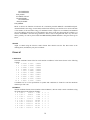
DIVCON
(Lite version)
User Manual
Steven L. Dixon, Arjan van der Vaart,
Bing Wang, Valentin Gogonea, James J. Vincent,
Edward N. Brothers, Dimas Suárez,
Lance M. Westerhoff and Kenneth M. Merz, Jr.*
Department of Chemistry
152 Davey Laboratory
The Pennsylvania State University
University Park
Pennsylvania 16802
Table Of Contents
Introduction
3
Reference Information
4
License Information
4
Help and Website
4
Installation of DivCon Lite
5
Makefile
Compiler Directives
6
6
DivCon Input Format
7
Keywords
8
Hamiltonian
Geometry Optimization
Convergence Criterion
Minimum Optimization
Transition Structure Optimization
Restrained Atoms
Frequency Calculations
Output
General
Gradient
Atomic Charges
Subsetting
8
9
9
9
12
13
13
14
16
20
20
21
Parameters
23
Optimizing DivCon
25
Speed and Memory
Convergence
25
25
References
27
Index of Keywords
29
2
Introduction
DivCon Lite is a linear scaling semiempirical program for calculation of energies, charges and geometries
of systems up to ~20 000 atoms. Available features include:
• linear scaling Divide and Conquer (D&C) calculations[1-3]
• cubic scaling standard calculations[4-6]
• single point AM1,[5] PM3[6] or MNDO[4] calculations
• geometry optimization
• Frozen Density Matrix approximation[7]
• Mulliken,[8] CM1[9] and CM2[10] charge analysis
• Parallel processing using MPI[11]
The program was mainly developed by Steve Dixon. His work includes the development of the
semiempirical Divide and Conquer algorithm, implementation of the D&C and standard energy and
gradient calculations, geometry optimization routines, Mulliken charge analysis, cluster based subsetting
strategy and front end of the program. Arjan van der Vaart added the Monte Carlo routines (single and
multi processing), Particle Mesh Ewald routines, grid based subsetting routines, extension of the cluster
based subsetting schemes, CM1 and CM2 charge analysis, density matrix build routines, density of state
analysis, frozen density matrix routines, the interaction energy decomposition routines (serial and
parallel), and Talman’s algorithm. Bing Wang made this Lite version and put into AMBER to do QM/MM
calculation. Jim Vincent parallellized the single point energy and geometry optimization routines. Ed
Brothers added dipole and ionization potential routines, the parametrization routines and the sodium
parameters. Dimas Suárez added the LBFGS optimization routines, the transition state routines and the
frequency calculation routines.
3
Reference Information
DivCon Lite should be referenced as:
S. L. Dixon, A. van der Vaart, B. Wang, V. Gogonea, J. J. Vincent, E. N. Brothers, D. Suárez, L. M.
Westerhoff and K. M. Merz Jr., DivCon Lite, The Pennsylvania State University, University Park, PA
16802, 2004.
Strongly recommend to see reference [2, 3] for scientific background and implementation details.
Help and Website
Additional information and help can be found at the DivCon website. The address for this website is:
http://merz.chem.psu.edu/divcon/index.html
Questions about DivCon that are not addressed in this manual or on the website can be emailed to:
[email protected]
4
Installation of DivCon Lite in AMBER
edit the divcon.dim file for your system specifications (number of atoms etc.)
% vi divcon.dim
compile by invoking make
% make divcon
the executable will be called divcon and is placed in the current directory
% ls divcon
to run divcon, simply type
% divcon
or, for the parallel divcon version (here using 4 processors)
% mpirun –np 4 divcon
5
Compiler Directives
Compiler directives are used to optimize speed and memory usage of divcon. You can turn off a directive
by commenting the directive-statement (C#define) in the “divcon.dim” file and turn it on by removing the
comment symbol (#define).
MPI_IS_ON
activate this whenever MPI (parallel processing) is used. See page 43 for examples.
MPI_NOMC
activate this whenever MPI is used for single point and geometry optimizations. Inactivate this whenever
MPI is used for Monte Carlo calculations, or whenever MPI is not used.
CUTREPUL_IS_ON
activate this to allow for the CUTREPUL keyword (see page 19). Inactivate this when CUTREPUL is not
used to increase the speed of the calculation.
LARGE_MEMORY_MC
activate this to allow the density matrix to be reset to it's original contents after a rejected step. This will
have a positive (but modest) effect on the computation time, but will increase memory usage quite a bit.
Do not activate when no MC-simulation is performed.
MEMORY_OVERLAP
activate this to allow multiple use of some arrays. This will decrease memory usage without affecting the
accuracy or speed of the calculation.
STEWART_INTEGRALS
activate this to use Stewart’s algorithm[12] for calculation of the overlap matrix. When inactivated,
Talman’s algorithm[13] will be used (with Gs calculated by Hierse and Oppeneer’s algorithm[14]). Both
methods give essentially the same results (differences in heat of formation in 4th decimal) in essentially the
same time (for sp-basis).
6
DivCon Input Format
Schematically the divcon input file (divcon.in) has the following format:
Keywords: 1line minimum, more lines when line is ended at a ‘&’, maximum 80 characters per line.
Title: maximum 80 characters
Atom, Coordinates and Residue information: (see below)
END_COORD: to specify end of coordinates.
Parameters: see page 25.
Here, the parameters contain information about subsetting etc.
The format of atom, coordinate and residue information is:
1
O
4.7092732 3.8021271 8.9033802 RES
2
H
5.0723235 4.3719820 9.5513718
3
H
4.9639974 4.1517696 8.0556286
4
O
0.8528918 0.3470596 0.1015257 RES
5
H
0.1648828 0.9302319 -0.1495947
6
H
1.6391883 0.8006957 0.2127379
which indicates that the first residue is atom 1-3 and the second residue atom 4-6. Coordinates are in Å
and you can use as much white space as you want (maximum characters per line is 80).
Note: do not use tabs in the input file. Use space instead.
Available atoms for MNDO are:
H,[4] Li,[15] Be,[16] B,[17] C,[4] N,[4] O,[4] F,[18] Na (as sparkle),[19] Al,[20] Si,[21] P,[22] S,[23]
Cl,[24] Zn,[25] Ge,[26] Br,[27] Sn,[28] I,[29] Hg,[30] Pb.[31]
Available atoms for AM1 are:
H,[5] Li,[15] Be,[16] B,[32] C,[5] N,[5] O,[5] F,[33] Na,[34] Al,[35] Si,[36] P,[37] S,[38] Cl,[33] Zn,[39]
Ge,[40] Br,[33] I,[33] Hg.[41]
Available atoms for PM3 are:
H,[6] Be,[42] C,[6] N,[6] O,[6] F,[6] Na,[34] Mg,[42] Al,[6] Si,[6] P,[6] S,[6] Cl,[6] Zn,[42] Ga,[42]
Ge,[42] As,[42] Se,[42] Br,[6] Cd,[42] In,[42] Sn,[42] Sb,[42] Te,[42] I,[6] Hg,[42] Tl,[42] Pb,[42]
Bi.[42]
7
Keywords
Hamiltonian
AM1
AM1 Hamiltonian to be used.[5]
PM3
PM3 Hamiltonian to be used.[6]
MNDO
MNDO Hamiltonian to be used.[4]
NOTE: One Hamiltonian must be selected. There is no default.
EXTERNAL=STRING
use parameters from the file with filename indicated by the string (max. 20 characters, filename should be
capitalized). The parameters listed in this file replace the standard AM1/PM3/MNDO parameters. The
format of the external file is:
DATA NAME(...) / ... /
and/or
NAME(...) / .... /
and/or
NAME(...) = ....
e.g.
DATA AL1(0,1) / 0.5345D0/
You can use as much white space as you want, and a capital C (“C”) in the first column is treated as
comment.
NOTNAMED=STRING
when used with the external keyword, the parameters that are not listed in the external file are set to the
standard AM1 parameters when STRING is AM1, to PM3 when STRING is PM3, or to the MNDO values
when STRING is MNDO. Note that these parameters are initialized to zero by default.
PRTPAR
print the AM1/PM3/MNDO parameters for all atom types that occur in the input file
8
Geometry Optimization
DivCon 99 includes various optimization techniques[43] to locate both minima and first-order saddle
points (transition structures). On the one hand, the algorithms for locating minima are specially adapted to
treat large optimization problems. On the other hand, the methods for optimizing transition structures in
DivCon 99 work reasonably well for small and medium size systems.
MAXOPT=INTEGER
do a maximum of INTEGER cycles of optimization. Default: 10 x Number of Geometrical Parameters.
(Note: MAXOPT and OPTMAX are interchangeable)
Convergence Criterion
ETEST=FLOAT
user defined geometry optimization energy change criterion. Default : 0.002 kcal/mol.
GTEST=FLOAT
user defined maximum gradient component criterion. Default : 0.500 kcal/ (mol Å).
XTEST=FLOAT
user defined geometry optimization coordinate change criterion. Default : 0.001 Å / 0.001 degrees.
Minimum Optimization
For the semiempirical minimization of large biomolecules, it is advisable to take the starting point from a
previously Force-Field minimized structure. Note also that there is no default optimization method.
OPT=STEEP
Geometry optimization proceeds by means of function evaluations along the search direction defined as
the minus gradient vector. The steepest descent algorithm is very simple and requires only storage of the
gradient. It is well known that this method can oscillate around the minimum path towards the critical
point and its rate of convergence slows down as the minimum is approached. STEEP should be used
mainly to partially relax a poor starting point during a given number of optimization cycles.
OPT=CONJGRAD
The conjugate gradient method performs quite robust energy minimization along a line that is constructed
so that it is "conjugate" to the previous search directions. This avoids the partial "undoing" on every
optimization step observed in the steepest descent method. The conjugate gradient method avoids
handling of the Hessian and requires only storage for two gradient vectors. Usually, this has been the
method of choice for treating very large systems (hundreds and thousand of atoms) by means of classical
Force Field or Quantum Mechanical Semiempirical methods.
9
OPT=BFGS
A fast pseudo Newton-Raphson algorithm, which expands the Energy function to second order around the
current point using an approximate Hessian, is also implemented in DivCon 99. The BFGS (BroydenFletcher-Goldfarb-Shanno) formula is the most popular Hessian updating scheme to minimize molecular
geometries and ensures the positive definite character of the updated Hessian matrix. However, the
method requires the storage, inversion and updating of the full Hessian matrix. This algorithm is practical
for only medium size systems and the corresponding BFGS routines are dimensioned to manage only a
subset of atoms (see the divcon.dim file in the DivCon 99 distribution for further details).
OPT=LBFGS
The Limited memory BFGS minimizer can be used to minimize large systems efficiently.[44] The LBFGS
method stores only diagonal Hessian and small number m of previous steps and gradient vectors. The
amount of storage can be controlled by the user (m=5 by default, see also the divcon.dim and lbfgs.F files
in the DivCon 99 distribution). This pseudo Newton-Raphson algorithm performs quite well for highly
non-linear functions, requiring about 2 times less function and gradient evaluations than the Conjugate
Gradient method implemented in DivCon 99. This method should be used routinely when optimizing large
systems.
LSEARCH=FLOAT
LSEARCH is a variable with default value of 1.0, which controls the accuracy of the line search routine in
the LBFGS minimizer. Lower values result in a more accurate linear search at the cost of requiring more
energy and gradient evaluations. If the linear search fails during a LBFGS minimization run, changing the
value of LSEARCH may be a remedy of the problem.
NOLNSR
The linear search during a LBFGS minimization is not performed. Pure LBFGS steps are taken by the
minimizer.
DIAGTERM=FLOAT
DIAGTERM is a variable with default value of 0.0001, which scales the initial diagonal form of the
inverse Hessian in the LBFGS minimizer. Low values are recommended when optimizing large systems.
DIIS / NODIIS
The DIIS method attempts to find an optimum linear combination of previous geometries.[45] The
corresponding linear coefficients are determined by minimizing the norm of an interpolated error vector
built as a combination of error vectors. Among the different approaches used to define the DIIS error
vectors, DivCon 99 uses the quasi Newton-Step error vector and the energy error vector for OPT=LBFGS
and OPT=BFGS, respectively. For the LBFGS method, NODIIS is the default option (see below) whereas
DIIS is the default for the standard BFGS algorithm. Note that the DIIS technique needs to store
coordinates and gradients of the last mdiis optimization steps (see the divcon.dim file).
The usual implementation of the DIIS technique for the OPT=BFGS method has been included in DivCon
99 while the DIIS module for the LBFGS method has been especially adapted for treating large systems.
In order to increase the efficiency of the LBFGS-DIIS method, the computation of the error vector takes
advantage of the LBFGS updating scheme of the inverse Hessian matrix and is only activated at the latter
stages of a minimization run. For some systems, the DIIS technique consistently reduces the number of
optimization cycles maintaining a favorable CPU rate with respect to the NODIIS LBFGS method.
However, the DIIS-LBFGS method is more unstable given that sudden increases of the gradient norm may
occur, halting thus the optimization run.
FORCE-IT
Geometry optimization will halt if the energy increases on three successive cycles unless the user
10
overrides it with the keyword FORCE-IT.
11
Transition Structure Optimization
Transition structure (TS) optimizations can be carried out with the Partitioned Rational Function
Optimization, the Newton Raphson or the Quasi Newton Algorithm. All of these are common methods
which are based on some form of augmented Hessian Newton-Raphson approach and use the Powell
update formula. Since these methods require the full Hessian matrix, the corresponding routines, as
implemented in DivCon 99, are dimensioned to manage only a subset of atoms (see the divcon.dim file).
Location of a TS demands a quite accurate Hessian which can be obtained from an updating scheme
(Powell formula is used by DivCon 99) and/or the numerical calculation of the second derivative matrix.
OPT=TS
Use the Partitioned Rational Function optimized (see below, page 14).
OPT=TSNR
The standard Newton Raphson (NR) formula is used to calculate the optimization step within a trust
radius of 0.10 Å. Provided that the initial geometry is close to the TS and the Hessian has exactly one
negative eigenvalue, this method should converge to the correct solution.
OPT=TSPRFO
With respect the NR formula, the augmented Hessian methods are designed to generate a search towards a
saddle point, even when started in a region where the Hessian has not the correct structure. The P-RFO
algorithm employs two shift parameters of the Hessian eigenvalues in order to ensure a proper
maximization along the TS mode and minimization along the rest of modes. The norm of P-RFO step is
scaled down when its value is greater than 0.10 Å. Identical to OPT=TS (see page 14).
OPT=TSQNA
The QNA method (also known as the Trust Radius Image Minimization) uses only one shift parameter
and restricts the total step length to the trust radius whose optimum value is changed along the
optimization.
HESS=CALCFC
Hessian is calculated numerically at the initial point and subsequently updated using the Powell formula
(Default option).
HESS=CALCDUMP
Hessian is calculated numerically at the initial point and every DUMP cycles of optimization (see also the
DUMP keyword).
HESS=CALCALL
Hessian is calculated numerically every optimization step.
HESS=READ
The initial Hessian is read from the HESS parameter in the input file with format READ(INPT,'(5E16.8)')
((HESS(I,J),J=1,I),I=1,3*NATOMS). Default units of the Hessian elements are kcal/(mol Å2).
12
NOMODEFOLLOW
disable the use of the mode following technique. To ensure that the TS mode is being followed smoothly
from one iteration to the next, the P-RFO and QNA algorithms follow the mode which has the greatest
overlap with mode followed on the previous cycle.
Restrained Atoms
BELLY
A subset of the atoms in the system, the belly group, will be allowed to relax their position during
optimization while the rest of the atoms will be kept at fixed positions by zeroing the corresponding
forces. Currently, the BELLY option requires optimization of both minimum or transition structures using
cartesian coordinates (a FREQ calculation can be also subjected to the BELLY option).
The BELLY parameter must be included in the input file in order to specify the BELLY group. Two
formats are possible:
BELLY
ATOMS 144-178 310-332
END_BELLY
This means that the BELLY group of moving atoms will be constituted from atom 144 to atom 178, and
from atom 310 to atom 332. Alternatively, the BELLY group can be selected using residue numbering:
BELLY
RESIDUES 10-13 20
END_BELLY
Only residues from 10 to 13 and residue 20 will be allowed to move during minimization.
Frequency Calculations
FREQ
computes force constants and the resulting vibrational frequencies using double numerical differentiation
with a step size of 0.01 Å. This value of the step size represents a good compromise between accuracy and
numerical problems. The resultant Hessian matrix in cartesian coordinates is written in the divcon.hss
output file with units of kcal/(mol Å2). Vibrational frequencies are computed by determining the second
derivatives of the energy with respect to nuclear coordinates followed by transformation into massweighted coordinates. Of course, this is only valid at a critical point. By specifying both FREQ and OPT
keywords, the frequencies will be computed after successful completion of the optimization task.
13
Output
PRTSUB
print subsystem atom lists.
PRTVEC
print final eigenvectors. All eigenvectors and eigenvalues will be printed by default. If the input file contains
PRTVEC parameters, only some eigenvectors will be printed:
PRTVEC
1-458 all
558-960 -15.0 -10.0
45-460 ef 10.0
END_PRTVEC
The first line indicates that only the eigenvectors for atoms 1-458 need to be printed. These are all
eigenvectors when a standard calculation is performed. For a D&C calculations, these are the eigenstates
for subsystems that contain atoms 1-458. The second line indicates that the eigenstates for atoms 558
through 960 will be printed if the associated eigenvalues are between –15.0 and -10.0 eV. The third line
indicates that the eigenvectors of atoms 45-460 will be printed if the associated eigenvalues are within 10
eV of the Fermi energy.
DOS
perform a density of state analysis. By default, a DOS analysis will be performed on all eigenvalues for all
atoms, with interval of 0.5 eV. Intervals and extend of the DOS analysis can be set by the DOS
parameters:
DOS
1-435 0.2
1015-4452 0.3
END_DOS
Here the DOS will be printed for all subsystems that contain atoms 1-435 with interval of 0.2 eV and for
all subsystems that contain atoms 1015 through 4452 with interval of 0.3 eV. Note that for a standard
calculation the DOS will always extend over all atoms.
DIPOLE
calculate the magnitude of themolecular dipole moment using all three charge methods.
IP
calculate ionization potential
HOMOLUMO
calculate homo-lumo gap. For a D&C run, the homo-lumo gap of all subsystems will be printed.
PRTCOORDS
print atomic coordinates .
PRTPAR
14
print the AM1/PM3/MNDO parameters for all atom types that occur in the input file
SCREEN
output vital information to screen.
WRTPDB
write final coordinates in pdb format.
DUMP=INT
write restart file (divcon.rst) every INT cycles.
PDUMP=INT
write density matrix file (divcon.dmx) every INT SCF iteration
SNAPGEOM
write coordinates during energy optimization (divcon_snapshot.N) at every N-th optimization step. This
can be useful when optimizing very large systems.
TRAJECTORY
dump coordinates to trajectory file (divcon.trj) at restart points.
CALCGEO
Calculates geometric parameters. Input takes the form (after the END_COORD line):
GEO
DISTANCE
1-2
END_DISTANCE
ANGLE
1-2-3
END_ANGLE
DIHEDRAL
1-2-4-3
END_DIHEDRAL
END_GEO
Note that if an equals sign is included after the atom numbers (i.e. 1-2=2.0) then a set of differences
between the calculated values and these numbers are returned.
ERROR
Calculates the difference between accepted and calculated values. An example list is shown below, with
each component being explained afterward. Note this is only usable with standard calculations, and this
list follows the END_COORDS line.
ERROR
HEAT=FLOAT
IP=FLOAT
DIPOLE=FLOAT
ASSOCIATION=FLOAT
15
FILExINTEGER
FILExINTEGER
END_ASSOC
ETOTDIFF=FLOAT
FILExINTEGER
FILExINTEGER
END_ETOTDIFF
END_ERROR
HEAT is the heat of formation in kcal/mol. IP is ionization potential. DIPOLE is the Mulliken dipole.
ASSOCIATION is the energy of association, and the lines following it are the files to be used to calculate
it. For instance, if the association energy of a methanol-2 water complex was to calculated, and methanol
was in divcon001.in and water was in divcon002.in, the values on the two subsequent line would be 1x1
and 2x2. ETOTDIFF is the total energy difference, and it’s files are designated the same way. Note also
that a geometry list can be placed inside the ERROR/END_ERROR delimiters using the format given
above.
ZMAKE
output a z-matrix using the DivCon z-matrix format. Note that this uses the first three atoms as the
defining atoms, and thus they may not be collinear.
General
CARTESIAN
Cartesian coordinate format. DivCon reads cartesian coordinates in the format shown in the following
example:
1
N
-0.26120
-0.98976
0.00000
2
C
0.64694
0.01940
0.00000
3
C
-0.47100
1.06738
0.00000
4
C
-1.44202
-0.13945
0.00000
5
O
1.83331
0.04003
0.00000
6
H
-0.13870
-1.97802
0.00000
7
H
-0.49385
1.68899
-0.88436
8
H
-0.49385
1.68899
0.88436
9
H
-2.05887
-0.23715
-0.88402
10
H
-2.05887
-0.23715
0.88402
Coordinates are in Å. The specification of symbols and coordinates is format free and the maximum
characters per line is 80.
INTERNAL
internal coordinate format selected (similar to that of MOPAC). DivCon reads z-matrix coordinates using
the format shown in the following example:
1
N
0.000 0
0.000 0
0.000
0
0
0
2
C
1.357 1
0.000 0
0.000
1
0
0
3
C
1.532 1
91.166 1
0.000
2
1
0
4
C
1.455 1
96.226 1
0.000
1
2
3
5
O
1.186 1
132.979 1
180.000
2
1
3
6
H
0.995 1
130.950 1
179.987
1
2
3
7
H
1.081 1
114.061 1
243.684
3
2
1
8
H
1.081 1
114.061 1
116.319
3
2
1
9
H
1.083 1
114.126 1
116.416
4
1
2
16
10
H
1.083 1
114.126 1
243.596
4
1
2
The first column contains the atom numbering followed by the corresponding atomic symbol. For each
atom in the z-matrix, bond distance, bond angle and dihedral angle are specified as real numbers followed
by their optimization integer flags (0=fixed variable, 1=free variable). The last three columns specify the
z-matrix connectivity in terms of the corresponding atom numberings. Bond distances are in Å while bond
angles and dihedral angles are in degrees. The specification of the z-matrix parameters is format free and
the maximum number of character per line is 80.
NOTE: Either Cartesian or internal coordinates must be specified.
RMIN=FLOAT
The minimum allowed distance between atoms (results in an error for single point calculations and
geometry optimizations, configuration will be rejected in an MC-run when a smaller distance is
encountered).
ECRIT=FLOAT
set the convergence for the energy in units of eV. (default value is 4·10-6 eV). ECRIT is identical to the
DESCF keyword.
DCRIT=FLOAT
set the convergence for the density matrix in atomic units (default value 5·10-4 e). DCRIT is identical to
the DPSCF keyword.
CUTREPUL=FLOAT
only active when CUTREPUL_IS_ON is defined in divcon.dim. Set the [xy|xy], [xz|xz], [xx|yy], [xx|zz],
[zz|xx], [xx|xx] and [zz|zz] integrals to zero when the interatomic distance is larger than FLOAT.
CUTBOND=FLOAT
cutoff bonding for the H, P and F matrixes beyond FLOAT angstroms.
DESCF=FLOAT
user defined SCF energy criterion (identical to ECRIT keyword).
DPSCF=FLOAT
user defined SCF density matrix criterion (identical to DCRIT keyword).
DIRECT
do not store 2-electron integrals in SCF calculations.
FULLSCF
do full diagonalizations in SCF calculation (no pseudo diagonalizations).
ADDMM
17
add MM correction to peptide torsional barrier.
NOMM
do not use molecular mechanics correction for peptide torsions.
RESIDUE
store residue pointers. Needed for D&C calculations.
CHKRES
check inter-atomic distances for each residue.
TEMPK=FLOAT
user defined divide and conquer temperature. Units are Kelvin, and default is 1000K.
TESTRUN
do setup work and stop before first energy evaluation.
TMAX=FLOAT
user defined maximum CPU time in seconds.
ROTATE=FLOAT
set the rotation angle for energy barrier
GEOM=PDB
input is in PDB format
PBC
periodic boundary conditions in effect. This only works when a box is specified through the BOX
parameters:
BOX
XBOX=20.0 YBOX=20.0 ZBOX=20.0
END_BOX
which means that the box dimensions are 202020 Å.
Note that for a single point calculation / geometry optimization where RESGRID was not specified all
atoms should be contained within the box, for all other cases all center of masses of the residues should be
within the box.
RESTART
read in restart file from previous run. To create the restart file, please see dump (page 17).
SHIFT=FLOAT
18
user defined initial dynamic level shift[46] parameter in eV.
XYZSPACE
do all operations in xyz space.
MAXIT=INT
Set the maximum number of SCF iterations (default: 1000)
1SCF
Perform only the first SCF iteration, i.e. calculate the energy through E = 0.5(H+F)P. Note that this is not
equivalent to MAXIT=1, since no diagonalization is performed.
GUESS
Build the initial density matrix from one or more density matrix files. These files are listed by means of
the GUESS parameters:
GUESS
A.dmx
b.dmx
END_GUESS
Build the initial density matrix from the files A.dmx and b.dmx. The density matrix elements of atoms 1
through a are read from A.dmx, for atoms a+1 through n from file b.dmx.
GUESS
2-10 A.dmx 33-41 f
20-30 b.dmx 1-11
END_GUESS
Density matrix information for atoms 2-10 is read from the density matrix elements of atoms 33-41 of file
A.dmx, density matrix information for atoms 20-30 is read from the density matrix elements of atoms 111 from file b.dmx. Missing density matrix elements are auto-initialized and a correction will be applied
to constrain the total number of electrons. The density matrix elements of atoms 2-10 will be kept constant
during the SCF iterations by using the Frozen Density Matrix approximation.[7] It is imperative that the
number of orbitals on a certain atom in the divcon.in file and density matrix file are the same, i.e. the
number of orbitals on atom 2 from divcon.in and atom 33 from A.dmx should be identical.
Note that the maximum length of a density matrix file name is 20 characters, no dashes (“-“) are allowed
in the density matrix file name.
FILES
Performs calculations for a set of molecules contained in files named divcon001.in, divcon002.in etc.
These files can have the same keywords as the divcon.in file, with the exception that they are restricted to
standard calculations (no D&C) and they may not be solvation calculations (no SCRF).
PUSH
Only in combination with the CLUSTER keyword (page 23) and when multiple cores (i.e. multiple cluster
groups) are defined. Push the different cluster groups apart. Default is 106 Å, the user can define this
distance by using PUSH=FLOAT. When more than two cluster groups are defined, each group is place on
a gridpoint with gridspacing of 106 Å or the user defined value.
19
Gradient
GRADIENT
output final gradient.
CENTRAL
use central difference in gradient calculation.
INTER
include only intermolecular contributions for gradient calculation (skip intramolecular contributions). This
is default for MC-simulations.
Atomic Charges
CHARGE=INT
a net charge is to be placed on system.
MULLIKEN
use Mulliken[8] charges for PME and/or SCRF, write Mulliken charges to charge output file of MC-run.
CM1
use CM1[9] charges for PME and/or SCRF, write CM1 charges to charge output file of MC-run.
CM2
use CM2[10] charges for PME and/or SCRF, write CM2 charges to charge output file of MC-run.
NOTE: For a single point calculation and geometry optimization both Mulliken, CM1 and CM2 charges
are calculated, for a MC-run only the one specified.
Subsetting
This is the basis of divide and conquer methodology.[1-3] Subsetting can be performed by hand through
the SUB parameters (page 31), or automatically through the keywords listed below. Subsystems consists
of a core surrounded by an inner and outer buffer.[3]
CLUSTER
do cluster based subsetting. Specification of the cluster based subsetting is through the cluster parameters:
CLUSTER
NCORE=3 DBUFF1=4.0 DBUFF2=2.0
20
END_CLUSTER
This means that the cores will be build from 3 residues, the first buffer region extends 4.0 Å from the core,
the second buffer region 2.0 Å from the first buffer region. Multiple cores (i.e. multiple cluster groups)
can be defined by:
CLUSTER
NCORE=2 (1-6 7 8 12-14)
NCORE=3 (9 10 15-25 )
NCORE=1 (26 27)
DBUFF1=4.3 DBUFF2=2.0
END_CLUSTER
Cores will be build from 2 residues for residues 1-6, 7, 8, 12-14, from 3 residues for residues 9, 10, 15-25
and from 1 core for residue 26 and 27. The first buffer region is 4.3 Å, the second 2.0 Å. Note that all
residues should be used (and only once) in this syntax.
CLUSTER
NCORE=1 (1-20) [-1]
NCORE=1 (21-100) [0]
END_CLUSTER
Cores will be build from 1 residue for residues 1-20 and from 1 residue for residues 21-100. Moreover, the
charge of the subsystems build from residues 1-20 will be contrained to –1 electron and the charge of the
subsystems build from residues 21-100 to 0 electrons. Only effective when the NO-OVERLAP keyword is
used (see page 24). Charges are constrained by use of multiple Fermi energies.[47]
NO-OVERLAP
Only in combination with the CLUSTER keyword.
CLUSTER
NCORE=1 (1-10)
NCORE=1 (11-20)
END_CLUSTER
When the NO-OVERLAP keyword is used, subsystems made from residues 1-10 only overlap with
subsystems made from residues 1-10 and subsystems made from residues 11-20 only overlap with
subsystems made from residues 11-20. In other words, density matrix elements between subsystems 1-10
and 11-20 are zero.
ATGRID
do grid based, atom-wise subsetting (core and buffers will be build from atoms).
RESGRID
do grid based, residue-wise subsetting (core and buffers will be build from residues).
MIXGRID
do grid based, residue-wise subsetting for cores, grid based, atom-wise subsetting for buffers.
NOTE: Specify Grid parameters when a grid based subsetting is selected. The syntax for these parameters
is:
GRID
XCORE=4.0 YCORE=4.0 ZCORE=4.0 OVERLAP=0.5
DBUFF1=2.5 DBUFF2=1.0
END_GRID
Meaning that the total system will be divided into rectangular boxes of 4.04.04.0 Å that overlap 0.5 Å in
each dimension. The first buffer region is 2.5 Å wide, the second 1.0 Å.
NOTE: In Monte Carlo simulations only a residue-wise grid-based subsetting scheme is allowed. Reason
21
for this is rather subtle: Imagine that during the MC-simulation a molecule would penetrate the box, such
that the geometric center is still inside the box, but some atoms are outside the box. If an atom based
subsetting was performed, the atoms outside the box wouldn't be included in any subsystem. Making the
"grid-subsetting"-box artificially larger than the pbc-box wouldn't work either: in that case there's is an
artificially larger distance between the molecules and the (virtual, pbc) images of other molecules. This
would mean that some atoms will be skipped in making the buffer regions: atoms that, according to their
pbc-image should be included. This will lead to non-optimal subsettings and can have a rather drastic
effect on energies as was found experimentally.
COMBSUB
do a combination subsetting; certain residues will be subsetted grid based, others cluster based. Use the
combsub parameters to specify this subsetting:
COMBSUB
CLUSTER
1-10 13
RESGRID
11-12 14-20
END_COMBSUB
Here, cluster based subsetting will be done for residues 1-10 and 13, gridbased residue-wise subsetting
will be done for residues 11-12 and 14-20. The cores of the subsystems will be selected from the specified
residues, buffers from all residues / atoms of the system. COMBSUB can only be defined as a
combination of CLUSTER with one of RESGRID, ATGRID of MIXGRID. Note that you have to specify
the CLUSTER and GRID parameters when you use COMBSUB. Note that all residues should be used
(and only once) in COMBSUB.
STANDARD
standard closed-shell calculation (no divide and conquer). All subsetting parameters are ignored, only one
subsystem containing all atoms will be generated.
22
Parameters
SUB
Reads in atom list for handwise subsetting.
SUB
SUB 1
CORE
123
BUFFER_1
789
BUFFER_2
4 5 6 10
END_SUB
There is one subsystem, the core is build from atoms 1, 2 and 3, the first buffer from atoms 7, 8 and 9, the
second buffer from atoms 4, 5, 6, 10. Note that all residues should be named at least once in the cores.
BOX
Reads in the box dimensions for a PBC calculation. See page 21.
BELLY
Reads in belly parameters for geometry optimization. See page 15.
CLUSTER
Reads the parameters for the cluster based subsetting. See page 23.
GRID
Parameters for gridbased subsetting. See page 23.
COMBSUB
Parameters for combination subsetting. See page 24.
DOS
Parameters for density of state analysis. See page 16.
PRTVEC
Parameters for eigenstate analysis. See page 16.
GUESS
23
Parameters for density matrix build. See page 21.
NEIGHBORS
Only in combination with CLUSTER subsetting (used with the multiple core and Fermi feature, see page
23) and NO-OVERLAP keyword (page 24)
NEIGHBORS
NEIGHBORS=2 1
NEIGHBORS=1 3
END_NEIGHBORS
Specifies the overlap of residues in the first and third cluster groups. Residues in the first cluster group
only overlap with residues of the first cluster group if they are within 2 residues away from each other.
Residues in the third cluster group only overlap with residues of the third cluster group if they are within 1
residue away from each other. For example:
CLUSTER
NCORE=1 (1-10) [0]
NCORE=1 (11-20) [0]
NCORE=1 (21-30) [0]
DBUFF1=4.0 DBUFF2=2.0
END_CLUSTER
NEIGHBORS
NEIGHBORS=2 1
NEIGHBORS=1 3
END_NEIGHBORS
Here atoms of residue 1 (which is in the first cluster group) will only overlap with atoms of residue 1, 2
and 3 (that is, if they are within the buffer region). Atoms of residue 5 will only overlap with atoms of
residue 3, 4, 5, 6 and 7 and atoms of residue 30 only with atoms of residues 29 and 30.
24
Optimizing DivCon
Speed and Memory
For high performance, edit the divcon.dim file to the right dimensions for your system. Settings that are
too small will cause DivCon to exit, settings that are too large significantly increase memory use and
computation time. Use the compiler directives to tailor DivCon to your needs (page 7). Do not uncomment
the SCRF capabilities in the Makefile if you don’t need them (page 7): uncommenting the SCRF lines
results in an executable about 4 times slower (due to smart memory algorithms in DelPhi). Use the
MEMORY_OVERLAP directive (page 7) to decrease memory use and speed up the calculations.
For large systems, use the CUTBOND option to decrease memory use (page 19). A value larger or equal
to 8 usually gives good accuracy. Use the DIRECT keyword to avoid storage of the integrals (page 20).
DIRECT increases the computation time by ≤ 15%, but severely decreases memory usage.
Convergence
Convergence can be sped up by constructing the initial density matrix from guess density matrices (page
21). Speedup is only significant when large portions are captured in the guess density matrices and when
geometries are very similar. For large systems and highly charged systems, convergence can be sped up
by use of multiple Fermi energies. For example, in a protein-water system, first perform a calculation of
the water system without protein and the protein without water. Use these two density matrices as guess
for the next calculation, but only allow polarization: use the NO-OVERLAP keyword (page 24) and
constrain the charge of protein and water to their formal charges by using multiple Fermi energies (page
23 and 33). Then, completely relax the system by using only one Fermi energy and by allowing all
subsystems to overlap, using the previously generated density matrix file as guess (see also page 37). If
these tricks don’t work, polarize the solvent and solute separately (see page 41).
Use increasingly larger buffer regions for systems that are very hard to converge, using the density matrix
of the previous calculation as guess. Increasing the CUTBOND (page 19) in steps also speeds up
convergence. Computation time can be decreased by using loose convergence criteria for low quality
subsetting (i.e. subsetting with small buffers and small CUTBOND values) and tightening these criteria
for higher quality subsetting (see page 11).
Use of the SHIFT keyword (page 21) also speeds up convergence. Suggested values are 2.5 or 5.0.
As example, we will show here the convergence of a highly charged solvated species. Note that the
number of steps and tricks is very dependent on the system of interest: your system may require more or
less steps.
A) converge the solute at low quality (lowsolute.in)
... DIRECT CUTBOND=7.0 ECRIT=1.0E-3 DCRIT=1.0E-2 SHIFT=5.0 CHARGE=10
...
CLUSTER
NCORE=1 DBUFF1=3.0 DBUFF2=2.0
END_CLUSTER
B) converge the solute at high quality (highsolute.in)
25
... DIRECT CUTBOND=8.0 CHARGE=10 GUESS
...
CLUSTER
NCORE=1 DBUFF1=4.5 DBUFF2=2.0
END_CLUSTER
GUESS
lowsolute.dmx
END_GUESS
C) converge the solvent (solvent.in)
... DIRECT CUTBOND=8.0 CHARGE=0
...
CLUSTER
NCORE=1 DBUFF1=4.5 DBUFF2=2.0
END_CLUSTER
D) solvate the system, first polarize the solvent (polsolv.in)
... DIRECT CUTBOND=8.0 NO-OVERLAP GUESS CHARGE=10
...
CLUSTER
NCORE=1 (1-100) [10] F
NCORE=1 (101-1000) [0]
DBUFF1=4.5
DBUFF2=2.0
END_CLUSTER
GUESS
highsolute.dmx
solvent.dmx
END_GUESS
E) now polarize the solute (polsolute.in):
... DIRECT CUTBOND=8.0 NO-OVERLAP GUESS CHARGE=10
...
CLUSTER
NCORE=1 (1-100) [10]
NCORE=1 (101-1000) [0] F
DBUFF1=4.5
DBUFF2=2.0
END_CLUSTER
GUESS
polsolv.dmx
END_GUESS
F) converge the whole system
... DIRECT CUTBOND=8.0 GUESS CHARGE=10
...
CLUSTER
NCORE=1 DBUFF1=4.5 DBUFF2=2.0
END_CLUSTER
GUESS
polsolute.dmx
END_GUESS
26
References
1.
2.
3.
4.
5.
6.
7.
8.
9.
10.
11.
12.
13.
14.
15.
16.
17.
18.
19.
20.
21.
22.
Yang, W. and T.-S. Lee, A Density-Matrix Divide-and-Conquer Approach for
Electronic Structure Calculations of Large Molecules. J. Chem. Phys., 1995.
103(13): p. 5674-5678.
Dixon, S.L. and K.M. Merz, Jr., Semiempirical Molecular Orbital Calculations with
Linear System Size Scaling. J. Chem. Phys., 1996. 104: p. 6643-6649.
Dixon, S.L. and K.M. Merz, Jr., Fast, Accurate Semiempirical Molecular Orbital
Calculations for Macromolecules. J. Chem. Phys., 1997. 107(3): p. 879-893.
Dewar, M.J.S. and W. Thiel, Ground States of Molecules. 38. The MNDO Method,
Approximations and Parameters. J. Am. Chem. Soc., 1977. 99(15): p. 4899-4907.
Dewar, M.J.S., et al., AM1: A New General Purpose Quantum Mechanical
Molecular Model. J. Am. Chem. Soc., 1985. 107(13): p. 3902-3909.
Stewart, J.J.P., Optimization of Parameters for Semiempirical Methods I. Method. J.
Comp. Chem., 1989. 10(2): p. 209-220.
Ermolaeva, M.D., A. van der Vaart, and K.M.J. Merz, Implementation and Testing
of a Frozen Density Matrix - Divide and Conquer Algorithm. J. Phys. Chem., 1999.
103: p. 1868-1875.
Mulliken, R.S., Electronic Populations Analysis on LCAO-MO Molecular Wave
Functions. J. Chem. Phys., 1955. 23: p. 1833-1840.
Storer, J.W., et al., Class IV Charge Models: A New Semiempirical Approach in
Quantum Chemistry. J. Comput.-Aided Mol. Design, 1995. 9: p. 87-110.
Li, J., C.J. Cramer, and D.G. Truhlar, New Class IV Charge Model for Extracting
Accurate Partial Charges from Wave Functions. J. Phys. Chem. A., 1998. 102: p.
1820-1831.
Vincent, J.J. and K.M. Merz, Jr., Parallel Implementation of the Divide and
Conquer Algorithm. Theor. Chem. Acc., 1998. 99: p. 220-223.
Stewart, J.J.P., MOPAC: A Semiempirical Molecular Orbital Program. J. Comp.Aided Mol. Design, 1990. 4(1): p. 1-105.
Talman, J.D., Expression for Overlap Integrals of Slater Orbitals. Phys. Rev. A,
1993. 48(1): p. 243-249.
Hierse, W. and P.M. Oppeneer, Fast and Stable Algorithm for the Analytical
Computation of Two-Center Coulomb and Overlap Integrals over Slater-Type
Orbitals. Int. J. Quantum Chem., 1994. 52: p. 1249-1265.
Thiel, W., MNDOC. 1982, Quant. Chem. Prog. Exch. No. 438.
Dewar, M.J.S. and H.S. Rzepa, J. Am. Chem. Soc., 1978. 100: p. 777.
Dewar, M.J.S. and M.L. McKee, J. Am. Chem. Soc., 1977. 99: p. 5231.
Dewar, M.J.S. and H.S. Rzepa, J. Am. Chem. Soc., 1978. 100: p. 58.
Stewart, J.J.P., Mopac 6.0, QCPE.
Davis, L.P., et al., J. Comp. Chem., 1981. 2: p. 433.
Dewar, M.J.S., et al., Organometallics, 1986. 5: p. 375.
Dewar, M.J.S., M.L. McKee, and H.S. Rzepa, J. Am. Chem. Soc., 1978. 100: p.
3607.
27
23.
24.
25.
26.
27.
28.
29.
30.
31.
32.
33.
34.
35.
36.
37.
38.
39.
40.
41.
42.
43.
44.
45.
46.
47.
Dewar, M.J.S. and C.H. Reynolds, J. Comp. Chem., 1986. 7: p. 140.
Dewar, M.J.S. and H.S. Rzepa, J. Comp. Chem., 1983. 4: p. 158.
Dewar, M.J.S. and K.M.J. Merz, MNDO Calculations for Compounds Containing
Zinc. Organometallics, 1986. 5(7): p. 1494-1496.
Dewar, M.J.S., G.L. Grady, and E.F. Healy, Organometallics, 1987. 6: p. 186.
Dewar, M.J.S. and E.F. Healy, J. Comp. Chem., 1983. 4: p. 542.
Dewar, M.J.S., G.L. Grady, and J.J.P. Stewart, J. Am. Chem. Soc., 1984. 106: p.
6771.
Dewar, M.J.S., E.F. Healy, and J.J.P. Stewart, J. Comp. Chem., 1984. 5: p. 358.
Dewar, M.J.S., et al., Organometallics, 1985. 4: p. 1964.
Dewar, M.J.S., et al., Organometallics, 1985. 4: p. 1973.
Dewar, M.J.S., C. Jie, and E.G. Zoebisch, Organometallics, 1988. 7: p. 513-521.
Dewar, M.J.S. and E.G. Zoebisch, Extension of AM1 to the Halogens. J. Mol.
Struct. (Theochem.), 1988. 180: p. 1-21.
Brothers, E.N. and K.M. Merz, Jr, Sodium Parameters for AM1 and PM3 Optimized
Using a Modified Genetic Algorithm. to be published.
Dewar, M.J.S. and A.J. Holder, Organometallics, 1990. 9: p. 508.
Dewar, M.J.S. and C. Jie, Organometallics, 1987. 6: p. 1486-1490.
Dewar, M.J.S. and C. Jie, J. Mol. Struct. (Theochem), 1989. 187: p. 1.
Dewar, M.J.S. and Y.C. Yuan, Inorg. Chem., 1990. 29: p. 3881-3890.
Dewar, M.J.S. and K.M.J. Merz, AM1 Parameters for Zinc. Organometallics, 1988.
7(2): p. 522-524.
Dewar, M.J.S. and C. Jie, Organometallics, 1989. 8: p. 1544.
Dewar, M.J.S. and C. Jie, Organometallics, 1989. 8: p. 1547.
Stewart, J.J.P., Optimization of Parameters for Semiempirical Methods. III
Extension of PM3 to Be, Mg, Zn, Ga, Ge, As, Se, Cd, In, Sn, Sb, Te, Hg, Tl, Pb and
Bi. J. Comp. Chem., 1991. 12(3): p. 320-341.
Jensen, F., An Introduction to Computational Chemistry. 1999, New York, NY:
John Wiley & Sons.
Baysal, C., H. Meirovitch, and M. Navon, Performance of Efficient Minimization
Algorithms as Applied to Models of Peptides and Proteins. J. Comput. Chem., 1999.
20: p. 354-364.
Eckert, F., P. Pulay, and H.J. Werner, J. Comput. Chem., 1997. 18: p. 1473-1483.
Mitin, A.V., The Dynamic Level Shift Method for Improving the Convergence of the
SCF Procedure. J. Comp. Chem., 1988. 9: p. 107-110.
van der Vaart, A. and K.M. Merz, Jr., Divide and Conquer Interaction Energy
Decomposition. J. Phys. Chem. A, 1999. 103: p. 3321-3329.
28
Index of Keywords
1SCF, 20
ADDMM, 19
AM1, 8
ATGRID, 22
BELLY, 13
CARTESIAN, 16
CENTRAL, 20
CHARGE, 21
CHKRES, 18
CLUSTER, 21, 23
CM1, 20
CM2, 20
COMBSUB, 22, 23
CUTBOND, 17
CUTREPUL, 17
CUTREPUL_IS_ON, 6
DCRIT, 17
DESCF, 17
DIAGTERM, 11
DIIS, 11
DIPOLE, 14
DIRECT, 17
DOS, 14
DPSCF, 18
DUMP, 15
ECRIT, 17
ERROR, 15
ETEST, 9
EXTERNAL, 9
FILES, 19
FORCE-IT, 12
FREQ, 13
FULLSCF, 18
GEOM, 18
GRADIENT, 20
GRID, 23
GTEST, 9
GUESS, 19, 24
HESS=CALCALL, 12
HESS=CALCDUMP, 12
HESS=CALCFC, 12
HESS=READ, 13
HOMOLUMO, 14
29
INTER, 20
INTERNAL, 16
IP, 14
LARGE_MEMORY_MC, 6
LSEARCH, 11
MAXIT, 19
MAXOPT, 10
MEMORY_OVERLAP, 6
MIXGRID, 22
MNDO, 8
MPI_IS_ON, 6
MPI_NOMC, 6
MULLIKEN, 20
NODIIS, 11
NOLNSR, 11
NOMM, 18
NOMODEFOLLOW, 13
NO-OVERLAP, 21
NOTNAMED, 9
OPT=BFGS, 10
OPT=CONJGRAD, 9
OPT=LBFGS, 10
OPT=STEEP, 9
OPT=TS, 12
OPT=TSNR, 12
OPT=TSPRFO, 12
OPT=TSQNA, 12
PARAM_IS_ON, 6
PBC, 19
PDUMP, 15
PM3, 8
PRTCOORDS, 14
PRTPAR, 8, 15
PRTSUB, 14
PRTVEC, 14
PUSH, 20
RESGRID, 22
RESIDUE, 18
RESTART, 19
RMIN, 17
ROTATE, 18
SCREEN, 15
SCRF_IS_ON, 6
SHIFT, 19
SNAPGEOM, 16
STANDARD, 22
STEWART_INTEGRALS, 6
SUB, 29
30
TEMPK, 18
TESTRUN, 18
TMAX, 18
TRAJECTORY, 15
WRTPDB, 15
XTEST, 9
XYZSPACE, 19
ZMAKE, 16
31