Download RealPaver User's Manual

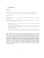
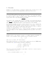
RealPaver User’s Manual
Solving Nonlinear Constraints by Interval Computations
Edition 0.4, for RealPaver Version 0.4
August 2004
Laurent Granvilliers
c 1999–2003 Institut de Recherche en Informatique de Nantes, France.
Copyright c 2004 Laboratoire d’Informatique de Nantes Atlantique, France.
Copyright Laurent Granvilliers
Laboratoire d’Informatique de Nantes Atlantique
Universit´e de Nantes
B.P. 92208, F-44322 Nantes cedex 3, France
[email protected]
The authors hereby grant you non-exclusive and non-transferable license to use, copy and modify
this manual for non-commercial purposes.
Acknowledgements
I would like to thank Fr´ed´eric Benhamou and Fr´ed´eric Goualard for many interesting discussions
on interval constraint satisfaction techniques, and Luc Jaulin who gave me interesting feedback
on an early version of RealPaver.
I am grateful to the members of the Constraint Programming Group at the University of Nantes
for their encouragement. Many thanks to Martine Ceberio who was an incorruptible beta tester.
i
Contents
1 Distribution
License . . . . . . . . . . . . . . . . . . . . . . . . . . . . . . . . . . . . . . . . . . . .
1
1
2 Installation
Software and Hardware Requirements
Installation . . . . . . . . . . . . . . .
Use of RealPaver . . . . . . . . . . . .
Bug Report . . . . . . . . . . . . . . .
.
.
.
.
.
.
.
.
.
.
.
.
.
.
.
.
.
.
.
.
.
.
.
.
.
.
.
.
.
.
.
.
.
.
.
.
.
.
.
.
.
.
.
.
.
.
.
.
.
.
.
.
.
.
.
.
.
.
.
.
.
.
.
.
.
.
.
.
.
.
.
.
.
.
.
.
.
.
.
.
.
.
.
.
.
.
.
.
3
3
3
3
3
3 Overview
Constraint Programming . . . . . . . . . . .
Numerical Constraints . . . . . . . . . . . .
3.1 Modeling with Constraints . . . . . . . . . .
Example: Intersection of Circles . . . . . . .
Constants . . . . . . . . . . . . . . . . . . .
Variables and Domains . . . . . . . . . . . .
Example: Disjunctive Constraints . . . . . .
Grammar of Constraints . . . . . . . . . . .
3.2 Branch-and-Prune Algorithms . . . . . . . .
Example: Intersection of Circles . . . . . . .
Paving or Not . . . . . . . . . . . . . . . . .
Programming the Search . . . . . . . . . . .
Example: Brown’s problem . . . . . . . . .
3.3 Output of RealPaver . . . . . . . . . . . . .
3.4 Consistency Techniques . . . . . . . . . . .
Example: Circle . . . . . . . . . . . . . . .
Strong Consistency Techniques . . . . . . .
Interval Newton . . . . . . . . . . . . . . . .
Programming with Consistency Techniques
3.5 Programming the Strategy . . . . . . . . . .
3.6 Related Work . . . . . . . . . . . . . . . . .
.
.
.
.
.
.
.
.
.
.
.
.
.
.
.
.
.
.
.
.
.
.
.
.
.
.
.
.
.
.
.
.
.
.
.
.
.
.
.
.
.
.
.
.
.
.
.
.
.
.
.
.
.
.
.
.
.
.
.
.
.
.
.
.
.
.
.
.
.
.
.
.
.
.
.
.
.
.
.
.
.
.
.
.
.
.
.
.
.
.
.
.
.
.
.
.
.
.
.
.
.
.
.
.
.
.
.
.
.
.
.
.
.
.
.
.
.
.
.
.
.
.
.
.
.
.
.
.
.
.
.
.
.
.
.
.
.
.
.
.
.
.
.
.
.
.
.
.
.
.
.
.
.
.
.
.
.
.
.
.
.
.
.
.
.
.
.
.
.
.
.
.
.
.
.
.
.
.
.
.
.
.
.
.
.
.
.
.
.
.
.
.
.
.
.
.
.
.
.
.
.
.
.
.
.
.
.
.
.
.
.
.
.
.
.
.
.
.
.
.
.
.
.
.
.
.
.
.
.
.
.
.
.
.
.
.
.
.
.
.
.
.
.
.
.
.
.
.
.
.
.
.
.
.
.
.
.
.
.
.
.
.
.
.
.
.
.
.
.
.
.
.
.
.
.
.
.
.
.
.
.
.
.
.
.
.
.
.
.
.
.
.
.
.
.
.
.
.
.
.
.
.
.
.
.
.
.
.
.
.
.
.
.
.
.
.
.
.
.
.
.
.
.
.
.
.
.
.
.
.
.
.
.
.
.
.
.
.
.
.
.
.
.
.
.
.
.
.
.
.
.
.
.
.
.
.
.
.
.
.
.
.
.
.
.
.
.
.
.
.
.
.
.
.
.
.
.
.
.
.
.
.
.
.
.
.
.
.
.
.
.
.
.
.
.
.
.
.
.
.
.
.
.
.
.
.
.
.
.
.
.
.
.
.
.
.
.
.
.
.
.
.
.
.
.
.
.
.
.
.
.
.
.
.
.
.
.
.
.
.
.
5
5
5
6
6
8
9
10
11
11
11
12
13
14
16
17
17
19
21
23
23
26
.
.
.
.
.
.
.
.
.
.
.
.
.
.
.
.
.
.
.
.
Index
27
References
29
Grammar of the Language
31
iii
1
Distribution
RealPaver 0.4
BSD License
Copyright (c) 1999-2003, Institut de Recherche en Informatique de Nantes (IRIN), France
Copyright (c) 2004, Laboratoire d’Informatique de Nantes Atlantique (LINA), France
All rights reserved.
The following terms apply to all files associated with this software that are mentionned in the
file manifest.txt.
Redistribution and use in source and binary forms, with or without modification, are permitted
provided that the following conditions are met:
• Redistributions of source code must retain the above copyright notice, this list of conditions
and the following disclaimer.
• Redistributions in binary form must reproduce the above copyright notice, this list of conditions and the following disclaimer in the documentation and/or other materials provided
with the distribution.
• Neither the name of the LINA nor the names of its contributors may be used to endorse
or promote products derived from this software without specific prior written permission.
THIS SOFTWARE IS PROVIDED BY THE COPYRIGHT HOLDERS AND CONTRIBUTORS ”AS IS” AND ANY EXPRESS OR IMPLIED WARRANTIES, INCLUDING, BUT
NOT LIMITED TO, THE IMPLIED WARRANTIES OF MERCHANTABILITY AND FITNESS FOR A PARTICULAR PURPOSE ARE DISCLAIMED. IN NO EVENT SHALL THE
COPYRIGHT OWNER OR CONTRIBUTORS BE LIABLE FOR ANY DIRECT, INDIRECT,
INCIDENTAL, SPECIAL, EXEMPLARY, OR CONSEQUENTIAL DAMAGES (INCLUDING, BUT NOT LIMITED TO, PROCUREMENT OF SUBSTITUTE GOODS OR SERVICES; LOSS OF USE, DATA, OR PROFITS; OR BUSINESS INTERRUPTION) HOWEVER
CAUSED AND ON ANY THEORY OF LIABILITY, WHETHER IN CONTRACT, STRICT
LIABILITY, OR TORT (INCLUDING NEGLIGENCE OR OTHERWISE) ARISING IN ANY
WAY OUT OF THE USE OF THIS SOFTWARE, EVEN IF ADVISED OF THE POSSIBILITY
OF SUCH DAMAGE.
1
2
Installation
Software and Hardware Requirements
The compilation of RealPaver requires a recent ANSI C compiler, e.g., gcc 2.95.2, and GNU
make. To date, RealPaver is known to compile on ix86 computers under Linux, Sun Sparc
computers under Solaris 2.5 and SGI computers under IRIX 6.5.
Installation
The installation of RealPaver is done in three steps:
1. Put the tarball in a directory where you have write permissions and unpack it:
% gzip -c -d realpaver-0.4.tar.gz | tar xf 2. Enter the subdirectory and configure RealPaver:
% cd realpaver-0.4
% ./configure
3. Build RealPaver:
% gmake
The profiling mode of RealPaver can be enabled at configuration time as follows:
% ./configure --enable-profile
Use of RealPaver
You should be able to call RealPaver on a file filename by the following command:
% realpaver filename
The on-line help is obtained with:
% realpaver -h
Bug Report
Please report bugs to Laurent Granvilliers by e-mail or by regular mail with subject “RealPaver
bug”. Suggestions for improvement are most welcome.
LINA – Facult´e des Sciences
2, rue de la Houssini`ere
B.P. 92208
44322 Nantes Cedex 3 – France
[email protected].
3
3
Overview
RealPaver is a modeling language for numerical constraint solving. In this section, we will
describe how problems are modeled using RealPaver and how models are solved.
Constraint Programming
A constraint is a relation between the unknowns of a problem, i.e., the variables. For instance,
in geometric modeling, one wants to determine a point (x, y) in R 2 , which distance to the origin
is greater than 2. The corresponding mathematical formula,
p
x2 + y 2 > 2,
is just what we call a constraint. The problem is to find values of the variables that satisfy the
constraint,
or more generally all the constraints of a model. The point (1, 2) is a feasible solution
√
since 12 + 22 > 2. This value is declared consistent with respect to the constraint.
In Constraint Programming, the search of solutions, which is done by solvers, consists in eliminating inconsistent values. Initially, a domain is associated to each variable, i.e., the set of
possible values a priori. The solvers implement domain reductions by means of consistency
techniques and domain splitting in order to separate the solutions.
Constraint programming allows the user to design models with constraints in a very natural
way, as the scientist does. The constraint programming system is responsible for the search of
solutions.
Numerical Constraints
RealPaver is able to solve numerical constraints, i.e., nonlinear equations or inequality constraints over the real numbers. Each constraint is defined by an analytic expression
f (x1 , . . . , xn ) 0
where ∈ {=, 6, >} and f : Rn → R is a function.
Each domain is represented by a closed interval whose bounds belong to the set of IEEE floatingpoint numbers (see [14]). Four kinds of intervals are manipulated:
[r1 , r2 ]
[r1 , +∞)
(−∞, r2 ]
(−∞, +∞)
=
=
=
=
{r ∈ R | r1 6 r 6 r2 }
{r ∈ R | r1 6 r}
{r ∈ R | r 6 r2 }
R
The notion of model used in RealPaver is quite simple: a model is a constraint satisfaction
problem (CSP) that is composed of:
• A set of real-valued variables, e.g., {x 1 , . . . , xn };
5
• A set of interval domains, e.g., {x 1 , . . . , x };
• A set of numerical constraints, e.g., {c 1 , . . . , cm } over the given set of variables.
The problem is to find in the initial box x 1 × · · · × x all the consistent values with respect to
all constraints.
3.1
Modeling with Constraints
In this section, we present the basic features of RealPaver.
Example: Intersection of Circles
Consider the following problem: given a real number d > 0 and a circle with center (x 0 , y0 ) and
radius r, find all the points on the circle whose distance to the origin is d. As shown in Fig. 1,
this is a problem of intersection of circles.
y
r
(x0 , y0 )
O
x
d
Figure 1: Intersection of Circles.
In this problem, we may identify the following data:
• 4 constants: d, x0 , y0 , r. Depending on their values, the problem has 0, 1 or 2 solutions.
• 2 variables: the coordinates (x, y) of the point. Since these variables lie a priori in R, the
variable domains are defined as the set R.
• 2 constraints:
– (x, y) is required to be on the given circle, i.e.,
r 2 = (x − x0 )2 + (y − y0 )2 .
– the distance of (x, y) to the origin is d, i.e.,
d2 = x 2 + y 2 .
6
Given a particular set of constants, the complete program follows.
Constants
x0 = 2, y0 = 1 ,
r = 1.25
,
d = 2.75
;
/* center of the given circle */
/* radius */
/* distance to origin */
Variables
x in ]-oo, +oo[ ,
y in ]-oo, +oo[ ;
/* definition of variables */
/* and domains (the set R) */
Constraints
r^2 = (x-x0)^2 + (y-y0)^2 ,
d^2 = x^2 + y^2
;
/* the point (x,y) is on the circle */
/* the distance from the origin is d */
The output is:
♦♦♦ OUTER BOX 1
x in [2.75 , 2.75]
y in [-2.119516683375301e-16 , +0]
precision: 4.44e-16, elapsed time: 0 ms
OUTER BOX 2
x in [1.649999999999999 , 1.650000000000001]
y in [2.199999999999999 , 2.200000000000001]
precision: 2.44e-15, elapsed time: 10 ms
END OF SOLVING
Property:
reliable process (no solution is lost)
Elapsed time: 10 ms
The interpretation of the result is the following:
• The solving process is reliable: this is the essential property of RealPaver (Prop. 1), which
guarantees that the union of all the computed boxes contain all the solutions of the CSP.
• An outer box is a box which may contain some solutions of the CSP. Here, the result is
the union of two boxes, each solution being contained in one box.
Suppose now that for another set of constants, the CSP has no solution, for instance given
x0 = y0 = 1, r = 10 and d = 1. What is the result? In this case, RealPaver guarantees that the
problem has no solution.
♦♦♦ END OF SOLVING
Property:
no solution in the initial box
Elapsed time: 0 ms
7
Property 1 (Reliability) Given a CSP, RealPaver computes a union of boxes that contains
all the solutions of the CSP.
In the literature, this property is often called completeness property. However we believe that
there may be a confusion with respect to the notion of completeness in Constraint Logic Programming, where a complete solver is able to decide for the satisfiability of a CSP (it always
answers no if the CSP has no solution, and yes otherwise). Actually, we just use the terminology
of the interval framework.
Property 1 has a very important corollary that allows one to detect the unsatisfiability of a CSP.
Corollary 1 (Property 1) Given a CSP, if no box is computed by RealPaver, then the CSP
has no solution.
Constants
A constant is a symbol defined by a numerical value or more generally a constant expression
involving real numbers, operations and already defined constants.
For instance consider the following piece of program.
Constants a
b
c
d
=
=
=
=
4
1 - sqrt(a)
log(2)
1.1
,
,
,
;
RealPaver just computes an interval for each constant. Moreover, it guarantees that the real
number defined by the right-hand expression is contained in the computed interval, as follows.
♦♦♦ a
b
c
d
= 4
= -1
in [0.69314718055994506418215905796387 , 0.69314718055994550827136890802649]
in [1.0999999999999998667732370449812 , 1.1000000000000000888178419700125]
There are several predefined constants in the language, each one being prefixed by the symbol
@, as shown in this table:
constant value constant value constant
@pi
π
@2 pi
2π
@3 pi
@pi 2
@inv pi
π
2
1
π
@3 pi 2
@sqrt2
3π
2
√
2
@5 pi 2
@e
8
value
3π
constant
@4 pi
value
4π
5π
2
@7 pi 2
7π
2
exp(1) @log2
log e (2)
Variables and Domains
RealPaver is able to represent two types of variables: integer and real variables. The default
type is real. However, a type may be specified at the declaration, as follows.
Variables
real
x in ... ,
integer n in ... ;
There is no specific solver for integer variables and constraints in RealPaver. There is just an
additionnal constraint for each integer variable that allows one to reduce the domain bounds
to integer values as soon as possible. Note that RealPaver is necessarily slower for integer
constraints than specific solvers.
As for constants, each domain bound can be defined by a constant expression.
Variables x in [1.1, 1 + @log2], ...
The result below shows that each expression is evaluated by interval computations, using the
outward rounding mode of floating-point computations. The left bound corresponds to an
evaluation of 1.1 rounded towards (−∞) while the right bound corresponds to an evaluation of
(1 + log(2)) rounded towards (+∞). As a consequence, RealPaver guarantees that the input
domain (the one in the user’s mind) is included in the computed domain.
♦♦♦ x in [1.0999999999999998667732370449812 , 1.6931471805599453972490664455108]
In the IEEE standard, the infinities are completely specified so as to define infinite projective
values for the set of floating-point numbers. Their use as interval bounds is allowed in RealPaver.
However, note that rounding errors are non negligible near the infinities, and it may be difficult
to remove these values from domains. Should we use the infinities or not? Yes, but only if no
more information is known about the variables. For instance, given a variable that represents
a distance between two places on Earth, the domain [0, 5e4] is preferred to R since 5e4 is an
upper bound of Earth’s circumference.
In many situations the definition of arrays of variables is required. This is done as follows.
Variables x[1..3] in [-1, 1] ;
This just declares 3 different variables x[1], x[2], x[3] having the same initial domain.
Finally, there is often a motivation to share complex expressions between constraints. This can
be done by using a new variable lying in R, defining a new equation between the variable and
the expression and replacing the expression by the variable in the constraints. However, the
value of this variable has generally no sense for the user. In RealPaver there exists a mechanism
for hidding such variables, just adding the $ symbol in the definition of the variable as follows.
Variables $z in ]-oo, +oo[, ...
/* hidden variable */
9
Example: Disjunctive Constraints
A second problem is considered now: given a point (x 0 , y0 ) and a real d > 0, find all the points
(x, y) such that x is an integer in [−5, 7], d is the distance between (x, y) and (x 0 , y0 ), and either
y 6 0 or y > x.
The disjunction of constraints (y 6 0 or y > x) is implemented by the minimum operation.
Rewrite it as
y 6 0 ∨ x − y 6 0.
In other words, at least one of both expressions must be negative, i.e., their minimum must be
negative. The corresponding constraint is
min(y, x − y) 6 0.
The complete program follows.
Constants
d = 1.25
,
x0 = 1.5, y0 = 0.5 ;
Variables
int x in [-5, +7 ] ,
real y in ]-oo, +oo[ ;
/* x is an integer variable */
/* y is a real variable (default type) */
Constraints
d^2 = (x-x0)^2 + (y-y0)^2 ,
min(y, x-y) <= 0
;
/* distance between (x,y) and (x0,y0) */
/* y<=0 or y>=x */
For this problem, RealPaver computes three boxes:
♦♦♦ OUTER BOX 1
x = 2
y in [-0.6456439237389602 , -0.64564392373896]
precision: 2.22e-16, elapsed time: 0 ms
OUTER BOX 2
x = 1
y in [1.64564392373896 , 1.64564392373896]
precision: 2.22e-16, elapsed time: 0 ms
OUTER BOX 3
x = 1
y in [-0.6456439237389602 , -0.64564392373896]
precision: 2.22e-16, elapsed time: 0 ms
END OF SOLVING
Property:
reliable process (no solution is lost)
Elapsed time: 0 ms
10
Grammar of Constraints
A constraint is a nonlinear equation or inequation involving numbers, constants, variables and
function symbols. The complete grammar is as follows:





















3.2
Constraint ::= f = f | f >= f | f <= f
f
::= f + f | f − f | f ∗ f | f / f |
min(f, f ) | max(f, f ) |
f ∧ natural |
(f ) | −f | +f |
Number | Constant | Variable |
sqrt(f ) |
log(f ) | exp(f ) |
cos(f ) | sin(f ) | tan(f ) |
acos(f ) | asin(f ) | atan(f ) |
cosh(f ) | sinh(f ) | tanh(f ) |
acosh(f ) | asinh(f ) | atanh(f )





















Branch-and-Prune Algorithms
The constraint solving engine of RealPaver implements a branch-and-prune algorithm. Given a
CSP, a set of boxes that contains all the solutions of the CSP is computed.
Each box is reduced and then split. The reduction eliminates inconsistent values from domains
by means of consistency techniques (see Section 3.4). The splitting step generates sub-boxes in
order to separate the solutions.
Example: Intersection of Circles
Fig. 2 illustrates a branch-and-prune computation over the aforementioned problem of intersection of circles. The initial box is [0, 6] × [−3, 3].
box 1 (initial box)
box 2
bisection
box 3
Figure 2: Branch-and-Prune Computation.
11
First, a reduction technique may remove the hashed surface of the box. The new box is [0, 3] ×
[−3, 3]. Suppose that no more reduction is possible (this depends on reduction techniques).
Second, the domain of y can be bisected into two parts. Two sub-boxes are generated: [0, 3] ×
[−3, 0] (box 2) and [0, 3] × [0, 3] (box 3). Then each sub-box is reduced, and so on. The result
is the union of both small gray boxes.
Note that a box is bisected only if it is too large with respect to a desired precision fixed a
priori. The precision of a box is the maximum precision componentwise and the precision of an
interval [a, b] is the quantity (b − a).
Paving or Not
RealPaver is able to tackle the following problems, given a natural n:
1. Compute at most n boxes that contain all the solutions of the CSP.
2. Compute at most n boxes at the desired precision.
The first problem deals with the computation of a paving of the solution space. This mode is
useful for representing continui of solutions by a finite number of boxes. The maximum number
of boxes n is a parameter. The following figure illustrates a paving of 10 boxes for the constraint
y 6 x2 − 0.8 on the box [−1, 1]2 . The hashed surface represents the set of solutions.
1
y 6 x2 − 0.8
−1
1
−1
Figure 3: Paving of a continuous set of solutions.
Note that the number of boxes in the paving is also bounded by the number of boxes of the
desired precision that are contained in the initial box, since the sufficiently tight boxes are not
bisected.
The second problem deals with the computation of boxes at the desired precision. This is
typically used for representing discrete sets of solutions. Note that such a process may not be
reliable since some solutions may be lost due to the maximum number of computed boxes fixed
a priori. For instance, for the problem of intersection of circles, if this number is 1, RealPaver
returns one box:
12
♦♦♦ OUTER BOX 1
x in [2.75 , 2.75]
y in [-2.119516683375301e-16 , +0]
precision: 4.44e-16, elapsed time: 0 ms
END OF SOLVING
Property:
non reliable process (some solutions may be lost)
Elapsed time: 0 ms
Is there a difference between both problems when n = +∞? In both cases, the result is necessarily a paving composed of boxes at the desired precision. Nevertheless, the splitting (search)
strategy is different:
• A paving must be composed of boxes that have approximatively the same precision. To
do so, boxes are processed in Breadth-First order (BFS), i.e., a First-In First-Out strategy
for managing the list of boxes.
• For the second problem, the aim is to compute boxes at the given precision as fast as
possible. Then boxes are processed in Depth-First order (DFS), i.e., a Last-In First-Out
strategy.
Programming the Search
Optional flags can be added in programs. The first possible action is to disconnect the splitting
process. In this case, only a reduction phase is performed.
Split none;
Otherwise, if the splitting process is enabled, several components of the strategy can be parameterized.
Split
choice
parts
precision
mode
number
=
=
=
=
=
rr | lf | mn
2 | 3
p
paving | points
n | +oo
,
,
,
,
;
/* real number */
/* natural number or +oo */
There are 3 choice strategies of bisected domains implemented in the system:
• rr or round robin: the variables are chosen according to a lexicographic order fixed a
priori. This is the default value.
• lf or largest first: the variable whose domain is the largest one (the less precise) is
chosen.
• mn or max narrow: the variable associated to the maximum absolute column sum norm
13
of the Jacobian matrix is chosen. If the Jacobian matrix cannot be computed, then the
round-robin strategy is used.
The parts option defines the number of sub-boxes generated at each splitting step. Only
subdivisions in 2 or 3 parts are currently supported.
The precision option corresponds to the precision under which boxes are not bisected. The
default value is set to 10−8 .
The two last options mode and number permit implementing the two problems handled by
RealPaver: computation of a paving or not. In the paving mode, the choice strategy is
necessarily largest first. Note that the default mode is points (not paving), and the default
number of computed boxes is 1024.
Finally, it is also possible to stop the search if the computation is too long. It suffices to add
the following flag in programs:
Time = t ;
/* maximum computation time in milliseconds */
Note that this option may invalidate Property 1: if the resolution is prematurely stopped, then
some solutions may be lost.
Example: Brown’s problem
Brown’s system is a square quasi-linear system of n equations.

Pn
j ∈ {1, . . . , n − 1}
n+1 =

i=1 (xi ) + xj ,


1 = Πni=1 (xi )



xi ∈ [−2, 2], i ∈ {1, . . . , n}
For n = 5, RealPaver with the default mode generates two boxes (there are 2 solutions).
♦♦♦ OUTER BOX
x[1] in
x[2] in
x[3] in
x[4] in
x[5] in
1
[0.9999999996337671
[0.9999999998326983
[0.9999999999576185
[0.9999999999999982
[0.9999999999999919
,
,
,
,
,
1.000000000366426]
1.000000000153915]
1.000000000035721]
1.000000000000002]
1.000000000000008]
precision: 7.33e-10, elapsed time: 180 ms
14
♦♦♦ OUTER BOX
x[1] in
x[2] in
x[3] in
x[4] in
x[5] in
2
[0.9163545825338459 , 0.9163545825338514]
[0.9163545825338464 , 0.9163545825338519]
[0.9163545825338466 , 0.9163545825338516]
[0.9163545825338462 , 0.9163545825338518]
[1.418227087330746 , 1.418227087330764]
precision: 1.82e-14, elapsed time: 460 ms
END OF SOLVING
Property:
reliable process (no solution is lost)
Elapsed time: 580 ms
If the output is required to be the hull of the computed boxes (see Sec. 3.3), we obtain only one
box at the end of the splitting process.
♦♦♦ OUTER BOX: HULL of 2 boxes
x[1] in [0.9163545825338459 , 1.000000000366426]
x[2] in [0.9163545825338464 , 1.000000000153915]
x[3] in [0.9163545825338466 , 1.000000000035721]
x[4] in [0.9163545825338462 , 1.000000000000002]
x[5] in [0.9999999999999919 , 1.418227087330764]
precision: 0.976, elapsed time: 570 ms
END OF SOLVING
Property:
reliable process (no solution is lost)
Elapsed time: 570 ms
If an upper bound for the computation time is set to 300ms, only one box is computed, and the
property of reliability is no more guaranteed.
♦♦♦ OUTER BOX 1
x[1] in [0.9999999996337671 , 1.000000000366426]
x[2] in [0.9999999998326983 , 1.000000000153915]
x[3] in [0.9999999999576185 , 1.000000000035721]
x[4] in [0.9999999999999982 , 1.000000000000002]
x[5] in [0.9999999999999919 , 1.000000000000008]
precision: 7.33e-10, elapsed time: 180 ms
END OF SOLVING
Property:
non reliable process (some solutions may be lost)
Elapsed time: 310 ms
Using the paving mode, two boxes are computed near the end of the solving process since a BFS
strategy is implemented.
15
♦♦♦ OUTER BOX 1
x[1] in [0.9999999999974312 , 1.000000000002585]
x[2] in [0.9999999999985194 , 1.000000000001401]
x[3] in [0.9999999999994048 , 1.000000000000503]
x[4] in [0.9999999999999981 , 1.000000000000002]
x[5] in [0.9999999999999946 , 1.000000000000007]
precision: 5.15e-12, elapsed time: 550 ms
OUTER BOX 2
x[1] in [0.9163545825330509
x[2] in [0.9163545825334893
x[3] in [0.9163545825337194
x[4] in [0.9163545825338468
x[5] in [1.41822708733075 ,
precision: 1.5e-12, elapsed
, 0.916354582534548]
, 0.9163545825341433]
, 0.9163545825339365]
, 0.9163545825338524]
1.418227087330761]
time: 550 ms
END OF SOLVING
Property:
reliable process (no solution is lost)
Elapsed time: 550 ms
Combining the paving mode with a maximum computation time of 300ms is dangerous for
problems having a discrete solution set. In this case, a paving composed of about 140 boxes is
computed, though they can be efficiently reduced in about 200ms.
Is there an ideal strategy? Should we use the paving mode or the default mode? These aspects
are discussed in Section 3.5.
3.3
Output of RealPaver
The output of RealPaver can be parameterized by means of optional flags in programs, as follows.
Output
digits = n
,
mode
= union | hull
,
style = bound | midpoint ;
/* natural number */
The first option corresponds to the number of digits for printing interval bounds. The default
value is set to 16.
The union mode specifies that the result is presented as the list of all computed boxes. The
hull mode is such that the result is presented as the hull of all computed boxes, i.e., the smallest
box containing all computed boxes.
The bound style is such that every interval domain [a, b] is written [a, b]. In the midpoint mode,
it is written m + [−e, e] where m is the center of [a, b] and e is the distance from the center to
each bound.
For instance, let us add the following lines in the program modeling the intersection of circles.
16
Output
digits = 32
,
mode
= hull
,
style = midpoint ;
The result follows.
♦♦♦ OUTER BOX: HULL of 2 boxes
x = 2.1999999999999992894572642398998 + [-0.55,+0.55]
y = 1.1000000000000000888178419700125 + [-1.1,+1.1]
precision: 2.44e-15, elapsed time: 10 ms
END OF SOLVING
Property:
reliable process (no solution is lost)
Elapsed time: 0 ms
3.4
Consistency Techniques
A precise descrition of consistency techniques is out of scope of this manual. However, one may
give the user some ideas of the capabilities of the different algorithms implemented in RealPaver.
A consistency property determines which values from domains are consistent or not with respect
to the constraints of a CSP. If the property is “reliable”, the inconsistent values do not participate in any solution. Given a consistency property, a consistency or reduction technique just
eliminates some inconsistent values from domains.
Example: Circle
Consider a circle defined by x2 + y 2 = 2 and the box [−2, 4] × [−1, 1]. The solution space is the
infinite set of points on the circle that belong to the box (see Fig. 4).
Figure 4: Solution Space and Consistency.
On the one hand, the domain of y cannot be reduced since all the values in [−1, 1] are consistent,
i.e., these values participate in a solution.
√
√
On the other hand, the domain of x can be reduced: [−2, − 2) ∪ (−1, 1) ∪ ( 2, 4] is the set
of inconsistent values. In Fig. 4, the hashed surfaces represent the corresponding sub-boxes.
17
Removing all the inconsistent values from the domain of x can be done by the arc consistency
√
technique. However, this is not reachable over the floating-point numbers since 2 is not
exactly represented. Moreover, it is often more efficient to reduce domains at bounds, i.e., to
keep interval domains. This is done by bound consistency techniques.
The approximation of bound consistency over interval domains is called hull consistency, and it
is implemented in RealPaver (HC3 and HC4 algorithms). A reduction step over this problem
computes the following box.
♦♦♦ OUTER BOX
x
in [-1.414213562373095 , +1.414213562373095]
y
in [-1 , +1]
For this constraint, hull consistency is perfect: no more reduction at domain bounds is possible
while preserving the solution set. However, it is very sensitive to the multiple occurrences of
variables. For instance, rewrite the equation as x × x + y 2 = 2. In this case, RealPaver with hull
consistency does not reduce the initial box.
♦♦♦ OUTER BOX
x
in [-2 , +4]
y
in [-1 , +1]
This problem is handled by box consistency, which is also implemented in RealPaver (BC3
algorithm). For the circle problem with x × x + y 2 = 2, box consistency is perfect, as shown
below.
♦♦♦ OUTER BOX
x in [-1.414213562373095 , +1.414213562373095]
y in [-1 , +1]
The implementation of box consistency is just a search process over x that removes the inconsistent values from its bounds. The depth of the search can be parameterized by the width ϕ
of boxes that are examined: ϕ = 0 is the best precision. For instance, the computation for
ϕ = 0.05 is the following. The resulting box is larger but the computation is faster.
♦♦♦ OUTER BOX
x in [-1.453703703703703 , +1.415020576131686]
y in [-1 , +1]
In practice, the combination of hull consistency and box consistency is efficient. This is automatically done in RealPaver by Algorithm BC4.
Given a set of constraints, the domain reductions are iterated until no domain can be sufficiently
reduced. This process, called constraint propagation, can be parameterized by an improvement
factor q interpreted as follows: if the width of a domain is reduced by a factor less than q%
then it is declared unchanged. If all domains are declared unchanged then the propagation
terminates.
18
The factor q = 0 corresponds to the tightest algorithm. How may q be tuned? For example,
consider the following program that has no solution.
Consistency improve = 0;
Variables
/* improvement factor */
x[1..2] in [-1,1] ;
Constraints x[2] = x[1]
,
x[2] = x[1] + 1.0e-5 ;
The result follows. RealPaver detects the unsatisfiability in half a second using a factor of 0%.
The solving time is rather long since this problem is ill-conditionned.
♦♦♦ END OF SOLVING
Property:
no solution in the initial box
Elapsed time: 500 ms
In this case, the reduction must be as tight as possible in order to limit the combinatorial
explosion of search algorithms. For example, let us try another value, q = 30. The computation
time is much greater.
♦♦♦ END OF SOLVING
Property:
no solution in the initial box
Elapsed time: 1,080 ms
Finally, a factor of q = 50 leads to the generation of 144 boxes with a precision of 10 −8 in
1600ms.
♦♦♦ END OF SOLVING
Property:
reliable process (no solution is lost)
Elapsed time: 1,600 ms
However, in practice, it is often desired to slightly weaken the propagation process. To this end,
the default value of the improvement factor is 10%.
Strong Consistency Techniques
The aforementionned consistency techniques are said to be local. In particular, each reduction
is applied over one domain with respect to one constraint. Such an approach may be weak. For
example, consider the intersection of two parabolas (see Fig. 5).
The aim is to compute a tight box enclosing the solution. However, the initial box cannot be
reduced while removing solutions of c 1 . Moreover, it cannot be reduced while removing solutions
of c2 . As a consequence, it cannot be reduced. The problem is that the conjunction of constraints
is not taken as a whole.
The locality problem is handled by strong consistency techniques. Roughly speaking, local consistency techniques are just combined with a search algorithm. For the problem of intersection
19
c1
solution
c2
Figure 5: Conjunction of Constraints.
of parabolas, the domain of x is first bisected (see Fig. 6).
c1
c1
∅
c2
c2
w
Figure 6: Strong Consistency.
Then the left-hand box is rejected: it is first reduced with respect to c 1 , and the resulting
(topmost) gray box contains no solution of c 2 . Moreover, the right-hand box is reduced: the
topmost hashed box contains no solution of c 1 and the bottommost hashed box contains no
solution of c2 .
An iteration of such a splitting step permits the computation of a tight box around the solution.
The complete program follows. RealPaver implements the so-called 3B consistency technique.
Consistency strong = 3B;
Variables
x
in [0,2] ,
y
in [0,2] ;
Constraints
y = x^2
,
y = 2 - x^2 ;
The result is just the expected box.
♦♦♦ OUTER BOX
x in [0.9999999999999997 , 1]
y in [0.9999999999999996 , 1]
The splitting process of 3B consistency iteratively reduces each facet of a box. In Fig. 6, the
20
reduced facet corresponds to the left bound of x. The width w of the domain of x in the rejected
box can be parameterized. The default value is set to 10 −3 . A small value of w leads to a slow
consistency algorithm that computes a tight box.
In RealPaver, there is another strong consistency technique that we call weak 3B consistency.
It is stronger than local consistencies but weaker than 3B consistency. Only one reduction of
each facet is performed.
In practice, should we use a local or a strong consistency technique? In general, implementing
a local consistency is efficient. This is the default mode of RealPaver. If the resolution is too
long, one may try another technique (see Section 3.5).
There are also some situations where the user aims at computing only one box enclosing the
solution set. A first method is to use the hull option of RealPaver. A second method consists
in disabling the splitting process and using a strong consistency.
For example, consider Reimer’s system with 3 variables. This problem is difficult. Constraint
solvers are sensitive to the width of the initial box.
Variables
x[1..3] in [-100,100] ;
Constraints x[1]^2 - x[2]^2 + x[3]^2
x[1]^3 - x[2]^3 + x[3]^3
x[1]^4 - x[2]^4 + x[3]^4
= 0.5,
= 0.5,
= 0.5 ;
RealPaver computes 3 boxes at 10−8 in 18, 630ms. If weak 3B consistency is applied, only 2
boxes are computed in 14, 670ms.
♦♦♦ OUTER BOX 1
x[1] in [0.3082486435333776 , 0.308248643533384]
x[2] in [0.6353521306033765 , 0.6353521306033828]
x[3] in [0.8992525249461816 , 0.8992525249461838]
precision: 6.49e-15, elapsed time: 8,710 ms
OUTER BOX 2
x[1] in [0.8992525249461806 , 0.8992525249461845]
x[2] in [0.6353521306033739 , 0.6353521306033856]
x[3] in [0.3082486435333729 , 0.308248643533387]
precision: 1.42e-14, elapsed time: 8,730 ms
END OF SOLVING
Property:
reliable process (no solution is lost)
Elapsed time: 14,670 ms
Interval Newton
Given a box, the interval Newton method approximates a square system of equations with functions from C 1 by a first-order Taylor expansion around the center of the box. A preconditionning
of the computed linear relaxation performs a linear combination of the rows of the system, which
21
may be very efficient. Combining the interval Newton method with consistency techniques leads
to powerful solvers.
The following system is hard for local consistency techniques.

 x + 2y = 0,
x − 2y = 0

x, y ∈ [−1, 1]
We observe the same behaviour for the aforementioned problem of the intersection of parabolas.
The reduction that is computed by a local consistency technique is weak (if the splitting process
is disabled).
♦♦♦ OUTER BOX
x in [-1 , +1]
y in [-0.5 , +0.5]
precision: 2, elapsed time: 0 ms
The combination of local consistency techniques with the interval Newton method that is implemented by Algorithm BC5 is efficient. This is the default mode of RealPaver, where the interval
Newton method is used only if a square system of equations can be extracted from the CSP.
♦♦♦ OUTER BOX
x = 0
y = 0
In some cases, a box is declared to be safe, i.e., it certainly contains only one solution. For
instance, let us solve the following problem with BC5.
Variables
x[1..2] in [-1,1] ;
Constraints x[1]^2 = x[2]
,
x[1]^2 + x[2]^2 = 2 ;
The result follows.
♦♦♦ SAFE OUTER BOX 1
x[1] = 1
x[2] = 1
SAFE OUTER BOX 2
x[1] = -1
x[2] = 1
22
Programming with Consistency Techniques
In practice, several decisions have to be taken: local or strong consistency? Which technique?
What values for the improvement factor and the splitting parameter w of strong consistencies?
All these methods can be compared with respect to their tightness. Roughly speaking, hull
consistency is weaker than box consistency, etc.
hc3
= hc4} 6 | bc3
{z } = | bc4
{z } 6 |
| {z
hull
box
hull/box
bc5
{z
} 6 weak3B 6 3B
hull/box/N ewton
But the weaker, the faster.
Many local consistency algorithms are implemented in RealPaver. There are two reasons: that
allows experts in constraint programming to compare the different techniques, and the best
average method in precision and time for each problem is dynamically chosen by the hard-coded
strategy.
The following piece of code may be added in programs.
Consistency
local
= hc3 | hc4 |
hc4_newton |
bc3 |
bc3_newton |
bc4 |
bc5
,
phi
= value
,
improve = n
,
strong = weak3B | 3B ,
width
= w
;
3.5
/*
/*
/*
/*
/*
/*
/*
/*
/*
/*
hull consistency */
hull consistency + interval Newton */
box consistency */
box consistency + interval Newton */
hull consistency + box consistency */
hull + box consistency + interval Newton */
precision of box consistency */
improvement factor for local consistencies */
weak 3B and 3B consistency */
splitting factor for strong consistencies */
Programming the Strategy
The default solving strategy of RealPaver applies a local consistency algorithm to compute at
most number boxes at the given precision: the best average strategy for problems having
discrete sets of solutions. The choice of the local consistency algorithm is done by the system.
In this mode, two main problems can be encountered:
• Nothing happens! There are two possible reasons:
– The model is ill-conditionned, for example (x 2 + y 2 = 2, (x + 10−8 )2 + y 2 = 2). The
current version of RealPaver fails. In the future, we plan to implement a symbolic
module in order to preprocess such systems.
– The local consistency technique is too weak (locality problem). A strong consistency
like weak 3B consistency or 3B consistency may be used. The tuning of the width is
23
very important. If the width is too large then no reduction is computed. If the width
is too small then the solving time is too long. We suggest to progressively decrease
its value in order to detect a threshold for reductions.
• A huge number of boxes is computed. There are two possible reasons:
– The model is ill-conditionned . . .
– A continuum of solutions is bisected. In this case, the paving mode should be used.
In the paving mode, two parameters have to be tuned: the precision and the number of computed
boxes. However, the tuning may be hard if the user has no idea of the geometry of the solution
set. In the future, we plan to combine RealPaver with a graphical interface in order to represent
pavings.
In many situations, the aim is to compute only one box enclosing the solution set. We propose
two different methods.
• The splitting process is disabled, i.e., the initial box is reduced and the algorithm terminates. In this case, there is often the need for applying a strong consistency technique in
order to reduce the box the most possible.
• The paving mode is on and the hull of all the computed boxes is returned.
For example, consider the following program.
Variables
x[1..3] in [-10,10];
Constraints x[1]*x[2]*x[3] = 1,
x[1]+x[2]+x[3] = 0,
max(x[1]+x[2],x[2]-x[3]) <= 0;
If the splitting process is disabled, the initial box is not reduced. If weak 3B consistency is
applied given a width of 10−3 , we immediately obtain a small reduction.
♦♦♦ OUTER BOX
x[1] in
x[2] in
x[3] in
Elapsed
1
[-10 , +10]
[-10 , +6]
[-6 , +10]
time: 0 ms
If 3B consistency is used given a width of 10 −3 , the reduction is better but the solving is longer.
24
♦♦♦ OUTER BOX
x[1] in
x[2] in
x[3] in
Elapsed
1
[-9.989989979949861 , -0.01001002005014042]
[-9.989989979949861 , -0.01001002005014042]
[1.580680000001182 , 10]
time: 2,010 ms
If 3B consistency is used given a width of 10 −4 , the solving process becomes much longer and
the reduction is quasi equivalent.
♦♦♦ OUTER BOX
x[1] in
x[2] in
x[3] in
Elapsed
1
[-9.989989979949861 , -0.01001002005014042]
[-9.989989979949861 , -0.01001002005014042]
[1.580936000015381 , 10]
time: 20,520 ms
In this case, 3B consistency given a width of 10 −3 seems to be a good choice. Let us try to
compute a paving in the hull mode. The result follows.
♦♦♦ OUTER BOX: HULL of 1024 boxes
x[1] in [-9.989989979949861 , -0.01001002005014042]
x[2] in [-9.989989979949861 , -0.01001002005014042]
x[3] in [1.372542666573572 , 10]
Elapsed time: 20 ms
The computed box is tight and the solving time is small. However, the left bound of x 3 is
not precise with respect to the results obtained with a strong consistency technique. We may
increase the number of computed boxes (1024 is the default value).
♦♦♦ OUTER BOX: HULL of 99999 boxes
x[1] in [-9.989989979949861 , -0.01001002005014042]
x[2] in [-9.989989979949861 , -0.01001002005014042]
x[3] in [1.569623278118378 , 10]
Elapsed time: 1,920 ms
A number of 105 boxes is not enough. Let us try 106 . In this case, the result is tight. Note that
it is very similar to the one obtained with 3B consistency.
♦♦♦ OUTER BOX: HULL of 1000000 boxes
x[1] in [-9.989989979949861 , -0.01001002005014042]
x[2] in [-9.989989979949861 , -0.01001002005014042]
x[3] in [1.582747308958421 , 10]
Elapsed time: 19,100 ms
25
3.6
Related Work
Interval analysis has been devised by Ramon E. Moore [17]. Some interval methods implemented
in RealPaver have been introduced by Eldon R. Hansen [11], R. Baker Kearfott [15] or Arnold
Neumaier [18].
The framework of continuous CSPs originates from the works of John G. Cleary [3] and Ernest
Davis [6]. These ideas have been developped by many researchers such as Fr´ed´eric Benhamou [2],
Alain Colmerauer [5], Boi Faltings [7], Timothy Hickey [12], Eero Hyv¨onen [13], Olivier Lhomme [16],
William Older and Andr´e Vellino [19], Jean-Fran¸cois Puget [1], Michel Rueher [4], Maarten Van
Emden [20] and Pascal Van Hentenryck [21].
The main achievement was Numerica [22] developed by Pascal Van Hentenryck et al., which is a
modeling language for global optimization implementing interval computations and consistency
techniques.
Many algorithms implemented in RealPaver can be found in these early works on continuous
CSPs or in the author’s publications [1, 10, 9, 8].
26
Index
3B consistency, 20
minimum, 11
model, 5
arc consistency, 17
paving, 12
preconditionning, 21
Programming
consistency, 23
output, 16
search, 13
bisection, 11
bound consistency, 18
box, 6
box consistency, 18
branch-and-prune algorithm, 11
combination, 21
consistency technique, 5
local, 17
strong, 19
weakness, 23
consistent value, 5
constant, 8
predefined, 8
constraint, 5, 6
disjunction, 11
Grammar, 11
Constraint Programming, 5
continuum of solutions, 12
CSP, 5
reduction, 5
reliability, 7
round-robin, 13
rounding error, 9
safe box, 22
satisfiability, 7
search, 5
solver, 5
splitting, 11
Strategy, 23
type, 9
union of boxes, 16
discrete solution set, 12
domain, 5, 6
variable, 5, 6
array, 9
domain, 5
hidden, 9
integer, 9
real, 9
expression, 8, 9, 11
feasible solution, 5
hull consistency, 18
hull of boxes, 16
weak 3B consistency, 21
IEEE floating-point number, 5, 9
ill-conditionned, 23
improvement factor, 18
inconsistent value, 5
infinities, 9
integer constraints, 9
interval, 5
Interval Newton, 21
largest-first, 13
linear relaxation, 21
27
References
[1] Fr´ed´eric Benhamou, Fr´ed´eric Goualard, Laurent Granvilliers, and Jean-Fran¸cois Puget.
Revising Hull and Box Consistency. In Procs. ICLP’99, 1999.
[2] Fr´ed´eric Benhamou, David McAllester, and Pascal Van Hentenryck. CLP(Intervals) Revisited. In Procs. ILPS’94, 1994.
[3] John G. Cleary. Logical Arithmetic. Future Computing Systems, 2(2):125–149, 1987.
[4] H´el`ene Collavizza, Fran¸cois Delobel, and Michel Rueher. Comparing Partial Consistencies.
Reliable Computing, 5(3):213–228, 1999.
[5] Alain Colmerauer. Prolog IV Specifications. Esprit project 5246, 1995.
[6] Ernest Davis. Constraint Propagation with Interval Labels. Artificial Intelligence, 32:281–
331, 1987.
[7] Boi Faltings. Arc Consistency for Continuous Variables. Artificial Intelligence, 65(2):363–
376, 1994.
[8] Laurent Granvilliers. On the Combination of Interval Constraint Solvers. Reliab. Comput.,
7(6):467–483, 2001.
[9] Laurent Granvilliers and Fr´ed´eric Benhamou. Progress in the Solving of a Circuit Design
Problem. J. Global Optim., 20(2):155–168, 2001.
[10] Laurent Granvilliers, Fr´ed´eric Goualard, and Fr´ed´eric Benhamou. Box Consistency through
Weak Box Consistency. In Procs. IEEE ICTAI’99, 1999.
[11] Eldon R. Hansen. Global Optimization using Interval Analysis. Marcel Dekker, 1992.
[12] Timothy J. Hickey. Metalevel interval arithmetic and verifiable constraint solving. Journal
of Functional and Logic Programming, 2001(7), 2001.
[13] Eero Hyv¨onen. Constraint Reasoning based on Interval Arithmetic. The Tolerance Propagation Approach. Artificial Intelligence, 58:71–112, 1992.
[14] IEEE. IEEE Standard for Binary Floating-Point Arithmetic. Technical Report IEEE Std
754-1985, 1985. Reaffirmed 1990.
[15] R. Baker Kearfott. Rigourous Global Search: Continuous Problems. Kluwer, Dordrecht,
The Netherlands, 1996.
[16] Olivier Lhomme. Consistency Techniques for Numeric CSPs. In Procs. IJCAI’93, 1993.
[17] Ramon E. Moore. Interval Analysis. Prentice-Hall, Englewood Cliffs, NJ, 1966.
[18] Arnold Neumaier. Interval Methods for Systems of Equations. Cambridge University Press,
1990.
29
[19] William Older and Andr´e Vellino. Constraint Arithmetic on Real Intervals. In F. Benhamou
and A. Colmerauer, editors, Constraint Logic Programming: Selected Research. MIT Press,
1993.
[20] Maarten H. Van Emden. Value Constraints in the CLP Scheme. Constraints, 2(2):163–183,
1997.
[21] Pascal Van Hentenryck, David McAllester, and Deepak Kapur. Solving Polynomial Systems
Using a Branch and Prune Approach. SIAM Journal on Numerical Analysis, 34(2):797–827,
1997.
[22] Pascal Van Hentenryck, Laurent Michel, and Yves Deville. Numerica: a Modeling Language
for Global Optimization. MIT Press, 1997.
30
Grammar of the Language
//----------------------------------------------------------------------------// A program is a list of pragmas
//----------------------------------------------------------------------------First
::=
Pragma ";" NextPragma
NextPragma
::=
First
| epsilon
Pragma
::=
"Constants" Constants
| "Variables" Variables
| "Constraints" Constraints
| "Consistency" Consistency
| "Split" Split
| "Output" Output
| "Time" "=" Number
//----------------------------------------------------------------------------// Management of output
//----------------------------------------------------------------------------Output
::=
OutputArgument NextOutput
NextOutput
::=
"," Output
| epsilon
OutputArgument
::=
"Mode" "=" ("hull" | "union")
| "Digits" "=" Integer
| "Style" =" ("bound" | "midpoint")
| epsilon
//----------------------------------------------------------------------------// Consistency techniques
//----------------------------------------------------------------------------Consistency
::=
ConsistencyArgument NextConsistency
31
NextConsistency
::=
"," Consistency
| epsilon
ConsistencyArgument
::=
"local" "=" ( "bc3" | "bc3_newton" | "bc4" | "bc5" | "hc3" | "hc4" | "hc4I" | "hc4_newton")
| "strong" "=" ("3b" | "weak3b")
| "phi" "=" Number
| "width" "=" Number
| "improve" = Number
| epsilon
//----------------------------------------------------------------------------// Splitting strategies
//----------------------------------------------------------------------------Split
::=
SplitArgument NextSplit
NextSplit
::=
"," Split
| epsilon
SplitArgument
::=
"none"
| "precision" "=" Number
| "choice" "=" ("rr" | "lf" | "mn")
| "parts" "=" Integer
| "number" "=" ("+oo" | Integer)
| "mode" "=" ("paving" | "points")
| epsilon
//----------------------------------------------------------------------------// Definition of constants
//----------------------------------------------------------------------------Constants
::=
Constant NextConstants
NextConstants
::=
"," Constants
| epsilon
32
Constant
::=
Identifier "=" Expr
| ConstName "=" "[" Expr "," Expr "]"
//----------------------------------------------------------------------------// Definition of variables
//----------------------------------------------------------------------------Variables
::=
OneVariable NextVariables
NextVariables
::=
"," Variables
| epsilon
OneVariable
::=
VarType Identifier VariableArray
"in"
BracketBound ExpBound "," ExprBound BracketBound
VariableArray
::=
"[" Integer "," Integer "]"
| epsilon
VarType
::=
"int" | "real" | epsilon
BracketBound
::=
"[" | "]" | epsilon
ExprBound
::=
("pred" | "succ" | epsilon) Expr
//----------------------------------------------------------------------------// Definition of constraints
//----------------------------------------------------------------------------Constraints
::=
Constraint NextConstraints
33
NextConstraints
::=
"," Constraints
| epsilon
Constraint
::=
("_" Identifier ":" | epsilon) Expr Relation Expr
Relation
::=
"=" | "<=" | ">=" | "in"
//----------------------------------------------------------------------------// Definition of expressions
//----------------------------------------------------------------------------Expr
::=
Expr "+" ExprMul
| Expr "-" ExprMul
| ExprMul
ExprMul
::=
ExprMul "*" ExprExp
| ExprMul "/" ExprExp
| ExprUnit Exposant
Exposant
::=
( "**" | "^") (Identifier | Integer)
| epsilon
ExprUnit
::=
"(" Expr ")"
| Identifier
| Number
| "-" ExprMul
| "+" ExprMul
| "sqrt" "(" Expr ")"
| "exp" "(" Expr ")"
| "log" "(" Expr ")"
| "min" "(" Expr "," Expr ")"
| "max" "(" Expr "," Expr ")"
| "cos" "(" Expr ")"
| "sin" "(" Expr ")"
| "tan" "(" Expr ")"
| "cosh" "(" Expr ")"
| "sinh" "(" Expr ")"
| "tanh" "(" Expr ")"
34
|
|
|
|
|
|
"acos" "(" Expr ")"
"asin" "(" Expr ")"
"atan" "(" Expr ")"
"acosh" "(" Expr ")"
"asinh" "(" Expr ")"
"atanh" "(" Expr ")"
//----------------------------------------------------------------------------// Identifiers and numbers
//----------------------------------------------------------------------------Identifier
::=
[a-zA-Z@][a-zA-Z0-9_]* IdentArray
IdentArray
::=
"[" Integer "]"
| epsilon
Number
::=
Integer
| Float
| "+oo"
| "-oo"
Float
::=
[0-9]+"."[0-9]*
| [0-9]+"."[0-9]*("E" | "e")("-" | "+" | epsilon)[0-9]+
Integer
::=
[0-9]+
35