Download s-COMMA User`s Manual

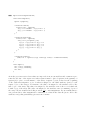
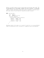
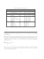
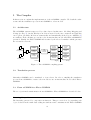
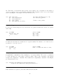
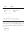
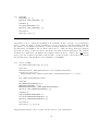
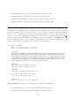
s-COMMA User’s Manual
Modeling Constraint Satisfaction Problems
Edition 0.1, for s-COMMA Version 0.1
August 2007
Ricardo Soto, Laurent Granvilliers
c 2004–2007 Laboratoire d’Informatique de Nantes Atlantique, France.
Copyright Ricardo Soto
Laboratoire d’Informatique de Nantes Atlantique
Université de Nantes
B.P. 92208, F-44322 Nantes cedex 3, France
[email protected]
Laurent Granvilliers
Laboratoire d’Informatique de Nantes Atlantique
Université de Nantes
B.P. 92208, F-44322 Nantes cedex 3, France
[email protected]
The authors hereby grant you non-exclusive and non-transferable license to use, copy and modify
this manual for non-commercial purposes.
Acknowledgements
We would like to thank Mathieu Albert, Thibault Le Port, Joris Meury and Éric Vépa for
their support on the development of the ECLiPSe translator. We are also grateful to Thomas
Douillard and Nicolas Berger for their work as beta testers.
i
Contents
1 Distribution
License . . . . . . . . . . . . . . . . . . . . . . . . . . . . . . . . . . . . . . . . . . . .
1
1
2 Installation
Software Requirements
Installation . . . . . .
Use of s-COMMA . .
Bug Report . . . . . .
.
.
.
.
3
3
3
3
3
.
.
.
.
.
.
.
.
5
5
5
6
6
7
8
9
11
.
.
.
.
.
.
.
.
.
.
.
.
.
.
.
.
.
.
15
15
15
15
15
15
16
16
17
17
18
19
19
20
20
20
21
22
23
.
.
.
.
25
25
25
25
27
.
.
.
.
.
.
.
.
.
.
.
.
.
.
.
.
.
.
.
.
.
.
.
.
.
.
.
.
.
.
.
.
.
.
.
.
.
.
.
.
.
.
.
.
3 Overview
Constraint Satisfaction Problems . .
Solver Independence . . . . . . . . .
3.1 Constraint Modeling by Examples .
Example: SEND+MORE=MONEY
Example: N-Queens . . . . . . . . .
Example: Perfect Squares . . . . . .
Example: Perfect Squares . . . . . .
Example: The Engine . . . . . . . .
4 Model Components
4.1 Constants . . . . . .
Integer constants . .
Real constants . . .
Enumerations . . . .
4.2 Attributes . . . . . .
Decision Variables .
Constrained Objects
4.3 Constraint Zones . .
Constraints . . . . .
Loops . . . . . . . .
Conditionals . . . . .
Optimization . . . .
Global Constraints .
Global Constraints .
4.4 Object Composition
4.5 Inheritance . . . . .
4.6 Extensibility . . . .
4.7 Limitations . . . . .
5 The
5.1
5.2
5.3
5.4
.
.
.
.
.
.
.
.
.
.
.
.
.
.
.
.
.
.
.
.
.
.
.
.
.
.
.
.
.
.
.
.
.
.
.
.
Compiler
Architecture . . . . . . .
Translation process . . .
From s-COMMA to Flat
From Flat s-COMMA to
.
.
.
.
.
.
.
.
.
.
.
.
.
.
.
.
.
.
.
.
.
.
.
.
.
.
.
.
.
.
.
.
.
.
.
.
.
.
.
.
.
.
.
.
.
.
.
.
.
.
.
.
.
.
.
.
.
.
.
.
.
.
.
.
.
.
.
.
.
.
.
.
.
.
.
.
.
.
.
.
.
.
.
.
.
.
.
.
.
.
.
.
.
.
.
.
.
.
.
.
.
.
.
.
.
.
.
.
.
.
.
.
.
.
.
.
.
.
.
.
.
.
.
.
.
.
.
.
.
.
.
.
.
.
.
.
.
.
.
.
.
.
.
.
.
.
.
.
.
.
.
.
.
.
.
.
.
.
.
.
.
.
.
.
.
.
.
.
.
.
.
.
.
.
.
.
.
.
.
.
.
.
.
.
.
.
.
.
.
.
.
.
.
.
.
.
.
.
.
.
.
.
.
.
.
.
.
.
.
.
.
.
.
.
.
.
.
.
.
.
.
.
.
.
.
.
.
.
.
.
.
.
.
.
.
.
.
.
.
.
.
.
.
.
.
.
.
.
.
.
.
.
.
.
.
.
.
.
.
.
.
.
.
.
.
.
.
.
.
.
.
.
.
.
.
.
. . . . . . . . . . . .
. . . . . . . . . . . .
s-COMMA . . . . .
native solver models
iii
.
.
.
.
.
.
.
.
.
.
.
.
.
.
.
.
.
.
.
.
.
.
.
.
.
.
.
.
.
.
.
.
.
.
.
.
.
.
.
.
.
.
.
.
.
.
.
.
.
.
.
.
.
.
.
.
.
.
.
.
.
.
.
.
.
.
.
.
.
.
.
.
.
.
.
.
.
.
.
.
.
.
.
.
.
.
.
.
.
.
.
.
.
.
.
.
.
.
.
.
.
.
.
.
.
.
.
.
.
.
.
.
.
.
.
.
.
.
.
.
.
.
.
.
.
.
.
.
.
.
.
.
.
.
.
.
.
.
.
.
.
.
.
.
.
.
.
.
.
.
.
.
.
.
.
.
.
.
.
.
.
.
.
.
.
.
.
.
.
.
.
.
.
.
.
.
.
.
.
.
.
.
.
.
.
.
.
.
.
.
.
.
.
.
.
.
.
.
.
.
.
.
.
.
.
.
.
.
.
.
.
.
.
.
.
.
.
.
.
.
.
.
.
.
.
.
.
.
.
.
.
.
.
.
.
.
.
.
.
.
.
.
.
.
.
.
.
.
.
.
.
.
.
.
.
.
.
.
.
.
.
.
.
.
.
.
.
.
.
.
.
.
.
.
.
.
.
.
.
.
.
.
.
.
.
.
.
.
.
.
.
.
.
.
.
.
.
.
.
.
.
.
.
.
.
.
.
.
.
.
.
.
.
.
.
.
.
.
.
.
.
.
.
.
.
.
.
.
.
.
.
.
.
.
.
.
.
.
.
.
.
.
.
.
.
.
.
.
.
.
.
.
.
.
.
.
.
.
.
.
.
.
.
.
.
.
.
.
.
.
.
.
.
.
.
.
.
.
.
.
.
.
.
.
.
.
.
.
.
.
.
.
.
.
.
.
.
.
.
.
.
.
.
.
.
.
.
.
.
.
.
.
.
.
.
.
.
.
.
.
.
.
.
.
.
.
.
.
.
.
.
.
.
.
.
.
.
.
.
.
.
.
.
.
.
.
.
.
.
.
.
.
.
.
.
.
.
.
.
.
.
.
.
.
.
.
.
.
.
.
.
.
.
.
.
.
.
.
.
.
.
.
.
.
.
.
.
.
.
.
.
.
.
.
.
.
.
.
.
.
.
.
.
.
.
.
.
.
.
.
.
.
.
.
.
.
.
.
.
.
.
.
.
.
.
.
.
.
.
.
.
.
.
.
.
.
.
.
.
.
.
.
.
.
.
.
.
.
.
.
.
.
.
.
.
.
.
.
.
.
.
.
.
.
.
.
.
.
.
.
.
.
.
.
.
.
.
.
.
.
.
.
.
.
.
.
.
.
.
.
.
.
.
.
.
.
.
.
.
.
.
.
.
.
.
.
.
.
.
.
.
.
.
.
.
.
.
.
.
.
.
.
.
.
.
.
.
.
.
.
.
.
.
.
.
.
.
.
.
.
.
.
.
.
.
.
Index
33
References
35
Grammar of the Language
37
Grammar of Flat-s-COMMA
43
iv
1
Distribution
s-COMMA 0.1
BSD License
Copyright (c) 2004–2007, Laboratoire d’Informatique de Nantes Atlantique (LINA), France
All rights reserved.
Redistribution and use in source and binary forms, with or without modification, are permitted
provided that the following conditions are met:
• Redistributions of source code must retain the above copyright notice, this list of conditions
and the following disclaimer.
• Redistributions in binary form must reproduce the above copyright notice, this list of conditions and the following disclaimer in the documentation and/or other materials provided
with the distribution.
• Neither the name of the LINA nor the names of its contributors may be used to endorse
or promote products derived from this software without specific prior written permission.
THIS SOFTWARE IS PROVIDED BY THE COPYRIGHT HOLDERS AND CONTRIBUTORS ”AS IS” AND ANY EXPRESS OR IMPLIED WARRANTIES, INCLUDING, BUT
NOT LIMITED TO, THE IMPLIED WARRANTIES OF MERCHANTABILITY AND FITNESS FOR A PARTICULAR PURPOSE ARE DISCLAIMED. IN NO EVENT SHALL THE
COPYRIGHT OWNER OR CONTRIBUTORS BE LIABLE FOR ANY DIRECT, INDIRECT,
INCIDENTAL, SPECIAL, EXEMPLARY, OR CONSEQUENTIAL DAMAGES (INCLUDING, BUT NOT LIMITED TO, PROCUREMENT OF SUBSTITUTE GOODS OR SERVICES; LOSS OF USE, DATA, OR PROFITS; OR BUSINESS INTERRUPTION) HOWEVER
CAUSED AND ON ANY THEORY OF LIABILITY, WHETHER IN CONTRACT, STRICT
LIABILITY, OR TORT (INCLUDING NEGLIGENCE OR OTHERWISE) ARISING IN ANY
WAY OUT OF THE USE OF THIS SOFTWARE, EVEN IF ADVISED OF THE POSSIBILITY
OF SUCH DAMAGE.
2
Installation
Software and Hardware Requirements
The compilation of s-COMMA requires Java 1.5 and Apache Ant. To date, s-COMMA is known
to compile on ix86 computers under Linux and Windows.
Installation
The installation of s-COMMA is done in two steps:
1. Put the zip file in a directory where you have write permissions and unpack it:
2. Enter the subdirectory and install:
% cd s-comma-0.1
% ant build
Use of s-COMMA
You should be able to call s-COMMA, using a target solver, by the following command:
% ./comma -gecodej examples/Send.cma
If the process succeeds, a solver-file will be generated in:
src/comma/solverFiles/
Launch this file using the corresponding solver. Libraries called by solver-files are provided in
the same folder. Solvers are not included in the distribution.
Help about the s-COMMA usage and launch options can be obtained with:
% ./comma -h
Bug Report
Please report bugs to Ricardo Soto by e-mail or by regular mail with subject “s-COMMA bug”.
Suggestions for improvement are most welcome.
LINA – Faculté des Sciences
2, rue de la Houssinière
B.P. 92208
44322 Nantes Cedex 3 – France
[email protected].
3
3
Overview
s-COMMA is a solver-independent language for modeling constraint satisfaction problems (CSP).
In this section, we describe how problems are modeled using s-COMMA.
Constraint Satisfaction Problems
A CSP is a problem composed by data variables, usually called constants, decision variables and
relations between the variables called constraints. The goal is to find values for the variables
that satisfy the constraints. For instance the logical relation,
x + y ≥ 0,
is a constraint. The pair of values x = 0 and y = 0 is a feasible solution since 0 + 0 ≥ 0. This
pair is declared consistent with respect to the constraint.
The process of searching the solutions is done by solvers, which consists in eliminating inconsistent values. Initially, a domain is associated to each variable, i.e., the set of possible values
a priori. Solvers implement domain reductions by means of consistency techniques and domain
splitting in order to branch the solutions.
Solver Independence
Solver Independence means to separate the modeling from the solving concerns. This technique
is implemented in a three layered architecture. A modeling layer, a mapping layer and a solving
layer. Models are stated in the modeling layer, the mapping tool translates the models into an
executable solver code and then the solving layer performs the solving process.
Gecode/J
Solver
ECLiPSe
Solver
Model
Mapping
Tool
RealPaver
Solver
GNU Prolog
Solver
Modeling
Modeling
Solving
Figure 1: Solver Independence
This architecture gives the possibility to plug-in new solvers and to process a same model with
different solvers, which is useful to learn which solver is the best for the model.
s-COMMA has been implemented using this technology. Currently, s-COMMA models can be
translated to ECLiPSe [5], Gecode/J [2], RealPaver [4] and GNUProlog [3]. We expect to extend
the list of supported solvers in further versions.
5
3.1
Constraint Modeling by Examples
In this section we present some of the basic features of s-COMMA by means of three well-known
Constraint-Based Problems. We begin with the SEND+MORE=MONEY puzzle.
Example: SEND+MORE=MONEY
The problem consists in finding distinct digits for the letters S, E, N, D, M, O, R, Y such that S
and M are different from zero and the equation SEN D + M ORE = M ON EY is satisfied.
In this problem, we may identify the following model information:
• 8 variables: S, E, N, D, M, O, R, Y are the decision variables whose values must be searched.
• 2 constraint:
– The equation SEN D + M ORE = M ON EY .
– all the variables must take different values.
The s-COMMA model for the problem is as follows. We define a class called Send, then we define
the 8 decision variables, each variable is represented by an integer type (int). Due to variables
represent digits, its domain must be into [0, 9]. Variables s and m have a [1, 9] domain, whose
values must be different from zero.
import Global.ext;
class Send{
int s in [1,9];
int e in [0,9];
int n in [0,9];
int d in [0,9];
int m in [1,9];
int o in [0,9];
int r in [0,9];
int y in [0,9];
constraint eq{
1000*s + 100*e + 10*n + d
+ 1000*m + 100*o + 10*r + e
= 10000*m + 1000*o + 100*n + 10*e + y;
alldifferent();
}
}
We define a constraint zone called eq to post the constraints of the problem. First, we place
1000∗s+100∗e+10∗n+d+1000∗m+100∗o+10∗r +e = 10000∗m+1000∗o+100∗n+10∗e+y
to represent the equation SEN D + M ORE = M ON EY ; and then we post the global constraint
alldifferent(), which is imported from the extension file Global.ext (details about extension
6
files are presented in Section 4.6). This constraint forces that all values defined in the class must
be different.
Example: N-Queens
The problem consists in placing N chess queens on an N x N chessboard such that none of them
is able to capture any other using the standard chess queen’s moves. A solution requires that
no two queens share the same row, column, or diagonal.
In this problem, we may identify the following model information:
• 1 constant: to determine the value of n.
• n variables: one decision variable for each queen to represent their row positions on the
chessboard.
• 3 constraint:
– To avoid that two queens are placed in the same row.
– To avoid that two queens are placed in the first diagonal.
– To avoid that two queens are placed in the second diagonal.
The s-COMMA model for the problem is as follows. We define a class called Queens, then
we define an array containing the n integer decision variables, each variable lies in [1, n]. The
constant value of n is imported from the Queens.dat file. A constraint zone called noAttack
contains the three constraints identified above. Two for loops ensures that the constraints are
applied for the complete set of decision variables.
♦♦♦ int n:=6;
import Queens.dat;
class Queens{
int q[n] in [1,n];
constraint noAttack{
for(i:=1;i<=n;i++){
for(j:=i+1;j<=n;j++){
q[i] <> q[j];
q[i]+i <> q[j]+j;
q[i]-i <> q[j]-j;
}
}
}
}
7
Example: Perfect Squares
The goal of this problem is to place a given set of squares in a square area. Squares may have
different sizes and they must be placed in the square area without overlapping each other.
In this problem, we may identify the following model information:
• 1 constant: to determine the size of the side of the area.
• 1 constant: to determine the quantity of squares to place in the area.
• square quantity constants: to determine the size of each square.
• 2 x square quantity variables: to determine the x and the y position of the squares.
• 2 constraint:
– To ensure that the x coordinate of the square is placed inside the area.
– To ensure that the y coordinate of the square is placed inside the area.
• 1 constraint: to ensure that the squares do not overlap with each other.
• 1 constraint: to ensure that the squares fit perfectly in the area.
A s-COMMA model for the Perfect Squares Problem is as follows. Three constant values are
imported from the data file , sideSize represents the side size of the square area where squares
must be placed, squares is the quantity of squares (8) to place and size is an array containing
the square sizes.
Two integer arrays of decision variables are defined to represent respectively the x and y coordinates of the square area. So, x[2]=1 and y[2]=1 means that the second of the eight squares
must be placed in row 1 and column 1, indeed in the upper left corner of the square area. Both
arrays are constrained, the decision variables must have values into the domain [1,sideSize].
A constraint zone called inside is declared. In this zone a forall loop contains the constraints
to ensure that each square is placed inside the area, one constraint about rows and the other
about columns.
The constraint noOverlap ensures that two squares do not overlap. The last constraint called
fitArea ensures that the set of squares fit perfectly in the square area.
♦♦♦ int sideSize:=5;
int squares:=8;
int size:=[3,2,2,2,1,1,1,1];
8
import PerfectSquares.dat;
class PerfectSquares{
int x[squares] in [1,sideSize];
int y[squares] in [1,sideSize];
constraint inside{
forall(i in 1..squares){
x[i] <= sideSize - size[i] + 1;
y[i] <= sideSize - size[i] + 1;
}
}
constraint noOverlap{
forall(i in 1..squares){
for(j:=i+1;j<=squares;j++){
x[i] + size[i] <= x[j] or
x[j] + size[j] <= x[i] or
y[i] + size[i] <= y[j] or
y[j] + size[j] <= y[i];
}
}
}
constraint fitArea{
(sum(i in 1..squares) (size[i]*size[i])) = sideSize*sideSize;
}
}
Example: An Object-Oriented version of the Perfect Squares
A main feature of the s-COMMA language is the capability of combining constraints with an
object-oriented framework. This kind of mix has been demonstrated to be useful for modeling
CSP whose structure is inherently hierarchic (see the Engine Problem). Besides, this feature
allow us to model in two different styles as we will show here giving a variant of the Perfect
Square Problem.
♦♦♦ int sideSize :=5;
int squares :=8;
Square PerfectSquares.s := [{_,_,3},{_,_,2},{_,_,2},{_,_,2},
{_,_,1},{_,_,1},{_,_,1},{_,_,1}];
9
import PerfectSquaresOO.dat;
class PerfectSquares{
Square s[squares];
constraint
forall(i
s[i].x
s[i].y
}
}
inside{
in 1..squares){
<= sideSize - s[i].size + 1;
<= sideSize - s[i].size + 1;
constraint noOverlap{
forall(i in 1..squares){
for(j:=i+1;j<=squares;j++){
s[i].x + s[i].size <= s[j].x or
s[j].x + s[j].size <= s[i].x or
s[i].y + s[i].size <= s[j].y or
s[j].y + s[j].size <= s[i].y;
}
}
}
constraint fitArea{
(sum(i in 1..squares) (s[i].size*s[i].size)) = sideSize*sideSize;
}
}
class
int
int
int
}
Square {
x in [1,sideSize];
y in [1,sideSize];
size;
As in the previous version, data values are imported from an external data file, sideSize represents the side size of the square area where squares must be placed, squares is the quantity of
squares (8) to place; s is an instance of the array of Square objects declared at the beginning
of the class PerfectSquares, a set of values is assigned to the third attribute (size) of each
Square object of the array s. For instance, the value 3 is assigned to the attribute size of the
first object of the array. The value 2 is assigned to the attribute size of the second, third and
fourth object of the array. The value 1 is assigned to the attribute size of remaining objects of
the array. We use standard modeling notation ( ) to omit assignments. Let us remark that we
can perform direct value assignment for attributes of a class in the data file (as we did for the
attribute size), this particularity gives us some benefits:
10
• Allow us to avoid the definition of constructors1 for each class.
• We do not need to call a constructor each time an object is stated. If we need to perform
an assignment we done it directly in the data file.
• Omitting these statements, we obtain a cleaner definition of classes.
At the PerfectSquares class, an array containing objects from the class Square is defined. This
class (declared at the end of the model) is used to model the set of squares. Attributes x and
y represent respectively the x and y coordinates. So, s[2].x=1 and s[2].y=1 means that the
second of the eight squares must be placed in row 1 and column 1. Both variables (x,y) lie in
[1,sideSize]. The last attribute called size represent the size of the square.
Constraint zones inside, noOverlap and fitArea carry out the same goal explained in the previous example.
Example: The Engine
Consider the task of configuring a car engine using a compositional approach (see Figure 2).
The engine at the first level is built from a crankcase, a cylinder system, a block and a cylinder
head at the second level. The cylinder system is a subsystem made of a valve system, a piston
system and an injection. Both valve and piston systems have their own composition rules.
Engine
Crankcase
Valve
Cylinder System
Cylinder Head
Block
Valve System
Injection
Piston System
Camshaft
Connecting Rod
Piston
Crankshaft
Figure 2: The Engine Problem
The Engine class is at the top of the hierarchy. The attributes cCase, cSyst, block and cHead
represent the subsystems of the engine. Those four constrained objects are instances of classes
to be declared. The last attribute volume defines the volume of the engine. Then, a constraint
between volume and the volume attribute of cCase is posted. The other classes and attributes
are described in the same way, for instance the CrankCase class below.
♦♦♦ enum size := {xsmall,small,medium,large,xlarge};
enum flow := {direct,indirect};
1
A constructor is a special function used to set up the class variables with values. It is used in most of
object-oriented programing languages.
11
import Engine.dat,
class Engine {
CrankCase cCase;
CylSystem cSyst;
Block
block;
CylHead
cHead;
int
volume in [890,4590];
constraint dim {
volume > cCase.volume;
}
}
class CrankCase {
size type;
int
oilVesselVol in [145,300];
int
bombePower in [255,400];
int
volume in [3890,6540];
}
The class CylSystem has a more complex declaration. The first attribute called quantity represents the quantity of cylinders; and the second represents the distance between cylinders. The
cylinder system has three subsystems denoted by inj, vSyst and pSyst. Then, a constraint
zone called determinePressure is declared to state a conditional constraint. This conditional
constraint represents that 6-cylinder-engines have a distance between cylinders bigger that 6.
In others kinds of engines the distance must be bigger than 3. In order to represent this constraint, an if-else statement is stated. If the condition is true, the first constraint is activated.
Otherwise, the second constraint is activated. The cSyst object declared in the Engine class can
be called a constrained object, due to it is an object subject to constraints on their attributes.
class CylSystem {
int
quantity in [2,12];
int
distBetCyl in [3,18];
Injection inj;
ValveSystem vSyst;
PistonSystem pSyst;
constraint determinePressure {
if (quantity = 6){
distBetCyl > 6;
}else{
distBetCyl > 3;
}
}
}
The subsystem injection is composed of three attributes called gasFlow, admValve, and pressure.
The decision variable gasFlow has a type called flow, which is an enumeration defined at the data
file. If an enumeration is used as a type for a decision variable, the decision variable adopts as domain the set of values of the enumeration. Thus, gasFlow adopts as domain {direct,indirect}.
12
Likewise, the variable admValve adopts as domain {xsmall,small,medium,large,xlarge}. The
injection class has also a compatibility constraint between its components. A compatibility
constraint limit the combination of allowed values for the decision variables to a given set. For
example, for variables type, admValve and pressure just four combination of values are allowed.
The possible values are described inside the compatibility built-in constraint.
class Injection {
flow
gasFlow;
size
admValve;
int
pressure in [80,130];
constraint compValues {
compatibility(type,admValve,pressure) {
("direct",
"small", 80);
("direct",
"medium", 90);
("indirect", "medium", 100);
("indirect", "large", 130);
}
}
}
Remaining elements of the engine are not presented because they do not present additional
features. Nevertheless, they can be view in the set of examples provided by the distribution.
13
4
Model Components
In the previous section we have shown the basic features of s-COMMA models by means of some
well-known examples. In this section we explain in more detail the components of models and
constructs supported by the language.
4.1
Constants
Constants, namely data variables, must be declared in a separate data file. Constants can be
real, integer or enumeration types.
Integer constants
s-COMMA allows integer variables, integer arrays and integer matrix. The declaration of each
one is as follows.
♦♦♦ int anIntegerConstant:=5;
int anArrayOfIntegerConstants:=[1,2,3];
int aMatrixOfIntegerConstants:=[[1,2,3],[1,2,3],[1,2,3]];
Real constants
The definition of real constants is the same as for integer constraints.
♦♦♦ real aRealConstant:=5.2;
real anArrayOfRealConstants:=[1.1,2.2,3.3];
real aMatrixOfRealConstants:=[[1.1,2.2,3.3],[1.1,2.2,3.3],[1.1,2.2,3.3]];
Enumerations
Enumerations can contain real, integer or string values. Enumerations are defined as follows.
♦♦♦ enum anEnumeration:={France, Italy, Germany};
4.2
Attributes
Attributes may represent decision variables or objects. Decision variables must be declared with
an Integer, Real or Boolean type. Objects must be typed with their class name.
15
Decision Variables
s-COMMA allows decision variables, arrays and matrix of decision variables. The size of the
arrays and matrix can be defined by a constant, an integer value or an expression. The expression
cannot contain decision variables, it must be composed by integers and/or constants.
int
real
bool
int
real
anIntegerDecisionVariable;
aRealDecisionVariable;
aBooleanDecisionVariable;
anArrayOfIntegerDecisionVariables[5];
aMatrixOfRealDecisionVariables[5,anIntegerConstant+1];
Variables, arrays and matrix may be constrained to a determined domain. The domain must be
defined with integer values for integer variables and real values for real variables. Constants and
expressions can be used for defining domains, but expressions cannot contain decision variables.
Attributes without domain adopt a default domain [-5000,5000] in the translation process2
int anIntegerDecisionVariable in [0,anIntegerConstant+1];
real aRealDecisionVariable in [0.5,5.5];
An enumeration can also be used as a type for a decision variable. The decision variable adopts
as domain the set of values of the enumeration.
♦♦♦ enum size:= {small, medium, large};
size sizeOfTheComponent;
Objects and Constrained Objects
Objects are instances of s-COMMA classes, which can be stated as attributes in models. Constrained Objects are objects subject to constraints on their attributes. The constrained object
firstEngine is shown below.
Engine firstEngine;
2
If you need to modify the default domain please refer to :
comma.control.managers.FeatManager.setDomainBounds()
16
4.3
Constraint Zones
Constraint zones are used to group constraints encapsulating them inside a class. A constraint
zone can contain constraints, loops, conditional statements, optimization statements, and global
constraints.
constraint inside{
forall(i in 1..squares){
x[i] <= sizeArea - size[i] + 1;
y[i] <= sizeArea - size[i] + 1;
}
}
Constraints
Constraint are relations between variables. Table 1 shows the operators supported by the constraints. E is an expression and N represents any numeric type. Let us notice that some
operators and types provided by s-COMMA are not supported by certain solvers, for details see
Section 4.7.
2 <= 4 + anIntegerDecisionVariable;
2 <= 5.4 - aRealDecisionVariable;
17
Table 1: Binary and Unary Operators
Operator
<->
->
<and
or
xor
<
>
<=
>=
==,=
!=,<>
+
*
/
-
Operation
Bi-Implication
Implication
Reverse Implication
Conjunction
Disjunction
Exclusive or
Less than
Greater than
Less than or equal
Greater than or equal
Equality
Inequality
Addition
Subtraction
Multiplication
Division
Numeric Negation
Precedence
1200
1100
1100
1000
900
900
800
800
800
800
800
800
400
400
300
300
150
Relation
(boolean × boolean) → boolean
(boolean × boolean) → boolean
(boolean × boolean) → boolean
(boolean × boolean) → boolean
(boolean × boolean) → boolean
(boolean × boolean) → boolean
(E × E) → boolean
(E × E) → boolean
(E × E) → boolean
(E × E) → boolean
(E × E) → boolean
(E × E) → boolean
(E × E) → N
(E × E) → N
(E × E) → N
(E × E) → N
N →N
Loops
s-COMMA provides the for loop and the forall loop. Loops can contain loops, conditionals
and constraints.
The for loop is declared as follows: The left side to declare the start value of the loop, the
middle part to declare the stop condition, and the right side to declare the increment of the
loop variable. Loop variables must not be declared, their validity begins when they are used to
define the start value of a loop (the loop variable i in the left side i:=1 ) and their validity finish
when their loop closes.
for(i:=1;j<=5;i++){
q[i] > i;
...
}
The forall loop is declared in two parts. The left part to define the loop variable and a right
part to define the set of values that the loop variable will traverse. The forall loop is always
performed in an incremental sense.
18
forall(i in 1..5){
q[i] > i;
...
}
There exist another way to declare the right part. Instead of defining a set of values, we can use
an enumeration or an array. The loop variable will cross from 1 until the size of the enumeration
or array.
forall(i in anEnumeration){
q[i] > i;
...
}
The sum loop performs an addition of a set of expressions. For example the expression a[1]*1 +
a[2]*2 + a[3]*3 can be compressed in the statement shown below.
sum(i in 1..5) (a[i]*i)
Let us note that parentheses around a[i]*i are mandatory.
Conditionals
Conditionals are stated by means of the if and the if-else. Due to the conditional is represented
by a logical formula, just one constraint is allowed inside the body of the conditional (we are
improving this for further versions).
if(a > b){
c > d;
else {
d < c;
}
Optimization
Optimization statements are defined with a tag specifying the kind of optimization to perform.
The [maximize] tag is used for maximizing and the [minimize] tag for minimizing expressions.
19
constraint reduce{
a + b > c;
[minimize] a + b;
}
Global Constraints
Two version of the alldifferent constraint are provided. The alldifferent(), forces that all
values defined in the class must be different and the alldifferent(anIntegerArray), forces that
all values inside an array must be different.
The alldifferent constraint is the unique global constraint included in the s-COMMA version
0.1, it is included as a extension of the language on a file called Global.ext. Additional global
constraints can be added using the extension mechanisms explained in Section 4.6.
Compatibility Constraints
As the explain in the Engine problem, a compatibility constraint limits the combination of
allowed values for a set of decision variables to a set of given tuples.
compatibility(a,b,c,d) {
(3, 5, 8, 6);
(1, 2, 5, 8);
(9, 0, 3, 2);
}
A compatibility constraint can be viewed as a logic formula. For instance the compatibility
constraint shown above can be represented by:
(a=3 and b=5 and c=8 and d=6) or
(a=1 and b=2 and c=5 and d=8) or
(a=9 and b=0 and c=3 and d=2)
4.4
Object Composition
The Object-Oriented framework provided by s-COMMA allows to represent models in an objectoriented style, as we shown by means of the Engine problem and the second version of the Perfect
Squares problem.
Let us remark that the main class of the model can be defined using the main reserved word. If
there is no main class in the model, the first class defined in the model will be set as the main
class.
20
main class Engine{
...
}
Object composition can be used to represent hierarchic models.
class Engine {
CrankCase cCase;
CylSystem cSyst;
Block
block;
CylHead
cHead;
...
}
Models can be stored in different files to be imported in a main file.
import examples.Engine.cma
import examples.ElectSystem.cma
...
class Car {
Engine
ElectricSystem
ExhaustSystem
SuspSystem
DriveTrain
Chassis
...
}
eng;
elSyst;
exSyst;
suSyst;
drSyst;
chass;
Let us note that recursion is not allowed between classes.
//not allowed
class Engine{
Engine eng;
}
4.5
Inheritance
Inheritance is allowed in s-COMMA. Using the reserved word extends a subclass inherits every
attribute and constraint defined in its superclass. Multiple inheritance is not allowed.
21
class TurboEngine extends Engine{
boost in [5,8];
...
}
4.6
Extensibility
One of the interesting aspects of s-COMMA is the capability of extending the constraint language. In order to explain this feature let us go back to the Perfect Squares Problem. Consider
that a Gecode/J programmer adds in the solver two new built-in functionalities: a constraint
called noOverlap and a function called sumArea. The constraint noOverlap will ensure that two
squares do not overlap and sumArea will sum the square areas of a square set. In order to use
these functionalities we need to extend the constraint language. To this end, we define a new
file (called extension file) where the rules of the translation are described.
GecodeJ {
Function {
sumArea(s) -> "sumArea($s$)";
}
Relation {
noOverlap(x,y,size,squares)
-> "noOverlap($x$, $y$, $size$, $squares$);";
}
}
ECLiPSe {
Function {
...
}
...
This file is composed by one or more main blocks (see code above). A main block defines the
solver where the new functionalities will be defined. Inside a main block two new blocks are
defined: a Function block and a Relation block.
In the Function block we define the new functions to add. In the example, the s-COMMA code
is sumArea. This function name will be used to call the new function from s-COMMA. The input
parameter of the new s-COMMA function is an array (s). Finally, the corresponding Gecode/J
code is given to define the translation. The new function will be translated to sumArea(s);.
Variables must be tagged with $ symbols.
In the Relation block we define the new constraints to add. In the example, a new constraint
called noOverlap is defined, it receives four parameters. The translation to Gecode/J is given.
Once the extension file is completed, it can be called by means of an import statement. The
resultant model using extensions is shown below.
22
import PerfectSquares.dat;
import PerfectSquares.ext;
class PerfectSquares {
x[squares] in [1,sideSize];
y[squares] in [1,sideSize];
constraint placeSquares {
forall(i in squares) {
x[i] <= sideSize - size[i] + 1;
y[i] <= sideSize - size[i] + 1;
}
noOverlap(x,y,size,squares);
sumArea(size) = sideSize*sideSize;
}
}
4.7
Limitations
Some features provided by s-COMMA are not supported by certain solvers. These limitations
are explained below:
• Gecode Translation
– The solver has been designed to support finite domain integer constraints, in consequence real types are not supported.
– Optimizations cannot be applied to a given set of variables, they are always performed
for the whole set of variables defined in the model.
• ECLiPSe Translation
– Optimizations are not supported for real types.
• GNU Prolog Translation
– Optimizations are not supported for real types.
– Matrix are not implemented yet.
• RealPaver Translation
– RealPaver is an interval software for modeling and solving nonlinear systems. Due
to the continuous nature of intervals of real numbers, it is in general not possible to
check the equality of values, and it is replaced with the membership operation. As a
consequence, just the symbols (<=), (=>), (=) are allowed.
23
5
The Compiler
In this section we explain the implementation of the s-COMMA compiler. We detail the architecture and the translation process from s-COMMA to solver models.
5.1
Architecture
The s-COMMA system is supported by a three layered architecture: Modeling, Mapping and
Solving (see Fig. 3). On the first layer, models are stated by the user, extension and data files
can be given optionally. Models are syntactically and semantically checked by two ANTLR [1]
tree-walkers. If the checking process succeeds, an intermediate model called Flat s-COMMA is
generated. Finally, the Flat s-COMMA file is taken by the selected translator which generates
the executable solver file.
Gecode/J
Translator
Extension
Compiler
Extension
File (Optional)
Base
Compiler
Gecode/J
Solver
ECLiPSe
Solver
ECLiPSe
Translator
Flat
s-COMMA
Compiler
Model
Data
Compiler
Data
File (Optional)
Modeling
RealPaver
Translator
RealPaver
Solver
GNU Prolog
Translator
GNU Prolog
Solver
Mapping
Solving
Figure 3: The s-COMMA compiling system.
5.2
Translation process
Currently s-COMMA can be translated to four solvers. In order to simplify the translation
process from s-COMMA to native solver models we use an intermediate model called Flat sCOMMA.
5.3
From s-COMMA to Flat s-COMMA
The set of performed transformation from s-COMMA to Flat s-COMMA are described below.
Flattening Composition
The hierarchy generated by composition is flattened. This process is done by expanding each
object declared in the main class adding its attributes and constraints in the Flat s-COMMA
25
file. The name of each attribute has a prefix corresponding to the concatenation of the names of
objects of origin in order to avoid name redundancy. The expansion of the object cCase defined
in the class Engine of the Engine Problem is shown below
♦♦♦ size
int
int
int
int
cCase_base;
cCase_oilVesselVol;
cCase_bombePower;
cCase_volume;
cSyst_quantity in [2,12];
int cSyst_distBetCyl in [3, 18];
flow cSyst_inj_gasFlow;
...
volume > cCase_volume;
Loop Unrolling
Loops are not widely supported by solvers, hence we generate an unrolled version of loops (for
and forall).
♦♦♦ //s-COMMA
forall(i in 1..3){
a[i] < a[i+1];
}
//flat
a[1] <
a[2] <
a[3] <
s-COMMA
a[2];
a[3];
a[4];
Conditional removal
Conditional statements are transformed to logical formulas. For instance, if a then b else c
is replaced to (a ⇒ b) ∩ (a ∪ c).
♦♦♦ //s-COMMA
if(a=b) c>=d;
else
c<d;
//flat s-COMMA
(a=b) -> (c>=d) and (a=b) or (c<d);
Compatibility removal
Compatibility constraints are also translated to a logical formula. We create a conjunctive
boolean expression for each n-tuple of allowed values. Then, each constraint of the n-tuple
is stated in a disjunctive constraint. The transformed compatibility constraint of the Engine
problem is shown below.
♦♦♦ ((type=1) and (admValve=1) and (pressure=80)) or
((type=1) and (admValve=2) and (pressure=90)) or ...
Data substitution
Data variables are replaced by its value defined in the data file.
26
Enumeration substitution
In general solvers do not support non-numeric types. So, enum types are replaced by integer values, for example admValve in {small,medium,large} is replaced by admValve in [1,3]; original
values are stored to give the results.
Array decomposition
Array containing objects are decomposed into single objects which are then expanded by the
flattening composition described above. For instance, in the perfect squares problem, the array
of objects called s is decomposed as follows:
♦♦♦ int s_1_x in [1,5];
int s_1_y in [1,5];
int s_2_x in [1,5];
int s_2_y in [1,5];
int s_3_x in [1,5];
...
The name of each variable is composed by the name of the array s, the position of the object in
the array, and the name of the attribute of the object. Only, variables x and y are considered
decision variables, the attribute size is considered constant due to has an instantiation (in the
data file at line 3) for the whole set of objects contained in the array. The value 5 in the variables’
domain comes from the data substitution of the data variable sideSize.
Logic formulas transformation
Some logic operators are not supported by solvers. For example logical equivalence (a ⇔ b) and
reverse implication (a ⇐ b). We transform logical equivalence expressing it in terms of logical
implication ((a ⇒ b) ∩ (b ⇒ a)). Reverse implication is simply inversed (b ⇒ a).
5.4
From Flat s-COMMA to native solver models
After the generation of the intermediate model, the Flat s-COMMA code is taken by the selected
translator which generates the executable solver file.
Single Data translation
The data substitution process performed in the intermediate model generation replaces all the
data variables with its corresponding value, so data is no longer needed in solver files. But
specific extension could need it, so we give a data translation for solver files.
27
♦♦♦ //flat s-COMMA
aConstant:=5;
//ECLiPSe
ACONSTANT=5,
//Gecode/J
aConstant n=5;
//GNUPROLOG
ACONSTANT=5,
//RealPaver
aConstant=5,
Data Array translation
♦♦♦ //flat s-COMMA
anArrayOfConstants:=[1,2,3];
//Gecode/J
int anArrayOfConstants[]={1,2,3},
//GNUPROLOG
ANARRAYOFCONSTANTS=[](1,2,3),
//RealPaver
anArrayOfConstants=[1,2,3],
//ECLiPSe
ANARRAYOFCONSTANTS=[](1,2,3),
Additional information can be regarded in the sources of the distribution:
• comma.translators.gecodej.GecodeJDataVarsCodeGenerator.java
• comma.translators.eclipse.EclipseDataVarsCodeGenerator.java
• comma.translators.gnuprolog.GNUPrologDataVarsCodeGenerator.java
• comma.translators.realpaver.RealPaverDataVarsCodeGenerator.java
Single Variable translation
Variables are mapped to their equivalent ones in solver languages. For instance in Gecode/J the
object IntVar is used to define a decision variable, this represents the Java Space of Gecode/J,
"aVariable" the name of the variable, and finally its domain ([2,5]) is defined. Then, the
variable is added to a specific array for the labeling process (labeling-array). In ECLiPSe the
variable is defined including its domain using the (::) notation. As in Gecode/J the variable is
added to the labeling-array. The variable declaration for GNUProlog is performed by means of
the fd domain predicate. Then, the variable is added to the labeling-array. The RealPaver case
no needs explanation.
♦♦♦ //flat s-COMMA
int aVariable in [2,5];
//Gecode/J
IntVar aVariable = new IntVar(this,"aVariable",2,5);
vars.add(aVariable);
28
♦♦♦ //ECLiPSe
AVARIABLE::[2..5],
append([],VARS_AVARIABLE_,L_),
//GNUProlog
fd_domain(AVARIABLE,2,5),
append([],VARS_AVARIABLE_,L_),
//RealPaver
aVariable in [2,5],
Variable Array translation
Arrays have a more complicated translation. For instance in Gecode/J the object VarArray is
used to define an array of decision variables, a for loop is used to fill the VarArray with the
five IntVar objects which represent the decision variables, finally the new array is added to the
labeling-array. In ECLiPSe the predicate dim is used to define an array, then its domain is
given, the two last code lines are used to insert the new array in the labeling-array. The variable
declaration for GNUProlog is similar, the length predicate is used to define a list, fd domain is
used to give the domain of its values, and the last code line is given to insert the new array in
the labeling-array. The RealPaver case is similar to s-COMMA.
♦♦♦ //flat s-COMMA
int anArrayOfVariables[5] in [3,8];
//Gecode/J
VarArray<IntVar> anArrayOfVariables = new VarArray<IntVar>();
for(int i=1;i<=5;i++) {
anArrayOfVariables.add(new IntVar(this,"anArrayOfVariables" + i,3,8));
}
vars.addAll(anArrayOfVariables);
//ECLiPSe
dim(ANARRAYOFVARIABLES,[5]),
ANARRAYOFVARIABLES::[3..8],
ANARRAYOFVARIABLES=[_|VARS_ANARRAYOFVARIABLES_]
append([],VARS_ANARRAYOFVARIABLES_,L_),
//GNUProlog
length(ANARRAYOFVARIABLES,5)
fd_domain(ANARRAYOFVARIABLES,3,8),
append([],ANARRAYOFVARIABLES,L_X_),
//RealPaver
aVariable[1..5] in [3,8],
Additional information can be regarded in the sources of the distribution:
29
• comma.translators.gecodej.GecodeJDecVarsCodeGenerator.java
• comma.translators.eclipse.EclipseDecVarsCodeGenerator.java
• comma.translators.gnuprolog.GNUPrologDecVarsCodeGenerator.java
• comma.translators.realpaver.RealPaverDecVarsCodeGenerator.java
Constraint translation
Constraints are translated in a very different way depending on the nature of the solvers’ language. For instance in Gecode/J, methods are used to define constraints, the post method is
used to post a constraint, the p method represents the addition operator. The BExpr object is
given to post boolean expressions, the Expr object is used to post math expressions, and IRT LQ
represents the <= relation. ECLiPSe and GNU Prolog cases are similar to s-COMMA , in GNU
the predicate nth is used to get a variable of the array. As we explain previously, due to the
nature of the RealPaver solver it does not support the or operator.
♦♦♦ //flat s-COMMA
x[1] + 3 <= x[2] or x[2] + 2 <= x[1] or
y[1] + 3 <= y[2] or y[2] + 2 <= y[1];
//Gecode/J
post(this,new BExpr(new BExpr(new BExpr( new Expr().p(new Expr().p(get(x,1))).
p(new Expr().p(3)),IRT_LQ, new Expr().p(get(x,2))).or(new BExpr( new Expr().
p(new Expr().p(get(x,2))).p(new Expr().p(2)),IRT_LQ, new Expr().p(get(x,1))))).
or(new BExpr( new Expr().p(new Expr().p(get(y,1))).p(new Expr().p(3)),IRT_LQ,
new Expr().p(get(y,2))))).or(new BExpr( new Expr().p(new Expr().p(get(y,2))).
p(new Expr().p(2)),IRT_LQ, new Expr().p(get(y,1)))));
//ECLiPSe
X[1]+3 $=< X[2] or X[2]+2 $=< X[1] or
Y[1]+3 $=< Y[2] or Y[2]+2 $=< Y[1],
//GNUPROLOG
nth(1,X,X_1),nth(2,X,X_2),nth(3,X,X_3)...
X_1+3 #=< X_2 #\/ X_2+2 #=< X_1 #\/
Y_1+3 #=< Y_2 #\/ Y_2+2 #=< Y_1,
//RealPaver
x[1] + 3 <= x[2]...// or not supported
Additional information can be regarded in the sources of the distribution:
• comma.translators.gecodej.GecodeJConstraintCodeGenerator.java
• comma.translators.eclipse.EclipseConstraintCodeGenerator.java
30
• comma.translators.gnuprolog.GNUPrologConstraintCodeGenerator.java
• comma.translators.realpaver.RealPaverConstraintCodeGenerator.java
Formatters
The name of the decision variables as well as the name of data variables need in general to
be formatted for the specific syntax of the solver. This task is performed respectively by the
following source codes:
• comma.translators.gecodej.GecodeJFormatter.java
• comma.translators.eclipse.EclipseFormatter.java
• comma.translators.gnuprolog.GNUPrologFormatter.java
• comma.translators.realpaver.RealPaverFormatter.java
Headers
Executable solver files need often specific headers to call libraries, procedures and/or to show
the results in an adequate way. These tasks are performed respectively by the following source
codes:
• comma.translators.gecodej.GecodeJTranslator.java
• comma.translators.eclipse.EclipseTranslator.java
• comma.translators.gnuprolog.GNUPrologTranslator.java
• comma.translators.realpaver.RealPaverTranslator.java
31
Index
alldifferent, 20
architecture, 25
attributes, 15
compatibility, 20
compiler, 25
component, 20
composition, 20
conditional, 19
consistency technique, 5
consistent, 5
consistent value, 5
constant, 5, 15
array, 15
enumeration, 15
integer, 15
matrix, 15
real, 15
constrained object, 11, 16
constraint, 5, 17
Constraint Programming, 5
Constraint Satisfaction Problem, 5
constraint zone, 17
CSP, 5
minimize, 19
object, 16, 20
operator
binary, 17
unary, 17
optimization, 19
search, 5
solver, 5
Solver Independence, 5
sum, 18
variable
array, 15, 25
boolean, 15, 25
integer, 15, 25
matrix, 15, 25
real, 15, 25
data variable, 15
decision variable, 15
decision variables, 5
domain, 5
extensibility, 22
extensions, 22
feasible solution, 5
for, 18
forall, 18
global constraint, 20
if, 19
if-else, 19
inheritance, 21
loop, 18
maximize, 19
33
References
[1] ANTLR Reference Manual. http://www.antlr.org.
[2] Gecode System. http://www.gecode.org.
[3] Daniel Diaz and Philippe Codognet. The gnu prolog system and its implementation. In SAC
(2), pages 728–732, 2000.
[4] L. Granvilliers and F. Benhamou. Algorithm 852: Realpaver: an interval solver using constraint satisfaction techniques. ACM Trans. Math. Softw., 32(1):138–156, 2006.
[5] M. Wallace, S. Novello, and J. Schimpf. Eclipse: A platform for constraint logic programming, 1997.
35
36
Grammar of the Language
The grammar is described by means of EBNF using the following conventions: Angle brackets are
used to denote non-terminals (e.g. hClass-Bodyi). Bold font and underlined bold font are used
to denote terminals (e.g. class, ;). Square brackets denotes optional items (e.g.[hArray-Dimi]).
Square brackets with a plus symbol defines sequences of one or more items (e.g.[hClassi]+ ).
Square brackets with a star symbol are used for sequences of zero or more items (e.g. [hImporti]∗ ).
Program
hProgrami ::= [hImporti]∗ [hClassi]+
hImporti ::= import hPathi;
hClassi ::= class hClass-Namei [extends hClass-Namei] {hClass-Bodyi}
hClass-Bodyi ::= [hAttributei;]∗ [hConstraint-Zonei]∗
hPathi ::= [hFolder-Namei.]∗ hFile-Namei
Attributes
hAttributei ::= hDecision-Var i | hConstrained-Objecti
hDecision-Var i ::=
hTypei hVar-Namei
| hDecision-Var-Assigned i
| hDecision-Var-Constrained i
| hDecision-Var-Arrayi
| hDecision-Var-Array-Constrained i
hConstrained-Objecti ::= hClass-Namei hVar-Namei
hDecision-Var-Assigned i ::= hTypei hVar-Namei := hexpressioni
hDecision-Var-Constrained i ::= hTypei hVar-Namei in hinterval i | hseti
hDecision-Var-Arrayi ::= hTypei hVar-Namei hArray-Dimi
hDecision-Var-Array-Constrained i ::= hTypei hVar-Namei hArray-Dimi in hinterval i | hseti
Constraints
hConstraint-Zonei ::= constraint hConstraint-Namei {hConstraint-Bodyi}
hConstraint-Bodyi ::= [hConstraint-Def i]∗
hConstraint-Def i ::=
hFor i
| hForall i
| hIf-Elsei
| hDomaini hConstrainti;
| hOptimizationi
| hBuilt-In-Constrainti
37
hConstrainti ::= hConstraintihBool-OpihConstrainti | hRel-Expressioni
hBool-Opi ::= or | and | xor | -> | <- | <->
hRel-Expressioni ::= hRel-ExpressionihRel-OpihRel-Expressioni | hMath-Expressioni
hRel-Opi ::= < | <= | > | >= | = | <>
Expressions
hMath-Expressioni ::=
|
|
|
|
hMath-Expressioni hMath-Opi hMath-Expressioni
hBuilt-In-Functioni
hAccessi
hLiteral i
hMath-Opi ::= + | - | * | /
hAccessi ::= [hVar-Namei[hArray-Dimi].]∗ hVar-Namei [hArray-Dimi]
hArray-Dimi ::= [hInt-Literal i | hVar-Namei] [[ hInt-Literal i | hVar-Namei]]
Statements
hForall i ::= forall( hLoop-Var i in hValue-Seti) {hConstraint-Bodyi}
hValue-Seti ::= hVar-Namei | hInt-Literal i .. hVar-Namei
hFor i ::= for(hFor-Starti;hFor-Cond i;hIncr i |hDecr i) { hConstraint-Bodyi}
hFor-Starti ::= hLoop-Var i:=hInt-Expressioni
hFor-Cond i ::= hLoop-Var ihRel-OpihInt-Expressioni
hIf-Elsei ::= if (hConstrainti) {hConstrainti} [else{hConstrainti}]
hOptimizationi ::= hOpt-Valuei hMath-Expressioni ;
hOpt-Valuei ::= [ maximize ] | [ minimize ]
hTypei ::= int | real | bool
hInterval i ::= [hInt-Literal i | hVar-Namei, hInt-Literal i | hVar-Namei]
| [hReal-Literal i | hVar-Namei, hReal-Literal i | hVar-Namei]
hArray-Brai ::= [][[]]
hSeti ::= {hsetItemi[, hsetItemi]∗ }
hLiteral i ::= hInt-Literal i | hReal-Literal i | hBool-Literal i | hString-Literal i
hIncr i ::= hLoop-Var i + +
hDecr i ::= hLoop-Var i - -
38
Identifiers
hFolder-Namei
hFunction-Namei
hFile-Namei
hClass-Namei
hConstraint-Namei
hVar-Namei
hLoop-Var i
hSolver-Namei
::=
::=
::=
::=
::=
::=
::=
::=
hidenti
hidenti
hidenti
hidenti
hidenti
hidenti
hidenti
hidenti
Data
hDatai ::= [hConstanti | hInstancei]∗
hConstanti ::=
hVector-Datai ::=
hEnum-Datai ::=
hMatrix-Datai ::=
hInstancei ::=
hObjecti
hVector-Objecti
hMatrix-Objecti
hUnderscorei
::=
::=
::=
::=
hVar-Namei
:= hLiteral i | hVector-Datai | hMatrix-Datai | hEnum-Datai
[ hLiteral i [, hLiteral i]∗ ]
{ hLiteral i [, hLiteral i]∗ }
[ hArray-Datai | [, hArray-Datai]∗ ]
hAccessi
:= hObjecti | hVector-Objecti | hMatrix-Objecti
{ hLiteral i|hUnderscorei [, hLiteral i|hUnderscorei]∗ }
[ hObjecti [, hObjecti]∗ ]
[ hVector-Objecti | [, hVector-Objecti]∗ ]
Extensions
hExtensioni ::= [hExtension-Block i]∗
hExtension-Block i ::= hSolver-Namei { [hFunction-Block i] [hRelation-Block i] }
hFunction-Block i ::= Function{[hFunctioni ;]∗ }
hRelation-Block i ::= Relation{[hRelationi ;]∗ }
hFunctioni ::= hComma-Codei -> hSolver-Codei
hRelationi ::= hComma-Codei -> hSolver-Codei
hComma-Codei ::= " hidenti ( [hInput-Parametersi] ) "
hInput-Parametersi ::= hParameter i [, hParameter i ]∗
hParameter i ::= hVar-Namei [hArray-Brai]
hSolver-Codei ::= " [hString-Literal i]∗ | [hSolver-Var i]∗ "
hSolver-Var i ::= $ hString-Literal i $
Built-in Constraints
hBuilt-In-Constraintsi ::=
hCompatibilityi
| hNew-Built-In-Constraintsi
39
hCompatibilityi ::= compatibility (hAccessi[ ,hAccessi]∗ ) {[hValid-Tuplesi]+ }
hValid-Tuplesi ::= (hLiteral i[ ,hLiteral i]∗ )
hNew-Built-In-Constraintsi ::= ident ( [hInput-Parametersi] ) ;
Built-in Functions
hBuilt-In-Functionsi ::=
hSumi
| hNew-Built-In-Functioni
hSumi ::= sum( hLoop-Var i in hValue-Seti) (hInt-Expressioni | hReal-Expressioni)
hNew-Built-In-Functioni ::= ident ( [hInput-Parametersi] )
40
42
Grammar of Flat-s-COMMA
The grammar is described by means EBNF using the following conventions: Angle brackets are
used to denote non-terminals (e.g. hClass-Bodyi). Bold font and underlined bold font are used
to denote terminals (e.g. attributes:, ;). Square brackets denotes optional items (e.g.[not]).
Square brackets with a plus symbol defines sequences of zero or more items (e.g.[hAttributei;]∗ ).
Program
hProgrami ::= attributes: [hAttributei;]∗ constraints: [hConstrainti;]∗
Attributes
hAttributei ::=
hTypei hIdenti
| hDecision-Var-Constrained i
| hDecision-Var-Arrayi
| hDecision-Var-Array-Constrained i
hDecision-Var-Constrained i ::= hTypei hIdenti in hinterval i
hDecision-Var-Arrayi ::= hTypei hIdenti hArray-Dimi
hDecision-Var-Array-Constrained i ::= hTypei hIdenti hArray-Dimi in hinterval i
Constraints
hConstrainti ::= hRel-Expr i[hBool-OpihRel-Expr i]∗
hBool-Opi ::= or | and | xor | -> | <- | <->
hRel-Expr i ::= hSum-Expr i[hRel-OpihSum-Expr i]∗
hRel-Opi ::= < | <= | > | >= | = | <>
hSum-Expr i ::= hMult-Expr i[hSum-Opi hMult-Expr i]∗
hSum-Opi ::= + | hMult-Expr i ::= hUnit-Expr i[hMult-Opi hUnit-Expr i]∗
hMult-Opi ::= * | /
hUnit-Expr i ::= [+] hNot-Expr i | - hNot-Expr i
hNot-Expr i ::= [not] hIdenti [hArray-Dimi] | [not] hLiteral i
hArray-Dimi ::= [hInt-Literal i | hIdenti [, hInt-Literal i | hIdenti]]
hTypei ::= int | real | bool
hInterval i ::= [hInt-Literal i , hInt-Literal i ] | [hReal-Literal i , hReal-Literal i ]
hLiteral i ::= hInt-Literal i | hReal-Literal i
hInt-Literal i ::= hInt-Literal i
43