1
AT&T Bell Laboratories
Murray Hill, New Jersey 07974
Computing Science Technical Report No. 103
IDEAL User’s
Manual
Christopher J. Van Wyk
December 17, 1981
IDEAL User’s
Manual
Christopher J. Van Wyk
AT&T Bell Laboratories
Murray Hill, New Jersey 07974
ABSTRACT
IDEAL
is a programming language to be used for describing pictures.
The main use of IDEAL is as a preprocessor to TROFF, so that pictures and
text may reside in the same file and be typeset together. This manual contains
many examples of this use of IDEAL.
IDEAL proper produces device-independent descriptions of pictures, so pictures may also be displayed through the UNIX plot filters.
This document describes how to use the existing implementation of IDEAL.
December 17, 1981
IDEAL User’s
Manual
Christopher J. Van Wyk
AT&T Bell Laboratories
Murray Hill, New Jersey 07974
1. Introduction
IDEAL is a language for describing pictures. It is intended primarily to operate as a preprocessor to TROFF[3], much like EQN TBL[2], REFER[0], and PIC
I have explained the principles that motivate the form of IDEAL elsewhere This document
describes how to use the existing implementation of IDEAL and treats several examples in depth.
Paragraphs like this that appear in smaller type may be skipped on first reading: they present
sidelights that may be ignored safely by beginners.
2. Overview of IDEAL
To take advantage of IDEAL’s capabilities, you must believe that
complex numbers are good.
•
Complex numbers have a natural correspondence to points in the Cartesian (x − y) coordinate system.
•
Using complex numbers obviates the need for distinguishing between ‘‘points’’ and
‘‘dimensions.’’
•
Complex numbers capture readily such common operations as translation, rotation, and
reflection in the plane.
programs define pictures by means of a system of simultaneous equations in the significant
points of the picture and a set of drawing instructions to be carried out with respect to those
points. IDEAL solves the system of equations, then draws the picture using the points so determined.
IDEAL
All variables in IDEAL programs are complex numbers, with the usual operations:
•
component-wise addition and subtraction: (a,b) ± (c,d) = (a±c,b±d)
•
vector multiplication: (a,b) *(c,d) = (ac − bd,ad + bc)
•
vector division: (a,b)/(c,d) = (ac + bd, − ad + bc)/(c 2 + d 2 )
•
component manipulation: re ( (a,b) ) = a, im ( (a,b) ) = b, and conj ( (a,b) ) = (a, − b)
•
vector magnitude calculation: abs ( (a,b) ) =
•
unit vector function: cis (θ) = cosθ + isinθ
√
a2 + b2
A non-standard notation that has proved useful is α[x,y], for complex x and y, defined by
x + α(y − x), and meaning ‘‘α of the way from x to y.’’
Scalars are treated as vectors with null imaginary component. For example, ‘‘1’’ is treated
as ‘‘(1,0).’’
The scale of the coordinate system in which IDEAL programs are written is entirely a matter
of convenience. The IDEAL processor proper produces output in the same coordinate system as
the input. Postprocessors (‘‘filters’’) scale this coordinate system to make sense for the device on
which the picture is displayed.
Some of the pictures below include captions keyed to the associated programs. Some of the
labels are not produced by the program: I added them to help explain the picture. Such labels are
-2-
parenthesized. For pictures and programs that have not been labeled, you may find that labeling
them yourself helps you understand the program.
3. Elements of the IDEAL Language
This section presents statements that make up the fundamental units of IDEAL programs, so
the displayed program text represents fragments of complete programs. Text that appears
between / * and * / is a comment.
3.1. Boxes
The building blocks of IDEAL programs are called boxes, which readers familiar with programming may think of as procedures or subroutines. In fact, the picture drawn by an IDEAL program must itself be a box, called main; we suppress this extra level of box-nesting for all of Section 3.
3.1.1. Defining Boxes
Here is a simple box and one instance of it:
rect {
(nw) ________ (ne)
(sw) ________(se)
var ne, nw, se, sw,
wd, ht;
nw = sw + (0,1)*ht;
ne = nw + wd;
se = sw + wd;
conn ne to nw to sw to se to ne;
}
It is called rect, has six local complex variables: ne, nw, se, sw, wd, and ht, three equations among
these variables, and an instruction to draw four lines.
3.1.2. Placing Boxes
To ask for an instance of rect, we use a put statement with a parameter section containing
enough additional equations that the local variables of this instance of rect are determined
uniquely. For example, we might give the dimensions (ht and wd) and one of the corners (say
sw):
____
put rect {
ht = 2;
wd = 1;
____
sw = 0;
};
Any of the following put statements would draw the same rectangle: (C programmers will recognize the / * and * / comment brackets.)
/* giving one corner, one dimension
and a relation on the dimensions */
put rect {
ht = 2;
wd = 0.5*ht;
nw = (0,2);
};
-3-
/* giving two adjacent corners
and the perpendicular dimension */
put rect {
nw = (0,2);
sw = 0;
wd = 1;
};
/* giving two diagonal corners
and a relation on the dimensions */
put rect {
ne = (1,2);
sw = 0;
wd = 0.5*ht;
};
/* giving three corners */
put rect {
ne = (1,2);
nw = (0,2);
se = 1;
};
/* giving the center of a side,
a corner, and another dimension */
put rect {
(nw+sw)/2 = (0,1);
nw = (0,2);
wd = 1;
};
The put statement is to IDEAL what a procedure call is to a conventional programming language.
The difference is that none of the variables of a box must be specified to be a parameter whose
value is expected in any call: any of the box’s variables may be set by the put statement, and
IDEAL will determine the rest by means of the equations in the definition of the box. This means
we can give whatever information we know about this instance of the box, as long as it is enough
to determine everything uniquely. This mechanism is useful because we often want to set down
a rectangle by giving one of its corners, but not necessarily the same corner each time; in a conventional programming language, we would need to provide a different procedure for each corner, and the code to solve for the other corners from it. (Almost certainly, not all of the put statements above are equally useful; but it is good to be able to use any of them when the need arises.)
Here is how IDEAL solves the system of equations implicit in a program: First, all equations are
placed on a queue. Every time a box is called, the solutions to these equations may—and probably will—be different, so all the equations of a box are enqueued separately for each time that
box is put. (Of course, different copies of the equation refer to different copies of the variable,
but IDEAL keeps that straight.) During processing, IDEAL maintains two classes of variables:
dependent and independent. Each dependent variable is represented as a linear combination of
independent variables plus a constant term. (Variables whose values are known are a trivial
case of dependent variables.) All variables start out independent. As long as there are equations on the queue, IDEAL examines the head equation: if, after substituting for all dependent
variables, the equation is linear, IDEAL determines new information from it if possible—that is,
IDEAL tries to make one variable dependent on the others, thus reducing the number of independent variables—or decides whether it is redundant or inconsistent; if the equation remains
non-linear after substitution, IDEAL adds it to the end of the queue and proceeds. If IDEAL ever
goes through the whole queue without discovering any new information, the system cannot be
solved (by IDEAL, anyway) and IDEAL complains bitterly. If there are any independent variables
left after this processing, IDEAL will complain too, because there is no way they can become
-4-
known.
The variables wd and ht above are complex numbers just like the corners, so we can rotate
the rectangle by giving them complex non-real values:
put rect {
sw = 0;
wd = (1,1)/abs((1,1));
ht = 2*wd;
};
(The double parentheses are needed in ‘‘abs( ( 1 , 1 ) ) ′ ′ because ‘‘abs( 1 , 1 )’’ is parsed as a function
with two arguments.) One point about this example often confuses new users: the vectors wd
and ht point in the same direction. It is in the definition of rect that the ht vector is rotated ninety
degrees and added to the southern points to arrive at the northern points. Thus, if we give a ht
that is perpendicular to wd, we get a very flat rectangle.
On the other hand, the definition of rect does not assure that ht and wd will point in the
same direction. This put statement draws a parallelogram:
put rect {
ht = 1;
wd = (1,1)/abs((1,1));
sw = 0;
};
Some people who feel that a box called rect should draw only rectangles are disturbed by this
example. One remedy is to add another equation to the definition of rect, asserting that two adjacent sides are perpendicular; IDEAL will complain if this equation is not satisfied (although it
won’t stop drawing). One such equation is
wd/abs(wd) = ht/abs(ht);
Here is a definition for box arrow that keeps the head of the arrow symmetrical about its
shaft:
arrow {
var hd, tl, head, wing;
head = 0.1;
wing = head*(tl-hd)/abs(tl-hd);
conn hd to tl;
conn hd + cis(25)*wing to hd to hd + cis(-25)*wing;
}
Note the definition of wing in the example above: the second part of the expression is a unit vector that points from tl to hd; this is multiplied by head, the length of the ‘‘wings’’ on the arrowhead.
When a put statement is interpreted, the equations in its parameter section are processed before
the equations in its definition. Thus, if there are inconsistent equations between the put statement and the box definition, the equations in the put statement take precedence. This can be
useful to provide default values for variables of a box. For instance, if the definition of rect
gave such default values to ht and wd, they would take effect unless overridden by equations in
the parameter section of the put statement.
ignores inconsistent equations, but it does generate error messages about them. To avoid
this error message about a particular equation, use a tilde (‘‘˜’’) instead of an equals sign in the
equation. The tilde does not give the equation any lower ‘‘priority’’ than an equation with an
equals sign: all it does is shut off the error message. So, the two ordered systems ‘‘x = 1, x ˜ 2’’
and ‘‘x ˜ 2, x = 1’’ are different: in the former, x receives the value 1, and no error message
appears when the second equation is processed; in the latter, x receives the value 2, and an
error is generated when the second equation is encountered.
IDEAL
-5-
3.2. Special Boxes—Circles and Arcs
Boxes to draw circles and circular arcs are defined in special library files.
3.2.1. Circles
The box named circle has five local variables: center, radius, z1, z2, and z3. The last three
may be any points on the circle. As above, we must give enough information to determine a circle; giving two points on it is insufficient, and giving three collinear points is inconsistent. Here
are three ways to draw a circle of radius one centered at the origin.
(z2)
/* giving center and radius */
put circle {
center = 0;
radius = 1;
};
(z1)
(z3)
/* giving center and a point on the circle */
put circle {
center = 0;
z1 = 1; /* could also have given z2 or z3 */
};
/* giving three points on the circle */
put circle {
z1 = (1,0);
z2 = cis(135);
z3 = cis(235);
};
Once the circle has been determined, all five of its internal variables are known. So, if we ask for
a circle giving three points, the radius and center will be known afterward. On the other hand, if
we ask for a circle by giving the center and the radius, the three points z1, z2, and z3, will be
known, and will be on the circle, but there is no guarantee where they will be.
3.2.2. Arcs
Box arc has eight local variables: center, radius, start, midway, end, startang, midang, and
endang. It is an arc centered at point center with radius radius, starting at point start at an angle
startang, passing through point midway at an angle midang, and ending at point end at an angle
endang. (All angles are measured with respect to center, in degrees, with the positive x-axis taken
to be zero degrees, and the counterclockwise direction to be positive.) Note that midway is not
necessarily the midpoint of the arc! If neither midway nor midang is given, the arc is drawn counterclockwise from start to end. Once again, a variety of put statements draw the same arc:
/* giving center, radius, and
starting and ending angles */
put arc {
center = 0;
radius = 1;
startang = 0;
endang = 235;
};
(midway)
(start)
(end)
-6-
/* giving center, starting point,
and ending angle */
put arc {
center = 0;
start = 1;
endang = 235;
};
/* giving three points on the arc */
put arc {
(midway)
start = cis(235);
midway = -1;
end = 0;
};
(end)
(start)
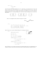
3.3. Other Elements of IDEAL Pictures
IDEAL
pictures also may contain text and splines.
3.3.1. Text Captions
There are three commands to place text with respect to a point. The left command leftjustifies the text with respect to the specified location: the text will start there. The right command right-justifies the text so that it ends at the specified location. The default is to center the
text at the point. (The arrows in this picture point to the locations of the named points.)
left "some text" at x;
"some centered text" at y;
right "some other text" at z;
some text
some centered text
(x)
some other text
(y)
(z)
To include a double quote mark in a string, escape it with a back-slash. If you have a line running through a point at which you place some text, you may want to add a space to one end of
the text so that the line doesn’t chop through the text. The string may include TROFF special characters (like \(bu) and commands to other preprocessors (notably EQN), but IDEAL should be run
before any other preprocessors.
3.3.2. Splines
IDEAL provides quadratic splines that are drawn with a B-spline basis: the user supplies a
sequence of guiding points, and IDEAL draws a smooth curve that is tangent to the polygonal
path they define at the midpoint of each segment; the spline also starts at the first point and ends
at the last.
(w)
spline x to y to z to w;
(z)
(x)
(y)
-7-
4. Putting Boxes Together
In this section we present several complete IDEAL programs to show how to build up pictures from boxes.
4.1. Naming Instances of Boxes
Most pictures involve more than placements of simple boxes. And when pictures involve
several boxes, certain geometrical relationships should exist among them. We can refer to the
local variables of a box that has been put—all we need to do is name the put statement. Here is a
simple example showing a diagram that could be used to illustrate Pythagoras’s Theorem for
isoceles triangles:
main {
put first: rect {
sw = 0;
ht = wd = 1;
};
put next: rect {
nw = first.se;
ht = wd = first.ht;
};
put last: rect {
sw = first.ne;
se = next.ne;
ht = wd;
};
_____
__________
_____
}
First we place an instance of rect called first. Then we place another rect with its upper left corner
(ne) at the lower right of first. Finally, we draw a third square, two of whose adjacent points are
identified with points on the first two squares placed. We could have used any two adjacent
points on last: if we had placed last. ne at first. ne and last. nw at next. ne, IDEAL would have figured
all the relationships out right, although the program might be quite inscrutable to humans.
How can we circumscribe a triangle? If we name the put statement that produces the
instance, we can just give its three vertices as values for z1, z2, and z3 in an instance of circle.
triangle {
var z1, z2, z3;
conn z1 to z2 to z3 to z1;
}
main {
put T: triangle {
z1 = 0;
z2 = 1;
z3 = (2,2);
};
put circle {
z1 = T.z1;
z2 = T.z2;
z3 = T.z3;
};
}
_____
-8-
4.2. Parameter Section Commands
Any IDEAL statement may appear in the parameter section of a put statement. This section
illustrates some uses of this feature.
Suppose we will need to draw pictures of a linked list before and after insertion of a new
node. We might start with this definition of a listnode:
________________
listnode {
put info: rect {
var hook;
________________
hook = (nw + sw)/2;
ht = lht;
wd = lwd/2;
};
put next: rect {
var c;
c = (nw + se)/2;
sw = info.se;
ht = lht;
wd = lwd/2;
};
}
This version of listnode depends on rect. Notice that it references two variables (lwd and lht) that
are not local to itself: these variables must be defined in any environment in which listnode is put.
(They are global to it.) We have added statements that define new variables (hook in first and c in
next) that are local to the particular instance of rect.
Now we draw the list as it is before insertion:
main {
var
lht
lwd
put
lht, lwd;
= 1;
= 2*lht;
first: listnode {
info.sw = 0;
__________
__________
___________
list _____
__________
__________
__________
new _____
__________
};
put last: listnode {
info.sw = 2[first.info.sw,first.next.se];
conn next.sw to next.ne;
};
put new: listnode {
info.nw = 2[first.next.ne,first.next.se];
};
put arrow {
hd = last.info.hook;
tl = first.next.c;
};
put arrow {
hd = new.info.hook;
tl = hd - 1;
right "new " at tl;
};
put arrow {
hd = first.info.hook;
tl = hd - 1;
right "list " at tl;
};
}
Here we have added statements directly to the parameter section of two of the calls to arrow to
-9-
avoid either naming each instance of arrow or naming the tails of these arrows so that text could
be placed there. We have also added a statement to draw the null pointer in box last.
The program to draw the list after insertion of the new node remains largely unchanged:
the nodes haven’t moved; only the arrows hooking them together have moved.
__________
__________
main {
list _____
var lht, lwd;
__________
__________
lht = 1;
lwd = 2*lht;
__________
put first: listnode {
new _____
info.sw = 0;
__________
};
put last: listnode {
info.sw = 2[first.info.sw,first.next.se];
conn next.sw to next.ne;
};
put new: listnode {
info.nw = 2[first.next.ne,first.next.se];
};
/* These two arrows are different: */
put arrow {
hd = new.info.nw;
tl = first.next.c;
};
put arrow {
hd = last.info.sw;
tl = new.next.c;
}
/* These are the same as before: */
put arrow {
hd = new.info.hook;
tl = hd - 1;
right "new " at tl;
};
put arrow {
hd = first.info.hook;
tl = hd - 1;
right "list " at tl;
};
}
4.3. A Shorter Version
The previous example is somewhat long-winded because it demonstrates many features of
that really aren’t needed. For instance, it would probably have made better sense to define
listnode as a basic element rather than building it out of rects. This would reduce the need for
delving deep into the internals of boxes from outside (e.g. first.info.hook). Here is the same example reworked:
_________
_________
list _____
_________
_________
IDEAL
_________
new _____
_________
- 10 -
listnode {
var n, s, e, w, ne, nw, se, sw, next;
n = s + (0,1)*lht;
ne = n + 0.5*lwd = nw + lwd;
se = s + 0.5*lwd = sw + lwd;
e = (ne + se)/2;
w = (nw + sw)/2;
next = (ne + s)/2;
conn nw to ne to se to sw to nw;
conn n to s;
}
main {
var
lht
lwd
put
lht, lwd;
= 1;
= 2;
first: listnode {
sw = 0;
};
put last: listnode {
sw = 2[first.sw,first.se];
conn s to ne;
};
put new: listnode {
nw = 2[first.ne,first.se];
};
put arrow {
hd = new.nw;
tl = first.next;
};
put arrow {
hd = last.sw;
tl = new.next;
};
put arrow {
hd = new.w;
tl = hd - 1;
right "new " at tl;
};
put arrow {
hd = first.w;
tl = hd - 1;
right "list " at tl;
};
}
Notice that equations need not be just a left side and a right side: they may include several
expressions that should be equal.
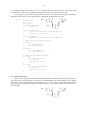
5. Iteration of IDEAL Constructs
5.1. Pens
In Donald Knuth’s METAFONT system, pens are different shapes—circles, ellipses, and
polygons—that draw along curves. IDEAL includes pens as a generalization of this idea: any box
may be used to draw along a line. For instance, users may define ‘‘dashed’’ or ‘‘dotted’’ pens. A
pen statement looks like this:
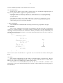
- 11 -
conn x to y
using n pen {
...
} <a,b>;
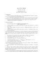
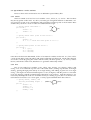
(The only keywords in this statement are conn, to, and using.) Pen may be any box. IDEAL will
place n copies of pen in the space from x to y. a and b are expressions known to pen. The first
instance of pen will have a at x, and the last instance of pen will have b at y; every instance in
between will have its a at the preceding one’s b, and its b at the succeeding one’s a, as shown in
this picture:
________________
________________________
________
x a
b a
b ... a
b a
b a
b ... a
b y
1
i–1 i
n
2
i+1
________________
________________________
________
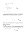
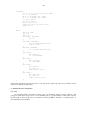
Here is an example box that contains an angular wavy path:
(start)
(end)
wavy {
var start, end, perp, pt1, pt2, ht;
perp = (0,1)*(start - end)/abs(start - end);
pt1 = 0.25[start,end] + perp*ht;
pt2 = 0.75[start,end] - perp*ht;
conn start to pt1 to pt2 to end;
}
Here we use wavy as a pen to indicate that part of a rectangle is missing.
_________
main {
var ne, nw, se, sw;
var n1, s1, n2, s2;
______ ______
ne = nw + 2;
se =
ne =
n2 s2 conn
conn
sw + 2;
se + (0,1);
0.4 = n1 = 0.6[nw,ne];
0.4 = s1 = 0.4[sw,se];
n1 to nw to sw to s1;
n1 to s1
using int(5*abs(n1-s1)) wavy {
ht = -0.1;
} <start,end>;
conn n2 to ne to se to s2;
conn n2 to s2
using int(5*abs(n2-s2)) wavy {
ht = -0.1;
} <start,end>;
}
We can change wavy to contain a smooth wave by changing the word conn in the fifth line of its
definition to spline, and use the same instructions above to draw the picture with the new pen.
- 12 -
_________
______ ______
5.2. Pens as For-Statements
The pen statement
conn x to y
using n pen {
...
} <a,b>;
has the same effect as
for i = 1 to n {
put pen {
a = ((i-1)/n)[x,y];
b = (i/n)[x,y];
...
};
}
imagining for a moment that IDEAL had for-statements.
This means a pen statement can be used to synthesize a for-statement in an
Here is a pen statement to draw a dashed arc:
IDEAL
program.
conn 0 to 180
using 10 arc {
center = 0;
radius = 1;
}<startang, 9+endang>;
To draw a set of concentric circles we can say:
main {
conn 1 to 6
using 5 circle {
center = 0;
} <radius,radius+1>;
}
In the first example, the second expression in angle brackets is important: it means that each
‘‘dash’’ covers nine degrees. In the second example, this expression is redundant: its only purpose is to prevent IDEAL from generating a stream of error messages about inconsistent equations. This contorted way of simulating for-statements is necessary only because pens are
meant to do the right thing at each end of and all along a path that is being drawn with some
box, and not as general iteration constructs.
Why doesn’t IDEAL have for-statements? Notice that every variable in an IDEAL program is
assigned a value exactly once. Obviously the index of a for-statement must be an exception to
that rule. Generating the index internally prevents the need to have two kinds of variables—
changing and fixed. The local variables of boxes placed by pen statements cannot be referenced
outside the pen statement, because the boxes are not named when they are placed. A general
for-statement could lead to the need to generate automatically names for different instances of
boxes, a hard problem that I don’t understand well enough yet.
- 13 -
5.3. Filling Regions
Because any box can be used as a pen, we can shade regions. (We can have not only dashed
and dotted ink, but checkered paint!) Take box wavy, for instance. First we construct a box brush,
which consists of seven copies of wavy going horizontally:
brush {
var top, bot;
var bwd, bht;
var leftpt, rightpt;
leftpt = 0.5*(top+bot) - bwd/2;
rightpt = 0.5*(top+bot) + bwd/2;
conn leftpt to rightpt
using 7 wavy {
ht = bht;
}<start,end>;
}
Then we use ‘‘brush’’ to draw vertically over the region of interest.
conn (0,1) to (0,-1)
using 6 brush {
bwd = 2;
bht = 0.1;
}<top,bot>;
6. Opaque Boxes
IDEAL includes statements to blot out pieces of a picture. In this section we will sometimes
place opaque boxes without explicitly drawing any background. In such cases, assume that we
have painted over the area with pens as above.
6.1. Opaque Polygons
IDEAL needs to know the vertices of a polygon in order to opaque the area it covers. The
vertices are specified as a list in a bdlist statement. For instance, to opaque a rectangular region
using the rect box defined in Section 3, we could use the following statement:
put rect {
opaque;
bdlist = sw, se, ne, nw;
sw = (-0.4,-0.4);
wd = ht = 1;
};
________
________
The sides of the rectangle are drawn by rect: they are not supplied automatically by the opaqueing routine. If we wanted to save only the interior of the rectangle, we could use almost the same
statement:
- 14 -
put rect {
opaque exterior;
bdlist = sw, se, ne, nw;
sw = (-0.4,-0.4);
wd = ht = 1;
};
________
________
If we plan to opaque a lot of rectangles, we should include a bdlist in the definition of rect.
Such a default bdlist would be referenced only if the parameter section of the put statement
included an opaque statement and did not include its own bdlist.
6.2. Opaque Circular Arc Polygons
The edges of opaque regions can also be circular arcs.
This generalization of the simple boundary statement is the most recent addition to IDEAL. It
avoids treating circles and their sectors and segments as special cases, and makes opaqueing
circular arc polygons much easier.
To specify a circular arc edge, one gives its endpoints and a point through which it passes; this
‘‘pass-through’’ point is marked in the boundary list by the symbol ‘‘ˆ’’. For example, the boundary list for the sector shown below is
boundary = center, cis(30), ˆ cis(45), cis(60);
Another common opaque arc is the segment:
boundary = cis(0), ˆ cis(45), cis(90);
One can construct an opaque circle out of two semicircular edges:
boundary = cis(0), ˆ cis(90), cis(180), ˆ cis(270);
Here, the outer circle has an opaque exterior, while the inner circle has an opaque interior.
6.3. Order is Important
Without the ability to opaque, the order in which boxes are put does not matter. But when
some boxes are opaque, order obviously does matter. Put statements are executed in the order in
which they appear in the box definition. When an opaque box is drawn, the opaquing is done
first, then the lines of the box are drawn; so, for instance, an opaque listnode does include the line
- 15 -
down its middle separating its info field from its next field.
6.4. Some Hard Facts
Neither text nor splines can be used to opaque objects, nor will they be clipped properly if
they are in a picture and an opaque box is placed over them.
The problem with text is that IDEAL operates as a TROFF preprocessor, so it cannot determine
anything about the size of the text, and it needs to know that if it is to do anything involving
opaquing and text.
The problem with splines is more subtle. When a line or circular arc is chopped, it is easy to
specify the lines or circular arcs that remain. But when a spline is chopped, the guiding points
of the resulting curve pieces are hard to determine.
7. Paper Commands
IDEAL
includes two commands that are analogous to the way people draw on paper.
7.1. Construct
The construct statement looks just like a put statement, with the keyword put replaced by
construct. It is best to think of it as laying a sheet of tracing paper over the current drawing.
Anything constructed will be drawn on this sheet. When you return to the layer underneath, you
may refer to any of the local variables as with a put statement, but the lines and curves in the constructed picture don’t show.
main {
construct A: rect
sw = 0;
wd = ht =
};
construct B: rect
n = A.s wd = ht =
};
’top’ at A.c;
’bottom’ at B.c;
put arrow {
hd = B.n;
tl = A.s;
};
{
1;
{
(0,1);
1;
top
bottom
}
Here we have used ‘‘invisible boxes’’ to place the arrow around the text without drawing the
boxes.
7.2. Draw
The construct command may also be used to localize the effects of opaque boxes. We saw
above how to draw a filled polygon: paint over the area, then opaque the exterior of the polygon.
But how can we draw two filled polygons in the same picture?
One solution is to construct them both, then use the draw command to add them to the
main picture. The draw command transfers the contents of the named sheet of tracing paper to
the sheet below.
- 16 -
null {
}
pentagon {
var center, radius,
pt1, pt2, pt3, pt4, pt5;
_________
pt1 = center + radius;
pt2 = center + cis(72)*radius;
pt3 = center + cis(144)*radius;
pt4 = center + cis(-144)*radius;
pt5 = center + cis(-72)*radius;
conn pt1 to pt2 to pt3 to pt4 to pt5 to pt1;
bdlist = pt1, pt2, pt3, pt4, pt5;
}
main {
construct A: null {
conn (0,1) to 0
using 7 brush {
bwd = 1;
bht = 0.1;
}<top,bot>;
put pentagon {
center = (0,0.5);
radius = (0,0.5);
opaque exterior;
};
};
construct B: null {
conn (0.5,0.5) to (1.5,0.5)
using 5 brush {
bwd = (0,1);
bht = 0.1;
}<top,bot>;
put circle {
center = (1,0.5);
radius = 0.5;
opaque exterior;
};
};
draw A;
draw B;
}
Even put statements can be added to the parameter sections of construct (and put) statements!
Believe it or not, box null defined above is one of the most useful: it gives us a way to name a set
of commands and variables so that we may reference them later, yet it doesn’t require us to
define a box that will be used only once.
Given construct and draw, why do we need a special box hole to opaque a circular area
without drawing anything? Why not just construct an opaque circle, then draw it on the main
picture? The problem is that the effect of opaquing is localized just as much as the drawing, so an
opaque constructed circle won’t opaque anything that lies underneath.
- 17 -
8. Library Files
Library files are available to draw common figures and for special figures like circles and
arcs. To include a library file as part of an IDEAL program, include the line
...libfile name
in your IDEAL program (between the .IS and .IE lines that mark its start and end.) This section
describes available library files that have been alluded to up to now.
8.1. Rectangle
File rect contains the definition of box rect, which looks like the definition in Section 3, with
five more variables: n, s, e, w, and c, which are the four compass points and the center, respectively.
rect {
var ne, nw, sw, se,
n, e, w, s, c,
ht, wd;
ne = se + (0,1)*ht;
nw = sw + (0,1)*ht;
ne = nw + wd;
n = (ne+nw)/2;
s = (se+sw)/2;
e = (ne+se)/2;
w = (nw+sw)/2;
c = (ne+sw)/2;
ht ˜ 1;
wd ˜ 1.5;
bdlist = ne, nw, sw, se;
conn ne to nw to sw to se to ne;
}
8.2. Arrow
File arrow contains the definition of box arrow as given in Section 3.
arrow {
var tl, hd, head, perp, headang;
conn tl to hd;
perp = head*(tl-hd)/abs(tl-hd);
conn hd + cis(headang)*perp to hd to hd + cis(-headang)*perp;
head ˜ 0.1;
headang ˜ 25;
}
8.3. Wavy
Library file wavy contains the definition for the familiar wavy.
wavy {
var start, end, perp, pt1, pt2, ht;
perp = (0,1)*(start - end)/abs(start - end);
pt1 = 0.25[start,end] + perp*ht;
pt2 = 0.75[start,end] - perp*ht;
conn start to pt1 to pt2 to end;
}
- 18 -
8.4. Dash
Library file dash contains the definition of box dash, which may be useful for drawing
dashed lines:
dash {
var start, end;
conn start to 0.25[start,end];
conn 0.75[start,end] to end;
}
8.5. Circles
Box circle resides in a library file of the same name, and has the local variables described in
Section 3: center, radius, z1, z2, and z3.
Box circle actually consists of variable declarations and a put of box CIRCLE. So, if you will
have many circles of a particular radius, it might be easier for you to define your own, say, circle3:
circle {
var center, radius, z1, z2, z3;
put CIRCLE {
radius = 3;
}
}
8.6. Arcs
Box arc is contained in a library file of the same name, with local variables as described in
Section 3: center, radius, start, midway, end, startang, midang, and endang.
As above, arc calls on a box called ARC.
9. Examples
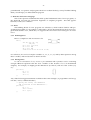
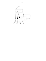
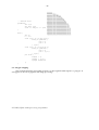
9.1. B-Trees
This example depicts a B-tree whose nodes have many children.*
__________________
*P. J. Weinberger, Unix B-trees, Bell Laboratories, 1981.
- 19 -
__________________
.
.
.
.
__________________
__________________
•
•
__________________
•
__________________
___________
__________________
•
•
______ •
______
__________________
- 20 -
...libfile rect
arrow {
var tl,
headvec
conn tl
conn hd
hd, headvec, head;
= hd + head*(tl - hd)/abs(tl - hd);
to hd;
+ cis(20)*(headvec - hd)
to hd
to hd + cis(-20)*(headvec - hd);
}
dot {
var s, e;
’\(bu’ at 0.5[s, e] - (0,0.1);
}
per {
var s, e;
’.’ at 0.5[s, e];
}
main {
var rw, rh;
rw = 2;
rh = 1;
var hmv, vmv;
hmv = 0.6;
vmv = 0.3;
var ah;
ah = 0.2;
put root: rect {
sw = (0,1);
wd = rw;
ht = 1;
};
put next: rect {
sw = youngest.sw + 2*(hmv, vmv);
wd = rw;
ht = rh;
};
put youngest: rect {
sw = bro.sw + (hmv, vmv);
wd = rw;
ht = rh;
opaque;
};
put bro: rect {
sw = eldest.sw + (hmv, vmv);
wd = rw;
ht = rh;
opaque;
};
put eldest: rect {
im(nw) = im(3[root.nw,root.sw]);
re(0.5[nw, next.nw]) = re(0.5[root.nw, root.ne]);
wd = rw;
ht = rh;
opaque;
put arrow {
head = ah;
- 21 -
tl = 0.0[sw, se] + 0.5 * (nw - sw);
hd = tl - (0, 1) * cis(-27);
};
put arrow {
head
tl =
hd =
};
put arrow {
head
tl =
hd =
};
put arrow {
head
tl =
hd =
};
= ah;
0.33[sw, se] + 0.5 * (nw -sw);
tl - (0,1) * cis(-9);
= ah;
0.67[sw, se] + 0.5 * (nw - sw);
tl - (0,1) * cis(9);
= ah;
1.0[sw, se] + 0.5 * (nw -sw);
tl - (0,1) * cis(27);
};
put arrow {
head = ah;
tl=root.sw + 0.5 * (root.nw - root.sw);
hd=eldest.nw;
};
put arrow {
head = ah;
tl=0.1[root.sw,root.se] + 0.5 * (root.nw - root.sw);
hd=bro.nw;
};
put a: arrow {
head = ah;
tl=0.2[root.sw,root.se] + 0.5 * (root.nw - root.sw);
hd=youngest.nw;
};
put b: arrow {
head = ah;
tl = 0.5[root.ne, root.se];
hd = next.nw;
};
put arrow {
head = ah;
hd = root.nw;
tl = 0.5[root.nw, root.ne] + (0, 1.0);
};
conn next.nw to youngest.nw using 3 dot{}<s, e>;
conn next.se to youngest.se using 3 dot{}<s, e>;
conn b.tl to a.tl using 4 per{}<s, e>;
}
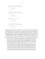
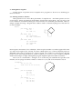
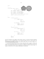
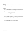
9.2. A Sector Grid
Norm Schryer used this figure to show how numerical integration is used to find the area of
planar regions.
- 22 -
_________
_____________
________________
__________________
____________________
_____________________
_ _____________________
________________________
...libfile hole
_________________________
gridline {
_ ________________________
__________________________
var a,b;
___________________________
var neg, pos;
___________________________
conn a - neg to a + pos; _
____________________________
___________________________
}
_____________________________
_____________________________
_____________________________
_____________________________
main {
_____________________________
var n;
n = 21;
conn (0,0) to (0,1+1/(n-1))
using n gridline {
neg = 0;
pos = 1;
} <a,b>;
conn (0,0) to (1+1/(n-1),0)
using n gridline {
neg = 0;
pos = (0,1);
} <a,b>;
put hole {
radius = 1;
center = (0,0);
opaque exterior;
};
}
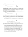
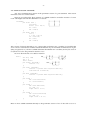
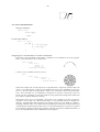
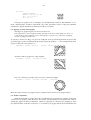
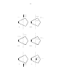
9.3. Polygon Clipping
This example illustrates all possible positions of a line segment with respect to a polygon. It
will appear in a book on graphics and image processing.*
__________________
*T. Pavlidis, Graphics and Image Processing, to be published.
- 23 -
P 2 (P 1 )
++−−
(a)
+−−+
(−++−)
(c)(c1)
−−++
P 1 (P 2 )
(b)(b1)
P 1 (P 2 )
P 2 (P 1 )
(d)(d1)
(f)
P 2 (P 1 )
P 1 (P 2 )
P 2 (P 1 )
P 1 (P 2 )
P 1 (P 2 )
(e)
P 1 (P 2 )
P 2 (P 1 )
P 2 (P 1 )
+−−−
(−+−−)
−−−+
(−−+−)
−−−−
- 24 -
.ps 8
.EQ
gsize 8
define P12 " P sub 1 ( P sub 2 ) "
define P21 " P sub 2 ( P sub 1 )"
.EN
...libfile circle
...minx -1
...maxx 6
...miny -1
...maxy 12
box spot{
var loc;
put circle{
var center, radius;
center = loc;
radius = 0.02;
opaque;
};
}
box vert{
var midd, llength;
conn midd+llength to midd-llength;
}
box poly{
var c1,p1,p2,p3,p4,p5,r1,tp,bp,ta,tb;
p1 = c1+r1;
p2 = cis(65)[c1,p1];
p3 = cis(170)[c1,p1];
p4 = cis(190)[c1,p1];
p5 = cis(300)[c1,p1];
tp = c1+(0,ta)*r1;
bp = c1+(0,tb)*r1;
conn p1 to p2;
conn p2 to p3;
conn p3 to p4;
conn p4 to p5;
conn p5 to p1;
put vert{ midd=c1; llength=(0,1.6)*r1; };
put spot{ loc=tp; };
put spot{ loc=bp; };
left ’$P12$’ at tp+0.1;
left ’$P21$’ at bp+0.1;
}
box main {
put poly{
c1 =(1,9); r1 = (1,0); ta=1.1; tb=1.4;
left ’$++--$’ at p2-1.5;
right ’(a)’ at c1-(0.7,1.2);
};
put poly{
c1 =(3.5,9); r1 = (1,0); ta=1.1; tb=0.2;
left ’$+---$’ at p2+0.5;
left ’$(-+--)$’ at p2+(0.5,-0.15);
right ’(b)(b1)’ at c1-(0.7,1.2);
};
put poly{
c1 =(1,5); r1 = (1,0); ta=1.1; tb=-1;
left ’$+--+$’ at p2-1.5;
- 25 -
left ’$(-++-)$’ at p2-(1.5,0.15);
right ’(c)(c1)’ at c1-(0.7,1.2);
};
put poly{
c1 =(3.5,5); r1 = (1,0); ta=0.2; tb=-1;
left ’$---+$’ at p2+(0.5,-0.3);
left ’$(--+-)$’ at p2+(0.5,-0.45);
right ’(d)(d1)’ at c1-(0.7,1.2);
};
put poly{
c1 =(1,1); r1 = (1,0); ta=-1; tb=-1.4;
left ’$--++$’ at p4-(0,0.5);
right ’(e)’ at c1-(0.7,1.2);
};
put poly{
c1 =(3.5,1); r1 = (1,0); ta=0.2; tb=-0.2;
left ’$----$’ at p1+0.2;
right ’(f)’ at c1-(0.7,1.2);
};
}
10. Acknowledgements
My thanks to all who read drafts of this manual and criticized constructively: Al Aho,
Lorinda Cherry, Eric Grosse, Steve Johnson, Brian Kernighan, John Mashey, Doug McIlroy, and
Theo Pavlidis; and to early users of IDEAL, especially Eric Grosse, Theo Pavlidis, Norm Schryer,
and Peter Weinberger.
2.
M. E. Lesk, Tbl—a program to format tables, Bell Laboratories, Murray Hill, New Jersey (1976).
3.
Joseph F. Ossanna, NROFF/TROFF User’s Manual, Bell Laboratories, Murray Hill, New Jersey
(1976).