1
LINFOR3D User Manual
version 5.1.4
Matthias Steffen
Hans-G¨
unter Ludwig
October 21, 2014
1
Sven Wedemeyer-B¨
ohm
2
CONTENTS
Contents
1 Introduction
6
2 Getting started
6
3 Basic Equations of Radiative Transfer
3.1 Transfer equation for the continuum intensity
3.2 Transfer equation for the line intensity . . . .
3.3 Transfer equation for the line depression . . .
3.4 Contribution functions . . . . . . . . . . . . .
3.5 Grey test case . . . . . . . . . . . . . . . . . .
4 Program Files and Data
4.1 Main program flow . .
4.2 Structures in Common
4.3 IDL Files . . . . . . .
.
.
.
.
.
7
7
8
9
10
12
input files
. . . . . . . . . . . . . . . . . . . . . . . . . . . . . . . . . .
Block linfordata . . . . . . . . . . . . . . . . . . . . . . . .
. . . . . . . . . . . . . . . . . . . . . . . . . . . . . . . . . .
17
17
18
18
5 Parameter Input: linfor setcmd.pro
5.1 Program execution flags . . . . . . . .
5.1.1 run flag . . . . . . . . . . . . .
5.1.2 cv1 flag . . . . . . . . . . . . .
5.1.3 cv2 flag . . . . . . . . . . . . .
5.1.4 cv3 flag . . . . . . . . . . . . .
5.1.5 plt flag . . . . . . . . . . . . .
5.1.6 maps flag . . . . . . . . . . . .
5.1.7 cc3d flag . . . . . . . . . . . . .
5.1.8 nlte flag . . . . . . . . . . . . .
5.1.9 free flag . . . . . . . . . . . . .
5.2 General paths . . . . . . . . . . . . . .
5.2.1 abupath . . . . . . . . . . . . .
5.2.2 ff path . . . . . . . . . . . . . .
5.2.3 opapath . . . . . . . . . . . . .
5.2.4 gaspath . . . . . . . . . . . . .
5.2.5 eospath . . . . . . . . . . . . .
5.3 Model data . . . . . . . . . . . . . . .
5.3.1 context . . . . . . . . . . . . .
5.3.2 rhdpath . . . . . . . . . . . . .
5.3.3 modelid . . . . . . . . . . . . .
5.3.4 parfs . . . . . . . . . . . . . . .
5.3.5 xbcpath . . . . . . . . . . . . .
5.3.6 abuid . . . . . . . . . . . . . .
5.3.7 dmetal . . . . . . . . . . . . . .
5.3.8 dalpha . . . . . . . . . . . . . .
5.3.9 nx skip . . . . . . . . . . . . .
5.3.10 ny skip . . . . . . . . . . . . .
5.4 More model information (all read from
5.4.1 opafile . . . . . . . . . . . . . .
5.4.2 gasfile . . . . . . . . . . . . . .
5.4.3 eosfile . . . . . . . . . . . . . .
5.4.4 htau0 . . . . . . . . . . . . . .
5.4.5 qmol . . . . . . . . . . . . . . .
5.4.6 Teff . . . . . . . . . . . . . . .
.
.
.
.
.
.
.
.
.
.
. . . . . .
. . . . . .
. . . . . .
. . . . . .
. . . . . .
. . . . . .
. . . . . .
. . . . . .
. . . . . .
. . . . . .
. . . . . .
. . . . . .
. . . . . .
. . . . . .
. . . . . .
. . . . . .
. . . . . .
. . . . . .
. . . . . .
. . . . . .
. . . . . .
. . . . . .
. . . . . .
. . . . . .
. . . . . .
. . . . . .
. . . . . .
parameter
. . . . . .
. . . . . .
. . . . . .
. . . . . .
. . . . . .
. . . . . .
.
.
.
.
.
.
.
.
.
.
.
.
.
.
.
.
.
.
.
.
.
.
.
.
.
.
.
.
.
.
.
.
.
.
.
.
.
.
.
.
.
.
.
.
.
.
.
.
.
.
.
.
.
.
.
.
.
.
.
.
.
.
.
.
.
.
.
.
.
.
. . . . . . . . . . . . . .
. . . . . . . . . . . . . .
. . . . . . . . . . . . . .
. . . . . . . . . . . . . .
. . . . . . . . . . . . . .
. . . . . . . . . . . . . .
. . . . . . . . . . . . . .
. . . . . . . . . . . . . .
. . . . . . . . . . . . . .
. . . . . . . . . . . . . .
. . . . . . . . . . . . . .
. . . . . . . . . . . . . .
. . . . . . . . . . . . . .
. . . . . . . . . . . . . .
. . . . . . . . . . . . . .
. . . . . . . . . . . . . .
. . . . . . . . . . . . . .
. . . . . . . . . . . . . .
. . . . . . . . . . . . . .
. . . . . . . . . . . . . .
. . . . . . . . . . . . . .
. . . . . . . . . . . . . .
. . . . . . . . . . . . . .
. . . . . . . . . . . . . .
. . . . . . . . . . . . . .
. . . . . . . . . . . . . .
. . . . . . . . . . . . . .
file for CO5 BOLD data)
. . . . . . . . . . . . . .
. . . . . . . . . . . . . .
. . . . . . . . . . . . . .
. . . . . . . . . . . . . .
. . . . . . . . . . . . . .
. . . . . . . . . . . . . .
.
.
.
.
.
.
.
.
.
.
.
.
.
.
.
.
.
.
.
.
.
.
.
.
.
.
.
.
.
.
.
.
.
.
.
.
.
.
.
.
.
.
.
.
.
.
.
.
.
.
.
.
.
.
.
.
.
.
.
.
.
.
.
.
.
.
.
.
.
.
.
.
.
.
.
.
.
.
.
.
.
.
.
.
.
.
.
.
.
.
.
.
.
.
.
.
.
.
.
.
.
.
.
.
.
.
.
.
.
.
.
.
.
.
.
.
.
.
.
.
.
.
.
.
.
.
.
.
.
.
.
.
.
.
.
.
.
.
.
.
.
.
.
.
.
.
.
.
.
.
.
.
.
.
.
.
.
.
.
.
.
.
.
.
.
.
.
.
.
.
.
.
.
.
.
.
.
.
.
.
.
.
.
.
.
.
.
.
.
.
20
20
20
21
21
21
21
22
22
22
23
23
23
23
24
24
24
24
24
24
25
25
25
25
25
26
26
26
26
26
27
27
27
27
27
CONTENTS
.
.
.
.
.
.
.
.
.
.
.
.
.
.
.
.
.
.
.
.
.
.
.
.
.
.
.
.
.
.
.
.
.
.
.
.
.
.
.
.
.
.
.
.
.
.
.
.
.
.
.
.
.
.
.
.
.
.
.
.
.
.
.
.
.
.
.
.
.
.
.
.
.
.
.
.
.
.
.
.
.
.
.
.
.
.
.
.
.
.
.
.
.
.
.
.
.
.
.
.
.
.
.
.
.
.
.
.
.
.
.
.
.
.
.
.
.
.
.
.
.
.
.
.
.
.
.
.
.
.
.
.
.
.
.
.
.
.
.
.
.
.
.
.
.
.
.
.
.
.
.
.
.
.
.
.
.
.
.
.
.
.
.
.
.
.
.
.
.
.
.
.
.
.
.
.
.
.
.
.
.
.
.
.
.
.
.
.
.
.
.
.
.
.
.
.
.
.
.
.
.
.
.
.
.
.
.
.
.
.
.
.
.
.
.
.
.
.
.
.
.
.
.
.
.
.
.
.
.
.
.
.
.
.
.
.
.
.
.
.
.
.
.
.
.
.
.
.
.
.
.
.
.
.
.
.
.
.
.
.
.
.
.
.
.
.
.
.
.
.
.
.
.
.
.
.
.
.
.
.
.
.
.
.
.
.
.
.
.
.
.
.
.
.
.
.
.
.
.
.
.
.
.
.
.
.
.
.
.
.
.
.
.
.
.
.
.
.
.
.
.
.
.
.
.
.
.
.
.
.
.
.
.
.
.
.
.
.
.
.
.
.
.
.
.
.
.
.
.
.
.
.
.
.
.
.
.
.
.
.
.
.
.
.
.
.
.
.
.
.
.
.
.
.
.
.
.
.
27
27
28
28
28
28
29
29
29
29
29
29
29
30
30
30
30
30
30
30
31
31
31
31
32
32
32
32
33
33
33
33
33
33
34
34
34
34
34
35
35
36
6 Line Data File: line.dat
6.1 Parameters in Line Data File . . . . . . . . . . . . . . . . . . . . . .
6.1.1 clam . . . . . . . . . . . . . . . . . . . . . . . . . . . . . . . .
6.1.2 gfscale . . . . . . . . . . . . . . . . . . . . . . . . . . . . . . .
6.2 Line Data Formats . . . . . . . . . . . . . . . . . . . . . . . . . . . .
6.2.1 Continuum only . . . . . . . . . . . . . . . . . . . . . . . .
6.2.2 Single line calculations, line data format ‘0’ . . . . . .
6.2.3 Single line calculations, line data format ‘1’ . . . . . .
6.2.4 Single line calculations, complete line data format ‘2’
.
.
.
.
.
.
.
.
.
.
.
.
.
.
.
.
.
.
.
.
.
.
.
.
.
.
.
.
.
.
.
.
.
.
.
.
.
.
.
.
.
.
.
.
.
.
.
.
.
.
.
.
.
.
.
.
.
.
.
.
.
.
.
.
38
38
38
38
38
38
39
40
42
5.5
5.6
5.7
5.8
5.9
5.4.7 grav . . . . . . . . . . . .
5.4.8 tsurffac . . . . . . . . . .
Model data - reading of ’full’ files
5.5.1 isnap full 1 . . . . . . . .
5.5.2 isnap full 2 . . . . . . . .
5.5.3 istep full . . . . . . . . . .
h3Di mean model . . . . . . . . .
5.6.1 mavg . . . . . . . . . . .
External 1D reference model . .
5.7.1 atmpath . . . . . . . . . .
5.7.2 atmfile . . . . . . . . . . .
Line data and radiative transfer .
5.8.1 linfs . . . . . . . . . . . .
5.8.2 lutau1 . . . . . . . . . . .
5.8.3 lutau2 . . . . . . . . . . .
5.8.4 dlutau . . . . . . . . . . .
5.8.5 lctau1 . . . . . . . . . . .
5.8.6 lctau2 . . . . . . . . . . .
5.8.7 dlctau . . . . . . . . . . .
5.8.8 ntheta . . . . . . . . . . .
5.8.9 nphi . . . . . . . . . . . .
5.8.10 mu0 . . . . . . . . . . . .
5.8.11 kphi . . . . . . . . . . . .
5.8.12 Hbrd . . . . . . . . . . . .
5.8.13 ximicx . . . . . . . . . . .
5.8.14 ximic1 . . . . . . . . . . .
5.8.15 ximic3 . . . . . . . . . . .
5.8.16 ximacx . . . . . . . . . .
5.8.17 ximac1 . . . . . . . . . . .
5.8.18 ximac3 . . . . . . . . . . .
5.8.19 vfacx . . . . . . . . . . . .
5.8.20 vfacy . . . . . . . . . . . .
5.8.21 vfacz . . . . . . . . . . . .
5.8.22 micro . . . . . . . . . . .
5.8.23 xi a . . . . . . . . . . . .
5.8.24 xi b . . . . . . . . . . . .
5.8.25 xi d . . . . . . . . . . . .
5.8.26 dclam . . . . . . . . . . .
5.8.27 intmode . . . . . . . . . .
5.8.28 intline . . . . . . . . . . .
5.8.29 nchunk . . . . . . . . . .
Example . . . . . . . . . . . . . .
3
. . . . . . . . . .
. . . . . . . . . .
(CO5 BOLD only)
. . . . . . . . . .
. . . . . . . . . .
. . . . . . . . . .
. . . . . . . . . .
. . . . . . . . . .
. . . . . . . . . .
. . . . . . . . . .
. . . . . . . . . .
. . . . . . . . . .
. . . . . . . . . .
. . . . . . . . . .
. . . . . . . . . .
. . . . . . . . . .
. . . . . . . . . .
. . . . . . . . . .
. . . . . . . . . .
. . . . . . . . . .
. . . . . . . . . .
. . . . . . . . . .
. . . . . . . . . .
. . . . . . . . . .
. . . . . . . . . .
. . . . . . . . . .
. . . . . . . . . .
. . . . . . . . . .
. . . . . . . . . .
. . . . . . . . . .
. . . . . . . . . .
. . . . . . . . . .
. . . . . . . . . .
. . . . . . . . . .
. . . . . . . . . .
. . . . . . . . . .
. . . . . . . . . .
. . . . . . . . . .
. . . . . . . . . .
. . . . . . . . . .
. . . . . . . . . .
. . . . . . . . . .
.
.
.
.
.
.
.
.
.
.
.
.
.
.
.
.
.
.
.
.
.
.
.
.
.
.
.
.
.
.
.
.
.
.
.
.
.
.
.
.
.
.
.
.
.
.
.
.
.
.
.
.
.
.
.
.
.
.
.
.
.
.
.
.
.
.
.
.
.
.
.
.
.
.
.
.
.
.
.
.
.
.
.
.
.
.
.
.
.
.
.
.
.
.
.
.
.
.
.
.
.
.
.
.
.
.
.
.
.
.
.
.
.
.
.
.
.
.
.
.
.
.
.
.
.
.
.
.
.
.
.
.
.
.
.
.
.
.
.
.
.
.
.
.
.
.
.
.
.
.
.
.
.
.
.
.
.
.
.
.
.
.
.
.
.
.
.
.
.
.
.
.
.
.
.
.
.
.
.
.
.
.
.
.
.
.
.
.
.
.
.
.
.
.
.
.
.
.
.
.
.
.
.
.
.
.
.
.
.
.
.
.
.
.
.
.
.
.
.
.
.
.
.
.
.
.
.
.
.
.
.
.
.
.
.
.
.
.
.
.
.
.
.
.
.
.
.
.
.
.
.
.
.
.
.
.
.
.
.
.
.
.
.
.
.
.
.
.
.
.
.
.
.
.
.
.
.
.
.
.
.
.
.
.
.
.
.
.
.
.
.
.
.
.
.
.
.
.
.
.
.
.
.
.
.
.
.
.
.
.
.
.
.
.
.
.
.
.
.
.
.
.
.
.
.
.
.
.
.
.
.
.
.
.
.
.
.
.
.
.
.
.
.
.
.
.
.
.
.
.
.
.
.
.
.
.
.
.
.
.
.
.
.
.
.
.
.
.
.
.
.
.
.
.
.
.
.
.
4
CONTENTS
6.3
6.2.5 Single line calculations, complete line data format ‘3’
6.2.6 Single line calculations, complete line data format ‘7’
6.2.7 Multiple Line Calculations . . . . . . . . . . . . . . . . .
Conversion of line broadening parameters . . . . . . . . . . . .
6.3.1 Quadratic Stark effect . . . . . . . . . . . . . . . . . . . . . .
6.3.2 Van der Waals broadening . . . . . . . . . . . . . . . . . . .
6.3.3 Natural line broadening . . . . . . . . . . . . . . . . . . . . .
.
.
.
.
.
.
.
.
.
.
.
.
.
.
.
.
.
.
.
.
.
.
.
.
.
.
.
.
.
.
.
.
.
.
.
.
.
.
.
.
.
.
.
.
.
.
.
.
.
.
.
.
.
.
.
.
43
44
44
45
45
46
47
7 Output files
48
7.1 Files containing intensity maps . . . . . . . . . . . . . . . . . . . . . . . . . . . . . 48
7.2 Foreshortening . . . . . . . . . . . . . . . . . . . . . . . . . . . . . . . . . . . . . . 49
8 Timing statistics
9 IONDIS
9.1 Molecules . . . . . . . . . . . . .
9.1.1 Some definitions . . . . .
9.1.2 Equations . . . . . . . . .
9.1.3 Criterion for convergence
9.1.4 Initial guess . . . . . . . .
9.1.5 Variable names . . . . . .
50
.
.
.
.
.
.
.
.
.
.
.
.
.
.
.
.
.
.
.
.
.
.
.
.
.
.
.
.
.
.
.
.
.
.
.
.
.
.
.
.
.
.
.
.
.
.
.
.
.
.
.
.
.
.
.
.
.
.
.
.
.
.
.
.
.
.
.
.
.
.
.
.
.
.
.
.
.
.
.
.
.
.
.
.
.
.
.
.
.
.
.
.
.
.
.
.
.
.
.
.
.
.
.
.
.
.
.
.
.
.
.
.
.
.
.
.
.
.
.
.
.
.
.
.
.
.
.
.
.
.
.
.
.
.
.
.
.
.
.
.
.
.
.
.
.
.
.
.
.
.
.
.
.
.
.
.
.
.
.
.
.
.
.
.
.
.
.
.
51
51
51
51
54
54
55
LIST OF FIGURES
5
List of Figures
1
Analytical curve-of-growth . . . . . . . . . . . . . . . . . . . . . . . . . . . . . . . . 14
List of Tables
1
2
3
4
5
List of all structures in common blocks ’linfordata’
List of additional IDL modules . . . . . . . . . . .
List of all IDL modules . . . . . . . . . . . . . . .
Small molecular network: 5 atoms, 8 molecules . .
Large molecular network:10 atoms, 14 molecules .
.
.
.
.
.
.
.
.
.
.
.
.
.
.
.
.
.
.
.
.
.
.
.
.
.
.
.
.
.
.
.
.
.
.
.
.
.
.
.
.
.
.
.
.
.
.
.
.
.
.
.
.
.
.
.
.
.
.
.
.
.
.
.
.
.
.
.
.
.
.
.
.
.
.
.
.
.
.
.
.
.
.
.
.
.
.
.
.
.
.
18
18
19
51
51
6
1
2
GETTING STARTED
Introduction
LINFOR3D is based on the old code LINFOR. The present version of LINFOR3D is still preliminary.
The aim is to develop the code in IDL and to transform it to FORTRAN for better execution
efficiency, after it is checked and found to work properly under IDL.
Hence, users should be aware of the following limitations:
• Geometry: This version is limited to spectrum synthesis from local hydrodynamical
models (solar-type convective atmospheres). In a future version, it should be possible to
compute the line formation in global giant models.
• Efficiency: No effort was yet taken to really improve the execution speed of this
IDL/FORTRAN code. In fact there are still some parts in the code which are unnecessary for the current operation. Their execution should be controlled by additional flags in
a future release.
Like the code itself this user manual is under construction, too. Nevertheless, it will be of
substantial help while creating new command and spectral line data files for LINFOR3D.
To get a brief overview you might want to look into the section “Getting started” (Sect. 2) first.
2
Getting started
First make sure that you have all files which are listed in Tab. 3 and 2. These files should be put
together in a directory which can be accessed under IDL.
Now two files have to be edited and provided in order to run LINFOR3D:
• linforset_cmd.pro:
This file, which is an IDL script, defines the data structure cmd. This structure contains all
necessary information (except for spectral line data) like, e.g., paths and names of model
file(s). See Sect. 5 for more details.
• line.dat: This file contains all data for spectral line such as, e.g., oscillator strength and
broadening parameters. The usual file name is line.dat but it might be given another
name which then has be to entered in linfor_setcmd.pro. See Sect. 6 for more details.
After done so, you might start IDL and start LINFOR3D by simply typing
IDL> .r linfor_3D.pro
Several output files are created. It is also possible to directly use the results under IDL. See
Sect. 7 for more details.
Note that LINFOR3D stores the flow field in temporary cache files which are automatically restored
if the same calculation is repeated!
7
3
Basic Equations of Radiative Transfer
3.1
Transfer equation for the continuum intensity
d Iλc
= −κcλ Iλc + κcλ Sλc
ds
together with the definition of the optical depth along the ray
reads
(1)
d τλc = −κcλ d s ,
(2)
d Iλc
= Iλc − Sλc .
d τλc
(3)
The solution of Eq. (3) is
Iλc (τλc ) =
Z τb
λ
τλc
Sλc (τ 0 ) exp{−(τ 0 − τλc )} d τ 0 + Iλc (τλb ) exp{−(τλb − τλc )}
(4)
where τλb is the continuum optical depth at the lower boundary. The emergent continuum
intensity is:
Iλc (τλc
= 0) =
Z τb
λ
0
Sλc (τ 0 ) exp{−τ 0 } d τ 0 + Iλc (τλb ) exp{−τλb } .
(5)
Defining
we have the transport equation
ucλ = Iλc − Sλc
(6)
d Sλc
d ucλ
c
=
u
−
.
λ
d τλc
d τλc
(7)
The solution for ucλ is found by replacing Sλc by d Sλc /d τλc in Eq.(4):
ucλ (τλc )
=
Z τb
c 0
λ d S (τ )
λ
d τλc
τλc
exp{−(τ 0 − τλc )} d τ 0 + ucλ (τλb ) exp{−(τλb − τλc )}
(8)
The emergent intensity can also be obtained from Eq.(8):
Iλc (τλc
= 0) =
Sλc (τλc
Z τb
c 0
λ d S (τ )
λ
= 0) +
exp{−τ 0 } d τ 0 + ucλ (τλb ) exp{−τλb } .
c
0
d τλ
(9)
Now we define a fixed central wavelength, λ0 , with the corresponding fixed (universal) optical
depth scale τ0 , which is equidistant in log τ0 and may used alternatively for all integrations. On
this optical depth scale, Eq.(4) becomes
Iλc (τ0 )
Z τb c
0 κ
c 0
c
0
c b
c b
c
λ c 0
S
(τ
)
exp{−
τ
(τ
)
−
τ
(τ
)
}
d
τ
+
I
(τ
)
exp{−
τ
(τ
)
−
τ
(τ
)
} , (10)
=
0
0
λ
0
λ
0
λ
0
λ
0
λ
0
λ
c
τ0
κ0
giving the continuum intensity at wavelength λ as a function of optical depth τ0 . Note the factor
κcλ /κc0 under the integral. The intensity at the lower boundary, Iλc (τ0b ), can be computed from
the diffusion approximation,
Iλc (τ0b ) = Sλc (τ0b ) +
κc0 d Sλc b
(τ ) ,
κcλ d τ0 0
(11)
but the boundary term may also be neglected, at least for the emergent intensity, because the
exponential factor is usually very small. For the emergent intensity we have from Eq.(5):
Iλc (τ0
= 0) =
Z τb c
0 κ
λ
0
κc0
Sλc (τ00 ) exp{−τλc (τ00 )} d τ00 + Iλc (τ0b ) exp{−τλc (τ0b )} .
(12)
8
3
BASIC EQUATIONS OF RADIATIVE TRANSFER
Similarly, Eq.(8) becomes
ucλ (τ0 )
Z τb
c
0 dS
λ 0
=
(τ0 ) exp{−τλc (τ00 ) − τλc (τ0 )} d τ00 + ucλ (τ0b ) exp{−τλc (τ0b ) − τλc (τ0 )} .
τ0
d τ0
(13)
Note the absence of the factor κcλ /κc0 under the integral in this case. ucλ (τ0b ) is obtained from the
diffusion approximation,
κc d Sλc b
(τ ).
(14)
ucλ (τ0b ) = c0
κλ d τ0 0
The emergent intensity can be computed from Eq.(13) as:
Iλc (τ0
= 0) =
Sλc (τ0
Z τb
c
0 dS
λ 0
= 0) +
(τ0 ) exp{−τλc (τ00 )} d τ00 + ucλ (τ0b ) exp{−τλc (τ0b )} .
d τ0
0
(15)
In the latest version of Linfor3D, the continuum intensity is calculated from Eqs.(8) and (9), at 3
different wavelengths: λ0 − ∆λ, λ0 , and λ0 + ∆λ, where ∆λ is specified by the parameter dclam.
We ensure that the derivative d Sλc /d τ0 fulfills the condition
Z τ2
d Sλc
τ1
d τλ
(τλ0 ) d τλ0 = Sλc (τ2 ) − Sλc (τ1 ) .
(16)
The reason for using Eqs.(8) and (9) instead of Eq.(5) is that the quantity ucλ (τ ) is needed to
compute the line depression source function (see Sect. 3.3). We have checked that the usual transfer equation, Eq.(5), gives numerically very closely the same results for the emergent continuum
intensity as Eq.(9).
3.2
Transfer equation for the line intensity
In the presence of lines, the transfer equation at wavelength λ reads
X
d Iλ`
= − κcλ +
κ`λ
ds
`
!
Iλ` + κcλ Sλc +
X
κ`λ Sλ` .
(17)
`
The line source functions Sλ` may be different from the LTE continuum source function Sλc . With
the definition of the total optical depth
!
d τλ = −
κcλ
X
+
κ`λ
d s ≡ d τλc + d τλ` ,
(18)
`
and the total source function
Sλc + η Sλ`
κc S c
κ`λ Sλ`
1+β c
Sλ = c λPλ ` + c ` P
=
=
S ,
`
1+η
1+η λ
κλ + ` κλ κλ + ` κλ
P
where
` `
` κλ Sλ
Sλ` = P
,
`
` κλ
P
we can write
`
` κλ
c
κλ
P
η=
` `
` κλ Sλ
c
κλ Sλc
(19)
P
,
β=
,
d Iλ`
= Iλ` − Sλ .
d τλ
(20)
(21)
In LTE, Sλ = Sλc . The solution of Eq.(21) is
Iλ` (τλ = 0) =
Z τb
λ
0
Sλ (τλ0 ) exp{−τλ0 } d τλ0 + Iλ` (τλb ) exp{−τλb } .
(22)
3.3
Transfer equation for the line depression
9
In analogy to Eq.(12), we can also obtain the emergent line intensity by integration on the
universal optical depth scale τ0 :
Iλ` (τ0 = 0) =
Z τb c
0 κ
λ
0
κc0
(1 + η) Sλ (τ00 ) exp{−τλ (τ00 )} d τ00 + Iλ` (τ0b ) exp{−τλ (τ0b )} ,
(23)
or, substituting Sλ from Eq.(19),
Iλ` (τ0 = 0) =
Z τb c
0 κ
λ
0
κc0
(1 + β) Sλc (τ00 ) exp{−τλ (τ00 )} d τ00 + Iλ` (τ0b ) exp{−τλ (τ0b )} .
(24)
Integration on the log τ0 scale (z0 ≡ log τ0 ) gives:
Iλ` (z0a ) =
Z zb
0
z0a
ln(10) τ0 (z00 )
κcλ
(1 + β) Sλc (z00 ) exp{−τλ (z00 )} d z00 + Iλ` (z0b ) exp{−τλ (z0b )} ,
κc0
(25)
where z0a is the minimum log optical depth. Alternatively, in analogy to Eq.(9) we obtain:
Iλ` (τλ = 0) = Sλ (τλ = 0) +
Z τb
λ d Sλ
d τλ
0
(τλ0 ) exp{−τλ0 } d τλ0 + u`λ (τλb ) exp{−τλb } ,
(26)
where we have defined
u`λ = Iλ` − Sλ ,
(27)
which in the diffusion approximation may be written as
u`λ (τλb ) =
d Sλ b
(τ )
d τλ λ
κc0 /κcλ d Sλ b
(τ ).
1 + η d τ0 0
or u`λ (τ0b ) =
(28)
On the universal optical depth scale τ0 we obtain from Eq.(26:
Iλ` (τ0
= 0) = Sλ (τ0 = 0) +
Z τb
0 d Sλ
0
d τ0
(τ00 ) exp{−τλ (τ00 )} d τ00 + u`λ (τ0b ) exp{−τλ (τ0b )} ,
(29)
In LTE, where Sλ = Sλc , the integral in Eq.(29) differs from the integral in Eq.(15) only by the
exponential factor which involves the total optical depth τλ instead of the continuum optical
depth τλc . The absolute line depression is then calculated as
Dλ = Iλc (τ = 0) − Iλ` (τ = 0) .
(30)
In the current version of Linfor3D, Eq.(25) is used if the parameter intline is set to −1, and
Eq.(26) is used if intline is set to −2.
3.3
Transfer equation for the line depression
We may analyse the transfer equation for the absolute line depression defined in Eq.(30):
X
d Dλ
d Iλc
d I`
=
− λ = −κcλ Iλc + κcλ +
κ`λ
ds
ds
ds
`
or
X
d Dλ
= − κcλ +
κ`λ
ds
`
or
!
Iλ` −
X
κ`λ Sλ`
(31)
`
!
!
Dλ +
Iλc
X
`
d Dλ
= Dλ − SλD ,
d τλ
κ`λ
−
X
κ`λ Sλ`
(32)
`
(33)
10
3
BASIC EQUATIONS OF RADIATIVE TRANSFER
where the line depression source function is
SλD =
η c
η c
Iλ − Sλ` =
(Iλ − Sλc ) + (Sλc − Sλ` ) .
1+η
1+η
(34)
η
(I c − Sλc ) .
1+η λ
(35)
In LTE, Sλ` = Sλc , and
SλD =
The solution of Eq.(33) is
Dλ (τλ = 0) =
Z τb
λ
0
SλD (τλ0 ) exp{−τλ0 } d τλ0 ,
(36)
neglecting the boundary term. Integration on the fixed τ0 scale:
Dλ (τ0 = 0) =
Z τb c
0 κ
λ
κc0
0
(1 + η) SλD (τ00 ) exp{−τλ (τ00 )} d τ00 .
(37)
Substituting SλD from Eq.(34) gives
Dλ (τ0 = 0) =
Z τb c
0 κ
λ
κc0
0
η Iλc − Sλ` exp{−τλ (τ00 )} d τ00 ,
(38)
where κcλ , κc0 , η, Iλc , Sλ` , and τλ are defined as a function of τ0 . We can also write
Dλ (τ0 = 0) =
Z τb c
0 κ
λ
κc0
0
where
η ucλ + (Sλc − Sλ` ) exp{−τλ (τ00 )} d τ00 ,
η
(η − β)
(S c − Sλ` ) = Sλc
1+η λ
1+η
(39)
(40)
is the NLTE correction to the line depression source function. Integration on the log τ0 scale
(z0 ≡ log τ0 ) gives:
Dλ (z0a ) =
Z zb
0
z0a
ln(10) τ0 (z00 )
κcλ c
η uλ + (Sλc − Sλ` ) exp{−τλ (z00 )} d z00 .
c
κ0
(41)
In the current version of Linfor3D, Eq.(41) is used to compute the line depression if the parameter
intline is set to 1, while Eq.(36) is used if intline = 2.
3.4
Contribution functions
The Continuum Intensity Contribution Function for a ray with inclination angle µ = cos θ,
azimuthal angle φ, and wavelength λ is simply the horizontal average of the integrand of Eq.(12)
CIc (τ0 , µ, φ, λ)
1
=
µ
c
κ
λ
κc0
Sλc (τ0 /µ)
exp{−τλc (τ0 /µ)}
,
(42)
x,y
such that
Iλc (τ0 = 0, µ, φ, λ) =
Z τb
0
0
CIc (τ00 , µ, φ, λ) d τ00 =
Z zb
0
0
ln(10) τ0 (z00 ) CIc (τ0 (z00 ), µ, φ, λ) d z00 .
(43)
Note that now (τ0 /µ) is the optical depth along the line-of-sight, and τ0 is the corresponding
vertical optical depth (a formal quantity in the presence of horizontal inhomogeneities).
3.4
Contribution functions
11
The Continuum Flux Contribution Function at wavelength λ is consequently
CFc (τ0 , λ)
Z 2π Z 1
=
0
0
µ0 CIc (τ0 , µ0 , φ0 , λ) d µ0 d φ0 ,
(44)
such that
Z τb
0
Fλc (τ0 = 0, λ) =
0
CFc (τ00 , λ) d τ00 =
Z zb
0
0
ln(10) τ0 (z00 ) CFc (τ0 (z00 ), λ) d z00 .
(45)
Note that the horizontal averaging in Eq.(42) works only because the transfer equation is integrated on the fixed universal optical depth scale, τ0 . The contribution functions CIc (τ0 , µ0 , φ0 , λ0 )
and CFc (τ0 , λ0 ) are saved in contf.cfc3i and contf.cfc3f, respectively. Corresponding contribution functions are also computed for the h3Di model and saved in contf.cfc1i and
contf.cfc1f, respectively, and for the external 1D reference atmosphere (contf.cfcxi and
contf.cfcxf).
Similarly, we can also write down the Line Intensity Contribution Function as the horizontal
average of the integrand of Eq.(24):
CI` (τ0 , µ, φ, λ)
1
=
µ
c
κ
λ
κc0
(1 +
β) Sλc (τ0 /µ)
exp{−τλ (τ0 /µ)}
,
(46)
x,y
such that the intensity at a given wavelength in the line profile is
Iλ` (τ0 = 0, µ, φ, λ) =
Z τb
0
CI` (τ00 , µ, φ, λ) d τ00 =
0
Z zb
0
0
ln(10) τ0 (z00 ) CI` (τ0 (z00 ), µ, φ, λ) d z00 .
(47)
The Line Flux Contribution Function at wavelength λ is
CF` (τ0 , λ) =
Z 2π Z 1
0
0
µ0 CI` (τ0 , µ0 , φ0 , λ) d µ0 d φ0 ,
(48)
such that
Fλ` (τ0
Z τb
0
= 0, λ) =
0
CF` (τ00 , λ) d τ00
=
Z zb
0
0
ln(10) τ0 (z00 ) CF` (τ0 (z00 ), λ) d z00 .
(49)
CI` (τ0 , µ0 , φ0 , λ0 ) and CF` (τ0 , λ0 ) are stored in contf.cfl3i and contf.cfl3f, respectively, and
similarly for the 1D atmospheres in contf.cfl1i, contf.cfl1f, contf.cflxi, and contf.cflxf.
Formally, a Line Depression Contribution Function could be defined as
1
C˜ID = CIc − CI` =
µ
c
κ
λ
κc0
Sλc (τ0 /µ)
exp{−τλc (τ0 /µ)}
1 − (1 + β)
exp{−τλ` (τ0 /µ)}
,
(50)
x,y
such that the absolute line depression at any wavelength in the line profile is
DI (τ0 = 0, µ, φ, λ) =
Z τb
0
0
C˜ID (τ00 , µ, φ, λ) d τ00 =
Z zb
0
0
ln(10) τ0 (z00 ) C˜ID (τ0 (z00 ), µ, φ, λ) d z00 . (51)
Note however, that C˜ID does not have the desired physical meaning, because the factor
(1 − (1 + β) exp{−τλ` }) (i) becomes negative when τλ` is small (τλ` is the optical depth due to
the line opacity only), and (ii) it is non-zero also in layers where the line opacity vanishes. For
this reason, C˜ID is not considered useful and hence is not computed in the current version of
LINFOR3D.
A much better way to define the Line Depression Contribution Function is to consider Eq.(39)
and to define it as
CID (τ0 , µ, φ, λ) =
1
µ
c
κ
λ
κc0
(η ucλ (τ0 /µ) + (η − β) Sλc (τ0 /µ)) exp{−τλ (τ0 /µ)}
.
x,y
(52)
12
3
BASIC EQUATIONS OF RADIATIVE TRANSFER
Note that this contribution function vanisches whereever the line opacity (η, β) is zero. For the
flux spectrum we define, as before,
CFD (τ0 , λ) =
Z 2π Z 1
µ0 CID (τ0 , µ0 , φ0 , λ) d µ0 d φ0 .
0
0
(53)
Then the absolute line depression at any wavelength in the line profile is
DI (τ0 = 0, µ, φ, λ) =
Z τb
0
0
and
DF (τ0 = 0, λ) =
CID (τ00 , µ, φ, λ) d τ00
Z τb
0
0
=
Z zb
0
0
CFD (τ00 , λ) d τ00 =
Z zb
0
0
ln(10) τ0 (z00 ) CID (τ0 (z00 ), µ, φ, λ) d z00 ,
(54)
ln(10) τ0 (z00 ) CFD (τ0 (z00 ), λ) d z00 ,
(55)
for the intensity and flux spectrum, respectively.
TheEquivalent Width Contribution Function is computed as
CIW (τ0 , µ, φ) =
Z
λ
CID (τ0 , µ, φ, λ0 )d λ0 ,
(56)
CIW (τ00 , µ, φ) d τ00
(57)
and
WI (µ, φ) =
=
1
hIλc (µ, φ, λ)i
Z τb
0
1
hIλc (µ, φ, λ)i
Z zb
0
where
hIλc (µ, φ, λ)i
0
ln(10) τ0 (z00 ) CIW (τ0 (z00 ), µ, φ) d z00 ,
0
DI (µ, φ, λ0 ) d λ0
.
DI (µ, φ, λ0 )/Iλc (µ, φ, λ0 ) d λ0
R
λ
=R
λ
(58)
For the flux spectrum we have
CFW (τ0 ) =
Z
λ
CFD (τ0 , λ0 )d λ0 ,
(59)
and
WF
=
=
1
c
hFλ (λ)i
Z τb
0
1
c
hFλ (λ)i
Z zb
0
0
0
with
hFλc (λ)i
CFW (τ00 ) d τ00
(60)
ln(10) τ0 (z00 ) CFW (τ0 (z00 )) d z00 ,
DF (λ0 ) d λ0
.
DF (λ0 )/Fλc (λ0 ) d λ0
R
λ
=R
λ
(61)
Irrespective of the parameter intline, the structures contf.cfd3i and contf.cfd3f hold
the contribution functions CID (τ0 , µ0, φ0 , λ0) and CFD (τ0 , λ0), while CIW (τ0 , µ0, φ0 ) and CFW (τ0 )
are stored in contf.cfw3i and contf.cfw3f, respectively.
3.5
Grey test case
If cmd.context is set to ’grey’, a 3D (nx = ny = 10) hydrostatic atmosphere is constructed,
instead of reading a 3D model. The temperature stratification on the Rosseland optical depth
scale is given by
1/4
1 3
T (τRoss ) = Teff
+ τRoss
(62)
2 4
3.5
Grey test case
13
and the source function is linear in τRoss :
S(τRoss ) =
σ 4
T
π eff
1 3
+ τRoss .
2 4
(63)
The Eddington-Barbier relation is strictly correct in this case. For any inclination µ = cos θ, the
emergent continuum intensity is given by
Ic (µ) =
σ 4
T
π eff
1 3
+ µ .
2 4
(64)
In particular, at disk-center (µ = 1) the continuum intensity is
5σ 4
T ,
4 π eff
(65)
4
µ Ic (µ) d µ = σ Teff
.
(66)
Ic (µ = 1) =
and the flux is
Z 1
Fc = 2 π
0
Comparison of the results obtained from LINFOR3D for continuum intensity and flux for
TEFF = 5000.00, GRAV = 316.200
LUTAU1 = -8.0000000, LUTAU2 = 2.0000000, DLUTAU = 0.0800000
OPAFILE = ’t5000g250mm30 marcs idmean3xRT3.opta’,
GASFILE = ’gas cifist2006 m30 a04 l5.eos’,
EOSFILE = ’eos cifist2006 m30 a04 l5.eos’
with the above theoretical results yields (LINFOR3D 3.1.3):
ratio
numerical / analytical
Ic (linfor3D)/Ic (Eq.(65)
Fc (linfor3D)/Fc (Eq.(66)
1
1.0005573
1.0004105
2
1.0005573
1.0148776
ntheta
3
1.0005573
1.0079553
−3
1.0005573
1.0004507
4
1.0005573
1.0050481
If the ratio η of line opacity, κ` and continuum opacity, κc is constant with optical depth
(η = κ` /κc ), the intensity in the line is simply
σ 4
I` (µ) = Teff
π
1 3 µ
+
2 4 1+η
,
(67)
the absolute line depression is
DI (µ) = Ic (µ) − I` (µ) =
σ 4 3
η
T
µ
,
π eff 4 1 + η
(68)
3 η
.
5 1+η
(69)
and the relative line depression at disk-center is
DI (µ = 1)/Ic (µ = 1) =
The absolute line depression for flux is
DF = Fc − F` = 2 π
Z 1
0
4
µ DI (µ) d µ = σ Teff
1 η
,
2 1+η
(70)
and the relative line depression for flux is
DF /Fc =
1 η
.
2 1+η
(71)
The ratio between the relative line depression in flux and at disk-center is therfore 5/6, and the
same ratio holds for the equivalent widths.
14
3
BASIC EQUATIONS OF RADIATIVE TRANSFER
The local absorption line profile is now defined by
η(α, v) = η0 H(α, v) ,
(72)
100.00
where v = (λ − λ0 )/∆λD , and α = ∆λN /2/∆λD (∆λD : Doppler width, ∆λN : full width at half
maximum of the Lorentzian damping profile). The ’Voigt function’ H(α, v) is normalized such
that (for α 1), H(α, v = 0) ≈ 1. Assuming that η0 , α, and ∆λD are constant, we can compute
the emergent
10.00 line profile from Eq. (69) or (71). At disk-center, we have
DI (µ = 1)/Ic (µ = 1) = RI =
W
and for1.00
flux
DF /Fc = RF =
3 η0 H(α, v)
,
5 η0 H(α, v) + 1
(73)
1 η0 H(α, v)
.
2 η0 H(α, v) + 1
(74)
Clearly, the emergent line profiles are no longer Voigt profiles due to saturation effects.
The0.10
(reduced) disk-center equivalent width is obtained from numerical integration of the
emergent line profile:
Z +∞
˜
RI (v, η0 , α) d v ,
(75)
WI =
−∞
0.01
˜ F = 5/6 W
˜ I . An ’analytical’ curve-of-growth, W
˜ (η0 ; α = 0.01) is shown in Fig. 1.
and W
The equivalent
in [mA] is obtained
from
the reduced
equivalent
width by10000.00
0.01 width 0.10
1.00
10.00
100.00
1000.00
eta0
∆vD ˜
Wλ [m˚
A] = 1000 λ0 [˚
A]
W.
c
(76)
100.00
W
10.00
1.00
0.10
0.01
0.01
0.10
1.00
10.00
eta0
100.00
1000.00
10000.00
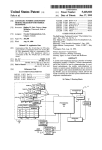
Figure 1: Analytical curve-of-growth showing the (reduced!) equivalent width (integrated from
v = −100 to v = +100) as a function of η0 , assuming α = 0.01. Black: disk-center, red: flux.
The dashed lines have slopes 0.5 and 1.0. Diamonds show the numerical results obtained with
LINFOR3D (integration from v = −50 to v = +50).
The results of a number of test calculations are listed below. The wavelength resolution was
chosen to be 1/10 of the Doppler width: δλ = 0.1 λ0 ∆vD /c. The wavelength range was set to
3.5
Grey test case
15
±50 Doppler widths; ∆vD = 6 km/s, α = 0.01. The line file used for the test calculations is
shown below.
alam
Vdop
eta0
avgt
dlam
ddlam
7
7
Test
grey sf Vdop=2.D-5, eta0=1.0D-2, avgt=1.D-2
1
7
4000.000 2.0D-5
1.0D-2
1.0D-2 4.00D0 0.80D-2
Test
grey sf Vdop=2.D-5, eta0=1.0D-1, avgt=1.D-2
1
7
4000.000 2.0D-5
1.0D-1
1.0D-2 4.00D0 0.80D-2
Test
grey sf Vdop=2.D-5, eta0=1.0D0, avgt=1.D-2
1
7
4000.000 2.0D-5
1.0D0
1.0D-2 4.00D0 0.80D-2
Test
grey sf Vdop=2.D-5, eta0=1.0D1, avgt=1.D-2
1
7
4000.000 2.0D-5
1.0D1
1.0D-2 4.00D0 0.80D-2
Test
grey sf Vdop=2.D-5, eta0=1.0D2, avgt=1.D-2
1
7
4000.000 2.0D-5
1.0D2
1.0D-2 4.00D0 0.80D-2
Test
grey sf Vdop=2.D-5, eta0=1.0D3, avgt=1.D-2
1
7
4000.000 2.0D-5
1.0D3
1.0D-2 4.00D0 0.80D-2
Test
grey sf Vdop=2.D-5, eta0=1.0D4, avgt=1.D-2
1
7
4000.000 2.0D-5
1.0D4
1.0D-2 4.00D0 0.80D-2
clam
gfscale
-4000.000
1.0
For the following tabulations we have defined
∆WI = log10 WI (linfor3D) − log10 WI (Eq.(75) ,
(77)
and
∆WF = log10 WF (linfor3D) − log10
5
WI (Eq.(75) ,
6
These results are obtained with intline=1:
η0
1.0E-02
1.0E-01
1.0E+00
1.0E+01
1.0E+02
1.0E+03
1.0E+04
∆WI
[dex]
+0.000342
+0.000331
+0.000269
+0.000072
−0.000820
−0.005441
−0.021428
ntheta=−3
+0.000336
+0.000327
+0.000271
+0.000081
−0.000807
−0.005432
−0.021421
∆WF
ntheta=3
−0.002949
−0.002958
−0.003014
−0.003203
−0.004088
−0.008714
−0.024704
These results are obtained with intline=-2:
ntheta=4
−0.001690
−0.001698
−0.001755
−0.001942
−0.002831
−0.007456
−0.023446
(78)
16
3
η0
1.0E-02
1.0E-01
1.0E+00
1.0E+01
1.0E+02
1.0E+03
1.0E+04
∆WI
[dex]
+0.000334
+0.000324
+0.000261
−0.000063
−0.000825
−0.005447
−0.021432
ntheta=−3
+0.000328
+0.000320
+0.000263
+0.000074
−0.000814
−0.005438
−0.021425
BASIC EQUATIONS OF RADIATIVE TRANSFER
∆WF
ntheta=3
−0.002957
−0.002965
−0.003022
−0.003211
−0.004097
−0.008720
−0.024708
ntheta=4
−0.001698
−0.001706
−0.001762
−0.001950
−0.002838
−0.007463
−0.023450
17
4
Program Files and Data input files
In this section all the program files making up the LINFOR3D package are listed. First an overview
on the program flow and the structures in common block linfordata is given. The format of
the data input files is described since the primary way the user controls the program execution is
via the control parameters read from linfor_setcmd.pro (see Section 5). The line parameters
are specified in the input file line.dat (see Section 6).
4.1
Main program flow
Basically, the calling sequence is as follows (incomplete listing of linfor 3D.pro):
• Read input parameters (linfor setcmd.pro)
• Initialize atomic data (linfor atom.pro
• Read line data: (linfor rdline.pro)
• Initialize ionopa abundances, opacity tables and EOS tables
• Set constants (linfor init)
• Define ff, type linfor flowfield (linfor flowfield define.pro)
• Define f1, type linfor flowfield: (linfor flowfield define.pro)
• Define fx, type linfor flowfield: (linfor flowfield define.pro)
• Define ss, type linfor spectrum: (linfor spectrum define.pro)
• Define s1, type linfor spectrum: (linfor spectrum define.pro)
• Define sx, type linfor spectrum: (linfor spectrum define.pro)
• Read model data into ff structure (linfor rduio.pro)
• Recompute model on refined z-grid (linfor regrid.pro)
• Compute ionopa quantities (pe, kappa, zeta) and monochromatic tau for 3D model
(linfor ionopa 3d.pro)
• Construct 1D reference atmosphere from ff, store in f1: (linfor refatm.pro)
• Compute ionopa quantities (pe, kappa, zeta) and monochromatic tau for 1D reference atmosphere (linfor ionopa 3d)
• Do radiative transfer calculations for 3D model (linfor dort.pro)
• Do radiative transfer calculations for averaged 3D atmosphere (linfor dort.pro)
• Store results for later evaluation (linfor eval, ss, s1, nf, kl)
• Make Plots of line profiles and bisectors (linfor plot1.pro)
• Do radiative transfer calculations for 1D reference atmosphere (linfor dort.pro)
• Store results for later evaluation (linfor evalx.pro)
• Create postcript file(s) (linfor plot2.pro)
• Generate output files linfor 3D 1.idlsave, linfor 3D 2.idlsave
• Free pointers to structures ff, f1, fx, ss, s1, and sx if free flag = 1 (see Sect. 5.1)
(linfor flowfield free.pro)
18
4.2
4
PROGRAM FILES AND DATA INPUT FILES
Structures in Common Block linfordata
Table 1 shows a list of the structrues in common block ‘linfordata’ used by the linfor 3D package.
Structure
atom
const
cmd
line
gas
eos
result
Defined in
linfor_atom.pro
linfor_init.pro
linfor_setcmd.pro
linfor_rdline.pro
linfor_init.pro
linfor_init.pro
linfor_init.pro
Description
Atomic weights & ionization potentials
Physical & model constants
Input parameters controlling program execution
Line data derived from ‘line.dat’
GAS tables initialized by ‘tabinter rdcoeff’
EOS tables initialized by ‘tabinter rdcoeff’
Basic results for computing abundance corrections
Table 1: List of all structures in common block ‘linfordata’: the table shows the name of the
structure, the routine where it is defined, and a description.
4.3
IDL Files
Table 3 shows a list of all source files necessary to run LINFOR3D. Finally, you will also need the
files which are listed in Tab. 2:
File name
blam.pro
monocubic.pro
ms_int.pro
Type
F
F
F
Description
Computes the Kirchhoff-Planck function.
Performs monotonic piecewise cubic interpolation.
Integrates a given function over optical depth.
Table 2: List of additional IDL modules which not unique to LINFOR3D.
4.3
IDL Files
19
File name
linfor_3D.pro
linfor_flowfield__define.pro
linfor_spectrum__define.pro
linfor_raysys__define.pro
linfor_atom.pro
linfor_setwts.pro
linfor_setcmd.pro
linfor_rdxatm.pro
Type
S
S
S
S
S
S
S
S
linfor_rdatlas9.pro
linfor_rdatmos.pro
linfor_rdf15.pro
S
S
S
linfor_rdsav.pro
linfor_rduio.pro
linfor_rdvog.pro
linfor_findff.pro
linfor_rdline.pro
linfor_init.pro
linfor_bisector.pro
S
S
S
S
S
S
S
linfor_convol.pro
S
linfor_dort.pro
S
linfor_eval.pro
linfor_evalx.pro
linfor_incline.pro
linfor_ionopa_3d.pro
S
S
S
S
linfor_rad3.pro
linfor_refatm.pro
linfor_regrid.pro
linfor_tauinfo.pro
linfor_ztau.pro
linfor_plot0.pro
linfor_plot1.pro
linfor_plot2.pro
(linfor_plot3.pro)
alpha_line.pro
eta0.pro
rrca.pro
vdop.pro
linfor_timing.pro
linfor_timing_print.pro
S
S
S
S
S
S
S
S
S
F
F
F
F
S
S
Description
main program
Definition of flow field structure
Definition of spectrum structure
Definition of ray system structure
Defines atomic data
Defines weights for angle quadrature
Command file, parameter input
Reads 1D reference atmosphere,
calling linfor_rdatmos or linfor_rdatlas9
Reads ATLAS9 1D atmosphere (atm.dat)
Reads ATMOS 1D atmosphere (atm.dat)
Reads a sequence of FOR15 snapshots
from 2D Kiel hydro simulations (FOR15)
Reads 3D snapshot from Copenhagen code (savfs)
Reads 3D snapshot from CO5 BOLD uio output files
Reads 3D snapshot from Voegler MHD code
Finds cached flow fields
Reads line data (line.dat)
Initializes ionopa, EOS, Opacities, several constants
Computes line bisector positions
called by linfor_plot1 and linfor_plot2
Convolves line profile with Gauss kernel
called by linfor_plot1 and linfor_plot2
Computes spectrum from flow field
(main RT module calling several lower level routines)
Evaluates mean spectrum, “abundance corrections”
Evaluates reference spectrum, “abundance corrections”
Inclines 3D flow field, called by linfor_ztau
Calculates electron pressure, ionization fractions,
and monochromatic optical depth for given flow field
Integration of RT equation
Define 1D reference atmosphere from 3D flow field
Cut out surface layers from original model, re-define grid
Prints information about optical depth scales
Prepares bundle of (inclined) rays on monochromatic tau
Plots flow field
Plots spatially resolved line profiles
Plots averaged line profiles
Plots monochromatic granulation images
Computes α-parameter for VOIGT function
Computes η0 , the opacity at line center of metal lines
Computes mean square orbital radius of electron (Uns¨
old)
Computes (thermal+turbulent) Doppler velocity [cs ]
Prepares and gathers timing statistics.
Print timing statistics
Table 3: List of all IDL modules: the table shows the file name, the type (Subroutine or Function,
and its description.
20
5
5
PARAMETER INPUT: LINFOR SETCMD.PRO
Parameter Input: linfor setcmd.pro
The input parameters (except for those defined in line.dat, see Sect. 6) are basically specified
by editing the routine linfor setcmd.pro. In this way, the user defines the structure cmd (see
Table 1). The order of entries is irrelevant. Parameters which are not required may be omitted.
A detailed explanation of the various input parameters and their possible values is given in the
following sections. An example follows in Sect. 5.9.
5.1
Program execution flags
The user can control the program execution by setting the flags run_flag, nlte_flag, cv1_flag,
cv2_flag, cv3_flag, plt_flag, maps_flag, cc3d_flag, rdbb_flag, free_flag, which are explained in more detail below.
5.1.1
run flag
function
required
type
values
:
:
:
:
program mode
always
integer
−2, −1, 0, 1, 2, 3 (usually 3)
This parameter determines the general function of LINFOR3D:
Setting run flag =-2 allows you to compute 3x3 file for the external reference model
only.
Setting run flag =-1 allows you to restore old results, and replace the results of the previous 1D external atmosphere with those of a different 1D external atmosphere.
Setting run flag = 0 (similar to run flag = -1) allows you to quickly compare the 3D
spectra with another external 1D reference atmosphere. Finally, the results are saved in files
’linfor 3D 1.idlsave’ and ’linfor 3D 2.idlsave’. Rarely used setting.
Setting run flag = 1 is used for plotting the structure of the input model on the original grid. No radiative transfer calculations are done.
Setting run flag = 2 is used for plotting the structure of the input model on the reduced (refined) grid. No radiative transfer calculations are done.
Setting run flag = 3 is the usual case. After construction of the 3D atmosphere on the
reduced (refined) grid and of the 1D mean atmosphere, the line formation calculations are
done, and the results are plotted (‘linfor plot1’: spatially and temporally resolved line profiles
and bisectors, ‘linfor plot2’: surface and time averaged line profiles and bisectors). Finally, the
results are saved in files ’linfor 3D 1.idlsave’ and ’linfor 3D 2.idlsave’.
5.1
Program execution flags
run_flag value
-1
:
0
:
1
2
3
:
:
:
5.1.2
21
control of program flow
restore results, (compute 1D ref. atmosphere & spectrum),
save results
restore results, (compute 1D ref. atmosphere & spectrum),
plot2, save results
compute 3D, 1D atmospheres
(1), plot01, stop
compute 3D, 1D atmospheres (1,2), plot02, stop
compute 3D, 1D atmospheres (1,2), line formation,
plot1, plot2, save results
cv1 flag
function
required
type
values
:
:
:
:
enforce hρ ux i = 0
always
integer
0, 1
The parameter cv1 flag controls whether or not the x-component of the velocity field is adjusted
to ensure zero mass flux in x-direction. (0: no, 1: yes). Default 0
5.1.3
cv2 flag
function
required
type
values
:
:
:
:
enforce hρ uy i = 0
always
integer
0, 1
The parameter cv2 flag controls whether or not the y-component of the velocity field is adjusted
to ensure zero mass flux in y-direction. (0: no, 1: yes). Default 0
5.1.4
cv3 flag
function
required
type
values
:
:
:
:
enforce hρ uz i = 0
always
integer
0, 1
The parameter cv3 flag controls whether or not the z-component of the velocity field is adjusted
to ensure zero mass flux in z-direction. (0: no, 1: yes). Default 0
5.1.5
plt flag
function
required
type
values
:
:
:
:
plotting of bisectors
always
integer
−1, 0, 1
The parameter plt flag controls if line bisctors should be plotted or not (0: no, 1: yes). If
plt flag is set to −1, all plotting is suppressed.
22
5.1.6
5
PARAMETER INPUT: LINFOR SETCMD.PRO
maps flag
function
required
type
values
:
:
:
:
controls output of intensity maps
always
integer
0, 1, 2
The parameter maps flag controls the output of intensity maps which are provided in the IDL
structure MAPS:
value
0
1
meaning
Continuum images only. Create map ICLAM0.
Continuum images (ICLAM0) plus images at the centre of the wavelength window
(ICLAM1), all at wavelength λ =clam;
Continuum images (ICLAM0) plus images (ICLAM2) at all wavelengths within the
wavelength window of width 2 · dlam around the central wavelength clam:
λi = clam − dlam + i · ddlam (see Sect. 6);
:
:
2
:
5.1.7
cc3d flag
function
required
type
values
:
:
:
:
output of 3D contribution function
always
integer
0, 1
The parameter cc3d flag controls whether the 3D continuum intensity contribution function
should be saved in structure contf3d or not (0: no, 1: yes).
5.1.8
nlte flag
function
required
type
values
:
:
:
:
output of 3D contribution function
always
integer
0, 1, 2, 3
The parameter nlte flag controls whether the line transfer is performed in LTE (nlte flag=0)
or in NLTE (nlte flag=1, 2, 3). The NLTE options work only for lines with available departure
coefficients, which are read from a separate data file (see below).
value
0
1
2
3
:
:
:
:
meaning
Continuum
Continuum
Continuum
Continuum
and lines in LTE.
in LTE, line source function in LTE, line opacity in NLTE
in LTE, line opacity in LTE, line source function in NLTE,
in LTE, line opacity and source function in NLTE
5.2
General paths
5.1.9
23
free flag
function
required
type
values
:
:
:
:
free pointers in structures at end of program
always
integer
0, 1
If free flag = 1, then each run of LINFOR3D allocates fresh memory for the structures ff,
f1, fx, ss, s1, and sx. In this case the corresponding pointers are removed at the end. If you
want to examine the structures after the end of execution, you must have free flag = 0. If you
want to run the program several times in a row with different input parameters, you should set
free flag = 0 in order to avoid additional memory allocation for each run.
5.2
5.2.1
General paths
abupath
function
required
type
values
:
:
:
:
directory where ’.abu’ files and ’atom.dat’ are located
always
string
e.g. ’/home/mst/ABU/’
If abupath is not specified in the command file, the path is taken from environment variable
’LINFOR3D ABU’.
5.2.2
ff path
function
required
type
values
:
:
:
:
directory to be used for reading and writing cached flow fields
always
string
e.g. ’/data/mst/ffcache/’
24
5.2.3
5
opapath
function
required
type
values
5.2.4
5.3.1
directory with opacity tables (.opta files)
always
string
e.g. ’/home/mst/RHD/opa/dat/’
:
:
:
:
directory with GAS tables (gas *.eos files)
always
string
e.g. ’/home/mst/RHD/eos/dat/’
:
:
:
:
directory with EOS tables (eos *.eos files)
always
string
e.g. ’/home/mst/RHD/eos/dat/’
eospath
function
required
type
values
5.3
:
:
:
:
gaspath
function
required
type
values
5.2.5
PARAMETER INPUT: LINFOR SETCMD.PRO
Model data
context
function
required
type
values
value
’cobold’
’copenhagen’
’kiel’
’muram’
’grey’
:
:
:
:
source of input model
always
string
e.g. ’cobold’
meaning
3D CO5 BOLD
N&S 3D code
Kiel 2D HDW-Code
MURAM 3D MHD Code
construct grey 3D (nx = ny = 10)
hydrostatic atmosphere for test purposes
:
:
:
:
:
:
The τRoss grid of the grey atmosphere is defined by the parameters cmd.lutau1, cmd.lutau2,
cmd.dlutau. The atmospheric parameters must be specified as cmd.Teff and cmd.grav. The
opacity table must be specified as cmd.opafile, and the equation of state as cmd.eosfile and
cmd.gasfile.
5.3.2
rhdpath
function
required
type
values
:
:
:
:
directory with 2D/3D model atmospheres (.end, .full files)
always
string
e.g. ’/data/mst/model/’
5.3
Model data
5.3.3
25
modelid
function
required
type
values
:
:
:
:
name of 2D/3D model file
always
string
e.g. ’gt57g44n66 3Dgz.end’
Note: A list of files can be specified by using wildcards, e.g. ’chro3D04*.full’.
5.3.4
parfs
function
required
type
values
5.3.5
:
:
:
:
full path to parameter file (rhd.par)
CO5 BOLD only
string
e.g. ’/data/mst/model/par/gt57g44n66.par’
:
:
:
:
full path to xbc files (*.xbc)
CO5 BOLD only
string
e.g. ’/data/mst/NLTE3D data/model/’
xbcpath
function
required
type
values
Note: xbc-files are necessary for NLTE line formation calculations. Presently limited to Li for
selected CO5 BOLD models.
5.3.6
abuid
function
required
type
values
:
:
:
:
Abundance mixture to be used in ionopa-routines
always
string
’kiel’, ’cifist2006’, ’special’
abuid identifies the solar abundance mix which is then modified according to dmetal and dalpha
(see below). The corresponding tables, kiel.abu, cifist2006.abu, or special.abu must be
located in diectory abupath.
5.3.7
dmetal
function
required
type
values
:
:
:
:
metallicity [M/H] (log10 ) to be used in ionopa-routines
always
float
e.g. 0.0, −0.5, −2.0
The logarithmic abundance of all elements beyond Li (N > 3) is changed by dmetal.
26
5
5.3.8
PARAMETER INPUT: LINFOR SETCMD.PRO
dalpha
function
required
type
values
:
:
:
:
alpha enhancement to be used in ionopa-routines
always
float
e.g. 0.0, +0.4
The logarithmic enhancement factor to be applied to all α-elements (O Ne Mg Si S Ar Ca Ti).
5.3.9
nx skip
function
required
type
values
:
:
:
:
sampling of model in x-direction
if context=’cobold’,’kiel’,’muram’
integer
1, 4, 10; −1
If both nx skip and ny skip (see Sect. 5.3) are negative, the original data are re-binned from
(nx,ny) to (nx/abs(nx skip),ny/abs(ny skip)). In the usual case that both nx skip and
ny skip are positive, the original data are re-sampled, skipping by nx skip in x, and by ny skip
in y-direction (nx/nx skip, and ny/ny skip should preferably be an integer). If nx skip and
ny skip have different signs, an error message is printed and the program is stopped. The value
1 has no effect.
5.3.10
ny skip
function
required
type
values
:
:
:
:
sampling of model in x-direction
if context=’cobold’,’kiel’,’muram’
integer
1, 4, 10; −1
For details see description of nx skip (Sect. 5.3).
5.4
More model information (all read from parameter file for CO5 BOLD data)
The parameters in this section are ignored in the case of CO5 BOLD data and instead read from
the specified CO5 BOLD parameter file.
5.4.1
opafile
function
required
type
values
:
:
:
:
name of opacity file (binned opacity tables)
not needed if context=’cobold’
string
e.g. ’g2v.opta’
5.4
More model information (all read from parameter file for CO5 BOLD data)
5.4.2
gasfile
function
required
type
values
5.4.3
opacity scale height [cm] at top of 3D model
not needed if context=’cobold’
float
e.g. 60.0E5
:
:
:
:
mean molecular weight of neutral gas
not needed if context=’cobold’
float
e.g. 1.301855
:
:
:
:
effective temperature of 3D model
not needed if context=’cobold’
float
e.g. 5770.0
:
:
:
:
surface gravity [cm/s2 ] of 3D model
not needed if context=’cobold’
float
e.g. 27500.0
:
:
:
:
surface temperature (τ = 0) of 3D model is tsurffac·Teff
not needed if context=’cobold’
float
e.g. 0.727903
grav
function
required
type
values
5.4.8
:
:
:
:
Teff
function
required
type
values
5.4.7
name of EOS file (ρ, e → P, T, . . .)
not needed if context=’cobold’
string
e.g. ’eos mm00 l.eos’
qmol
function
required
type
values
5.4.6
:
:
:
:
htau0
function
required
type
values
5.4.5
name of GAS file (P, T → ρ, e, . . .)
not needed if context=’cobold’
string
e.g. ’gas mm00 l.eos’
eosfile
function
required
type
values
5.4.4
:
:
:
:
tsurffac
function
required
type
values
27
28
5.5
5
PARAMETER INPUT: LINFOR SETCMD.PRO
Model data - reading of ’full’ files (CO5 BOLD only)
The parameters in this section are only needed for reading snapshot from CO5 BOLD data files.
5.5.1
isnap full 1
function
required
type
values
5.5.2
first snapshot to be read from full file(s)
only needed if context=’cobold’
integer
1
isnap full 2
function
required
type
values
5.5.3
:
:
:
:
:
:
:
:
last snapshot to be read from full file(s)
only needed if context=’cobold’
integer
1
:
:
:
:
step for reading snapshots from full file(s)
only needed if context=’cobold’
integer
1
istep full
function
required
type
values
5.6
h3Di mean model
5.6
h3Di mean model
5.6.1
mavg
function
required
type
values
value
1
4
5.7
29
:
:
:
:
:
:
mode of averaging 3D T-structure on τRoss
always
integer
1, 4
meaning
Th3Di (τRoss ) = hT3D (τRoss )i
4 (τ
1/4
Th3Di (τRoss ) = hT3D
Ross )i
External 1D reference model
5.7.1
atmpath
function
required
type
values
5.7.2
:
:
:
:
directory with 1D model atmospheres
always
string
e.g. ’/home/mst/atm/’
:
:
:
:
name of 1D reference model
always
string
e.g. ’NONE’, ’falc.atm’
atmfile
function
required
type
values
Note: No external 1D reference atmosphere will be used if atmfile=’NONE’. In this case the
parameter atmpath has no meaning.
5.8
Line data and radiative transfer
5.8.1
linfs
function
required
type
values
:
:
:
:
name of line data file
always
string
e.g. ’Li67.line’
Note: If linfs is not specified, the default value ’line.dat’ is assumed.
30
5.8.2
5
lutau1
function
required
type
values
5.8.3
:
:
:
:
z-spacing of sub-model corresponds roughly to ∆ log τRoss =dlutau
always
float
e.g. 8.0D − 2
:
:
:
:
smallest log τcont used for RT integration
always
float
e.g. −7.0D0, ≥ lutau1
:
:
:
:
largest log τcont used for RT integration
always
float
e.g. 2.0D0, ≤ lutau2
:
:
:
:
resolution in log τcont used for RT integration
always
float
e.g. 8.0D − 2
:
:
:
:
number of θ-angles for which spectrum is computed
always
integer
0, 1, 2, 3, (−3), 4, 6, 8
dlctau
function
required
type
values
5.8.8
largest log τRoss covered by sub-model (refined z-grid
always
float
e.g. 2.0D0
lctau2
function
required
type
values
5.8.7
:
:
:
:
lctau1
function
required
type
values
5.8.6
smallest log τRoss covered by sub-model (refined z-grid)
always
float
e.g. −7.0D0
dlutau
function
required
type
values
5.8.5
:
:
:
:
lutau2
function
required
type
values
5.8.4
PARAMETER INPUT: LINFOR SETCMD.PRO
ntheta
function
required
type
values
0: Intensity spectrum, > 0: Intensity and flux spectrum;
5.8
Line data and radiative transfer
5.8.9
31
nphi
function
required
type
values
5.8.10
:
:
:
:
number of φ-angles for integration of flux spectrum
always
integer
no restriction, typically 4
:
:
:
:
view angle µ = cos θ
always
float
0.0 .. 1.0
mu0
function
required
type
values
If the parameter ntheta=0, then the spectrum and intensity maps are computed for inclination
angle mu0 (= cos θ0 ).
mu0= 1.0 corresponds to vertical rays, i.e. disk center view.
mu0= 0.0 corresponds to the very limb, but a value of mu0=0.0 will clearly not work.
5.8.11
kphi
function
required
type
values
:
:
:
:
view angle
always
integer
0, 1, 2, 3
The parameter kphi determines the direction from which the model is viewed:
value
0
:
1
:
2
:
3
:
meaning
rays emerge parallel to the x-axis, i.e. the model is viewed somewhere
on the ’equator’ between the left limb and disk center.
rays emerge parallel to the y-axis, i.e. the model is viewed somewhere
on the ’meridian’ between the lower limb and disk center.
rays emerge anti-parallel to the x-axis, i.e. the model is viewed somewhere
on the ’equator’ between the right limb and disk center.
rays emerge anti-parallel to the y-axis, i.e. the model is viewed somewhere
on the ’meridian’ between the upper limb and disk center.
Other (integer) values of kphi are allowed, but give no new results; increasing kphi by
one increases phi by π/2.
5.8.12
Hbrd
function
required
type
values
:
:
:
:
controls broadening of hydrogen lines
always
integer
0, 1, 2, 3
32
value
0
1
2
3
5
:
:
:
:
PARAMETER INPUT: LINFOR SETCMD.PRO
meaning
Cayrel & Traving (1960), default
Resonance broadening: AG , Stark boradening: G
Resonance broadening: BPO, Stark boradening: G
Resonance broadening: A08 , Stark boradening: G
AG : Ali & Griem (1966, Phys. Rev. 144, 366),
BPO: Barklem, Piskunov and O’Mara (2000, A&A 363, 1091),
A08 : Allard et al. (2008, A&A 480, 581),
G : Griem (1960, ApJ 132, 883), with corrections to approximate the Vidal, Cooper & Smith
(1973, ApJS 25, 37) profiles.
Note: option Hbrd=2 has an effect only on Hα, Hβ, and Hγ, and Hbrd=3 affects only Hα;
all other hydrogen lines are treated according to option Hbrd=1, unless Hbrd=0.
5.8.13
5.8.14
5.8.15
5.8.16
ximicx
function
:
required
type
values
:
:
:
isotropic Gaussian microturbulence velocity [km/s] for external
1D reference model (added quadratically to thermal velocity)
always
float
e.g. 1.0
ximic1
function
:
required
type
values
:
:
:
isotropic Gaussian microturbulence velocity [km/s] for h3Di
mean models (added quadratically to thermal velocity)
always
float
e.g. 1.0
ximic3
function
:
required
type
values
:
:
:
isotropic Gaussian microturbulence velocity [km/s] for 2D/3D models
(added quadratically to thermal flow velocity)
always
float
e.g. 1.0
ximacx
function
:
required
type
values
:
:
:
Isotropic Gaussian macroturbulence velocity [km/s] for external
1D reference model (additional line broadening after line formation)
always
float
e.g. 1.6
5.8
Line data and radiative transfer
5.8.17
5.8.18
5.8.19
5.8.20
5.8.21
5.8.22
33
ximac1
function
:
required
type
values
:
:
:
Isoptropic Gaussian macroturbulence velocity [km/s] for h3Di
mean models (additional line broadening after line formation)
always
float
e.g. 1.6
ximac3
function
:
required
type
values
:
:
:
Isotropic Gaussian macroturbulence velocity [km/s] for 2D/3D models
(additional line broadening after line formation)
always
float
e.g. 1.6
vfacx
function
:
required
type
values
:
:
:
the x-component of the hydrodynamical velocity field of the
2D/3D models is multiplied by this factor
always
float
e.g. 0.0, 1.0
vfacy
function
:
required
type
values
:
:
:
the y-component of the hydrodynamical velocity field of the
2D/3D models is multiplied by this factor
always
float
e.g. 0.0, 1.0
vfacz
function
:
required
type
values
:
:
:
the z-component of the hydrodynamical velocity field of the
2D/3D models is multiplied by this factor
always
float
e.g. 0.0, 1.0
:
:
:
:
controls microturbulence in 1D curve-of-growth
always
integer
0, 1
micro
function
required
type
values
Determines whether or not different microturbulence values should be used when computing the
1D curve-of growth. 0: only one value, given by ximicx and ximic1, respectively; 1: sequence
34
5
PARAMETER INPUT: LINFOR SETCMD.PRO
of microturbulence values defined by parameters xi a, xi b, xi d (see below).
5.8.23
xi a
function
required
type
values
5.8.24
determines start value for microturbulence sequence
always
float
e.g. 0.0, default: 0.5
:
:
:
:
determines end value for microturbulence sequence
always
float
e.g. 2.0, default: 1.5
:
:
:
:
determines intervals of microturbulence sequence
always
float
e.g. 0.1, default: 0.125
xi b
function
required
type
values
5.8.25
:
:
:
:
xi d
function
required
type
values
The microturbulence sequence is computed as xi(i) = xi0 * (xi a + i * xi d), i=0 .. im, where
xi0 is ximicx and ximic1, respectively, and im= (xi b - xi a)/ xi d.
5.8.26
dclam
function
required
type
values
:
:
:
:
determines the variation of the continuum
always
float
e.g. 20.0, default: 0
if dclam=0, the continuum is treated as constant (default). Otherwise, the continuum is
computed at 3 wavelength points, clam-dclam, clam, clam+dclam, where clam is the central
wavelength (in ˚
A) of the computed spectral range (see Sect. 6), and dclam is half the width of
the specified spectral range (in ˚
A). The continuum is computed by parabolic interpolation inside
the spectral window. If the spectral range of the specified synthetic spectrum (which is defined
by the parameters of the line file (see Sect. 6) exceeds a few ˚
A, dclam should be set to match
half the total spectral range.
5.8.27
intmode
function
required
type
values
:
:
:
:
mode of integration in routines ms int tau and ms int exp
always
integer
0, 1
Determines the mode of integration in routines ms int tau and ms int exp, which can be linear
5.8
Line data and radiative transfer
35
(0) or monotonic and cubic (1, standard).
5.8.28
intline
function
required
type
values
:
:
:
:
mode of integrating the line transfer equation
always
integer
1, 2, −1, −2
Determines the method of integrating the line transfer equation (see Section 3 for details).
Default value is intline=1.
value
1
2
-1
-2
5.8.29
:
:
:
:
meaning
Line depression on fixed log τ scale (Eq. 41)
Line depression on monochromatic τ scale (Eq. 36)
Line intensity on fixed log τ scale (Eq. 25)
Line intensity on monochromatic τ scale (Eq. 26)
nchunk
function
required
type
values
:
:
:
:
rad.transfer is done in n chunk ”slices”
always
integer
e.g. 2
Default is nchunk = 1, i.e. the whole model is processed as one block. For large models, it may
be necessary to split the computation into several ‘chunks’ to save memory.
36
5.9
5
PARAMETER INPUT: LINFOR SETCMD.PRO
Example
pro linfor_setcmd
common linfordata
cmd = {$
;-----------------------------------------------------------------------------; Program execution flags:
nlte_flag: 0, $
; 0 / 1 / 2 / 3: LTE or NLTE for lines with xb
run_flag: 3, $
; execution mode: -2, -1, 0, 1, 2, 3
cv1_flag: 1, $
; 0 / 1: enforce <rho*v1>(z)=0 off / on
cv2_flag: 1, $
; 0 / 1: enforce <rho*v2>(z)=0 off / on
cv3_flag: 0, $
; 0 / 1: enforce <rho*v3>(z)=0 off / on
plt_flag: 1, $
; -1 / 0 / 1: plotting off / bisectors off / on
maps_flag: 1, $
; create maps ICLAM0 .. ICLAMm, m=map_flag
cc3d_flag: 0, $
; 0 / 1: output of CC3(nx,ny,nx) off / on
rdbb_flag: 0, $
; 0 / 1: Read magnetic field, write SIR output
free_flag: 0, $
; free pointers in structures at end of program
;
;-----------------------------------------------------------------------------; General paths:
abupath: ’/home/mst/idl/spesyn/Linfor_3D/ABU/’, $
; Path to abu files and atom.dat
; if not set, abupath is read from environment variable LINFOR3D_ABU
ff_path: ’/work2/mst/ffcache/’, $
; directory with cached flow fields
;
’NONE’: do not use cached flow fields
opapath: ’/home/mst/opta/’, $
; directory with opacity tables
gaspath: ’/work2/mst/eos/dat/’, $
; directory with GAS tables
eospath: ’/work2/mst/eos/dat/’, $
; directory with EOS tables
;
;-----------------------------------------------------------------------------; Model data:
context: ’cobold’, $
rhdpath: ’/work1/mst/dgt57g44n73/end/’, $
; directory with model data
modelid: ’gt57g44n73_3D[c-d]z.end’, $
; data file name
parfs:
’/work1/mst/dgt57g44n73/par/gt57g44n73_3D_d.par’, $ ; parameter file
xbcpath: ’/work2/mst/NLTE3D_data/’, $
; directory of departure coefficients
abuid: ’cifist2006’, $
; abundance mixtures ’kiel’, or ’cifist2006’
dmetal: 0.0, $
; log10 scaling for metal abundances (Z>3)
dalpha: 0.0, $
; log10 scaling for alpha elements
;
(O, Ne, Mg, Si, S, Ar, Ca, Ti)
nx_skip: 5, ny_skip: 5, $
; sampling in x, y (kiel, cobold only)
;
; more information (all read from parameter file for CO5BOLD)
opafile: ’undefined’, $
gasfile: ’undefined’, $
eosfile: ’undefined’, $
htau0: 00.0E5, $
qmol:
00.0E5, $
; mean molecular weight
teff: 5770.0, grav: 27500.0, $
; copenhagen only
tsurffac: 0.727903, $
; Surface temperature = tsurffac*Teff
;----------------------------------------------------------------------------; Reading of ’full’ files (CO5BOLD only):
isnap_full_1: 1, $
; first snapshot to be read from full file(s)
isnap_full_2: 9, $;
;
last snapshot to be read from full file(s)
istep_full:
2 $
; step for reading snapshots from full file(s)
;-----------------------------------------------------------------------------; <3D> mean model:
mavg: 4, $
; 1: T-average, 4: T^4-average for defining <3D> atmosphere
5.9
Example
;-----------------------------------------------------------------------------; External 1D reference model:
atmpath: ’/home/mst/idl/spesyn/1Dmodels/HM/’, $ ; directory of reference model
atmfile: ’atm50_shm10c.atm’, $
; name of reference model
;
’NONE’: no reference model
;-----------------------------------------------------------------------------; Line data / radiative transfer:
linfs:
’line.dat’, $
; File with line data
lutau1: -7.0D0, lutau2: 2.0D0, dlutau: 8.0D-2, $ ; tau scale defining vertical
;
model extent and resolution
lctau1: -5.0D0, lctau2: 2.0D0, dlctau: 8.0D-2, $ ; universal tau scale for
;
integration of RT equation
ntheta: 0, nphi: 4, $
; number of theta and phi angles
mu0: 0.40, kphi: 0, $
; view angle if ntheta=0 (cos theta,kphi*pi/2)
n_chunk: 1, $
; RT is done in n_chunk "slices"
;----------------------------------------------------------------------------Hbrd:
’0’, $
; option for H line broadening
; 0 - (default) Cayrel & Traving
; 1 - BPO (self reson) + Griem (stark)
; 2 - Ali-Griem (self reson) + Griem (stark)
ximicx: 1.00, $
; microturbulence [km/s], 1D-REF atmosphere
ximic1: 1.00, $
; microturbulence [km/s], 1D-AVG atmosphere
ximic3: 0.00, $
; microturbulence [km/s], 3D-RHD atmosphere
ximacx: 1.60, $
; macroturbulence [km/s], 1D-REF atmosphere
ximac1: 1.60, $
; macroturbulence [km/s], 1D-AVG atmosphere
ximac3: 0.00, $
; macroturbulence [km/s], 3D-RHD atmosphere
vfacx: 1.00, $
; fudge factor for 3D x-velocity
vfacy: 1.00, $
; fudge factor for 3D y-velocity
vfacz: 1.00, $
; fudge factor for 3D z-velocity
micro:
0, $
; compute microturbulence sequence (0/1)
xi_a: 0.0, xi_b: 2.0, xi_d: 0.1, $ ; start, stop, delta of micro sequence
dclam: 0.0, $ ; variation of continuum from clam-dclam .. clam+dclam [A]
intmode: 1, $
; integration mode (linfor_msint)
intline: 1, $
; line integration: depth (1,2) / I (-1,-2)
;
}
;
end
37
38
6
6
LINE DATA FILE: LINE.DAT
Line Data File: line.dat
There are several different formats (for historical reasons) to specify line data which are described
in Sect. 6.2.
Note that all formats were extended in version 1.5.0 and now do have to contain the two lines
clam
2000.0
gfscale
1.0
at the end. These parameters are explained in Sect. 6.1. Some helpful remarks concerning the
conversion of line broadening parameters are given in Sect. 6.3.
6.1
6.1.1
Parameters in Line Data File
clam
function
required
type
values
:
:
:
:
continuum wavelength in ˚
A, also center of wavelength window
always
float
e.g., 2000.0
clam defines the wavelength where the continuum opacities are computed, and also defines the center of the window for which spectrum synthesis is done. The window extends from λ =clam-dlam
to λ =clam+dlam, depending on the value of dlam specified for the particular line.
From Version 3.1.2, a negative clam indicates that the continuum source function is to be set
to the wavelenth-integrated Planck-Function, S = σ T 4 /π, and the continuum opacity is set to
the Rosseland mean opacity, κcont = κRoss ..
6.1.2
gfscale
function
required
type
values
:
:
:
:
global scaling factor for oscillator strengths
always
float
e.g., 1.0
Note: The value 1 has no effect.
6.2
6.2.1
Line Data Formats
Continuum only
It is possible to do pure continuum calculations. In this case, the ‘line.dat’ file looks like this.
Example:
Some text header
1
1
Continuum, 2000 A
1
-1
clam
gfscale
2000.0
1.0
Description of entries:
Row 1: Header (identifies the meaning of the columns for data in row 5)
Row 2: Two integers, kline and ktotal; both of them must be 1
6.2
Line Data Formats
Row
Row
Row
Row
3:
4:
5:
6:
39
String, identifier of the continuum calculation
Two integers, nbl = 1, incode = −1
Description for data in row 6
clam and gfscale (see Sect.6.1)
All the line parameters remain undefined.
6.2.2
Single line calculations, line data format ‘0’
For a single unblended line, the simplest form of the ‘line.dat’ file looks like this.
Example:
Mult
namj
ei
1
1
Fe I, 5500 A, 0.00 eV
1
0
0000
2600
0.000
clam
gfscale
2000.0
1.0
alam
gflg
dlgC6
drrca1
dlam
ddlam
5500.0
-6.000
1.0
10.0
5.5D-1 5.5D-3
Description of entries:
Row 1: Header (identifies the meaning of the columns for data in row 5)
Row 2: Two integers, kline and ktotal
kline: number of line calculations requested in this file
ktotal: is the total number of spectral lines including blends
in this case kline = 1, ktotal = 1
Row 3: String, identifier of the (first) line calculation
Row 4: Integer nbl, integer array incode(nbl)
nb: number of blend components for this line calculation (= 1)
incode: integer array identifying the input format for each of the blend components (= 0)
Row 5: Line data in format ‘0’ (7 + 2 columns):
C1: Multiplet number (for information only)
C2: Identifier of atom or ion (e.g. 2601 mean FeII)
C3: Excitation potential of lower level in [eV]
C4: Central wavelength of blend component
C5: log gf value of blend component
C6: ∆ log C6 : Enhancement factor for van der Waals line broadening
C7: ∆r2 /a20 : Difference of mean square electron orbital radii
C8: ∆λ [˚
A]: Line profile is computed from λ0 − ∆λ to λ0 + ∆λ
˚
C9: δλ [A]: Spacing of wavelength points for spectrum synthesis
(C10: W0 [m˚
A]: total equivalent width of this blend, see below)
Row 6: Description for data in row 6
Row 7: clam and gfscale (see Sect.6.1)
In this case, the Stark broadening (due to collisions with electrons) is neglected (C4 = 0).
Radiative damping (γrad ) is treated in the classical approximation.
In the case of a single blended line the ‘line.dat’ file looks as follows:
Example:
40
6
Mult
namj
ei
alam
gflg
1
2
Fe I, 0.00 eV + Fe II, 3.00 eV, 2000 A
2
0 0
9999
2600
0.000
2000.0
-6.441
9999
2601
3.000
2000.0
-4.550
clam
gfscale
2000.0
1.0
LINE DATA FILE: LINE.DAT
dlgC6
drrca1
dlam
ddlam
1.0
1.0
10.0
10.0
1.5D-1 1.5D-3
Note that it is not necessary that the blend components belong to the same ion. Here kline = 1,
ktotal = 2, nbl = 2, incode = [0, 0]. Note that only the last of the rows describing the blend need
entries C8 and C9.
With a slight modification, it is possible to enter an equivalent width (W0 in [m˚
A]) in
column C10. For this purpose, nbl must be negative, with |nbl| being the number of blend
components. The gf value producing this equivalent width W0 is returned in result.gflg01
(average 3D atmosphere) and result.gflg0x (1D reference atmosphere).
Example unblended line:
Mult
namj chik
alam
1 1
N I Fictitious Line 1: /
-1 0
9999
700
0.000
5500.0
clam
gfscale
2000.0
1.0
gflg
dlgC6
drrca1
0.000
5500.0
-7.6914
-7.6914
1.00
10.00
dlam
ddlam
1.00
3.00E-01
10.00
W0
75.00 /
3.00E-03
75.00
dlam
ddlam
W0
1.50D-1
1.50D-03
100.00
Example blended line:
Mult
namj chik
alam
gflg
dlgC6
1 2
Fe I, 0.00 eV + Fe II, 3.00 eV, 2000 A
-2 0 0
9999
2600 0.000
2000.0
-6.441
1.0
9999
2601 3.000
2000.0
-4.550
1.0
clam
gfscale
2000.0
1.0
6.2.3
drrca1
10.0
10.0
Single line calculations, line data format ‘1’
For a single unblended line, the this form of the ‘line.dat’ file looks like this.
Example:
Mult
namj
ei
alam
gflg
dlgC6 lu
1
1
O I ApJ Line 2: 92 6300.30 0.000 -9.773
1
1
92
800
0.000 6300.30 -9.773
1.0
1
clam
gfscale
2000.0
1.0
diu
lo
dio
dlam
ddlam
0.0
2
0.0
4.D-1
4.D-3
Description of entries:
Row 1: Header (identifies the meaning of the columns for data in row 5)
Row 2: Two integers, kline and ktotal
6.2
Line Data Formats
Row 3:
Row 4:
Row 5:
Row 6:
Row 7:
41
kline: number of line calculations requested in this file
ktotal: is the total number of spectral lines including blends
in this case kline = 1, ktotal = 1
String, identifier of the (first) line calculation
Integer nbl, integer array incode(nbl)
nb: number of blend components for this line calculation (= 1)
incode: integer array identifying the input format for each of the blend components (= 1)
Line data in format ‘1’ (10 + 2 columns):
C1: Multiplet number (for information only)
C2: Identifier of atom or ion (e.g. 2601 mean FeII)
C3: Excitation potential of lower level in [eV]
C4: Central wavelength of blend component
C5: log gf value of blend component
C6: ∆ log C6 : Enhancement factor for van der Waals line broadening
C7: LU : Orbital quantum number of valence electron of lower level
C8: DIU : excitation energy [eV ] of parent term for lower level
C9: LO: Orbital quantum number of valence electron of upper level
C10: DIO: excitation energy [eV ] of parent term for upper level
C11: ∆λ [˚
A]: Line profile is computed from λ0 − ∆λ to λ0 + ∆λ
A]: Spacing of wavelength points for spectrum synthesis
C12: δλ [˚
(C13: W0 [m˚
A]: total equivalent width of this blend, see below)
Description for data in row 6
clam and gfscale (see Sect.6.1)
In this case, ∆r2 /a20 is computed from LU , DIU , LO, DIO (Function rrca). As before, the
Stark broadening (due to collisions with electrons) is neglected (C4 = 0). Radiative damping
(γrad ) is treated in the classical approximation.
In the case of a single blended line the ‘line.dat’ file looks as follows:
Example:
Mult
namj
ei
alam
gflg
dlgC6
1
3
O I ApJ Line 1: 67 6158.17 10.741 -1.140
3
1 1 1
67
800
10.741 6158.15 -1.985
1.0
67
800
10.741 6158.17 -1.140
1.0
67
800
10.741 6158.19 -0.553
1.0
clam
gfscale
2000.0
1.0
lu
diu
lo
dio
dlam
ddlam
1
1
1
0.0
0.0
0.0
2
2
2
0.0
0.0
0.0
4.D-1
4.D-3
Here kline = 1, ktotal = 3, nbl = 3, incode = [1, 1, 1]. Note that only the last of the rows
describing the blend need entries C11 and C12.
As in the case of format ’0’, it is possible to enter an equivalent width (W0 in [m˚
A]) in
column C13. For this purpose, nbl must be negative, with |nbl| being the number of blend
components. The gf value producing this equivalent width W0 is returned in result.gflg01
(average 3D atmosphere) and result.gflg0x (1D reference atmosphere).
Example unblended line:
Mult
1 1
namj
ei
alam
gflg
dlgC6 lu
diu
lo
dio
dlam
ddlam
W0
42
6
O I ApJ Line 2: 92
-1 1
92
800
0.000
clam
gfscale
2000.0
1.0
6300.30
0.000 -9.773
6300.30
-9.773 1.0
1
LINE DATA FILE: LINE.DAT
0.0
2
0.0
4.D-1 4.D-3
7.00
diu
lo
dio
dlam
W0
0.0
0.0
0.0
2
2
2
0.0
0.0
0.0
4.D-1 4.D-3 10.00
Example blended line:
Mult
namj
ei
1 3
O I ApJ Line 1: 67
-3 1 1 1
67
800 10.741
67
800 10.741
67
800 10.741
clam
gfscale
2000.0
1.0
6.2.4
alam
gflg
dlgC6 lu
ddlam
6158.17 10.741 -1.140
6158.15
6158.17
6158.19
-1.985 1.0
-1.140 1.0
-0.553 1.0
1
1
1
Single line calculations, complete line data format ‘2’
For a single unblended line, the this form of the ‘line.dat’ file looks like this.
Example:
Mult
namj
ei
alam
gflg
dlgC6 drrca1 dlgC4 C4lg
dlggr
1
1
Si I AA Line 5: 16
5948.540 5.0823 -1.130 390.03
11.80 -1 86
1
2
16 1400
5.0823 5948.540 -1.130 1.0
390.03 0.0
11.80 0.0
clam
gfscale
2000.0
1.0
Crad
dlam
ddlam
-1.0
5.D-1
5.D-3
Description of entries:
Row 1: Header (identifies the meaning of the columns for data in row 5)
Row 2: Two integers, kline and ktotal
kline: number of line calculations requested in this file
ktotal: is the total number of spectral lines including blends
in this case kline = 1, ktotal = 1
Row 3: String, identifier of the (first) line calculation
Row 4: Integer nbl, integer array incode(nbl)
nb: number of blend components for this line calculation (= 1)
incode: integer array identifying the input format for each of the blend components (= 2)
Row 5: Line data in format ‘2’ (11 + 2 columns):
C1: Multiplet number (for information only)
C2: Identifier of atom or ion (e.g. 2601 mean FeII)
C3: Excitation potential of lower level in [eV]
C4: Central wavelength of blend component
C5: log gf value of blend component
C6: ∆ log C6 : Enhancement factor for van der Waals line broadening
C7: ∆r2 /a20 : Difference of mean square electron orbital radii
C8: ∆ log C4 : Enhancement factor for Stark line broadening
C9: − log C4 : Stark broadening constant.
if − log C4 < 0 (typically − log C4 = −1.0), then C4 = 0
if − log C4 = 0, then use Griem (Phys. Rev. 165, 258, 1968)
6.2
Line Data Formats
43
and Cowley (Obs. 91, 139, 1971) approximation
C10: ∆ log γrad : Enhancement factor for natural line broadening
C11: Crad : Natural line broadening (10−8 γrad )
if Crad < 0, use classical formula (γrad = 2.22 · 1015 /λ2 ) [1/s], where λ is in ˚
A.
C12: ∆λ [˚
A]: Line profile is computed from λ0 − ∆λ to λ0 + ∆λ
C13: δλ [˚
A]: Spacing of wavelength points for spectrum synthesis
(C14: W0 [m˚
A]: total equivalent width of this blend, see below)
Row 6: Description for data in row 6
Row 7: clam and gfscale (see Sect.6.1)
In the case of a single blended line the ‘line.dat’ file looks as follows:
Example:
Mult
namj
ei
alam
gflg
dlgC6 drrca1 dlgC4 C4lg
dlggr Crad
1
2
Si I / Si II blend: 16
5948.540 5.0823 -1.130 390.03
11.80 -1 86
2
2 2
16 1400
5.0823 5948.540 -1.130 1.0
390.03 0.0
11.80 0.0
-1.0
16 1401
0.0823 5948.530 -3.130 1.0
90.00 0.0
13.80 0.0
-1.0
clam
gfscale
2000.0
1.0
dlam
ddlam
5.D-1
5.D-3
Here kline = 1, ktotal = 2, nbl = 2, incode = [2, 2, 2]. Note that only the last of the rows
describing the blend need entries C12 and C13.
As in the cases of format ’0’ and ’1’, it is possible to enter an equivalent width (W0 in [m˚
A])
in column C14. For this purpose, nbl must be negative, with |nbl| being the number of blend
components. The gf value producing this equivalent width W0 is returned in result.gflg01
(average 3D atmosphere) and result.gflg0x (1D reference atmosphere). No examples are given
since the necessary modification the the data format should be obvious.
6.2.5
Single line calculations, complete line data format ‘3’
This data format has a maximum of 17 columns. It differs from format ‘2’ only in the way the
van der Waals broadening parameters are specified. Columns C7 with ∆r2 /a20 is replaced by the
four columns:
C7: LU : Orbital quantum number of valence electron of lower level
C8: DIU : excitation energy [eV ] of parent term for lower level
C9: LO: Orbital quantum number of valence electron of upper level
C10: DIO: excitation energy [eV ] of parent term for upper level
as in format ‘1’. The remaining columns are as in format ’2’, but shifted by +3:
C11: ∆ log C4 : Enhancement factor for Stark line broadening
C12: − log C4 : Stark broadening constant.
if − log C4 < 0 (typically − log C4 = −1.0), then C4 = 0
if log C4 = 0, then use Griem (Phys. Rev. 165, 258, 1968)
and Cowley (Obs. 91, 139, 1971) approximation
C13: ∆ log γrad : Enhancement factor for natural line broadening
C14: Crad : Natural line broadening (10−8 γrad )
if Crad < 0, use classical formula (γrad = 2.22 · 1015 /λ2 ) [1/s], where λ is in ˚
A.
C15: ∆λ [˚
A]: Line profile is computed from λ0 − ∆λ to λ0 + ∆λ
44
6
LINE DATA FILE: LINE.DAT
C16: δλ [˚
A]: Spacing of wavelength points for spectrum synthesis
(C17: W0 [m˚
A]: total equivalent width of this blend, see below)
This format has not yet been used or tested, and no example files are available.
As in the cases of format ’0’, ’1’, and ’2’ it should also be possible to enter an equivalent
width (W0 in [m˚
A]), now in column C17. For this purpose, nbl must be negative, with |nbl| being
the number of blend components. The gf value producing this equivalent width W0 is returned
in result.gflg01 (average 3D atmosphere) and result.gflg0x (1D reference atmosphere).
6.2.6
Single line calculations, complete line data format ‘7’
This data format was designed for simple test calculations where the line profile is fixed, i.e. the
line parameters are depth-independent (see also Sect. 3.5). This format has a maximum of 7
columns:
Description of entries:
Row 1: Header (identifies the meaning of the columns for data in row 5)
Row 2: Two integers, kline and ktotal
kline: number of line calculations requested in this file
ktotal: is the total number of spectral lines including blends
in this case kline = 1, ktotal = 1
Row 3: String, identifier of the line calculation
Row 4: Integer nbl, integer array incode(nbl)
nb: number of blend components for this line calculation (= 1)
incode: integer array identifying the input format for each of the blend components (= 7)
Row 5: C1: Central wavelength of blend component [˚
A]
C2: Doppler broadening in units of c, vD /c
C3: η0 = κline /κcont at line center
C4: α-parameter for Voigt profile, α = γ/2/∆ωD
(ratio of half half width of dispersion profile and Doppler widths of Gaussian).
C5: ∆λ [˚
A]: Line profile is computed from λ0 − ∆λ to λ0 + ∆λ
C6: δλ [˚
A]: Spacing of wavelength points for spectrum synthesis
(C7: W0 [m˚
A]: total equivalent width of this blend, see above)
Row 6: Description for data in row 6
Row 7: clam and gfscale (see Sect.6.1)
Example:
alam
Vdop
eta0
avgt
dlam
ddlam
1
1
Test
grey sf Vdop=2.D-5, eta0=1.0D0, avgt=1.D-2
1
7
4000.000 2.0D-5
1.0D0
1.0D-2 0.90D0 0.90D-2
clam
gfscale
-4000.000
1.0
6.2.7
Multiple Line Calculations
It is also possible to process a whole set of lines in a single run. The requirement is, however,
that all lines have the same central wavelength (continuum wavelength). This mode was designed
for parameter studies, e.g. investigating the “granulation abundance corrections” as a function
of line excitation potential.
6.3
Conversion of line broadening parameters
45
Example, 8 unblended N I lines of different excitation potential:
Mult
namj chik
alam
8 8
N I Fictitious Line 1: /
-1 0
9999
700
0.000
5500.0
N I Fictitious Line 2: /
-1 0
9999
700
2.000
5500.0
N I Fictitious Line 3: /
-1 0
9999
700
4.000
5500.0
N I Fictitious Line 4: /
-1 0
9999
700
6.000
5500.0
N I Fictitious Line 5: /
-1 0
9999
700
8.000
5500.0
N I Fictitious Line 6: /
-1 0
9999
700 10.000
5500.0
N I Fictitious Line 7: /
-1 0
9999
700 11.000
5500.0
N I Fictitious Line 8: /
-1 0
9999
700 12.000
5500.0
clam
gfscale
2000.0
1.0
gflg
dlgC6
drrca1
dlam
0.000
5500.0
-7.6914
1.00
ddlam
10.00
W0
75.00 /
-7.6914
2.000
1.00
10.00 3.00E-01
5500.0 -5.7282 1.00
3.00E-03
75.00
10.00
75.00 /
-5.7282
4.000
1.00
10.00 3.00E-01
5500.0 -3.8298 1.00
3.00E-03
75.00
10.00
75.00 /
-3.8298
6.000
1.00
10.00 3.00E-01
5500.0 -1.9876 1.00
3.00E-03
75.00
10.00
75.00 /
-1.9876
8.000
1.00
10.00 3.00E-01
5500.0 -0.1961 1.00
3.00E-03
75.00
10.00
75.00 /
-0.1961
10.000
1.00
10.00 3.00E-01
5500.0
1.5485 1.00
3.00E-03
75.00
10.00
75.00 /
1.5485
11.000
1.00
10.00 3.00E-01
5500.0
2.4046 1.00
3.00E-03
75.00
10.00
75.00 /
2.4046
12.000
1.00
10.00 3.00E-01
5500.0
3.2510 1.00
3.00E-03
75.00
10.00
75.00 /
1.00
3.00E-03
3.2510
10.00
3.00E-01
75.00
Note that now kline = 8, and ktotal = 8, since all lines have one blend component only.
6.3
Conversion of line broadening parameters
The line broadening can be specified in different ways, e.g. as − log C4 for quadratic Stark
broadening. The required data is, however, not always available and must be converted from
other broadening parameters, e.g. γ4 . In the particular case of the Vienna Atomic Line Database
the broadening is provided as log(γ4 /Ne ) for a temperature of T = 104 K.
Please note that here and in Linfor3D in general, the parameters Cn (n = 4, 6) are defined via
∆ω =
Cn
rn
(79)
whereas the definition by Uns¨
old is
Cn
.
rn
The Linfor parameters Cn are thus a factor 2π larger than in the definition by Uns¨old.
∆ω = 2 π
6.3.1
(80)
Quadratic Stark effect
The broadening parameter γ4 for the quadratic Stark effect can be written as
2/3
γ4 = 11.37 C4
vrel 1/3 Ne ,
(81)
where vrel is the relative velocity between the regarded atom and the perturber, i.e. the colliding
particle:
8kT
1
1
vrel 2 =
·(
+
) .
(82)
π mH A1 A2
46
6
LINE DATA FILE: LINE.DAT
A1 and A2 are the atomic weights in atomic mass units, e.g., A2 = 1 for a colliding hydrogen
atom and A1 ≈ 56 for iron atoms and A2 = 1/1837 = me /mH for electrons. For Stark broadening
with electrons as perturbers the following good approximation can be made:
A1 >> A2 ⇒
1
1
1
+
≈
= 1837 = mH /me
A1 A2
A2
(83)
With this Eq. 81 can be written as
log
γ4
Ne
2/3
+ log vrel 1/3
= log 11.37 + log C4
(84)
2
1
8kT
log C4 + log
3
6
π me
2
1
= 1.056 + log C4 + 1.931 + log T
3
6
2
1
1
T
= 1.056 + log C4 + 1.931 + log 104 + log 4
3
6
6
10 K
= 1.056 +
(85)
(86)
(87)
(88)
With T = 104 K, which is assumed for data in VALD, we derive
log
2
γ4
= 3.654 + log C4
Ne
3
(89)
and finally the conversion formula:
log C4 = 1.5 log
γ4
− 5.4805
Ne
For instance a value of −5.491 from VALD gives log C4 = −13.717.
is thus set to 13.717.
6.3.2
(90)
The parameter C4lg
Van der Waals broadening
The broadening parameter γ6 for the van der Waals effect can be written as
γ6 = 8.08 C6 2/5 vrel 3/5 NH .
(91)
The perturbing particles are mostly hydrogen atoms with A2 = 1. We now make the approximation
1
1
1
A1 > A2 ⇒
+
≈
=1
(92)
A1 A2
A2
With this the relative velocity of the particles (Eq. 82) reduces to
vrel 2 =
8kT
.
π mH
(93)
We can thus rewrite Eq. 91:
log
γ6
NH
2/5
= log 8.08 + log C6
+ log vrel 3/5
2
3
8kT
log C6 +
log
5
10
π mH
2
3
= 0.907 + log C6 + 2.497 +
log T
5
10
2
3
3
T
= 0.907 + log C6 + 2.497 +
log 104 +
log 4
5
10
10
10 K
= 0.907 +
(94)
(95)
(96)
(97)
(98)
6.3
Conversion of line broadening parameters
47
With T = 104 K, which is assumed for data in VALD, we derive
log
γ6
2
= 4.604 + log C6
NH
5
(99)
and finally the conversion formula:
log C6 = 2.5 log
γ6
− 11.510
NH
(100)
For instance a value of −7.619 from VALD gives log C6 = −30.558. Unfortunately there is no
parameter C6lg which could be set directly in the present code version. Instead the van der
Waals broadening can be specified via the difference of mean square electron orbital radii ∆r2 /a20
where a0 is the Bohr radius:
log ∆r2 /a20 = log C6 + 32.3867 .
(101)
We finally derive a conversion formula:
20.877+2.5 log
∆r2 /a20 = 10
γ6
NH
.
(102)
The exemplary value of −7.619 from VALD thus gives 67.437 for the parameter drrca1.
In addition dlgC6 should be set to 0 unless you want to apply an additional enhancement of the
broadening.
6.3.3
Natural line broadening
The broadening parameter γrad can be converted like this:
Crad = 10log γrad −8.0
For instance, log γrad = 7.877 would give Crad = 0.753.
to 0.753, and dlggr is set to 0.0.
(103)
The parameter Crad is thus set
48
7
7
OUTPUT FILES
Output files
LINFOR3D generates the following output files in the LINFOR3D directory:
name
linfor_3D_1.idlsave
linfor_3D_2.idlsave
linfor_timing.txt
linfor_3D_1.ps
linfor_3D_2.ps
7.1
:
:
:
:
:
content
IDL structures cmd,const,line,result
IDL structure maps (see below for more details)
Timing statistics (see Sect. 8)
Postscript file: local line profiles plus average
Postscript file: line profiles for 1D reference atmosphere and
time-averaged 1D and 3D spectra;
granulation abundance correction
Files containing intensity maps
The output file linfor 3D 2.idlsave contains a structure MAPS. An example of this structure is:
** Structure <83027f4>, 11 tags, length=11289820, data length=11289820, refs=1:
NX
LONG
140
NY
LONG
140
NDATA
INT
12
KLINE
INT
1
NLAM
LONG
11
MODELID
STRING
Array[12]
MU0
FLOAT
1.00000
PHI0
FLOAT
0.00000
CLAM
FLOAT
3966.34
LINEID
STRING
Array[1]
DV3
FLOAT
Array[11]
ICLAM0
FLOAT
Array[140, 140, 12]
ICLAM2
FLOAT
Array[140, 140, 11, 1, 12]
Depending on the value of the control parameter maps flag (see Sect. 5.1), there might be a tag
named ICLAM1
ICLAM1
FLOAT
Array[140, 140, 12, 1]
instead of ICLAM2 or even both might be missing if maps flag = 0.
7.2
Foreshortening
49
Description
nx, ny
:
ndata
:
kline
:
clam
:
modelid :
lineid
:
ICLAM0
:
ICLAM1
ICLAM2
W3LAM
of entries:
x,y dimensions of the 2D images
number of models for which spectrum synthesis was done
number of lines for which spectrum synthesis was done
central continuum wavelength for all maps
model identifier (0:ndata-1)
line identifier (0:kline-1)
continuum intensity maps for all models (at clam),
dimensions: nx, ny
(see Sect. 6)
: emergent intensity maps for all models and lines,
including line absorption at clam (window center);
dimensions: nx, ny, ndata, kline;
only present if maps flag = 1
(see Sect. 6)
: emergent intensity maps for all models and lines,
including line absorption at all wavelengths within the wavelength window
of width 2 · dlam around the central wavelength clam:
λi = clam − dlam + i · ddlam, where clam = alam + dclam,
alam is the wavelength of the main blend component as defined in line.dat;
dimensions: nx, ny, nlam, kline, ndata;
only present if maps flag = 2
(see Sect. 6)
: equivalent width maps for all models and lines
Note:
˚−1 ].
• Intensities are given in units of [ erg cm−2 s−1 sr−1 A
• The file formerly called ”linfor 3D.idlsave” was renamed to ”linfor 3D 1.idlsave”.
7.2
Foreshortening
Note that the maps include foreshortening effects. A model with a quadratic cross section
becomes a rectangle when viewed off-center.
If ntheta6= 0, the flux spectrum is computed as before, and the intensity maps show the
vertical view, as before.
Keyword view added to plotting routine linfor plot3.
alent width maps show the foreshortened view.
If given, the intensity and equiv-
50
8
8
TIMING STATISTICS
Timing statistics
At the end of a run of LINFOR3D timing statistics are presented which are also saved to the file
linfor_timing.txt in the current directory. This file could look like this:
-------------------------------------------------------------------------------T I M I N G
S T A T I S T I C S
-------------------------------------------------------------------------------Routine linfor_find_ff..........(total
) :
0.02 s (
0.30 % )
Restoring structure FF..........(total
) :
0.08 s (
1.55 % )
(average ) :
0.01 s (
0.26 % )
(
0) :
0.03 s (
0.55 % )
(
1) :
0.01 s (
0.19 % )
(
2) :
0.01 s (
0.19 % )
(
3) :
0.01 s (
0.19 % )
(
4) :
0.01 s (
0.19 % )
(
5) :
0.01 s (
0.25 % )
Reading 3D model................
:
--Routine linfor_ionopa_3d........
:
--Saving structure FF.............
:
--Radiative transfer for 3D model.(total
) :
2.08 s ( 39.07 % )
(average ) :
0.35 s (
6.51 % )
(
0) :
0.34 s (
6.41 % )
(
1) :
0.34 s (
6.44 % )
(
2) :
0.35 s (
6.54 % )
(
3) :
0.36 s (
6.68 % )
(
4) :
0.35 s (
6.51 % )
(
5) :
0.35 s (
6.49 % )
Total...........................(total
) :
5.33 s ( 100.00 % )
--------------------------------------------------------------------------------
The file is also saved during a running LINFOR3D process. Thus, time statistics are available even
after aborting the process. The statistics show the system time needed for individual computation
steps/routines of LINFOR3D and their contribution to the total time in percent. For the case that
the same operation is performed several times, e.g., doing the radiative transfer for more than
one model snap shot, the total of all calls, the average time, and the duration for each individual
step is given (see example above).
51
9
IONDIS
9.1
Molecules
Table 4: Small molecular network: 5 atoms, 8 molecules
H
C
N
O
Mg
H
H2
CH
NH
OH
MgH
C
CH
C2
CN
CO
–
N
NH
CN
–
–
–
O
OH
CO
–
–
–
Mg
MgH
—
—
—
—
Table 5: Large molecular network:10 atoms, 14 molecules
H
H2
LiH
CH
NH
OH
FH
MgH
—
CrH
FeH
H
Li
C
N
O
F
Mg
Ti
Cr
Fe
9.1.1
C
CH
–
C2
CN
CO
–
–
–
–
–
N
NH
–
CN
–
–
–
–
–
–
–
O
OH
LiO
CO
–
–
–
–
TiO
–
–
F
FH
–
–
–
–
–
–
–
–
–
Mg
MgH
—
—
—
—
—
—
—
—
—
Ti
—
—
—
—
TiO
—
—
—
—
—
Cr
CrH
—
—
—
—
—
—
—
—
—
Fe
FeH
—
—
—
—
—
—
—
—
—
Some definitions
Ni
˜i
N
˜i,0
N
Ni,k
Ne
P
NKern = i Ni
Pe = Ne kT
fi = Ni /NKern
˜i /NKern
xi = N
xi,k = Ni,k /NKern
xe = Ne /NKern
9.1.2
Li
LiH
—
—
—
LiO
—
—
—
—
—
Total number density of nuclei of element i, including nuclei bound in diatomic molecules
Number density of nuclei of element i not bound in diatomic molecules
Number density of neutral nuclei of element i not bound in diatomic molecules
Total number density of diatomic molecules made up of one
nucleus of element i, and one nucleus of element k
Total electron number density.
Total number density of nuclei of all elements, diatomic molecules counting as 2 nuclei
Elektron pressure.
Fractional abundance of element i (constant)
Fractional abundance of free nuclei of element i.
xi = fi = const. for elements not involved in molecule formation (i ∈
/ {imol }).
For elements forming molecules (i ∈ {imol }), xi is the variable to be iterated.
Fractional abundance of molecule (i, k).
Fractional abundance of free electrons (iterated quantity).
Equations
˜i,0 and N
˜i :
The Saha equation provides the relation between N
˜i,0 = Si,0 N
˜i
N
(104)
52
9
IONDIS
where the Saha factor Si,0 depends on temperature and electron pressure (and on the ionization
potentials and the partition functions of the different ionization stages).
Molecule partial pressures are given by the relation
Pi,k =
Pi Pk
Ki,k
(105)
where Ki,k is the dissociation constant for the (neutral) diatomic molecule (ik), composed of one
nucleus of elements i and k each. Pi and Pk are the partial pressures of the neutral atoms of
elements i and k, respectively. Since P = N kT , molecule densities are
˜k,0
˜i,0 N
kT N
Ki,k
Ni,k =
(106)
Dividing by NKern , we obtain the fractional molecule abundance
xi,k =
Ni,k
NKern kT xi Si,0 xk Sk,0
Pe xi Si,0 xk Sk,0
xi xk
=
= Di,k
=
NKern
Ki,k
Ki,k xe
xe
where we have defined
Di,k = Pe
Si,0 Sk,0
.
Ki,k
(107)
(108)
We note that Di,k depends only on T and Pe , but not on absolute number densities, and hence
is constant during the iteration.
For all elements i involved in molecule formation, i ∈ {imol }, we have the following conservation
equation
X
fi = xi +
xi,k (1 + δi,k )
(109)
k
or
xi +
X
Di,k
k
xi xk
(1 + δi,k ) = fi
xe
(110)
where δi,k is the Kronecker symbol, accounting for the correct counting of atoms in molecules
with two identical components.
The electron density is given by
Ne =
X
˜i Z i =
N
i
˜i Z i +
N
X
i∈{imol }
˜i Z i
N
X
(111)
i∈{i
/ mol }
where the mean degree of ionization of element i, Z i is defined as
Zi =
X
j=−1,3
˜i,j /
jN
X
j=−1,3
X
X
X
˜i,j = 1
˜i,j =
N
jN
j S˜i,j =
j S˜i,j − S˜i,−1 .
˜i
N
j=−1,3
j=−1,3
(112)
j=1,3
Here index j runs over the 4 ionization stages j = 0 . . . 3 of element i. For elements forming
negative ions, the sum includes the negative ion, j = −1. For such elements, Z i may become
negative! Note that Z i depends only on T and Pe , but not on the degree of molecule formation.
Dividing Eq.(111) by NKern , we obtain
xe =
X
xi Z i =
i
X
xi Z i +
i∈{imol }
X
xi Z i
(113)
i∈{i
/ mol }
Defining
fe =
X
i∈{i
/ mol }
xi Z i =
X
i∈{i
/ mol }
fi Z i = const.
(114)
9.1
Molecules
53
we have finally
xe −
X
xi Z i = fe
(115)
i∈{imol }
Combining Eq.(110) and (115), we have the following vector equation
~ + F~ (X)
~ =R
~
X
(116)
~ = {x1 , x2 , . . . xN , xe },
X
(117)
where
is the vector of unknown number fractions, and
~ = {f1 , f2 , . . . fN , fe } = const.,
R
(118)
is the known (constant) right-hand side. N is the number of chemical elements included in the
molecular network. Equation (116) is a system of N + 1 nonlinear algebraic equations which can
~ by Newton-Raphson iteration.
be solved for X
~ 0 . This is done as described
The first step it to find a suitable starting vector for the iteration, X
~
~
below. The correction δ X giving the next improved estimate of X is computed as follows. Assume
after n iterations we have
~ n + F~ (X
~ n) = R
~ n.
X
(119)
Then we require that
~ n + δX
~ + F~ (X
~ n + δ X)
~ =R
~
X
(120)
~ n + δX
~ + F~ (X
~ n) + J · δX
~ = R,
~
X
(121)
~ =R
~ − R~n .
(J + 1) · δ X
(122)
or
hence
The elements of the Jacobian J are defined as
Ji,j =
∂Fi
.
∂xj
(123)
Since we know that
~ =
Fi (X)
xi X
Di,k xk (1 + δi,k )
xe k=1,N
for i = 1, N
(124)
and
~ =−
FN +1 (X)
X
xi Z i ,
(125)
i=1,N
we can readily evaluate Ji,j .
We find from Eqs.(124) and (125)
Ji,j =
Ji,i =
∂Fi
xi
= Di,j
∂xj
xe
for i = 1, N and i 6= j
X
∂Fi X
xk
xi
xk
xi
=
Di,k
+ 4 Di,i
=
Di,k
+ 3 Di,i
∂xi
xe
xe k=1,N
xe
xe
k6=i
Ji,N +1 =
∂Fi
xi X
=− 2
Di,k xk (1 + δi,k )
∂xe
xe k=1,N
JN +1,j =
∂FN +1
= −Z i
∂xj
(126)
for i = 1, N
for i = 1, N
for j = 1, N
(127)
(128)
(129)
54
9
JN +1,N +1 =
IONDIS
∂FN +1
=0
∂xe
(130)
~ and obtain the next estimate
With this information , we can solve Eq.(122) for δ X,
~ n+1 = X
~ n + δX
~
X
(131)
Once the iteration has converged, the molecule densities can be computed from Eq.(107).
9.1.3
Criterion for convergence
The criterion for convergence is currently:
(n+1)
(n)
− xi | ≤ 1 · 10−4 fi
|xi
and
(n)
(n)
|xi
+
X
k
Di,k
xi
(n)
xk
(n)
xe
(132)
(1 + δi,k ) − fi | ≤ 1 · 10−4 fi
(133)
for all elements i. The maximum number of iterations is 15.
9.1.4
Initial guess
The initial concentrations of free atoms and ions of elements involved in molecule formation, xi ,
are computed as follows.
First, we assume that no molecules are formed and so the initial xi are set to fi ,
xi,0 = fi
(134)
for all elements. From this, the electron fraction xe is computed as
xe,0 = max xe,min , fe +
X
i∈{imol }
xi Z i
,
(135)
where xe,min = 1 · 10−10 . Using this value for xe , we compute the molecule concentrations xi,k
according to Eq.(107). If the resulting
xi,k ≤ 1 · 10−5 min {xi , xk } ,
(136)
the formation of this molecule is considered negligible, and no correction of xi , xk and xi,k is
necessary. If
1 · 10−5 min {xi , xk } < xi,k ≤ min {xi , xk } ,
(137)
molecule formation is no longer negligible, but also not exhaustive. In this case, the molecule
concentrations must be iterated, but the initial guesses for xi,k , xi and xk need not be changed.
Finally, if
xi,k > min {xi , xk } ,
(138)
then molecule formation is exhaustive, and the initial guesses for xi,k , xi and xk are changed. We
compute xi and xk as the equilibrium values that would result if only this particular molecule
was present.
If the molecule consists of two atoms of the same element, the condition is (see Eq.(110))
2 Di,i
x2i
+ xi − fi = 0
xe
(139)
9.1
Molecules
55
which has the solution
2 fi
xi,0 =
1+
q
.
(140)
1 + 8 fi Di,i /xe,0
If the molecule consists of two different atoms, we have two conditions, namely (see Eq.(110))
Di,k
Di,k
xi xk
+ xi − fi = 0
xe
xi xk
+ xk − fk = 0
xe
(141)
From this we see that
xi − xk = fi − fk ≡ ∆.
(142)
(xk + ∆) xk
+ xk − fk = 0
xe
(143)
Then we have
Di,k
or
Di,k 2
Di,k
xk + 1 + ∆
xk − fk = 0.
xe
xe
Assuming that fi ≥ fk , and hence ∆ ≥ 0, the solution for xk can be written as
2 fk
xk,0 =
(1 + ∆ Di,k /xe,0 ) +
,
q
(144)
(145)
(1 + ∆ Di,k /xe,0 )2 + 4 fi Di,k /xe,0
and for xi we simply have
xi,0 = xk,0 + ∆.
(146)
For each molecule, the values of xi,0 , xk,0 obtained for the current molecule from Eq.(140) or
(n)
(n)
Eqns.(145), (146) are compared to the previous values xi,0 , xk,0 (obtained from the same conditions for a previous molecule). The new estimate of is then set to the minimum of previous and
current estimate
(n+1)
= min xi,0 , xi,0
n
(n)
o
(n+1)
= min xk,0 , xk,0
n
(n)
o
xi,0
xk,0
(147)
The initial guess for the current molecule is then computed as
(n+1)
xi,k = Di,k
xi,0
(n+1)
xk,0
xe,0
.
(148)
For simplicity (and stability), the initial guess for the electron fraction is not updated when
changing the initial guesses xi for the elements involved in molecule formation.
9.1.5
Variable names
DAB
DF00
FRACEL
FRACEL0
FRACEL1
FRACI
FRACJ
FREEI
NATMOL
Di,k /xe
~ −R
~n
R
xe
fe
P
i∈{imol } fi Z i
fi
xi Si,j
xi,k
xi
N
(atoms and ions, j = 1 . . . 4)
(molecules)
56
PNUC
RIJSUM
SAHAJ
ZEFF
9
NKern k T = Pe /xe
Fi
Si,j
(atoms and ions, j = 1 . . . 4)
Ki,k
(molecules)
Zi
IONDIS
Index
Contribution functions, 10
Grey test case, 12
IDL, 18
IONDIS, 51
Line Data
line.dat, 38
LINFOR3D, 6
Main program
Calling sequence, 17
Parameter input
linfor setcmd, 20
Radiative transfer, 7
Structures, 18
structures
flow field, 19
ray system, 19
spectrum, 19
Transfer equation for the continuum intensity,
7
Transfer equation for the line depression, 9
Transfer equation for the line intensity, 8
57