1
Secondo 3.0 User Manual*
Version 4.3, June 16, 2010
Ralf Hartmut Güting, Dirk Ansorge, Christian Düntgen, Simone Jandt,
Thomas Behr, Markus Spiekermann
LG Datenbanksysteme für neue Anwendungen, FernUniversität in Hagen
D-58084 Hagen, Germany
(*) This work was partially supported by a grant Gu 293/8-2 from the Deutsche Forschungsgemeinschaft (DFG),
project “Datenbanken für bewegte Objekte” (Databases for Moving Objects).
Table of Contents
1 Introduction and Overview . . . . . . . . . . . . . . . . . . . . . . . . . . . . . . . . . . . . . . . . . . . . . . . . 1
2 Command Syntax . . . . . . . . . . . . . . . . . . . . . . . . . . . . . . . . . . . . . . . . . . . . . . . . . . . . . . . 4
2.1 Overview . . . . . . . . . . . . . . . . . . . . . . . . . . . . . . . . . . . . . . . . . . . . . . . . . . . . . . . . . 4
2.2 Nested List Syntax . . . . . . . . . . . . . . . . . . . . . . . . . . . . . . . . . . . . . . . . . . . . . . . . . . 4
2.3 User Level Syntax . . . . . . . . . . . . . . . . . . . . . . . . . . . . . . . . . . . . . . . . . . . . . . . . . . 5
3 Secondo Commands . . . . . . . . . . . . . . . . . . . . . . . . . . . . . . . . . . . . . . . . . . . . . . . . . . . . . 9
3.1 Inquiries . . . . . . . . . . . . . . . . . . . . . . . . . . . . . . . . . . . . . . . . . . . . . . . . . . . . . . . . . . 9
3.2 Databases . . . . . . . . . . . . . . . . . . . . . . . . . . . . . . . . . . . . . . . . . . . . . . . . . . . . . . . . 10
3.3 Import and Export. . . . . . . . . . . . . . . . . . . . . . . . . . . . . . . . . . . . . . . . . . . . . . . . . . 10
3.4 Database States . . . . . . . . . . . . . . . . . . . . . . . . . . . . . . . . . . . . . . . . . . . . . . . . . . . . 11
3.5 Basic Commands . . . . . . . . . . . . . . . . . . . . . . . . . . . . . . . . . . . . . . . . . . . . . . . . . . 11
3.6 Querying System Tables. . . . . . . . . . . . . . . . . . . . . . . . . . . . . . . . . . . . . . . . . . . . . 13
3.7 Transactions . . . . . . . . . . . . . . . . . . . . . . . . . . . . . . . . . . . . . . . . . . . . . . . . . . . . . . 13
3.8 Hints to avoid Name Conflicts . . . . . . . . . . . . . . . . . . . . . . . . . . . . . . . . . . . . . . . . 13
4 Configuration Issues . . . . . . . . . . . . . . . . . . . . . . . . . . . . . . . . . . . . . . . . . . . . . . . . . . . . 15
4.1 Algebra Module Configuration . . . . . . . . . . . . . . . . . . . . . . . . . . . . . . . . . . . . . . . 15
4.2 Startup Configuration . . . . . . . . . . . . . . . . . . . . . . . . . . . . . . . . . . . . . . . . . . . . . . . 15
5 User Interfaces. . . . . . . . . . . . . . . . . . . . . . . . . . . . . . . . . . . . . . . . . . . . . . . . . . . . . . . . . 16
5.1 Overview . . . . . . . . . . . . . . . . . . . . . . . . . . . . . . . . . . . . . . . . . . . . . . . . . . . . . . . . 16
5.2 Single-Threaded User Interfaces . . . . . . . . . . . . . . . . . . . . . . . . . . . . . . . . . . . . . . 16
5.3 Multi-User Operation . . . . . . . . . . . . . . . . . . . . . . . . . . . . . . . . . . . . . . . . . . . . . . . 17
6 Algebra Modules . . . . . . . . . . . . . . . . . . . . . . . . . . . . . . . . . . . . . . . . . . . . . . . . . . . . . . . 31
6.1 Overview . . . . . . . . . . . . . . . . . . . . . . . . . . . . . . . . . . . . . . . . . . . . . . . . . . . . . . . . 31
6.2 Standard Algebra . . . . . . . . . . . . . . . . . . . . . . . . . . . . . . . . . . . . . . . . . . . . . . . . . . 31
6.3 Relation Algebra. . . . . . . . . . . . . . . . . . . . . . . . . . . . . . . . . . . . . . . . . . . . . . . . . . . 33
6.4 Extended Relation Algebra. . . . . . . . . . . . . . . . . . . . . . . . . . . . . . . . . . . . . . . . . . . 34
7 Functions and Function Objects . . . . . . . . . . . . . . . . . . . . . . . . . . . . . . . . . . . . . . . . . . . 39
8.1 Preparations . . . . . . . . . . . . . . . . . . . . . . . . . . . . . . . . . . . . . . . . . . . . . . . . . . . . . . 41
8.2 Using SECONDO in a PROLOG environment . . . . . . . . . . . . . . . . . . . . . . . . . . . . . 41
8.3 An SQL-like Query Language . . . . . . . . . . . . . . . . . . . . . . . . . . . . . . . . . . . . . . . . 43
8.4 Further Ways of Querying . . . . . . . . . . . . . . . . . . . . . . . . . . . . . . . . . . . . . . . . . . . 48
8.5 The Optimizer’s Knowledge of Databases . . . . . . . . . . . . . . . . . . . . . . . . . . . . . . . 49
8.6 Operator Syntax . . . . . . . . . . . . . . . . . . . . . . . . . . . . . . . . . . . . . . . . . . . . . . . . . . . 52
8.7 Optimizer Options . . . . . . . . . . . . . . . . . . . . . . . . . . . . . . . . . . . . . . . . . . . . . . . . . 54
8.8 Getting Help on the Optimizer . . . . . . . . . . . . . . . . . . . . . . . . . . . . . . . . . . . . . . . . 55
A Operator Syntax . . . . . . . . . . . . . . . . . . . . . . . . . . . . . . . . . . . . . . . . . . . . . . . . . . . . . . . 57
B Grammar of the Query Language . . . . . . . . . . . . . . . . . . . . . . . . . . . . . . . . . . . . . . . . . . 59
1
Introduction and Overview
The goal of SECONDO is to provide a “generic” database system frame that can be filled with
implementations of various DBMS data models. For example, it should be possible to implement
relational, object-oriented, temporal, or XML models and to accomodate data types for spatial
data, moving objects, chemical formulas, etc. Whereas extensibility by data types is common now
(e.g. as data blades, cartridges, etc.), the possibility to change the core data model is rather special
to SECONDO.
The strategy to achieve this goal is the following:
• Separate the data model independent components and mechanisms in a database system
(the system frame) from the data model dependent parts.
• Provide a formalism to describe the implemented data model, in order to be able to provide
clean interfaces between system frame and “contents”. This formalism is second-order
signature, explained below.
• Structure the implementation of a data model into a collection of algebra modules, each providing specific data structures and operations.
SECONDO was intended originally as a platform for implementing and experimenting with new
kinds of data models, especially to support spatial, spatio-temporal, and graph database models.
We now feel, SECONDO has a clean architecture, and it strikes a reasonable balance between simplicity and sophistication. In addition, the central parts are well documented, with a technique
developed specifically for this system (the so-called PD system). Since all the source code is
accessible and to a large extent comprehensible for students, we believe it is also an excellent tool
for teaching database architecture and implementation concepts.
SECONDO uses BerkeleyDB as a storage manager, runs on Windows, Linux1, and Mac OS X platforms, and consists of three major components written in different languages:
• The SECONDO kernel implements specific data models, is extensible by algebra modules,
and provides query processing over the implemented algebras. It is implemented on top of
BerkeleyDB and written in C++.
• The optimizer provides as its core capability conjunctive query optimization, currently for a
relational environment. Conjunctive query optimization is, however, needed for any kind of
data models. In addition, it implements the essential part of SQL-like languages, in a notation adapted to PROLOG. The optimizer is written in PROLOG.
• The graphical user interface (GUI) is on the one hand an extensible interface for an extensible DBMS such as SECONDO. It is extensible by viewers for new data types or models. On
the other hand, there is a specialized viewer available in the GUI for spatial types and moving objects, providing a generic and rather sophisticated spatial database interface, including animation of moving objects. The GUI is written in Java.
The three components can be used together or independently, in several ways. The SECONDO kernel can be used as a single user system or in a client-server mode. As a stand-alone system, it can
be linked together with either a simple command interface running in a shell, or with the opti1. It should also run on other UNIX platforms.
–
2
–
mizer. In client-server mode, the kernel can serve clients running the command interface, an optimizer client, or the GUI. The optimizer can be used separately to transform SQL-like queries into
query plans that would be executable in SECONDO. The GUI can be used separately to browse
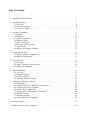
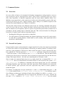
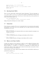
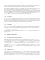
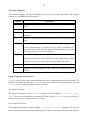
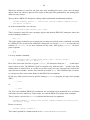
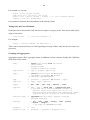
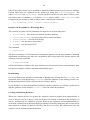
spatial or spatio-temporal data residing in files. All three components can be used together in a
configuration shown in Figure 1.
GUI
Optimizer
SECONDO Kernel
Figure 1: Cooperation of SECONDO Components
In this configuration, the GUI can ask the kernel directly to execute commands and queries (queries written as query plans, i.e., terms of the implemented algebras). Or it can call the optimizer to
get a plan for a given SQL query. The optimizer when necessary calls the SECONDO kernel to get
information about relation schemas, cardinalities of relations, and selectivity of predicates. Here
the optimizer acts as a server for the GUI and as a client to the kernel.
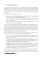
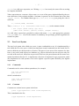
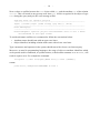
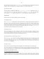
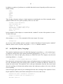
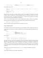
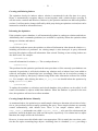
A very rough description of the architecture of the SECONDO kernel is shown in Figure 2. A data
model is implemented as a set of data types and operations. These are grouped into algebras.
Command Manager
Query Processor & Catalog
Alg1
Alg2
Algn
Storage Manager & Tools
Figure 2: Rough architecture of the kernel
The definition of algebras is based on the concept of second-order signature [Gü93]. The idea is
to use two coupled signatures. Any signature provides sorts and operations. Here in the first signature the sorts are called kinds and represent collections of types. The operations of this signature are type constructors. The signature defines how type constructors can be applied to given
types. The available types in the system are exactly the terms of this signature.
The second signature defines operations over the types of the first signature.
An algebra module provides a collection of type constructors, implementing a data structure for
each of them. A small set of support functions is needed to register a type constructor within an
algebra. Similarly, the algebra module offers operators, implementing support functions for them
such as type mapping, evaluation, resolution of overloading, etc.
The query processor evaluates queries by building an operator tree and then traversing it, calling
operator implementations from the algebras. The framework allows algebra operations to have
parameter functions and to handle streams. More details can be found in [DG00].
–
3
–
The SECONDO kernel manages databases. A database is a set of SECONDO objects. A SECONDO
object is a triple of the form (name, type, value) where type is a type term of the implemented
algebras and value a value of this type. Databases can be created, deleted, opened, closed,
exported to and imported from files. In files they are represented as nested lists (like in LISP) in a
text format.
Currently there exist about thirty algebras implemented within SECONDO. All algebras include
appropriate operations. Some examples are:
• StandardAlgebra. Provides data types int, real, bool, string.
• RelationAlgebra. Relations with all operations needed to implement an SQL-like relational
language.
• BTreeAlgebra. B-Trees.
• RTreeAlgebra. R-Trees.
• SpatialAlgebra. Spatial data types point, points, line, region.
• DateAlgebra. A small algebra providing a date type.
• MidiAlgebra. Providing a data type to represent the contents of Midi files including interesting operations like searching for a particular sequence of keys.
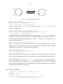
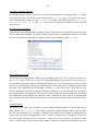
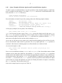
As a conclusion of this introduction, an example is shown in order to demonstrate how SECONDO
can be used to formulate queries on spatial objects. This example involves some objects in the
open database: (i) a relation Kreis with type (schema) rel(tuple([KName: string, ...,
Gebiet: region])) containing the regions of 439 counties (“Kreise”) in Germany, (ii) an object
magdeburg of type region, containing the geometry of county “Magdeburg”, and (iii) an object
kreis_Gebiet of type rtree(tuple([KName: string, ..., Gebiet: region])) which is an
R-tree on the Gebiet attribute of relation Kreis.
The following query finds neighbour counties of magdeburg:
query kreis_Gebiet Kreis
windowintersects[bbox(magdeburg)]
filter[.Gebiet adjacent magdeburg]
project[KName] consume
The query uses the R-tree index to find tuples for which the bounding box (MBR) of the Gebiet
attribute overlaps with the bounding box of the magdeburg region. The qualifying stream of
tuples is filtered by the condition that the region of the tuple is adjacent to the region of magdeburg. Tuples are then projected on their KName attribute and the stream is collected into a result
relation.
The following sections of this manual describe the use of SECONDO in detail.
–
4
–
2 Command Syntax
2.1 Overview
SECONDO offers a fixed set of commands for database management, catalog inquiries, access to
types and objects, queries, and transaction control. Some of these commands require type expression, value expression, or identifier arguments (used for object names, database names, etc.).
Whether a type expression or value expression is valid or not is determined by means of the specifications provided by the active algebra modules, while validity of an identifier depends on the
content of the actual database (see Chapter 3 for details).
The SECONDO kernel accepts two different syntax levels for entering commands and queries:
nested list syntax and text syntax. Nested list syntax is directly processed by the SECONDO kernel,
and it is uniform over all operators. However, queries in nested list syntax tend to contain a lot of
parentheses, thereby getting hard to formulate and read. This is the motivation for offering the
second level of query syntax with two important features:
• Reading and writing type expressions is simplified.
• For each operator of an algebra module, the algebra implementor can specify syntax properties like infix or postfix notation. If this feature is used carefully, value expressions can be
much more understandable.
2.2 Nested List Syntax
Using nested list syntax, each command is a single nested list. For short, the textual representation
of a nested list consists of a left parenthesis, followed by an arbitrary number of elements, terminated by a right parenthesis. Elements are either nested lists again or atomic elements like numbers, symbols, etc. The list expression (a b ((c)(d e))) represents a nested list of 3 elements:
a is the first element, b is the second one, and ((c)(d e)) is the third one. Thus the third element
of the top-level list in turn is a nested list. Its two elements are again nested lists, the first one consisting of the single element c, the other one containing the two elements d and e.
Since a single user command must be given as a single nested list, a command like list type
constructors has to be transformed to a nested list before it can be passed to the system: (list
type constructors). In addition to commands with fixed contents, there are also commands
containing identifiers, type expressions, and value expressions. While identifiers are restricted to
be atomic symbols, type expressions and value expressions may either be atomic symbols or
nested lists again.
For instance, assuming there are type constructors rel and tuple and attribute data types int and
string, the nested list term (rel (tuple ((name string)(pop int)))) is a valid type expression, defining a relation type consisting of tuples whose attributes are called name of type string
and pop of type int. Additionally SECONDO supports the definition of new types. Consider the
new type cityrel defined as (rel (tuple ((name string)(pop int)))): now the symbol
–
5
–
is a valid type expression, too. Writing cityrel has exactly the same effect as writing
its complete definition.
cityrel
Value expressions are constants, object names, or terms of the query algebra defined by the current collection of active algebra modules. Constants, in general, are two-element lists of the form
(<type> <value>). For standard data types (int, real, bool, string) just giving the value is
sufficient:
17, 3.14159, TRUE, "Secondo"
Thus, 5, cities, (+ 4 5), (count(head (feed cities) 4)), or the constant relation
( (rel (tuple ((name string) (pop int)))
(("New York" 7322000) ("Paris" 2175000) ("Hagen" 212000)))
are valid value expressions (provided an object with name cities and appropriate operators
feed, head and count exist. Prefix notation is mandatory for specifying operator application in
nested list syntax.
2.3
User Level Syntax
The user level syntax, also called text syntax, is more comfortable to use. It is implemented by a
tool called the SECONDO parser which just transforms textual commands into the nested list format in which they are then passed to execution. This parser is not aware of the contents of a database; so any errors with respect to a database (e.g. objects referred to do not exist) are only discovered at the next level, when lists are processed. However, the parser knows the SECONDO commands described in Section 2.3; it implements a fixed set of notations for type expressions, and it
also implements for each operator of an active algebra a specific syntax defined by the algebra
implementor.
2.3.1
Commands
Commands can be written without parentheses, for example
list type constructors
query cities
which is translated to
(list type constructors)
(query cities)
2.3.2
Constants
Constants are written in text syntax in the form
[const <type expression> value <value expression>]
This is translated to the list
(<type expression> <value expression>)
–
6
–
which is the list form of constants explained above. Of course, simple constants for integers etc.
can be written directly. For example,
[const
[const
[const
[const
int value 5] or 5
string value "secondo"] or "secondo"
bool value TRUE] or TRUE
rectangle value (12.0 16.0 2.5 50.0)]
might be notations for constants.
2.3.3
Type Expressions
Type constructors can be written in prefix notation, that is
<type constructor>(<arg_1>, ..., <arg_n>)
This is translated into the nested list format
(<type constructor> <arg_1> ... <arg_n>)
An example type expression is
rel(tuple([name: string, pop: int]))
This example uses notations for lists and pairs, which are translated by the parser as follows
[elem_1, ..., elem_n] -> (elem_1, ..., elem_n)
x: y -> (x y)
translated by the parser into
(elem_1 ... elem_n)
(x y)
So the expression rel(tuple([name: string, pop: int])) is transformed into the nested list
form shown in Section 2.2. The relation constant can now be written as
[const rel(tuple([name: string, pop: int]))
value (("New York" 7322000) ("Paris" 2175000) ("Hagen" 212000))]
2.3.4
Value Expressions
Value expressions are terms consisting of operator applications to database objects or constants.
For each operator a specific syntax can be defined. The parser is built at compile time taking these
specifications into account. The syntax for an operator can be looked up in a running system by
one of the commands
list operators
list algebra <algebra name>
These commands provide further information such as the meaning of the operator. For example,
the entry appearing on list operators for the operator year_of is
–
Name:
Signature:
Syntax:
Meaning:
Example:
7
–
year_of
instant -> int
year_of ( _ )
return the year of this instant
query year_of(T1)
This specifies prefix syntax for the operator year_of. Be aware that what appears in such a listing
is a comment written by the algebra implementor which occasionally may be wrong. More details
on the specification of an operator can be found in the SECONDO Programmer’s Guide.
Parameter Functions
The following operator demonstrates another general concept for query formulation: anonymous
function definition. Its main purpose is to define predicate functions for operators like filter,
taking a stream of tuples and a boolean function as parameters1. The function is applied to each
tuple and filter lets the tuple pass if the function returns true.
filter [fun (tuple1: TUPLE) attr(tuple1, no) > 5]
In this example, fun is the keyword for the function, tuple1 is the name which is assigned to the
current tuple of the stream. By using this name, a tuple can be accessed. attr is an operator which
extracts from the tuple passed as first argument the value of the attribute whose name is given in
the second argument. Finally, the > operator is the binary infix operator which returns a boolean
value that decides whether the tuple is passed through or not. For the given example, on a relation
with an attribute no that contains numbers, the filter expression lets pass all tuples which have
a no attribute with a value greater than 5.
However, this expression is a bit lengthy to write. For parameter functions, SECONDO allows one
to use an abbreviated form. When using this form, a variable name and the correct type are generated automatically. This allows one to write the expression above as follows:
filter [attr(., no) > 5]
The parser translates this to the form shown above (and translates it then to the appropriate nested
list form). Of course, when writing the expression one does not know which parameter name is
generated by the parser (in particular, the parser assigns distinct numbers); hence there must be
another way to refer to it, and that is the “.” symbol. The same mechanism is available for operators with parameter functions taking two arguments (e.g. for implementing join operators referring to the tuple types of the first and the second argument separately, i.e. two input streams); in
that case the symbol “..” can be used to refer to the second argument. Instead of the symbol “.”
one can also write tuple or group as this makes sense for many operators; it is translated by the
parser in the same way as the “.” symbol.
Finally, attribute access is very frequently needed, therefore notations
.<attrname>
..<attrname>
are provided equivalent to the expressions
1. How a stream of tuples is created from a relation will be the subject of the subsequent chapter.
–
8
–
attr(., <attrname>)
attr(.., <attrname>)
So the use of the attr operator has been hard-coded into the parser. Finally, we can write the
application of filter as
filter [.no > 5]
–
9
–
3 SECONDO Commands
There is a fixed set of commands implemented at the SECONDO application programming interface. These commands can be called from one of the user interfaces described in Section 5. An
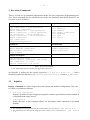
overview is given in Table 1.
Basic Commands
Inquiries
type <identifier> = <type expression>a
delete type <identifier>
create <identifier> : <type expression>
update <identifier> := <value expression>
let <identifier> = <value expression>
derive <identifier> = <value expression>
delete <identifier>
kill <identifier>
query <value expression>
list
list
list
list
list
list
list
Databases
Transactions
create database <identifier>
delete database <identifier>
open database <identifier>
close database
begin transaction
commit transaction
abort transaction
type constructors
operators
algebras
algebra <identifier>
databases
types
objects
Import and Export
save database to <file>
restore database <identifier> from <file>
save <identifier> to <file>
restore <identifier> from <file>
Table 1: SECONDO Commands
a.User defined data types are currently not supported by the kernel.
An identifier is defined by the regular expression [a-z,A-Z]([a-z,A-Z]|[0-9]|_)* with a
maximal length of 48 characters, e.g. lineitem, employee, cities_pop but not _x_ or 10times.
3.1
Inquiries
Inquiry commands are used to inspect the actual system and database configuration. They can
be called even without a database.
•
list type constructors
Displays all names of type constructors together with their specification and an example in
a formatted mode on the screen.1
•
list operators
Nearly the same as the command above, but information about operations is presented
instead.2
1. The information can also queried using the system relation SEC2TYPEINFO (see Section 3.6)
2. The information can also queried using the system relation SEC2OPERATORINFO (see Section
3.6).
–
•
10
–
list algebras
Displays a list containing all names of active algebra modules.
•
list algebra <identifier>
Displays type constructors and operators of the specified algebra.
• list databases
Displays a list of names for all known databases.
• list types3
Displays a list of type names defined in the currently opened database.
• list objects
Displays a list of objects present in the currently opened database.
3.2
Databases
Database commands are used to manage entire databases.
•
create database <identifier>
Creates a new database. A database name may have only up to 15 characters and no
distinction between uppercase and lowercase letters is made.
•
delete database <identifier>
Destroys the database <identifier>.
•
open database <identifier>
Opens the database <identifier>.
• close database
Closes the currently open database.
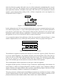
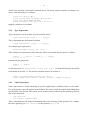
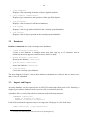
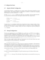
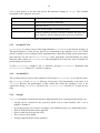
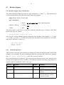
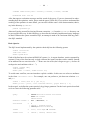
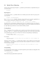
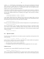
The state diagram in Figure 3 shows how database commands are related to the two states OPEN
and CLOSED of a database.
3.3
Import and Export
An entire database can be exported into an ASCII file and loaded from such a file. Similarly, a
single object within a database can be saved to a file or restored from a file.
A database file is a nested list with four elements of the following structure:
(DATABASE <identifier>
(TYPES <a sequence of types>)
(OBJECTS <a sequence of objects>))
Each of the mentioned sequences may be an empty list. Each type is a list of the form
(TYPE <identifier> (<type expression>))
3. Currently, user defined types cannot be used in any meaningful way.
–
11
–
and each object is a list of length five with the following structure
(OBJECT <identifier>
(<type identifier>)
(<type expression>)
(<value expression>))
An object does not need to have a named type. In that case the third element is an empty list. A
file storing a single object contains only one object list.
•
save database to <file>
Write the entire contents of the currently open database in nested list format into the file
<file>. If the file exists, it will be overwritten, otherwise it will be created.
•
restore database <identifier> from <file>
Read the contents of the file <file> into the database <identifier>.
Previous contents of
the database are lost. If the database is not yet present, it will be created.
•
save <identifier> to <file>
Writes the object list for object <identifier>
to file <file>. The content of an existing
file will be deleted.
•
restore <identifier> from <file>
Creates a new object with name <identifier>,
possibly replacing a previous definition.
Type and value of the object are read from file <file>.
In the commands above a <file> can be an identifier or a nested list text atom which can hold
character sequences of arbitrary length and is recognized by the nested list parser by enclosing it
with the tags <text> and </text---> or in single quotes. Moreover, it is possible to use environment variables. Examples:
save cities to cities_obj
save cities to ’$(HOME)/cities.obj’
save cities to <text>/media/usb/memorystick/cities.obj<text--->
On a MS-Windows system you have to use the backslash as directory separator, e.g.
save database to ’C:\msys\mydb.db’
3.4
Database States
Figure 3 shows how commands depend on and change the state of a database. The commands
referred to all have the keyword database in their syntax. All commands accessing objects only
work in an open database.
3.5
Basic Commands
These are the fundamental commands executed by SECONDO. They provide creation and manipulation of types and objects as well as querying, within an open database.
•
type <identifier> = <type expression>
Creates a new type named <identifier> for the
given type expression.
–
create
12
–
open, restore
CLOSED
save
OPEN
close
delete
Figure 3: Database Commands and States
•
delete type <identifier>
Deletes the user defined type named <identifier>.
•
create <identifier> : <type expression>
Creates an object called <identifier> of the type
given by <type expression>. The
value is still undefined.
•
update <identifier> := <value expression>
Assigns the result value of the right hand side to the object <identifier>.
•
let <identifier> = <value expression>
Assign the result value right hand side to a new object called <identifier>. The object is
not allowed to exist yet; it is created by this command and its type is defined as the one of
the value expression. The main advantage vs. using create and update is that the type is
determined automatically.
•
derive <identifier> = <value expression>
This is a variant of the let command which can be useful to construct objects which use
other objects as input and have no external list representation, e.g. indexes. When restoring
a database those objects are reconstructed automatically.
•
delete <identifier>
Destroys the object whose name is <identifier>.
•
query <value expression>
Evaluates the given value expression and returns the result object. If the user interface provides no special display functions for the object’s type it will be displayed as a nested list.
•
kill <identifier>
Removes the object whose name is <identifier> from the database catalog without removing its datastructures. Generally, the delete command should be used to remove database
objects, but this command may be useful if delete would crash the database due to corrupted
persistent data structures for this object.
Some example commands:
type myrel = rel(tuple([Name: string, Age: int]))
create x : int
update x := 5
let place = “Hagen“
let rel2 = [const rel(tuple([Name: string, Age: int]))
value ((“Peter“ 17)(“Klaus“ 31))]
–
13
–
derive rel2_Age = rel2 createbtree[Age]
query (x * 7) + 5
query rel2 feed filter[.Age > 20] project[Name] consume
delete type myrel
delete rel2
3.6
Querying System Tables
There are some system tables which provide internal information. The most interesting are
SEC2COMMANDS and SEC2OPERATORINFO. The first one contains a command history and the second
contains descriptions of the operators. Since they are relation objects they can by queried by the
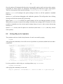
means of the relational algebra, e.g.
query SEC2OPERATORINFO feed
filter[.Signature contains "stream(tuple"] consume
displays all operators which process a stream of tuples.
3.7
Transactions
Each of the basic commands of SECONDO is encapsulated into its own transaction and committed
automatically. If you want to put several commands into one single transaction the following
commands have to be used.
• begin transaction
Starts a new transaction; all commands until the next commit command are managed as one
common unit of work.
• commit transaction
Commits a running transaction; all changes to the database will be effective.
• abort transaction
Aborts a running transaction; all changes to the database will be revoked.
3.8
Hints to avoid Name Conflicts
Currently, the optimizer uses the underscore symbol to encode additional information about
objects into their names; for example, an object named myrel_Attr will be considered to be an
index for attribute Attr in relation myrel. Therefore we recommend to use attribute names and
relation names which are short enough, since the name of an index object can only have 48 characters and to avoid usage of the underscore.
Another problem can be name conflicts between database objects and identifiers which may be
parameters for operators, e.g.:
let pop = FALSE;
query cities feed project[pop] consume
–
14
–
Now we have a conflict between the bool object called pop and the attribute pop of the relation
citites. This will result in an type map error since pop will be recognized as an object of type
bool during the query analysis, the error message will be
Type map error for operator project!
---------------------------------------------------------------------Input: ((stream (tuple ((name string) (pop int)))) (bool))
---------------------------------------------------------------------Error Message(s):
---------------------------------------------------------------------RelationAlgebra: Operator project: Attributename 'bool' is not a known
attributename in the tuple stream.
To avoid such name conflicts we recommend to follow the conventions below:
• Attribute names should start with an upper case letter.
• Object identifers including relation names start with a lower case letter.
Type constructors and operators in the system should start with a lower case letter anyway.
Moreover, as usual in programming languages, the usage of object or attribute identifiers which
are keywords used in commands, or operator names, or the boolean constants TRUE or FALSE, will
result in a parse error. For example the command
let myrel1 = [const rel(tuple([TRUE: bool])) value ((FALSE))]
returns
parse error, unexpected ZZBOOLEAN in line 1
–
15
–
4 Configuration Issues
4.1
Algebra Module Configuration
As described in Section 1, a running SECONDO system consists of the kernel extended by several
algebra modules. These algebra modules can arbitrarily be included or excluded when compiling
and linking the system by running the make utility.
The file makefile.algebras contains two entries for every algebra. The first defines the directory name and the second the name of the algebra module like in the example below:
...
ALGEBRA_DIRS += Polygon
ALGEBRAS
+= PolygonAlgebra
ALGEBRA_DIRS += BTree
ALGEBRAS
+= BTreeAlgebra
...
Currently, there is no mechanism which detects dependencies between algebra modules. Hence
read the comments in the file. In case of trouble you have to switch on or off more algebras than
the single one you wanted to change. Finally you need to recompile the system by calling the
make command.
4.2
Startup Configuration
The SECONDO applications SECONDOTTYBDB, SECONDOPL, SECONDOTTYCS, SECONDOMONITOR will read their configuration parameters from a file called SecondoConfig.ini which is
searched for in the current directory. Optionally, if the environment variable SECONDO_CONFIG is
defined, its value will be used as an absolute file name for the configuration file instead. On most
installations this will be already defined as $HOME/secondo/bin/SecondoConfig.ini.
There are many possible options which are documented in the file itself, hence only some
important options will be mentioned here. The parameter
SecondoHome=/home/databases1
defines the node in the directory tree where SECONDO could store its databases. If this parameter
is not defined or if it points to a non-existing directory the directory $HOME/secondo-databases
is used. When you plan to restore big databases, you should switch off the usage of transactions,
since otherwise mega- or giga-bytes of log files – Berkeley-DB does physical logging after each
write operation on a page – are written to disk. This can be done by uncommenting the line
RTFlags += SMI:NoTransactions
If you have already produced gigabytes of log files and want to get rid of them, call the script
rmlogs
in the secondo/bin directory. This will delete all log files that are not needed for recovery any
more.
–
16
–
5 User Interfaces
5.1
Overview
SECONDO comes with five different user interfaces, SecondoTTYBDB, SecondoTTYCS, SecondoPL,
SecondoPLCS and Javagui. For testing, a further programm named TestRunner is available. The
shell-based interfaces without optimizer support can be found in the bin directory. All programs
related to the optimizer are in the Optimizer directory. Javagui is located in the Javagui directory.
SecondoTTYBDB is a simple single-user textual interface, implemented in C++. It is directly linked
with the system frame. It is mainly used for debugging and testing the system without relying on
client-server communication. SecondoPL is the single-user version of the optimizer. SecondoTTYCS, SecondoPLCS and Javagui are multi-user client-server interfaces. They exchange messages with the system frame running as a server process via TCP/IP. Provided that the database
server process has been started, multiple user interface clients can access a SECONDO database
concurrently.
5.2
5.2.1
Single-Threaded User Interfaces
SecondoTTYBDB
is a straightforward interface implementation. Both, input and output are textual.
Since SecondoTTYBDB materializes in the shell window from which it has been started, existence
and usage of features like scrolling, cut, copy and paste etc. depend on the shell and window manager environment. A command ends with a “;” or an empty line. Thus, multi-line commands are
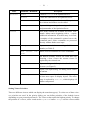
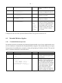
possible. SecondoTTYBDB provides some special commands described in the following table:
SecondoTTYBDB
Command
Description
? or HELP
Displays all user interface commands.
@<filename>
Starts batch processing of the specified file. The file must be in the
bin directory. All lines are subsequently passed to the system, just as
if they were typed in manually by the user. After the last command
line was executed, SecondoTTYBDB returns to the interactive mode.
DEBUG {0|1|2}
Sets the debug mode. See online help for further information.
q or quit
Quits the session. A final abort transaction is executed automatically. After that, SecondoTTYBDB is terminated.
Table 2: Commands of SecondoTTYBDB
For the algebra modules, SecondoTTYBDB is extended by support functions for pretty printed output of tuples and relations. Note that the implementation of these functions is optional. As a con-
–
17
–
sequence, there might be algebra modules having types for which no pretty printing can be performed. In this case, objects having such a type are displayed in nested list format.
If the readline functionality is enabled (see Installation Guide), some additional features are available: The command history can be stepwise passed by pressing the cursor-up and cursor-down
keys, respectively. The history remains available even after termination of SECONDO. By pressing
the tab key, the input is extended to the next matching keyword. Keywords are all words from the
SECONDO commands (list, database, etc.) and some frequently used operators (feed, consume). A double tab prints out all possible extensions of the current word.
5.2.2
SecondoPL
is the text-based interface of the SECONDO optimizer. To start this interface, navigate
into the Optimizer directory of SECONDO and enter SecondoPL. At the first run of SecondoPL
some error messages regarding non-existing files are shown. They can be ignored. On Linux
machines you will have the advantages of the readline library if it is installed.
SecondoPL
5.2.3
TestRunner
The TestRunner can be used for automatic testing of operators including checks for the correct
(expected) results. For using the TestRunner, navigate into SECONDO’s bin directory and enter
TestRunner -i <inputfile>
The format of the inputfile is described in the file example.test which is located in the bin
directory as well.
5.3
5.3.1
Multi-User Operation
SecondoMonitor and SecondoListener
Before the client-server user interfaces can be used, the database server process (SecondoListener)waiting for client requests must be started. The host name and the port address can be
changed in the file SecondoConfig.ini. Start the SecondoListener by typing SecondoMonitor. At the prompt, startup should be entered. By using the -s option with the SecondoMonitor
command, the SecondoListener is started automatically without the additional startup command. After SecondoListener is started, it waits for requests from clients. HELP shows a list of
additional commands.
5.3.2
OptimizerServer
If one intends to use the optimizer within Javagui, also an optimizer server has to be started.
Because this server acts as a client for SECONDO, the SecondoListener has to be started before
executing the optimizer server. To start the optimizer server, navigate into the Optimizer directory of SECONDO and enter StartOptServer [Port]. Without any argument, the default port
–
18
–
1235 is used. Ensure to use the same port in the optimizer settings of Javagui. The available
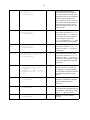
commands of the optimizer server are:
Command
Description
help
Prints out the available commands.
quit
Quits the server.
clients
Prints out the number of connected clients.
trace-on, trace-off
Enables (disables) tracing. If tracing is enabled, the query, the
used database and the computed query plan are printed out.
Table 3: Commands of the optimizer server
5.3.3
SecondoTTYCS
SecondoTTYCS is a client version of the single-threaded SecondoTTYBDB described in Section 5.2.
The main difference is that all user queries are transmitted to the database server via TCP/IP,
which is capable to serve multiple clients simultaneously, rather than calling system frame procedures directly. For the user of a SecondoTTYCS client, appearance and functionality are pretty
much the same as those of SecondoTTYBDB. All commands work in the same way as with the single-threaded user interface.
To start SecondoTTYCS, change to the bin directory, and type SecondoTTYCS. Remember that
SecondoListener (Section 5.3.1) must be running.
5.3.4
SecondoPLCS
The text-based client version of the optimizer of SECONDO is SecondoPLCS. It is started by entering SecondoPLCS in the Optimizer directory of SECONDO. The functionality is the same as in
SecondoPL. Because the optimization is done within this client, the optimizer server is not
required for using SecondoPLCS. However, the SecondoListener (Section 5.3.1) must be running.
5.3.5
Javagui
Javagui
is a window-oriented user interface implemented in Java. Among its main features are:
• Javagui can be executed in any system in which a Java virtual machine (Ver. 1.4.2 or
higher) is installed.
• It provides a large set of viewers to display a lot of different types (e.g. spatial data types).
• Data of different formats can be imported.
• Query results can be saved into a file.
• New viewers can be added.
• Javagui supports the SECONDO optimizer.
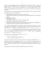
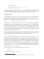
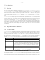
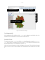
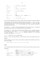
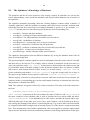
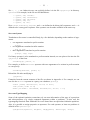
Command Panel
19
–
Object Manager
Current Viewer
Progress Bar
–
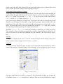
Figure 4: The four Parts of Javagui
The Configuration File
In the configuration file, variables used by Javagui can be changed to non-default values. In a
standard SECONDO installation it is not necessary to change this file.
Starting the Javagui
The easiest way to start Javagui is to call the sgui script. Remember to start the SecondoListener process before executing the script (see Section 5.3.1). For optimizer functionality, ensure
that the OptimizerServer is also running (see Section 5.3.2).
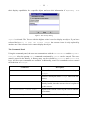
After some licence information, a window will appear on the screen. This window has four main
parts: the current viewer, the object manager, the command panel, and a progress bar (see Figure
4).
–
20
–
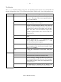
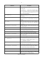
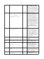
The Menubar
The Javagui menubar consists of two parts: one depending on the current viewer and another one
which is independent from it. The following description includes only viewer-independent parts.
Menu
Program
Server
Submenu / Menuitem
Description
New
Clears the history and removes all objects from
Javagui. The state of SECONDO (opened databases
etc.) is not changed.
Fontsize
Here, the fontsize of the command panel and
object manager can be changed.
Execute File
Opens a file input dialog to choose a file. Then the
batch mode is started to process the content of the
selected file. It can be chosen how errors are handled. Note, there exist two different script styles
which are described and can be selected in the configuration file.
History
In this menu the current history can be manipulated.
Snapshot
Stores a Picture of the Javagui window into a file
as png image. The key combination <alt C> can
also be used to make a snapshot.
Screen snapshot
Works similar to the Snapshot menu entry but creates a snapshot of the whole screen instead of only
the Javagui window.
Exit
Closes the connection to SECONDO and quits
Javagui.
Connect
Connects Javagui to SECONDO.
Disconnect
Disconnects the user interface from SECONDO.
Settings
Shows a dialog to change the address and port used
for communication with SECONDO. For a permanent change of these values, the configuration file
should be used.
User settings
If authorization is enabled (off by default), the
username and the password can be entered here.
Table 4: Menubar of Javagui
–
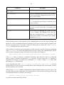
Menu
Optimizer
Viewers
–
Submenu / Menuitem
Description
Enable
Connects Javagui to an OptimizerServer.
Disable
Closes the connection to an OptimizerServer.
Command
In this menu, the update functions of the optimizer
for relations and indexes can be called.
Settings
Opens a dialog to change the settings of hostname
and portnumber of the OptimizerServer.
This menu contains all available SECONDO commands. Menu entries beginning with a ~ require
additional information. If such an entry is selected,
a template of the command is printed out to the
command panel. Other commands are processed
directly without further user input.
Command
Help
21
Show gui commands
Opens a new window containing all Gui commands (see Table 5).
Show secondo
mands
Shows a list of all known SECONDO commands.
com-
<name list>
All known (loaded) viewers are listed here. By
choosing a new viewer the current viewer is
replaced by the selected one.
Set priorities
Opens a dialog to define priorities for the loaded
viewers (see Figure 5).
Add Viewer
Opens a file input dialog for adding a new viewer
at runtime.
Show only viewer
Hides the command panel and the object manager
to have more space to display objects. The menu
entry is replaced by show all, which displays all
hidden components.
Table 4: Menubar of Javagui
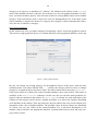
Setting Viewer Priorities
There are different viewers which can display the same data type(s). To select one of these viewers, priorities are used. In the priority dialog you can define priorities of the loaded viewers
depending on your personal preferences. The viewer at the top has the highest priority. To change
the position of a viewer, select it and use the up or down button. Javagui ask the viewers about
–
22
–
their display capabilities for a specific object and uses this information if depending from
Figure 5: The Priority Dialog
is selected. The Viewer with the highest value is used to display an object. If you have
selected the box try to keep the current viewer, the current viewer is only replaced by
another one if the current viewer cannot display the object.
object
The Command Panel
Using the command panel, the user can communicate with the SecondoServer and the OptimizerServer. After the prompt Sec>, commands terminated by return can be entered. The command is stored in the history. A history entry can be selected by cursor-up and cursor-down
keys. All SECONDO commands are available. Additionally, some Gui commands exist to control
the behaviour of Javagui:
Command
Description
gui exit
Closes the connection to SECONDO and quits
Javagui.
gui clearAll
Removes all objects from Javagui and clears the
history.
gui addViewer <viewer name>
Adds a new viewer at runtime. If the viewer was
already loaded, then the current viewer is replaced
by this viewer.
gui selectViewer <viewer name>
Replaces the current viewer by the viewer with the
given name.
gui clearHistory
Removes all entries from the history.
Table 5: Gui Commands
–
23
–
Command
gui loadHistory [-r]
Description
Shows a file input dialog and reads the history
from this file.
Used with the -r option this command replaces
the current history with the file content. Without
the -r option this command appends the file content to the current history.
gui saveHistory
Opens a file dialog to save the content of the current history.
gui showObject <ObjectName>
Shows an object from the object manager in a
viewer. The viewer is determined by the priority
settings.
gui showAll
Shows all objects listed in the object manager in
the current viewer, whose types are supported by
this viewer.
gui hideObject <ObjectName>
Removes the object with the specified name from
the current viewer.
gui hideAll
Removes all objects from the current viewer.
gui removeObject <ObjectName>
Removes the object with the given name from the
object manager and from all viewers.
gui clearObjectList
Removes all objects from the object manager.
gui saveObject <ObjectName>
Opens a file dialog to save the object with the
given object name.
gui loadObject
Opens a file dialog to load an object.
gui setObjectDirectory
<directory>
Sets the object directory.
This directory is initially shown when a load or
save command is executed.
gui loadObjectFrom <Filename>
Loads the object with the specified filename.
The file must be located in the objectdirectory.
gui storeObject <ObjectName>
Stores an object into the currently open database.
The object name must not contain spaces.
gui connect
Connects Javagui to SECONDO.
gui disconnect
Disconnects Javagui from SECONDO.
gui serverSettings
Opens the server setting dialog to change the
default settings for host name and port.
Table 5: Gui Commands
–
24
–
Command
Description
gui renameObject <old name> ->
<new name>
Renames an object.
gui onlyViewer
Hides the command panel and the object manager.
To show the hidden components use the Viewers
entry in the menubar.
gui executeFile [-i] <filename>
Batch processing of the file.
If -i is set then file processing is continued even if
an error occured.
gui status
Prints out information about the connection to
SECONDO as well as the name of currently open
database.
gui set
Can be used for changing the values of some
Javagui settings. The complete list of the variables can be obtained by the help menu entry. The
effect of the variables is described in the configuration file of Javagui.
Table 5: Gui Commands
Each non-empty query result requested in the command panel is sent to the object manager and
shown in a viewer according to the priority settings. If no viewer is found, which is capable to display the requested object, a message is shown to inform the user about this. If the StandardViewer is loaded, this case will never occur.
If the optimizer is enabled, queries and updates in SQL syntax are possible. All queries beginning
with select or sql are send to the OptimizerServer to get a query plan. Embedded SQL queries
can be used for a postprocessing of the result of such a query. An example is
query (select sname from staedte where bev>500000) feed head[3] consume
Each select-clause in brackets is optimized separately. Note that the result of an optimized
query is always a relation (exceptions are count queries). For this reason, the feed operator is
required in the example. In contrast to an embedded select-clause, a single select-clause adds
the leading query automatically.
If the command starts with insert into, delete from, or update <identifier> set, also the
OptimizerServer is used to get an executable plan for that command. The received plan is sent to
the SecondoServer for execution.
The keyword optimizer enables communication with the OptimizerServer at a lower level. The
text after this keyword is transfered to the OptimizerServer, converted into a Prolog predicate and
evaluated afterwards. For example, you can type
optimizer current_prolog_flag(version, Version)
to get the currently used Prolog version.
–
25
–
The Object Manager
This window manages all objects resulting from queries or file input operations. The manager
provides a set of buttons described below:
Button
Description
show
Shows the selected object in the viewer depending on priority settings.
hide
Removes the selected object from the current viewer.
remove
Removes the selected object from all viewers and from the object
manager.
clear
Removes all objects from all viewers and also from the object manager.
save
Opens a file dialog to save the selected object to a file.
If the selected object is a valid SECONDO object [consisting of a
nested list (type value)] and the chosen file name ends with obj then
the object is saved as a SECONDO object.
load
Opens a file dialog to load an object.
Supported file formats are nested list files, shape files or dbase3 files.
In the current version, restrictions for shape and dbf files exist.
store
Stores the selected object into the currently open database.
rename
Replaces the object manager with a dialog to rename the selected
object.
Using Javagui for Test Purposes
can be used to make tests including client server communication and the optimizer. The
different test modes provided by Javagui are presented in this section. Remember to start the
SecondoListener and the optimizer server if needed.
Javagui
The Simple Test Mode
The simple test mode is used if Javagui is started with the option(s) --testmode [<filename>]. Here, all user interaction is switched off. If the optional filename is given, it will be executed, as if a script is executed via the file menu.
The Extended Test Mode
The extended test mode is started using the --testmode2 <filename> arguments. The test file
has to contain a nested list with the commands to execute as well as the expected results. The for-
–
26
–
mat is described in detail in the GuiTestmodes.pdf file which is part of a standard SECONDO distribution. After executing this file, Javagui will halt for 5 seconds and then exit.
The Testrunner Mode
This test mode is enabled by adding the --testrunner <filename> arguments to the sgui
script. The file has to be in the same format as the TTY-based TestRunner files. The only difference is that in Javagui testfiles also queries in SQL-like (Optimizer-) syntax are allowed.
The Viewers
In this section, some of the available viewers are presented.
The Standard Viewer
The StandardViewer simply shows a SECONDO object as a string representing the nested list of
this object. In the text area only one object is displayed at the same time. To show another object
in this viewer it must be selected in the combobox at the top of this viewer. You can remove the
current (or all) object(s) in the extension of the menubar. Make sure to load the StandardViewer
by default to be able to display any SECONDO object.
The Relation Viewer
This viewer displays SECONDO relations as a table. The relation that shall be displayed can be
selected in the combobox at the top of this viewer. The viewer is not suitable for displaying relations with many attributes or relations containing large objects.
The Formatted Viewer and the Inquiry Viewer
The Formatted Viewer shows the results of inquiries sent to SECONDO in a similar way as the
SecondoTTY does. The Inquiry Viewer shows objects of the same types as a colorized table. In
the default configuration file, this viewer is not included. It has to be loaded first by using by the
gui addViewer command.
The Hoese Viewer
This viewer is very powerful and is able to display a lot of different SECONDO object types.
The viewer consists of several different parts to display textual, graphical and temporal data. If an
object in the textual part is selected, then the corresponding graphical representation is also
selected (if it exists) and vice versa.
The Textual Representation of an Object
Using the combobox at the top of the text panel you can choose another object (query result) to
display. A string in the text representation of the selected object can be searched by entering the
–
27
–
search string in the field at the bottom of the text panel and clicking on the go button. If the end of
text is reached, the search continues at the beginning of the text.
The Graphical Representation of Objects
The graphic panel contains geometric/spatial objects. Press the right mouse button and drag the
mouse holding the right mouse button for zoom in. Stepwise zoom in (zoom out) is available in
the Settings menu or by pressing Alt + (Alt -). To get an overview of all objects click on
Zoom out in the Settings menu or press Alt z.
Each query result is displayed in a single layer. Using layers, the order in which the objects are
displayed can be changed. To hide/show a layer use the green/gray buttons on the left of the
graphic panel. The order of the layers can be set in the layer management located in the Settings
menu. A selected object can be moved to another layer using the Object menu. Here, the user
also can change the display settings for a single selected object.
The menu Settings->Projections offers the possibility to enable one of a set of projections.
This is helpful, if data containing geographical coordinates (longitude, latitude) should be displayed. The usual view of such data is obtained using the Mercator or the Gauss-Krueger projection.
Sessions
A session is a snapshot of the viewer’s state. It contains all objects and the display settings. You
can save, load or start an empty session from the File menu.
Categories
A category contains information how an object is to be displayed. Such information is color or
texture of the interior, color and thickness of the borderline, or size and shape of a point. Catego-
Figure 6: Category Editor
ries can be loaded and saved via the File menu. To edit an exististing category, the category editor available via the Settings menu has to be invoked. There are several possibilities to assign a
–
28
–
category to an object or to attributes of a relation. The method can be chosen in the Settings
menu. If the manual selection is choosen, for each object (or for each graphical attribute of a relation), a selection window pops up. Auto selection creates for each graphical object a new random
category. If the selection by name is used, two cases are distinguished. First, if the name of the
object (attribute) is equal to the name of a category, this category is chosen automatically. Otherwise, the user is asked for a category.
Query Representation
In this window the user can make settings for displaying a query result with graphical content.
This can be a single graphical object or a relation with one or more graphical attributes. At the top
Figure 7: Query Representation
the user can choose an existing category for all graphical objects of this query with the same
(attribute) name. The button labeled with “...” invokes the category editor to create or change
categories. A graphical object may have a label. The label content can be entered as Label Text.
If the object is part of a relation, the value of another attribute can be used as label. This feature is
available in the Labelattribute combobox. In this case, the user can also make graphical settings for objects contained in the relation. If Single Tuple is selected, for each single tuple in the
relation an own category can be chosen. Another possibility is to choose the category depending
on an attribute in the relation. Thus, the point size, the line width or the color can be chosen to be
dependent on the value of another attribute. The possible values for these features are distributed
in a linear way over the values of the selected attribute. For a non-linear distribution or for
attribute values which do not support this function, a manual link between value and used category can be created.
–
29
–
Animating Temporal Objects
If a spatial-temporal object is loaded, you can start the animation by clicking on the play button
left of the time line. The speed can be chosen in the Settings menu. The speed can also be
halved (doubled) by clicking on the [<<]speed[>>] buttons. The other buttons are play, play
backwards, go start, go end and stop. You can also use the time scrollbar to select a desired
point in time.
Displaying Special Objects
Some objects can be displayed in a separate window. These objects are marked by a special color
in the textual representation. By double clicking on the object, an additional window is opened
and the selected object is displayed. Figure 8 shows such a window for the text type.
Figure 8: Special representation of the text type
Managing Backgrounds
The background of the graphic window can be changed by the user. The color can be chosen via
the Settings menu. This color is used if no background image is given and for all areas not covered by the background image. A background image can be used to show the context of other
objects. For positioning the image, the bounding box of this image must be defined together with
the image. For simplifying the positioning, so-called tfw files can be used. Such files are also
used in geographic information systems. Another possibility to set the background is to capture
the current display as background. This may be useful if many non-moving objects are displayed
and additional moving objects are animated. After capturing the static objects as background,
these objects can be removed from the display to reduce the computation effort during the animation.
Creating Objects
The HoeseViewer offers the possibility to create simple graphical objects. An object type can be
chosen in the Object Creation menu. After pressing the unlabeled button (right of the time line)
the object creation starts. For creating a rectangle, the rectangle can be drawn by holding the left
mouse button pressed and dragging the mouse. A point is created just by clicking on its location.
For the creation of other objects, a sequence of points has to be created by left mouse button
clicks. To finish the creation of such more complex objects, the object creation button has to be
–
30
–
pressed again. If an object is defined, it is stored into the currently open database and inserted into
the object manager.
–
31
–
6 Algebra Modules
6.1
Overview
Included in the full SECONDO release is a large set of different algebra modules. Three of these
algebras are somehow fundamental and therefore are described here in detail. They are:
• the standard algebra (StandardAlgebra in the algebra list)
• the relation algebra (RelationAlgebra in the algebra list)
• an extension to the relation algebra (ExtRelationAlgebra in the algebra list)
All three algebras are located in the Algebras-directory of the SECONDO installation. Algebra
modules can be activated and deactivated by changing the configuration of SECONDO
(makefile.algebras, see Section 4.1). However, the denoted three algebras are activated by
default.
6.2
6.2.1
Standard Algebra
Standard Type Constructors
The standard algebra module provides four constant type constructors (thus four types) for standard data types:
• int (for integer values): The domain is that of the int type implemented by the C++ compiler, typically -2147483648 to 2147483647 on 32-bit wide platforms.
• real (for floating point values): The domain is that of the float type implemented by the C++
compiler.
• bool: The value is either TRUE or FALSE.
• string: A value consisting of a sequence of up to 48 characters.
As all attribute types, these data types allow each value to be undefined. Thus, for instance, integer division by zero does not cause a runtime error, but the result is an undefined integer value.
6.2.2
Standard Operators
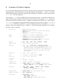
Table 6 shows the most important operators provided by the standard algebra module. Most of the
operations (like +, -, *, /) are overloaded and work for both types, int and real. For more information about specific operations type list algebra StandardAlgebra in your SECONDO interface.
In Table 6 we use the following notations. For signatures, an expression like int || real means
that either of the types int or real can be used as an argument. In the syntax column, “_” denotes
an argument, and “#” the operator; parentheses have to be put as shown.
–
32
–
Operator
Signature
Syntax
Semantics
+, -, *
int x int -> int
int x real -> real
real x int -> real
real x real -> real
_ # _
addition, subtraction, multiplication
/
(int || real) x (int || real) -> real
_ # _
division
div, mod
int x int -> int
_ # _
integer division and modulo
operation
<, <=,
>, >=,
=, #
(int || real) x (int || real) -> bool
string x string -> bool
_ # _
comparison operators
starts
string x string -> bool
_ # _
TRUE if arg1 begins with arg2
contains
string x string -> bool
_ # _
TRUE if arg1 contains arg2
not
bool -> bool
# ( _ )
logical not
and, or
bool x bool -> bool
_ # _
logical and
Table 6: Standard Operators
6.2.3
Query Examples (Standard Algebra)
Notice that queries can only be processed after a database was opened by the user. In the query
command
query <value expression>
is a term over the active algebra(s). Some examples for queries using the
standard algebra are given in Table 7. Note that no operator takes priority over another operator.
Therefore a multiplication is not computed before an addition as the examples 3 and 4 show. Parentheses must be used in this case.
value expression
Text Syntax
Nested List Syntax
query 5;
(query 5);
query 5.0 + 7;
(query (+ 5.0 7));
query 3 * 4 + 9;
(query (* 3 (+ 4 9)));
query (3 * 4) + 9;
(query (+ (* 3 4) 9));
query 6 < 8;
(query (< 6 8));
query (“Secondo” contains “cond”)
and TRUE;
(query
(and
(contains “Secondo” “cond”)
TRUE));
Table 7: Query Examples (Standard Algebra)
–
6.3
33
–
Relation Algebra
6.3.1 Relation Algebra Type Constructors
The relational algebra module provides two type constructors rel and tuple. The structural part
of the relational model can be described by the following signature:
kinds IDENT, DATA, TUPLE, REL
type constructors
→ DATA
int, real, string, bool (from standard algebra)
(IDENT × DATA)+ → TUPLE tuple
→ REL
TUPLE
rel
Therefore a tuple is a list of one or more pairs (identifier, attribute type). A relation is built from
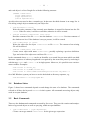
such a tuple type. For instance
rel(tuple([name: string, pop: int]))
is the type of a relation containing tuples consisting of two attribute values, namely name of type
string and pop of type int. A valid value of this type in nested list representation is a list containing lists of attributes of values, e.g.
(
(“New York” 732200)
(“Paris” 2175000)
(“Hagen” 212000)
)
6.3.2
Relation Operators
Table 8 shows a selection of the operators provided by the relational algebra module. Some of the
operators are overloaded. For more information about the operators and a full list of operators
type list algebra RelationAlgebra in the SECONDO user interface.
Here in the description of signatures, type constructors are denoted in lower case whereas words
starting with a capital denote type variables. Note that type variables occurring several times in a
signature must be instantiated with the same type.
Operator
Signature
Syntax
Semantics
feed
rel(Tuple) -> stream(Tuple)
_ #
Produces a stream of tuples from
a relation.
consume
stream(Tuple) -> rel(Tuple)
_ #
Produces a relation from a stream
of tuples.
filter
stream(Tuple) x (Tuple -> bool)
-> stream(Tuple)
_ # [ _ ]
Lets pass those input tuples for
which the parameter function
evaluates to TRUE.
Table 8: Relation Operators
–
34
–
attr
tuple([a1:t1, ..., an:tn]) x ai
-> ti
# (_ , _)
retrieves an attribute value from
a tuple
project
stream(Tuple1) x attrname+
-> stream(Tuple2)
_ # [ _ ]
relational projection operator (on
streams); no duplicate removal
product
stream(Tup1) x stream(Tup2)
-> stream(Tup3)
_ _ #
relational Cartesian product
operator on streams
count
stream(Tuple) -> int
rel(Tuple) -> int
_ #
Counts the number of tuples in a
stream or a relation.
rename
stream(Tuple1) x id
-> stream(Tuple2)
_ { _ }
Changes only the type, not the
value of a stream by appending
the characters supplied in arg2 to
each attribute name. The first
character of arg2 must be a letter.
Used to avoid name conflicts,
e.g. in joins.
(special
syntax,
operator name
not
needed)
Table 8: Relation Operators
Examples for the use of the operators listed in Table 8 are given in Section 6.4.2.
6.4
Extended Relation Algebra
6.4.1
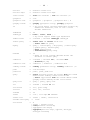
Extended Relation Operators
Beyond the operators provided by the relational algebra module a set of more sophisticated operators for relations is contained in the Extended Relation Algebra. This module adds no new types,
but operators for modification, extension, sorting and grouping of relations instead. The operator
table is structured similarly to the table above.
Operator
Signature
Syntax
Semantics
extract
stream(tuple([a1:t1, ...,
an:tn])) x ai
-> ti
_ # [ _ ]
Returns the value of a specified
attribute of the first tuple in the
input stream.
extend
stream(tuple([a1:t1, ...,
an:tn]) x
[(b1 x (Tuple -> u1)) ...
(bj x (Tuple -> uj))]
-> stream(tuple([a1:t1, ...,
an:tn, b1:u1, ..., bj:uj]))
_ # [ _ ]
Extends each input tuple by new
attributes. The second argument
is a list of pairs; each pair consists of a name for a new attribute
and an expression to compute the
value of that attribute. Result
tuples contain the original
attributes and the new attributes.
Refer to example 2 in Table 10.
Table 9: Extended Relation Operators
–
35
–
loopjoin
stream(Tuple1) x (Tuple1 ->
stream(Tuple2)))
-> stream(Tuple3)
_ # [ _ ]
Join operator performing a
nested loop join. Each tuple of
the outer stream is passed as an
argument to the second argument
function which computes an
inner stream of tuples. The operator returns the concatenation of
each tuple of the outer stream
with each tuple produced in the
inner stream.
mergejoin
stream(Tuple1) x stream(Tuple2)
x attr1 x attr2
-> stream(Tuple3)
_ _ #
[ _ , _ ]
Join operator performing merge
join on two streams w.r.t. attr1
of the first and attr2 of the second stream. The first argument
stream must be ordered by
attr1, the second by attr2, both
either ascending or descending.
sortmergejoin
stream(Tuple1) x stream(Tuple2)
x attr1 x attr2
-> stream(Tuple3)
_ _ #
[ _ , _ ]
Join operator performing merge
join on two streams w.r.t. attr1
of the first and attr2 of the second stream.
hashjoin
stream(Tuple1) x stream(Tuple2)
x attr1 x attr2 x int
-> stream(Tuple3)
_ _ # [ _
, _ , _ ]
Join operator performing hash
join on two streams w.r.t. attr1
of the first and attr2 of the second stream. The number of buckets used is specified by the fifth
argument.
symmjoin
stream(tuple(a1 ... an)) x
stream(tuple(b1 ... bm)) x
(tuple(a1 ... an) x
tuple(b1 ... bm) -> bool)
-> stream tuple(a1 ... an b1
... bm)
_ _ #
[ _ ]
Join operator performing symmetric join on two streams by
computing a Cartesian product
stream from its argument streams
and filtering by the third argument.
concat
stream(Tuple) x stream(Tuple)
-> stream(Tuple)
_ _ #
Concatenates two streams. Can
be used to implement relational
union (without duplicate
removal).
mergesec
stream(Tuple) x stream(Tuple)
-> stream(Tuple)
_ _ #
Intersection. Both streams must
be ordered (lexicographically by
all attributes, achieved by applying a sort operator before).
mergediff
stream(Tuple) x stream(Tuple)
-> stream(Tuple)
_ _ #
Difference on two ordered
streams.
Table 9: Extended Relation Operators
–
36
–
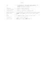
aggregate
stream(tuple((a1 t1) ... (an
tn))) x ai x (ti x ti -> ti) x
ti
-> ti
_ # [ _ ;
_ ; _ ]
Given an input stream, aggregates all values of a selected
attribute ai of all tuples of that
stream using the given aggregation function and an initial value.
See also aggregateB in the operator list in the system and the
example in Table 10.
groupby
stream(Tuple) x
[a1 ... ai] x
[(b1 x (rel(Tuple) -> u1))...
(bj x (rel(Tuple) -> uj))]
-> stream(tuple([a1:t1, ...,
ai:ti, b1:u1, ..., bj:uj]))
_ #
[ _ ; _ ]
Groups a stream by the attributes
given in the second argument.
The third argument is a list of
pairs; each pair consists of a
name for a new attribute and an
expression to compute the value
of that attribute from a subrelation obtained by grouping. Result
tuples contain the grouping
attributes and the new attributes.
See the example in Table 10. It is
possible to group by no attribute
(second argument remains
empty). In that case, the complete input stream forms a single
group.
sortby
stream(Tuple) x
(attr_i x dir_i)+
-> stream(Tuple)
_ # [ _ ]
Operator for sorting a stream lexicographically by one or more
attributes. For each attribute, the
“direction” of sorting can be
specified as either ascending
(asc) or descending (desc). If
neither (asc) nor (desc) is specified, that attribute is sorted in
ascending order.
sort
stream(Tuple) -> stream(Tuple)
_ #
Sorts the input tuple stream lexicographically ascending by all
attributes.
rdup
stream(Tuple) -> stream(Tuple)
_ #
Removes duplicates from a
totally ordered input stream.
min, max,
sum
stream(Tuple) x intattrname
-> int
stream(Tup) x realattrname
-> real
_ # [ _ ]
Returns the minimum, maximum, or sum value of the specified column. The second
argument must be the name of an
integer or real attribute.
avg
stream(Tuple) x numattrname
-> real
_ # [ _ ]
Returns the average value of the
specified column. The second
argument must be the name of an
integer or real attribute.
head
stream(Tuple) x int ->
stream(Tuple)
_ # [ _ ]
Returns the first n elements of
the input stream.
Table 9: Extended Relation Operators
–
6.4.2
37
–
Query Examples (Relation Algebra and Extended Relation Algebra)
To make it easier to understand how to use the operations of the relational algebra, a small database is available for this purpose. It is called testqueries and can be created and loaded as follows (from the secondo/bin directory):
create database testqueries;
restore database testqueries from testqueries;
Now the database is loaded. It provides (among others) the following simple relations:
tenTest:
twentyTest:
EmployeeTest:
DeptTest:
StaedteTest:
rel(tuple([no: int]))
rel(tuple([no: int]))
rel(tuple([EName: string, EmpNr: int, DeptNr: int]))
rel(tuple([Leader: string, DeptNr: int]))
rel(tuple([SName: string, Bev: int,
PLZ: int, Vorwahl: string, Kennzeichen: string]))
A first query example (in text syntax) is the following:
query tenTest feed filter [.no > 5] consume;
is the keyword to start a query. Next, tenTest selects the relation used in the query. feed
and consume are operators to produce a stream of tuples from a relation and produce a relation
from a stream of tuples, respectively. The filter operation has a parameter function [.no > 5]
and removes all tuples from the stream which evaluate to FALSE.
query
As we can see, the query in text syntax can be read from the beginning to the end: first, the relation is selected and a tuple stream is generated. For every single tuple the filter operation is
evaluated. After that, the remaining tuples are collected and a new relation is built.
As a second example we take
query tenTest feed twentyTest feed {A} product project[no_A] sort
rdup count;
Now we use two different relations (tenTest and twentyTest). Since the attribute names of both
relations are the same (they both have the attribute no), we have to use the rename operation,
which renames the attribute in the second relation by appending the attribute’s name with the passed character string. After that the product of both relations is computed. An attribute name (the
new name no_A) is passed to the project operator; after the projection to this attribute the tuples
of the stream are sorted and duplicates are removed. Finally the number of tuples is counted by
the count operation. The accurate result is 20.
Some more example queries are given in Table 10.
–
38
–
Text Syntax
Nested List Syntax
query StaedteTest feed
avg[Bev];
(query
(avg
(feed StaedteTest)
Bev));
query tenTest feed
extend[mod2: .no mod 2]
head[3]
consume;
(query
(consume
(head
(extend
(feed tenTest)
( (mod2
(fun (tuple1 TUPLE)
(mod
(attr tuple1 no)
2)))))
3)));
query StaedteTest feed
filter [.SName contains
"burg"]
project [SName,Kennzeichen]
consume;
(query
(consume
(project
(filter
(feed StaedteTest)
(fun
(tuple1 TUPLE)
(contains
(attr tuple1 SName)
"burg")))
(SName Kennzeichen))));
query EmployeeTest feed
sortby[DeptNr asc]
groupby[DeptNr;
anz: group feed count]
consume;
(query
(consume
(groupby
(sortby
(feed EmployeeTest)
( (DeptNr asc)))
(DeptNr)
( (anz
(fun (group1 GROUP)
(count
(feed group1))))))));
[Attention! Avoid semicolons followed
by a linebreak within queries! The
semicolon at the end of a line is interpreted as the end of the command!]
query StaedteTest feed
max[SName];
(query
(max
(feed StaedteTest)
SName));
query tenTest feed
aggregate[no; fun(i1: int,
i2: int) i1 * i2; 1]
(query
(aggregate
(feed tenTest)
no
(fun
(i1 int)
(i2 int)
(* i1 i2))
1))
Table 10: Query Examples (Relation Algebra)
–
39
–
7 Functions and Function Objects
A fundamental facility in SECONDO is the possibility to treat functions as values. We have already
seen anonymous parameter functions to operators such as select or filter. The type of a
function
fun (<arg_1>: <type_1>, ..., <arg_n>: <type_n>) <expr>
is
map(<type1>, ..., <type_n>, <resulttype>)
where <resulttype> is the type of <expr>. For example, the type of the function
fun (n: int) n + 1
is
map(int, int)
It is possible to create named SECONDO objects whose values are functions; technically the type
constructor map is provided by the FunctionAlgebra. Hence we can say:
create double: map(int,int)
update double := fun (n: int) n + n
It is easier to create a function object through the let command:
let prod = fun (n: int, m: int) m * n
We can ask for the value of a function object:
query prod
As a result, the type and the value of the function are displayed in nested list syntax:
Function type:
(map int int int)
Function value:
(fun
(n int)
(m int)
(* m n))
Function objects can be applied to arguments in the usual syntax and mixed with other operations:
query prod(5, double(7 * 6)) + 50
It is also possible to apply anonymous functions to arguments (this works only in nested list syntax):
(<anonymous function> <arg1> ... <arg_n>)
For example, we can write
(query ((fun (n int) (+ n 1)) 70))
and get as a result 71. It is allowed to define function objects with zero arguments; this can be
used to define views. For example, given a relation Staedte similar to StaedteTest from Section 6.3 we can define a view to get cities with more than 500000 inhabitants:
–
40
–
let Grossstaedte = fun () Staedte feed filter[.Bev > 500000] consume
Then the command
query Grossstaedte
yields the definition of the function:
Function type:
(map
(rel
(tuple
(
(SName string)
(Bev int)
(PLZ int)
(Vorwahl string)
(Kennzeichen string)))))
Function value:
(fun
(consume
(filter
(feed Staedte)
(fun
(tuple1 TUPLE)
(>
(attr tuple1 Bev)
500000)))))
Observe that the map constructor has only one argument, the result type. The function is applied
(evaluated) by writing
query Grossstaedte()
Such a view can be used in further processing, for example:
query Grossstaedte() feed project[SName] consume
and it can even be used in further views:
let Grosse = fun () Grossstaedte() feed project[SName] consume
As a final example, let us define a function that for a given string argument returns the number of
cities starting with that string:
let Staedte_with = fun (s: string) Staedte feed filter[.SName starts s]
count
Then
query Staedte_with(“B”)
returns on our little example relation the value 7.
–
41
–
8 The Optimizer
The optimizer component of SECONDO is written in PROLOG and allows one to formulate SECONDO commands as well as queries in an SQL-like language within a PROLOG environment.
Commands are passed directly to the SECONDO kernel for execution. Queries are translated to
query plans which are then also sent to the kernel for exection. One can also experiment with the
optimizer and just see how queries are translated without executing them.
In the following sections after some preparations we discuss the PROLOG environment, the
query language, hybrid queries (combining SQL with SECONDO operations) and creation of
objects from query results, the optimizer’s knowledge about databases, and how the optimizer can
be informed about new operators available in SECONDO.
8.1
Preparations
In the following examples, we work with the database opt. Hence, enter at any of the user interfaces (e.g. in SecondoTTYBDB) the commands:
create database opt
restore database opt from opt
Now the database is in good shape. When you type list objects, you can see that it has the following relations:1
Orte(Kennzeichen: string, Ort: string, Vorwahl: string, BevT: int)
Staedte(SName: string, Bev: int, PLZ: int Vorwahl: string,
Kennzeichen: string)
plz(PLZ: int, Ort: string)
ten(no: int)
thousand(no: int)
Furthermore, there are the two indexes plz_Ort_btree and plz_PLZ_btree which index on the
plz relation the attributes Ort and PLZ, respectively. All relations are small except for plz which
is a bit larger, having 41267 tuples.
8.2
Using SECONDO in a PROLOG environment
In Section 5 it was already discussed how the optimizer can be called. In this section, we assume
that the single user version SecondoPL is used; the client-server interface SecondoPLCS behaves
similarly. Hence, switch to the directory Optimizer and call the optimizer by the command:
SecondoPL
After some messages, there appears a PROLOG prompt:
1 ?-
1. There is also a further relation SEC_DERIVED_OBJ used internally to restore indexes and other derived
objects, and some more system tables starting SEC2... System tables can be queried like any relation, but they
are not persistent and will get lost between two sessions.
–
42
–
When the optimizer is used for the first time after installing SECONDO, some error messages
appear; these can safely be ignored. The reason is that some files generated by the running optimizer are not yet there.
We now have a PROLOG interpreter running which understands an additional predicate:
secondo(Command, Result) :- execute the Secondo command Command and get
the result in Result.
So at the command line, one can type:
1 ?- secondo('open database opt', Res).
This is executed, some SECONDO messages appear, and then the PROLOG interpreter shows the
result of binding variable Res:
Res = []
This is the empty list that SECONDO returns on executing successfully such a command, converted
to a PROLOG list. As usual with a PROLOG interpreter we can type <return> to accept the first
solution, or ;<return> to see more solutions (if any exist). After typing <return>, the interpreter responds
Yes
2 ?-
Let us try another command:
2 ?- secondo('query Staedte feed filter[.Bev > 500000] head[3]
|
consume', R), R = [First, _].
Here at the end of the first line we typed <return>, the interpreter then put “|
“ at the beginning of the next line. The PROLOG goal is complete only with the final “.” symbol, only then
interpretation is started. Here as a result we get after some SECONDO messages the result of the
query shown in variable R and the first element in variable First. This illustrates that, of course,
we can process SECONDO results further in the PROLOG environment.
By the way, when you later want to quit the running SecondoPL program, just type at the prompt
either
.. ?- halt.
or
.. ?- quit.
The first is the standard PROLOG termination, the second has been introduced to be consistent
with other SECONDO interfaces. In the sequel, we omit the PROLOG prompt in the examples.
There is also a version of the secondo predicate that has only one argument:
secondo(Command) :- execute the Secondo command Command and pretty-print
the result, if any.
Hence we can say:
secondo(’query Staedte’).
The result is printed in a similar format as in SecondoTTYBDB or SecondoTTYCS.
–
43
–
In addition, a number of predicates are available that mimic some frequently used SECONDO commands, namely
open
create
update
let
delete
query
They all take a character string as a single argument, containing the rest of the command, and are
defined in PROLOG to be prefix operators, hence we can write:
secondo(’close database’).
open ’database opt’.
create ’x: int’.
update ’x := Staedte feed count’.
let ’double = fun(n: int) 2 * n’.
query ’double(x)’.
delete ’x’.
In the remainder of this chapter, we assume that the “standard” version of the optimizer is active.
To ensure this, type
setOption(standard).
after starting SecondoPL. This command will do some output. If you type
showOptions.
an overview of all available options is printed. A marked checkbox in front of option “standard”
indicates, that it is active. By now, only option ’standard’ should be marked.
8.3
An SQL-like Query Language
The optimizer implements a part of an SQL-like language by a predicate sql, to be written in prefix notation, and provides some operator definitions and priorities, e.g. for select, from, where,
that allow us to write an SQL query directly as a PROLOG term. For example, one can write
(assuming database opt is open):
sql select * from staedte where bev > 500000.
Note that in this environment all relation names and attribute names are written in lower case letters only. Remember that words starting with a capital are variables in PROLOG; therefore we
cannot use such words. The optimizer on its own gets information from the SECONDO kernel
about the spellings of relation and attribute names and sends query plans to SECONDO with the
correct spelling.
Some messages appear that tell you something about the inner workings of the optimizer. Possibly the optimizer sends by itself some small queries to SECONDO, then it says:
Destination node 1 reached at iteration 1
Height of search tree for boundary is 0
The best plan is:
–
44
–
Staedte feed filter[.Bev > 500000] {0.20669, 3.27586} consume
Estimated Cost: 310.64
After that appear evaluation messages and the result of the query. If you are interested in understanding how the optimizer works, please read the paper [GBA+04]. If you wish to understand the
working of the optimizer in more detail, you can also read the source code documentation, that is,
say in the directory Optimizer:
pdview optimizer.pl
Almost all prolog sourcefiles (having filename extension .pl) from the Optimizer directory can
be processed in this way. In the following, we describe the currently implemented query language
in detail. Whereas the syntax resembles SQL, no attempt is made to be consistent with any particular SQL standard.
Basic Queries
The SQL kernel implemented by the optimizer basically has the following syntax:
select <attr-list>
from <rel-list>
where <pred-list>
Each of the lists has to be written in PROLOG syntax (i.e., in square brackets, entries separated by
comma). If any of the lists has only a single element, the square brackets can be omitted. Instead
of an attribute list one can also write “*”. Hence one can write (don’t forget to type sql before all
such queries and end them with a “.”):
select [sname, bev]
from staedte
where [bev > 270000, sname starts “S”]
To avoid name conflicts, one can introduce explicit variables. In this case one refers to attributes
in the form <variable>:<attr>. For example, one can perform a join between relations Orte
and plz:
select * from [orte as o, plz as p]
where [o:ort = p:ort, o:ort contains "dorf", (p:plz mod 13) = 0]
In the sequel, we define the syntax precisely by giving a grammar. For the basic queries described
so far we have the following grammar rules:
query
->
distinct-clause ->
select distinct-clause sel-clause
from rel-clause
where-clause
all | distinct |
ε
sel-clause
->
*
| result | [result-list]
| count(distinct-clause *)
result
->
attr | attr-expr as newname
result-list
->
result | result, result-list
–
45
–
attr
->
attrname | var:attrname
attr-list
->
attr | attr, attr-list
attrname
->
id
rel
->
relname | relname as var
rel-clause
->
rel | [rel-list]
rel-list
->
rel | rel, rel-list
relname
->
id
var
->
id
where-clause
->
where [pred-list] | where pred |
pred
->
attr-boolexpr
pred-list
->
pred | pred, pred-list
ε
We use the following notational conventions. Words written in normal font are grammar symbols
(non-terminals), words in bold face are terminal symbols. The symbols “->” and “|” are metasymbols denoting derivation in the grammar and separation of alternatives. “ε” denotes the empty
word. Other characters like “*” or “:” are also terminals. „id“ is any valid SECONDO identifier
(spelled in lower case letters).
The notation X-list refers to a non-empty PROLOG list with elements of type X; as mentioned
already, the square brackets can be omitted if the list has just one element.
The notation X-expr refers to an expression built from elements of type X, constants, and operations available on X-values. Hence attr-expr is an expression involving attributes denoted in
one of the two forms attrname or var:attrname. Similarly a predicate (pred) is a boolean
expression over attributes (attr-boolexpr).
X-constant
denotes a SECONDO constant of type X.
Finally, “ε” denotes the empty alternative. Hence the where-clause or the distinct keyword are
optional.
From the grammar, one can see that it is also possible to compute derived attributes in the selectclause. For example:
select [sname, bev div 1000 as bevt] from staedte
Order
One can add an orderby-clause (and a first-clause, see below), hence the syntax of a query is more
completely:
query
->
orderby-clause
orderby-clause
orderattr
orderattr-list
->
->
->
->
select distinct-clause sel-clause
from rel-clause
where-clause orderby-clause first-clause
orderby [orderattr-list] | orderby orderattr |
orderby [orderattr-list] | orderby orderattr |
attrname | attrname asc | attrname desc
orderattr | orderattr, orderattr-list
ε
ε
–
46
–
For example, we can say:
select [o:ort, p1:plz, p2:plz]
from [orte as o, plz as p1, plz as p2]
where [o:ort = p1:ort, p2:plz = (p1:plz + 1), o:ort contains "dorf"]
orderby [o:ort asc, p2:plz desc]
It is possible to mention derived attributes in the orderby-clause.
Taking Only the First n Elements
Sometimes one is interested in only the first few tuples of a query result. This can be achieved by
using a first-clause:
first-clause
->
first int-constant |
ε
For example:
select * from plz orderby ort desc first 3
This is also a convenient way to see the beginning of a large relation. Only the first few tuples are
processed.
Grouping and Aggregation
Aggregation queries have a groupby-clause in addition to what is known already and a different
form of the select-clause.
query
->
select aggr-clause from rel-clause
where-clause
groupby-clause
orderby-clause first-clause
aggr-clause
->
aggr2 | [aggr2, aggr-list]
aggr2
->
aggr
->
groupattr | groupattr as newname | aggr2
aggr-list
->
aggr | aggr, aggr-list
aggrop
->
min | max | sum | avg | extract | count
aggr-fun
->
(*) | (+) | union_new | intersection_new |
% any name fun of a binary SECONDO-operator or
function object with syntax fun: T x T -> T
which should be associative and commutative. Infixoperators must be inclosed in round paranthesis.
arbitrary-aggr
->
aggregate(ext-attr-expr, aggrfun, datatype,
datatype-constant)
datatype
count(distinct-clause *) as newname
| aggrop(ext-attr-expr) as newname
| arbitrary-aggr as newname
->
int | real | bool | string | line | points
| mpoint | uregion |
% any name of a SECONDO-datatype
groupattr
->
attr
groupattr-list
->
groupattr | groupattr, groupattr-list
–
groupby-clause
->
47
–
groupby [groupattr-list] | groupby groupattr
For example, one can say:
select [ort, min(plz) as minplz, max(plz) as maxplz, count(*) as cntplz]
from plz
where plz > 40000
groupby ort
orderby cntplz desc
first 10
Entries in the select-clause are either attributes used in the grouping or definitions of derived
attributes which are obtained by evaluating aggregate functions on the group. Again one can order
by such derived values. An aggregate operator like sum cannot only be applied to an attribute
name, but also to an expression built over attributes.
There is one restriction imposed by the current implementation and not visible in the grammar:
the select-clause in an aggregate query must contain a derived attribute definition. Hence
select ort from plz groupby ort
will not work. This will be optimized but not executed by SECONDO.
Union and Intersection
It is possible to form the union or intersection of a set of relations each of which is the result of a
separate query. The queries are written in a PROLOG list. All result relations must have the same
schema.
mquery
query-list
->
query
| union [query-list]
| intersection [query-list]
-> query | query, query-list
For example:
union [
select * from plz where ort contains “dorf”,
select * from plz where ort contains “stadt”]
Note that in this case, each of the subqueries in the list is optimized separately. One interesting
application is to find tuples in a relation fulfilling a very large set of conditions. The optimizer’s
effort in optimizing a single query is exponential in the number of predicates. It works fine
roughly up to 10 predicates. Beyond that optimization times get long. However, it is no problem
to use, for example, an intersection query on 30 subqueries each of which has only one or a few
conditions.
The query processed by the optimizer is an mquery, i.e., the query command is of the form
sql mquery.
The complete grammar can be found in Appendix B.
–
8.4
48
–
Further Ways of Querying
The basic form of querying is using the sql predicate in prefix notation, as explained in the previous section, hence
sql Term.
Hybrid Queries
A second form of the sql predicate allows one to further process the result of a query by SECONDO operators:
sql(Term, SecondoQueryRest).
Here SecondoQueryRest contains a character string with SECONDO operators, applicable to a
stream of tuples returned by the optimized and evaluated Term. For example:
sql(select * from orte where bevt > 300, 'project [Ort] consume').
Note that in the second argument, attribute names have to be spelled correctly as in writing executable queries to the SECONDO kernel. In this example, the same effect could have been achieved
by a pure SQL query, but there are cases when this facility is useful.
Creating Objects
The let command of SECONDO allows one to create SECONDO objects as the result of an executable query. There is a let predicate in the optimizer that allows one to do the same for the result
of an optimized query. There are two forms, the second one corresponding to a hybrid query.
let(ObjectName, Term).
let(ObjectName, Term, SecondoQueryRest).
For example:
let(orte2, select ort from [orte, plz as p] where ort = p:ort orderby ort,
'rdup consume').
This query creates a relation orte2 with the names of places (“Orte”) that also occur in the postal
code relation plz. Here duplicate removal was done at the executable level. However, it can also
be done directly, by saying:
let(orte3, select distinct ort from [orte, plz as p] where ort = p:ort
orderby ort).
Just Optimizing
For experimenting with the optimizer it is useful to optimize queries without executing them. This
is provided by the optimize predicate.
optimize(Term).
This returns the query plan and the expected cost.
–
8.5
49
–
The Optimizer’s Knowledge of Databases
The optimizer and the SECONDO kernel are only loosely coupled. In particular, one can use the
kernel independently, create and delete databases and objects within databases out of control of
the optimizer.
The optimizer maintains knowledge about the existing database contents within a number of
“dynamic predicates” while the optimizer is running, and in files between sessions. It obtains such
knowledge from the SECONDO kernel by sending commands or queries to it, for example, list
objects. Currently there are the following such predicates and corresponding files:
•
•
•
•
•
•
•
•
•
storedRels - relations and their attributes
storedSpells - spellings of relation and attribute names
storedIndexes - for which attributes do and do not exist indexes
storedCards - cardinalities of relations
storedTupleSizes - average tuple sizes (in bytes) of relations
storedSels - selectivities of selection and join predicates
storedPETs - predicate evaluation times for selection and join predicates
storedAttrSizes - average sizes of attributes in bytes
storedOrderings - known orderings within stored relations
The optimizer distinguishes between different databases by saving the database name with all
facts of its knowledge base.
The general principle is that the optimizer retrieves information from SECONDO when it is needed
and then stores it for later use. For example, when a relation is mentioned for the first time in a
query, the optimizer sends “list objects” to the kernel to check whether the relation exists and
to get attribute names with their spelling. It also determines whether there are indexes available
and creates a small sample relation if there is none yet. It sends a query “<relname> count” to
get the cardinality and another “<relname> tuplesize” to get the average tuple size in byte. It
also gets average attribute sizes by queries of the form “<relname> attrsize[<attrname>]”.
When in a query a selection or join predicate occurs for which the selectivity is not yet known, the
optimizer sends a corresponding query on the small sample relation(s) to determine the selectivity
and predicate evaluation time (PET).
Note: The optimizer recognizes indexes by a name convention. The name of an index must have
the form
<RelName>_<KeyattrName>_<LogicalIndexTypeCode>
is the name of the base relation, the index is built for, and <KeyattrName> is
the name (itentifier) of the attribute, that is used to generate the keys stored within the index.
<LogicalIndexTypeCode> is an alphanumerical code used to describe the logical index type.
While the base type of any index (rtee, rtree3, btree, xtree, hash etc.) can be looked up in the system catalog, the meaning of the index is coded using this tag. E.g. an rtree index can be described
as a temporal index built on single units of moving objects, or on the objects’ complete movement
here. This informatioon is used within optimization rules and required to construct small sample
objects used to determine selectivities and other parameters used during optimization. If this tag is
where <RelName>
–
50
–
left out, the logical index type is assumed to match the standard index type for the key attribute.
Logical index types are registered in file database.pl using facts logicalIndexType/8. The
names <RelName> and <KeyattrName> must be spelled as in the SECONDO kernel. Hence a ordinary B-tree index on attribute Bev of relation Staedte must be called Staedte_Bev_btree to be
recognized by the optimizer. Such an index can be created by the command:
let ’staedte_Bev_btree = Staedte createbtree[Bev]’.
Inquiries on the Optimizer’s Knowledge Base
The optimizer provides several commands for inquiries on its knowledge base:
•
•
•
•
•
- lists all known relations and their attributes
showStoredAttrSizes - lists types and sizes for known attributes
showStoredOrders - list known orderings
showSels - lists the known selectivities
showPETs - lists all known PETs
showStoredRels
The command
• showDatabase
will show a summary of all relation-based information gathered for the open database, including
information on attribute types and sizes, cardinalities and average tuple sizes, known indexes and
orderings. Last, the command
• showDatabaseSchema
will list all relations available in the open database (not only the ones known to the optimizer from
past queries) together with their attributes and attribute types.
Reinitializing
One can reinitialize the optimizer’s knowledge of databases by deleting the files storedRels etc.
mentioned above from the directory Optimizer (when the optimizer is not running). In this case,
all information needed will be collected afresh on further queries.
If you somehow run into unexplainable problems with the optimizer, it is usually a good idea to
quit the optimizer, delete all these stored*.pl files and restart the optimizer.
Creating and Deleting Relations
When new relation objects are created, the optimizer should recognize them automatically as
soon as they are used in a query. It will also notice, if a relation is deleted by the optimizer (of
course), and between two optimizer sessions. However, the optimizer will not automatically be
aware that a relation has been deleted during a optimizer session by third party and will still create
query plans for it which will then be refused by the SECONDO kernel. We explain below how the
optimizer can be informed about the deletion.
–
51
–
Creating and Deleting Indexes
The optimizer checks for indexes when a relation is mentioned for the first time in a query.
Hence, it automatically recognizes indexes created together with a relation before querying. It
will also notice creation and deletion of indexes by the optimizer and between different optimizer
sessions. It will not notice changes inflicted by third party during an optimizer session (but can be
instructed to rebuild its information base).
Informing the Optimizer
If the optimizer opens a database, it will automatically update its catalog on relations and indexes.
Additionally, three commands (predicates) are available to explicitly inform the optimizer about
changes to relations and indexes.
updateRel(Rel)
A call of this predicate causes the optimizer to delete all information it has about the relation Rel,
including selectivities of predicates. An existing sample is also destroyed. A query afterwards
involving this relation collects all information from scratch. Existing or non-existing indexes are
also discovered. For example:
updateRel(plz).
resets all information for relation plz. The second predicate is:
updateCatalog.
This predicate lets the optimizer perform the same procedure as if the currently open database was
reopened. In particular, it will check whether any relations and/ or indexes have been added or
removed, and update its knowledge base accordingly. Hence this can be used after creating or
destroying an index by third party, without losing all the other information collected for relation
Rel. For example, after deleting the index plz_Ort_btree one should inform the optimizer by
saying updateCatalog once.
updateDB(DB).
To update the metadata on a distinct (and closed) database, this predicate can be called. It will
retract all metadata on objects within that database. When the database is opened for the next
time, the optimizer will need to recollect metadata.
Creating Sample Relations Manually
As mentioned above, the optimizer uses small sample relations to determine selectivities of selection or join predicates before actually optimizing the query. These sample relations are normally
created automatically, with default sizes. There is one sample relation called <relname>_sample_s and another one called <relname>_sample_j, to be used for selection and join
predicates, and with default sizes 2000 and 500 tuples, respectively. If a relation has less tuples
than that, the sample will be the full relation.
However, in some cases this default value is not appropriate. This is mainly the case when a relation has few tuples containing large objects. Assuming, there is a database germany providing a
–
52
–
relation County with 439 tuples, each containing a region value with several hundred or thousand
edges. In this case a sample with 10% of the tuples is quite sufficient and preferable, as on the
geometries often expensive predicates are evaluated. hence in such a case one would like to have
samples of size 50, say, for both selection and joins.
Unfortunately it is difficult to build a general rule for such samples into the optimizer, and this has
not been done. Instead, the optimizer complains if by default it would create a sample relation of
size more than 2 MB, and asks the user to manually create samples. This can be done as follows.
The predicates
createSamples(RelName, SizeSel, SizeJoin).
resizeSamples(RelName, SizeSel, SizeJoin).
create samples with the desired sizes. While the first one only creates samples if they are not yet
present, the second one will also replace existent samples with new ones. Note that here the relation name has to be given in lower case letters only. For example:
resizeSamples(kreis, 50, 50).
If you do not want to be bothered by manual creation of samples, there is an option helpful to you:
setOption(autoSamples).
This will automatically create all samples needed using some heuristics to determine sample
sizes. However, with a database containing relations with large attribute values (like moving
object or multi media data), you might prefer manual mode. You can deactivate automatic sample
creation by writing
delOption(autoSamples).
8.6
Operator Syntax
In queries given to the optimizer one uses atomic operators in predicates and expressions in the
select-clause like
<, >, <=, #, starts, contains, +, *, div, mod
In this section we explain how new operators of this kind can be made available in the optimizer.
For using operators in queries, there are two conditions:
1. We must be able to write the operator in PROLOG.
2. The optimizer must know how to translate the operator application to SECONDO syntax.
PROLOG Syntax
Any operator can be written in PROLOG in prefix syntax. For example:
length(X), theDate(2004, 5, 9)
These are just standard terms in PROLOG. If we want to write a (binary) operator in infix notation, either this operator is defined already in PROLOG. This is the case for standard operators
–
53
–
like +, *, <, etc. Otherwise one can explicitly define it in the file opsyntax.pl in directory
Optimizer. For example, in the file we find definitions:
:::::-
op(800,
op(800,
op(800,
op(800,
op(800,
xfx, inside).
xfx, intersects).
xfx, adjacent).
xfx, or).
fx, not).
Here inside, intersects, adjacent, and or are defined to be binary infix operators, and not is
defined to be a unary prefix operator. New operators can be made available in the same way.
SECONDO Syntax
Translation to SECONDO is controlled firstly, by a few defaults, depending on the number of arguments:
• one argument: translated to prefix notation
op(arg)
• two arguments: translated to infix notation
arg1 op arg2
• three arguments: translated to prefix notation
op(arg1, arg2, arg3)
If a binary operator is to be translated to prefix notation instead, one can place a fact into the file
opsyntax.pl of the form
secondoOp(Op, prefix, 2)
For example, to define a distance operator with two arguments to be written in prefix notation
we can specify:
secondoOp(distance, prefix, 2).
Reload the file after modifying it:
[opsyntax].
Examples from the current contents of the file are shown in Appendix A. For example, we can
now use the distance operator in a query (on a database germany):
select [sname, distance(ort, s2:ort) as dist]
from [stadt, stadt as s2]
where [s2:sname = "Dortmund", distance(ort, s2:ort) < 0.3]
SECONDO TypeMapping
Some of the optional optimizer extensions rely on exact information of the type of expressions
and subexpressions (e.g. single computed arguments within a predicate). To this end, the
typemapping functions from within the SECONDO kernel have an equivalent within the optimizer.
Also, it is possible to assign properties to operators. For each operator, at least one predicate is
defined in file operators.pl:
opSignature(+Operator, +Algebra, +ArgTypeList, -Resulttype, -Flags).
–
54
–
For more information on operator signatures and properties, please read the comments within the
file operators.pl itself.
8.7
Optimizer Options
The optimizer includes several extensions and optional features, that can be selected and deselected at runtime. This is realized using optimizer options. When the optimizer starts up, a list of
all option settings is displayed. This list can be redisplayed using the command
showOptions.
The option list looks like the following:
Optimizer options (and sub-options):
[x] standard:
Adopt options for standard optimization process.
[ ] useCounters:
Insert counters into the computed plan.
[ ] noIndex:
Disables the utilization of indexes
[ ] allOff:
Turn off really ALL options.
[ ] earlyproject:
Project before sort and groupby
[ ] improvedcosts:
Use improved cost functions.
[ ] determinePredSig: Send queries to investigate predicate argument types.
[ ] immediatePlan:
Immediately create a path rather than the POG.
( ) intOrders(on):
Consider interesting orders (on-variant).
( ) intOrders(path): Consider interesting orders (path-variant).
( ) intOrders(quick): Consider interesting orders (quick-variant).
( ) intOrders(test):
Consider interesting orders (test-variant).
[ ] autoSamples:
Automatically determine sample sizes.
[ ] rewriteInference: Add inferred predicates to where clause.
( ) rtreeIndexRules:
Infer predicates to exploit R-tree indices.
( ) rewriteNonempty:
Handle 'nonempty' in select statements.
[ ] rewriteCSE:
Extend with attributes for CSE values.
( ) rewriteCSEall:
Extend with attributes for _ALL_ CSEs.
( ) rewriteRemove:
Remove attributes as early as possible.
[ ] debug:
Execute debugging code. Also use 'toggleDebug.'.
[ ] autosave:
Autosave option settings on 'halt.'.
[ ] noprogress:
Do not send predicate data for progress estimation.
[ ] subqueries:
Process subqueries.
( ) subqueryUnnesting: Apply unnesting algorithms to subqueries
[ ] entropy:
Use entropy maximization together with an exploration query on a small sample database
Type 'loadOptions.' to load the saved option configuration.
Type 'saveOptions.' to save current option configuration to disk.
Type 'defaultOptions.' to restore the default options.
Type 'setOption(X).' to select option X.
Type 'delOption(X).' to unselect option X.
Type 'showOptions.' to view this option list.
Type 'helpMe.' to get an overview on user level predicates.
Yes
Some of these options have been mentioned before. To select/ activate an option, say
setOption(OptionName).
to deselect/ deactivate an option
delOption(OptionName).
where OptionName is a term listed by showOptions.
–
55
–
Several options will automatically deactivate incompatible options and/or activate other options,
it depends on. Some options are suboptions, that change the behaviour of their super-option.
There are four options with a special meaning: standard, debug, autosave, and allOff.
Option standard will configure the option settings to what we call the optimizer’s standard
behaviour.
Option debug will activate debugging code within the optimizer. This will produce lots of debug
messages and will slow down query processing.
When option autosave is selected, the option settings will be saved during optimizer sessions.
When the next session is started, the settings of the previous settings will be restored. It is also
possible to manually save the current option settings using saveOptions. and to restore them using
defaultOptions.
Option allOff means, that all options are unselected (other than standard, that may activate
some options).
8.8
Getting Help on the Optimizer
The optimizer also has a built-in help function. It can be accessed by typing
helpMe.
After typing this command, a list of all user-level predicates is presented (which has been abbreviated here):
Help is available on the following user level predicates:
Predicate
/Arity Meaning
--------------------------------------------------------allCards
/0 Compare estimated and actual cardinalities for the current POG.
cdb
/0 Close current database.
closeDB
/0 Close current database.
cmdHist2File
/1 Dump the command history to a file.
create []
/1 Prepend 'create ' and send to DBMS-kernel.
createIndex
/3 Create an index of a specified type over a given attribute for a relation.
createSamples
/3 Create (but do not replace) samples for a relation.
debugLevel
/1 Add a given level to the debug list.
defaultOptions
/0 Choose the default option setting.
delOption
/1 Unset a given option.
delete []
/1 Prepend 'delete ' and send to DBMS-kernel.
deleteHistory
/0 Delete the query history relation 'SqlHistory' from the current DB.
derive []
/1 Prepend 'derive ' and send to DBMS-kernel.
writePlanEdgesX
/0 List executable and internal sub plans for all POG edges.
writeSizes
/0 List estimated cardinalities and selectivities for the current POG.
Use 'helpMe(Pred).' or 'helpMe(Pred,Arity).' for help on a certain predicate
It is also possible to ask for help on a certain predicate, say createIndex:
helpMe(createIndex).
After typing this command you can read:
Help on predicate 'createIndex/3':
Create an index of a specified type
–
56
–
over a given attribute for a relation.
createIndex(
+DCRel:
The relation the index is for.,
+DCAttr:
The key attribute.,
?LogicalIndexType: The logical index type.
)
This says, that the predicate createIndex has arity three (requires 3 arguments). Calling this
predicate will create an index. The meaning of the three arguments is explained. A ’+’ in front of
an argument means, that the argument must be bound to a value. A ’-’ means that the parameter is
an output parameter. A variable used here will be bound during the evaluation of the predicate. A
’?’ means that this parameter may be bound (e.i. acts as an input parameter) or unbound (i.e. acts
as a output parameter).
For some predicates, there are versions with different arities, e.g. helpMe. We can get an inroductory overview on all variant:
34 ?- helpMe(helpMe).
There are several arities for predicate 'helpMe'
Help is available on the following arities:
Predicate
/Arity Meaning
--------------------------------------------------------helpMe
/0 List available user level predicates.
helpMe
/1 Show help on a given user level predicate.
helpMe
/2 Show help on a user level predicate with a given arity.
Use 'helpMe(Pred,Arity).' for help on a certain arity of that predicate.
Yes
To get information on the predicate with a given arity, you can type e.g.
36 ?- helpMe(helpMe,2).
Help on predicate 'helpMe/2': Show help on a user level predicate with a
given arity.
helpMe(
+PredicateName:
The predicate to get information about.,
+Arity:
Chooses amongh predicates with more than one arity.
)
Yes
By this way, it is possible to browse information on all important user-level predicates.
–
A
Operator Syntax
/* [File ~opsyntax.pl~]
1 Query Language Operator Syntax
*/
::::::::::::::::::::::::::::::::::::::::::::::::::::::::-
op(200,
op(800,
op(800,
op(800,
op(800,
op(800,
op(800,
op(800,
op(800,
op(800,
op(800,
op(800,
op(800,
op(800,
op(800,
op(800,
op(800,
op(800,
op(800,
op(800,
op(800,
op(800,
op(800,
op(800,
op(800,
op(800,
op(800,
op(800,
op(800,
op(800,
op(800,
op(800,
op(800,
op(800,
op(800,
op(800,
op(800,
op(800,
op(800,
op(800,
op(800,
op(800,
op(800,
op(800,
op(800,
op(800,
op(800,
op(800,
op(800,
op(800,
op(800,
op(800,
op(800,
op(800,
op(800,
op(800,
xfx,
xfx,
xfx,
xfx,
xfx,
xfx,
xfx,
xfx,
xfx,
xfx,
xfx,
xfx,
xfx,
xfx,
xfx,
xf ,
xf ,
xf ,
xf ,
xf ,
xf ,
xf ,
xf ,
xf ,
xf ,
xf ,
xfx,
xfx,
xfx,
xfx,
xfx,
xfx,
xfx,
xfx,
xfx,
xfx,
xfx,
xfx,
xfx,
fx,
xfx,
xfx,
xfx,
xfx,
xfx,
xfx,
xfx,
xfx,
xfx,
xfx,
xfx,
xfx,
xfx,
xfx,
xfx,
xfx,
:).
=>).
<=).
#).
div).
mod).
and).
starts).
contains).
==).
##).
<<).
>>).
<<==).
>>==).
++).
category).
isgrayscale).
isportrait).
height).
leapyear).
line2region).
picturedate).
rect2region).
relcount).
relcount2).
inside).
insideold).
intersects).
adjacent).
attached).
overlaps).
onborder).
ininterior).
touchpoints).
intersection).
commonborder).
commonborderscan).
or).
not).
before).
present).
passes).
atinstant).
atperiods).
at).
satisfies).
when).
sometimes).
never).
always).
eplus).
simpleequals).
intersects_new).
p_intersects).
equalway).
57
–
–
58
–
/* Executable Language Operator Syntax
----secondoOp(?Op, ?Syntax, ?NoArgs) :---~Op~ is a Secondo operator written in ~Syntax~, with ~NoArgs~ arguments.
Currently implemented:
Quick Reference:
---OperatorSyntax
|
Use: OperatorType, Arity ( '_' = don't care)
-----------------------+-----------------------------------------------# ( _ )
|
(no explicit specification)
# ( _, _ )
|
prefix, 2
# ( _, _, _, ...)
|
(no explicit specification)
_ #
|
postfix, 1
_ # _
|
(no explicit specification)
_ # [ _ ]
|
postfixbrackets, _
_ # [ _, _ ]
|
postfixbrackets, _
_ # [ _, _, ... ]
|
postfixbrackets, _
_ _ #
|
postfix, 2
_ _ # [ _ ]
|
postfixbrackets2, _
_ _ # [ _, _ ]
|
postfixbrackets2, _
_ _ # [ _, _, ... ]
|
postfixbrackets2, _
_ _ _ #
|
postfix, 3
_ _ _ # [ _ ]
|
postfixbrackets3, _
_ _ _ # [ _, _ ]
|
postfixbrackets3, _
_ _ _ # [ _, _, ... ] |
postfixbrackets3, _
---*/
:- dynamic(secondoOp/3).
secondoOp(
secondoOp(
secondoOp(
secondoOp(
secondoOp(
secondoOp(
secondoOp(
secondoOp(
secondoOp(
secondoOp(
secondoOp(
++,
addcounter,
addid,
addtupleid,
approximate,
attr,
attrsize,
avg,
bbox,
between,
box3d,
postfix, 1).
postfixbrackets1,
postfix, 1).
postfix, 1).
postfixbrackets1,
prefix, 2).
postfixbrackets1,
postfixbrackets1,
prefix, 1).
postfixbrackets1,
prefix, 2).
.....
secondoOp( writeFile,
prefix, 2).
/* End of file ~opsyntax.pl~ */
3).
3).
2).
2).
3).
–
B
59
–
Grammar of the Query Language
We use the following notational conventions. Words written in normal font are grammar symbols
(non-terminals), words in bold face are terminal symbols. The symbols “->” and “|” are metasymbols denoting derivation in the grammar and separation of alternatives. Other characters like
“*”, “,” or “:” are also terminals.
The notation X-list refers to a PROLOG list with elements of type X; as mentioned already, the
square brackets can be omitted if the list has just one element. The notation X-expr refers to an
expression built from elements of type X, constants, and operations available on X-values. Hence
attr-expr is an expression involving attributes denoted in one of the two forms attrname or
var:attrname. Similarly a predicate (pred) is a boolean expression over attributes. X-constant
denotes a SECONDO constant of type X. Finally, “ε” denotes the empty alternative. For example,
the where-clause is optional.
sql-clause
->
let objectname mquery.
| let(objectname, mquery, secondo-rest-query).
| sql mquery.
| sql(mquery, secondo-rest-query).
aggr
->
groupattr | groupattr as newname | aggr2
aggr2
->
count(distinct-clause *) as newname
| aggrop(ext-attr-expr) as newname
| aggregate(ext-attr-expr, aggrfun, datatype,
datatype-constant) as newname
aggrop
->
min | max | sum | avg | extract | count
aggr-clause
->
aggr | [aggr, aggr-list]
aggr-fun
->
(*) | (+) | union_new | intersection_new |
% any name fun of a binary SECONDO-operator or
function object with syntax fun: T x T --> T
which should be associative and commutative.
Infix-operators must be inclosed in round
paranthesis.
aggr-list
->
aggr | aggr, aggr-list
attr
->
attrname | var:attrname | rowid
attr-list
->
attr | attr, attr-list
attrname
->
id
column
->
newname : datatype
column-list
->
column | column , column-list
create-query
->
create table newname columns [column-list]
| create index on relname columns index-clause
datatype
->
int | real | bool | string | line | points
| mpoint | uregion | ...
% any name of a SECONDO-datatype
delete-query
->
delete from rel-clause where-clause
distinct-clause
->
all | distinct |
drop-query
->
drop table relname
| drop index indexname
| drop index on relname index-clause
ε
–
60
–
ext-attr
->
distinct-clause attr
ext-attr-expr
->
distinct-clause attr-expr
first-clause
->
first int-constant | last int-constant |
groupattr
->
attr
groupattr-list
->
groupattr | groupattr , groupattr-list |
groupby-clause
->
groupby [groupattr-list] | groupby groupattr
id
->
% any valid Prolog constant-identifier without any
underscore character, that is also a valid
Secondo identifier
indexname
->
id
indextype
->
btree | rtree | hash | ...
% any valid logical index type expression
index-clause
->
attrname | attrname indextype indextype
insert-query
->
insert into rel values value-list
| insert into rel query
mquery
->
query | create-query | drop-query | insert-query
| update-query | delete-query
| union [query-list]
| intersection [query-list]
newname
->
id
% where id is not already defined within the
database or current query
orderattr
->
attrname | attrname asc | attrname desc
| distance(id, id)
orderattr-list
->
orderattr | orderattr , orderattr-list
orderby-clause
->
orderby [orderattr-list] | orderby orderattr |
pred
->
attr-boolexpr
pred-list
->
pred | pred, pred-list
query
->
select distinct-clause sel-clause from rel-clause
where-clause orderby-clause first-clause
| select aggr-clause from rel-clause where-clause
groupby-clause orderby-clause first-clause
query-list
->
query | query, query-list
rel
->
relname | relname as var
rel-clause
->
rel | [rel-list]
rel-list
->
rel | rel, rel-list
relname
->
id
result
->
attr | attr-expr as newname
result-list
->
result | result, result-list
secondo-rest-query
sel-clause
->
->
|
|
|
|
ε
ε
'text'
*
result | [result-list]
count(distinct-clause *)
aggrop(ext-attr-expr)
aggregate(ext-attr-expr, aggrfun, datatype,
datatype-constant)
ε
–
61
–
text
->
% any sequence of characters, that completes the
optimized query to a valid expression in
SECONDO executable language
transform
->
attrname = update-expression
transform-clause
->
transform | [transform-list]
transform-list
->
transform | transform, transform-list
update-expression ->
% a fixed value, or an operation calculating a value
update-query
->
update relname set transform-clause where-clause
var
->
id
value
->
% a PROLOG integer, boolen or string value
value-list
->
value | value, value-list
where-clause
->
where [pred-list] | where pred |
ε
–
C
62
–
References
[DG00]
Dieker, S., and R.H. Güting, Plug and Play with Query Algebras: SECONDO. A
Generic DBMS Development Environment. Proc. Int. Database Engineering and
Applications Symposium (IDEAS, Yokohama, Japan), 2000, 380-392.
[GBA+04] Güting, R.H., T. Behr, V.T. de Almeida, Z. Ding, F. Hoffmann, and M. Spiekermann,
SECONDO: An Extensible DBMS Architecture and Prototype. Fernuniversität
Hagen, Informatik-Report 313, 2004.
[Gü93]
Güting, R.H., Second-Order Signature: A Tool for Specifying Data Models, Query
Processing, and Optimization. In: Proc. ACM SIGMOD Conference. Washington,
USA, 1993, 277-286.