Download VocalTractLab 2.1 User Manual

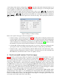
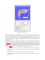
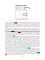
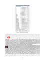
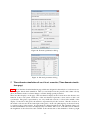
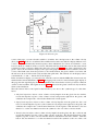
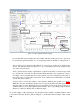
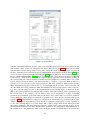
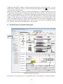
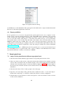
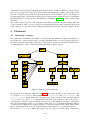
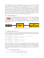
VocalTractLab 2.1 User Manual
Peter Birkholz
September 24, 2013
Contents
1
Introduction
1.1 Purpose . . . . . . . . . . . . . . . . . . . . . . . . . . . . . . . . . . . . . . . . . . .
1.2 Requirements, Known issues . . . . . . . . . . . . . . . . . . . . . . . . . . . . . . . .
1.3 Download, Installation, Registration . . . . . . . . . . . . . . . . . . . . . . . . . . . .
2
2
2
2
2
Overview
2.1 Computational models . . . . . . . . . . . . . . . . . . . . . . . . . . . . . . . . . . .
2.2 Graphical user interface (GUI) . . . . . . . . . . . . . . . . . . . . . . . . . . . . . . .
3
3
4
3
Basic signal analysis (Signal page)
5
4
Vocal tract model analysis (Vocal tract page)
6
5
Time-domain simulation of vocal tract acoustics (Time-domain simulation page)
6
Gestural score (Gestural score page)
6.1 The concept of gestural scores .
6.2 Editing a gestural score . . . . .
6.3 Copy synthesis . . . . . . . . .
6.4 Export possibilities . . . . . . .
13
.
.
.
.
.
.
.
.
.
.
.
.
.
.
.
.
.
.
.
.
.
.
.
.
.
.
.
.
.
.
.
.
17
18
18
19
20
Some typical uses
7.1 Analysis of the glottal flow for different supraglottal loads . . . . . . . . .
7.2 Comparison of an utterance created by copy-synthesis with its master signal
7.3 Create and save a new vocal tract shape . . . . . . . . . . . . . . . . . . .
7.4 Fitting the vocal tract shape to contours in an image . . . . . . . . . . . . .
.
.
.
.
.
.
.
.
.
.
.
.
.
.
.
.
.
.
.
.
.
.
.
.
.
.
.
.
20
20
21
21
22
Miscellaneous
8.1 Tube synthesis . . . . . . . . . . . . . . . . . . . . . . . . . . . . . . . . . . . . . . . .
22
22
A File formats
A.1 Speaker file (*.speaker) . . . . . . . . . . . . . . . . . . . . . . . . . . . . . . . . . . .
A.2 Gestural score file (*.ges) . . . . . . . . . . . . . . . . . . . . . . . . . . . . . . . . . .
A.3 Segment sequence file (*.seg) . . . . . . . . . . . . . . . . . . . . . . . . . . . . . . . .
23
23
24
24
B Changes since VTL 2.0
25
References
26
7
8
.
.
.
.
.
.
.
.
.
.
.
.
.
.
.
.
.
.
.
.
1
.
.
.
.
.
.
.
.
.
.
.
.
.
.
.
.
.
.
.
.
.
.
.
.
.
.
.
.
.
.
.
.
.
.
.
.
.
.
.
.
.
.
.
.
.
.
.
.
.
.
.
.
.
.
.
.
.
.
.
.
.
.
.
.
.
.
.
.
1
1.1
Introduction
Purpose
VocalTractLab (VTL) is an articulatory speech synthesizer and a tool to visualize and explore the mechanism of speech production with regard to articulation, acoustics, and control. It is developed by Dr. Peter
Birkholz along with his research on articulatory speech synthesis. With VTL, you can, for example,
• analyze the relationship between articulation and acoustics of the vocal tract;
• synthesize vowels and consonants from arbitrary vocal tract shapes with different models for glottal excitation;
• synthesize vowels from an arbitrary set of formants and anti-formants;
• synthesize connected speech utterances based on gestural scores;
• analyze the time-varying distribution of pressure and volume velocity within the vocal tract during
the synthesis of speech.
However, VTL is not a text-to-speech system. At the moment, connected utterances can only be synthesized based on gestural scores, as described in Sec. 6.
1.2
Requirements, Known issues
VTL is currently developed for the Windows platform. It was tested with Windows 7 and Windows
XP, but should also run under Windows Vista and 8. The minimum screen resolution is 1024x768, but
higher resolutions are preferable. As the simulations are computationally intensive, a fast computer is
recommended. For these reasons, tablet computers and netbooks are generally not suited to work with
VTL.
There was no extensive testing of the software, but the parts of the program made available are considered
to be relatively stable. Please feel free to report any bugs to [email protected].
Currently, there is the following issue: With Windows Vista and 7, you should use the “Aero design” for
the desktop (this is the default). Otherwise, the model of the vocal tract, which is drawn using OpenGL,
might not be displayed properly.
To run VTL on other platforms than Windows, e.g., Linux or Mac, we recommend to use a virtual
machine, for example VirtualBox (www.virtualbox.org). Note that VTL comes with no warranty of
any kind. The whole software is under continual development and may undergo substantial changes in
future versions.
1.3
Download, Installation, Registration
The program is free of charge and available for download as a ZIP file from www.vocaltractlab.de. It
needs no special installation. Simply unzip the downloaded file into a folder of your choice and start the
program by calling “VocalTractLab2.exe”. The ZIP archive contains a couple of other data files, most
of which are example files. The only essential file next to the executable is “JD2.speaker”, which is an
XML file that defines the default speaker (see Sec. A.1) and is loaded automatically when VTL is started.
After downloading the program, it has a limited functionality. To get access to all functions, please
register your copy of VTL. Just write a short email containing your name, city, and institution to peter.
[email protected] with the request to register (free of charge). In response, you will receive
a personalized registration file activating all the functions described in this manual. Note that the response
may take a few days, as it is done manually. If you have a registration file for a previous version of the
software, you can also use it for the new version and don’t need to register again. Just copy the file
“registration.txt” into the folder with the new version.
2
2
2.1
Overview
Computational models
VTL implements various models, for example models for the vocal tract, the vocal folds, the acoustic
simulation etc. This section provides references to the most important models, which are a recommended
read if you wish to understand them in-depth.
The core of the synthesizer is a 3D articulatory model of the vocal tract that defines the shape of the airway between the glottis and the lips. It has currently 23 degrees of freedom (vocal tract parameters) that
control the shape and position of the model articulators. The model was originally developed by Birkholz
(2005) and later refined by Birkholz, Jackèl, and Kröger (2006), and Birkholz and Kröger (2006). The
most recent version of the model is described by Birkholz (2013). For the simulation of acoustics, the
area function of the vocal tract is calculated, i.e., the variation of the cross-sectional area along the center
line of the model. The area function is then transformed into a transmission line model of the vocal tract
and can be analyzed in the frequency domain or simulated in the time domain. The basic method for the
analysis/synthesis is described by Birkholz and Jackèl (2004) and Birkholz (2005).
For the synthesis of vowels, there are two approaches in VTL: One convolves the glottal flow waveform
of the Liljencrants-Fant model for the glottal flow (Fant, Liljencrants, and Lin 1985) with the impulse
response of the vocal tract transfer function calculated in the frequency domain (similar to the method
by Sondhi and Schroeter 1987). The other one simulates the acoustic wave motion entirely in the time
domain based on a finite-difference scheme in combination with a model of the vocal folds attached
to the transmission-line model of the vocal tract. Currently, four vocal fold models are implemented:
the geometric model by Titze (1989), the classic two-mass model by Ishizaka and Flanagan (1972), a
modified two-mass model by Birkholz, Kröger, and Neuschaefer-Rube (2011c) and Birkholz, Kröger,
and Neuschaefer-Rube (2011a), and a test version of an asymmetrical vocal fold model (unpublished).
These models can be individually parameterized and exchanged for the acoustic simulation, as described
by Birkholz and Neuschaefer-Rube (2012). Connected utterances based on gestural scores are always
simulated in the time domain, because this method can better account for dynamic and transient acoustic
effects. For the simulation of glottal and supraglottal noise sources, a noise source model based on the
aerodynamic-acoustic relations by Stevens (1998) is used. To better account for differences in noise
source properties depending on the constriction position, the concept of the “enhanced area function” to
represent the vocal tract shape was recently implemented in VTL (Birkholz submitted).
Coarticulatory effects of the vocal tract are modeled using a coarticulation model based on bilinear
interpolation, as described in (Birkholz 2013). In short, for each consonant, three vocal tract target
shapes were defined (in VTL, they were extracted from dynamic MRI data): one in the context of each
corner vowel /a, i, u/. For example, for the consonant /d/, we can denote these three shapes by /d(a)/,
/d(i)/, and /d(u)/. When /d/ has to be realized in the context of an arbitrary vowel V in the simulation,
the coarticulation model maps V into the parameter subspace of the vocal tract shapes for /a, i, u/. The
position in the subspace is then used to infer the “coarticulated” target shape of /d/ in the context of V
by bilinear interpolation between /d(a)/, /d(i)/, and /d(u)/. For example, when the vowel /E/ is halfway between /a/ and /i/, then the target shape for /d/ in the utterance /EdE/ is assumed to be half-way
between /d(a)/ and /d(i)/.
Connected utterances in VTL are defined by gestural scores, a concept taken from articulatory phonology
(Browman and Goldstein 1992). A gestural score consists of a number of independent tiers populated
with discrete gestures. Each gesture represents the movement of certain articulators (i.e., vocal tract
parameters) toward a target configuration. The change of vocal tract parameters in response to these discrete gestures is governed by linear dynamical systems. Details of the definition of gestural scores and the
mapping to articulatory trajectories is the subject of ongoing research. The basic principles underlying
the current implementation are discussed in Birkholz (2007) and Birkholz, Kröger, and NeuschaeferRube (2011b). In VTL 2.1, 5th order critically-damped linear systems are used to model the dynamics
of articulators.
3
2.2
Graphical user interface (GUI)
Record / Play / Play selection / Clear
Page
tabs
Detailed oscillogram
Zoomed section
Control panel
Overview oscillogram
Time mark
Spectrogram
Short-time Fourier transform
Figure 1: Signal page.
Fig. 1 shows the layout of the graphical user interface of VTL. From top to bottom, it consists of a title
bar, a menu bar, a toolbar, and the main window region. The title bar shows for whom the copy of the
program is registered. The menu bar has the six menus “File”, “Edit”, “Export”, “Synthesis models”,
“Tube synthesis” and “Help”. The items of these menus will be referred to in the subsequent sections.
The toolbar has four tools to record a sound from a microphone, to play the main audio track, to play a
selected part of the main audio track, and to clear certain user data, which can be selected from a pull
down menu.
The main window region shows one of four pages that can be selected with the page tabs below the
toolbar. Each page is dedicated to a certain aspect of the program.
• The signal page, which is shown in Fig. 1, is meant for the acoustic analysis of speech signals.
• The vocal tract page is meant for the analysis of the vocal tract model and the synthesis of vowels
in the frequency domain.
• The time-domain simulation page is meant for the analysis of vocal tract acoustics in the time
domain.
• The gestural score page is meant for the manual creation of gestural scores and the copy-synthesis
of natural utterances.
The following four sections explain the basic functionality of the pages. In general, each of the pages
consists of a main region that contains different displays, and a control panel at the left side. In addition
to the main window, many functions of VTL are controlled with individual dialogs that can be displayed
or hidden on demand. All the dialogs associated with the implemented synthesis models can be called
4
from the menu “Synthesis models”. The following abbreviations will be subsequently used: LMB = left
mouse button; RMB = right mouse button.
3
Basic signal analysis (Signal page)
The signal page provides displays and functions for the basic analysis of audio signals. VTL has three
tracks to store sampled signals. They are called “Main track”, “EGG track”, and “Extra track”. In most
cases, all audio analysis and synthesis takes place on the main track. The EGG track is meant to store
the Electroglottogram (EGG) signal corresponding to a speech signal in the main track. Finally, the extra
track can store a third signal for different purposes. For the copy-synthesis of speech based on gestural
scores (see Sec. 6), the extra track must contain the original (master) speech signal. Each track represents
a buffer of 60 s length with a sampling rate of 22050 Hz and a quantization of 16 bit. The menu “File”
has five items to load and save sampled signals:
• “Load WAV+EGG (stereo)” loads a stereo WAV file. The left channel is stored in the main track
and the right channel is assumed to represent the corresponding EGG signal and is stored in the
EGG track.
• “Save WAV+EGG (stereo)” saves the signal in the main track and the EGG track in the selected
time range (see below) to a stereo WAV file.
• “Load WAV” loads a mono WAV file to a track of your choice.
• “Save WAV” saves the signal in the selected time range from a track of your choice to a mono
WAV file.
• “Save WAV as TXT” saves the signal in the selected time range from a track of your choice as
numbers in a text file. This allows the samples of a signal to be easily imported into programs like
Matlab or MS Excel.
If the sampling rate of a WAV file to be loaded does not correspond to 22050 Hz, the sampling rate is
converted automatically.
There are four displays in the main part of the signal page (cf. Fig. 1): the detailed oscillogram, the
overview oscillogram, the spectrogram, and the short-time Fourier transform. With the checkboxes next
to the oscillogram display you can select the track(s) to display. For each track, the time signal is
displayed in a different color. The detailed oscillogram shows a detailed view of the highlighted part
in the middle of the overview oscillogram. For the track selected next to the spectrogram display, the
spectrogram is shown. Both the overview oscillogram and the spectrogram have the same time scale. You
can change the scale with the buttons “-” and “+” below the checkboxes next to the detailed oscillogram.
With the buttons “+” and “-” that are arranged vertically, you can adjust the amplitude scaling of the
signals for display. With the buttons “+” and “-” next to the word “Main” you can actually increase
or decrease the signal amplitude in the main track. However, when a signal has small amplitudes, it is
usually better to select the menu item “Edit → Normalize amplitude” or press the shortcut Ctrl + N to
increase the amplitude.
The buttons “Main <-> EGG” and “Main <-> Extra” swap the signals in the corresponding tracks. Use
the scrollbar between the oscillogram and the spectrogram to scroll through the tracks. Alternatively, use
Ctrl + ← or Ctrl + → . To select a time range of the signals, right-click in one of the oscillogram
displays and select to set the beginning or the end of the range in the context menu. The time range
selection is used to define the signal parts to be saved as WAV files or to be played with the “Play
selection” button in the toolbar. You can also clear the selected part of the signal with the menu item
“Edit → Set audio selection to zero".
When you left-click in the spectrogram or oscillogram displays, you move a time mark (cursor) to the
corresponding time in the signal. The short-time Fourier transform (or a different transform, depending
5
on the settings in the Analysis settings dialog in Fig. 2) at the time of the mark is displayed in the bottom
part on the page. To change the relative height of the four displays on the page, you can drag the splitter
controls right above and below the spectrogram window.
To record a microphone signal, press the red button in the toolbar or press Ctrl + R . The signal will
always be recorded to the main track. To play back the signal in the main track, press the green arrow in
the tollbar or press Ctrl + P . The green arrow between the two vertical lines or the key combination
Ctrl +
plays the main track signal in the selected time range. This signal part is played in a
loop.
Figure 2: Dialog for analysis settings.
In the control panel of the page are the following buttons:
• “Analysis settings” opens the dialog shown in Fig. 2. This dialog allows setting the parameters used
for the calculation of the spectrum in the bottom display, for the spectrogram, and the fundamental
frequency (F0) contour. Furthermore, a measure for voice quality (along the lax-tense continuum)
can be calculated based on the Peak Slope Parameter by Kane and Gobl (2011). Please note that
the calculation of glottal closure instants and formants is not yet implemented.
• “Calculate F0” calculates the F0 contour in the track of your choice, which can be displayed in the
spectrogram (set the corresponding check mark in the analysis settings dialog on the F0 tab).
• “Analysis results” opens a non-modal dialog where the F0 at the time of the mark in the oscillogram/spectrogram is displayed in semitones (relative to the musical note C0 with 16.352 Hz) and
Hz. Furthermore, the measured value for the voice quality is shown.
4
Vocal tract model analysis (Vocal tract page)
Fig. 3 shows the vocal tract page, which was designed for the articulatory-acoustic analysis of the vocal
tract. The actual 3D vocal tract model is shown in a separate dialog (Fig. 4). This dialog is opened
automatically when the program is started. If it has been closed, it can be shown again by selecting the
menu item “Synthesis models → Vocal tract model” or by pressing the button “Show vocal tract” in the
control panel. The parameters of the model can be changed by dragging the yellow control points with
the LMB. When no control point is selected, dragging the LMB in the vocal tract display turns the model
around two axes. When the mouse is dragged with the RMB, the model can be zoomed in and out. Seven
vocal tract parameters, which cannot be controlled with control points, are adjusted using the scrollbars
below the vocal tract display (tongue side elevation and minimal area parameters).
When the box “Automatic TRX, TRY calc.” is checked, the vocal tract parameters TRX and TRY, which
specify the shape of the tongue root, are calculated by the software based on the other parameter values.
Because the shape of the tongue root is well predictable for speaker JD1, this is the recommended option.
If the box is unchecked, a control point will appear for the tongue root. Display options for the vocal
tract model can be found at the bottom of the dialog.
6
Area function display
Cross-section through
the vocal tract
Nasal cavity
Sinus
piriformis
Spectrum display
Figure 3: Vocal tract page.
There is the possibility to show and edit virtual EMA sensors attached to the vocal tract surfaces (as
used for electromagnetic articulography). When EMA sensors are shown, they appear as red dots in the
image. Any changes to the configuration of EMA sensors made via the button “Edit EMA points” will
be saved in a configuration file when you close the program and reloaded when you start the program
again, so these settings will not get lost between sessions. Note that the sensors can only be placed in
the mid-sagittal plane. When you created a gestural score to define the articulatory movements for an
utterance (see Sec. 6), the corresponding trajectories of the EMA sensors can be exported to a text file
with the menu item “Export → EMA trajectories from gestural score”.
Furthermore, you can load an image from a GIF file with the button “Load background image” to be
displayed in the background of the vocal tract model. When you load an image with mid-sagittal contours
of a vocal tract, you can try to adapt the articulation of the model to that shown in the image (see Sec. 7.4).
When the box “Background image editing” is checked, you can pan and zoom the background image by
dragging with the LMB and RMB in the vocal tract display.
The area function corresponding to the current vocal tract shape is shown in the top left display of
the vocal tract page. In this image, the area functions of the sinus piriformis and the nasal cavity are
shown, too (however, the sinus piriformis is currently not considered in the acoustic simulation of the
vocal system by default). Several display options can be found directly below the display. In VTL
2.1, there is the new option to show the “articulators” associated with different parts of the tube. This
displays the articulators that confine the vocal tract at the anterior-inferior side. When you select this
display option, the tongue and the lower lip regions are shown in orange, and the lower incisor region
is ivory-colored. The remaining parts of the vocal tract are shown in gray. This association between
tube sections and articulators was introduced to improve the modeling of noise sources, as described in
Birkholz (submitted).
7
Control points
Figure 4: Vocal tract dialog.
The display right next to the area function shows a cross-section through the 3D vocal tract model, from
which the area (grey region) was calculated at a certain position along the center line. The position of
this cross-section is marked by the vertical dashed line in the area function display and is also shown in
the vocal tract display, when the box “Show center line” is checked in the dialog. The position along the
center line can be changed by dragging the corresponding control point or the vertical dashed line in the
area function display.
The display in the bottom part of the vocal tract page shows one or more spectra. The spectrum shown
by default is the vocal tract transfer function corresponding to the current shape of the vocal tract. This
spectrum is calculated in the frequency domain based on the transmission-line model of the vocal tract
(cf. Sec. 2.1). The formant frequencies are automatically determined and marked by vertical dashed lines.
Note that the formant determination is not reliable when there are zeros (anti-formants) in the transfer
function, for example when the velo-pharyngeal port is open. A left-click in the spectrum display opens
the dialog in Fig. 5. Here you can select the kind of model spectrum to display:
• “Transfer function U/U” is the volume velocity transfer function between the glottis and the lips.
• “Transfer function P/U” is the complex ratio of the radiated sound pressure and the volume velocity
at the glottis.
• “Input impedance of the vocal tract” is the input impedance seen from the glottis.
• “Input impedance of the subglottal system” is the input impedance of the subglottal system seen
from the glottis.
8
Figure 5: Options for the model spectrum to display.
• “Glottal volume velocity * radiation impedance” is the product of the line spectrum of the glottal
flow of the Liljencrants-Fant model (LF model; see below) and the radiation impedance at the
mouth.
• “Radiated pressure” is the spectrum of the sound pressure that would be measured in front of the
mouth, when the vocal tract model would be excited by the LF model.
• “Glottal volume velocity” is the line spectrum of the glottal flow of the Liljencrants-Fant model.
Beside the spectrum selected here (the “Model spectrum”), you can display additional spectra by checking the corresponding checkboxes right next to the display. The “User spectrum” is the short-time Fourier
transform from the signal page. Note that both the model (primary) spectrum and the user spectrum can
be exported as text files from the menu “Export”. The “TDS spectrum” is the Fourier transform of the impulse response of the vocal tract calculated using the time-domain simulation. This allows to compare the
similarity of the acoustic simulations in the frequency domain and the time domain. The “P-Z-spectrum”
is the transfer function defined by a pole-zero plan, that can be created by the user (see below).
Figure 6: Options for the acoustic simulation in the frequency domain.
The vocal tract transfer function characterizes the acoustic properties of the vocal tract tube between the
glottis and the lips. However, there are different options for the calculation of the transfer function from a
given area function. The options mainly regard the considered loss mechanisms. They can be changed in
the dialog shown in Fig. 6, which is called with the button “Acoustics (frequency domain)” in the control
panel. The options are described in detail in Birkholz (2005). If you are not sure what an option means,
just leave it at the default value.
With the buttons “Play short vowel” and “Play long vowel” in the control panel, the vocal tract model is
excited with a sequence of glottal flow pulses to synthesize a short or long vowel in the main track (the
previous signal in the main track will be overwritten). The model for the glottal flow pulses is the LF
model (Fant, Liljencrants, and Lin 1985). You can change the parameters of the model in the LF glottal
9
Parameters
Pulse shape
Figure 7: LF glottal flow pulse dialog.
flow pulse dialog shown in Fig. 7, which is called with the button “LF glottal flow pulse” in the control
panel or from the menu “Synthesis models → LF glottal flow model”. With a left-click in the pulse
shape display, you can toggle between the time function of the volume velocity and its derivative with
respect to time. The vowels are synthesized by the convolution of the first derivative of the glottal flow
pulse sequence with the inverse Fourier Transform (i.e., the impulse response) of the vocal tract transfer
function.
The vocal tract model comes with a number of predefined shapes for German vowels and typical consonantal constrictions at different places of articulation. These shapes are used as articulatory targets when
gestural scores are transformed into time functions of vocal tract parameters. The shapes are saved in
the speaker file (Sec. A.1) and loaded automatically when the program is started. They are managed in
the vocal tract shapes dialog shown in Fig. 8, which is called with the button “Vocal tract shapes” in the
control panel or from the menu “Synthesis models → Vocal tract shapes”. At the left side of the dialog,
the names of the vocal tract shapes are listed. When a shape is selected in the list, the corresponding
vocal tract parameter values are shown at the right side. How the vocal tract shapes were obtained is
described in Birkholz (2013).
The names chosen for the vocal tract shapes of vowels are the corresponding SAMPA symbols (Speech
Assessment Methods Phonetic Alphabet). For each of the three diphthongs /aU/, /aI/ and /OY/, there
is one initial and one final shape of the vocal tract in the list. Shapes for consonantal constrictions
and closures are sorted by the primary articulator. They start with “ll-” for the lower lip, with “tt-”
for the tongue tip, and with “tb-” for the tongue body. The following part of the name indicates the
place of articulation (e.g., labial, dental, alveolar), followed by “-nas” for a full closure with a lowered
velum (nasals), “-stop” for a full closure with a raised velum (plosives), “-fric” for a critical constriction
(fricatives), and “-lat” for a lateral constriction (laterals). This naming scheme is later used in gestural
scores to distinguish consonantal gestures with respect to the primary articulator. Note that there are
three variants for consonant shapes: one for the realization in each of the vowel contexts /aCa/, /iCi/
and /uCu/. The context vowel is given in brackets at the end of the shape names. These three variants
are the foundation of the coarticulation model described in Birkholz (2013).
The buttons at the bottom of the dialog allow to (re-)sort the list and to add, replace, delete, rename,
and select items. When you click “Add” or “Replace”, the current vocal tract configuration shown in the
vocal tract dialog is added to the list or taken to replace an existing item. Click “Delete” or “Rename” to
delete or rename a selected item in the list. The button “Select” takes the selected item in the list as the
current vocal tract shape. To select a shape from the list and play the corresponding vowel press
in the list of items. To save any changes made to the shape list, you must save the speaker file by pressing
F2 or selecting “File → Save speaker” from the menu.
10
Figure 8: Vocal tract shapes dialog.
Given the defined vocal tract shapes, you can analyze the transitions from consonants to vowels in /CV/
syllables when you call the CV transition dialog with the button “CV transition dialog” in the control
panel (Fig. 9). Select the consonant from a drop-down list, and the vowel as either one of the vowels in
the shape list (“fixed vowel”), or a vowel that results from bilinear interpolation between the predefined
shapes for /a/, /i/, and /u/. For the latter, use the sliders to adjust the coefficients a and b. Vary the slider
"Transition pos." to generate vocal tract shapes at different positions along the CV-transition. The vocal
tract display and all the displays on the vocal tract page are updated immediately when you change the
position. If your consonant is a stop, you can press the button “Find release position” to find the position
along the CV-transition at which the cross-sectional area after the oral release equals the number given
in the edit box. This allows, for example, to estimate formant frequencies right after the release (at voice
onset) in plosive-vowel transition, which will be displayed in the spectrum display.
The button “Improve formants” in the control panel opens the formant optimization dialog shown in
Fig. 10. It allows the automatic adjustment of the vocal tract shape such that the formants in the transfer
function approach specific frequencies given by the user. An algorithm tries to find vocal tract parameter
values in the vicinity of the current vocal tract shape that change the formant frequencies towards the
given values. This may be interesting, for example, when you want to adapt the formants of a vowel to
the realization of that vowel in a different language or dialect. Enter either two, three, or four formant
frequencies at the top of the dialog, and use the checkboxes below to define which of the vocal tract
parameters are not supposed to be varied during the optimization. You can furthermore set an upper
limit of the displacement of the vocal tract contour during optimization, and a minimal cross-sectional
area. The latter should typically not drop below 25 cm2 for vowels, because the pressure drop would
become too high and possibly prevent vocal fold oscillations otherwise. Press “Optimize vowel” to start
11
Figure 9: Consonant-vowel transition dialog.
the optimization. You can also optimize the vocal tract shape of plosives with respect to the formant
onset frequencies after their release towards a given vowel in the bottom part of the dialog.
Besides the level of the elementary vocal tract parameters, which are shown in the vocal tract shapes
dialog, VTL provides another higher level of phonetic parameters to control the vocal tract shape. This
level of parameters is mainly meant for educational experiments. Click the button “Phonetic parameters” in the control panel or select “Synthesis models → Phonetic parameters” from the menu to open
the phonetic parameter dialog shown in Fig. 11. There are seven parameters, which can be changed
by scrollbars. The parameters “Tongue height” and “Tongue frontness” specify the tongue shape for a
vowel. The actual shape is calculated by bilinear interpolation between the predefined shapes for the
corner vowels /a/, /i/, and /u/. The degrees of lip rounding and velum lowering are separately specified
by the parameters “Lip rounding” and “Velum position”. Finally, the parameters “Bilabial constriction
degree”, “Apico-alveolar constriction degree”, and “Dorso-velar constriction degree” can be used to superimpose consonantal constrictions of varying degrees on the vocalic configuration. When a parameter
is changed, the corresponding changes in the vocal tract shape, the area function, and the transfer function
are immediately displayed.
Independently of the model of the vocal tract, you can specify an arbitrary vocal tract transfer function in
terms of a pole-zero plot. This function is mainly meant for educational experiments. Generally, a polezero plot displays the poles and zeros of a rational transfer function in the complex plane. In the case of
the vocal tract system, the poles correspond to formants and the zeros to anti-formants. Therefore, the
pole-zero plot allows you to define a transfer function by means of formant and anti-formant frequencies
and bandwidths. To open the pole-zero dialog shown in Fig. 12, click the button “Edit pole-zero plot”
in the control panel. The left side shows the location of the poles (crosses) and zeros (circles) in the
bandwidth-frequency plane. To change the location of a pole or zero, drag it with the LMB. Right-click
in the display to call a context menu to add new or delete existing poles and zeros. Press the button
“Enter poles” to enter numerical values for formant frequencies. When the check box “P-Z-spectrum”
next to the spectrum display on the vocal tract page is checked, the transfer function corresponding to
the current pole-zero plot is shown. In reality, a vocal tract transfer function has an infinite number of
poles. When you want to approximate the effect of the higher poles (the ones above the highest pole that
you have placed in the plot) according to Fant (1959) then check the box "Higher pole correction" in the
pole-zero dialog (recommended). To play the short or long vowel sound corresponding to the current
pole-zero plot, press the button “Play short vowel” or “Play long vowel”. The audio signal for the vowel
is synthesized using the LF glottal pulse model with its current parameter settings and it is stored in the
main audio track.
12
Figure 10: Formant optimization dialog.
Figure 11: Phonetic parameters dialog.
5
Time-domain simulation of vocal tract acoustics (Time-domain simulation page)
Fig. 13 shows the time-domain simulation page, which was designed for the analysis of vocal tract acoustics during the time-domain simulation. Here you can analyze how the pressure and volume velocity
(flow) distribution in the vocal tract changes over time during speech production.
There are three displays on the page. The area function display at the bottom shows the discrete area
function of the vocal system. Each slice of the area function represents a short section of the vocal
system tube. The glottis, represented by two very small tube sections, is about in the middle of the
display. To the left of the glottis, the trachea is represented by 23 tube sections. The tube sections of
the actual vocal tract are shown at the right of the glottis. At the velo-pharyngeal port, the nasal cavity
is coupled to the vocal tract tube. Its area function is flipped upside-down. The paranasal sinuses are
modeled as Helmholtz resonators and displayed by four circles. The colors of the tube sections indicate
the magnitude of the selected acoustic variable at the current time of the simulation. In the top-right
13
Frequency
Poles
(formants)
Zero
(anti-formant)
Bandwidth
Figure 12: Pole-zero plot.
corner of the page, you can select the variable to visualize: the sound pressure or the volume velocity
(flow). In Fig. 13, the flow is visualized. The red-filled circles in the area function display indicate noise
sources. They are automatically inserted at places where turbulent noise sources are assumed to occur,
based on the flow conditions in the vocal tract. The thick red lines mark tube sections that form critical
constrictions in the vocal tract, which cause the noise sources. In Fig. 13, one of the constrictions is the
glottis. Above the area function display is the space-time graph. Here, the selected variable is shown as
a curve. The black curve shows the pressure or flow in the trachea, the glottis, and the vocal tract, and
the red curve shows it in the nasal cavity and the sinus piriformis. The ordinate of both displays can be
scaled with the “+” and “-” buttons left of the displays.
In the area function display, you can select one of the tube sections with the LMB. The selected section is
marked with a vertical dashed line. In Fig. 13, the upper glottis section is selected. In the upper display of
this page, the time signal display, the selected variable in the selected tube section is plotted as a function
of time for the last 50 ms. The signal shown in Fig. 13 is therefore the glottal volume velocity in the last
50 ms of the simulation.
The radio buttons in the control panel on the left allow you to choose the “synthesis type” for the simulation:
• Subglottal impedance injects a short volume velocity impulse from the glottis into the trachea,
records the impulse response of the volume velocity and pressure right below the glottis, and
calculates the complex ratio of the Fourier Transform of both signals.
• Supraglottal impedance injects a short volume velocity impulse from the glottis into the vocal
tract, records the impulse response of the volume velocity and pressure right above the glottis, and
calculates the complex ratio of the Fourier Transform of both signals. Click the button “Set area
function” to set the area function used for the synthesis to the one of the vocal tract model.
• Transfer function injects a short volume velocity impulse from the glottis into the vocal tract and
records the impulse response of the volume velocity at the lips. The Fourier Transform of this
impulse response is the vocal tract transfer function calculated in the time domain. Click the
button “Set area function” to set the area function used for the synthesis to the one of the vocal
14
Time signal display
Choice of
synthesis type
Space-time graph
Noise sources
Glottis
Trachea
Vocal tract
Area function display
Nasal cavity
Figure 13: Time-domain simulation page.
tract model. The spectra resulting from the synthesis with this and the previous two options can
be shown in the spectrum display of the vocal tract page when the checkbox “TDS spectrum” is
checked.
• Vowel (LF flow pulse) is used for the synthesis of a voiced sound excited by the LF flow pulse
model. Click the button “Set area function” to set the area function used for the synthesis to the
one of the vocal tract model.
• Phone (full simulation) is used for the synthesis of a phone with a static vocal tract shape excited
by a model of the vocal folds. Set the area function with the button “Set area function” and set a
rest shape of the vocal fold model used for the synthesis (see below). Depending on the shape of
the glottis and the vocal tract, this option can be used to synthesize, for example, static vowels and
voiced and voiceless fricatives.
• Gestural model is used for the synthesis of the utterance defined by the gestural score (Sec. 6).
With this option, the area function and the state of the glottis are derived from the gestural score
and may change over time. When this option is selected, the scrollbar at the bottom of this page is
enabled and allows scrolling through the utterance in time. The corresponding changes in the area
function over time are shown in the area function display.
To start the synthesis of the selected type, press the button “Start synthesis / Continue synthesis” in the
control panel. When the checkbox “Show animation” is checked, the temporal change of the selected
variable can be observed in the displays. The speed of the animation can be changed between 1 and
100%.
15
Figure 14: Glottis dialog.
VTL has implemented different models of the vocal folds that can be used for acoustic synthesis in the
time domain. These models are managed in the glottis dialog shown in Fig. 14, which can be called
with the button “Glottis dialog” in the control panel or from the menu “Synthesis models → Vocal fold
models”. Currently, four vocal fold models are implemented: the geometric model by Titze (1989), the
classic two-mass model by Ishizaka and Flanagan (1972), the modified two-mass model by Birkholz,
Kröger, and Neuschaefer-Rube (2011c), and a four-mass model. The four-mass model is not intended
to be used yet. Each model is managed on a separate dialog page that can be shown by clicking on
the corresponding tab. The model that is currently used for simulations is marked with a star (*) and
can be changed, when the button “Use selected model for synthesis” is pressed. Each model has a
specific set of static parameters and control parameters. The static parameters define speaker-specific,
shape-independent properties of the model, e.g., the rest length and the rest mass of the vocal folds. On
the other hand, the control parameters define the instantaneous shape and properties of the vocal folds,
e.g., the vocal fold tension in terms of the fundamental frequency and the degree of abduction. In the
dialog, the control parameters are changed with scrollbars. Individual settings of these parameters can
be saved as shapes. For example, you can define a shape for modal phonation, a shape for breathy
phonation (more abducted vocal folds in the pre-phonatory state), and a shape for voiceless excitation
(strong abduction). These shapes are referred to in gestural scores, where they are associated with glottal
gestures (Sec. 6). The current list of shapes for a model can be found in the drop-down list with the label
“Shape”. The buttons around the drop-down list allow saving the current setting of control parameters
as one of the existing shapes or as a new shape, and to remove shapes from the list. Please note that
the control parameters “F0” and “Subglottal pressure”, which exist for all vocal fold models, are not
included in the definition of a shape, because these parameters are controlled by independent tiers of
the gestural score. The parameters of the vocal fold models and the associated shapes are stored in the
16
speaker file “JD2.speaker”, which is loaded automatically when VTL is started. Therefore, to save any
changes made to parameters or shapes, you must save the speaker file by pressing F2 or selecting “File
→ Save speaker” from the menu.
When an acoustic simulation of the type “Phone (full simulation)” is started, the selected vocal fold
model with the current parameter setting will be used. The time functions of the control parameters and
a number of derived parameters of a vocal fold model during an acoustic simulation can be saved to a text
file for subsequent analysis. The data are saved to a file when the checkbox “Save glottis signals during
synthesis” in the upper part of the dialog is checked. The file name is selected with the button “File
name”. The format of the file is as follows: The first line defines the order of the saved parameters, and
each following line contains the parameter values of one time step of the simulation (44100 Hz sampling
rate). The data can be imported into MS Excel or other programs.
6
Gestural score (Gestural score page)
Selected segment
Segment sequence
Gesture
properties
Main track oscillogram and spectrogram
Play
Model F0 contour
Extra track oscillogram and spectrogram
Time mark
Gestures
Selected gesture
Figure 15: Gestural score page.
The gestural score page allows you to create gestural scores for the synthesis of connected utterances.
17
The page has a control panel at the left side and a signal display and gestural score editor at the right
(Fig. 15). The signal display allows the side-by-side comparison of the synthetic speech signal and a
natural speech signal and so helps to reproduce natural utterances by articulatory speech synthesis.
6.1
The concept of gestural scores
A gestural score is an organized pattern of articulatory gestures for the realization of an utterance. This
concept was originally developed in the framework of articulatory phonology (Browman and Goldstein
1992). While the basic idea is the same in VTL, the specification and execution of gestures differ from
articulatory phonology and will be briefly discussed here. In general, a gesture represents unidirectional
movement toward a target configuration of the vocal tract model or the vocal fold model by the participating articulators/parameters. These gestures are organized in eight tiers as shown in Fig. 15. Each tier
contains gestures of a certain type. From top to bottom, these are vowel gestures, lip gestures, tongue
tip gestures, tongue body gestures, velic gestures, glottal shape gestures, F0 gestures, and lung pressure
gestures. Within the same tier, the gestures (grey and white boxes) form a sequence of target-directed
movements towards consecutive targets. Some tiers have the exclusive control over a set of vocal tract or
vocal fold model parameters, while other parameters are affected by gestures on different tiers.
Glottal shape gestures, F0 gestures, and lung pressure gestures control the parameters of the selected
vocal fold model. The lung pressure gestures and the F0 gestures exclusively control the corresponding
parameters of the vocal fold model. Here, each gesture specifies a target value for the controlled parameter. These target values are sequentially approached. For F0 gestures, the target does not need to be
constant in the time interval of a gesture, but may vary as a linear function of time, i.e., it may have a
slope. This corresponds to the target approximation model for F0 control by Prom-on, Xu, and Thipakorn
(2009). Glottal shape gestures control all remaining control parameters of the vocal fold model. Here,
the target associated with a gesture is a shape that was defined for the selected vocal fold model (Sec. 5).
In Fig. 15, for example, the score starts with the glottal shape “open” with abducted vocal folds, and then
approaches a state for modal phonation.
Supraglottal articulation is defined by the upper five tiers of gestures. Here, the vowel gestures define
basic diphthongal movements of the vocal tract. On these movements are superimposed the constriction
forming gestures of the lips, the tongue tip, and the tongue body in the corresponding tiers. The word
“Sprachsynthese” (/Spöaxzynte:z@/), which comes as an example with VTL 2.1 and is partly show in
Fig. 15, starts, for example, with a vowel gesture for /a/ for the first syllable. It is superimposed with
three partly-overlapping consonantal gestures for /S/, /p/, and /ö/, to realize the consonant cluster at
the beginning of the word. Each gesture in the upper four tiers is associated with a particular pre-defined
vocal tract shape that serves as the target for the movement. These are “a” for the vowel, “tt-postalveolarfric” for /S/, “ll-labial-stop” for /p/, and “tb-uvular-fric” for /ö/ (a uvular fricative is produced here
instead of a trill), all of which can be found in the vocal tract shapes dialog.
All gestures defined in the gestural score are either “active gestures” or “neutral gestures”. An active
gesture is painted as a gray box and specifies a certain target for the vocal tract model or vocal fold
model parameters. A neutral gesture is painted as a white box and represents the movement towards a
neutral or underlying target. For example, in the tier of tongue body gestures, the active (and selected)
gesture for the uvular fricative is followed by a neutral gesture that simply represents the movement
back to the underlying vocalic target for /a/. In each tier, the time function of a representative vocal
tract/vocal fold parameter is drawn. These curves are just meant to illustrate the effect of the gestures on
the movements. The curve in the tier of tongue tip gestures shows, for example, the vertical position of
the tongue tip. Please consider that the details of gestural control in VTL are under active development
and may undergo major changes in the future.
6.2
Editing a gestural score
Click the LMB on a gesture to select it. The selected gesture is painted in yellow. The properties of the
selected gesture can be controlled in the upper part of the control panel. Each gesture has a duration,
18
a time constant, and a value. The duration defines the length of the gesture in the gestural score, and
the time constant specifies how quickly the participating articulators reach the target associated with the
gesture. A high time constant results in a slow approach, and a low time constant in a fast approach.
To find the “right” time constant for a gesture is somewhat tricky, but a value of 15 ms for supraglottal
gestures has proven to give satisfactory results in most cases. The value of a gesture is either a numeric
value (the subglottal pressure in Pa for pressure gestures, the F0 in semitones for F0 gestures, or the
velum position for velic gestures), or a label. For a glottal shape gesture, the label specifies a pre-defined
glottal shape as the target for the gesture. For a vowel, lip, tongue tip, or tongue body gesture, the label
specifies a pre-defined vocal tract shape as the target for the gesture. F0 gestures can have a non-zero
slope in addition to the target value. The duration of a gesture can also be changed by dragging the
vertical border line between two gestures with the LMB. When Shift ⇑ is pressed at the same time, only
the border is moved. Otherwise, all gestures right from the border are moved along with the border. For
velic gestures, F0 gestures, and pressure gestures, the numeric value of the gesture can also be changed
by dragging the horizontal dotted line in the gesture box vertically with the LMB.
With a right-click in the gestural score, the red time mark is set to the position of the mouse cursor, the
gesture under the mouse cursor is selected, and a context menu is opened. From the context menu, you
can choose to insert a gesture or to delete the selected gesture.
Press Ctrl + LMB to set the time mark to the position of the mouse. When the vocal tract dialog or the
glottis dialog is shown, the state of the vocal tract or the glottis at the time of the mark is displayed there.
You can also drag the mouse from left to right with the LMB while Ctrl is pressed. In this case you can
observe how the vocal tract shape and the glottis shape change over time.
Additional important keys are:
•
Ctrl + Ins simultaneously increases the length of the gestures at the time mark in all tiers by a
small amount. In this way you can “stretch” the gestural score at the time of the mark, for example
to increase the length of the phone at that time.
•
Ctrl + Del simultaneously decreases the length of the gestures at the time mark in all tiers by a
small amount. In this way you can shorten the gestural score at the time of the mark, for example
to shorten the length of the phone at that time.
•
Ctrl
+ ← scrolls the score to the left.
•
Ctrl
+ → scrolls the score to the right.
To synthesize the speech signal for a gestural score, click the button “Synthesize” in the control panel
(for a fast simulation, uncheck the checkbox “Show animation”). The synthesized audio signal will be
stored in the main track and played automatically when the synthesis finished.
6.3
Copy synthesis
Without a lot of practice, it is quite difficult to create gestural scores for natural sounding utterances. It is
somewhat easier, but still not trivial, to “copy” a natural master utterances with a gestural score, because
you can use the acoustic landmarks in the master signal for orientation with respect to the coordination
and timing of gestures. Therefore, you can display the synthetic speech signal (on the main track) and
the master signal (which must be on the extra track) as oscillograms and spectrograms below each other
in the top right panel of this page. In addition, you can show the segment sequence of the master signal
above the signals. You can manually create/edit a segment sequence and load or save it with the menu
items “File → Load/Save segment sequence”. You can insert and delete segments calling the context
menu in the segment row and move the borders between segments by dragging them with the LMB. A
double-click on a segment opens the segment annotation dialog shown in Fig. 16, where the properties
of a segment can be changed. For a description of the properties please refer to Sec. A.3.
Which parts of the display are shown in the top right part of the page can be controlled in the button
group “Audio signals” in the control panel. The checkbox “Show model F0 curve” allows showing the
19
Figure 16: Segment annotation dialog.
model F0 curve as a red dashed line in the spectrogram of the main track to compare it with the measured
F0 contour of the master signal in the extra track.
6.4
Export possibilities
From a gestural score, you can not only generate the speech signal, but also save a sequence of video
frames of the vocal tract, and the trajectories of the virtual EMA sensors attached to the vocal tract
model. Saving video frames might be interesting if you want to create a video of the speaking vocal
tract. To save video frames, click “Export → Vocal tract video frames from ges. score” in the menu.
You are then asked to select a folder. Into this folder, video frames of the vocal tract will be saved as
BMP files with a frame rate of 30 Hz. The “look” of the vocal tract in the images corresponds to the
settings in the vocal tract dialog (for example, a 2D view or a 3D wire-frame representation of the vocal
tract). These frames can then be compiled into a video file, using, for example, the software VirtualDub
(www.virtualdub.org).
With the menu item “Export → EMA trajectories from gestural score” you can save the trajectories of
the virtual EMA sensors to a plain text file. The x- and y-coordinates of the individual sensors will be
represented in different “columns” at a frame rate of 200 Hz.
7
Some typical uses
7.1
Analysis of the glottal flow for different supraglottal loads
1. Select the time-domain simulation page with the corresponding tab below the toolbar.
2. Select one of the two tube sections of the glottis between the tracheal sections and the vocal tract
sections with a left-click in the area function display. The vertical dashed line that marks the
selected section should be placed as in the area function display in Fig. 13. The time signal of
the selected section and the selected acoustic variable will be shown in the upper display during
simulations.
3. Select the radio button “Flow” in the top right corner of the page.
4. Open the vocal tract shapes dialog with the menu “Synthesis models → Vocal tract shapes”.
Double-click on the shape “a” in the list to make it the current vocal tract configuration.
5. Click the button “Set area function” in the control panel to set the area function of the vocal tract
for the acoustic simulation.
20
6. Open the glottis dialog with the menu “Synthesis models → vocal fold models”, click on the tab
for the “Triangular glottis” model, and press the button “Use selected model for synthesis”. Then
select the item “modal” from the drop-down list for the glottal shape. This puts the vocal fold
model into a state for modal phonation.
7. Select the radio button “Phone (full simulation)” in the control panel and press “Start synthesis”.
You should now see the time function of the glottal flow in the upper display of the page. If you
didn’t close the glottis dialog, you also see the oscillations of the vocal fold model. Wait for the
simulation to finish to hear the vowel. After the simulation, you can replay the vowel (which is
stored in the main track) with Ctrl + P .
8. Select the vowel “u” from the list of vocal tract shapes, press “Set area function”, and start the
synthesis again. Observe how the glottal pulse shape differs from that for the vowel “a” just
because of the different supraglottal configuration.
7.2
Comparison of an utterance created by copy-synthesis with its master signal
1. Select the gestural score page with the corresponding tab below the toolbar.
2. Load the gestural score file “Example1-Sprachsynthese.ges” with the menu item “File → Load
gestural score”. The gestural score appears in the right bottom part of the page.
3. Uncheck the checkbox “Show animation” and press the button “Synthesize” in the control panel.
Wait for the synthesis to finish. The oscillogram and spectrogram of the synthesized signal appear
in the top right display.
4. Load the audio file “Example1-Sprachsynthese-orig.wav” to the Extra track with the menu item
“File → Load WAV”.
5. Load the segment sequence “Example1-Sprachsynthese.seg” with the menu item “File → Load
segment sequence”.
6. Check the checkboxes “Show extra track” and “Show segmentation” in the control panel to show
the segment sequence and the master audio signal along with the synthesized signal. Your screen
should look similar to Fig. 15 now.
7. Press the play buttons next to the oscillograms of the original and the synthetic signals to compare
them perceptually.
8. Compare the spectrograms of the original and the synthetic signal. You can change the height
of the spectrograms by dragging the splitter control right above the scrollbar for the time, which
separates the upper and lower displays.
There are a few other examples of gestural scores coming with VTL 2.1 (but without the “master signal”
as in the above case). Example 2 is the short German sentence “Lea und Doreen mögen Bananen”
(Lea and Doreen like bananas), example 3 is the German word “Vorlesung” (lecture), and example 4
demonstrates the synthesis of five voiceless fricatives in the nonsense utterance /afasaSaçaxa/. Example
5 is the sentence “Hallo, wie geht es dir?” (Hello, how are you?).
7.3
Create and save a new vocal tract shape
1. Select the vocal tract page by clicking on the corresponding tab below the toolbar.
2. Open the vocal tract shapes dialog and the vocal tract dialog with the buttons “Vocal tract shapes”
and “Show vocal tract” in the control panel.
21
3. Select a shape from the list, for example “a”, with a double-click on the item.
4. Drag around some of the yellow control points in the vocal tract dialog. This changes the corresponding vocal tract parameters. Observe the changes in the area function and the vocal tract
transfer function. Press the button “Play long vowel” in the control panel to hear the sound corresponding to the current articulation.
5. Press the button “Add” in the vocal tract shapes dialog to add the current vocal tract configuration
to the list of shapes. Type “test” as the name for the new shape and click “OK”.
6. Click on the menu item “File → Save speaker” to save the speaker file “JD2.speaker” in order to
permanently save the new shape. When you now close VTL and start it again, the speaker file
containing the extended list of shapes is automatically loaded.
7.4
Fitting the vocal tract shape to contours in an image
1. Select the vocal tract page with the corresponding tab below the toolbar.
2. Click the button “Show vocal tract” in the control panel to show the vocal tract dialog.
3. Click the button “Load background image” in the dialog and load the file “vowel-u-outline.gif”.
This image shows the outline of the vocal tract for the vowel /u/ obtained from MRI data. The
image can be seen behind the 3D vocal tract model.
4. Click the radio button “2D” in the vocal tract dialog to show the mid-sagittal outline of the vocal
tract model.
5. Check the checkbox “Background image editing” at the bottom of the dialog. Now drag the
background image with the LMB and scale it by dragging the RMB such that the outline of the
hard palate and the rear pharyngeal wall coincide in the background image and the model. You
can increase the size of the vocal tract dialog for easier adjustment. When you are done, uncheck
the checkbox “Background image editing” again.
6. Now try to drag the control points of the model so that the shape of the tongue, the lips and so on
correspond to the background image. Press the button “Play long vowel” in the control panel of
the vocal tract page to hear the corresponding vowel. When the contours coincide well, you should
hear an /u/.
7. Click the button “Vocal tract shapes” to open the vocal tract shapes dialog and double-click on the
shape “u-raw”. the parameters of this shape were manually adjusted to coincide as well as possible
with the background image.
8
8.1
Miscellaneous
Tube synthesis
With VTL 2.1, there is now the possibility to synthesize speech from a sequence of tubes (i.e., area
functions) with the menu “Tube synthesis”. If you have a sequence of area functions from any source (for
example extracted from X-ray or real-time MRI data) you can compile these data into a text file and let
VTL synthesize the speech. To get started, you can create an example tube sequence file with the menu
item “Tube synthesis → Create example tube sequence file”. This example file defines the transition
from /a/ to /I/, i.e., the diphthong /aI/. Once you created the example file, it can be synthesized with
the menu item “Tube synthesis → Synthesize from tube sequence file”.
The required format for the text file is described in the comment section of the example file. In short,
you have to specify a sequence of states, where each state is associated with a certain area function and
22
a certain state of the glottis (the triangular glottis model is always used here). Between successive states,
the state of the glottis and vocal tract is linearly interpolated during the synthesis. The number in the
first line of a specific state specifies the time from the previous state in milliseconds, i.e., the duration of
the linear interpolation. Area functions must always be given in terms of 40 tube sections, each with an
individual length, cross-sectional area, and articulator (see Birkholz (submitted) for the relevance of the
articulator).
If you want to insert a state into a tube sequence text file that represents the current vocal tract shape and
vocal fold shape in VTL, you can copy the corresponding lines into the clipboard with the menu item
“Tube synthesis → copy model states to clipboard” and then paste them into your tube sequence text file.
A
A.1
File formats
Speaker file (*.speaker)
The speaker file is an XML file that defines a model speaker. The definition comprises the anatomy of
the speaker, the vocal tract shapes used to produce individual phones, as well as model properties for
the glottal excitation. The default speaker file is “JD2.speaker”. It must be located in the same folder as
“VocalTractLab2.exe” and is loaded automatically when the program is started.
Figure 17: DTD tree of the speaker file.
The document type definition (DTD) tree in Fig. 17 shows the structure of the speaker file. The
root element speaker has two child elements: vocal_tract_model and glottis_models. The
vocal_tract_model element defines the supraglottal part of the vocal tract. It has the child elements
anatomy and shapes. The anatomy element defines the shape of the rigid parts of the vocal tract (e.g.,
jaw and palate), properties of the deformable structures (e.g., velum and lips), and the list of parameters
that control the articulation. The shapes element contains a list of shape elements. Each shape defines a
vocal tract target configuration for a phone in terms of vocal tract parameter values. These are the shapes
that are used when gestural scores are transformed into actual trajectories of vocal tract parameters.
The element glottis_models defines the properties of one or more vocal fold models, which can be
23
used interchangeably to generate the glottal excitation of the vocal tract model in time-domain simulations of the acoustics. Each of the vocal fold models is defined by an element glottis_model, which
in turn contains a list of glottal shapes (shapes), control parameters (control_params), and static parameters (static_params). The static parameters define the speaker-specific properties of the model,
i.e., the parameters that don’t change over time (e.g., the rest length and the rest mass of the vocal folds).
They are analogous to the anatomic part of the supraglottal vocal tract. The control parameters define the
properties that are controlled during articulation, e.g., the vocal fold tension or the degree of abduction.
The shapes element contains a list of shape elements, each of which defines a setting of the control parameters, e.g., a setting for modal phonation and a setting for voiceless excitation (abducted vocal folds).
These shapes are analogous to the vocal tract shapes for supraglottal articulation.
A.2
Gestural score file (*.ges)
A gestural score file is an XML file that defines a gestural score. The document type definition (DTD)
tree in Fig. 18 shows the structure of the file. The root element is gestural_score. There are eight tiers
of gestures in a gestural score, each of which is represented by one gesture_sequence element. Each
gesture sequence comprises a set of successive gestures of the same type (e.g., vowel gestures or velic
gestures). The start time of a gesture is implicitly given by the sum of durations of the previous gestures
of the sequence.
Figure 18: DTD tree of the gestural score file.
A.3
Segment sequence file (*.seg)
A segment sequence file is a text file used to represent the structure and metadata of a spoken utterance in
terms of segments (phones), syllables, words, phrases and sentences. The following example illustrates
the structure of the file for the word “Banane” /banan@/:
name = ; duration_s = 0.137719;
name = !b; duration_s = 0.013566; start_of_syllable = 1; start_of_word = 1;
word_orthographic = Banane; word_canonic = banan@;
name = a; duration_s = 0.072357;
name = n; duration_s = 0.114149; start_of_syllable = 1;
name = a; duration_s = 0.212388;
name = n; duration_s = 0.068383; start_of_syllable = 1;
name = @; duration_s = 0.195274;
The first text line defines the length of a pause at the beginning of the utterance. Each following line
defines one segment in terms of its name (e.g., SAMPA symbol) and duration. When a segment is the
first segment of a syllable, a word, a phrase, or a sentence, this can be indicated by additional attributes
in the same text line where the segment is defined. For example, start_of_word = 1 means that the
current segment is the first segment of a new word. The following list shows all possible attributes for a
segment:
• name defines the name of the segment.
• duration_s defines the duration of the segment in seconds.
• start_of_syllable set to 1 marks the start of a new syllable.
24
• word_accent set to 1 places the stress in the word on the current syllable. Other numbers can be
used to indicate different levels of stress.
• phrase_accent set to 1 places the stress on the current word within the phrase.
• start_of_word set to 1 marks the start of a new word.
• word_orthographic defines the orthographic form of a word.
• word_canonic defines the canonical transcription of a word.
• part_of_speech defines the part of speech of a word. Any values can be used here, e.g., verb,
noun, or adjective.
• start_of_phrase set to 1 indicates the start of a new phrase.
• start_of_sentence set to 1 indicates the start of a new sentence.
• sentence_type can be used to indicate the type of sentence, e.g., it can be set to question or
statement.
Apart from name and duration_s, the use of the attributes is optional.
B
Changes since VTL 2.0
This is an unsorted list of the major changes since VTL 2.0.
• The 3D vocal tract geometry can be exported as OBJ file (e.g., for 3D printing).
• VTL can automatically adjust the vocal tract shape to match specific formant frequencies by optimization.
• Triangular glottis model: the “damping parameter” was removed, and a new parameter to control
the strength of aspiration noise was added.
• A right-click on one of the control points of the vocal tract model in the vocal tract dialog shows
the values of the parameters that are controlled with this point.
• The vocal tract model can be exported as a wire-frame representation into an SVG file.
• Dialogs always stay on top of the main window.
• You can attach virtual EMA sensors (as in electromagnetic articulography) to different vertices
of the vocal tract model and export their trajectories for utterances specified in terms of gestural
scores. The configuration of EMA sensors is saved in the file “config.ini”.
• You can synthesize utterances from a sequence of tube model states, i.e., without the vocal tract
model. This function is in the menu “Tube synthesis”.
• The lengths of the subglottal cavity and the nasal cavity can be specified in the anatomy part of the
speaker file.
• Vocal tract shapes for the German fricatives were added to the shape list.
• The dominance model for coarticulation was replaced by the interpolation model described by
Birkholz (2013).
• The vocal tract model was improved: The velum has now two parameters (VO and VS); the parameter LH was renamed to LD, and more minor changes. For details see Birkholz (2013).
25
• You can easily measure a time span in the audio signals on the gestural score page using the context
menu.
• The synthesis of fricatives has been improved based on the concept of “enhanced area functions”
(Birkholz submitted).
• 5th-order critically damped systems (instead of 6th-order systems) are now used to model articulatory dynamics in gestural scores.
• Glottal shapes for phonation were adjusted to a slightly convergent shape. I found this to facilitate
the onset of phonation after voiceless consonants for the self-oscillating triangular glottis model.
• The vocal tract model and the acoustic simulation have been improved in many details.
Acknowledgments
I thank Ingmar Steiner, Phil Hoole, Simon Preuß, Felix Burkhardt, and Yi Xu for testing the software,
proofreading this manuscript and general feedback. Parts of the research leading to the development of
VocalTractLab were funded by the German Research Foundation (DFG), grant JA 1476/1-1.
References
Birkholz, Peter (2005). 3D-Artikulatorische Sprachsynthese. Logos Verlag Berlin.
— (2007). “Control of an Articulatory Speech Synthesizer based on Dynamic Approximation of Spatial
Articulatory Targets”. In: Interspeech 2007 - Eurospeech. Antwerp, Belgium, pp. 2865–2868.
— (2013). “Modeling Consonant-Vowel Coarticulation for Articulatory Speech Synthesis”. In: PLoS
ONE 8.4, e60603. DOI: 10.1371/journal.pone.0060603. URL: http://dx.doi.org/10.1371%
2Fjournal.pone.0060603.
— (submitted). “Enhanced area functions for noise source modeling in the vocal tract”. In: submitted.
Birkholz, Peter and Dietmar Jackèl (2004). “Influence of Temporal Discretization Schemes on Formant
Frequencies and Bandwidths in Time Domain Simulations of the Vocal Tract System”. In: Interspeech 2004. Jeju Island, Korea, pp. 1125–1128.
Birkholz, Peter, Dietmar Jackèl, and Bernd J. Kröger (2006). “Construction and Control of a ThreeDimensional Vocal Tract Model”. In: International Conference on Acoustics, Speech, and Signal
Processing (ICASSP’06). Toulouse, France, pp. 873–876.
Birkholz, Peter and Bernd J. Kröger (2006). “Vocal Tract Model Adaptation Using Magnetic Resonance
Imaging”. In: 7th International Seminar on Speech Production (ISSP’06). Ubatuba, Brazil, pp. 493–
500.
Birkholz, Peter, Bernd J. Kröger, and Christiane Neuschaefer-Rube (2011a). “Articulatory synthesis of
words in six voice qualities using a modified two-mass model of the vocal folds”. In: First International Workshop on Performative Speech and Singing Synthesis (p3s 2011). Vancouver, BC, Canada.
— (2011b). “Model-based reproduction of articulatory trajectories for consonant-vowel sequences”. In:
IEEE Transactions on Audio, Speech and Language Processing 19.5, pp. 1422–1433.
— (2011c). “Synthesis of breathy, normal, and pressed phonation using a two-mass model with a triangular glottis”. In: Interspeech 2011. Florence, Italy, pp. 2681–2684.
Birkholz, Peter and Christiane Neuschaefer-Rube (2012). “A system for the comparison of glottal source
models for articulatory speech synthesis”. In: 8th International Conference on Voice Physiology and
Biomechanics. Erlangen, Germany.
Browman, Catherine P. and Louis Goldstein (1992). “Articulatory Phonology: An Overview”. In: Phonetica 49, pp. 155–180.
Fant, Gunnar (1959). Acoustic analysis and synthesis of speech with applications to Swedish. Ericsson,
Stockholm.
26
Fant, Gunnar, Johan Liljencrants, and Qi guang Lin (1985). “A four-parameter model of glottal flow”.
In: STL-QPSR 4, pp. 1–13.
Ishizaka, Kenzo and James L. Flanagan (1972). “Synthesis of Voiced Sounds From a Two-Mass Model
of the Vocal Cords”. In: The Bell System Technical Journal 51.6, pp. 1233–1268.
Kane, J. and C. Gobl (2011). “Identifying regions of non-modal phonation using features of the wavelet
transform”. In: Interspeech 2011. Florence, Italy, pp. 177–180.
Prom-on, Santhitam, Yi Xu, and Bundit Thipakorn (2009). “Modeling Tone and Intonation in Mandarin
and English as a Process of Target Approximation”. In: Journal of the Acoustical Society of America
125.1, pp. 405–424.
Sondhi, Man Mohan and Juergen Schroeter (1987). “A hybrid time-frequency domain articulatory
speech synthesizer”. In: IEEE Transactions on Acoustics, Speech and Signal Processing ASSP-35.7,
pp. 955–967.
Stevens, Kenneth N. (1998). Acoustic Phonetics. The MIT Press, Cambridge, Massachusetts.
Titze, Ingo R. (1989). “A Four-Parameter Model of the Glottis and Vocal Fold Contact Area”. In: Speech
Communication 8, pp. 191–201.
27