Download E 1.7 User Manual - Software and Systems Engineering

E 1.7
User Manual
–preliminary version–
Stephan Schulz
March 24, 2013
Abstract
E is an equational theorem prover for full first-order logic, based on superposition and rewriting. In this perpetually very preliminary manual we first give a
short introduction for impatient new users, and then cover calculus and proof
procedure. The manual covers proof search control and related options, followed
by input and output formats. Finally, it describes some additional tools that
are part of the E distribution.
Contents
1 Introduction
3
2 Getting Started
4
3 Calculus and Proof Procedure
3.1 Calculus . . . . . . . . . . . . . . . . . . . . . . . . . . . . . . . .
3.2 Preprocessing . . . . . . . . . . . . . . . . . . . . . . . . . . . . .
3.3 Proof Procedure . . . . . . . . . . . . . . . . . . . . . . . . . . .
6
6
11
14
4 Controlling the Proof Search
4.1 Search Control Heuristics . . . . . . .
4.2 Term Orderings . . . . . . . . . . . . .
4.3 Literal Selection Strategies . . . . . . .
4.4 The Watchlist Feature . . . . . . . . .
4.5 Learning Clause Evaluation Functions
4.6 Other Options . . . . . . . . . . . . .
16
16
22
26
27
28
29
.
.
.
.
.
.
.
.
.
.
.
.
.
.
.
.
.
.
.
.
.
.
.
.
.
.
.
.
.
.
.
.
.
.
.
.
.
.
.
.
.
.
.
.
.
.
.
.
.
.
.
.
.
.
.
.
.
.
.
.
.
.
.
.
.
.
.
.
.
.
.
.
.
.
.
.
.
.
.
.
.
.
.
.
.
.
.
.
.
.
5 Input Language
30
5.1 LOP . . . . . . . . . . . . . . . . . . . . . . . . . . . . . . . . . . 30
5.2 TPTP Format . . . . . . . . . . . . . . . . . . . . . . . . . . . . 31
6 Output. . . or how to interpret what
6.1 The Bare Essentials . . . . . . . .
6.2 Impressing your Friends . . . . . .
6.3 Detailed Reporting . . . . . . . . .
6.4 Requesting Specific Output . . . .
you see
. . . . . .
. . . . . .
. . . . . .
. . . . . .
.
.
.
.
.
.
.
.
.
.
.
.
.
.
.
.
.
.
.
.
.
.
.
.
.
.
.
.
.
.
.
.
.
.
.
.
.
.
.
.
.
.
.
.
32
32
34
34
34
7 Additional utilities
7.1 Common options . . . . . . . .
7.2 Grounding: eground . . . . . .
7.3 Rewriting: enormalizer . . . .
7.4 Multiple queries: e ltb runner
7.4.1 Usage . . . . . . . . . .
7.4.2 Batch specification file .
7.4.3 Interactive queries . . .
.
.
.
.
.
.
.
.
.
.
.
.
.
.
.
.
.
.
.
.
.
.
.
.
.
.
.
.
.
.
.
.
.
.
.
.
.
.
.
.
.
.
.
.
.
.
.
.
.
.
.
.
.
.
.
.
.
.
.
.
.
.
.
.
.
.
.
.
.
.
.
.
.
.
.
.
.
.
.
.
.
.
.
.
36
36
36
38
38
39
39
41
1
.
.
.
.
.
.
.
.
.
.
.
.
.
.
.
.
.
.
.
.
.
.
.
.
.
.
.
.
.
.
.
.
.
.
.
.
.
.
.
.
.
.
.
.
.
.
.
.
.
7.5
Specification pruning: e axfilter . . . . . . . . . . . . . . . . .
7.5.1 Filter algorithms . . . . . . . . . . . . . . . . . . . . . . .
7.5.2 Filter specification . . . . . . . . . . . . . . . . . . . . . .
A License
41
41
43
45
2
Chapter 1
Introduction
This is a short and currently quite sketchy documentation of the E equational
theorem prover. E is an purely equational theorem prover for first-order logic
with equality. It is based on paramodulation and rewriting. This means that
E reads a set of formulas and/or clauses and saturates it by systematically
applying a number of inference rules until either all possible (non-redundant)
inferences have been performed or until the empty clause has been derived, i.e.
the clause set has been found to be unsatisfiable and thus the conjecture has
been proved.
E is still a moving target, but most recent releases have been quite stable,
and the prover is being used productively by several independent groups of
people. This manual should enable you to experiment with the prover and to
use some of its more advanced features.
The manual assumes a working knowledge of refutational theorem proving,
which can be gained from e.g. [CL73]. For a short description of E including
performance data, see [Sch04]. A more detailed description has been published
as [Sch02b]. Most papers on E and much more information is available at or a
few hops away from the E home page, http://www.eprover.org.
Some other provers have influenced the design of E and may be referenced in the course of this manual. These include SETHEO [MIL+ 97], Otter [McC94, MW97], SPASS [WGR96, WAB+ 99], DISCOUNT [DKS97], Waldmeister [HBF96, HJL99] and Vampire [RV02, RV01].
3
Chapter 2
Getting Started
Installation of E should be straightforward. The file README in the main directory of the distribution contains the necessary information. After building, you
will find the stand-alone executable E/PROVER/eprover.
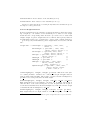
E is controlled by a very wide range of parameters. However, if you do not
want to bother with the details, you can leave configuration for a problem to
the prover. To use this feature, use the following command line options:
--autosat
--auto
--memory-limit=xx
Choose a literal selection strategy, a clause evaluation heuristic, and a term ordering automagically (based on problem features).
As --auto, but add heuristic specification pruning using one of several instantiation of the SInE
algorithm [HV11] for large specifications.
Tell the prover how much memory (measured in
MB) to use at most. In automatic mode E will optimize its behaviour for this amount (32 MB will
work, 128 MB is reasonable, 1024 MB is what I
use. More is better 1 , but if you go over your physical memory, you will probably experience very
heavy swapping.).
Example:
If you happen to have a workstation with 64 MB RAM2 , the
following command is reasonable:
eprover --auto --memory-limit=48 PUZ031-1+rm_eq_rstfp.lop
1 Emphasis
2 Yes,
added for E 0.7 and up, which globally cache rewrite steps.
this is outdated. If it still applies to you, get a new computer! It will still work ok,
though.
4
If you use problems in the current version of the TPTP language, you should
also add the option --tptp3-format (or only --tptp3-in if you like the traditional output more).
This documentation will probably lag behind the development of the latest
version of the prover for quite some time. To find out more about the options
available, type eprover --help (or consult the source code included with the
distribution).
5
Chapter 3
Calculus and Proof
Procedure
E is a purely equational theorem prover, based on ordered paramodulation and
rewriting. As such, it implements an instance of the superposition calculus
described in [BG94]. We have extended the calculus with some stronger contraction rules and a more general approach to literal selection. The core proof
procedure is a variant of the given-clause algorithm.
However, before proof search in clause normal form (CNF) begins, various
transformations can be applied to the input problem. In particular, E processes
not only clausal problems, but can read full first order format, including a rich
set of formula roles, logical operators and quantors. This format is reduced
to clause normal form in a way that the CNF is unsatisfiable if and only if
the original problem is provable (if an explicit conjecture is given) or itself
unsatisfiable.
3.1
Calculus
Term(F, V ) denotes the set of (first order) terms over a finite set of function
symbols F (with associated arities) and an enumerable set of variables V . We
write t|p to denote the subterm of t at a position p and write t[p ← t0 ] to
denote t with t|p replaced by t0 . An equation s ' t is an (implicitly symmetrical)
pair of terms. A positive literal is an equation s ' t, a negative literal is a
˙ to denote an arbitrary literal1 Literals
negated equation s 6' t. We write s't
can be represented as multi-sets of multi-sets of terms, with s ' t represented
1 Non-equational literals are encoded as equations or disequations P (t , . . . , t )'>.
In this
n ˙
1
case, we treat predicate symbols as special function symbols that can only occur at the topmost positions and demand that atoms (terms formed with a top predicate symbol) cannot
be unified with a first-order variable from V , i.e. we treat normal terms and predicate terms
as two disjoint sorts. We sometimes write the literal P (t1 , . . . , tn ) ' > as P (t1 , . . . , tn ) and
P (t1 , . . . , tn ) 6' > as ¬P (t1 , . . . , tn ) for simplicity.
6
as {{s}, {t}} and s 6' t represented as {{s, t}}. A ground reduction ordering
> is a Noetherian partial ordering that is stable w.r.t. the term structure and
substitutions and total on ground terms. > can be extended to an ordering >l
on literals by comparing the multi-set representation of literals with >>>> (the
multi-set-multi-set extension of >).
Clauses are multi-sets of literals. They are usually represented as disjunc˙ 1 ∨ s2 't
˙ 2 . . . ∨ sn 't
˙ n . We write Clauses(F , P , V ) to denote
tions of literals, s1 't
the set of all clauses with function symbols F , predicate symbols P and variable
V . If C is a clause, we denote the (multi-)set of positive literals in C by C + and
the (multi-)set of negative literals in C by C −
The introduction of an extended notion of literal selection has improved the
performance of E significantly. The necessary concepts are explained in the
following.
Definition 3.1.1 (Selection functions)
sel : Clauses(F , P , V ) → Clauses(F , P , V ) is a selection function, if it has the
following properties for all clauses C:
• sel (C) ⊆ C.
• If sel (C) ∩ C − = ∅, then sel (C) = ∅.
We say that a literal L is selected (with respect to a given selection function)
in a clause C if L ∈ sel (C).
J
We will use two kinds of restrictions on deducing new clauses: One induced
by ordering constraints and the other by selection functions. We combine these
in the notion of eligible literals.
Definition 3.1.2 (Eligible literals)
Let C = L ∨ R be a clause, let σ be a substitution and let sel be a selection
function.
• We say σ(L) is eligible for resolution if either
– sel (C) = ∅ and σ(L) is >L -maximal in σ(C) or
– sel (C) 6= ∅ and σ(L) is >L -maximal in σ(sel C) ∩ C − ) or
– sel (C) 6= ∅ and σ(L) is >L -maximal in σ(sel (C) ∩ C + )).
• σ(L) is eligible for paramodulation if L is positive, sel (C) = ∅ and σ(L) is
strictly >L -maximal in σ(C).
J
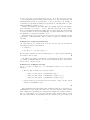
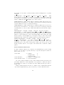
The calculus is represented in the form of inference rules. For convenience, we
distinguish two types of inference rules. For generating inference rules, written
with a single line separating preconditions and results, the result is added to
the set of all clauses. For contracting inference rules, written with a double
line, the result clauses are substituted for the clauses in the precondition. In
7
the following, u, v, s and t are terms, σ is a substitution and R, S and T are
(partial) clauses. p is a position in a term and λ is the empty or top-position.
D ⊆ F is a set of unused constant predicate symbols. Different clauses are
assumed to not share any common variables.
Definition 3.1.3 (The inference system SP)
Let > be a total simplification ordering (extended to orderings >L and >C
on literals and clauses), let sel be a selection function, and let D be a set of
fresh propositional constants. The inference system SP consists of the following
inference rules:
• Equality Resolution:
(ER)
u 6' v ∨ R
σ(R)
if σ = mgu(u, v) and σ(u 6'
v) is eligible for resolution.
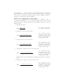
• Superposition into negative literals:
(SN)
if σ = mgu(u|p , s), σ(s) 6<
σ(t), σ(u) 6< σ(v), σ(s ' t)
is eligible for paramodulation, σ(u 6' v) is eligible for
resolution, and u|p ∈
/ V.
s ' t ∨ S u 6' v ∨ R
σ(u[p ← t] 6' v ∨ S ∨ R)
• Superposition into positive literals:
(SP)
if σ = mgu(u|p , s), σ(s) 6<
σ(t), σ(u) 6< σ(v), σ(s ' t)
is eligible for paramodulation, σ(u 6' v) is eligible for
resolution, and u|p ∈
/ V.
s't ∨ S u'v ∨ R
σ(u[p ← t] ' v ∨ S ∨ R)
• Simultaneous superposition into negative literals
(SSN)
s ' t ∨ S u 6' v ∨ R
σ(u[up ← t] 6' v ∨ S ∨ R)
if σ = mgu(u|p , s), σ(s) 6<
σ(t), σ(u) 6< σ(v), σ(s ' t)
is eligible for paramodulation, σ(u 6' v) is eligible for
resolution, and u|p ∈
/ V.
This inference rule is an alternative to (SN) that performs better in practice.
• Simultaneous superposition into positive literals
(SSP)
if σ = mgu(u|p , s), σ(s) 6<
σ(t), σ(u) 6< σ(v), σ(s ' t)
is eligible for paramodulation, σ(u 6' v) is eligible for
resolution, and u|p ∈
/ V.
s't ∨ S u'v ∨ R
σ(u[up ← t] ' v ∨ S ∨ R)
8
This inference rule is an alternative to (SP) that performs better in practice.
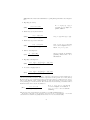
• Equality factoring:
(EF)
if σ = mgu(s, u), σ(s) 6>
σ(t) and σ(s ' t) eligible for
paramodulation.
s't ∨ u'v ∨ R
σ(t 6' v ∨ u ' v ∨ R)
• Rewriting of negative literals:
(RN)
s ' t u 6' v ∨ R
if u|p = σ(s) and σ(s) > σ(t).
s ' t u[p ← σ(t)] 6' v ∨ R
• Rewriting of positive literals 2 :
(RP)
if u|p = σ(s), σ(s) > σ(t), and
if u ' v is not eligible for resolution or u 6> v or p 6= λ.
s't u'v ∨ R
s ' t u[p ← σ(t)] ' v ∨ R
• Clause subsumption:
(CS)
C
where C and R are arbitrary
(partial) clauses and σ is a
substitution.
σ(C ∨ R)
C
• Equality subsumption:
(ES)
s ' t u[p ← σ(s)] ' u[p ← σ(t)] ∨ R
s't
• Positive simplify-reflect3 :
(PS)
s ' t u[p ← σ(s)] 6' u[p ← σ(t)] ∨ R
s't
R
2 A stronger version of (RP) is proven to maintain completeness for Unit and Horn problems and is generally believed to maintain completeness for the general case as well [Bac98].
However, the proof of completeness for the general case seems to be rather involved, as it requires a very different clause ordering than the one introduced [BG94], and we are not aware
of any existing proof in the literature. The variant rule allows rewriting of maximal terms of
maximal literals under certain circumstances:
(RP’)
s't
s't
if u|p = σ(s), σ(s) > σ(t) and if
u ' v is not eligible for resolution or
u 6> v or p 6= λ or σ is not a variable
renaming.
u'v ∨ R
u[p ← σ(t)] ' v ∨ R
This stronger rule is implemented successfully by both E and SPASS [Wei99].
3 In practice, this rule is only applied if σ(s) and σ(t) are >-incomparable – in all other
cases this rule is subsumed by (RN) and the deletion of resolved literals (DR).
9
• Negative simplify-reflect
(NS)
s 6' t σ(s) ' σ(t) ∨ R
s't
R
• Contextual (top level) simplify-reflect
(CSR)
.
σ(C ∨ R ∨ s = t)
σ(C ∨ R)
.
C ∨s=t
.
C ∨s=t
.
where s = t is the negation of
.
s = t and σ is a substitution
• Tautology deletion:
(TD)
C
if C is a tautology4
• Deletion of duplicate literals:
(DD)
s't ∨ s't ∨ R
s't ∨ R
• Deletion of resolved literals:
(DR)
s 6' s ∨ R
R
• Destructive equality resolution:
(DE)
x 6' y ∨ R
if x, y ∈ V, σ = mgu(x, y)
σ(R)
• Contextual literal cutting:
(CLC)
˙
σ(C ∨ R ∨ s't)
˙
C ∨ s't
σ(C ∨ R)
˙
C ∨ s't
˙ is the negation of
where s't
˙ and σ is a substitution
s't
This rule is also known as subsumption resolution or clausal simplification.
4 This
rule can only be implemented approximately, as the problem of recognizing tautologies is only semi-decidable in equational logic. Current versions of E try to detect tautologies
by checking if the ground-completed negative literals imply at least one of the positive literals,
as suggested in [NN93].
10
• Condensing:
(CON)
l1 ∨ l2 ∨ R
if σ(l1 ) ≡ σ(l2 ) and σ(l1 ∨ R)
subsumes l1 ∨ l2 ∨ R
σ(l1 ∨ R)
• Introduce definition5
(ID)
if R and S do not share any
variables, d ∈ D has not been
used in a previous definition
and R does not contain any
symbol from D
R∨S
d∨R
¬d ∨ S
• Apply definition
(AD)
if σ is a variable renaming, R
and S do not share any variables, d ∈ D and R does not
contain any symbol from D
σ(d ∨ R) R ∨ S
σ(d ∨ R) ¬d ∨ S
We write SP(N ) to denote the set of all clauses that can be generated with one
generating inference from I on a set of clauses N , DSP to denote the set of all
SP-derivations, and DSP to denote the set of all finite SP-derivations.
J
As SP only removes clauses that are composite with respect to the remaining
set of clauses, the calculus is complete. For the case of unit clauses, it degenerates into unfailing completion [BDP89] as implemented in DISCOUNT. E can
also simulate the positive unit strategy for Horn clauses described in [Der91]
using appropriate selection functions.
Contrary to e.g. SPASS, E does not implement special rules for non-equational literals or sort theories. Non-equational literals are encoded as equations
and dealt with accordingly.
3.2
Preprocessing
Axiom Filtering
Real-life axiom sets have grown steadily over the last years. One increasing
application for deduction is e.g. the answering of questions based on large
common-sense ontologies. Such specifications can contain from several thousand
to several million input axioms, only a small part of which are necessary for any
given query.
5 This rule is always exhaustively aplied to any clause, leaving n split-off clauses and one
final link clause of all negative propositions.
11
To avoid swamping the inference engine with most likely irrelevant facts, E
implements two different filtering mechanisms. Both start with the conjecture,
select facts that are likely connected to the conjecture, and then recursively
apply this process again.
• Classical relevancy pruning starts with the function and predicate symbols
in the goal. Every axioms that shares such a symbol is considered relevant. Symbols in selected axioms become relevant, and so become all their
function symbols. The process is then repeated for a selected number of
iterations. The option --rel-pruning-level determines how many iterations are performed. Relevance pruning is complete in the non-equational
case if allowed to reach a fixed point. It only provides a relatively coarse
measure, however.
• More fine-grained control is offered by the SInE method [HV11]. SInE
does not consider all symbols in already selected clauses and formulas to
be relevant, but defines a D-relation that determines which symbols to
consider relevant. E implements a frequency-based D-relation: in every
clause or formula, the least frequently occurring symbols are considered
relevant.
SInE in E is controlled via the option --sine. It takes as its argument
either the name of a predefined SInE filter specification, or a newly defined
strategy. The default is equivalent to --sine=Auto and will automatically
determine if axiom filtering should be applied, and if yes, which filter
should be applied. Filter selection is based on a number of features of
the problem specification, and on performance of different filters on the
TPTP problem library.
A SInE-Filter for E is specified as follows:
<sine-filter> ::= GSinE(<g-measure>,
hypos|nohypos,
<benvolvence>,
<generosity>,
<rec-depth>,
<set-size>,
<set-fraction [,
addnosymb|ignorenosymb])
– <g-measure> is the generality measure. Currently, CountFormulas
and CountTerms are supported.
– hypos or nohypos determines if clauses and formulas of type hypothesis
are used as additional seeds for the analysis.
– <benevolence> is a floating point value that determines how much
more general a function symbol in a clause or formula is allowed
to be relative to the least general one to be still considered for the
D-relation.
12
– <generosity> is an integer count and determines how many symbols
are maximally considered for the D-relation of each clause or formula.
– <rec-depth> determines the maximal number of iterations of the
selection algorithm.
– <set-size> gives an absolute upper bound for the number of clauses
and formulas selected.
– set-fraction gives a relative size (which fraction of clauses/formulas)
will be at most selected
– Finally, the optional last argument determines if clauses or formulas
which do not contain any function- or predicate symbols pass the
filter. This is a rare occurence, so the effect is minor in either case.
Clausification
E converts problems in full FOF into clause normal form using a slightly simplified version of the algorithm described by Nonnengart and Weidenbach [NW01].
E’s algorithm has the following modifications:
• E supports the full set of first-order connectives defined in the TPTP-3
language.
• E is more eager about introducing definitions to keep the CNF from
exponential explosion. E will introduce a definition for a sub-formula,
if it can determine that it will be duplicated more than a given number of times in the naive output. The limit can be set with the option
--definitional-cnf. E will reuse definitions generated for one input formula for syntactically identical formulae in other formulas with the same
specification.
• E supports mini-scoping, but not the more advanced forms of Skolemization.
It is possible to use E as a clausifier only. When given the --cnf option, E
will just perform clausification and print the resulting clause set.
Equational Definition unfolding
Equational definitions are unit clauses of the form f (X1 , . . . , Xn ) = t, where f
does not occur in t, and all variables in t are also in f . In this case, we can
completely replace all occurrences of f by the properly instantiated t. This
reduces the size of the search space, but can increase the size of the input
specification. In particular in the case of nested occurrences of f , this increase
can be significant.
E controls equational definition unfolding with the following options:
--eq-unfold-limit=<arg> limits unfolding (and removing) of equational
definitions to those where the expanded definition is at most the given limit
bigger (in terms of standard term weight) than the defined term.
13
--eq-unfold-maxclauses=<arg> inhibits unfolding of equational definitions
if the problem has more than the stated limit of clauses.
--no-eq-unfolding disables equational definition unfolding completely.
Presaturation Interreduction
If the option --presat-simplify is set, E will perform an inital interreduction
of the clause set. It will exhaustively apply simplifying inferences by running
its main proof procedure while disabling generating inferences.
Some problems can be solved purely by simplification, without the need for
deducing new clauses via the expensive application of the generating inference
rules, in particularly paramodulation/superposition. Moreover, exhaustive application of simplifying inferences can reduce redundancy in the specification
and allows all input clauses to be evaluated under the same initial conditions.
On the down side, a complete interreduction of the input problem can take
significant time, especially for large specifications.
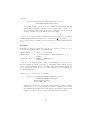
3.3
Proof Procedure
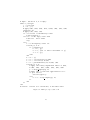
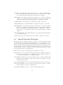
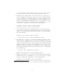
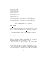
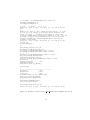
Fig. 3.1 shows a (slightly simplified) pseudocode sketch of the quite straightforward proof procedure of E. The set of all clauses is split into two sets, a set P of
processed clauses and a set U of unprocessed clauses. Initially, all input clauses
are in in U, and P is empty. The algorithm selects a new clause (sometimes called
the given clause) from U, simplifies it w.r.t. to P, then uses it to back-simplify
the clauses in P in turn. It then performs equality factoring, equality resolution
and superposition between the selected clause and the set of processed clauses.
The generated clauses are added to the set of unprocessed clauses. The process
stops when the empty clause is derived or no further inferences are possible.
The proof search is controlled by three major parameters: The term ordering
(described in section 4.2), the literal selection function, and the order in which
the select operation selects the next given clause to process.
E implements two different classes of term orderings, lexicographic term orderings and Knuth-Bendix orderings. A given ordering is determined by instantiating one of the classes with a variety of parameters (described in section 4.2).
Literal selection currently is done according to one of more than 50 predefined functions. Section 4.3 describes this feature.
Clause selection is determined by a heuristic evaluation function, which conceptually sets up a set of priority queues and a weighted round robin scheme
that determines from which queue the next clause is to be picked. The order
within each queue is determined by a priority function (which partitions the
set of unprocessed clauses into one or more subsets) and a heuristic evaluation
function, which assigns a numerical rating to each clause. Section 4.1 describes
the user interface to this mechanism.
14
# Input: Axioms in U, P is empty
while U 6= ∅ begin
c := select(U)
U := U \ {c}
# Apply (RN), (RP), (NS), (PS), (CSR), (DR), (DD), (DE)
simplify(c,P)
# Apply (CS), (ES), (TD)
if c is trivial or subsumed by P then
# Delete/ignore c
else if c is the empty clause then
# Success: Proof found
stop
else
T := ∅ # Temporary clause set
foreach p ∈ P do
if c simplifies p
P := P \ {p}
U := U \ {d|d is direct descendant of p}
T := T ∪ {p}
done
end
P := P ∪ {c}
T := T ∪ e-resolvents(c) # (ER)
T := T ∪ e-factors(c) # (EF)
T := T ∪ paramodulants(c,P) # (SN), (SP)
foreach p ∈ T do
# Apply efficiently implemented subset of (RN),
# (RP), (NS), (PS), (CSR), (DR), (DD), (DE)
p := cheap simplify(p, P)
# Apply (TD) or efficient approximation of it
if p is trivial
# Delete/ignore p
else
U := U ∪ cheap simplify(p, P)
fi
end
fi
end
# Failure: Initial U is satisfiable, P describes model
Figure 3.1: Main proof procedure of E
15
Chapter 4
Controlling the Proof
Search
This section describes some of the different options available to control the search
of the main proof procedure. The three most important choice points in the
proof search are the choice of term ordering, the selection of the given clause for
any iteration of the main loop, and the (optional) selection of inference literals.
In addition to these major choice points, there are a large number of additional
selections of lesser, but not insigificant importance.
4.1
Search Control Heuristics
Search control heuristics define the order in which the prover considers newly
generated clauses. A heuristic is defined by a set of clause evaluation functions
and a selection scheme which defines how many clauses are selected according
to each evaluation function. A clause evaluation function consists of a priority
function and an instance of a generic weight function.
Priority functions
Priority functions define a partition on the set of clauses. A single clause evaluation consists of a priority (which is the first selection criteria) and an evaluation.
Priorities are usually not suitable to encode heuristical control knowledge, but
rather are used to express certain elements of a search strategy, or to restrict the
effect of heuristic evaluation functions to certain classes of clauses. It is quite
trivial to add a new priority function to E, so at any time there probably exist
a few not yet documented here.
Syntactically, a large subset of currently available priority functions is described by the following rule:
<prio-fun> ::= PreferGroundGoals ||
16
PreferUnitGroundGoals ||
PreferGround ||
PreferNonGround ||
PreferProcessed ||
PreferNew ||
PreferGoals ||
PreferNonGoals ||
PreferUnits ||
PreferNonUnits ||
PreferHorn ||
PreferNonHorn ||
ConstPrio ||
ByLiteralNumber ||
ByDerivationDepth ||
ByDerivationSize ||
ByNegLitDist ||
ByGoalDifficulty ||
SimulateSOS||
PreferHorn||
PreferNonHorn||
PreferUnitAndNonEq||
DeferNonUnitMaxEq||
ByCreationDate||
PreferWatchlist||
DeferWatchlist
The priority functions are interpreted as follows:
PreferGroundGoals: Always prefer ground goals (all negative clauses without
variables), do not differentiate between all other clauses.
PreferUnitGroundGoals: Prefer unit ground goals.
PreferGround: Prefer clauses without variables.
PreferNonGround: Prefer clauses with variables.
PreferProcessed: Prefer clauses that have already been processed once and
have been eliminated from the set of processed clauses due to interreduction (forward contraction).
PreferNew: Prefer new clauses, i.e. clauses that are processed for the first time.
PreferGoals: Prefer goals (all negative clauses).
PreferNonGoals: Prefer non goals, i.e. facts with at least one positive literal.
PreferUnits: Prefer unit clauses (clauses with one literal).
PreferNonUnits: Prefer non-unit clauses.
17
PreferHorn: Prefer Horn clauses (clauses with no more than one positive literals).
PreferNonHorn: Prefer non-Horn clauses.
ConstPrio: Assign the same priority to all clauses.
ByLiteralNumber: Give a priority according to the number of literals, i.e. always prefer a clause with fewer literals to one with more literals.
ByDerivationDepth: Prefer clauses which have a short derivation depth, i.e.
give a priority based on the length of the longest path from the clause to
an axiom in the derivation tree. Counts generating inferences only.
ByDerivationSize: Prefer clauses which have been derived with a small number of (generating) inferences.
ByNegLitDist: Prefer goals to non-goals. Among goals, prefer goals with fewer
literals and goals with ground literals (more exactly: the priority is increased by 1 for a ground literal and by 3 for a non-ground literal. Clauses
with lower values are selected before clauses with higher values).
ByGoalDifficulty: Prefer goals to non-goals. Select goals based on a simple
estimate of their difficulty: First unit ground goals, then unit goals, then
ground goals, then other goals.
SimulateSOS: Use the priority system to simulate Set-Of-Support. This prefers
all initial clauses and all Set-Of-Support clauses. Some non-SOS-clauses
will be generated, but not selected for processing. This is neither well
tested nor a particularly good fit with E’s calculus, but can be used as
one among many heuristics. If you try a pure SOS strategy, you also should
set --restrict-literal-comparisons and run the prover without literal
selection enabled.
PreferHorn: Prefer Horn clauses (note: includes units).
PreferNonHorn: Prefer non-Horn clauses.
PreferUnitAndNonEq: Prefer all unit clauses and all clauses without equational
literal. This was an attempt to model some restricted calculi used e.g. in
Gandalf [Tam97], but did not quite work out.
DeferNonUnitMaxEq: Prefer everything except for non-unit clauses with a maximal equational literal (“Don’t paramodulate if its to expensive”). See
above, same result.
ByCreationDate: Return the creation date of the clause as priority. This imposes a FIFO equivalence class on clauses. Clauses generated from the
same given clause are grouped together (and can be ordered with any
evaluation function among each other).
18
PreferWatchlist Prefer clauses on the watchlist (see 4.4).
DeferWatchlist Defer clauses on the watchlist (see above).
Please note that careless use of certain priority functions can make the prover
incomplete for the general case.
Generic Weight Functions
Generic weight functions are templates for functions taking a clause and returning a weight (i.e. an estimate of the usefulness) for it, where a lower weight
means that the corresponding clause should be processed before a clause with
a higher weight. A generic weight function is combined with a priority function
and instantiated with a set of parameters to yield a clause evaluation function.
You can specify an instantiated generic weight function as described in this
rule1 :
<weight-fun> ::= Clauseweight ’(’ <prio-fun> ’, <int>, <int>,
<float> ’)’
Refinedweight ’(’ <prio-fun> ’, <int>, <int>,
<float>, <float>, <float> ’)’
Orientweight ’(’ <prio-fun>, <int>, <int>,
<float>, <float>, <float> ’)’
Simweight ’(’ <prio-fun>, <float>, <float>,
<float>, <float> ’)’
FIFOWeight ’(’ <prio-fun> ’)’
LIFOWeight ’(’ <prio-fun> ’)’
FunWeight ’(’ <prio-fun> ’, <int>, <int>,
<float>, <float>, <float>
(, <fun> : <posint> )* ’)’
SymOffsetWeight ’(’ <prio-fun> ’, <int>, <int>,
<float>, <float>, <float>
(, <fun> : <int> )* ’)’
||
||
||
||
||
||
||
Clauseweight(prio, fweight, vweight, pos mult): This is the basic symbol counting heuristic. Variables are counted with weight vweight, function
symbols with weight fweight. The weight of positive literals is multiplied by
pos mult before being added into the final weight.
Refinedweight(prio, fweight, vweight, term pen, lit pen, pos mult):
This weight function is very similar to the first one. It differs only in that it
takes the effect of the term ordering into account. In particular, the weight of
a term that is maximal in its literal is multiplied by term pen, and the weight
of maximal literals is multiplied by lit pen.
Orientweight(prio, fweight, vweight, term pen, lit pen, pos mult):
This weight function is a slight variation of Refinedweight(). In this case,
1 Note
that there now are many additional generic weight functions not yet documented.
19
the weight of both terms of an unorientable literal is multiplied by a penalty
term pen.
Simweight(prio, equal weight, vv clash, vt clash, tt clash):
This
weight function is intended to return a low weight for literals in which the
two terms are very similar. It does not currently work very well even for unit
clauses – RTFS (in <che simweight.c>) to find out more.
FIFOWeight(prio): This weight function assigns weights that increase in a
strictly monotonic manner, i.e. it realizes a first-in/first-out strategy if used all
by itself. This is the most obviously fair strategy.
LIFOWeight(prio): This weight function assigns weights that decrease in a
strictly monotonic manner, i.e. it realizes a last-in/first-out strategy if used all
by itself (which, of course, would be unfair and result in an extremely incomplete
prover).
FunWeight(prio, fweight, vweight, term pen, lit pen, pos mult,
fun:fweight ...): This evaluation function is a variant of Refinedweight.
The first 6 parameter are identical in meaning. The function takes an arbitrary
number of extra parameters of the form fun:fweight, where fun is any valid
function symbol, and fweight is a non-negative integer. The extra weight
assignments will overwrite the default weight for the listed function symbol.
SymOffsetWeight(prio, fweight, vweight, term pen, lit pen,
pos mult, fun:fweight ...):
This evaluation function is similar to
FunWeight. The first 6 parameter are identical in meaning. The extra
arguments allow both positive and negative values, and are used as once-off
weight modifiers added to the weight of all clauses that contain the defined
symbol.
Clause Evaluation Functions
A clause evaluation function is constructed by instantiating a generic weight
function. It can either be specified directly, or specified and given a name for
later reference at once:
<eval-fun>
::= <ident>
||
<weight-fun>
||
<eval-fun-def>
<eval-fun-def>
::= <ident> = <weight-fun>
<eval-fun-def-list> ::= <eval-fun-def>*
Of course a single identifier is only a valid evaluation function if it has been
previously defined in a <eval-fun-def>. It is possible to define the value of
an identifier more than once, in which case later definitions take precedence to
former ones.
Clause evaluation functions can be be defined on the command line with the
-D (--define-weight-function) option, followed by a <eval-fun-def-list>.
20
Example:
eprover -D"ex1=Clauseweight(ConstPrio,2,1,1) \
ex2=FIFOWeight(PreferGoals)" ...
sets up the prover to know about two evaluation function ex1 and ex2
(which supposedly will be used later on the command line to define one or
more heuristics). The double quotes are necessary because the brackets
and the commas are special characters for most shells
There are a variety of clause evaluation functions predefined in the variable
DefaultWeightFunctions, which can be found in che proofcontrol.c. See
also sections 4.4 and 4.5, which cover some of the more complex weight functions
of E.
Heuristics
A heuristic defines how many selections are to be made according to one of
several clause evaluation functions. Syntactically,
<heu-element>
<heuristic>
::= <int> ’*’ <eval-fun>
::= ’(’ <heu-element> (,<heu-element>)* ’)’ ||
<ident>
<heuristic-def> ::= <ident> = <heuristic> ||
<heuristic>
As above, a single identifier is only a valid heuristic if it has been defined in <heuristic-def> previously. A <heuristic-def> which degenerates to a simple heuristic defines a heuristic with name Default (which the
prover will automatically choose if no other heuristic is selected with the -x
(--expert-heuristic).
Example: To continue the above example,
eprover -D"ex1=Clauseweight(ConstPrio,2,1,1) \
ex2=FIFOWeight(PreferGoals)"
-H"new=(3*ex1,1*ex2)" \
-x new LUSK3.lop
will run the prover on a problem file named LUSK3.lop with a heuristic
that chooses 3 out of every 4 clauses according to a simple symbol counting heuristic and the last clause first among goals and then among other
clauses, selecting by order of creation in each of these two classes.
21
4.2
Term Orderings
E currently supports two families of orderings: The Knuth-Bendix-Ordering
(KBO), which is used by default, and the Lexicographical Path Ordering (LPO).
The KBO is weight-based and uses a precedence on function symbols to break
ties. Consequently, to specify a concrete KBO, we need a weight function that
assigns a weight to all function symbols, and a precedence on those symbols.
The LPO is based on a lexicographic comparison of symbols and subterms,
and is fully specified by giving just a precedence.
Currently it is possible to explicitly specify an arbitrary (including incomplete or empty) precedence, or to use one of several precedence generating
schemes. Similarly, there is a number of predefined weight function and the
ability to assign arbitrary weights to function and predicate symbols.
The simplest way to get a reasonable term ordering is to specify automatic
ordering selection using the -tAuto option.
Options controlling the choice of term ordering:
22
-term-ordering=<arg>
-t<arg>
Select a term ordering class (or automatic selection). Supported arguments are at least LPO, LPO4 (for a much faster
new implementation of LPO), KBO, and Auto. If Auto is selected, all aspects of the term ordering are fixed, additional
options will be (or at least should be) silently ignored.
--order-precedence-generation=<arg>
-G <arg> Select a precedence generation scheme (see below).
--order-weight-generation=<arg>
-w <arg> Select a symbol weight function (see below).
--order-constant-weight=<arg>
-c <arg> Modify any symbol weight function by assigning a special
weight to constant function symbols.
--precedence[=<arg>]
Describe a (partial) precedence for the term ordering. The argument is a comma-separated list of precedence chains, where
a precedence chain is a list of function symbols (which all
have to appear in the proof problem), connected by >, <, or
= (to denote equivalent symbols). If this option is used in
connection with --order-precedence-generation, the partial ordering will be completed using the selected method,
otherwise the prover runs with a non-ground-total ordering.
The option without the optional argument is equivalent to
--precedence= (the empty precedence). There is a drawback
to using --precedence: Normally, total precedences are represented by mapping symbols to a totally ordered set (small
integers) which can be compared using standard machine instructions. The used data structure is linear in the number n
of function symbols. However, if --precedence is used, the
prover allocates (and completes) a n × n lookup table to efficiently represent an arbitrary partial ordering. If n is very big,
this matrix takes up significant space, and takes a long time
to compute in the first place. This is unlikely to be a problem
unless there are at least hundreds of symbols.
--order-weights=<arg>
Give explicit weights to function symbols. The argument syntax is a comma-separated list of items of the form f:w, where
f is a symbol from the specification, and w is a non-negative
integer. Note that at best very simple checks are performed,
so you can specify weights that do not obey the KBO weight
constraints. Behaviour in this case is undefined. If all your
weights are positive, this is unlikely to happen.
Since KBO needs a total weight function, E always uses a
weight generation scheme in addition to the user-defined options. You may want to use -wconstant for predictable
behaviour.
23
--lpo-recursion-limit[=<arg>]
Limits the recursion depth of LPO comparison. This is useful
in rare cases where very large term comparisons can lead to
stack overflow issues. It does not change completeness, but
may lead to unnecessary inferences in rare cases (Note: By
default, recursion depth is limited to 1000. To get effectively
unlimited recursion depth, use this option with an outrageously
large argument. Don’t forget to increase process stack size with
limit/ulimit from your favourite shell).
Precedence Generation Schemes
Precedence generation schemes are based on syntactic features of the symbol and the input clause set, like symbol arity or number of occurrences in
the formula. At least the following options are supported as argument to
--order-precedence-generation:
unary first: Sort symbols by arity, with the exception that unary symbols
come first. Frequency is used as a tie breaker (rarer symbols are greater).
unary freq: Sort symbols by frequency (rarer symbols are bigger), with the
exception that unary symbols come first. Yes, this should better be named
unary invfreq for consistency, but is not. . .
arity: Sort symbols by arity (symbols with higher arity are larger).
invarity: Sort symbols by arity (symbols with higher arity are smaller).
const max: Sort symbols by arity (symbols with higher arity are larger), but
make constants the largest symbols. This is allegedly used by SPASS [Wei01]
in some configurations.
const min: Sort symbols by arity (symbols with higher arity are smaller), but
make constants the smallest symbols. Provided for reasons of symmetry.
freq: Sort symbols by frequency (frequently occurring symbols are larger). Arity is used as a tie breaker.
invfreq: Sort symbols by frequency (frequently occurring symbols are smaller).
In our experience, this is one of the best general-purpose precedence generation schemes.
invfreqconstmin: Same as invfreq, but make constants always smaller than
everything else.
invfreqhack: As invfreqconstmin, but unary symbols with maximal frequency
become largest.
24
Weight Generation Schemes
Weight generation schemes are based on syntactic features of the symbol and
the input clause set, or on the predefined precedence. The following options are
available for --order-weight-generation.
firstmaximal0: Give the same arbitrary (positive) weight to all function symbols except to the first maximal one encountered (order is arbitrary),
which is given weight 0.
arity: Weight of a function symbol f |n is n + 1, i.e. its arity plus one.
aritymax0: As arity, except that the first maximal symbol is given weight 0.
modarity: Weight of a function symbol f |n is n+c, where c is a positive constant
(W TO BASEWEIGHT, which has been 4 since the dawn of time).
modaritymax0: As modarity, except that the first maximal symbol is given
weight 0.
aritysquared: Weight of a symbol f |n is n2 + 1.
aritysquaredmax0: As aritysquared, except that the first maximal symbol is
given weight 0.
invarity: Let m be the largest arity of any symbol in the signature. Weight
of a symbol f |n is m − n + 1.
invaritymax0: As invarity, except that the first maximal symbol is given
weight 0.
invaritysquared: Let m be the largest arity of any symbol in the signature.
Weight of a symbol f |n is m2 − n2 + 1.
invaritysquaredmax0: As invaritysquared, except that the first maximal
symbol is given weight 0.
precedence: Let < be the (pre-determined) precedence on function symbols F
in the problem. Then the weight of f is given by |g|g < f |+1 (the number
of symbols smaller than f in the precedence increased by one).
invprecedence: Let < be the (pre-determined) precedence on function symbols
F in the problem. Then the weight of f is given by |g|f < g| + 1 (the
number of symbols larger than f in the precedence increased by one).
freqcount: Make the weight of a symbol the number of occurrences of that
symbol in the (potentially preprocessed) input problem.
invfreqcount: Let m be the number of occurrences of the most frequent symbol
in the input problem. The weight of f is m minus he number of occurrences
of f in the input problem.
25
freqrank: Sort all function symbols by frequency of occurrence (which induces
a total quasi-ordering). The weight of a symbol is the rank of it’s equivalence class, with less frequent symbols getting lower weights.
invfreqrank: Sort all function symbols by frequency of occurrence (which induces a total quasi-ordering). The weight of a symbol is the rank of its
equivalence class, with less frequent symbols getting higher weights.
freqranksquare: As freqrank, but weight is the square of the rank.
invfreqranksquare: As invfreqrank, but weight is the square of the rank.
invmodfreqrank: Sort all function symbols by frequency of occurrence (which
induces a total quasi-ordering). The weight of an equivalence class is the
sum of the cardinality of all smaller classes (+1). The weight of a symbol
is the weight of its equivalence classes. Less frequent symbols get higher
weights.
invmodfreqrankmax0: As invmodfreqrank, except that the first maximal symbol is given weight 0.
constant: Give the same arbitrary positive weight to all function symbols.
4.3
Literal Selection Strategies
The superposition calculus allows the selection of arbitrary negative literals
in a clause and only requires generating inferences to be performed on these
literals. E supports this feature and implements it via manipulations of the
literal ordering. Additionally, E implements strategies that allow inferences into
maximal positive literals and selected negative literals. A selection strategy is
selected with the option --literal-selection-strategy. Currently, at least
the following strategies are implemented:
NoSelection: Perform ordinary superposition without selection.
NoGeneration: Do not perform any generating inferences. This strategy is not
complete, but applying it to a formula generates a normal form that does
not contain any tautologies or redundant clauses.
SelectNegativeLiterals: Select all negative literals. For Horn clauses, this
implements the maximal literal positive unit strategy [Der91] previously
realized separately in E.
SelectPureVarNegLiterals: Select the first negative literal of the form X ' Y .
SelectLargestNegLit: Select the largest negative literal (by symbol counting,
function symbols count as 2, variables as 1).
SelectSmallestNegLit: As above, but select the smallest literal.
26
SelectDiffNegLit: Select the negative literal in which both terms have the
largest size difference.
SelectGroundNegLit: Select the first negative ground literal for which the size
difference between both terms is maximal.
SelectOptimalLit: If there is a ground negative literal, select as in the case of
SelectGroundNegLit, otherwise as in SelectDiffNegLit.
Each of the strategies that do actually select negative literals has a corresponding counterpart starting with P that additionally allows paramodulation
into maximal positive literals2 .
Example: Some problems become a lot simpler with the correct strategy. Try
e.g.
eprover --literal-selection-strategy=NoSelection \
GRP001-1+rm_eq_rstfp.lop
eprover --literal-selection-strategy=SelectLargestNegLit \
GRP001-1+rm_eq_rstfp.lop
You will find the file GRP001-1+rm eq rstfp.lop in the E/PROVER directory.
As we aim at replacing the vast number of individual literal selection functions with a more abstract mechanism, we refrain from describing all of the currently implemented functions in detail. If you need information about the set
of implemented functions, run eprover -W none. The individual functions are
implemented and somewhat described in E/HEURISTICS/che litselection.h.
4.4
The Watchlist Feature
Since public release 0.81, E supports a watchlist. A watchlist is a user-defined set
of clauses. Whenever the prover encounters3 a clause that subsumes one or more
clauses from the watchlist, those clauses are removed from it. The saturation
process terminates if the watchlist is empty (or, of course, if a saturated state
or the empty clause have been reached).
There are two uses for a watchlist: To guide the proof search (using a heuristic that prefers clauses on the watchlist), or to find purely constructive proofs
for clauses on the watchlist.
If you want to guide the proof search, place clauses you believe to be important lemmata onto the watchlist. Also include the empty clause to make
2 Except for SelectOptimalLit, where the resulting strategy, PSelectOptimalLit will allow
paramodulation into positive literals only if no ground literal has been selected.
3 Clauses are checked against the watchlist after normalization, both when they are inserted
into U or if they are selected for processing.
27
sure that the prover will not terminate prematurely. You can then use a clause
selection heuristic that will give special consideration to clauses on the watchlist. This is currently supported via the priority functions PreferWatchlist
and DeferWatchlist. A clause evaluation function using PreferWatchlist
will always select clauses which subsume watchlist clauses first. Similarly, using
DeferWatchlist can be used to put the processing of watchlist clauses off.
There is a predefined clause selection heuristic UseWatchlist (select it with
-xUseWatchlist) that will make sure that watchlist clauses are selected relatively early. It is a strong general purpose heuristic, and will maintain completeness of the prover. This should allow easy access to the watchlist feature
even if you don’t yet feel comfortable with specifying your own heuristics.
To generate constructive proofs of clauses, just place them on the watch list
and select output level 4 or greater (see section 6.3). Steps affecting the watch
list will be marked in the PCL2 output file. If you use the eproof script for
proof output or run epclextract of your own, subproof for watchlist steps will be
automatically extracted.
Note that this forward reasoning is not complete, i.e. the prover may never
generate a given watchlist clause, even if it would be trivial to prove it via
refutation.
Options controlling the use of the watch list:
--watchlist=<arg>
Select a file containing the watch list
clauses. Syntax should be the same
syntax as your proof problem (E-LOP,
TPTP-1/2 or TPTP-3/TSTP). Just
write down a list of clauses and/or formulas.
--no-watchlist-simplification By default, watch list clauses are simplified with respect to the current set
P. Use this option to disable the feature.
4.5
Learning Clause Evaluation Functions
E can use a knowledge base generated by analyzing many successful proof attempts to guide its search, i.e. it can learn what kinds of clauses are likely to be
useful for a proof and which ones are likely superfluous. The details of the learning mechanism can be found in [Sch00, Sch01]. Essentially, an inference protocol
is analyzed, useful and useless clauses are identified and generalized into clause
patterns, and the resulting information is stored in a knowledge base. Later,
new clauses that match a pattern are evaluated accordingly.
Creating Knowledge Bases
An E knowledge base is a directory containing a number of files, storing both
the knowledge and configuration information. Knowledge bases are generated
28
with the tool ekb create. If no argument is given, ekb create will create a
knowledge base called E KNOWLEDGE in the current directory.
You can run ekb create -h for more information about the configuration.
However, the defaults are usually quite sufficient.
Populating Knowledge Bases
The knowledge base contains information gained from clausal PCL2 protocols
of E. In a first step, information from the protocol is abstracted into a more
compact form. A number of clauses is selected as training examples, and annotations about there role are computed. The result is a list of annotated clauses
and a list of the axioms (initial clauses) of the problem. This step can be
performed using the program direct examples4 .
In a second step, the collected information is integrated into the knowledge
base. For this purpose, the program ekb insert can be used. However, it is
probably more convenient to use the single program ekb ginsert, which directly
extracts all pertinent information from a PCL2 protocol and inserts it into a
designated knowledge base.
The program ekb delete will delete an example from a knowledge base.
This process is not particularly efficient, as the whole knowledge base is first
parsed.
Using Learned Knowledge
The knowledge in a knowledge base can be utilized by the two clause evaluation functions TSMWeight() and TSMRWeight(). Both compute a modification weight based on the learned knowledge, and apply it to a conventional
symbol-counting base weight (similar to Clauseweight() for TSMWeight() and
Refinedweight() for TSMWeight(). An example command line is:
eprover -x’(1*TSMWeight(ConstPrio, 1, 1, 2, flat, E KNOWLEDGE,
100000,1.0,1.0,Flat,IndexIdentity,100000,-20,20,-2,-1,0,2))’
There are also two fully predefined learning clause selection heuristics. Select them with -xUseTSM1 (for some influence of the learned knowledge) or
-xUseTSM2 (for a lot of influence of the learned knowledge).
4.6
4 The
Other Options
name is an historical accident and has no significance anymore
29
Chapter 5
Input Language
5.1
LOP
E natively uses E-LOP, a dialect of the LOP language designed for SETHEO.
At the moment, your best bet is to retrieve the LOP description from the E web
site [Sch12] and/or check out the examples available from it. LOP is very close
to Prolog, and E can usually read many fully declarative Prolog files if they do
not use arithmetic or rely on predefined symbols. Plain SETHEO files usually
also work very well. There are a couple of minor differences, however:
• equal() is an interpreted symbol for E. It normally does not carry any
meaning for SETHEO (unless equality axioms are added).
• SETHEO allows the same identifier to be used as a constant, a nonconstant function symbol and a predicate symbol. E encodes all of these
as ordinary function symbols, and hence will complain if a symbol is used
inconsistently.
• E allows the use of = as an infix symbol for equality. a=b is equivalent to
equal(a,b) for E.
• E does not support constraints or SETHEO build-in symbols. This should
not usually affect pure theorem proving tasks.
• E normally treats procedural clauses exactly as it treats declarative clauses.
Query clauses (clauses with an empty head and starting with ?-, e.g.
?-∼p(X), q(X). can optionally be used to define the a set of goal clauses
(by default, all negative clauses are considered to be goals). At the moment, this information is only used for the initial set of support (with
--sos-uses-input-types). Note that you can still specify arbitrary
clauses as query clauses, since LOP supports negated literals.
30
5.2
TPTP Format
The TPTP [Sut09] is a library of problems for automated theorem prover. Problems in the TPTP are written in TPTP syntax. There are two major versions
of the TPTP syntax, both of which are supported by E.
Version 21 of the TPTP syntax was used up for TPTP releases previous to
TPTP 3.0.0. The current version 3 of the TPTP syntax, described in [SSCG06],
covers both input problems and both proof and model output using one consistent formalism. It has been used as the native format for TPTP releases since
TPTP 3.0.0.
Parsing in TPTP format version 2 is enabled by the options --tptp-in,
tptp2-in, --tptp-format and --tptp2-format. The last two options also select TPTP 2 format for the output of normal clauses during and after saturation.
Proof output will be in PCL2 format, however.
TPTP syntax version 3 [SSCG06] is the currently recommended format. It is
supported by many provers, it is more consistent than the old TPTP language,
and it adds a number of useful features. E supports TPTP-3 syntax with the
options --tstp-in , tptp3-in, --tstp-format and --tptp3-format. The last
two options will also enable TPTP-3 format for proof output. Note that many of
E’s support tools still require PCL2 format. Various tools for processing TPTP3 proof format are available via the TPTP web-site, http://www.tptp.org.
In either TPTP format, clauses and formulas with TPTP type conjecture,
negated-conjecture, or question (the last two in TPTP-3 only) are considered goal clauses for the --sos-uses-input-types option.
1 Version 1 allowed the specification of problems in clause normal form only. Version 2 is a
conservative extension of version 1 and adds support for full first order formulas.
31
Chapter 6
Output. . . or how to
interpret what you see
E has several different output levels, controlled by the option -l or --output-level.
Level 0 prints nearly no output except for the result. Level 1 is intended to give
humans a somewhat readable impression of what is going on inside the inference engine. Levels 3 to 6 output increasingly more information about the inside
processes in PCL2 format. At level 4 and above, a (large) superset of the proof
inferences is printed. You can use the epclextract utility in E/PROVER/ to
extract a simple proof object.
In Level 0 and 1, everything E prints is either a clause that is implied by the
original axioms, or a comment (or, very often, both).
6.1
The Bare Essentials
In silent mode (--output-level=0, -s or --silent), E will not print any output
during saturation. It will print a one-line comment documenting the state of
the proof search after termination. The following possibilities exist:
• The prover found a proof. This is denoted by the output string
# Proof found!
• The problem does not have a proof, i.e. the specification is satisfiable (and
E can detect this):
# No proof found!
Ensuring the completeness of a prover is much harder than ensuring correctness. Moreover, proofs can easily be checked by analyzing the output
of the prover, while such a check for the absence of proofs is rarely possible.
32
I do believe that the current version of E is both correct and complete1
but my belief in the former is stronger than my belief in the later. . . ...
• A (hard) resource limit was hit. For memory this can be either due to a
per process limit (set with limit or the prover option --memory-limit),
or due to running out of virtual memory. For CPU time, this case is
triggered if the per process CPU time limit is reached and signaled to the
prover via a SIGXCPU signal. This limit can be set with limit or, more
reliable, with the option --cpu-limit. The output string is one of the
following two, depending on the exact reason for termination:
# Failure: Resource limit exceeded (memory)
# Failure: Resource limit exceeded (time)
• A user-defined limit was reached during saturation, and the saturation process was stopped gracefully. Limits include number of processed clauses,
number of total clauses, and cpu time (as set with --soft-cpu-limit).
The output string is
# Faiure: User resource limit exceeded!
. . . and the user is expected to know which limit he selected.
• By default, E is complete, i.e. it will only terminate if either the empty
clause is found or all clauses have been processed (in which case the processed clause set is satisfiable). However, if the option --delete-bad-limit
is given or if automatic mode in connection with a memory limit is used, E
will periodically delete clauses it deems unlikely to be processed to avoid
running out of memory. In this case, completeness cannot be ensured any
more. This effect manifests itself extremely rarely. If it does, E will print
the following string:
# Failure: Out of unprocessed clauses!
This is roughly equivalent to Otter’s SOS empty message.
• Finally, it is possible to chose restricted calculi when starting E. This is
useful if E is used as a normalization tool or as a preprocessor or lemma
generator. In this case, E will print a corresponding message:
# Clause set closed under restricted calculus!
1 Unless
the prover runs out of memory (see below), the user selects an unfair strategy (in
which case the prover may never terminate), or some strange and unexpected things happen.
33
6.2
Impressing your Friends
If you run E without selection an output level (or by setting it explicitly to
1), E will print each non-tautological, non-subsumed clause it processes as a
comment. It will also print a hash (’#’) for each clause it tries to process but
can prove to be superfluous.
This mode gives some indication of progress, and as the output is fairly
restricted, does not slow the prover down too much.
For any output level greater than 0, E will also print statistical information
about the proof search and final clause sets. The data should be fairly selfexplaining.
6.3
Detailed Reporting
At output levels greater that 1, E prints certain inferences in PCL2 format2 or
TPTP-3 output format. At level 2, it only prints generating inferences. At level
4, it prints all generating and modifying inferences, and at level 6 it also prints
PCL steps giving a lot of insight into the internal operation of the inference
engine. This protocol is fairly readable and, from level 4 on can be used to
check the proof with the utility checkproof provided with the distribution.
6.4
Requesting Specific Output
There are two additional kinds of information E can provide beyond the normal
output during proof search: Statistical information and final clause sets (with
additional information).
First, E can give you some technical information about the conditions it runs
under.
The option --print-pid will make E printing its process id as a comment,
in the format # Pid: XXX, where XXX is an integer number. This is useful if
you want to send signals to the prover (in particular, if you want to terminate
the prover) to control it from the outside.
The option -R (--resources-info) will make E print a summary of used
system resources after graceful termination:
#
#
#
#
User time
:
System time
:
Total time
:
Maximum resident set size:
0.010 s
0.020 s
0.030 s
0 pages
Most operating systems do not provide a valid value for the resident set size
and other memory-related resources, so you should probably not depend on the
last value to carry any meaningful information. The time information is required
by most standards and should be useful for all tested operating systems.
2 PCL2
is a proof output designed as a successor to PCL [DS94a, DS94b, DS96].
34
E can be used not only as a prover, but as a normalizer for formulae or as
a lemma generator. In this cases, you will not only want to know if E found a
proof, but also need some or all of the derived clauses, possibly with statistical
information for filtering. This is supported with the --print-saturated and
--print-sat-info options for E.
The option --print-saturated takes as its argument a string of letters,
each of which represents a part of the total set of clauses E knows about. The
following table contains the meaning of the individual letters:
e Processed positive unit clauses (Equations).
i Processed negative unit clauses (Inequations).
g Processed non-unit clauses (except for the empty clause,
which, if present, is printed separately). The above three
sets are interreduced and all selected inferences between
them have been computed.
E Unprocessed positive unit clauses.
I Unprocessed negative unit clauses.
G Unprocessed non-unit clause (this set may contain the
empty clause in very rare cases).
a Print equality axioms (if equality is present in the problem). This letter prints axioms for reflexivity, symmetry,
and transitivity, and a set of substitutivity axioms, one for
each argument position of every function symbol and predicate symbol.
A As a, but print a single substitutivity axiom covering all
positions for each symbol.
The short form, -S, is equivalent to --print-saturated=eigEIG. If the option --print-sat-info is set, then each of the clauses is followed by a comment
of the form # info(id, pd, pl, sc, cd, nl, no, nv). The following table
explains the meaning of these values:
id Clause ident (probably only useful internally)
pd Depth of the derivation graph for this clause
pl Number of nodes in the derivation grap
sc Symbol count (function symbols and variables)
cd Depth of the deepest term in the clause
nl Number of literals in the clause
no Number of variable occurences
nv Number of different variables
35
Chapter 7
Additional utilities
The E distribution contains a number of programs beyond the main prover.
The following sections contains a short description of the programs that are
reasonably stable. All of the utilities support the option --help to print a
description of the operation and all supported options.
7.1
Common options
All major programs in the E distribution share some common options. Some
more options are shared to the degree that they are applicable. The most
important of these shared options are listed in Table 7.1.
7.2
Grounding: eground
The Bernays-Sch¨
onfinkel class is a decidable fragment of first-order logic. Problems from this class can be clausified into clause normal form without nonconstant function symbols. This clausal class is effectively propositional (EPR),
since the Herbrand universe is finite. The program eground takes a problem
from the Bernays-Sch¨
onfinkel class, or an EPR clause normal form problem,
and tries to convert it into an equisatisfiable propositional problem. It does
so by clausification and instantiation of the the clausal problem. The resulting propositional problem can than be handed to a propositional reasoner (e.g.
Chaff [MMZ+ 01] or MiniSAT [ES04]). One pre-packaged system build on this
principles is GrAnDe [SS02].
Eground uses a number of techniques to reduce the number of instances
generated. The technical background is described in [Sch02a]. The program
can generate output in LOP, TPTP-2 and TPTP-3 format, but also directly in
the DIMACS format used by many propositional reasoners.
A typical command line for starting eground is:
eground --tptp3-in --dimacs
--split-tries=1
36
-h
--help
Print the help page for the program. This usually includes documentation for all options supported by the program.
-V
--version
Print the version number of the program. If you encounter bugs,
please check if updating to the latest version solves your problem.
Also, always include the output of this with all bug reports.
-v
--verbose[=level]
Make the program more verbose. Verbose output is written to
stterr, not the standard output, and will cover technical aspects.
Most programs support verbosity levels 0 (the default), 1, and 2,
with -v selecting level 1.
-s
--silent
Reduce output of the tool to a minimal.
-o<outfile>
--output-file=<outfile>
By default, most of the programs in the E distribution provide output
to stdout, i.e. usually to the controlling terminal. This option allows
the user to specify an output file.
--tptp2-in
--tptp2-out
--tptp2-format
--tptp3-in
--tptp3-out
--tptp3-format
Select TPTP formats for input and/or output. If you do not start
with an existing corpus, the recommended format is TPTP-3 syntax.
Figure 7.1: Common program options
37
--constraints <infile> -o <outfile>
7.3
Rewriting: enormalizer
The program enormalizer uses E’s shared terms, cached rewriting, and indexing to implement an efficient normalizer. It reads a set of rewrite rules and
computes the normal forms of a set of terms, clauses and formulas with respect
to that set of rewrite rules.
The rule set can be specified as a set of positive unit clauses and/or formulas
that clausify into unit clauses. Literals are taken as rewrite rules with the
orientation they are specified in the input. In particular, no term ordering is
applies, and neither termination nor confluence are ensured or verified. The
rewrite rules are applied exhaustively, but in an unspecified order. Subterms
are normalized in strict leftmost/innermost manner. In particular, all subterms
are normalized before a superterm is rewritten.
Supported formats are LOP, TPTP-2 and TPTP-3.
A typical command line for starting enormalizer is:
enormalizer --tptp3-in <rulefile> -t<termfile>
7.4
Multiple queries: e ltb runner
E is designed to handle individual proof problems, one at a time. For this
case, the prover has mechanism to handle even large specifications. However, in
cases where multiple queries or conjectures are posed against a large background
theory, even the parsing of the background theory may take up significant time.
E ltb runner has been developed to efficiently handle this situation. It can
read the background theory once, and then run E with additional axioms and
different conjectures against this background theory.
The program was originally designed for running sets of queries against large
theories in batch mode, but now also supports interactive queries. However,
the program is in a more prototypical state than most of the E distribution.
In particular, any syntax error in the input will cause the whole program to
terminate.
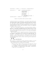
By default, it will process a batch specification file (see 7.4.2), which contains a specification of the background theory, some options, and (optionally) a
number of individual job requests. If used with the option --interactive, it
will enter interactive mode (7.4.3) after all batch jobs have been processed.
For every job, the program will use several different goal-directed pruning
strategies to extract likely useful axioms from the background theory. For each
of the pruned axiomatizations, e ltb runner will run E in automatic mode. If
one of the strategies succeeds, all running strategies will be terminated and the
result returned.
The program will run up to 8 strategies in parallel. Thus, it is best used on
a multi-core machine with sufficient amounts of memory.
38
% SZS start BatchConfiguration
division.category LTB.SMO
execution.order ordered
output.required Assurance
output.desired Proof Answer
limit.time.problem.wc 60
% SZS end BatchConfiguration
% SZS start BatchIncludes
include(’Axioms/CSR003+2.ax’).
include(’Axioms/CSR003+5.ax’).
% SZS end BatchIncludes
% SZS start BatchProblems
/Users/schulz/EPROVER/TPTP_5.4.0_FLAT/CSR083+3.p
/Users/schulz/EPROVER/TPTP_5.4.0_FLAT/CSR075+3.p
/Users/schulz/EPROVER/TPTP_5.4.0_FLAT/CSR082+3.p
/Users/schulz/EPROVER/TPTP_5.4.0_FLAT/CSR086+3.p
/Users/schulz/EPROVER/TPTP_5.4.0_FLAT/CSR091+3.p
/Users/schulz/EPROVER/TPTP_5.4.0_FLAT/CSR092+3.p
% SZS end BatchProblems
/Users/schulz/tmp/CSR083+3
/Users/schulz/tmp/CSR075+3
/Users/schulz/tmp/CSR082+3
/Users/schulz/tmp/CSR086+3
/Users/schulz/tmp/CSR091+3
/Users/schulz/tmp/CSR092+3
Figure 7.2: Example LTB batch specification file
7.4.1
Usage
E ltb runner relies on TPTP-3 include file syntax and semantics, and hence
will only (and implicitly) work with the TPTP-3 syntax. The main program
runs both eprover and epclextract as sub-processes. Unless these programs
are in the search path, their full paths should be given as optional arguments.
A typical command line for starting e ltb runner is:
e_ltb_runner <batchspec> [path_to_eprover path_to_epclextract]
For interactive use, add the option --interactive.
7.4.2
Batch specification file
The batch specification file format is defined for the CADE ATP System Competition LTB division, and is typically updated every year. E tracks this development. The E 1.7 distribution implements support for the LTB format used
in CASC-J6 and documented at http://www.cs.miami.edu/~tptp/CASC/J6/
Design.html#Problems, subsection Batch Specification Files.
A batch specification file consists of a number of defined comments, interleaved with parameter settings and include statements for the axiom files of the
background theory. This is followed by an optional list of job specifiers, where
each job specifier consists of a pair of file names, with the first specified file
containing the conjecture and possible additional hypotheses, while the second
file name describes where the output of the proof attempt should be stored.
Figure 7.2 shows an example of an LTB batch specification file. E ltb runner
ignores all comment lines in the batch specification file. The non-comment-lines
are described below.
39
• division.category division mnemonic.category mnemonic
This line is expected and parsed, but has no effect.
• execution.order ordered |unordered
This line specifies if batch problems must be processed in order or can
be reordered. E ltb runner parses the line, but always tries to solve the
problems in the order provided.
• output.required space separated list
This specifies what output is required from the system. Available values
are
– Assurance: A plain statement about existence of proof or countermodel is sufficient.
– Proof: An explicit proof will be provided.
– ListOfFOF: An (implicitly small) subset of axioms sufficient for a
proof should be provided. E ltb runner fulfills this by giving a full
proof as for the previous option.
– Model: If the problem is disproved, e ltb runner will provide a saturated clause set as evidence.
– Answer: If conjectures contain existentially quantified variables, a
suitable instantiation will be given.
• output.desired space separated list
This specifies what output is required from the system. Available values
are as for the previous option. E ltb runner treats this exactly as the
required output.
• limit.time.problem.wc limit in seconds The wall clock time limit allowed per problem. If this is zero, no per-problem limit exists.
• The specification of the background theory, in the form of a list of TPTP
include statement. Note that the file names will be interpreted as always:
An absolute file name is an absolute file name. A relative file name is
relative to the current working directory, or, of the file is not found, relative
to the value of the TPTP environment variable (if set).
• The list of individual batch jobs, in the form of pairs of absolute problem
file names, with the first giving the problem specification, the second the
location for the result for the problem. In the setup for interactive queries,
this will typically be empty.
40
7.4.3
Interactive queries
If e ltb runner is called with the option --interactive, it will not terminate
after processing the batch jobs, but will wait for user requests entered via standard input, i.e. usually via the terminal. All requests need to be terminated
with go. on a line of its own. The following three user requests are supported:
• help: Prints a short help text.
• quit: Terminates the program in a controlled manner.
• The last option specifies a theorem proving job. It optionally starts with a
job name specifier of the form job <ident>. and then specified a problem
in TPTP-3 CNF/FOF syntax (optionally using include statements). After
the concluding go., the specification will be parsed, combined with the
background theory, and passed to the proving engine.
Figure 7.3 shows an slightly shortened example of an interactive session with
e ltb runner.
7.5
Specification pruning: e axfilter
One of the problems of automated deduction is the handling of large specifications that contain a lot of axioms that are not relevant for the conjectures
at hand. The irrelevant facts contribute to the size and growths of the search
space, and hence make proof search much more difficult.
E provides a mechanism to apply (pruning) filters to specifications. The aim
of these filters is to select subsets of the clauses and formulas in the problem set
that are likely sufficient for proving a conjecture, but which are much smaller
than the full axiomatization.
This functionality is also available as the stand-alone tool e axfilter. This
tool accepts a specification and a list of named filters, and generates one output
file for each filter, containing the parts of the specification that result from
applying the corresponding filter to the original specification.
A typical command line for running e axfilter is:
e_axfilter --tptp3-format --filter=<filterfile> <infile>
The output files are named by taking the input file (without the suffix),
appending the filter name, and the suffix .p.
If no filter definition is given, the program uses the built-in default, which
consists of a set of reasonably orthogonal filters.
7.5.1
Filter algorithms
E currently implements two types of filters. The major filter type is a configurable variant of Kryˇstoff Hoder’s SInE algorithm [HV11] for pruning large
41
> e_ltb_runner ../etc/LTBSampleInputI.txt --interactive
# Parsing Axioms/CSR003+2.ax
# Parsing Axioms/CSR003+5.ax
# == WCT:
1s, Solved:
0/
0
==
# Enter job, ’help’ or ’quit’, followed by ’go.’ on a line of its own:
help
go.
# Enter a job, ’help’ or ’quit’. Finish any action with ’go.’ on a line
# of its own. A job consists of an optional job name specifier of the
# form ’job <ident>.’, followed by a specification of a first-order
# problem in TPTP-3 syntax (including any combination of ’cnf’, ’fof’ and
# ’include’ statements. The system then tries to solve the specified
# problem (including the constant background theory) and prints the
# results of this attempt.
# Enter job, ’help’ or ’quit’, followed by ’go.’ on a line of its own:
job test_job.
include(’CSR083+3.p’).
go.
# Processing started for test_job
# Filtering for Threshold(10000) (606)
# Filtering for GSinE(CountFormulas, hypos, 6.000000, ...
# Filtering for GSinE(CountFormulas, hypos, 1.200000, ...
[...]
# Filtering for GSinE(CountFormulas, nohypos, 6.000000, ...
# No proof found by Threshold(10000)
# SZS status Theorem for test_job
# Solution found by GSinE(CountFormulas, nohypos, 1.200000, ...
# Pid: 69178
# Preprocessing time
: 0.012 s
# SZS status Theorem
# SZS answers Tuple [[s__Human]|_]
# Proof found!
# ------------------------------------------------# User time
: 0.009 s
# System time
: 0.005 s
# Total time
: 0.013 s
# Maximum resident set size: 2457600 pages
# Proof reconstruction starting
# SZS output start CNFRefutation.
[...]
# SZS output end CNFRefutation
# Proof reconstruction done
# Processing finished for test_job
# Enter job, ’help’ or ’quit’, followed by ’go.’ on a line of its own:
Figure 7.3: Example of an interactivee ltb runner session (slightly shortened)
42
<axfilterdef> ::= [<name> ’=’ ] <sine-filter> | <threshold-filter>
<sine-filter> ::=
GSinE ’(’ CountTerms|CountFormulas ’,’
[hypos|nohypos] ’,’
[<benvolvence>] ’,’
[<generosity>]
’,’
[<rec-depth>]
’,’
[<set-size>]
’,’
[<set-fraction>]
[ ’,’ addnosymb|ignorenosymb] ’)’
<threshold-filter> ::= Theshold ’(’ <threshold> ’)’
Figure 7.4: Specification filter specification syntax
specification. The basic idea of this filter is to rate function- and predicate symbols by their rarity - the less often a symbol occurs in the specification, the more
important any given formula or clause that handles the symbol is for the definition of that symbol. The algorithm starts by computing the D-relation between
clauses/formulas and symbols. A clause/formula is in the D-relation with the
rarest symbols that occur in it. The exact details of ”rarest” are configurable
in a number of ways - see below.
The selection algorithm starts with the conjectures (all clauses/formulas of
TPTP type conjecture, and marks all symbols in them as active. It then
proceeds to add all clauses/formulas that are in the D-relation with an active
symbol. All other symbols in those new clauses are made active as well, and the
process repeats until a fix point is reached or one of several other termination
conditions is reached.
The second kind of filter is a simple threshold filter. It will pass all clauses
and formulas of a specification that are below a certain threshold size, and
no clauses or formulas that are above this threshold. The main purpose of
this filter is to allow small specifications to pass through the filter mechanism
unchanged. This is in particular useful for an ensemble approach, where the
problem is tackled using a variety of filters. Such an approach is implemented
by e ltb runner.
7.5.2
Filter specification
The specification of a single filter follows the syntax show in Figure 7.4. For all
optional names and values, reasonable defaults are provided automatically.
The parameters have the following type and meaning:
• The first parameter defines how function and predicate symbols are counted
to determine relative rarity. For CountFormulas, the measure is the number of formulas or clauses in which the symbol occurs. For CountTerms,
the total number of occurrences is used, with multiple occurrences in a
formula being counted multiple times.
43
• The second parameter determines if only formulas and clauses of the type
conjecture and negated conjecture are used as the initial seed for the
SInE algorithm, or if clauses and formulas of type hypothesis are automatically added to the core for the first iteration.
• The benevolence determines the threshold used for determining the rarest
symbols in a clause or formula. It is a floating point value. All symbols
with a frequency count less than the benevolence value times the count of
the least frequent symbol in a clause are considered for the D-relation.
• The generosity also determines how many symbols are used for the Drelation. It defines an upper bound on the number of symbols used.
• The rec-depth determines how many levels of clause/formula selection
are performed before the selection is stopped.
• The set-size adds another early termination criterion. It stops the algorithm as soon as this number of axioms have been selected.
• The set-fraction has the same purpose, but specifies the limit as a
fraction of the cardinality of the input set.
• Finally, the optional last argument determines if clauses or formulas which
do not contain any function- or predicate symbols pass the filter. E does
not consider equality as a (normal) symbol, so clauses or formulas that only
contain variables will never be selected by the standard SInE algorithm.
This parameter adds them explicitly. This is a rare occurence, so the effect
is minor in either case.
44
Appendix A
License
The standard distribution of E is free software. You can use, modify and copy it
under the terms of the GNU General Public License (version 2.0 or later) or the
GNU Lesser General Public License (version 2.1 or later). You may also have
bought a commercial version of E from Safelogic A.B. in Gothenburg, Sweden.
In this case, you are bound by whatever license you agreed to. If you are in
doubt about which version of E you have, run eprover -V or eprover -h.
See the file COPYING in the main directory for the full text of the licenses.
45
Bibliography
[Bac98]
L. Bachmair. Personal communication at CADE-15, Lindau. Unpublished, 1998.
[BDP89]
L. Bachmair, N. Dershowitz, and D.A. Plaisted. Completion Without Failure. In H. Ait-Kaci and M. Nivat, editors, Resolution of
Equations in Algebraic Structures, volume 2, pages 1–30. Academic
Press, 1989.
[BG94]
L. Bachmair and H. Ganzinger. Rewrite-Based Equational Theorem
Proving with Selection and Simplification. Journal of Logic and
Computation, 3(4):217–247, 1994.
[CL73]
C. Chang and R.C. Lee. Symbolic Logic and Mechanical Theorem
Proving. Computer Science and Applied Mathematics. Academic
Press, 1973.
[Der91]
N. Dershowitz. Ordering-Based Strategies for Horn Clauses. In
J. Mylopoulos, editor, Proc. of the 12th IJCAI, Sydney, volume 1,
pages 118–124. Morgan Kaufmann, 1991.
[DKS97]
J. Denzinger, M. Kronenburg, and S. Schulz. DISCOUNT: A Distributed and Learning Equational Prover. Journal of Automated
Reasoning, 18(2):189–198, 1997. Special Issue on the CADE 13 ATP
System Competition.
[DS94a]
J. Denzinger and S. Schulz. Analysis and Representation of Equational Proofs Generated by a Distributed Completion Based Proof
System. Seki-Report SR-94-05, Universit¨at Kaiserslautern, 1994.
[DS94b]
J. Denzinger and S. Schulz. Recording, Analyzing and Presenting Distributed Deduction Processes. In H. Hong, editor, Proc. 1st
PASCO, Hagenberg/Linz, volume 5 of Lecture Notes Series in Computing, pages 114–123, Singapore, 1994. World Scientific Publishing.
[DS96]
J. Denzinger and S. Schulz. Recording and Analysing KnowledgeBased Distributed Deduction Processes. Journal of Symbolic Computation, 21(4/5):523–541, 1996.
46
[ES04]
Niklas E´en and Niklas S¨orensson. An extensible SAT-solver. In Enrico Giunchiglia and Armando Tacchella, editors, Proc. of the Sixth
International Conference onTheory and Applications of Satisfiability
Testing, volume 2919 of LNCS, pages 502–518. Springer, 2004.
[HBF96]
Th. Hillenbrand, A. Buch, and R. Fettig. On Gaining Efficiency
in Completion-Based Theorem Proving. In H. Ganzinger, editor,
Proc. of the 7th RTA, New Brunswick, volume 1103 of LNCS, pages
432–435. Springer, 1996.
[HJL99]
Th. Hillenbrand, A. Jaeger, and B. L¨ochner. System Abstract:
Waldmeister – Improvements in Performance and Ease of Use. In
H. Ganzinger, editor, Proc. of the 16th CADE, Trento, volume 1632
of LNAI, pages 232–236. Springer, 1999.
[HV11]
Kryˇstof Hoder and Andrei Voronkov. Sine Qua Non for Large Theory Reasoning. In Nikolaj Bjørner and Sofronie-Viorica Stokkermans, editors, Proc. of the 23rd CADE, Wroclav, volume 6803 of
LNAI, pages 299–314. Springer, 2011.
[McC94]
W.W. McCune. Otter 3.0 Reference Manual and Guide. Technical
Report ANL-94/6, Argonne National Laboratory, 1994.
[MIL+ 97] M. Moser, O. Ibens, R. Letz, J. Steinbach, C. Goller, J. Schumann,
and K. Mayr. SETHEO and E-SETHEO – The CADE-13 Systems.
Journal of Automated Reasoning, 18(2):237–246, 1997. Special Issue
on the CADE 13 ATP System Competition.
[MMZ+ 01] M. Moskewicz, C. Madigan, Y. Zhao, L. Zhang, and S. Malik. Chaff:
Engineering an Efficient SAT Solver. In D. Blaauw and L. Lavagno,
editors, Proc. of the 38th Design Automation Conference, Las Vegas,
pages 530–535, 2001.
[MW97]
W.W. McCune and L. Wos. Otter: The CADE-13 Competition
Incarnations. Journal of Automated Reasoning, 18(2):211–220, 1997.
Special Issue on the CADE 13 ATP System Competition.
[NN93]
P. Nivela and R. Nieuwenhuis. Saturation of First-Order (Constrained) Clauses with the Saturate System. In C. Kirchner, editor, Proc. of the 5th RTA, Montreal, volume 690 of LNCS, pages
436–440. Springer, 1993.
[NW01]
A. Nonnengart and C. Weidenbach. Computing Small Clause Normal Forms. In A. Robinson and A. Voronkov, editors, Handbook of
Automated Reasoning, volume I, chapter 5, pages 335–367. Elsevier
Science and MIT Press, 2001.
[RV01]
A. Riazanov and A. Voronkov. Vampire 1.1 (System Description). In
R. Gor´e, A. Leitsch, and T. Nipkow, editors, Proc. of the 1st IJCAR,
Siena, volume 2083 of LNAI, pages 376–380. Springer, 2001.
47
[RV02]
A. Riazanov and A. Voronkov. The Design and Implementation of
VAMPIRE. Journal of AI Communications, 15(2/3):91–110, 2002.
[Sch00]
S. Schulz. Learning Search Control Knowledge for Equational Deduction. Number 230 in DISKI. Akademische Verlagsgesellschaft
Aka GmbH Berlin, 2000. Ph.D. Thesis, Fakult¨at f¨
ur Informatik,
Technische Universit¨at M¨
unchen.
[Sch01]
S. Schulz. Learning Search Control Knowledge for Equational Theorem Proving. In F. Baader, G. Brewka, and T. Eiter, editors, Proc.
of the Joint German/Austrian Conference on Artificial Intelligence
(KI-2001), volume 2174 of LNAI, pages 320–334. Springer, 2001.
[Sch02a]
S. Schulz. A Comparison of Different Techniques for Grounding
Near-Propositional CNF Formulae. In S. Haller and G. Simmons,
editors, Proc. of the 15th FLAIRS, Pensacola, pages 72–76. AAAI
Press, 2002.
[Sch02b]
S. Schulz. E – A Brainiac Theorem Prover. Journal of AI Communications, 15(2/3):111–126, 2002.
[Sch04]
S. Schulz. System Description: E 0.81. In D. Basin and M. Rusinowitch, editors, Proc. of the 2nd IJCAR, Cork, Ireland, volume 3097
of LNAI, pages 223–228. Springer, 2004.
[Sch12]
S. Schulz. The E Web Site. http://www.eprover.org, 2004–2012.
[SS02]
S. Schulz and G. Sutcliffe. System Description: GrAnDe 1.0. In
A. Voronkov, editor, Proc. of the 18th CADE, Copenhagen, volume
2392 of LNAI, pages 280–284. Springer, 2002.
[SSCG06] Geoff Sutcliffe, Stephan Schulz, Koen Claessen, and Allen Van
Gelder. Using the TPTP Language for Writing Derivations and
Finite Interpretations . In Ulrich Fuhrbach and Natarajan Shankar,
editors, Proc. of the 3rd IJCAR, Seattle, volume 4130 of LNAI, pages
67–81, 4130, 2006. Springer.
[Sut09]
G. Sutcliffe. The TPTP Web Site. http://www.tptp.org, 2004–
2009. (acccessed 2009-09-28).
[Tam97]
T. Tammet. Gandalf. Journal of Automated Reasoning, 18(2):199–
204, 1997. Special Issue on the CADE 13 ATP System Competition.
[WAB+ 99] C. Weidenbach, B. Afshordel, U. Brahm, C. Cohrs, T. Engel,
G. Jung, E. Keen, C. Theobalt, and D. Topic. System Abstract:
SPASS Version 1.0.0. In H. Ganzinger, editor, Proc. of the 16th
CADE, Trento, volume 1632 of LNAI, pages 378–382. Springer,
1999.
48
[Wei99]
C. Weidenbach. Personal communication at CADE-16, Trento. Unpublished, 1999.
[Wei01]
C. Weidenbach. SPASS: Combining Superposition, Sorts and Splitting. In A. Robinson and A. Voronkov, editors, Handbook of Automated Reasoning, volume II, chapter 27, pages 1965–2013. Elsevier
Science and MIT Press, 2001.
[WGR96]
C. Weidenbach, B. Gaede, and G. Rock. SPASS & FLOTTER Version 0.42. In M.A. McRobbie and J.K. Slaney, editors, Proc. of the
13th CADE, New Brunswick, volume 1104 of LNAI, pages 141–145.
Springer, 1996.
49
Index
batch processing, 38
batch specifications, 39
LGPL, 45
literal, 6
eligible, 7
selection, 14, 16, 26
LOP, 28, 30
clause evaluation, 20
clause splitting, 11
clausification, 13
common options, 36
condensing, 11
contextual literal cutting, 10
contextual simplify-reflect, 10
ordering, 7
Otter, 3, 33
PCL, 32, 34
proof procedure, 15
DISCOUNT, 11
E (theorem prover), 9
e axfilter, 41
e ltb runner, 38
eground, 36
eligible for paramodulation, see literal,
eligible
eligible for resolution, see literal, eligible
eligible literals, see literal, eligible
enormalizer, 38
equality resolution, 10
equality factoring, 9
equality resolution, 8
equational definition, 13
equations, 6
reduction ordering, 7
relevancy pruning, 12
rewriting, 9
selection functions, 7
SETHEO, 3, 30
simplify-reflect, 9, 10
simultaneous superposition, 8
SInE, 12, 41
SP (calculus), 8
SPASS, 3, 9, 11
subsumption, 9
subterm, 6
superposition
inference rule, 8
tautology deletion, 10
term ordering, 14
given clause, 14, 16
term ordering, 16, 22
GNU General Public License, 45
terms, 6
GNU Lesser General Public License, TPTP, 12, 31
45
language, 5, 13, 28, 31, 34
GPL, 45
Vampire, 3
interactive queries, 41
variables, 6
interreduction, 14
xyzzy, 4
50