1
Tiger Graphics
MATHTOOLS
Educational Tool for applied Maths
Version 1.0
User’s Manual
C. Kohlmeier & F. Hamberg
Tiger Graphics MATHTOOLS 1.0
Contents
2
1 Introduction
3
2 Requirements
4
3 Linux Installation
4
4 Windows Installation
4
5 Custom
4
6 Fractals
5
7 Mandelbrot Set
6
8 Slope
7
9 Celluar Automata
9
10 Plotter
13
11 Bifurcation Tool
15
12 IFS - Iterative function systems
16
Tiger Graphics
Tiger Graphics MATHTOOLS 1.0
1
Introduction
MATHTOOLS is an educational tool for the visualization of several nice mathematical
things.
License
This program is free software: you can redistribute it and/or modify it under the terms
of the GNU General Public License as published by the Free Software Foundation, either
version 3 of the License, or (at your option) any later version.
This program is distributed in the hope that it will be useful, but WITHOUT ANY WARRANTY; without even the implied warranty of MERCHANTABILITY or FITNESS FOR
A PARTICULAR PURPOSE.
See the GNU General Public License for more details.
You should have received a copy of the GNU General Public License along with this program.
If not, see ¡http://www.gnu.org/licenses.
Tiger Graphics
3
Tiger Graphics MATHTOOLS 1.0
2
Requirements
MATHTOOLS is built on the base of Tcl/TK version 8.5 and Gnu-C version 4.6 . It is
developed and tested on SuSE Linux Version 12.1 and runs also under Microsoft Windows
(Win95 or higher) .
2.1
Requirements for Linux
Make sure that at least gcc, make, tcl and tk are installed on your system.
3
Linux Installation
1. Copy the file mathtools.tgz to the directory where the software should be installed.
Extract the data from the .tgz-file by
tar -zxvf mathtools.tgz
The archive is unpacked to the directory MATHTOOLS.
2. Adapting the Shell
Go to the directory MATHTOOLS and edit the file mathtools.sh and set the environmental variable MFTHOME to the directory where MATHTOOLS is installed,
f.e.
export MFTHOME=$HOME/MATHTOOLS
3. Add this path to the PATH variable of your system or copy the shell mathtools.sh to
the directory where your executables are in.
4. Compiling
The MathTools are running on 32-bit and 64-bit sytems, Thus, the binaries need to
be built after unpacking. Go to the directory MATHTOOLS/srcby f.e.
cd MATHTOOLS/src
and execute the script install_all from an xterm or similar by typing
./install_all
All the Makefiles in the subdirs will be executed.
MATHTOOLS can then be started by executing mathtools.sh.
4
Windows Installation
Execute the file setup.exe and follow the instructions. The program can be started from the
menu in the execution group TigerGraphics.
5
Custom
The default editor and the default browser for the MATHTOOLS Help can be set.
Remark: There are some defaults set. Such it should not be necessary to customize the
settings. If an error message occurs while trying to edit or browse, please select the executables according to your systems installation!
Note: For Windows systems please select the explorer.exe as browser. It will start the
internet explorer.
4
Tiger Graphics
Tiger Graphics MATHTOOLS 1.0
6
Fractals
Several self similar fractals can be constructed:
•
•
•
•
•
•
•
Highway dragon
Koch Curve
Cantor Set
Weierstrass Monster
Sierpinski triangle
Pythagoras Tree
Sunflower
The number of iteration steps can be set by the slider. The construction laws are selfexplanatory if a low number of iteration steps is selected.
6.1
[Calculate]
The number of selected iterations is calculated and displayed.
6.1.1
Parameter settings
Highway dragon The direction of the construction can be selected. The effect can be seen
if only a few iterations are selected.
Weierstrass monster The limit object of the Weierstrass Monster is a function which is
continuous in R, but not differentiable at any point in R. It is defined by
f (x) =
N
X
λk(s−1) · sin(λkt )
k=0
where N is the number of iterations. The values for λ and s can be selected.
Note: not every parameter combination leads to nice monsters.
The fractal dimension of the monster is estimated and displayed. This is only a very rough
estimation, because the calculation is done on the base of the N th iteration by the curve
length.
Sunflower The configuration of seeds in a sunflower is simulated. Starting from a central
point the radius of every step is increased by s while the angle is increased by ϕ given in
degree.
6.2
PS Print
A Postscript output is generated and stored in
<Path to Mathtools>/mftfiles/plots. The PS-files are named automatically.
Tiger Graphics
5
Tiger Graphics MATHTOOLS 1.0
7
Mandelbrot Set
The Mandelbrot set is constructed and displayed. The Mandelbrot set is defined as the
following subset of the complex plane:
M = {c ∈ C | (xn ) remains bounded, xn+1 = x2n + c, x0 = c}
Such, in the picture, the black object is the Mandelbrot set. The nice colors are determined
by the speed of divergence.
Within the picture a rectangle can be defined by clicking the left mouse button and dragging
the mouse while the button is pressed. [Calculate] starts the calculation of the new cut-out.
The number of iterations must be set as higher the more you go into detail.
The Julia set of a point is calculated if clicked with the right mouse button. The Julia set
of a given point c is defined as the following set of points in the complex plane:
Jc = {x ∈ C | (xn ) remains bounded, xn+1 = x2n + c, x0 = x}
7.1
[Calculate]
The part of the Mandelbrot Set is calculated depending on the cut-out. The number of
iterations determines the accuracy.
7.2
Save & Print
A Postscript output and a gif output is generated and stored in <Path to Mathtools>/mftfiles/plots.
The files are named automatically.
7.3
Newton roots
The tool allows also the visualization of the basins of the roots zi of the complex equation
x3 = −1 calculated by Newton’s method.
The three basins Bi are defined as the following sets of points:
Bi = {x ∈ C|xn → zi , x0 = x, xn+1 = xn −
6
f (x)
, f (x) = x3 + 1}
f ′ x)
Tiger Graphics
Tiger Graphics MATHTOOLS 1.0
8
Slope
This tool allows the visualization of simple one or two dimensional differential equations.
8.1
One Dimensional differential equation
Set x′ = 1. This means that x(t) = t (t0 = 0). Set y ′ = to the differential equation which
should be considered. [ Slope field] shows the slope field of the differential equation in
the t-y plane.
8.2
Two Dimensional differential equation
Set x′ = and y ′ = to your differential equation system which should be considered. [Slope
field] shows the slope field of the system in the x-y phase plane.
8.3
Parameters and Math-Built in functions
Up to five parameters (a, b, c, d, e) can be used within the formulas.
The following math functions can be used within the formulas:
acos asin atan cos cosh exp log log10
pow sin sinh sqrt tan tanh abs
8.4
Linear
If the parameters a, b, c, d are set [linear] makes a linear system from these parameters:
′ x
a b
x
=
y′
c d
y
The Eigenvalues und Eigenvectors, the trace and determinant are displayed in the Info
window.
8.4.1
Eigenrichtung
The directions of the Eigenvectors are plotted.
8.5
Coordinates
The coordinates of the x-y plane can be set by the two cordinate sliders. If these settings
are too small for the actual problem they can be reset by [Reset Coor.] to the interval
[−10, 10] × [−10, 10]. Larger intervals must be set by editing the function file (See 8.8).
8.6
Trajectories
Trajectories to given initial values can be plotted in two ways:
1. Setting initial values for x and y in x0 = and y0 = and pressing
[Initial value] or
2. Setting an initial value by a left mouse click within the slope field. In this case it is
helpful to switch on [Show coor.] to see the coordinates of the mouse cursor.
The calculation is done by evaluating the differential equation with a second order method.
By middle mouse click the evaluation is done with Euler’s method. The time step for the
evaluation is ∆t = 0.01.
The simulation stops either at [Endtime] or can be stopped by a right mouse click in the
slope field.
Tiger Graphics
7
Tiger Graphics MATHTOOLS 1.0
8.6.1
Time Plot
In the case of a two dimensional system the time information cannot be seen in the phase
diagram. If [Time Plot] is switched on a second plot window is opened showing the
temporal evolution of the trajectory.
8.7
Isoclines
The isoclines of the system (x′ = 0, y ′ = 0) can be plotted. This functionality is still under
work. The recent results must be taken with care!!.
8.8
[Load] , [Save] & [Edit]
Equations, parameter values, coordinates, resolution and endtime can be saved in a file.
These files get automatically the extension tgf and are stored normally in <Path to Mathtools>/mftfiles.
After loading a file the equations, parameter values and the stored coordinate values, resolution and endtime are set.
The files can also be edited to set f.e. coordinate values not provided by default. This
editing functionality does not work under windows at the moment. Please use your usual
editor to edit the files manually.
8.9
PS Print
A Postscript output is generated and stored in
<Path to Mathtools>/mftfiles/plots. The PS-files are named automatically.
8
Tiger Graphics
Tiger Graphics MATHTOOLS 1.0
9
Celluar Automata
Cellular automata are discrete dynamical systems. Space is represented by a uniform grid,
with each cell containing a value; time advances in discrete steps and the rules of change of
each cell is determined by the states of its closest neighbour cells. Different celluar automata
are implemented an can be simulated
•
•
•
•
•
Conway’sLife
Disease Spread
2 different Per Bak sand piles
Circular room
Spreading Bugs
The automat can be selected by the pull down menu. The active one is diplayed.
9.1
Life
Life was devised in 1970 by John Horton Conway. The automat knows two states: dead (0,
off) or alive (1, on). The neighbourhood of a cell is defined by the eight surrounding cells.
9.1.1
The rules
• if, for a given cell, the number of neighbours is exactly two, the cell maintains its status
quo into the next generation. If the cell is on, it stays on, if it is off, it stays off.
• if the number of on neighbours is exactly three, the cell will be on in the next generation.
This is regardless of the cell’s current state.
• if the number of on neighbours is smaller or equal 1 or greater or equal 4 the cell will be
off in the next generation.
9.2
Disease
This automat simulates the spread of a disease. A cell can either be susceptiple (0), infected
(1), ill (2) or immune (3). The automat is not fully deterministic !!
9.2.1
The rules
• if a cell is susceptible it will be infected with a certain probability depending on the
number of infected neighbours. The cell will be infected if the number of neighbours
multiplied with a random number between 0 and 1 exceeds 0.9.
• infected cells become ill with a probability of 60%
• ill cells stay ill (50% probability), become immune (25% probability) or susceptible (25%
probability)
• immune cell become susceptible with a probability of 5% to represent deaths and births
9.3
Per Bak’s sandpile model
Per Bak’s sandpile model is an example of self-organized criticality. It is a cellular automat
whose configuration is determined by the number of sandgrains on a cell.
9.3.1
The rules
• a grain of sand is added at a randomly selected cell
• a cell with more than 3 sand grains becomes unstable and topples by distributing one
grain of sand to each of it’s four neighbours. This may cause unstable cells in the
neighbourhood. An avalanche is born.
• if any avalanche dies out, another grain of sand is added to a randomly selected cell.
There are two models implemented:
Tiger Graphics
9
Tiger Graphics MATHTOOLS 1.0
• 4 neighbours. A cell with more than 3 sand grains becomes unstable and topples by
distributing one grain of sand to each of it’s eight neighbours.
• the same model but with 8 neighbours. A cell with more than 7 sand grains becomes
unstable and topples by distributing one grain of sand to each of it’s eight neighbours.
9.4
Circular Room
The circular room is a nice tool to demonstrate self organization. It is most impressive to
start from a randomized initial state.
9.4.1
The rules
• The N states are circulary arranged: The state N is identified with state 0. Each cell
has 4 neighbours.
• The state of a cell is increased by one if at least one neighbour has the state of the cell
plus 1.
The Circular Room is implemented for 6 and 20 states.
9.5
Bug Spread
This is an example of an automat combined with a differential equation model. The are two
state variables, the number of bugs B within the part of the forest (cell) and the mean age
A of the trees in this part of the forest. The differential equations for the bug growth, the
aging of the forest and the bug spread are given by
∂B
∂t
∂A
∂t
B2
B
∂2B
·B−µ· 2
= r·A· 1−
+ Da 2
2
K
∂x
B +M
3
B
·A
= α · (1 − A) − β ·
K
The diffusive spread is realized by an automat scheme with an additional wind direction
from west to east.
∆B(i, j) =
∆B(i − 1, j) =
−4 ε0 · B(i, j) · ∆t
ε0 · (1 − εr ) · B(i, j) · ∆t
∆B(i + 1, j) =
∆B(i, j − 1) =
ε0 · (1 + εr ) · B(i, j) · ∆t
ε0 · B(i, j) · ∆t
∆B(i, j + 1) =
ε0 · B(i, j) · ∆t
(i, j) denotes the cell in the i-th row and j-th column.
The differential equations are solved with Euler’s scheme. The time step for the calculations
is ∆t = 0.01.
Parameters
Par.
r
K
µ
M
α
β
ε0
εr
10
value
54.75
5000
36500
500
0.15
1.7
1.0
0.9
unit
1/y
bugs/cell
bugs/cell/y
bugs/cell
1/y
1/y
1/y
-
meaning
growth in old forest
capacity of bugs
predation by birds
bug density controlling predation
aging factor of forest
damage of forest
maximum part of bugs to diffuse
parameter for direction (wind force)
Tiger Graphics
Tiger Graphics MATHTOOLS 1.0
The simulation shows the number of bugs per cell. It takes several hundred generations until
the dynamical state of the system appears. Unfortunately this example is very slow due to
the numerical solver of the differential equations.
9.6
Diffusion
Demonstration of diffusion. The simulation should be started with a random filling or a
small filled area (circle or square). The colortable is fixed to white black. Filling can be
done by a left mouse click
9.7
Advection
Demonstration of advective transport. The simulation should be started with a small filled
area (circle or square). The colortable is fixed to white black. Filling can be done by a left
mouse click. Three scenarios are implemented:
1. 1D advection (1 cell per time step): simulation of advection without numerical
diffusion. The advection velocity is set to one cell per time step in x direction
2. 1D advection (0.1 cell per time step): simulation of advection demonstrating the
effect of numerical diffusion. The advection velocity is set to 0.1 cell per time step in
x direction.
3. 2D advection (0.1 cell per time step): simulation of advection demonstrating the
effect of numerical diffusion. The advection velocity is set to 0.1 cell per time step in
north-east direction.
9.8
[Color Table]
The different automata look nicest with their default color table, but the colortable can be
changed for some automata and is displayed in the color bar. The automata with discrete
states are best visualized by the discrete color table. The number of colors displayed in the
color bar corresponds to the number of states of the active automat.
9.9
Cells per row
The number of cells per row can be selcted. The automat field is then built quadratic. The
higher the number the slower the simulation runs.
9.10
View of the world
The world can either be assumed as closed (Torus) in this case the first row is neighbour of
the last one and the first column is neighbour of the last column.
If the case of a plain world boundary cells have less neighbours.
9.11
[Show]
If [Show] is switched on, every generation is shown, if switched off the picture is not
actualized until [Show] is switched on again. This is useful if only higher generation
numbers are of interest because the simulation becomes quite faster without displaying.
9.12
[Run]
[Run] starts the simulation. The generation is displayed in the info window. The simulation
can be stopped by [Interrupt] .
Tiger Graphics
11
Tiger Graphics MATHTOOLS 1.0
9.13
[Step]
[Step] calculates the next generation
9.14
[Interrupt]
[Interrupt] stops the simulation.
9.15
[Clear]
[Clear] sets all cells to zero.
9.16
Setting the initial states
The initial state of the automat can either be set by mouse within the automat field. Depending on the number of states the following settings are possible
•
•
•
•
left mouse click sets cell to 1
<Shift>+ left mouse click sets the cell to 2
<Strg>+ left mouse click resp. <ctrl>+ left mouse click sets the cell to 3
middle or right mouse click resets the cell to 0
It is possible to save a configuration by [Save] in a file. These files get automatically the
extension lif and are stored normally in <Path to Mathtools>/mftfiles.
The configuration can be loaded by [Load]
9.16.1
[Randomfill]
[Randomfill] fills the field at random depending on the number of possible states.
9.16.2
[Fill]
All cells are filled with the selected fill value.
9.17
PS Print
A Postscript output is generated and stored in
<Path to Mathtools>/mftfiles/plots. The PS-files are named automatically.
12
Tiger Graphics
Tiger Graphics MATHTOOLS 1.0
10
Plotter
This tool allows the visualization of functions. In the [1D] mode up to three one dimensional functions of the form
f (x) = ...
can be plotted. The function is only plotted if the checkbutton on the left of the defintion
is switched on.
In the [2D] mode a parametrized two dimensional function of the form
x(t) = · · ·
y(t) = · · ·
can pe plotted.
The following math functions can be used within the formulas:
acos asin atan cos cosh exp log log10
pow sin sinh sqrt tan tanh abs
The formulas can be defined with up to 5 parameters (a, b, c, d, e).
10.1
[Plot]
The defined function is plotted according to the settings of the independent variable x [1D]
or t [2D] . The axes can either be set by the sliders or set by [Scale] or [AutoScale]
10.2
[Scale]
The dimension of the t, x and y values can be set. This values will modify the sliders and
are treated as boundary values for the sliders. [Scale] refreshes the plot.
10.3
[Autoscale]
The maximum values of y [1D] resp. x and y [2D] are evalutaed and the plot is adapted
to that values according to the settings of the independent variable.
10.4
[Clear]
[Clear] clears the output window.
10.5
Coordinates
If [Show coor.] is switched on, the coordinates at the mouse pointer are shown.
A left mouse click in the output windows shows a horizontal line within the output window
at the actual y-coordinate and its value, a right mouse clickshows a vertical line within the
output window at the actual x-coordinate and its value.
10.6
[Load] , [Save] & [Edit]
Equations, parameter values and coordinates can be saved in a file. These files get automatically the extension tgp [1D] or tgt [2D] and are stored normally in <Path to Mathtools>/fracfiles.
Before loading a file the mode ( [1D] or [2D] ) must be selected. After loading the file
the equations, parameter values and the stored coordinate values are set.
The files can also be edited to set f.e. coordinate values not provided by default. The editor
must be set in [Custom] (5.
Tiger Graphics
13
Tiger Graphics MATHTOOLS 1.0
10.7
PS Print
A Postscript output is generated and stored in
<Path to Mathtools>/mftfiles/plots. The PS-files are named automatically.
14
Tiger Graphics
Tiger Graphics MATHTOOLS 1.0
11
Bifurcation Tool
The parabola equation
xn+1 = r · xn · (1 − xn )
converges, shows cycles or chaos depending on the parameter r.
11.1
[Calculate]
Shows the location of the limit points depending on the parameter r. Clicking with the left
mouse button into the picture shows the parabola of the selected value of r:
f (x) = r · x · (1 − x)
A left mouse click starts the iteration within the parabola (initial value). With further left
mouse clicks the iteration can be continued. A right mouse click shows all iteration steps at
once depending on the selected number of iterations.
If [cut first values] is switched on the initialization is cut off: only the limit point resp.
cycle resp. chaos is shown.
Remark: If the parametrization leads to a limit point switching [cut first values] on is
not senseful because the limit point cannot be seen.
11.2
PS Print
A Postscript output is generated and stored in
<Path to Mathtools>/mftfiles/plots. The PS-files are named automatically.
11.3
Misc
The tool allows also the visualization of
xn+1 = xn + r · xn · (1 − xn )
which is the discretization of the logistic differential equation
ẋ = x · (1 − x)
Tiger Graphics
15
Tiger Graphics MATHTOOLS 1.0
12
IFS - Iterative function systems
Iterative function systems are generators for self similar images. Further information on IFS
can be found in Barnsley (2000). This tool allows to define up to 4 affine maps per image.
Predefined sets of maps are available for
Fern leaf
Highway dragon
Maple leaf
Simple tree
Phytagoras tree
Sierpinski’s triangle
Chess board 1
•
•
•
•
•
•
•
12.1
12.1.1
[Calculate]
[Copy machine] switched off
Starting from an initial point the chaos game is started. The number of points to be drawn
can be selected. Due to the accuracy in the random function the algorithm runs into a cycle.
Such only a few number of points can be distinguished.
12.1.2
[Copy machine] switched on
A quadrangle is mapped by the given affine maps. Pressing calculate gain maps the new
created quadrangles again and so on. Because of the increasing number of quadrangles
this process become slower and slower. Such only 8 iterations are possible by the machine.
[Reset] resets this process. If [Color] is selected each step is plotted in a different color.
If [Clear between] is selected only the quadrangles of the last step are printed.
12.2
[Reset]
Resets the iteration of the copy machine (see 12.1)
12.3
[Clear screen]
All printed stuff is deleted. The maps still exist.
12.4
PS Print
A Postscript output is generated and stored in
<Path to Mathtools>/mftfiles/plots. The PS-files are named automatically.
12.5
[Set IFS]
A reference rectangle occurs in the picture window. By left mouse click up to four affine
maps can be defined. The first click defines the image point of the upper left corner, the
second of the lower left corner and the third the image point of the lower right corner. The
resulting quadrangle is plotted. This process can be repeated three times.
The last map is additionally stored as fourth map. It is only evaluated if
• four different maps are defined, or
• [Condensation] is switched on
1 The
16
Chessboard is defined by 5 affine maps. The last one is treated as condensation!
Tiger Graphics
Tiger Graphics MATHTOOLS 1.0
12.6
[Set Parameters]
The parameters of the actual IFS are shown and can be modified by
• selecting another predefined IFS, or
• loading an IFS which has been saved further, or
• defining a new IFS by [Set IFS]
Every row represent a map. The parameters are defined as follows:
fi
x
y
=
ai
ci
bi
di
x
y
+
ei
fi
,
i = 1, .., 4
The values wi in the last column give the probabilities for selecting this map by the chaos
game. If the sum of the first probabilities exceed 1, the following maps are not evaluated.
If [Condensation is active] , the last map is evaluated as condensation independent of
the probabilities. The probability of the predefined maps are defined by the determinant
of the matrix. If an IFS is defined by [Set IFS] the probabilities are equally distributed.
The values can be saved in a file. The files holding IFS-data get the extension .ifs and are
stored in <Path to Mathtools>/mftfiles by default.
References
[Barnsley 2000]
Tiger Graphics
Barnsley, M.: Fractals everywhere. Morgan Kaufmann, 2000. – 534 S
17