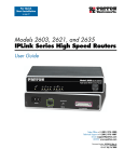
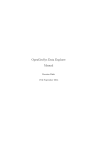
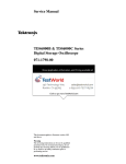
1
User Guide Version 6.0 Volume III: POST-PROCESSING 'Resolution of partial differential equations is more about art than science'. Apocryphal quotation from Numerical Recipes in Fortran “2+2=4 except for large values of 2” Anonymous “42” Douglas Adams edited by: Margarita Bambach and Georg J. Schmitz Contents Contents .................................................................................................................. 3 1 How to use this manual ...................................................................................... 1 2 Introduction ......................................................................................................... 2 Post-Processing ..................................................................................................... 4 3.1. Introduction to MICRESS® Post-Processing .......................................................4 output file types ................................................................................................. 5 3.1.1. mcr files ................................................................................................ 5 3.1.2. ASCII/txt files ........................................................................................ 8 3.1.3. vtk files ............................................................................................... 10 3.2. Overview of post-processing tools for MICRESS® results ................................. 11 4 DP_MICRESS ................................................................................................ 12 4.1. Installing DP_MICRESS ......................................................................................12 4.2. Using DP_MICRESS ...........................................................................................13 4.2.1. The graphics window .......................................................................... 14 4.2.2. The operating window ........................................................................ 15 4.2.3. The control panel ................................................................................ 16 4.2.4. Navigating the results ......................................................................... 17 4.2.5. Setting scales ..................................................................................... 18 4.2.6. Colour scales...................................................................................... 19 5 4.2.7. Run animations .................................................................................. 21 4.2.8. Setting view options ........................................................................... 22 4.2.9. Selecting displayed items ................................................................... 24 4.2.10. Using symmetry operations ............................................................ 25 4.2.11. Handling isolines ............................................................................ 26 4.2.12. Visualizing 3D results with DP_MICRESS ..................................... 28 4.2.13. Displaying vector fields................................................................... 29 4.2.14. Generating output .......................................................................... 30 4.2.15. Virtual EDX ..................................................................................... 32 4.2.16. Virtual EDX output .......................................................................... 34 4.2.17. Data information ............................................................................. 36 4.2.18. Miscellanea .................................................................................... 38 ParaView ....................................................................................................... 39 5.1. Installing and running ParaView ..........................................................................39 5.2. Using Paraview ......................................................................................................41 5.1.1. Display surface or volume .................................................................. 41 5.1.2. Rotation/Translation ........................................................................... 42 5.1.3. Colour by different results and attributes ............................................ 43 5.1.4. Run an animation ............................................................................... 44 5.1.5. applying filters/setting thresholds/making sections ............................. 45 6 gnuplot ............................................................................................................... 46 6.1. Installing gnuplot ................................................................................................47 6.2. Plotting data and fitting curves .........................................................................48 6.3. Comparing different data ....................................................................................50 7 Data conversion: *.mcr to *.vtk ......................................................................... 51 8 9 Post-processing Exercises ......................................................................... 53 8.1. Introduction to post-processing exercises with DP_MICRESS.......................53 8.2. Read and handle a single result file for a single time step ..............................53 8.3. Read and handle a single result file for multiple time steps ...........................56 8.4. Read multiple result files ...................................................................................57 Useful Information and FAQs ...................................................................... 60 9.1. Why can I not open a certain 3D output file by DP_MICRESS?.......................60 9.2. How to calculate the *.intf-output ......................................................................61 9.3. How to combine phase boundaries and concentration in DP_MICRESS .......61 9.4. DP_MICRESS does not show any letters or numbers in plots ........................62 9.5. How to save an animation as a direct output in DP_MICRESS? .....................62 10 References ....................................................................................................... 63 11 Index ................................................................................................................. 64 Chapter 1 How to use this manual 1 How to use this manual The “Introduction” shortly presents the capabilities of the software as well as its wide range of applications. It also introduces the recent developments and improvements of MICRESS®. The chapter “Post-Processing” offers an overview of the MICRESS® result files and presents the freeware that can be used for processing, analyzing and visualisation of MICRESS® output. The capabilities of the programs DP_MICRESS, ParaView and gnuplot are discussed in the subsequent chapters. Information is given about how to install these software tools and how to use their graphical interface. The chapters also provide some examples of possible evaluation and visualisation that may be helpful when post-processing MICRESS® results. Some “Post-processing exercises” may be helpful to get better acquainted with the evaluation of MICRESS® results. You may find further useful hints for generating specific output and troubleshooting in “Useful Information and FAQ”. Any suggestions or comments for improvements on the MICRESS® manual and documentation are highly appreciated and welcome. Please send an e-mail to [email protected]. MICRESS® User Guide Volume III: Post-Processing 1/70 Chapter 2 Introduction 2 Introduction The software MICRESS® (MICRostructure Evolution Simulation Software) is developed for time- and space-resolved numerical simulations of solidification, grain growth, recrystallisation or solid state transformations in metallic alloys. MICRESS® covers aspects of phase evolution, solutal and thermal diffusion and elastic stresses/strains in the solid state. It enables the calculation of microstructure formation in time and space by solving the free boundary problem of moving interfaces on the basis of a multiphase field approach. Microstructure evolution is governed essentially by thermodynamic equilibria, diffusion and curvature. In case of multicomponent alloys, the required thermodynamic data can either be provided to MICRESS® in the form of locally linearized phase diagrams, or by direct coupling to thermodynamic data sets via a special TQ interface, developed in collaboration with Thermo-Calc™ AB, Stockholm. MICRESS® is based on the multi-phase-field method which defines a phase-field parameter for each phase being involved. The phase-field parameter describes the fraction of each phase as a continuous function of space and time. Each single grain is mapped to a distinct phase-field parameter and is treated as an individual phase. A set of coupled partial differential equations describes the evolution of the phase-field parameter(s) and of the concentration, temperature, stress and flow fields. The total set of equations is solved explicitly by the finite difference method on a cubic grid. 2D and 3D simulations are possible. The size of the simulation domain, the number of grains, phases and components is restricted mainly by the available memory size and the CPU speed. MICRESS® User Guide Volume III: Post-Processing 2/70 Chapter 2 Introduction MICRESS® handles: 1-, 2- and 3-dimensional calculation domains arbitrary number of components, phases and grains solid-solid and solid-liquid interactions anisotropy of grain boundaries, mobility and energy MICRESS® supports: coupling to thermodynamic database (via the TQ-interface of Thermo-Calc™) In the present MICRESS® Vol.3 “post processing” you will find: an overview of the different MICRESS® result files an overview of the available software for post-processing of MICRESS® result files a short overview of the functions of DP_MICRESS, ParaView and gnuplot examples of possible data post-processing some useful information, troubleshooting and frequently asked questions A description of the phase-field phenomenology and theoretical background can be found in MICRESS Vol. 0: “MICRESS phenomenology” along with a review type summary of different MICRESS applications. MICRESS Vol. I: “Installing MICRESS” provides information about the installation of the software and explains how to use the software with the help of a simple example. MICRESS Vol. II: “Running MICRESS” offers an overview of the input file structure, as well as theoretical and practical information on metallurgical processes, numerical modelling using the phase-field model and troubleshooting when starting a simulation. It provides useful hints on how to build the input file according to the process to be simulated. Eventually, MICRESS Vol. IV: “MICRESS Examples” contains a collection of examples of simulations performed on various topics. MICRESS® User Guide Volume III: Post-Processing 3/70 Chapter 4 DP_MICRESS Post-Processing 3.1. Introduction to MICRESS® Post-Processing Before starting post-processing, make sure that the files to be analysed are the most recent ones you created. It is often useful to check whether MICRESS® has really started creating the output immediately after starting the simulation. For this purpose it is often wise to compare the computer time and the time of file creation/update in the results directory. Once you have verified the right output files, you should decide about the best of postprocessing the individual files according to their contents. The different output file types are shortly highlighted in the following. MICRESS® User Guide Volume III: Post-Processing 4/70 Chapter 4 DP_MICRESS output file types MICRESS® generates the following categories of result files: files containing field values, the “.mcr” files ASCII “.txt” files containing statistical information optional: “vtk” files (especially for 3 D results) 3.1.1. mcr files Three different classes of MICRESS result files (“.mcr”) can be distinguished: special .mcr files standard .mcr files 1d_extension .mcr files The meaning and content of these files is described in the following tables: Special “.mcr” output files: output *geoF.mcr Description a geometry file being necessary for any post-processing. It stores information concerning the geometry of the simulation domain e.g. grid size, cell dimensions, etc. This is file is used by any post-processing program for the visualisation of results. *rest.mcr a restart file that allows to restart/continue a simulation. MICRESS® User Guide Volume III: Post-Processing 5/70 Chapter 4 DP_MICRESS Results for the individual field variables (2D, 3D) for all output time steps in standard “.mcr” files: output Description *.concN.mcr gives information about the concentration of the alloying element N *.cPhaN.mcr similar to *.concN, except for the interface regions, where the concentration in a given phase is written out and not the mixture concentration *.dGsp.mcr used in stress-coupled simulations; it shows the stress contribution to the driving force *.diff.mcr shows the data provided by Thermo-Calc™ via its TQ interface for the diffusion coefficients *.driv.mcr gives the driving force for the growth of a grain with a higher number into a lower one *.frac.mcr yields the fraction of solid *.fracN.mcr shows the fraction of the phase N *.geoF.mcr stores information concerning the geometry (i.e.: grid size, cell dimension) *.hStr .mcr provides information about the hydrostatic stress, when the stress coupling is activated *.intf .mcr provides data fro tracking the interface *.korn.mcr a graphical output for the grain field, containing the numbers assigned to grains in a consecutive manner during their definition in the initial grain structure or their nucleation during runtime *.krum.mcr gives information about the interface curvature *.millx.mcr also *.milly and *.millz lists the respective Miller indices *.mueS.mcr gives information about the local interface mobility *.orie.mcr stores the 2D-grain orientation MICRESS® User Guide Volume III: Post-Processing 6/70 Chapter 4 DP_MICRESS *.phas.mcr provides information on the phases in the system *.rest.mcr contains data necessary to restart a simulation; this binary file is for internal use by MICRESS® and cannot be post-processed *.rex .mcr lists the stored energy *.sxxCV.mcr also *.sxyCV, *.sxzCV, *.syyCV, *.syzCV and *.szzCV components of the stress tensor, xxCV, (yyCV), zzCV are the diagonal elements in the 2D (3D) case, sxyCV, sxzCV, syzCV are off-diagonal terms (torsion), respectively. The output is available when stress coupling is activated. *.temp.mcr For the temperature in Kelvin, when temperature coupling is activated. It can be also used for plotting temperature-distance profiles. *.uxCV.mcr also *.uyCV and *.uzCV. They record the normal displacements when the stress coupling is activated. *.vel.mcr gives out the interface velocity *.vxCV.mcr also *.vyCV, *.vzCV, *.syyCV, *.syzCV and *.szzCV: components of the stress tensor; xxCV, (yyCV), zzCV are the diagonal elements in the 2D (3D) case, sxyCV, sxzCV, syzCV are off-diagonal terms (torsion), respectively. This is true if the stress coupling is activated. *.vM.mcr gives out the von Mises stress when stress coupling is activated. Results for individual field variables calculated in extended 1D fields (1DExt): output Description *1DExt_conc1.mcr shows the concentration of alloy element 1 as specified in the MICRESS driving file, when a 1D external field has been used in the simulation *1DExt_conc2.mcr shows the concentration of alloy element 2 as specified in the MICRESS driving file, when a 1D external field has been used in the simulation *1DTemp_Temp.mcr gives the temperature when a 1D temperature field is used *1DTemp_enth.mcr shows the enthalpy when a 1D temperature field is used MICRESS® User Guide Volume III: Post-Processing 7/70 Chapter 4 DP_MICRESS 3.1.2. ASCII/txt files Two different classes of MICRESS ASCII result files (“.txt”) can be distinguished: special .txt files standard .txt files The meaning and content of these files is described in the following tables: Special “.txt” output files: output *in. txt *log.txt Description the input file corresponds to the driving file as understood by MICRESS®. gives information about the input data, initial relinearisation output at initialisation or before the first nucleation, CPU time and intermediate output at defined time steps “.txt” files containing dedicated data: output Description for the average and extrema of concentration in each phase, *.TabC.txt when the concentration coupling is activated *.TabD.txt gives the diffusion coefficients at the corresponding “tab_log” times, when the concentration coupling is activated MICRESS® User Guide Volume III: Post-Processing 8/70 Chapter 4 DP_MICRESS *.dTLat.txt used for intermediate data relative to the release of latent heat *.TabF.txt for the average fraction of each phase in the whole domain, when the concentration coupling is activated *.TabGD.txt contains information about the grain status, i.e. whether a grain increases in dimensions *.TabK.txt contains the number of grains. This file is updated by default each time a grain is set or disappears. *.TabL.txt an ASCII-monitoring output generated at user-defined intervals to check the simulation progress; it gives information on the temperature gradient and some additional information depending on the type of coupling activated. *.TabLin.txt it gives the temperature at defined time intervals for the temperature at the bottom and at the connecting points when linear flow trend used *.TabN.txt stores data relevant for making “Von Neumann – Mullins plots” *.TabP.txt sums up the simulation time, the CPU time, the diffusion, the seed, the enthalpy, the stress and the temperature times *.TabR.txt provides information on the recrystallized fraction *.TabO.txt gives orientation information *.TabT.txt reports information concerning the setting of the (automatic) timestep, when automatic time-stepping has been selected *TabTQ.txt shows the temperature change with progressing simulation time and the corresponding CPU time *TQ.txt a Windows-specific data file which stores the output of ThermoCalc´s interface making it more convenient to exploit the origin of TQ errors. It is always created under Windows when ThermoCalc™ -coupling is activated MICRESS® User Guide Volume III: Post-Processing 9/70 Chapter 4 DP_MICRESS 3.1.3. vtk files Especially for 3D simulations, e.g. fig. 3.2, there is an option to save simulated data in a special format called “vtk”. This format allows 3D visualisation of the results in freeware software tools like e.g. paraview (www.paraview.org; see chapter 5). This output option can be switched on in the driving file for the simulation. As a consequence, “vtk” files are written out instead of “mcr” files. The major difference between these two output formats is, that a “mcr” file contains the results for one field variable for all time steps, while each “vtk” file comprises all field variables for only one time step. A conversion of “mcr” files to “vtk” files is possible using the DP_MICRESS tool (see chapter 7). Fig 3.2 3 D Simulation of a an array of Mg dendrites with the results being saved and displayed in the vtk format MICRESS® User Guide Volume III: Post-Processing 10/70 Chapter 4 DP_MICRESS 3.2. Overview of post-processing tools for MICRESS® results Currently available freeware frequently used for post-processing different MICRESS® result files comprises: DP_MICRESS. This is a 2D (partially 3D) evaluation tool, the graphical user interface to Display MICRESS. This tool is provided along with your MICRESS® installation CD. ParaView. This is a freely available 3D post-processor from ParaView (www.paraview.org) gnuplot. This command-line driven plotting utility can be used for post-processing of text and ASCII files. It can be downloaded from www.gnuplot.info. The ASCII and txt result files can be also post-processed with any type of ASCII post-processing, e.g. MS Editor, Excel, etc. software 2D 3D gnuplot ParaView DP_MICRESS text ASCII ® Fig 3.3 Categorisation of the currently available freeware for post-processing of MICRESS results These tools and their basic operation will be shortly introduced in the following chapters. MICRESS® User Guide Volume III: Post-Processing 11/70 Chapter 4 DP_MICRESS 4 DP_MICRESS 4.1. Installing DP_MICRESS DP_MICRESS is the graphical user interface to Display MICRESS. It is a post-processing tool with a wide span of possibilities, ranging from basic display and image output, to advanced features such as zooming, multiple display, build-in symmetry options, animations and virtual EDX analysis. It can handle several files simultaneously. DP_MICRESS is preferentially used for reading and post-processing 2D and 3D MICRESS® output files It reads result files in binary (single and double precision, native or not) and ASCII-format, both compressed and not-compressed. Moreover, it performs conversions between these formats. This post-processing downloaded from the tool can download be freely area Figure 4.1. The initial window of Display MICRESS at www.micress.de. MICRESS® User Guide Volume III: Post-Processing 12/70 Chapter 4 DP_MICRESS Command-Line C:\ cd Desktop\Results_Delta_Gamma C:\ DP_MICRESS Delta_Gamma_intf.mcr Display MICRESS can also be called from a shell, providing the name of the result file(s) to be displayed. It can be called by entering e.g. DP_MICRESS Delta_Gamma_intf.mcr in the command line. If no argument is provided, a summary of command line-options is returned. Alternatively, under Windows, the program can be activated by double-clicking the DP_MICRESS icon. To select a result file to be displayed, go to Display → Select (see Figure 4.1.). A result file can be also simply “dragged and dropped” to the DP_MICRESS icon. DP_MICRESS always initially shows the result for the first time step. Use the buttons “next” and “last” to view the results for the next time steps. The program does not allow switching between files, i.e. it has to be restarted to display another result file. 4.2. Using DP_MICRESS DP_MICRESS uses a graphics window, an operating window and a control panel to visualize and process MICRESS® results. These windows/panels are explained in detail in the following chapters. MICRESS® User Guide Volume III: Post-Processing 13/70 Chapter 4 DP_MICRESS 4.2.1. The graphics window The output files are displayed in the graphics window, Figure 4.2. Details about how to alter the appearance of this window will be given in the respective chapters below. Figure 4.2. Visualization of the example Delta_gamma_intf.mcr: interface output for the first (middle) and the last (right) time step. The actual time step is shown in the upper left corner of each figure. The lower left corner gives information about the displayed field/type of result. Information about the domain size is given in the insert. The domain size in micrometers is given by the number of cells in x, y and z directions (see e.g. Fig. 4.2, insert) multiplied by a scaling factor e.g. 1 m/cell, which is defined in the driving file. To obtain the real dimensions of the domain a scale bar option can be used. MICRESS® User Guide Volume III: Post-Processing 14/70 Chapter 4 DP_MICRESS 4.2.2. The operating window The operating window of DP_MICRESS (Figure 4.3.) pops up automatically and helps to process and visualise the selected output file. It provides useful hints on selected functionalities. Following the instructions given in this operating window will often facilitate work. Also, some special results are displayed here. Examples are e.g. the distance between two points, the value of an angle, the angle between a line and its horizontal, etc. Points, distances and angles to be directly measured by the are user defined on the displayed graph. Keep an eye on the output in the operating window while processing your results. You can switch among different options using the control panel. The individual functions of DP_MICRESS the control panel will be detailed in the next section Figure 4.3. The operating window of DP_MICRESS MICRESS® User Guide Volume III: Post-Processing 15/70 Chapter 4 DP_MICRESS 4.2.3. The control panel The graphical visualisation of the result output file can be navigated via the control panel (see Figure 4.4). Here, e.g. the colour scale may be adjusted, an animation may be created or a virtual EDX may be displayed. The options to navigate, visualize, analyze, animate and save the results will be explained briefly in the next sections. General Hints: If you click on the dashed line of a sub-menu (see red rectangle in Fig.4.4.), the sub-menu will open and remain available to facilitate work. Most of the functions/actions can be “undone” by reselecting the corresponding option. Figure 4.4. The DP_MICRESS control panel: jump MICRESS® User Guide Volume III: Post-Processing 16/70 Chapter 4 DP_MICRESS 4.2.4. Navigating the results Navigating the results means finding and selecting the time step of the result being of interest. There are several options: next: displays the next time step in the graphics window previous: displays previous time steps last: displays the last time step first: displays the first time step The option jump has the following features (see Fig 4.4): ◦ jump to time-step specified by its number: allows to jump to a specific output number (not corresponding to the „time“) ◦ report output time(s): the output numbers for the time steps is specified in the operating window ◦ pick time-step to jump to with a graphical interface: the user chooses manually the time steps for which results shall be displayed dissociated: allows navigating/viewing different result types independently at different time steps. Each result type then must be navigated separately. Here, the options next, previous, last, first, jump to time-step specified by its number, report output time(s) and pick time-step to jump to with a graphical interface are also available. MICRESS® User Guide Volume III: Post-Processing 17/70 Chapter 4 DP_MICRESS 4.2.5. Setting scales The option scale of the control panel offers the following features, Figure 4.5: set min./max: manual setting of the scales (min-max) for the individual results. The minimal and the maximal values are displayed in the graphics window. set range: manual setting of the scales (a predefined range) for the individual results. A median value and a range are displayed in the graphics window. min./max. from display: automatic setting of the scales for the individual results to the minimum/maximum of the actually displayed result/time step. A median value and a range are displayed in the graphics window. global min./max.: automatic setting of the scales to the minimum/maximum occurring in all time steps for the individual results (similar to “replot”). The values are displayed in the Figure 4.5. The DP_MICRESS control panel: scale graphics window re-read file for global min./max.: same as before, but the results are re-read to ensure evaluation of the full data set. Here, no values are displayed in the graphics window. MICRESS® User Guide Volume III: Post-Processing 18/70 Chapter 4 DP_MICRESS 4.2.6. Colour scales The option colour scale, fig. 4.6, provides following features: loop through colour scales: displays the available colour scales loop backwards through colour scales: same as above, but displays the scales in a reverse order. select colour scale: allows selection of a colour scale e.g. after viewing them in one of the „loop“ commands fiddle with brightness & contrast: changes brightness and/or contrast using the mouse. Click on the graph to activate the selected values. reset brightness & contrast: resets to the previous value inverse colour scale: inverts the colours in the colour scale (the colour for the minimum value becomes the colour for the maximum one and vice versa) Figure 4.6. The DP_MICRESS control panel: colour scale cut off min. and max.: cuts off minima and maxima and replaces respective regions by black and white MICRESS® User Guide Volume III: Post-Processing 19/70 Chapter 4 DP_MICRESS stepwise colour scale: selects colour scale to colour regions being specified. The colours of the scale change continuously set number of steps: allows to define number of colour regions, e.g. if you enter 3, you will have only three colours in your scale. Thus, each of the colours will cover a wider range of values. automatic number of steps: selects a suitable number of colour regions automatically random colour scale: define a random colour scale (only for LINUX) set seed random colour scale: initialize random generator for random colour scale (only for LINUX) Figure 4.7. Examples of different colour scales available by DP_MICRESS. The result file is Delta_Gamma_phas.mcr at its last time step. MICRESS® User Guide Volume III: Post-Processing 20/70 Chapter 4 DP_MICRESS 4.2.7. Run animations The option animation, fig. 4.8, has the following features: run animation: animates the entire simulation from the beginning to its end with a time per section and number of repetitions as defined under animation settings animate to the end: animates the simulation starting from the actual time step up to its end animation settings: allows to set animation parameters (time per section and number of repetitions). Default settings are 2 repetitive runs and a time per section of 0.75 seconds. To alter these values, click on the displayed values and enter new ones. Figure 4.8. The DP_MICRESS control panel: animation MICRESS® User Guide Volume III: Post-Processing 21/70 Chapter 4 DP_MICRESS 4.2.8. Setting view options The option view, fig 4.9, has the features set nb. of panels: allows for shuffling of several results into columns and rows. The number of panels describes the amount of plots allowed per line and row. If you enter “3” for horizontal and “1” for vertical and use a “row major order”, results in a configuration like fig. 4.10. Toggle between “previous” and “next” to choose which two (consecutive) plots shall be displayed freeze panel: this function is disabled replot: replots the display e.g. following a parameter change auto-replot on/off: automatic replotting resize and auto-resize on/off: automatic resizing Figure 4.9. The DP_MICRESS control panel: view annotations: you can choose which annotations to display or whether not to display annotations at all by using this button. There are four different modes of displaying annotations available, which can be addressed by multiple clicking this option. orientation l/r <-> b/t: the annotation position is switched from left/right to bottom/top and vice versa MICRESS® User Guide Volume III: Post-Processing 22/70 Chapter 4 DP_MICRESS increase thickness of colour scale: four different sizes for the annotations can be selected by repeated activation of this button. If you select view → annotations once, you would see your plot together with comments and a colour scale. If you select it twice, the graph will be displayed with a colour scale only. If selected three times, the plot will be displayed with comments, but without a colour scale. Selecting the command four times displays neither comments, nor colour scale. display temperature at the bottom: displays the temperature at the bottom of the simulation domain Fig 4. 10 Set number of panels When opening more than two files, a rearrangement of the different results makes them better readable. Use this function to shift from the default setting (left) to an aligned configuration (right) MICRESS® User Guide Volume III: Post-Processing 23/70 Chapter 4 DP_MICRESS 4.2.9. Selecting displayed items The menu display, fig. 4.11, offers the following features, many of them being self explanatory: display length scale: inserts a length scale into the lower right corner of the display set length to be displayed: defines the length of the scale flip length scale (vertical/horizontal): selects orientation of the length scale zoom in: allows for a closer look at the details zoom out: goes back to the larger view zoom back: (revert to previous zoom settings) toggle on/off display of raster special symmetry operations: (see separate chapter 4.2.10) display grid set nb. of gridlines display difference of two results logarithmic display of results Figure 4.11. The DP_MICRESS control panel: Display absolute value of results toggle on/off display of raster MICRESS® User Guide Volume III: Post-Processing 24/70 Chapter 4 DP_MICRESS 4.2.10. Using symmetry operations switch symmetry: toggle through symmetry options below three-folded symmetry: selects a 3-fold symmetry four folded symmetry: selects a 4-fold symmetry nine-folded symmetry: selects a 9-fold symmetry symmetry type: select symmetry type (translational symmetry or mirror symmetry) see Figure 4.13 for some examples of symmetry operations Figure 4.12. The DP_MICRESS control panel: view Figure 4.13. Different symmetries activated in DP_MICRESS. The result file shown here is Delta_Gamma_phas.mcr at t=50 s MICRESS® User Guide Volume III: Post-Processing 25/70 Chapter 4 DP_MICRESS 4.2.11. Handling isolines The option isolines, fig. 4.14 has the features, display isolines: (see fig. 4.15.) shows/hides pre-defined isolines label isolines: creates labels for the individual isolines auto isolines: activates preset isolines (see fig. 4.15.) add “n” auto-isolines: adds a number of „n“ own isolines remove an isoline: removes a selected isoline remove all isolines: removes all isolines display contours: shows only the contours (see Figure 4.15) print isolines values: returns values of isolines in the operating window bicolour isolines: changes the colour of the isolines (black ↔ white) write contour output: writes a .txt-file comprising the coordinates of a preselected isoline for the current time step write contour outputs: writes a .txt-file comprising the coordinates of a preselected isoline for all time steps Figure 4.14. The DP_MICRESS panel: isolines MICRESS® User Guide Volume III: Post-Processing control 26/70 Chapter 4 DP_MICRESS a) mapping of carbon b) with isolines at c = 1.02, (conc1) without isolines 1.01 and 1.005 at% c) isoline contours only Fig 4.15. Different options for displaying concentration isolines (here: Delta-Gamma results for carbon at t=30 s) MICRESS® User Guide Volume III: Post-Processing 27/70 Chapter 4 DP_MICRESS 4.2.12. Visualizing 3D results with DP_MICRESS Actually, DP_MICRESS is not a full 3D viewer. For 3D post-processing thus the ParaView tool (see chapter 5) is recommended. DP_MICRESS allows creating sections parallel to the coordinate system. These sections can then be analysed with the tools known for 2D analysis. The navigation and selection of a sectional plane proceeds as follows, fig. 4.16: xy cutting plane, xz cutting plane and yz cutting plane allow to select the plane to be displayed (default XZ-plane) cutting plane up/down : increases/decreases the position of the cutting plane (the Ycoordinate by default) set cutting plane coordinate: sets the position of the cutting plane (the Y-coordinate by default) Fig 4.16 The 3D-menue MICRESS® User Guide Volume III: Post-Processing 28/70 Chapter 4 DP_MICRESS 4.2.13. Displaying vector fields Displaying vector fields needs at least three different result files to be displayed. One of these result files provides the “background” for displaying the vectors, while the two (three) further result files are the different components of the vector in 2D (resp. 3D), Figure 4.17. Currently only the MICRESS elastic module provides a vector valued output. In future also the MICRESS flow module will make use of vector field displays. toggle on and off vector display (2D) toggle on and off vector display (3D): same as above, but for 3D. modify vector field display settings display vector field scale (together with bicolour vectors) Fig 4.17 Generating vector display for the example of a flow field around a dendrite in 2D. Based on 3 result files (one for the background and two for the two components of the vector (left) a vector field can be displayed using the vector filed option (right) MICRESS® User Guide Volume III: Post-Processing 29/70 Chapter 4 DP_MICRESS 4.2.14. Generating output Using the option output, the following outputs can be generated (see figure 4.18) image from current time-step: creates an image of the current time step. You should define the path at which the file shall be saved. image from all time steps: creates a series of images for all time steps. The images are written in the folder where the ® corresponding MICRESS are to be found. write larger images: creates larger size images with toggle on/off write high resolution images: creates high resolution images with toggle on/off ASCII output from current: creates ASCII output for current time step at a defined path. ASCII output from all time steps: creates ASCII output for all time steps at the already specified path. Raster ASCII output from current: creates Figure 4.18 The DP_MICRESS control panel: output ASCII output for current time step at a defined path. You should specify the desired grid spacing in m. Raster ASCII output for all time-steps: creates ASCII output for all time steps at a defined path. You should specify the desired grid spacing in m. colour scale: saves selected colour scales as images. MICRESS® User Guide Volume III: Post-Processing 30/70 Chapter 4 DP_MICRESS output numbering: creates a numbered ordering of the output with toggle on/off. This is useful where filenames become too long otherwise. image driver: gif/postscript: toggle data format for image files gif/ps. accept default naming …or do not! ..toggle for selecting own nomenclature. Hints: In order to increase the output readability, try the following: ▪ increase the thickness of the colour scale ▪ use black and white plots instead of colourful ones ▪ use white background to save ink ▪ use axes labelling MICRESS® User Guide Volume III: Post-Processing 31/70 Chapter 4 DP_MICRESS 4.2.15. Virtual EDX The option virtual EDX offers the following features (Figure 4.19. and Figure 4.20): Display scan: draw a line using the mouse. A scan will be defined along the line. Follow the instructions in the operating window. The results are displayed in the graphics window (see Figure 4.18.). Select scan e.g. phas. Display scans for all time steps: displays scans for a predefined line (by display scan or linescan x/y for all time steps). Keep an eye on the operating window for instructions. Linescan X: enter the desired coordinates of the line along which the scan shall be displayed. Press the ENTER key. The graphics window shows the line that corresponds to the defined coordinates. After that, the scan is displayed. Linescan Y: similar to the option Linescan X but along the Y- Axis. Figure 4.19. The DP_MICRESS control panel: virtual EDX Replot scan line: the scan line can be thus replotted Rescan previously selected line: the function is self- explanatory. Normalise scans: Allows for normalising the diagrams to an integral value of 1. Follow the command line for instruction. MICRESS® User Guide Volume III: Post-Processing 32/70 Chapter 4 DP_MICRESS Front tracking: allows for tracking the evolution of a value in space and time. Give a value to be tracked and press the ENTER key. The corresponding scan is displayed in the graphics window. Scan point: tracks the value at a scan point along time. Important: Virtual EDX of different solutions may be difficult to compare. For comparison, consider carefully which solutions to plot. Normalising the solutions may be helpful. C1 field value C2 C1 liquid solid µm 50 100 150 Figure 4.20. The two dimensional concentration output for the last time step of Delta_Gamma (top,left) and a scan (green) above the dendrite tip in the liquid state results in a virtual EDX for both elements (top,right) being sketched schematic (bottom). MICRESS® User Guide Volume III: Post-Processing 33/70 Chapter 4 DP_MICRESS 4.2.16. Virtual EDX output Using the option virtual EDX output, fig. 4.21, the different types of output can be generated. However it is important to actually create data first with virtual EDX before choosing the create output-option. virtual edx scan position for current time-step: generates an image including the scan line for current time step at a path specified by the user. virtual edx scan position for all time-steps: generates images including the scan line for all time steps at the path where the corresponding MICRESS® output files are to be found. virtual edx curves output from current time-step: generates a graphics output of the field values along the scan line for the current time step at a path specified by the user. virtual edx curves output for all time-steps: generates graphics output of the field values along the scan line for all time steps at the path where Figure 4.21. The DP_MICRESS the control panel: virtual EDX output files are to be found. corresponding MICRESS® output virtual edx curves output for selected time-steps: generates graphics output of the field values along the scan line for selected time steps at a path specified by the user. Front tacking text output: lists all positions, where a specified field value is present. The output is generated for all times at a path specified by the user. MICRESS® User Guide Volume III: Post-Processing 34/70 Chapter 4 DP_MICRESS virtual edx text outputs for all time-steps: generates an ASCII type output of the field values along the scan line for the all time steps at the path where the corresponding MICRESS® output files are to be found. virtual edx text output from current time step: generates an ASCII type output of the field values along the scan line for the current time step at a path specified by the user. virtual edx scan position for current time-step: generates an image including the scan line for current time step at a path specified by the user. virtual edx scan position for all time-steps: generates images including the scan line for all time steps at the path where the corresponding MICRESS® output files are to be found. virtual edx curves output from current time-step: generates a graphics output of the field values along the scan line for the current time step at a path specified by the user. virtual edx curves output for all time-steps: generates graphics output of the field values along the scan line for all time steps at the path where the corresponding MICRESS® output files are to be found. virtual edx curves output for selected time-steps: generates graphics output of the field values along the scan line for selected time steps at a path specified by the user. Front tacking text output: lists all positions, where a specified field value is present. The output is generated for all times at a path specified by the user. scan point text output: lists the field values at a defined scan point over time as a text output at a path specified by the user. scan point position output: saves pictures with an indicated scan point position at a path specified by the user. scan point curve output: saves the field values at a defined scan point over time as a diagram. The path where the graph is saved is defined by the user. MICRESS® User Guide Volume III: Post-Processing 35/70 Chapter 4 DP_MICRESS 4.2.17. Data information The option data information offers the following features, figures 4.22. and 4.23 distance between two points: measures the distance by drawing a line with the mouse (hold the left mouse button). The line length is shown in the operating window. measure angle: measures angles by drawing two lines with the mouse (select the left button of the mouse twice). The angle is given in both degrees and radians in the operating window. measure angle with horizontal: measures the angle to a horizontal line by drawing a line with the mouse. The angle is given in both degrees and radians in the operating window. measure angle with vertical: measures angles to a vertical line by drawing one line with the mouse. The angle is given in both degrees and radians in the operating window. extrema and average from display: defines the average and the extrema of the current time step. The results are displayed in the operating window. coordinates (field value) of a point: defines a Figure 4.22. The DP_MICRESS control point to be investigated by a mouseclick. Also, panel: Data Information returns the number of the cell, i.e. the „cell pointer“. The results are displayed in the operating window. MICRESS® User Guide Volume III: Post-Processing 36/70 Chapter 4 DP_MICRESS compare all outputs: as compare results but for all time steps pinpoint cell pointer: returns field values/coordinates of a specific numerical cell. The results are displayed in the operating window compare results: offers a comparison of two results for a given time step. The input value defines a tolerance within which both results are considered to be identical. The operating window returns the statement that the compared values are either identical or different. version information: returns the actual version of DP_MICRESS in the operating window print information about geometry: returns information about the geometry, the actual zoom status and the symmetry in the operating window Figure 4.23 The data information feature: determination of the field values and coordinates of a point (left), the vertical distance (middle) and measuring an angle (right). The data being determined are displayed in the operating window. The result file shown is Delta_Gamma_conc.mcr MICRESS® User Guide Volume III: Post-Processing 37/70 Chapter 4 DP_MICRESS 4.2.18. Miscellanea The options miscellanea and exit are characterised by the following features: suspend GUI: allows to show all options of key-combinations. Follow the command line for instructions and information. remove output: removes a selected time step from the output. Important: be careful, the present result files will be overwritten! about: provides information on Display_MICRESS (current version, acknowledgements, website for further information etc.) exit: terminates the program MICRESS® User Guide Volume III: Post-Processing 38/70 Chapter 5 ParaView 5 ParaView 5.1. Installing and running ParaView The freeware ParaView is especially useful for post-processing of 3D MICRESS output data (Figure 5.1.). The software can be downloaded for free from www.paraview.org. ParaView requires a vtk-format of the files to be read. To exploit how to create a vtk-file from existing MICRESS results, please refer to chapter 7 of this handbook on “Data conversion”. There are also options to directly specify/create vtk output from MICRESS simulations. Please note, that within this manual only a very basic introduction can be given, as there are many, many options for the use of ParaView. To open an existing vtk-file in ParaView, run the program. In the main menu bar, go to File → Open. Choose the file to be opened. It will usually appear as “filename_.vtk”. The selected file appears in the tree of built-in objects in the left side of the ParaView window. Click on “apply” under object inspector → Properties (the sub window below the built-in objects tree). Then, the calculation domain (similar to Figure 5.1. of your simulation will appear in the window right. MICRESS® User Guide Volume III: Post-Processing 39/70 Chapter 5 ParaView Figure 5.1. A MICRESS 3D result output displayed using ParaView Figure 5.2. Opening a vtk-file in ParaView (left) and the simulation domain (right) MICRESS® User Guide Volume III: Post-Processing 40/70 Chapter 5 ParaView 5.2. Using Paraview 5.1.1. Display surface or volume Once having loaded the result file, use the button shown in fig. 5.3 (marked in red) to switch among „outline“, „surface“, „volume“ and „slice“. Observe how the simulation domain changes its appearance. Figure 5.3. The ParaView main menu bar: the Volume feature MICRESS® User Guide Volume III: Post-Processing 41/70 Chapter 5 ParaView 5.1.2. Rotation/Translation Pressing the left mouse button and moving the mouse at the same tile leads to free rotation. Pressing the right mouse button with moving the mouse simultaneously zooms in and out. A rotation around an axis is possible via pressing the „shift“ and the „left“ mouse button with simultaneously moving the mouse. For translation, press the „shift“ button and the „right“ mouse one and move the mouse. MICRESS® User Guide Volume III: Post-Processing 42/70 Chapter 5 ParaView 5.1.3. Colour by different results and attributes Use the button coloured in red (Figure 5.4.) to switch between different output results. The simulation domain will be coloured according to the output file selected in the menu bar (see figure Fehler! Verweisquelle konnte nicht gefunden werden.5.5). Figure 5.4. The ParaView main menu bar: the attribute feature Figure 5.5. Colouring the simulation domain according to the different attributes of the output file MICRESS® User Guide Volume III: Post-Processing 43/70 Chapter 5 ParaView 5.1.4. Run an animation You can run an animation using the output for a given attribute for all time steps. For that purpose, use the animation bar in the main menu (Figure 5.6). You can easily switch between previous and next time steps, go directly to the very first/last time step or perform different loops of visualisation. Figure 5.6. The ParaView animation bar MICRESS® User Guide Volume III: Post-Processing 44/70 Chapter 5 ParaView 5.1.5. applying filters/setting thresholds/making sections The clip filter cuts away a portion of the input data set using an implicit plane. It returns unstructured grid data on output. Some of the possible options here are a slice filter, a contour filter, a clip filter and others. With their help, one can easily generate different sections through the calculation domain. Figure 5.7. The ParaView bar for creating clips and thresholds More detailed information about that and all other features of ParaView can be found in the ParaView user's manual. Further information is available at www.paraview.org MICRESS® User Guide Volume III: Post-Processing 45/70 Chapter 6 gnuplot 6 gnuplot gnuplot is a command-line driven interactive function plotting utility for both Windows and Linux platforms. The software is distributed freely and can be downloaded from the internet along with tutorials and user-manuals. Gnuplot handles both curves (2D) and surfaces (3D). Surfaces can be plotted as a mesh fitting the specified function, floating in the 3D coordinate space, or as a contour plot in the X-Y plane. For 2D plots, there are also many plot styles including lines, points, boxes, heat maps, stacked histograms and contoured projections of 3D data. The interface includes command-line editing and history in most platforms. Scope of this chapter is only giving a basic introduction to gnuplot using some MICRESS results as examples. For detailed information the reader is referred to the gnuplot manuals. MICRESS® User Guide Volume III: Post-Processing 46/70 Chapter 6 gnuplot 6.1. Installing gnuplot Figure 6.1. The gnuplot command line after installing gnuplot In order to install gnuplot, first download the installation package from the World Wide Web and then unzip it into an appropriate directory. After having read the “Readme” files and installation instructions, you can run the wgnuplot.exe, Figure 6.1. Using the command-line, you can proceed to visualize and post-process MICRESS® output files. MICRESS® User Guide Volume III: Post-Processing 47/70 Chapter 6 gnuplot 6.2. Plotting data and fitting curves The possibilities of plotting MICRESS® data and fitting curves will be explained with the help of the “Grain Growth” example. This example is stored in the MICRESS® installation directory. Let's consider that you would like to plot the average grain radius over time. This information can be found in the Grain_Growth_.TabK -file (see Figure 6.3.) in the “Grain Growth” result directory. The details for this procedure are explained in fig. 6.2: Fig 6.2 Command-line input for plotting data and fitting curves First specify the path of the respective result file. Then label the axes of the desired plot. If you do not wish to have a legend, use the command “set nokey”. Since this is a 2D plot, only labels for the X and the Y axis are necessary. This is done with the commands set xlabel and set ylabel, resp. The time t for microstructure evolution will be plotted along the X-axis and the grain radius in micrometers will be plotted along the Y-axis. The columns of the data to be plotted are specified by typing e.g. “plot "Grain_Growth_TabK.txt" u 1:2 w l lw 2” where “u 1:2” indicates, that column 2 of the table (see fig 6.2) shall be plotted over column 1 by using a line (w l “with line”) and the line width (lw) shall be 2. MICRESS® User Guide Volume III: Post-Processing gnuplot Command-Line gnuplot> cd 'C:\Desktop\Results_Grain_Growth gnuplot> set nokey gnuplot> set xlabel "t" gnuplot> set ylabel "R/µm" gnuplot> plot "Grain_Growth_TabK.txt" u 1:2 w l lw 2 …. gnuplot> f(x) = R0 + k*x**m gnuplot> R0=1 gnuplot> k=1 gnuplot> m=1 gnuplot> fit f(x) "Grain_Growth_TabK.txt" u 1:2 via R0,k,m gnuplot> replot f(x) w lines gnuplot> print "R0:", R0, "µm" gnuplot> print "k:", k gnuplot> print "m:", m gnuplot> pause -1 48/70 Chapter 6 gnuplot Figure 6.3. The Grain_Growth_TabK.txt-output file: the average radius (column 2) is plotted over the simulation time (column 1) As soon as the last command is entered the plot shown in Fig 6.4 will appear. If you wish to fit the curve e.g. by a least squares fit, specify an analytical function describing the curve. A function of the form f(x) = R0 + k*x**m has been used as an example here (fig 6.2, second part of the gnuplot commands). Figure 6.4. A plot of the grain radius over time Figure 6.5. The original data (red) and the fitted curve (green) Initial values for the parameters R0, k and m have to be specified which will be used as initial guesses during the fitting procedure. Type in “fit f(x) "Grain_Growth_TabK.txt" u 1:2 via R0,k,m” to start the fitting procedure. After the optimal fit has been found, the number of MICRESS® User Guide Volume III: Post-Processing 49/70 Chapter 6 gnuplot iterations that have been necessary for convergence will be shown along with the final sum of squares of the residuals, as well as the fitted values for the parameters R0, k and m. If you wish to plot the value of each of the parameters individually, use the command “print” and type in the parameter and its unit. To plot both the original and the fitted curve, use the command replot as “replot f(x) w lines”. The plot shown in Fig 6.5 will be displayed. 6.3. Comparing different data For plotting two different curves in the same figure, use the commands plot and replot. First, set labels for the x and the y axes. Then, use the command “plot” to plot the first curve (see figure 6.6 for syntax). In that way, different curves can be compared to each other (Figure gnuplot Command-Line gnuplot> cd 'C:\Desktop\Results_Gamma_Alpha' gnuplot> set xlabel "t" gnuplot> set ylabel "cumulated CPU-time" gnuplot> plot "Gamma_Alpha_TabP.txt" u 1:2 w l gnuplot> replot “Gamma_Alpha_TQ_TabP.txt” u 1:2 w l Fig 6.6: Command-line input for plotting and comparing data 6.7). Figure 6.7. Comparing different output files by simultaneous plotting This chapter has provided some very simple examples of MICRESS® data evaluation using gnuplot. Additional information to exploit all features of gnuplot can be found on www.gnuplot.info MICRESS® User Guide Volume III: Post-Processing 50/70 Chapter 7 Data conversion: *.mcr to *.vtk 7 Data conversion: *.mcr to *.vtk As far as the post-processing of MICRESS® results is concerned, the main characteristic feature of the ParaView software is that it requires a vtk-format of the files to be read. If you want to post-process already existing result files, you need to convert them into a vtkformat which can be done using DP_MICRESS. Figure 7.1. How to transfer MICRESS results from .mcr to .vtk format via DP_MICRESS: the operating window (left) and the vtk filter (right) MICRESS® User Guide Volume III: Post-Processing 51/70 Chapter 7 Data conversion: *.mcr to *.vtk For that purpose, start DP_MICRESS, go to “transfer” in the main menu bar and from there select the result file to be converted (see Figure 7.1.). It does not matter which mcr-file you will select. Once you have selected one and given it a respective name to which it shall be converted, click on the “vtk filter” option at the bottom of the window. Then, another window will open where you can choose the time steps for which you would like to have vtk-files created. Select “write output” after you finished. The vtk-files will be generated in the directory indicated by you. The tool Transfer MICRESS converts result files to and from the following formats: binary (both single and double precision) and ASCII, both compressed and not compressed. The ASCII format is useful to transfer results between platforms. Transfer MICRESS can also rename MICRESS® result files using Irix or Windows naming conventions. It can, for example, be called with “DP_MICRESS -t Test_Binary.phas Test_ASCII.phas”. If no argument is provided apart from “-t”, a summary of command lineoptions is returned. Alternatively, you can use: “DP_MICRESS -t [options] [-i]Input_File [[o]Output_File]”. Here, -i and -o can be omitted if file names are specified in that order. The output name can be omitted altogether, if it is the same as the input. To get a vtk-format from a new simulation, choose “overwrite_vtk_not_zipped” in the driving file, section “Name of output files”. The vtk- format results for all field variables, especially 3D for the output time steps “_1.vtk” through “_5.vtk” To see how to open an existing vtk-file in ParaView, please refer to chapter “ ParaView”. MICRESS® User Guide Volume III: Post-Processing 52/70 Chapter 8 Post-processing Exercises 8 Post-processing Exercises 8.1. Introduction to post-processing exercises with DP_MICRESS This chapter presents a few examples of post-processing using DP_MICRESS. All exercises on post-processing are based on the Delta_Gamma example available in the MICRESS installation directory Not everything simulated here may be meaningful in terms of metallurgy. The same example is however used for didactic reasons with the aim to demonstrate the general approach when post-processing MICRESS results. The given exercises should be performed interactively. Three exercises will be presented separately within the next sections staring from postprocessing of (i) a single result file for a single time step, (ii) a single result file with multiple time steps and (iii) multiple result files simultaneously. 8.2. Read and handle a single result file for a single time step To begin with, read the result file for conc2 from the Results_Delta_Gamma folder in your MICRESS installation directory. After the data file has been loaded in DP_MICRESS, increase the thickness of your colour scale by going to View -> Increase “thickness” of colour scale. Then, remove all text annotations from the figure: View -> Annotations. Next, go to the result at the time of 25 seconds either by using the Next button or the Jump function. Set three-fold symmetry to make it look like a dendrite (see fig. 8.1.). This can be done using the function Display -> Three-fold Symmetry. You can toggle on and off the scale bar with the function View -> Annotations. Click several times on Annotations until you toggle it off. Repeat this action to toggle it on again. Set the scale bar to a typical value (e.g. 100 microns). For that purpose, go to scale -> set range. MICRESS® User Guide Volume III: Post-Processing 53/70 Chapter 8 Post-processing Exercises Figure 8.1. Increase colour bar thickness (left) and change to three-fold symmetry (right) Generate a virtual EDX using the function VirtualEDX –> LinescanX/–> LinescanX (see Figure ). With the virtual EDX you can e.g. determine the concentration profile ahead of the dendrite tip, scan concentration across a number of secondary dendrite arms or determine the liquid composition at a point close to the upper boundary. Furthermore, you could add an isoline at a suitable composition in a small distance in front of the dendrites. This can be done using the menu Isolines -> Add an isoline. To display the contours of the isoline, select Isolines -> Display isolines. Repeat the action to toggle off the isolines and go back to coloured view. Figure 8.2. Displaying isolines (left) and generating a virtual EDX (right) MICRESS® User Guide Volume III: Post-Processing 54/70 Chapter 8 Post-processing Exercises To label the isoline, go to Isolines -> Label isolines. You could zoom in the dendrite tip by going to Display -> Zoom in. Using the mouse, you should then select the range you would like to take a closer look at. You can also alter the scaling to resolve the concentration distribution in the solid. You can use the option Data information to measure the distance and the angle between two points, to determine the coordinates or the field values of a selected point as well as to obtain extrema and average values in the operating window (see Figure 8.3.). Figure 8.3. Extracting numbers with “Data information”: coordinates / field values, angles , distances, extrema and average values. Respective values are displayed in the operating window (left) MICRESS® User Guide Volume III: Post-Processing 55/70 Chapter 8 Post-processing Exercises 8.3. Read and handle a single result file for multiple time steps When dealing with multiple time steps, one is usually interested in generating different outputs for all time steps. This exercise gives an example how to handle a single output file with multiple time steps. For the purpose, read the result file for conc2 from the Results_Delta_Gamma folder in your MICRESS installation directory. Create a line scan via Virtual EDX -> LineScanX/LineScanY. Create line scan outputs for the selected line for all time steps. This can be done with the function Virtual EDX Output -> Virtual EDX curves outputs for all time steps. If you prefer text files for your further data processing, go to Virtual EDX Output -> Virtual EDX text outputs for all time steps. If you need virtual EDX outputs for certain time steps, go to Virtual EDX ->Display scans for selected outputs to display only the curves for the time steps of interest (see Figure 8.4.). To save them, go to Virtual EDX Output -> Virtual EDX curves outputs for selected time steps. Figure 8.4. Generating virtual EDX output for selected time steps MICRESS® User Guide Volume III: Post-Processing 56/70 Chapter 8 Post-processing Exercises 8.4. Read multiple result files This example demonstrates how to treat multiple result files at a time. First, read simultaneously the result files for the concentration fields of C and Mn and the phase distribution (Delta_Gamma_conc1.mcr, Delta_Gamma_conc2.mcr and Delta_Gamma_phas.mcr). For that purpose, select the three files in the DP_MICRESS window when starting DP_MICRESS. The three result files will be displayed in the same graphic window (see Figure 8.5, top). You can also zoom in simultaneously on all displayed results. For that purpose, use the option Display -> Zoom in after having plotted simultaneously all results of interest (see Figure 8.5, bottom). Figure 8.5. Finding the relevant details: Simultaneously zoom in on all displayed results. MICRESS® User Guide Volume III: Post-Processing 57/70 Chapter 8 Post-processing Exercises In order to have the three panels in a horizontal line, go to View -> set nr. of panels and enter 3 for horizontal and 1 for vertical. Zoom in at all results simultaneously with Display -> Zoom in. You only need to select the zoom range on one of the plots and you will automatically zoom in the rest of them. Next, try to navigate the three plots independent of each other. For that purpose, fix the phase picture at 25 s. This can be done by using the menu Dissociated -> „Jump‟ to timestep specified by its number. Here, you can select which result files to modify and which time step to go (see Figure 8.7.). To display the difference between two of the results, you need to have only two results plotted. For that purpose, exit the present plot with the three figures and re-plot only the files Delta_Gamma_conc1.mcr, Delta_Gamma_conc2.mcr. Set the time step for both to be equal e.g. 27 s. Then, go to Display -> Display difference of two results. The difference between the two plots will be displayed in the same graphics window (see Figure 8.8.).To display the evolution of a quantity e.g. the carbon concentration in time, copy e.g. Delta_Gamma_conc1.mcr to Delta_Gamma_conc1b.mcr and then read these two files, (original and copy) navigate them in dissociated mode and generate the difference between two different time steps. Figure 8.6. Simultaneous plot of three different result files in DP_MICRESS MICRESS® User Guide Volume III: Post-Processing 58/70 Chapter 8 Post-processing Exercises Figure 8.7. Dissociated navigation of multiple result files plotted simultaneously in DP_MICRESS. The left and the middle figure show the concentrations of C and Mn at the time step of 30 s, while the figure right shows the phase distribution at 7.5 s Figure 8.8. Displaying the difference (left) between two results: e.g. conc1 and conc2 of Delta_Gamma at different times MICRESS® User Guide Volume III: Post-Processing 59/70 Chapter 9 Useful information and FAQ’ s 9 Useful Information and FAQs 9.1. Why can I not open a certain 3D output file by DP_MICRESS? The important question whether you can open a MICRESS® result file with DP_MICRESS is the size of the geometry. As the result files are compressed, the shown file size is not relevant. First, the files have to be decompressed before being loaded into the memory. Normally, if MICRESS® is able to calculate and write the results, DP_MICRESS should be able to open them, even it if may take quite a long time. If you are facing problems with opening a MICRESS® result file with DP_MICRESS, you should first check whether there is any other reason why the file cannot be opened. Such reasons can be limited disk space, limited memory of the computer or too slow operation via a network. If the 32 bit address space is limiting, you should get a corresponding error message. If this is not the case, make a backup of your result files and try the following options: Use DP_MICRESS to transfer the files to vtk-format without displaying them. You can do this either from the graphical interface of DP_MICRESS or in the command line by entering: “DP_MICRESS --VTK newfile.vtk source.phas”. Several source files can be specified, e.g. .conc1 and .phas . Even if you may get the feeling that the procedure does not work, it should produce a correct output. You will probably need a 64bit ParaView version to display the vtk- results. Use DP_MICRESS to reduce the resolution of the outputs by a factor of 2. Typically, you do not need full resolution for viewing the results. For that purpose, enter “DP_MICRESS --Rescale:1/2 -w newfile source” in the command line. Alternatively, you can use the Graphical Interface (Transfer). Then, you should be able to view the new result files with lower resolution in DP_MICRESS. MICRESS® User Guide Volume III: Post-Processing 60/70 Chapter 9 Useful information and FAQ’ s If neither of this helps, you can still rerun the MICRESS® simulation and write the outputs directly with smaller resolution. The resolution can be specified in the geometry input of the driving file as a second optional parameter to the grid spacing. 9.2. How to calculate the *.intf-output The .intf is an integer output. According to the number of combinations of pair wise phase (grain) interactions, it is equal to: 1 in dual interfaces 3 in triple junctions 6 in quadruple junctions 10 in quintuple junctions It is defined in all regions where the fractions are between phMin and 1-phMin, together with the direct neighbour grid cells where one of the fractions is 0 or 1. In the remaining region, the value of .intf is 0. 9.3. How to combine phase boundaries and concentration in DP_MICRESS The simplest way to combine phase boundaries and concentration outputs in DP_MICRESS would be to draw isolines at a given composition which approximately corresponds to the value in the middle of the phase boundary. This works sufficiently well only if the difference between the concentrations of the present phases is much bigger than the variance inside each phase. In order to draw the isolines, select "Isolines" and "Add an isoline" in DP_MICRESS (shortcut i+a). With "Bicolour isolines" you can toggle between black, white and bicolour lines. A completely different approach would be to use the Display_MICRESS main menu and the operations on MICRESS® result files (OP) to create a new result file by combining various MICRESS® outputs. You can e.g. use the fact that phase and grain boundaries are marked as “-1” in the .phas-output and combine this information with a concentration output. For that purpose, use the following approach: MICRESS® User Guide Volume III: Post-Processing 61/70 Chapter 9 Useful information and FAQ’ s select the inputs .phas and .conc1 in the OP-menu. Note: .phas shall be selected as the first and .conc1 - as the second file. select a non-existing output name specify an operation in Perl-format such as: if ( $2 == -1) {0} else {$1} press "Process" The new result will be like the original concentration output but with the concentration value 0 along all grain and phase boundaries. Combining different MICRESS® outputs, in general you could obtain any type of graphical visualisation you need. For example, if you would like to have only phase boundaries marked, you can use the phase fraction outputs. 9.4. DP_MICRESS does not show any letters or numbers in plots You use DP_MICRESS to create a certain plot, but you get a colour scale without numbers? The simplest reason for such behaviour could be that the image size/format of the MICRESS® result file does not fit well into the default size of the graphical window. In that case, simply dragging the window to a different size or shape would help. Depending on the operating system and installation, the output will be resized automatically, or you may have to do it yourself by going to “View/resize window”. If this is not the case, there might be a problem with the fonts. Check whether you have installed the most recent MICRESS® version. You can do this in the Windows Explorer if you right-click on the file and check the file properties. 9.5. How to save an animation as a direct output in DP_MICRESS? There is no direct way to create animations from DP_MICRESS. What you could do is set the output format in DP_MICRESS to *.gif and select "output for all time steps". Then, *.gifimages of all output time steps are written sequentially with the time string contained in the file name. If you import all these images at once in PowerPoint, they are ordered automatically with respect to the output time. After aligning them all together (e.g. top and right) you can create an animation. This is quite straightforward and fast. Alternatively, you could use a Linux tool like "convert" to make an animated *.gif from the individual images. MICRESS® User Guide Volume III: Post-Processing 62/70 Chapter 10 References 10 References Further information and additional reading can be done at the web-sites of the corresponding freeware for MICRESS® post-processing: for DP_MICRESS: www.micress.de for ParaView: www.paraview.org for gnuplot: www.gnuplot.info MICRESS® User Guide Volume III: Post-Processing 63/70 Chapter 11 Index 11 Index DP_MICRESS ......................................................................................................... 11 3D .................................................................................................................................................. 28 animation ................................................................................................................................ 21, 60 ASCII-format .................................................................................................................................. 12 calculate .intf output ....................................................................................................................... 59 colour scale .................................................................................................................................. 19 combine outputs ............................................................................................................................. 59 coordinates .................................................................................................................................... 36 data information ............................................................................................................................. 36 Display MICRESS .......................................................................................................................... 12 disscociated ................................................................................................................................... 17 distance between two points .......................................................................................................... 36 extrema .......................................................................................................................................... 36 first ................................................................................................................................................. 17 isolines ........................................................................................................................................... 26 jump to time-step specified by its number ..................................................................................... 17 last ................................................................................................................................................. 17 measure angle ............................................................................................................................... 36 miscellanea and exit ...................................................................................................................... 38 next ................................................................................................................................................ 17 open result file................................................................................................................................ 58 output ............................................................................................................................................ 30 pick time-step to jump to with a graphical interface ....................................................................... 17 plot ................................................................................................................................................. 60 previous ......................................................................................................................................... 17 report output time(s)....................................................................................................................... 17 resolution ....................................................................................................................................... 58 scale .............................................................................................................................................. 18 symmetry ....................................................................................................................................... 25 Transfer MICRESS ........................................................................................................................ 50 transfer to vtk-format ...................................................................................................................... 58 view ............................................................................................................................................... 22 virtual EDX output........................................................................................................................ 34 vtk-format ................................................................................................................................. 39, 49 zoom .............................................................................................................................................. 24 gnuplot............................................................................................................... 11, 44 compare curves ............................................................................................................................. 48 curves ............................................................................................................................................ 44 fit curve .......................................................................................................................................... 46 MICRESS® User Guide Volume III: Post-Processing 64/70 Chapter 11 Index plot ................................................................................................................................................. 46 surfaces ......................................................................................................................................... 44 ParaView ........................................................................................................... 11, 39 colour ............................................................................................................................................ 41 display surface ............................................................................................................................... 41 filters ............................................................................................................................................. 43 mcr ................................................................................................................................................. 49 mcr-format...................................................................................................................................... 49 sections ........................................................................................................................................ 43 thresholds ..................................................................................................................................... 43 vtk filter ........................................................................................................................................... 50 vtk-format ................................................................................................................................. 39, 49