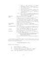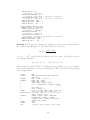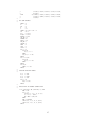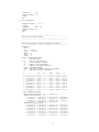
1
DFNLP: A Fortran Implementation of an
SQP-Gauss-Newton Algorithm
- User’s Guide, Version 2.0 -
Address:
Prof. Dr. K. Schittkowski
Department of Computer Science
University of Bayreuth
D - 95440 Bayreuth
Phone:
E-mail:
Web:
Date:
+49 921 553278
[email protected]
http://www.klaus-schittkowski.de
April, 2005
Abstract
The Fortran subroutine DFNLP solves constrained nonlinear programming
problems, where the objective function is of the form
- sum of squares of function values,
- sum of absolute function values,
- maximum of absolute function values,
- maximum of functions.
It is assumed that all individual problem functions are continuously differentiable. By introducing additional variables and constraints, the problem is
transformed into a general smooth nonlinear program which is then solved
by the SQP code NLPQLP, see Schittkowski [33], the most recent implementation with non-monotone line search (Dai, Schittkowski [3]). For the least
squares formulation, it can be shown that typical features of special purpose
algorithms are retained, i.e., a combination of a Gauss-Newton and a quasiNewton search direction. In this case, the additionally introduced variables
are eliminated in the quadratic programming subproblem, so that calculation
time is not increased significantly. Some comparative numerical results are
included, the usage of the code is documented, and an illustrative example is
presented.
Keywords: data fitting, constrained nonlinear least squares, min-max optimization,
L1 problems, Gauss-Newton method, SQP, sequential quadratic programming, nonlinear programming, numerical algorithms, Fortran codes
1
1
Introduction
Nonlinear least squares optimization is extremely important in many practical situations. Typical applications are maximum likelihood estimation, nonlinear regression,
data fitting, system identification, or parameter estimation, respectively. In these
cases, a mathematical model is available in form of one or several equations, and the
goal is to estimate some unknown parameters of the model. Exploited are available
experimental data, to minimize the distance of the model function, in most cases
evaluated at certain time values, from measured data at the same time values. An
extensive discussion of data fitting especially in case of dynamical systems is given
by Schittkowski [31].
The mathematical problem we want to solve, is given in the form
min
x ∈ IRn :
1
2
l
i=1
fi (x)2
gj (x) = 0 , j = 1, . . . , me ,
gj (x) ≥ 0 , j = me + 1, . . . , m ,
(1)
xl ≤ x ≤ xu .
It is assumed that f1 , . . ., fl and g1 , . . ., gm are continuously differentiable.
Although many nonlinear least squares programs were developed in the past, see
Hiebert [14] for an overview and numerical comparison, the author knows of only
very few programs that were written for the nonlinearly constrained case, e.g., the
code NLSNIP of Lindstr¨om [18]. However, the implementation of one of these or
any similar special purpose code requires a large amount additional efforts subject
to manpower and numerical experience.
In this paper, we consider the question how an existing nonlinear programming
code can be used to solve constrained nonlinear least squares problems in an efficient
and robust way. We will see that a simple transformation of the model under
consideration and subsequent solution by a sequential quadratic programming (SQP)
algorithm retains typical features of special purpose methods, i.e., the combination
of a Gauß-Newton search direction with a quasi-Newton correction. Numerical test
results indicate that the proposed approach is as efficient as the usage of special
purpose methods, although the required programming effort is negligible provided
that an SQP code is available.
The following section describes some basic features of least squares optimization,
especially some properties of Gauss-Newton and related methods. The transformation of a least squares problem into a special nonlinear program is described in
Section 3. We will discuss how some basic features of special purpose algorithms
are retained. The same ideas are extended to the constrained case in Section 4.
Alternativ norms are investigating in Section 5, i.e., the L∞ and the L1 norm. We
show that also in these cases, that simple transformations into smooth nonlinear
programs are possible. In Section 6, we summarize some comparative numerical
2
results on a large set of test problems. Section 7 contains a complete documentation
of the Fortran code and two examples.
DFNLP is applied in chemical engineering, pharmaceutics, mechanical engineering, and in natural sciences like biology, geology, ecology. Customers include
ACA, BASF, Battery Design, Bayer, Boehringer Ingelheim, Dow Chemical, GLM
Lasertechnik, Envirogain, Epcos, Eurocopter, Institutt for Energiteknikk, Novartis,
Oxeno, Prema, Prodisc, Springborn Laboratories, and dozens of academic research
institutions worldwide.
2
Least Squares Methods
First, we consider problems with respect to the L2 -norm, also called least squares
problems, where we omit constraints and bounds to simplify the notation,
min
1
2
l
i=1
fi (x)2
x ∈ IRn .
(2)
These problems possess a long history in mathematical programming and are extremely important in practice, particularly in nonlinear data fitting or maximum
likelihood estimation. In consequence, a large number of mathematical algorithms
is available for solving (2). To understand their basic features, we introduce the
notation F (x) = (f1 (x), . . . , fl (x))T and let
f (x) =
l
1
fi (x)2 .
2 i=1
Then
∇f (x) = ∇F (x)F (x)
(3)
defines the Jacobian of the objective function with ∇F (x) = (∇f1 (x), . . . , ∇fl (x)).
If we assume now that all functions f1 , . . ., fl are twice continuously differentiable,
we get the Hessian matrix of f by
∇2 f (x) = ∇F (x)∇F (x)T + B(x) ,
where
B(x) =
l
fi (x)∇2 fi (x) .
(4)
(5)
i=1
Proceeding from a given iterate xk , Newton’s method can be applied to (2) to
get a search direction dk ∈ IRn by solving the linear system
∇2 f (xk )d + ∇f (xk ) = 0
or, alternatively,
∇F (xk )∇F (xk )T d + B(xk )d + ∇F (xk )F (xk ) = 0 .
3
(6)
Assume that
F (x ) = (f1 (x ), . . . , fl (x ))T = 0
at an optimal solution x . A possible situation is a perfect fit where model function
values coincide with experimental data. Because of B(x ) = 0, we neglect matrix
B(xk ) in (6) for the moment, see also (5). Then (6) defines the so-called normal
equations of the linear least squares problem
min ∇F (xk )T d + F (xk )
d ∈ IRn .
(7)
A new iterate is obtained by xk+1 = xk + αk dk , where dk is a solution of (7) and
where αk denotes a suitable steplength parameter. It is obvious that a quadratic
convergence rate is achieved when starting sufficiently close to an optimal solution.
The above calculation of a search direction is known as the Gauss-Newton method
and represents the traditional way to solve nonlinear least squares problems, see
Bj¨orck [2] for more details. In general, the Gauss-Newton method possesses the
attractive feature that it converges quadratically although we only provide first
order information.
However, the assumptions of the convergence theorem of Gauss-Newton methods
are very strong and cannot be satisfied in real situations. We have to expect difficulties in case of non-zero residuals, rank-deficient Jacobian matrices, non-continuous
derivatives, and starting points far away from a solution. Further difficulties arise
when trying to solve large residual problems, where F (x )T F (x ) is not sufficiently
small, for example relative to ∇F (x ). Numerous proposals have been made in
the past to deal with this situation, and it is outside the scope of this section to give
a review of all possible attempts developed in the last 30 years. Only a few remarks
are presented to illustrate basic features of the main approaches, for further reviews
see Gill, Murray and Wright [10], Ramsin and Wedin [26], or Dennis [5].
A very popular method is known under the name Levenberg-Marquardt algorithm, see Levenberg [16] and Marquardt [20]. The key idea is to replace the Hessian
in (6) by a multiple of the identity matrix, say λk I, with a suitable positive factor
λk . We get a uniquely solvable system of linear equations of the form
∇F (xk )∇F (xk )T d + λk d + ∇F (xk )F (xk ) = 0 .
For the choice of λk and the relationship to so-called trust region methods, see
Mor´e [21].
A more sophisticated idea is to replace B(pk ) in (6) by a quasi-Newton-matrix Bk ,
see Dennis [4]. But some additional safeguards are necessary to deal with indefinite
matrices ∇F (xk )∇F (xk )T + Bk in order to get a descent direction. A modified
algorithm is proposed by Gill and Murray [9], where Bk is either a second-order
approximation of B(xk ), or a quasi-Newton matrix. In this case, a diagonal matrix
is added to ∇F (xk )∇F (xk )T +Bk to obtain a positive definite matrix. Lindstr¨om [17]
4
proposes a combination of a Gauss-Newton and a Newton method by using a certain
subspace minimization technique.
If, however, the residuals are too large, there is no possibility to exploit the
special structure and a general unconstrained minimization algorithm, for example
a quasi-Newton method, can be applied as well.
3
The SQP-Gauss-Newton Method
Many efficient special purpose computer programs are available to solve unconstrained nonlinear least squares problems. On the other hand, there exists a very
simple approach to combine the valuable properties of Gauss-Newton methods with
that of SQP algorithms in a straightforward way with almost no additional efforts.
We proceed from an unconstrained least squares problem in the form
min 12
l
i=1
fi (x)2
x ∈ IRn ,
(8)
see also (2). Since most nonlinear least squares problems are ill-conditioned, it is
not recommended to solve (8) directly by a general nonlinear programming method.
But we will see in this section that a simple transformation of the original problem
and its subsequent solution by an SQP method retains typical features of a special purpose code and prevents the need to take care of negative eigenvalues of an
approximated Hessian matrix as in the case of alternative approaches. The corresponding computer program can be implemented in a few lines provided that a SQP
algorithm is available.
The transformation, also described in Schittkowski [30, 31], consists of introducing l additional variables z = (z1 , . . . , zl )T and l additional equality constraints of
the form
(9)
fi (x) − zi = 0 , i = 1, . . . , l .
Then the equivalent transformed problem is
(x, z) ∈ IRn+l :
min
1 T
z z
2
F (x) − z = 0 ,
(10)
F (x) = (f1 (x), . . ., fl (x))T . We consider now (10) as a general nonlinear programming problem of the form
min f¯(¯
x)
n
¯
(11)
x¯ ∈ IR :
g¯(¯
x) = 0
with n
¯ = n + l, x¯ = (x, z), f¯(x, z) = 12 z T z, g¯(x, z) = F (x) − z, and apply an SQP
algorithm, see Spellucci [35], Stoer [36], or Schittkowski [28, 31]. The quadratic
programming subproblem is of the form
¯k d¯ + ∇f¯(¯
min 12 d¯T B
xk )T d¯
d¯ ∈ IRn¯ :
(12)
xk ) = 0 .
∇¯
g (¯
xk )T d¯ + g¯(¯
5
Here, x¯k = (xk , zk ) is a given iterate and
¯k =
B
Bk : Ck
CkT : Dk
(13)
with Bk ∈ IRn×n , Ck ∈ IRn×l , and Dk ∈ IRl×l , a given approximation of the Hessian
of the Lagrangian function L(¯
x, u) defined by
L(¯
x, u) = f¯(¯
x) − uT g¯(¯
x)
=
1 T
z z
2
Since
− uT (F (x) − z) .
∇x¯ L(¯
x, u) =
and
∇2x¯ L(¯
x, u)
=
with
B(x, u) = −
−∇F (x)u
z+u
B(x, u) : 0
0
: I
l
ui∇2 fi (x) ,
(14)
i=1
it seems to be reasonable to proceed now from a quasi-Newton matrix given by
¯k =
B
Bk : 0
0 : I
,
(15)
where Bk ∈ IRn×n is a suitable positive definite approximation of B(xk , uk ). Inser¯k into (12) leads to the equivalent quadratic programming subproblem
tion of this B
(d, e) ∈ IR
n+l
:
1 T
d Bk d + 12 eT e + zkT e
2
∇F (xk )T d − e + F (xk ) − zk
min
=0 ,
(16)
where we replaced d¯ by (d, e). Some simple calculations show that the solution of
the above quadratic programming problem is identified by the linear system
∇F (xk )∇F (xk )T d + Bk d + ∇F (xk )F (xk ) = 0 .
(17)
This equation is identical to (6), if Bk = B(xk ), and we obtain a Newton direction
for solving the unconstrained least squares problem (8).
Note that B(x) defined by (5) and B(x) defined by (14) coincide at an optimal
solution of the least squares problem, since F (xk ) = −uk . Based on the above
considerations, an SQP method can be applied to solve (10) directly. The quasi¯k are always positive definite, and consequently also the matrix
Newton-matrices B
Bk defined by (13). Therefore, we omit numerical difficulties imposed by negative
eigenvalues as found in the usual approaches for solving least squares problems.
6
When starting the SQP method, one could proceed from a user-provided initial
guess x0 for the variables and define
z0 = F (x0 ) ,
B0 =
μI : 0
0 : I
,
(18)
guaranteeing a feasible starting point x¯0 . The choice of B0 is of the form (15) and
allows a user to provide some information on the estimated size of the residuals,
if available. If it is known that the final norm F (x )T F (x ) is close to zero at
the optimal solution x , the user could choose a small μ in (18). At least in the
first iterates, the search directions are more similar to a Gauss-Newton direction.
Otherwise, a user could define μ = 1, if a large residual is expected.
¯k is decomposed in the form (15) and that B
¯k
Under the assumption that B
¯
be updated by the BFGS formula, then Bk+1 is decomposed in the form (15), see
Schittkowski [30]. The decomposition (15) is rarely satisfied in practice, but seems
to be reasonable, since the intention is to find a x ∈ IRn with
∇F (x )F (x ) = 0 ,
and ∇F (xk )T dk + F (xk ) is a Taylor approximation of F (xk+1 ). Note also that the
usual way to derive Newton’s method is to assume that the optimality condition is
satisfied for a certain linearization of a given iterate xk , and to use this linearized
system for obtaining a new iterate.
Example 3.1 We consider the banana function
f (x1 , x2 ) = 100(x2 − x1 2 )2 + (1 − x1 )2 .
When applying the nonlinear programming code NLPQLP of Schittkowski [28, 33],
an implementation of a general purpose SQP method, we get the iterates of Table 1
when starting at x0 = (−1.2, 1.0)T . The objective function is scaled by 0.5 to adjust
this factor in the least squares formulation (1). The last column contains an internal
stopping condition based on the optimality criterion, in our unconstrained case equal
to
|∇f (xk )Bk−1 ∇f (xk )|
with a quasi-Newton matrix Bk . We observe a very fast final convergence speed, but
a relatively large number of iterations.
The transformation discussed above, leads to the equivalent constrained nonlinear
programming problem
min z1 2 + z2 2
x1 , x2 , z1 , z2 : 10(x2 − x1 2 ) − z1 = 0 ,
1 − x1 − z2 = 0 .
7
Now NLPQLP computes the results of Table 2, where the second column shows in
addition the maximal constraint violation. Obviously, the convergence speed is much
faster despite of the inaccurate gradient evaluation by forward differences.
k
0
1
2
3
4
5
...
f (xk )
12.10
2.153
1.925
1.805
1.711
1.562
...
s(xk )
0.39 · 104
0.75 · 100
0.26 · 100
0.98 · 10−1
0.42 · 100
0.39 · 100
...
k
33
34
35
36
37
38
39
f (xk )
0.42 · 10−2
0.16 · 10−2
0.58 · 10−3
0.11 · 10−3
0.97 · 10−5
0.19 · 10−6
0.58 · 10−9
s(xk )
0.54 · 10−2
0.18 · 10−2
0.69 · 10−3
0.18 · 10−3
0.19 · 10−4
0.39 · 10−6
0.13 · 10−8
Table 1: NLP Formulation of Banana Function
k
0
1
2
f (xk )
12.10
0.96 · 10−14
0.81 · 10−14
r(xk )
0.0
48.3
0.13 · 10−6
s(xk )
24.8
0.23 · 10−6
0.16 · 10−13
Table 2: Least Squares Formulation of Banana Function
4
Constrained Least Squares Problems
Now we consider constrained nonlinear least squares problems
min
x ∈ IRn :
1
2
l
i=1
fi (x)2
gj (x) = 0 , j = 1, . . . , me ,
gj (x) ≥ 0 , j = me + 1, . . . , m ,
(19)
xl ≤ x ≤ xu .
A combination of the SQP method with the Gauss-Newton method is proposed by
Mahdavi-Amiri [19]. Lindstr¨om [18] developed a similar method based on an active
set idea leading to a sequence of equality constrained linear least squares problems.
A least squares code for linearly constrained problems was published by Hanson and
Krogh [13] that is based on a tensor model.
On the other hand, a couple of SQP codes are available for solving general smooth
nonlinear programming problems, for example VFO2AD (Powell [23]), NLPQLP
(Schittkowski [28, 33]), NPSOL (Gill, Murray, Saunders, Wright [11]), or DONLP2
8
(Spellucci [35]). Since most nonlinear least squares problems are ill-conditioned,
it is not recommended to solve (19) directly by a general nonlinear programming
method as shown in the previous section. The same transformation used before can
be extended to solve also constrained problems. The subsequent solution by an SQP
method retains typical features of a special purpose code and is implemented easily.
As outlined in the previous section, we introduce l additional variables z =
(z1 , . . . , zl )T and l additional nonlinear equality constraints of the form
fi (x) − zi = 0 ,
i = 1, . . ., l. The following transformed problem is to be solved by an SQP method,
min
1 T
z z
2
fi (x) − zi = 0 , i = 1, . . . , l ,
(x, z) ∈ IR
n+l
: gj (x) = 0 , j = 1, . . . , me ,
(20)
gj (x) ≥ 0 , j = me + 1, . . . , m ,
xl ≤ x ≤ xn .
In this case, the quadratic programming subproblem has the form
1
¯k (d, e) + z T e
(d, e)T B
k
2
T
∇fi (xk ) d − e + fi (xk ) − zik
min
= 0 , i = 1, . . . , l ,
(d, e) ∈ IRn+l : ∇gj (xk )T d + gj (xk ) = 0 , j = 1, . . . , me ,
(21)
∇gj (xk )T d + gj (xk ) ≥ 0 , j = me + 1, . . . , m ,
xl − xk ≤ d ≤ xu − xk .
It is possible to simplify the problem by substituting
e = ∇F (xk )T d + F (xk ) − zk ,
so that the quadratic programming subproblem depends on only n variables and
m linear constraints. This is an important observation from the numerical point of
view, since the computational effort to solve (21) reduces from the order of (n + l)3
to n3 , and the remaining computations in the outer SQP frame are on the order of
(n + l)2 . Therefore, the computational work involved in the proposed least squares
algorithm is comparable to the numerical efforts required by special purpose methods, at least if the number l of observations is not too large.
When implementing the above proposal, one has to be aware that the quadratic
programming subproblem is sometimes expanded by an additional variable δ, so
that some safeguards are required. Except for this limitation, the proposed transformation (20) is independent from the variant of the SQP method used, so that
available codes can be used in the form of a black box.
9
In principle, one could use the starting points proposed by (18). Numerical
experience suggests, however, starting from z0 = F (x0 ) only if the constraints are
satisfied at x0 ,
gj (x0 ) = 0 , j = 1, . . . , me ,
gj (x0 ) ≥ 0 , j = me + 1, . . . , m .
In all other cases, it is proposed to proceed from z0 = 0.
A final remark concerns the theoretical convergence of the algorithm. Since the
original problem is transformed into a general nonlinear programming problem, we
can apply all convergence results known for SQP methods. If an augmented Lagrangian function is preferred for the merit function, a global convergence theorem
is found in Schittkowski [27]. The theorem states that when starting from an arbitrary initial value, a Kuhn-Tucker point is approximated, i.e., a point satisfying the
necessary optimality conditions. If, on the other hand, an iterate is sufficiently close
to an optimal solution and if the steplength is 1, then the convergence speed of the
algorithm is superlinear, see Powell [24] for example. This remark explains the fast
final convergence rate one observes in practice.
The assumptions and are required by any special purpose algorithm in one or
another form. But in our case, we do not need any regularity conditions for the
function f1 , . . ., fl , i.e., an assumption that the matrix ∇F (xk ) is of full rank, to
adapt the mentioned convergence results to the least squares case. The reason is
found in the special form of the quadratic programming subproblem (21), since the
first l constraints are linearly independent and are also independent of the remaining
restrictions.
5
Alternative Norms
Except for of estimating parameters in the L2 -norm by minimizing the sum of squares
of residuals, it is sometimes desirable to change the norm, for example to reduce
the maximum distance of the model function from experimental data as much as
possible. Thus, we consider a possibility to minimize the sum of absolute values or
the maximum of absolute values as two additional alternative formulations. In both
cases, we get non-differentiable objective functions preventing the direct usage of
any of the algorithms mentioned in previous sections.
To overcome the difficulty, we transform the given problem into a smooth nonlinear programming problem that is solved then by any standard technique, for
instance an available SQP algorithm. In the first case, the original problem is given
in the form
min li=1 |fi (x)|
x ∈ IRn :
gj (x) = 0 , j = 1, . . . , me ,
gj (x) ≥ 0 , j = me + 1, . . . , m ,
xl ≤ x ≤ xu .
10
(22)
By introducing now l additional variables zi , i = 1, . . ., l, and 2l additional inequality
constraints, we get an equivalent smooth problem of the form
min
l
i=1
zi
gj (x) = 0 , j = 1, . . . , me ,
gj (x) ≥ 0 , j = me + 1, . . . , m ,
x ∈ IRn ,
:
z ∈ IRl
zi − fi (x) ≥ 0 , i = 1, . . . , l ,
(23)
zi + fi (x) ≥ 0 , i = 1, . . . , l ,
xl ≤ x ≤ xu .
From a solution of the extended problem, we get easily a solution of the original
one and vice versa. The transformed problem is differentiable, if we assume that
the model functions fi (x), i = 1, . . ., l, and the constraints gj (x), j = 1, . . ., m, are
continuously differentiable.
In a similar way, we transform a maximum-norm problem
min maxi=1,...,l |fi (x)|
x ∈ IRn :
gj (x) = 0 , j = 1, . . . , me ,
gj (x) ≥ 0 , j = me + 1, . . . , m ,
(24)
xl ≤ x ≤ xu
into an equivalent smooth nonlinear programming problem
min z
gj (x) = 0 , j = 1, . . . , me ,
gj (x) ≥ 0 , j = me + 1, . . . , m ,
x ∈ IRn ,
:
z ∈ IR
z − fi (x) ≥ 0 , i = 1, . . . , l ,
(25)
z + fi (x) ≥ 0 , i = 1, . . . , l ,
xl ≤ x ≤ xu
by introducing now only one additional variable.
Example 5.1 To test also a parameter estimation example, we consider a data
fitting problem defined by the model function
h(x, t) =
x1 (t2 + x2 t)
,
t2 + x3 t + x4
x = (x1 , . . . , x4 )T . There are two additional equality constraints
h(x, t1 ) − y1 = 0 ,
h(x, t11 ) − y11 = 0 .
11
The starting point is x0 = (0.25, 0.39, 0.415, 0.39)T . We apply the code DFNLP with
L1 , L2 , and L∞ norm and get the results of Table 3. Termination accuracy is set
to 10−7 according to the accuracy by which gradients are approximated. Here, f (x )
denotes the final objective function value, r(x ) the sum of constraint violations,
s(x ) the termination criterion, and ng the number of gradient evaluations until
convergence. In this case, we get three different solutions as must be expected.
norm f (x )
L1
0.082
L2
0.016
L∞ 0.021
x1
x2
x3
x4
r(x )
0.184 1.120 0.754 0.538 0.80 · 10−10
0.192 0.404 0.275 0.267 0.67 · 10−9
0.192 0.362 0.231 0.189 0.35 · 10−9
s(x )
0.28 · 10−7
0.35 · 10−7
0.12 · 10−7
ng
11
9
7
Table 3: Results of DFNLP for Different Norms
A valuable side-effect is the possibility, to apply the last transformation also to
min-max problems of the form
min maxi=1,...,l fi (x)
x ∈ IRn :
gj (x) = 0 , j = 1, . . . , me ,
gj (x) ≥ 0 , j = me + 1, . . . , m ,
(26)
xl ≤ x ≤ xu
into an equivalent smooth nonlinear program
min z
gj (x) = 0 , j = 1, . . . , me ,
x ∈ IRn ,
: gj (x) ≥ 0 , j = me + 1, . . . , m ,
z ∈ IR
z − fi (x) ≥ 0 , i = 1, . . . , l ,
(27)
xl ≤ x ≤ xu
by introducing now one additional variable and l additional inequality constraints.
In contrast to (26), problem (27) is now a smooth nonlinear optimization problem
assuming that all model functions are smooth.
12
6
Performance Evaluation
Since the proposed transformation does not depend on constraints, we consider now
the unconstrained least squares problem
min 12 li=1 fi (x)2
x ∈ IR :
xl ≤ x ≤ xu .
n
(28)
We assume that all functions fi (x), i = 1, . . ., l, are continuously differentiable.
Efficient and reliable least squares algorithms were implemented mainly in the 1960s
and 1970s, see for example Fraley [8] for a review. An early comparative study of
13 codes was published by Bard [1]. In most cases, mathematical algorithms are
based on the Gauss-Newton method, see Section 2. When developing and testing
new implementations, the authors used standard test problems, which have been
collected from literature and which do not possess a data fitting structure in most
cases, see Dennis et al. [6], Hock and Schittkowski [15], or Schittkowski [29].
Our intention is to present a comparative study of some least squares codes, when
applied to a set of data fitting problems. Test examples are given in form of analytical
functions to avoid additional side effects introduced by round-off or integration errors
as, e.g., in the case of dynamical systems. We proceed from a subset of the parameter
estimation problems listed in Schittkowski [31], a set of 143 least squares functions.
More details, in particular the corresponding model functions, data, and results,
are found in the database of the software system EASY-FIT [31, 32], which can be
downloaded from the home page of the author1 . Derivatives are evaluated by the
automatic differentiation tool PCOMP, see Dobmann et al. [7]. The following least
squares routines are executed to solve the test problems mentioned before:
DFNLP: By transforming the original problem into a general nonlinear programming problem in a special way, typical features of a Gauss-Newton and quasi-Newton
least squares method are retained, as outlined in the previous sections. The resulting optimization problem is solved by a standard sequential quadratic programming
code called NLPQLP, see Schittkowski [28, 33].
NLSNIP: The code is a special purpose implementation for solving constrained
nonlinear least squares problems by a combination of Gauss-Newton, Newton, and
quasi-Newton techniques, see Lindstr¨om [17, 18].
DN2GB: The subroutine is a frequently used unconstrained least squares algorithm developed by Dennis et al. [6]. The mathematical method is also based on a
combined Gauss-Newton and quasi-Newton approach.
DSLMDF: First, successive line searches are performed along the unit vectors by
comparing function values only. The one-dimensional minimization uses successive quadratic interpolation. After a search cycle, the Gauss-Newton-type method
DFNLP is executed with a given number of iterations. If a solution is not obtained
1
http://www.klaus-schittkowski.de/
13
with sufficient accuracy, the direct search along axes is repeated, see Nickel [22] for
details.
All algorithms are capable of taking upper and lower bounds of the variables into
account, but only DFNLP and NLSNIP are able to solve also constrained problems.
The optimization routines are executed with the same set of input parameters,
although we know that in one or another case, these tolerances can be adapted to
a special situation leading to better individual results. Termination tolerance for
DFNLP is 10−10 . DN2GB is executed with tolerances 10−9 and 10−7 for the relative
function and variable convergence. NLSNIP uses a tolerance of 10−10 for the relative
termination criteria and 10−8 for the absolute stopping condition. The total number
of iterations is bounded by 1,000 for all three algorithms. The code DSLMDF is not
allowed to perform more than 100 outer iteration cycles with a termination accuracy
of 10−9 for the local search step performed by DFNLP. The search algorithm needs
at most 50 function evaluations for each line search with reduction factor of 2.0 and
an initial steplength of 0.1.
In some situations, an algorithm is unable to stop at the same optimal solution
obtained by the other ones. There are many possible reasons, for example termination at a local solution, internal instabilities, or round-off errors. Thus, we need a
decision when an optimization run is considered to be a successful one or not. We
claim that successful termination is obtained if the total residual norm differs at
most by 1 % from the best value obtained by all four algorithms, or, in case of a
problem with zero residuals, is less than 10−7 . The percentage of successful runs is
listed in Table 4, where the corresponding column is denoted by succ.
Comparative performance data are evaluated only for those test problems which
are successfully solved by all four algorithms, altogether 95 problems. The corresponding mean values for number of function and gradient evaluations are denoted
by nf and ng and are also shown in Table 4.
Although the number of test examples is too low to obtain statistically relevant
results, we get the impression that the codes DN2GB and NLSNIP behave best
with respect to efficiency. DFNLP and DN2GB are somewhat more reliable than
the others subject to convergence towards a global solution. The combined method
DSLMDF needs more function evaluations because of the successive line search
steps. However, none of the four codes tested is able to solve all problems within
the required accuracy.
14
code
DFNLP
NLSNIP
DN2GB
DSLMDF
succ
94.4 %
87.4 %
93.0 %
77.6 %
nf
30.2
26.5
27.1
290.9
ng
19.6
17.0
19.2
16.6
Table 4: Performance Results for Explicit Test Problems
7
Program Documentation
DFNLP is implemented in form of a Fortran subroutine. Model functions and
gradients are called by subroutine calls or, alternatively, by reverse communication.
In the latter case, the user has to provide functions and gradients in the same
program which executes DFNLP, according to the following rules:
1. Choose starting values for the variables to be optimized, and store them in
the first column of X.
2. Compute objective and all constraint function values, store them in RES and
G, respectively.
3. Compute gradients of objective function and all constraints, and store them
in DRES and DG, respectively. The J-th row of DG contains the gradient of
the J-th constraint, J=1,...,M.
4. Set IFAIL=0 and execute DFNLP.
5. If DFNLP returns with IFAIL=-1, compute objective function and constraint
values subject to variable values found in X, store them in RES and G, and
call DFNLP again.
6. If DFNLP terminates with IFAIL=-2, compute gradient values with respect to
the variables stored in X, and store them in DRES and DG. Only derivatives
for active constraints, ACTIVE(J)=.TRUE., need to be computed. Then call
DFNLP again.
7. If DFNLP terminates with IFAIL=0, the internal stopping criteria are satisfied. In case of IFAIL>0, an error occurred.
Note that RES, G, DRES, and DG contain the transformed data and must be
set according to the specific model variant chosen. If analytical derivatives are not
available, simultaneous function calls can be used for gradient approximations, for
example by forward differences, two-sided differences, or even higher order formulae.
15
Usage:
CALL
/
/
/
DFNLP(MODEL,M,ME,LMMAX,L,N,LNMAX,LMNN2,LN,X,F,
RES,G,DRES,DG,U,XL,XU,ACC,ACCQP,RESSIZ,MAXFUN,
MAXIT,MAX NM,TOL NM,IPRINT,MODE,IOUT,IFAIL,
WA,LWA,KWA,LKWA,ACTIVE,LACTIV,QPSOLVE)
Definition of the parameters:
MODEL :
Optimization model, i.e.,
1 - L1 norm, i.e., min li=1 |fi (x)|,
2 - L2 norm, i.e., min 12 li=1 fi (x)2 ,
3 - L∞ norm, i.e., min maxi=1,...,l |fi (x)|,
M:
ME :
LMMAX :
L:
N:
LNMAX :
LMNN2 :
LN :
X(LN) :
F(L) :
4 - min-max problem, i.e., min maxi=1,...,l fi (x).
Number of constraints.
Number of equality constraints.
Row dimension of array DG for Jacobian of constraints. LMMAX must be at least one and greater or equal to
M + L + L, if MODEL=1,3,
M + L,
if MODEL=2,4.
Number of terms in objective function.
Number of variables.
Row dimension of C and dimension of DRES. LNMAX must
be at least two and greater than
N + L, if MODEL=1,2,
N + 1, if MODEL=3,4.
Must be equal to
M + 2N + 4L + 2, if MODEL=1,
M + 2N + 3L + 2, if MODEL=2,
M + 2N + 2L + 4, if MODEL=3,
M + 2N + L + 4,
if MODEL=4
when calling DFNLP.
Must be set to
N + L, if MODEL=1,2,
N + 1, if MODEL=3,4.
Initially, the first N positions of X have to contain starting
values for the optimal solution. On return, X is replaced by
the current iterate. In the driving program the dimension of X
should be equal to LNMAX.
On return, F contains the final objective function values by
which the function to be minimized is composed of.
16
RES :
G(LMMAX) :
DRES(LMMAX) :
DG(LMMAX,LN) :
U(LMNN2) :
XL(LN),XU(LN) :
ACC :
ACCQP :
RESSIZE :
MAXFUN :
MAXIT :
MAX NM :
TOL NM :
On return, RES contains the final objective function value.
On return, the first M coefficients of G contain the constraint
function values at the final iterate X. In the driving program,
the dimension of G should be equal to LMMAX.
On return, DRES contains the gradient of the transformed objective function subject to the final iterate X.
On return, DG contains the gradients of the active constraints
(ACTIVE(J)=.true.) at a current iterate X subject to the
transformed problem. The remaining rows are filled with previously computed gradients. In the driving program, the row
dimension of DG has to be equal to LMMAX.
On return, U contains the multipliers with respect to the iterate
stored in X. The first M coefficients contain the multipliers of
the M nonlinear constraints followed by the multipliers of the
lower and upper bounds. At an optimal solution, all multipliers
of inequality constraints should be nonnegative.
On input, the one-dimensional arrays XL and XU must contain
the upper and lower bounds of the variables. Only the first
N positions need to be defined, the bounds for the artificial
variables are set by DFNLP.
The user has to specify the desired final accuracy (e.g. 1.0D-7).
The termination accuracy should not be much smaller than the
accuracy by which gradients are computed.
The tolerance is needed for the QP solver to perform several
tests, for example whether optimality conditions are satisfied
or whether a number is considered as zero or not. If ACCQP
is less or equal to zero, then the machine precision is computed
by DFNLP20 and subsequently multiplied by 1.0D+4.
Guess for the approximate size of the residuals of the least
squares problem at the optimal solution (MODEL=2), must
be positive.
The integer variable defines an upper bound for the number of
function calls during the line search (e.g. 20).
Maximum number of outer iterations, where one iteration corresponds to one formulation and solution of the quadratic programming subproblem, or, alternatively, one evaluation of gradients (e.g. 100).
Stack size for storing merit function values at previous iterations for non-monotone line search (e.g. 10). If MAX NM=0,
monotone line search is performed.
Relative bound for increase of merit function value, if line
search is not successful during the very first step (e.g. 0.1).
TOL NM must not be negative.
17
IPRINT :
MODE :
IOUT :
IFAIL :
Specification of the desired output level, passed to NLPQLP
together with the transformed problem:
0 - No output of the program.
1 - Only a final convergence analysis is given.
2 - One line of intermediate results is printed in each iteration.
3 - More detailed information is printed in each iteration
step, e.g., variable, constraint and multiplier values.
4 - In addition to ’IPRINT=3’, merit function and
steplength values are displayed during the line search.
The parameter specifies the desired version of DFNLP.
0 - Normal execution, function and gradient values passed
through subroutine calls.
2 - The user wants to perform reverse communication.
In this case, IFAIL must be set to 0 initially and
RES, G, DRES, DG contain the corresponding function and gradient values of the transformed problem.
If DFNLP returns with IFAIL=-1, new function values
have to be computed subject to the variable X, stored
in RES and G, and DFNLP must be called again. If
DFNLP returns with IFAIL=-2, new gradient values
have to be computed, stored in DRES and DG, and
DFNLP must be called again. Only gradients of active
constraints (ACTIVE(J)=.TRUE.) need to be recomputed
Integer indicating the desired output unit number, i.e., all
write-statements start with ’WRITE(IOUT,... ’.
The parameter shows the reason for terminating a solution process. Initially IFAIL must be set to zero. On return IFAIL could
contain the following values:
-2 - In case of MODE=2, compute gradient values,
store them in DRES and DG, and call DFNLP
again.
-1 - In case of MODE=2, compute objective function
and all constraint values, store them in RES and
G, and call DFNLP again.
0 - The optimality conditions are satisfied.
1 - The algorithm stopped after MAXIT iterations.
2 - The algorithm computed an uphill search direction.
3 - Underflow occurred when determining a new approximation matrix for the Hessian of the Lagrangian.
4 - The line search could not be terminated successfully.
5 - Length of a working array is too short. More
detailed error information is obtained with
’IPRINT>0’.
18
6
WA(LWA) :
LWA :
KWA(LKWA) :
LKWA :
ACTIVE(LACTIV) :
LACTIV :
QPSOLVE :
-
There are false dimensions, for example
M>MMAX, N≥NMAX, or MNN2=M+N+N+2.
7 - The search direction is close to zero, but the current
iterate is still infeasible.
8 - The starting point violates a lower or upper bound.
9 - Wrong input parameter, i.e., MODE, LDL decomposition in D and C (in case of MODE=1),
IPRINT, IOUT, ...
>100 - The solution of the quadratic programming subproblem has been terminated with an error message
IFQL and IFAIL is set to IFQL+100.
WA is a real working array of length LWA.
Length of the real working array WA. LWA must be at least
7*LNMAX*LNMAX/2+34*LNMAX+9*LMMAX+200.
The working array length was computed under the assumption, that LNMAX=L+N+1, LMMAX=L+M+1, and that the
quadratic programming subproblem is solved by subroutine QL
or LSQL, respectively, see Schittkowski [34].
KWA is an integer working array of length LKWA.
Length of the integer working array KWA. LKWA should be
at least LN+15.
The logical array indicates constraints, which DFNLP considers
to be active at the last computed iterate, i.e., G(J,X) is active,
if and only if ACTIVE(J)=.TRUE., J=1,...,M.
Length of the logical array ACTIVE. The length LACTIV of
the logical array should be at least 2*(M+L+L)+10.
External subroutine to solve the quadratic programming subproblem. The calling sequence is
CALL QPSOLVE(M,ME,MMAX,N,NMAX,MNN,C,D,A,B,
/
XL,XU,X,U,EPS,MODE,IOUT,IFAIL,IPRINT,
/
WAR,LWAR,IWAR,LIWAR)
For more details about the choice and dimensions of arguments,
see [33].
All declarations of real numbers must be done in double precision. In case of
normal execution (MODE=0), a user has to provide the following two subroutines
for function and gradient evaluations.
SUBROUTINE DFFUNC(J,N,F,X)
Definition of the parameters:
J:
N:
F:
X(N) :
Index of function to be evaluated.
Number of variables and dimension of X.
If J>0, the J-th term of the objective function is to computed,
if J<0, the -J-th constraint function value and stored in F.
When calling DFFUNC, X contains the actual iterate.
19
SUBROUTINE DFGRAD(J,N,DF,X)
Definition of the parameters:
J:
N:
DF :
X(N) :
Index of function for which the gradient is to be evaluated.
Number of variables and dimension of DF and X, respectively.
If J>0, the gradient of the J-th term of the objective function
is to computed, if J<0, the gradient of the -J-th constraint
function value. In both cases, the gradient is to be stored in
DF.
When calling DFGRAD, X contains the actual iterate.
In case of MODE=2, one has to declare dummy subroutines with the names DFFUNC and DFGRAD. Subroutine DFNLP is to be linked with the user-provided
main program, the two subroutines DFFUNC and DFGRAD, the new SQP code
NLPQLP, see Schittkowski [34], and the quadratic programming code QL, see Schittkowski [34]. In case of least squares optimization and a larger number of terms in
the objective function, the code QL should be replaced by the code LSQL which
takes advantage of the special structure of the subproblem.
Some of the termination reasons depend on the accuracy used for approximating gradients. If we assume that all functions and gradients are computed within
machine precision and that the implementation is correct, there remain only the
following possibilities that could cause an error message:
1. The termination parameter ACC is too small, so that the numerical algorithm
plays around with round-off errors without being able to improve the solution.
Especially the Hessian approximation of the Lagrangian function becomes unstable in this case. A straightforward remedy is to restart the optimization
cycle again with a larger stopping tolerance.
2. The constraints are contradicting, i.e., the set of feasible solutions is empty.
There is no way to find out, whether a general nonlinear and non-convex set
possesses a feasible point or not. Thus, the nonlinear programming algorithms
will proceed until running in any of the mentioned error situations. In this
case, there the correctness of the model must be checked very carefully.
3. Constraints are feasible, but some of them there are degenerate, for example
if some of the constraints are redundant. One should know that SQP algorithms require satisfaction of the so-called constraint qualification, i.e., that
gradients of active constraints are linearly independent at each iterate and in
a neighborhood of the optimal solution. In this situation, it is recommended
to check the formulation of the model.
However some of the error situations do also occur, if because of wrong or nonaccurate gradients, the quadratic programming subproblem does not yield a descent
20
direction for the underlying merit function. In this case, one should try to improve
the accuracy of function evaluations, scale the model functions in a proper way, or
start the algorithm from other initial values.
Example 7.1 To give a simple example how to organize the code in case of two
explicitly given functions, we consider again Rosenbrock’s banana function, see Example 3.1 or test problem TP1 of Hock and Schittkowski [15]. The problem is
min 100(x2 − x21 )2 + (1 − x1 )2
x1 , x2 ∈ IR : −1000 ≤ x1 ≤ 1000
(29)
−1000 ≤ x2 ≤ 1000
The Fortran source code for executing NLPQLP is listed below. Gradients are computed analytically, but a piece of code is is shown in form of comments for approximating them by forward differences. In case of activating numerical gradient
evaluation, some tolerances should be adapted, i.e., ACC=1.0D-8 and RESSIZ =
1.0D-8.
C
C
C
C
C
IMPLICIT NONE
INTEGER
NMAX, MMAX, LMAX, LMMAX, LNMAX, LMNNX2, LWA,
/
LKWA, LACTIV
PARAMETER
(NMAX
= 2, MMAX = 0, LMAX = 2)
PARAMETER
(LMMAX = MMAX + 2*LMAX,
/
LNMAX = NMAX + LMAX + 1,
/
LMNNX2 = MMAX + 2*NMAX + 4*LMAX + 4,
/
LWA
= 7*LNMAX*LNMAX/2 + 34*LNMAX + 9*LMMAX
/
+ 200,
/
LKWA
= LNMAX + 15,
/
LACTIV = 2*LMMAX + 10)
INTEGER
M, ME, N, L, LMNN2, MAXFUN, MAXIT, MAX_NM,
/
IPRINT, MODE, IOUT, IFAIL, KWA, I, MODEL, LN
DOUBLE PRECISION X, F, RES, G, DRES, DG, U, XL, XU, ACC, ACCQP,
/
RESSIZ, TOL_NM, WA
DIMENSION
X(LNMAX), F(LMAX), G(LMMAX), DRES(LNMAX),
/
DG(LMMAX,LNMAX), U(LMNNX2), XL(LNMAX),
/
XU(LNMAX), WA(LWA), KWA(LKWA), ACTIVE(LACTIV)
LOGICAL
ACTIVE
EXTERNAL
LSQL, QL, DFFUNC, DFGRAD
SET SOME CONSTANTS
M
ME
N
L
ACC
ACCQP
RESSIZ
TOL_NM
MAXFUN
MAXIT
MAX_NM
IPRINT
IOUT
IFAIL
=
=
=
=
=
=
=
=
=
=
=
=
=
=
0
0
2
2
1.0D-12
1.0D-14
1.0D0
0.0
10
100
0
2
6
0
EXECUTE DFNLP
21
C
MODE
= 0
DO MODEL=1,4
WRITE (IOUT,*) ’*** MODEL =’,MODEL
IF (MODEL.EQ.1) THEN
LN = N + L
LMNN2 = M + 2*N + 4*L + 2
ENDIF
IF (MODEL.EQ.2) THEN
LN = N + L
LMNN2 = M + 2*N + 3*L + 2
ENDIF
IF (MODEL.EQ.3) THEN
LN = N + 1
LMNN2 = M + 2*N + 2*L + 4
ENDIF
IF (MODEL.EQ.4) THEN
LN = N + 1
LMNN2 = M + 2*N + L + 4
ENDIF
X(1) = -1.2D0
X(2) = 1.0D0
DO I = 1,N
XL(I) = -1000.0D0
XU(I) = 1000.0D0
ENDDO
IF (MODEL.EQ.2) THEN
CALL DFNLP(MODEL, M, ME, LMMAX, L, N, LNMAX, LMNN2, LN, X,
/
F, RES, G, DRES, DG, U, XL, XU, ACC, ACCQP,
/
RESSIZ, MAXFUN, MAXIT, MAX_NM, TOL_NM, IPRINT,
/
MODE, IOUT, IFAIL, WA, LWA, KWA, LKWA, ACTIVE,
/
LACTIV, LSQL)
ELSE
CALL DFNLP(MODEL, M, ME, LMMAX, L, N, LNMAX, LMNN2, LN, X,
/
F, RES, G, DRES, DG, U, XL, XU, ACC, ACCQP,
/
RESSIZ, MAXFUN, MAXIT, MAX_NM, TOL_NM, IPRINT,
/
MODE, IOUT, IFAIL, WA, LWA, KWA, LKWA, ACTIVE,
/
LACTIV, QL)
ENDIF
ENDDO
C
C
C
END OF MAIN PROGRAM
C
C
C
COMPUTE FUNCTION VALUES
C
C
C
EVALUATION OF PROBLEM FUNCTIONS
C
C
C
END OF DFFUNC
STOP
END
SUBROUTINE DFFUNC(J, N, F, X)
IMPLICIT NONE
INTEGER
J, N
DOUBLE PRECISION F, X(N)
IF (J.EQ.1) THEN
F = 10.0D0*(X(2) - X(1)**2)
ELSE
F = 1.0D0 - X(1)
ENDIF
RETURN
END
22
C
C
C
EVALUATION OF GRADIENTS
C
C
C
ANALYTICAL DERIVATIVES
C
C
C
END OF DFGRAD
SUBROUTINE DFGRAD(J, N, DF, X)
IMPLICIT NONE
INTEGER
J, N, I
DOUBLE PRECISION DF(N), X(N), EPS, FI, FEPS
IF (J.EQ.1) THEN
DF(1) = -2.0D1*X(1)
DF(2) = 10.0D0
ELSE
DF(1) = -1.0D0
DF(2) = 0.0D0
ENDIF
RETURN
END
The following output should appear on screen, mainly generated by NLPQLP:
-------------------------------------------------------------------START OF DATA FITTING ALGORITHM
--------------------------------------------------------------------------------------------------------------------------------------START OF THE SEQUENTIAL QUADRATIC PROGRAMMING ALGORITHM
-------------------------------------------------------------------PARAMETERS:
MODE = 1
ACC =
0.1000D-13
SCBOU =
0.1000D+31
MAXFUN = 10
MAXIT = 100
IPRINT =
2
OUTPUT IN THE FOLLOWING ORDER:
IT
- ITERATION NUMBER
F
- OBJECTIVE FUNCTION VALUE
SCV
- SUM OF CONSTRAINT VIOLATION
NA
- NUMBER OF ACTIVE CONSTRAINTS
I
- NUMBER OF LINE SEARCH ITERATIONS
ALPHA - STEPLENGTH PARAMETER
DELTA - ADDITIONAL VARIABLE TO PREVENT INCONSISTENCY
KT
- KUHN-TUCKER OPTIMALITY CRITERION
IT
F
SCV
NA I
ALPHA
DELTA
KT
-------------------------------------------------------------------1 0.12100005D+02 0.00D+00
2 0 0.00D+00 0.00D+00 0.24D+02
2 0.10311398D-26 0.48D+02
2 1 0.10D+01 0.00D+00 0.35D-12
3 0.24527658D-25 0.36D-14
2 1 0.10D+01 0.00D+00 0.49D-25
* FINAL CONVERGENCE ANALYSIS
OBJECTIVE FUNCTION VALUE: F(X) = 0.24527658D-25
APPROXIMATION OF SOLUTION: X =
0.10000000D+01 0.10000000D+01 -0.49737992D-13
APPROXIMATION OF MULTIPLIERS: U =
0.47331654D-27 -0.11410084D-25 0.00000000D+00
0.00000000D+00 0.00000000D+00 0.00000000D+00
0.00000000D+00 0.00000000D+00
23
0.21582736D-12
0.00000000D+00
0.00000000D+00
CONSTRAINT VALUES: G(X) =
-0.35527137D-14 -0.10955700D-25
DISTANCE FROM LOWER BOUND: XL-X =
-0.10010000D+04 -0.10010000D+04 -0.10000000D+31 -0.10000000D+31
DISTANCE FROM UPPER BOUND: XU-X =
0.99900000D+03 0.99900000D+03 0.10000000D+31 0.10000000D+31
NUMBER OF FUNC-CALLS: NFUNC =
3
NUMBER OF GRAD-CALLS: NGRAD =
3
NUMBER OF QL-CALLS:
NQL
=
3
* FINAL CONVERGENCE ANALYSIS OF DFNLP
RESIDUAL: RES(X) = 0.49421347D-25
OBSERVATION FUNCTION VALUES: F(X) =
-0.53290705D-13 0.21582736D-12
APPROXIMATION OF SOLUTION: X =
0.10000000D+01 0.10000000D+01
APPROXIMATION OF MULTIPLIERS: U =
0.00000000D+00 0.00000000D+00 0.00000000D+00
NUMBER OF DFFUNC-CALLS: NFUNC =
4
NUMBER OF DFGRAD-CALLS: NGRAD =
3
NUMBER OF QL-CALLS:
NQL
=
3
0.00000000D+00
Example 7.2 To present a data fitting example and also reverse communication,
we consider again Example 5.1. The model function is given by
h(x, t) =
x1 (t2 + x2 t)
,
t2 + x3 t + x4
x = (x1 , . . . , x4 )T , and the data are shown in the code below. In addition, we have
two equality constraints
h(x, t1 ) − y1 = 0 ,
h(x, t11 ) − y11 = 0 .
Some results are found in Table 3 for different norms. In this case, we use only the
least squares formulation in reverse communication. The code and the corresponding
screen output follow.
IMPLICIT
NONE
INTEGER
NMAX, MMAX, LMAX, LMMAX, LNMAX, LMNN2X, LWA,
/
LKWA, LACTIV
PARAMETER
(NMAX = 4, MMAX = 2, LMAX = 11)
PARAMETER
(LMMAX = MMAX + 2*LMAX,
/
LNMAX = NMAX + 2*LMAX + 1,
/
LMNN2X = MMAX + 2*NMAX + 3*LMAX + 2,
/
LWA
= 7*LNMAX*LNMAX/2 + 34*LNMAX + 9*LMMAX
/
+ 200,
/
LKWA = LNMAX + 15,
/
LACTIV = 2*LMMAX + 10)
INTEGER
M, ME, N, L, LMNN2, MAXFUN, MAXIT, IPRINT, MODE,
/
MAX_NM, IOUT, IFAIL, KWA, I, MODEL, LN, J
DOUBLE PRECISION X, F, RES, G, DRES, DG, U, XL, XU, ACC, ACCQP,
/
RESSIZ, TOL_NM, WA, EPS, T, Y, W
DIMENSION
X(LNMAX), F(LMAX), G(LMMAX), DRES(LNMAX),
/
DG(LMMAX,LNMAX), U(LMNN2X), XL(LNMAX),
/
XU(LNMAX), WA(LWA), KWA(LKWA), ACTIVE(LACTIV),
/
T(LMAX),Y(LMAX), W(NMAX)
LOGICAL
ACTIVE
EXTERNAL
LSQL
DATA
T/0.0625D0,0.0714D0,0.0823D0,0.1000D0,0.1250D0,
24
/
/
DATA
/
/
0.1670D0,0.2500D0,0.5000D0,1.0000D0,2.0000D0,
4.0000D0/
Y/0.0246D0,0.0235D0,0.0323D0,0.0342D0,0.0456D0,
0.0627D0,0.0844D0,0.1600D0,0.1735D0,0.1947D0,
0.1957D0/
C
C
C
SET SOME CONSTANTS
C
C
C
STARTING VALUES AND BOUNDS
C
C
C
EXECUTE DFNLP IN REVERSE COMMUNICATION
MODEL = 2
M
= 2
ME
= 2
N
= 4
L
= 11
LMNN2 = M + 2*N + 3*L + 2
LN
= N + L
ACC
= 1.0D-14
ACCQP = 1.0D-14
RESSIZ = 1.0D-4
TOL_NM = 0.0
MAXFUN = 20
MAXIT = 100
MAX_NM = 0
IPRINT = 2
MODE
= 2
IOUT
= 6
IFAIL = 0
DO J = 1,L
DO I=1,LN
DG(J,I) = 0.0
ENDDO
DG(J,N+J) = -1.0D0
ENDDO
DO J = L+1,L+M
DO I=1,LN
DG(J,I) = 0.0D0
ENDDO
ENDDO
DO I=1,LN
DRES(I) = 0.0D0
ENDDO
X(1) = 0.25D0
X(2) = 0.39D0
X(3) = 0.415D0
X(4) = 0.39D0
DO I = 1,N
XL(I) = 0.0D0
XU(I) = 1.0D5
ENDDO
1 IF ((IFAIL.EQ.0).OR.(IFAIL.EQ.-1)) THEN
RES = 0.0D0
DO J = 1,L
CALL H(T(J), Y(J), N, X, G(J))
G(J) = G(J) - X(N+J)
RES = RES + X(N+J)**2
ENDDO
RES = 0.5D0*RES
CALL H(T(1), Y(1), N, X, G(L+1))
CALL H(T(L), Y(L), N, X, G(L+2))
ENDIF
25
2 IF ((IFAIL.EQ.0).OR.(IFAIL.EQ.-2)) THEN
DO J = 1,L
CALL DH(T(J), N ,X, W)
DO I=1,N
DG(J,I) = W(I)
ENDDO
ENDDO
CALL DH(T(1), N, X, W)
DO I=1,N
DG(L+1,I) = W(I)
ENDDO
CALL DH(T(L), N, X, W)
DO I=1,N
DG(L+2,I) = W(I)
ENDDO
DO I=1,L
DRES(N+I) = X(N+I)
ENDDO
ENDIF
C
C
C
CALL DFNLP
C
C
C
END OF MAIN PROGRAM
C
C
C
DATA FITTING FUNCTION
C
C
C
C
C
C
C
C
C
C
CALL DFNLP(MODEL, M, ME, LMMAX, L, N, LNMAX, LMNN2, LN, X, F,
/
RES, G, DRES, DG, U, XL, XU, ACC, ACCQP, RESSIZ,
/
MAXFUN, MAXIT, MAX_NM, TOL_NM, IPRINT, MODE, IOUT,
/
IFAIL, WA, LWA, KWA, LKWA, ACTIVE, LACTIV, LSQL)
IF (IFAIL.EQ.-1) GOTO 1
IF (IFAIL.EQ.-2) GOTO 2
STOP
END
SUBROUTINE
IMPLICIT
INTEGER
DOUBLE PRECISION
H(T, Y, N ,X, F)
NONE
N
T, Y, X(N), F
F = X(1)*T*(T + X(2))/(T**2 + X(3)*T + X(4)) - Y
RETURN
END
MODEL DERIVATIVES
SUBROUTINE
IMPLICIT
INTEGER
DOUBLE PRECISION
DF(1)
DF(2)
DF(3)
DF(4)
=
=
=
=
DH(T, N ,X, DF)
NONE
N
T, X(N), DF(N)
T*(T + X(2))/(T**2 + X(3)*T + X(4))
X(1)*T/(T**2 + X(3)*T + X(4))
-X(1)*T**2*(T + X(2))/(T**2 + X(3)*T + X(4))**2
-X(1)*T*(T + X(2))/(T**2 + X(3)*T + X(4))**2
RETURN
END
DUMMY FOR FUNCTIONS
SUBROUTINE DFFUNC(J, N, F, X)
INTEGER
J, N
26
C
C
C
DIMENSION
DOUBLE PRECISION
RETURN
END
X(N)
F, X
DUMMY FOR GRADIENTS
SUBROUTINE DFGRAD(J, N, DF, X)
INTEGER
J, N
DIMENSION
X(N), DF(N)
DOUBLE PRECISION DF, X
RETURN
END
-------------------------------------------------------------------START OF DATA FITTING ALGORITHM
--------------------------------------------------------------------------------------------------------------------------------------START OF THE SEQUENTIAL QUADRATIC PROGRAMMING ALGORITHM
-------------------------------------------------------------------PARAMETERS:
MODE = 3
ACC =
0.1000D-13
SCBOU =
0.1000D+31
MAXFUN = 20
MAXIT = 100
IPRINT =
2
OUTPUT IN THE FOLLOWING ORDER:
IT
- ITERATION NUMBER
F
- OBJECTIVE FUNCTION VALUE
SCV
- SUM OF CONSTRAINT VIOLATION
NA
- NUMBER OF ACTIVE CONSTRAINTS
I
- NUMBER OF LINE SEARCH ITERATIONS
ALPHA - STEPLENGTH PARAMETER
DELTA - ADDITIONAL VARIABLE TO PREVENT INCONSISTENCY
KT
- KUHN-TUCKER OPTIMALITY CRITERION
IT
F
SCV
NA I
ALPHA
DELTA
KT
-------------------------------------------------------------------1 0.00000000D+00 0.25D+00 13 0 0.00D+00 0.00D+00 0.11D-02
2 0.11432789D-04 0.18D+00 13 2 0.24D+00 0.00D+00 0.80D-03
3 0.20506917D-03 0.38D-01 13 1 0.10D+01 0.00D+00 0.21D-03
4 0.20655267D-03 0.38D-02 13 1 0.10D+01 0.00D+00 0.24D-04
5 0.20640309D-03 0.41D-03 13 1 0.10D+01 0.00D+00 0.25D-05
6 0.20649153D-03 0.66D-05 13 1 0.10D+01 0.00D+00 0.68D-07
7 0.20648541D-03 0.36D-06 13 1 0.10D+01 0.00D+00 0.29D-08
8 0.20648563D-03 0.18D-08 13 1 0.10D+01 0.00D+00 0.15D-10
9 0.20648563D-03 0.51D-12 13 1 0.10D+01 0.00D+00 0.40D-14
* FINAL CONVERGENCE ANALYSIS
OBJECTIVE FUNCTION VALUE: F(X) = 0.20648563D-03
APPROXIMATION OF SOLUTION: X =
0.19226326D+00 0.40401704D+00 0.27497963D+00 0.20678885D+00
0.26469780D-22 0.46890280D-02 0.27982006D-03 0.54681082D-02
0.39112756D-02 0.26393784D-02 0.85962235D-02 -0.13764506D-01
0.86748112D-02 -0.36381094D-03 -0.82718061D-23
APPROXIMATION OF MULTIPLIERS: U =
0.58596786D-25 -0.46890280D-02 -0.27982009D-03 -0.54681083D-02
-0.39112757D-02 -0.26393786D-02 -0.85962239D-02 0.13764505D-01
-0.86748116D-02 0.36381082D-03 0.92167175D-24 0.26628360D-01
0.18673627D-02 0.00000000D+00 0.00000000D+00 0.00000000D+00
0.00000000D+00 0.00000000D+00 0.00000000D+00 0.00000000D+00
0.00000000D+00 0.00000000D+00 0.00000000D+00 0.00000000D+00
0.00000000D+00 0.00000000D+00 0.00000000D+00 0.00000000D+00
27
0.00000000D+00 0.00000000D+00 0.00000000D+00
0.00000000D+00 0.00000000D+00 0.00000000D+00
0.00000000D+00 0.00000000D+00 0.00000000D+00
0.00000000D+00 0.00000000D+00 0.00000000D+00
CONSTRAINT VALUES: G(X) =
-0.32474023D-13 -0.27497102D-13 -0.19635606D-13
0.20796732D-13 0.59481066D-13 0.96716038D-13
-0.93324654D-13 -0.63523459D-13 -0.27755576D-13
-0.27755576D-13
DISTANCE FROM LOWER BOUND: XL-X =
-0.19226326D+00 -0.40401704D+00 -0.27497963D+00
-0.10000000D+31 -0.10000000D+31 -0.10000000D+31
-0.10000000D+31 -0.10000000D+31 -0.10000000D+31
-0.10000000D+31 -0.10000000D+31 -0.10000000D+31
DISTANCE FROM UPPER BOUND: XU-X =
0.98077367D+01 0.95959830D+01 0.97250204D+01
0.10000000D+31 0.10000000D+31 0.10000000D+31
0.10000000D+31 0.10000000D+31 0.10000000D+31
0.10000000D+31 0.10000000D+31 0.10000000D+31
NUMBER OF FUNC-CALLS: NFUNC = 10
NUMBER OF GRAD-CALLS: NGRAD =
9
NUMBER OF QL-CALLS:
NQL
=
9
0.00000000D+00
0.00000000D+00
0.00000000D+00
-0.39846598D-14
0.50237592D-14
-0.32474023D-13
-0.20678885D+00
-0.10000000D+31
-0.10000000D+31
0.97932111D+01
0.10000000D+31
0.10000000D+31
* FINAL CONVERGENCE ANALYSIS OF DFNLP
RESIDUAL: RES(X) = 0.41297127D-03
OBSERVATION FUNCTION VALUES: F(X) =
-0.32474023D-13 0.46890280D-02 0.27982006D-03 0.54681082D-02
0.39112756D-02 0.26393784D-02 0.85962235D-02 -0.13764506D-01
0.86748112D-02 -0.36381094D-03 -0.27755576D-13
APPROXIMATION OF SOLUTION: X =
0.19226326D+00 0.40401704D+00 0.27497963D+00 0.20678885D+00
APPROXIMATION OF MULTIPLIERS: U =
0.26628360D-01 0.18673627D-02 0.00000000D+00 0.00000000D+00
0.00000000D+00 0.00000000D+00 0.00000000D+00 0.00000000D+00
0.00000000D+00 0.00000000D+00
CONSTRAINT VALUES: G(X) =
-0.32474023D-13 -0.27755576D-13
NUMBER OF DFFUNC-CALLS: NFUNC = 10
NUMBER OF DFGRAD-CALLS: NGRAD =
9
NUMBER OF QL-CALLS:
NQL
=
9
8
Summary
We presented a modification of a Gauss-Newton method with the goal to apply an
available black-box SQP solver and to retain the excellent convergence properties of
Gauss-Newton-type algorithms. The idea is to introduce additional variables and
nonlinear equality constraints and to solve the transformed problem by an SQP
method. In a very similar way, also L1 , L∞ , and min-max problems can be solved
efficiently by an SQP code after a suitable transformation. The method is outlined,
some comparative performance results are obtained, and the usage of the code is
documented.
28
References
[1] Bard Y. (1970): Conparison of gradient methods for the solution of nonlinear
parameter estimation problems, SIAM Journal on Numerical Analysis, Vol. 7,
157-186
[2] Bj¨orck A. (1990): Least Squares Methods, Elsevier, Amsterdam
[3] Dai Yu-hong, Schittkowski K. (2005c): A sequential quadratic programming
algorithm with non-monotone line search, submitted for publication
[4] Dennis J.E. (1973): Some computational technique for the nonlinear least
squares problem, in: Numerical Solution of Systems of Nonlinear Algebraic
Equations , G.D. Byrne, C.A. Hall eds., Academic Press, London, New York
[5] Dennis J.E. (1977): Nonlinear least squares, in: The State of the Art in Numerical Analysis , D. Jacobs ed., Academic Press, London, New York
[6] Dennis J.E.jr., Gay D.M., Welsch R.E. (1981): An adaptive nonlinear leastsquares algorithm, ACM Transactions on Mathematical Software, Vol. 7, No.
3, 348-368
[7] Dobmann M., Liepelt M., Schittkowski K. (1995): Algorithm 746: PCOMP:
A Fortran code for automatic differentiation, ACM Transactions on Mathematical Software, Vol. 21, No. 3, 233-266
[8] Fraley C. (1988): Software performance on nonlinear least-squares problems,
Technical Report SOL 88-17, Dept. of Operations Research, Stanford University, Stanford, CA 94305-4022, USA
[9] Gill P.E., Murray W. (1978): Algorithms for the solution of the non-linear
least-squares problem, CIAM Journal on Numerical Analysis, Vol. 15, 977-992
[10] Gill P.E., Murray W., Wright M.H. (1981): Practical Optimization, Academic
Press, London, New York, Toronto, Sydney, San Francisco
[11] Gill P.E., Murray W., Saunders M., Wright M.H. (1983): User’s Guide for
SQL/NPSOL: A Fortran package for nonlinear programming, Report SOL
83-12, Dept. of Operations Research, Standford University, California
[12] Goldfarb D., Idnani A. (1983): A numerically stable method for solving strictly
convex quadratic programs, Mathematical Programming, Vol. 27, 1-33
[13] Hanson R.J., Frogh F.T. (1992): A quadratic-tensor model algorithm for nonlinear least-squares problems with linear constraints, ACM Transactions on
Mathematical Software, Vol. 18, No. 2, 115-133
29
[14] Hiebert K. (1979): A comparison of nonlinear least squares software, Sandia
Technical Report SAND 79-0483, Sandia National Laboratories, Albuquerque,
New Mexico
[15] Hock W., Schittkowski K. (1981): Test Examples for Nonlinear Programming Codes, Lecture Notes in Economics and Mathematical Systems, Vol.
187, Springer
[16] Levenberg K. (1944): A method for the solution of certain problems in least
squares, Quarterly of Applied Mathematics, Vol. 2, 164-168
[17] Lindstr¨om P. (1982): A stabilized Gauß-Newton algorithm for unconstrained
least squares problems, Report UMINF-102.82, Institute of Information Processing, University of Umea, Umea, Sweden
[18] Lindstr¨om P. (1983): A general purpose algorithm for nonlinear least squares
problems with nonlinear constraints, Report UMINF-103.83, Institute of Information Processing, University of Umea, Umea, Sweden
[19] Mahdavi-Amiri N. (1981): Generally constrained nonlinear least squares and
generating nonlinear programming test problems: Algorithmic approach, Dissertation, The John Hopkins University, Baltimore, Maryland, USA
[20] Marquardt D. (1963): An algorithm for least-squares estimation of nonlinear
parameters, SIAM Journal on Applied Mathematics, Vol. 11, 431-441
[21] Mor´e J.J. (1977): The Levenberg-Marquardt algorithm: implementation and
theory, in: Numerical Analysis, G. Watson ed., Lecture Notes in Mathematics,
Vol. 630, Springer, Berlin
[22] Nickel B. (1995): Parametersch¨
atzung basierend auf der Levenberg-MarquardtMethode in Kombination mit direkter Suche, Diploma Thesis, Dept. of Mathematics, University of Bayreuth, Germany
[23] Powell M.J.D. (1978): A fast algorithm for nonlinearly constraint optimization calculations, in: Numerical Analysis, G.A. Watson ed., Lecture Notes in
Mathematics, Vol. 630, Springer, Berlin
[24] Powell M.J.D. (1978): The convergence of variable metric methods for nonlinearly constrained optimization calculations, in: Nonlinear Programming 3,
O.L. Mangasarian, R.R. Meyer, S.M. Robinson eds., Academic Press, New
York, London
[25] Powell M.J.D. (1983): ZQPCVX, A FORTRAN subroutine for convex programming, Report DAMTP/1983/NA17, University of Cambridge, England
30
[26] Ramsin H., Wedin P.A. (1977): A comparison of some algorithms for the nonlinear least squares problem, Nordisk Tidstr. Informationsbehandlung (BIT),
Vol. 17, 72-90
[27] Schittkowski K. (1983): On the convergence of a sequential quadratic programming method with an augmented Lagrangian search direction, Mathematische
Operationsforschung und Statistik, Series Optimization, Vol. 14, 197-216
[28] Schittkowski K. (1985/86): NLPQL: A Fortran subroutine solving constrained
nonlinear programming problems, Annals of Operations Research, Vol. 5, 485500
[29] Schittkowski K. (1987a): More Test Examples for Nonlinear Programming,
Lecture Notes in Economics and Mathematical Systems, Vol. 182, Springer
[30] Schittkowski K. (1988): Solving nonlinear least squares problems by a general
purpose SQP-method, in: Trends in Mathematical Optimization, K.-H. Hoffmann, J.-B. Hiriart-Urruty, C. Lemarechal, J. Zowe eds., International Series
of Numerical Mathematics, Vol. 84, Birkh¨auser, 295-309
[31] Schittkowski K. (2002): Numerical Data Fitting in Dynamical Systems,
Kluwer Academic Publishers, Dordrecht
[32] Schittkowski K. (2002): EASY-FIT: A software system for data fitting in
dynamic systems, Structural and Multidisciplinary Optimization, Vol. 23, No.
2, 153-169
[33] Schittkowski K. (2005): NLPQLP: A Fortran implementation of a sequential quadratic programming algorithm with distributed and non-monotone line
search - user’s guide, Report, Department of Computer Science, University of
Bayreuth
[34] Schittkowski K. (2005): QL: A Fortran code for convex quadratic programming - user’s guide, Report, Department of Computer Science, University of
Bayreuth
[35] Spellucci P. (1993): Numerische Verfahren der nichtlinearen Optimierung,
Birkh¨auser
[36] Stoer J. (1985): Foundations of recursive quadratic programming methods for
solving nonlinear programs, in: Computational Mathematical Programming,
K. Schittkowski, ed., NATO ASI Series, Series F: Computer and Systems
Sciences, Vol. 15, Springer
31