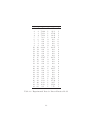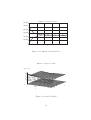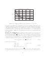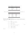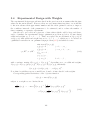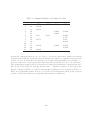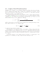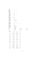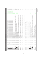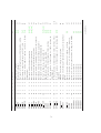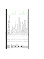
1
Data Fitting and Experimental Design in Dynamical Systems with - User’s Guide - Prof. K. Schittkowski Department of Computer Science University of Bayreuth Version 5.1, 2009 c Copyright 1997-2009, Klaus Schittkowski June 24, 2009 EASY-FITM odelDesign is an interactive software system to identify parameters in explicit model functions, dynamical systems of equations, Laplace transformations, systems of ordinary differential equations, differential algebraic equations, or systems of one-dimensional time-dependent partial differential equations with or without algebraic equations. Proceeding from given experimental data, i.e., observation times and measurements, the minimum least squares distance of measured data from a fitting criterion is computed, that depends on the solution of the dynamical system. Moreover, it is possible to predetermine an optimal experimental design by fixing the model parameters. Additional design parameters, for example initial concentrations or input feeds, are used to minimize the size of confidence intervals. Weight optimization helps to identify relevant time values where experiments can be taken. The mathematical background of the numerical algorithms is described in Schittkowski [438] in form of a comprehensive textbook. Also, the outcome of numerical comparative performance evaluations is found there, together with a chapter about numerical pitfalls, testing the validity of models, and a collection of 12 real-life case studies. Most of the case studies possess an industrial background. The software system is implemented in form of a database under Microsoft Office Access 2007 running under Windows XP or higher, and comes with the royalty-free runtime version. The underlying numerical algorithms are coded in Fortran and are executable independently from the interface. Model functions are either interpreted and evaluated symbolically by a program called PCOMP permitting automatic differentiation of nonlinear model functions, or by user-provided Fortran subroutines. In the latter case, interfaces for the Fortran compilers Watcom F77/386, Salford FTN77, Lahey F77L-EM/32, Compaq Visual Fortran, Absoft Pro Fortran, Microsoft Fortran PowerStation, and Intel Visual Fortran for Windows 32 and Windows 64 environments are provided. Important Notes: 1. Trademarks: Windows, Microsoft, PowerStation are registered trademarks of Microsoft Corp. WATCOM is a registered trademark of WATCOM Systems Inc. FTN77 is a trademark of Salford Software Ltd. INTEL is a trademark of Intel Corporation Adobe, Acrobat are registered trademarks of Adobe Systems Inc. 2. Copyrights: c GNUPLOT Copyright 1986-1993,1998,2004, Thomas Williams, Colin Kelley c RADAU5, DOPRI5 Copyright 2004, Ernst Hairer c LAPACK Copyright 1992-2007, The University of Tennessee 3. Data Fitting Codes: Note that with Version 4.32 of EASY-FITM odelDesign the data fitting algorithm DFNLP has been replaced by the codes NLPLSQ - least squares data fitting NLPLSX - least squares data fitting for very many measurements NLPL1 - L1 data fitting (sum of absolute residual values) NLPINF - L∞ data fitting (maximum of absolute residual values) Disclaimer: THIS SOFTWARE IS PROVIDED BY THE COPYRIGHT HOLDERS AND CONTRIBUTORS ’AS IS’ AND ANY EXPRESS OR IMPLIED WARRANTIES, INCLUDING, BUT NOT LIMITED TO, THE IMPLIED WARRANTIES OF MERCHANTABILITY AND FITNESS FOR A PARTICULAR PURPOSE ARE DISCLAIMED. IN NO EVENT SHALL THE REGENTS OR CONTRIBUTORS BE LIABLE FOR ANY DIRECT, INDIRECT, INCIDENTAL, SPECIAL, EXEMPLARY, OR CONSEQUENTIAL DAMAGES (INCLUDING, BUT NOT LIMITED TO, PROCUREMENT OF SUBSTITUTE GOODS OR SERVICES; LOSS OF USE, DATA, OR PROFITS; OR BUSINESS INTERRUPTION) HOWEVER CAUSED AND ON ANY THEORY OF LIABILITY, WHETHER IN CONTRACT, STRICT LIABILITY, OR TORT (INCLUDING NEGLIGENCE OR OTHERWISE) ARISING IN ANY WAY OUT OF THE USE OF THIS SOFTWARE, EVEN IF ADVISED OF THE POSSIBILITY OF SUCH DAMAGE. Contents 0.1 Installation . . . . . . . . . . . . . . . . . . 0.1.1 Hardware and Software Requirements 0.1.2 Packing List . . . . . . . . . . . . . . 0.1.3 System Setup . . . . . . . . . . . . . 0.1.4 Starting EASY-FITM odelDesign . . . 0.1.5 Dimensioning Parameters . . . . . . . . . . . . . . . . . . . . . . . . . . . . . . . . . . . . . . . . . . . . . . . . . . . . . . . . . . . . . . . . . . . . . . . . . . . . . . . . . . . . . . . . . . . . . . . . . . . . . . . . . . . . . . . . . . 1 Introduction i i i iii v vi 1 2 Data Fitting Models 2.1 Introduction . . . . . . . . . . . . . . . . . . . . . . . . . . 2.2 Explicit Model Functions . . . . . . . . . . . . . . . . . . . 2.3 Laplace Transforms . . . . . . . . . . . . . . . . . . . . . . 2.4 Steady State Equations . . . . . . . . . . . . . . . . . . . . 2.5 Ordinary Differential Equations . . . . . . . . . . . . . . . 2.5.1 Standard Formulation . . . . . . . . . . . . . . . . 2.5.2 Differential Algebraic Equations . . . . . . . . . . . 2.5.3 Switching Points . . . . . . . . . . . . . . . . . . . 2.5.4 Constraints . . . . . . . . . . . . . . . . . . . . . . 2.5.5 Shooting Method . . . . . . . . . . . . . . . . . . . 2.5.6 Boundary Value Problems . . . . . . . . . . . . . . 2.5.7 Variable Initial Times . . . . . . . . . . . . . . . . 2.6 Partial Differential Equations . . . . . . . . . . . . . . . . 2.6.1 Standard Formulation . . . . . . . . . . . . . . . . 2.6.2 Partial Differential Algebraic Equations . . . . . . . 2.6.3 Flux Functions . . . . . . . . . . . . . . . . . . . . 2.6.4 Coupled Ordinary Differential Algebraic Equations 2.6.5 Integration Areas and Transition Conditions . . . . 2.6.6 Switching Points . . . . . . . . . . . . . . . . . . . 2.6.7 Constraints . . . . . . . . . . . . . . . . . . . . . . 2.7 Optimal Control Problems . . . . . . . . . . . . . . . . . . 4 . . . . . . . . . . . . . . . . . . . . . . . . . . . . . . . . . . . . . . . . . . . . . . . . . . . . . . . . . . . . . . . . . . . . . . . . . . . . . . . . . . . . . . . . . . . . . . . . . . . . . . . . . . . . . . . . . . . . . . . . . . . . . . . . . . . . . . . . . . . . . . . . . . . . . . . . . . . . . . . . . . . . . . . . . . . . . . . . . . . . . . . . . . . . . . . . . . . . . . . . . . . . . . . . . . 1 2 4 9 11 14 14 15 17 26 28 35 37 43 43 45 48 50 56 61 65 71 3 Statistical Analysis and Experimental Design 3.1 Confidence Intervals . . . . . . . . . . . . . . 3.2 Significance Levels . . . . . . . . . . . . . . . 3.3 Experimental Design . . . . . . . . . . . . . . 3.4 Experimental Design with Weights . . . . . . . . . . 79 81 83 89 101 . . . . . . . . 1 1 2 3 4 5 6 9 10 Modeling Language PCOMP Automatic Differentiation . . . . . . . . . . . . . . . . . . . . . . . . . . . . Input Format for PCOMP . . . . . . . . . . . . . . . . . . . . . . . . . . . . Error Messages of PCOMP . . . . . . . . . . . . . . . . . . . . . . . . . . . . 1 1 4 15 4 Numerical Algorithms 4.1 Data Fitting Algorithms . . . . . . . . 4.2 Steady State Systems . . . . . . . . . . 4.3 Laplace Back-Transformation . . . . . 4.4 Ordinary Differential Equations . . . . 4.5 Differential Algebraic Equations . . . . 4.6 Partial Differential Equations . . . . . 4.7 Partial Differential Algebraic Equations 4.8 Statistical Analysis . . . . . . . . . . . 5 The 5.1 5.2 5.3 . . . . . . . . . . . . . . . . . . . . . . . . . . . . . . . . . . . . . . . . . . . . . . . . . . . . . . . . . . . . . . . . . . . . . . . . . . . . . . . . . . . . . . . . . . . . . . . . . . . . . . . . . . . . . . . . . . . . . . . . . . . . . . . . . . . . . . . . . . . . . . . . . . . . . . . . . . . . . . . . . . . . . . . . . . . . . . . . . . . . . . . . . . . . . . . . . . . . . . . . . . . . . . . . . . . . . . . . . . . . . . . . 6 Model Functions and Equations 6.1 Explicit Model Functions . . . . . . . . . . . . 6.2 Laplace Transformations . . . . . . . . . . . . 6.3 Systems of Steady State Equations . . . . . . 6.4 Ordinary Differential Equations . . . . . . . . 6.5 Differential Algebraic Equations . . . . . . . . 6.6 Time-Dependent Partial Differential Equations 6.7 Partial Differential Algebraic Equations . . . . . . . . . . . . . . . . . . . . . . . . . . . . . . . . . . . . . . . . . . . . . . . . . . . . . . . . . . . . . . . . . . . . . . . . . . . . . . . . . . . . . . . . . . . . . . . . . . . . . . . . . . . . . . . . . . . . . . . . . . . 1 1 3 4 6 8 10 13 7 Problem Data and Solution Tolerances 7.1 Model Independent Information . . . . 7.1.1 Problem Name . . . . . . . . . 7.1.2 Documentation Text . . . . . . 7.1.3 Parameters to be Estimated . . 7.1.4 Input Type of Model Functions 7.1.5 Numerical Analysis . . . . . . . 7.1.6 Optimization Tolerances . . . . 7.1.7 Scaling . . . . . . . . . . . . . . 7.1.8 Number of Plot Points . . . . . 7.1.9 Logarithmic Plot . . . . . . . . 7.1.10 Experimental Data . . . . . . . . . . . . . . . . . . . . . . . . . . . . . . . . . . . . . . . . . . . . . . . . . . . . . . . . . . . . . . . . . . . . . . . . . . . . . . . . . . . . . . . . . . . . . . . . . . . . . . . . . . . . . . . . . . . . . . . . . . . . . . . . . . . . . . . . . . . . . . . . . . . . . . . . . . . . . . . . . . . . . . . . . . . . . . . . . . . . . . . . . . . . . . . . . . 1 1 1 2 3 3 4 6 11 11 11 11 . . . . . . . . . . . . . . . . . . . . . . . . . . . . . . . . . . . . . . . . . . . . . . . . . . . . . 12 13 13 16 20 21 26 33 40 . . . . . . . . 1 1 5 6 7 10 14 15 16 9 External Usage of Numerical Codes 9.1 MODFIT: Explicit Model Functions, Dynamical Systems, ODE’s and DAE’s 9.2 PDEFIT: Partial Differential Equations . . . . . . . . . . . . . . . . . . . . . 1 1 28 10 Test Examples 10.1 Explicit Model Functions . . . . . . . . 10.2 Laplace Transforms . . . . . . . . . . . 10.3 Steady State Equations . . . . . . . . . 10.4 Ordinary Differential Equations . . . . 10.5 Differential Algebraic Equations . . . . 10.6 Partial Differential Equations . . . . . 10.7 Partial Differential Algebraic Equations 1 3 14 15 18 41 45 60 7.2 7.1.11 Model 7.2.1 7.2.2 7.2.3 7.2.4 7.2.5 7.2.6 7.2.7 Data Fitting Norm . . . . . . . . . . . . . . . . . . . . . . . . Dependent Information . . . . . . . . . . . . . . . . . . . . . . Model Data for Explicit Functions . . . . . . . . . . . . . . . . Model Data for Steady State Equations . . . . . . . . . . . . . Model Data for Laplace Transformations . . . . . . . . . . . . Model Data for Ordinary Differential Equations . . . . . . . . Model Data for Differential Algebraic Equations . . . . . . . . Model Data for Time-Dependent Partial Differential Equations Model Data for PDAE’s . . . . . . . . . . . . . . . . . . . . . 8 Menu Commands 8.1 File Command . . 8.2 Edit Command . . 8.3 Start Command . . 8.4 Report Command . 8.5 Data Command . . 8.6 Delete Command . 8.7 Make Command . . 8.8 Utilities Command . . . . . . . . . . . . . . . . . . . . . . . . . . . . . . . . . . . . . . . . . . . . . . . . . . . . . . . . . . . . . . . . . . . . . . . . . . . . . . . . . . . . . . . . . . . . . . . . . . . . . . . . . . . . . . . . . . . . . . . . . . . . . . . . . . . . . . . . . . . . . . . . . . . . . . . . . . . . . . . . . . . . . . . . . . . . . . . . . . . . . . . . . . . . . . . . . . . . . . . . . . . . . . . . . . . . . . . . . . . . . . . . . . . . . . . . . . . . . . . . . . . . . . . . . . . . . . . . . . . . . . . . . . . . . . . . . . . . . . . . . . . . . . . . . . . . . . . . . . . . . . . . . . . . . . . . . . . . . . . . . . . . . . . . . . . . . . . . . . . . . . . . . . . . . . . . . . . . . . . . . . . . . . . . . . . . . . . . . . . . . . . . . . . . . . . . . . . . . . . . . . . . . . . . . . . . . . . . . . . . . . 0.1 Installation EASY-FITM odelDesign consists of a database containing models, data and results, and of underlying numerical algorithms for solving the parameter estimation problem depending on the mathematical structure, i.e. MODFIT parameter estimation in explicit functions, steady state equations, Laplace transforms, ordinary differential and differential algebraic equations PDEFIT parameter estimation in one-dimensional time-dependent partial differential equations and partial differential algebraic equations By the following notes, the system installation and hardware requirements are outlined. 0.1.1 Hardware and Software Requirements Installation of EASY-FITM odelDesign requires 95 MB on hard disk plus 130 MP for the Microsoft Office Access 2007 runtime version. The program runs under Windows XP or higher. EASY-FITM odelDesign comes with the royalty-free runtime version of Microsoft Office Access 2007 (English). All model functions are defined in the PCOMP modelling language to be interpreted and evaluated during run time. Derivatives, as far as needed, are computed by automatic differentiation. The full version of EASY-FITM odelDesign allows also the most flexible input of the underlying model functions in form of Fortran code, and has interfaces for Compaq Visual Fortran, Watcom F77/386, Salford FTN77, Lahey F77L-EM/32, Absoft Pro Fortran, Microsoft Fortran PowerStation, and Intel Visual Fortran for Windows 32 and Windows 64 environments, where the compiler and linker options can be altered and adapted interactively. 0.1.2 Packing List Basically, EASY-FITM odelDesign consists of a user interface in form of a database implemented in Microsoft Office Access 2007, and some numerical routines. The following essential files and directories are submitted: i Numerical codes: MODFIT.EXE Solving parameter estimation problems in explicit models, time-dependent algebraic equations, ordinary differential equations, differential algebraic systems, and Laplace transforms MODFIT.FOR Corresponding Fortran source code (only complete version) MODFUN E.FOR Frame of a Fortran code for estimating parameters in explicit model functions MODFUN O.FOR Frame of a Fortran code for estimating parameters in differential equations MODFUN A.FOR Frame of a Fortran code for estimating parameters in differential algebraic equations MODFUN S.FOR Frame of a Fortran code for estimating parameters in steady state systems MODFIT.INC Include file with dimensioning parameters for MODFIT PDEFIT.EXE Solving parameter estimation problems in systems of one-dimensional partial differential equations and partial differential algebraic equations PDEFIT.FOR Corresponding Fortran source code (only complete version) PDEFUN.FOR Frame of a Fortran code for estimating parameters in systems of partial differential equations PDEFIT.INC Include file with dimensioning parameters for PDEFIT COMPILE.BAT DOS batch file to execute the Fortran compiler, can be modified interactively LINKER.BAT DOS batch file to execute the Fortran linker, can be modified interactively ii Plot programs and editor: SP PLOT.EXE Standard plot program, where input data are read from files GNUPLOT.EXE Public domain plot program Gnuplot EDITOR.EXE Syntax-highlighting external editor Database: EASY FIT.MDE EASY FIT.HLP EASY FIT.ICO EASY FIT.PDF Main database of EASY-FITM odelDesign containing tables, forms, reports, macros and modules Corresponding help file Icon file for EASY-FITM odelDesign Adobe Acrobat Reader file containing complete documentation Subdirectories: OBJECT PROBLEMS < ∗ >.FUN and < ∗ >.FOR 0.1.3 Directory with object codes for the Watcom, Salford, Lahey, Compaq, Absoft, Microsoft, and Intel Fortran compilers containing underlying optimization algorithms and ODE/PDE-solvers (only complete version) Directory for test example files with extensions System Setup Download the file EASYFIT.EXE and start the installation by clicking on this file. In case of a local network, administrator rights are required. If there exists an older version of EASYFITM odelDesign , it is recommended to save first all problems of interest to a temporary directory. After successful installation, the saved problems can be imported again. EASYFITM odelDesign comes with the royalty-free runtime version of Microsoft Office Access 2007. When starting EASY-FITM odelDesign the first time after a successful setup, a couple of directory strings are inserted automatically into an internal table. They can be adapted to a special situation depending on the environment given. Alterations can be made by the Utilities command in the menu bar. E.g., the favorite text editor may be defined to be used for input and modification of model functions. In more detail, the following configuration information is available: iii Figure 1: Configuration Form iv Name system directory Default C:\EASYFIT\ editor [EASY-FIT] graphics system [EASY-FIT] Fortran compiler SALFORD Contents main directory with database, help files etc. Internal or alternative external editor, for example EDITOR.EXE Internal or alternative external graphics system identified by string GNUPLOT Available Fortran compiler. Insert ABSOFT, WATCOM, SALFORD, LAHEY, V FORTRAN, MS POWER, INTEL, or INTEL64 for Absoft Pro Fortran, Watcom F77/386, Salford FTN77, Lahey F77LEM/32, Compaq Visual Fortran, Microsoft Fortran PowerStation, Intel Visual Fortran compiler (IA32) and Intel Visual Fortran 64 bit compiler (EM64T), respectively EASY-FITM odelDesign In case of installing an EASY-FITM odelDesign version coming with all object files, proceed as follows. First, the submitted object codes of the numerical algorithms must be copied to a subdirectory with name OBJECT. The object codes of the driving routines with names MODFIT*.FOR and PDEFIT*.FOR can be generated subsequently, if necessary. The easiest way is to edit dimensioning parameters in the Utilities menu and to let these modules be compiled automatically by EASY-FITM odelDesign . If the submitted default compiler interface is to be changed, e.g., from the Watcom to the Salford or Lahey compiler, the user has to set corresponding compiler name, some path names, and the compiler and linker execution commands. An external editor can used to create or modify model functions either in the PCOMP or the Fortran language. Note that EASY-FITM odelDesign is delivered with two editors, an internal GUI form ([EASY-FIT]) and an external executable one with syntax highlighting (EDITOR.EXE). Both allow direct parse of PCOMP code or compilation and link of Fortran code. To use the external editor, the file EDITOR.EXE must be part of the EASYFITM odelDesign installation directory. 0.1.4 Starting EASY-FITM odelDesign It is recommended to start EASY-FITM odelDesign always from its shortcut in the program menu generated by the setup program, or from a corresponding desktop icon to avoid conflicts with an existing Microsoft Office Access version. The welcome window of EASYFITM odelDesign is displayed and the main form of the database is opened. If the main form cannot be opened correctly, please check the language settings. Nonunicode languages like Chinese, Arabic or other settings cause some problems. If the database reacts too slow, for example when starting a data fitting code or when displaying a report, delete a certain subset of problems you do not need. v The file README.TXT contains last-minute changes, a summary of new features and especially the information how to transfer parameter estimation problems from easier versions of EASY-FITM odelDesign to the new one. Figure 2: Welcome Form If something goes wrong, please contact the author under phone fax e-mail home page 0.1.5 : +49 (0)921 553278 : +49 (0)921 35557 : [email protected] : http://www.klaus-schittkowski.de Dimensioning Parameters The numerical algorithms require dimensioning parameters for defining working arrays of suitable lengths. They serve also as upper bounds for certain model parameters, i.e., maximum number of variables to be estimated or maximum number of measurements. Whereas the full version can be adapted to any size, there are some restrictions for the demo version: vi Number Number Number Number Number Number Number of of of of of of of parameters to be estimated: equations: constraints: ODEs of discretized PDE: time values: measurement sets: measurements: 2 2 5 100 20 2 40 To find out the allowed maximum problem sizes of the full version, one should investigate the corresponding include files MODFIT.INC and PDEFIT.INC from the utilities command of the menu bar. New executable files can be linked subsequently, if any of the bounds are changed, and if object codes are available. The meaning of the parameters used is completely described by initial comments. vii Chapter 1 Introduction Parameter estimation plays an important role in natural science, engineering, and many other disciplines. The key idea is to estimate unknown parameters p1 , . . ., pn of a mathematical model that describes a real life situation, by minimizing the distance of some known experimental data from theoretically predicted values of a model function at certain time values. Thus, also model parameters that cannot be measured directly, can be identified by a least squares fit and analyzed subsequently in a quantitative way. In mathematical and somewhat simplified notation, we want to solve a least squares problem of the form p ∈ IR : n min l i=1 (h(p, y(p, ti), ti ) − yi )2 pl ≤ p ≤ pu , (1.1) where h(p, y, t) is a fitting function depending on the unknown parameter vector p, the time t, and the solution y(p, t) of an underlying dynamical system. A typical dynamical system is given by differential equations that describe a time-dependent process, and that depend on the parameter vector p. Instead of minimizing the sum of squares, we may apply alternative residual norms, for example with the goal to minimize the sum of absolute residual values or the maximum of absolute residual values. Parameter estimation, also called parameter identification, nonlinear regression, or data fitting, is extremely important in all practical situations, where a mathematical model and corresponding experimental data are available to analyze the behavior of a dynamical system. The main goal of the documentation is to introduce some numerical methods that can be used to compute parameters by a least squares fit in form of a toolbox. The mathematical model that is set up by a system analyst, has to belong to one of the following categories, • explicit model functions, • steady state systems, • Laplace transforms of differential equations, 1 • ordinary differential equations, • differential algebraic equations, • one-dimensional time-dependent partial differential equations, • one-dimensional partial differential algebraic equations. To understand at least some of the basic features of the presented algorithms, to apply available software, and to analyze numerical results, it is necessary to combine knowledge from many different mathematical disciplines, for example - modelling, - nonlinear optimization, - system identification, - numerical solution of ordinary differential equations, - discretization of partial differential equations, - sensitivity analysis, - automatic differentiation, - Laplace transforms, - statistics. The mathematical background of the numerical algorithms is described in Schittkowski [438] in form of a comprehensive textbook. Also, the outcome of numerical comparative performance evaluations is found there, together with a chapter about numerical pitfalls, testing the validity of models, and a collection of 12 real-life case studies. Most of the case studies possess an industrial background. The general mathematical model to be investigated contains certain features to apply the numerical methods to a large set of practically relevant situations. Some of the most important issues are: 1. More than one fitting criterion can be defined, i.e., more than one experimental data set can be fitted within a model formulation. 2. The fitting criteria are arbitrary functions depending on the parameters to be estimated, the solution of the underlying dynamical system, and the time variable. 3. The model may possess arbitrary equality or inequality constraints with respect to the parameters to be estimated, and upper and lower bounds for the parameters. 2 4. Model equations may contain an additional independent parameter, for example experimental concentration or temperature values. 5. Differential-algebraic equations can be solved up to index 3. Consistent initial values for index-1-formulations are computed internally. 6. In case of partial differential equations, also coupled ordinary differential equations and non-continuous transitions for state variable and flux between different areas can be taken into account. 7. Differential equation models may possess additional break or switching points, where the model dynamics is changed and where integration is restarted, for example if a new dose is applied in case of a pharmacokinetic model. 8. The switching points mentioned before, may become optimization variables to allow the modeling of dynamical input, for instance, to compute optimal bang-bang feed controls of a chemical reactor. 9. The model functions may be defined by their Laplace transforms, where the backtransformation is performed numerically. 10. Gradients can be evaluated by automatic differentiation without additional round-off, truncation or approximation errors, and without compiling and linking of code. 11. Ordinary differential equations may become stiff and large. We introduce explicit and implicit methods and exploit band structures. 12. Parameter estimation problems based on unstable differential equations can be solved by the shooting method. 13. Various types of one-dimensional partial differential equations are permitted, also hyperbolic ones describing shock waves. Advection, diffusion, transport, or related equations can be solved successfully by non-oscillatory discretization schemes, even with non-continuous initial or boundary conditions. 14. Partial differential equations may be defined with Neumann and Dirichlet boundary or transitions conditions. Moreover, these conditions can be formulated in terms of algebraic equations coupled at arbitrary spatial positions. 15. Algebraic partial differential equations may be added to the time-dependent ones. 16. Data can be fitted with respect to the L2 -, the L1 -, or the L∞ -norm, i.e., with respect to sum of squares, sum of absolute values, or maximum of absolute values of the residuals. 3 17. A statistical analysis provides confidence intervals for parameters depending on an userprovided estimate for the variance. Moreover, correlation coefficients and covariance matrix are computed. 18. Proceeding from the inverse of the Fisher information matrix, an eigenvalue/eigenvector analysis is performed to identify significant parameter levels for subsequent elimination of non-relevant parameters or further statistical design investigations. Only for illustration purposes we denote the first independent model variable the time variable of the system, the second one the concentration variable and the dependent data as measurement values of an experiment. These words describe their probably most frequent usage in a practical situation. On the other hand, the terms may get any other meaning depending on the underlying application problem. Due to the practical importance of parameter estimation, very many numerical codes have been developed in the past and are distributed within software packages. However, there is no guarantee that a mathematical algorithm is capable to solve the problem we are interested in. Possible traps preventing a solution in the desired way, are • approximation of a local solution that is unacceptable, • round-off errors because of an inaccurate iterative solution of the dynamical system, • narrow curved valleys where progress towards the solution is hard to achieve, • very flat objective function in the neighborhood of a solution, for example, when there are large perturbations in measurement data, • overdetermined models in case of too many model parameters to be estimated, leading to infinitely many solution vectors, • bad starting values for parameters requiring a large number of steps, • badly scaled model functions and, in particular, measurement values, • non-differentiable model functions. We have to know that all efficient optimization algorithms developed for the problem class we are considering, require differentiable fitting criteria and the availability of a starting point from which the iteration cycle is initiated. Additional difficulties arise in the presence of nonlinear constraints, in particular if they are badly stated, ill-conditioned, badly scaled, linearly dependent, or, worst of all, contradictory. Thus, users of parameter estimation software are often faced with the situation that the algorithm is unable to get a satisfactory return subject to the given solution tolerances, and that one has to restart the solution cycle by changing tolerances, internal algorithmic 4 decisions, or at least the starting values to get a better result. To sum up, a black box approach to solve a parameter estimation problem does not exist and a typical life cycle of a solution process consists of stepwise redesign of solution data. The parameter estimation problem, alternative phrases are data fitting or system identification, is outlined in Chapter 2. Is is shown, how the dynamical systems have to be adapted to fit into the least squares formulation required for starting an optimization algorithm. A first question is always how to get suitable confidence intervals for the estimated parameters. This is one of the main investigations when analyzing the output of data fitting. Related problems are whether it is possible at all to identify parameters, or how to eliminate redundant ones, as will be discussed in the subsequent sections. Another important question is experimental design, where we want to create or improve existing experimental conditions. The goals are to reduce the number of costly experiments, to reduce error variances, or to get identifiable parameters. The corresponding tools are summarized in Chapter 3. A brief review of the numerical algorithms implemented, is presented in Chapter 4. Only some basic features of the underlying ideas are presented. More details are found in the references and in particular in Schittkowski [438]. The codes allow the numerical identification of parameters in any of the six situations under investigation. The executable files are called MODFIT.EXE and PDEFIT.EXE. Nonlinear model functions can be evaluated symbolically. Thus, any compilation and link of Fortran subroutines is not required whenever model functions are defined or altered in this way. A particular advantage of this approach is the automatic differentiation of model functions to avoid numerical truncation errors. The corresponding program is called PCOMP, see Dobmann, Liepelt and Schittkowski [115], and is part of the executable codes. The automatic differentiation algorithm, the PCOMP language and error messages of the parser are described in Chapter 5. Model functions must be provided by the user either in form of the PCOMP language mentioned above, or in form of Fortran code. In the latter case, the preparation of function and gradient values is described by initial comments of a code inserted by EASYFITM odelDesign as a frame. In case of PCOMP input, the order in which variables and functions are to be inserted, identifies their role in the mathematical model. A full documentation of the model function input in this situation is presented in Chapter 6. The interactive system EASY-FITM odelDesign proceeds from a database for storing model information, experimental data and results. A complete context sensitive help option is included containing additional technical and organizational information about the input of data and optimization tolerances, for example. A brief outline of data organization and input is found in Chapter 7. The corresponding menu commands to define or alter data and functions, to start an optimization run or to get reports on numerical results, are described in Chapter 8. The numerical parameter estimation codes MODFIT and PDEFIT can be executed also outside of the interactive user interface. A possible reason could be the solution of a large number of parameter estimation problems controlled by a separate command shell. In this 5 case, a data input file is required that contains all information for starting the numerical algorithm. The format of this file is documented in Chapter 9 in detail. Usage of the codes is illustrated by a few test examples. The database of the delivered EASY-FITM odelDesign version contains 1,300 academic and real life examples, i.e., test problems with some realistic practical background. Application areas are pharmacy, biochemistry, chemical engineering, and mechanical engineering. The purpose for attaching a comprehensive collection of test problems in Chapter 10, is to become familiar with the PCOMP language and the implementation of a new model, since a large variety of different model structures is offered. The problems can be used for selecting a reference example when trying to install own dynamical models, or to test the accuracy or efficiency of the algorithms available within EASY-FITM odelDesign . 6 Chapter 2 Data Fitting Models Our goal is to estimate parameters in • explicit model functions, • Laplace transforms, • steady state systems, • systems of ordinary differential equations • systems of differential algebraic equations, • systems of one-dimensional, time-dependent partial differential equations, • systems of one-dimensional partial differential algebraic equations. Proceeding from given experimental data, i.e., observation times and measurements, the minimum least squares distance of measured data from a fitting criterion is to be computed that depends on the solution of the dynamical system. In this chapter, we summarize in detail, how the model functions fi (p) depend on the solution of a dynamical system. Moreover, we describe a couple of extensions of the data fitting problem and the dynamical system to be able to treat also more complex practical models. Most examples contain the name of the corresponding test problem of the EASY-FITM odelDesign database, from where implementation details and further data can be retrieved, in some cases only in modified form. 1 2.1 Introduction The basic mathematical model is the least squares problem to minimize a sum of squares of nonlinear functions of the form p ∈ IR : n min l i=1 fi (p)2 pl ≤ p ≤ pu (2.1) . Here, we assume that the parameter vector p is n-dimensional and that all nonlinear functions are continuously differentiable with respect to p. Upper and lower bounds are included to restrict the search area. fi (p) is a suitable fitting criterion which may depend on the solution of an underlying dynamical system, e.g., a system of ordinary differential equations. Alternatively the L2 -norm may be changed to another one, e.g., to minimize the maximum distance of experimental data from a model function. Thus, we formulate either the L1 -problem min li=1 |fi (p)| n p ∈ IR : (2.2) pl ≤ p ≤ pu or the L∞ -problem p ∈ IRn : min maxi=1,...,l |fi (p)| pl ≤ p ≤ pu . (2.3) However, we assume that our models a dynamic, i.e., depend on an additional parameter, in most cases the time. In addition, there might be an additional independent model parameter by which, e.g., a concentration or temperature value is to be specified from where a set of measurements is obtained. To illustrate the situation, we omit possible additional data sets, dependencies on underlying dynamical systems, and constraints on the parameters, and differ between three situations. 1. Time-dependent models: The model function fi (p) depends on the experimental time, i.e., we have measurements of the form (ti , yi ) , i = 1, . . . , l , (2.4) moreover a model function h(p, t), and we want to estimate the parameter vector p by minimizing l 2 min i=1 (h(p, ti ) − yi ) n p ∈ IR : (2.5) pl ≤ p ≤ pu . In this case, we define fi (p) = h(p, ti ) − yi, i = 1, . . . , l . 2 (2.6) 2. Time- and concentration dependent fitting criteria: The data fitting function fi (p) depends on the experimental time and an additional parameter which we call concentration. Any other physical meaning is, of course, allowed. We proceed from measurements of the form (ti , ci , yi ) , i = 1, . . . , l , (2.7) a model function h(p, t, c), and we want to estimate the parameter vector p by minimizing min li=1 (h(p, ti , ci ) − yi )2 n (2.8) p ∈ IR : pl ≤ p ≤ pu . In this case, we define fi (p) = h(p, ti , ci ) − yi , i = 1, . . . , l . (2.9) Advantages are the possibilities to define a model as a function of t and c, and to generate three-dimensional plots. The drawback of this formulation, however, is that an underlying differential equation cannot depend on c as well, since we would have to evaluate the right-hand side of an equation also at intermediate times and would not know how to insert a suitable concentration value. 3. Time- and concentration dependent models: To overcome the drawback mentioned above, we assume that the dynamical model, say an ordinary differential equation, depends on an additional, in the statistical sense independent parameter c, i.e., c may be inserted into initial values, right-hand sides, fitting criterion, or even constraints. Now we proceed from measurements of the form (ti , cj , yij ) , i = 1, . . . , lt , j = 1, . . . , lc . (2.10) The model function is again given in the form h(p, t, c), and we want to estimate the parameter vector p by minimizing p ∈ IR : n min lt i=1 lc j=1 pl ≤ p ≤ pu (h(p, ti , cj ) − yij )2 . (2.11) Now we get the fitting criterion fij (p) = h(p, ti , cj ) − yij , i = 1, . . . , lt ; , j = 1, . . . , lc . (2.12) In the subsequent sections, we proceed from the most general situation (2.11) and illustrate our approaches by examples. 3 2.2 Explicit Model Functions In this section, we restrict our investigations to parameter estimation problems, where one vector-valued model function is available in explicit form, the so-called fitting criterion, with one additional variable called time, and optionally with another one called concentration. We proceed now from r measurement sets, given in the form (ti , cj , yijk ) , i = 1, . . . , lt , j = 1, . . . , lc , k = 1, . . . , r , (2.13) where lt time values, lc concentration values and l = lt lc r corresponding measurement values are defined. Together with a vector-valued model function h(p, t, c) = (h1 (p, t, c), . . . , hr (p, t, c))T , we get a data fitting formulation (2.1), (2.2), or (2.3), by fs (p) = wijk (hk (p, ti , cj ) − yijk ) , (2.14) where s runs from 1 to l = lt lc r in any order. Moreover, we assume that there are suitable weight factors wijk ≥ 0 given by the user that are to reflect the individual influence of a measurement on the whole experiment. Zero weights can be defined, if, for example, there are several concentration values c1 , . . ., clc , but measurements are not available for each time value t1 , . . ., tlt . The basic idea is to minimize the distance between the model function at certain time and concentration points and the corresponding measurement values. This distance is denoted as the residual of the problem. In the ideal case, the residuals are zero indicating a perfect fit of the model function by the measurements. In addition, we allow any nonlinear restrictions on the parameters to be estimated, in form of general equality or inequality constraints gj (p) = 0, j = 1, ..., me , gj (p) ≥ 0, j = me + 1, ..., mr . (2.15) It must be assumed that all constraint functions are continuously differentiable with respect to p. To summarize, the resulting least squares problem is of the form min p ∈ IRn : r k=1 lt i=1 lc j=1 (wijk (hk (p, ti , cj ) − yijk ))2 gj (p) = 0 , j = 1, ..., me , gj (p) ≥ 0 , j = me + 1, ..., mr , pl ≤ p ≤ pu , 4 (2.16) see (2.1). Alternatively we get the corresponding L1 -formulation by minimizing r lc lt wijk |hk (p, ti , cj ) − yijk | , k=1 i=1 j=1 see (2.2), or the L∞ -formulation max k=1,...,r;i=1,...,lt ;j=1,...,lc wijk |hk (p, ti , cj ) − yijk | , see (2.3). Example 2.1 (RAT APP) We want to fit some parameters p1 , . . ., p4 , so that the data of Table 2.1 are approximated by a rational function h(p, t) = p1 t2 + p2 t , t2 + p3 t + p4 see Lindstr¨om [288] and Deuflhard, Apostolescu [112]. There is no concentration parameter, but we want to fit the outer measurement values exactly, i.e., we define two additional nonlinear equality constraints g1 (p) = h(p, t1 ) − y1 and g2 (p) = h(p, tl ) − yl with l = 11. There is only one measurement set and all weights are set to 1. Thus, the least squares data fitting problem is l 2 min i=1 (h(p, ti ) − yi ) p ∈ IR4 : g1 (p) = 0 , g2 (p) = 0 . When starting the code DFNLP of Schittkowski [429] from p0 = (0.25, 0.39, 0.415, 0.39)T with a termination tolerance of 10−12 , we get the solution vector p = (0.1923, 0.4040, 0.2750, 0.2068)T after 10 iterations. The final residual is 3.78 · 10−3 and the maximum constraint violation is 3.1 · 10−13 . The individual residuals and the relative errors are also listed in Table 2.1. Model function and data are plotted in Figure 2.1. Since the model function h(p, t, c) does not depend on the solution of an additional dynamical system, we call it an explicit model function. Otherwise, h(p, t, c) may depend on the solution vector y(p, t, c) of an auxiliary problem, for example an ordinary differential equation that is implicitly defined. Models of this kind are considered in the subsequent sections. But explicit model functions can reflect solutions of dynamical systems, that are analytically solvable, as shown by the subsequent example. 5 ti 0.0625 0.0714 0.0823 0.1 0.125 0.167 0.25 0.5 1.0 2.0 4.0 |h(p , ti ) − yi | 2.5230 · 10−14 4.6890 · 10−3 2.7982 · 10−4 5.4681 · 10−3 3.9113 · 10−3 2.6394 · 10−3 8.5962 · 10−3 1.3765 · 10−2 8.6748 · 10−3 3.6381 · 10−4 8.0491 · 10−16 yi 0.0246 0.0235 0.0323 0.0342 0.0456 0.0627 0.0844 0.16 0.1735 0.1947 0.1957 error 0.0 % 20.0 % 0.9 % 16.0 % 8.6 % 4.2 % 10.2 % 8.6 % 5.0 % 0.2 % 0.0 % Table 2.1: Experimental Data and Final Residuals Rational Approximation 0.2 2 2 0.18 2 0.16 2 0.14 h(p, t) 0.12 0.1 2 0.06 2 2 0.04 2 0.02 2 0.08 0 0.5 1 1.5 2 t 2.5 3 Figure 2.1: Function and Data Plot 6 3.5 4 Linear Compartmental Model h1 (p, t, c) 150 100 50 0 150 0 100 20 40 50 60 t c 50 Figure 2.2: Function and Data Plot Example 2.2 (LKIN X3) The next test case consists of an explicit solution of a linear ordinary differential equation h1 (p, t, c) = c exp(−p1 t) , 1c h2 (p, t, c) = p p− p2 (exp(−p2 t) − exp(−p1 t)) . 1 The concentration parameter represents now the initial dose of an experiment, and is set to c1 = 50, c2 = 100, and c3 = 150. We assume that there are measurements for both fitting criteria at time values 1, 2, 3, 4, 5, 10, 15, 20, 25, 30, 40, 50, 60. Experimental data are simulated by inserting p1 = 0.1 and p2 = 0.05. Subsequently a noise of 5 % is added randomly to the data. In other words we have n = 2, lt = 13, lc = 3, and r = 2, i.e., a set of l = 84 measurements. The minimization problem is min 13 i=1 3 j=1 h1 (p, ti , cj ) − yij1 )2 + (h2 (p, ti , cj ) − yij2 )2 p ∈ IR2 , see (2.16). Starting from p01 = 1 and p02 = 0.1, DFNLP computes the solution p1 = 0.10014, p2 = 0.04987 after 26 iterations. Final termination accuracy is set to 10−10 , and the surface plot of both fitting criteria is shown in Figures 2.2 and 2.3. 7 Linear Compartmental Model h2 (p, t, c) 80 60 40 20 0 150 0 10 20 100 30 40 50 60 t 50 Figure 2.3: Model Function Plot 8 c 2.3 Laplace Transforms In many practical applications, the model is available in form of a Laplace formulation. We want to proceed directly from the Laplace transform and to compute its inverse internally by a quadrature formula proposed by Stehfest [490]. The advantage of a Laplace formulation is that the numerical complexity of nonlinear systems can be reduced to a lower level. Linear differential equations, for example, can be transformed into algebraic equations and linear partial differential equations can be reduced to ordinary differential equations. The simplified systems are often solvable by analytical considerations. Let us assume that the model function is given in form of a Laplace transform, say H(p, s, c) ∈ IRr , depending on the parameter vector p to be fitted, the Laplace variable s, and an optional concentration parameter c. The inversion is performed numerically by the quadrature formula of Stehfest [490], for example. Proceeding from coefficients which can be evaluated before starting the parameter estimation algorithm, we compute the expression 2q ln 2 i ln 2 hk (p, t, c) = vi Hk (p, , c) t i=1 t (2.17) for k = 1, . . . , r. The vector-valued function h(p, t, c) is a numerical approximation of the inverse Laplace transform of H(p, s, c) subject to an accuracy given by the number q, and defines our fitting criterion. It is recommended to use q between 5 and 8. Any smaller value decreases the required accuracy, any larger value introduces additional round-off errors. However, numerical instabilities must be expected in case of highly oscillating functions. A particular advantage of the above formula is that we get easily the gradient of the fitting function subject to the parameters to be estimated, if derivatives of the Laplace transform ∇p Hk (p, s, c) are available, ∇p hk (p, t, c) = 2q ln 2 i ln 2 , c) . vi ∇p Hk (p, t i=1 t (2.18) Proceeding now from measurements (ti , cj , yijk ) and weights wijk , i = 1, . . ., lt , j = 1, . . ., lc , and k = 1, . . ., r, we get the data fitting problem p ∈ IR : n min r k=1 lt i=1 lc j=1 (wijk (hk (p, ti , cj ) − yijk ))2 pl ≤ p ≤ pu . (2.19) General nonlinear constraints are omitted for simplicity. Example 2.3 (LKIN L3) The formulation of a data fitting model in the Laplace space is illustrated by a simple test case, see also Example 2.2. A linear ordinary differential equation describes a kinetic process in the form y˙ 1 = −k12 y1 y˙ 2 = , y1 (0) = D , k12 y1 − k21 y2 , y2 (0) = 0 . 9 q 4 5 6 7 8 9 10 - residual 0.212 · 10−3 0.105 · 10−4 0.165 · 10−5 0.104 · 10−5 0.101 · 10−5 0.101 · 10−5 0.101 · 10−5 0.462 · 10−7 p1 0.10015 0.100120 0.100081 0.100067 0.100063 0.100062 0.100060 0.100054 p2 0.049823 0.049960 0.049963 0.049953 0.049950 0.049949 0.049948 0.050002 Table 2.2: Final Residuals and Solution Vectors If Y1 and Y2 denote the Laplace transforms of y1 and y2 , respectively, and if we exploit the linearity of the Laplace operator, we get the system sY1 − D = −k12 Y1 , sY2 = k12 Y1 − k21 Y2 . Let Y1 (p, s, D) and Y2 (p, s, D) be the solution of this system with p = (k12 , k21 )T , i.e., Y1 (p, s, D) = D , s + k12 Y2 (p, s, D) = k12 D . (s + k12 )(s + k21 ) The parameters to be estimated, are the transition coefficients k12 and k21 , and three values are given for the initial dose D. Experimental data are simulated in the following way. We proceed from the time values given in Example 2.2 and p = (0.1, 0.05)T , compute exact solution values for D = 50, 100, 150, and add a small random noise in the order of 10−4 . Then we execute the least squares code DFNLP with termination accuracy 10−5 starting from p0 = (1.0, 0.1)T for different values of q. The numerical results are listed in Table 2.2, where the last line contains the results obtained for the exact solution. DFNLP converges within 21 iterations in all cases. We see that the residual is improved from q = 4 to q = 10, but numerical instabilities prevent further significant improvements for q larger than 7. The residual is scaled by the sum of squared measurement values for each measurement set. 10 2.4 Steady State Equations We consider now parameter estimation problems where the fitting function depends on a variable t called time, a further independent model variable c called concentration, the parameter vector p to be estimated, and the solution z of a steady state system, i.e., a system of time-dependent nonlinear equations. Again, it is supposed that r measurement sets of the form (ti , cj , yijk ) , i = 1, . . . , lt , j = 1, . . . , lc , k = 1, . . . , r , (2.20) are given with lt time values, lc concentration values, and l = lt lc r corresponding measured experimental data. Together with a fitting criterion function h(p, z, t, c), we get a parameter estimation problem (2.1), (2.2), or (2.3) by fs (p) = wijk (hk (p, z(p, ti , cj ), ti , cj ) − yijk ) , (2.21) where s runs from 1 to l = lt lc r in any order. The state variable z(p, t, c) ∈ IRm is implicitly defined by the solution z of the system s1 (p, z, t, c) = 0 , ··· sm (p, z, t, c) = 0 . (2.22) The equations are often obtained by neglecting the transient part of a differential equation, so that the dynamical system is considered in the steady state. The system functions are assumed to be continuously differentiable with respect to variables p and z. Moreover, we require the regularity of the system, i.e., that the system is solvable, and that the derivative matrix ∇z s(p, z, t, c) = ∂sj (p, z, t, c) ∂zi (2.23) i=1,m;j=1,m has full rank for all p with pl ≤ p ≤ pu and for all z, for which a solution z(p, t, c) exists. Consequently, the function z(p, t, c) is differentiable with respect to all p in the feasible domain. Now let t be fixed and let z(p, t, c) a solution of the system of equations. If we denote s(p, z, t, c) = (s1 (p, z, t, c), . . ., sm (p, z, t, c))T for all x and z, we get from the identity s(p, z(p, t, c), t, c) = 0, which is to be satisfied for all p, the derivative ∇p s(p, z(p, t, c), t, c) + ∇z(p, t, c)∇z s(p, z(p, t, c), t, c) = 0 . (2.24) Here, ∇p s(p, z, t, c) and ∇z s(p, z, t, c) denote the Jacobian matrices of the vector-valued function s(p, z, t, c) with respect to the parameters p and z, respectively. In other words, the desired Jacobian ∇z(p, t, c) is obtained by solving the linear system ∇p s(p, z(p, t, c), t, c) + V ∇z s(p, z(p, t, c), t, c) = 0 , 11 (2.25) where V is a m × n-matrix. Note that we describe here the implicit function theorem. Since ∇z s(p, z(p, t, c), t, c) is nonsingular, the above system is uniquely solvable. Finally, we obtain the gradients of the fitting criterion from ∇fs (p) = 2wijk (∇p h(p, z(p, ti , cj ), ti , cj ) + ∇z(p, ti , cj )∇z h(p, z(p, ti , cj ), ti , cj )) (2.26) for i = 1, . . ., lt , j = 1, . . ., lc , and k = 1, . . ., r, where z(p, t, c) is the solution of the system of nonlinear equations (2.22) and ∇z(p, t, c) = V computed from (2.25). In addition, we allow any nonlinear restrictions on the parameters to be estimated, in form of general equality or inequality constraints gj (p) = 0, j = 1, ..., me , gj (p) ≥ 0, j = me + 1, ..., mr . (2.27) It is assumed that all functions are continuously differentiable subject to p. The above formulation (2.27) includes also the possibility, to define dynamical inequality restrictions that are constraints depending on the state variable z(p, t, c) at known time and concentration values. Thus, constraints of the form gj (p) = g j (p, z(p, tij , ckj ), tij , ckj ) (2.28) for me < j ≤ mr are permitted at predetermined time and concentration values, that must coincide with some of the given independent measurement data. If constraints are to be defined independently from given measurement data, it is recommended to insert dummy experimental values with zero weights at the desired time and concentration points tij and ckj , respectively. A more extensive discussion and an example is found in the subsequent section. Example 2.4 (RECLIG19) To illustrate the data fit of a steady state system, consider the following example that is similar to a receptor-ligand binding study with one receptor and two ligands, see Schittkowski [432]: z1 (1 + p1 z2 + p2 z3 ) − p3 = 0 , = 0 , z2 (1 + p1 z1 ) − p4 = 0 . z3 (1 + p2 z1 ) − t (2.29) State variables are z1 , z2 , and z3 , and the parameters to be fitted, are p1 , p2 , and p4 . p3 = 100 is fixed to avoid an overdetermined system, and t is the independent model variable. There is no concentration variable and the fitting criterion is h(p, z, t) = p4 − z2 . Experimental data are simulated at 13 time values 1, 5, 10, 50, 100, 500, . . . 1,000,000 and subject to p1 = 0.01, p2 = 0.0005, and p4 = 1. An error of 5 % is added to the measurement values. For our numerical tests, we use the starting values z10 = p3 , z20 = p4 , and z30 = t for solving the system of nonlinear equations. p1 = 0.1, p2 = 0.0001, and p4 = 2 are the 12 Steady State System 0.6 0.52 22 2 2 22 0.4 h(p, z, t) 0.3 2 0.2 2 0.1 0 22 1 10 100 1,000 t 22 10,000 100,000 1,000,000 Figure 2.4: Model Function and Data Plot starting values for the least squares algorithm DFNLP of Schittkowski [429] executed with a termination tolerance of 10−9 . After 11 iterations, we reach the parameters p1 = 0.0109, p2 = 0.000554, and p4 = 0.985. The final residual is 0.00020. Model function values and simulated measurement data are plotted in Figure 2.4. 13 2.5 2.5.1 Ordinary Differential Equations Standard Formulation As before, we proceed from r data sets of the form (ti , cj , yijk ) , i = 1, . . . , lt , j = 1, . . . , lc , k = 1, . . . , r , (2.30) where lt time values, lc concentration values and lt lc r corresponding measurement values are defined. The vector-valued model function h(p, y(p, t, c), t, c) = (h1 (p, y(p, t, c), t, c), . . . , hr (p, y(p, t, c), t, c))T depends on the concentration parameter c and in addition on the solution y(p, t, c) of a system of m ordinary differential equations with initial values, y˙ 1 y˙ m = F1 (p, y, t, c) , y1 (0) = y10 (p, c) , ··· 0 = Fm (p, y, t, c) , ym (0) = ym (p, c) . (2.31) Without loss of generality, we assume that, as in many real life situations, the initial time 0 is zero. The initial values of the differential equation system y10 (p, c), . . ., ym (p, c) may depend on one or more of the system parameters to be estimated, and on the concentration parameter c. In this case, we have to assume in addition that the observation times are strictly increasing, and get the objective functions lc lt r (wijk (hk (p, y(p, ti, cj ), ti , cj ) − yijk ))2 (2.32) k=1 i=1 j=1 for the least squares norm, lc lt r wijk |hk (p, y(p, ti, cj ), ti , cj ) − yijk | (2.33) k=1 i=1 j=1 for the L1 -norm, and max k=1,...,r;i=1,...,lt ;j=1,...,lc wijk |hk (p, y(p, ti, cj ), ti , cj ) − yijk | (2.34) for the maximum-norm. The system of ordinary differential equations is to be solved numerically by explicit or implicit integration methods. To be able to evaluate the gradient of the fitting criterion with respect to p, for example to compute ∇fs (p) = 2wijk (∇p h(p, y(p, ti, cj ), ti , cj ) + ∇y(p, ti, cj )∇y h(p, y(p, ti, cj ), ti , cj )) 14 (2.35) in case of (2.32), for i = 1, . . ., lt , j = 1, . . ., lc , and k = 1, . . ., r, we need the derivatives of the solution vector y(p, t, c) subject to p, that is ∇y(p, ti, cj ). For evaluating ∇y(p, t, c), we apply either outer approximations, for example a forward difference or any similar formula, we add sensitivity equations to the ODE, or we use internal numerical differentiation. Example 2.5 (LKIN O3) We consider again Example 2.2, now given in the notation y˙ 1 = −k12 y1 y˙ 2 = , y1 (0) = D , k12 y1 − k21 y2 , y2 (0) = 0 , where three different initial doses D1 = 50, D2 = 100, and D3 = 150 are applied. Experimental data are generated for the same 13 time values starting the simulation from k12 = 0.1 and k21 = 0.05 and adding a random error of 5 %. The differential equation is solved by an explicit integration algorithm with termination accuracy 10−10 and internal numerical differentiation. We get exactly the same solution after 26 iterations, as for the explicit formulation. Only the calculation time is about 50 times bigger because of the extremely accurate ODE solution, where more than 10 correct digits are required. If, on the other hand, we reduce the integration and optimization accuracy to 10−5 , we get the somewhat different solution k12 = 0.10028, k21 = 0.04994 again in 26 iterations, but now the calculation time is only 18 times bigger. 2.5.2 Differential Algebraic Equations Now we add algebraic equations to the system of differential ones (2.31). In this case, the fitting criterion h(p, y(p, t, c), z(p, t, c), t, c) depends on md differentiable variables y(p, t, c) and ma additional algebraic variables z(p, t, c). The dynamical system is given in the form y˙ 1 y˙md 0 0 = F1 (p, y, z, t, c) , y1 (0) = y10 (p, c) , ··· 0 = Fmd (p, y, z, t, c) , ymd (0) = ym (p, c) , d = G1 (p, y, z, t, c) , z1 (0) = z10 (p, c) , ··· 0 = Gma (p, y, z, t, c) , zma (0) = zm (p, c) . a (2.36) Without loss of generality, we assume again that the initial time is zero. The initial values 0 of the differential equations y10(p, c), . . ., ym (p, c) and of the algebraic equations z10 (p, c), . . ., d 0 zma (p, c) may depend on the system parameters to be estimated, and on the concentration parameter c. Now y(p, t, c) and z(p, t, c) are solution vectors of a joint system of md + ma differential and algebraic equations (DAE). The system is called an index-1-problem or an index-1-DAE, if the algebraic equations can be solved subject to z, i.e., if the matrix ∇z G(p, y, z, t, c) 15 (2.37) possesses full rank. If md = 0, we get a steady state system as discussed in Section 2.3. In all other cases, we obtain DAE’s with a higher index, see for example Hairer and Wanner [199] for a suitable definition and more details. For simplicity, we consider now only problems of index one, although one of our standard implicit solver is able to solve also index-2- and index-3-problems. Note that problems with higher index can be transformed to problems of index one by successive differentiation of the algebraic equations. We have to be very careful when defining the initial values of the model, since they must satisfy the consistency equation G1 (p, y 0(p, c), z 0 (p, c), t, c) = 0 , . . . , Gma (p, y 0(p, c), z 0 (p, c), t, c) = 0 . (2.38) Otherwise, we have to check, whether the consistency condition is satisfied before starting the integration. If not, consistent initial values must be computed by solving the above system of nonlinear equations subject to z, where the initial values for the differential equations are inserted. Example 2.6 (BATCHREA) We consider a simplified batch reactor model discussed by Caracotsios and Stewart [75], where 6 differential and 4 algebraic equations are given, y˙1 y˙2 y˙3 y˙4 y˙5 y˙6 0 0 0 0 = = = = = = = = = = −p3 y2 z2 −p1 y2 y6 + p2 z4 − p3 y2 z2 p3 y2 z2 + p4 y4 y6 − p5 z3 −p4 y4 y6 + p5 z3 p1 y2 y6 − p2 z4 −p1 y2 y6 − p4 y4 y6 + p2 z4 + p5 z3 −z1 − 0.0131 + y6 + z2 + z3 + z4 (p7 + z1 )z2 − p7 y1 (p8 + z1 )z3 − p8 y3 (p6 + z1 )z4 − p6 y5 , , , , , , , , , , y1 (0) = 1.5776 , y2 (0) = 8.32 , y3 (0) = 0 , y4 (0) = 0 , y5 (0) = 0 , y6 (0) = 0.0131 , z1 (0) = z10 , z2 (0) = z10 , z3 (0) = 0 , z4 (0) = 0 . (2.39) z10 = 0.5 − p7 + p27 + 4p7 y1 (0) guarantees consistent initial values for the algebraic variables. Measurement data are simulated for ti = i, i = 1, . . ., 10, pi = 1, i = 1, . . ., 8, with 3 correct digits, and fitting criteria are y1 , . . ., y6 . The DAE is integrated by an implicit method with absolute and relative termination tolerance 10−5 , and the least squares code DFNLP is executed with final accuracy of 10−9 . DFNLP terminates after 58 iterations with a scaled residual of 0.000029. Starting values p0 and final parameter values p are shown in Table 2.3. The data fitting model is highly overdetermined. In other words, we have too many parameters making it impossible to evaluate them at least from the given data. Only some of them are in the order of the known exact values. 16 i 1 2 3 4 5 6 7 8 p0 3.0 1.5 1.1 0.5 0.6 1.4 10.0 0.1 p 1.031 0.751 0.591 0.946 1.029 2.983 9.752 1.068 Table 2.3: Starting and Computed Values for Example 2.6 2.5.3 Switching Points There are many practical situations, where model equations change during the integration over the time variable, and where corresponding initial values at the switching points must be adopted. A typical example is a pharmacokinetic application with an initial infusion and subsequent application of drug doses by injection. It is even possible in these cases that the solution becomes non-continuous at a switching respectively break point. We assume for simplicity that the dynamical model is given in form of an ordinary differential equation with initial conditions. In a similar way, we may define switching points for steady state systems or differential algebraic equations. We describe the model by the equations y˙10 = F10 (p, y 0, t, c) , y10 (0) = y 01 (p, c) , ··· (2.40) 0 0 0 0 0 y˙ m = Fm (p, y , t, c) , ym (0) = y m (p, c) , for 0 ≤ t ≤ τ1 and y˙ 1i i y˙m = F1i (p, y i, t, c) , y1i (τi ) = y i1 (p, c, y1i−1(p, τi , c)) , ··· i i−1 = Fmi (p, y i, t, c) , ym (τi ) = y im (p, c, ym (p, τi , c)) (2.41) for τi ≤ t ≤ τi+1 , i = 1, . . ., nb . nb is the number of break respectively switching points τi with 0 < τ1 < . . . < τnb < T , where τnb +1 = T is the last experimental time. The initial values of each subsystem are given by functions y ij (p, c, y) depending on the parameters to be estimated, the actual concentration value, and the solution of the previous interval at the break point τi . Internally the integration of the differential equation is restarted at a switching point. Example 2.7 (LKIN BR) Consider the linear compartment model of Example 2.2, y˙1 = −k12 y1 y˙2 = , y1 (0) = D0 , k12 y1 − k21 y2 , y2 (0) = 0 17 (2.42) Linear Compartment Model with Switching Points 100 90 80 70 60 y1 (p, t) 50 40 30 20 10 0 2 2 2 2 0 2 2 2 20 2 2 22 40 t 2 22 60 2 80 2 2 100 Figure 2.5: Function and Data Plot for Compartment 1 with an initial dose D0 = 100 for the input compartment y1 . After τ1 = 24 respectively τ2 = 48 time units, another dose of D1 = 40 respectively D2 = 40 is applied. Formally, the initial values at t = 0 and the switching times are given by y 01 (p) = D0 , y 02 (p) = 0 , y 11 (p, y10(p, τ1 )) = y10(p, τ1 ) + D1 , y 12 (p, y20(p, τ1 )) = y20(p, τ1 ) , y 21 (p, y11(p, τ2 )) = y11(p, τ2 ) + D2 , y 22 (p, y21(p, τ2 )) = y21(p, τ2 ) . Here we omit the concentration variable c to simplify the notation, and the parameter vector is p = (k12 , k21 )T . Experimental data are simulated for 17 time values between 0 and 100 and k12 = 0.1 and k21 = 0.05. A random error of 5 % as added to the obtained data. The differential equation is integrated by an explicit Runge-Kutta code with absolute and relative termination accuracy 10−7 . The least squares solver DFNLP is started at k12 = 1 and k21 = 1 with a termination tolerance of 10−10 . After 60 iterations the termination conditions are satisfied at k12 = 0.0984 and k21 = 0.0512. Function and data plots are shown in Figures 2.5 and 2.6. It is even possible that break points become variables that are to be adapted during the optimization process. However, there is a dangerous situation, if during an optimization run a variable switching point passes or approximates an experimental time value. If both 18 Linear Compartment Model with Switching Points 60 50 2 40 2 22 22 2 2 y2 (p, t) 30 22 22 2 2 2 20 2 10 0 0 20 40 t 60 80 2 100 Figure 2.6: Function and Data Plot for Compartment 2 coincide and if there is a non-continuous transition, then the underlying model function is no longer differentiable subject to the parameter to be optimized. Possible reactions of the least squares algorithm are slow final convergence rates or break down because of internal numerical difficulties. On the other hand, variable switching points are highly valuable when trying to model for instance the input feed of chemical or biological processes given by a bang-bang control function or any other one with variable break points. To give an example, consider a pharmacokinetic model with an initial lag time, that is unknown a priori. Example 2.8 (LKIN LA) We consider the same linear compartment model as before, but now with a lag time τ , y˙1 = 0 , if t < τ , −k12 y1 , if t ≥ τ , , y1 (0) = D0 , y˙2 = k12 y1 − k21 y2 , y2 (0) = 0 (2.43) with an initial dose D0 = 100. Experimental data are simulated under the same conditions as for Example 2.7, but now with τ = 5 as additional model parameter to be estimated, and without further switching points. DFNLP is started at τ = 1, k12 = 1, and k21 = 1 with a termination tolerance of 10−10 . After 59 iterations, the termination conditions are satisfied at τ = 5.21, k12 = 0.1022, and k21 = 0.0499. Function and data plots are shown in Figures 2.7 and 2.8. So far we considered only given switching points, which are stated explicitly as part of the model formulation. However, there are very many other reasons for discontinuities of 19 Linear Compartment Model with Lagtime 100 90 80 70 60 y1 (p, t) 50 40 30 20 10 0 2 2 2 2 0 2 22 20 2222222 40 60 t 2 80 2 2 100 Figure 2.7: Function and Data Plot for Compartment 1 Linear Compartment Model with Lagtime 60 50 2 2 2 2 40 2 y2 (p, t) 30 2 2 20 2 2 2 10 0 0 20 40 t 2 2 60 22 2 80 2 2 100 Figure 2.8: Function and Data Plot for Compartment 2 20 the right-hand side of a system of ordinary differential equations, where switching points are defined implicitly. They appear especially in chemical engineering or multibody systems, see Preston and Berzins [390] in the first and Eich-Soellner and F¨ uhrer [132] in the second case. A typical example is dry friction between two bodies, see Example 2.10 below. It must be expected that the direct integration of an ODE with discontinuities leads to numerical instabilities, since very small stepsizes must be used to pass around a corner in the solution. Typically, the ODE formulation is extended by a vector-valued switching function q(p, y(p, t), t) = (q1 (p, y(p, t), t), . . . , qnb (p, y(p, t), t)T , which must be given by a user a priori to specify the change of a sign in the model equations for example, and which could also depend on parameters to be estimated. Here we omit the additional concentration variable c to simplify the notation. Then we proceed from the dynamical system y˙ 1 y˙ m = F1 (p, y, t, sign(q(p, y, t))) , y1 (0) = y10 (p) , ··· 0 = Fm (p, y, t, sign(q(p, y, t))) , ym (0) = ym (p) . (2.44) Example 2.9 (LKIN LA) Consider again Example 2.8. We define q(p, y, t) = t − τ and F1 (p, y, t, sign(q(p, y, t))) = F2 (p, y, t, sign(q(p, y, t))) = 0 , if sign(q) = −1 , −k12 y1 , if sign(q) = +1 , k12 y1 − k21 y2 , y1 (0) = D0 , (2.45) , y2 (0) = 0 with p = (k12 , k21 , τ )T . The implicitly given switching times must be computed internally during the numerical integration of (2.44). As soon as a change of the sign of the switching function q(p, y, t) is observed, a special root finding sub-algorithm must be started to locate the switching time, leading to substantial additional numerical efforts. The integration is then restarted from the computed value, see Eich-Soellner and F¨ uhrer [132] for more details, or Chartres and Stepleman [86], Mannshardt [317], Carver [80], Ellison [136], or Gear and Osterby [165] for alternative approaches. In some situations, however, it is possible to avoid the internal approximation of discontinuities, by introducing artificial switching times that must be optimized together with the given parameters p. The switching function q(p, y, t) can be avoided completely, and the integration is safely restarted at the known switching times without crossing a discontinuity. To apply the proposed strategy, we need to know, how to replace the switching function q(p, y, t) by suitable switching times, and one should know a bit about the distribution of switching times, for example their number and serial order. But if we are able to collect some information a priori, it is possible to simplify and stabilize the numerical integration, as shown by the subsequent example. 21 Example 2.10 (DRY FRI1/2/3) We consider a simple mass oscillator with dry friction between two bodies, confer Eich-Soellner and F¨ uhrer [132]. The dynamical system is given by two second-order differential equations m1 x¨1 = f1 − μ sign(x˙ 1 − x˙ 2 ) , x1 (0) = 1 , x˙ 1 (0) = 0 , m2 x¨2 = f2 + μ sign(x˙ 1 − x˙ 2 ) , x2 (0) = 1 , x˙ 2 (0) = 0 , (2.46) with m1 = m2 = 1, f1 = sin t, and f2 = 0. p = μ is considered the unknown parameter to be estimated. When integrating the above system for μ = 1.5 from t = 0 to t = 10 without any safeguards, we get an unstable solution as shown in Figure 2.9 only for x1 (t). Numerical instabilities occur also for x2 (t), x˙ 1 (t), and x˙ 2 (t). However, when reducing the influence of the friction coefficient to μ = 0.01, we are able to integrate the system despite of the discontinuity, see Figures 2.10 and 2.11. The dotted lines represent x2 (t) and x˙ 2 (t), respectively. We generate artificial exact measurements for x1 (t), x2 (t), x˙ 1 (t), and x˙ 2 (t) at time values ti = i for i = 1, . . ., 10, and p = μ = 0.01 without any random errors. Although the initial residual is in the order of 1016 , we are nevertheless able to recompute this optimal solution when starting from p0 = 1.5, see Table 2.4, case 1. The least squares code DFNLP is applied with termination tolerance 10−13 . From the differences of the velocities in Figure 2.11, it is obvious that we do not have more than two switching times. Thus, we add two additional optimization variables τ1 and τ2 , leading to the differential equations m1 x¨11 = f1 − μ(x˙ 11 − x˙ 12 ) , x11 (0) = 1 , x˙ 11 (0) = 0 , m2 x¨12 = f2 + μ(x˙ 11 − x˙ 12 ) , x12 (0) = 1 , x˙ 12 (0) = 0 (2.47) for all t ≤ τ1 , m1 x¨21 = f1 + μ(x˙ 21 − x˙ 22 ) , x21 (0) = x11 (p, τ1 ) , x˙ 21 (0) = x˙ 11 (p, τ1 ) , m2 x¨22 = f2 − μ(x˙ 21 − x˙ 22 ) , x22 (0) = x12 (p, τ1 ) , x˙ 22 (0) = x˙ 12 (p, τ1 ) (2.48) for all τ1 ≤ t ≤ τ2 , and m1 x¨31 = f1 − μ(x˙ 31 − x˙ 32 ) , x31 (0) = x12 (p, τ2 ) , x˙ 32 (0) = x˙ 21 (p, τ2 ) , m2 x¨32 = f2 + μ(x˙ 31 − x˙ 32 ) , x32 (0) = x22 (p, τ2 ) , x˙ 32 (0) = x˙ 22 (p, τ2 ) (2.49) for all t ≥ τ2 . Now, the numerical instability for large friction coefficients mentioned above, is avoided, see Figures 2.12 and 2.13, where the estimates τ1 = 6 and τ2 = 7 are inserted for the switching times. When starting DFNLP from μ = 1.5, τ1 = 6, and τ2 = 7 we obtain the results of Table 2.4, case 2. We are able to identify the friction coefficient and the implicitly given switching times. It is necessary to add linear inequality constraints to satisfy 0 ≤ τ1 ≤ τ2 ≤ 10. 22 Dry Friction (μ 2E+6 = 1.5) 0 -2E+6 -4E+6 x1 (t) -6E+6 -8E+6 -10E+6 -12E+6 0 2 4 t 6 8 10 Figure 2.9: Function Plot for x1 (t) case nit 1 40 2 57 3 33 residual 0.31 · 10−8 0.57 · 10−11 0.62 · 10−12 μ τ1 τ2 τ3 τ4 0.009998899 0.009999998 5.78997 6.77911 0.010000005 3.97642 3.97642 5.79262 6.77731 Table 2.4: Number of Iterations, Residuals, and Optimal Solution for Dry Friction Problem We cannot expect in general that the exact number of switching times is known. If, however, too many switching times are defined in form of additional optimization variables, there should be an overlay of final optimal values cancelling their influence. To illustrate this situation, we add two further switching times to our example, in the same way as outlined before. It is essential, to add linear inequality constraints of the form 0 ≤ τ1 ≤ τ2 ≤ τ3 ≤ τ4 ≤ 10 to the least squares optimization problem, to guarantee consistency of the model equations. When starting DFNLP with the same termination tolerance used before and the initial values μ = 1.5, τ1 = 4, τ2 = 5, τ3 = 6, and τ2 = 7, we obtain the numerical results shown in Table 2.11, case 3. In all three cases, the differential equation is integrated by an implicit method with absolute and relative termination tolerance 10−5 . The example shows that the parameter estimation problem is solved more efficiently and more accurately when introducing switching times. There is, however, a drawback of the proposed approach when too many switching times are defined. If some of them are redundant and become identical at an optimal solution as for case 3 of Example 2.10, then the final optimal solution is not unique and a slow final convergence speed must be expected. 23 Dry Friction (μ = 0.01) 12 10 8 x1 (t), x2 (t) 6 4 2 0 0 2 4 6 t 8 10 Figure 2.10: Function Plot for x1 (t) and x2 (t) Dry Friction (μ = 0.01) 2 1.5 1 x˙ 1 (t), x˙ 2 (t) 0.5 0 -0.5 0 2 4 t 6 8 Figure 2.11: Function Plot for x˙ 1 (t) and x˙ 2 (t) 24 10 Dry Friction (μ 8 = 1.5, τ1 = 6, τ2 = 7) 7 6 x1 (t), x2 (t) 5 4 3 2 1 0 2 4 t 6 8 10 Figure 2.12: Function Plot for x1 (t) and x2 (t) with Two Switching Times Dry Friction (μ 2 = 1.5, τ1 = 6, τ2 = 7) 1.5 1 0.5 x˙ 1 (t), x˙ 2 (t) 0 -0.5 -1 -1.5 -2 0 2 4 t 6 8 10 Figure 2.13: Function Plot for x˙ 1 (t) and x˙ 2 (t) with Two Switching Times 25 2.5.4 Constraints Constraints in equality or inequality form gj (p) = 0, j = 1, ..., me , gj (p) ≥ 0, j = me + 1, ..., mr (2.50) can be added to the general objective functions (2.1), (2.2), and (2.3), or to the data fitting formulations (2.32), (2.33), and (2.34), respectively. These restrictions define certain additional conditions to be satisfied for the parameters to be estimated. Functions g1 (p), . . ., gmr (p) must be continuously differentiable everywhere in the IRn . A typical situation is discussed in Example 2.1, where the exact satisfaction of the first and last fit are required. The generation of more systematically introduced constraints will be discussed in subsequent sections. Another frequent situation arises, if for example the parameters to be estimated, describe certain concentrations of fractions of a given amount of mass distribution, so that the sum over all parameters must be one at least at an optimal solution. Example 2.11 (POPUL) We consider population dynamics of 10 species with a given maximum population rate, each described by an ordinary differential equation y˙ i = αi yi (ymax − yi) − βi yi (2.51) for i = 1, . . . , 10 with ymax = 200. Initial values are yi0 = pi N0 , where pi is an unknown fraction of the initial population of N0 = 1, 000 individuals for all species, i = 1, . . ., 10. We are able to measure the total number of individual members of the population, i.e. fitting criterion is h(p, y(p, t), t) = 10 yi (p, t) . i=1 There is no additional concentration parameter and only one measurement set. Since each parameter pi stands only for a fraction of a given constant value, the single equality constraint is g(p) = 10 pi − 1 = 0 . i=1 We declare suitable lower and upper bounds 0 ≤ pi ≤ 1 for the parameters to be estimated, i = 1, . . ., 10. Experimental data are simulated subject to a parameter vector p ∈ IR10 and 83 equidistant time values 0.005, 0.01, 0.015, . . ., 0.4. An error of 5 % is added to the 26 i 1 2 3 4 5 6 7 8 9 10 αi 0.05 0.05 0.05 0.05 0.60 0.60 0.60 0.60 1.20 1.20 βi 0.05 0.30 0.60 1.00 0.05 0.30 0.60 1.00 0.05 0.30 p0i 0.2 0.2 0.2 0.2 0.2 0.1 0.1 0.1 0.1 0.1 pi 0.20 0.18 0.17 0.15 0.12 0.08 0.05 0.03 0.01 0.01 pi 0.1717 0.1715 0.1713 0.1711 0.0760 0.0765 0.0763 0.0761 0.0048 0.0049 Table 2.5: Constants and Staring, Optimal, and Computed Parameter Values for Population Dynamics computed simulation data. The remaining constants αi and βi , the starting value p0 , the optimal parameter p , and the computed parameter p are summarized in Table 2.5. Numerical results are obtained by an explicit Runge-Kutta method with absolute and relative termination accuracy 10−7 . The least squares solver DFNLP is started with a termination tolerance of 10−10 . After 18 iterations the termination conditions are satisfied at p with a residual value of 0.00093 scaled by sum of squares of measurement values. Initially, the equality constraint is violated, but is satisfied on termination subject to an error of 0.26·10−13. A function and data plot is shown in Figure 2.14. Obviously, we are unable to recompute the known exact solution vector p . One possible reason is the we generated too large errors in the measurements. In addition, the constraint functions may depend on the solution of the dynamical system at predetermined time and concentration values, i.e. gj (p) = g j (p, y(p, tij , ckj ), z(p, tij , ckj ), tij , ckj ) (2.52) for any j, me < j ≤ mr , where y(p, t, c) and z(p, t, c) denote the solution of a differential algebraic equation (2.36) depending on the parameter vector p to be estimated, and certain time and concentration values t and c, respectively. Note that dynamical constraints should be defined only in form of inequalities. Equality conditions can be handled as algebraic equations, and are part of the dynamical model. The predetermined time and, if available at all, concentration values must coincide with some of the given experimental data. If constraints are to be defined independently from given measurement data, it is recommended to insert dummy experimental values with zero weights at the desired time and concentration points tij and ckj , respectively, j = me + 1, . . ., mr . 27 Population Dynamics 2,200 2 22 2222 2 22 2 2222222222222222222 2 2 222222 22 2 2222222222222 22 2 2 22 2 2 2 222 22 22 2 2 2 2 2 2 2 2 1,800 2 2 2,000 h(p, y(p, t), t) 1,600 1,400 1,200 2 2 2 1,000 0 0.05 0.1 0.15 0.2 t 0.25 0.3 0.35 0.4 Figure 2.14: Function and Data Plot Example 2.12 (LKIN RE) We consider again Example 2.2 given by y˙ 1 = −p1 y1 , y1 (0) = p3 , p1 y1 − p2 y2 , y2 (0) = 0 . y˙ 2 = Experimental data are shown in Table 2.6, where we added artificial measurements with zero weights for being able to define constraints of the form gj (p) = 45 − y2 (tj+4 ) ≥ 0 for j = 1, . . . , 21. In other words, we would like to limit the second state variable by the value 45.0 and require this condition at least at some discrete time values. The differential equation is solved by an explicit integration algorithm with termination accuracy 10−6 and internal numerical differentiation. The least squares code DFNLP terminates after 10 iterations. Constraint 13 becomes active, and termination conditions are satisfied subject to a tolerance of 10−7 . Figure 2.15 shows the bounded state variable y2 , where y1 fits the data as in the unconstrained case. 2.5.5 Shooting Method The traditional initial value approach discussed so far, breaks down, if we are unable to integrate the differential equation from initial time zero to the last experimental time tlt . One possible reason is numerical instability of the ODE that prevents a successful integration over the total interval. 28 i 1 2 3 4 5 6 7 8 9 10 11 12 13 14 15 16 17 18 19 20 21 22 23 24 25 26 27 28 29 ti 1 2 3 4 5 6 7 8 9 10 11 12 13 14 15 16 17 18 19 20 21 22 23 24 25 30 40 50 60 yi1 85.34 79.44 79.13 71.18 56.2 0.0 0.0 0.0 0.0 29.66 0.0 0.0 0.0 0.0 17.47 0.0 0.0 0.0 0.0 10.8 0.0 0.0 0.0 0.0 5.81 3.23 0.93 0.32 0.1 wi1 1 1 1 1 1 0 0 0 0 1 0 0 0 0 1 0 0 0 0 1 0 0 0 0 1 1 1 1 1 yi2 10.86 21.1 27.01 34.45 36.41 0.0 0.0 0.0 0.0 46.27 0.0 0.0 0.0 0.0 48.73 0.0 0.0 0.0 0.0 48.17 0.0 0.0 0.0 0.0 41.76 27.32 20.7 11.18 5.76 wi2 1 1 1 1 1 0 0 0 0 1 0 0 0 0 1 0 0 0 0 1 0 0 0 0 1 1 1 1 1 Table 2.6: Experimental Data for Linear Kinetics Model 29 y2 (p, t) 50 45 40 35 30 25 20 15 10 5 0 2 2 2 22 Linear Kinetics 2 2 2 2 2 2 2 0 2 10 20 30 t 40 50 60 Figure 2.15: Function and Data Plot for Constrained State Variable Example 2.13 (DEGEN) We consider a simple second order differential equation given by Bulirsch [63], y¨ = μ2 y − (μ2 + p2 ) sin(pt) (2.53) with initial values y(0) ˙ = 0 and y(0) = p. The equivalent first order system is y˙1 = y2 , y˙2 = μ2 y1 − (μ2 + p2 ) sin(pt) . (2.54) If we try to integrate (2.53) or (2.54) by any of the highly robust and efficient methods discussed in the previous chapter, from 0 to 1 with μ = 50 and p = 3.1415926535, we get the result displayed in Figure 2.16. Obviously, the numerical solution fails because of internal instability of the equation, even if we start with a very low integration accuracy, say 10−10 . To explain the instability, we consider the general solution y1 (t) = sin(pt) + sinh(μt) , y2 (t) = p cos(pt) + μ cosh(μt) with = (π − p)/μ. Round-off errors and slight numerical deviations of p from the true π-value lead to an exponential increase of the computed solution because of the hyperbolic functions involved. Other reasons for considering the multiple shooting approach are singularities preventing an integration over the whole interval, or highly oscillating solutions, where the initial trajectories for starting the least squares algorithm are far away from the experimental data. 30 Notorious Example 2 0 2 2 2 2 2 2 2 2 2 -4E+12 y(t) -8E+12 -12E+12 -16E+12 0 0.2 0.4 t 0.6 0.8 1 Figure 2.16: Single Shooting Multiple shooting was first developed for solving boundary value and optimal control problems, see Bulirsch [63], Bock [51], or Deuflhard [111]. A brief outline is also found in Ascher and Petzold [11], see also Ascher, Mattheij, Russel [10] or Mattheij and Molenaar [324]. Multiple shooting is applied to the solution of data fitting problems by Bock [52]. The basic idea is to introduce ns additional shooting points along the time axis, say 0 < τ1 < . . . < τns < T , (2.55) where T = tlt is the last experimental time value. For formal reasons, we define τ0 = 0. Integration is performed only from one shooting point τi−1 to the next one τi , and then initialized with a shooting variable si ∈ IRm , i = 1, . . ., ns . m denotes the number of differential equations. The differences of shooting variables and solution at right-end of the previous shooting interval lead to additional nonlinear equality constraints. In a more formal way, we proceed from the following system of m ordinary differential equations, where we omit the concentration variable for simplicity, y˙ 10 = F10 (p, y 0, t) , y10(0) = y 01 (p) , ··· 0 0 y˙ m = Fm0 (p, y 0, t) , ym (0) = y 0m (p) , (2.56) for 0 ≤ t ≤ τ1 , y 0j (p) given initial values, j = 1, . . ., m, and y˙ 1i = F1i (p, y i, t) , y1i (τi ) = si1 , ··· i i y˙ m = Fmi (p, y i, t) , ym (τi ) = sim for τi ≤ t ≤ τi+1 , i = 1, . . ., ns , τns +1 = T . 31 (2.57) This formulation is quite similar to (2.40) and (2.41), where switching points are taken into account. The difference is the treatment of initial values for restarting the integration. In (2.40) and (2.41) these values are known a priori as part of the mathematical model. Now the initial values are unknown parameters to be computed in addition to the model parameters p. Thus, we get mns artificial optimization parameters s1 , . . ., sns , leading to the total set of optimization parameters p = (p1 , . . . , pn , s11 , . . . , s1m , . . . , sn1 s , . . . , snms )T . One has to guarantee that the differences between the trajectories at their right end points coincide with the artificially introduced initial values for the subsequent interval. Thus, we get an additional set of mns nonlinear equality constraints y 0 (p, τ1 ) − s1 = 0 , y 1 (p, τ2 ) − s2 = 0 , ··· ns −1 y (p, τns ) − sns = 0 , (2.58) where y 0 (p, t) denotes the solution of (2.56) and y i(p, t) the solution of (2.57) for τi ≤ t ≤ τi+1 , i = 1, . . ., ns . Example 2.14 (LOT VOL2) A famous biological model describes the behaviour of a predator and a prey species of an ecological system, used as a standard parameter estimation test problem in the literature, cf. Clark [93], Varah [522], or Edsberg and Wedin [130]. The so-called Lotka-Volterra system consists of two equations y˙ 1 = −k1 y1 + k2 y1 y2 , y˙ 2 = (2.59) k3 y 2 − k4 y 1 y 2 with initial values y1 (0) = 0.4 and y2 (0) = 1. Parameters to be estimated, are k1 , k2 , k3 , and k4 . If we insert the values k1 = k2 = k3 = 0.5 and k4 = −0.2, and try to integrate the system from t = 0 to t = 10, then every ODE solver must break down because of a singularity near t = 3.3. Thus, we have to apply the shooting technique for being able to avoid singularities. If we assume that measurements for y1 and y2 are available, in our case obtained by simulation subject to 10 time values t1 = 0.1, t2 = 0.2, . . ., t10 = 1, the parameter values p = (k1 , k2 , k3, k4 )T = (1, 1, 1, 1)T , and a subsequent perturbation of 5 %, we get the least squares problem min 4 9 p ∈ IR , s1 , s2 ∈ IR : 10 i=1 (y1 (p, ti ) − yi1 ))2 + 10 i=1 (y2 (p, ti ) y1 (p, ti ) − s1i = 0 , i = 1, . . . , 9 , y2 (p, ti ) − s2i = 0 , i = 1, . . . , 9 , pl ≤ p ≤ pu 32 − yi2 ))2 (2.60) Predator-Prey-Model 5 4.5 4 3.5 3 2.5 2 1.5 1 0.5 0 2 2 2 2 2 0 2 2 2 2 2 2 2 4 t 2 2 6 2 2 2 2 2 8 2 2 10 Figure 2.17: Initial Multiple Shooting Trajectories Here we have s1 = (s11 , . . ., s19 )T and s2 = (s21 , . . ., s29 )T . y1 (p, ti ) and y2 (p, ti ) are the numerical solution of the Lotka-Volterra-equation of the proceeding interval from ti−1 to ti . In this case, we require that the shooting points coincide with the experimental time values, i.e., τi = ti , i = 1, . . ., 9, and ns = 9, lt = 10. Thus, we get a least squares problem with 22 variables and 18 additional nonlinear equality constraints. If we start now the code DFNLP from p = (0.5, 0.5, 0.5, −0.2)T , see above, and ski = yik , i = 1, . . ., 9, k = 1, 2, we obtain the initial trajectories displayed in Figure 2.17. The algorithm stops after 11 iterations, where the additional constraints are satisfied subject to a maximum deviation of 0.77 · 10−7 , see Figure 2.18. The computed optimal solution is p = (0.984, 0.980, 1.017, 1.023)T . It should be noted that the shooting method can be applied also to differential algebraic equations, see Bock, Eich, and Schl¨oder [53]. Additional safeguards are necessary, when restarting the integration at a shooting point to satisfy the consistency conditions. The above example and especially Figure 2.17 show another important advantage of the shooting method. The additional artificial variables s1 , . . ., sns require starting values for executing a data fitting algorithm, say DFNLP. If, however, the state variables y1 (p, t), . . ., ym (p, t) are also fitting criteria, i.e., if measurement values are available for all system variables, then these values can be used as starting values for the shooting parameters. If shooting times do not coincide with experimental times, one could compute them for example by interpolation. Thus, the shooting method leads to excellent initial trajectories we would hardly get by a trial-and-error approach. This feature explains the low number of iterations of the data fitting algorithm, we usually observe in practical applications. The main drawback of the shooting method is that the additional variables and nonlinear equality constraints increase the complexity of the underlying data fitting problem. A typical 33 Predator-Prey-Model 2.2 2 1.8 1.6 1.4 1.2 1 0.8 0.6 0.4 0.2 2 2 2 2 2 2 2 2 2 4 t 2 2 2 6 2 2 2 2 2 0 2 2 2 2 8 10 Figure 2.18: Final Multiple Shooting Trajectories optimization algorithm handles nonlinear equality constraints by successive linearization requiring the solution of certain subproblems, where a quadratic programming or a linear least squares objective function must be minimized subject to these linear constraints, see Lindstr¨om [288]. But from (2.58) it is obvious that the Jacobian matrix of the constraints has a very special block structure that can be exploited when solving the subproblems mentioned above. If we combine the constraints (2.58) in one vector g(p, s1, . . . , sns ) = (g1 (p, s1 ), . . . , gns (p, sns ))T with = y 0 (p, τ1 ) − s1 , ··· gns (p, sns ) = y ns−1 (p, τns ) − sns , (2.61) ∇p g1 (p, s1 ) = ∇p y 0(p, τ1 ) , ··· ∇p gns (p, sns ) = ∇p y ns−1 (p, τns ) , (2.62) g1 (p, s1 ) we get and ⎛ −I ∇s1 y 1(p, τ2 ) ⎜ ⎜ −I ∇s2 y 2 (p, τ3 ) ⎜ ⎜ .. .. ∇s g(p, s1, . . . , sns ) = ⎜ . . ⎜ ⎜ −I ∇sns −1 y ns −1 (p, τns ) ⎝ −I ⎞ ⎟ ⎟ ⎟ ⎟ ⎟ ⎟ ⎟ ⎠ , (2.63) 34 where I represents an identity matrix of corresponding size. Note that the evaluation of each single derivative matrix ∇si y i(p, τi+1 ) requires differentiation of the corresponding ODE subsystem subject to initial values, since each si is the initial value for computing y i(p, t) at t = τi+1 , i = 1, . . ., ns − 1. However, the whole system must be integrated in any case to compute the fitting criteria. Gradients ∇si y i(p, τi+1 ) are either obtained by numerical differentiation or any other approach. The special block structure belongs to linear equality constraints in the subproblem, so that the mns artificial shooting variables can be eliminated before starting the corresponding solver. 2.5.6 Boundary Value Problems So far, we discussed only initial value problems, where first order differential equations with initial solution values at time t = 0 are given in the form y(p, 0, c) = y0 (p, c). However, there are many applications where the solution must pass also another point, say at a final time T with solution value y(p, T, c) = yT (p, c). But the satisfaction of the additional boundary condition is only possible in the following situations: • The underlying differential equation is a higher order system, usually of second order, where boundary values for the left and the right side are given. • In case of a system of first order equations, there are either left or right boundary values. • There are additional model parameters of the system to be adapted, so that a boundary value formulated as an additional nonlinear equality constraint, is to be satisfied at the optimal solution. In the first two cases, the dynamical system can be expected to have a unique solution, so that both boundary conditions are satisfied when evaluating the fitting criterion, whereas in the second case, fulfillment of the right boundary condition is not guaranteed and can be expected at most at an optimal solution. For more details about boundary value problems (BVP) and their numerical solution see Ascher, Mattheij, and Russel [10], Mattheij and Molnaar [324], or Ascher and Petzold [11]. Let a system of second order ordinary differential equations with boundary values be given in explicit form y¨1 = F1 (p, y, y, ˙ t, c) , y1 (0) = y10 (p, c) , y1 (T ) = y1T (p, c) , ··· 0 T y¨s = Fs (p, y, y, ˙ t, c) , ym (0) = ym (p, c) , ym (T ) = ym (p, c) , (2.64) where we omit algebraic equations for simplicity. There is no need to develop a special integration algorithm in case of a data fitting problem, since the boundary value problem is 35 easily transformed into a first order initial value problem with additional free parameters to be optimized, and additional state variables. From (2.64), we get the equivalent system , v1 (0) = v10 , y˙1 = v1 ··· y˙m = vm v˙ 1 = v˙ s = 0 , vm (0) = vm , F1 (p, y, v, t, c) , y1 (0) = y10 (p, c) , ··· 0 Fs (p, y, v, t, c) , ym (0) = ym (p, c) , (2.65) where v1 (t), . . ., vm (t) are the additional state variables to eliminate second derivatives, 0 additional optimization parameters. Moreover, we have to add equality and v10 , . . ., vm constraints of the form = y1 (p, T, c) − y1T (p, c) = 0 , ··· T gm (p) = ym (p, T, c) − ym (p, c) = 0 g1 (p) (2.66) to the data fitting problem. Here y(p, t, c) denotes the solution of (2.65) subject to p and the concentration variable c. T could be the final experimental time value, i.e., T = lt . The total set of parameters to be optimized is 0 T p = (p1 , . . . , pn , v10, . . . , vm ) . Example 2.15 (CARGO) The problem is to transfer containers from a ship to a cargo truck, see Teo and Wong [502] or Elnager and Kazemi [137]. The dynamical model is described by a system of second order differential equations x¨1 = u1 (t) + x3 , (2.67) x¨2 = u2 (t) , x¨3 = (u1 (t) + 27.0756x3 + 2x˙ 2 x˙ 3 )/x2 . u1 (t) and u2 (t) describe the driving forces of a hoist and a trolley motor, in our case given by third order polynomials with unknown coefficients, i.e., uk (t) = pk1 + pk2 t + pk2 t2 + uk2 t3 , k = 1, 2 . The purpose of the original formulation is to generate an optimal control test problem, where u1 (t) and u2 (t) are to be determined, so that a certain cost function, the swing at the end of the transfer, is to be minimized. In our case, we suppose that trajectories for the coordinates x1 (t), x2 (t), and x3 (t) are given between two boundary points a = (0, 22, 0)T and b = (4.22, 14.4, −0.314)T . The question is how to compute initial velocities v10 = x˙ 1 (0), 36 p11 p12 p13 p14 p21 p22 p23 p24 v10 v20 v30 exact solution 1.0 -5.0 -2.0 1.0 -4.0 -2.0 5.0 -1.0 5.0 -1.0 0.0 starting values 1.0 0.0 0.0 0.0 1.0 0.0 0.0 0.0 1.0 1.0 1.0 computed solution 0.7955 -4.0864 -3.0344 1.3261 -2.9628 -1.3199 0.1332 1.6129 5.0223 -0.1336 0.0009 Table 2.7: Optimal, Start, and Computed Solution for Cargo Problem v20 = x˙ 2 (0), v30 = x˙ 3 (0) and control functions u1 (t), u2 (t), so that the system follows the given trajectories as closely as possible at a given time T = 2. Obviously, we get a boundary value problem, since we require xi (0) = ai and xi (T ) = bi for i = 1, 2, 3. Since we have to expand the differential equation (2.67) by additional state variables v1 , v2 , v3 to transform it into a first order system, we get three further system equations x˙1 = v1 , x˙2 = v2 , x˙3 = v3 . Initial values are xi (0) = ai and the unknown ones vi (0) = vi0 for i = 1, 2, 3. We try to compute these initial velocities, so that the three nonlinear equality constraints xi (T ) − bi = 0 are satisfied at an optimal solution for i = 1, 2, 3. Exact parameter values, starting values for DFNLP, and the computed parameters are shown in Table 2.7. DFNLP stops after 38 iterations with a maximum constraint violation of 0.29 · 10−8 . Figures 2.19 and 2.20 display the computed trajectories and control functions, respectively. 2.5.7 Variable Initial Times The standard dynamical model described by ordinary differential equations or differential algebraic equations assumes that the initial time is zero, even if measurement values are not available at t = 0. At t = 0 the solution is fixed in the form y(p, 0, c) = y0 (p, c). The notation indicates that initial values can be fitted by EASY-FITM odelDesign without applying any special techniques. If the initial time of a real dynamical process is not zero, for example given by a t0 > 0, then the model equations can be shifted easily back to zero, by replacing each occurrence of t by t − t0 in case of a non-autonomous system. It is important not to forget to shift also 37 Transferring Containers from Ship to Cargo Truck 25 222222 222 222 222 222 22 20 15 10 2222222222 2222 2 2 22 22 2 22 22222222222222222 5 0 -5 0 0.2 0.4 0.6 0.8 1 t 1.2 1.4 1.6 1.8 2 Figure 2.19: Trajectories for Cargo Problem Transferring Containers from Ship to Cargo Truck 8 6 4 2 0 -2 -4 -6 -8 -10 0 0.2 0.4 0.6 0.8 1 t 1.2 1.4 1.6 1.8 Figure 2.20: Control Functions for Cargo Problem 38 2 the measurement times ti in the same way that is to replace all of them by ti − t0 for i = 1, . . ., lt . Another possibility to start a dynamical system at t = t0 > 0, is to define zero initial values for t = 0, and to let the right-hand side of the differential equation become zero from t = 0 to t = t0 . At t0 , the true initial values and differential equations are then inserted. It is necessary to declare t0 as a switching point, see Section 2.4.3, to avoid non-continuous transitions leading eventually to numerical instabilities. A drawback of both approaches is that the final plots are always started at t = 0. In the first case, shifted time values are different from the original formulation and somehow misleading, in the second case, we get zero solution values from t = 0 to t = t0 that are out of interest for the user. The second case allows to treat t0 as a variable initial time to be estimated, if we declare it as an optimization parameter. However, we are supposing that in most practical situations, the initial time is indeed zero. To become a bit more flexible in case of non-zero initial times, EASY-FITM odelDesign allows to define negative experimental time values. If the first measurement time t1 is negative, then the integration is started at t = t1 < 0 with initial value y(p, t1, c) = y0 (p, c), which may depend also on the parameters to be estimated, and the concentration parameter. A possible application is found in the example. Example 2.16 (PHA DYN1/2/3) We consider a pharmacodynamic process of the form x˙ 1 = k p x2 , x˙ 2 = k1p (x0 − x2 − x3 )(s0 − x2 ) − (k1m + k p )x2 , x˙ 3 = k2p (x0 − x2 − x3 )(c − x3 ) − (2.68) k2m x3 with constants s0 = 1, x0 = 0.5, and k1m = 10, and c is a concentration parameter. k p , k1p , k2p , and k2m are parameters to be estimated, with initial values k p = 2, k1p = 5, k2p = 3, and k2m = 10. Experimental data are shown in Table 2.8 for five different concentration values c1 = 0.005, c1 = 0.05, c2 = 0.25, c3 = 0.5, c4 = 0.75, and c5 = 1. First, we observe that experimental data are only available for x1 , and that we got positive values at t = 0. In other words, each of the five separate processes starts at an unknown initial time τj < 0, j = 1, . . ., 5. The first attempt could be to define additional optimization parameters for all initial values, all together 15 additional optimization parameters. The number of iterations nit , the final residual value, and the optimal parameter set are listed in Table 2.9, case 1. However, the results are incorrect since we do not take into account that initial times for the three equations (2.68) must coincide for each concentration value. Thus, we suppose that there is one fixed initial time t0 = −0.1. The results are also shown in Table 2.9, case 2. Finally we introduce one variable initial time for each of the 5 concentrations, and start the data fitting run at τj = −0.1, j = 1, . . ., 5. The integration is initialized at t = −0.2. Initial values at −0.2 and right-hand side of corresponding equations are set to zero, see also Figures 2.21 to 2.23 for plots of the state variables over time and concentration. We know that initial values of the process under consideration are zero. 39 ti 0 0.1666 0.3333 0.5 0.6666 0.8333 1 xi1 0.014 0.065 0.117 0.167 0.214 0.264 0.311 xi2 0.016 0.059 0.100 0.142 0.181 0.220 0.261 xi3 0.015 0.051 0.088 0.123 0.157 0.193 0.228 xi4 0.009 0.038 0.069 0.099 0.129 0.159 0.193 xi5 0.007 0.031 0.055 0.080 0.112 0.137 0.166 Table 2.8: Experimental Data case 1 2 3 nit 30 8 6 residual 0.000063 0.000375 0.000125 kp 3.167 3.382 2.951 k1p 3.403 3.320 3.763 k2p 10.804 13.667 12.210 k2m 7.041 6.709 7.008 Table 2.9: Performance Results and Computed Solution Case 3 of Table 2.9 contains achieved performance results and computed parameters. The best residual is obtained for case 1. But the model is incorrect, as in case 2. For case 3, we get the most appropriate results. 40 Pharmacodynamic Model x1 (t, c) 0.3 0.2 0.1 0 1 0.5 0 t 0.2 0.4 0.6 0.8 1 c Figure 2.21: State Variable x1 (t, c) over Time t and Concentration c Pharmacodynamic Model x2 (t, c) 0.1 0.08 0.06 0.04 0.02 0 1 0.5 t 0 0.2 0.4 0.6 0.8 1 c Figure 2.22: State Variable x2 (t, c) over Time t and Concentration c 41 Pharmacodynamic Model x3 (t, c) 0.2 0.1 0 1 0.5 t 0 0.2 0.4 0.6 0.8 1 c Figure 2.23: State Variable x3 (t, c) over Time t and Concentration c 42 2.6 2.6.1 Partial Differential Equations Standard Formulation Now we proceed from r data sets (ti , yik ) , i = 1, . . . , lt , k = 1, . . . , r , (2.69) where lt time values and lt r corresponding measurement values are defined. To simplify the analysis, we omit the additional independent model variable c called concentration in the previous sections. In its most simple form a system of time-dependent one-dimensional partial differential equations is given by ut = F (p, u, ux, uxx , x, t) . (2.70) The expanded form is ∂u1 ∂t = F1 (p, u, ux, uxx , x, t) , ··· ∂unp = Fnp (p, u, ux, uxx , x, t) , ∂t if we consider the individual coefficients of F and u, i.e., if (2.71) F (p, u, ux, uxx, x, t) = (F1 (p, u, ux, uxx , x, t), . . . , Fnp (p, u, ux, uxx , x, t))T and u = (u1 , . . ., unp )T , respectively. We denote the solution of (2.70) by u(p, x, t), since it depends on the time value t, the space value x, and the actual parameter value p. Also initial and boundary conditions may depend on the parameter vector to be estimated. Since the starting time is assumed to be zero, initial conditions have the form u(p, x, 0) = u0 (p, x) (2.72) and are defined for all x ∈ [xL , xR ]. For both end points xL and xR we allow Dirichlet or Neumann boundary values u(p, xL , t) = uL (p, t) , u(p, xR , t) = uR (p, t) , ux (p, xL , t) = uˆL (p, t) , (2.73) ux (p, xR , t) = uˆR (p, t) for 0 < t ≤ T , where T is the final integration time, for example the last experimental time value tlt . The availability of all boundary functions is of course not required. Their particular choice depends on the structure of the PDE model, for example whether second partial derivatives exist in the right-hand side or not. 43 To indicate that the fitting criteria hk (p, t) depend also on the solution of the dynamical equation at the corresponding fitting point and its derivatives, where k denotes the index of a measurement set, we use the notation hk (p, t) = hk (p, u(p, xk , t), ux (p, xk , t), uxx(p, xk , t), t) . (2.74) Each set of experimental data is assigned a spatial variable value xk ∈ [xL , xR ], k = 1, . . ., r, where r denotes the total number of measurement sets. Some or all of the xk -values may coincide, if different measurement sets are available at the same local position. Since partial differential equations are discretized by the method of lines, the fitting points xk are rounded to the nearest line. Also in this case, we assume that the observation times are strictly increasing, and get the objective functions lt r (wik (hk (p, ti ) − yik ))2 (2.75) k=1 i=1 for the least squares norm, lt r wik |hk (p, ti ) − yik | (2.76) k=1 i=1 for the L1 -norm, and max k=1,...,r;i=1,...,lt wik |hk (p, ti ) − yik | (2.77) for the maximum-norm. Example 2.17 (HEAT A) To illustrate the standard formulation, we consider a very simple parabolic PDE, the heat equation ut = p1 uxx (2.78) with a diffusion coefficient p1 > 0. The spatial variable x varies from 0 to 1, and the time variable is non-negative, i.e., t ≥ 0. The initial heat distribution for t = 0 is u(p, x, 0) = p2 sin(πx) (2.79) for all x ∈ (0, 1), and Dirichlet boundary values u(p, 0, t) = u(p, 1, t) = 0 for all t ≥ 0 are set. It is easy to verify by insertion that u(p, x, t) = p2 exp(−p1 π 2 t) sin(πx) is the exact solution in case of p = (p1 , p2 )T = (1, 1)T . 44 (2.80) Heat Equation u(x, t) 1 0.5 0 0 0 0.1 0.5 0.2 0.3 t 0.4 0.5 x 1 Figure 2.24: Solution of a Parabolic Equation To construct a data fitting problem, we simulate experimental data for p = (1, 1)T at 9 time values t1 = 0.1, . . ., t9 = 0.9 and 3 spatial values x1 = 0.25, x2 = 0.5, and x3 = 0.75. Subsequently a uniformly distributed error of 5 % is added. Thus, the data fitting problem consists of minimizing the function 3 9 (u(p, xk , ti ) − yik )2 k=1 i=1 2 over all p ∈ IR . The partial differential equation is discretized by 31 lines and a fifth order difference formula. The resulting system of 29 ordinary differential equations is solved by an implicit RungeKutta method with integration accuracy 10−6 . When starting the least squares algorithm DFNLP of Schittkowski [429] with termination accuracy 10−10 from p0 = (2, 2)T , we get the solution p = (0.98, 0.97)T after 9 iterations. The final surface plot of the state variable u(x, t) is shown in Figure 2.24. 2.6.2 Partial Differential Algebraic Equations One-dimensional partial differential algebraic equations (PDAE) are based on the same model structure as one-dimensional, time-dependent partial differential equations. The only difference is that additional algebraic equations are permitted as in case of DAE’s. Typical examples are higher order partial differential equations, for example ut = f (p, u, uxxxx, x, t) , 45 or distributed systems of the form ut = f (p, u, v, x, t) , vx = g(p, u, v, x, t) with initial values u(p, x, 0) = u(p, x) , v(p, 0, t) = v(p, t). We proceed from the general explicit formulation ∂ud = Fd (p, u, ux, uxx , x, t) , ∂t 0 = Fa (p, u, ux , uxx, x, t) , (2.81) where x ∈ IR is the spatial variable with xL ≤ x ≤ xR , and 0 < t ≤ T . Initial and boundary conditions are the same as in the previous section, see (2.72) and (2.73). But now the state variables are divided into nd so-called differential variables ud = (u1 , . . ., und )T and na algebraic variables ua = (und +1 , . . ., und +na )T , where the number of algebraic variables is identical to the number of algebraic equations summarized by the vector Fa . The dynamical system (2.81) is also written in the equivalent form ∂u1 ∂t ∂und ∂t 0 0 = F1 (p, u, ux, uxx , x, t) , ··· = Fnd (p, u, ux, uxx , x, t) , (2.82) = Fnd +1 (p, u, ux, uxx , x, t) , ··· = Fnd +na (p, u, ux , uxx, x, t) , if we consider the individual coefficient functions F = (F1 , . . . , Fnd +na )T . However, we must treat initial and boundary conditions with more care. We have to guarantee that at least existing boundary conditions satisfy the algebraic equations, for example 0 = Fa (p, u(p, xL, t), ux (p, xL , t), uxx (p, xL , t), xL , t) , (2.83) 0 = Fa (p, u(p, xR, t), ux (p, xR , t), uxx (p, xR , t), xR , t) , where u is the combined vector of all differential and algebraic state variables. If initial conditions for discretized algebraic equations are violated, i.e., if equation 0 = Fa (p, u(p, x, 0), ux(p, x, 0), uxx (p, x, 0), x, 0) (2.84) is violated after inserting Dirichlet or Neumann boundary values and corresponding approximations for spatial derivatives, then the corresponding system of nonlinear equations must be solved numerically proceeding from given initial values. In other words, consistent initial 46 values can be computed automatically, where the given data serve as starting parameters for the nonlinear programming algorithm applied. But even if we succeed to find consistent initial values for (2.84) by hand, we have to take into account that the algebraic state variables and the spatial derivatives in the dynamical equation (2.84) are approximated numerically by the method of lines and suitable difference or any similar formulae. The corresponding discretized equations of the DAE system are in general not consistent, or, more precisely, are satisfied only within the given discretization accuracy. Thus, we have to assume that the resulting DAE system is an index-1-system unless it is guaranteed that consistent initial values for the discretized DAE are available, see for example Caracotsios and Stewart [76] for a similar approach. Example 2.18 (HEAT A) We consider again Example 2.17 now formulated as a first order PDAE ut = Dvx , (2.85) 0 = v − ux with diffusion coefficient D. The spatial variable x varies from 0 to 1, and the time variable is non-negative, i.e., t ≥ 0. The initial heat distribution for t = 0 is u(p, x, 0) = a sin(πx) , v(p, x, 0) = 0 (2.86) for all x ∈ (0, 1). Dirichlet boundary values are the same as before, see (2.80), and the parameter vector p = (D, a)T is to be estimated subject to the same simulated experimental data computed for Example 2.17. When starting the same least squares and integration algorithms as before, we get an identical solution after 5 iterations. The initial values are not consistent, but are easily computed within machine accuracy in two iterations by the nonlinear programming code NLPQLP of Schittkowski [427, 440, 449]. Stopping tolerance is set to 10−10 . The maximum error of the algebraic equation along the lines x1 = 0.25, x2 = 0.5 and x3 = 0.75 is 0.11 · 10−8 . The corresponding plot for the algebraic variable v(p, x, t) is shown in Figure 2.25. If, on the other hand, the initial values for v are changed to u(p, x, 0) = a sin(πx) , v(p, x, 0) = πa cos(πx) , we get theoretically consistent initial values. However, spatial derivatives are approximated numerically, so that we have to relax the termination tolerance for executing NLPQLP to 10−7 according to the discretization accuracy, to avoid re-calculation of consistent initial values of the discretized DAE. 47 Heat Transfer v(p, x, t) 2 1 0 -1 -2 -3 0 0.5 1 0 0.2 0.4 0.6 0.8 t x Figure 2.25: Surface Plot of Algebraic State Variable 2.6.3 Flux Functions Again, we proceed from a system of nd differential and na algebraic equations in explicit formulation (2.81), where the state variables consist of nd differential variables ud and na algebraic variables ua , i.e., u = (ud , ua )T . But now we introduce an additional flux function f (p, u, ux, x, t), i.e., we suppose that our dynamical system is given by ∂ud = Fd (p, f (p, u, ux, x, t), fx (p, u, ux, x, t), u, ux , uxx, x, t) , ∂t 0 = Fa (p, f (p, u, ux, x, t), fx (p, u, ux, x, t), u, ux , uxx , x, t) , (2.87) where x ∈ IR is the spatial variable with xL ≤ x ≤ xR , and 0 < t ≤ T . Initial and boundary conditions are the same as before, see (2.72) and (2.73). Flux functions are useful in two situations. First they facilitate the declaration of highly complex model functions given by their flux formulations. In these cases, it is often difficult or impossible to get the spatial derivatives in analytical form, and one has to apply a first order discretization scheme to the entire flux function. Example 2.19 (MOL DIFF) The model describes the diffusion of molecules, where a flux function is given by f (p, c, cx , x, t) = D exp(β(c − 1))cx and the diffusion equation is ct = fx (p, c, cx , x, t) = ∂ D exp(β(c − 1))cx . ∂x 48 k 1 2 3 4 5 6 7 8 9 10 xk −218 −182 −145 −109 −72 −36 0 36 72 109 y1k 0.8865 0.8737 0.8609 0.8511 0.8063 0.6891 0.6678 0.6227 0.6366 0.6530 Table 2.10: Experimental Values In this simple situation, the flux function is avoided easily by analytical differentiation by hand, i.e., the dynamical equation is equivalent to ct = D exp(β(c − 1))cxx + Dβ exp(β(c − 1))c2x . Initial value is c(p, x, 0) = 0, if x < 0, and c(p, x, 0) = 1 otherwise. Dirichlet boundary values are c(p, −500, t) = 1 and c(p, 500, t) = 0. The remaining coefficients are supposed to be parameters to be estimated, i.e., p = (D, β)T . Experimental data are available for one time value t1 = 353 at 10 different spatial values, see Table 2.10. When applying a fifth-order difference formula with 21 lines, DFNLP computes the solution D = 627.0, β = 3.608 within 26 iterations starting from D = 400 and β = 3. Maximum deviation of measurement values from experimental data is 10.26 %. The resulting surface plot is shown in Figure 2.26. Another reason for using flux functions is to apply special upwind formulae in case of hyperbolic equations, when usual approximation schemes break down. Typical reason is the propagation of shocks over the integration interval, enforced by non-continuous initial and boundary conditions. In most situations, advection or transport equations are considered, ut + fx (p, u) = g(p, u, ux, uxx , x, t) , (2.88) where F (p, f, fx , u, ux, uxx , x, t) = g(p, u, ux, uxx , x, t) − fx (p, u, ux , x, t) . Example 2.20 (BURGER E) We consider a very famous example now, the so-called viscous Burgers’ equation defined by the flux function f (u) = 0.5u2 49 Molecule Diffusion c(p, x, t) 1 0.5 0 300 200 -500 100 0 500 x 0 t Figure 2.26: Diffusion Variable Defined by Flux Function and ut + fx (u) = puxx , see Thomas [503]. In this case, the exact solution is known, u(p, x, t) = 1 1 + exp(x/(2p) − t/(4p)) and can be used to simulate 54 measurement data at t = 0.1, . . ., t = 0.9 and x = 0.1, . . ., x = 0.6 subject to p = 0.01. Subsequently, these data are perturbed with an error of 5 %. The exact solution is used to generate initial values and Dirichlet boundary conditions. The partial differential equation is discretized by 51 lines and a second order upwind scheme. The least squares code DFNLP is started at p0 = 1 together with an implicit solver for the system of 49 ordinary differential equations. After 39 iterations we get the estimated parameter p = 0.01031. The resulting surface plot is shown in Figure 2.27. We see that the viscous, i.e., the parabolic part of the equation smoothes the edges. 2.6.4 Coupled Ordinary Differential Algebraic Equations A particular advantage of applying the method of lines for discretizing a partial differential equation is the possibility to couple additional ordinary differential algebraic equations to 50 Burgers’ Equation u(p, x, t) 1 0.5 0 0 0.1 0.2 0.3 0.4 x 0.5 0.6 0 0.2 0.4 0.6 0.8 t Figure 2.27: Solution of a Hyperbolic Equation the given partial ones. We proceed from the general explicit formulation ∂ud = Fd (p, u, ux, uxx , v, x, t) , ∂t 0 = Fa (p, u, ux, uxx , v, x, t) , (2.89) confer (2.81), where x ∈ IR is the spatial variable with xL ≤ x ≤ xR , and 0 < t ≤ T . Initial and boundary conditions are the same as in the previous section, see (2.72) and (2.73), u(p, x, 0) = u0 (p, x) (2.90) to be satisfied for all x ∈ [xL , xR ], and u(p, xL , t) = uL (p, v, t) , u(p, xR , t) = uR (p, v, t) , ux (p, xL , t) = uˆL (p, v, t) , (2.91) ux (p, xR , t) = uˆR (p, v, t) for 0 < t ≤ T , where either Dirichlet or Neumann or any mixed boundary conditions must be defined. Also these boundary conditions may depend on the coupled differential and algebraic variables, for example when boundary conditions are given in form of ordinary differential equations or in implicit form. 51 The right-hand side of the partial differential equation depends in addition on the solution of a system of ordinary differential algebraic equations v = (vd , va )T ∈ IRnc , given in the form ∂v1 ∂t ∂vndc ∂t 0 0 = G1 (p, u(p, x1 , t), ux (p, x1 , t), uxx (p, x1 , t), v, t) , ··· = Gndc (p, u(p, xndc , t), ux (p, xndc , t), uxx(p, xndc , t), v, t) , (2.92) = Gndc +1 (p, u(p, xndc +1 , t), ux (p, xndc +1 , t), uxx (p, xndc +1 , t), v, t) , ··· = Gnc (p, u(p, xnc , t), ux (p, xnc , t), uxx(p, xnc , t), v, t) for j = 1, . . . , nc , where u(p, x, t) is the solution vector of the partial differential algebraic equation. Here xj are any x-coordinate values where the corresponding ordinary differential algebraic equation is to be coupled to the partial one. Some of these values may coincide. When discretizing the system by the method of lines, they have to be rounded to the nearest neighboring line. Also initial values v(p, 0) = v0 (p) (2.93) may depend again on the parameters to be estimated. A solution of the coupled system depends on the spatial variable x, the time variable t, the parameter vector p, and is therefore written in the form v(p, t) and u(p, x, t). To indicate that also the fitting criteria hk (p, t) depend on the solution of the differential equation at the corresponding fitting point and its first and second spatial derivatives, we use the notation hk (p, t) = hk (p, u(p, xk , t), ux(p, xk , t), uxx (p, xk , t), v(p, t), t) , (2.94) see also (2.74). k denotes the index of a measurement set. Also fitting points xk are rounded to their nearest line when discretizing the system. Coupled ordinary differential equations can be used to define a fitting criterion, for example if the flux into or out of a system is investigated. Another reason is that they allow to replace Dirichlet or Neumann boundary conditions by differential equations, see the subsequent example. Example 2.21 (SALINE) The model describes the diffusion of drug in a saline solution through membrane, see Spoelstra and van Wyk [489]. There are two differential state variables c and z with corresponding system equations ct = ∂ a(c, z)cx − qc ∂x and zt = qc , 52 D b q c0 p 0.1 0.3 1.0 5.0 p0 1.0 1.0 0.5 1.0 p 0.103 0.184 1.420 5.063 Table 2.11: Exact, Starting, and Computed Parameter Values no algebraic equations, and two ordinary differential equations coupled at boundary points xL = 0 and xR = 0.1, c˙L = Da(c(p, xL , t), z(p, xL , t)) cx (p, xL , t) , c˙R = −Da(c(p, xR , t), z(p, xR , t)) cx (p, xR , t) . Here we have a(c, z) = exp(b(z/(1 + c))2 ) . Initial values are c(p, x, 0) = 0, z(p, x, 0) = 0, cL (p, 0) = 0, and cR (p, 0) = c0 . The coupled ordinary differential equations are inserted to model the flux into and out of the system. Thus, the boundary values are c(p, xL , t) = cL (p, t) and c(p, xL , t) = cR (p, t), and the fitting criteria are the two functions h(p, t) = k(cL (p, t), cR (p, t))T with a scaling constant k = 100, 000. The remaining coefficients are supposed to be parameters to be estimated, i.e., p = (D, b, q, c0 )T . Experimental data are simulated at 10 equidistant time values between 0 and 5 subject to a 5 % error. Exact, starting, and final parameter values are given in Table 2.11. They are obtained by executing DFNLP with a termination tolerance of 10−7 terminating after 56 iterations. The partial differential equation is discretized at 21 lines and a three-point difference formula. The resulting system of ODE’s is solved by an implicit method with an error tolerance 10−5 . Function and data plot is found in Figure 2.28 and the state variable c is displayed in Figure 2.29. If coupled algebraic equations violate initial conditions (2.93) after a suitable discretization of the partial derivatives ux and uxx , Newton’s method can be applied to compute consistent initial values. The equations are added to the algebraic partial differential equations and the whole system of nonlinear equations must be solved simultaneously. Algebraic differential equations are highly useful in case of implicit boundary conditions, since the spatial coupling values may coincide with boundary points. Each algebraic equation requires also the declaration of a corresponding algebraic variable, for instance for the partial state variable or its derivative at a boundary point. Thus, one has do define also some trivial Dirichlet or Neumann conditions containing only the algebraic variable at the right-hand side. 53 Diffusion of Drug in a Saline 600,000 500,000 400,000 2 300,000 200,000 2 2 2 2 2 2 2 2 2 2 2 2 2 2 2 2 2 2 2 100,000 0 0 1 2 t 3 4 5 Figure 2.28: Function and Data Plot Diffusion of Drug in a Saline c(p, x, t) 5 4 3 2 1 0 0 0.05 0.1 x 0 1 Figure 2.29: State Variable 54 2 3 4 t 5 Example 2.22 (HEAT NLB) We consider a simple parabolic equation, see also Tr¨ oltzsch [510], yt = yxx with initial value y(x, 0) = cos(x), a homogeneous left Neumann boundary condition y(0, t) = 0, and another implicitly defined boundary condition u(t) + e(t) − y(xR , t)4 − yx (xR , t) = 0 at the right end point, xR = 0.785398. We have e(t) = 0.25 exp(−4t) − and a ramp function ⎧ ⎪ ⎪ ⎪ ⎪ ⎪ ⎨ u(t) = ⎪ ⎪ ⎪ ⎪ ⎪ ⎩ 0, t − t1 , t2 − t1 1, exp(t) − exp(1/3) exp(2/3) − exp(1/3) if t ≤ t1 , if t1 < t ≤ t2 , if t > t2 , to control the system at the right boundary. t1 and t2 are given and we measure the distance of y(xR , t) from exp(−t) cos(x) at 10 equidistant grid points within 0 and 1. The first possibility is to define a Neumann boundary condition at the right end point xR in the form yx (xR , t) = u(t) + e(t) − y(xR , t)4 . Alternatively we have the possibility to treat the implicit boundary condition as a coupled algebraic equation u(t) + e(t) − y(xR , t)4 − v(t) = 0 with an algebraic variable v(t). Together with the trivial Neumann condition yx (xR , t) = v(t) we get an equivalent formulation. A third possibility is to consider the algebraic equation u(t) + e(t) − v 4 − yx (xR , t) = 0 , but now formulated for the Dirichlet boundary condition y(xR , t) = v(t). Since the first two options are more or less identical, we perform some numerical tests with the original formulation with a Neumann boundary condition (case A) and the coupled algebraic equation for getting a Dirichlet boundary condition (case B). A five-point difference formula is used for approximating first and second derivatives. The discretized system of ordinary differential equations (case A) or differential algebraic equations (case B) is solved with error tolerance 10−7 . A few simulations are performed for t1 = 0.3 and t2 = 0.7 with increasing number of lines n, see Table 2.12, where the computed residual is listed. There are no differences within integration accuracy under 11 or more lines. 55 n 7 11 21 case A 0.752, 347, 16 0.752, 634, 19 0.752, 633, 46 case B 0.752, 591, 03 0.752, 634, 20 0.752, 633, 47 Table 2.12: Neumann Boundary Condition Versus Coupled Algebraic Equation 2.6.5 Integration Areas and Transition Conditions Now we extend the model structure to take different integration intervals into account. Possible reasons are the diffusion of a substrate through different media, for example, where we want to describe the transition from one area to the next by special conditions. Since these transition conditions may become non-continuous, we need a more general formulation and have to adapt the discretization procedure. The general model is defined by a system of nd one-dimensional partial differential equations and na algebraic equations in one or more spatial intervals, see also Schittkowski [433]. These intervals are given by the outer boundary values xL and xR that define the total integration interval with respect to the space variable x, and optionally some additional internal transition points xa1 , . . ., xama −1 . Thus, we get a sequence of ma + 1 boundary and transition points xa0 = xL < xa1 < . . . < xama −1 < xama = xR . (2.95) For each integration interval, we define a system of partial differential equations of the form ∂uid = Fdi (p, f i(p, ui , uix , x, t), fxi (p, ui , uix , x, t), ui, uix , uixx , v i , x, t) , ∂t 0 = Fai (p, f i(p, ui , uix , x, t), fxi (p, ui , uix , x, t), ui, uix , uixx , v i , x, t) , (2.96) where x ∈ IR is the spatial variable with xai−1 < x < xai for i = 1, . . ., ma , t ∈ IR the time variable with 0 < t ≤ T , v ∈ IRnc the state variable of the coupled system of ordinary differential algebraic equations, ui = (uid , uia )T ∈ IRnp the state variables consisting of the partial differential variables uid ∈ IRnd and partial algebraic variables uia ∈ IRna , and p ∈ IRn is the parameter vector to be identified by the data fitting algorithm. See also (2.89) for coupled ordinary differential equations, (2.87) for flux functions, (2.82) for algebraic equations, and (2.70) for the most simple standard formulation. Optionally, the right-hand side may depend also on a so-called flux function f i (p, ui, uix , x, t), where we omit for simplicity a possible dependency from coupled ordinary differential equations. A solution depends on the spatial variable x, the time variable t, the parameter vector p, the corresponding integration interval, and is therefore written in the form v(p, t) and ui (p, x, t) for i = 1, . . ., ma . For both boundary points xL and xR we allow Dirichlet or Neumann conditions of the 56 form u1 (p, xL , t) = uL (p, v, t) una (p, xR , t) = uR (p, v, t) u1x (p, xL , t) = uˆL (p, v, t) unx a (p, xR , t) = uˆR (p, v, t) (2.97) for 0 < t ≤ ts . Again we do not require the evaluation of all boundary functions. Instead a user may omit some of them depending on the structure of the dynamical model. Note that boundary information is also contained in coupled ordinary differential algebraic equations. Transition conditions between the different areas may be defined in addition. They are allowed at most at transition points and have the form ui(p, xai , t) i+1 = cR (p, xai , t), v, t) , i (p, u ui+1 (p, xai , t) = cLi (p, ui (p, xai , t), v, t) , uix (p, xai , t) i+1 a = cˆR (p, xai , t), ui+1 i (p, u x (p, xi , t), v, t) , a ui+1 x (p, xi , t) = cˆLi (p, ui (p, xai , t), uix (p, xai , t), v, t) (2.98) with 0 < t ≤ ts , i = 1, . . ., ma − 1. A transition condition of the i-th area either in Dirichlet or Neumann form depends on the time variable, the parameters to be estimated, and the solution of the neighboring area. Again the user may omit any of these functions, if a transition condition does not exist at a given xai -value. More complex implicit boundary and transition condition can be defined in form of coupled algebraic equations. Since the starting time is assumed to be zero, initial conditions must have the form ui (p, x, 0) = ui0 (p, x) , i = 1, . . . , ma (2.99) and are defined for all x ∈ xai−1 , xai , i = 1, . . ., ma . If initial values for algebraic variables are not consistent, i.e., do not satisfy the algebraic equations of (2.96), the given values can be used as starting values for solving the corresponding system of nonlinear equations by Newton’s method. If the partial differential equations are to be coupled to ordinary differential algebraic equations, we proceed from an additional DAE-system of the form j v˙ j = Gj (p, uij (p, xj , t), uixj (p, xj , t), uixx (p, xj , t), v, t) (2.100) for j = 1, . . ., ndc , and j (p, xj , t), v, t) 0 = Gj (p, uij (p, xj , t), uixj (p, xj , t), uixx (2.101) for j = ndc + 1, . . ., nc , confer (2.92). Initial values are v(p, 0) = v0 (p) 57 (2.102) that may depend again on the parameters to be estimated. The system has nc components, i.e., v = (v1 , . . ., vnc )T . Coupling of ordinary differential equations is allowed at arbitrary points within the integration interval and the corresponding area is denoted by the index ij . The spatial variable value xj , some or all of them may coincide, belongs to the ij -th area, i.e. xj ∈ [xaij −1 , xaij ) or xj ∈ [xama −1 , xama ], respectively, j = 1, . . ., nc , and is called coupling point. Coupling points are rounded to their nearest line when discretizing the system. The righthand side of the coupling equation may depend on the corresponding solution of the partial equation and its first and second derivative subject to the space variable at the coupling point under consideration. To indicate that the fitting criteria hk (p, t) depend also on the solution of the differential equation at the corresponding fitting point, where k denotes the index of a measurement set, we use the notation k (p, xk , t), v(p, t), t) hk (p, t) = hk (p, uik (p, xk , t), uixk (p, xk , t), uixx (2.103) and insert hk instead of hk into the data fitting function. Again, the fitting criteria may depend on solution values at a given spatial variable value witin an integration interval defined by the index ik . The spatial variable xk belongs to the ik -th integration area, i.e. xk ∈ xaik −1 , xaik or xk ∈ xama −1 , xama , respectively, k = 1, . . ., r, where r denotes the total number of measurement sets. The fitting criterion may depend on the solution of the partial equation and its first and second derivative with respect to the space variable at the fitting point. Fitting points are rounded to their nearest line when discretizing the system. Basically, each integration area is treated as an individual boundary value problem, and is discretized separately by the method of lines. The transition functions are treated in the same way as Dirichlet or Neumann boundary conditions, respectively. In order to achieve smooth fitting criteria and constraints, we assume that all model functions depend continuously differentiable on the parameter vector p. Moreover, we assume that the discretized system of differential equations is uniquely solvable for all p with pl ≤ p ≤ pu . A collection of 20 examples of partial differential equations that can be solved by the presented approach, and comparative numerical results are found in Schittkowski [433]. Example 2.23 (HEAT B) To illustrate different integration areas and the application of transition conditions, we again consider the heat equation, but now formulated over two areas, u1t = D1 u1xx , 0 < x ≤ 0.5 , (2.104) u2t = D2 u2xx , 0.5 < x ≤ 1 with diffusion coefficients D1 and D2 , t > 0. The initial heat distribution at t = 0 is u1 (p, x, 0) = a sin(πx) 0 < x ≤ 0.5 , u2 (p, x, 0) = a sin(πx) 0.5 < x ≤ 1 , 58 (2.105) D1 D2 a b p 1.0 1.0 1.0 2.0 p0 5.0 0.2 10.0 1.0 p 1.077 0.974 1.029 1.966 Table 2.13: Exact, Start, and Computed Solution and Dirichlet boundary values u1 (p, 0, t) = u2 (p, 1, t) = 0 (2.106) for all t ≥ 0 are supposed. First, we try to obtain a smooth transition from the first to the second area for D1 = D2 = 1 and a = 1, and define u1 (p, 0.5, t) = b u2 (p, 0.5, t) (2.107) with b = 1 as the only transition condition between both areas. The surface plot is shown in Figure 2.30. We get a continuous transition, but not a smooth one. However, there is only one transition condition, the solution is not uniquely determined, and the resulting solution is more or less arbitrarily generated. If we require in addition that u2x (p, 0.5, t) = u1x (p, 0.5, t) , (2.108) we get the same solution as displayed in Figure 2.24. Next, we construct a non-continuous transition between both areas by b = 2. We require that the flux is continuous, i.e., that the spatial derivatives coincide at the transition line. Then we construct a data fitting problem by computing simulated experimental data as done in the previous sections. Time values are t1 = 0.05, t2 = 0.1, . . ., t9 = 0.5, spatial values are x1 = 0.2, x2 = 0.4, x3 = 0.6, and x4 = 0.8. The 36 data simulated subject to the parameter values of Table 2.13 are perturbed by an error of 5 %. Each integration area of the partial differential equation is discretized by 21 lines, and a fifthorder difference formula is applied. The resulting ODE system is solved by an implicit method with integration accuracy 10−6 . The least squares algorithm DFNLP of Schittkowski [429] with termination accuracy 10−10 stops after 47 iterations at the optimal solution, see Table 2.13 for results. Obviously, we are able to identify the parameters, also the parameter of the transition condition, within the accuracy of the experimental data. The final surface plot of the solution u(p, x, t) is shown in Figure 2.31. By the subsequent example, we want to outline the possibility to define transition conditions also for algebraic equations. Another reason for presenting the example is to show that our approach allows to integrate also time-independent systems of partial differential equations, i.e., systems that do not contain any time derivatives at all. 59 Heat Equation u(p, x, t) 1 0.5 0 -0.5 -1 -1.5 0 0.1 0 0.2 0.3 0.4 t 0.5 0.5 x 1 Figure 2.30: Continuous Transition Condition Heat Equation u(p, x, t) 2 1.5 1 0.5 0 0.5 1 0.4 0.3 t 0.2 0.5 0.1 0 0 x Figure 2.31: Non-Continuous Transition Condition 60 k a1 a2 p 1.0 1.0 1.0 p0 0.5 0.5 0.5 pl 0.959 0.920 0.943 p 1.004 1.002 1.004 pu 1.049 1.084 1.064 Table 2.14: Exact Values, Starting Values, and Confidence Intervals Example 2.24 (BEAM2) Two beams are clamped at two end point and linked at an intermediate point by some kind of joint. Bending is modelled by a fourth-order differential equation ∂4 (2.109) EI 4 w + kw = f (x, t) , ∂x see Timoshenko and Goodier [507], where the load function f is given by f (x, t) = −(a1 t + a2 t2 )(x2 + (x − 3)2 ) . EI = 0.01 is the constant for flexural frigidity, and k, a1 , and a2 are parameters we want to identify. The spatial variable x varies between 0 and 3, where the transition is defined at xa1 = 1.2. Initial conditions are w(p, x, 0) = wxx (p, x, 0) = 0, and also the boundary conditions are set to zero, i.e., w(p, 0, t) = w(p, 3, t) = wxx (p, 0, t) = wxx (p, 3, t) = 0 . The joint condition requires that the solution values w(p, x, t) and the third derivatives wxxx (p, x, t) coincide at x = xa1 . Experimental data are simulated at 10 time values 0.2, 0.4, . . ., 2.0, and 9 spatial values 0.3, 0.4, . . ., 2.7, perturbed subject to an error of 5 %. Exact, starting, and final parameter values are shown in Table 2.14 together with 5 % confidence intervals. The two integration areas are discretized with respect to 21 and 25 lines, and a five-point difference formula for first and second derivatives. The integration is performed with termination tolerance 10−5 . DFNLP computes the solution after 10 iterations with final accuracy 10−11 . Figure 2.32 shows the final state variable w. 2.6.6 Switching Points We consider now the same model that was developed so far in the previous sections, i.e., a system of one-dimensional partial differential algebraic equations with flux functions, coupled ordinary differential equations, and different integration areas with transition conditions, see (2.96). For the same reasons pointed out in Section 2.4.3, we suppose that nb break or switching points with τ0 = 0 < τ1 < . . . < τnb < τnb +1 = T (2.110) 61 Linked Beams w(p, x, t) 30 20 10 0 2 1.5 0 0.5 1 1 1.5 x 2 0.5 2.5 3 0 t Figure 2.32: Third-Order Transition Condition are given, where T is the last experimental time value. For the first integration interval, the same initial, boundary, and transition values are given as before, see (2.99), (2.101), (2.97), and (2.98), respectively. But for all subsequent intervals the integration subject to the time variable is to be restarted at a switching point and new function values can be provided that may depend now also on the solution of the previous section. Initial values at a switching point are evaluated from ui (p, x, τk ) = bik (p, ui− (p, x, τk−1 ), v− (p, τk−1 ), x) , = ˜b(p, v− (p, τk−1)) v(p, τk ) (2.111) for i = 1, . . ., ma , and k = 1, . . ., nb , where ui− (p, x, τk−1 ) and v− (p, τk−1 ) denote the solution of the coupled PDAE system in the previous time interval. Since the right-hand side of the partial differential equation (2.96) and also the corresponding boundary and transition functions depend on the time variable, they may change from one interval to the next. Also non-continuous transitions at switching points are allowed. It is possible that break points become variables to be adapted during the optimization process, as outlined in Example 2.8. However, there exists a very dangerous situation when a variable switching point passes or approximates a measurement time value during an optimization run. If both coincide and if there is a non-continuous transition, then the underlying model function is no longer differentiable with respect to the parameter to be optimized. Possible reactions of the least squares algorithm are slow final convergence rates 62 or break downs because of internal numerical difficulties. On the other hand, variable switching points are very valuable when trying to model the input feed of chemical or biological processes given by a bang-bang control function or any other one with variable break points. Example 2.25 (HEAT B) To show that our approach allows simultaneous fit of parameters defining non-continuous transitions with respect to time and space variables, we extend Example 2.23. First we get the time-dependent partial differential equation in two areas u1t = D1 u1xx , 0 < x ≤ 0.5 , u2t = D2 u2xx , 0.5 < x ≤ 1 , (2.112) see also (2.104), with diffusion coefficients D1 and D2 and t > 0. The initial heat distribution for t = 0 is the same as before, but a switching point τ1 is introduced, where we assume that a certain value α is to be added to the system, i.e. u1 (p, x, 0) = a sin(πx) 0 < x ≤ 0.5 , u2 (p, x, 0) = a sin(πx) 0.5 < x ≤ 1 , u1 (p, x, τ1 ) = u1− (p, x, τ1 ) + α 0 < x ≤ 0.5 , u2 (p, x, τ1 ) = u2− (p, x, τ1 ) + α 0.5 < x ≤ 1 , (2.113) see (2.105), where u1− (p, x, t) and u2− (p, x, t) denote the solution in the time interval 0 ≤ t < τ1 ). In a similar way, we adapt the Dirichlet boundary values u1 (p, 0, t)=0 , 0 ≤ t < τ1 , u2 (p, 0, t)=0 , 0 ≤ t < τ1 , 1 u (p, 0, t)=α , τ1 ≤ t , u2 (p, 0, t)=α , τ1 ≤ t , (2.114) see (2.106). Transition functions between both areas are the same as before, i.e. u1 (p, 0.5, t) = bu2 (p, 0.5, t) , u2x (p, 0.5, t) = u1x (p, 0.5, t) , (2.115) see also (2.115) and (2.108). Experimental data are generated in same way as for Example 2.23 subject to parameter values of Table 2.13. As before, each integration area of the partial differential equation is discretized by 21 lines, a fifth order difference formula is applied, the discretized system of 39 ODE’s is solved by an implicit method with a restart at t = τ1 , and the least squares algorithm DFNLP is started with the same solution tolerances. After 109 iterations the optimal solution listed in Table 2.15 is obtained, see Figure 2.33 for the final surface plot. Obviously, we are able to 63 D1 D2 a b α τ1 p 1.0 1.0 1.0 2.0 0.2 0.25 p0 5.0 0.2 10.0 1.0 1.0 0.29 p 1.09287 0.97516 1.02542 1.97548 0.19998 0.25184 Table 2.15: Exact, Start, and Computed Solution Heat Equation u(p, x, t) 2 1.5 1 0.5 0 0 1 0.1 0.3 0.5 0.4 x 0.5 0.2 t Figure 2.33: Non-Continuous Transition Condition and Switching Point identify the system parameters, the parameter defining the jump in the transition condition, the switching time and the jump with respect to the time variable simultaneously within the accuracy provided by the experimental data. However, we have to be careful when defining the switching time. Since the exact value τ1 = 0.25 is also an experimental time value, we have to avoid that the least squares objective function becomes non-differentiable at the optimal solution. Thus, the corresponding experimental data are omitted, and some smaller lower and upper bound are defined for the optimization variable, i.e. 0.21 ≤ τ1 ≤ 0.29. 64 2.6.7 Constraints In the previous sections, we extended the general partial differential equation (2.70) step by step and got fitting criteria hk (p, t) of the form k hk (p, t) = hk (p, uik (p, xk , t), uixk (p, xk , t), uixx (p, xk , t), v(p, t), t) , (2.116) where uik (p, xk , t) denotes the solution of the partial differential algebraic equation (2.82) in the ik -th area, see also (2.102). v(p, t) is the solution of a coupled system of ordinary differential algebraic equations, see (2.92), and xk is the spatial variable value, where measurements are available, rounded to the closest line. Thus, the data fitting problem consists of minimizing one of the the objective functions lt r (wik (hk (p, ti ) − yik ))2 (2.117) k=1 i=1 for the least squares norm, lt r wik |hk (p, ti ) − yik | (2.118) k=1 i=1 for the L1 -norm, and max k=1,...,r;i=1,...,lt wik |hk (p, ti ) − yik | (2.119) for the maximum-norm, where measurements (ti , yik ) are given, i = 1, . . ., lt , k = 1, . . ., r. As for ordinary differential equations, additional nonlinear equality and inequality constraints of the form gj (p) = 0, j = 1, ..., me , (2.120) gj (p) ≥ 0, j = me + 1, ..., mr are allowed. These restrictions are useful to describe certain limitations on the choice of parameter values, for example monotonicity. Example 2.26 (ISOTHRM2) We consider the identification of a nonlinear coefficient function in a transport process through porous media, see Igler, Totsche, and Knabner [232] or Igler and Knabner [231]. The advective-dispersive transport equation is ut = Dux x − qux φ(u) + 1 (2.121) for 0 ≤ t ≤ 6 and 0 ≤ x ≤ 1. For the diffusion coefficient, we choose D = 0.1 and the Darcy flow velocity is set to q = 1. φ(u) is the sorption isotherm we want to identify. Initial mass concentration is zero, u(p, x, 0) = 0, and Neumann boundary conditions are set, q ux (p, 0, t) = (u − f (t)) , D ux (p, 1, t) = 0 with inflow concentration f (t) given by linear interpolation of the data 65 p0i 0.5 0.7 0.8 0.9 i 1 2 3 4 pi 0.565 0.565 0.751 0.879 Table 2.16: Starting and Computed Parameter Values t 0.0 1.0 2.0 3.0 10.0 f (t) 1.0 0.5 0.1 0.0 0.0 Experimental measurement values are generated at 20 equidistant √ time values between 0 and 6, spatial value x1 = 1, and a sorption isotherm φ(u) = u we would like to identify. Subsequently uniformly distributed random errors (5 %) are added to the data, and we replace φ(u) in (2.121) by a piecewise linear interpolation of p1 , . . ., p4 , see subsequent table. u 0.0 0.2 0.4 0.6 0.8 φ(u) 0 p1 p2 p3 p4 We know that u does never exceed 0.8 in this case. Constraints are defined to guarantee that the parameters remain monotone, that p1 ≤ p2 ≤ p3 ≤ p4 ≤ 1 . The least squares code DFNLP is executed, where the underlying PDE is discretized at 21 lines. Starting from the data given in the subsequent table, DFNLP terminates after 6 iterations. The obtained optimal parameter values are listed in Table 2.16. Obviously the constraints are satisfied and the first one becomes active. √ The deviation of φ(u) from the exact coefficient function u is shown in Figure 2.34. We conclude that an identification of φ(u) is possible within the known experimental errors. Figure 2.35 shows that the experimental data are fitted and Figure 2.36 plots the surface of the solution function u(p, x, t). It is also possible to define dynamical constraints, where the restriction functions depend on the solution of the partial differential equation and its first and second spatial derivatives 66 Reactive Solute Transport 0.9 0.8 0.7 0.6 φ(u) 0.5 0.4 0.3 0.2 0.1 0 0 0.1 0.2 0.3 0.4 0.5 u 0.6 0.7 0.8 Figure 2.34: Identification Error Reactive Solute Transport 0.6 0.5 2 222 0.4 2 h(p, t) 0.3 0.2 2 2 2 0.1 0 2 0 2 2 2 1 2 3 t 2 4 22 22222 5 Figure 2.35: Function and Data Plot 67 6 Reactive Solute Transport u(p, x, t) 0.6 0.4 0.2 0 0 0.5 1 x 0 1 2 3 5 4 6 t Figure 2.36: State Variable at predetermined time and spatial values, and the solution of the coupled ordinary differential equation, that is, j gj (p) = g j (p, uij (p, xj , tkj ), uixj (p, xj , tkj ), uixx (p, xj , tkj ), v(p, tkj )) (2.122) for j = me + 1, . . ., mr . Here the index ij denotes the corresponding integration area that contains the spatial parameter xj rounded to its nearest line, and kj the corresponding experimental time where a restriction is to be formulated. Thus, constraints are evaluated only at certain lines and experimental time values. If they are required also at some intermediate points, one has to increase the number of lines or the number of experimental data with zero weights. Equation (2.122) is the discretized form of the dynamical constraints we want to define. In a more general context, our intention is to limit certain functions depending on the state variable for all time and/or spatial variable value by g j (p, u(p, x, t), ux(p, x, t), uxx (p, x, t), v(p, t), x, t) ≥ 0 (2.123) j g j (p, uij (p, xj , t), uixj (p, xj , t), uixx (p, xj , t), v(p, t), t) ≥ 0 (2.124) g j (p, u(p, x, tj ), ux (p, x, tj ), uxx (p, x, tj ), v(p, tj ), x) ≥ 0 , (2.125) or or respectively, for j = me + 1, . . ., mr , x ∈ [xL , xR ], and t ≥ 0. Of course these constraints may be mixed with the time-independent parameter constraints (2.120). Note that the 68 formulation of dynamical equality constraints does not make sense, since they should be treated as algebraic equations. Example 2.27 (HEAT R) We consider again our standard test problem Example 2.17, the heat equation ut = Duxx , with diffusion coefficient D. The spatial variable x varies from 0 to 1, and the time variable is non-negative, i.e., t ≥ 0. Initial heat distribution for t = 0 is u(p, x, 0) = a sin(πx) for all x ∈ (0, 1). Dirichlet boundary values are the same as before, confer (2.80), and the parameter vector p = (D, a)T is to be estimated subject to the same simulated experimental data computed for Example 2.17 with exact solution p = (1, 1)T and 21 discretization lines. Now we consider the second spatial derivatives uxx (p, x, t), see Figure 2.37. The biggest curvature is observed at the point t = 0 and x = 0.5 with uxx (p, x, t) ≈ −10. Our goal is to prevent the curvature from achieving any value below −8. Thus, we formulate one dynamical constraint g(p) = uxx (p, x, 0) + 8 ≥ 0 or, after a suitable discretization, gj (p) = uxx (p, xj , 0) + 8 ≥ 0 for j = 1, . . . , 9 with xj = 0.1j. Note that the constraints are violated at the exact solution p = (1, 1)T , for which experimental data are simulated. Starting from p0 = (2, 2)T , DFNLP computes the solution p = (0.92, 0.81)T in 10 iterations with termination accuracy 10−8. The fifth constraint becomes active, i.e., g5 (p) = 0.17·10−13, and the remaining ones are satisfied, see Figure 2.38. 69 Unconstrained Heat Equation uxx (p, x, t) 0 -2 -4 -6 -8 -10 0 0.5 1 x 0 0.2 0.4 0.6 0.8 t Figure 2.37: Second Partial Derivatives at p Constrained Heat Equation uxx (p, x, t) 0 -2 -4 -6 -8 0 0.5 1 x 0 0.2 0.4 0.6 0.8 t Figure 2.38: Second Partial Derivatives at Optimal Solution p 70 2.7 Optimal Control Problems The main difference between optimal control and data fitting problems is the formulation of the objective function. In the first case, the objective function to be minimized is an arbitrary function depending on the solution of the underlying dynamical system, often formulated as an integral, whereas in the second case, we minimize a sum of squares or any related norm, as considered in the previous sections. Another difference is that optimal control models contain so-called control variables in addition to some discrete parameters, that is a function s(t) ∈ IRns to be modified until a suitable cost function is minimized. However, we have to approximate control variables so that they can be represented by a final set of parameters. Typical control approximations are piecewise constant, piecewise linear, cubic spline, or exponential spline functions either subject to a constant or a variable set of break points. In the latter case, the switching points are also optimization variables, where the required serial order leads to a couple of additional linear inequality constraints. A special form of control variable is called bang-bang function, i.e., functions defined by two constant alternative values, where only the switching points are variable. The underlying dynamical system to be considered, is now exactly the same considered so far for our data fitting applications. It is assumed that either an ordinary differential, a differential algebraic equation, a one-dimensional time-dependent partial differential, or a partial differential algebraic equation is given. It is out of the scope of this software documentation to present a broad introduction into theory and numerical algorithms for optimal control or applications. For more detailed information, especially also about numerical algorithms and available software in case of ordinary differential equations, see e.g. Goh and Teo [174], Jennings, Fisher, Teo, Goh [236], Bulirsch and Kraft [64], or Machielsen [312]. For solving optimal control problems based on distributed parameter systems, see Ahmed and Teo [4], Neittaanm¨aki and Tiba [351], Blatt and Schittkowski [49], or Birk et al. [44]. Our intention is, to consider only control problems that can be solved by the data fitting approach studied so far. Thus, we suppose for example that we want to minimize a certain quadratic or L2 norm J1 (p, s) = xR xL (f1 (p, s(t), u(p, x, t), ux (p, x, t), uxx(p, x, t), v(p, t), x) − f 1 (x))2 dx (2.126) by fixing a time value 0 ≤ t ≤ T , and where integration is performed over all areas, confer (2.96). f 1 (x) is given and our goal is to minimize the distance of a certain criterion f1 from a0 by adapting some parameters p and the control function s(t). It is assumed that the control variable depends only on the time variable as in most practical applications. Otherwise, one could try to exchange the role of t and x. Vice versa, it is possible that the cost function is evaluated at a fixed spatial value x, so 71 that the integration is performed over the total time horizon T J2 (p, s) = 0 (f2 (p, s(t), uk (p, x, t), ukx (p, x, t), ukxx (p, x, t), v(p, t), t) − f 2 (t))2 dt (2.127) with a given time-dependent function f 2 (t). f2 may depend on solution values at a given interval defined by the spatial variable value x in an integration index k. Thus, x belongs a a a a to the k-th integration area, x ∈ xk−1 , xk or x ∈ xma −1 , xma , respectively. As a special case (2.127) contains control problems depending only on the solution v(p, t) of a system of ordinary differential algebraic equation of the form (2.36) with initial values. Another possibility is that there is only one function to be minimized with fixed time and spatial values, say J3 (p, s) = f3 (p, s(T ), uk (p, x, T ), ukx(p, x, T ), ukxx(p, x, T ), v(p, T )) . (2.128) Without loss of generality the fixed time value is supposed to be the final integration time T . As a special case we get a time-minimal optimal control problem J3 (p, s) = T , where we minimize only the final integration time. In the first two situations we may discretize the integral at certain spatial or time values, and get immediately a least squares formulation J1 (p, s) ≈ nx wj (f1 (p, s(t), ukj (p, xj , t), ukxj (p, xj , t), ukxxj (p, xj , t), v(p, t), xj ) − f 1 (xj ))2 j=1 (2.129) with suitable weights wj . The index kj denotes the corresponding spatial integration interval containing xj . In the second case, the integral is replaced by J2 (p, s) ≈ nt wi (f2 (p, s(ti ), uk (p, x, ti ), ukx (p, x, ti ), ukxx (p, x, ti ), v(p, ti), ti ) − f 2 (ti ))2 , i=1 (2.130) where k denotes again the spatial integration area containing x. Even in the third situation, we are able to get a trivial least squares formulation J3 (p, s) ≈ 2 f3 (p, s(T ), uk (p, x, T ), ukx(p, x, T ), ukxx(p, x, T ), v(p, T )) , (2.131) if we knew that the algorithm we apply to solve the least squares problem, is capable to handle situations where the length of the sum of squares is one. Nonlinear state and control constraints may be added to the optimal control problem either in explicit form (2.50) for the discrete parameter vector p, or in form of dynamical 72 inequality constraints (2.52) and (2.123), respectively, where we have to add the dependency from the control variable, say j g j (p, s(t), uij (p, xj , t), uixj (p, xj , t), uixx (p, xj , t), v(p, t), t) ≥ 0 . (2.132) The discretized formulation leads to j (p, xj , tj ), v(p, tj ), tj ) gj (p) = g j (p, s(tj ), uij (p, xj , tj ), uixj (p, xj , tj ), uixx (2.133) for j = me + 1, . . ., mr . Here the index ij denotes the corresponding integration area that contains the spatial parameter xj rounded to its nearest line, and tj a suitable discrete time value where a restriction is to be formulated. Many practical control problems are given in form of higher order differential equations with boundary conditions. However, arbitrary nonlinear equality constraints with respect to the optimization parameters can be added to the optimal control problem. Thus, an equivalent optimal control problem with boundary values is easily formulated, see Section 2.4.6 and especially Example 2.15. Example 2.28 (B BLOCK) By the first example we consider the optimal control of an ordinary differential equation, where we know the exact control function. The goal is to find an optimal distribution of a drug, more precisely a β-blocker, so that a given concentration level is followed as closely as possible, see Cherruault [90]. The underlying pharmaceutical system is modeled by two kinetic differential equations x˙ 1 = −(k12 + ke )x1 + k21 x2 + s(t) , x1 (0) = a , x˙ 2 = k12 x1 − k21 x2 , x2 (0) = 0 . (2.134) Initial substrate concentration is a = 18. The transfer coefficients could have been obtained by a previous data fitting run, see Section 2.4.1, and are given by k12 = 2.9545, k21 = 5.7214, and ke = 0.3658, see Cherruault [90]. Control function s(t) is piecewise constant with switching points 1/n for n = 10, n = 20, and n = 40, respectively, and function values s1 , . . ., sn . The distance of x1 (t) from the given goal function f 2 (t) = a is evaluated at 40 equidistant points between 0 and 1. The numerical solution of the ODE is restarted at each switching point. DFNLP is started with termination tolerance 10−15 from zero control values, where an implicit solver is applied to integrate the ODE with final accuracy 10−6 . Table 2.17 contains numbers of iterations nit and final residual values r for n = 10, 20, 40. Figures 2.39 to 2.41 show the substrate distribution x1 (t) over the time axis, Figure 2.42 the corresponding one for x2 (t), and Figure 2.43 the exact control function s (t) = ake + ak12 exp(−k21 t) and the approximated ones. If we apply non-continuous control functions as in the previous example, it is necessary to restart the integration at each switching point, to avoid the generation of extremely 73 n 10 20 30 nit 63 92 108 r 0.43 · 10−5 0.34 · 10−6 0.47 · 10−10 Table 2.17: Performance Results Nonlinear Kinetics of a 18.2 β -Blocker 18.1 x1 (t) 18.0 17.9 17.8 0 0.2 0.4 t 0.6 0.8 1 Figure 2.39: State Variable x1 (t) for n = 10 Nonlinear Kinetics of a 18.06 β -Blocker 18.04 18.02 x1 (t) 18 17.98 17.96 17.94 17.92 0 0.2 0.4 t 0.6 0.8 Figure 2.40: State Variable x1 (t) for n = 20 74 1 Nonlinear Kinetics of a 18 β -Blocker 17.995 17.99 x1 (t) 17.985 17.98 17.975 0 0.2 0.4 t 0.6 0.8 1 Figure 2.41: State Variable x1 (t) for n = 40 Nonlinear Kinetics of a x2 (t) 10 9 8 7 6 5 4 3 2 1 0 0 0.2 0.4 t β -Blocker 0.6 0.8 Figure 2.42: State Variable x2 (t) 75 1 Nonlinear Kinetics of a 60 β -Blocker 50 40 s(t) 30 20 10 0 0 0.2 0.4 0.6 t 0.8 1 Figure 2.43: Computed and Exact Control Variables for n = 10, 20, 40 short steps of the ODE solver. As mentioned above, these switching points may become optimization parameters. A special situation arises, if we consider bang-bang controls, where control function values jump from one constant level to another one. By the next example we illustrate the usage of a bang-bang control, the approximation of a boundary function, and the possibility to minimize also the final integration time in case of a partial differential state equation. Example 2.29 (TIME OPT) We consider now another variant of our standard test problem Example 2.17, the heat diffusion model. On the one hand, we want to approximate a given final boundary function f 1 (x) at t = T as closely as possible, on the other the final time T is to become as small as possible. Thus, the problem is a mixture of a minimum-norm and a time-optimal one, see Schittkowski [424]. A constant scaling parameter α is introduced to weight the two different objectives, and we get the objective function J(T, s) = 1 0 (u(T, s, x, T ) − f 1 (x))2 dx + αT (2.135) subject to the state equation ut (T, s, x, t) ux (T, s, 0, t) u(T, s, x, 0) u(T, s, 1, t) + ux (T, s, 1, t) = = = = uxx (T, s, x, t) , 0 , 0 , s . (2.136) For our numerical test we choose α = 0.01 and f 1 (x) = 0.5 − 0.5x2 . The control variable s is a bang-bang functions jumping from 1 to −1 and vice versa at some switching points s1 , . . ., s5 . 76 i 1 2 3 4 5 p0i 0.2 0.4 0.6 0.8 0.9 pi 0.2914 0.2914 0.7268 0.7268 0.8483 Table 2.18: Initial and Final Switching Points To be able to apply our data fitting software under consideration, we normalize the time variable to get a state equation defined for 0 ≤ t ≤ 1. The differential equation in (2.136) becomes ut = T uxx . (2.137) Then the least squares objective function to be minimized, is h(T, s, t) = 9 (u(T, s, xi , 1) − f 1 (xi ))2 + √ αT 2 (2.138) i=1 Moreover, we have to take into account additional linear constraints 0 ≤ p1 ≤ . . . ≤ p5 ≤ 1 for the switching points. When starting NLPQLP from the starting values of Table 2.18 with termination tolerance 10−8 , 21 discretization lines, and an implicit ODE solver with final accuracy 10−6 , we get the results of Table 2.18 after 8 iterations. Obviously some of the switching points coincide in agreement with the results of Schittkowski [424]. Final integration time is T = 1.329. The maximum deviation of u(p, x, T ) from f 1 (x) at a grid point is 0.0113. State and control variables are displayed in Figure 2.44 and 2.45, respectively. 77 Heat Diffusion u(T, s, x, t) 0.6 0.4 0.2 0 0 1 0.5 0.5 x t 1 Figure 2.44: State Variable s(t) 1 0.8 0.6 0.4 0.2 0 -0.2 -0.4 -0.6 -0.8 -1 Heat Diffusion 0 0.2 0.4 t 0.6 Figure 2.45: Control Variable 78 0.8 1 Chapter 3 Statistical Analysis and Experimental Design It is outside the scope of this documentation to present a review of statistical methods that are available today to analyze data and results. There exists a broad area in statistics, called nonlinear regression or parameter estimation, where these techniques are developed in detail, see for example the books of Bard [27], Beck and Arnold [32], Draper and Smith [124], Gallant [162], Ratkowsky [395], Seber [457], Seber and Wild [458], or Ross [411]. The first question is how to get suitable confidence intervals for the estimated parameters. This is one of the main investigations when analyzing the output of data fitting. Related questions are whether it is possible at all to identify parameters, or how to eliminate redundant ones, as will be discussed in the subsequent sections. For these and related modeling and simulation techniques, see also the books of Walter and Pronzato [538] and of van den Bosch and van der Klauw [515]. Another important question is experimental design, where we want to create or improve existing experimental conditions. The goals are to reduce the number of costly experiments, to reduce error variances, or to get identifiable parameters. Typically, initial values of differential equations or control functions e.g. for input feeds are to be adapted, see e.g. Winer, Brown and Michels [551] or Ryan [414]. The standard tool to analyze the statistical properties of a dynamical model is the the evaluation of confidence intervals based on some simplifying assumptions. The confidence region subject to a given significance level is an ellipsoid which is typically approximated by a surrounding box. Whereas small interval lengths can be interpreted as well-identifiable parameters, larger intervals could be due to degenerated ellipsoids. A more rigorous analysis is given in Section 3.1. In many practical situations, dynamical models contain too many parameters which are difficult to estimate simultaneously, i.e., are overdetermined. An important question is how to detect the relative significance of parameters and how to eliminate redundant ones based on a given experimental design. A heuristic approach is presented in Section 3.2, which is 79 computationally attractive and easy to implement. The idea is to analyze eigenvalues and eigenvectors of the covariance matrix . The absolutely largest coefficient of the eigenvector belonging to the biggest eigenvalue is eliminated and marks a less significant parameter. The procedure is repeated until some criteria are satisfied, e.g., reaching a certain significance tolerance. The result is a serial order of parameters according to their relevance, and which helps to decide which parameters could be eliminated or whether additional experiments should be performed. Section 3.2 contains some illustrative examples and a more realistic data fitting problem based on a chemical reaction of an isothermal reactor with too many model parameters. So far we proceeded from a given experimental design and try to fit some model parameters. However, the initial design might not be the best one and the question is how to improve or even optimize it. Possible design parameters are time dependent input feeds, initial concentrations or temperatures. The goal is to construct a suitable performance criterion depending on design parameters, additional constraints as far as necessary, and to solve the resulting nonlinear optimization problem. Since the confidence intervals mentioned above are mainly determined by the diagonal elements of the covariance matrix, a possible objective function is the trace of this matrix, see Section 3.3. Special emphasis is given to the efficient computation of derivatives, where first and second order derivatives of the model function of our dynamical system are all approximated by forward differences. To show that this approach is nevertheless a quite stable and efficient procedure if carefully implemented, two examples are included. The first one is a microbial growth model, see Banga et al. [22], which consists of a small system of only three differential equations, two model parameters and design parameters in form of initial concentrations and an input feed. However, one of the model parameters is extremely difficult to estimate and the authors decided to apply a stochastic search method. The other example is intensively investigated by Bauer et al. [29], the reaction of urethane. The model consists of three differential and three algebraic equations, and becomes more complex because of additional nonlinear equality and inequality constraints. There remains the question how the techniques described in Section 3.3, can also be used for locating experimental time values. Especially in case of time expensive experiments, it is highly desirable to minimize their number and to conduct experiments only within relevant time intervals. Thus, we apply the same strategy outlined before, but add artificial weight factors to the observations at a predefined, relatively dense grid specified by the user. These weights are considered then as design parameters. A particular advantage is that derivatives subject to weights are obtained without additional computational efforts. Section 3.4 contains the corresponding analysis and again the urethan example, now with thew aim to reduce the number of experiments. The techniques described so far do not depend on any special structure of the mathematical model. The only assumption is smoothness of objective function and constraints, i.e., these functions should be twice continuously differentiable subject to the model and design parameters. All examples with practical background consist of ordinary differential 80 or differential algebraic equations, since the imbedded solution process generates additional numerical noise making numerical results and conclusions more realistic. The techniques and part of the examples are also discussed in Schittkowski [441]. A case study for a system of partial differential equations is found in Schittkowski [447]. 3.1 Confidence Intervals We proceed from a general nonlinear model in its simplest form η = h(p, t) + , (3.1) see also (1.1), where we omit another possible dependency of the right-hand side from the solution of a dynamical system without loss of generality. h(p, t) is our model function depending on a set of model parameters p ∈ IRn and t ∈ IR is the independent model variable, also called explanatory or regression variable. The function h(p, t) is supposed to be differentiable subject to p ∈ IRn , and at least continuous with respect to t. It is assumed that there is a true parameter value p , which is unknown and which is to be estimated by a least squares fit. The response η ∈ IR is the dependent model variable. The above formulation proceeds for simplicity from a scalar variable t. Generalizations to multi-dimensional regression variables are possible without loss of generality. Also multiresponse models where η possesses arbitrary dimension, can be considered, see Seber and Wild [458]. To estimate the true, but unknown parameter value p from given experimental data ti and yi, i = 1, . . ., l, we minimize the least squares function s(p) = l (h(p, ti ) − yi )2 (3.2) i=1 over all p ∈ IRn . Let pˆ denote the solution of this data fitting problem. Then pˆ is also called the ordinary least squares estimator (OLS) to distinguish it from alternative techniques, for example from the weighted or generalized least squares estimators. The question we are interested in is how far away pˆ is from the true parameter p . It is assumed that the independent model values ti are given a priori without errors, and that i denotes the statistical error of the measurements or the response variable, respectively. As usual, we suppose that the errors i = yi − h(p , ti ) are independent and normally distributed with mean value zero and known constant variance σ 2 , i.e., i ∼ N(0, σ 2 ) for i = 1, . . ., l. The basic idea is to linearize the nonlinear model in a neighborhood of p and to apply linear regression analysis, since linear models are very well understood, see Seber [456]. By defining f (p) = (h(p, t1 ), . . . , h(p, tl )T 81 and = y − f (p ), q = p − p , = (1 , . . . , l )T , y = (y1 , . . . , yl )T , we get from the first-order Taylor expansion s(p) = f (p) − y2 ≈ f (p ) + ∇f (p )T (p − p ) − y2 = ∇f (p )T q − 2 . Here . denotes the Euclidian norm. We denote by F = ∇f (p ) the Jacobian matrix of f (p) at p = p , and assume that F has full rank. A solution of the linear least squares problem is immediately obtained from the normal equations qˆ = (F F T )−1 F , from which we get a first-order approximation of the solution pˆ by pˆ = p + (F F T )−1 F . From this approximation, some statistical properties known for linear models can be derived also for nonlinear ones. Under additional regularity assumptions, see Seber and Wild [458], pˆ and s2 = s(ˆ p)/(l − n) are consistent estimates of p and σ 2 , that means they converge with probability 1 to the true values, and are asymptotically normally distributed as l goes to infinity. Moreover, we know that due to the normal distribution of the errors, pˆ is also a maximum likelihood estimator. The error in parameters, pˆ − p , is approximately normally distributed with mean value 0 and covariance matrix σ 2 I −1 , where I is defined by I = F F T . In addition, the expression 1 (ˆ p − p )T I (ˆ p − p ) ns2 follows the F -distribution with (n, l − n) degrees of freedom within the linearization error. Thus, an approximate 100(1 − α)% confidence region for p is given by the set α ˆ − pˆ) ≤ ns2 Fn,l−n } , {p : (p − pˆ)T I(p (3.3) where Iˆ = ∇f (ˆ p)∇f (ˆ p)T estimates I . This result is very similar to the corresponding confidence region for linear models. For a numerical implementation, however, (3.3) is inconvenient. To get individual confidence intervals for the coefficients of p , we consider an arbitrary linear combination aT p. It is possible to show that approximately aT pˆ − aT p √ ∼ tl−n , s aT I −1 a (3.4) where tl−n is the t-distribution with l − n degrees of freedom. A 100(1 − α)% confidence interval is then given by a pˆ − T α/2 tl−n s aT I −1 a T , a pˆ + 82 α/2 tl−n s aT I −1 a . (3.5) When setting a = ei for i = 1, . . ., n successively, where ei is the i-th unit vector, and when ˆ we get the approximate confidence intervals estimating I by I, α/2 α/2 pˆi − tl−n s dˆii , pˆi + tl−n s dˆii (3.6) for the i-th individual model parameter value pi , i = 1, . . ., n. In this case, pˆi is the i-th coefficient of pˆ and dˆii the i-th diagonal element of Iˆ−1 , see also Gallant [161] or Donaldson and Schnabel [119]. However, (3.6) is valid only approximately depending on the quality of the linearization or the curvature of f (p), respectively. Donaldson and Schnabel [119] present some examples, where the confidence intervals are very poor. Thus, we have to be very careful when computing (3.6) without additional linearization checks. Example 3.1 (PARID15/30/60/120) We consider the model function h(p, t) = p1 p3 −p2 t e − e−p1 t p1 − p2 with three unknown parameters p = (p1 , p2 , p3 )T to be estimated. First, we define a true parameter value p = (0.1, 1, 100)T and generate experimental data sets in the following way. For l = 120, l = 60, l = 30, and l = 15, we evaluate yi = h(p , ti ) + i , where i is a normally distributed error with variance σ 2 = 0.01, at equidistant grid points ti within the interval [0, 60], i = 1, . . ., l. Then we solve the corresponding data fitting problem (3.2) starting from p0 = (0.05, 2, 120)T with termination accuracy 10−10 . Subsequently, we compute the confidence intervals (3.6) as outlined above for the significance level α = 1%, see Table 3.1. The corresponding lower and upper bounds and the computed parameter vectors are pˆli , pˆi , and pˆui , i = 1, 2, 3. Moreover, we determine s2 = s(ˆ p)/(l − n), an estimate of the variance σ 2 . Parameter p1 can be estimated for all sample sizes quite successfully. The variance estimates converge to the true value, as expected. Figure 3.1 shows the fitted data for l = 120 measurements. 3.2 Significance Levels by Eigenvalue/-vector Analysis of the Fisher Information Matrix Proceeding from a parameter estimation model, corresponding data, and a successful least squares fit, significance levels of the estimated parameters are to be evaluated. If a model seems to be overdetermined, i.e., contains too many parameters compared to the number of equations, the levels give an impression of the significance of parameters and help to decide upon questions like 83 Table 3.1: Confidence Intervals for Different Sample Sizes pˆl1 pˆ1 pˆu1 pˆl2 pˆ2 pˆu2 pˆl3 pˆ3 pˆu3 s2 l = 120 0.0998 0.0998 0.1025 0.942 0.986 1.030 93.7 98.5 103.3 0.0105 l = 60 0.0963 0.0996 0.1032 0.918 0.997 1.076 91.4 100.1 108.8 0.0106 l = 30 0.0945 0.0989 0.1036 0.889 1.042 1.196 87.6 104.2 120.8 0.0087 l = 15 0.0891 0.0973 0.1055 0.281 0.977 1.673 22.7 98.6 174.4 0.0081 - which parameters can be identified, - which parameters can be treated as constants, - whether additional experimental should be added or not. Moreover, overdetermined data fitting problems lead to unstable and slow convergence of Gauss-Newton-type least squares algorithms with a large number of iterations until termination tolerances are satisfied. We have seen in the previous section that sˆ2 Iˆ−1 can be considered as an approximation of the covariance matrix σ 2 I −1 , where sˆ2 = s(p) = l 1 (h(ˆ p, ti ) − yi )2 , l − n i=1 see (3.2), Iˆ = ∇f (ˆ p)∇f (ˆ p)T , and pˆ a least squares estimate for the true, but unknown parameter p . Assumptions are independent and normally distributed errors in the measurements with mean value 0 and variance σ 2 . A more rigorous analysis based on the maximum-likelihood function leads to the theorem of Cram´er and Rao, which states that the inverse of the Fisher information matrix is a lower bound for the covariance matrix of the parameter errors. This matrix is approximately given by 1 IˆF = 2 ∇f (ˆ p)∇f (ˆ p )T . (3.7) sˆ For a precise definition of this matrix and a proof see e.g. Goodwin and Payne [178]. Since all induced matrix norms are greater than the spectral radius of a matrix, we apply the L2 -norm, i.e., 1 , (3.8) IˆF−1 22 = |λmax (IˆF−1 )| = |λmin (IˆF )| 84 Exponential Test Function 8 2 2 2 2 22 2 2 2 62 2 2 2 2 2 5 2 2 2 2 4 2 2 2 h(p, t) 2 2 2 3 2 2 2 2 2 2 2 2 2 2 2 2 2 2 2 2 2 2 2 2 2 2 2 2 1 2 2 2 2 2 2 2 2 2 2 2 2 2 2 2 2 2 2 2 2 2 2 2 2 2 2 2 2 2 2 2 2 2 2 2 2 2 2 2 2 2 2 2 2 2 2 2 2 2 2 2 2 2 2 2 2 2 2 2 2 02 2 2 2 2 2 2 2 2 2 2 2 2 7 -1 0 10 20 30 t 40 50 60 Figure 3.1: Model Function and Data λmax and λmin denote the largest and smallest eigenvalue of a matrix, respectively. Since small eigenvalues of IˆF enforce large entries of the covariance matrix, we try to reduce them by successive elimination of parameters corresponding to large eigenvector coefficients. The order by which the variables are eliminated, can be considered as an indication about their relative significance, the highest level reflects the highest priority. We proceed from a given significance tolerance γ > 0, known experimental data, and an optimal solution pˆ of the corresponding least squares data fitting problem. We try to satisfy IˆF−1 2 = 1 <γ . |λmin (IˆF )| (3.9) Assuming a sufficiently accurate approximation of p , the true parameter vector, we hope to get sufficiently small variances. Note that very small or zero eigenvalues lead to the conclusion that some parameters cannot be estimated at all by the underlying model and the available data, or that there are combinations of highly correlated parameters, see Caracotsis ans Stewart [75]. To detect the significant parameters on the one hand and the redundant or dependent parameters on the other we apply the subsequent procedure, see also Schneider, Posten, and Munack [451] or Majer [315]. The idea is to successively eliminate parameters until (3.9) is satisfied. The cycle is terminated in one of the following situations: 1. The smallest eigenvalue of the Fisher information matrix is smaller than a threshhold value, see (3.9). 2. The parameter correlations are significantly reduced, e.g., by 25 %. 3. None of the above termination reasons are met and all parameters have been eliminated. 85 1 Algorithm 3.1 Let k = 1, Jˆ0 = ∅, IˆFk = 2 ∇f (ˆ p)∇f (ˆ p)T , xˆ minimizer of (3.2), and γ > 0 sˆ be given. 1. Compute the lowest eigenvalue λmin of IˆFk and a corresponding eigenvector vmin ∈ IRn , vmin = (v1min , . . . , vnmin )T . 2. If λmin > 1 , then stop. The required significance level is reached. γ2 3. Determine j0 with |vj0 | = max |vj | , 1≤j≤n eliminate the j0 -th row and column from IˆFk , denote the resulting matrix by IˆFk+1 , and let Jˆk+1 = Jˆk ∪ {j0 }. 4. If k = n − 1 then stop, a further reduction is not possible. 5. Replace k + 1 by k and repeat from Step 1. After termination, the indices in Jˆk represent the significance levels of the parameters. Level 1 corresponds to the first eliminated variables, level 2 to the second, etc. The final level can be assigned to several parameters indicating a group of identifiable parameters. Possible conclusions are to add more experimental data or to fix some parameters for subsequent evaluations. Thus, the determination significance levels are part of the experimental design process to validate a parameter estimation model. Example 3.2 (LKIN/ A3/ A4) A linear ordinary differential equation describes a kinetic process in the form , y1 (0) = D , y˙ 1 = −k1 y1 (3.10) k1 y1 − k2 y2 , y2 (0) = 0 . y˙ 2 = A 95 % confidence region as outlined in the previous section, is shown in Table 3.2, i.e., cˆi = α/2 2tl−n s dˆii , see (3.6). The estimated error variance is 0.41 · 10−3 , the maximum correlation is 0.57, and the covariance values are sufficiently small, see also Figure 3.2. Now we introduce some additional parameters with very severe internal dependencies, √ y˙ 1 = − k11 k12 y1 , y1 (0) = D1 + 0.1D2 , (3.11) k11 k12 y1 − (k21 + 2k22 )y2 , y2 (0) = 0 . y˙ 2 = The same statistical analysis as above leads to the significance intervals of Table 3.4. The correlation coefficients between k11 and k12 , between k21 and k22 , and between D1 and D2 are exactly 1. By successive elimination of parameters with highest coefficient of the eigenvector belonging to the lowest eigenvalue, see Table 3.3, priority levels are computed as shown in 86 Linear Compartment Model 120 100 3 80 33 3 60 3 40 33 3 20 3 3 0 0 3 3 3 3 3 3 10 20 3 3 3 3 3 30 t 3 40 3 3 50 3 3 60 Figure 3.2: Model Functions and Data Table 3.4. They exactly reflect the artificially generated dependencies. The parameters k11 , k22 , and D1 obtained the highest scores and are considered as the most significant ones. We even observe that the influence of k22 on the solution is greater than that of k21 as can be expected from the different coefficients in (3.11). An important side effect is that the maximum correlation is reduced from 1.0 to 0.56. Besides of detecting dependencies among parameters, the proposed analysis helps to find redundant ones, as shown by a slight modification of (3.10). An additional redundant parameter r is added to the first differential equation leading to a very small perturbation of the solution by choosing = 10−14 , y˙ 1 = −k1 y1 + r y˙ 2 = , y1 (0) = D , k1 y1 − k2 y2 , y2 (0) = 0 . (3.12) The priority analysis detects the redundant parameter r, see Table 3.5. The starting value of the redundant parameter is not changed by the least squares algorithm. Table 3.2: Confidence Intervals for (3.10) p k1 k2 D pˆi 0.1126 0.0571 102.4778 87 cˆi 0.0034 0.0022 1.79 Table 3.3: Elimination of Parameters for (3.11) k 1 2 3 4 λmin (IˆFk ) −0.37 · 10−11 −0.12 · 10−11 0.46.7 2578.3 |vj0 | 0.89 0.99 0.97 1.0 j0 3 6 1 5 Table 3.4: Confidence Intervals and Priority Levels for Overdetermined System (3.11) p k11 k12 k21 k22 D1 D2 pˆi 0.1328 0.8476 0.0314 0.0128 51.2396 51.2396 cˆi 0.0041 0.00065 0.00047 0.00094 0.96 0.96 Jˆk 4 2 1 4 4 3 Example 3.3 (BATCH F1/F2/F3/F4) A practical example is the kinetic model of a chemical reaction system in an isothermal batch reactor, see Biegler, Damiano and Blau [41] or Majer [315], x˙ 1 = −k2 x2 x8 , x˙ 2 = −k1 x2 x6 + k−1 x10 − k2 x2 x8 , k2 x2 x8 + k1 x4 x6 − 0.5k−1x9 , x˙ 3 = x˙ 4 = −k1 x4 x6 + 0.5k−1 x9 , k1 x2 x6 + k−1 x10 , x˙ 5 = (3.13) x˙ 6 = −k1 x2 x6 − k1 x4 x6 + k−1 x10 + 0.5k−1 x9 , 0 = −x7 + x6 + x8 + x9 + x10 − Q+ , 0 = −x8 (K2 + x7 ) + K2 x1 , 0 = −x9 (K3 + x7 ) + K3 x3 , 0 = −x10 (K1 + x7 ) + K1 x5 . We have 88 Table 3.5: Priority Levels for Redundant System (3.12) p k1 k2 D r Jˆk 2 2 2 1 pˆi 0.1126 0.0571 102.4778 1.000 Q+ = 0.0131 , Tb = 342.15 , k1 = exp p1 − k2 k−1 K1 K2 K3 = = = = = 1 T 1 T 1 T − exp p2 − − exp p3 − − exp(−p4 ) , exp(−p5 ) , exp(−p6 ) , 1 exp(p7 ) Tb 1 exp(p )) 8 Tb 1 exp(p ) 9 Tb , , , nine parameters to be estimated, and three experimental data sets obtained under different temperatures and initial concentrations, T x1 (0) x2 (0) x3 (0) x4 (0) x5 (0) x6 (0) 313.15 1.7066 8.3200 0.0100 0.0000 0.0 0.0131 340.15 1.6497 8.2200 0.0104 0.0017 0.0 0.0131 373.00 1.5608 8.3546 0.0082 0.0086 0.0 0.0131 In case of estimating only one data set, it is obvious that there are strong internal dependencies between p1 and p7 , p2 and p8 , and p3 and p9 . This is reflected by the priority listed in Table 3.6, where γ = 0.1. At least one of the two corresponding priorities obtained the lowest possible value. To improve the number of parameters which can be identified, we add up to two additional data sets, see again Table 3.6. For three different data sets, seven of nine parameters are considered as identifiable within one group similar to the results obtained by Majer [315]. We also observe that the parameter values get more and more stabilized, and some of them for three data sets are quite far away from the parameter values for one data set. 3.3 Experimental Design Mathematical models describe the dynamical behavior of a system with the goal to allow numerical estimation of model parameters a user is interested in. These parameters identify 89 T = 340.15 p p1 p2 p3 p4 p5 p6 p7 p8 p9 pˆ 2.8 · 10−5 1.6 8.7 34.2 26.5 32.5 10.6 8.6 0.0002 T = 313.15, T = 340.15 Jˆk 3 6 5 6 4 6 6 1 2 pˆ Jˆk 0.0 3 1.1 4 2.8 4 21.6 4 17.2 2 20.1 4 9.3 4 8.9 4 0.04 1 T = 313.15 T = 340.15, T = 373 pˆ Jˆk 0.0 3 1.1 3 5.0 3 24.9 3 18.0 2 23.2 3 9.3 3 8.9 3 0.04 1 Table 3.6: Parameter Values and Priorities for Example 3.3 the system under consideration, and are to be verified by experiments. However, the experimental design often depends on parameters which must be set in advance to be able to measure certain output data of an experiment. Examples are initial concentration of substrates, input feeds of a chemical reactor, temperature distributions, etc. In addition, our model may depend on universal physical parameters like gas constant, absolute temperature, or gravitational constant. To determine the experimental design parameters in an optimal way, we first have to find a suitable guess for the model parameters either from the literature or some preliminary experiments. We have seen in the previous sections that the covariance matrix determines the confidence region of the model parameters, see (3.3). Since we have now additional freedom to design an experiment, we can use the design parameters to minimize the volume of the corresponding ellipsoid based on a suitable criterion. To formalize the situation, we denote again the model parameters by p ∈ IRnp and the design parameters by q ∈ IRnq . In case of a dynamic, i.e., time dependent parameters, for example a control function, we assume that the control function is approximated by finitely many parameters. Now we extend our model function h(p, t) by the design parameters, h(p, q, t), and assume that we have a set of experimental time values tk , k = 1, . . ., l. Moreover, we let f (p, q) = (h(p, q, t1), . . . , h(p, q, tl )T and denote by F (p, q) = ∇p f (p, q) the Jacobian matrix of f (p, q) subject to p ∈ IRnp , where q ∈ IRnq . For simplicity, we assume that F (p, q) has full rank for all p and q. A formal performance measure is available based on the covariance matrix C(p, q) = I(p, q)−1 , where I(p, q) = F (p, q)F (p, q)T denotes an approximation of the Fisher information 90 matrix, and where we omit a guess for the error variances of the measurements to simplify the notation. In other words, we assume that all experimental data are measured with constant error. The volume of a confidence region for a given model parameter p ∈ IRnp is given by {p : (p − p)T I(p, q)(p − p) ≤ αnp } , (3.14) with a statistical parameter αnp , see (3.3). Formula (3.14) describes an ellipsoid, and the goal is to minimize its volume on the one hand, but on the other to prevent also degenerate situations where the maximum and minimum eigenvalue drift away. This is to be achieved by adapting the design parameter q for a given model parameter p, which is obtained either from a preliminary experiment, literature, or a reasonable guess. Possible criteria are available either for C(p, q) or I(p, q), respectively, depending on the procedure how to measure or estimate the volume and the structure of the ellipsoid. The most popular ones are D : det(C(p, q)) A : trace(C(p, q)) A : -trace(I(p, q)) E : λmin (I(p, q)) E or C : λmin (I(p, q))/λmax (I(p, q)) Here λmin (I(p, q)) and λmax (I(p, q)) denote the minimum and maximum eigenvalues of I(p, q). For a more detailed discussion, see, e.g., Winer, Brown and Michels [551] or Ryan [414]. For our numerical implementation, we use the A-criterion, since the computationally attractive confidence intervals by which the size of the ellipsoid is estimated, take only the diagonal elements of the covariance matrix into account, see (3.6). This leads for each p ∈ IRnp to the optimization problem min trace(C(p, q)) q ∈ IRnq : gj (p, q) = 0 , j = 1, . . . , me , gj (p, q) = 0 , j = me + 1, . . . , m , (3.15) ql ≤ q ≤ qu , where we add additional bounds for the variables q and additional equality and inequality constraints depending on the given model parameters p and the design variables q to be computed. There remains the question how to compute the derivatives of the objective function φ(q) := trace(C(p, q)) 91 subject to q in an efficient way. Numerical differentiation of φ(q) subject to q by a difference formula based on a previous numerical differentiation of h(p, q, t) subject to p by another difference formula is unstable because of accumulation of truncation errors. It is assumed that second order analytical partial or mixed-partial derivatives are not available. Thus, we try to find a reasonable compromise which nevertheless leads to sufficiently stable procedure. Differentiation of the objective function of (3.15) subject to qr , 1 ≤ r ≤ nq , gives ∂ ∂ φ(q) = (trace(C(p, q))) ∂qr ∂qr ∂ I(p, q)−1 = trace ∂qr = trace −I(p, q) −1 = −trace I(p, q) −1 ∂ I(p, q) I(p, q)−1 ∂qr ∂ F (p, q)F (p, q)T I(p, q)−1 ∂qr = −trace I(p, q)−1 ∂ F (p, q)F (p, q)T ∂qr ∂ + F (p, q) F (p, q)T ∂qr (3.16) I(p, q)−1 . There remains differentiation of the l × np matrix ∂ ∂ F (p, q) = ∇p f (p, q) ∂qr ∂qr = ∂2 h(p, q, tk ) ∂qr ∂pi (3.17) . i=1,np ;k=1,l The mixed partial derivatives of the model function h(p, q, t) subject to p and q are approximated by forward differences ∂2 1 h(p, q, tk ) ≈ ((h(p + i ei , q + r er , tk ) + h(p, q, tk )) ∂qr ∂pi r i (3.18) − (h(p, q + r er , tk ) + h(p + i ei , q, tk ))) for k = 1, . . ., l and i = 1, . . ., np . Here, ei ∈ IRnp and er ∈ IRnq are the i-th and r-th unit vectors, respectively, and i , r are suitable perturbation tolerances, e.g., chosen by i := max(1, |pi|) and r := max(1, |qr |) with a certain tolerance > 0 which must be selected very carefully. 92 Equation (3.18) is written in a form to show that cancelation appears only once. Since the evaluation of the objective function φ(q), i.e., of F (p, q) = ∇p f (p, q), requires also an approximation of first derivatives of the form 1 ∂ h(p, q, tk ) ≈ (h(p + i ei , q, tk ) − h(p, q, tk )) , ∂pi i (3.19) only two additional evaluation of h, i.e., h(p + i ei , q + r er , tk ) and h(p, q + r er , tk ) are required to get the mixed second order derivatives (3.18). The perturbation tolerance should not be chosen too small. Depending on the condition number of the information matrix, even large values like = 0.01 or even = 0.1 are applicable and lead to stable solution processes subject to a surprisingly small optimality criterion. Example 3.4 (MICGROWX/Y) Banga et al. [22] consider a design problem based on an unstructured microbial growth model to determine feed rate profiles in fed-batch bio-reactors. They mention that numerical instabilities prevent application of gradient-based optimization procedures. Instead, the use a stochastic search algorithm. The process is described by two differential equations and the integration of an input function Fin (t), CSin − CS , CS (0) = CS0 , C˙ S = −σCX + Fin (t) V 0 CX CX (3.20) C˙ X = μCX − Fin (t) , CX (0) = , V V0 V˙ = Fin (t) , V (0) = V0 , where μ σ V0 CS , Kp + CS + CS2 /Ki μ , = YXS + m CSin = V CSin − CS0 = μm and m = 0.29, CSin = 500, YXS = 0.47, V = 7, and μm = 2.1. Fin is an input control function chosen very close to the optimal solution found be Versyck [526], Kp , Ki are model 0 are design parameters. It turns out parameters to be estimated, and initial values CS0 , CX that Kp is very difficult to estimate. Starting from some reasonable initial guesses Kp = 10, 0 = 10, artificial measurements are generated and perturbed by a Ki = 0.1, CS0 = 40, CX uniform error of 5 %. Then, confidence intervals are computed for the design parameters Kp and Ki . In the next step, we consider the feed controls at 19 grid points as additional design parameters, and 20 constraints are added to prevent that CS (t) falls below zero. The perturbation 93 tolerance for gradient approximations by forward differences is set to = 0.01. NLPQLP needs 18 iterations to reduce the performance criterion from 1.3 · 105 to 0.009 under termination accuracy 10−8 . Optimal design parameters are the initial concentrations CS0 = 38.9 0 and CX = 14.3, and the optimal feed curve is shown in Figure 3.3. In Figures 3.4 and 3.5 the corresponding state functions CS (t) and CX (t) are plotted. After getting the optimal design parameters, the confidence intervals are computed in the same way as for the starting values. Standard deviations are reduced from 239.8 to 0.093 for Kp and from 0.0096 to 0.0022 for Ki . Moreover, the correlation coefficient is reduced from 0.99 to 0.19. 0.2 0.18 0.16 0.14 0.12 0.1 0.08 0.06 0.04 0.02 0 0 10 20 30 40 50 60 70 80 90 t Figure 3.3: Control Function Fin (t) 80 70 60 50 40 30 20 10 0 0 10 20 30 40 50 60 70 80 90 t Figure 3.4: State Function CS (t) 94 9 8 7 6 5 4 3 2 1 0 10 20 30 40 50 60 70 80 90 t Figure 3.5: State Function CX (t) 95 Example 3.5 (URETHAN1/2) A practically relevant example is studied by Bauer et al. [29], the reaction of urethane. The corresponding DAE describing the reaction of phenylisocyanate (n1 ), butanol (n2 ), urethane (n3 ), allophante (n4 ), and isocyanurate (n5 ) consists of three differential and three algebraic equations of index 1, n˙ 3 n˙ 4 n˙ 5 0 0 0 = = = = = = V (r1 − r2 + r3 ) , n3 (0) = 0 V (r2 − r3 ) , n4 (0) = 0 V r4 , n5 (0) = 0 n1 + n3 + 2n4 + 3n5 − na1 − n1ea (t) , n2 + n3 + n4 − na2 − n2eb (t) , n6 − na6 − n6ea (t) − n6eb (t) , (3.21) where n6 denotes the solvent and V = 6 i=1 M i ni ρi k1 = kref 1 exp (−Ea1 (1/T (t) − 1/Tref 1 )/R) , , n1 n2 , V2 n1 n3 = k2 2 , V n4 , = k3 V n2 = k4 12 , V r1 = k 1 k2 = kref 2 exp (−Ea2 (1/T (t) − 1/Tref 2 )/R) , r2 k3 = k2 /kc , r3 r4 k4 = kref 4 exp (−Ea4 (1/T (t) − 1/Tref 4 )/R) , kc = kc2 exp (−dh2 (1/T (t) − 1/Tg2 )/R) . Two input feeds are given in form of non-decreasing functions f eeda (t) and f eedb (t), t ∈ [0, 80], and define n1ea (t) = na1ea f eeda (t), n2eb (t) = na2eb f eedb (t), n6ea (t) = na6ea f eeda (t), and n6eb (t) = na6eb f eedb (t). Mol ratios, active ingredients, and the initial volume have to satisfy certain bound constraints, 0.1 ≤ MV1 ≤ 10 , 0 ≤ MV2 ≤ 1000 , 0 ≤ MV3 ≤ 10 , 0 ≤ ga ≤ 0.8 , 0 ≤ gaea ≤ 0.9 , 0 ≤ gaeb ≤ 1 , 0 ≤ Va ≤ 0.00075 , 96 and are connected to the remaining parameters by analytical equations MV1 (na1 + na1ea ) = na2 + na2eb , MV2 na1 = na1ea , MV3 na1 = na2eb , ga (na1 M1 + na2 M2 + na6 M6 ) = na1 M1 + na2 M2 ; , gaea (na1ea M1 + na6ea M6 ) = na1ea M1 , gaeb (na2eb M2 + na6eb M6 ) = na2eb M2 , Va = na1 M1 /ρ1 + na2 M2 /ρ2 + na6 M6 /ρ6 . which play the role of nonlinear equality constraints. Constant data are given for M1 = 0.11911 , ρ1 = 1095 , Tref 1 = 363.16 , M2 = 0.07412 , ρ2 = 809 , Tref 2 = 363.16 , M3 = 0.19323 , ρ3 = 1415 , Tref 4 = 363.16 , M4 = 0.31234 , ρ4 = 1528 , Tg2 = 363.16 , M5 = 0.35733 , ρ5 = 1451 , R = 8.314 , M6 = 0.07806 , ρ6 = 1101 . Model parameters to be estimated and for which some initial guesses are available, are kref 1 = 5 · 10−4 , Ea1 = 3.52 · 104 , kref 2 = 8 · 10−8 , Ea2 = 8.5 · 104 , kref 4 = 1 · 10−8 , Ea4 = 3.5 · 104 , kc2 = 1.7 · 10−1 , dh2 = 1.08 . The two input feed controls and the time-dependent temperature are piecewise linear functions defined at 10 grid points between t = 8 and t = 80. The corresponding 30 support values are experimental design parameters together with the bounded parameters MV1 , MV2 , MV3 , ga , gaea , gaeb , Va and the parameters na1 , na2 , na6 , na1ea , na2eb , na6ea , and na6eb , which are coupled by a set of seven equations mentioned above. To sum up, the whole optimization problem consists of 8 model parameters, 47 design parameters, 8 nonlinear equality constraints, and 20 linear inequality constraints to satisfy monotonicity of the input feeds. In addition, there are 10 time values between 0 and 80, and four measurement functions n1 , n3 , n4 , and n5 , and model variables are scaled to one. The initial design is based on the data of Table 3.7. First, we suppose that the parameters given above, are the result of ’real’ data fitting run. Experimental data are generated at the 10 97 time values and random errors based on a uniform distribution with relative deviation of 1 %. Subsequently, confidence intervals subject to model parameters are computed as described in Section 3.1, see (3.6). The results are listed in Table 3.8. The maximum standard deviation is more than 800 %, i.e., it is practically impossible to estimate the model parameters based on the given design data. The code MODFIT is executed with termination tolerance 10−8 and = 10−2 for the approximation of partial derivatives. The optimization routine NLPQLP of Schittkowski [440] terminates after 72 iterations after reducing the performance criterion from 2.7 × 10⁹ to 6.9 · 104 . Optimal design values are listed in Table 3.7. Corresponding state and control functions are shown in Figures 3.6 to 3.9. As for the initial design, confidence intervals are computed for the design parameters, see Table 3.8. Now all deviations are below 15 %. Table 3.7: Design Parameters before and after Experimental Design p MV1 MV2 MV3 ga gaea gaeb Va na1 na2 na6 na1ea na2eb na6ea na6eb initial 1.0 0.3 0.3 0.75 0.5 0.4 2.75 0.106 0.106 0.0876 0.0319 0.0319 0.0486 0.0454 98 final 0.24299 1.13686 0.25613 0.80000 0.67401 0.32820 11.29776 0.68736 0.18089 0.30515 0.78145 0.17605 0.57685 0.34219 35 30 25 20 15 10 5 0 0 10 20 30 40 t 50 60 70 80 Figure 3.6: State Functions n1 (t), n2 (t), n3 (t) 14 12 10 8 6 4 2 0 0 10 20 30 40 t 50 60 70 80 Figure 3.7: State Functions n4 (t), n5 (t), n6 (t) 1 0.8 0.6 T (t) 0.4 0.2 0 0 10 20 30 40 50 60 70 80 Figure 3.8: Control Functions f eeda (t) and f eedb (t) 99 Table 3.8: Confidence Intervals for Urethane Problem before and after Experimental Design p initial (%) 1.14 56.45 1.62 859.13 0.77 1.24 1.38 676.79 kref 1 kref 2 kref 4 kc2 Ea1 Ea2 Ea4 dh2 final (%) 14.70 11.53 1.30 4.71 0.18 1.95 0.84 6.21 weights (%) 7.44 2.73 0.20 0.00058 2.34 0.95 0.14 0.00026 500 450 400 350 300 250 200 0 10 20 30 40 t 50 60 Figure 3.9: Temperature T (t) 100 70 80 3.4 Experimental Design with Weights The experimental design approach introduced in the previous section assumes that the time values are known in advance. However, there are very many situations where one would like to know in advance their approximate number and also their optimal locations, to improve the confidence intervals of the parameters to be estimated, and to reduce the number of time-consuming or expensive experiments. Our idea is to proceed from a given set of time values which could be large and dense, and to formulate an experimental design optimization problem as before by introducing additional weights wk , k = 1, . . ., l. Thus, we replace the model function h(p, q, tk ) by wk h(p, q, tk ) with additional weight factors wk , k = 1, . . ., l, which are to be treated as optimization variables in our optimum design problem (3.15) and which becomes min trace(C(w, p, q)) q ∈ IRnq , w ∈ IRl : gj (p, q) = 0 , j = 1, . . . , me , gj (p, q) = 0 , j = me + 1, . . . , m , l k=1 wk (3.22) =1 , ql ≤ q ≤ qu , τ ≤ wk ≤ 1 , k = 1, . . . , l , with covariance matrix C(w, p, q) = I(w, p, q)−1 depending now on additional weights, I(w, p, q) = F (w, p, q)F (w, p, q)T , F (w, p, q) = ∇p f (w, p, q), and finally f (w, p, q) = (w1 h(p, q, t1 ), . . . , wl h(p, q, tl )T . Note that for stability reasons, a small lower bound τ is introduced for the weights. Corresponding partial derivatives of the objective function φ(w, q) := trace(C(w, p, q)) subject to a weight wk are obtained from ∂ φ(w, q) = −trace I(w, p, q)−1 ∂wk ∂ F (w, p, q)F (w, p, q)T ∂wk ∂ + F (w, p, q) F (w, p, q)T ∂wk 101 I(w, p, q) −1 (3.23) . 40 35 30 25 20 15 10 5 0 2 2 0 22 2 10 20 30 40 50 60 70 80 90 t Figure 3.10: State Function CS (t) see (3.16), and from ∂ ∂ F (w, p, q) = ∇p f (w, p, q) ∂wk ∂wk = = ∂2 (wk h(p, q, tk )) ∂wk ∂pi ∂ h(p, q, tk ) ∂pi (3.24) i=1,np ;k=1,l , i=1,np ;k=1,l confer also (3.17). Thus, we get the weight derivatives more or less for free, since the partial derivatives subject to the model parameters are known from the computation of the objective function. Example 3.6 (MICGROWX/Y/Z) We consider again Example 3.4, see Banga et al. [22]. In addition to the model and design parameters also weights are to be computed at an equidistant grid of 43 time values. Thus, the optimization problem (3.22) gets 86 additional variables. NLPQLP computes a solution in seven iterations with termination accuracy 10−6 . The total number of experiments is reduced to 5, see Figure 3.10, and would have to be taken into account only for CS . Model parameter Kp = 10 is estimated subject to a confidence level 0.16 and Ki = 0.1 subject to 0.00011. Input feed is very similar to the optimal feed of Example 3.4. The location of the time values seem to be exactly at the critical points which determine the structure of the dynamical system. Example 3.7 (URETHAN1/2) We consider again the urethane problem of Example 3.5 because of its practical relevance, see also (3.21). It is pointed out in Bauer et al. [29] that the experiments are expensive and that it is highly desirable to reduce their number as much as possible. We proceed from 40 equidistant time values between 0 and 80 for the four 102 Table 3.9: Optimal Weights for Urethane Problem i 1 2 3 4 5 6 7 8 9 10 11 12 13 ti 12 16 18 20 26 28 30 32 34 36 38 40 80 n1 (ti ) 0.183 0.0604 0.0073 0.03 n3 (ti ) 0.267 n4 (ti ) n5 (ti ) 0.0022 0.0929 0.0018 0.131 0.0111 0.171 0.036 0.0035 0.074 0.0123 0.0934 0.0025 0.0031 0.0068 measurable output functions n1 , n3 , n4 , and n5 , and try to reduce their number to only the significant ones without loosing the desired identification option as computed in the previous section. It is to be noted that all substrates are measured independently of each other, i.e., we have a total of l = 160 experimental data from where relevant ones are to be extracted. The optimization routine needs 132 iterations to reduce the performance criterion from 1.65 · 1019 to 8.0 · 1014 under the stopping tolerance 10−8 . Nineteen weights are above the lower bounds as shown in Table 3.9, and the corresponding confidence levels are found in Table 3.8. They are significantly smaller than in case of the 40 measurements taken in the previous section, and also the reduction of experimental expenses is significant. 103 Chapter 4 Numerical Algorithms EASY-FITM odelDesign serves as a user interface for the parameter estimation programs MODFIT and PDEFIT that are also executable outside of EASY-FITM odelDesign . One of its features is the automatic generation of input files in ASCII format for the codes mentioned above. Model functions are either defined symbolically to be executed by the automatic differentiation tool PCOMP, or must be given in form of Fortran codes. The corresponding data and code organization is documented in Chapter 8. In this chapter we describe very briefly the underlying numerical algorithms implemented. 4.1 Data Fitting Algorithms The parameter estimation programs contain interfaces for a nonlinear least squares algorithm called NLPLSQ, see Schittkowski [446]. By transforming the original problem into a general nonlinear programming problem in a special way, typical features of a Gauss-Newton and quasi-Newton least squares method are retained, see Schittkowski [429] for details. In case of least squares data fitting with very many measurements, the sum of squared functions is directly minimized by the SQP code NLPQLP [440]. The total number of iterations might increase, but the calculation time per iteration is decreased. When minimizing a sum of absolute function values, i.e., the L1 norm, the problem is transformed into a smooth nonlinear programming problem by introducing 2l additional variables and inequality constraints. The code is called NLPL1. L∞ -problems, where the maximum of absolute residual values is to be minimized, are solved by the code NLPINF [448]. One additional variable and l additional inequality constraints are introduced to transform the min-max problem into a smooth nonlinear optimization problem, which is then solved by NLPQLP [440]. In case of very many measurements, the transformed problem is solved by the active set code NLPQLB [442, 443]. 1 4.2 Steady State Systems The program MODFIT is executed to solve parameter estimation problems based on dynamical equations or steady state systems, respectively. To solve the corresponding systems of nonlinear equations, they are treated as a general nonlinear programming problems and solved by the Fortran code NLPQLP, see Schittkowski [427, 440, 449]. Objective function is the sum of squares of the system parameters, and the constraints are identical to the nonlinear system of equations given. The algorithm proceeds from a successive quadratic approximation of the Lagrangian function and linearization of constraints. To get a search direction, a quadratic programming problem must be solved in each iteration step. A subsequent line search stabilizes the algorithm. Also the starting values required to initialize an optimization cycle, must be predetermined by the user in a suitable way. They may depend on the parameters of the outer optimization problem. The system of nonlinear equations must be solved for each experimental time and concentration value. Moreover, the gradients of the model function h(p, z(p, t), t) are calculated analytically by the implicit function theorem. In this case, a system of linear equations must be solved for each time value by numerically stable Householder transformations. 2 4.3 Laplace Back-Transformation MODFIT is also executed to solve parameter estimation problems, where the model functions are defined in the Laplace space. In this case, constraints are not allowed. Model functions and gradients are either declared in form of Fortran code or through the automatic differentiation features of the PCOMP language. If an analytical back-transformation is not available, we have to apply a numerical quadrature formula, see Bellman et al. [33] for details. In our case, we use the quadrature formula of Stehfest [490]. Proceeding from a given Laplace transform H(p, s, c) = L(h, p, s, c) of an unknown function h(p, t, c), we compute the coefficients min(i,q) vi = (−1)q+i k q+1 (2k)! (q − k)!k!(k − 1)!(i − k)!(2k − i)! k=(i+1)/2 (4.1) which are independent of H and which can be evaluated before starting the main procedure, where function values are to be computed. Then 2q i ln 2 ln 2 vi H(p, , c) h(p, t, c) = t i=1 t (4.2) is a numerical approximation formula for h. The parameter for controlling the accuracy, is the number q. When working with double precision arithmetic, it is recommended to use q = 5 or q = 6. Any smaller value decreases the required accuracy, any larger value introduces additional round-off errors. For the practical models we have in mind, the numerical instabilities induced by oscillating function values, do not appear. A particular advantage of the formula is that the derivative of h with respect to the parameters to be estimated, are easily obtained from the derivatives of H. 3 4.4 Ordinary Differential Equations The parameter estimation program MODFIT that is executed by EASY-FITM odelDesign as an external executable file through the shell-feature of the Microsoft Visual Basic language, organizes data and evaluates the fitting functions with additional features, for example to process input data in a special format, to provide problem dependent output, or to generate plot information. The underlying dynamical model consists of a system of ordinary differential equations with initial values. In case of parameter estimation in ordinary differential equations, it is possible to select either an implicit solver for stiff equations, RADAU51 , an explicit solver for non-stiff equations, DOPRI52 , or an explicit solver with internal numerical differentiation for non-stiff equations, see Benecke [36]. All codes apply Runge-Kutta method of order 4 to 5, the last one with additional sensitivity analysis for the evaluation of derivatives. For more details see Hairer, Nørsett and Wanner [197] or Hairer and Wanner [199], respectively. Arbitrary linear or nonlinear constraints can be taken into account. For implicit methods, gradients of the right-hand side of the differential equation can be evaluated analytically using either user-provided derivatives or automatic differentiation. The implicit code uses dense output, i.e., the integration is performed over the whole interval given by first and last time value, and intermediate solution values are interpolated. In this case, gradients with respect to the parameters to be estimated, are obtained by external numerical differentiation. The explicit algorithm is capable to evaluate derivatives of the solution of the ODE internally with respect to the parameters to be estimated, i.e., by analytical differentiation of the Runge-Kutta scheme. It is possible that the right-hand side of an ODE is non-continuous subject to integration time, for example if non-continuous input functions exist. Especially in case of short peaks, the integration routine might not realize the peak at all because of a big time step. Moreover, the numerical approximation of gradients could become unstable in case of discontinuities. Thus, MODFIT allows to supply an optional number time values, so-called break or switching points, where the integration of the ODE is restarted with initial tolerances, for example with the initially given stepsize. The integration in the proceeding interval is stopped at the time value given minus a relative error in the order of the machine precision. Note also that break points can be treated as optimization variables, i.e., may vary from one iteration step to the other. 1 2 c Copyright 2004, Ernst Hairer c Copyright 2004, Ernst Hairer 4 4.5 Differential Algebraic Equations In this situation, EASY-FITM odelDesign calls again the parameter estimation program MODFIT as an external executable file, where the underlying model is given by a system of differential algebraic equations. Gradients of the right-hand side of the differential equation with respect to system variables are evaluated analytically using either user-provided derivatives or automatic differentiation. The algebraic differential equation is solved by an implicit Runge-Kutta code of Radau-type, RADAU53 , confer Hairer and Wanner [199]. DAE’s with an index up to three can be integrated. If consistent initial values cannot be provided by the user, the corresponding nonlinear system of equations is treated as general nonlinear programming problem with equality constraints. A minimum norm solution is computed by the sequential quadratic programming method NLPQLP of Schittkowski [427, 440, 449]. The initial values given for the algebraic equations are used as starting values. For reasons outlined in the previous section, it is possible that the right-hand side of an DAE becomes non-continuous with respect to integration time. Thus, it is possible to supply an optional number time values, where the integration of the DAE is restarted with initial tolerances, for example with the initially given stepsize. The integration in the proceeding interval is stopped at the time value given minus a relative error in the order of the machine precision. Break or switching points are either constant or optimization variables to be adapted by the optimization code. 3 c Copyright 2004, Ernst Hairer 5 4.6 Partial Differential Equations The underlying idea is to transform the partial differential equations into a system of ordinary differential equations by discretizing the model functions subject to the spatial variable x. This approach is known as the method of lines, see Schiesser [420]. For the i-th integration interval of the spatial variable, we denote the number of discretization points by ni , i = 1, . . ., nt . We proceed from uniform grid points within each interval and get a discretization of the whole space interval from xL to xR . To approximate the first and second partial derivatives of ui(p, x, t) with respect to the spatial variable at a given point x, several different alternatives have been implemented in PDEFIT: a) Difference Formulae: First and second derivatives can be approximated by difference formulae, see Schiesser [420]. Difference formulae with 3 and 5 points for first derivatives are available, that can be applied recursively to also get the second derivatives. Alternatively a 5-point difference formula for second derivatives is implemented as well. The difference formulae are adapted at the boundary to accept given function and gradient values. Moreover, first derivatives can be approximated by simple forward and backward differences. These formulae are recommended if there are steep fronts, for example in case of transportation or fluid dynamics, where symmetric procedures lead to numerical irregularities. To apply one of these differences, the flow direction must be known in advance. They are particularly useful in a situation, where an upwind formula is desirable, but the right-hand side of the PDE is not given in flux form, see below. Most of these difference formulae can be combined and applied individually to the spatial derivatives of the state variables under consideration. b) Upwind Formulae for Hyperbolic Equations: In case of a scalar hyperbolic equation uit = f i (p, ui, x, t)x , (4.3) i = 1, . . ., nt , with a so-called flux function f , approximation by difference formulae might become unstable especially if non-continuous boundary conditions are supplied to describe the propagation of shocks, see Schiesser [420] for some numerical examples. The following upwind formulae are available for solving hyperbolic equations: - simple upwind formula - second order TVD-scheme - third order upwind-biased TVD-scheme For more information, see the original literature, e.g. Yee [557], Chakravarthy and Osher [82], [83], [84], Sweby [500], Wang and Richards [541], and Yang and Przekwas [556]. TVD stands for total variation diminishing and the corresponding one parameter family of 6 upwind formulae was proposed by Chakravarthy and Osher [82]. In this case, a certain stability criterion requires that the internal time stepsizes of the ODE-solver do not become too small compared to the spatial discretization accuracy. Because of the black box approach used, the stepsizes, however, cannot be modified and we have to suppose that the criterion remains satisfied. c) ENO-Method for Systems of Advection Equations: Systems of non-homogeneous, nonlinear advection equations uit = f1i (p, ui)x + f2i (p, ui, uix , x, t) (4.4) with area index i, i = 1, . . ., nt , with ui ∈ IRnp , np ≥ 1, can be solved by essentially non-oscillatory (ENO) schemes, see Harten, Engquist, Osher, and Chakravarthy [206], Harten [207], or Walsteijn [536]. High order polynomials are applied to approximate a socalled primitive function, which is supposed to represent the flux function at intermediate spatial grid points. The choice of the corresponding stencil depends on the magnitude of divided differences, to direct the stencil away from discontinuities. To solve also systems of hyperbolic equations, a full eigenvalue-eigenvector decomposition of the Jacobian of the flux function is performed with respect to ui, and the scalar ENO method is applied to coefficient functions after a suitable transformation. Flux splitting at the cell walls is applied, requiring separate decompositions for the left and right approximation, see Donat and Marquina [120] and Marquina and Donat [321]. The wind direction is estimated by the corresponding eigenvalue. The resulting system of ordinary differential equations can be solved either by an implicit or explicit ODE solver as before, or by a special Runge-Kutta method with fixed stepsizes to satisfy the CLF condition. Whenever a boundary condition in Dirichlet-form u1k (p, xL , t) = uLk (p, t) unk t (p, xR , t) = uR k (p, t) uik (p, xai , t) i+1 = cR (p, xai , t), t) i,k (p, u (4.5) uik (p, xai−1 , t) = cLi−1,k (p, ui−1 (p, xai−1 , t), t) is given for 1 ≤ k ≤ np , then we know the value of the boundary function and use it to interpolate or approximate the function u(p, x, t) as described above. In other words, the corresponding function value in the right-hand side of the discretized system is replaced by the value given. Alternatively a boundary condition may appear in Neumann-form u1k,x(p, xL , t) = uˆLk (p, t) t (p, xR , t) unk,x = uˆR k (p, t) uik,x(p, xai , t) i+1 a = cˆR (p, xai , t), ui+1 i,k (p, u x (p, xi , t), t) a uik,x(p, xai−1 , t) = cˆLi−1,k (p, ui−1(p, xai−1 , t), ui−1 x (p, xi−1 , t), t) 7 (4.6) for 1 ≤ k ≤ np . In this case, the derivative values at the boundary are replaced by the given ones before evaluating the second order spatial derivative approximations. Ordinary differential equations are added to the discretized system without any further modification. Since arbitrary coupling points are allowed, they are rounded to the nearest line of the discretized system. In the same way, fitting criteria can be defined at arbitrary values of the spatial variable. When defining the transition function, it is important to have the underlying flux direction in mind. If, for example, the flux is in the direction of the spatial variable and we want to define a continuous transition at xai , then we have to formulate the corresponding a i a transition function in the form ui+1 k (p, xi , t) = uk (p, xi , t) in order to guarantee that the boundary values at xL are spread over the interval. For the same reasons outlined in the previous sections, it is possible that the right-hand side of a PDE becomes non-continuous with respect to integration time. Thus, it is possible to supply an optional number time values, where the integration of the DAE is restarted with initial tolerances. The integration in the proceeding interval is stopped at the time value given minus a relative error in the order of the machine precision. Break or switching points are either constant or optimization variables to be adapted by the optimization code. In many application models, we need to compute an integral with respect to the spatial variable x for example to evaluate a mass balance, xa j xa j−1 ui (p, x, t)dx where the integral is taken over the j-th area where the PDE is defined, j = 1, . . ., nt , and where i = 1, . . ., np . The integral is evaluated by Simpson’s rule and and can be retrieved from a common block or, alternatively, through a special construct of the PCOMP language. 8 4.7 Partial Differential Algebraic Equations The basic idea is now to transform the partial differential into a system of differential algebraic equations by discretizing the model functions with respect to the spatial variable x. Again. we denote the number of discretization points by ni , i = 1, . . ., nt , for the i-th integration interval of the spatial variable. We proceed from uniform grid points within each interval and get a discretization of the whole space interval from xL to xR . To approximate the first and second partial derivatives of ui (p, x, t) with respect to the spatial variable at a given point x, we may apply any difference formula as outlined in the previous section. Thus, we get a system of differential algebraic equations that can be solved then by any of the available integration routines. Boundary conditions have to satisfy the algebraic equations. Consistent initial values are computed within the code PDEFIT, where the given data serve as starting parameters for the nonlinear programming algorithm applied. Consequently, we allow only index-1-systems unless it is guaranteed that consistent initial values for the discretized DAE are available. Also any jumps or discontinuities at initial values of algebraic equations do not make sense. 9 4.8 Statistical Analysis Proceeding from the assumption that the model is sufficiently linear in a neighborhood of an optimal solution vector and that all experimental data are Gaussian and independent, some statistical data can be evaluated: • Variance/covariance matrix of the problem data • Correlation matrix of the problem data • Estimated variance of residuals • Confidence intervals for the individual parameters subject to the significance levels 1%, 5% or 10%, respectively. A priority analysis is performed after a data fitting run. If a model seems to be overdetermined, the computed levels give an impression of the significance of parameters and help to decide upon questions like • which parameters can be identified, • which parameters should be kept fixed, • whether additional experimental data must be required. Moreover, overdetermined data fitting problems often lead to unstable and slow convergence of Gauss-Newton-type least squares algorithms. To detect the significant parameters on the one hand and the redundant or dependent parameters on the other we apply the following procedure. Successively parameters are eliminated from the Fisher information matrix until one of the following conditions is satisfied: 1. The smallest eigenvalue of the Fisher information matrix is smaller than a threshhold value, i.e. the given significance level. 2. The maximum parameter correlations are significantly reduced (25 %). 3. None of the above termination reasons are met and all parameters have been eliminated. Level 1 corresponds to the first eliminated variables, level 2 to the second, etc. The final level can be assigned to several parameters indicating a group of identifiable parameters. Eigenvalues and eigenvectors are computed be subroutine DSPEV of the LAPACK4 library [7]. 4 c Copyright 1992-2007, The University of Tennessee 10 Experimental design depends on two steps. First, we have to setup the covariance matrix and estimate its volume, in our case by the diagonal elements or confidence intervals, respectively. Subsequently, the nonlinear programming code NLPQLP of Schittkowski [440, 440, 449] is started, see also Schittkowski [427]. Since the sequential quadratic programming code requires the calculation of gradients of the objective function and all constraints, the procedure outlined in Section 3.3 is applied. It is known that the Fisher information matrix is often only semi-definite and rank-deficient, especially in case of additional equality constraints. Thus, the generalized inverse is computed by the LAPACK routine DGELSS based on a singular value decomposition. The tolerance for detecting the rank is set to the same tolerance by which the quadratic programming solver of NLPQLP is called, i.e., to 10−12 . It must be emphasized that the choice of a tolerance for the approximation of mixed partial derivatives by forward differences has a crucial impact on the performance of the algorithm, and should be adapted carefully. Internally, objective function values are scaled by the starting value, i.e., the initial design. 11 Chapter 5 The Modeling Language PCOMP Within the user-interface of EASY-FITM odelDesign , the numerical algorithms are implemented in a way that the nonlinear model functions defining fitting criteria, dynamical model equations and constraints, are evaluated either by a user provided Fortran code or by the interpreter PCOMP. In the first case, one has to code the model function subject to a frame that is inserted in the editor when generating a new problem. The usage is completely described by initial comments and is not repeated here. In the second case, all data, variables and functions defining the model functions, must be written on a text file in a format similar to Fortran, are pre-compiled internally before starting the optimization cycle. Proceeding from the intermediate code generated, function and gradient values are evaluated from the code during run time. A particular advantage is that gradients, as far as needed, are calculated automatically without any numerical approximation errors. 5.1 Automatic Differentiation Let f (p) be a nonlinear differentiable function with real values defined for all p ∈ IRn . By automatic differentiation we understand the numerical computation of a derivative value ∇f (p) of f at a given point p without truncation errors and without hand-coded formulas. Numerical differentiation requires at least n additional function evaluations for one gradient calculation and induces truncation errors. Although very easy to implement, the numerical errors are often not tolerable, especially when the derivatives are used within another numerical approximation scheme. A typical example is the differentiation of solutions of unstable differential equations in a parameter estimation problem. Automatic differentiation overcomes the drawbacks mentioned and is a very useful tool in all practical applications that require derivatives. The resulting code can be used for the evaluation of nonlinear function values by interpreting symbolic function input without extra compilation and linking. Whenever needed, gradients can be evaluated exactly at run time. 1 There exists meanwhile a large variety of different computer codes for automatic differentiation, see Juedes [243] for a review. They differ in the underlying design strategy, domain of application, mathematical method, implementation and numerical performance. The code PCOMP that is to be introduced now, is based on a somewhat restricted language related to Fortran, but with emphasis on code flexibility and speed. Basically there are two ways to implement automatic differentiation, called forward and backward accumulation respectively. Both are used in PCOMP, one for the direct evaluation of function and constraints values, the other one for generation of Fortran code, see Dobmann, Liepelt and Schittkowski [115] for details. The first variant was implemented for the parameter estimation codes we are interested in. Note that a particular advantage of gradient calculations in reverse accumulation mode is the limitation of relative numerical effort by a constant that is independent of the dimension, i.e., the number of variables. A review of further literature and a more extensive discussion of symbolic and automatic differentiation is given in Griewank [186]. An up-to-date summary of related papers is published in Griewank and Corliss [184]. First we have to investigate the question how a nonlinear function is evaluated. The idea is to break a given expression into elementary operations that can be evaluated either by internal compiler operations directly or by external function calls. For a given function f the existence of a sequence fi of elementary functions is assumed, where each individual function {fi } is real-valued and defined on IRni , 1 ≤ ni ≤ m − 1 for i = n + 1, ..., m. We define now the situation more formally by a pseudo-program. Definition 5.1 Let f be a real-valued function defined on the IRn . Then some real valued functions fi defined on IRni , i = n + 1, . . ., m, are called a sequence of elementary functions for f , m ≥ n, if there exists an index set Ji with Ji ⊂ {1, . . . , i−1}, |Ji | = ni for each function fi , i = n + 1, . . ., m, such that any function value of f for a given vector p = (p1 , . . . , pn )T can be evaluated according to the following program: For i = n + 1, . . . , m let pi = fi (pk , k ∈ Ji ) (5.1) Let f (p) = pm The proposed way of evaluating function values is implemented in any compiler or interpreter of a higher programming language, if we omit possible code optimization considerations. In computer science terminology, we would say that a postfix expression is built in the form of a stack, which is then evaluated recursively. Thus, the elementary functions can be obtained very easily and the corresponding technique is found in any introductory computer science textbook. Note that for every function f (p) there exists at least one trivial sequence of elementary functions by m = n + 1 and fn+1 (p) = f (p). For practical use, however, we assume that the functions fi are basic machine operations, intrinsic or external functions, where the relative 2 evaluation effort is limited by a constant independently of n. Under this condition, suitable bounds for the work ratio can be proved. The algorithm can be implemented efficiently by using stack operations, which reduce the storage requirements as far as possible, i.e., we do not need to store all intermediate variables pn+1 , . . ., pm . By investigation of the above program for evaluating a function value f (p), we realize immediately that in a very straightforward way the gradient ∇f (p) can be evaluated simultaneously. If we know how the derivatives of the elementary functions can be obtained, the only thing we have to change is the inclusion of another program line for the gradient update by exploiting the chain rule. In a natural way we denote the resulting approach as forward accumulation. Definition 5.2 Let f be a differentiable function and {fi } be a sequence of elementary functions for evaluating f with corresponding index sets Ji , i = n + 1, . . ., m. Then the gradient ∇f (p) for a given p ∈ IRn is determined by the following program: For i = 1, . . . , n let ∇pi = ei For i = n + 1, . . . , m let pi = fi (pk , k ∈ Ji ), ∇pi = j∈Ji (5.2) ∂fi (pk , k ∈ Ji ) ∇pj ∂pj Let f (p) = pm , ∇f (p) = ∇pm Here ei denotes the i-th axis vector in IRn , i = 1, . . ., n. Again the evaluation of gradients can be performed by suitable stack operations, reducing the memory requirements. The complexity of the forward accumulation algorithm is bounded by a constant times n, the number of variables. In other words, the numerical work is the same order of magnitude as for numerical differentiation. 3 5.2 Input Format for PCOMP The symbolic input of nonlinear functions is only possible if certain syntax rules are satisfied. The PCOMP-language is a subset of Fortran with a few extensions, see Dobmann, Liepelt, Schittkowski and Trassl [116] for details. In particular, the declaration and executable statements must satisfy the usual Fortran input format, i.e., must start at column 7 or subsequently. A statement line is read in until column 72. Comments beginning with C at the first column, may be included in a program text wherever needed. Statements may be continued on subsequent lines by including a continuation mark in the 6th column. Either capital or small letters are allowed for identifiers of the user and key words of the language. The length of an identifier has to be smaller than 20 tokens. In contrast to Fortran, however, most variables are declared implicitly by their assignment statements. Variables and functions must be declared separately only if they are used for automatic differentiation. PCOMP possesses special constructs to identify program blocks. * PARAMETER Declaration of constant integer parameters to be used throughout the program, particularly for dimensioning index sets. * SET OF INDICES Definition of index sets that can be used to declare data, variables and functions or to define sum or prod statements. * INDEX Definition of an index variable, which can be used in a FUNCTION program block. * REAL CONSTANT Definition of real data, either without index or with one- or two-dimensional index. An index may be a variable or a constant number within an index set. Also arithmetic expressions may be included. * INTEGER CONSTANT Definition of integer data, either without index or with one- or two-dimensional index. An index may be a variable or a constant number within an index set. Also arithmetic integer expressions may be included. * TABLE <identifier> Assignment of constant real numbers to one- or two-dimensional array elements. In subsequent lines, one has to specify one or two indices followed by one real value per line in a free format (starting at column 7 or later). * VARIABLE Declaration of variables with up to one index, with respect to which automatic differentiation is to be performed. 4 * CONINT <identifier> Declaration of a piecewise constant interpolation function. * LININT <identifier> Declaration of a piecewise linear interpolation function. * SPLINE <identifier> Declaration of a spline interpolation function. * MACRO <identifier> Definition of a macro function, an arbitrary set of PCOMP statements that define an auxiliary function to be inserted into subsequent function declaration blocks. Macros are identified by a name that can be used in any right-hand side of an assignment statement. * FUNCTION <identifier> Declaration of functions either with up to one index, for which function and derivative values are to be evaluated. The subsequent statements must assign a numerical value to the function identifier. * END End of the program. It is recommended to follow the order of the above program blocks. They may be repeated whenever desirable. Data must be defined before their usage in a subsequent block. All lines after the final END statement are ignored by PCOMP. The statements within the program blocks are very similar to usual Fortran notation and must satisfy the following guidelines: Constant data: For defining real numbers either in analytical expressions or within the special constant data definition block, the usual Fortran convention can be used. In particular the F-, E- or D-format is allowed. Identifier names: Names of identifiers for variables and functions, index sets and constant data, must begin with a letter and the number of characters, i.e. letters, digits and underscores, must not exceed 20. Index sets: Index sets are required for the SUM and PROD expressions and for defining indexed data, variables and functions. They can be defined in different ways: 1. Range of indices, ind1 = 1..27 2. Set of indices, 5 ind2 = 3,1,17,27,20 3. Computed index sets, ind3 = 5*i + 100 , i=1..n 4. Parameterized index sets, ind4 = n..m Assignment statements: As in Fortran, assignment statements are used to assign a numerical value to an identifier, which may be either the name of the function that is to be defined, or of an auxiliary variable that is used in subsequent expressions, r1 r2 f = = = p1*p4 + p2*p4 + p3*p2 - 11 p1 + 10*p2 - p3 + p4 + p2*p4*(p3 - p1) r1**2 + r2**2 Analytical expressions: An analytical expression is, as in Fortran, any allowed combination of constant data, identifiers, elementary or intrinsic arithmetic operations and the special SUM– and PROD–statements. Elementary operations are + , - , * , / , ** Note that PCOMP handles integer expressions in exponents in the same way as real expressions, and one should avoid non-positive arguments. Integer constants are treated as usual artithmetic operations. Allowed intrinsic functions are ABS, SIN, COS, TAN, ASIN, ACOS, ATAN, SINH, COSH TANH, ASINH, ACOSH, ATANH, EXP, LOG, LOG10, SQRT Alternatively, the corresponding double precision Fortran names possessing an initial D can be used as well. Brackets are allowed to combine groups of operations. Possible expressions are 5*DEXP(-z(i)) 6 or LOG(1 + SQRT(c1*f1)**2) INDEX–Variables: In PCOMP it is possible to define indices separately to avoid unnecessary differentiation of integer variables. They have to be defined in the program block INDEX, * INDEX i,j l It is allowed to manipulate the index by statements of the form i i f f f f = = = = = = 1+2*4-3 a(1) a(i+2)+i*2.0 SUM(a(m-i), m IN ind) i g(i) In this case, a must be declared in form of in integer array. However, the following assignment statements are not allowed, if b is a real array: i = b(3) i = 1.0 i = 4/2 f(i) = 3.0 Interpolation functions: PCOMP admits the interpolation of user defined data, using either a piecewise constant, piecewise linear, or a cubic spline function. Given n pairs of real values (t1 , y1 ), . . ., (tn , yn ), we are looking for a nonlinear function interpolating these data. In the first case, we define a piecewise constant interpolation by ⎧ ⎪ ⎪ ⎪ ⎨ c(t) = ⎪ ⎪ ⎪ ⎩ 0 , t < t1 , yi , ti ≤ t < ti+1 , i = 1, . . . , n − 1 , yn , tn ≤ t . 7 A continuous piecewise liner interpolation function is ⎧ ⎪ ⎪ ⎪ ⎪ ⎪ ⎨ l(t) = ⎪ ⎪ ⎪ ⎪ ⎪ ⎩ y1 , t < t1 , yi + yn t − ti (yi+1 − yi ) , ti ≤ t < ti+1 , i = 1, . . . , n − 1 , ti+1 − ti , tn ≤ t , and a cubic spline is given by ⎧ ⎪ ⎨ s(t) = p(t; t1 , t2 , t3 , t4 , y1 , y2, y3 , y4 ) , t < t4 , d p(t4 ; . . .), 0) , t4 ≤ t , dt where p(t; t1 , t2 , t3 , t4 , y1 , y2 , y3, y4 ) is a cubic polynomial with ⎪ ⎩ s(t; t4 , . . . , tn , y4, . . . , yn , p(ti ; t1 , t2 , t3 , t4 , y1 , y2, y3 , y4 ) = yi , i = 1, . . . , 4 , and s(t; t1 , . . . , tm , y 1 , . . . , y m , y 1 , y m ) a cubic spline function interpolating (t1 , y 1 ), . . ., (tm , ym ) subject to the boundary conditions d s(ti ; t1 , . . . , tm , y 1 , . . . , y m , y 1 , ym ) = y i , i = 1 and i = m . dt It is essential to understand that the constant and spline interpolation functions are not symmetric. Our main interest are dynamical systems, say ordinary or partial differential equations, where the initial value is set to 0 without loss of generality, leading to a non-symmetric domain. Moreover, interpolated data are often based on experiments that reach a steady state, i.e., a constant value. Thus, a zero derivative is chosen at the right end point for spline interpolation to facilitate the input of interpolated steady state data. On the other hand, any other boundary conditions can be enforced by adding artificial interpolation data. The spline functions generated, are twice differentiable with the exception of the fourth break point. At this point, there exists only the first derivative and PCOMP generates the right-hand side differential quotient for the second derivative. We need at least four pairs of data to construct a spline interpolation as outlined above. To given an example, we assume that we want to interpolate the nonlinear function f (t) given by the discrete values f (ti ) = yi from Table 5.1, using the different techniques mentioned above. Interpolation functions are defined by a program block starting with the keyword CONINT for piecewise constant functions, LININT for piecewise linear functions, or SPLINE for piecewise cubic splines, followed by the name of the function. The numerical values of the break points and the function values are given on the subsequent lines, using any standard format starting at column 7 or later. Using piecewise constant approximations, we get for our example: 8 i 1 2 3 4 5 6 7 8 9 10 11 ti 0.0 1.0 2.0 3.0 4.0 5.0 6.0 7.0 8.0 9.0 10.0 yi 0.00 4.91 4.43 3.57 2.80 2.19 1.73 1.39 1.16 1.04 1.00 Table 5.1: Interpolation data * CONINT F 0.0 0.00 1.0 4.91 2.0 4.43 3.0 3.57 4.0 2.80 5.0 2.19 6.0 1.73 7.0 1.39 8.0 1.16 9.0 1.04 10.0 1.00 Within a function definition block, the interpolation functions are treated as intrinsic Fortran functions, that is, they have to contain a variable or constant as a parameter. If we assume that T has previously been declared as a variable, a valid statement could look like * FUNCTION OBJ OBJ = F(T) The resulting approximations for piecewise constant functions, piecewise linear functions, or piecewise cubic spline functions are depicted in Figures 5.1–5.3. Whereas the cubic spline approximation is twice differentiable on the whole interval, the other two approximations are not differentiable at the break points and PCOMP uses the right-hand sided derivatives instead. 9 5 4 3 2 1 0 0 2 4 6 8 10 Figure 5.1: Piecewise Constant Interpolation Macros: PCOMP does not allow the declaration of subroutines. However, it is possible to define macros, that is, arbitrary sequences of PCOMP statements that define an auxiliary variable to be inserted into the beginning of subsequent function declaration blocks. Macros are identified by a name that can be used in any right-hand side of an assignment statement * MACRO identifier followed by a group of PCOMP statements that assign a numerical value to the given identifier. This group of statements is inserted into the source code block that contains the macro name. Macros have no arguments, but they may access all variables, constants, or functions that have been declared up to their first usage. Any values assigned to local variables within a macro, are also available outside in the corresponding function block. If we assume that x is a variable and we want to define a macro that computes the square of x, we would write something like * MACRO sqr sqr = x*x Now it is possible to replace each occurrence of the term x*x with an invocation of the macro that we have just defined, for example f = sqr-5.2 10 5 4 3 2 1 0 0 2 4 6 8 10 Figure 5.2: Piecewise Linear Interpolation SUM– and PROD–expressions: Sums and products over predetermined index sets are formulated by SUM and PROD expressions, where the corresponding index and the index set must be specified, for example in the form f = 100*PROD(p(i)**a(i), i IN inda) In the above example, p(i) might be a variable vector defined by an index set, and a(i) an array of constant data. Control statements: To control the execution of a program, the conditional statements IF condition THEN statements ENDIF or IF condition THEN statements ELSE statements ENDIF 11 5 4 3 2 1 0 0 2 4 6 8 10 Figure 5.3: Piecewise Cubic Spline Interpolation can be inserted into a program. Conditions are defined as in Fortran by the comparative operators .EQ., .NE., .LE., .LT., .GE., .GT., which can be combined using brackets and the logical operators .AND., .OR. and .NOT.. The GOTO– and the CONTINUE–statements are further possibilities to control the execution of a program. The syntax for these statements is GOTO label and label CONTINUE where label has to be a number between 0 and 9999. Since PCOMP produces labels during the generation of the Fortran code in the reverse mode, it is advisable to use labels between 5000 and 9999. The <label> part of the CONTINUE-statement has to be located between columns 2 and 5 of an input line. Together with an index, the GOTO-statement can be used for example to simulate DO-loops, which are forbidden in PCOMP, i = 1 s = 0.0 6000 CONTINUE s = s + a(i)*b(i) i = i+1 12 IF (i.LE.n) THEN GOTO 6000 ENDIF Whenever indices are used within arithmetic expressions, it is allowed to insert polynomial expressions of indices from a given set. However, functions must be treated in a particular way. Since the design goal is to generate short, efficient Fortran codes, indexed function names can be used only in exactly the same way as defined. In other words, if a set of functions is declared by * FUNCTION f(i), i IN index then only an access to f(i) is allowed, not to f(1) or f(j), for example. In other words, PCOMP does not extend the indexed functions to a sequence of single expressions similar to the treatment of SUM and PROD statements. In PCOMP, it is allowed to pass variable values from one function block to the other. However, the user must be aware of a possible failure, if in the calling program the evaluation of a gradient value in the first block is skipped. One should be very careful when using the conditional statement IF. Possible traps that prevent a correct differentiation are reported in Fischer [149], and are to be illustrated by an example. Consider the function f (p) = p2 for n = 1. A syntactically correct formulation would be: IF (p.EQ.1) THEN f = 1 ELSE f = p**2 ENDIF In this case, PCOMP would try to differentiate both branches of the conditional statement. If p is equal to 1, the derivative value of f is 0; otherwise it is 2p. Obviously we get a wrong answer for p = 1. This is a basic drawback for all automatic differentiation algorithms of the type under consideration. PCOMP allows the execution of external statements that must be linked to PCOMP in a special way, see Dobmann, Liepelt, Schittkowski and Trassl [116]. A frequently needed computational value in case of a PDE model is the integral with respect to the spatial variable x, i.e., a xj xa j−1 ui (p, x, t)dx where the integral is taken over the j-th area where the PDE is defined, j = 1, . . ., nt . Index i denotes the i-th solution component we want to integrate, i = 1, . . ., np . The integral is evaluated by Simpson’s rule and denoted by 13 SIMPSN(I,J) in the PCOMP language. This name can be inserted in an arithmetic expression, for example to compute a fitting criterion. The corresponding time value is either a measurement value or an intermediate value needed for generating plot data. 14 5.3 Error Messages of PCOMP PCOMP reports error messages in the form of integer values of the variable IERR and, whenever possible, also line numbers LNUM. The meaning of the messages is listed in the following table. Note that the corresponding text is displayed if the error routine SYMERR is called with parameters LNUM and IERR. In the version implemented for the parameter estimation codes, an error is reported when starting the execution of a numerical algorithm, i.e., when the parser analyzes the code. The corresponding error code and a line number are displayed and a user should edit the PCOMP code before trying it again. 1 2 3 4 5 6 7 8 9 10 11 12 13 14 15 16 17 18 19 20 21 22 23 24 25 - file not found file too long identifier expected multiple definition of identifier comma expected left bracket expected identifier not declared data types do not fit together division by zero constant expected operator expected unexpected end of file range operator ’..’ expected right bracket ’)’ expected ’THEN’ expected ’ELSE’ expected ’ENDIF’ expected ’THEN’ without corresponding ’IF’ ’ELSE’ without corresponding ’IF’ ’ENDIF’ without corresponding ’IF’ assignment operator ’=’ expected wrong format for integer number wrong format for real number formula too complicated error in arithmetic expression 15 26 27 28 29 30 31 32 33 34 35 36 43 44 45 46 47 48 49 50 51 52 53 54 55 56 57 58 59 60 61 62 63 64 65 66 - internal compiler error identifier not valid unknown type identifier wrong input sign stack overflow of parser syntax error available memory exceeded index or index set not allowed error during dynamic storage allocation wrong number of indices wrong number of arguments number of variables different from declaration number of functions different from declaration END - sign not allowed Fortran code exceeds line **: domain error bad input format length of working array IWA too small length of working array WA too small ATANH: domain error LOG: domain error SQRT: domain error ASIN: domain error ACOS: domain error ACOSH: domain error LABEL defined more than once LABEL not found wrong index expression wrong call of the subroutine SYMINP wrong call of the subroutine SYMPRP compilation of the source file in GRAD-mode interpolation values not in right order not enough space for interpolation functions in subroutine REVCDE length of working array IWA in subroutine SYMFOR too small not enough interpolation values 16 Chapter 6 Model Functions and Equations Model functions of the test examples are defined in the PCOMP language. The meaning of variables and functions is fixed by their serial order. Identifiers can be chosen arbitrarily. 6.1 Explicit Model Functions To define model variables and explicit fitting functions in the PCOMP syntax, one has to follow certain guidelines for the declaration of parameters and functions, since the order in which these items are defined, is essential for the interface between the input file and the data fitting code. For defining variables, we need the following rules: 1. The first variable names are identifiers for the n independent parameters to be estimated, i.e., for p1 , . . ., pn . 2. If a so-called concentration variable c exists, then a corresponding variable name must be added next. 3. The last variable name identifies the independent time variable t for which measurements are available. 4. Any other variables are not allowed to be declared. Similarly, we have rules for the sequence by which model functions are defined: 1. First, r fitting criteria h1 (p, t, c), . . ., hr (p, t, c) must be defined depending on p, t, and optionally on c. 2. The subsequent mr functions are the constraints g1 (p), . . ., gmr (p), if they exist at all. They may depend only on the parameter vector p to be estimated. 3. Any other functions are not allowed to be declared. 1 The constants n, r, and mr are defined in the database of EASY-FITM odelDesign . In addition to variables and functions, a user may insert further real or integer constants in the function input file according to the syntax rules of PCOMP. Example: To illustrate the usage of symbolic function input, we consider an example. We have two explicit model functions h1 (p, t) = D exp(−k1 t) , h2 (p, t) = k1 D (exp(−k2 t) − exp(−k1 t)) . k1 − k2 The corresponding input file is the following one: C-------------------------------------------------------C C Problem: LKIN_X C C-------------------------------------------------------C * VARIABLE k1, k2, D, t C * FUNCTION h1 h1 = D*EXP(-k1*t) C * C * C FUNCTION h2 h2 = k1*D/(k1 - k2)*(EXP(-k2*t) - EXP(-k1*t)) END 2 6.2 Laplace Transformations The input of variables and Laplace functions is very similar to the input of explicit model functions. Variables are: 1. The first variable names are identifiers for the n independent parameters to be estimated, p1 , . . ., pn . 2. If a concentration variable exists, then a variable name must be added next that represents the concentration variable c. 3. The last variable name identifies the independent variable s in the Laplace space that corresponds to the time variable t after back-transformation, for which measurements are available. 4. Any other variables are not allowed to be declared. Since constraints are not allowed, the only functions that can be declared, are r fitting criteria formulated as functions in the Laplace space, any functions Hk (p, s, c) for k = 1, . . ., r, depending on p, s and c. Any other functions are not permitted. These functions are then transformed back to the original variable space in the time variable t. The constants n and r are defined in the database of EASY-FITM odelDesign and must coincide with the corresponding numbers of variables and functions, respectively. Example: To illustrate the usage of function input in the Laplace space, we consider D , Y1 (s) = s + k1 k1 D Y2 (s) = . (s + k1 )(s + k2 ) The functions are the Laplace transforms of two simple linear differential equations. If measurements are given for both functions, we define a model function file in the following way: C------------------------------------------------------C C Problem: LKIN_L C C------------------------------------------------------C * VARIABLE k1, k2, D, s C * FUNCTION Y1 Y1 = D/(s + k1) C * FUNCTION Y2 Y2 = k1*D/((s + k1)*(s + k2)) C * END C 3 6.3 Systems of Steady State Equations In this case, our system variables must be declared in the following order: 1. The first n names identify the n independent parameters to be estimated, p1 , . . ., pn . 2. The subsequent m identifiers define state variables of the system of nonlinear equations, z1 , . . ., zm . 3. If a so-called concentration variable c exists, a corresponding variable name must be added next. 4. The last name identifies the independent time variable t, for which measurements are available. 5. Any other variables are not allowed to be declared. Model functions defining the algebraic equations, constraints, and fitting criteria are defined as follows: 1. The first m functions are the right-hand sides of the steady state equations, s1 (p, z, t, c), . . ., sm (p, z, t, c). 2. The subsequent m functions define starting values for solving the system of equations, which may depend on the parameters to be estimated, on the time variable, and 0 eventually also on the concentration variable, z10 (p, t, c), . . ., zm (p, t, c). 3. Next, r fitting functions h1 (p, z, t, c), . . ., hr (p, z, t, c) must be defined depending on p, z, t, and c, where z denotes the state variables. 4. The final mr functions are the constraints gj (p) for j = 1, . . ., mr , if they are present in the model, depending on the parameter vector p to be estimated. 5. Any other functions are not allowed to be declared. The constants n, r, m, and mr are defined in the database of EASY-FITM odelDesign . In addition to variables and functions, a user may insert further real or integer constants in the function input file according to the guidelines of the language. Example: We consider a simple example that is related to a receptor-ligand binding study with one receptor and two ligands. The system of equations is given in the form z1 (1 + p1 z2 + p2 z3 ) − p3 = 0 , z2 (1 + p1 z1 ) − p4 = 0 , = 0 . z3 (1 + p2 z1 ) − t 4 State variables are z1 , z2 , and z3 . The parameters to be estimated, are p1 , p2 , p3 and p4 , i.e., m = 3 and n = 4. t is the independent model or time variable to be replaced by experimental data. The fitting criterion is h(p, z, t) = p4 − z2 and we use the starting values z10 = p3 , z20 = p4 and z30 = t for solving the system of nonlinear equations. C------------------------------------------------------C C Problem: DYN_EQ C C------------------------------------------------------C * VARIABLE p1, p2, p3, p4, z1, z2, z3, t C * FUNCTION g1 g1 = z1*(1 + p1*z2 + p2*z3) - p3 C * FUNCTION g2 g2 = z2*(1 + p1*z1) - p4 C * FUNCTION g3 g3 = z3*(1 + p2*z1) - t C * FUNCTION z1_0 z1_0 = p3 C * FUNCTION z2_0 z2_0 = p4 C * FUNCTION z3_0 z3_0 = t C * FUNCTION h h = p4 - z2 C * END C 5 6.4 Ordinary Differential Equations For defining variables, we need the following rules: 1. The first variables are identifiers for the n independent parameters to be estimated, p1 , . . ., pn . 2. The subsequent s names identify the state variables of the system of ordinary differential equations, y1 , . . ., ym . 3. If a concentration variable exists, then an identifier name must be added next that represents c. 4. The last variable name identifies the independent time variable t, for which measurements are available. 5. Any other variables are not allowed to be declared. Similarly, we have rules for the sequence by which model functions are to be defined: 1. The first m functions are the right-hand sides of the system of differential equations, the functions F1 (p, y, t, c), . . ., Fm (p, y, t, c). 2. The subsequent m functions define the initial values, which may depend on the para0 meters to be estimated, and the concentration variable, y10 (p, c), . . ., ym (p, c). 3. Next, r fitting functions h1 (p, y, t, c), . . ., hr (p, y, t, c) are defined depending on p, y, t, and c, where y denotes the state variable of the system of differential equations. 4. The final mr functions are the constraints gj (p) for j = 1, . . ., mr , if they exist at all, depending on the parameter vector p to be estimated. 5. Any other functions are not allowed to be declared. The constants n, m, r, and mr are defined in the database of EASY-FITM odelDesign . The last nb of the n parameters to be estimated, are considered as switching points, if they have been declared to describe certain model changes. Also nb , the number of constant or variable break points, must be defined a priori. In addition to variables and functions, a user may insert further real or integer constants in the function input file according to the guidelines of the language PCOMP. Example: The example was introduced in Section 2.5 of Chapter 2. Although an explicit solution is easily obtained, we show here a possible implementation to illustrate the input of differential equations. The system is given by two equations of the form y˙ 1 = −k1 y1 y˙ 2 = , y1 (0) = D , k1 y1 − k2 y2 , y2 (0) = 0 . 6 We assume that experimental data are available for both state functions y1 (t) and y2 (t), and define the corresponding PCOMP code as follows: C-------------------------------------------------C C Problem: LKIN C C--------------------------------------------------C * VARIABLE k1, k2, D, y1, y2, t C * FUNCTION y1_t y1_t = k1*y1 C * FUNCTION y2_t y2_t = k1*y1 - k2*y2 C * FUNCTION y1_0 y1_0 = D C * FUNCTION y2_0 y2_0 = 0 C * FUNCTION h1 h1 = y1 C * FUNCTION h2 h2 = y2 C * END C 7 6.5 Differential Algebraic Equations The following order of PCOMP variables is required: 1. The first variable names are identifiers for n parameters to be estimated, p1 , . . ., pn . 2. The subsequent md names identify the differential variables y1 , . . ., ymd . 3. The subsequent ma names identify the algebraic variables z1 , . . ., zma . 4. If a concentration variable exists, another identifier must be added next to represent c. 5. The last variable name defines the independent time variable t for which measurements are available. 6. Any other variables are not allowed to be declared. Similarly, we have rules for the sequence by which the model functions are defined: 1. The first md functions define the differential equations, F1 (p, y, z, t, c), . . ., Fmd (p, y, z, t, c). 2. The subsequent ma functions are the right-hand sides of the algebraic equations, i.e., functions G1 (p, y, z, t, c), . . ., Gma (p, y, z, t, c). 3. Subsequently, md functions define initial values for the differential equations, which may depend on the parameters to be estimated, and the concentration variable, y10 (p, c), 0 (p, c). . . ., ym d 4. Then ma functions define initial values for the algebraic equations, which may depend on the parameters to be estimated, and the concentration variable, z10 (p, c), . . ., 0 zm (p, c). a 5. Next r fitting functions h1 (p, y, z, t, c), . . ., hr (p, y, z, t, c) must be defined depending on p, y, z, t, and c, where y and z are the differential and algebraic state variables of the DAE. 6. The final mr functions are the constraints gj (p), j = 1, . . ., mr , if they exist. They may depend on the parameter vector p to be estimated. 7. Any other functions are not allowed to be declared. 8 The constants n, md , ma , r, and mr are defined in the database of EASY-FITM odelDesign and must coincide with the corresponding numbers of variables and functions, respectively. The last nb fitting variables are considered as switching points, if they have been declared a priori to describe certain model changes. In addition to variables and functions, a user may insert further real or integer constants in the function input file according to the guidelines of the language PCOMP. Example: We consider a modification of van der Pol’s equation given in the form y˙ = z , y = a(1 − y 2 )z . We choose the consistent initial values y0 = b , z 0 = b/(a(1 − b2 )) and consider a and b as parameters to be estimated. The fitting criteria are the solutions y(t) and z(t). The model input file has the following structure: C-------------------------------------------------C C Problem: VDPOL C C-------------------------------------------------C * VARIABLE a, b, y, z, t C * FUNCTION y_t y_t = z C * FUNCTION alg_equ alg_equ = y - a*(1 - y**2)*z C * FUNCTION y0 y0 = b C * FUNCTION z0 z0 = b/(a*(1 - b*b)) C * FUNCTION h1 h1 = y C * FUNCTION h2 h2 = z C * END C 9 6.6 Time-Dependent Partial Differential Equations For defining variables, we need the following rules: 1. The first variable names identify the n independent parameters to be estimated, p1 , . . ., pn . 2. The subsequent names specify the state variables of the partial differential equations, u1 , . . ., unp . 3. In a similar way, the names of the corresponding variables denoting the first and second spatial derivatives are to be declared in this order, u1x , . . ., unp x and u1xx , . . ., unp xx . 4. Next, the names of nc state variables belonging to coupled ordinary differential equations must be defined, v1 , . . ., vnc . 5. If flux functions are to be inserted into the right-hand side formulation of the PDE, then np identifiers for the flux and their spatial derivatives are to be given, f1 , . . ., fnp and f1 x , . . ., fnp x . 6. Then a name is to be defined for the space or spatial variable x. 7. The last name identifies the independent time variable t for which measurements are available. 8. Any other variables are not allowed to be declared. In a similar way, we have rules for the sequence by which the model functions are defined: 1. If flux functions are to be used, then na np functions f1i (p, u, ux, x, t), . . ., fni p (p, u, ux, x, t) defining the flux must be inserted, one set for each integration area, i = 1, . . ., ma . They may depend on x, t, u, ux , and p. When evaluating the right-hand side of model equations subsequently, then the values of these flux functions and their derivatives are passed to the identifier names and corresponding derivative variables declared in the variable section of the input file as outlined above. 2. Model functions defining the right-hand side of the partial differential equations F1i (p, f i , fxi , u, ux , uxx, v, x, t), . . . , Fni p (p, f i, fxi , u, ux, uxx , v, x, t) are defined next, one set for each integration area, i = 1, . . ., ma . Each function may depend on x, t, v, u, ux , uxx , p, and, optionally, also on the flux functions and their derivatives. In this case, the corresponding identifiers for fluxes and their derivatives as specified in the variable section, must be used in the right-hand side. 10 3. The corresponding initial values at time 0 are set next, ui0 (p, x), i = 1, . . ., ma . They depend on x and p, and are given for each integration area separately. 4. Next, the nc coupled differential equations must be defined in the order given by the series of coupling points, i.e., functions Gj (p, u, ux , uxx, v, t), j = 1, . . ., nc , where the state variable u is evaluated at a given discretization line together with its first and second spatial derivatives. 5. Then initial values of the coupled ordinary equations at time 0 are defined, v0j (p), j = 1, . . ., nc . 6. Subsequently, nb Dirichlet transition and boundary conditions are set in the order given by the area data, first left, then right boundary functions c1 (p, u, v, t), . . ., cnb (p, u, v, t), where function values of u at the left or right end point of an integration area are inserted. 7. Neumann transition and boundary conditions for spatial derivatives follow in the order given by the area data, cˆ1 (p, u, ux, v, t), . . ., cˆnˆ b (p, u, ux, v, t). Again, the function values of u or ux at a suitable end point of an integration area are inserted. 8. Moreover, r fitting criteria must be defined, any functions h1 (p, u, ux, uxx , v, t), . . ., hr (p, u, ux, uxx , v, t). u is defined at the corresponding spatial fitting point. 9. The final mr functions are the constraints g1 (p), . . ., gmr (p), if they exist. They may depend on the parameter vector p to be estimated. 10. Any other functions are not allowed to be declared. All constants and in particular the structure of the integration interval are defined in the database of EASY-FITM odelDesign , and must coincide with the corresponding numbers of variables and functions, respectively. In addition, a user may insert further real or integer constants in the function input file according to the guidelines of PCOMP. Example: We consider a simple example, where Fourier’s first law for heat conduction leads to the equation ut = uxx defined for 0 < t ≤ 0.5 and 0 < x < 1. Boundary conditions are u(0, t) = u(1, t) = 0 for 0 ≤ t ≤ 0.5 and the initial values are πx u(x, 0) = sin L 11 for 0 < x < 1 and 0 ≤ L ≤ 1. In addition, we are interested in the total amount of heat at the surface x = 0 given by the equation v˙ = −k · π − π22 ·t ·e L L with initial heat k·L . π Function v serves also as our fitting criterion. Parameters to be estimated, are L and k. The corresponding PCOMP input file is: v0 = C-------------------------------------------------C C Problem: HEAT C C-------------------------------------------------C * REAL CONSTANT pi = 3.1415926535 C * VARIABLE L, k, u, u_x, u_xx, v, x, t C * FUNCTION u_t u_t = u_xx C * FUNCTION u0 u0 = DSIN(pi*x/L) C * FUNCTION v_t v_t = -k*pi/L*DEXP(-(pi/L)**2*t) C * FUNCTION v0 v0 = k*L/pi C * FUNCTION u_left u_left = 0 C * FUNCTION u_right u_right = 0 C * FUNCTION h h = v C * END C 12 6.7 Partial Differential Algebraic Equations Very similar to the definition of data fitting problems based on partial differential equations outlined in the previous section, we have to define fitting criteria, differential equations, initial and boundary conditions, coupling and transition equations and constraints in a suitable format. For defining variables, we need the following rules: 1. The first names are the identifiers for n independent parameters to be estimated, p1 , . . ., pn . 2. The subsequent names identify the np state variables of the system, u1 , . . ., unp , where first the differential, then the algebraic variables must be listed. 3. In a similar way, the corresponding variables denoting the first and second spatial derivatives of differential and algebraic variables are to be declared in this order, u1x , . . ., unp x and u1xx , . . ., unp xx . 4. Next, names of nc variables belonging to coupled differential algebraic equations are defined, v1 , . . ., vnc , where first the differential, then the algebraic variables must be given. 5. If flux functions are to be inserted into the right-hand side formulation of the PDAE, then np identifiers for the fluxes and their spatial derivatives are given, f1 , . . ., fnp and f1 x , . . ., fnp x . 6. Then a name is to be defined for the space or spatial variable x. 7. The last name identifies the independent time variable t for which measurements are available. 8. Any other variables are not allowed to be declared. Model functions are defined in the following format: 1. If flux functions are to be used, then na np functions f1i (p, u, ux, x, t), . . ., fni p (p, u, ux, x, t) defining the flux are inserted, one set for each integration area, i = 1, . . ., ma . They may depend on x, t, u, ux , and p. 2. Functions for the right-hand side of partial differential equations F1i (p, f i, fxi , u, ux, v, x, t), . . . , Fni p (p, f i, fxi , u, ux, v, x, t) are defined next, one set for each integration area, i = 1, . . ., ma . Each function may depend on x, t, v, u, ux , uxx , p, and, optionally, also on the flux functions and their derivatives. First, the differential equations, then the algebraic equations must be defined. 13 3. Then corresponding initial values at time 0 must be set, ui0(p, x), i = 1, . . ., ma , where first initial values for the differential and then for the algebraic equations must be declared. They depend on x and p, and are given for each integration area separately. 4. Next, nc coupled differential equations followed by the coupled algebraic equations are specified in the order given by the series of coupling points, i.e., the functions Gj (p, u, ux , uxx, v, t), j = 1, . . ., nc , where the state variable u is evaluated at a given discretization line together with its first and second spatial derivatives. 5. The corresponding initial values of the coupled ordinary differential algebraic equations at time 0 must be defined, v0j (p), j = 1, . . ., nc , in the same order. 6. Then nb Dirichlet transition and boundary conditions must be set in the order given by the area data, first left, then right boundary, c1 (p, u, v, t), . . ., cnb (p, u, v, t), where function values of u at the left or right end point of an integration area are inserted. 7. Subsequently, transition and boundary conditions for spatial derivatives must be defined in the order given by the area data, i.e., the functions cˆ1 (p, u, ux, v, t), . . ., cˆnˆ b (p, u, ux, v, t). Again, the function values of u or ux at a suitable end point of an integration area are inserted. 8. Moreover, r fitting criteria have to be given, any functions h1 (p, u, ux, uxx , v, t), . . ., hr (p, u, ux, uxx , v, t). u is defined at the corresponding spatial fitting point. 9. The final mr functions are the constraints g1 (p), . . ., gmr (p), if they exist. They may depend on the parameter vector p to be estimated. 10. Any other functions are not allowed to be declared. All constants and in particular the structure of the integration interval are defined in the database of EASY-FITM odelDesign and must coincide with the corresponding numbers of variables and functions, respectively. Note that initial values for algebraic variables serve only as starting values for applying a nonlinear programming algorithm to compute consistent initial values of the discretized DAE system. Example: We consider a very simple fourth-order partial differential equation obtained from 4 successive differentiation of u(x, t) = ae−π t sin(πx), ut = −auxxxx or, equivalently, two second-order differential algebraic equations ut = −avxx , 0 = v − uxx 14 defined for 0 ≤ x ≤ 1 and t ≥ 0. Initial values are u(x, 0) = sin(πx) and v(x, 0) = −π 2 sin(πx) and boundary values are u(0, t) = u(1, t) = v(0, t) = v(1, t) = 0 for all t ≥ 0. Function u is a possible fitting criterion and a an unknown parameter to be estimated from experimental data. The corresponding PCOMP input file is: C-------------------------------------------------C C Problem: PDEA4 C C-------------------------------------------------C * REAL CONSTANT pi = 3.1415926535 C * VARIABLE a, u, v, u_x, v_x, u_xx, v_xx, x, t C * FUNCTION u_t u_t = -a*v_xx C * FUNCTION alg_equ alg_equ = v - u_xx C * FUNCTION u_0 u_0 = sin(pi*x) C * FUNCTION v_0 v_0 = -pi**2*sin(pi*x) C * FUNCTION u_left u_left = 0 C * FUNCTION u_right u_right = 0 C * FUNCTION v_left v_left = 0 C * FUNCTION v_right v_right = 0 C * FUNCTION h h = u C * END C 15 Chapter 7 Problem Data and Solution Tolerances To start a parameter estimation or simulation run, EASY-FITM odelDesign generates an input file for MODFIT or PDEFIT, respectively. The file has to contain all data that are passed to the numerical algorithm, i.e., measurement values, starting values for the parameters to be estimated, solution tolerances etc. We have to distinguish between general problem data that are independent from the type of the mathematical model, and the model dependent information needed to start a parameter estimation run. Data are collected within the main form of EASY-FITM odelDesign and are kept in the data base until they are deleted or changed. 7.1 Model Independent Information First, a user has to provide database information that is independent from the underlying model. Part of the data required is optional and only needed to document the input, part is mandatory to set tolerances and options depending on the choice of an optimization routine. 7.1.1 Problem Name The string to be inserted here, is the unique key number to identify the parameter estimation problems in the database. Thus, the string must be non-empty and unique. It is not possible to change the name subsequently. If one needs to alter the problem name, one should copy the actual problem to another one with the desired name, and delete the old one. The problem name serves to define file names in the form <name>.FUN for model functions in the problem directory of the actual EASY-FITM odelDesign version, among many others. Therefore, the name must satisfy the usual DOS conventions, i.e., must be an alpha-numeric string with up to 8 characters. 1 Figure 7.1: Main Form 7.1.2 Documentation Text There are a few information strings that are useful to identify different parameter estimation problems particularly if a sequence of experimental data sets is to be processed. These strings are inserted in the reports generated by EASY-FITM odelDesign and the plot output. Note that the proposed meaning of the items has no additional impact on the problem within EASY-FITM odelDesign . A particular advantage is the possibility to define a filter on the actual database and to select certain subsets of problems with predetermined properties. Model name: Arbitrary string to identify the type of a model. Information: Long information string, up to 80 characters. Project number: Could contain project or any related information. User name: Is set to the user name in the database when generating a new problem. 2 Measurement set: Identification of measurement data. Date: Inserted automatically when generating a new problem. Unit for X-values: Any string for identifying the X- or time axis in plots. Unit for Y-values: Any string for identifying the Y- or measurement axis in plots. In a separate window also names for individual measurement sets are defined. Unit for Z-values: Any string for identifying the Z- or concentration axis in 3D-plots. Memo: Text field for input of additional documentation text. Moreover, fitting criteria can be identified by some strings used in the generated reports and plots. 7.1.3 Parameters to be Estimated The names for the optimization parameters to be estimated, their upper and lower bounds and their starting values must be defined in form of table records, where the initial value must not be smaller than the lower bound or greater than an upper bound. The variable name is arbitrary and used only for generating readable output. Note that the order in which the variables are defined, must coincide with the order in which they are used in the model function part, i.e., either a Fortran code or a PCOMP input file. To guarantee the correct order in the underlying database, we need corresponding order information. Thus, the first column must contain the sequel number of the variables. After a successful data fitting run, the optimal parameter values and, if a positive significance level has been set, also their significance levels are listed. Since all numerical executions are run as separate processes, their termination is checked by the user interface only at special occasions, e.g., in case of generating a report. To see these data immediately after execution of MODFIT.EXE or PDEFIT.EXE, one has to click on the command bottom ’update table’. 7.1.4 Input Type of Model Functions Basically there are two possibility to define the nonlinear model functions: PCOMP: All variables and functions are declared in a Fortran-similar syntax, where the order of the variables must coincide with the order used in the database. For function input one has to follow the guidelines outlined in Chapter 5. Particular advantage is the possibility to let derivatives be computed automatically during run time, i.e., without additional approximation or round-off errors. Fortran: Alternatively, a user has the choice to prepare model functions in form of Fortran statements, if the PCOMP syntax is too restrictive or if he wants to accelerate the function evaluation. The order in which functions must be coded, and the organization of 3 corresponding subroutine arguments, is described within initial comments of the frame inserted automatically when generating a new problem. There is only one subroutine for the evaluation of all model functions and gradients depending on an input flag. If the subroutine is called with zero flag, then additional statements or subroutine calls can be inserted to prepare data before starting the optimization cycle. In case of explicit fitting functions and dynamical systems of equations, analytical gradient evaluation may be omitted. Then numerical approximations based of forward differences are applied. In case of ordinary differential equations, gradients must be programmed only if an ODE solver is to be executed that requires the computation of derivatives either by an implicit method or by of internal evaluation of derivatives. 7.1.5 Numerical Analysis EASY-FITM odelDesign allows to perform a simulation with respect to given set of parameter values, to start an iterative data fitting run, or to compute an optimal experimental design. Simulation: A numerical analysis either at the set of given parameter values or the parameter values obtained from a previous data fitting run is performed. Moreover, plot data are generated. If the significance level for determining confidence intervals is positive, also a statistical analysis is performed. Proceeding from the assumption that the model is sufficiently linear in a neighborhood of an optimal solution vector and that all experimental data are Gaussian and independent, the following statistical data are evaluated: • Variance/covariance matrix of the problem data • Correlation matrix of the problem data • Estimated variance of residuals • Confidence intervals for the individual parameters subject to the significance levels 1%, 5% or 10%, respectively. The number of model parameters for which the covariance matrix and the confidence intervals are computed, is typically the number of all given parameters. But there are situations where these parameters are divided into model and design parameters, for example, and where the statistical data are to be evaluated only for a certain subset. Thus, the number of these variables can be restricted to those, for which a statistical analysis is computed. The given value corresponds to the first ones found in the table, and are called the model variables. Data Fitting: The mathematical background of the applied algorithms is described in Schittkowski [429]. The basic idea is to introduce additional variables and equality constraints, and to solve the resulting constrained nonlinear programming problem by the sequential quadratic programming algorithm NLPQLP of Schittkowski [427, 440]. It can be shown that 4 Figure 7.2: Simulation Tolerances typical features of a special purpose method are retained, the combination of a Gauss-Newton and a quasi-Newton search direction in case of a least squares problem, see Schittkowski [429]. The additional variables and equality constraints are substituted in the quadratic programming subproblem, so that calculation time is not increased significantly by this approach. In case of minimizing a sum of absolute function values or the maximum of absolute function values, the problem is transformed into a smooth nonlinear programming problem. NLPLSQ [446] is capable to handle any additional linear or nonlinear equality or inequality constraints. Since the number of variables increases with the number of experimental data, least squares problems are treated as general nonlinear optimization problems, if the number of data points exceeds 500. The total number of iterations might increase, but the calculation time per iteration is decreased. Min-max problems are transformed into a general smooth optimization problem with only one additional variable and solved by the code NLPINF [448]. A sophisticated active set strategy is applied in case of more than 500 experimental data, i.e., more than 1,000 nonlinear constraints. The modified SQP code is called NLPQLB, see Schittkowski [442]. Experimental Design: Experimental design helps to find suitable values for additional socalled design parameters, for example initial concentrations or input feeds, which have to be set before conducting experiments. Various experimental design methods have been discussed in the literature before, see e.g. Winer, Brown and Michels [551], Ryan [414], Rudolph and Herrend¨orfer [412], Baltes et al. [19], or Lohmann et al. [296]. Since the confidence in5 Figure 7.3: Data Fitting Tolerances tervals mentioned above are mainly determined by the diagonal elements of the covariance matrix, a possible objective function is the trace of this matrix, see Schittkowski [441] for more details and a couple of case studies. A further option is to locate experimental time values. Especially in case of time expensive experiments, it is highly desirable to minimize their number and to conduct experiments only within relevant time intervals. Thus, we add artificial weight factors to the observations at a predefined, relatively dense grid specified in advance. These weights are considered then as design parameters. A particular advantage is that derivatives subject to weights are obtained without additional computational efforts. Special emphasis is given to efficient computation of derivatives, where first and second order partial derivatives of the model function of our dynamical system are approximated by forward differences. The nonlinear constrained optimization problems are solved by the SQP code NLPQLP, see Schittkowski [440]. 7.1.6 Optimization Tolerances A couple of tolerances and bounds are required to start the optimization algorithms for constrained nonlinear data fitting and experimental design. The database provides suitable default values that can be used, when a new problem is generated. 6 Figure 7.4: Experimental Design Tolerances Number of Iterations: A reasonable upper limit for the number of iterations is required. Data Fitting : One evaluation of the Jacobian matrix of the data fitting function with respect to the variables to be estimated. Experimental Design : One evaluation of the covariance matrix of the experimental design performance measure. It is recommended to start with a sufficiently low number, say 50. If the resulting answer is not as precise as wanted, a restart can be performed where the last computed iterates are inserted as starting values for another optimization run. Output Flag: There is the possibility to control the desired output shown on the screen. -1 only the iteration number and the actual residual value displayed 0 no output 1 only final convergence analysis 2 one line per iteration 3 more detailed output information per iteration 4 in addition, also line search data are displayed Output level 2 is recommended. The original output of the selected least squares algorithm is directed to a file with extension HIS depending on the print flag chosen. Only the residual values are displayed on screen in a DOS window executing the numerical code. However, 7 one has to be a bit familiar with the underlying mathematical theory to understand the data in detail. For the meaning of the parameters displayed, it is necessary to read the corresponding user guides. Gradient Evaluation: EASY-FITM odelDesign comes with two options to define model functions: Fortran code to be compiled, or the PCOMP modeling language. In the latter case, gradients are evaluated automatically and are inserted whenever possible, for example for explicit, Laplace and steady-state models, calculation of consistent initial values, or for differentiation of right-hand side of an ODE/DAE subject to state variables. If a model is implemented in Fortran, it is recommended to provide all gradients analytically, i.e., to generate them by hand. However, derivatives are not available analytically for the outer parameter estimation algorithms in case of differential equations. The only exception is the usage of internal numerical differentiation when executing the explicit solver. In all other cases, derivatives are approximated by numerical differences. The following derivative calculations are available: 0 - analytical differentiation 1 - forward differences 2 - two-sided differences 3 - five point approximation formula It is important to know that forward differences require n, two-sided differences 2n, and the five point formula 4n additional integrations, where n is the number of parameters to be estimated. If PCOMP is used, the value 0 should be inserted in case of explicit, Laplace, and steady-state systems, in all other situations a positive value. Numerical Differentiation Error: The corresponding tolerance needed to compute these approximation, is defined separately in form of an integer that estimates the number of correct digits. To give an example, an entry of 5 leads to a perturbation of 10−5 for approximating the gradients. If this parameter is set to zero, a suitable tolerance is internally computed depending on the order of the differentiation formula and an estimated accuracy by which the data fitting function is evaluated. Termination Tolerance: The tolerance is used to stop the algorithm as soon as some internal termination conditions are satisfied, and should not be smaller than the accuracy by which derivatives are computed (1.0E-6). Final Residual Estimate: A rough estimate for the expected final residual value can be inserted in case of least squares norms (0.01). If the code breaks down after very few iterations, a larger step could lead to shorter steps and a more stabilized procedure. Confidence Level: If the significance level for determining confidence intervals is positive, a statistical analysis is performed. Similar to a simulation run, he following statistical data are evaluated, where the termination tolerance is used for determining the rank of the correlation matrix: • Variance/covariance matrix of the problem data 8 • Correlation matrix of the problem data • Estimated variance of residuals • Confidence intervals for the individual parameters subject to the significance levels 1%, 5% or 10%, respectively. In addition, significance levels are evaluated to identify the significance of parameters and to help to decide upon questions like - which parameters can be identified, - which parameters should be kept fixed, - whether additional experimental data must be required. Overdetermined data fitting problems often lead to unstable and slow convergence of GaussNewton-type least squares algorithms. The idea is to successively eliminate parameters until (3.9) is satisfied. The cycle is terminated in one of the following situations: 1. The smallest eigenvalue of the Fisher information matrix is smaller than the given confidence level. 2. The parameter correlations are reduced by 25 %. 3. None of the above termination reasons are met and all parameters have been eliminated. Level 1 corresponds to the first eliminated variables, level 2 to the second, etc. The final level can be assigned to several parameters indicating a group of identifiable parameters. 9 Figure 7.5: Measurement Data 10 7.1.7 Scaling In addition to the individual weights that must be given by a user, it is possible to select a global scaling strategy: - no additional scaling - division of residuals by square root of sum of squares of all measurement values - division of each single residual by corresponding absolute measurement value - division of each single residual by corresponding squared measurement value 7.1.8 Number of Plot Points Plots of model functions are generated from a number of function evaluations and a corresponding interpolation, linearly or by splines depending on the graphics system used. The number of points where model function values are to be evaluated by a final simulation run, is to be inserted. The higher the number, the more function evaluations are required, the more lines are displayed for 3D-plots in case of a PDE, and the more accurate is the curve. Note, however, that in case of an ODE, DAE and PDE, only one integration is performed over the time axis, and the required solution values are retrieved from intermediate iterates of the algorithm by so-called dense output, i.e., by internal interpolation. Thus, the calculation time is not increased dramatically in case of a larger value. The number of plot points must not be bigger than the parameter MAXPLT in the include file of the corresponding analysis code and must not exceed the maximum number of time values. 7.1.9 Logarithmic Plot It is possible to require a logarithmic scale of the time axis in function and data plots. In this case, a plot is generated from the first to the last measurement value, not beginning at t = 0. Consequently, the corresponding time values must be positive. 7.1.10 Experimental Data If l denotes the number of experiments, then one has to insert l records containing the following data: Column headed by time: Input of measurement time ti , i = 1, . . ., l. A set of experimental time values has to be repeated for each concentration value. If more than one measurement set is available, we assume that experimental data are available for all time values. Otherwise, experiments can be eliminated by zero weights. If the smallest time value is less than zero, 11 then the integration of an ordinary or partial differential equation is started at the point given. Otherwise, integration is always beginning at 0. Alternatively, a fitting criterion might depend on time and concentration variables, where each time value corresponds to one concentration value, which may all be different. This option is not available for models based on partial differential equations. Column headed by conc(entration): Input of concentration values cj . There must be one and the same concentration value for one series of time values. If more than one concentration value is available, we assume that all sets proceed from the same series of time values and the same concentration value. Otherwise, experiments must be deleted by zero weights. If a fitting criterion depends on time and concentration variables, where each time value corresponds to one concentration value, then a suitable concentration value must be assigned to each time value. This option is not available for models based on partial differential equations. Column headed by value: Input of measurement value yijk for the actual measurement set. Any legal format for real numbers is allowed. Column headed by weight: Input of nonnegative weight factor wijk for actual measurement set. If the weight is set to zero, the corresponding measurement value is not taken into account. 7.1.11 Data Fitting Norm Experimental data can be fitted in three different norms: L2 -norm: The classical least squares norm minimizes the sum of all squares of differences between model function and measurement values. L1 -norm: In this case, the sum of absolute values of all differences between model function and measurement values is minimized. L∞ -norm: The maximum of absolute values of all differences between model function and measurement values is minimized. 12 7.2 Model Dependent Information For each of the parameter estimation models of EASY-FITM odelDesign , additional data are required depending on the model structure as outlined in Chapter 5. 7.2.1 Model Data for Explicit Functions For the execution of the numerical analysis program MODFIT with explicitly given model functions, we need some integers that cannot be retrieved from the model function file or other data. Number of Measurement Sets: The number of measurement sets must coincide with the number of data sets as given in the input table for experimental data. Note that a data set corresponds to two input columns in the table for values and weights. Number of Concentration Values: The number of concentrations must coincide with the number of concentrations as given in the input table for experimental data. If the value inserted is positive and the PCOMP input language is used, then a concentration variable must be declared in the model function file. If -1 is inserted, it is supposed that the fitting criteria depend on an additional concentration variable, and that one concentration value is assigned to each time value. Figure 7.6: Parameters for Explicit Model Functions Constraints: Restrictions are allowed for explicit model functions and can be formulated in form of equality and inequality constraints with respect to the parameters to be optimized and some of the given experimental time and concentration values. Where the total number of constraints can be retrieved from the subsequent table, the number of equality constraints must be supplied. Equality restrictions must be defined first 13 in the input file for model functions. The table allows to define time and concentration values, for which constraints are to be defined: Order: Serial order number of constraints. Equality constraints must be defined first. Name: Arbitrary name for the constraint, to be printed in reports. Time: Corresponding time value at which a constraint is to be evaluated. Note that the time values are rounded to the nearest experimental time value, to avoid a complete re-integration of the system. In case of doubt, insert dummy experimental data with zero weights, if constraints are to be defined at points for which an experimental time value does not exist. c/x-value: Corresponding concentration value at which a constraint is to be evaluated. Note that concentration values are rounded to the nearest experimental concentration value. In case of doubt, insert dummy experimental data with zero weights, if constraints are to be defined at points for which an experimental concentration value does not exist. Note that equality restrictions must be defined first and that dummy values must be inserted for each constraint not depending on the time or concentration parameter. The number of lines in the table must coincide with the number of constraint functions defined on the model function input file (either Fortran or PCOMP). 14 Figure 7.7: Constraints 15 7.2.2 Model Data for Steady State Equations For the execution of the numerical analysis program MODFIT that estimates parameters in dynamical systems of equations, we need some integers that cannot be retrieved from the model function file or other data. Systems of nonlinear equations must be solved for each function and/or gradient evaluation required by the parameter estimation method, moreover, for each experimental time and concentration value separately. The system is treated as a general mathematical optimization problem and solved by the Fortran code NLPQLP, see Schittkowski [427, 440, 449]. The starting values of an optimization cycle must be predetermined by the user in the input file for model functions. They may depend on the parameters of the outer optimization problem. Figure 7.8: Parameters for Steady State Equations Number of System Functions: The number of functions of the algebraic system must coincide with the number of functions to be declared in the model function file. The fitting criteria are not counted. Number of Measurement Sets: The number of measurement sets must coincide with the number of data sets as given in the input table for experimental data. Note that a data set corresponds to two input columns in the table for values and weights. Number of Concentration Values: The number of concentrations must coincide with the number of concentrations as given in the input table for experimental data. If the value 16 inserted is positive and the PCOMP input language is used, then a concentration variable must be declared in the model function file. If -1 is inserted, it is supposed that the fitting criteria depend on an additional concentration variable, and that one concentration value is assigned to each time value. Maximum Number of Iterations for Solving Nonlinear Equations: For solving the internal systems of equations by NLPQLP, the maximum number of iterations is required. Usually a relatively small number of iterations is performed. However, numerical instabilities could require a larger bound (50). Maximum Number of Line Search Iterations for Solving Nonlinear Equations: An internal line search is performed which requires additional function evaluations. One has to define a reasonably small bound (8). Print Flag for Solving Nonlinear Equations: The output generated by the code NLPQLP, consists of an iteration summary obtained for 2, 3 or 4 or of an final optimization summary for 1. It is recommended to suppress all output by inserting the value 0. Termination Accuracy for Solving Nonlinear Equations: It is recommended to use a relatively small termination tolerance for NLPQLP to get very precise function and gradient values for the outer optimization algorithm (1.0E-10). If, however, some warnings and errors are reported by MODFIT, one should try a larger value. Constraints: Restrictions are allowed for explicit model functions and can be formulated in form of equality and inequality constraints with respect to the parameters to be optimized and some of the given experimental time and concentration values. Where the total number of constraints can be retrieved from the subsequent table, the number of equality constraints must be supplied. Equality restrictions must be defined first in the input file for model functions. The table allows to define time and concentration values, for which constraints are to be defined: 17 Order: Serial order number of constraints. Equality constraints must be defined first. Name: Arbitrary name for the constraint, to be printed in reports. Time: Corresponding time value at which a constraint is to be evaluated. Note that the time values are rounded to the nearest experimental time value, to avoid a complete re-integration of the system. In case of doubt, insert dummy experimental data with zero weights, if constraints are to be defined at points for which an experimental time value does not exist. c/x-value: Corresponding concentration value at which a constraint is to be evaluated. Note that concentration values are rounded to the nearest experimental concentration value. In case of doubt, insert dummy experimental data with zero weights, if constraints are to be defined at points for which an experimental concentration value does not exist. Note that equality restrictions must be defined first and that dummy values must be inserted for each constraint not depending on the time or concentration parameter. The number of lines in the table must coincide with the number of constraint functions defined on the model function input file (either Fortran or PCOMP). 18 Figure 7.9: Constraints 19 7.2.3 Model Data for Laplace Transformations For the execution of the numerical analysis program MODFIT for models in the Laplace space, we need some further data that cannot be retrieved from the model function file or other information. Number of Measurement Sets: The number of measurement sets must coincide with the number of data sets as given in the input table for experimental data. Number of Concentration Values: The number of concentrations must coincide with the number of concentrations as given in the input table for experimental data. If the value inserted is positive and the PCOMP input language is used, then a concentration variable must be declared in the model function file. If -1 is inserted, it is supposed that the fitting criteria depend on an additional concentration variable, and that one concentration value is assigned to each time value. Number of Iterations for Back-Transformations: MODFIT is capable solve parameter estimation problems, where the model functions are defined in the Laplace space. The quadrature formula of Stehfest [490] is implemented to transform the function values from the Laplace space to the original space in the time variable. A value of 5 or 6 is recommended to maximize accuracy of the approximation and to avoid numerical instabilities. Figure 7.10: Parameters for Laplace Equations 20 7.2.4 Model Data for Ordinary Differential Equations The numerical analysis program MODFIT is executed for models based on systems of ordinary differential equations. Also in this case, we need some integers that cannot be retrieved from the model function file or other data. Number of Differential Equations: Define number of ordinary differential equations. The number of ODE’s must coincide with the number of model functions for the right-hand side and the initial conditions on the Fortran or PCOMP input file. Number of Measurement Sets: The number of measurement sets must coincide with the number of data sets as given in the input table for experimental data. Number of Concentration Values: The number of concentrations must coincide with the number of concentrations as given in the input table for experimental data. If the value inserted is positive and the PCOMP input language is used, then a concentration variable must be declared in the model function file. If -1 is inserted, it is supposed that the fitting criteria depend on an additional concentration variable, and that one concentration value is assigned to each time value. Shooting Index: Shooting technique can be introduced in the following situation: 1. There are as many measurement sets as differential equations. 2. Fitting criteria are the system variables of the differential equation in exactly the same order. 3. There are no additional constraints. 4. There are no zero weights (otherwise an artificial weight of 1.0E-7 is inserted). 5. There are no break points. Integration is performed only from one shooting point to the next and then initialized with a shooting variable. The differences of shooting variables and solution at right-end of previous shooting interval lead to additional nonlinear equality constraints. The shooting index determines the number and position of shooting points: 0 1 2 3 - no shooting at all each measurement time is a shooting point every second measurement time is shooting point every third measurement time is shooting point etc. Method for Solving Ordinary Differential Equations: The numerical parameter estimation code MODFIT possesses interfaces to two subroutines for solving ordinary differential equations: 21 c Implicit Radau-type Runge-Kutta code RADAU5 (Copyright 2004, Ernst Hairer) of order 5 for stiff equations, confer Hairer and Wanner [199]. 2. Runge-Kutta-Fehlberg method of order 4 to 5, see Shampine and Watts [470] with additional sensitivity analysis implemented by Benecke [36]. 1. Figure 7.11: ODE Parameters Note that the first two codes use dense output, i.e., the integration is performed over the whole interval given by first and last time value, and the intermediate solution values are interpolated. In these cases, gradients are obtained by external numerical differentiation. If constant or variable break points are given, the integration is restarted at these time values with all initial tolerances supplied. Gradients are obtained by external numerical differentiation. The explicit algorithm is capable to evaluate derivatives of the solution of the ODE internally, i.e., by analytical differentiation of the Runge-Kutta scheme. If constant or variable break points are defined, then the usage is prevented for some internal reasons. Final Absolute Accuracy for Solving Differential Equations: Desired final accuracy for the differential equation solver with respect to the absolute global error is to be inserted. In case of numerical approximation of gradients, the differential equation must be solved as accurately as possible. It is recommended to start with a relatively large accuracy, for 22 example 1.0E-6, together with a low number of iterations, and to increase the accuracy when approaching a solution by restarts. Final Relative Accuracy for Solving Differential Equations: Desired final accuracy for the differential equation solver with respect to the relative global error is to be inserted. In case of numerical approximation of gradients, the differential equation must be solved as accurately as possible. Again it is recommended to start with a relatively large accuracy, say 1.0E-6, and a low number of iterations, and to increase the accuracy when approaching a solution by restarts. Initial Stepsize for Solving Differential Equations: Define initial stepsize for differential equation method used. The parameter is adapted rapidly by internal steplength calculation. Bandwidth of Jacobian of Right-Hand Side: Implicit methods require the evaluation of the Jacobian of the right-hand side of an ordinary differential equation with respect to the system parameters, since they have to apply Newtons method to solve certain systems of nonlinear equations. The Jacobian is evaluated either numerically, by the automatic differentiation features of PCOMP, or must be provided by the user in form of Fortran statements. In any case, is possible that the Jacobian possesses a band structure depending on the ODE system. EASY-FITM odelDesign allows to define the bandwidth that is passed to the numerical integration routines to solve systems of internal nonlinear equations more efficiently. The bandwidth is the maximum number of non-zero entries below and above a diagonal entry of the Jacobian, and must be smaller than the number of differential equations. When inserting a zero value it is assumed that there is no band structure at all. The bandwidth can be defined only for the implicit integration routine. Break Points: It is possible that the right-hand side of a system of ordinary differential equations is non-continuous with respect to integration time, e.g. if non-continuous input functions exist or if the model changes at certain time values. In case of constant break or switching points, respectively, the corresponding time values are to be defined in form of a separate table, where the integration is restarted with initial tolerances. The numerical values inserted, must vary between zero and the maximum experimental time value. Time values are ordered internally. If the table contains no entries at all, it is assumed that there are no constant break points with respect to the time variable. On the other hand, it is possible that the last nb optimization variables to be estimated, are used as break points in the code that defines the right-hand side and the initial conditions. In this case, the number nb must be inserted. If nb > 0 and constant break points exist in the corresponding table, then these values are ignored. Constraints: Restrictions are allowed for models based on ordinary differential equations and can be formulated in form of equality and inequality constraints with respect to the parameters to be optimized and the solution of the dynamical system at some of the given experimental time and concentration values. Where the total number of constraints can be retrieved from the subsequent table, the number of equality constraints must be supplied. Equality restrictions must be defined first 23 Figure 7.12: Break Points in the input file for model functions. The table allows to define time and concentration values, for which solution values of the underlying dynamical system can be inserted: 24 Order: Serial order number of constraints. Equality constraints must be defined first. Name: Arbitrary name for the constraint, to be printed in reports. Time: Corresponding time value at which a constraint is to be evaluated. Note that the time values are rounded to the nearest experimental time value, to avoid a rest of the integration. In case of doubt, insert dummy experimental data with zero weights, if constraints are to be defined at points for which an experimental time value does not exist. c/x-value: Corresponding concentration value at which a constraint is to be evaluated. Note that concentration values must be rounded to the nearest experimental concentration value. In case of doubt, insert dummy experimental data with zero weights, if constraints are to be defined at points for which an experimental concentration value does not exist. Note that equality restrictions must be defined first and that dummy values must be inserted for each constraint not depending on the time or concentration parameter. The number of lines in the table must coincide with the number of constraint functions defined on the model function input file (either Fortran or PCOMP). 25 Figure 7.13: Constraints 26 7.2.5 Model Data for Differential Algebraic Equations The code MODFIT solves parameter estimation problems based on differential algebraic equations, see Hairer and Wanner [199] for details. For the execution of MODFIT, we need some data that cannot be retrieved from the model function file or other sources. Number of Differential Equations: Define total number of differential and algebraic equations. The number of DAE’s must coincide with the number of model functions for the right-hand side and the number of initial conditions on the Fortran or PCOMP input file. Number of Measurement Sets: The number of measurement sets must coincide with the number of data sets as given in the input table for experimental data. Number of Concentration Values: The number of concentrations must coincide with the number of concentrations as given in the input table for experimental data. If the value inserted is positive and the PCOMP input language is used, then a concentration variable must be declared in the model function file. If -1 is inserted, it is supposed that the fitting criteria depend on an additional concentration variable, and that one concentration value is assigned to each time value. Shooting Index: Shooting technique can be introduced in the following situation: 1. There are as many measurement sets as differential equations. 2. Fitting criteria are the system variables of the differential equation in exactly the same order. 3. There are no additional constraints. 4. There are no zero weights (otherwise an artificial weight of 1.0E-7 is inserted). 5. There are no break points. Integration is performed only from one shooting point to the next and then initialized with a shooting variable. The differences of shooting variables and solution at right-end of previous shooting interval lead to additional nonlinear equality constraints. The shooting index determines the number and position of shooting points: 0 1 2 3 - no shooting at all each measurement time is a shooting point every second measurement time is shooting point every third measurement time is shooting point etc. Number of Algebraic Equations: Define here the number of algebraic equations or algebraic variables, respectively. Note that the algebraic equations or algebraic variables, respectively, must follow the differential equations or differential variables, respectively, in the input file for model functions. Number of Index-2-Variables: If a higher index system is given, define here the number of variables with index 2. The number is used to estimate the corresponding error and to scale 27 Figure 7.14: DAE Parameters the index-2-variables by the stepsize. The order of the DAE functions and variables is as follows: 1. 2. index-1-variables index-2-variables Number of Index-3-Variables: If a higher index system is given, define here the number of algebraic variables with index 3. The number is only used for estimating the corresponding error and to scale the index-3-variables by the square of the stepsize. The order of the DAE functions and variables is as follows: 1. 2. 3. index-1-variables index-2-variables index-3-variables An index-i-variable, i = 1, 2, 3, is defined by the number of differentiations of the variable needed to eliminate the algebraic variables and to formulate an equivalent system of ordinary differential equations. Method for Solving Differential Algebraic Equations: The code MODFIT can be used for solving parameter estimation problems in differential algebraic equations, and executes an 28 implicit Runge-Kutta method of order 5 called RADAU51 , see Hairer and Wanner [199]. Some parameters are to be set that cannot be retrieved from the model function file or other available data: Final Absolute Accuracy for Solving Differential Equations: Desired final accuracy for the differential equation solver with respect to the absolute global error is to be inserted. In case of numerical approximation of gradients, the differential equation must be solved as accurately as possible. It is recommended to start with a relatively large accuracy, e.g. 1.0E6, together with a low number of iterations, and to increase the accuracy when approaching a solution by restarts. Final Relative Accuracy for Solving Differential Equations: Desired final accuracy for the differential equation solver with respect to the relative global error is to be inserted. In case of numerical approximation of gradients, the differential equation must be solved as accurately as possible. Again it is recommended to start with a relatively large accuracy, for instance 1.0E-6, and a low number of iterations, and to increase the accuracy when approaching a solution by restarts. Initial Stepsize for Solving Differential Equations: Define initial stepsize for differential equation method used. The parameter is adapted rapidly by internal steplength calculation. Bandwidth of Jacobian of Right-Hand Side: Implicit methods require the evaluation of the Jacobian of the right-hand side of a differential algebraic equation with respect to the system parameters, since they have to apply Newtons method to solve certain systems of nonlinear equations. The Jacobian is evaluated either numerically, by the automatic differentiation features of PCOMP, or must be provided by the user in form of Fortran statements. In any case, is possible that the Jacobian possesses a band structure depending on the DAE system. EASY-FITM odelDesign allows to define the bandwidth that is passed to the numerical integration routines to solve systems of internal nonlinear equations more efficiently. The bandwidth is the maximum number of non-zero entries below and above a diagonal entry of the Jacobian, and must be smaller than the number of differential equations. When inserting a zero value it is assumed that there is no band structure at all. Break Points: Similar to ordinary differential equations, it is possible to define additional constant break or switching points, where the corresponding time values are to be defined in form of a separate table. The integration is restarted with initial tolerances at these time values. The numerical values inserted, must vary between zero and the maximum experimental time value. Time values are ordered internally. If the table contains no entries at all, it is assumed that there are no constant break points with respect to the time variable. On the other hand, it is possible that the last nb optimization variables to be estimated, are used as break points in the code that defines the right-hand side and the initial conditions. In this case, the number nb must be inserted. If nb > 0 and constant break points exist in the corresponding table, then these values are ignored. 1 c Copyright 2004, Ernst Hairer 29 Figure 7.15: Break Points 30 Figure 7.16: Consistency Consistency Parameters: To achieve consistency of initial values, the corresponding system of algebraic equations is solved by the general purpose nonlinear programming method NLPQLP, see Schittkowski [427, 440]. For executing NLPQLP, a few parameters must be set: Print flag: indicates the desired information to be displayed on the screen: 0 - no output at all 1 - only final summary of results 2 - one output line per iteration 3 - detailed output for each iteration A value greater than 0 is only recommended in error cases to find out a possible reason for non-successful termination. Maximum Number of Iterations: For computing consistent initial values, NLPQLP requires the maximum number of iterations to be defined here. A value of 50 is recommended. Termination Accuracy: To compute consistent initial values by NLPQLP, one has to define the final accuracy by which the subproblem is solved. In case of exact derivatives, a value between 1.0E-8 and 1.0E-12 is recommended. Constraints: Restrictions are allowed for models based on differential algebraic equations and can be formulated in form of equality and inequality constraints with respect to the parameters to be optimized and the solution of the dynamical system at some of the given experimental time and concentration values. Where the total number of constraints can be retrieved from the subsequent table, the number of equality constraints must be supplied. Equality restrictions must be defined first in the input file for model functions. The table allows to define time and concentration values, for which solution values of the underlying dynamical system can be inserted: 31 Order: Serial order number of constraints. Equality constraints must be defined first. Name: Arbitrary name for the constraint, to be printed in reports. Time: Corresponding time value at which a constraint is to be evaluated. Note that the time values are rounded to the nearest experimental time value, to avoid a rest of the integration of the system. In case of doubt, insert dummy experimental data with zero weights, if constraints are to be defined at points for which an experimental time value does not exist. c/x-value: Corresponding concentration value at which a constraint is to be evaluated. Note that concentration values must be rounded to the nearest experimental concentration value. In case of doubt, insert dummy experimental data with zero weights, if constraints are to be defined at points for which an experimental concentration value does not exist. Note that equality restrictions must be defined first and that dummy values must be inserted for each constraint not depending on the time or concentration parameter. The number of lines in the table must coincide with the number of constraint functions defined on the model function input file (either Fortran or PCOMP). 32 Figure 7.17: Constraints 33 7.2.6 Model Data for Time-Dependent Partial Differential Equations For the execution of the numerical analysis program PDEFIT for models based on systems of partial differential equations, we need some data that cannot be retrieved from the model function file or other data: Number of Differential Equations: Define number of partial differential equations. The number of PDE’s must coincide with the number of model functions for the right-hand side on the Fortran or PCOMP input file. Number of Integration Areas: Partial differential equations may be defined in different areas. Their total number is to be inserted here. The number must coincide with the number of areas defined in the table that defines the individual area structure. In each area, a uniform discretization grid is applied. Thus, different areas with smooth transitions can be used to change the grid size. Starting Value for Spatial Interval: The spatial interval for the one-dimensional space coordinate is defined by the initial value to be defined here, and the individual lengths of the areas defined in the corresponding input table. Order of Partial Differential Equation: If the right-hand side of the partial differential equation depends only on first spatial derivatives, it is not necessary to evaluate second order approximations for uxx . Flux in state equation: Flux functions facilitate the input of more complex equations and allow the application of special upwind or similar formulae in case of hyperbolic equations. If set to yes, there must be variables identifying flux functions and their spatial derivatives in the PCOMP input file, moreover a defining equation of the flux for each state variable. Spatial Discretization: Partial differential equations are discretized with respect to the spatial variable by the following difference formulae: 3-point difference formula, recursively for second derivatives 5-point difference formula, recursively for second derivatives 5-point difference formula for first and second derivatives These difference formulae except the third one, can individually be applied to the spatial derivatives of each state variable. In case of hyperbolic equations defined by flux functions, the following formulae are available: forward differences for first derivatives backward differences for first derivatives simple upwind formula second order scheme third order upwind-biased scheme ENO scheme 34 Figure 7.18: PDE Parameters The forward and backward schemes can also be used to discretize individual scalar equations out of a system of multiple equations, either only hyperbolic or mixed ones. However, the wind direction must be known a priori. In all other case, the upwind direction is determined internally. The simple upwind scheme and the second and third order schemes can be applied only to scalar equations. In case of the ENO scheme, an additional explicit Runge-Kutta methods is implemented to satisfy a so-called CFL stability condition. Area Data for Partial Differential Equations: The structure the individual integration areas and therefore the positions of the transition equations are to be defined in form of a table. Note that only the status values are obligatory for each individual partial differential equation. It is sufficient to define the corresponding information only within one line that identifies the area. In this case, the equation number must be 1. For each area and the differential equation identified by a serial number, the following data must be set: 35 Name: Size: Lines: Status: Discretization: The area may be characterized by an arbitrary string. The length of the spatial interval of the corresponding area must be given. Within each area, an equidistant grid with respect to the spatial variable is used to transform the PDE into a system of ordinary equations. The number of grid points must be odd, to get an even number of equidistant intervals for applying Simpson’s rule in case of numerical integration with respect to spatial variable. Note that the larger the number of grid points is, the larger is the resulting ODE. A status number identifies the type of the transition condition between areas, and also of the boundary conditions for each individual equation. The following options are allowed for the left and separately for the right end point of the area: 0 - no boundary condition 1 - Dirichlet type boundary condition, i.e., function value given 2 - Neumann type boundary condition, i.e., derivative value given 3 - both types of boundary conditions In case of addressing individual difference formulae to the state variables, the following approximation schemes can be combined: 1 - 3-point difference formula, recursively for second derivatives 2 - 5-point difference formula, recursively for second derivatives 3 - forward differences for first derivatives 4 - backward differences for first derivatives Spatial Positions of Coupled ODE’s: The positions of the spatial variable x where ordinary differential equations are coupled to the system of partial equations, must be given. The order must be increasing and any decimal value within the integration interval is allowed. The number and order of entries must coincide with the number and order of ODEs defined in the model function file. Decimal numbers are rounded to the nearest integer that describes a line of the discretized system. Spatial Positions of Fitting Criteria: The positions of the spatial variable x where fitting criteria and corresponding measurement values are set, must be defined. The order must be increasing and any decimal value within the integration interval is allowed. The number and order of entries must coincide with the number and order of fitting functions of the model function file and, of course, also with the number of measurement sets given. Decimal numbers are rounded to the nearest integer that describes a line of the discretized system. Methods for Solving Discretized ODE: The parameter estimation code PDEFIT possesses interfaces to several different subroutines for solving ordinary differential equations resulting from the discretization by the method of lines: 36 1. 2. 3. Explicit Runge-Kutta code DOPRI5 of order 4/5 based on Dormand and Prince formula, see Hairer, Nørsett and Wanner [197]. Steplength is adapted internally. c Implicit Radau-type Runge-Kutta code RADAU5 (Copyright 2004, Ernst Hairer) of order 5 for stiff equations, see Hairer and Wanner [199]. Explicit Runge-Kutta method of order 4/5 with fixed stepsize for ENO discretization of PDE’s, to satisfy the CFL stability condition. Usage is not recommended in case of non-homogeneous equations. All codes use dense output, i.e., the integration is performed over the whole interval given by first and last time value, and intermediate solution values are interpolated. Gradients are obtained by external numerical differentiation. Final Absolute Accuracy for Solving Differential Equations: Desired final accuracy for the differential equation solver with respect to the absolute global error is to be inserted. In case of numerical approximation of gradients, the differential equation must be solved as accurately as possible. It is recommended to start with a relatively large accuracy, e.g. 1.0E6, together with a low number of iterations, and to increase the accuracy when approaching a solution by restarts. The parameter is not needed for the explicit solver in case of an ENO scheme. In case of internal selection of a perturbation tolerance for computing numerical derivatives, however, the parameter serves as a guess for the accuracy by which function values are provided. Final Relative Accuracy for Solving Differential Equations: Desired final accuracy for the differential equation solver with respect to the relative global error is to be inserted. In case of numerical approximation of gradients, the differential equation must be solved as accurately as possible. Again it is recommended to start with a relatively large accuracy, say 1.0E-6, and a low number of iterations, and to increase the accuracy when approaching a solution by restarts. For the explicit solver with fixed steplength needed for ENO schemes, a reduction factor is to be specified by which the given stepsize is scaled if the CFL condition is not satisfied. Initial Stepsize for Solving Differential Equations: Define initial stepsize for differential equation method used. The parameter is adapted rapidly by internal steplength calculation. Bandwidth of Jacobian of Right-Hand Side: Implicit methods require the evaluation of the Jacobian of the right-hand side of the discretized system of ordinary differential equations with respect to the system parameters, since they have to apply Newtons method to solve certain systems of nonlinear equations. The Jacobian is evaluated either numerically, by the automatic differentiation features of PCOMP, or must be provided by the user in form of Fortran statements. In all cases, it is possible that the Jacobian possesses a band structure depending on the discretization scheme. EASY-FITM odelDesign allows to define the bandwidth that is passed to the numerical integration routines to solve systems of internal nonlinear equations more efficiently. The bandwidth is the maximum number of non-zero 37 entries below and above a diagonal entry of the Jacobian, and must be smaller than the total number of discretized differential equations. When inserting a zero value it is assumed that there is no band structure at all. The bandwidth can be defined only for the implicit integration routine. Figure 7.19: Break Points Break Points: Similar to ordinary differential equations, it is possible to define additional constant break points, where the corresponding time values are to be defined in form of a separate table. The integration is restarted with initial tolerances at these switching values. The numerical values inserted, must vary between zero and the maximum experimental time value. Time values are ordered internally. If the table contains no entries at all, it is assumed that there are no constant break points with respect to the time variable. On the other hand, it is possible that the last nb optimization variables to be estimated, are used as break points in the code that defines the right-hand side and the initial conditions. In this case, the number nb must be inserted. If nb > 0 and constant break points exist in the corresponding table, then these values are ignored. 38 Constraints: Restrictions are allowed for models based on partial differential equations and can be formulated in form of equality and inequality constraints with respect to the parameters to be optimized and the solution of the dynamical system at some of the given experimental time and spatial parameter values. Where the total number of constraints can be retrieved from the subsequent table, the number of equality constraints must be supplied. Equality restrictions must be defined first in the input file for model functions. The table allows to define time and spatial values, for which solution values of the underlying dynamical system can be inserted: Order: Serial order number of constraints. Equality constraints must be defined first. Name: Arbitrary name for the constraint, to be printed in reports. Time: Corresponding time value at which a constraint is to be evaluated. Note that the time values are rounded to the nearest experimental time value, to avoid a re-integration of the system. In case of doubt, insert dummy experimental data with zero weights, if constraints are to be defined at points for which an experimental time value does not exist. c/x-value: Corresponding spatial parameter value at which a constraint is to be evaluated. The values are rounded to the nearest line number. Note that equality restrictions must be defined first and that dummy values must be inserted for each constraint not depending on the time or spatial parameter. The number of lines in the table must coincide with the number of constraint functions defined on the model function input file (either Fortran or PCOMP). 39 Figure 7.20: Constraints 40 7.2.7 Model Data for Partial Differential Algebraic Equations The numerical integration of systems of partial differential algebraic equations is very similar to the solution of PDE’s without algebraic equations. Number of Differential Equations: Define number of partial differential equations. The number of PDE’s must coincide with the number of model functions for the right-hand side on the Fortran or PCOMP input file. Number of Algebraic Equations: Define number of algebraic equations. The number of differential and algebraic equations must coincide with the number of model functions for the right-hand side on the Fortran or PCOMP input file. Figure 7.21: PDAE Parameters Number of Integration Areas: Partial differential equations may be defined in different areas. Their total number is to be inserted here. The number must coincide with the number of areas defined in the table that defines the individual area structure. In each area, a uniform discretization grid is applied. Thus, different areas with smooth transitions can be used to change the grid size. 41 Starting Value for Spatial Interval: The spatial interval for the one-dimensional space coordinate is defined by the initial value to be defined here, and the individual lengths of the areas defined in the corresponding input table. Order of Partial Differential Equation: If the right-hand side of the partial differential equation depends only on first spatial derivatives, it is not necessary to evaluate second order approximations for uxx . Flux in state equation: Flux functions facilitate the input of more complex equations. If set to yes, there must be variables identifying flux functions and their spatial derivatives in the PCOMP input file, moreover a defining equation of the flux for each state variable. Spatial Discretization: Partial differential equations are discretized with respect to the spatial variable by the following difference formulae: 3-point difference formula, recursively for second derivatives 5-point difference formula, recursively for second derivatives 5-point difference formula for first and second derivatives forward differences for first derivatives backward differences for first derivatives All of these difference formulae can individually be applied to the spatial derivatives of each state variable. The forward and backward schemes can also be used to discretize individual scalar equations out of a system of multiple equations, either only hyperbolic or mixed ones. However, the wind direction must be known a priori. Area Data for Partial Differential Equations: The structure the individual integration areas and the positions of the transition equations are to be defined in form of a table. Note that only the status values are obligatory for each individual partial differential equation. It is sufficient to define the corresponding information only within one line that identifies the area. In this case, the equation number must be 1. For each area and the differential equation identified by a serial number, the following data must be set: 42 Name: Size: Lines: Status: Discretization: The area may be characterized by an arbitrary string. The length of the spatial interval of the corresponding area must be given. Within each area, an equidistant grid with respect to the spatial variable is used to transform the PDE into a system of ordinary equations. The number of grid points must be odd, to get an even number of equidistant intervals for applying Simpson’s rule in case of numerical integration with respect to the spatial variable. Note that the larger the number of grid points is, the larger is the resulting ODE. A status number identifies the type of the transition condition between areas, and also of the boundary conditions for each individual equation. The following options are allowed for the left and separately for the right end point of the area: 0 - no boundary condition 1 - Dirichlet type boundary condition, function value given 2 - Neumann type boundary condition, derivative value given 3 - both types of boundary conditions In case of addressing individual difference formulae to the state variables, the following approximation schemes can be combined: 1 - 3-point difference formula, recursively for second derivatives 2 - 5-point difference formula, recursively for second derivatives 3 - forward differences for first derivatives 4 - backward differences for first derivatives Spatial Positions of Coupled ODE’s: The positions of the spatial variable x where ordinary differential equations are coupled to the system of partial equations, must be given. The order must be increasing and any decimal value within the integration interval is allowed. The number and order of entries must coincide with the number and order of ODE’s defined in the model function file. Decimal numbers are rounded to the nearest integer that describes a line of the discretized system. Spatial Positions of Coupled Algebraic Equations: The positions of the spatial variable x where algebraic equations are coupled to the system of partial equations, must be given. The order must be increasing and any decimal value within the integration interval is allowed. The number and order of entries must coincide with the number and order of algebraic equations defined in the model function file. Decimal numbers are rounded to the nearest integer that describes a line of the discretized system. Spatial Positions of Fitting Criteria: The positions of the spatial variable x where fitting criteria and corresponding measurement values are set, must be defined. The order must be increasing and any decimal value within the integration interval is allowed. The number and order of entries must coincide with the number and order of fitting functions of the 43 model function file and, of course, also with the number of measurement sets given. Decimal numbers are rounded to the nearest integer that describes a line of the discretized system. Method for Solving Discretized DAE: The resulting system of differential algebraic equations is solved by an implicit Runge-Kutta method of order 5 called RADAU52 , see Hairer and Wanner [199]. The code is able to take algebraic equations into account, and use dense output, i.e., the integration is performed over the whole interval given by first and last time value, and intermediate solution values are interpolated. Gradients are obtained by external numerical differentiation. Final Absolute Accuracy for Solving Differential Equations: Desired final accuracy for the differential equation solver with respect to the absolute global error is to be inserted. In case of numerical approximation of gradients, the differential equation must be solved as accurately as possible. It is recommended to start with a relatively large accuracy, e.g. 1.0E6, together with a low number of iterations, and to increase the accuracy when approaching a solution by restarts. Final Relative Accuracy for Solving Differential Equations: Desired final accuracy for the differential equation solver with respect to the relative global error is to be inserted. In case of numerical approximation of gradients, the differential equation must be solved as accurately as possible. It is recommended to start with a relatively large accuracy, a low number of iterations, and to increase the accuracy when approaching a solution by restarts. Initial Stepsize for Solving Differential Equations: Define initial stepsize for differential equation method used. The parameter is adapted rapidly by internal steplength calculation. Bandwidth of Jacobian of Right-Hand Side: Implicit methods require the evaluation of the Jacobian of the right-hand side of the discretized system of ordinary differential equations with respect to the system parameters, since they have to apply Newtons method to solve certain systems of nonlinear equations. The Jacobian is evaluated either numerically, by the automatic differentiation features of PCOMP, or must be provided by the user in form of Fortran statements. In all cases, it is possible that the Jacobian possesses a band structure depending on the discretization scheme. EASY-FITM odelDesign allows to define the bandwidth that is passed to the numerical integration routines to solve systems of internal nonlinear equations more efficiently. The bandwidth is the maximum number of non-zero entries below and above a diagonal entry of the Jacobian, and must be smaller than the total number of discretized differential equations. When inserting a zero value it is assumed that there is no band structure at all. Break Points: Similar to ordinary differential equations, it is possible to define additional constant break points, where the corresponding time values are to be defined in form of a separate table. The integration is restarted with initial tolerances at these switching values. The numerical values inserted, must vary between zero and the maximum experimental time 2 c Copyright 2004, Ernst Hairer 44 Figure 7.22: Break Points value. Time values are ordered internally. If the table contains no entries at all, it is assumed that there are no constant break points with respect to the time variable. On the other hand, it is possible that the last nb optimization variables to be estimated, are used as break points in the code that defines the right-hand side and the initial conditions. In this case, the number nb must be inserted. If nb > 0 and constant break points exist in the corresponding table, then these values are ignored. Consistency Parameters: To compute consistent initial values, the corresponding system of discretized algebraic equations is solved by the general purpose nonlinear programming method NLPQLP, see Schittkowski [427, 440]. For executing NLPQLP, a few parameters must be set: Print flag: indicates the desired information to be displayed on the screen: 45 0 - no output at all 1 - only final summary of results 2 - one output line per iteration 3 - detailed output for each iteration A value greater than 0 is only recommended in error cases to find out a possible reason for non-successful termination. Maximum Number of Iterations: For computing consistent initial values, NLPQLP requires the maximum number of iterations to be defined here. A value of 50 is recommended. Termination Accuracy: To compute consistent initial values by NLPQLP, one has to define the final accuracy by which the subproblem is solved. In case of exact derivatives, a value between 1.0E-8 and 1.0E-12 is recommended. Figure 7.23: Consistency Constraints: Restrictions are allowed for models based on partial differential equations and can be formulated in form of equality and inequality constraints with respect to the parameters to be optimized and the solution of the dynamical system at some of the given experimental time and spatial parameter values. Where the total number of constraints can be retrieved from the subsequent table, the number of equality constraints must be supplied. Equality restrictions must be defined first in the input file for model functions. The table allows to define time and spatial values, for which solution values of the underlying dynamical system can be inserted: 46 Order: Serial order number of constraints. Equality constraints must be defined first. Name: Arbitrary name for the constraint, to be printed in reports. Time: Corresponding time value at which a constraint is to be evaluated. Note that the time values are rounded to the nearest experimental time value, to avoid a reset of the integration of the system. In case of doubt, insert dummy experimental data with zero weights, if constraints are to be defined at points for which an experimental time value does not exist. c/x-value: Corresponding spatial parameter value at which a constraint is to be evaluated. The values are rounded to the nearest line number. Note that equality restrictions must be defined first and that dummy values must be inserted for each constraint not depending on the time or spatial parameter. The number of lines in the table must coincide with the number of constraint functions defined on the model function input file (either Fortran or PCOMP). 47 Figure 7.24: Constraints 48 Chapter 8 Menu Commands The menu commands of EASY-FITM odelDesign to define or alter data and functions, to start an optimization run or to get reports on numerical results, are described in this chapter. 8.1 File Command By selecting either a name from the pick-list or by typing the name of an existing problem, an available data fitting problem of the database can be loaded. The pick-list can be sorted with respect to name, date, model type, or title either in ascending or descending order, to facilitate the access to problem data, see also the Save As command. New problems can be generated by the second option of the File command. All problem data including the model function file can be copied from one problem to another within the actual database. EASY-FITM odelDesign needs the name of a destination problem for copying the actual problem to another one. If the desired problem exists in the database, its name is either taken from the pick-list or typed by hand. The pick-list can be sorted with respect to name, date, model type, or title either in ascending or descending order, to facilitate the access to problem data. Otherwise, a new problem is generated automatically, if the name defined is not found in the database. Note that all problem data including the model functions are copied, and that existing data are overwritten. Another option of the File command is to import data from text-files with extensions DAT, FOR, and FUN, respectively. After defining the name of these files, a new problem with an arbitrary, user-provided name is generated. The format of the data file with extension DAT must coincide exactly with the format needed for the input of data for executing MODFIT.EXE or PDEFIT.EXE, respectively. The model function file with extension FUN or FOR, respectively, is the same edited by the user from the database directly. Alternatively, it is possible to export problem data and to generate two text files in a directory specified by the user. A file with extension DAT contains all data in precisely the same input format as required by the numerical programs MODFIT.EXE and PDEFIT.EXE, to be able to execute these programs independently from EASY-FITM odelDesign . Another 1 Figure 8.1: Main Form file with extension FUN or FOR contains the model functions either in the PCOMP input format or in form of a FORTRAN subroutine as specified by the user. Possible reasons for exporting data are the execution of the numerical codes outside of the database or the possibility to copy problem data to another system. Note that these text files can be imported again by as outlined The File command also allows to define a filter for selecting a subset of parameter estimation problems from the database. The search mask contains the following items: 2 Figure 8.2: File Command Problem Identifier Model Name Information Project Number User Name Measurement Set Date The first six strings may contain a ’*’ for determining a group of problems. If a date is defined, then all problems are selected with date less than or equal to the given one. The corresponding database query assumes that at least some of the input fields contain non-empty strings. Finally, the filtered problems can be sorted subject to the same input fields either in ascending or descending order. 3 Figure 8.3: Save As Command 4 8.2 Edit Command All data that define the dynamical model can be defined and changed by moving to the corresponding input field directly or by pushing the corresponding button. Alternatively, the Edit command allows to go directly to the corresponding area, i.e., an input field, a subtable, a subform or a file to be edited. EASY-FITM odelDesign is delivered with two editors, an internal form ([EASY-FIT]) and an external executable file with syntax highlighting (EDITOR.EXE). Both allow direct parsing of PCOMP code or compilation and link of Fortran code. In case of PCOMP input, the corresponding parser can be started directly by an editor command. Otherwise, Fortran code must be generated, but a direct compilation and link is also possible. The order by which variables and functions are to be inserted, is predetermined by the underlying model structure. Figure 8.4: Edit Command 5 8.3 Start Command Depending on the mathematical model type, EASY-FITM odelDesign starts one of the numerical codes MODFIT or PDEFIT. The codes perform either a simulation at a given parameter set or start an optimization cycle. EASY-FITM odelDesign generates a suitable input file with all data and tolerances required by the numerical algorithm. After termination, the results are read in and stored in the database. In case of an initial analysis, a simulation is performed with respect to the given set of parameters as provided by the user, or the data fitting iteration cycle is started from these parameters. Otherwise, a restart is performed, i.e., the simulation or optimization run started with parameters from the database that are calculated by a previous run. In this case, the user is asked whether these values should replace the existing parameter values or not. Note that the numerical results are sent to the database only if the displayed window is not closed before the numerical code terminated completely and an information message is visible. If a PCOMP input file for declaring model functions is chosen, then the statements can be parsed directly from the corresponding form. If, on the other hand, an external editor is preferred, then the input cannot be parsed directly and the last line of the Start menu offers the corresponding command to execute the parser. Figure 8.5: Start Command 6 8.4 Report Command The report command serves to produce reports and function and data plot. A text report is generated directly from the database, and is displayed on screen. Reports contain the following information: • General information about the parameter estimation problem, the data and the model, as provided by the user. • Some numerical problem data, for example number of differential equations, number of measurement sets etc. • User defined tolerances for the parameter estimation algorithm and the subproblem solver. • Numerical performance results, i.e., number of function evaluations and final residual. • Optimization variables as computed by the algorithm, together with starting values and bounds. • Parameter estimation data, i.e., time, concentration, measurement, and model values, also all weights, listed separately for each set of experimental data. • Constraint values, if restrictions exist. In addition, we display for each individual set of experimental data a summary of some characterizing statistical parameters, DOF MV SOS RSOS MR GOF - degrees of freedom mean value of experimental data sum of squares relative sum of squares (square root of SOS divided by DOF) mean value of residuals (absolute values) goodness of fit (one minus SOS/sum of squared differences of MV and model values) Especially the goodness of fit value serves as a valuable scaling-invariant measure for comparing residuals. These data are only displayed if the number of experiments per data set is higher than the number of variables. If a simulation run was performed with a positive significance level, then statistical error analysis data can be displayed on request. They contain the following information: - Variance/covariance matrix - Correlation matrix 7 Figure 8.6: Report Command - Estimated variance of residuals - Confidence intervals for parameters Confidence intervals of estimated parameters are computed for the significance levels 1%, 5% or 10%, respectively. These data may help to distinguish between relevant and redundant parameters and to get an impression about the quality of the model and experimental data. Moreover, graphical plots show the fitting functions together with the experimental data given, the individual residuals and in addition three-dimensional plots. 3D-plots are generated only if concentration values are defined or in case of partial differential equations, where the numerical solution functions of the system is displayed. In both cases, three-dimensional surface plots are available. Plots of model functions and experimental data are either generated by the internal plot program of EASY-FITM odelDesign , or for the external graphics system GNUPLOT1 . The standard plot program is implemented in form of a separate Fortran program called SP PLOT.EXE. Plot data generated by MODFIT or PDEFIT are passed directly to SP PLOT and GNUPLOT on files and are not kept in the database. A user has the option to require also an overlay of function and data plots. Three dimensional plots can be viewed from different angles. 1 c Copyright 1986-1993,1998,2004, Thomas Williams, Colin Kelley 8 Plots can be generated for the public domain software GNUPLOT, that must reside in a directory. The corresponding command file to start the program, is called GNUPLOT.GNU. Optionally, this file can be edited before starting GNUPLOT, to modify and adapt plot commands. It is possible to change the display style or to start a printout. To get the corresponding pop-up menu, one has to press the right mouse bottom. It is very important to close the plot correctly by answering the GNUPLOT-request correctly. Otherwise, the system may break down when trying to get the next plot. Plot data are read in directly from a text file. For problems with at most one concentration value or at most one time value, twodimensional plots are generated that show the experimental data and the model function values within the interval determined by the first and last time or concentration value, respectively. In the first case, measurement and model values are displayed over time, in the second case over concentration. If more than one time and more than one concentration value is given or if partial differential equations are integrated, then a three-dimensional surface plot is generated where the time variable corresponds to the first horizontal x-axis, the concentration or spatial variable to the second horizontal z-axis and the function values to the vertical y-axis. Surface plots show either the fitting function in case of concentrations, or the model function, i.e., the solution function of the partial differential equation in the other case. In case of more than one measurement set, plots are repeated for each set and are displayed in the order in which the data sets are defined. Overlays are admitted for the internal graphics system and for GNUPLOT, where the number of overlays is determined by the user. Residual plots are introduced to detect visually systematic deviations of experimental data from the model function. The plots show the individual deviations in form of twodimensional graphs. The horizontal axis displays the corresponding serial number, not the actual time or concentration value, respectively. In case of several measurement sets, the plots are repeated for each set and are displayed in the order in which the data sets are defined. The original output of the selected least squares algorithm is directed to a file depending on the chosen print level. Subsequently the output can be displayed on request. However, one has to be a bit familiar with the underlying mathematical theory to understand the data in detail. For the meaning of the parameters displayed, it is necessary to read the corresponding user guides. If the internal editor is used and if MODFIT or PDEFIT generate too much output, it is possible that the size of the text size extends 32 K. To avoid an internal error situation, please switch to another editor in this case, for example to EDITOR.EXE. 9 8.5 Data Command The menu command offers a few flexible opportunities for im- and export of measurement data. Figure 8.7: Import of Experimental Data Experimental data can be read from any text file in standard format, where the corresponding time, concentration, measurement, and weight data must be organized in exactly the same order in which they are used in the input table of EASY-FITM odelDesign . There is no special format required for real numbers in the input file, but decimal or exponential numbers are not to be separated by anything else than a blank or new line. Alternatively, data may be organized in rows possessing identical structure, where the initial column position and the length of an item to be read must be known in advance. These data are to be inserted by the user. In case of different concentration values, then each subset of rows belonging to one concentration, has the same structure, i.e., order and column positions of the data to be read. All existing experimental data are deleted before reading new ones. The data input stops as soon as the end of file is reached. Measurement data can be exported to an EXCEL file with extension XLS. Full path must be selected, where the default file name can be changed. For each set of measurement data, a corresponding EXCEL column is generated. In addition to time, concentration, experimental, and weight values, also model function values, residuals, and relative errors are exported together with column headings in the first row of the spreadsheet. These data can be used for example to plot data and results. After exporting data, EXCEL can be launched directly. 10 Figure 8.8: Import of Experimental Data Experimental data can directly be imported from an EXCEL spreadsheet, i.e., a file with extension XLS. For each set of measurement data, i.e., time, concentration, measurements, and weights, a cell range must be defined. The range should not cover more than one spreadsheet column. The order of concentration data must be the same as required by EASY-FITM odelDesign . Time values are required in any case, and all existing experimental data are deleted before reading new ones. Note that EXCEL Spreadsheet Version 97 is supported. 11 Figure 8.9: Export of Experimental Data to EXCEL 12 Figure 8.10: Import of Experimental Data from EXCEL 13 8.6 Delete Command The actual problem is deleted from the database. All corresponding problem files, especially the model function file with extension <name>.FUN or <name>.FOR, are scratched from the problem directory of EASY-FITM odelDesign . Alternatively, a search mask may be defined by the user to delete a complete subset of parameter estimation problems from the database. The search mask contains the following items: Problem Identifier Model Name Project Number User Name Measurement Set Date The first five strings may contain a ’*’ for determining a group of problems. If a date is defined, then all problems are deleted with date less than or equal to the given one. Moreover, it is possible to require confirmation of deletion of each individual problem. Figure 8.11: Delete Command 14 8.7 Make Command If model functions are implemented in form of a Fortran code, the command allows to compile and generate executable code. The corresponding compiler and linker calls are adapted through the Utilities command, and must be contained in two DOS batch files with names COMPILE.BAT and LINKER.BAT. Figure 8.12: Make Command 15 8.8 Utilities Command Through a couple of menu items EASY-FITM odelDesign can be adapted to individual situations. The following subcommands are available: Figure 8.13: Utilities Command Compiler Options: A DOS batch file with name COMPILE.BAT must contain all necessary compiler options. Default execution commands for various Fortran compilers are included, and can be modified in the editor window displayed. Linker Options: Similar to the compiler, also all linker options can be adapted and reset by a user. The file to be edited, is called LINKER.BAT. The object codes required to link the complete program, are set automatically by EASY-FITM odelDesign . Dimensioning Parameters: Parameter estimation problems can differ in their size dramatically. In some cases, we have an extremely large number of experimental data, in some others a large number of variables or system functions. It is not reasonable to compile and link numerical codes with extraordinary large dimensioning parameters to serve all possible extreme situations. Thus, the dimensioning parameters can be adapted. When activating the menu item, an include file with all dimensioning parameters is opened for editing. The meaning of the parameters is explained by initial comments, also the default values can be retrieved from that file. The user has the option compile and link FORTRAN codes directly from the corresponding form. The include file can be saved under a separate name or on a separate directory. 16 Figure 8.14: Compiler Options System Configuration: EASY-FITM odelDesign needs to know where to find some files. Thus, a couple of directory names must be set according to the special needs of the user and depending on the special environment. Also an alternative Windows editor may be defined to be used for the input of model functions. It is recommended to check the available strings immediately during the first installation of EASY-FITM odelDesign . The actual version of EASY-FITM odelDesign possesses interfaces for the Watcom F77/386, the Salford FTN77, the Lahey F77L-EM/32, the Compaq Visual Fortran, Absoft Pro Fortran, the Microsoft Fortran PowerStation, and the Intel Visual Fortran compilers. The corresponding compiler name, some path names and the execution commands for compiler and linker are set in a configuration form. Moreover, the graphics system may be changed, see the description of the Report command for more information. In addition, the form contains flags for editing GNUPLOT commands before executing the plot program and for allowing overlay of plots in case of using the standard graphics. A default path may be set that is inserted into the corresponding 17 form when looking for files for importing or exporting numerical data and model functions. Generation of Time Values: The generation of equidistant or exponential time values might be the first step to generate a data fitting problem. Also for investigating stability or identifiability of a certain model before inserting experimental data, it might be desirable to perform some preliminary tests with artificial measurement values. The user has to provide the desired type of distribution, the final time, and the number of time values to be generated. Note that the zero time is always generated and not counted. If n is the number of time points until T , equidistant time values are ti = T ni and exponential time value with shift s are given by the formula exp(s ni ) − 1 ti = T exp(s) − 1 for i = 1,...,n. Generating of Measurements: When investigating stability or identifiability of a certain model before inserting experimental data, it might be desirable to perform some preliminary tests with artificial measurement values. Proceeding from a previously performed simulation run, it is possible to let the simulation results be inserted in the table containing the parameter estimation data. Subsequently, the given starting values for parameters to be estimated, can be disturbed and a parameter estimation run can be started from this initial point. Note that random errors should be added to the generated measurements to simulate experimental real-life situations. To generate simulated measurement data, one has to define time values and, if necessary, also concentration values, furthermore zero entries in the column that has to get the simulated measurement values, and corresponding weights. In many cases, it might be desirable to add some randomly generated errors to available measurement values. A typical situation arises when testing the identifiability of parameters. In this case, one would generate some artificial measurements by a simulation run at predetermined parameter values. A subsequent random perturbation and a data fitting test run from some other starting values indicates whether parameters can be identified or not. There are two possibilities: a) Uniform distribution: The user is asked to specify the percentage of a relative error that is to be added to the experimental value. More precisely, if an error of t% is to be generated, then each value, say yi , is replaced by yi(1 + t(2ri − 1)/100) . ri is a uniformly distributed random number between 0 and 1. b) Normal distribution: The user has to provide desired percentage of standard deviation (variance) t from which a normally distributed error is computed in the form yi (1 + tri /100) where ri is generated by the uniform normal distribution with mean 0 and variance 1. Since the original data are lost, it is recommended to save the corresponding columns in the measurement table by the usual drag and drop action with respect to any other free column. 18 Figure 8.15: Linker Options 19 Figure 8.16: Dimensioning Parameters 20 Figure 8.17: Configuration Form 21 Figure 8.18: Generation of Time Values Figure 8.19: Random Errors 22 Chapter 9 External Usage of Numerical Codes It is possible to execute the numerical codes MODFIT and PDEFIT also outside of the interactive user interface of EASY-FITM odelDesign . A reason could be to solve of a large number of parameter estimation problems controlled by a separate code of the user. In this case, a data input file is requested that contains all information to start the numerical algorithm. The format of the file is documented in this chapter in detail. Test cases illustrate the usage of the codes and their numerical performance. 9.1 MODFIT: Parameter Estimation in Explicit Model Functions, Steady State Systems, Ordinary Differential Equations and Differential Algebraic Systems Basically MODFIT is a double precision Fortran subroutine and fully documented by initial comments. Since most applications will probably execute the corresponding main program, we describe only the format of the input data and the usage of the subroutine required for model evaluation. More technical information can be retrieved from the initial comments of the main program, for example about linking, parameters, common blocks etc. An input file named MODFIT.DAT must contain the parameter estimation data, some problem information and optimization data in formatted form. The first 6 columns may contain an arbitrary string to identify the corresponding input row, if allowed by the format. 1 Line Format Name Description 1 a80 FILE Name of output files generated by MODFIT. The string may begin with a path name, but must not contain an extension. Suitable extensions are selected by MODFIT. 2 a6,4x,i5 MODEL Problem name passed to subroutine SYSFUN for identifying data fitting models. The subsequent integer defines the general model structure: 1 - explicit model function 2 - Laplace formulation of model function 3 - steady-state system of equations 4 - system of ordinary differential equations 5 - system of differential algebraic equations 3 a70 INFO Long information string for plot output. 4 a20 PROJECT Plot output (first line of information block, e.g., project number). 5 a20 TEST Plot output (second line of information block, e.g., measurement characterization). 6 a20 DATE Plot output (third line of information block, e.g., date). 7 a20 USER Plot output (fourth line of information block, e.g., user name). 8 a10 C-AXIS Name for c-axis (concentration). 9 a10 T-AXIS Name for t-axis (time). 10 a6,4x,2i5 NPAR Number of parameters to be optimized, must be at least one. NBPV Number of variable break points, i.e., the last NBPV variables are treated as break points where integration is restarted. NRES Total number of constraints without bounds. 11 a6,4x,i5 2 Line Format Name Description 12 a6,4x,i5 NEQU Number of equality constraints. 13 a6,4x,2g20.4 RT,RC Formatted input of NRES rows each containing two real numbers identifying the experimental time and concentration parameters for which a constraint is to be supplied. The order is arbitrary, but first the equality and subsequently the inequality constraints are to be defined. The data are rounded to the nearest actual time and concentration value. 14 a6,4x,i5 NODE Number of differential equations. NODE can be zero if no differential equation is defined. 15 a6,4x,i5 NCONC Number of concentration values. NCONC must be -1 or higher. 16 a6,4x,2i5 NTIME, Number of time points, must be greater than 0. MPLOT Logarithmic scaling of x-axis (MPLOT=1) or not (MPLOT=0). 17 a6,4x,i5 NMEAS Number of measurement sets, i.e., of model functions with respect to which measurements are supplied. NMEAS is the dimension of the fitting function. 18 a6,4x,i5 NPLOT Number of plot points to be computed by additional model function evaluations. Plots are generated by interpolation (linear or polynomial depending on graphics system). NPLOT may be zero if no plot data are required. 19 a6,4x,i5 NOUT Output flag for MODFIT: NOUT=0 - No output generated on files ’*.PRT’, ’*.TEX’. and ’*.RPL’ NOUT=1 - Output generated on files ’*.PRT’, ’*.TEX’. and ’*.RPL’ 3 Line 20 Format Name Description a6,4x,4i5 METHOD, Choice of simulation or optimization algorithm: ISHT, METHOD=0 - Simulation NORM, METHOD=1 - Call of DFNLP (Schittkowski [429]) NUMGRA METHOD=2 - dummy ISHT is the shooting index to identify number and position of shooting points. If ISHT>0, only METHOD=0, 1, or 2 are allowed. ISHT=0 - no shooting at all ISHT=1 - shooting at every measurement time ISHT=2 - shooting at every second time ISHT=3 - shooting at every third time etc. NORM determines the data fitting norm. NORM=1 = L1 norm, sum of absolute residuals NORM=2 = L2 norm, sum of squared residuals NORM=3 = L∞ norm, maximum of absolute residuals NUMGRA must be set for gradient evaluation. NUMGRA=-1 - analytical derivatives available NUMGRA=0/1 - forward differences NUMGRA=2 - two-sided differences NUMGRA=3 - 5-point difference formula 21 a6,4x,i5 OPTP1 Parameter for chosen optimization algorithm: METHOD=0 - significance level (0/1/5/10) 4 Line Format Name Description METHOD=1 - maximum number of iterations 22 a6,4x,i5 OPTP2 Parameter for chosen optimization algorithm: METHOD=1 - maximum number of line search steps 23 a6,4x,i5 OPTP3 Output level for chosen optimization algorithm, usage defined in documentation of optimization algorithm executed. The output is directed to a file with extension HIS. Only the residuals are displayed on screen. 24 a6,4x,g10.4 OPTE1 Tolerance for chosen optimization algorithm: METHOD=0 - tolerance for rank determination METHOD=1 - final termination tolerance 25 a6,4x,g10.4 OPTE2 Tolerance for chosen optimization algorithm: METHOD=1 - expected size of residual 26 a6,4x,g10.4 OPTE3 Tolerance for chosen optimization algorithm: METHOD=1 - internal scaling bound 27 a6,4x,i5 ODEP1 Parameter for selection of differential equation solver: ODEP1=1 - dummy ODEP1=2 - dummy ODEP1=3 - dummy ODEP1=4 - RADAU5 (implicit Runge-Kutta, order 5) ODEP1=5 - dummy ODEP1=6 - dummy ODEP1=11- IND-DIR (Runge-Kutta 5-th order with internal sensitivity analysis) 28 a6,4x,5i5 ODEP2 Order of ODE-method or gradient evaluation, respectively: 5 Line Format Name Description 0 - no derivatives 1 - derivatives of right hand side supplied NDAE Number of algebraic equations (in case of DAE) IND1 Number of index-1-variables (in case of DAE) IND2 Number of index-2-variables (in case of DAE) IND3 Number of index-3-variables (in case of DAE) If NDAE=NODE, it is assumed that a steady state system is to be solved. 29 a6,4x,i5 ODEP3 Approximate number of correct digits when gradients must be evaluated numerically by forward differences. If set to zero, a suitable tolerance is internally computed 30 a6,4x,5i5 ODEP4 Bandwidth of Jacobian of right-hand side (only for implicit solver), must be smaller than NODE. In case of ODEP4=0, usage of full matrix is assumed. 31 a6,4x,g10.4 ODEE1 Final termination accuracy for ODE-solver with respect to the relative global error. 32 a6,4x,g10.4 ODEE2 Final termination accuracy for ODE-solver with respect to the absolute global error. 33 a6,4x,g10.4 ODEE3 Tolerance for solving differential equation: initial stepsize 34 a6,4x,3g20.8 XL,X,XU Formatted input of NPAR rows each containing three real numbers for - lower bound for estimated parameter - starting value for estimated parameter - upper bound for estimated parameter If the file ’*.RES’ contains the results of a previous run, then the corresponding parameter values are read and replace the given ones, i.e., the X-values. 6 Line Format Name 35 a6,4x,i5 SCALE Description Scale for weight factors: 0 - no additional scaling 1 - division by square root of sum of squared measurements -1 - division by absolute measurement value -2 - division by squared measurement value 36 * In case of NCONC>0, unformatted input of NTIME*NCONC rows for j = 1 to NCONC and i = 1 to NTIME (in this order) with the following data: ti - i-th measurement time, not smaller than zero cj - j-th concentration value k , wk - measured data, i.e., experimental output, and yij ij individual weight factor for measurement with number k, k = 1, . . .,NMEAS Otherwise these lines contain the following data in unformatted form for i = 1 to NTIME : ti - i-th measurement time, not smaller than zero yik , wik - measured data, i.e., experimental output, and individual weight factor for measurement with number k, k = 1, . . .,NMEAS Note that the time values must increase. In case of NCONC > 0, the concentration values must increase as well and the set of time values must be repeated for each concentration. 37 a6,4x,i5 NLPIP Output flag for NLPQLP when computing consistent initial values in case of a DAE or solving system of nonlinear equations in case of steady state system: 7 Line Format Name Description NLPIP=0 - no output at all NLPIP=1 - only final summary NLPIP=2 - one line per iteration NLPIP=3 - detailed output per iteration 38 a6,4x,i5 NLPMI Maximum number of iterations for NLPQLP when computing consistent initial values in case of DAE. 39 a6,4x,g10.4 NLPAC Final termination accuracy for for NLPQLP when computing consistent initial values in case of DAE. 40 a6,4x,i5 NBPC Number of constant break points where integration is restarted with initial tolerances. Constant break points are permitted only if NBPV=0 and ODEP1<7. 41 * Unformatted input of NBPC rows each containing one time value in increasing order that represents a break point of the right-hand side of an ODE/DAE. Among the data generated by MODFIT, are result, report and plot files, that can be used for external programs evaluating these data. The format is described in detail among the initial comments of the Fortran code of MODFIT. Numerical results are stored on a file with extension .RES, and are read by EASY-FITM odelDesign as soon as numerical execution is terminated. In case of a simulation run with a positive significance level, statistical data are written to a file with extension .STA in abbreviated form. The code distributed together with EASY-FITM odelDesign , allows the input of model functions on a user provided file with name <MODEL>.FUN in a directory specified in the first line of MODFIT.DAT. In this case, the input format is the PCOMP language must be used as outlined in the previous chapters. A specific advantage is the automatic evaluation of derivatives. There is no further compilation or link necessary and MODFIT can be started immediately, as soon as both input files are created. On the other hand a user has the option to implement all model functions in form of Fortran code, and to link his own module to the object file of MODFIT. Information about the remaining files to be linked in this case, is found among the initial comments of the file MODFIT.FOR that contains the main program. The model data, i.e., fitting criterion, system equations, bounds and initial values, must be provided by a user-defined subroutine called SYSFUN: SUBROUTINE SYSFUN (NP,MAXP,NO,MAXO,NF,MAXF,NR,MAXR,X,Y, T,C,YP,Y0,FIT,G,DYP,DY0,DFIT,DG,IFLAG) 8 The meaning of the arguments is as follows: NP MAXP NO MAXO NF : : : : : MAXF NR MAXR X(MAXP) : : : : Y(MAXO) : T C YP(MAXO) : : : Y0(MAXO) : FIT(MAXF) : G(MAXR) : DYP(MAXO,M1) : DY0(MAXO,NP) : DFIT(MAXF,M1) : Number of parameters in array X. Dimensioning parameter, must be greater or equal to NP. Number of equations of dynamical system. Dimensioning parameter, must be greater or equal to NO. Number of fitting functions in the parameter estimation problem that corresponds to the number of measurement sets. Dimensioning parameter, must be greater or equal to NF. Number of constraints of the parameter estimation problem. Dimensioning parameter, must be greater or equal to NR. When calling SYSFUN, X contains the NP coefficients of the actual variables to be estimated. X is not allowed to be altered within the subroutine. When calling SYSFUN, Y contains the NO coefficients of the differential equation on the right-hand side. Y is not allowed to be altered within the subroutine. Time variable. Concentration variable. Function values to be evaluated in case of ’IFLAG=1’ for righthand side of a dynamical system. Function values to be evaluated in case of ’IFLAG=2’ for initial values of the dynamical system. Function values to be evaluated in case of ’IFLAG=3’ for the NFIT fitting conditions in a parameter estimation problem. Function values to be evaluated in case of ’IFLAG=4’ for constraints in the parameter estimation problem. Gradient values to be evaluated in case of ’IFLAG=5’ for the righthand side of the dynamical system for variables X and Y, and for Y only in case of ’IFLAG=9’, where M1=MAXP+NO. Gradient values to be evaluated in case of ’IFLAG=6’ for initial values with respect to variable X. Gradient values to be evaluated in case of ’IFLAG=7’ for the fitting criteria of the parameter estimation problem, with respect to X and Y, where M1=MAXP+NO. 9 DG(MAXR,NP) : IFLAG : Gradient values to be evaluated in case of ’IFLAG=8’ for the constraints of the parameter estimation problem, with respect to X. Flag defining the desired type of calculation. IFLAG=0: Execution of SYSFUN before requiring function or gradient values, e.g., for preparing common’s. IFLAG=1: Evaluate right-hand side of dynamical system and store results in YP. IFLAG=2: Evaluate initial values of dynamical system and store results in Y0. IFLAG=3: Evaluate fitting criteria and store results in FIT. IFLAG=4: Evaluate constraints and store results in G. IFLAG=5: Evaluate gradients of the right-hand side with respect to X and Y, and store results in DYP. IFLAG=6: Evaluate gradients of initial values with respect to X, and store results in DY0. IFLAG=7: Evaluate gradients of fitting criteria with respect to X and Y, and store results in DFIT. IFLAG=8: Evaluate gradients of constraints with respect to X, and store results in DG. IFLAG=9: Evaluate gradients of the right-hand side with respect to Y only, and store results in DYP. Subroutine SYSFUN is called with IFLAG=5 only if an ODE-solver with internal numerical differentiation is used, i.e., IND-DIR. On the other hand, derivatives are needed only if an implicit ODE-solver is executed in case of IFLAG=9. There are some files with names MODFUN E.FOR and MODFUN O.FOR distributed together with EASY-FITM odelDesign that contain source codes for very simple examples to illustrate the usage of user-provided Fortran code. The input of data and model functions is to be outlined in addition by some examples. Example 9.1 (DFE1) The first one consists of an explicit model function given in the form h(p, t) = a(exp(−βt) + 0.1) exp(−a1 t) + b exp(−b1 t) + c exp(−c1 t) sin(dt) . The input file must contain then the following information: C:\EASYFIT\PROBLEMS\DFE1 DFE1 1 Test Problem DFE1 Demo Artificial Data 10 (9.1) 10.2.1994 Schittkowski x t NPAR 8 0 NRES 0 NEQU 0 NODE 0 NCONC 0 NTIME 10 0 NMEAS 1 NPLOT 50 NOUT 1 METHOD 1 OPTP1 100 OPTP2 8 OPTP3 2 OPTE1 1.0E-10 OPTE2 1.0 OPTE3 0.0 ODEP1 0 0 ODEP2 0 ODEP3 0 ODEP4 0 ODEE1 0.0 ODEE2 0.0 ODEE3 0.0 a 0.0 bt 1.0E-5 a1 0.0001 b 0.001 b1 1.0E-5 c 0.0 c1 1.0E-5 d 0.0 SCALE 1 0.0 25.00 3.0 15.51 6.0 16.08 9.0 16.11 12.0 15.48 15.0 14.24 18.0 12.50 21.0 10.41 22.5 9.299 24.0 8.162 NLPIP = 0 NLPMI = 0 NLPAC = 0.0 0 0 0 1.0 0.1 0.001 5.0 100.0 0.0 0.1 0.00001 1.0 1.0 1.0 1.0 1.0 1.0 1.0 1.0 1.0 1.0 11 1000.0 1000.0 1000.0 10000.0 10000.0 1000.0 1000.0 10000.0 NBPC 0 The code DFNLP computed a solution in 24 iterations, and the optimal fit is shown in Figure 9.1. The corresponding Fortran subroutine SYSFUN can be implemented as follows: SUBROUTINE SYSFUN(NP,MAXP,NO,MAXO,NF,MAXF,NR,MAXR,X,Y,T, CONC,YP,Y0,FIT,G,DYP,DY0,DFIT,DG,IFLAG) IMPLICIT DOUBLE PRECISION (A-H,O-Z) DIMENSION X(MAXP),Y(MAXO),Y0(MAXO),YP(MAXO),G(MAXR), / FIT(MAXF),DY0(MAXO,MAXP), / DYP(MAXO,MAXP+MAXO),DG(MAXR,MAXP), / DFIT(MAXF,MAXP+MAXO) / C C C BRANCH W.R.T. IFLAG IF (IFLAG.EQ.0) RETURN C A BT A1 B B1 C C1 D = = = = = = = = X(1) X(2) X(3) X(4) X(5) X(6) X(7) X(8) C GOTO (100,200,300,400,500,600,700,800,900), IFLAG C C C RIGHT-HAND SIDE OF ODE 100 CONTINUE RETURN C C C C C INITIAL VALUES FOR ODE 200 CONTINUE RETURN FITTING CRITERIA 300 CONTINUE FIT(1) = A*(DEXP(-BT*T) + 0.1)*DEXP(-A1*T) + B*DEXP(-B1*T) / + C*DEXP(-C1*T)*DSIN(D*T) RETURN C C C CONSTRAINTS 400 CONTINUE RETURN C 12 C C GRADIENTS OF RIGHT-HAND SIDE OF ODE W.R.T. X AND Y 500 CONTINUE RETURN C C C GRADIENTS OF INITIAL VALUES OF ODE W.R.T. X 600 CONTINUE RETURN C C C GRADIENTS OF FITTING CRITERIA W.R.T. X 700 CONTINUE DFIT(1,1) DFIT(1,2) DFIT(1,3) DFIT(1,4) DFIT(1,5) DFIT(1,6) DFIT(1,7) DFIT(1,8) RETURN C C C = (DEXP(-BT*T) + 0.1)*DEXP(-A1*T) =-T*A*DEXP(-BT*T)*DEXP(-A1*T) =-T*A*(DEXP(-BT*T) + 0.1)*DEXP(-A1*T) = DEXP(-B1*T) =-T*B*DEXP(-B1*T) = DEXP(-C1*T)*DSIN(D*T) =-T*C*DEXP(-C1*T)*DSIN(D*T) = D*C*DEXP(-C1*T)*DCOS(D*T) GRADIENTS OF CONSTRAINTS 800 CONTINUE RETURN C C C GRADIENTS OF RIGHT-HAND SIDE OF ODE W.R.T. Y 900 CONTINUE RETURN END Example 9.2 (SE) The second example describes a single differential equation with three concentration values, y˙ = k1 (r − y)(c − y) − k2 y . (9.2) Here the coefficients k1 , k2 , and r are to be estimated. The input file is the following one: C:\EASYFIT\PROBLEMS\SE SE 4 Test Problem SE Demo Artificial Data 10.2.1994 Schittkowski c 13 t NPAR NRES NEQU NODE NCONC NTIME NMEAS NPLOT NOUT METHOD OPTP1 OPTP2 OPTP3 OPTE1 OPTE2 OPTE3 ODEP1 ODEP2 ODEP3 ODEP4 ODEE1 ODEE2 ODEE3 Kp Km R0 SCALE 1.0 3.0 5.0 10.0 15.0 20.0 25.0 30.0 35.0 40.0 50.0 60.0 90.0 105.0 1.0 3.0 5.0 10.0 15.0 20.0 25.0 3 0 0 0 1 3 14 0 1 50 1 1 100 8 2 1.0E-9 1.0 0.0 11 1 0 0 6 0 1.0E-9 1.0E-9 1.0E-6 1.0E-4 1.0E-6 100.0 1 100.0 1.39 100.0 4.06 100.0 5.24 100.0 11.6 100.0 11.2 100.0 17.4 100.0 0.0 100.0 20.6 100.0 25.1 100.0 25.3 100.0 26.9 100.0 0.0 100.0 34.1 100.0 0.0 1000.0 16.5 1000.0 39.1 1000.0 57.4 1000.0 97.3 1000.0 118.5 1000.0 139.6 1000.0 159.8 0 0 1.0E-4 1.0E-5 150.0 10.0 0.01 400.0 1.0 1.0 1.0 1.0 1.0 1.0 0.0 1.0 1.0 1.0 1.0 0.0 1.0 0.0 1.0 1.0 1.0 1.0 1.0 1.0 1.0 14 30.0 35.0 40.0 50.0 60.0 90.0 105.0 1.0 3.0 5.0 10.0 15.0 20.0 25.0 30.0 35.0 40.0 50.0 60.0 90.0 105.0 NLPIP = NLPMI = NLPAC = NBPC 1000.0 1000.0 1000.0 1000.0 1000.0 1000.0 1000.0 5000.0 5000.0 5000.0 5000.0 5000.0 5000.0 5000.0 5000.0 5000.0 5000.0 5000.0 5000.0 5000.0 5000.0 0 0 0.0 0 173.2 180.3 189.9 200.4 209.3 202.4 213.1 72.9 153.8 189.4 239.7 250.6 234.1 255.1 254.7 266.2 270.3 0.0 0.0 237.7 250.8 1.0 1.0 1.0 1.0 1.0 1.0 1.0 1.0 1.0 1.0 1.0 1.0 1.0 1.0 1.0 1.0 1.0 0.0 0.0 1.0 1.0 A solution is obtained by DFNLP in 19 iterations, see Figure 9.2. The Fortran code for the function and gradient evaluation is defined as follows: SUBROUTINE SYSFUN(NP,MAXP,NO,MAXO,NF,MAXF,NR,MAXR, X,Y,T,C,YP,Y0,FIT,G,DYP,DY0,DFIT,DG,IFLAG) IMPLICIT DOUBLE PRECISION (A-H,O-Z) DOUBLE PRECISION K1,K2 DIMENSION X(MAXP),Y(MAXO),Y0(MAXO),YP(MAXO),G(MAXR), / FIT(MAXF),DY0(MAXO,MAXP), / DYP(MAXO,MAXP+MAXO),DG(MAXR,MAXP), / DFIT(MAXF,MAXP+MAXO) / C C C BRANCH W.R.T. IFLAG IF (IFLAG.EQ.0) RETURN K1 = X(1) K2 = X(2) R = X(3) GOTO (100,200,300,400,500,600,700,800,900), IFLAG C C C RIGHT-HAND SIDE OF ODE 100 CONTINUE 15 YP(1) = K1*(R - Y(1))*(C - Y(1)) - K2*Y(1) RETURN C C C INITIAL VALUES FOR ODE 200 CONTINUE Y0(1) = 0.0 RETURN C C C FITTING CRITERIA 300 CONTINUE FIT(1) = Y(1) RETURN C C C CONSTRAINTS 400 CONTINUE RETURN C C C GRADIENTS OF RIGHT-HAND SIDE OF ODE W.R.T. X AND Y 500 CONTINUE DYP(1,1) DYP(1,2) DYP(1,3) DYP(1,4) RETURN C C C = (R - Y(1))*(C - Y(1)) =-Y(1) = K1*(C - Y(1)) =-K1*(C - Y(1)) - K1*(R - Y(1)) - K2 GRADIENTS OF INITIAL VALUES OF ODE W.R.T. X 600 CONTINUE DY0(1,2) = DY0(1,3) = RETURN C C C GRADIENTS OF FITTING CRITERIA W.R.T. X 700 CONTINUE DFIT(1,1) DFIT(1,2) DFIT(1,3) DFIT(1,4) RETURN C C C 0.0 0.0 = = = = 0.0 0.0 0.0 1.0 GRADIENTS OF CONSTRAINTS 800 CONTINUE RETURN 16 26 24 2 data 2 h(x, t) 22 20 18 2 2 2 16 2 2 14 2 2 12 2 10 8 0 5 10 15 2 20 2 25 t Figure 9.1: Final Trajectory for Problem DFE1 C C C GRADIENTS OF RIGHT-HAND SIDE OF ODE W.R.T. Y 900 CONTINUE DYP(1,1) =-K1*(C - Y(1)) - K1*(R - Y(1)) - K2 RETURN C END 17 22 2222 2 2 2 2 250 200 2222 2 2 150 2 222 100 2 2 2 50 2 02 2222 222 2 2 0 50 100 data 2 y 2 2 2 5000 4000 3000 2000 1000 t Figure 9.2: Final Trajectory for Problem SE 18 Example 9.3 (VDPOL) The input of data and model functions in case of a differential algebraic system, is to be outlined by an example, the van der Pol’s equation, see also Section 5.5. The model function is y˙ = z , z˙ = y − a(1 − y 2 )z . (9.3) We choose the consistent initial values y0 = a , z 0 = b/(a(1 − b2 )) and consider a and b as parameters to be estimated. The fitting criteria are the solutions y and z. The data input file MODFIT.DAT has the following structure: C:\EASYFIT\PROBLEMS\VDPOL VDPOL 5 van der Pol’s equation, electrical circuit Demo Schittkowski Simulation t NPAR 2 0 NRES 0 NEQU 0 NODE 2 NCONC 0 NTIME 5 0 NMEAS 2 NPLOT 50 NOUT 0 METHOD 1 OPTP1 40 OPTP2 8 OPTP3 2 OPTE1 1.0E-07 OPTE2 1.0E-01 OPTE3 1.0E+02 ODEP1 5 ODEP2 1 1 2 0 0 ODEP3 6 ODEP4 0 ODEE1 1.0E-09 ODEE2 1.0E-06 ODEE3 1.0E-04 a 5.0E-01 1.001 10.0 b 1.5 2.001 5.0 SCALE -1 19 0.0 2.0E-1 4.0E-1 6.0E-1 8.0E-1 NLPIP NLPMI NLPAC NBPC 2.000 1.0 1.858 1.0 1.693 1.0 1.485 1.0 1.084 1.0 0 50 1.0E-10 0 -6.667E-1 -7.575E-1 -9.069E-1 -1.233 -6.200 1.0 1.0 1.0 1.0 1.0 The code DFNLP computed a solution in 4 iterations. The optimal fit is shown in Figure 9.3. The corresponding Fortran subroutine SYSFUN needs gradients only for IFLAG=9, i.e., for gradients of the right-hand side of the DAE subject to the state variables y and z, since internal numerical differentiation is not allowed. SUBROUTINE SYSFUN(NP,MAXP,NO,MAXO,NF,MAXF,NR,MAXR, X,Y,T,C,YP,Y0,FIT,G,DYP,DY0,DFIT,DG,IFLAG) IMPLICIT DOUBLE PRECISION (A-H,O-Z) DIMENSION X(MAXP),Y(MAXO),Y0(MAXO),YP(MAXO),G(MAXR), / FIT(MAXF),DY0(MAXO,MAXP), / DYP(MAXO,MAXP+MAXO),DG(MAXR,MAXP), / DFIT(MAXF,MAXP+MAXO) / C C C BRANCH W.R.T. IFLAG IF (IFLAG.EQ.0) RETURN A = X(1) B = X(2) GOTO (100,200,300,400,500,600,700,800,900), IFLAG C C C RIGHT-HAND SIDE OF ODE 100 CONTINUE YP(1) = Y(2) YP(2) = A*(1.0 - Y(1)**2)*Y(2) - Y(1) RETURN C C C INITIAL VALUES FOR ODE 200 CONTINUE Y0(1) = B Y0(2) = B/(A*(1-B*B)) RETURN C C C FITTING CRITERIA 300 CONTINUE FIT(1) = Y(1) 20 FIT(2) = Y(2) RETURN C C C CONSTRAINTS 400 CONTINUE RETURN C C C GRADIENTS OF RIGHT-HAND SIDE OF ODE W.R.T. X AND Y 500 CONTINUE RETURN C C C GRADIENTS OF INITIAL VALUES OF ODE W.R.T. X 600 CONTINUE RETURN C C C GRADIENTS OF FITTING CRITERIA W.R.T. X AND Y 700 CONTINUE RETURN C C C GRADIENTS OF CONSTRAINTS 800 CONTINUE RETURN C C C GRADIENTS OF RIGHT-HAND SIDE OF ODE W.R.T. Y 900 CONTINUE DYP(1,1) DYP(1,2) DYP(2,1) DYP(2,2) RETURN = 0.0 = 1.0 = -2.0*A*Y(1)*Y(2) - 1.0 = A*(1.0 - Y(1)**2) C END 21 22 1.9 1.8 1.7 1.6 1.5 1.4 1.3 1.2 1.1 1 0 data 2 y 2 2 2 2 0.1 0.2 0.3 0.4 0.5 0.6 0.7 0.8 0.9 t 0 -1 2 2 2 data 2 z 2 -2 -3 -4 -5 -6 2 -7 0 0.1 0.2 0.3 0.4 0.5 0.6 0.7 0.8 0.9 t Figure 9.3: Final Trajectories for Problem VDPOL 22 Example 9.4 (RECLIG10) To illustrate the implementation of a steady state system, we consider the following example that is similar to a receptor-ligand binding study with one receptor and two ligands, z1 (1 + p1 z2 + p2 z3 ) − p3 = 0 , = 0 , z2 (1 + p1 z1 ) − p4 z3 (1 + p2 z1 ) − t = 0 . (9.4) The system parameters are z1 , z2 and z3 , and the parameters to be estimated, are p1 , p2 , p3 , and p4 . t is the independent model or time variable to be replaced by experimental data. The fitting criterion is h(p, z, t) = p4 − z2 and we use the starting values z10 = p3 , z20 = p4 and z30 = t for solving the system of nonlinear equations. The subsequent input file shows the parameters, tolerances and measurement values used. The data fitting code DFNLP needed 20 iterations to satisfy the stopping conditions subject to the tolerance given. The corresponding data and function plot is found in Figure 9.4. C:\EASYFIT\problems\DYN_EQ RECLIG10 2 Steady state system, receptor-ligand binding study Demo Schittkowski Simulation nMol Null log nMol NPAR = 4 0 NRES = 0 NEQU = 0 NODE = 3 NCONC = 0 NTIME = 13 0 NMEAS = 1 NPLOT = 50 0 NOUT = 0 METHOD= 01 0 OPTP1 = 200 OPTP2 = 20 OPTP3 = 02 OPTE1 = 1.0E-09 OPTE2 = 1.0E+00 OPTE3 = 1.0E+02 ODEP1 = 0 ODEP2 = 1 3 0 0 0 ODEP3 = 0 ODEP4 = 0 ODEE1 = 0.0 ODEE2 = 0.0 23 ODEE3 = p1 p2 p3 p4 SCALE = 1.0 5.0 1.0E+1 5.0E+1 1.0E+2 5.0E+2 1.0E+3 5.0E+3 1.0E+4 5.0E+4 1.0E+5 5.0E+5 1.0E+6 NLPIP NLPMI NLPAC NDISCO= 0.0 0.0 0.0 0.0 0.0 1.0 1.0 100.0 2.0 10000.0 10000.0 10000.0 10000.0 1 0.332 1.0 0.331 1.0 0.331 1.0 0.327 1.0 0.321 1.0 0.289 1.0 0.250 1.0 0.125 1.0 0.077 1.0 0.019 1.0 0.010 1.0 0.002 1.0 0.001 1.0 0 100 1.0E-11 0 The corresponding system functions must be programmed in the following way: SUBROUTINE SYSFUN(NP,MAXP,NO,MAXO,NF,MAXF,NR,MAXR, / X,Y,T,C,YP,Y0,FIT,G,DYP,DY0,DFIT,DG,IFLAG) IMPLICIT DOUBLE PRECISION (A-H,O-Z) DIMENSION X(MAXP),Y(MAXO),Y0(MAXO),YP(MAXO),G(MAXR), / FIT(MAXF),DY0(MAXO,MAXP), / DYP(MAXO,MAXP+MAXO),DG(MAXR,MAXP+MAXO), / DFIT(MAXF,MAXP+MAXO) C C C BRANCH W.R.T. IFLAG IF (IFLAG.EQ.0) RETURN GOTO (100,200,300,400,500,600,700,800,900), IFLAG C C C RIGHT-HAND SIDE OF ODE 100 CONTINUE YP(1) = Y(1)*(1.0 + X(1)*Y(2) + X(2)*Y(3)) - X(3) YP(2) = Y(2)*(1.0 + X(1)*Y(1)) - X(4) YP(3) = Y(3)*(1.0 + X(2)*Y(1)) - T RETURN C C STARTING VALUES 24 C 200 CONTINUE Y0(1) = X(3) Y0(2) = X(4) Y0(3) = T RETURN C C C FITTING CRITERIA 300 CONTINUE FIT(1) = X(4) - Y(2) RETURN C C C CONSTRAINTS 400 CONTINUE RETURN C C C GRADIENTS OF RIGHT-HAND SIDE OF EQUATIONS W.R.T. X AND Y 500 CONTINUE DYP(1,1) DYP(1,2) DYP(1,3) DYP(1,4) DYP(1,5) DYP(1,6) DYP(1,7) DYP(2,1) DYP(2,2) DYP(2,3) DYP(2,4) DYP(2,5) DYP(2,6) DYP(2,7) DYP(3,1) DYP(3,2) DYP(3,3) DYP(3,4) DYP(3,5) DYP(3,6) DYP(3,7) RETURN C C C = Y(1)*Y(2) = Y(1)*Y(3) =-1.0 = 0.0 = 1.0 + X(1)*Y(2) + X(2)*Y(3) = Y(1)*X(1) = Y(1)*X(2) = Y(2)*Y(1) = 0.0 = 0.0 =-1.0 = Y(2)*X(1) = 1.0 + X(1)*Y(1) = 0.0 = 0.0 = Y(3)*Y(1) = 0.0 = 0.0 = Y(3)*X(2) = 0.0 = 1.0 + X(2)*Y(1) DUMMY 600 CONTINUE RETURN C 25 C C GRADIENTS OF FITTING CRITERIA W.R.T. X AND Y 700 CONTINUE DFIT(1,1) DFIT(1,2) DFIT(1,3) DFIT(1,4) DFIT(1,5) DFIT(1,6) DFIT(1,7) RETURN C C C = 0.0 = 0.0 = 0.0 = 1.0 = 0.0 =-1.0 = 0.0 GRADIENTS OF CONSTRAINTS 800 CONTINUE RETURN C C C GRADIENTS OF RIGHT-HAND SIDE OF EQUATIONS W.R.T. Y 900 CONTINUE DYP(1,1) DYP(1,2) DYP(1,3) DYP(2,1) DYP(2,2) DYP(2,3) DYP(3,1) DYP(3,2) DYP(3,3) RETURN = = = = = = = = = 1.0 + X(1)*Y(2) + X(2)*Y(3) Y(1)*X(1) Y(1)*X(2) Y(2)*X(1) 1.0 + X(1)*Y(1) 0.0 Y(3)*X(2) 0.0 1.0 + X(2)*Y(1) C END 26 0.35 2 2 2 0.3 2 2 data 2 h(x, z, t) 2 2 0.25 0.2 0.15 2 0.1 2 0.05 0 0 1 2 3 t 4 2 2 5 2 2 6 Figure 9.4: Data and Function Plot for Model DYN-EQ 27 9.2 PDEFIT: Parameter Estimation in Partial Differential Equations Basically, PDEFIT is a double precision Fortran subroutine and fully documented by initial comments. Since most applications will probably execute the corresponding main program, we describe only the format of the input data and the usage of the subroutine required for model evaluation. More technical information can be retrieved from the initial comments of the main program, for example link files, parameters, common blocks etc., and from Dobmann and Schittkowski[117]. Among the data generated by PDEFIT, are result, report and plot files, that can be used for external programs evaluating these data. The format is described in detail among the initial comments of the Fortran code of PDEFIT. Numerical results are stored on a file with extension .RES, and are read by EASY-FITM odelDesign as soon as numerical execution is terminated. In case of a simulation run with a positive significance level, statistical data are written to a file with extension .STA in abbreviated form. The code distributed together with EASY-FITM odelDesign , allows the input of model functions on a user provided file with name <MODEL>.FUN in a directory specified in the first line of PDEFIT.DAT. In this case, the input format is the PCOMP language must be used as outlined in the previous chapters. A specific advantage is the automatic evaluation of derivatives. There is no further compilation or link necessary and PDEFIT can be started immediately, as soon as both input files are created. An input file named PDEFIT.DAT must contain the parameter estimation data, some problem information and optimization data in formatted form. The first 6 columns may contain an arbitrary string to identify the corresponding input row, if allowed by the format. Line Format Name Description 1 a80 FILE Name of output files generated by PDEFIT. The string may begin with a path name, but must not contain an extension. Suitable extensions are selected by PDEFIT. 2 a6,4x,i5 MODEL Problem name passed to subroutine SYSFUN for identifying data fitting models. The subsequent integer defines the general model structure: 28 Line Format Name Description 1 - system of partial differential equations 2 - system of partial differential algebraic equations 3 a70 INFO Long information string for plot output. 4 a20 PROJECT Plot output (first line of information block, e.g., project number). 5 a20 TEST Plot output (second line of information block, e.g., measurement characterization). 6 a20 DATE Plot output (third line of information block, e.g., date). 7 a10 Z-AXIS Name for z-axis (spatial variable). 8 a10 Y-AXIS Name for y-axis (value). 9 a10 T-AXIS Name for t-axis (time). 10 a6,4x,2i5 NPAR Number of parameters to be optimized, must be at least one. NBPV Number of variable break points, i.e., the last NBPV variables are treated as break points where integration is restarted. 11 a6,4x,i5 NPDE Number of PDE’s, must be at least one. 12 a6,4x,i5 NPAE Number of algebraic equations. 13 a6,4x,i5 NCPLO,NCPLA Numbers of coupled ordinary differential and algebraic equations. 14 a6,4x,i5 ICPLO Formatted input of NCPLO lines where each line contains the line number, i.e., the discretization point, where the ODE is coupled to the PDE. The line with number 1 denotes the left boundary of the integration area. 15 a6,4x,i5 ICPLA Formatted input of NCPLA lines where each line contains the line number, i.e., the discretization point, where the algebraic equation is coupled to the PDE. The line with number 1 denotes the left boundary of the integration area. 29 Line Format Name Description 16 a6,4x,i5 NCPB Number of area boundaries, must be an even number (since every area has a left and a right boundary). 17 a6,4x,i5 NRES Number of constraints without bounds. 18 a6,4x,i5 NEQU Number of equality constraints. 19 a6,4x, 2g20.4, i5 RT,RX,IX Formatted input of NRES rows each containing two real numbers identifying the experimental time and spatial parameter values for which a constraint is to be supplied, and the corresponding line number. The order is arbitrary, but first the equality and subsequently the inequality constraints are to be defined. The data are rounded to the nearest actual time value. 20 a6,4x,2i5 NTIME, Number of time points, must be greater than 0. MPLOT Logarithmic scaling of x-axis (MPLOT=1) or not (MPLOT=0). 21 a6,4x,i5 NFIT Number of fitting criteria. 22 a6,4x,i5 IFIT Formatted input of NFIT lines where each line contains the line number, i.e., the discretization point, where a fit criterion is defined. The line with number 1 denotes the left boundary of the integration area. 23 a6,4x,i5 NPLOT Number of plot points to be computed by additional model function evaluations. Plots are generated by interpolation (linear or polynomial depending on graphics system). NPLOT may be zero if no plot data are required. 24 a6,4x,i5 NOUT Output flag for PDEFIT. NOUT=0 - no generation of output files NOUT=1 - generation of output files 25 a6,4x,i5 DQUPOI Number of points used to approximate the spatial derivatives for method of lines by polynomials of degree DQUPOI-1. DQUPOI must be odd and at least three for polynomial interpolation. 30 Line Format Name 26 a6,4x,i5 APRMET Description Determines how to approximate spatial derivatives: APRMET=0: Polynomial approximation for ux , uxx in case of FLFLAG=1 For FLFLAG > 1: APRMET=1: central differences for ux and recursive application for uxx (DQUPOI>2) APRMET=2: 5-point differences for ux and recursive application for uxx (DQUPOI>4) APRMET=3: 5-point differences for ux and separately for uxx APRMET=4: Forward differences for ux APRMET=5: Backward differences for ux APRMET=6: Individual selection of discretization formula for ux , can be different for each state variable 27 a6,4x,i5 FLFLAG Indicates existence and type of flux function: FLFLAG=0: No flux function defined FLFLAG=1: Flux function exists and is differentiated by chain-rule FLFLAG=2: Flux function exists and is discretized by the method defined below 28 a6,4x,i5 APFLUX Parameter for choosing high resolution scheme. If −1 ≤ AP F LU X ≤ 1, the one-parameter family of TVD schemes of Chakravarthy and Osher is used: 31 Line Format Name Description APFLUX=-1.0 : upwind scheme APFLUX=-1/3 : no name APFLUX= 0.0 : Fromm scheme APFLUX= 1/3 : third-order upwind-biased scheme APFLUX= 1/2 : second-order scheme APFLUX= 1.0 : central difference scheme Alternatively, the user can choose between the following two high-resolution schemes: APFLUX= 2.0: first-order upwind scheme APFLUX= 3.0: second-order central differences If 11.0 < 99.1, the system of PDE’s is supposed to consist of advection equations of the form ∂u/∂t = ∂f (p, u)/∂x plus inhomogeneous part to be discretized by the ENO method with APFLUX= IJ: I : Approximating polynomial order for state variable u at cell wall by Marquina’s rule J : Approximating polynomial order for numerical flux by ENO-Roe rule 29 a6,4x,3i5 METHOD, Choice of analysis or optimization algorithm: NORM, METHOD=0 - Simulation NUMGRA METHOD=1 - Call of DFNLP (Schittkowski [429]) METHOD=2 - dummy NORM determines the data fitting norm. NORM=1 = L1 norm, sum of absolute residuals NORM=2 = L2 norm, sum of squared residuals 32 Line Format Name Description NORM=3 = L∞ norm, maximum of absolute residuals L1- and maximum-norm are applicable only for a simulation run or a data fitting run with DFNLP. NUMGRA must be set for gradient evaluation. NUMGRA=-1 - analytical derivatives available NUMGRA=0/1 - forward differences NUMGRA=2 - two-sided differences NUMGRA=3 - 5-point difference formula 30 a6,4x,i5 OPTP1 Maximum number of iterations for the chosen optimization algorithm. In case of a simulation, run, the desired significance level 1, 5 or 10 is to be inserted. 31 a6,4x,i5 OPTP2 Additional parameter for chosen optimization algorithm: METHOD=1 - maximum number of line search steps 32 a6,4x,i5 OPTP3 33 a6,4x,g10.4 OPTE1 Output level of optimization algorithm chosen. The output is directed to a file with extension HIS. Only the residuals are displayed on screen. Tolerance for chosen optimization algorithm: METHOD=0 - tolerance for rank determination METHOD=1 - final termination tolerance 34 a6,4x,g10.4 OPTE2 Tolerance for chosen optimization algorithm: METHOD=1 - expected size of residual 35 a6,4x,g10.4 OPTE3 Tolerance for chosen optimization algorithm: dummy 36 a6,4x,i5 ODEP1 Parameter for selection of differential equation solver: 33 Line Format Name Description ODEP1=1 - dummy ODEP1=2 - dummy ODEP1=3 - dummy ODEP1=4 - RADAU5 (implicit Runge-Kutta, order 5) ODEP1=5 - dummy ODEP1=6 - dummy ODEP1=7 - TVDRK (explicit Runge-Kutta, order 5, for systems of advection equations without inhomogeneous term) 37 a6,4x,i5 ODEP2 Order of used method (only for implicit methods): ODEP2=0 - no derivatives ODEP2=1 - derivatives of right hand side supplied 38 a6,4x,i5 ODEP3 Approximate number of correct digits when gradients are evaluated numerically by forward differences. If set to 0, the tolerance in internally computed. 39 a6,4x,5i5 ODEP4 Bandwidth of Jacobian of right-hand side (only for implicit solver), must be smaller than number of ODE’s of discretized system. In case of ODEP4=0, usage of full matrix is assumed. 40 a6,4x,g10.4 ODEE1 Final termination accuracy for ODE-solver with respect to the relative global error. 41 a6,4x,g10.4 ODEE2 Final termination accuracy for ODE-solver with respect to the absolute global error. In case of TVDRK, the parameter is used to pass a factor for reducing the stepsize if the CFL condition is not satisfied (>1 in this case!). 42 a6,4x,g10.4 ODEE3 Tolerance for solving differential equation: initial stepsize. 34 Line Format Name Description 43 a6,4x,g10.4 XSTART Value of the spatial component at the leftmost boundary 44 a6,4x,g10.4, 5i5 Formatted input of N CP B/2 . . . (N P DE + 1) lines. Each headline contains - the name of the area, - the spatial size of the area, - the number of discretization points in the area, 10x,3i5 whereas the following NPDE lines contain for each PDE - status of left boundary condition, - status of right boundary condition, - spatial derivative approximation (APRMET=6). The boundary status is: 0 - no boundary condition 1 - Dirichlet boundary condition 2 - Neumann boundary condition Possible spatial derivative approximations are 0 - order taken from APRMET 1 - central differences for ux and recursive application for uxx (DQUPOI>2) 2 - 5-point differences for ux and recursive application for uxx (DQUPOI>4) 4 - Forward differences for ux 35 Line Format Name Description 5 - Backward differences for ux 45 a6,4x,3g20.8 Formatted input of NPAR lines each containing three real numbers for - lower bound for estimated parameter - starting value for estimated parameter - upper bound for estimated parameter If the file ’*.RES’ contains the results of a previous run, then the corresponding parameter values are read in and replace the given ones, i.e., the PAR-values. 46 a6,4x,i5 SCALE Scale for weight factors: 0 - no additional scaling of weights 1 - divide each weight factor by square root of sum of squared measurement values -1 - divide each weight factor by absolute measurement value -2 - divide each weight factor by squared measurement value. 47 * Unformatted input of NTIME lines 1 . . . N T IM E with the following data: for i = ti - i-th measurement time, not smaller than zero yik , wik - measured data, i.e., experimental output, and individual weight factor for measurement number k, k = 1, . . . , N M EAS. 48 a6,4x,i5 INTEG Flag for evaluation of integrals with respect to spatial variable X (=1) or not (=0). 36 Line Format Name 49 a6,4x,i5 ORDER Description Order of partial differential equation variable X. ORDER = 1: Only first derivatives (hyperbolic) ORDER = 2: First and second derivatives (parabolic) 50 a6,4x,i5 NLPIP Print flag for inner nonlinear equation solver NLPQLP executed to get consistent initial values in case of additional algebraic equations: NLPIP = 0 : no output NLPIP = 1 : only final output NLPIP = 2 : one line per iteration NLPIP = 3 : extended output every iteration 51 a6,4x,i5 NLPMI 52 a6,4x,g10.4 NLPAC Convergence tolerance for NLPQLP (e.g. 1.d-12) 53 a6,4x,i5 Number of constant break points where integration is restarted with initial tolerances. Constant break points are permitted only if NBPV=0. 54 * NBPC Maximum number of iterations for NLPQLP (e.g. 50) Unformatted input of NBPC rows each containing one time value in increasing order that represents a break point of the right-hand side of a PDE. A user has the alternative option to implement all model functions in form of Fortran code, and to link his own module to the object file of PDEFIT. Information about the remaining files to be linked in this case, is found among the initial comments of the file PDEFIT.FOR that contains the main program. The model data, i.e., fitting criterion, system equations, bounds and initial values, must be provided by a user-defined subroutine called SYSFUN: / / / SUBROUTINE SYSFUN(NPAR,MAXPAR,NPDE,MAXPDE,NCPL,MAXCPL,NMEA, MAXMEA,NRES,MAXRES,PAR,U,U0,UX,UXX,UP,V,V0, VP,C,CX,FIT,G,DG,X,T,IAREA,LEFT,RIGHT,IFLAG, FLUX,FLUXX,FLUXU,FLUXUX,FLUXPX) The meaning of the arguments is as follows: 37 NPAR MAXPAR NPDE MAXPDE NCPL MAXCPL NMEA MAXMEA NRES MAXRES PAR(MAXPAR) U(MAXPDE) U0(MAXPDE) UX(MAXPDE) UXX(MAXPDE) UP(MAXPDE) V(MAXCPL) V0(MAXCPL) VP(MAXCPL) Number of parameters in array PAR. Dimensioning parameter, must be greater or equal to NPAR. Number of functions on right-hand side of partial differential equations. Dimensioning parameter, must be greater or equal to NPDE. Number of coupled differential algebraic equations. Dimensioning parameter, must be greater or equal to NCPL. Number of measurement sets. Dimensioning parameter, must be greater or equal to NMEA. Number of constraint functions in the parameter estimation problem. Dimensioning parameter, must be greater or equal to NRES. When calling ’SYSFUN’, PAR contains the NPAR coefficients of the actual variables to be estimated. PAR is not allowed to be altered within the subroutine. When calling ’SYSFUN’, U contains the coefficients of the partial differential equations on the right-hand side for the spatial discretization point X, as described subsequently. U is not allowed to be altered within the subroutine. Function values to be evaluated in the case of ’IFLAG=3’ for initial values of PDE’s. When calling ’SYSFUN’, UX contains the coefficients of the first derivatives of the solution of the partial differential equations for the spatial discretization point X and the transition conditions. UX is not allowed to be altered within the subroutine. When calling ’SYSFUN’, UXX contains the coefficients of the second derivatives of the solution of the partial differential equations for the spatial discretization point X and the transition conditions. UXX is not allowed to be altered within the subroutine. Function values to be evaluated in the case of ’IFLAG=2’ for righthand side of PDE’s. When calling ’SYSFUN’, V contains the coefficients of the coupled differential algebraic equations on the right-hand side. V is not allowed to be altered within the subroutine. Function values to be evaluated in the case of ’IFLAG=5’ for initial values of the coupled differential algebraic equations. Function values to be evaluated in the case of ’IFLAG=4’ for righthand side of the coupled ODE’S. 38 C(MAXPDE) CX(MAXPDE) FIT(MAXMEA) G(MAXRES) DG(MAXRES, MAXPAR) X T IAREA LEFT RIGHT IFLAG Array with boundary or transition values in case ’IFLAG=6’ or ’IFLAG=7’. The vector has to contain the computed values of the partial differential equations at an internal transition point X or at an external boundary point, when leaving the subroutine. Array with boundary or transition values in case of ’IFLAG=7’. The vector must contain the computed values of the derivatives of the differential equations for the spatial variable X at an internal transition point X or at an external boundary point, when leaving the subroutine. Function values to be evaluated in the case of ’IFLAG=8’ for the NMEA fitting conditions of the parameter estimation problem. Function values to be evaluated in case of ’IFLAG=9’ for constraints in the parameter estimation problem. Gradients of constraints with respect to parameters to be estimated, dummy parameter. Value of the spatial component X at an actual discretization point. Time variable T. Integer variable to inform the user about the actual area. Logical to inform the user about the boundary location. The variable is TRUE if and only if the actual X-value defines the left boundary. Logical to inform the user about the boundary location. The variable TRUE if and only if the actual X-value defines the right boundary. Flag defining the desired type of calculation. 0 - Execution of SYSFUN before requiring function or gradient values, e.g., for preparing common’s. 1 -Evaluate flux functions of PDE’s and store results in FLUX. 2 - Evaluate right-hand side of PDE’s and store results in UP. 3 - Evaluate initial values of PDE’s and store results in U0. 4 - Evaluate right-hand side of coupled ODE’s followed by coupled algebraic equations and store results in VP. 5 - Evaluate initial values of coupled ODE’s followed by initial values for algebraic equations and store results in V0. 6 - Evaluate transition functions for PDE’s. 7 - Evaluate transition derivatives for PDE’s. 39 8 - Evaluate fitting criteria and store results in FIT. 9 - Evaluate constraints and store values in G. 11 - Evaluate the partial derivatives of flux functions subject to U, UX and X and store results in FLUXU, FLUXUX, and FLUXPX. FLUX(MAXPDE) When calling SYSFUN, FLUX contains the cofficients of the flux functions of the partial differential equations. FLUXX(MAXPDE) When calling SYSFUN, FLUXX contains the coefficients of the first derivatives of the flux functions. FLUXU(MAXPDE, Has to get the derivatives of the flux functions for U when calling MAXPDE) the subroutine with ’IFLAG=11’. FLUXUX(MAXPDE, Has to get the derivatives of the flux functions for UX when calling MAXPDE) the subroutine with ’IFLAG=11’. FLUXP(MAXPDE) Has to get the derivatives of the flux functions for PAR when calling the subroutine with ’IFLAG=11’. If INTEG is set to 1, PDEFIT computes the integral xa j xa j−1 ui (p, x, t)dx where j = 1, . . ., nt and i = 1, . . ., np . The integral is evaluated by Simpson’s rule and denoted by SIMPSN(I,J) in the PCOMP language. In case of a Fortran implementation of the model functions, the same value can be retrieved from a public common block kept in the include file PDEFIT.INC, under the name AINTEG(I,J). Note that also access to the complete solution array ui (p, xk , t) at the discretization points xk is also possible. The corresponding array is denoted by USOL(I,K). The time value is either a measurement value or an intermediate value needed for generating plot data. Example 9.5 (HEAT) We consider now Example 6.6 again, a simple heat conduction model found in Schiesser [420], where Fourier’s first law for heat conduction leads to the equation (9.5) ut = uxx defined for 0 < t ≤ 0.5 and 0 < x < 1. Boundary conditions are u(0, t) = u(1, t) = 0 for 0 ≤ t ≤ 0.5 and the initial values are πx u(x, 0) = sin L 40 (9.6) (9.7) for 0 < x < 1 and 0 < L ≤ 1. In addition, we are interested in the total amount of heat at the surface x = 0 π2 π v˙ = −K · · e− L2 ·t (9.8) L with initial heat K ·L v0 = π Function v serves also as our fitting criterion. Then the corresponding Fortran code is to be implemented as follows: SUBROUTINE SYSFUN(NPAR,MAXPAR,NPDE,MAXPDE,NCPL,MAXCPL, NMEA,MAXMEA,NRES,MAXRES,PAR,U,U0,UX, UXX,UP,V,V0,VP,C,CX,FIT,G,DG,X,T,IAREA, LEFT,RIGHT,IFLAG,FLUX,FLUXX,FLUXU, FLUXUX,FLUXPX) IMPLICIT DOUBLE PRECISION (A-H,O-Z) DIMENSION PAR(MAXPAR),U(MAXPDE),U0(MAXPDE),UX(MAXPDE), / UXX(MAXPDE),UP(MAXPDE),V(MAXCPL),V0(MAXCPL), / VP(MAXCPL),C(MAXPDE),CX(MAXPDE),FIT(MAXMEA), / G(MAXRES),DG(MAXRES,MAXPAR), / FLUX(MAXPDE),FLUXX(MAXPDE), / FLUXU(MAXPDE,MAXPDE),FLUXUX(MAXPDE,MAXPDE), / FLUXPX(MAXPDE) LOGICAL LEFT,RIGHT DOUBLE PRECISION K,L / / / / C IF (IFLAG.EQ.0) RETURN C C C SET PARAMETERS L = PAR(1) K = PAR(2) PI = 3.1415926535 C C C BRANCH W.R.T. IFLAG GOTO (100,200,300,400,500,600,700,800,900,1000,1100) IFLAG RETURN C C C EVALUATION OF FLUX FUNCTION 100 CONTINUE RETURN C C C RIGHT-HAND SIDE OF PDE’S 200 CONTINUE 41 UP(1) = UXX(1) RETURN C C C INITIAL VALUES OF PDE’S 300 CONTINUE U0(1) = DSIN(PI*X/L) C C C RIGHT-HAND SIDE OF ODE’S 400 CONTINUE VP(1) = -K*PI/L*DEXP(-(PI/L)**2*T) RETURN C C C INITIAL VALUES OF ODE’S 500 CONTINUE V0(1) = K*L/PI RETURN C C C BOUNDARY FUNCTIONS 600 CONTINUE IF (LEFT) C(1)=0.0 IF (RIGHT) C(1)=0.0 RETURN C C C BOUNDARY GRADIENTS 700 CONTINUE RETURN C C C FITTING CRITERIA 800 CONTINUE FIT(1) = V(1) RETURN C C C CONSTRAINTS 900 CONTINUE RETURN C C C GRADIENTS OF CONSTRAINTS 1000 CONTINUE RETURN C C GRADIENTS OF FLUX FUNCTIONS 42 C 1100 CONTINUE RETURN C END Parameters to be estimated, are L and K. Measurements are simulated subject to L = 1, K = 2 at the spatial coordinates 0, 0.1, 0.2, 0.3, 0.4, and 0.5. The corresponding input file is the following one, where DFNLP is called for parameter estimation and RADAU5 for solving the discretized system of ordinary equations. Starting values for DFNLP are L = 2 and K = 3. C:\EASYFIT\PROBLEMS\HEAT HEAT 6 Heat conduction One compartment Test 18.01.1995 deg mm min NPAR = 2 0 NPDE = 1 NPAE = 0 NCPL = 1 0 ICPL = 1 NCPB = 2 NRES = 0 NEQU = 0 NTIME = 6 0 NFIT = 1 IFIT = 1 NPLOT = 20 NOUT = 1 DQUPOI= 3 APRMET= 0 FLUX = 0 APRFLX= 0.0 OPTMET= 1 OPTP1 = 100 OPTP2 = 8 OPTP3 = 2 OPTE1 = 1.0E-7 OPTE2 = 1.0E-1 OPTE3 = 1.0E+2 ODEP1 = 4 ODEP2 = 0 ODEP3 = 6 43 ODEP4 = ODEE1 = ODEE2 = ODEE3 = XSTART= COMP1 L K SCALE 0.0 0.1 0.2 0.3 0.4 0.5 INTEG ORDER NLPIP NLPMI NLPAC NBPC 0 1.0E-5 1.0E-5 1.0E-5 0.0 1.0 1 1 0.0 0.0 = 0 0.636619 0.237273 8.84335E-2 3.29598E-2 1.22844E-2 4.57849E-3 = 0 = 2 = 0 = 0 = 0.0 = 0 11 0 2.0 3.0 10.0 10.0 100.0 100.0 100.0 100.0 100.0 100.0 DFNLP terminates after 22 steps with a residual of 0.22 · 10−9 , see Figure 9.6, which was evaluated for a finer grid with 25 discretization points. More examples how to formulate model functions and boundary conditions are found in Dobmann and Schittkowski [117]. 44 0.7 r data r v 0.6 0.5 0.4 0.3 r 0.2 r 0.1 r r 0 0 0.05 0.1 0.15 0.2 0.25 t 0.3 0.35 r 0.4 0.45 0.5 Figure 9.5: Final Trajectory for Heat Conduction Problem model function u(x, t) 0.8 0.6 0.4 0.2 0 0 0.5 x 1 0 0.1 0.2 0.3 0.4 0.5 t Figure 9.6: Surface Plot for Heat Conduction Problem 45 Chapter 10 Test Examples The reason for attaching a comprehensive collection of test problems is to offer the possibility to try out different discretization procedures, differential equation solvers, and data fitting algorithms. The problems can be used for selecting a reference problem when trying to implement own dynamical models, or to test the accuracy and efficiency of numerical algorithms, for example for comparisons with other methods. In many cases, parameter estimation problems are found in the literature or are based on cooperation with people from other academic or industrial institutions. In many other cases, however, differential equations are taken from research articles about numerical simulation algorithms, and are adapted to construct a suitable data fitting test problem. Thus, some model equations do not coincide exactly with those given in the corresponding references and the numerical solution is sometimes different from the one found in the reference. We summarize a few characteristic data and the application background of the test problems that are available on the CD-ROM, from where further details can be retrieved. Besides of problem name and some figures characterizing problem size, we present also information how measurement data are obtained, E S0 S05 S1 S5 S10 S50 N1 N5 X ED none - Experimental data from literature or private communication, simulation without error, simulation with uniformly distributed error of 0.5 %, simulation with uniformly distributed error of 1 %, simulation with uniformly distributed error of 5 %, simulation with uniformly distributed error of 10 %, simulation with uniformly distributed error of 50 %, simulation with normally distributed error, σ = 1, simulation with normally distributed error, σ = 5, comparison with exact solution, experimental design, no experimental data set, for example least squares test problem. The difference between simulated and experimental data is that exact parameter values are 1 known in the first case. Besides of a large collection of problems with practical experimental date, there are also a few others where the data are constructed, for instance in case of some optimal control problems, or are determined more or less by hand. In many other situations, the exact solution of the differential equation is known and used to simulate experimental data. These test examples can be used to check the accuracy of discretization formulae or ODE solvers. Moreover, we show some references in the column headed by ref, from where further details can be retrieved. Either the data fitting problem is described in detail, or at least the mathematical background of the model is outlined. In case of an empty entry, the model is provided by private communication and not published somewhere else, or a related reference is unknown to the author. To summarize, we offer test problems for the following model classes: explicit model functions Laplace transforms steady state equations ordinary differential equations differential algebraic equations partial differential equations partial differential algebraic equations sum 2 : : : : : : : : 243 10 41 575 62 325 44 1,300 10.1 Explicit Model Functions We proceed from r measurement sets of the form (ti , cj , yijk ) , i = 1, . . . , lt , j = 1, . . . , lc , k = 1, . . . , r with lt time values, lc concentration values, and l = lt lc r corresponding measured experimental data. Moreover, we assume that l weights wijk are given. However, weights can become zero in cases when the corresponding measurement value is missing, if artificial data are needed, or if plots are to be generated for functions for which experimental data do not exist. Thus, the subsequent table contains the actual number ˜l ≤ l of terms taken into account in the final least squares formulation. Usually, we proceed from the L2 - or Euclidean norm to formulate a parameter estimation problem of the form (2.16), min p ∈ IRn : r k=1 lt i=1 lc j=1 (wijk (hk (p, ti , cj ) − yijk ))2 gj (p) = 0 , j = 1, ..., me , gj (p) ≥ 0 , j = me + 1, ..., mr , pl ≤ p ≤ pu , where we assume that fitting criteria hk (p, t, c), k = 1, . . ., r, and constraints gj (p), j = 1, . . ., mr , are continuously differentiable functions subject to p. The model function h(p, t, c) = (h1 (p, t, c), . . . , hr (p, t, c))T does not depend on the solution of an additional dynamical system and can be evaluated directly from a given parameter vector p that is to be estimated at given time and concentration values t and c. All explicit test problems are listed in Table B.1. 3 4 5 BOGGS8 2 3 5 28 2 3 3 6 6 6 6 6 4 3 3 3 APPRX3 ASPHER 1 ASPHER 2 ASPHER 3 ASPHER 4 ATROP EX BENNETT5 BIRDMILL BOGGS2 BOXBOD BURGER W CAT SEP CEMENT CENSUS CHEMOSTA CHWIRUT1 n 4 2 9 4 52 name 2INDVARS 2VALLEYS 3MODVARS 4BAR LNK ADI CSTR 6 50 5 63 13 69 214 3 10 53 27 53 53 24 154 14 3 ˜l 10 4 602 24 50 0 0 0 0 0 0 0 2 0 2 2 2 2 0 0 0 1 mr 0 0 0 2 30 0 0 0 0 0 0 0 2 0 0 0 0 0 0 0 0 1 me 0 0 0 0 30 Table B.1. Explicit Model Function background Problem with 2 independent model parameters Academic test problem with two local minima A demo problem with three independent model variables Design of a four bar linkage Steady-state adiabatic CSTR with irreversible first order reaction and errors in variables Rational approximation of data Aspheric lens shape, lenticular measurements (1st data set) Aspheric lens shape, lenticular measurements (2nd data set) Aspheric lens shape, lenticular measurements (3rd data set) Aspheric lens shape, lenticular measurements (4th data set) Atropin-chase binding, linear model Superconductivity magnetization modeling (NIST study) Non-identifiability Test problem of Boggs with rank deficient Jacobian at start and equality constraints Test problem of Boggs with rank deficient Jacobian at solution and equality constraints Biochemical oxygen demand (NIST study) Explicit solution of Burger’s equation with eps=0.0005 Catalysator separation problem Hardening of cement US census over years 1790 to 1900 Steady-state chemostat Ultrasonic reference block (NIST study) [101] [182] [126] [59] [428] E N1 E E E S5 E none S5 E E E E E E S5 none data S5 E E X E (continued) [458], [42] [428] [28] [251] [458] ref 5 n 3 13 2 2 4 2 2 2 2 3 3 6 4 8 7 6 2 3 21 2 3 3 3 9 4 2 2 name CHWIRUT2 COMBPROP CYC COM1 CYC COM2 DA X DANWOOD DCA CON DCA HAR DCA HYP DEGRAD3 DEGRAD4 DENSITY DFBLASER DFE1 DFE2 DIFFREAX DISS TAB DNS DOAS DRUG E FIT ECKERLE4 ELA TUBX ENSO ENZREAC EW WAVEX EXP FIT1 37 4 9 15 292 4 30 100 14 12 35 40 168 13 48 28 ˜l 54 13 10 10 72 6 18 18 18 20 20 0 0 0 1 0 0 1 0 1 0 0 0 0 0 0 0 mr 0 0 0 0 0 0 0 0 0 0 0 0 0 0 1 0 0 0 0 0 0 0 0 0 0 0 0 me 0 0 0 0 0 0 0 0 0 0 0 background Ultrasonic reference block (NIST study) Combustion of propane Stability of cyclodestrin complexes (MeBCd) Stability of cyclodestrin complexes (HEtBCd) MDI simulation Energy radiated from a carbon filament lamp (NIST study) Decline curve analysis of reservoirs, constant percentage decline Decline curve analysis of reservoirs, harmonic decline Decline curve analysis of reservoirs, hyperbolic decline Microbial degradation with hydrolysis and photolysis, explicit model Microbial degradation with hydrolysis and photolysis, parallel version, explicit model Density data of a liquid crystal Dynamic characteristics of a semi-conductor DFB laser Explicit test function with local solutions, cycling model function etc. Explicit test function with time-dependent model change Diffusion and reaction in solid phase, explicit formulation Dissolution of tablets Feulgen-hydrolysis of DNS, biochemical reaction Differential optical spectral absorption Bolus intravenous injection of a drug Rational-exponential data fitting Circular interference transmittance (NIST study) Waves propagating in a liquid-filled elastic tube (KDVB equation) Atmospheric pressure differences (NIST study) Enzyme reaction, rational approximation Wave propagation in media with nonlinear steepening and dispersion Exponential data fitting [201] E none S0 S5 E E E S0 E E E S5 E E S5 S5 data E none E E E E E E E E E (continued) [241], [521] [244] [182] [384] [101] [481] [481] [481] [222] ref 6 n 7 2 5 10 2 2 2 2 20 2 2 2 2 4 4 5 4 7 16 6 16 8 8 8 6 3 name EXP FIT2 EXP FIT3 EXP FIT4 EXP FIT5 EXP FIT6 EXP FIT7 EXP P1 EXP P2 EXP P4 EXP P5 EXP P6 EXP P7 EXP SMPL EXP TEST EXP TST EXP2TERM F DEHYDE GAMMAS GAUSS GAUSS 3D GAUSS AR GAUSS1 GAUSS2 GAUSS3 GEAR GEO PROB 256 250 250 250 33 1 29 ˜l 33 27 19 20 4 11 3 3 20 2 2 1 80 200 20 20 465 27 401 0 0 0 0 2 2 0 mr 0 0 0 0 0 0 0 0 0 0 0 0 0 0 0 0 0 0 0 0 0 0 0 0 2 0 me 0 0 0 0 0 0 0 0 0 0 0 0 0 0 0 0 0 0 0 background Exponential data fitting, explicit solution of linear ODE Exponential data fitting Exponential data fitting Exponential data fitting Exponential data fitting Explicit test function Test example: trigonometric functions, overdetermined Test example: rational functions, overdetermined Test example: linear functions Test example: polynomial functions Test example: polynomial functions Test example: polynomial functions, underdetermined Single term exponential model, large errors in data Overlap of two exponential terms Explicit test function, sum of two exponential terms Two-exponential model Colorimetric determination of formaldehyde Analysis of a gamma spectrum Distribution of points in Cartesian space fitted to linear combination of Gaussian functions Distribution of points in Cartesian space fitted to linear combination of Gaussian functions Fitting of data to eight gaussians Two well-separated Gaussians (NIST study) Two slightly-blended Gaussians (NIST study) Two strongly-blended Gaussians (NIST study) Gear with six parts Maximum distance from origin to intersection of ellipsoid with hyperboloid E E E E E none E data S0 E E E E S0 none none none none none none S50 S5 S0 E N5 E E (continued) [304] [367] [466] [466] [466] [466] [466] [466] ref 7 name GLU RATE GO1 GO2 GO3 GO4 GO5 GO6 HAHN1 HEAT XX HEMISPH HEXA HIMMELBD HYDENZYM HYP ELA ILL COND INFINITE INTEG X INTPOL IO3EXP IRON CC1 IRON CCH ISOMER X KIRBY2 KS FUNC LANCZOS1 LANCZOS2 LANCZOS3 LIFE n 4 5 5 3 3 1 1 7 2 3 5 2 5 8 100 3 3 3 3 2 2 5 5 3 6 6 6 2 ˜l 13 15 15 3 1 3 1 236 99 100 149 2 41 231 100 21 25 10 201 8 17 40 151 402 24 24 24 16 mr 0 0 0 0 3 0 1 0 0 0 0 0 0 17 0 0 0 1 0 0 0 0 0 0 0 0 0 0 me 0 0 0 0 3 0 1 0 0 0 0 0 0 0 0 0 0 0 0 0 0 0 0 0 0 0 0 0 background In-vivo glucose turnover rate Test problem for global optimization Test problem for global optimization Test problem for global optimization (system of 3 equations) Test problem for global optimization (system of 3 equations) Test problem for global optimization (system of 3 equations) Test problem for global optimization (system of 3 equations) Thermal expansion of copper (NIST study) Linear diffusion with constant parameters, exact solution Center of gravity of hemisphere Longitudinal sound velocity as function of propagation direction System of two equation with local L2-solution Hydrophobe enzymes and substrates Incompressible isotropic elestic strain-energy function Ill-conditioned test function, many parameters Infinitely many solutions Population dynamics Interpolation routines, also non-continuous, non-smooth formulation Input-output three-exponential model Iron carbochlorination Iron carbochlorination Thermal isomerization of alpha-pinene to dipentene Scanning electron microscope (NIST study) Kreiselmeier-Steinhauser function Exponential nonlinear regression (NIST study) Exponential nonlinear regression (NIST study) Exponential nonlinear regression (NIST study) Nonlinear regression [268] [268] [268] data E none none none none none none E X none E X S0 S1 X S0 S5 S0 N1 E E E E X E E E E (continued) [399],[532] [58], [458] [504] [376] [382] [382] [382] [382] [382] [382] ref 8 name LIN CMP1 LIN CMP2 LIN CMP3 LIN HC X LIN KIN LIN MOD LIN VIS LIQUID LKIN X LKIN X3 MAC ECO MARKET MARKET C MGH09 MGH10 MGH17 MICHMENT MIME MISRA1A MISRA1B MISRA1C MISRA1D MIX PAT1 MIX PAT2 MIX PAT3 MIX PAT4 MONOD MORTALTY n 7 9 3 3 6 12 22 9 3 2 6 7 7 4 3 5 2 24 2 2 2 2 2 3 1 3 4 2 ˜ l 10 54 19 165 32 30 84 34 28 78 186 100 750 11 16 33 12 172 14 14 14 14 38 33 27 28 10 9 mr 3 3 0 0 0 0 9 1 0 0 0 0 0 0 0 0 0 0 0 0 0 0 1 0 0 0 0 0 me 2 3 0 0 0 0 0 1 0 0 0 0 0 0 0 0 0 0 0 0 0 0 0 0 0 0 0 0 background Linear compartments with bolus administration, single dose Linear compartments with multidose administration (extravascular) Multidose administration (extravascular) Linear heat conduction Linear pharmacokinetic model with 3-compartments and lag time Linear data fitting with errors in time values Linear-viscoelastic material law in frequency domain Solution in soil Linear compartment model with bolus application and single dose Linear compartment model with bolus application and three doses Macroeconomic time series of currency notes in circulation Dynamic economic market Dynamic economic market, 750 data Rational nonlinear regression (NIST study) Exponential nonlinear regression (NIST study) Exponential nonlinear regression (NIST study) Michaelis-Menten kinetics Revolution lines Monomolecular adsorption (NIST study) Monomolecular adsorption (NIST study) Monomolecular adsorption (NIST study) Monomolecular adsorption (NIST study) Mixing pattern inside a polymerization reactor Mixing pattern inside a polymerization reactor Mixing pattern inside a polymerization reactor Mixing pattern inside a polymerization reactor Monod-Wymnan-Changeux kinetic equation Mortality rate by Gompertz function data S5 S5 E S5 S5 E X E E S5 N1 E E E E E E E E E E E E E E E S5 S5 (continued) [458], [396] [224] [341] [341] [341], [368] [458], [543] [497] [509] ref [217] [217] [217] [3] 9 4 4 10 14 14 6 5 5 4 PERM1 PERM2 PERM3 POL APP POL MOD POLARI POLYBU X PSS QUINIDIN 3 PARID30 3 3 PARID15 PARID60 n 3 4 7 3 3 5 4 3 6 16 16 3 name NELSON NLP E5 NLP L5 NLP P1 NLP P3 NLP U3 OAT1 OAT2 OPT KINX OSCILL S OSCILL X PARID120 5 4 4 4 10 19 30 290 68 61 31 16 ˜ l 128 41 1001 3 3 251 6 6 60 50 50 121 1 0 0 0 0 1 0 0 0 0 0 0 mr 0 0 8 50 50 0 0 0 2 0 0 0 0 0 0 0 0 1 0 0 0 0 0 0 me 0 0 2 0 0 0 0 0 0 0 0 0 background Analysis of performance degradation data (NIST study) Testing nonlinear programs with very many constraints Testing nonlinear programs with very many constraints Testing nonlinear programs with very many constraints Testing nonlinear programs with very many constraints Testing nonlinear programs with very many constraints Bio-mass of oats Bio-mass of oats Linear kinetics with variable switching times (optimal control problem) Oscillating system with exact known solution Oscillating system Parameter identification model, 120 normally distributed experimental values Parameter identification model, 15 normally distributed experimental values Parameter identification model, 30 normally distributed experimental values Parameter identification model, 60 normally distributed experimental values Global optimization test problem (n=4, beta=50) Global optimization test problem (n=4, beta=0.5) Global optimization test problem (n=10, beta=1) Polynomial approximation for computing axial forces Polynomial data fitting with errors in time values Fluorescence of polarization filter Polymerization of high cis polybutadiene in hexane using catalyst (Euler scheme) Primary and secondary stable model Population pharmacokinetics of quinidine [102] [509] [562] [562] E E none none none E E E S5 N1 N1 N1 data E none none none none X E E none S0 E N1 (continued) ref [355] [430],[200] [430],[303] [430][501] [430],[501] [430],[303] [403] [403] 10 name RAD TRAC RAMAN RAT APP RAT FIT RAT42 RAT43 REFLECT REFLECTY RELEASE RICH GR ROSZMAN1 RTD SEQ EXP SMOOTHNG SPLINE STEP RES SULFATE TEMP LEV THERMRES THURBER TIME ACT TP1 TP1 A TP1 B TP13 TP14 TP2 TP202 TP203 n 3 2 4 4 3 4 6 2 4 3 4 2 3 3 2 3 4 6 3 7 2 2 2 2 2 2 2 2 2 ˜l 17 303 11 11 9 15 24 125 32 9 25 26 13 170 6 22 17 92 10 37 9 2 2 2 2 2 2 2 3 mr 0 0 2 0 0 0 0 0 0 0 0 1 0 0 0 0 0 0 0 0 0 0 0 0 1 2 0 0 0 me 0 0 2 0 0 0 0 0 0 0 0 0 0 0 0 0 0 0 0 0 0 0 0 0 0 1 0 0 0 background Radioactive tracer in two human body compartments Raman intensity of anisotrope probes Rational approximation with constraints Fitting a rational function Pasture yield with sigmoidal growth curve (NIST study) Dry weight of onion bulbs and tops (NIST study) Reflection model for color design Reflectivity evaluation of electrons Drug release Richards growth model Quantum defects in iodine atoms (NIST study) Residence time distribution Sequential experiment Data smoothing Spline test Second-order equation with dead time and step response data Compartmental analysis in humans with radioactive sulfate as tracer Temperature level of goods Thermistor resistance, exponential data fitting Semiconductor electron mobility (NIST study) Time activities Rosenbrock’s banana function Rosenbrock’s banana function, ill-conditioned Rosenbrock’s banana function, very ill-conditioned Academic test problem without constrained qualification Constrained least squares problem Constrained Rosenbrock’s banana function Academic test problem with attractive local solution Simple data fitting problem [222] [222] [222] [222] [222] [222] [428] [428] [534] [458] data E S5 E E E E E E E E E E E E S0 E E E E E E none none none none none none none X (continued) [458], [146] [402] [269] [288] [258] [395] [395] ref 11 name TP205 TP212 TP241 TP242 TP244 TP246 TP247 TP25 TP256 TP260 TP261 TP267 TP269 TP272 TP282 TP286 TP288 TP303 TP307 TP308 TP312 TP327 TP332 TP333 TP334 TP350 TP351 TP352 TP354 n 2 2 3 3 3 3 3 3 4 4 4 5 5 6 10 20 20 18 2 2 2 2 2 3 3 4 4 4 4 ˜ l 3 2 5 10 10 3 3 99 4 7 5 11 4 13 11 20 20 20 10 3 2 44 201 8 15 6 7 40 4 mr 0 0 0 0 0 0 0 0 0 0 0 0 3 0 0 0 0 0 0 0 0 1 2 0 0 0 0 0 1 me 0 0 0 0 0 0 0 0 0 0 0 0 3 0 0 0 0 0 0 0 0 0 0 0 0 0 0 0 0 background Least squares problem with three terms Least squares problem with two terms Least squares problem, five polynomial functions Exponential test function Exponential test function Least squares problem with three terms Least squares problem, helical valley in x3 direction Academic test problem, highly unstable Least squares problem with four terms, Powell’s function Least squares problem with seven terms Least squares problem with exponential and trigonometric terms Exponential test function Constrained least squares problem with four linear terms Exponential test function Least squares problem with quadratic terms Least squares problem with quadratic terms Least squares problem, 20 linear terms Least squares problem with squared sum Exponential data fitting Least squares problem with trigonometric terms Least squares problem with two quadratic terms, local solution Constrained exponential data fitting Cam design problem Exponential data fitting Exponential data fitting Rational approximation Rational data fitting Exponential and trigonometric data fitting Constrained least squares problem, four quadratic terms data none none none X X none none X none none none X none X none none none none E none none E none E E E E E none (continued) ref [428] [428] [428] [428] [428] [428] [428] [222] [428] [428] [428] [428] [428] [428] [428] [428] [428] [428] [428] [428] [428] [428] [428] [428] [428] [428] [428] [428] [428] 12 n 4 5 6 9 9 9 11 20 4 5 5 2 2 4 3 2 3 3 6 2 1 2 20 10 3 3 3 3 2 name TP355 TP358 TP370 TP371 TP372 TP373 TP379 TP394 TP43 TP46 TP48 TP57 TP6 TP70 TPGLOB TRAJ NET TRANS90 TRANS90X TREND TRIG APP TUBTANK VAPOR VIS SPEC VISC ELA VISCREG1 VISCREG2 VISCREG3 WAVE X WEIBULL 20 87 87 6 6 65 40 1 4 3 44 1 19 3 21 22 69 500 19 19 11 200 24 23 103 1541 80 12 ˜l 2 0 0 0 12 6 0 1 3 2 2 1 1 1 0 0 0 0 1 0 0 0 0 0 0 0 0 0 0 mr 3 0 0 0 0 6 0 1 0 2 2 0 1 0 0 0 0 0 0 0 0 0 0 0 0 0 0 0 0 me 1 background Constrained least squares problem, four quadratic terms and local solutions Exponential data fitting test function Complex least squares problem, six variables Complex least squares problem, nine variables Least squares problem, twelve inequality constraints Least squares problem, six equality constraints Test problem of Osborne, four exponential terms Least squares problem with one equality constraint Rosen-Suzuki test problem Equality constrained academic test problem Equality constrained academic test problem Constrained exponential fit Rosenbrock’s banana function, Betts’ formulation Chemical equilibrium problem Global solution of three equations in L1-form Test function with 5 local minima Emittor at 90 deg Emittor at 90 deg, experimental data Trend curve Trigonometric approximation for computing axial forces Comparison of tank and tubular reactors steady state Vapor-liquid equilibrium Viscoelastic spectra Memory function of visco-elastic substances Viscosity regression, data set 1 Viscosity regression, data set 2 Viscosity regression, all data sets Explicit solution of wave equation Weibull distribution [234] [128] [428] [428], [428], [428], [428], [428], [428] [222] [222] [222] [222] [222] [222] [428] [113] ref [428] (continued) [368] [368] [368] [368] [368] E E E none none E none none none none E none E none E S5 E E E S5 E N1 E E E E S5 S5 data none 13 name ZS EQTN n 2 ˜l 10 mr 0 me 0 background Zimm-Stockmayer equation ref [143] data E 10.2 Laplace Transforms Now we assume that the data fitting function is given in form of a vector-valued Laplace transform H(p, s, c) ∈ IRr depending on the parameter vector p to be fitted, the Laplace variable s, and an optional so-called concentration parameter c. Let function h(p, t, c) be a numerical approximation of the inverse Laplace transform of H(p, s, c), for instance computed by the formula of Stehfest [490], separately for each component. Proceeding now from l = lt lc r E data (ti , cj , yijk ) and weights wijk , i = 1, . . ., lt , j = 1, . . ., lc , and k = 1, . . ., r, we get the parameter estimation problem p ∈ IR : n min r k=1 lt i=1 lc j=1 (wijk (hk (p, ti , cj ) − yijk ))2 pl ≤ p ≤ pu . General nonlinear constraints are not permitted in this case. Test problems defined by their Laplace transforms are listed in Table B.2. Table B.2. Laplace Transforms name CONCS DIFFUS L ELEC NET LKIN L n 2 1 6 3 l 7 99 30 26 LKIN L3 PLASTER1 PLASTER2 PLASTER3 PLASTER4 TRAY 2 7 4 5 2 3 78 7 7 12 12 26 background Test problem, only concentration values Linear diffusion with constant parameters Electrical net Simple linear compartment model, Laplace formulation Simple linear compartment model, three initial doses Pharmaceutic transdermal diffusion (plaster) Pharmaceutic transdermal diffusion (plaster) Plaster diffusion Plaster diffusion Marking tray hits 14 ref [552], [552], [552], [552], data S5 S1 S5 E [194] [194] [194] [194] S5 E E E E E 10.3 Steady State Equations Again, it is supposed that r measurement sets of the form (ti , cj , yijk ) , i = 1, . . . , lt , j = 1, . . . , lc , k = 1, . . . , r are given with lt time values, lc concentration values, and l = lt lc r corresponding measured E data. Moreover, we have weights wijk . Weights can become zero in cases when the corresponding measurement value is missing, if artificial data are needed, or if plots are to be generated for state variables for which E data do not exist. Thus, the subsequent table contains the actual number ˜l ≤ l of terms taken into account in the final least squares formulation. Together with an arbitrary fitting criterion h(p, z, t, c), we get the parameter estimation problem min p ∈ IRn : r k=1 lt i=1 lc j=1 (wijk (hk (p, z(p, ti , cj ), ti , cj ) − yijk ))2 gj (p) = 0 , j = 1, ..., me , gj (p) ≥ 0 , j = me + 1, ..., mr , pl ≤ p ≤ pu . We assume that fitting criteria hk (p, z, t, c), k = 1, . . ., r, state variable z(p, t, c), and constraints gj (p), j = 1, . . ., mr , are continuously differentiable functions subject to p. The state variable z(p, t, c) ∈ IRm is implicitly defined by the solution z of a system s1 (p, z, t, c) = 0 , ··· sm (p, z, t, c) = 0 of nonlinear equations. All steady state test problems are listed in Table B.3. Since none of them possesses additional constraints, the corresponding figures mr and me are omitted. 15 16 n 1 3 3 4 2 2 2 3 1 2 1 2 2 4 3 5 4 2 4 2 4 4 7 7 name ABSORP BLOOD S CENTRI CHARGE CHEM EQU CHEMSTAT CO2 SOL1 DEFORM DEWPOINT DISS ENZ MD EQUI MDT EQUI METHANE MULT CST NA CSTR PERIA RECLIC19 RECLIG1 RECLIG10 RECLIG11 RECLIG12 RECLIG13 RECLIG14 RECLIG15 10 34 20 22 24 16 ˜l 10 32 11 9 20 10 14 137 21 30 6 6 12 20 7 30 13 33 3 2 3 3 4 4 m 7 1 1 1 4 3 10 0 3 1 1 1 2 8 2 2 3 2 background Adsorption with surface complexation Blood ethanol concentration Ultracentrifuge for molecular weight determination Charge relulation model, zero-potential as function of pH Chemical equilibrium system Optimal residence time of a chemostat VLE model for CO2 solubility in aqueous amine solutions Deformation of visco-elestic material Dew point temperature for isobutanol and water mixture Inhibition of dissociative enzymes Monomer-dimer equilibrium Monomer-dimer-tetramer equilibrium Partial oxidation of methane with oxygen Four stage CSTR battery in steady-state Continuous-flow stirred tank reactor (steady-state, normalized) Pulsar problem of astronomy Receptor-ligand binding study Saturation curve 3H-compound on receptor membrane, one receptor and one ligand Receptor-ligand binding study Displacement curve with one receptor, one ligand Displacement curve with one receptor, two ligands Saturation curve Displacement curve of quinpirole Mass equilibrium model with two receptors and two ligands Table B.3. Steady State Equations [407], [407], [407], [407], [407], [407], S5 E E E E E data E E E S1 E S5 E E S1 S5 S5 S5 S5 S5 S5 S1 S1 E (continued) [145] [145] [145] [145] [145] [145] [407], [145] [407] [465], [308] [263] [263] [263] [191], [308] [534] [523], [87] [128] [522] ref 17 n 4 2 4 3 4 6 4 3 4 4 4 2 4 4 3 3 3 name RECLIG16 RECLIG17 RECLIG18 RECLIG2 RECLIG3 RECLIG4 RECLIG5 RECLIG6 RECLIG7 RECLIG8 RECLIG9 SING EQU SS REAC SULPHUR TITRATIO ULTRA1 ULTRA2 6 11 12 44 10 22 7 30 90 51 6 ˜ l 20 7 14 27 10 75 1 3 3 3 3 4 1 6 3 5 1 m 3 2 3 3 3 4 background Mass equilibrium model with two receptors and one ligand Mass equilibrium model with one receptor and one ligand Mass equilibrium model with one receptor, two ligands Displacement curve of 3H-compound from one receptor, two ligands Saturation curve, two receptors and one radioligand Displacement curve of a 3H-compound with a substance, two receptors and ligands Mass equilibrium model with one receptor and two ligands Displacement curve Displacement curve of 3H-compound from receptor Saturation curve, two receptors and one radioligand Displacement curve with cold ligand on receptor Single equation Steady state reaction Oxidation of sulphur dioxide to sulphur trioxid Potentiometric titration of N,N-dimethyhylaminoethylamine Ultracentrifuge data analysis for molecular weight determination for one substance Ultracentrifuge data analysis for molecular weight determination of two substances [145] [145] [145] [145] [145] [145] [145] [145] [145] [145] [145] [159] [152], [308] [458] [159] [407], [407], [407], [407], [407], ref [407], [407], [407], [407], [407], [407], S5 E E E E E E S5 S1 S1 S5 data E E E E E E 10.4 Ordinary Differential Equations As before, we proceed from r data sets of the form (ti , cj , yijk ) , i = 1, . . . , lt , j = 1, . . . , lc , k = 1, . . . , r , where lt time values, lc concentration values and l = lt lc r corresponding measurement values are given. Furthermore, we assume that l weights wijk are defined. However, some of the weights wijk can become zero in cases when the corresponding measurement value is missing, if artificial data are needed, or if plots are to be generated for state variables for which E data do not exist. Thus, the subsequent table contains the actual number ˜l ≤ l of terms taken into account in the final least squares formulation. The data fitting function h(p, y(p, t, c), t, c) depends on a concentration parameter c and in addition on the solution y(p, t, c) of a system of m coupled ordinary differential equations with initial values y˙ 1 = F1 (p, y, t, c) , y1 (0) = y10(p, c) , ··· 0 y˙ m = Fm (p, y, t, c) , ym (0) = ym (p, c) . Without loss of generality, we assume that, as in many real life situations, the initial time 0 (p, c) may is zero. The initial values of the differential equation system y10 (p, c), . . ., ym depend on one or more of the system parameters to be estimated, and on the concentration parameter c. The resulting parameter estimation problem can be written in the form min p ∈ IRn : r k=1 lt i=1 lc j=1 (wijk (hk (p, y(p, ti, cj ), ti , cj ) − yijk ))2 gj (p) = 0 , j = 1, ..., me , gj (p) ≥ 0 , j = me + 1, ..., mr , pl ≤ p ≤ pu . Again we have to assume that model functions hk (p, y, t, c) and gj (p) are continuously differentiable functions of p, k = 1, . . ., r and j = 1, . . ., mr , and that the solution y(p, t, c) is also a smooth function of p. All test problems based on ordinary differential equations are listed in Table B.4. We do not list additional information about switching points or boundary values, for example. 18 19 name 2BODY 2CSTR 2LNK ROB 2ND ORD 2ND RATE 2STGCSTR ACTIVITY ACTNITR ADIABATI AEKIN AIRLIFT AIRY AKTIV W2 ALDRIN ALPHA PI AMENTO AMIDPRO AMMONAB AMYLASE ANAEMEAS ANHYD ANTIBIO APHID APHIDEX APPRX1 n 2 3 2 3 3 7 2 4 2 8 1 2 8 2 5 5 4 3 5 5 2 5 3 3 5 ˜ l 80 80 40 10 15 5 9 80 30 120 87 38 128 10 52 48 201 39 50 72 56 20 30 126 20 m 4 4 4 2 1 4 2 8 2 3 2 2 4 1 5 12 4 3 7 7 3 2 2 2 1 mr 0 0 0 0 0 1 0 0 0 0 0 0 0 0 0 0 0 0 0 0 0 0 0 0 0 me 0 0 0 0 0 0 0 0 0 0 0 0 0 0 0 0 0 0 0 0 0 0 0 0 0 background Two-body problem Series of two CSTRs with time-delay Two-link planar robot without constraints Academic test problem, ill-behaved second order IVP Second order rate equation under heat transfer conditions Time-optimal bang-bang control of two-stage CSTR Activities over time Nitrification in activated sludge process Adiabatic complex gas-phase reaction in a PFR AE-kinetics Continuously stirred reactor with airlift Airy equation Association kinetics, two-state-theory Diffusion with chemical reaction Isomerization of an alpha-pinene Transport of Amentoflavone in Transwell plates Amidproton replacement with protein folding Steady-state absorption column design Alpha-amylase production with bacillus subtilis Anaerobic reactor activity Oxidation of o-xylene to phthalic anhydride Kinetics of antibiotics in liquid manure Number of aphids Number of aphids Curve fitting Table B.4. Ordinary Differential Equations [548] [126] [234] [402] [234] [493] [126] [534] data S5 S5 S5 S5 S1 none E S5 S1 S1 E S5 S5 E S5 E E S1 S5 S1 S1 E E E X (continued) ref [230] [366], [308] [11] [62], [496] [534] [308], [129] 20 n 3 11 5 6 5 7 6 7 3 4 3 4 6 4 1 3 3 10 20 40 8 5 5 3 5 7 3 8 name APPRX2 ASS CV1 ASS CV2 ASS CV3 ASS CV4 ASS CV5 ASS CV6 ASS CV7 ASS KIN1 ASS KIN2 ASS KIN3 ASS KIN4 ASS KIN5 ASS KIN6 ASTRO ASYMP AXDISP B BLOCK B BLOCK1 B BLOCK2 B LYMPHO BACTERIA BALL BARN1 BARN2 BATCH CT BATCHD BATCOM 1 19 364 ˜l 4 57 31 27 53 47 23 23 15 15 37 11 16 16 80 27 80 41 41 41 12 60 1 22 22 2 1 4 m 1 7 2 2 2 3 3 2 1 1 1 1 2 1 4 2 16 2 2 2 3 1 2 2 2 0 0 0 mr 0 0 0 0 0 0 0 0 0 0 0 0 0 0 0 0 0 0 0 0 0 0 5 0 0 0 0 0 me 0 0 0 0 0 0 0 0 0 0 0 0 0 0 0 0 0 0 0 0 0 0 5 0 0 background Curve fitting Association curves Association curves Association curves Association curves Association curves Association curves Association curves Association kinetics Association kinetics with exponential term Association kinetics Association kinetics Association kinetics Association kinetics with exponential term and slope Planar motion of earth around sun (singularities) Asymptotic boundary value problem Differential extraction column with axial dispersion Control of beta-blocker, two compartments Control of beta-blocker, two compartments Control of beta-blocker, two compartments B Lymphocytes in bone marrow Bacteria population dynamics Bouncing ball Chemical reaction, Lotka-Volterra equation Chemical reaction, Lotka-Volterra equation with variable initial values Control of nonlinear batch reactor Dimensionless kinetics in a batch reactor Batch reactor with complex reaction sequence none S5 S5 data E E E E E E E E E E E E E E S5 S5 S5 E E E S5 S5 X E E (continued) [306] [234] [234] [11] [11] [234] [90] [90] [90] [179] [325] [468] [508] [508] ref [548] 21 n 2 4 2 4 6 3 17 3 3 2 2 2 3 2 21 8 5 2 4 6 5 3 10 3 8 3 name BATEX BATFERM BATSEG BATSEQ BCBPLUS BEAD BEER BELLMAN BELUSOV BENZENE BENZHYD BI OSC BIMOLECU BIO MOD BIO REAC BIODEG BIOKAT BIOMASS BIOPROC BIOREAC BITUMEN BLASIUS BLOOD BLOOD O BLYMPH BLYMPH R 202 124 32 12 12 300 441 42 100 10 15 101 27 100 14 ˜ l 20 120 10 44 164 90 62 15 132 16 20 3 9 1 3 3 3 8 3 3 2 3 2 3 2 1 m 2 3 2 4 13 6 7 1 4 2 2 1 0 0 0 0 0 0 0 0 0 0 0 0 0 0 mr 0 0 0 0 0 0 0 0 0 0 0 1 0 0 0 0 0 0 0 0 0 0 0 0 0 0 me 0 0 0 0 0 0 0 0 0 0 0 background Single solute batch extraction Batch fermentation Simple reaction with segregation in a batch reactor Complex batch reaction sequence Reaction between brilliant cresol blue (BCB+) and acid chlorite Diffusion and reaction in a spherical bead Beer fermentation Chemical reaction (Bellman) Oscillating chemical reaction, highly stiff (Belusov-Zhabitinsky) Pyrolytic dehydrogenation of benzene to diphenyl Isothermal tubular reactor with two consecutive reactions (dehydrogenation of benzene) Chaotic bi-stable oscillator Carcino-embryonic antigen binding, bimolecular reversible reaction Substrate production from biomass Biochemical dynamic model, highly overdetermined Degradation of two substrates and growth of biomass Bimolekulare catalysis, Diels-Adler-reaction Biomass and substrate of fermentor Recombinant microbiological process Biochemical reaction with enzyme deactivation Modified Denbigh reaction scheme for converting bitumen into waste Incompressible laminar flow with zero pressure gradient Blood coagulation mechanism by thrombin formation Blood ethanol concentration B-lymphocytes in a bone marrow B-lymphocytes in a bone marrow with reduced parameter set [229] [497] [522] [179] [179] S5 E E E E S5 E E S5 S5 S5 S1 S5 S1 E data S5 S5 S5 S5 E S5 E E S5 E S5 (continued) [130] [15] [306], [105] [342] [57], [189] [6] [234] [522] [234] ref [234] [126] [234] [234] 22 n 6 4 2 4 5 2 1 8 8 6 21 22 11 2 15 3 5 2 1 10 3 4 4 3 3 10 17 name BRUNHILD BRUSSEL1 BRUSSEL2 BSTILL BSTILL I BVP BVP NL BVP4 CABBAGE CAMY CAR CTR1 CAR CTR2 CARGO CASC IMP CASCADE1 CASCADE2 CASCSEQ CASTOR CAT HYD CATALYST CAV BUBB CH CIRC CHAIN O1 CHAN FLO CHANNEL CHEM OSC CHEM REA 9 150 40 23 9 50 99 24 568 1 1 60 10 9 9 30 88 24 1 ˜l 21 30 80 180 130 9 1 55 2 3 2 4 3 5 9 3 2 2 2 6 11 5 1 12 2 2 7 m 3 6 2 11 13 2 5 16 0 0 0 2 2 0 0 0 0 2 3 3 0 1 0 0 0 0 0 mr 0 0 0 50 0 1 0 8 0 0 0 2 2 0 0 0 0 2 2 3 0 1 0 0 0 0 0 me 0 0 0 0 0 1 0 8 background Bolus injection of radioactive sulfate Multi-molecular reaction (Brusselator) Multi-molecular reaction (Brusselator) Binary batch distillation column (nine floors) Binary batch distillation column (eleven floors) Boundary value problem Nonlinear boundary value problem Complex 4-th order boundary value problem (normal mode decomposition of PDE) Growth of white cabbage (roots, stem, leaves) Estimation of kinetic parameters of a chemical reactor Acceleration of a car Acceleration of car with possible break failure Transferring containers from ship to truck Air humidity in laboratory device Storage cascade of flow in pipes, Riccati equation Flow in pipes with one storage, Riccati-Muskingum equation Cascade of three reactors with sequential reactions Batch decomposition of acetylated castor oil Catalytic hydrolysis of acetic anhydride Bifunctional catalyst blend of methylcyclopentane to benzene in a tubular reactor Cavitating bubble Electric circuit in a chaotic regime First-order reversible chain reaction Flow of a fluid during injection into a long channel Flow in a channel (3rd order BVP) Chemical oscillator Chemical reaction S5 S1 S5 S1 S5 S10 E E E none none S1 S1 E E S5 S5 S5 none data E S5 S5 S5 S5 S5 none S5 (continued) [274] [506] [508] [118] [11] [223], [459] [286] [286] [234] [234] [523] [308] [2] [137], [502] [402] ref [458] [278] [197] [234] [234] [11] [10] 23 3 10 4 3 4 8 2 1 7 7 6 2 COMPASM COMPET COMPREAC COMPSEG CON BURG CONC4 CONC4A CONF ALT CONFLO1 4 2 COLCON COLLISIO COMMENSA COMP ADS COMP EXP n 6 8 2 4 2 6 11 3 6 6 3 18 name CHEMO CHSTA D CIRCLE CIRCUIT CLOUD COAL1 COAL2 COAL3 COAL4 COAL5 COAL6 COAL7 60 22 35 35 23 40 46 50 154 18 40 38 50 400 ˜l 184 54 402 60 50 13 86 20 21 23 21 86 6 2 1 3 2 1 5 2 7 7 8 2 11 8 m 3 5 4 3 2 2 3 1 2 2 1 6 0 10 0 0 0 0 0 0 0 0 2 0 0 0 mr 0 1 0 0 0 0 0 0 0 0 0 0 0 1 0 0 0 0 0 0 0 0 2 0 0 0 me 0 1 0 0 0 0 0 0 0 0 0 0 background Chemostat fermentation Chemostat with dilution rate shift up, transient system Parameterized circle equation Electric circuit in a chaotic regime Behavior of spherical cloud of gas under gravitation Coal pyrolysis, two parallel CH4 reactions Coal pyrolysis, concurrent reactions including CO, CO2, CH4, H2 Coal pyrolysis, first order H2 reaction Coal pyrolysis, two parallel CO2 reactions Coal pyrolysis, two parallel CO reactions Coal pyrolysis, higher order CH4 reaction Coal pyrolysis, parallel, higher reactions including CO, CO2, CH4, H2 Extraction cascade with backmixing and control Collision dynamics between an Argon and a Neon atom in their mutual Lennard-Jones force field Two bacteria with opposite substrate preferences Competitive adsorption of two components by multilayer model Two compartments with equal absorption and exponential elimination Competitive assimilation and commensalism Competition of two species Complex reaction scheme between formaldehyde and sodium para phenol sulphonate Complex reaction with segregation in a semi-batch reactor Burgers’ equation with state and boundary constraints Chemical simulation model Chemical simulation model, alternative formulation Conformation alterations of proteins Continuous open tank flow [234] [234] [40] S5 S5 E E E S5 S5 S5 S5 S5 E S5 S5 S0 data S5 E S5 N1 S5 S5 E E E E E E (continued) [126] [57], [35] [234] [383] [126] [234] [453] [506] [103] [73], [295] [419], [295] [419], [295] [419], [295] [419], [295] [419], [295] [419], [295] ref [126] 24 n 2 2 2 2 6 3 2 6 2 2 5 4 5 4 5 2 5 3 2 4 20 7 8 5 3 6 4 2 name CONFLO2 CONFLO3 CONINHIB CONSREA CONSTILL CONTCON CONTUN CONVER COOL COOL CRI COPPER COPPER D COPPER2 CR ELOV CRANE CS REAC CST 1ORD CSTOHNE CSTR CSTR BM CSTR CTL CSTR CTR CSTR DFT CSTR JY0 CSTRCOM CUO DCIMMIGR DCKIN 60 44 105 2 48 374 151 374 277 36 18 20 40 400 60 76 100 1 594 306 85 22 63 20 ˜l 40 40 70 16 10 3 4 6 9 5 27 21 7 2 6 4 2 3 3 4 2 3 3 4 5 4 2 1 m 1 1 2 12 0 0 0 0 0 0 0 0 0 0 0 0 0 0 0 0 0 0 3 0 0 1 0 0 mr 0 0 0 0 0 0 0 0 0 0 0 0 0 0 0 0 0 0 0 0 0 0 3 0 0 1 0 0 me 0 0 0 0 background Continuous closed isothermal tank flow Continuous closed adiabatic tank flow Continuous culture with inhibitory substrate Consecutive reactions with variable orders from combustion chemistry (optimized design) Continuous binary distillation column Feed rate control of inhibitory substrate in a continuous culture Controller tuning problem Control of monomer conversion and number average chain length Continuous stirred-tank cascade Cooling crystallization (Miller and Parsival formulation) Multilayer model for moisture adsorbed on copper Multilayer model for moisture adsorbed on copper with desorption Multilayer model for moisture adsorbed on copper Chemical reaction Optimal control of a container crane Continuously stirred reactor First order continuous stirred tank with cooling coil Compedition NH-replacement without reverse reactions Continuous stirred-tank cascade CSTR, benchmark example Setpoint control of continuous stirred tank reactor Control of continuously stirred tank reactor Capillary of Balzers Filter/capillary simulation Isothermal reactor with complex reaction Multilayer model for moisture adsorbed on copper surface Linear model with time lags and immigration Kinetic reaction with badly scaled exact solution [234] S5 S5 S1 none S5 E E E E E S5 S1 S1 E S5 S5 none none E E S5 E E S1 data S5 S5 S5 S5 (continued) [234] [39] [148] [272], [308] [416] [39] [534] [234] [234] [126] [234] ref [234] [234] [126] [13] 25 n 4 3 3 3 1 1 3 4 2 6 5 4 4 2 10 10 1 3 8 2 8 17 18 6 6 6 name DCMDEG DEACT DEACTENZ DECAY DEGEN DEGEN M DEGRAD1 DEGRAD2 DEHYBENZ DIABETES DIAUXIA DIFDIST DIMER DIODE DIS KIN1 DIS KIN2 DISLIQU DISORDER DISPLMNT DISRET O DISSOC DISTPAR1 DISTPAR2 DLA1 DLA2 DLA3 78 242 242 242 18 168 168 144 18 32 128 94 78 16 20 100 36 20 ˜l 18 49 90 20 20 40 30 30 2 2 2 2 2 5 5 6 2 3 16 1 2 2 5 5 10 2 m 20 3 7 3 2 2 3 3 0 0 0 0 0 0 0 0 0 0 0 0 0 0 0 0 0 0 mr 0 0 0 0 0 0 0 0 0 0 0 0 0 0 0 0 0 0 0 0 0 0 0 0 0 0 me 0 0 0 0 0 0 0 0 background Dichloromethane in a biofilm fluidized sand bed Deactivating catalyst in a CSTR Reactor cascade with deactivating enzyme Radioactive decay of an isotope Notorious academic example, highly degenerate Modified notorious academic example, highly degenerate Microbial degradation with hydrolysis and photolysis Microbial degradation with hydrolysis and photolysis, parallel version Pyrolytic dehydrogenation of benzene to diphenyl Diabetes management Diauxic growth of a microbe Multicomponent differential distillation Pharmakokinetic model with two substances and one dimer complex Tunnel-diode oscillator Displacement kinetics of a pharmaceutical experiment, data set 1 Displacement kinetics of a pharmaceutical experiment, data set 2 Distribution of substrates in a chemical reactor, liquid phase Treating manic-depressive disorder with Lithium carbonate Displacement curve Non-isothermal tubular reactor with axial dispersion Dissociation kinetics Distributed parameter system (highly unstable and overdetermined) Distributed ODE parameter system, data from DISTPAR1 Dissociation limited association kinetics, data set 1 Dissociation limited association kinetics, data set 2 Dissociation limited association kinetics, data set 3 [234] [468] [235] [234] E E E E S5 E E S5 S5 E S5 E S0 E E S5 S1 E data S5 S5 S5 S5 S5 S5 E E (continued) [52] [52], [561] ref [126] [234] [126] 26 5 3 3 2 10 51 4 3 3 2 6 3 DRY FRI2 DRYER DUAL DUCT DYNAMO EAR2MAR1 EAR2MAR2 ENTERO ENZCON ENZSPLIT ENZTUBE ENZYM 1 DRY FRI1 5 4 DRUGDIS2 DRY FRI3 n 6 6 6 6 6 8 8 3 2 name DLA4 DLA5 DLA6 DLA7 DLA8 DMDS DMDS A DRUG SCH DRUGDIS1 63 48 10 120 1 1 27 51 10 10 28 40 40 40 3 ˜l 242 242 242 242 242 66 88 32 3 4 3 1 3 3 3 4 3 2 1 2 4 4 4 2 m 2 2 2 2 2 4 4 3 2 0 0 0 0 3 3 0 0 1 0 0 3 1 0 2 mr 0 0 0 0 0 0 0 0 0 0 0 0 0 3 3 0 0 1 0 0 0 0 0 0 me 0 0 0 0 0 0 0 0 0 background Dissociation limited association kinetics, data set 4 Dissociation limited association kinetics, data set 5 Dissociation limited association kinetics, data set 6 Dissociation limited association kinetics, data set 7 Dissociation limited association kinetics, data set 8 Catalytic conversion of dimethyldisulfide Transient catalytic conversion of dimethyldisulfide Optimal drug scheduling for cancer chemotherapy Time-optimal drug displacement, warfarin and phenylbutazone, one jump Time-optimal drug displacement, warfarin and phenylbutazone, three jumps Two-mass oscillator with dry friction between bodies (implicit switching) Two-mass oscillator with dry friction between bodies, two variable switching times Two-mass oscillator with dry friction between bodies, four variable switching times Non-isothermic shaft dryer Dual substrate limitation Duct design problem (boundary value problem) Chaotic behaviour of coupled dynamos Optimal control of earth-to-mars transfer Optimal control of earth-to-mars transfer Linear pharmaco-kinetic model with lag-time Continuous enzymatic reactor Diffusion and reaction: split boundary solution Tubular enzyme reactor Enzyme effusion problem [126] [234] [126] [522] S5 S5 S5 S1 none none E S5 S1 S5 E S0 S0 S0 none data E E E E E E E S5 none (continued) [126] [56] [57], [35] [61] [61] [132] [132] [132] [308], [326] [77] [308], [326] ref 27 n 3 2 3 3 7 8 4 4 4 5 6 2 2 2 2 4 3 3 4 4 4 4 25 3 5 4 4 name EQBACK EQEX EQMULTI ESTER GA ETHANOL ETHFERM ETHYL ETHYL1 ETHYL2 EX BREAK EXO REAC EXOTHERM EXP INC EXP SIN EXP SOL FAST FBR FC EVAP FED BAT FED BATE FED10 FEDBAT FEDBATCH FERMENT FERMNT FERMPROC FERMTEMP 80 180 192 56 126 150 100 10 ˜l 50 15 50 14 100 69 -1 1526 1421 26 157 100 60 7 23 28 45 33 10 8 4 12 5 9 3 5 2 m 10 2 10 1 4 7 3 3 3 2 4 2 3 1 2 2 8 3 2 0 0 0 0 0 0 0 0 mr 0 0 0 0 0 0 0 0 0 0 0 0 0 0 0 0 0 0 0 0 0 0 0 0 0 0 0 me 0 0 0 0 0 0 0 0 0 0 0 0 0 0 0 0 0 0 0 background Multistage extractor with backmixing Simple equilibrium stage extractor Continuous equilibrium multistage extraction Esterification Ethanol fed-batch fermentation by S. cervisiae Ethanol fed batch diauxic fermentation Ethyleen hydrogenation model (data sets 1 and 2) Ethyleen hydrogenation model (data set 1) Ethylen hydrogenation model (data set 2) Linear compartment model with application of 2nd dose Exothermic reaction with lag time Exothermic n-th order reaction in closed vessel (normalized) Exponentially increasing solutions Exponential-sinus function Exponential solution Test problem, fast steady-state Fluidized bed recycle reactor Forced-circulation evaporator Optimal feeding strategy for monod-type models by fed-batch experiments Optimal feeding strategy for monod-type models by fed-batch experiments, time-dependent feed Fed-batch reactor for protein production by recombinant bacteria Fed batch fermentation Fed batch fermentation process of streptomy-ces tendae Batch fermentation Fermentation model with jump in input function Fermentation process in bioreactor with jump in dillution rate Temperature control of fermentation [126] S5 S5 E S5 S5 S5 S1 S5 data S5 S5 S5 E S5 S5 E E E S0 E S5 N1 X S5 S5 S5 S5 S5 (continued) [276], [307] [126] [344] [523] [561], [10] [468] [493] [493], [267] [126] [357] [344] [156] [126] ref [234] [234] [234] 28 n 2 8 2 7 8 8 7 6 5 4 5 5 7 13 3 2 2 2 3 2 2 3 14 4 5 9 4 name FIN FISH POP FLUID CL FLUOR FLUORES FLUORESC FOLDING1 FOLDING2 FOLDING3 FOLDING4 FOLDING5 FOREST FRACTAK FUNGI FUNGI I FUP OSCI GAS ABS1 GAS ABS2 GAS OIL GASCLOUD GASLIQ1 GASLIQ2 GIBBFUJI GLIDER GLOBCO2 GLUCOSE GLUCOSE1 40 27 72 161 ˜l 8 30 10 11 38 152 69 72 42 38 38 40 24 11 11 200 100 100 40 26 20 30 948 3 2 4 7 m 2 3 2 6 39 39 4 4 4 3 5 2 2 1 1 40 20 200 2 2 6 6 8 0 0 1 0 mr 0 0 1 0 0 0 0 0 0 0 0 0 0 0 0 0 0 0 0 0 0 0 0 0 0 0 0 me 0 0 1 0 0 0 0 0 0 0 0 0 0 0 0 0 0 0 0 0 0 0 0 background Temperature in a long fin Fish population of lake Baikal Fluid with immersed cooling coil (BVP) Fast fluorescence rate of photosynthesis Fluorescence induction problem Fluorescence induction problem Unfolding and refolding of ribonuclease T1 Unfolding and refolding of ribonuclease T1 Unfolding and refolding of ribonuclease T1 Unfolding and refolding of ribonuclease T1 Unfolding and refolding of ribonuclease T1 Growth of forest On-off-kinetics of fractakine binding Spread of fungi in the root systems of growing plants Spread of fungi in the root systems of growing plants Series of masses coupled by springs (Fermi-Ulam-Pasta oscillator) N-plate gas absorber with constant inlet feed stream, 20 plates N-plate gas absorber with constant inlet feed stream, 200 plates Catalytic cracking of gas oil Thermal behavior of a spherical cloud of gas Gas-liquid mixing and mass transfer in a stirred tank Gas-liquid mixing and mass transfer in a stirred tank Modelling gibberella fujikuroi growth and GA3 production in solid state fermentation Flight of glider with upwind Global CO2 model, exchange of energy, water, and carbon between continents and atmosphere Glucose reaction Minimal model for glucose and insulin kinetics [328] [328] [328] [328] [328] [386] [415] [530] [461] S5 E S1 S5 data E E S5 E E E E E E E E S5 E E E S5 S5 S5 S5 S0 S1 S5 E (continued) [411], [67] [411], [67] [91], [147] [308] [308] [508] [493], [471] [234] [234] [167] [534] [14] [494] [494] [364], [364], [364], [364], [364], [57] ref [32] 29 5 9 4 2 6 3 3 2 2 2 4 4 3 2 3 16 2 HIV HMT HOLD HOLDUP HOLE HOMPOLY HYDROL HYDROXY IDENT1 IDENT2 IMPULSE INC STIF INHIB INTERLEU IONTRAN2 n 8 2 3 2 3 2 3 3 1 11 HIRES PA HIRUDIN name GLUCOSE2 GOLF GREASE GROWTH H GYROS GYROSCOP HAMILTON HEATEX HIGH ORD HIRES 40 42 8 48 38 21 6 36 31 11 20 14 39 63 297 32 39 ˜l 54 24 13 50 80 48 1 200 1 32 4 2 1 7 1 3 2 1 2 1 2 2 4 28 1 8 5 m 3 6 2 1 7 3 6 24 7 8 0 0 0 0 0 0 0 0 0 0 0 0 0 0 0 0 0 mr 0 0 0 0 0 0 2 0 0 0 0 0 0 0 0 0 0 0 0 0 0 0 0 0 0 0 0 me 0 0 0 0 0 0 2 0 0 0 background Minimal model for glucose and insulin kinetics Flight of a golf ball Grease film of a fluid under high pressure Logistic growth with stock dependent harvest Idealized gyroscope in terms of quaternions (integral invariant) Heavy symmetric gyroscope Hamiltonian system, two-point boundary system Dynamics of a shell-and-tube heat exchanger Ordinary differential equation of order 7 Growth and differentiation of plant tissue at high levels of irradiance by light Growth and differentiation of plant tissue, after priority analysis Hirudin binding to thrombin and to a chemical mutant of thrombin HIV-AIDS epidemic evolution Semi-batch manufacture of hexamethylenetriamine Ligament material properties with nonlinear springs and dashpots Transient holdup profiles in an agitated extractor Academic test example with hole Homogeneous free-radical polymerization Batch reactor hydrolysis of acetic anhydride CSTR approximation to plug flow reactor Structurally globally identifiable model Gas production by metal dissolution of Volmer-Heyrovski Impulse of nerve potential Class of test problems with increasing stiffness Gas and liquid oxygen dynamics in a continuous fermenter Interleukin-13 binding kinetics Ion transport through membrane, logistic differential equation S5 S5 E S1 S5 S1 S5 E S0 S0 S5 S5 S5 E E S5 S5 data E S5 E S5 S0 S5 E S1 X S5 (continued) [538] [538] [464] [249] [126] [265] [234] [468] [234] [234] [463] [234] [199] [264] [199] ref [415] [259] [259] [57] [132] [259] [245] [234] 30 6 4 5 15 28 7 4 13 19 2 4 7 3 3 1 3 3 2 3 1 2 5 3 4 3 ISO BAT ISOMER ISOTOP1 ISOTOP2 JFIT JUXTA KATALY1 KATALY2 KEPLER KIDNEY KIN PRO KINMOD KLADYN KNEE LANDING LASER LEG POL LEPS LIN SYS LINEWEAV LISA LKIN LKIN A1 LKIN A2 LKIN A3 n 9 3 name IRB6400 ISO 2PHA 26 15 40 108 108 24 10 49 192 48 200 130 102 80 9 202 36 18 600 210 15 6 26 26 26 ˜l 6 40 2 4 5 9 9 1 4 9 12 4 5 10 1 4 1 6 6 2 6 15 1 7 2 2 2 m 6 4 0 0 0 0 7 0 0 0 0 0 0 0 0 0 0 0 0 0 0 0 0 0 0 0 0 mr 0 0 0 0 0 0 7 0 0 0 0 0 0 0 0 0 0 0 0 0 0 0 0 0 0 0 0 me 0 0 background Optimal control model for the industrial robot IRB6400 Van-de-Vusse reaction in isotherm, ideally mixed CSTR with two phases Ideal isothermal batch reactor Thermal isomerization of alpha-pinene to dipentene Isotope dilution with nine compartments Isotope dilution with nine compartments Chemical reaction Site juxtaposition model Test reaction for catalysts Test reaction for catalysts Modified Kepler problem Class of stiff test problems Kinetic chemical process Reaction kinetics Dynamic model for KLa Knee problem Emergency landing of a hypersonic flight system Amplify electro-magnetic radiation by stimulated emission Legendre polynomial of order 2 LEPS-contour of molecule D-C-H System of linear ODEs Lineweaver-Burk plot Low thrust orbital transfer of a LISA spacecraft Simple linear compartment model Simple linear compartment model, one parameter overdetermined Simple linear compartment model, two parameters overdetermined Simple linear compartment model, three parameters overdetermined [38] [493] [453] [421] [126] [524] [234] [100] E S5 E E E E E E E S5 S5 E S5 S5 S5 S5 S5 X S5 S5 S5 E E E E data none S5 (continued) [11], [417], [198] [455] [128] [508], [58], [458] ref [216] 31 n 3 3 3 2 3 3 3 4 2 6 3 3 4 10 16 3 8 6 3 2 36 6 6 2 2 4 name LKIN A4 LKIN LA LKIN NUM LKIN O3 LKIN RE LKIN S LKIN T LOC EQUI LOG GROW LORENZ LORENZ S LOT VOL1 LOT VOL2 LYMPHO MARINE MCSTILL MCSTILLX MECH SYS MEMINH MEMSEP MENDES MET SURF METHAN METHYL MICGROW MICGROWX 230 70 36 1680 46 48 30 20 20 34 26 78 26 26 26 10 50 16 240 200 20 90 160 100 110 ˜l 26 4 3 6 8 2 3 2 3 3 2 8 2 2 8 2 2 1 3 3 2 2 12 8 20 20 m 2 0 0 0 0 0 0 0 0 8 0 0 0 21 0 0 0 0 0 0 0 0 0 0 0 0 mr 0 0 0 0 0 0 0 0 0 0 0 0 0 0 0 0 0 0 0 0 0 0 0 0 0 0 me 0 background Simple linear compartment model, one nearly redundant parameter Simple linear compartment model with variable lag time Simple linear compartment model, explicit derivatives Simple linear compartment model with three doses Simple linear compartment model, dynamic constraints Simple linear compartment model with sensitivity equations Simple linear compartment model (ODE), approximation error Location and continuation of equilibria Logistic growth with constant harvest Lorenz equation Lorenz equation, highly oscillating Lotka-Volterra differential equation Lotka-Volterra differential equation Immune lymphocyte circulation Marine population Continuous multicomponent distillation column Continuous multicomponent distillation column, design of input feed Mechanical oscillating system with elasticity, slack, and damping Cell retention membrane reactor Gas separation by membrane permeation Biochemical dynamic model Metalloid surface Conversion of methanol to various hydrocarbons Thermal explosion of methyl nitrate (normalized) Fed-batch bioreactor with one growing biomass Fed-batch bioreactor with one growing biomass, experimental design [318] [523] [22] [22] [126] [234] E S5 S5 S5 E E S5 S5 ED S5 E S5 E E E S1 S5 S5 S5 S5 S5 S5 E S1 ED data E (continued) [57], [302] [297] [297] [225] [508] [338] [118] [234] [234] ref 32 n 23 23 5 4 4 3 3 6 2 2 2 4 7 4 1 9 3 4 13 5 10 9 4 3 3 name MICGROWY MICGROWZ MILK1 MILK2 MINWORLD MIX RAT1 MIX RAT2 MIX RAT3 MIXPOP MM META1 MM META2 MMKINET MN CTRL MOISTURE MOON MOT TSP MOTION MUBATCH MULTILAY MUSCLE MYL ESTR NC RHS NITRIF NITRO NITROGEN 320 32 56 45 60 14 7 11 11 180 80 80 22 10 6 10 40 62 30 23 45 45 117 5 ˜l 20 3 4 3 4 2 1 1 1 1 3 4 4 3 1 3 1 4 4 8 7 3 4 3 3 m 3 0 0 0 0 0 0 0 0 0 0 0 0 0 1 0 0 3 0 0 1 0 0 0 37 mr 37 0 0 0 0 0 0 0 0 0 0 0 0 0 1 0 0 3 0 0 1 0 0 0 0 me 0 background Fed-batch bioreactor with one growing biomass, experimental design with input function Fed-batch bioreactor, experimental design with input function and weights Mastitis with diapedesis of neutrophil, three equations Mastitis with diapedesis of neutrophil, four equations Mini-world with population, consumption, and environmental pollution Mixed rate model, chemical reaction Mixed rate model, chemical reaction Mixed rate model, chemical reaction (cubic fit for Qd0) Predator-prey population dynamics Metabolic process in urine and plasma, Michaelis-Menten kinetics Metabolic process in urine and plasma, Michaelis-Menten kinetics Kinetics of enzyme action Minimum-norm optimal control problem Moisture of granulates One-dimensional earth-moon-spaceship problem Optimal control of motorized traveling salesman problem Motion of a car in a arena Multicomponent batch distillation Multilayer model for adsorption/desorption of molecules onto a metallic surface Ca2+ release in skeletal muscle cells Methyl ester hydrogenation Non-continuous right-hand side Batch nitrification with oxygen transfer Conversion of nitrobenzene to aniline Reversible homogeneous gas-phase reaction of nitrogen oxide [126] [234] [508] S5 E E S5 S1 E E E E S1 S0 S0 S5 none E S5 S1 S5 S5 E E E S5 ED data ED (continued) [225] [34], [308] [350] [416] [11] [234] [126] [245] [245] [126] [57], [329] [22] ref [22] 33 n 10 3 29 29 3 2 6 2 9 10 4 2 2 29 6 1 8 4 4 7 8 10 10 6 10 8 50 name NL CSTR NL ODE NLIN VI1 NLIN VI2 NON DIFF NON ISO NON KIN NOSTR NTA1 NTA2 NUTRITI OBSERV1 OBSERV2 OBST CTL OC EX3 OC EX4 OEKOSYS OIL OLIGO ON OFF1 ON OFF2 ON OFF3 ON OFF4 ON OFF5 ON OFF6 ON OFF7 OPT CON 30 74 38 38 40 11 48 58 30 50 60 40 84 8 31 35 67 35 27 30 1 26 20 ˜ l 160 20 248 500 2 3 3 3 4 2 4 3 2 2 3 6 4 2 2 3 4 2 3 2 5 2 2 m 8 3 10 10 0 0 0 0 0 0 0 29 0 0 0 0 0 1 0 0 0 0 0 0 0 0 0 mr 0 0 0 9 0 0 0 0 0 0 0 0 0 0 0 0 0 0 0 0 0 0 0 0 0 0 0 me 0 0 0 0 background Nonlinear isothermal CSTR for photochemical reaction Nonlinear ODE Nonlinear-viscoelastic material law in frequency domain Nonlinear-viscoelastic material law in frequency domain with constraints Simple linear compartment model, non-continuous RHS Non-isothermal reactor with time-dependent reactant and temperature Nonlinear pharmacokinetic reaction Non-ideal stirred-tank reactor C. heintzii grown on glucose switched to nitrilo-triacetic acid C. heintzii grown on glucose switched to nitrilo-triacetic acid Nutritive cycle with two competing plant populations Linear observer in normal form Linear observer Obstacle problem (optimal control) Optimal control test problem Optimal control test problem (bang-bang solution) Ecological system with two trophic layers Oil shale pyrolysis Oligosaccharide production in enzymatic lactose hydrolysis On-off kinetics with two lag times On-off kinetics On-off kinetics binding atropin-chase On-off kinetics binding atropin-chase On-off kinetics binding atropin-chase On-off kinetics binding atropin-chase On-off kinetics binding atropin-chase Yeo’s optimal control problem [309] S5 S5 E E S1 S5 S5 X none none S5 S1 S5 E E E E E E E none S0 S5 data S5 S5 E E (continued) [454] [137], [349] [137], [349] [294] [546], [308] [126] [57] [234] ref [55], [18] 34 n 4 21 6 3 9 3 3 5 3 3 5 2 2 3 2 4 2 17 3 4 1 2 4 4 9 19 name OPT CONT OPT CTRL OPT KIN ORB MOTN ORBIT OREGO OSC REAC OSC TRAN OSC2INTM OSCIL OSCILL OXDYN OXENZ OXIDAT OZONE PAR SIZE PARTICLE PCB PEAKS PECAN PEND ELA PENDU I0 PENICILL PESTICID PHA DYN1 PHA DYN2 35 40 3 24 25 86 364 150 115 29 24 40 30 28 2 90 102 9 20 80 40 20 35 ˜ l 29 19 60 3 4 3 3 3 2 4 3 6 3 3 3 2 30 4 9 3 2 4 5 4 4 3 m 3 5 2 0 0 0 0 0 0 0 0 0 0 0 0 0 0 2 0 0 0 0 0 0 0 0 mr 2 4 2 0 0 0 0 0 0 0 0 0 0 0 0 0 0 2 0 0 0 0 0 0 0 0 me 0 4 0 background Optimal control problem with 2nd order state constraints Optimal control with four final states Optimal adoption of initial infusion and doses at given therapeutic level Simple orbit motion Minimum time orbit transfer (optimal control) Belusov-Zhabotinskii reaction (oregonator) Chemical oscillation Oscillating system with transient influences Oscillation of the concentration of two intermediates Oscillating tank reactor behavior Oscillations in a heterogeneous catalytic reaction Oxygen uptake and aeration dynamics Aeration of a tank reactor for enzymatic oxidation Oxidation reaction in an aerated tank Ozon kinetics in atmosphere Population balance including coalescence and breakup rates Particle diffusion and reaction (2nd order BVP) Kinetic analysis of catalytic hydrogenization of PCB Stiff ODE with sharp peaks Population size of pecan aphids Elastic pendulum Plain pendulum, index-0-formulation Fed-batch fermentor for biosynthesis of penicillin Pesticide degradation with explicit microbial population dynamics Pharmaco-dynamic model with variable individual initial lagtimes Pharmaco-dynamic model with variable initial values, initial time 0 E S5 none E S5 E S5 S5 S1 S5 S1 S5 S5 E X E S5 E S0 S1 S5 E E data S5 none E (continued) [307], [99] [401], [371] [299], [132] [180] [126] [126] [234] [468] [487] [11] [183] [234] [421] [137] [199], [141] ref [530], [60] [89], [306] 35 PHA REAC PHARM AP PHARMA PHB PHOS TRA PHOSPH D PHOTO PHOTO PR PHOTO S PHOTOCON PLANT GR PLASMID PLATINUM PLUG FLO POLLUTNT POLY1 POLY2 POLYBU POLYMER POPUL 5 2 9 4 26 2 11 2 11 7 8 2 6 3 5 14 8 5 3 10 5 7 7 7 6 9 DYN4 DYN5 DYN6 DYN7 KIN1 KIN2 PHA PHA PHA PHA PHA PHA n 4 name PHA DYN3 180 10 52 60 58 75 38 24 31 705 36 200 120 20 46 17 13 68 7 83 35 61 61 61 11 52 ˜l 35 2 1 5 3 8 3 39 1 39 3 2 5 3 2 2 5 4 5 2 10 3 3 3 3 3 7 m 3 0 0 0 0 0 0 0 0 0 0 0 0 0 0 0 0 0 0 0 1 0 0 0 0 3 1 mr 0 0 0 0 0 0 0 0 0 0 0 0 0 0 0 0 0 0 0 0 1 0 0 0 0 2 1 me 0 background Pharmaco-dynamic model with one fixed initial time for all experiments Pharmaco-dynamic model with one variable initial lag-time Pharmaco-dynamic reaction with lag time, I0 = 0.01 Pharmaco-dynamic reaction with lag time, I0 = 0.1 Pharmaco-dynamic reaction with lag time, I0 = 1 Linear pharmaco-kinetic model with bolus administration Linear pharmaco-kinetic model with 3 segment absorbations, single dose Pharmaco-dynamic reaction Pharmaceutical application in spherical coordinates Linear compartmental pharmacological model Structured model for PHB production Reversible reactions of phosphotransfer system Chemical reaction, phosphorescence Photosynthesis process Daily photoproduction of plants Photosynthesis process Fast transient photoconductivity Plant growth (reset of initial values) Stability of recombinant microorganisms CO oxidation on platinum Plug-flow tubular reactor Treatment of pollutant Polymerization Polymerization Polymerization of high cis polybutadiene in hexane using catalyst Polymerization Population counts [126] [70] [77] E S1 E S5 E S5 E S5 S0 E S5 S5 S1 S1 E E E S5 E S5 E E E E S5 S5 data E (continued) [409], [494] [57] [409], [494] [126] [217] [217] ref 36 6 2 2 RESPIRA REVTEMP REXT 3 5 6 3 2 3 5 7 3 7 RABBIT RAMP RATE MOD RATSOL1 RATSOL2 RC CAT RD CSTR RE ENTRY REAC REAC CTR 5 6 2 4 2 5 5 1 3 10 2 PROTOZOA PYRIDIN PYROLYS REACMECH REACTION REFRIG REG RES RELAY REPFED REPLCUL RES TIME n 4 name PROTEIN 101 48 82 64 12 10 100 50 40 14 1 80 62 36 20 20 83 1194 6 40 1 21 66 101 ˜l 60 2 4 5 5 5 2 2 2 3 2 4 2 1 3 2 2 1 6 6 10 2 1 7 6 m 5 0 0 0 0 0 0 0 0 0 0 0 0 0 0 0 0 0 1 0 0 20 0 0 0 mr 0 0 0 0 0 0 0 0 0 0 0 0 0 0 0 0 0 0 0 0 0 0 0 0 0 me 0 background Production of secreted heterologous protein in fed-batch reactor by a yeast strain Logistic growth model of protozoa Denitrogenization of pyridin Pyrolysis of chemically treated biomass, thermogravimetry analysis of a sample Rabbits eat grass on an island Ligament material properties with nonlinear springs and dashpots Catalytic hydrodesulfurization of sulfur molecules (DBT) Existence of rational solution Existence of rational solution Rate constant of catalyst C4H10O and water Release distribution in liquid phase of CSTR with input control Apollo re-entry problem Chemical reaction Control of first-order reversible chemical reaction with dynamic constraints Reaction mechanism with stiff differential equations Chemical reaction Auto-refrigerated reactor Dynamics of a population depending on a regenerative resource Simple discontinuous model with a relay Repeated fed batch culture Repeated medium replacement culture Optimal residence time for maximum yield in an ideal isothermal batch reactor Viscoelastic model of respiratory mechanics Reversible reaction with variable heat capacities Reaction with integrated extraction of inhibitory product [504] [234] [234] N1 S5 S1 S5 E S5 S5 S1 S5 S5 E S5 E E S5 S5 E E E S5 none S5 E S5 data S5 (continued) [234] [57], [176] [469] [126] [126] [128] [453] [255], [306] [496] [175] [175] [51] ref [374], [18] 37 name ROB ARM ROB CTRL ROBERT ROBOT ROBOT 2 RODC ROESSLER RT PULSE RUN SAT EXP SBR COOL SCP SE SEIR SEMIPAR SEMISEG SEMISEQ SENS SHAKER SHARP1 SHARP2 SHEEP SHELL SIMP ECO SIMP POP SKIN D SLIP SLUDGE n 3 5 3 8 17 2 3 7 1 6 5 2 2 5 2 3 2 6 5 1 1 6 6 4 1 5 12 12 ˜ l 20 3 33 102 6 10 21 1 24 33 40 1 29 123 15 30 30 51 42 48 40 138 44 20 15 25 51 194 m 4 4 3 6 4 2 3 3 4 3 7 5 1 6 5 3 5 3 2 2 2 9 9 2 1 30 4 7 mr 0 5 0 0 4 0 0 0 0 0 0 4 0 1 0 0 0 0 0 0 0 0 0 0 0 0 6 0 me 0 2 0 0 0 0 0 0 0 0 0 0 0 1 0 0 0 0 0 0 0 0 0 0 0 0 0 0 background Robot arm with two links Time-optimal control of two-link robotic arm Robertson’s differential equation for reaction rates Move equations of a robot (Manutec r3) Optimal control of robot with two arms Radiation from metal rod Roessler differential equation Rectangular pulse in right-hand side Relief on a runaway polymerization reaction Saturation experiment in pharmaceutics Optimal control of semi-batch reactor with cooling Singular control problem Single chemical reaction SEIR epedemic modl applied to SARS Parallel reactions in a semi-continuous reactor Simple reaction with segregation in a semi-batch reactor Sequential reactions in a semi-continuous reactor Stiff academic test problem for testing sensitivity analysis Shaker table driven by DC mortor and transmission Sharp fronts Sharp fronts Transport of radiocaesium in sheep Chemical reaction of aromates Simple ecological system Simple population model Transdermal diffusion (discretized PDE) Oscillating system with transient influences and slip Thermal decomposition of wastewater sludge by thermogravimetry [234] [234] [234] [247] [283] [81] [81] [160] [51] [453] [404] [54] [2] [531] data E none S5 S5 none S5 S5 none S1 E none none E S5 S5 S5 S5 S5 S5 S1 S5 S5 E S5 S5 E E E (continued) [505], [308] [234] ref [363] [544], [308] [405] [370] [532] [234] 38 n 2 2 2 2 2 2 2 1 4 3 2 3 5 3 5 3 4 4 2 9 3 5 7 4 5 5 4 name SMALL EX SOOT SPBEDRTD SPRING SS TUBE SSHEATEX STABCSTR STABIL STAGED STAR STARS STAT5 STIFF STIFF DE STIFF EQ STIFF1 STIFF2 SUB ACCU SUBTILIS SULFUR SUPEROX1 SUPEROX2 TAB DIS1 TAB DIS2 TAB DIS3 TAB DIS4 TAB DIS5 31 164 198 94 93 98 98 98 81 30 24 27 36 21 90 90 101 6 75 96 21 30 10 183 26 ˜l 22 40 5 1 1 1 1 1 1 1 9 3 2 3 2 3 7 9 2 2 3 2 2 6 4 60 4 m 2 2 1 0 0 0 0 0 0 0 0 0 0 0 0 0 0 0 0 1 0 0 0 0 0 0 0 mr 0 0 0 0 0 0 0 0 0 0 0 0 0 0 0 0 0 0 0 1 0 0 0 0 0 0 0 me 0 0 background Small example with analytical solution Sooting methane and ethylene flames for LII and Raman measurements Spouted bed reactor mixing model Linear spring (unforced harmonic oscillator) Diffusion-convection in a tube, steady-state Steady-state, two-pass heat exchanger Stabilizing nonlinear continuous stirred tank Stability of chemical reactors with disturbances Two-stage culture with product inhibition Motion of a star within the potential of a cylindrical galaxy Gravitational 10-body problem Nucleocytoplasmic cycling as a remote censor by phosphorylation of STAT5 Stiff differential equation Stiff ODE Stiff ODE Stiff test problem Stiff test problem Substrate accumulation with two-phase aerosols Growth and product formation of B. subtilis in batch or continuous culture on molasses Radioactive sulfur Dismutation of superoxid ion to H2O and O2 Catalized reaction of superoxid ion Immediate release of solid dosage forms, extended model Immediate release of solid dosage forms, discrete distribution Immediate release of solid dosage forms, lognormal distribution Immediate release of solid dosage forms, normal distribution Immediate release of solid dosage forms, chi-square distribution E E E E E E E E S5 S5 S5 X X E S5 S5 S0 E S05 S5 S1 S5 E S0 S5 data X S5 (continued) [298] [452] [298] [298], [452] [298], [452] [126] [327] [467] [549] [493] [493] [275] [499] [234] [126] [234] [234] [250] [450] ref 39 n 4 5 23 2 2 1 3 7 3 2 2 2 7 4 5 5 2 4 6 3 2 3 3 3 2 2 3 9 name TAB DIS6 TAB DIS7 TAB DIS8 TANK TANKBLD TANKDIS TANKHYD TEFLON1 TEFLON2 TEMPCONT TEST 0DE THERM TOLUENE TOPTCSTR TRANSUS1 TRANSUS2 TREES TRICHO TRILEPT TUBDYN TUBED TUBEMIX TURBCON TWOEX TWOONE TWOSTAGE TWOTANK UPTAKE 19 54 90 128 20 40 80 51 ˜l 98 98 245 18 9 11 40 129 451 29 10 36 39 240 72 66 16 44 157 200 1 6 4 4 3 4 2 5 m 1 1 5 1 2 1 3 2 2 2 1 2 3 4 6 6 1 2 4 8 0 0 0 0 0 0 0 0 mr 0 1 0 0 0 0 0 0 0 0 0 0 0 0 0 0 0 0 0 0 0 0 0 0 0 0 0 0 me 0 0 0 0 0 0 0 0 0 0 0 0 0 0 0 0 0 0 0 0 background Immediate release of solid dosage forms, Weibull distribution Immediate release of solid dosage forms, Bateman distribution Immediate release of solid dosage forms, all distributions Single tank with n-th order reaction Liquid stream blending Ladle discharge problem Interacting tank reservoirs Viscous-elastic material Viscous-elastic material Feedback control of a water heater Nonlinear ODE with rhs ((a*log(y)+b)/(t+2)-5)*y Thermal stability of a CSTR Toluene hydrogenation by catalytic reaction Time suboptimal control of two-stage continuous stirred tank Indinavir in Caco-2 without Liposomen and with Vinblastin Indinavir in Caco-2 without Liposomen Growth of trees Unstructured growth of trichosporon cutaneum Estimation of kinetic parameters of a chemical reactor Dynamic tubular reactor, eight tanks in series with nth-order reactions Axial concentration profile in a tubular reactor Non-ideal tube-tank mixing model Turbidostat response Complex two-solute batch extraction with interchanging equilibria Competition between organisms Two-stage chemostat with additional stream Two tank level control Compartment model for uptake, metabolic conversion and excretion of a drug [234] [234] [126] [234] [126] [126] [234] [234] [19] S5 S5 S5 S5 S5 S5 S1 E data E E E S1 S5 S5 S1 E E S5 S5 S5 E S5 E E E S5 E S5 (continued) [234] [34], [308] ref [298], [452] [298], [452] [298], [452] [234] [234] [234] [234] [253] [253] [126] 40 3 1 1 WASTEWAT WAVE D1 WAVE D2 8 3 10 1 2 3 4 2 2 8 2 4 4 VARMOL VARVOL VDPOL 0 VDPOL M VERT CHL VESSEL W WATER1 W WATER2 WEEDS WEIBEL WNDSHEAR YEASTOSC ZOOPLANK n 3 6 name US CSTR VAR META 16 13 7 15 303 100 14 100 78 154 16 18 30 5 15 50 ˜ l 72 504 2 1 6 5 3 10 5 10 2 3 2 2 4 1 2 2 m 2 8 0 0 35 0 0 0 0 0 0 0 0 0 6 0 0 0 mr 0 0 0 0 0 0 0 0 0 0 0 0 0 0 6 0 0 0 me 0 0 background Unsteady state of a complex reaction in a CSTR Nonlinear biochemical dynamic model with varying metabolite concentration Gas phase tubular reactor Variable volume fermentation Van der Pol equation, electrical circuit Van der Pol equation, electrical circuit Injected fluid flow in a long, vertical channel (4th order BVP) Vessel adsorption Anaerobic wastewater treatment, monod model without decay Anaerobic wastewater treatment, monod model with substrate inhibition Anaerobic wastewater treatment Hyperbolic wave equation with exact solution, PDE discretized (Dirichlet) Hyperbolic wave equation with exact solution, PDE discretized (Neumann) Growth of two weeds in competition Ill-conditioned academic equation Optimal take-off trajectories under wind shear Oscillating continuous Baker’s yeast culture Growth of ohytoplankton and zooplankton [331] [126] [402] [420] [362] [420] [346] [346] [234] [126] [199] [199] [11] ref [534] E S5 E S5 S5 X S5 S5 S5 S5 S0 S5 S5 E S5 S5 data S5 E 10.5 Differential Algebraic Equations As before, we have r data sets (ti , cj , yijk ) with l = lt lc r, and l weights wijk . Again, weights can become zero in cases when the corresponding measurement value is missing, if artificial data are needed, or if plots are to be generated for state variables for which E data do not exist. The subsequent table contains the actual number ˜l ≤ l of terms taken into account in the final least squares formulation. The data fitting function h(p, y(p, t, c), z(p, t, c), t, c) depends on a concentration parameter c and in addition on the solution y(p, t, c) and z(p, t, c) of a system of md differential and ma algebraic equations F1 (p, y, z, t, c) , y1 (0) = y10 (p, c) , ··· 0 = Fmd (p, y, z, t, c) , ymd (0) = ym (p, c) , d y˙ 1 = y˙ md G1 (p, y, z, t, c) , z1 (0) = z10 (p, c) , ··· 0 Gma (p, y, z, t, c) , zma (0) = zm (p, c) . a 0= 0= Without loss of generality, we assume that the initial time is zero. Now y(x, t, c) and z(x, t, c) are solution vectors of a joint system of md + ma differential and algebraic equations (DAE). 0 The initial values of the differential equation system y10(p, c), . . ., ym (p, c) and z10 (p, c), . . ., d 0 (p, c) may depend on one or more of the system parameters to be estimated, and on the zm a concentration parameter c. The system of differential equations is called an index-1-problem or an index-1-DAE, if the algebraic equations can be solved with respect to z, i.e., if the matrix ∇z G(p, y, z, t, c) possesses full rank. In this case, consistent initial values are can be computed internally. The resulting parameter estimation problems is min p ∈ IRn : r k=1 lt i=1 lc j=1 (wijk (hk (p, y(p, ti, cj ), z(p, ti , cj ), ti , cj ) − yijk ))2 gj (p) = 0 , j = 1, ..., me , gj (p) ≥ 0 , j = me + 1, ..., mr , pl ≤ p ≤ pu . We assume that the model functions hk (p, y, z, t, c) and gj (p) are continuously differentiable functions of p, k = 1, . . ., r and j = 1, . . ., mr , and that the state variables y(p, ti, cj ) and z(p, ti , cj ) are smooth solutions subject to p. All test problems based on differential algebraic equations are listed in Table B.5, where constraint counts are omitted. 41 42 name 2LKC ROB AEROSOL AEROSOLS BATCH BATCH E BATCH E1 BATCH E2 BATCH E3 BATCH F1 BATCH F2 BATCH F3 BATCH F4 BATCH X1 BATCH X2 BATCHREA BOND BUBBLEC CAT SD CELLS CONDENS COPPER1 DAE EX DAE I1 DAE I2 DAE I3 n 5 4 5 9 9 9 9 9 9 9 9 9 17 13 5 4 3 6 5 2 5 2 2 2 2 ˜ l 80 29 36 128 204 131 84 124 120 84 204 328 120 78 66 24 72 300 120 114 277 12 100 40 40 md 12 2 2 6 6 6 6 6 6 6 6 6 6 6 6 2 8 4 3 1 6 3 4 4 4 ma 5 2 2 3 4 4 1 1 4 4 4 4 4 4 1 1 5 4 2 5 1 0 1 1 1 background Two-link planar robot with constraints Substrate concentration in two-phase aerosol devices Substrate concentration in two-phase aerosol devices, simulated data Isothermal batch reactor, slow and fast reactions Isothermal batch reactor, slow and fast reactions, two data sets Isothermal batch reactor, slow and fast reactions, data for 40 deg C Isothermal batch reactor, slow and fast reactions, data for 67 deg C Isothermal batch reactor, slow and fast reactions, data for 100 deg C Isothermal batch reactor, slow and fast reactions, one data set (313,15) Isothermal batch reactor, slow and fast reactions, one data set (340,15) Isothermal batch reactor, slow and fast reactions, two data sets Isothermal batch reactor, slow and fast reactions, three data sets Isothermal batch reactor, slow and fast reactions, experimental design Isothermal batch reactor, slow and fast reactions, experimental design Batch reactor Transition of photon in a hydrogen-hydrogen bond Bubble point calculation for a batch distillation column Catalyst semiconductor Cultivation of isolated plant cells in suspension culture Condensation of methanol with constant volume Multilayer model for moisture adsorbed on copper DAE with singularity Academic example, index-1-formulation Academic example, index-2-formulation Academic example, index-3-formulation Table B.5. Differential Algebraic Equations [345] [372] data S5 E S1 S5 E E E E E E E E E ED S5 S5 S5 E S1 S5 E S5 S0 S0 S0 (continued) [41] [41] [41], [497] [41], [497] [41], [497] [41] [41] [41] [41] [41] [41] [75] [273] [234] ref [11] 43 2 2 2 2 2 2 2 3 3 4 24 4 8 P IDENT3 PENDU CS PENDU I1 PENDU I2 PENDU I3 PENDU IV PENDU PD PENDULUM PHOSPH A RESPIR SCARA SCARA X SHOCK n 2 4 2 3 9 3 4 2 2 2 5 6 4 4 name DAE IN2 DAE IN2X DAE SYS DISTILL DISTILL3 EVAPOR EXOBATCH HYDRODYN LKIN BR MARBLE MEM WIRE P IDENT P IDENT1 P IDENT2 80 80 80 80 80 80 80 54 40 204 66 60 19 ˜ l 26 30 20 66 205 38 80 15 34 202 40 138 138 19 8 4 4 4 4 4 4 3 1 8 8 6 2 md 2 2 1 22 106 3 5 2 2 6 3 2 2 2 2 1 1 1 3 3 1 2 1 2 2 3 1 ma 1 1 2 22 53 10 6 1 0 1 1 1 1 1 background System of three differential algebraic equations with index 2 System of 3 differential algebraic equations with index 2, exact solution Particle diffusion and reaction (2nd order BVP) Distillation column for two substances Distillation column for three substances Evaporation of benzol with constant volume Batch reactor with strongly exothermic reactions and cooling jacket Unipolar hydrodynamic model for semiconductors in the isotropic case Simple linear compartment model with two break points Movement of marble in a bowl Optimal form of shape memory wires Identification of parameters, academic example Identification of parameters, academic example, reduced parameter set Identification of parameters, academic example, one data set and u1=u2=1 Identification of parameters, academic example, one data set and experimental design Plain pendulum, index-3-formulation with two algebraic equations Plain pendulum, index-1-formulation Plain pendulum, index-2-formulation Plain pendulum, index-3-formulation Plain pendulum, consistent initial values computed internally Plain pendulum, projected descriptor formulation Plain pendulum Chemical reaction, phosphorescence Human respiratory system Scara robot with four parameters and given control function Scara robot with experimental design Reaction zone in detonating explosives S1 S1 S1 S1 S1 S1 S1 S5 S5 N5 ED S5 ED data S5 X S1 S1 S1 S5 S5 S5 S5 S5 S1 S5 S5 S5 (continued) [529] [219] [219] [130] [315] [315] [315] [315] [316] [525] [11] ref [11] [11] [11] [193] 44 n 4 3 3 8 15 55 55 4 13 2 name TRAN A B TRANSIST TRUCK TUBULAR URETHAN URETHANW URETHANX VAS ADSP VAS ADSS VDPOL 40 14 34 10 ˜ l 102 11 84 42 30 164 3 2 6 1 md 2 3 22 2 3 3 3 1 3 1 ma 1 2 1 2 3 3 background Transport of substrate by Michaelis-Menten kinetics Transistor amplifier, highly oscillating Truck model (multibody system) Stationary tubular reactor with cooling wall Urethan reaction in a semi batch reactor with two feed vessels Urethan reaction in a semi batch reactor, experimental design with weights Urethan reaction in a semi batch reactor, experimental design Vascular adsorption Vascular adsorption with three experimental data sets Van der Pol equation, electrical circuit [29] [479] [327] [29] [29] ref ED S5 E S0 data S1 E S1 S5 E ED 10.6 Partial Differential Equations Now we proceed from r data sets (ti , yik ) , i = 1, . . . , lt , k = 1, . . . , r , where lt time values and l = lt r corresponding measurement values are defined. Moreover, we assume that l weights wik are given, which can become zero in cases when the corresponding measurement value is missing, if artificial data are needed, or if plots are to be generated for state variables for which E data do not exist. The subsequent table contains the actual number ˜l ≤ l of terms taken into account in the final least squares formulation. The additional independent model variable c called concentration in the previous models, is not taken into account for simplicity. The system of partial differential equations under consideration is u˙ 1 u˙ np = F1 (p, u, ux, uxx , v, x, t) , ··· = Fnp (p, u, ux, uxx , v, x, t) with state variable u = (u1 , . . ., unp )T . We denote the solution of the system of partial differential equations by u(p, x, t) and v(p, t), since it depends on the time value t, the space value x, and the actual parameter value p. v denotes the additional coupled differential variable. To simplify the notation, flux functions are omitted. Initial and boundary conditions may depend on the parameter vector to be estimated. Since the starting time is assumed to be zero initial values, have the form u(p, x, 0) = u0 (p, x) and are defined for all x ∈ (xL , xR ). For both end points xL and xR we allow Dirichlet or Neumann boundary conditions u(p, xL , t) = uL (p, v, t) , u(p, xR , t) = uR (p, v, t) , ux (p, xL , t) = uˆL (p, v, t) , ux (p, xR , t) = uˆR (p, v, t) for 0 < t ≤ T , where T is the final integration time, for example the last E time value tlt . We do not require the evaluation of all boundary functions. Instead, a user may omit some of them depending upon the structure of the PDE model, for example whether second partial derivatives exist in the right-hand side or not. In addition, the partial differential equation may depend on the solution of a system of ordinary differential equations v ∈ IRnc given in the form v˙ j = Gj (p, u(p, xj , t), ux (p, xj , t), uxx(p, xj , t), v, t) 45 for j = 1, . . . , nc , where u(p, x, t) is the solution vector of the partial differential equation. Here xj are any x-coordinate values where the corresponding ordinary differential equation is coupled to the partial one. Some of these values may coincide. When discretizing the system by the method of lines, they are rounded to the nearest neighboring grid point. The corresponding initial values v(p, 0) = v0 (p) may depend on the parameters to be estimated. Each set of E data is assigned a spatial variable value xk ∈ (xL , xR ), k = 1, . . ., r, where r denotes the total number of measurement sets. Some or all of the xk -values may coincide, if different measurement sets are available at the same local position. Since partial differential equations are discretized by the method of lines, the fitting points xk are rounded to the nearest spatial grid point or line, respectively. The resulting parameter estimation problems is min p ∈ IRn : r k=1 lt i=1 (wik (hk (p, u(p, xk , ti ), ux (p, xk , ti ), uxx (p, xk , ti ), v(p, ti), ti ) − yik ))2 gj (p) = 0 , j = 1, ..., me , gj (p) ≥ 0 , j = me + 1, ..., mr , pl ≤ p ≤ pu . It must be assumed that all model functions hk (p, u, ux, uxx , v, t) and gj (p) are continuously differentiable subject to p for k = 1, . . . , r and j = 1, . . . , mr , also the state variables and their spatial derivatives u(p, x, t), ux (p, x, t), uxx (p, x, t), and v(p, t). All test problems of our collection based on time-dependent, one-dimensional partial differential equations are listed in Table B.6. Not listed are the number of integration areas, switching times, and structure of the boundary conditions. Equality constraints do not exist in this case, and me is therefore omitted. 46 47 4 1 4 1 1 1 1 2 2 4 1 2 3 3 3 2 ADV VC ADV VTC ADVEC 2N ADVEC 5N ADVEC CP ADVEC LU ADVEC PB ADVEC S ADVECT ADVECT N ADVECT R ADVECT S ADVECT2 ADVECT2A AFFIN AIR FLOW n 5 4 4 1 2 2 2 name 2AREAS 2AREAS C 2MEMBRAN ACCRET ADV DIFF ADV DOM ADV DOMS 35 50 5 171 128 180 128 190 190 60 32 60 90 50 20 20 ˜l 24 101 26 40 150 150 48 1 1 1 1 1 1 2 2 2 2 3 1 2 1 1 2 np 1 1 1 2 3 1 3 0 1 0 0 0 0 0 0 0 0 0 0 0 0 0 2 nc 0 1 3 0 0 0 0 0 0 0 0 0 0 0 0 0 0 0 0 0 0 0 0 mr 0 0 0 0 0 0 0 Table B.6. Partial Differential Equations background Diffusion (Fick’s law) in two areas Diffusion (Fick’s law) in two areas and coupled ODE Two membranes with explicitly modeled transition Thermal equilibrium curves in Keplerian accretion disks Advection-diffusion equation with Riemann initial data Advection dominated equation, wave from left boundary Advection dominated equation, wave from left boundary, with sensitivity equations Advection equation with variable coefficient Advection equations with variable time coefficient Nonlinear unsteady advection (n=2) Nonlinear unsteady advection (n=5) Two coupled advection equations with periodic boundary conditions Linear unsteady advection-diffusion Advection with periodic boundary condition Linear steady advection-diffusion with source term Advection equation, first-order hyperbolic PDE Advection equation with a nonlinear source term Advection equation with right boundary value Advection with a nonlinear source term and sensitivity equations Two advection equations (different flux directions) Two advection equations (different flux directions, two areas) Affinity membrane separation of a protein solution Flow of air in shock-tube (Euler equations of gas dynamics, Riemann data) (continued) [533] [266], [533] [533] [420] [376] [420] [376] [420] [420] [76] [376] [498] [498] [533] [533] [266], [533] [381] [248] [491] [491] ref [421] S5 S5 S5 X S5 X S5 X X S5 S1 X S5 S1 S5 X data S5 S5 E S5 S1 S5 S1 48 n 2 4 3 2 5 2 6 3 10 1 3 1 2 3 4 1 2 1 1 1 3 1 3 1 12 3 1 name AL ALLOY ALDRIN P ARA YARN AX DIFF BALLONS5 BEETLES BINDSITE BIOFILM BLD BRN BLOW UP BRAIN BRINE BRUSS2D BRUSSEL BSE BUBB BIO BUBBLE BURGER BURGER E BURGER F BURGER I BURGER R BURGER X BURST CALIBR CARRIER CD TRANS 195 12 28 50 20 14 49 90 15 220 120 10 10 108 24 120 20 32 44 50 105 ˜l 20 10 120 11 26 80 4 3 1 6 2 1 1 1 2 42 2 1 3 2 1 1 1 1 1 1 2 np 1 1 1 1 1 1 4 2 0 0 2 6 0 0 0 0 0 0 0 0 0 0 0 0 0 0 0 nc 0 0 0 0 5 0 0 0 0 0 0 0 0 0 0 0 0 0 0 0 0 0 0 0 0 0 0 mr 0 0 0 0 0 0 background Finite heat-conducting in aluminium alloy Diffusion with chemical reaction Water penetration into an aramide yarn Continuous tubular reactor with axial diffusion Diffusion of air through skins of 5 bowls Flea beetles in cultivated linear arrays of collard patches (insect dispersal study) Plasma, extravascular, and binding sites with two injections Double substrate biofilm reaction Blood-brain barrier Degenerated parabolic equation with blow-up Transport phenomena in brain tissue Brine transport in porous media Two-dimensional brusselator Brusselator with diffusion Black-Scholes equation governing price of derivative security Bubble column bio-reactor Dynamic oxygen uptake of water in bubble column Parabolic Burger’s equation with exact solution Viscous Burger’s equation with exact solution, mue=0.01 Viscous Burger’s equation with exact solution, mue=1 Burger’s equation in the inviscid limit Burger’s equation with Riemann initial data Viscous Burger’s equation with exact solution, eps=0.0005 Crisis induced intermittent bursting in reaction-diffusion chemical systems Substrate diffusion through two areas Diffusion through membrane based on carrier effect Convective-dispersive transport equation with nonlinear reactions (continued) [256] [139], [135] [480] [420], [433] [420], [433] [556], [376] [480] [155] [24] [560] [199] [151], [433] [48], [554] [344] [126] [24] [497] [85] ref [32], [142] E S5 S5 E S5 E S5 S5 X S5 S5 S1 S5 S5 X X X S5 X X S5 data E E S5 S0 E S0 49 20 1 2 2 1 4 10 1 4 CTRL WAV CUBIC DAMBREAK DBVP DC TUBE DEHYDRO DERMAL DESIGN DIALYSI1 2 3 8 2 3 1 1 3 1 3 2 4 2 1 COLLAGEN COMP MED CON DIV1 CON DIV2 CONTAMIN COS PROF CPA PLAS CPL ADV CRYSTAL CSE CTFLOW P DIALYSI2 DIALYSI3 DIALYSI4 n 2 4 name CN PLAS CNT CUR1 96 100 298 40 10 30 9 7 60 25 56 179 8 10 90 63 24 171 12 90 51 41 44 ˜l 30 80 1 1 3 2 1 2 1 1 2 2 1 1 2 1 1 1 4 1 1 2 2 2 2 np 5 2 2 1 3 0 0 0 0 0 0 4 0 1 0 0 0 0 4 0 2 2 0 0 0 nc 0 0 0 0 0 0 0 0 0 0 0 0 0 0 0 0 0 0 0 0 0 0 0 0 0 mr 0 0 background Magnetohydrodynamic model of a charge-neutral plasma Counter-current separation of fluid phase concentrations with phase equilibrium Drug release from collagen matrices Infinite composite medium Periodic convection dominated diffusion Periodic convection dominated diffusion Contamination of aqueous solutions Convection equation, propagation of a cosinus profile CPA plaster with three diffusion areas Two coupled linear advection equations Crystal dissolution fronts in flows through porous media Cubic Schroedinger equation with one soliton Two incompressible counter-current flows of binary liquid mixture with permeable wall Optimal control problem, wave equation Cubic conservation law with Riemann data Idealized dam break, sudden and complete removal Dirichlet boundary value problem with dominating heat source Diffusion-convection in a tube Dehydrogenization of ethylbenzene to styrene in a tubular reactor Transdermal skin model in two areas with transitions First-order hyperbolic PDE, inhomogeneous part Dialysis membrane with exponential diffusion coefficient, long term experiment Substrate diffusion through dialysis membrane Substrate diffusion through dialysis membrane with two areas Substrate diffusion through dialysis membrane with 2 areas, 3 data sets (continued) [534] [492] [513] [212] [491] [91] [291] [254] [421] [339] RBKLF01 [97] [319] [319] [433] [420] ref [521] [379] E E E S5 S5 S5 S5 S1 S05 E S1 E S5 S1 X X S5 S5 E S1 S5 S5 S5 data S5 S5 50 3 4 DIFFPT2 DIFFPT3 2 2 1 3 3 DIFFPT1 DRY ECOLOGY ELASTIC ELEC DYN 3 2 2 4 3 3 DIFF ADS DIFF CON DIFF ETH DIFF NLB DIFF P DIFFPT 4 3 9 1 2 2 3 2 4 DIFF 1D DIFFPT4 DIFFREA DIFFREA1 DIFFUS DIGESTOR DISADVFL DISRE DISRET n 7 name DIALYSI5 46 60 20 20 20 292 292 81 31 22 30 12 20 10 20 50 40 50 35 12 10 151 ˜l 298 1 2 2 2 1 1 1 1 1 1 1 2 1 1 1 2 1 1 1 1 1 1 np 3 2 0 0 0 0 1 0 0 0 0 0 0 0 0 0 0 0 0 0 2 0 0 nc 3 0 0 0 0 0 0 0 0 0 0 0 0 0 0 0 0 0 0 0 0 0 0 mr 0 background Substrate diffusion through dialysis membrane with 2 areas, 3 data sets Diffusion problem with Dirichlet and Neumann boundary conditions Diffusion and absorption reaction Diffusion-convection problem with discontinuous coefficients Diffusion of ethanol in water Nonlinear diffusion with nonlinear boundary condition Flow with diffusion through tube wall Diffusion and partitioning in biological systems, non-continuous transition Diffusion and partitioning in biological systems, exponential initial values Diffusion and partitioning in biological systems, non-continuous transition Diffusion and partitioning in biological systems, continuous flux transition Diffusion and partitioning in biological systems, continuous flux Diffusion and reaction in solid phase, coupled ODE Diffusion and reaction in solid phase Diffusion equation with constant parameters Fixed-bed anaerobic digestor Dispersive advective flow Non-isothermal tubular reactor with axial dispersion Non-isothermal tubular reactor with axial dispersion and nonconstant reaction term Drying of a solid Population ecology with planktonit predator-prey and crowding Elastic model in conservative form with discontinouity Electrodynamical application (continued) [234] [270] [96] [50] [234], [433] [234], [433] [335] [335] [335] [335] [335] [480] [534], [220] [480] ref S1 S5 S5 S5 S5 E E S5 S5 E S5 S5 S5 S1 S5 E S5 S5 S5 S5 S1 E data E 51 name ELECTRO ELLIPTIC ENERGY ENZDYN EXR14 1 EXR14 2 EXR14 3 EXR15 4 EXR21 1 EXR22 1 EXR23 1 EXR24 1 EXR25 1 EXR25 2 EXR25 6 EXR31 4 EXR32 1 EXR32 4 EXR32 7 EXR32 8 EXR32 9 EXR34 12 EXR42 2 EXR43 2 EXR43 3 EXR52 5 EXR64 4 EXR65 5 FILTWASH n 3 3 2 3 3 1 3 1 2 2 2 2 2 2 2 2 2 2 2 2 2 2 2 2 2 2 2 1 2 ˜l 38 42 5 22 10 13 14 30 100 10 10 13 20 10 8 11 11 10 28 8 24 10 10 10 10 28 10 10 20 np 2 1 1 2 1 1 1 2 1 1 1 1 1 1 1 1 1 1 1 1 1 1 1 1 1 2 1 1 1 nc 0 0 0 0 0 0 0 0 0 0 0 0 0 0 0 0 0 0 0 0 0 0 0 0 0 0 0 0 0 mr 0 0 0 0 0 0 0 0 0 0 0 0 0 0 0 0 0 0 0 0 0 0 0 0 0 0 0 0 0 ref [433] [480] [177] [234] [292] [292] [292] [292] [292] [292] [292] [292] [292] [292] [292] [292] [292] [292] [292] [292] [292] [292] [292] [292] [292] [292] [292] [292] [234] (continued) background Electrodynamic model Elliptic test problem Tubular reactor based on energy equation Dynamic diffusion and enzymatic reaction Signaling problem Initial value problem with non-continuous initial value Initial-boundary value problem Traveling wave Initial value problem Initial value problem Initial value problem Nonlinear initial value problem Initial value problem Nonlinear initial value problem Nonlinear initial value problem Initial value problem with shock formation Initial value problem, breaking wave Initial-boundary value problem Initial value problem, formation of wave Initial value problem with shock path Initial value problem with two shocks merging into one shock Riemann problem Initial-boundary value diffusion problem Nonlinear diffusion problem Diffusion problem Hyperbolic initial value problem, linear Diffusion problem Diffusion problem (no global solution for a¿1) Filter washing data S5 S5 S5 S5 S5 S5 S5 S5 S5 S5 S5 S5 S5 S5 S5 X S5 S5 S5 S5 S5 S5 S5 S5 S5 S5 S5 S5 S5 52 5 2 1 6 2 2 5 3 2 GROUND W GROWTH HEAT HEAT B BD3 CD CF CON CW HEAT HEAT HEAT HEAT HEAT 2 n 2 2 3 2 2 1 3 3 2 2 2 2 3 1 1 2 GLYCO name FINAG FIX BED FIXBED FLAME FLOW FLOW PMD FLOW PMW FLUID FOX FRONT G HILL GAS BUBB GAS CONV GAS DIF1 GAS DIF2 GLACIER 32 10 11 76 10 20 21 6 36 62 ˜ l 246 16 48 48 18 80 120 20 189 60 33 180 243 8 15 45 1 1 1 1 1 1 1 1 1 2 np 2 2 2 2 1 1 1 2 3 2 1 1 1 1 1 1 0 0 0 0 0 0 0 0 0 0 nc 0 0 0 0 0 0 0 0 0 0 0 14 0 2 2 0 0 0 0 0 0 0 0 0 0 0 mr 0 0 0 0 0 0 0 0 0 0 0 0 0 0 0 0 background Nerve conduction Catalytic fixed bed reactor Catalytic fixed bed reactor with one exothermal reaction Dwyer-Sanders flame propagation model Isothermal laminar-flow tubular reactor Flow through porous media with degenerate initial values Flow through porous media with waiting time Diffusion (Fick’s law) Rabies distribution of fox population Flame propagation model with non-constant moving front Convection-diffusion of a Gaussian hill Non-viscous gas bubble in oil with diffusion Gas convection One-dimensional gas diffusion in a column One-dimensional gas diffusion in a column Glacier growth with conservation of mass and momentum, incompressible flow Glycolysis reaction-diffusion model with autocatalytical growth of species Saturation of ground water (Richards equation) Logistic model of population growth (Fisher’s equation) Heat equation Heat equation, break points and two integration areas with transition condition Nonlinear heat equation, boundary conditions of third type One-dimensional heat conduction Heat transfer in a circular fin Heat transfer in cylinder with heat loss by convection Graetz problem with constant wall heat flux (continued) [423] [423], [43] [534] [423] [518], [433] [511] [420] [12] [248] ref [348] [392] [516], [133] [127], [527], [433] [514] [517] [517] [421] [347] [377] [121] S5 S5 S5 S5 S5 E S5 S5 S5 S1 data S5 S5 S1 S1 S5 S1 S5 S5 S1 S5 S5 S5 E E E S5 53 n 2 3 4 2 2 4 3 3 1 3 1 2 2 1 6 6 1 3 3 2 1 2 2 2 2 2 CYL EX I MS NLB HEAT S1 HEAT S2 HEAT SEN HEAT SX HEAT TDC HEAT X HOT SPOT HUMID HYDRO HYDRO 2C HYDRO 3S HYDRO FX HYG POLY HYGROS HYP PBC HYP2ND HYPER HYPERBO1 HYPERBO2 HYPERBO3 HYPERBO4 name HEAT HEAT HEAT HEAT HEAT 20 15 198 90 90 90 90 74 9 303 32 21 11 40 20 42 99 110 33 32 20 ˜l 50 20 40 9 10 1 2 2 2 2 2 2 1 1 6 2 1 1 4 2 1 1 1 3 2 2 np 1 1 1 2 1 1 0 0 0 0 0 0 0 0 0 0 0 0 0 0 0 0 0 0 0 0 nc 0 0 0 0 0 0 0 0 0 0 0 0 0 0 0 0 0 0 0 0 0 0 0 0 0 0 mr 0 0 0 0 0 background Cylindrical heat transfer Tubular heat exchanger Heat equation, two integration areas with transition condition Heat transport equation at the microscale (3rd order) Heat equation with nonlinear boundary condition of StefanBoltzmann type Heat equation with redundant paramaters Heat equation with redundant paramaters Heat conduction with full sensitivity equations Heat equation with one sensitivity equation and exact solution Heat diffusion with time-dependent diffusion parameter Heat equation with exact data and maximum norm ’Hot Spot’ problem from combustion theory Humidification column of porous medium St. Venant equation for fluid dynamics of hydro systems St. Venant equation for fluid dynamics of hydro systems, two serial channels St. Venant equation for fluid dynamics of hydro systems, 3-star St. Venant equation for fluid dynamics of hydro systems, flux formulation Diffusion of water into a hygroscopic polymer Diffusion of water through boundary layer of hygroscopic material and air Hyperbolic equation with periodic boundary conditions Hyperbolic equation of second order, alternating cosine waves System of two advection equations, first-order hyperbolic PDEs Hyperbolic test system Hyperbolic test system Hyperbolic test system Hyperbolic test system (continued) [23] [23] [23] [23] [12] [190] [527], [433] [420] [190] [190] [420], [433] [420], [433] [545] [510] ref [480] [423] S5 S5 S5 S5 S5 S5 S5 E E none S5 S5 S5 S5 X S5 X S5 S1 S5 X data S5 S5 S5 X E 54 n 3 4 3 2 2 10 2 3 10 4 4 10 2 1 1 1 4 3 2 3 2 3 2 2 5 14 name HYPERBO5 IN LAYER INTEG INTERF1 INTERF2 INV PROB IONTRAN1 IONTRAN3 ISOTHRM1 ISOTHRM2 JONTO KILN KIN SORP LAM FLOW LAPLACE LDCP LIN ADV LIN HC LIN HYP1 LIN HYP2 LIN HYP3 LNCHROM1 LNCHROM2 LOSSLESS LUNG MALTDX10 17 22 101 10 20 100 90 140 25 70 212 1 282 20 33 114 34 20 ˜l 90 42 25 10 18 20 101 96 1 1 2 1 20 1 1 1 1 1 1 1 4 2 1 10 2 1 np 2 2 1 1 1 1 1 1 1 0 0 0 0 0 0 0 0 0 0 0 0 0 4 10 0 0 nc 0 0 0 0 0 0 2 1 2 0 0 0 0 0 0 0 0 0 0 0 0 0 0 0 9 3 mr 0 0 0 0 0 9 0 0 background Hyperbolic test system Catalyst with inert layers (diffusion, absorption, desorption) Population dynamics with integro-differential equation System with interface (not modeled) System with interface Inverse problem in heat conduction Ion transport through membrane by diffusion Ion transport through membrane with Langmuir isotherm for sorption Reactive solute transport, advective-dispersive transport Reactive solute transport, advective-dispersive transport (Freundlich version) Optimal control of iontophoresis with three membranes Heating a probe in a kiln Kinetic sorption by advection-dispersion Unsteady laminar flow in a circular tube Laplace equation (elliptic) Linear diffusion-convection equation Linear advection problem, highly nonlinear initial condition Linear heat conduction First-order linear hyperbolic equation First-order linear hyperbolic equation with interface First-order linear hyperbolic equation with variable velocity field Nonlinear chromatographic system Nonlinear chromatographic system Lossless electric transmission line Protein application in lung with decomposition Drying of maltodextrin in a convection oven, simultaneous fitting of 10 data sets (continued) [154] [421] [423], [229] [420] [391], [379] [238] [3] [540] [540] [540] [231] [110] [232], [231] [232], [231] [376], [433] [433] [433] [205] ref [23] none E S5 S5 X S5 S5 X X X X S5 S5 X E E S5 S5 data S5 S5 E S5 S5 S5 S1 E 55 n 5 1 2 3 3 1 5 2 2 3 9 5 1 3 4 3 3 1 2 3 2 2 4 2 1 2 2 2 name MALTODEX MASS TRA MEDAKZO MEM SEP MEMBRANE MILL1 MILL2 MILL3 MOL DIFF MOVFRONT MX ENTRO MZ FURN N CONVEX NDYN NERVE NL HEAT NL PDE NL PDE1 NL TRANS NL2 SORP NLIN 2ND NLINPDE NLSE NOISE NON AD OBSTACLE ONESTEP OSC SOL 38 100 100 18 20 60 20 130 20 ˜l 12 25 21 25 20 80 40 80 10 126 80 63 36 20 200 18 10 10 11 2 1 2 2 1 1 2 2 3 np 1 1 2 2 2 1 1 1 1 1 1 2 1 2 2 1 1 1 1 0 0 0 0 0 0 0 0 0 nc 1 0 0 0 0 0 0 0 0 0 0 0 0 0 0 0 0 0 1 0 0 0 0 0 0 0 0 0 mr 0 0 0 0 0 0 0 0 0 0 0 0 0 0 0 0 0 0 0 background Drying of maltodextrin in a convection oven, first data set Mass transfer with simultaneous convection and diffusion Medical Akzo-Nobel problem Affinity membrane separation of a protein solution Diffusion through a membrane Rolling mill cooling, constant psi in boundary condition Rolling mill cooling, variable phi in boundary condition Rolling mill cooling, estimating heat transfer coefficients Molecular diffusion (boundary value problem) Moving front (Burger’s equation) Maximum entropy method, advection-diffusion equation Multizone electrical furnace for production of integrated circuits Hyperbolic test problem of Shu and Osher, nonconvex flux Nitrogen and ammonium dynamics in forest soils Nerve pulse Nonlinear heat equation Highly nonlinear PDE with exact solution First order nonlinear PDE with exact solution Nonlinear transport equation developing a shock (Burger), periodic boundary Nonlinear two-point sorption Nonlinear second-order partial derivatives Two nonlinear PDE’s with exact solution Nonlinear Schroedinger equation, exact soliton solution (complex) Nonlinear deblurring and noise removal Nonlinear advection-diffusion equation Shallow water flow over an obstacle One-step reaction with diffusion and non-unit Lewis number Oscillatory solution of hyperbolic PDE (continued) [322] [248] [290] [3] [140] [420], [313] [428] [555] [237] [72], [433], [150] [528] [511] [421] ref [154] [423] [289] [75] [351] [433] [433] [433] [330] [3] E S5 X S1 S5 S5 S1 S1 S1 data E S5 S5 S5 S5 S0 S1 S1 E S5 S5 S05 S5 E S5 S5 X S5 S5 56 n 2 2 2 3 3 2 3 3 6 51 11 2 2 8 3 9 3 7 2 1 1 2 1 4 5 3 name PACK BED PAR CTRL PAR SIN PARAB1 PARAB2 PARAB3 PARAB4 PARAB5 PARAB6 PB CTRL1 PB CTRL2 PERIOCHP PHYP PBC POLLUTN POLY DYN POLYMERI POOL PORE QUENCH1 QUENCH2 REA DIF1 REA DIF2 RESERVOI RICH EQU RICH PT RICH XEN 36 20 28 15 45 28 51 63 6 45 135 10 120 202 10 84 8 60 30 30 10 27 98 48 12 ˜ l 64 1 1 4 1 12 2 2 1 1 1 1 1 1 1 1 1 1 2 1 1 1 1 1 1 3 np 4 0 1 0 1 0 1 1 0 0 0 0 0 0 1 0 0 0 0 0 0 0 0 0 0 0 nc 0 0 0 0 0 0 0 0 0 0 0 0 0 0 0 0 0 0 0 0 0 0 0 0 0 0 mr 0 background Fluid through a packed bed with adsorption/desorption of two components Parabolic optimal control problem Parabolic PDE with inhomogeneous sinus-term Parabolic equation, identifiability test Parabolic equation, identifiability test Parabolic equation, identifiability test Parabolic equation, identifiability test Parabolic equation, identifiability test Parabolic equation, identifiability test Parabolic optimal control problem Parabolic optimal control problem Diffusion-mediated release from bulk degrading matrices in dental prosteses Parabolic-hyperbolic equation with periodic boundary conditions SST pollution in the stratosphere Chain length of polymerization process Radical copolymerization of methylmethacrylat and styren Evaporation of vapor from a pool of liquid Diffusion through polymer pores Degenerate nonlinear quenching Degenerate nonlinear quenching Reaction-diffusion equation Reaction-diffusion equation Reservoir simulation by the Buckley-Leverett equation Saturation of ground water (Richards equation) Non-stationary fluid transport through porous media by Richards equation Saturation of ground water (Richards equation) (continued) [518], [400] [472] [472] [134] [134] [521] [518], [400] [46] [460] [37] [12] [480], [433] [336] [397], [380] [24] [24] [24] [24] [24] [24] [172] [172] [512] ref S1 S5 S1 S5 S1 S5 S5 S5 S5 S5 S5 S5 S1 S5 X X S0 S0 S0 S0 S0 X none none E data S5 57 1 1 2 2 RIE LAX RIE LD RIE SEWI RIE SO SKIN12 SKIN13 6 6 1 4 4 2 3 2 4 2 1 2 5 10 10 4 1 RIE CD RIE SOD ROD SALINE SE PULSE SETTLER SH FRONT SHEAR SIN GOR1 SIN GOR2 SINGSTEP SKIN X SKIN1 SKIN10 SKIN11 n 4 name RIE BND 25 25 6 10 20 23 10 20 33 80 80 130 25 25 25 25 20 60 6 33 33 ˜ l 20 2 2 3 1 2 1 1 1 3 2 2 1 2 2 2 2 3 3 3 3 3 np 3 4 4 0 0 2 0 0 0 0 0 0 0 4 4 4 4 0 0 0 0 0 nc 0 0 0 0 0 0 0 0 0 0 0 0 0 0 0 0 0 0 0 0 0 0 mr 0 background Flow of air in shock-tube (Euler equations of gas dynamics), flux formulation Riemann problem for Euler equations of a polytropic gas with contact discontinuity Riemann problem for Euler equations, formulation of Lax Low density and internal energy Riemann problem for Euler equations Riemann problem with shock entropy wave interaction for Euler equations Riemann problem for Euler equations with Shu-Osher sine wave hitting shock Sod’s Riemann problem for Euler equations of a polytropic gas Rod of solid explosive Diffusion of drug in a saline solution through membrane Advection of semi ellipse pulse Solid dynamics within settling zone PDE with sharp front, exact solution known Shear band formation Sine-Gordon equation, exact kink-soliton solution Sine-Gordon equation, exact kink-kink-collision solution Single-step reaction with diffusion Transdermal diffusion Transdermal diffusion Transdermal diffusion (STEP 0: First trial with all parameters) Transdermal diffusion (STEP 1: Data fitting with significant parameters) Transdermal diffusion (STEP 3: Experimental design) Transdermal diffusion (STEP 4: Evaluate confidence intervals at initial design) [54] [54] [54] [54] [151], [433] (continued) [433], [54] [433], [54] [489] [163] [277] [114] [361], [422] [422] [3] [433], [433], [433], [433], [291] [291] [238] [291] [291] [291] ref [376] E E X S1 S5 S5 S5 X S1 X X S1 ED E E E S5 S5 S5 S1 S1 data S1 58 n 6 6 3 8 3 6 3 7 3 20 3 2 2 2 2 4 3 2 2 3 2 3 2 name SKIN14 SKIN15 SKIN16 SKIN2 SKIN3 SKIN3 X SKIN4 SKIN5 SLAB SLAB CTR SOIL SOLID SOLITON SORP IS1 SORP IS2 SORP IS3 SORPTION SOUND SPHERE STAR NET STARTBED STARTUP STEPHAN 10 16 30 81 30 110 22 41 11 25 25 68 56 25 36 10 80 14 20 11 3 25 ˜ l 25 1 1 3 1 11 1 1 1 1 3 2 2 2 2 3 1 2 1 2 1 2 2 np 2 0 0 1 0 0 1 0 1 0 6 4 4 4 4 0 0 0 0 0 0 4 4 nc 4 0 0 0 0 0 0 3 3 0 0 0 0 0 0 0 16 0 0 0 3 0 0 mr 0 background Transdermal diffusion (STEP 5: Evaluate confidence intervals at final design) Transdermal diffusion (STEP 5: Experimental design with weights) Transdermal diffusion (STEP 7: Identifiability at three optimal weights) Skin model with association kinetics Skin model, in vitro experiment, with perfect sink Skin model, in vitro experiment, with perfect sink Transdermal diffusion Transdermal diffusion Dwyer-Sanders flame propagation model Temperature control of a slab Diffusion of water through soil, convection and dispersion Heating of solid sphere Kink soliton (Sine-Gordon equation) Reactive solute transport, convective-diffusive transport (Freundlich) Reactive solute transport, convective-diffusive transport (Langmuir) Reactive solute transport, convective-diffusive transport Transport equation (diffusion and sorption), ground water flow with contamination Sound in tissue Heat conduction in sphere with exothermic chemical reaction Parabolic star net Diffusion Startup phase of an automobile catalytic converter One-phase Stephan problem (continued) [131] [37] [433], [54] [420] [231] [231] [231] [54] [54] [54] [54] [433] [369] [17] [519], [8], [433] [16] [433], [54] [433], [54] ref [433], [54] S1 S5 S1 E S1 X S5 E S5 E E ED S1 E S5 none E S5 S5 S5 E E data E 59 n 2 2 2 5 4 6 3 1 3 3 5 2 1 2 3 5 1 1 2 2 3 name STFFDET1 STFFDET2 STR FISH T DIFFUS TELEGRPH TIME OPT TONGUE TRAFFIC TRAN DEG TRANSDER TRANSMEM TRAV WAV TUBE TUBE0 TWO POPS VISCOUS WATER WAVE1 WAVE2 WAVE3 WAVE4 16 10 20 80 32 45 45 140 63 10 40 5 50 180 100 60 50 ˜ l 11 15 18 45 2 1 1 1 1 1 1 1 3 1 2 5 2 2 2 2 2 np 1 1 1 1 0 0 0 0 0 3 3 0 0 0 0 5 0 0 0 0 0 nc 0 0 0 3 0 5 0 0 0 0 0 0 0 0 0 0 0 0 0 0 0 mr 0 0 0 0 background Stiffness detection Stiffness detection Stream fish tracked by mark-recapture technique Transdermal diffusion through two membranes with transition layer Telegraph equation Time-optimal heat distribution Motion of glacier tongue Traffic flow along a highway Saturation of ground water (Richards equation) Transdermal diffusion Two membranes with transition area Traveling waves (Burger’s equation, exact solution known) Tube with gas separated by membrane, shock distribution Zero-order reaction in a catalytic-walled tube Two populations Variable viscosities with periodic boundary Flow of shallow water over a barrier Hyperbolic wave equation (exact solution known) Wave equation in form of two hyperbolic equations Hyperbolic wave equation Two waves traveling in opposite directions, semi-hyperbolic system [534] [527], [433] [3] [503] [75] [511] [12] [480], [228] [420] [421] [424] [94] [239] [518], [400] ref [134] [134] S5 E S5 S5 S1 E E X S1 S5 S5 S5 S1 S0 X S5 S1 data S5 S5 S5 E 10.7 Partial Differential Algebraic Equations Again we proceed from r data sets (ti , yik ) , i = 1, . . . , lt , k = 1, . . . , r , where lt time values and l = lt r corresponding measurement values are defined together with l weights wik . Some of the weights can become zero in cases when the corresponding measurement value is missing, if artificial data are needed, or if plots are to be generated for state variables for which E data do not exist. The subsequent table contains the actual number ˜l ≤ l of terms taken into account in the final least squares formulation. The system of partial differential algebraic equations under consideration is u˙ 1 u˙ nd 0 0 = F1 (p, u, ux, uxx , v, x, t) , ··· = Fnd (p, u, ux, uxx , v, x, t) , = Fnd +1 (p, u, ux , uxx, v, x, t) , ··· = Fnd +na (p, u, ux, uxx , v, x, t) , where ud = (u1 , . . ., und )T and ua = (und +1 , . . ., und +na )T are the differential and algebraic state variables, u = (ud , ua )T . v ∈ IRnc denotes the state variables belonging to the coupled system of ordinary differential and algebraic equations. To simplify the notation, flux functions are omitted. Initial and boundary conditions may depend on the parameter vector to be estimated. Since the starting time is assumed to be zero initial values have the form u(p, x, 0) = u0 (p, x) , where u = (ud , ua)T is the combined vector of all differential and algebraic state variables. For both end points xL and xR we allow Dirichlet or Neumann boundary conditions u(p, xL , t) = uL (p, v, t) , u(p, xR , t) = uR (p, v, t) , ux (p, xL , t) = uˆL (p, v, t) , ux (p, xR , t) = uˆR (p, v, t) for 0 < t ≤ T , where T is the final integration time, for example the last E time value tlt . They may depend on the coupled ordinary differential and algebraic state variables. We do not require the evaluation of all boundary functions. Instead, we omit some of them depending on the structure of the PDAE model, for example, whether second partial derivatives 60 exist in the right-hand side or not. Moreover, arbitrary implicit boundary conditions can be formulated in form of coupled algebraic equations. However, we must treat initial and boundary conditions with more care. We have to guarantee that at least the boundary and transition conditions satisfy the algebraic equations 0 = Fa (p, u(p, xL , t), ux (p, xL , t), uxx(p, xL , t), v, xL, t) , 0 = Fa (p, u(p, xR , t), ux (p, xR , t), uxx (p, xR , t), v, xR , t) . If initial conditions for discretized algebraic equations are violated, that is if equation 0 = Fa (p, u(p, x, 0), ux(p, x, 0), uxx(p, x, 0), v(p, 0), x, 0) is inconsistent after inserting Dirichlet or Neumann boundary values and corresponding approximations for spatial derivatives, the corresponding system of nonlinear equations is solved internally proceeding from initial values given. Each set of E data is assigned a spatial variable value xk ∈ [xL , xR ], k = 1, . . ., r, where r denotes the total number of measurement sets. Some or all of the xk -values may coincide, if different measurement sets are available at the same local position. Since partial differential equations are discretized by the method of lines, the fitting points xk are rounded to the nearest line. The resulting parameter estimation problems is min p ∈ IRn : r k=1 lt i=1 (wik (hk (p, u(p, xk , ti ), ux (p, xk , ti ), uxx (p, xk , ti ), v(p, ti), ti ) − yik ))2 gj (p) = 0 , j = 1, ..., me , gj (p) ≥ 0 , j = me + 1, ..., mr , pl ≤ p ≤ pu , where v(p, t) is the solution vector of an optional system of nc coupled ordinary differential and algebraic equations similar to the previous section. It is assumed that all model functions hk (p, u, ux, uxx , v, t) and gj (p) are continuously differentiable subject to p for k = 1, . . ., r and j = 1, . . ., mr , and also the state variables and their spatial derivatives u(p, x, t), ux (p, x, t), uxx (p, x, t), and v(p, t). Test problems with one-dimensional partial differential algebraic equations are listed in Table B.7. Not listed are the number of integration areas, switching times, and structure of the boundary conditions. There are no equality constraints. 61 62 n 3 3 1 1 2 2 3 3 3 2 1 2 8 4 3 1 2 3 3 2 name 2ND DIR1 2ND DIR2 ACCRET A ACCRET F ACETYL T ACETYL Z BEAM1 BEAM2 BIFURC1 BIFURC2 BVP TRIV CAPILL CHRESIGN CNT CUR2 CO OXYD CTFLOW CUSP ELA TUBE ELDYN A EW WAVE 20 48 40 40 68 40 10 13 303 80 ˜l 20 20 20 112 180 20 99 90 180 300 4 2 3 2 2 4 1 1 9 3 nd 1 1 6 3 10 10 2 2 2 2 2 1 0 1 0 2 1 1 3 1 na 1 1 4 1 9 1 2 2 0 0 0 0 3 0 2 0 0 0 0 0 nc 0 0 0 0 0 0 0 0 2 2 0 0 0 0 0 0 0 0 0 0 mr 0 0 0 0 0 9 0 0 0 0 background Second order Dirichlet problem Second order inhomogeneous Dirichlet problem Thermal equilibrium curves in Keplerian accretion disks Thermal equilibrium curves in Keplerian accretion disks Tubular acetylene reactor, time-dependent formulation Tubular acetylene reactor, space-dependent formulation Curved beam Linked beams Bifurcation with codimension 2 (Ginzburg-Landau equation) Bifurcation with codimension 2 (Ginzburg-Landau equation), dense observation grid Boundary value problem with known solution Capillar filled with water under electric charge Transport effects for charomatographic resigns Counter-current separation of fluid phase concentrations with phase equilibrium CO oxydation on Pt(110) Two incompressible counter-current flows of binary liquid mixture with semi-permeable wall Threshold-nerve impulse with cusp catastrophe Waves propagating in a liquid-filled elastic tube (Korteweg-de Vries-Burgers equation) Electrodynamic application with algebraic equations Wave propagation in media with nonlinear steepening and dispersion Table B.7. Partial Differential Algebraic Equations [50] [201] [559] [241] [25] [339] [379] [271] S5 X S5 X S5 S1 X S5 S5 S5 data S5 S5 S5 S5 S0 S1 S5 S5 S1 S1 (continued) ref [282] [282] [381] [381] [44] [44] [520], [507] [520] , [507] [9] [9] 63 n 1 2 1 2 2 2 2 2 2 1 4 20 3 3 5 10 2 2 3 3 1 2 2 6 name FLAT MEM FLOWDIFF HEAT A HEAT F HEAT NLC HEAT NLD HEAT R HEAT RAD KDV1 KDVE MC DIST MCFC1 MCFC2 MCFC3 MCMC 0 NET 3 PAR SINA PDAE4 PLASMA PRESSURE SILICON TUNNEL UNI BEAM VIB BEAM 63 20 110 110 70 100 84 6 20 15 102 24 10 6 10 44 17 27 10 10 ˜ l 20 101 27 27 4 19 19 19 19 2 2 2 4 3 2 2 5 3 2 2 2 2 1 1 nd 1 2 2 2 2 2 2 2 2 1 1 1 2 1 1 1 3 1 1 1 1 1 0 0 na 0 0 1 1 4 0 0 0 9 2 0 0 0 0 0 0 0 0 0 0 0 0 1 1 nc 2 2 0 0 0 0 0 0 0 0 0 0 0 0 0 0 0 0 0 0 0 9 1 0 mr 0 0 0 0 background Concentration boundary layer over a flat membrane Flow system with diffusion Heat equation, formulated with algebraic equation Heat equation, formulated with algebraic equation and flux formulation Heat equation with nonlinear boundary condition of StefanBoltzmann type Heat equation with nonlinear boundary condition of StefanBoltzmann type Heat equation with dynamical restrictions and algebraic equation Heat conduction with radiation and forced convection Korteweg-de-Vries equation, exact solution with one soliton Shallow water flow, balancing front sharpening and dispersion to produce solitons Multi-component distillation MCFC fuel cell MCFC fuel cell MCFC fuel cell MCMC fuel cell Network with three beams and controlled Neumann knot Parabolic PDE with inhomogeneous sinus-term Simple fourth order PDAE with exact solution Space-time movement of ions and electrons Pressure-driven flow in porous media Diffusion in silicon Tunnel furnace with heating and cooling section Thin uniform cantilevered beam Boundary control of transverse vibrations of a beam [339] [177] [31] [300] [293] [166] [397], [380] [339] [215],[92] [215],[92] [215],[92] [177] [422] [422] [510] [510] [5] ref S5 none S1 S1 S1 E X X S5 S5 S5 S1 S5 E S5 X S0 S5 none E data E S5 S5 S5 Bibliography [1] Abbott M.B., Minns A.W. (1998): Computational Hydraulics, Ashgate, Aldershot [2] Abel O., Helbig A., Marquardt W. (1997): Optimization approaches to control-integrated design of industrial batch reactors, Technical Report LPT-1997-20, Lehrstuhl f¨ ur Prozesstechnik, RWTH Aachen [3] Adjerid S., Flaherty J.E. (1986): A moving finite element method with error estimation and refinement for one-dimensional time dependent partial differential equations, SIAM Journal on Numerical Analysis, Vol. 23, 778-796 [4] Ahmed N.U., Teo K.L. (1981): Optimal Control of Distributed Parameter Systems, Elsevier, Amsterdam [5] Alonso A.A., Banga J.R., Balsa-Canto J.R. (2002): Model reduction of complex food processes with applications in control and optimization, in: Computational Techniques in Food Engineering, Editorial CIMNE-UPC, Universidad Politecnica de Cataluna, Barcelona, ISBN 84-95999-13-7, 155-169 [6] Anderson D.H. (1983): Compartmental Modeling and Tracer Kinetics, Lecture Notes in Biomathematics, Vol. 50, Springer, Berlin [7] Anderson E., Bai Z., Bischof C., Blackford S., Demmel J., Dongarra J., Du Croz J., Greenbaum A., Hammarling S., McKenney A., Sorensen D. (1999): LAPACK Users’ Guide, Third Edition, SIAM, Philadelphia [8] Andersson F., Olsson B. eds. (1985): Lake G˚ adsj¨ on. An Acid Forest Lake and its Catchment, Ecological Bulletins, Vol. 37, Stockholm [9] Argentine M., Coullet P. (1997): Chaotic nucleation of metastable domains, Physical Reviews E, Vol. 56, 2359-2362 [10] Ascher U.M., Mattheij R., Russel R. (1995): Numerical Solution of Boundary Value Problems, SIAM, Philadelphia [11] Ascher U.M., Petzold L.R. (1998): Computer Methods for Ordinary Differential Equations and Differential-Algebraic Equations, SIAM, Philadelphia 1 [12] Ascher U., Ruuth S., Wettin B. (1995): Implicit-explicit methods for time-dependent partial differential equations, SIAM Journal on Numerical Analysis, Vol. 32, 797-823 [13] Atkinson A.C., Bogacka B. (2002): Compound and other optimum designs for systems of non-linear differential equations arising in chemical kinetics, Chemometrics and Intelligent Laboratory Systems, Vol. 61,17 - 33 [14] Baake E., Schloeder J.P. (1992): Modelling the fast fluorescence rate of photosynthesis, Bulletin of Mathematical Biology, Vol. 54, 999-1021 [15] Baily J.E. , Ollis D.F. (1986): Biochemical Engineering Fundamentals, McGraw Hill, New York [16] Balsa-Canto E., Alonso A.A., Banga J.R. (2002): A novel, efficient and reliable method for thermal process design and optimization. Part I: Theory, Journal of Food Engineering, Vol. 52, 227-234 [17] Balsa-Canto E., Banga J.R., Alonso A.A., Vassiliadis V.S. (1998): Optimal control of distributed processes using restricted second order information, Report, Chemical Engineering Lab., CSIC, University of Vigo, Spain [18] Balsa-Canto E., Banga J.R., Alonso A.A., Vassiliadis V.S. (2001): Dynamic optimization of chemical and biochemical processes using restricted second-order information, Computers and Chemical Engineering, Vol. 25, 539-546 [19] Baltes M., Schneider R., Sturm C., Reuss M. (1994): Optimal experimental design for parameter estimation in unstructured growth models, Biotechnical Progress, Vol. 10, 480-488 [20] Banga J.R., Singh R.P. (1994): Optimisation of air drying of foods, Journal of Food Engineering, Vol. 23, 189-221 [21] Banga J.R., Alonso A.A., Singh R.P. (1997): Stochastic dynamic optimization of batch and semicontinuous bioprocesses, Biotechnology Progress, Vol. 13, 326-335 [22] Banga J.R., Versyck K.J., Van Impe J.F. (2002): Computation of optimal identification experiments for nonlinear dynamic process models: a stochastic global optimization apporoach, Journal of Industrial Engineering and Chemical Research, Vol. 41, 2425-2430 [23] Banks H.T., Crowley J.M., Kunisch K. (1983): Cubic spline approximation techniques for parameter estimation in distributed systems, IEEE Transactions on Automatic Control, Vol. AC-28, No. 7, 773-786 [24] Banks H.T, Kunisch K. (1989): Estimation Techniques for Distributed Parameter Systems, Birkh¨ auser, Boston, Basel, Berlin [25] B¨ar M., Hegger R., Kantz H (1999): Fitting partial differential equations to space-timedynamics, Physical Reviews E, Vol. 59, 337-342 2 [26] Bard Y. (1970): Conparison of gradient methods for the solution of nonlinear parameter estimation problems, SIAM Journal on Numerical Analysis, Vol. 7, 157-186 [27] Bard Y. (1974): Nonlinear Parameter Estimation, Academic Press, New York, London [28] Bartholomew-Biggs M.C. (1995): Implementing and using a FORTRAN 90 version of a subroutine for non-linear least squares calculations, Report, NOC, Hatfield [29] Bauer I., Bock H.G., K¨orkel S., Schl¨ oder J. (2000): Numerical methods for optimum experimental design in DAE systems, Journal of Computational and Applied Mathematics, Vol. 120, 1-25 [30] Baumeister J. (1987): Stable Solution of Inverse Problems, Vieweg, Braunschweig [31] Bazeze A., Bruch J.C., Sloss J.M. (1999): Numerical solution of the optimal boundary control of transverse vibrations of a beam, Numerical Methods for Partial Differential Equations, Vol. 15, No. 5, 558-568 [32] Beck J.V., Arnold K.J. (1977): Parameter Estimation in Engineering and Science, John Wiley, New York [33] Bellman R.E., Kalaba R.E., Lockett J. (1966): Numerical Inversion of the Laplace Transform, American Elsevier, New York [34] Belohlav Z., Zamostny P., Kluson P., Volf J. (1997): Application of a random-search algorithm for regression analysis of catalytic hydrogenizations, Canadian Journal of Chemical Engineering, Vol. 75, 735-742 [35] Beltrami E. (1987): Mathematics for Dynamic Modeling, Academic Press, Orlando [36] Benecke C. (1993): Interne numerische Differentiation von gew¨ ohnlichen Differentialgleichungen, Diploma Thesis, Dept. of Mathematics, University of Bayreuth, Germany [37] Berzins M., Dew P.M. (1991): Algorithm 690: Chebyshev polynomial software for ellipticparabolic systems of PDEs, ACM Transacions on Mathematical Software, Vol. 17, No. 2, 178-206 [38] Bethe H.A., Salpeter E.E. (1977): Quantum Mechanics of One- and Two-Electron Atoms, Plenum Press, New York [39] Bettenhausen D. (1996): Automatische Struktursuche f¨ ur Regler und Strecke, Fortschrittberichte VDI, Reihe 8, Nr. 474, VDI, D¨ usseldorf [40] Betts J.T. (1997): Experience with a sparse nonlinear programming algorithm, in: Large Scale Optimization with Applications, Part II: Optimal Design and Control, L.T. Biegler, T.F. Coleman, A.R. Conn, F.N. Santos eds., Springer, Berlin [41] Biegler L.T., Damiano J.J., Blau G.E. (1986): Nonlinear parameter estimation: a case study comparison, AIChE Journal, Vol. 32, No. 1, 29-45 3 [42] Bird H.A., Milliken G.A. (1976): Estimable functions in the nonlinear model, Communications of Statistical Theory and Methods, Vol. 15, 513-540 [43] Bird, R.B., Stewart W.E., Lightfoot E.N. (1960): Transport Phenomena, John Wiley, New York [44] Birk J., Liepelt M., Schittkowski K., Vogel F. (1999): Computation of optimal feed rates and operation intervals for turbular reactors, Journal of Process Control, Vol. 9, 325-336 [45] Bischof C., Carle A., Corliss G., Griewank A., Hovland P. (1992): ADIFOR: Generating derivative codes from Fortran programs, Scientific Programming, Vol. 1, No. 1, 11-29 [46] Bitterlich S., Knabner P. (2003): Experimental design for outflow experiments based on a multi-level identification method for material laws, Inverse Problems, Vol. 19, 1011-1030 [47] Bj¨ orck A. (1990): Least Squares Methods, Elsevier, Amsterdam [48] Black F., Scholes M. (1973): The pricing of options and corporate liabilities, Journal of Political Economics, Vol. 81, 637-659 [49] Blatt M., Schittkowski K. (2000): Optimal control of one-dimensional partial differential algebraic equations with applications, Annals of Operations Research, Vol. 98, 45-64 [50] Blom J.G., Zegeling P.A. (1994): Algorithm 731: A moving grid interface for systems of one-dimensional time-dependent partial differential equations, ACM Transactions on Mathematical Software, Vol. 20, No. 2, 194-214 [51] Bock H.G. (1978): Numerical solution of nonlinear multipoint boundary value problems with applications to optimal control, Zeitschrift f¨ ur Angewandte Mathematik und Mechanik, Vol. 58, 407 [52] Bock H.G. (1983): Recent advantages in parameter identification techniques for ODE, Proceedings of the International Workshop on Numerical Treatment of Inverse Problems in Differential and Integral Equations, Birkh¨ auser, Boston, Basel, Berlin 95-121 [53] Bock H.G., Eich E., Schl¨ oder J.P. (1987): Numerical solution of constrained least squares problems in differential-algebraic equations, Proceedings of the Fourth Seminar NUMDIFF4, Halle, Numerical Treatment of Differential Equations, Teubner-Texte zur Mathematik, Vol. 104, Teubner, Stuttgart [54] Boderke P., Schittkowski K., Wolf M., Merkle H.P. (2000): A mathematical model for diffusion and concurrent metabolism in metabolically active tissue, Journal on Theoretical Biology, Vol. 204, No. 3, 393-407 [55] Bojkov B., Hansel R., Luus R. (1993): Application of direct search optimization to optimal control problems, Hungarian Journal of Industrial Chemistry, Vol. 21, 177-185 [56] Borggaard J., Burns J. (1997): A PDE sensitivity method for optimal aerodynamic design, Journal of Computational Physics, Vol. 136, No. 2, 366-384 4 [57] Bossel H. (1992): Modellbildung und Simulation, Vieweg, Braunschweig [58] Box G.P., Hunter W.G., MacGregor J.F., Erjavec J. (1973): Some problems associated with the analysis of multiresponse data, Technometrics, Vol. 15, 33-51 [59] Box G.P., Hunter W.G., Hunter J.S. (1978): Statistics for Experimenters, John Wiley, New York [60] Bryson A.E., Denham W.F., Dreyfus S.E. (1963): Optimal programming problems with inequality constraints, AIAA Journal, Vol. 1, No. 11, 2544-2550 [61] Bryson A.E., Ho Y.C. (1975): Applied Optimal Control, Hemisphere, New York [62] Buchauer O., Hiltmann P., Kiehl M. (1992): Sensitivity analysis of initial-value problems with applications to shooting techniques, DFG-SPP-Report No. 403, Mathematisches Institut, TU M¨ unchen [63] Bulirsch R. (1971): Die Mehrzielmethode zur numerischen L¨ osung von nichtlinearen Randwertproblemen und Aufgaben der optimalen Steuerung, Technical Report, Carl-CranzGesellschaft, Oberpfaffenhofen [64] Bulirsch R., Kraft D. (1994): Computational Optimal Control, International Series of Numerical Mathematics, Vol. 111, Birkh¨auser, Boston, Basel, Berlin [65] Butcher J.C. (1963): Coefficients for the Study of Runge-Kutta integration processes, Journal of the Australian Mathematical Society, Vol. 3, 185-201 [66] Butcher J.C. (1964): Integration processes based on Radau quadrature formulas, Mathematics of Computations, Vol. 18, 233-244 [67] Buwalda J.G., Ross G.J.S., Stribley D.B., Tinker P.B. (1982): The development of endomycorrhizal root systems, New Phytologist, Vol. 92, 391-399 [68] Buzzi-Ferraris G., Facchi G., Forzetti P., Troncani E. (1984): Control optimization of tubular catalytic decay, Industrial Engineering in Chemistry, Vol. 23, 126-131 [69] Buzzi-Ferraris G., Morbidelli M., Forzetti P., Carra S. (1984): Deactivation of catalyst mathematical models for the control and optimization of reactors, International Chemical Engineering, Vol. 24, 441-451 [70] Bykov V., Yablonskii G., Kim V. (1978): On the simple model of kinetic self-oscillations in catalitic reaction of CO oxidation, Doklady AN USSR, Vol. 242, 637-639 [71] Byrne G.D., Hindmarsh A.C. (1987): Stiff ODE solvers: A review of current and coming attractions, Journal of Computational Physics, Vol. 70, 1-62 [72] Caassen N., Barber S.A. (1976): Simulation model for nutrient uptake from soil by a growing plant root system, Agronomy Journal, Vol. 68, 961-964 5 [73] Campbel J.H. (1976): Pyrolysis of subbituminous coal as it relates to in situ gasification, Part 1: Gas evalution, Report UCRL-52035, Lawrence Livermore Lab., Livermore, USA [74] Campbell S.L., Marszalek W. (1996): The index of an infinite dimensional implicit system, Mathematical Modelling of Systems, Vol. 1, No. 1, 1-25 [75] Caracotsios M., Stewart W.E. (1985): Sensitivity analysis of initial value problems with mixed ODE’s and algebraic equations, Computers and Chemical Engineering, Vol. 9, 359-365 [76] Caracotsios M., Stewart W.E. (1995): Sensitivity analysis of initial-boundary-value problems with mixed PDE’s and algebraic equations, Computers and Chemical Engineering, Vol. 19, 1019-1030 [77] Carrasco E.F., Banga J.R. (1998): A hybrid method for the optimal control of chemical processes, Report, Chemical Engineering Lab., CSIC, University of Vigo, Spain [78] Carasso C., Raviart P.-A., Serre D. eds. (1986): Nonlinear Hyperbolic Equations, Lecture Notes in Mathematics, No. 1270, Springer, Berlin [79] Carasso C., Charrier P., Hanouzet B., Joly J.-L. (1989): Nonlinear Hyperbolic Equations, Lecture Notes in Mathematics, No. 1402, Springer, Berlin [80] Carver M.B. (1978): Efficient integration over discontinuities in ordinary differential equation simulations, Mathematics of Computer Simulations, Vol. 20, 190-196 [81] Cash J.R., Karp A.H. (1990): A variable order Runge-Kutta method for Initial values: problems with rapidly varying right-hand sides, ACM Transactions on Mathematical Software, Vol. 16, No. 3, 201-222 [82] Chakravarthy S.R., Osher S. (1984): High resolution schemes and the entropy condition, SIAM Journal on Numerical Analysis, Vol. 21, No. 5, 955-984 [83] Chakravarthy S.R., Osher S. (1984): Very high order accurate TVD schemes, ICASE Report No. 84-44 [84] Chakravarthy S.R., Osher S. (1985): Computing with high-resolution upwind schemes for hyperbolic equations, Lectures in Applied Mathematics, Vol. 22, 57-86, Springer, Berlin [85] Chang K.S. (1978): Second-order computational methods for distributed parameter optimal control problems, in: Distributed Parameter Systems, W.H. Ray, D.G. Lainiotis eds., Marcel Dekker, New York, Basel, 47-134 [86] Chartres B.A., Stepleman R.S. (1976): Convergence of linear multistep methods for differential equations with discontinuities, Numerische Mathematik, Vol. 27, 1-10 [87] Chemburkar R.M., Morbidelli M., Varma A. (1986): Parametric sensitivity of a CSTR, Chemical Engineering Science, Vol. 41, 1647 [88] Chen J. (1991): Abk¨ uhlungsvorg¨ ange von Stahlplatten mit Spritzwasserbeaufschlagung, Umformtechnische Schriften, Vol. 30 6 [89] Chen G., Mills W.H. (1981): Finite elements and terminal penalization for quadratic cost optimal control problems governed by ordinary differential equations, SIAM Journal on Control and Optimization, Vol. 19, 744-764 [90] Cherruault Y. (1986): Explicit and numerical methods for finding optimal therapeutics, Mathematical Modelling, Vol. 7, 173-183 [91] Chicone C. (1999): Ordinary Differential Equations with Applications, Springer, New York [92] Chudej K., Petzet V., Scherdel S., Pesch H.J., Schittkowski K., Heidebrecht P., Sundmacher K. (2003): Numerical simulation of a 1D model of a molten carbonate fuel cell, PAMMProceedings of Applied Mathematics and Mechanics, Vol. 3, 521-522 [93] Clark C. (1976): Mathematical Bioeconomics, Wiley-Intersciences, New York [94] Collatz L. (1960): The Numerical Treatment of Differential Equations, Springer, Berlin [95] Collin R.E. (1991): Field Theory of Guided Waves, IEEE Press, New York [96] Colombeau J.F., Le Roux (1986): Numerical techniques in elastoplasticity, in: Nonlinear Hyperbolic Problems, C. Carasso, P.-A. Raviart, D. Serre eds., Lecture Notes in Mathematics, No. 1270, Springer, Berlin [97] Crank J. (1970): The Mathematics of Diffusion, Oxford at the Clarendon Press [98] Cunge J.A., Holly F.M. (1980): Practical Aspects of Computational River Hydraulics, Pitman, Boston [99] Cuthrell J.E., Biegler L.T. (1989): Simultaneous optimization nad solution methods for batch reactor control profiles, Computational Chemical Engineering, Vol. 13, 49-62 [100] Dahlquist G., Edsberg L., Sk¨ ollermo G., S¨ oderlind G. (1982): Are the numerical methods and software satisfactory for chemical kinetics?, in: Numerical Integration of Differential Equations and Large Linear Systems, J. Hinze ed., Springer, Berlin [101] Daniel C., Wood F.S. (1980): Fitting Equations to Data, John Wiley, New York [102] Davidian M., Giltinan D.M. (1995): Nonlinear Models for Repeated Measurement Data, Chapman and Hall, London [103] Davis H.T. (1962): Introduction to Nonlinear Differential and Integral Equations, Dover [104] de Saint-Venant, B. (1871): Th´eorie du movement non-permanent des eaux avec application aux crues des rivi`eres et a ` l’´ıntroduction des mar´ees dans leur lit, Comptes Rendus Academie des Sciences, Vol. 73, 148-154 [105] Denbigh K.G. (1958): Optimum temperature sequence in reactors, Chemical Engineering Sciences, Vol. 8, 125-132 7 [106] Dennis J.E.jr. (1973): Some computational technique for the nonlinear least squares problem, in: Numerical Solution of Systems of Nonlinear Algebraic Equations, G.D. Byrne, C.A. Hall eds., Academic Press, New York, London [107] Dennis J.E.jr. (1977): Nonlinear least squares, in: The State of the Art in Numerical Analysis, D. Jacobs ed., Academic Press, New York, London [108] Dennis J.E.jr., Gay D.M., Welsch R.E. (1981): Algorithm 573: NL2SOL-An adaptive nonlinear least-squares algorithm, ACM Transactions on Mathematical Software, Vol. 7, No. 3, 348-368 [109] Dennis J.E.jr., Gay D.M., Welsch R.E. (1981): Algorithm 573: NL2SOL-An adaptive nonlinear least-squares algorithm, ACM Transactions on Mathematical Software, Vol. 7, No. 3, 369-383 [110] Dennis J.E.jr., Heinkenschloss M., Vicente L.N. (1998): Trust-region interior-point SQP algorithm for a class of nonlinear programming problems, SIAM Journal on Control, Vol. 36, No. 5, 1750-1794 [111] Deuflhard P. (1979): A stepsize control for continuation methods with special applications to multiple shooting techniques, Numerische Mathematik, Vol. 33, 115-146 [112] Deuflhard P., Apostolescu V. (1977): An underrelaxed Gauß-Newton method for equality constrained nonlinear least squares, Proceedings of the IFIP Conference on Optimization Techniques, Part 2, A.V. Balakrishnan, Thoma M. eds., Lecture Notes in Control and Information Sciences, Vol. 7, 22-32, Springer, Berlin [113] Diener I. (1986): Trajectory nets connecting all critical points of a smooth function, Mathematical Programming, Vol. 36, 340-352 [114] Dietrich E.E., Eigenberger G. (1996): Compact finite difference methods for the solution of chemical engineering problems, in: Scientific Computing in Chemical Engineering, Keil, Mackens, Voss, Werther eds., Springer, Berlin [115] Dobmann M., Liepelt M., Schittkowski K. (1995): Algorithm 746: PCOMP: A Fortran code for automatic differentiation, ACM Transactions on Mathematical Software, Vol. 21, No. 3, 233-266 [116] Dobmann M., Liepelt M., Schittkowski K., Traßl C. (1995): PCOMP: A Fortran code for automatic differentiation, language description and user’s guide, Report, Dept. of Mathematics, University of Bayreuth, Germany [117] Dobmann M., Schittkowski K. (1995): PDEFIT: A Fortran code for constrained parameter estimation in partial differential equations, - user’s guide -, Report, Dept. of Mathematics, University of Bayreuth, Germany [118] Dolan E.D., Mor´e J. (2001): Benchmarking optimization software with COPS, Technical Report ANL/MCS-246, Argonne National Laboratory, Mathematics and Computer Science Division, Argonne, Illinois 8 [119] Donaldson J.R., Schnabel R.B. (1987): Computational experience with confidence regions and confidence intervals for nonlinear least squares, Technometrics, Vol. 29, 67-82 [120] Donat R., Marquina A. (1996): Capturing shock reflections: An improved flux formula, Journal on Computational Physics, Vol. 25, 42-58 [121] Donea J., Huerta A. (2003): Finite Element Methods for Flow Problems, Wiley [122] Dormand J.R., Prince P.J. (1981): High order embedded Runge-Kutta formulae, Journal on Computational Applied Mathematics, Vol. 7, 67-75 [123] Dorondicyn A.A. (1947): Asymptotic solution of the van der Pol equation, Prikl. Mat. i Meh., Vol. 11, 313-328, Translations AMS Ser. 1, Vol. 4, 1-23 [124] Draper N.R., Smith H. (1981): Applied Regression Analysis, John Wiley, New York [125] DuChateau P. (1995): An introduction to inverse problems in partial differential equations for engineers, physicists, and mathematicians, a tutorial, in: Proceedings of the Workshop on Parameter Identification and Inverse Problems in Hydrology, Geology, and Ecology, J. Gottlieb, P. DuChateau eds., Kluwer Academic Publishers, Dordrecht, Boston, London 3 50 [126] Dunn I.J., Heinzle E., Ingham J., Prenosil J.E. (1992): Biological Reaction Engineering, VCH, Weinheim [127] Dwyer H.A., Sanders B.R. (1978): Numerical modeling of unsteady flame propagation, Acta Astronautica, Vol. 5, 1171-1184 [128] Edgar T.F., Himmelblau D.M. (1988): Optimization of Chemical Processes, McGraw Hill, New York [129] Edgar T.F., Lapidus L. (1972): The computation of optimal singular bang-bang control II. Nonlinear systems, AIChE Journal, Vol. 18, 780-785 [130] Edsberg L., Wedin P.A. (1995): Numerical tools for parameter estimation in ODE-systems, Optimization Methods and Software, Vol. 6, 193-218 [131] Ehrig R., Nowak U., Oeverdieck L., Deuflhard P. (1999): Advanced extrapolation methods for large scale differential algebraic problems, in: High Performance Scientific and Engineering Computing, H.-J. Bungartz, F. Durst, and Chr. Zenger (eds.), Lecture Notes in Computational Science and Engineering, Springer, Vol. 8, 233-244 [132] Eich-Soellner E., F¨ uhrer C. (1998): Numerical Methods in Multibody Dynamics, Teubner, Stuttgart [133] Eigenberger G., Butt J.B. (1976): A modified Crank-Nocolson technique with non-equidistant space steps, Chemical Engineering Sciences, Vol. 31, 681-691 9 [134] Ekeland K., Owren B., Oines E. (1998): Stiffness detection and estimation of dominant spectra with explicit Runge-Kutta methods, ACM Transaction on Mathematical Software, Vol. 24, No. 4, 368-382 [135] Elezgaray J., Arneodo A. (1992): Crisis induced intermittent bursting in reaction-diffusion chemical systems, Physical Reviews Letters, Vol. 68, 714-717 [136] Ellison D. (1981): Efficient automatic integration of ODEs with discontinuities, Mathematics of Computational Simulations, Vol. 23, 12-20 [137] Elnagar G.N., Kazemi M.A. (1998): Pseudospectral Chebyshev optimal control of constrained nonlinear dynamical systems, Computational Optimization and Applications, Vol. 11, No. 2, 195-213 [138] Endrenyi, L. ed. (1981): Kinetic Data Analysis, Plenum Press, New York [139] Engleborghs K., Lust K., Roose D. (1999): Direct computation of periodic doubling bifurcation points of large-scale systems of ODE’s using a Newton-Picard method, IMA Journal of Numerical Analysis, Vol. 19, 525-547 [140] Engquist, B. (1986): Computation of oscillatory solutions to partial differential equations, in: C. Carasso, P.-A. Raviart, D. Serre eds., Nonlinear Hyperbolic Problems, Lecture Notes in Mathematics, No. 1270, Springer, Berlin [141] Enright W.H., Hull T.E. (1976): Comparing numerical methods for the solution of stiff systems of ODEs arising in chemistry, in: Numerical Methods for Differential Systems, L. Lapidus, W.E. Schiesser eds., Academic Press, New York, 45-66 [142] Farnia K. (1976): Computer-assisted experimental and analytical study of time/temperaturedependent thermal properties of the aluminium alloy 2024-T351, Ph.D. Thesis, Dept. of Mechanical Engineering, Michigan State University [143] Fathi H., Schittkowski K., Hamielec A.E. (2004): Dynamic modelling of living anionic solution polymerization of styrene/butadiene/divinyl benzene in a continuous stirred tank reactor train, Polymer-Plastics Technology and Engineering Vol. 43, No. 3, 571-613 [144] Fedkiw R.P., Merriman B., Donat R., Osher S. (1996): The penultimate scheme for systems of conservation laws: Finite difference ENO with marquina’s flux splitting, UCLA CAM Report No. 96-18, Dept. of Mathematics, University of California at Los-Angeles [145] Feldman H.A. (1972): Mathematical theory of complex ligand-binding systems at equilibrium: Some methods for parameter fitting, Analytical Biochemistry, Vol. 48, 317-338 [146] Fedorov V.V. (1972): Theory of Optimal Experiments, Academic Press, New York [147] Fermi E., Ulam S., Pasta J. (1974): Studies of nonlinear problems I, in: Nonlinear Wave Motion, Lectures on Applied Mathematics, AMS, Vol. 15, 143-155 10 [148] Findeisen R., Allg¨ ower F. (2000): A nonlinear model predictive control scheme for the stabilization of setpoint families, Journal A, Benelux Quarterly Journal on Automatic Control, Vol. 41, 187-192 [149] Fischer H. (1991): Special problems in automatic differentiation, in: Automatic Differentiation of Algorithms: Theory, Implementation and Application, A. Griewank, G. Corliss eds., SIAM, Philadelphia [150] Fischer P. (1996): Modellierung und Simulation der Ammonium- und Nitrat-Dynamik in strukturierten Waldb¨ oden under besonderer Ber¨ ucksichtigung eines dynamischen, hierarchischen Wurzelsystems, Diploma Thesis, Dept. of Mathematics, University of Bayreuth, Germany [151] Flaherty J.E., Moore P.K. (1995): Integrated space-time adaptive hp-refinement methods for parabolic methods, Applied Numerical Mathematics, Vol. 16, 317-341 [152] Fogler H.S. (1974): Elements of Chemical Kinetics and Reactor Calculations, Prentice Hall, Englewood Cliffs, NJ [153] Fraley C. (1988): Software performance on nonlinear least-squares problems, Technical Report SOL 88-17, Dept. of Operations Research, Stanford University, Stanford, CA 94305-4022, USA [154] Frias J.M., Oliveira J.C, Schittkowski K. (2001): Modelling of maltodextrin DE12 drying process in a convection oven, Applied Mathematical Modelling, Vol. 24, 449-462 [155] Friedman A., McLead B. (1986): Blow-up of solutions of nonlinear degenerate parabolic equations, Archive for Rational Mechanics and Analysis, Vol. 96, 55-80 [156] Fu P.-C, Barford J.P. (1993): Non-singular optimal control for fed-batch fermentation processes with a differential-algebraic system model, Journal on Process Control, Vol. 3, No. 4, 211-218 [157] F¨ uhrer C. (1988): Differential-algebraische Gleichungssysteme in mechanischen Mehrk¨ orpersystemen: Theorie, numerische Ans¨ atze und Anwendungen, Dissertation, Technical University of Munich [158] F¨ uhrer C., Leimkuhler B. (1991): Numerical solution of differential-algebraic equations for constrained mechanical motion, Numerische Mathematik, Vol. 59, 55-69 [159] Fujita H. (1975): Foundations of Ultracentrifugical Analysis, John Wiley, New York [160] Galer A.M., Crout N.M.J., Beresford N.A., Howard B.J., Mayes R.W., Barnett C.L., Eayres H., Lamb C.S. (1993): Dynamic radiocaesium distribution in sheep: measurement and modelling, Journal of Environmental Radiology, Vol. 20, 35-48 [161] Gallant A.R. (1975): Nonlinear Regression, American Statistics, Vol. 29, No. 2, 73-81 [162] Gallant A.R. (1987): Nonlinear Statistical Models, John Wiley, New York 11 [163] Ganzha V.G., Vorozhtsov E.V. (1996): Numerical Solutions for Partial Differential Equations, CRC Press, Boca Raton, New York, London, Tokyo [164] Gear C.W. (1990): Differential-algebraic equations, indices, and integral algebraic-equations, SIAM Journal on Numerical Analysis, Vol. 27, 1527-1534 [165] Gear C.W., Osterby O. (1984): Solving ordinary differential equations with discontinuities, ACM Transactions on Mathematical Software, Vol. 10, 23-44 [166] Geisler J.(1999): Dynamische Gebietszerlegung f¨ ur Optimalsteuerungsprobleme auf vernetzten Gebieten unter Verwendung von Mehrgitterverfahren, Diploma Thesis, Dept. of Mathematics, University of Bayreuth, Germany [167] Gelmi C., Perez-Correa R., Agosin E. (2003): Modelling gibberella fujikuroi growth and GA3 production in solid state fermentation, Report, Department of Chemical and Bioprocess Engineering, Pontificia Universidad Catolica de Chile, Casilla 306, Santiago 22, Chile [168] Gibaldi M., Perrier D. (1982): Phamacokinetics, Marcel Dekker, New York, Basel [169] Gill P.E., Murray W. (1978): Algorithms for the solution of the non-linear least-squares problem, SIAM Journal on Numerical Analysis, Vol. 15, 977-992 [170] Gill P.E., Murray W., Wright M.H. (1981): Practical Optimization, Academic Press, New York, London [171] Gill P.E., Murray W., Saunders M., Wright M.H. (1983): User’s Guide for SQL/NPSOL: A Fortran package for nonlinear programming, Report SOL 83-12, Dept. of Operations Research, Standford University, California [172] Gill P.E., Petzold L., Rosen J.B., Jay L.O., Park K. (1997): Numerical optimal control of parabolic PDEs using DASOPT, in: L. T. Biegler, T. F. Coleman, A. R. Conn and F. N. Santosa (eds.), Large Scale Optimization with Applications, Part II: Optimal Design and Control, IMA Volumes in Mathematics and its Applications, Volume 93, 271-300, Springer Verlag, Berlin, Heidelberg and New York [173] Godfrey K.R., DiStefano J.J. (1985): Identifiability of model parameters, in: IFAC Identification and System Parameter Estimation, P. Joung ed., Pergamon Press, Oxford, 89-114 [174] Goh C.J., Teo K.L. (1988): Control parametrization: A unified approach to optimal control problems with general constraints, Automatica, Vol. 24, 3-18 [175] Gonzales-Concepcion C., Pestano-Gabino C. (1999): Approximated solutions in rational form for systems of differential equations, Numerical Algorithms, Vol. 21, 185-203 [176] Goodman M.R. (1974): Study Notes in System Dynamics, Wright-Allen Press, Cambridge MA. [177] Goodson R.E., Polis M.P. (1978): Identification of parameters in distributed systems, in: Distributed Parameter Systems, W.H. Ray, D.G. Lainiotis eds., Marcel Dekker, New York, Basel, 47-134 12 [178] Goodwin G.C., Payne R .L. (1977)Dynamic System Identification: Experiment Design and Data Analysis, Academic Press, New York [179] Gorfine M., Freedman L., Shahaf G., Mehr R. (2003): Maximum likelihood ratio test in complex models: An application to B lymphocyte development, Bulletin of Mathematical Biology, Vol. 65, 1131-1139 [180] Gottwald B.A., Wanner G. (1981): A reliable Rosenbrock integrator for stiff differential equations, Computing, Vol. 26, No.2, 355-360 [181] Graf W.H. (1998): Fluvial Hydraulics, John Wiley, Chichester [182] Granvilliers L., Cruz J., Barahona P. (2000): Parameter estimation using interval computations, Report, Laboratoire d’Informatique, Universite de Nantes, B.P. 92208, F-44322 Nantes Cedex 3, France [183] Gray P, Scott S.K. (1990): Chemical Oscillations and Instabilities, Clarenden Press [184] Griewank A., Corliss G. (eds.) (1991): Automatic Differentiation of Algorithms: Theory, Implementation and Application, SIAM, Philadelphia [185] Griewank A., Juedes D., Srinivasan J. (1991): ADOL-C: A package for the automatic differentiation of algorithms written in C/C++, Preprint MCS-P180-1190, Mathematics and Computer Science Division, Argonne National Laboratory, Argonne, USA [186] Griewank A. (1989): On automatic differentiation, in: Mathematical Programming: Recent Developments and Applications, M. Iri, K. Tanabe eds., Kluwer Academic Publishers, Dordrecht, Boston, London, 83-107 [187] Groch A.G. (1990): Autmatic control of laminar flow cooling in continuous and reversing hot strip mills, Iron and Steel Engineer, 16-20 [188] Gronwall T.H. (1919): Note on the derivatives with respect to a parameter of the solutions of a system of differential equations, Annals of Mathematics, Vol. 20, 292-296 [189] Guckenheimer J., Holmes P. (1986): Nonlinear Oscillations, Dynamical Systems, and Bifurcations of Vector Fields, Springer, New York [190] Gugat M., Leugering G., Schittkowski K., Schmidt E.J.P.G. (2001): Modelling, stabilization and control of flow in networks of open channels, in: Online Optimization of Large Scale Systems, M. Gr¨otschel, S.O. Krumke, J. Rambau eds., Springer, Berlin, 251-270 [191] Gupta Y.P. (1995): Bracketing method for on-line solution for low-dimensional nonlinear algebraic equations, Industrial Engineering and Chemical Research, Vol. 34, 536-544 [192] Guy R.H., Hadgraft J. (1988): Physicochemical aspects of percutaneous penetration and its enhancement, Pharmaceutical Research, Vol. 5, No. 12, 753-758 [193] Haase G. (1990): Dynamische Simulation einer Destillationskolonne und Entwurf einer Regelung, Diploma Thesis, Berufsakademie Mannheim 13 [194] Hadgraft J. (1979): The epidermal reservoir, a theoretical approach, International Journal of Pharmaceutics, Vol. 2, 265-274 [195] Hahn H. (1921): Theorie der reellen Funktionen, Springer, Berlin [196] Hairer E., Lubich C., Roche M. (1989): The Numerical Solution of Differential-Algebraic Systems by Runge-Kutta Methods, Lecture Notes in Mathematics, Vol. 1409, Springer, Berlin [197] Hairer E., Nørsett S.P., Wanner G. (1993): Solving Ordinary Differential Equations I: Nonstiff Problems, Springer Series Computational Mathematics, Vol. 8, Springer, Berlin [198] Hairer E., Stoffer D. (1997): Rerversible long term integration with variable step sizes, SIAM Journal on Scientific Computing, Vol. 10, 257-269 [199] Hairer E., Wanner G. (1991): Solving Ordinary Differential Equations II. Stiff and Differential-Algebraic Problems, Springer Series Computational Mathematics, Vol. 14, Springer, Berlin [200] Hald J., Madsen K. (1981): Combined LP and quasi-Newton methods for minmax optimization, Mathematical Programming, Vol. 20, 49-62 [201] Hamdi S., Gottlieb J.J., Hanson J.S. (2001): Numerical solutions of the equal width wave equation using an adaptive method of lines, in: Adaptive Methods of Lines, A. Vande Wouwer, Ph. Saucec Ph., W. Schiesser eds., Chapman and Hall/CRC, Boca Raton [202] Han S.-P. (1976): Superlinearly convergent variable metric algorithms for general nonlinear programming problems Mathematical Programming, Vol. 11, 263-282 [203] Han S.-P. (1977): A globally convergent method for nonlinear programming Journal of Optimization Theory and Applications, Vol. 22, 297-309 [204] Hanson R.J., Frogh F.T. (1992): A quadratic-tensor model algorithm for nonlinear leastsquares problems with linear constraints, ACM Transactions on Mathematical Software, Vol. 18, No. 2, 115-133 [205] Hao D.N., Reinhardt H.-J. (1998): Gradient methods for inverse heat conduction problems, in: Inverse Problems in Engineering, Vol. 6, No. 3, 177-211 [206] Harten A., Engquist B., Osher S., Chakravarthy S.R. (1987): Uniformly high order accurate essentially non-oscillatory schemes, III, Journal on Computational Physics, Vol. 71, 231-303 [207] Harten A. (1989): ENO schemes with subcell resolution, Journal on Computational Physics, Vol. 83, 148-184 [208] Hartwanger C. (1996): Optimierung von Antennenh¨ ornern im Satellitenbau, Diploma Thesis, Dept. of Mathematics, University of Bayreuth, Germany [209] Hartwanger C., Schittkowski K., Wolf H. (2000): Computer aided optimal design of horn radiators for satellite communication, Engineering Optimization, Vol. 33, 221-244 14 [210] Haug E.J. (1989): Computer-aided Kinematics and Dynamics of Mechanical Systems, Allyn and Bacon [211] Hayashi H. (1989): Drying technologies of foods-their history and future, Drying Technology, Vol. 7, 315-369 [212] Hayes B.T., Lefloch P.G. (1998): Nonclassical shocks and kinetic relations: finite difference schemes, SIAM Journal on Numerical Analysis, Vol. 35, No. 6, 2169-2194 [213] Hearn A.C. (1978): Reduce user’s manual. Version 3.3, Rand Publication CP78, Santa Monica, USA [214] Hedrich C. (1996): Modellierung, Simulation und Parametersch¨ atzung von K¨ uhlprozessen in Walzstraßen, Diploma Thesis, Dept. of Mathematics, University of Bayreuth, Germany [215] Heidebrecht P., Sundmacher K. (2003): Molten carbonate fuel cell (MCFC) with internal reforming: Model-based analysis of cell dynamics, Chemical Engineering Sciences, Vol. 58, 1029-1036 [216] Heim A. (1998): Modellierung, Simulation und optimale Bahnplanung von Industrierobotern, Dissertation, Dept. of Mathematics, Technical University of Munich [217] Heinzel G., Woloszczak R., Thomann P. (1993): TOPFIT 2.0: Pharmacokinetic and Pharmacodynamic Data Analysis System, G. Fischer, Stuttgart, Jena, New York [218] Henninger R.J., Maudlin P.J., Rightly M.L. (1997): Accuracy of differential sensitivities for one-dimensional shock problems, Report LA-UR-97-2740, Los Alamos National Laboratory, Los Alamos, New Mexico 87545 [219] Hilf K.-D. (1996): Optimale Versuchsplanung zur dynamischen Roboterkalibrierung, Fortschritt-Berichte VDI, Reihe 8, Nr. 590 [220] Hines A.L., Maddox R.N. (1985): Mass Transfer, Prentice-Hall, Englewood-Cliffs [221] Hoch R. (1995): Modellierung von Fließwegen und Verweilzeiten in einem Einzugsgebiet unter station¨ aren Fließbedingungen, Diploma Thesis, Fakulty of Biology, Chemistry and Geology, University of Bayreuth, Germany [222] Hock W., Schittkowski K. (1981): Test Examples for Nonlinear Programming Codes, Lecture Notes in Economics and Mathematical Systems, Vol. 187, Springer, Berlin [223] Hohmann A. (1994): Multilevel Newton h-p collocation, ZIB Berlin, Preprint SC 94-25 [224] Hooker P.F. (1965): Benjamin Gompertz, Journal of the Institute of Actuaries, Vol. 91, 203-212 [225] Horbelt W., Timmer J., Melzer W. (1998): Estimating parameters in nonlinear differential equations with application to physiological data, Report, FDM, University of Freiburg 15 [226] Horst R., Pardalos P.M. eds. (1995): Handbook of Global Optimization, Kluwe Academic Publishers, Dordrecht, Boston, London [227] Hotchkiss S.A.M. (1992): Skin as a xenobiotic metabolizing organ, in: Process in Drug Metabolism, G.G. Gibson ed., Taylor and Francis Ltd., London, 217-262 [228] Houghton D.D., Kasahara A. (1968): Nonlinear shallow flow over an isolated ridge, Communications of Pure and Applied Mathematics, Vol. 21, 1-23 [229] Hughes W.F., Brighton J.A. (1991): Theory and Problems of Fluid Dynamics, McGraw Hill, New York [230] Hull T.E., Enright W.H., Fellen B.M., Sedgwick A.E. (1972): Comparing numerical methods for ordinary differential equations, SIAM Journal on Numerical Analysis, Vol. 9, 603-637 [231] Igler B., Knabner P. (1997): Structural identification of nonlinear coefficient functions in transport processes through porous media, Preprint No. 221, Dept. of Applied Mathematics, University of Erlangen, 1997 [232] Igler B., Totsche K.U., Knabner P. (1997): Unbiased identification of nonlinear sorption characteristics by soil column breakthrough experiments, Preprint no. 224, Dept. of Applied Mathematics, University of Erlangen [233] Ihme F., Flaxa V. (1991): Intensivk¨ uhlung von Fein- und Mittelstahl, Stahl und Eisen, Vol. 112, 75-81 [234] Ingham J., Dunn I.J., Heinzle E., Prenosil J.E. (1994): Chemical Engineering Dynamics, VCH, Weinheim [235] Jacobson D.H., Mayne D.Q. (1970): Differential Dynamic Programming, American Elsevier, New York [236] Jennings L.S., Fisher M.E., Teo K.L., Goh C.J. (1990): MISER3 Optimal Control Software: Theory and User Manuel, National Library of Australia [237] Jiang G.-S., Levy D., Lin C.-T., Osher S., Tadmor E. (1997): High-resolution non-oscillatory schemes with non-staggared grids for hyperbolic conservation laws, UCLA CAM Report 97-7, Dept. of Mathematics, University of California at Los-Angeles [238] Jiang G.-S., Shu C.-W. (1995): Efficient implementation of weighted ENO-methods, UCLA CAM Report 95-42, Dept. of Mathematics, University of California at Los-Angeles [239] Johnson C. (1998): Adaptive finite element methods for conservation laws, in: Advanced Numerical Approximation of Nonlinear Hyperbolic Equations, B. Cockburn, C. Johnson, C.-W. Shu, E. Tadmor eds., Lecture Notes in Mathematics, Vol. 1697, Springer, Berlin [240] Johnson R.C., Jasik H. (1984): Antenna Engineering, McGraw Hill, New York [241] Johnson R.S. (1970): A nonlinear equation incorporating damping and dispersion, Journal of Fluid Dynamics, Vol. 42, 49-60 16 [242] Jourdan, M. (1997): Simulation und Parameteridentifikation von Destillationskolonnen, Diploma Thesis, Dept. of Mathematics, University of Bayreuth, Germany [243] Juedes D.W. (1991): A taxonomy of automatic differentiation tools, in: Automatic Differentiation of Algorithms: Theory, Implementation and Application, A. Griewank, G. Corliss eds., SIAM, Philadelphia, 315-330 [244] Kahaner D., Moler C., Nash S. (1989): Numerical Methods and Software, Prentice Hall, Englewood Cliffs [245] Kalaba R., Spingarn K. (1982): Control, Identification, and Input Optimization, Plenum Press, New York, London [246] Kamke E. (1969): Differentialgleichungen I, Akademische Verlagsgesellschaft Geest und Portig [247] Kaps P., Rentrop P. (1979): Generalized Runge-Kutta methods of order four with stepsize control for stiff ordinary differential equations, Numerische Mathematik, Vol. 33, 55-68 [248] Karlsen K.H., Lie K.-A. (1999): An unconditionally stable splitting scheme for a class of nonlinear parabolic equations, IMA Journal of Numerical Analysis, Vol. 19, 609-635 [249] Kaps P., Poon S.W.H., Bui T.D. (1985): Rosenbrock methods for stiff ODE’s: A comparison of Richardson extrapolation and embedding techniques, Computing, Vol. 34, No. 1, 17-40 [250] Kelley C.T. (1999): Iterative Methods for Optimization, SIAM, Philadelphia [251] Kim I., Liebman M.J., Edgar T.F. (1990): Robust error-in-variables estimation using nonlinear programming techniques, AIChE Journal, Vol. 36, 985-996 [252] Kim K.V. e.al. (1984): An efficient algorithm for computing derivatives and extremal problems, English translation, Ekonomika i matematicheskie metody, Vol. 20, No. 2, 309-318 [253] Kletschkowski T., Schomburg U., Bertram A. (2001): Viskoplastische Materialmodellierung am Beispiel des Dichtungswerkstoffs Polytetrafluorethylen, Technische Mechanik, Vol. 3, 227241 [254] Knabner P., van Duijn C.J., Hengst S. (1995): Crystal dissolution fronts in flows through porous media, Report, Institute of Applied Mathematics, University of Erlangen [255] Ko D.Y.C., Stevens W.F. (1971): Study of singular solutions in dynamic optimization, AIChE Journal, Vol. 17, 160-166 [256] Kojouharov, Chen B.M. (1999): Nonstandard methods for the convective-dispersive transport equation with nonlinear reactions, Numerical Methods for Partial Differential Equations, Vol. 16, No. 1, 107-132 [257] Kopp R., Philipp F.D. (1992): Physical parameters and boundary conditions for the numerical simulation of hot forming processes, Steel Research, Vol. 63, 392-398 17 [258] Kowalik J. (1967): A note on nonlinear regression analysis, Australian Computational Journal, Vol. 1, 51-53 [259] Kripfganz J., Perlt H. (1994): Arbeiten mit Mathematica, Carl Hanser, Oldenburg [260] Kuhn U., Schmidt G. (1987): Fresh look into the design and computation of optimal output feedback controls for linear multivariable systems, International Journal on Control, Vol. 46, No. 1, 75-95 [261] K¨ uhn E., Hombach V. (1983): Computer-aided analysis of corrugated horns with axial or ring-loaded radial slots, Report, Research Institute of the Deutsche Bundespost, Germany [262] Kung A.H.C., Baugham R.A., Larrick J.W. (1993): Therapeutic Proteins, W.H. Fremmen, New York [263] Kuzmic P. (1998): Fixed-point methods for computing the equilibrium composition of complex biochemical mixtures, Biochemical Journal, Vol. 331, 571-575 [264] Kuzmic P. (1999): General numerical treatment of competitive binding kinetics: Application to thrombin-dehydrothrombin-hirudin, Analytical Biochemistry, Vol. 267, 17-23 [265] Kuznetsov, V.A., Puri R.K. (1999): Kinetic analysis of high-affinity forms of interleukin-13 receptors, Biophysical Journal, Vol. 77, 154-172 [266] Lafon F., Osher S. (1991): High order filtering methods for approximating hyperbolic systems of conservation laws, Journal on Computational Physics, Vol. 96, 110-142 [267] Lambert J.D. (1991): Numerical Methods for Ordinary Differential Systems: The InitialValue Problem, John Wiley, New York [268] Lanczos C. (1956): Applied Analysis, Prentice Hall, Englewood Cliffs [269] Lagugne-Labarthet F., Bruneel J.L., Sourisseau C., Huber M.R., B¨ orger V., Menzel H. (2002): A microspectrometric study of the azobenzene chromophore orientation in a holographic diffraction grating inscribed on a p(HEMA-co-MMA) functionalized copolymer film, Journal of Raman Spectroscopy, Vol. 32, 665-675 [270] Lang J. (1993): KARDOS: Kascade reaction diffusion one-dimensional system, Technical Report TR 93-9, ZIB Berlin [271] Langtangen H.P. (1999): Computational Partial Differential Equations, Lecture Notes in Computational Science and Engineering, Vol. 2, Springer, Berlin, Heidelberg [272] Lapidus, L., Luus, R. (1967): Optimal Control of Engineering Processes, Blaisdell, Waltham, Mass. [273] Lapidus L., Aiken R.C., Liu Y.A. (1973): The occurence and numerical solution of physical and chemical systems having widely varying time constants, in: Stiff Differential Systems, E.A. Willoughby ed., Plenum Press, New York, 187-200 18 [274] Lastman G.J., Wentzell R.A., Hindmarsh A.C. (1978): Numerical solution of a bubble cavitation problem, Journal of Computational Physics, Vol. 28, 56-64 [275] Lecar M. (1968): Comparison of eleven numerical integrations of the same gravitational 25body problem, Bulletin Astronomique, Vol. 3, 91 [276] Lee J., Ramirez W.F. (1994): Optimal fed-batch control of induced foreign protein production by recombinant bacteria, AIChE Journal, Vol. 40, 899-907 [277] Lee T.T., Wang F.Y., Newell R.B. (1999): Dynamic modelling and simulation of a complex biological process based on distributed parameter approach, AIChE Journal, Vol. 45, No. 10, 2245-2268 [278] Lefever R., Nicolis G. (1971): Chemical instabilities and sustained oscillations, Journal of Theoretical Biology, Vol. 30, 267-284 [279] Leis J.E., Kramer M.A. (1988): The simultaneous solution and sensitivity analysis of systems described by ordinary differential equations, ACM Transactions on Mathematical Software, Vol. 14, No. 1, 45-60 [280] Leis J.E., Kramer M.A. (1988): Algorithm 658: ODESSA - An ordinary differential equation solver with explicit simultaneous sensitivity analysis, ACM Transactions on Mathematical Software, Vol. 14, No. 2, 61-67 [281] Levenberg K. (1944): A method for the solution of certain problems in least squares, Quarterly Applied Mathematics, Vol. 2, 164-168 [282] Lewis R.M., Patera A.T., Peraire J. (2000): A posteriori finite element bounds for sensitivity derivatives of partial-differential-equation outputs, Finite Elements in Design, Vol. 34, 271-290 [283] Lewis J.W. (1994): Modeling Engineeing Systems, LLH Technology Publishing, 1994 [284] Liepelt M., Schittkowski K. (2000): Algorithm 746: New features of PCOMP, a FORTRAN code for automatic differentiation, ACM Transactions on Mathematical Software, Vol. 26, No. 3, 352-362 [285] Liepelt M., Schittkowski K. (2000): Optimal Control of Distributed Systems with Break Points, in: Online Optimization of Large Scale Systems, M. Gr¨ otschel, S.O. Krumke, J. Rambau eds., Springer, Berlin, 271-294 [286] Lindberg P.O., Wolf A. (1998): Optimization of the short term operation of a cascade of hydro power stations, in: Optimal Contol: Theory, Algorithms, and Applications, W.W. Hager, P.M. Padalos eds., Kluwer Academic Publishers, Dordrecht, Boston, London, 326-345 [287] Lindstr¨ om P. (1982): A stabilized Gauß-Newton algorithm for unconstrained least squares problems, Report UMINF-102.82, Institute of Information Processing, University of Umea, Umea, Sweden 19 [288] Lindstr¨ om P. (1983): A general purpose algorithm for nonlinear least squares problems with nonlinear constraints, Report UMINF-103.83, Institute of Information Processing, University of Umea, Umea, Sweden [289] Lioen W.M., de Swart J.J.B. (1999): Test set for initial value solvers, Release 2.1, CWI, Amsterdam, The Netherlands [290] Liska R., Wendroff B. (1998): Composite schemes for conservation laws, SIAM Journal on Numerical Analysis, Vol. 35, No. 6, 2250-2271 [291] Liu X.-D., Osher S. (1997): Convex ENO high order multi-dimensional schemes without field by field decomposition or staggered grids, UCLA CAM Report 97-26, Dept. of Mathematics, University of California at Los Angeles [292] Logan J.D. (1994): An Introduction to Nonlinear Partial Differential Equations, John Wiley, New York [293] Logan J.M. (2001): Transport Modeling in Hydrochemical Systems, Interdisciplinary Applied Mathematics, Springer, New York [294] Lohmann T. (1988): Parameteridentifizierung in Systemen nichtlinearer Differentialgleichungen, Dissertation, Dept. of Mathematics, University of Bonn [295] Lohmann T.W. (1997): Modellierung und Identifizierung der Reaktionskinetik der Kohlepyrolyse, Fortschrittsberichte VDI, Reihe 3, No. 499, VDI, D¨ usseldorf [296] Lohmann T.W., Bock H.G., Schl¨ oder J.P. (1992): Numerical methods for parameter estimation and optimal experiment design in chemical reaction systems, Industrial and Engineering Chemistry Research, Vol. 31, 54-57 [297] Lorenz, E.N. (1963): Deterministic nonperiodic flow, Journal of Atmospheric Sciences, Vol. 20, 130-141 [298] Loth H., Schreiner T., Wolf M., Schittkowski K., Sch¨ afer U. (2001): Fitting drug dissolution measurements of immediate release solid dosage forms by numerical solution of differential equations, submitted for publication [299] Lubich C. (1993): Integration of stiff mechanical systems by Runge-Kutta methods, ZAMP, Vol. 44, 1022-1053 [300] Lucht W., Debrabant K. (1996): Models of quasi-linear PDAEs with convection, Report, Dept. of Mathematics and Computer Science, University of Halle, Germany [301] Lucht W., Strehmel K. (1998): Discretization based indices for semilinear partial differential algebraic equations, Applied Numerical Mathematics, Vol. 28, 371-386 [302] Luenberger D.G. (1979): Introduction to Dynamic Systems - Theory, Models, and Applications, John Wiley, New York 20 [303] Luksan L. (1985): An implementation of recursive quadratic programming variable metric methods for linearly constrained nonlinear minmax approximations, Kybernetika, Vol 21, 2240 [304] Luus R. (1974): Two-pass method for handling diffcult equality constraints in optimization, AIChE Journal, Vol. 20, 608-610 [305] Luus, R. (1993): Optimization of fed-batch fermentors by iterative dynamic programming, Biotechnology and Bioengineering, Vol. 41, 599-602 [306] Luus R. (1993): Optimal control of batch reactors by iterative dynamic programming, Journal of Process Control, Vol. 4, No. 4, 218-226 [307] Luus R. (1998): Iterative dynamic programming: From curiosity to a practical optimization procedure, Control and Intelligent Systems, Vol. 26, No. 1, 1-8 [308] Luus R. (2000): Iterative Dynamic Programming, Chapman and Hall/CRC, Boca Raton, London, New York, Washington [309] Luus R. (2002): Global optimization of Yeos optimal control problem, Proceedings of the IASTED Conference, Cancun, Mexico, 71-74 [310] Luyben W.L. (1973): Process Modeling: Simulation and Control for Chemical Engineers, McGraw Hill, New York [311] Luyben W.L. (1990): Process Modeling: Simulation and Control for Chemical Engineers, McGraw Hill, New York [312] Machielsen K.C.P. (1987): Numerical solution of optimal control problems with state constraints by sequential quadratic programming in function space, CWI Tract, Amsterdam [313] Madsen N.K., Sincovec R.F. (1976): Software for partial differential equations, in: Numerical Methos for Differential Systems, L. Lapidus, W.E. Schiesser eds., Acedemic Press, New York [314] Mahdavi-Amiri N. (1981): Generally constrained nonlinear least squares and generating nonlinear programming test problems: Algorithmic approach, Dissertation, The John Hopkins University, Baltimore, Maryland, USA [315] Majer C. (1998): Parametersch¨ atzung, Versuchsplanung und Trajektorienoptimierung f¨ ur verfahrenstechnische Prozesse, Fortschrittberichte VDI, Reihe 3, Nr. 538, VDI, D¨ usseldorf [316] Majer C., Marquardt W., Gilles E.D. (1995): Reinitialization of DAE’s after discontinouities, Proceedings of the Fifth European Symposium on Conputer-Aided Process Engineering, 507512 [317] Mannshardt R. (1978): One-step methods of any order for ordinary differential equations with discontinuous right hand sides, Numerische Mathematik, Vol. 31, 131-152 [318] Maria G. (1989): An adaptive strategy for solving kinetic model concomitant estimationreduction problems, Canadian Journal of Chemical Engineering, Vol. 67, 825-837 21 [319] Marion M., Mollard A. (1999): A multilevel characteristics method for periodic convectiondominated diffusion problems, Numerical Methods for Partial Differential Equations, Vol. 16, No. 1, 107-132 [320] Marquardt D. (1963): An algorithm for least-squares estimation of nonlinear parameters, SIAM Journal of Applied Mathematics, Vol. 11, 431-441 [321] Marquina A., Donat R. (1993): Capturing shock reflections: A nonlinear local characteristic approach, UCLA CAM Report No. 93-31, Dept. of Mathematics, University of California at Los-Angeles [322] Marquina A, Osher S. (2000): Explicit algorithms for a new time-dependent model based on level set motion for nonlinear deblurring and noise removal, Report, Dept. of Mathematics, University of California, Los Angeles [323] Martinson W.S., Barton P.I. (1996): A differentiation index for partial differential equations, SIAM Journal on Scientific Computing, Vol. 21, No. 6, 2295-2315 [324] Mattheij R., Molnaar J. (1996): Ordinary Differential Equations in Theory and Practice, John Wiley, Chichester, UK [325] Mattie H., Zhang L.-C., van Strijen E., Razab Sekh B., Douwes-Idema A.E.A. (1997): Pharmacokinetic and pharmacodynamic models of the antistaphylococcal effects of Meropenem and Cloxacillin in vitro and in experimenatal infection, Antimicrobial Agents and Chemotherapy, Vol. 41, No. 10, 2083-2088 [326] Maurer H., Weigand M. (1992): Numerical solution of a drug displacement problem with bounded state variables, Optimal Control Applications and Methods, Vol. 13, 43-55 [327] Mayer U. (1993): Untersuchungen zur Anwendung eines Einschritt-Polynom-Verfahrens zur Integration von Differentialgleichungen und DA-Systemen, Ph.D. Thesis, Dept. of Chemical Engineering, University of Stuttgart [328] Mayr L.M., Odefey C., Schutkowski M., Schmid F.X. (1996): Kinetic analysis of the unfolding and refolding of ribonuclease T1 by a stopped-flow double-mixing technique, Biochemistry, Vol. 35, 5550-5561 [329] Meadows D.H., Meadows D.L., Randers J. (1992): Beyond the Limits, Chelsea Green, Post Mills [330] Meissner E. (2000): Messung von kurzen Konzentrationsprofilen mit Hilfe der analytischen TEM-EDX am Beispiel der Bestimmung von Diffusionskoeffizienten f¨ ur Mg-Fe Interdiffusion in Olivin, Dissertation, Faculty of Biology, Chemistry, and Geological Sciences, University of Bayreuth [331] Miele A., Wang T., Melvin W.W. (1987): Optimal abort landing trajectories in the presence of windshear, Journal of Optimization Theory and Applications, Vol. 12, 815-821 22 [332] Mishkin M.A., Saguy I., Karel M. (1982): Applications of optimisation in food dehydration, Food Technology, Vol. 36, 101-109 [333] Mishkin M.A. (1983): Dynamic modeling, simulation and optimization of quality changes in air-drying of foodstuffs, Ph.D. Thesis, Massachusetts Institute of Technology, Cambrigde, MA, USA [334] Mishkin M.A. (1983): Dynamic optimization of dehydration processes: Minimizing browning in dehydration of potatoes, Journal of Food Science, Vol. 48, 1617-1621 [335] Missel P.J. (2000): Finite element modeling of diffusion and partioning in biological systems, Report, Drug Delivery, Alcon Research Ltd., Fort Worth, USA [336] Mittelmann H.D. (2001): Sufficient optimality for discretized parabolic and elliptic control problems, in: Fast Solution of Discretized Optimization Problems, K.-H. Hoffmann, R.H.W. Hoppe, and V. Schulz (eds.), ISNM 138, Birkh¨ auser, Basel [337] Mittra R. (1973): Computer Techniques for Electromagnetics, Pergamon Press, Oxford [338] Mohler R.R., Farooci Z., Heilig T. (1984): An immune lymphocyte circulation system, in: System Modelling and Optimization, P. Thoft-Christensen ed., Lecture Notes in Control and Information Sciences, Vol. 59, Springer, 694-702 [339] Molander M. (1990): Computer aided modelling of distributed parameter process, Technical Report No. 193, School of Electrical and Computer Engineering, Chalmers University of Technology, G¨ oteborg, Sweden [340] Mor´e J.J. (1977): The Levenberg-Marquardt algorithm: implementation and theory, in: Numerical Analysis, G. Watson ed., Lecture Notes in Mathematics, Vol. 630, Springer, Berlin [341] Mor´e J.J., Garbow B.S., Hillstrom K.E. (1981): Testing unconstrained optimization software, ACM Transactions on Mathematical Software, Vol. 7, No. 1, 17-41 [342] Morrison R.T., Boyd R.N. (1983): Organic Chemistry, Allyn and Bacon [343] Morton K.W., Mayers D.F. (1994): Numerical Solution of Partial Differential Equations, Cambridge University Press [344] Munack A. (1995): Simulation bioverfahrenstechnischer Prozesse, in: Prozessimulation, H. Schuler ed., VCH, Weinheim, 409-455 [345] Munack A., Posten C. (1989): Design of optimal dynamical experiments for parameter estimation, Proceedings of the Americal Control Conference, Vol. 4, 2010-2016 [346] M¨ uller T.G., Noykova N., Gyllenberg M., Timmer J. (2002): Parameter identification in dynamical models of anaerobic wastewater treatment, Mathematical Biosciences, Vol. 177/178, 147-160 [347] Murray, J.D. (1990): Mathematical Biology, Springer, New York 23 [348] Naguma J., Arimoto S., Yoshizawa (1962): An active pulse transmission line simulating nerve axon, Proceedings of the IRE, Vol. 50, 2061-2070 [349] Nagurka M.L. (1990): Fourier-based optimal control of nonlinear dynamic systems, Journal on Dynamical Systems, Measurements and Control, Vol. 112, 17-26 [350] Nayfeh A. (1972): Perturbation Analysis, John Wiley, New York [351] Neittaanm¨aki P., Tiba D. (1994): Optimal Control of Nonlinear Parabolic Systems, Marcel Dekker, New York, Basel [352] Nelder J.A., Mead R. (1965): A simplex method for function minimization, The Computer Journal, Vol. 7, 308 [353] Nelson K.A. (1993): Using the glass transition approach for understanding chemical reaction rates in model food systems, Ph.D. Thesis, Minnesota University, USA [354] Nelson K.A., Labuza T.P. (1994): Water activity and food polymer science: implications of state on Arrhenius and WLF models in predicting shelf life, Journal of Food Engineering, Vol. 22, 271-289 [355] Nelson W. (1981): Analysis of performance-degradation data, IEEE Transactions on Reliability, Vol. 2, No. 2, 149-155 [356] Newman P.A., Hou G.J.W., Taylor A.C. (1996): Observations regarding use of advanced CFD analysis, sensitivity analysis, and design codes in MDO, ICASE Report No. 96-16, NASA Langley Research Center, Hampton, Virginia 23681 [357] Newell R.B., Lee P.L. (1989): Applied Process Control - A Case Study, Prentice Hall, Englewood Cliffs, New Jersey [358] Nickel B. (1995): Parametersch¨ atzung basierend auf der Levenberg-Marquardt-Methode in Kombination mit direkter Suche, Diploma Thesis, Dept. of Mathematics, University of Bayreuth, Germany [359] Nishida N., Ichikawa A., Tazaki E. (1972), Optimal design and control in a class of distributed parameter systems under uncertainty, AIChE Journal, Vol. 18, 561-568 [360] Nocedal J., Wright J. (1999): Numerical Optimization, Springer Series in Operational Research, Springer, New York [361] Nowak U. (1995): A fully adaptive MOL-treatment of parabolic 1D-problems with extrapolation techniques, Preprint SC 95-25, ZIB Berlin [362] Noykova N., M¨ uller T.G., Gyllenberg M., Timmer J. (2001): Quantitative analysis of anaerobic wastewater treatment processes: Identifiability and parameter estimation, Biotechnology and Bioengineeriung, Vol. 78, 89-103 [363] Oberle H.J. (1987): Numerical Computation of Singular Control Functions for a Two-Link Robot Arm, Lecture Notes in Control and Information Sciences, Vol. 95, Springer, Berlin 24 [364] Odefey C., Mayr L.M., Schmid F.X. (1995): Non-prolyl cis-trans peptide bond isomerization as a rate-determining step in protein unfolding and refolding, Journal of Molecular Biology, Vol. 245, 69-78 [365] Ogden R.W., Saccomandi G., Sgura I. (2004): Fitting hyperelastic models to experimental data, Computational Mechanics, Vol. 34, 484-502 [366] Oh S.H., Luus R. (1975): Optimal feedback control of time-delay systems, AIChE Journal, Vol. 22, 144-147 [367] Olansky A.S., Deming S.N. (1976): Optimization and interpretation of absorbance response in the determination of formaldehyde with chromotropic acid, Analytica Chimical Acta, Vol. 83, 241-249 [368] Osborne M.R. (1972): Some aspects of nonlinear least squares calculations, in: Numerical Methods for Nonlinear Optimization, F. Lootsma ed., Academic Press, New York [369] Otey G.R., Dwyer H.A. (1979): Numerical study of the interaction of fast chemistry and diffusion, AIAA Journal, Vol. 17, 606-613 [370] Otter M., T¨ urk S. (1988): The DFVLR models 1 and 2 of the Manutec R3 robot, DFVLRMitteilungen 88-3, DFVLR, Oberpfaffenhofen, Germany [371] Ou L.-T. (1985): 2.4-D degradation and 2.4-D degrading microorganisms in soils, Soil Sciences, Vol. 137, 100-107 [372] Pantelides C.C., Gritsis D., Morison K.R., Sargent R.W.H. (1988): The mathematical modeling of transient systems using differential-algebraic equations, Computers and Chemical Engineering, Vol. 12, 440-454 [373] Papalambros P.Y., Wilde D.J. (1988): Principles of Optimal Design, Cambridge University Press [374] Park S., Ramirez W.F. (1988): Optimal production of secreted protein in fed-batch reactors, AIChE Journal, Vol. 34, No. 8, 1550-1558 [375] Peano G. (1890): D´emonstration de l’int´egrabilit´e des ´equations differentielle ordinaires, Mathematische Annalen, Vol. 37, 182-228 [376] Pennington S.V., Berzins M. (1994): New NAG Library software for first-order partial differential equations, ACM Transactions on Mathematical Software, Vol. 20, No. 1, 63-99 [377] Peters N., Warnatz J. eds. (1982): Numerical Methods in Laminar Flame Propagation, Notes on Numerical Fluid Dynamics, Vol. 6, Vieweg, Braunschweig [378] Petzold L.R. (1982): A description of DASSL: A differential/algebraic system solver, in: Proceedings of the 10th IMACS World Congress, Montreal, Canada [379] Pfeiffer B.-M., Marquardt W. (1996): Symbolic semi-discretization of partial differential equation systems, Mathematics and Computers in Simulation, Vol. 42, 617-628 25 [380] Pfleiderer J., Reiter J. (1991): Biplicit numerical integration of partial differential equations with the transversal method of lines, Report No. 279, DFG SPP Anwendungsbezogene Optimierung und Steuerung, Technical University, Dept. of Mathematics, Munich [381] Pin-Gao Gu, E.T. Vishniac, J.K. Cannizo (2000): Thermal equilibrium curves and turbulent mixing in Keplerian accretion disks, The Astrophysical Journal, Vol. 534, 380-397 [382] Pinter J.D. (1995): Global Optimization in Action, Kluwer Academic Publishers, Dordrecht, Boston, London [383] Plusquellec Y., Courbon F., Nogarede S., Houin G. (1998): Consequence of equal absorption, distribution and/or elimination rate constants, Report, UFR de Mathematiques, Universite Paul Sabatier, Toulouse [384] Poeppe C., Pelliciari C., Bachmann K. (1979): Computer analysis of Feulgen hydrolysis kinetics, Histochemistry, Vol. 60, 53-60 [385] Pohjanpalo H. (1978): System identifiability based on power series expansion of the solution, Mathematical Bioscience, Vol. 41, 21-33 [386] Posten C., Munack A. (1989): On-line application of parameter estimation accuracy to biotechnical processes, Proceedings of the Americal Control Conference, Vol. 3, 2181-2186 [387] Powell M.J.D. (1978): A fast algorithm for nonlinearly constraint optimization calculations, in: Numerical Analysis, G.A. Watson ed., Lecture Notes in Mathematics, Vol. 630, Springer, Berlin [388] Powell M.J.D. (1978): The convergence of variable metric methods for nonlinearly constrained optimization calculations, in: Nonlinear Programming 3, O.L. Mangasarian, R.R. Meyer, S.M. Robinson eds., Academic Press, New York, London [389] Pratt W.B., Taylor P. (1990): Principles of Drug Action, Churchill Livingstone, New York [390] Preston A.J., Berzins M. (1991): Algorithms for the location of discintinuities in dynamic simulation problems, Computers and Chemical Engineering, Vol. 15, 701-713 [391] Price H., Varga R., Warren J. (1966): Application of oscillation matrices to diffusionconvection equations, Journal of Methematical Physics, 301-311 [392] R¨aumsch¨ ussel S. (1998): Rechnerunterst¨ utzte Vorverarbeitung und Codierung verfahrenstechnischer Modelle f¨ ur die Simulationsumgebung DIVA, Fortschrittberichte VDI, Reihe 20, Nr. 270, VDI, D¨ usseldorf [393] Radu F.A., Bause M., Knabner P., Lee G.W., Friess W.C. (2001): Drug release from collagen matrices, Preprint IAM Erlangen Nr. 284, University of Erlangen, D- 91058 Erlangen [394] Ramsin H., Wedin P.A. (1977): A comparison of some algorithms for the nonlinear least squares problem, Nordisk Tidstr. Informationsbehandlung (BIT), Vol. 17, 72-90 26 [395] Ratkowsky D.A. (1988): Nonlinear Regression Modeling, Marcel Dekker, New York [396] Reich J.G.,. Zinke I. (1974): Analysis of kinetic and binding measurements, IV Redundancy of model parameters, Studia Biophysics, Vol. 43, 91-107 [397] Rektorys K. (1982): The Method of Discretization in Time and Partial Differential Equations, Reidel, Dordrecht [398] Renardy M., Rogers R.C. (1993): An Introduction to Partial Differential Equations, Texts in Applied Mathematics, Vol. 13, Springer, Berlin [399] Rhee, K.I., Sohn H.Y. (1989): The selective carbochlorination of iron from titaniferous magnetite ore in a fluidized bed, Matallurgical Transactions B, Vol. 21B, 341-347 [400] Richter O., Diekkrueger B., Noertersheuser P. (1996): Environmental Fate Modelling of Pesticides, VCH, Weinheim [401] Richter O., Noertersheuser, Pestemer W. (1992): Non-linear parameter estimation in pesticide degradation, The Science of the Total Environment, Vol. 123/124, 435-450 [402] Richter O., S¨ ondgerath D. (1990): Parameter Estimation in Ecology, VCH, Weinheim [403] Richter O., Spickermann U., Lenz F. (1991): A new model for plant growth, Gartenbauwissenschaft, Vol. 56, No. 3, 99-106 [404] Ricker W. (1954): Stock and recruitment, Journal of Fishery Research Board Canada, Vol. 211, 559-663 [405] Robertson H.H. (1966): The solution of a set of reaction rate equations, in: Numerical Analysis, J. Walsh ed., Academic Press, London, New York, 178-182 [406] Roberson R.E., Schwertassek R. (1988): Dynamics of Multibody Systems, Springer, Berlin [407] Rominger K.L., Albert H.J. (1985): Radioimmunological determination of Fenoterol. Part I: Theoretical fundamentals, Arzneimittel-Forschung/Drug Research, Vol. 35, No. 1, 415-420 [408] Roos Y.H. (1995): Phase Transition in Foods, Academic Press, San Diego [409] Rosenau P., Str¨ oder A.C., Stirbet A.D., Strasser R.J. (1999): Recent advances in modelling the photosynthesis, Report, IWR, University of Heidelberg [410] Rosenbrock H.H. (1969): An automatic method for finding the greatest and least value of a function, Computer Journal, Vol. 3, 175-183 [411] Ross G.J.S. (1990): Nonlinear Estimation, Springer, Berlin [412] Rudolph P.E., Herrend¨ orfer G. (1995): Optimal experimental design and accuracy of parameter estimation for nonlinear regression models used in long-term selection, BNiomedical Journal, Vol. 37, 183-190 27 ¨ [413] Runge C. (1895): Uber die numerische Aufl¨ osung totaler Differetialgleichungen, Mathematische Annalen, Vol. 46, 167-178 [414] Ryan T.P. (2007):Modern Experimental Design, Wiley Series in Probability and Statistics [415] Saad M.F., Anderson R.L., Laws A., Watanabe R.M., Kades W.W., Chen Y.-D.I. , Sands R.E., Pei D., Bergmann R.N. (1994): A comparison between the minimal model and the glucose clamp in the assessment of insulin sensitivity across the spectrum of glucose tolerance, Diabetes, Vol. 43, 1114-1121 [416] Sakawa Y., Shindo Y. (1982): Optimal control of container cranes, Automatica, Vol. 18, 257-266 [417] Sanz-Serna J.M., Calvo M.P. (1994): Numerical Hamiltonian Processes, Chapman and Hall, London [418] Saravacos G.D., Charm S.E. (1962): A study of the mechanism of fruit and vegetable dehydration, Food Technology, 78-81 [419] Schenk J.L., Staudinger G. (1989): Computer model of pyrolysis for large coal particles, in: Proceedings of the International Conference of Coal Science, Tokyo [420] Schiesser W.E. (1991): The Numerical Method of Lines, Academic Press, New York, London [421] Schiesser W.E. (1994): Computational Mathematics in Engineering and Applied Science, CRC Press, Boca Raton [422] Schiesser W.E. (1994): Method of lines solution of the Korteweg-de Vries equation, Computers in Mathematics and Applications, Vol. 28, No. 10-12, 147-154 [423] Schiesser W.E., Silebi C.A. (1997): Computational Transport Phenomena, Cambridge University Press [424] Schittkowski K. (1979): Numerical solution of a time-optimal parabolic boundary-value control problem, Journal of Optimization Theory and Applications, Vol. 27, 271-290 [425] Schittkowski K. (1980): Nonlinear Programming Codes, Lecture Notes in Economics and Mathematical Systems, Vol. 183 Springer, Berlin [426] Schittkowski K. (1983): On the convergence of a sequential quadratic programming method with an augmented Lagrangian search direction, Mathematische Operationsforschung und Statistik, Ser. Optimization, Vol. 14, 197-216 [427] Schittkowski K. (1985/86): NLPQL: A Fortran subroutine solving constrained nonlinear programming problems, Annals of Operations Research, Vol. 5, 485-500 [428] Schittkowski K. (1987): More Test Examples for Nonlinear Programming, Lecture Notes in Economics and Mathematical Systems, Vol. 182, Springer, Berlin 28 [429] Schittkowski K. (1988): Solving nonlinear least squares problems by a general purpose SQPmethod, in: Trends in Mathematical Optimization, K.-H. Hoffmann, J.-B. Hiriart-Urruty, C. Lemarechal, J. Zowe eds., International Series of Numerical Mathematics, Vol. 84, Birkh¨ auser, Boston, Basel, Berlin, 295-309 [430] Schittkowski K. (1992): Solving nonlinear programming problems with very many constraints, Optimization, Vol. 25, 179-196 [431] Schittkowski K. (1993): DFDISC: A direct search Fortran subroutine for nonlinear programming, User’s Guide, Dept. of Mathematics, University of Bayreuth, Germany [432] Schittkowski K. (1994): Parameter estimation in systems of nonlinear equations, Numerische Mathematik, Vol. 68, 129-142 [433] Schittkowski K. (1997): Parameter estimation in one-dimensional time dependent partial differential equations, Optimization Methods and Software, Vol. 7, No. 3-4, 165-210 [434] Schittkowski K. (1998): Parameter estimation in a mathematical model for substrate diffusion in a metabolically active cutaneous tissue, Progress in Optimization II, 183 - 204, Proceedings of the Optimization Day, Perth, Australia, June 29-30 [435] Schittkowski K. (1998): Parameter estimation and model verification in systems of partial differential equations applied to transdermal drug delivery, Report, Dept. of Mathematics, University of Bayreuth, Germany [436] Schittkowski K. (1999): PDEFIT: A FORTRAN code for parameter estimation in partial differential equations, Optimization Methods and Software, Vol. 10, 539-582 [437] Schittkowski K. (2002): EASY-FIT: A software system for data fitting in dynamic systems, Structural and Multidisciplinary Optimization, Vol. 23, No. 2, 153-169 [438] Schittkowski K. (2002): Numerical Data Fitting in Dynamical Systems - A Practical Introduction with Applications and Software, Kluwer Academic Publishers, Dordrecht, Boston, London [439] Schittkowski K. (2004): PCOMP: A modeling language for nonlinear programs with automatic differentiation, in: Modeling Languages in Mathematical Optimization, J. Kallrath ed., Kluwer, Norwell, MA, 349-367 [440] Schittkowski K. (2006): NLPQLP: A Fortran implementation of a sequential quadratic programming algorithm with distributed and non-monotone line search - user’s guide, version 2.2, Report, Department of Computer Science, University of Bayreuth [441] Schittkowski K. (2007): Experimental design tools for ordinary and algebraic differential equations, Industrial and Engineering Chemistry Research, Vol. 46, 9137-9147 [442] Schittkowski K. (2007): NLPQLB: A Fortran implementation of an SQP algorithm with with active set strategy for solving optimization problems with a very large number of constraints user’s guide, version 2.0, Report, Department of Computer Science, University of Bayreuth 29 [443] Schittkowski K. (2007): An active set strategy for solving optimization problems with up to 60,000,000 nonlinear constraints, submitted for publication [444] Schittkowski K. (2007): Parameter identification in one-dimensional partial differential algebraic equations, GAMM-Mitteilungen, Vol. 30, No. 2, 352-375 [445] Schittkowski K. (2007): NLPMMX: A Fortran implementation of an SQP algorithm for min-max optimization - user’s guide, version 1.0, Report, Department of Computer Science, University of Bayreuth [446] Schittkowski K. (2007): NLPLSQ: A Fortran implementation of an SQP-Gauss-Newton algorithm for least squares optimization - user’s guide, version 1.0, Report, Department of Computer Science, University of Bayreuth [447] Schittkowski K. (2008): Parameter identification and model verification in systems of partial differential equations applied to transdermal drug delivery, to appear: Mathematics and Computers in Simulation [448] Schittkowski K. (2008): NLPINF: A Fortran implementation of an SQP algorithm for maximum-norm optimization problems - user’s guide, version 2.0, Report, Department of Computer Science, University of Bayreuth [449] Dai Y.-H., Schittkowski K. (2008): A sequential quadratic programming algorithm with nonmonotone line search, Pacific Journal of Optimization, Vol. 4, 335-351 [450] Schittkowski T., Br¨ uggemann, Mewes B. (2002): LII and Raman measurements in sooting methane and ethylene flames, Report, LTTT, Dept. of Applied Natural Sciences, University of Bayreuth [451] Schneider R., Posten C., Munack A. (1992): Application of linear balance equations in an online observation system for fermentation processes, Proceedings of the IFAC Modelling and Control of Biotechnical Processes, Boulder, Colorado, 319-322 [452] Schreiner T. (1995): Mechanistische und kinetische Parameter der Arzneistoffaufl¨ osung aus festen Zubereitungen als Kriterien der galenischen Qualit¨ atssicherung, Dissertation, Dept. of Pharmaceutics, University of Saarbr¨ ucken [453] Schumacher E. (1997): Chemische Reaktionskinetik, Script, Dept. of Chemistry, University of Bern, Switzerland [454] Schwartz A.L. (1996): Theory and implementation of numerical methods based on RungeKutta integration for solving optimal control problems, Ph.D. Thesis, Dept. of Electrical Engineering and Computer Sciences, University of California at Berkeley [455] Scott M.R., Watts H.A. (1976): Solution methods for stiff differential equations, in: Numerical Methods for Differential Systems, L. Lapidus, W.E. Schiesser eds., Academic Press, New York, London, 197-227 [456] Seber G.A.F. (1977): Linear Regression Analysis, John Wiley, New York 30 [457] Seber G.A.F. (1984): Multivariate Observations, John Wiley, New York [458] Seber G.A.F., Wild C.J. (1989): Nonlinear Regression, John Wiley, New York [459] Seelig F.F. (1981): Unrestricted harmonic balance II. Application to stiff ODE’s in enzyme catalysis, Journal of Mathematical Biology, Vol. 12, 187-198 [460] Seifert P. (1990): A realization of the method of lines used for chemical problems, Colloquia Mathematica Societatis Janos Bolyai, Numerical Methods, Vol. 59, 363-373 [461] Sellers P.J., Dickinson R.E., Randall D.A., Betts A.K., Hall F.G., Berry J.A.,Collatz G.J., Denning A.S., Mooney H.A., Nobre C.A., Sato N., Field C.B., Henderson-Sellers A. (1997): Modeling the exchanges of energy, water, and carbon between continents and the atmosphere, Science, Vol. 275, 502-509 [462] Seredynski F. (1973): Prediction of plate cooling during rolling mill operation, Journal of the Iron and Steel Institute, Vol. 211, 197-203 [463] Severo A.M., Diaz-Romanach M.L.B., Rodriguez L.M.P., Ginart J.B. (2004): Numerical experience in the solution of several kind estimation problems in dynamical systems, International Conference on Modeling and Optimization, MODOPT 2003, Tmuco, Chile, 16.-22.1.2004 [464] Seydel R. (1988): From Equilibrium to Chaos: Practical Bifurcation and Stability Analysis, Elsevier, Amsterdam [465] Shacham M. (1985): Comparing software for the solution of systems of nonlinear algebraic equations arising in chemical engineering, Computers and Chemical Engineering, Vol. 9, 103-112 [466] Shakhno, S. (2001): Some numerical methods for nonlinear least squares problems, in: Symbolic Algebraic Methods and Verification Methods, Alefeld, G¨ otz eds., Springer, Wien, 235249 [467] Shampine L.F. (1980): Evaluation of a test set for stiff ODE solvers, ACM Transactions on Mathematical Software, Vol. 7, No. 4, 409-420 [468] Shampine L.F. (1994): Numerical Solution of Ordinary Differential Equations, Chapman and Hall, New York, London [469] Shampine L.F., Watts H.A., Davenport S.M. (1976): Solving nonstiff ordinary differential equations - The state of the art, SIAM Reviews, Vol. 18, 376-411 [470] Shampine L.F., Watts H.A. (1979): The art of writing a Runge-Kutta code, Applied Mathematics and Computations, Vol. 5, 93-121 [471] Shampine L.F., Gordon M.K. (1975): Computer Solution of Ordinary Differential Equations: The Initial-Value Problem, Freeman, San Francisco 31 [472] Sheng Q., Khalic A.Q.M. (1999): A compound adaptive approach to degenerate nonlinear quenching problems, Numerical Methods for Partial Differential Equations, Vol. 16, No. 1, 107-132 [473] Shiriaev D., Griewank A., Utke J. (1997): A user guide to ADOL-F: Automatic differentiation of Fortran codes, Preprint, Institute of Scientific Computing, Technical University Dresden, Germany [474] Shu C.W. (1998): Essentially non-oscillatory and weighted essentially non-oscillatory schemes for hyperbolic conservation laws, in: Advanced Numerical Approximation of Nonlinear Hyperbolic Equations, A. Quarteroni ed., Lecture Notes in Mathematics, Vol. 1697, Springer, Berlin, 325-432 [475] Shu C.W., Osher S. (1989): Efficient implementation of essentially non-oscillatory shockcapturing schemes, II,, Journal on Computational Physics, Vol. 83, 32-78 [476] Silver S. (1949): Microwave Antenna Theory and Design, McGraw Hill, New York [477] Simeon B. (1994): Numerische Integration mechanischer Mehrk¨ orpersysteme: Projizierende Deskriptorformen, Algorithmen und Rechenprogramme, Fortschrittberichte VDI, Reihe 20, Nr. 130, VDI, D¨ usseldorf [478] Simeon B., Rentrop P. (1993): An extended descriptor form for the simulation of constrained mechanical systems, in: Advanced Multibody System Dynamics, W. Schiehlen ed., Kluwer Academic Publishers, Dordrecht, Boston, London, 469-474 [479] Simeon B., Grupp F., F¨ uhrer C., Rentrop P. (1994): A nonlinear truck model and its treatment as a multibody system, Journal of Computational and Applied Mathematics, Vol. 50, 523-532 [480] Sincovec R.F., Madsen N.K. (1975): Software for nonlinear partial differential equations, ACM Transactions on Mathematical Software, Vol. 1, No. 3, 232-260 [481] Slider H.C. (1976): Practical Petroleum Reservoir Engineering Methods, The Petroleum Publishing Company, Tulsa, Oklahoma [482] Smith G.D. (1985): Numerical Solution of Partial Differential Equations: Finite Difference Methods, Clarendon Press, Oxford Applied Mathematics and Computing Science Series [483] Smith M.G. (1966): Laplace Transform Theory, Van Nostrand [484] Smoller J. (1994): Shock Waves and Reaction-Diffusion Equations, Grundlehren der mathematischen Wissenschaften, Vol. 258, Springer, Berlin [485] Spellucci P. (1993): Numerische Verfahren der nichtlinearen Optimierung, Birkh¨ auser, Boston, Basel, Berlin [486] Spellucci P. (1998): A SQP method for general nonlinear programs using only equality constrained subproblems, Mathematical Programming, Vol. 82, 413-448 32 [487] Spicer P.T., Pratsinis S.E. (1996): Coagulation and fragmentation: universal steady-state particle-size distribution, AICHE Journal, Vol. 42, No. 6, 1612-1620 [488] Spiegel M.R. (1965): Laplace Transforms, Schaum’s Outline Series, McGraw Hill, New York [489] Spoelstra J., van Wyk D.J. (1987): A method of solution for a non-linear diffusion model and for computing the parameters in a model, Journal of Computational and Applied Mathematics, Vol. 20, 379-385 [490] Stehfest H. (1970): Algorithm 368: Numerical inversion of Laplace transforms, Communications of the ACM, Vol. 13, 47-49 [491] Steinebach G., Rentrop P. (2000): An adaptive method of lines approach for modelling flow and transport in rivers, Preprint No. 00/09, IWRMM, University of Karlsruhe [492] Steinstr¨ asser I. (1994): The organized HaCaT cell culture sheet: A model approach to study epidermal peptide drug metabolism, Dissertation, Pharmaceutical Institute, ETH Z¨ urich [493] Stenger F., Gustafson S.-A., Keyes B., O’Reilly M., Parker K. (1999): ODE-IVP-PACK via Sinc indefinite integration and Newton’s method, Numerical Algorithms, Vol. 20, 241-268 [494] Stirbet A.D., Strasser R.J. (1996): Numerical solution of the in vivo fluorescence in plants, Mathematical Computations and Simulations, Vol. 42, 245-253 [495] Stoer J. (1985): Foundations of recursive quadratic programming methods for solving nonlinear programs, in: Computational Mathematical Programming, K. Schittkowski ed., NATO ASI Series, Series F: Computer and Systems Sciences, Vol. 15, Springer, Berlin [496] Stoer J., Bulirsch R. (1980): Introduction to Numerical Analysis, Springer, New York [497] Stortelder W.J.H. (1998): Parameter estimation in nonlinear dynamical systems, Dissertation, National Research Institute for Mathematics and Computer Science, University of Amsterdam [498] Strikwerda J.C. (1997): Finite Difference Schemes and Partial Differential Equations, Chapman and Hall, New York [499] Swameye I., M¨ uller T.G., Timmer J., Sandra O., Klingm¨ uller U. (2002): Identification of nucleocytoplasmic cycling as a remote censor in cellular signaling by database modeling, Proceedings of the National Society of Sciences of the USA, Vol. 100, 1028-1033 [500] Sweby P.K. (1984): High resolution schemes using flux limiters for hyperbolic conservation laws, SIAM Journal on Numerical Analysis, Vol. 21, No. 5, 995-1011 [501] Tanaka Y., Fukushima M., Ibaraki T. (1988): A comparative study of several semi-infinite nonlinear programming algorithms, European Journal of Operations Research, Vol. 36, 92-100 [502] Teo K.L., Wong K.H. (1992): Nonlinearly constrained optimal control of nonlinear dynamic systems, Journal of the Australian Mathematical Society, Ser. B, Vol. 33, 507-530 33 [503] Thomas J.W. (1995): Numerical Partial Differential Equations, Texts in Applied Mathematics, Vol. 22, Springer, Berlin [504] Thomaseth K., Cobelli C. (1999): Generalized sensitivity functions in physiological system identification, Annals of Biomedical Engineering, Vol. 27, 607-616 [505] Thomopoulus S.C.A., Papadakis I.N.M. (1991): A single shot method for optimal step computation in gradient algorithms, Proceedings of the 1991 American Control Conference, Boston, MA, American Control Counciol, IEEE Service Center, Piscataway, NJ, 2419-2422 [506] Timmer J., Rust H., Horbelt W., Voss H.U. (2000): Parametric, nonparametric and parametric modelling of a chaotic circuit time series, Physics Letters A, Vol. 274, 123-134 [507] Timoshenko S., Goodier J.N. (1970): Theory of Elasticity, McGraw Hill, New York [508] Tjoa I., Biegler L. (1991): Simultaneous solution and optimization strategies for parameter estimation of differantial-algebraic equation systems, Industrial Engineering Chemistry Research, Vol. 30, 376-385 [509] Tjoa T.B., L.T. Biegler L.T. (1992): Reduced successive quadratic programming strategy for errors-in-variables estimation, Computers and Chemical Engineering, Vol. 16, 523 [510] Troeltzsch F. (1999): Some remarks on second order sufficient optimality conditions for nonlinear elliptic and parabolic control problems, in: Proceedings of the Workshop ’Stabilit¨ at und Sensitivit¨ at von Optimierungs- und Steuerungsproblemen’, Burg (Spreewald), Germany, 21.-23.4.99 [511] Tveito A., Winther R. (1998): Introduction to Partial Differential Equations, Springer, New York [512] Tzafrini A.R. (2000): Mathematical modelling of diffusion-mediated release from bulk degrading matrices, Journal of Controlled Release, Vol. 63, 69-79 [513] Ulbrich S. (1995): Stabile Randbedingungen und implizite entropiedissipative numerische Verfahren f¨ ur Anfangs-Randwertprobleme mehrdimensionaler nichtlinearer Systeme von Erhaltungsgleichungen mit Entropie, Dissertation, TU M¨ unchen, Institut f¨ ur Angewandte Mathematik und Statistik [514] van den Bosch B.A.J. (1978): Identification of parameters in distributed chemical reactors, in: Distributed Parameter Systems, W.H. Ray, D.G. Lainiotis eds., Marcel Dekker, New York, Basel, 47-134 [515] van den Bosch P.P.J., van der Klauw A.C. (1994): Modeling, Identification and Simulation of Dynamical Systems, CRC Press, Boca Raton, Ann Arbor, London, Tokyo [516] van Doesburg H., De Jong W.A. (1974): Dynamic behavior of an adiabatic fixed-bed methanator, in: Advances in Chemistry, Vol. 133, International Symposium on Reaction Engineering, Evanston, 489-503 34 [517] van Duijn C.J. (1989): Flow through porous media, DFG-SPP-Report No. 135, Dept. of Mathematics, University of Augsburg [518] van Genuchten M.T. (1980): A closed-form equation for predicting the hydraulic conductivity of unsaturated soils, Soil Science Society of America Journal, Vol. 44, 892-898 [519] van Genuchten M.T., Wierenga P.J. (1976): Mass transfer studies in sorbing porous media. 1. Analytical solutions, Soil Sciences Society of America Journal, Vol. 44, 892-898 [520] van Kan J.J.I.M., Segal A. (1995): Numerik partieller Differentialgleichungen f¨ ur Ingenieure, Teubner [521] Vande Wouwer A., Saucec Ph., Schiesser W.E. (2001): Adaptive Methods of Lines, Chapman and Hall/CRC, Boca Raton [522] Varah J.M. (1982): A spline least squares method for numerical parameter estimation in differential equations, SIAM Journal on Scientific Statistical Computing, Vol. 3, 28-46 [523] Varma A., Morbidelli M., Wu H. (1999): Parametric Sensitivity in Chemical Systems, Cambridge University Press [524] Vasile M., Jehn R. (1999): Low thrust orbital transfer of a LISA spacecraft with constraints on the solar aspect angle, MAS Working Paper 424, ESOC, Darmstadt [525] Vassiliadis V.S., Sargent R.W.H., Pantelides C.C. (1994): Solution of a class of multistage dynamic optimization problems, 2. Problems with path constraints, Industrial Engineering and Chemical Research, Vol. 33, No. 9, 2123-2133 [526] Versyck K.J., Claes J., Van Impe J. (1997): Practical identification of unstructured growth kinetics by application of optimal experimental design, Biotechnical Progress, Vol. 13, 524-531 [527] Verwer J.G., Blom J.G., Furzeland R.M., Zegeling P.A. (1989): A moving grid method for one-dimensional PDEs based on the method of lines, in: Adaptive Methods for Partial Differential Equations, J.E. Flaherty, P.J. Paslow, M.S. Shephard, J.D. Vasilakis eds., SIAM, Philadelphia, Pa., 160-175 [528] Verwer J.G., Blom J.G., Sanz-Serna J.M. (1989): An adaptive moving grid method for onedimensional systems of partial differential equations, Journal of Computational Physics, Vol. 82, 454-486 [529] Vlassenbeck J., van Dooren R. (1983): Estimation of the mechanical parameters of the human respiratory system, Mathematical Biosciences, Vol. 69, 31-55 [530] von Stryck O. (1995): Numerische L¨ osung optimaler Steuerungsprobleme, Fortschrittsberichte VDI, Reihe 8, Nr. 441, VDI, D¨ usseldorf [531] Vossen G., Rehbock V., Siburian A. (2005): Numerical solution methods for singular control with multiple state dependent forms, submitted for publication 35 [532] Vrar, C.K. (2000): The study of kinetics and mechanism of chlorination of copper(I)sulphide by chlorine in the presence of oxygen, Canadian Metallurgical Quarterly, Vol. 39, 163-174 [533] Vreugdenhil C.B., Koren B. eds. (1993): Numerical Methods for Advection-Diffusion Problems, Vieweg, Braunschweig [534] Walas S.M. (1991): Modeling with Differential Equations in Chemical Engineering, Butterworth-Heinemann, Boston [535] Waldron R.A. (1969): Theory of Guided Electromagnetic Waves, Van Nostand Reinhold Company, London [536] Walsteijn F.H. (1993): Essentially non-oscillatory (ENO) schemes , in: Numerical Methods for Advection-Diffusion Problems, C.B. Vreugdenhil, B. Koren eds., Notes on Fluid Mechanics, Vol. 45, Vieweg, Braunschweig [537] Walter E. (1982): Identifiability of State Space Models, Lecture Notes in Biomathematics, Vol. 46, Springer, Berlin [538] Walter E., Pronzato L. (1997): Identification of Parametric Models, Springer, Paris, Milan, Barcelone [539] Walter S., Lorimer G.H., Schmid F.X. (1996): A thermodynamic coupling mechanism for GroEl-mediated unfolding, Biochemistry, Vol. 93, 9425-9430 [540] Wang H., Al-Lawatia M., Sharpley R.C. (1999): A characteristic domain decomposition and space-time local refinement method for first-order linear hyperbolic equations with interface, Numerical Methods for Partial Differential Equations, Vol. 15, No. 1, 1-28 [541] Wang Z., Richards B.E. (1991): High resolution schemes for steady flow computation, Journal of Computational Physics, Vol. 97, 53-72 [542] Wansbrough R.W. (1985): Modeling chemical reactors, Chemical Engineering, Vol. 5, 95-102 [543] Watts D.G. (1981): An introduction to nonlinear least squares, in: Kinetic Data Analysis: Design and Analysis of Enzyme and Pharmacokinetic Experiments, L. Endrenyi ed., Plenum Press, New York, 1-24 [544] Weinreb A., Bryson A.E.Jr. (1985): Optimal control of systems with hard control bounds, IEEE Transactions on Automatic Control, Vol. AC-30, 1135-1138 [545] Weizhong D., Nassar R. (1999): A finite difference scheme for solving the heat transport equation at the microscale, Numerical Methods for Partial Differential Equations, Vol. 15, No. 6, 697-708 [546] Wen C.S., Yen T.F. (1977): Optimization of oil shale pyrolysis, Chemical Engineering Sciences, Vol. 32, 346-349 36 [547] Williams M.L., Landel R.F., Ferry J.D. (1955): The temperature dependence of relaxation mechanisms in amorphous polymers and other glass-forming liquids, Journal of the American Chemical Society, Vol. 77, 3701-3706 [548] Williams J., Kalogiratou Z. (1993): Least squares and Chebyshev fitting for parameter estimation in ODE’s, Advances in Computational Mathematics, Vol. 1, 357-366 [549] Willoughby, R.A. (1974): Stiff Differential Systems, Plenum Press, New York [550] Widder D.V. (1941): The Laplace Transform, Princeton University Press [551] Winer B.J., Brown D.R., Michels K.M. (1971): Statistical Principles In Experimental Design, McGraw-Hill [552] Wolf M. (1994): Mathematisch-physikalische Berechnungs- und Simulationsmodelle zur Beschreibung und Entwicklung transdermaler Systeme, Habilitationsschrift, MathematischNaturwissenschaftliche Fakult¨ at, Universit¨ at Bonn [553] Wolf H., Sauerer B., Fasold D., Schlesinger V. (1994): Computer aided optimization of circular corrugated horns, Proceedings of the Progress in Electromagnetics Research Symposium, Noordwijk, The Netherlands [554] Wolmott P., Dewynne J.N., Howison S.D. (1993): Option Pricing: Mathematical Models and Computation, Oxford Financial Press [555] Wouwer A.V. (1994): Simulation, parameter and state estimation techniques for distributed parameter systems with real-time application to a multizone furnace, Dissertation, Faculte Polytechnique de Mons, Belgium [556] Yang H.Q., Przekwas A.J. (1992): A comparative study of advanced shock-capturing schemes applied to Burgers’ equation, Journal of Computational Physics, Vol. 102, 139-159 [557] Yee H.C. (1985): Construction of a class of symmetric TVD schemes, Lectures in Applied Mathematics, Vol. 22, 381-395, Springer, Berlin [558] Zachmanoglou E.C., Thoe D.W. (1986): Introduction to Partial Differential Equations with Applications, Dover [559] Zeeman E.C. (1972): Differential equations for the haertbeat and nerve impulse, in: Towards a Theoretical Biology, C.H. Waddington ed., Edinburgh University Press, Vol. 4, 8-67 [560] Zegeling P.A., Verwer J.G., van Eijkeren J.C.H. (1992): Application of a moving grid method to a class of 1d brine transport problems in porous media, International Journal for Numerical Methods in Fluids, Vol. 15, 175-191 [561] Zhengfeng L., Osborne M.R., Prvan T. (2002): Parameter estimation of ordinary differential equations, to appear: IMA Journal of Numerical Analysis 37 [562] Zschieschang, T. Dresig, H. (1998): Zur Zeit-Frequenz-Analyse von Schwingungen in Antrieben von Verarbeitungsmaschinen, Fortschrittsberichte VDI, Nr. 1416, VDI, D¨ usseldorf, 489-506 38