1
protocol A 12-step user guide for analyzing voxel-wise gray matter asymmetries in statistical parametric mapping (SPM) Florian Kurth1, Christian Gaser2,3 & Eileen Luders1 1Department of Neurology, University of California, Los Angeles (UCLA) School of Medicine, Los Angeles, California, USA. 2Department of Psychiatry, Jena University Hospital, Jena, Germany. 3Department of Neurology, Jena University Hospital, Jena, Germany. Correspondence should be addressed to F.K. ([email protected]). © 2015 Nature America, Inc. All rights reserved. Published online 15 January 2015; doi:10.1038/nprot.2015.014 Voxel-based morphometry (VBM) has been proven capable of capturing cerebral gray matter asymmetries with a high (voxel-wise) regional specificity. However, a standardized reference on how to conduct voxel-wise asymmetry analyses is missing. This protocol provides the scientific community with a carefully developed guide describing, in 12 distinct steps, how to take structural images from data pre-processing, via statistical analysis, to the final interpretation of the significance maps. Key adaptations compared with the standard VBM workflow involve establishing a voxel-wise hemispheric correspondence, capturing the direction and degree of asymmetry and preventing a blurring of information across hemispheres. The workflow incorporates the most recent methodological developments, including high-dimensional spatial normalization and partial volume estimations. Although the protocol is primarily designed to enable relatively inexperienced users to conduct a voxel-based asymmetry analysis on their own, it may also be useful to experienced users who wish to efficiently adapt their existing scripts or pipelines. INTRODUCTION Structural asymmetries of the brain1–3 are of major interest to the scientific community. However, the detection and accurate quantification of anatomical hemispheric differences requires methods that are sufficiently sensitive with respect to asymmetry location, direction and magnitude. In this protocol, we describe a fully automated VBM-based approach to assess structural asymmetries in T1-weighted brain data, obtained via MRI. VBM has been proven capable of capturing gray matter asymmetries with an extremely high (voxel-based) regional specificity, as evidenced by existing research4–9. Nevertheless, the number of published VBM-based asymmetry studies seems rather low, possibly because of the lack of a standard guideline and missing stepby-step instructions. Therefore, we designed a detailed protocol that will enable interested users, including newcomers, to successfully conduct their own voxel-based asymmetry analysis. Furthermore, we provide background information, as well as simulations, to demonstrate how (and why) VBM standard routines should be adapted in the framework of asymmetry analyses to further improve accuracy. Development of the protocol Our protocol describes in 12 distinct steps how to perform a voxelbased gray matter asymmetry analysis, taking structural images from initial data pre-processing via statistical analyses to the final interpretation of significance maps. As the proposed protocol constitutes an adapted workflow for VBM10,11 (Box 1), it requires similar processing steps as standard VBM analyses, but additional modifications are necessary. A key adaptation involves establishing an accurate voxel-wise correspondence, not only across individuals but also across both hemispheres, which is ensured by Box 1 | Standard voxel-based morphometry VBM enables investigators to assess local differences and/or changes in tissue volume with high regional specificity throughout the brain. The standard workflow starts with the classification of the brain into gray matter, white matter and cerebrospinal fluid. This so-called ‘tissue segmentation’ is followed by ‘spatial normalization’, whereby the individual tissue segments of interest (usually the gray matter) are brought into a common space via registration to a standard stereotactic atlas to ensure voxel-wise correspondence across different brains. Spatial normalization changes the volume of the tissue segments locally (some regions expand, whereas others contract). In fact, the implemented high-dimensional (DARTEL) registration leaves only very small differences between template and individual images (and thus also across individual images). The original anatomical differences, however, are coded in the deformation fields resulting from the normalization. By using this information and by applying a ‘modulation’ (i.e., multiplying the normalized gray matter segments with the Jacobian determinant from the deformation matrix), the induced volume changes will be corrected and the original local volumes will be preserved (even in the new space). Although some controversy exists with respect to modulation24, we recommend implementing it as part of the present protocol; however, modulation may be omitted on the basis of the user’s preference. Regardless of whether modulation is implemented or not, the normalized tissue segments are then convoluted with a Gaussian function, which is commonly referred to as ‘spatial smoothing’. Spatial smoothing ensures that the random errors have a Gaussian distribution (this is a prerequisite for parametric tests), compensates for small inaccuracies in spatial normalization (even applying high-dimensional DARTEL does not yield a perfect voxel-wise correspondence) and determines the spatial scale at which effects are most sensitively detected in order to discriminate true effects from random noise (the smoothing kernel size should match the expected size of the effect). The spatially normalized and smoothed gray matter segments then constitute the input for the voxel-wise statistical analyses10,11. nature protocols | VOL.10 NO.2 | 2015 | 293 protocol Asymmetry VBM requires an accurate voxel-wise correspondence, not only across brains as in standard VBM (Box 1) but also across hemispheres. Such correspondence is achieved by spatially normalizing all individual brains to a (symmetric) standard space/atlas. SPM offers two main spatial normalizations: low-dimensional SPM-default normalization25, in which pre-existing (symmetric) tissue probability maps serve as a reference atlas, and high-dimensional DARTEL normalization12, in which a (symmetric) study-specific reference atlas is created. DARTEL, which stands for ‘Diffeomorphic Anatomical Registration using Exponentiated Lie algebra’12, is a high-dimensional normalization algorithm available as part of SPM8. Briefly, the registration procedure starts by creating a mean of all the images, which is used as an initial template. Subsequently, the images are registered to this mean template and averaged again (thus, creating a more detailed mean template than the previous one). This step of registration and template generation is repeated several times, resulting in deformations between the individual images and a final (highly detailed) mean template. Finally, the resulting deformations are used to generate warped versions of the initial images in the mean template space. In general, DARTEL has been shown to yield a better registration across brains than the SPM-default normalization26, and similar effects are expected with respect to registrations across hemispheres. However, such improvements may only be marginal and overall negligible in the context of asymmetry VBM perhaps not justifying the more complex procedure. To establish a guideline as to which approach to use in asymmetry VBM, both normalizations were compared using the sample data (Supplementary Data 1). For the SPM-default normalization, data were processed as in previous publications4–8. For the DARTEL normalization, Steps 1–4 of the PROCEDURE were applied. For each approach, a symmetric mean template was created from 60 brains. In addition, normalized original and flipped gray matter segments of the NMI single-subject template (http://www.bic.mni.mcgill.ca/ServicesAtlases/Colin27) were overlaid onto each other. (In theory, this comparison could be extended further by applying a number of different anatomic labeling approaches to ensure that the improved registration is biologically valid27. However, as DARTEL has previously been demonstrated to yield superior and biologically valid registration results using four different labeling approaches26, and as the current validation is merely a special case of this previous validation, it seems reasonable to assume that the present results are valid as well.) The normalization outcomes (Fig. 1) indicate that the difference between using the SPM default normalization and DARTEL is not negligible, thus suggesting that DARTEL should be used in the framework of asymmetry VBM. spatial normalization into a symmetric space using DARTEL12 (Box 2 and Fig. 1). Moreover, special care is taken to avoid blurring of information across hemispheres and to control the possible impact of noise in the data through the application of an explicit brain mask, as well as spatial smoothing (Box 3). Last but not least, the statistical analysis requires additional steps (i.e., beyond calculating the initial significance maps) to properly interpret the analysis outcomes. Importantly, all adaptations included in this protocol have been successfully applied in a recently a SPM default approach published analysis9 and re-applied for this protocol using independent sample data (Supplementary Data 1). The protocol has been designed primarily to enable relatively inexperienced users to conduct a voxel-based asymmetry analysis 294 | VOL.10 NO.2 | 2015 | nature protocols b on their own. However, it may also be useful to more experienced users who wish to efficiently adapt their existing scripts or pipelines. The present protocol requires neither previous experience with the statistical parametric mapping (SPM) software nor a background (or even interest) in MATLAB scripting. Nevertheless, some familiarity with the concept of VBM analyses (Box 1) or perhaps a previously completed standard VBM study (even if just for practice purposes) might be helpful. Several y = –60 y=0 Original y = –60 DARTEL approach y = –30 y = –30 c d 1.0 10 0.9 y = 30 Flipped y=0 Original Frequency Figure 1 | Spatial normalization. (a,b) The SPM default approach (a, left) does not model anatomical features with the same degree of detail as the DARTEL approach (b, left). Moreover, most differences between original and flipped images are because of nonoverlapping sulci using the SPM-default approach (a, right) but not so much using DARTEL approach (b, right). As a more objective measure, the overlap between original and flipped was quantified via the dice coefficient21–23, where higher values indicate a better interhemispheric correspondence. (c,d) DARTEL significantly outperforms the SPM default (P = 1.025 × 10−57), as shown in c (median, quartiles, 1.5 interquartile range) and d (histograms). Note that the worst overlap obtained using DARTEL is still 1 s.d. better than the best overlap obtained with the SPM default normalization. Dice coefficient © 2015 Nature America, Inc. All rights reserved. Box 2 | Spatial normalization y = 30 Flipped y = 60 Overlap (additive) y = 60 Overlap (additive) SPM-default approach DARTEL approach 8 6 4 2 0.8 SPM-default DARTEL Approach 0 0.86 0.9 Dice coefficient 0.94 protocol Box 3 | Spatial smoothing This procedure is generally recommended for VBM analyses (for the reasons outlined in Box 1). Spatial smoothing creates a weighted average of each voxel value and its surrounding voxels, basically resulting in a blurring of the brain image (or respective tissue segment). Smoothing also increases the signal-to-noise ratio, and as noise may constitute a problem in asymmetry VBM (Box 4 and Fig. 2) diminishing its influence is desirable18. a 1.6 0.8 b 0 –0.8 © 2015 Nature America, Inc. All rights reserved. –1.6 The figure shown above demonstrates the desired smoothing effect. (a) The first column shows a synthetic left-right image simulating the left and right hemispheres of the brain. The left half of the column consists of three fields with different values (0.1, 0.3 and 0.6), and the right half of the brain has a consistent value of 1 (these arbitrary values simulate different local gray matter volumes). Calculating the AI images by applying the AI formula (as detailed in Fig. 2) to the aforementioned values results in AI = 1.6, AI = 1.1 and AI = 0.5, as displayed in the color-coded right image (second column). These values are preserved after smoothing (third column). (b) Replicated are the left-right images of a, only with noise added. As demonstrated, noise may severely affect the AI values when no smoothing is applied (second column). Note that AI values for the three different fields are not as distinct in the noisy image as would be expected on the basis of the data above, and that artificial AI values are assigned to areas surrounding the actual image (bluish color). However, smoothing restores the field-specific differences, and it also eliminates the false AI values surrounding the image (third column). Thus, spatial smoothing is particularly necessary when conducting asymmetry VBM. publications by the SPM authors10,11,13 provide an excellent theoretical framework, whereas the VBM8 manual (http://dbm. neuro.uni-jena.de/vbm8/VBM8-Manual.pdf) offers practical step-by-step instructions for standard VBM (using exactly the same tools as used for asymmetry VBM). Comparison with other methods The assessment of structural asymmetries in neuroimaging studies is frequently achieved by selecting a so-called region of interest (ROI). Although ROI analyses are useful for assessing the degree of asymmetry in a specific anatomic region for which an a priori hypothesis exists, they come with several limitations. For example, measuring asymmetry only in one region of the brain will leave possible effects elsewhere in the brain undetected, creating a selection bias. In addition, the selection of ROIs requires a clearly definable and unambiguous structure, as well as detailed protocols, because the brain structure of interest needs to be delineated in exactly the same way in every individual to guarantee an acceptable level of sensitivity and specificity of the analysis. For large parts of the brain, however, it may be difficult to precisely define (or identify) unambiguous boundaries, possibly creating a user bias. Last but not least, ROI analyses are limited in that they cannot capture effects below a certain spatial scale (e.g., in subregions of an outlined structure), which limits further the sensitivity of the approach. By contrast, voxel-based analyses enable researchers to objectively examine hemispheric differences with an extremely high (voxel-wise) regional specificity, and without confining the analysis to a specific area. Voxel-wise hemispheric differences (e.g., gray matter asymmetries) can be assessed using an adaptation of the standard VBM workflow (Box 1), but the accuracy of the analysis (and thus validity of findings) strongly depends on the proper adaptation of the standard VBM processing stream, which is described in this protocol. Applications A wealth of structural brain images has been acquired for research purposes, either alone or in combination with the acquisition of functional data. In addition, structural brain images are obtained routinely in clinical settings. Therefore, a vast pool of data exists for which asymmetry analyses may seem appropriate and indicated. With this protocol, we aim to provide a user-friendly guide on how to use VBM to assess hemispheric asymmetries with respect to voxel-wise gray matter. Strengths of the proposed VBM-based workflow include the integration of sophisticated tissue classification tools14–16, which do not depend on prior shape (and thus asymmetry) assumptions, as well as the use of high-dimensional warping12, which enables an accurate spatial registration not only across subjects but also across hemispheres. Limitations As previously discussed17, according to the matched filter theorem, VBM (and thus also asymmetry VBM) is most sensitive to effects in the size and shape of the selected smoothing kernel. Thus, effects ranging above and below that particular spatial nature protocols | VOL.10 NO.2 | 2015 | 295 protocol © 2015 Nature America, Inc. All rights reserved. Box 4 | The asymmetry index In symmetric space, asymmetry can be quantified by comparing original and flipped gray matter segments. One option is to compare left-hemispheric and right-hemispheric voxel values directly within the statistical model. However, this approach requires the use of more complicated statistical models than working with the metrics outlined below, and the quality of the resulting analysis will be negatively affected by side effects of spatial smoothing. A better option is to quantify the voxel-wise asymmetry before conducting the statistical analyses, which may be achieved either by calculating the simple right-left difference or by calculating an AI (this metric can also be found as laterality index in the literature). Note that a symmetric change in brain size, be it global or local, will be reflected by the rightleft difference but not by the AI. In other words, if the brains of two hypothetical groups of individuals are identical, but members of one group have 1.4 times bigger brains (all volumes are scaled by 1.4), the right-left difference will also be 1.4 times bigger (although the brains are identical apart from the symmetric scaling). Although the right-left difference thus reflects this symmetric scaling, the AI will be the same for both groups, which therefore safeguards against symmetric scaling effects. If the research question includes the influence of scaling on asymmetry, the right-left difference will yield the desired measure. However, if scaling effects are not of interest, which seems to be more likely for most studies, the AI should be chosen. The AI is therefore the method of choice for the current protocol, but researchers may use the right-left difference instead (in Step 6), without any need for further adaptations of the protocol. As illustrated in Figure 2, regions with low gray matter content render the AI susceptible to noise, which may artificially enhance the AI. Although the impact of noise can be controlled to some degree by spatial smoothing18 (Box 3), we advise protocol users to exclude regions with no (or low) gray matter content from the analysis by applying an explicit mask (see Steps 9 and 10 of the PROCEDURE). Moreover, as also shown in Figure 2, calculating a voxel-wise AI yields redundant information in both hemispheres, which can be exploited in the framework of spatial smoothing (Box 3). Although spatial smoothing is necessary for asymmetry VBM, it also results in a false transition of information (blurring) across the midline (see Steps 5 and 6 of the PROCEDURE). Such blurring can be avoided by simply discarding one hemisphere before performing the spatial smoothing. We suggest keeping the right hemisphere, so that positive AI values indicate a rightward asymmetry (which may remind of the standard convention of positive values in the MNI coordinate space labeling the right hemisphere). scale, as well as effects that largely deviate from the shape of the applied filter, may not be captured when applying asymmetry VBM. Moreover, in its current form, the protocol is limited to the analysis of structural imaging data with particular focus on voxel-wise gray matter. Although it may be adapted to the analysis of other structural measures (point-wise cortical thickness, voxel-wise fractional anisotropy and so on) or even functional measures (brain activity), such adaptations will require additional considerations that are currently beyond the scope of this protocol. Note, however, that there is a toolbox available18, which enables users to assess functional asymmetry (lateralization) of brain activity, albeit using an entirely different approach (i.e., one that does not easily accommodate a structural asymmetry analysis using VBM). Experimental design Statistical tests in asymmetry VBM can be applied as in standard VBM. That is, one-sample t tests can be used to detect asymmetry in general (i.e., as a significant deviation from zero). Two-sample Figure 2 | The asymmetry index (AI). Left, model of voxel-wise gray matter content with 1 = 100% gray matter and 0 = no gray matter. Right, respective AI values calculated from the gray matter values on the left using the AI formula (see figure). More gray matter in the right hemisphere (rightward asymmetry) will yield positive AI values on the right and negative values on the left (yellow AI values). More gray matter in the left hemisphere (leftward asymmetry) will yield negative AI values on the right and positive values on the left (pink AI values). Small hemispheric differences in regions with low gray matter content (e.g., due to noise) can yield the same results (orange AI values) as extreme hemispheric differences (pink AI values). 296 | VOL.10 NO.2 | 2015 | nature protocols t tests (or analyses of variance or co-variance) can be applied to assess differences in asymmetry between two (or more) groups, with or without removing the variance of a nuisance variable. Finally, the (multiple) regression model enables users to implement correlation analyses with asymmetry. However, in contrast to standard VBM, statistical testing in asymmetry VBM does not always yield unequivocally interpretable results, given the nature of the asymmetry index (AI; Box 4 and Fig. 2). For example, in standard VBM, testing the hypothesis ‘group 1 > group 2’ will reveal regions with substantially more gray matter in group 1 than in group 2. In asymmetry VBM, the interpretation of a significant effect is not as clear cut, because the AI can take positive and negative values. In other words, testing the hypothesis ‘group 1 > group 2’ will reveal regions in which group 1 has a stronger rightward asymmetry than group 2 (option 1) or in which group 1 has a weaker leftward asymmetry than group 2 (option 2). Both options are possible given the following considerations: positive AI numbers reflect rightward asymmetry, with higher numerical values (in the positive range) reflecting Gray matter content Asymmetry index (AI) AI = 0.9 0.7 0.025 1 (original – flipped) 0.5 × (original + flipped) –0.25 0.005 1.33 0.2 1.33 Rightward asymmetry Leftward asymmetry Leftward asymmetry (noise) 0.25 –1.33 –1.33 protocol stronger rightward asymmetry (e.g., an AI of 0.5 indicates a stronger rightward asymmetry than 0.4); negative AI numbers reflect leftward asymmetry, with smaller numerical values (in the negative range) reflecting weaker leftward asymmetry (e.g., an AI of −0.4 indicates a weaker leftward asymmetry than −0.5). In other words, the ambiguity of the effect is due to the fact that the aforementioned hypothesis ‘group 1 > group 2’ is true for both cases (i.e., for 0.5 > 0.4 as well as for −0.4 > −0.5). To solve this ambiguity and to determine which of these two options is correct, it is necessary to extend the standard VBM approach beyond calculating the initial significance maps (stage I) by inspecting the individual gray matter asymmetry values (stage II), as well as the hemispheric gray matter volumes (stage III). In other words, stage I is the application of the voxel-wise test for group differences in asymmetry. Stage II is the cluster-specific extraction of the AI values, which helps interpreting the findings in terms of the group-specific asymmetry direction and magnitude. Stage III is the cluster-specific extraction of hemispheric gray matter volumes, which helps interpreting the findings in terms of the group-specific left-hemispheric and right-hemispheric gray matter volumes. A concrete example for a statistical analysis, including the three-step follow-up, as well as visualization of outcomes resulting from stages I–III, is described in the ANTICIPATED RESULTS. © 2015 Nature America, Inc. All rights reserved. MATERIALS REAGENTS ! CAUTION Ensure that the study protocol is approved by the appropriate ethical review board and that all subjects gave informed consent. • T1-weighted MRI scans. These are the brain images you wish to analyze. CRITICAL Rather than working with raw data (e.g., Digital Imaging and Communications in Medicine (DICOM) format), make sure to first convert all images to NIfTI format (i.e., the format required in SPM8) before running the protocol. This conversion can be achieved either directly in SPM8 (e.g., using its DICOM import function; Fig. 3, item 9)) or through one of the many DICOM converters available on the web. CRITICAL Given that corrupted image data or incidental pathologies may substantially influence the results, we advise protocol users to visually inspect the structural images. Use SPM8’s display function (Fig. 3, item 1) or MRIcron (see Equipment) to make sure that no parts of the brain are cut off, distorted or wrapped, and that images are also not corrupted by any other factors, such as motion-related blurring, zipper artifacts or extreme inhomogeneity. However, note that slight and smooth intensity inhomogeneities that span the whole image are acceptable and will be corrected during tissue segmentation. Helpful illustrations of MRI artifacts, as well as explanations on why they occur and how their occurrence may be minimized, are provided elsewhere19,20. Data from subjects with any pathologies or abnormalities should be used with caution. However, rather than always excluding these data by default, we recommend removing the affected images only in case of poor segmentation outcomes. Performing an initial quality inspection also enables researchers to recognize the relationship between the actual data and the view that is displayed on the screen (to achieve a correct assignment of MNI coordinates, left should display as left in SPM). Along these lines, attaching an MRI-visible marker during the scanning, such as a vitamin E gel capsule, to the left (or right) side of the subject’s head or cheek will later help identify the left and right hemispheres. • Symmetric tissue probability maps. These are the symmetric brain maps required in Step 1 of the PROCEDURE; they are based on the asymmetric tissue probability maps that are provided with SPM8. However, as asymmetry VBM requires symmetric tissue probability maps, we calculated the symmetric maps by averaging the asymmetric maps with their mirrored versions (by flipping the images at midline). The symmetric tissue probability maps are freely available for download at http://dbm.neuro.uni-jena.de/vbm8/TPM_symmetric.nii EQUIPMENT • A computer running MATLAB (http://www.mathworks.com/products/ matlab/) version 7.1 or newer. The computer should have 20–50 GB of free disc space, in addition to the minimum requirements for running MATLAB (http://www.mathworks.com/support/sysreq/current_release/) Figure 3 | The left image shows SPM’s three windows. A is the main menu of the program from which several functions can be assessed directly. B is the interactive window, which indicates progress and provides options for user interaction. C is the graphics window, which serves to display the results. The middle image shows the main menu of the program, with important functions numbered in the order in which they occur in the protocol: ‘Display ’ (1) is helpful for visual assessment and quality control. ‘To…’ (2) allows to access the VBM8 toolbox. ‘ImCalc’ (3) is the image calculator. ‘Batch’ (4) opens the Batch Editor (see right image; detailed below). ‘Smooth’ (5) provides options for spatial smoothing. ‘Specify-2nd level’ (6) provides options to build the statistical model. ‘Estimate’ (7) provides options to estimate a specified statistical model. ‘Results’ (8) provides options to view the results of the statistical analysis. ‘DICOM Import’ (9) provides a tool to convert DICOM format to NIfTI format. ‘Util…’ (10) provides several utilities, including the option to change the working directory (CD). The right image illustrates the Batch Editor menu, which is helpful to call certain functions (e.g., the DARTEL tools) directly under ‘SPM’ (α). The left field (β) lists the called function. The upper right field (γ) lists all function-specific options for which settings can be selected. The lower right field (δ) shows the selected settings and allows adjusting them. The black disc symbol (ε) allows saving the adjusted settings (the green arrow right next to the disc symbol allows running the function). nature protocols | VOL.10 NO.2 | 2015 | 297 protocol see VBM8 manual: http://dbm.neuro.uni-jena.de/vbm8/VBM8-Manual.pdf). Note that the directory that will be accessed and/or referred to by MATLAB (and also where output is written) is the so-called working directory. Thus, we recommend making your study directory (i.e., the one named ‘Asymmetry_study’; see above) the working directory of MATLAB. Changing MATLAB’s working directory can be achieved either directly in SPM via ‘Util…’ (Fig. 3, item 10) under the option ‘CD’ or by manually typing in MATLAB’s command window ‘cd c:/work/Asymmetry_study’ (in Windows) or ‘cd /Users/me/work/Asymmetry_study’ (in OSX or Linux). REAGENT SETUP T1-weighted MRI scans We recommend first creating a new subfolder in the study directory (e.g., ‘T1_scans’) and then copying the T1-weighted MRI scans (in NIfTI format) into the ‘T1_scans’ folder. Symmetric tissue probability maps After downloading the symmetric tissue probability maps (http://dbm.neuro.uni-jena.de/vbm8/TPM_symmetric.nii), we recommend copying them into the assigned study directory named ‘Asymmetry_study’ (see above). PROCEDURE Pre-processing ● TIMING 25–35 h for 60 images, plus another 2–4 h for quality control CRITICAL Figure 4 shows the overall workflow of the PROCEDURE, which can be roughly divided into two phases: the first phase is aimed at data pre-processing, and the second phase is aimed at the statistical analysis of the processed data. CRITICAL Before starting the PROCEDURE, it might be helpful to get acquainted with SPM8’s user interface (Fig. 3). Depending on the user’s preferences, this may be done either before the analysis or during the analysis, when following the stepwise PROCEDURE as subsequently detailed. template Warped flipped tissue segments Flipped tissue segments b Smoothed asymmetry index images Step 6 Step 3 Step 2 1| Run the VBM8 toolbox (Fig. 3, item 2) and start the module ‘estimate and write’. All of the T1-weighted MRI scans in NIfTI format (see Reagents) can be processed at once, and they should be selected under ‘Volumes’. Next, under ‘Tissue Probability Map’, select the symmetric tissue probability maps (see Reagents) downloaded from the internet (see Reagent Setup). Under ‘writing options’, select the option ‘DARTEL export’ and ‘affine’ for ‘Gray matter’, ‘White matter’ and ‘PVE label image’. Selecting the ‘PVE label image’ may be omitted if you do not wish to create a mean template for visualization (see Step 8). No additional output images need to be written. All other settings can be left at default. Before hitting ‘run’, save the module (Fig. 3), item ε). The following images will be written: ‘rp1.*._affine.nii’ (gray matter segments), ‘rp2.*._affine.nii’ (white matter segments) and ‘rp0.*._affine.nii’ (PVE-label images), if selected. CRITICAL STEP We recommend assessing the quality of the resulting output data. Examples of one successful and three failed tissue segmentations are provided in Supplementary Figure 1. The VBM8 toolbox provides convenient tools for quality control, as described in the VBM8 manual (http://dbm.neuro. a uni-jena.de/vbm8/VBM8-Manual.pdf). RightKeep in mind that the quality of the hemispheric mask overall analysis is directly dependent Step 5 on the quality of the segmented images resulting from Step 1. Check gray and Rightwhite matter segments separately. Warped Smoothed Step 4 hemispheric Step 7 Tissue Structural Step 1 tissue asymmetry CRITICAL STEP As a general asymmetry segments image segments index image index image recommendation, we suggest saving DARTEL the module before running it (Fig. 3, Step 10 © 2015 Nature America, Inc. All rights reserved. • SPM8 (http://www.fil.ion.ucl.ac.uk/spm/software/spm8/) • The VBM8 toolbox (http://dbm.neuro.uni-jena.de/vbm/download/) • MRIcron (http://www.mccauslandcenter.sc.edu/mricro/mricron) • A MATLAB script called extract.m. This script is needed for Step 12. It is available as a zip file (Supplementary Software 1) • Another optional MATLAB script called calculate.m. This script may (but does not need to) be used in Steps 2 and 6. It is also available as a zip file (Supplementary Software 2) EQUIPMENT SETUP Setting up the MATLAB environment Create a new folder for your study. This folder will be your study directory (e.g., ‘Asymmetry_study’). All data files or folders that are needed or created in the study will be located here. Download the first MATLAB script ‘extract.m.zip’ (Supplementary Software 1), as well as the second MATLAB script ‘calculate.m.zip’ (Supplementary Software 2). Unpack the two zip files and copy the resulting files into your study directory. Finally, start MATLAB, followed by starting SPM8, as well as the VBM8 toolbox in MATLAB (for instructions, Statistical model Step 11 Explicit mask Step 9 298 | VOL.10 NO.2 | 2015 | nature protocols Significance map Step 12 Cluster-specific asymmetry index and hemispheric gray matter Figure 4 | Workflow of the protocol. (a) Pre-processing. Steps 1–7 are needed to create the smoothed asymmetry index images, which are used for the statistical analysis. (b) Statistical analysis. Steps 9–12 yield significant clusters, as well as asymmetry indices and hemispheric gray matter volumes for each cluster. The optional step (Step 8), which creates a mean template for visualization, is not depicted. protocol item ε), so that if problems arise later on in the PROCEDURE it will be easier to modify and rerun the workflow. The same cautionary approach is recommended in Steps 3, 4, 7 and 10 of the PROCEDURE. ? TROUBLESHOOTING © 2015 Nature America, Inc. All rights reserved. 2| Use SPM’s image calculator ‘ImCalc’ (Fig. 3, item 3) to flip the images at midline. Select the images to be flipped and use the same name with the suffix ‘_flipped’ as output file names (i.e., ‘rp1image_affine.nii’ becomes ‘rp1image_affine_ flipped.nii’). As output directory, select the same one where the original images are. The required expression is ‘flipud(i1)’, which needs to be typed manually. All gray and white matter segments (i.e., all ‘rp1*’ and ‘rp2*’ images) have to be flipped to proceed with DARTEL. If one wishes to create a mean template (see Step 8) to illustrate findings on the averaged sample brain (rather than an existing template brain or a single brain from the sample analyzed), the PVE label images need to be flipped as well. An optional script is provided as Supplementary Software 2 (see Equipment), which will automatically perform this step. To use the script, type ‘calculate’ in MATLAB’s command window. Select ‘Step 2’ and then the images that need to be flipped. Running the script will generate the flipped images. CRITICAL STEP Make sure that, for every tissue segment, there are both flipped and unflipped versions, and that the output images are named correctly (i.e., if you do not use the automated script, remember to change the output name when selecting the next segment). Note that reorienting the image by changing the header using the built-in ‘Reorient Images’ utility in SPM (i.e., the most commonly used procedure for flipping) will not work with DARTEL. 3| Create a symmetric DARTEL template (and the respective nonlinear transformations between tissue segments and DARTEL template space) from the original and flipped gray matter and white matter segments. To achieve this goal, use the module ‘Run DARTEL (create Templates)’. The module can be found in the Batch Editor menu (Fig. 3, item α) under ‘SPM → Tools → DARTEL Tools’. Under ‘Images’ select ‘New: Images’, twice. For the first ‘Images’, select all original and flipped gray matter segments (i.e., all ‘rp1.*.affine.nii’ and ‘rp1.*.affine_flipped.nii’ images). For the second ‘Images’, select all original and flipped white matter segments in exactly the same order (i.e., all ‘rp2.*.affine.nii’ and ‘rp2.*.affine_flipped.nii’ images). All other settings can be left at default. Next, save the module and hit ‘run’ to write the DARTEL template as seven separate files (‘Template_0.nii – Template_6.nii’): Template_6.nii should look like a relatively crisp tissue segment when opened with MRIcron (image 1 is the gray matter segment and image 2 is the white matter segment). Furthermore, the flow fields containing the nonlinear transformations for every original and flipped gray matter segment (‘u_rp1.*.nii’) will be written. 4| Run the module ‘Create Warped’ to warp the original and flipped tissue segments (created in Step 2) to the symmetric DARTEL template (created in Step 3) using the flow fields (created in Step 3). This module can be found in the Batch Editor menu (Fig. 3, item α) under ‘SPM → Tools → DARTEL Tools’. The normalized segments may be modulated to preserve the local gray matter amount. To run this step, select all flow field files (starting with ‘u_rp1*’). For ‘Images’, select ‘New: Images’ and enter all original and flipped gray matter segments. Note that there should be the same number of gray matter segments as there are flow fields. For ‘Modulation’, select ‘Pres. Amount (‘Modulation’)’. You may create a new directory and choose it as output directory. All other settings can be left at default. Save the module and hit ‘run’. The normalized modulated gray matter segments (‘mwrp1.*.nii’) will be written into the new output directory. CRITICAL STEP We recommend assessing the quality of the output data (see TROUBLESHOOTING). ? TROUBLESHOOTING 5| Create a right-hemispheric mask in symmetric template space to limit the analysis to the right hemisphere. Creating such a mask can be achieved using MRIcron (see Equipment). In MRIcron, load the DARTEL template (‘Template_6.nii’) and select image ‘1’ (gray matter). In the sagittal window, go one plane to the right from the midline. Select the drawing tool and click with the right mouse button into the sagittal view window. The complete sagittal plane should now be marked as volume of interest (VOI). Then, go to the next plane (i.e., two planes, three planes, four planes, etc., away from midline) and repeat the masking, until the entire right hemisphere is marked as VOI. As the AI at midline equals zero (i.e., ‘original – flipped’ means subtracting the voxel value from itself), the midline plane does not need to be included. Select ‘Draw’ → ‘Save VOI’ and save the file in NIfTI format (e.g., ‘mask.nii’) into the study directory. This step will result in one binary mask that covers all right-hemispheric voxels. 6| Use ‘ImCalc’ (Fig. 3, item 3) to calculate the AI images and also to discard the left hemisphere from the MRI scans of each subject. First, select the warped original gray matter segment, then select its corresponding warped flipped gray matter segment (both output from Step 4) and finally select the right-hemispheric mask (see Step 5). Note that the mask is identical for each subject. Selecting these three images will result in the listing of three files in exactly this order under ‘Input Images’: original warped (‘mwrp1.*._affine.nii’), flipped warped (‘mwrp1.*._affine_flipped.nii’) and the mask (‘mask.nii’). As output file name, choose the file name of the warped original gray matter segment (the first input image) with the prefix ‘AI_’, nature protocols | VOL.10 NO.2 | 2015 | 299 protocol © 2015 Nature America, Inc. All rights reserved. which will read ‘AI_mwrp1.*._affine.nii’. The output directory can be the same as the one in which the warped segments are. We suggest using the AI, for which one needs to type under ‘Expression’: ‘((i1-i2)./((i1+i2).*0.5)).*i3’. Note that by applying this formula users calculate the AI and discard the left hemisphere (masking) in one combined step (i1 = original warped image; i2 = flipped warped image; i3 = right-hemispheric mask image). Run this module for scans from every subject. For an automated procedure, the user is referred to the optional ‘calculate’ MATLAB script (Supplementary Software 2). To use the script, type ‘calculate’ in MATLAB’s command window. Select ‘Step 6’, and then select the original warped gray matter images and also the hemispheric mask (the script will ask for each of those). Running the script will generate the masked AI images. As a side note, rather than calculating the more complex AI, investigators may also choose to calculate the simple right-left difference instead (see Box 4 for more information on these two measures). To calculate the right-left difference, one needs to replace the AI formula (see above) with the formula ‘(i1-i2).*i3’ using either the manual approach or the automated procedure. CRITICAL STEP Implementing this step will result in the generation of one AI image per subject, encoded within the right hemisphere (the left hemisphere has been discarded during the masking procedure). Check that all AI images were generated properly (i.e., the left half of the images should be empty) and that the output images are named correctly, especially when applying the manual procedure. 7| Use the module ‘Smooth’ (Fig. 3, item 5) to smooth all AI images created in Step 6. Under ‘Images to Smooth’ select the files (‘AI_mwrp1.*.affine.nii’). For the size of the smoothing kernel, the default setting ‘8 8 8’ is suitable. One smoothed right-hemispheric AI (‘s*’) is written per subject. We recommend saving the module before running it (Fig. 3, item ε). Mean template ● TIMING 1–10 h for 60 images 8| (Optional) Later in the process (see Step 11), outcomes of the statistical analysis will need to be visualized by projecting the significance cluster(s) obtained in Step 11 either onto a single brain or an average of many brains (the choice is entirely up to the researcher). This optional step explains how to generate a study-specific ‘mean template’ (i.e., an average of all brains in the study analyzed) in symmetric space. If users initially abstained from creating (see Step 1) and flipping (see Step 2) their PVE label images, as perhaps they changed their minds about creating a mean template only later in the process, they may retroactively perform these actions now. Write PVE label images by running the VBM8 toolbox module ‘Write already estimated segmentations’ and by selecting ‘DARTEL export’ and ‘affine’ for ‘PVE label images’ (unselecting the other writing options). After the PVE label images are written, flip them as done in Step 2 to catch up with the protocol. All users will continue with running Step 4, as described above, but, instead of selecting the original and flipped gray matter segments under ‘Images’, this time select the original and flipped PVE label images. In addition, for ‘Modulation’, select ‘Pres. Concentration (‘No modulation’)’. Finally, use ‘ImCalc’ (Fig. 3, item 3) to create the mean of all warped PVE label images: The input images will be the warped PVE label images; the output file name can be anything (e.g., ‘Mean_Template.nii’). The required expression is ‘mean(X)’ (to be manually typed). Under ‘Data Matrix’ select ‘Yes—read images into data matrix’. Hitting ‘run’ will create the initial mean template, which should be further adjusted to restrict the template to the right hemisphere only. To achieve this goal, use ‘ImCalc’ again and select the newly created mean template (‘Mean_Template.nii’) and the right-hemispheric mask (created in Step 5) as input images; any output name will work (e.g., ‘Template_visualize.nii’). The required expression is ‘i1.*i2’ (to be manually typed). The resulting image of the right hemisphere reflects the mean anatomy of all subjects’ brains in the space in which the statistical analysis is performed, and thus it is ideal for projecting the resulting significance clusters. Statistical analysis ● TIMING 3–12 h 9| Create an explicit mask using ‘ImCalc’ (Fig. 3, item 3). Select the DARTEL template (‘Template_6.nii’) and the right-hemispheric mask (created in Step 5) as input images; any output name will work (e.g., ‘GM_mask_01.nii’). The required expression is ‘(i1>0.1).*i2’ (to be manually typed). If necessary, the resulting binary mask may be edited manually using MRIcron (see Equipment). The mask is used to restrict the statistical analysis to regions of the brain that are expected to contain true signal (rather than noise). 10| Set up the statistical model (Fig. 3, item 6). Selecting ‘Specify 2nd-Level’ will open up the Batch Editor and run the module ‘Factorial design specification’. Under ‘Design’, select the desired model (e.g., two-sample t test). Detailed descriptions on how to set up different statistical models are provided in the VBM8 manual (http://dbm.neuro.uni-jena.de/ vbm8/VBM8-Manual.pdf). Under ‘Scans’ select the smoothed AI images (created in Step 8). Under ‘Masking’ select ‘Threshold masking’ and ‘None’, as selecting a threshold would be detrimental to the majority of the meaningful data because asymmetry values can be positive and negative. Instead, we recommend applying an explicit mask (created in Step 9) under ‘Explicit mask’. All other settings can be left at default. Finally, estimate the model and set the contrasts of interests (Fig. 3, items 7 and 8). We recommend saving the module before running it (Fig. 3, item ε). 300 | VOL.10 NO.2 | 2015 | nature protocols protocol Box 5 | Corrections for multiple comparisons © 2015 Nature America, Inc. All rights reserved. Conducting voxel-wise statistics necessitates a correction for multiple comparisons, and the SPM8 software offers several options to apply such corrections. Although the ultimate choice lies with the user, the following considerations might provide some guidance: As described in Box 3 and also shown in Figure 2, AI images can be affected by noise (even after spatial smoothing, small local variations in the AI values remain). The presence of noise can have a direct effect on the statistical analysis, as it may result in relatively high thresholds on voxel level, which makes the correction for multiple comparisons too conservative. Moreover, owing to the nature of the AI (Box 4 and Fig. 2), noise might manifest as significant voxels that are scattered (not interconnected) throughout the brain and thus lack any biological meaning18. By contrast, real gray matter effects (i.e., the effects of scientific interest) will manifest as significant voxels that are interconnected, thus forming a so-called significance cluster that is spatially continuous. Thus, a correction based on the spatial extent of the findings (i.e., a correction on cluster level28) may yield more appropriate results than a correction on voxel level. Note that SPM’s cluster-level correction will only yield valid results if the correction for nonstationarity is enabled29 (see Step 11 of the PROCEDURE) owing to the expected nonstationarity of the asymmetry data. Alternative correction methods such as threshold-free cluster enhancement30 may become available in future versions of SPM. 11| View the results of the asymmetry analysis via the ‘Results’ button (Fig. 3, item 8) and selecting the respective ‘SPM.mat’ file, followed by defining the contrast(s) of interest. As discussed in Experimental design, we advise performing follow-up analyses for better interpretation of the resulting significance maps. For this purpose, a ‘thresholded’ cluster map—ideally corrected for multiple comparisons—needs to be saved. For theoretical reasons (as discussed in Box 5), a cluster-level correction is recommended. However, the ultimate decision lies with the investigator who may choose any valid correction method, either at the cluster level (option A) or at the voxel level (option B). (A) Correction for multiple comparisons at the cluster level (i) To see whether any clusters remain significant when correcting for multiple comparisons, enable SPM’s nonstationarity correction by typing ‘spm_get_defaults(′stats.rft.nonstat′,1)’ in the MATLAB command window. As a consequence, the results table (to be opened with the ‘whole brain’ button in SPM’s interactive window—Fig. 3, item B) will provide the corrected P values for each cluster (the voxel-level values are not affected by enabling SPM’s nonstationarity correction). (ii) To save the significant clusters only, run the VBM8 toolbox (Fig. 3, item 2) and its function ‘Threshold and transform spmT-maps’ (under ‘Data presentation’). Locate the Tmap (‘spmT_.*.nii’) in the folder that contains the SPM.mat file (the number of the Tmap matches the contrast one is looking at) and select ‘apply thresholds without conversion’ (under ‘Convert t value to’). For ‘Threshold type peak level’, choose ‘uncorrected’, as well as the desired cluster-forming threshold (e.g., the default of ‘0.001’). Under ‘Cluster extent threshold’, select ‘FWE’ and also make sure that ‘Correct for non-isotropic smoothness’ is set to ‘yes’. The latter setting will correct for the expected nonstationarity (as discussed in Box 5). Running the tool will save the thresholded SPM map (‘T_.*.nii’) into the folder that contains the SPM.mat file. The saved images constitute the input for Step 12, and they can be used for visualizing the results by overlaying them onto the mean template in MRIcron (see Equipment). (B) Correction for multiple comparisons at the voxel level (i) Choose the desired correction directly by selecting one of the options (i.e., familywise error rate (FWE) or false discovery rate (FDR)) provided by SPM8. To avoid spurious findings that are driven by noise, we recommend applying an extent threshold (e.g., a minimum cluster size)18. In SPM’s interactive window (Fig. 3, item B), press ‘save…’, select ‘thresholded SPM’ and type in a name for the saved image. The saved images constitute the input for Step 12, and they can be used for visualizing the results by overlaying them onto the mean template in MRIcron (see Equipment). 12| Run the ‘extract’ script (Supplementary Software 1) to calculate the mean AI and hemispheric gray matter content for the significance cluster(s) for each subject. First, change the current working directory in MATLAB back to the original working directory (see Reagent Setup), which contains the file ‘extract.m’. Subsequently, type ‘extract’ in the MATLAB command window (the script will then ask for the needed input). First, select the thresholded SPM map of interest: ‘T_.*.nii’ (this is the image saved in Step 11). Next, choose an output directory to which the results should be written. Next, select all AI images, as well as all warped original images and all warped flipped images (the script will ask for each). Expect the following output: All clusters within the thresholded SPM map will be written as single volumes into the output directory. Furthermore, text files for each cluster will be saved in the same directory. These cluster-specific text files contain the mean AI for every subject (first column), the cluster’s gray matter volume in mm3 for the right hemisphere (second column) and the cluster’s gray matter volume in mm3 for the left hemisphere (third column). Note that all values will be in the same order as the order of the original images in the statistical model. The respective numbers can then be used for further analysis (stages II and III of the statistical analysis) and/or visualization (e.g., using MATLAB, Excel or any statistics program). nature protocols | VOL.10 NO.2 | 2015 | 301 protocol ? TROUBLESHOOTING Troubleshooting advice can be found in Table 1. © 2015 Nature America, Inc. All rights reserved. Table 1 | Troubleshooting table. Step Problem Possible reason Solution 1 The segmentation and/or normalization did not work at all (see Supplementary Fig. 1: ‘Failed Tissue Segmentation #1’) The origin in the original images is wrong Reset the origin in the native images to the anterior commissure using SPM8’s ‘Display’ function (Fig. 3, item 1) and rerun Step 1 The segmentation results are poor (see Supplementary Fig. 1: ‘Failed Tissue Segmentation #2 and #3’) The original images are corrupted by artifacts, noise, incidental pathologies and so on Remove the affected images from the analysis The bias correction is too aggressive or too lenient Adapt the settings for the bias correction. First, try to slightly decrease the bias regularization and then rerun Step 1 The wrong images were selected in preceding steps Check the selected files in the preceding modules, correct them and rerun the affected step(s) The names of the flipped tissue segments have been misspelled or mixed up in Step 2 Check the names of the flipped tissue segments, correct them and rerun Step 2, Step 3 and/or Step 4 4 Some or all of the warped segments are wrong (i.e., they do not match the normalization template or do not look like a brain segment) ● TIMING Pre-processing (Steps 1–7): processing 60 images will take ~25–35 h, plus another 2–4 h for quality control Step 1: 5–15 min per subject, depending on computing resources and settings. As all images can be processed at once, consider running this step overnight Step 2: 1–2 min per tissue segment Step 3: The duration of this step is determined by the number of subjects in the experiment, because all images must be processed at once. The required time in minutes can be approximated by 6.5N + 40 (in minutes, with N being the number of subjects), as evaluated on a Macbook Pro 2.3 GHz with 16 GB memory. For large experiments (i.e., many images), consider running this step overnight, as processing images from 100 subjects may take close to 12 h Step 4: <1 min per tissue segment Step 5: 0.5–1 h Step 6: ~2 min per subject Step 7: 2–20 min Step 8, mean template (optional): creating a mean template from 60 images will take 1–10 h (the duration of this step largely depends on how much has been prepared in previous steps) Statistical analysis (Steps 9–12): the statistical analysis will take 3–12 h, and it depends on the complexity of the statistical design and/or hypotheses to be tested Step 9: 0.1–5 h, depending on the amount of manual editing needed Step 10: 0.5–2 h Step 11: 1–10 h, depending on the complexity of the statistical design and of the hypotheses to be tested Step 12: ~10 min ANTICIPATED RESULTS To provide example results of the implementation of this protocol, we will perform a VBM asymmetry analysis on an artificially compiled data set, in which data from 60 subjects were divided into two groups: group 1 (n = 30) with a large global asymmetry and group 2 (n = 30) with a small global asymmetry (Supplementary Data 1). As groups 1 and 2 differed largely in terms of their global (volumetric) asymmetry, we expected and predicted significant local (voxel-wise) asymmetry differences, which are needed to illustrate the usefulness of the methodology presented in this protocol. In other words, we set out to assess whether the voxel-wise gray matter asymmetry in group 1 is significantly different from the voxel-wise gray matter 302 | VOL.10 NO.2 | 2015 | nature protocols protocol Figure 5 | Statistical outcomes and follow-up (stages I–III). (a) Significant group differences (group 1 > group 2) in gray matter asymmetry, as revealed in stage I. (b) Significant group differences (group 1 > group 2) in the cluster-specific mean asymmetry, as revealed in stage II (group 1 shows a rightward asymmetry; group 2 shows no asymmetry). (c) Significant group differences (group 1 < group 2) in the cluster-specific gray matter of the left hemisphere but not in the right hemisphere, as revealed in stage III. These results suggest that the observed stronger rightward asymmetry in group 1 (b) is driven by less left-hemispheric gray matter in group 1. a Stage I b Stage II Asymmetry index 0.4 0.2 0 –0.2 © 2015 Nature America, Inc. All rights reserved. Group 1 Group 2 asymmetry in group 2. The data were processed according Stage III to the instructions in Steps 1–9 of this protocol, and the c Left-hemispheric gray matter Right-hemispheric gray matter statistical testing was applied according to Steps 10 and 11. 800 More specifically, we conducted a two-sample t test using the Significant Not significant smoothed AI images (stage I, see Experimental design). The 600 hypothesis for the two-sample t test was ‘group 1 > group 2’, 400 and age and sex were included as covariates. As demonstrated in Figure 5a, there was one cluster indicating a significant 200 group difference (P = 0.015; FWE corrected for multiple comparisons on cluster level—see Step 11 of the PROCEDURE) with mm Group 1 Group 2 Group 1 Group 2 respect to voxel-wise gray matter asymmetry. However, as explained above (see Experimental design), the observed significant cluster is not unequivocally interpretable (i.e., the data imply that there is either a stronger rightward asymmetry or a weaker leftward asymmetry in group 1 than in group 2), thus requiring the implementation of Step 12. For this purpose, we extracted the cluster-specific mean AI values and also the cluster-specific gray matter volumes, and then we compared group 1 and group 2 with respect to these measures. The first follow-up analysis of the cluster-specific mean AI (stage II) revealed a stronger rightward asymmetry in group 1 than in group 2 (Fig. 5b). For the curious reader, it was group 1 that initially also showed the larger global gray matter asymmetry, so the detected larger local (voxel-wise) asymmetry in group 1 was expected. In other words, the outcomes are without any real meaning, as both samples were artificially compiled solely for demonstration purposes. The second follow-up analysis of the cluster-specific gray matter volumes (stage III) revealed this additional information: although individuals in group 1 had significantly less cluster-specific gray matter in the left hemisphere than group 2, there were no group differences with respect to the cluster-specific gray matter in the right hemisphere (Fig. 5c). Implementation of stages I–III, described here in detail for group comparisons, is also indicated when conducting correlation analyses. Briefly, after establishing the initial significance cluster indicating, for example, that age is positively correlated with brain asymmetry (stage I), it makes sense to conduct follow-up analyses to determine whether age is associated with less leftward asymmetry or with more rightward asymmetry (stage II). Subsequently, investigators may want to clarify whether the observed positive correlation with a more rightward asymmetry, for example, is driven by a negative correlation with left-hemispheric gray matter or by a positive correlation with right-hemispheric gray matter (stage III). Another example for this analysis can be found in a study on meditation9, which describes both group differences and correlations. However, note that in that study9 the right hemisphere was discarded (rather than the left hemisphere, as suggested in this protocol). 3 Note: Any Supplementary Information and Source Data files are available in the online version of the paper. Acknowledgments This work was supported by the German Ministry of Education and Research (BMBF grant no. 01EV0709 to C.G.). AUTHOR CONTRIBUTIONS F.K. and E.L. developed and designed the protocol and experiments and drafted the manuscript; C.G. developed and wrote the VBM8 tool and provided methodological guidance and feedback; F.K., E.L. and C.G. finalized the manuscript. COMPETING FINANCIAL INTERESTS The authors declare no competing financial interests. Reprints and permissions information is available online at http://www.nature. com/reprints/index.html. 1. Toga, A.W., Narr, K.L., Thompson, P.M. & Luders, E. Brain Asymmetry: Evolution. in Encyclopedia of Neuroscience Vol. 2 (ed. Squire, L.R.) 303–311 (Academic Press, 2009). 2. Toga, A.W. & Thompson, P.M. Mapping brain asymmetry. Nat. Rev. Neurosci. 4, 37–48 (2003). 3. Jancke, L. & Steinmetz, H. Anatomical brain asymmetries and their relevance for functional asymmetries. in The Asymmetrical Brain (eds. Hugdahl, K. & Davidson, R.J.) 187–230 (The MIT Press, 2003). 4. Luders, E., Gaser, C., Jancke, L. & Schlaug, G. A voxel-based approach to gray matter asymmetries. Neuroimage 22, 656–664 (2004). 5. Takao, H. et al. Gray and white matter asymmetries in healthy individuals aged 21–29 years: a voxel-based morphometry and diffusion tensor imaging study. Hum. Brain Mapp. 32, 1762–1773 (2011). 6. Good, C.D. et al. Cerebral asymmetry and the effects of sex and handedness on brain structure: a voxel-based morphometric analysis of 465 normal adult human brains. Neuroimage 14, 685–700 (2001). nature protocols | VOL.10 NO.2 | 2015 | 303 © 2015 Nature America, Inc. All rights reserved. protocol 7. Dorsaint-Pierre, R. et al. Asymmetries of the planum temporale and Heschl’s gyrus: relationship to language lateralization. Brain 129, 1164–1176 (2006). 8. Watkins, K.E. et al. Structural asymmetries in the human brain: a voxel-based statistical analysis of 142 MRI scans. Cereb. Cortex 11, 868–877 (2001). 9. Kurth, F., MacKenzie-Graham, A., Toga, A.W. & Luders, E. Shifting brain asymmetry: the link between meditation and structural lateralization. Soc. Cogn. Affect. Neurosci. http://dx.doi.org/10.1093/scan/nsu029 (17 March 2014). 10. Ashburner, J. & Friston, K.J. Voxel-based morphometry: the methods. Neuroimage 11, 805–821 (2000). 11. Ashburner, J. & Friston, K.J. Why voxel-based morphometry should be used. Neuroimage 14, 1238–1243 (2001). 12. Ashburner, J. A fast diffeomorphic image registration algorithm. Neuroimage 38, 95–113 (2007). 13. Ashburner, J. & Friston, K. Voxel-Based Morphometry. in Statistical Parametric Mapping: the Analysis of Functional Brain Images (eds. Friston, K. et al.) 92–100 (Elsevier, 2007). 14. Tohka, J., Zijdenbos, A. & Evans, A. Fast and robust parameter estimation for statistical partial volume models in brain MRI. Neuroimage 23, 84–97 (2004). 15. Rajapakse, J.C., Giedd, J.N. & Rapoport, J.L. Statistical approach to segmentation of single-channel cerebral MR images. IEEE Trans. Med. Imaging 16, 176–186 (1997). 16. Manjon, J.V., Coupe, P., Marti-Bonmati, L., Collins, D.L. & Robles, M. Adaptive non-local means denoising of MR images with spatially varying noise levels. J. Magn. Reson. Imaging 31, 192–203 (2010). 17. Luders, E., Kurth, F., Toga, A.W., Narr, K.L. & Gaser, C. Meditation effects within the hippocampal complex revealed by voxel-based morphometry and cytoarchitectonic probabilistic mapping. Front. Psychol. 4, 398 (2013). 18. Wilke, M. & Lidzba, K. LI-tool: a new toolbox to assess lateralization in functional MR-data. J. Neurosci. Methods 163, 128–136 (2007). 304 | VOL.10 NO.2 | 2015 | nature protocols 19. Stadler, A., Schima, W., Ba-Ssalamah, A., Kettenbach, J. & Eisenhuber, E. Artifacts in body MR imaging: their appearance and how to eliminate them. Eur. Radiol. 17, 1242–1255 (2007). 20. Graves, M.J. & Mitchell, D.G. Body MRI artifacts in clinical practice: a physicist’s and radiologist’s perspective. J. Magn. Reson. Imaging 38, 269–287 (2013). 21. Rex, D.E. et al. A meta-algorithm for brain extraction in MRI. Neuroimage 23, 625–637 (2004). 22. Dice, L.R. Measures of the amount of ecologic association between species. Ecology 26, 297–302 (1945). 23. Van Leemput, K., Maes, F., Vandermeulen, D. & Suetens, P. Automated model-based tissue classification of MR images of the brain. IEEE Trans. Med. Imaging 18, 897–908 (1999). 24. Radua, J., Canales-Rodriguez, E.J., Pomarol-Clotet, E. & Salvador, R. Validity of modulation and optimal settings for advanced voxel-based morphometry. Neuroimage 86, 81–90 (2014). 25. Ashburner, J. & Friston, K.J. Unified segmentation. Neuroimage 26, 839–851 (2005). 26. Klein, A. et al. Evaluation of 14 nonlinear deformation algorithms applied to human brain MRI registration. Neuroimage 46, 786–802 (2009). 27. Rohlfing, T. Image similarity and tissue overlaps as surrogates for image registration accuracy: widely used but unreliable. IEEE Trans. Med. Imaging 31, 153–163 (2012). 28. Friston, K.J., Holmes, A., Poline, J.B., Price, C.J. & Frith, C.D. Detecting activations in PET and fMRI: levels of inference and power. Neuroimage 4, 223–235 (1996). 29. Hayasaka, S., Phan, K.L., Liberzon, I., Worsley, K.J. & Nichols, T.E. Nonstationary cluster-size inference with random field and permutation methods. Neuroimage 22, 676–687 (2004). 30. Smith, S.M. & Nichols, T.E. Threshold-free cluster enhancement: addressing problems of smoothing, threshold dependence and localisation in cluster inference. Neuroimage 44, 83–98 (2009).