1
PaMiNI
User manual
Julian Caspers
December 20, 2011
Contents
1 Introduction
1
2 System requirements
1
3 Installation
2
4 Getting started. . .
2
5 Input file requirements
5.1 txt-files from Sleuth . . . . . . . . . . . . . . . . . . . . . . . . . . . . . .
5.2 xls-files of meta-analysis data . . . . . . . . . . . . . . . . . . . . . . . . .
5.3 mat-files of meta-analysis data . . . . . . . . . . . . . . . . . . . . . . . . .
3
3
3
5
6 Components of PaMiNI
5
7 How to use PaMiNI
7.1 Setting up for Gaussian mixture modeling
7.2 Setting up for Pattern calculation . . . . .
7.3 The PaMiNI calculation procedure . . . .
7.4 Change settings . . . . . . . . . . . . . . .
7.5 Investigate the patterns . . . . . . . . . .
7.6 Words of warning. . . . . . . . . . . . . . .
.
.
.
.
.
.
.
.
.
.
.
.
.
.
.
.
.
.
.
.
.
.
.
.
.
.
.
.
.
.
.
.
.
.
.
.
.
.
.
.
.
.
.
.
.
.
.
.
.
.
.
.
.
.
.
.
.
.
.
.
.
.
.
.
.
.
.
.
.
.
.
.
.
.
.
.
.
.
.
.
.
.
.
.
.
.
.
.
.
.
.
.
.
.
.
.
.
.
.
.
.
.
.
.
.
.
.
.
11
12
13
14
14
14
15
1 Introduction
PaMiNI, which stands for “Pattern Mining in NeuroImaging”, is a MATLAB application for finding frequent neural patterns in sets of neuroimaging experiments. It uses a
Gaussian mixture modeling approach to classify the experiments’ coordinates into clusters and detects frequent combinations of these clusters in the given experiments. The
frequent patterns can be observed in PaMiNI with a built-in interactive cross-section
viewer on the MNI single subject brain. Information to the underlying experiments for
each pattern are provided in the application, including name and year of the study, the
used paradigms, participating subjects and reported peak coordinates in MNI space.
Furthermore PaMiNI allows to extract the volume data of the clusters and of single patterns in the NIfTI format and is able to create a text file with the information of selected
patterns.
2 System requirements
PaMiNI is a MATLAB application, so a working MATLAB installation is required (see
http://www.mathworks.com/). PaMiNI should work on a proper MATLAB installation
of version R2008a or later, since it is written with MATLAB version R2008a. It might
1
also be applicable for older versions, but the integrity of the full range of functions cannot
be ensured. Among others, PaMiNI uses functions of the Statistic Toolbox, which must
be installed. An installation of the SPM Toolbox is not required.
There should be no limitations to the operating system except for the restrictions
given by MATLAB. However, the use of Microsoft Windows is recommended.
For a proper working of PaMiNI an adequate main memory is required, which should
be at least 4GB. A capable CPU is also recommended.
3 Installation
For installation only copy the “PaMiNI” folder to any directory on your harddisk.
It has to be ensured that the folder contains all m-files, the “MNI.nii” file and the
“spm_methods” folder with all files in it. No file may be removed from the folder at any
time. There is no need to make changes to MATLAB “set path”.
4 Getting started. . .
To open PaMiNI first start the MATLAB program and change the “Current Directory”
to the PaMiNI directory. Then type “PaMiNI” into the Command Window of MATLAB.
Now the graphical user interface of PaMiNI should open, which should look roughly like
Figure 1.
Figure 1: The PaMiNI graphical user interface immediately after opening
2
For a quick start you can now select a valid input file of the formats .txt, .mat
or .xls (see requirements below) by clicking the button labeled with “...”, next to the
“Input File” text field.. Then just press the “Start” button and PaMiNI will start the
pattern mining process. After the calculation is finished the results can be inspected in
the “Patterns of Interest”, “Pattern Viewer” and “Pattern Information” sections of the
application.
5 Input file requirements
PaMiNI accepts three kinds of input files: txt-files that were exported with BrainMap’s
software Sleuth, xls-files of meta-analysis data in the format commonly used at the
Research Center Jülich and a corresponding mat-format version of the meta-analysis
files (for further information refer to Simon Eickhoff, [email protected]).
5.1 txt-files from Sleuth
These files can be assessed using BrainMap’s Sleuth (see http://www.brainmap.org/),
the application to access and search the BrainMap database. Make your selections in
Sleuth, then click on the “Export” menu and choose “Locations (GingerALE Text)”
to get a txt-file that can be read in by PaMiNI. It does not matter which reference
space is chosen in the Sleuth preferences; if reference space is set to Talairach, PaMiNI
automatically transforms the coordinates to MNI space.
5.2 xls-files of meta-analysis data
To be valid for the use with PaMiNI, Microsoft Excel files have to be in the format
commonly used for meta-analyses at the Research Center Jülich. Specifically, this format
requires (An exemplary file snippet for this format is given in Figure 2):
• Experiments occupy one row per reported coordinate, that have to be arranged in
consecutive rows.
• Different experiments are seperated by a free row with (at least) an empty field in
the first column.
• The x- y- and z-coordinates of the reported foci have to be specified in the columns
3 to 5 in consecutive rows including the first row of an experiment, where the
further information is stored.
• The first row of an experiment has to contain the authors name and the year of
publication in the first column. Best use the format “Author yyyy”.
• The second column of the first row of an experiment has to contain the number of
subjects.
3
Figure 2: Exemplary snippet from a Microsoft Excel file valid for the use with PaMiNI.
Required fields are typeset in bold letters.
4
2774
2775
2776
2777
2778
2779
2780
2781
2782
2783
2784
2785
2786
2787
2788
2789
2790
2791
2792
B
19,00
19,00
19,00
19,00
19,00
19,00
19,00
19,00
19,00
19,00
10,00
10,00
10,00
10,00
10,00
10,00
10,00
10,00
A
Piekema et al 2010
Piekema et al 2010
Piekema et al 2010
Piekema et al 2010
Piekema et al 2010
Piekema et al 2010
Piekema et al 2010
Piekema et al 2010
Piekema et al 2010
Piekema et al 2010
Relander et al 2009
Relander et al 2009
Relander et al 2009
Relander et al 2009
Relander et al 2009
Relander et al 2009
Relander et al 2009
Relander et al 2009
!31
!42
48
38
7
!56
49
!39
14
22
!18
!4
!6
!16
!30
!18
64
60
C
27
7
14
38
19
!42
!28
!50
36
36
46
30
24
32
24
24
!10
!24
D
4
29
31
29
42
3
2
35
E
46
36
0
4
!14
32
46
46
!14
!2
24,00
24,00
24,00
24,00
24,00
24,00
24,00
24,00
F
23,00
23,00
23,00
23,00
23,00
23,00
23,00
23,00
23,00
23,00
G
H
Tal
Tal
Tal
Tal
Tal
Tal
Tal
Tal
I
MNI
MNI
MNI
MNI
MNI
MNI
MNI
MNI
MNI
MNI
task>control
task>control
task>control
task>control
task>control
task>control
task>control
task>control
J
task>baseline
task>baseline
task>baseline
task>baseline
task>baseline
task>baseline
task>baseline
task>baseline
task>baseline
task>baseline
comparison12
comparison12
comparison12
comparison12
comparison12
comparison12
comparison12
comparison12
K
Sternberg
Sternberg
Sternberg
Sternberg
Sternberg
Sternberg
Sternberg
Sternberg
Sternberg
Sternberg
auditory
auditory
auditory
auditory
auditory
auditory
auditory
auditory
L
visual
visual
visual
visual
visual
visual
visual
visual
visual
visual
words
words
words
words
words
words
words
words
M
figures
figures
figures
figures
figures
figures
figures
figures
figures
figures
identity
identity
identity
identity
identity
identity
identity
identity
N
identity
identity
identity
identity
identity
identity
identity
identity
identity
identity
verbal
verbal
verbal
verbal
verbal
verbal
verbal
verbal
O
• The 9th column of the first row of an experiment indicates the reference space of
the coordinates. Use “Tal” for Talairach and “MNI” for MNI space. If coordinates
are in Talairach space, PaMiNI automatically converts them to MNI space.
• From the 10th line of the first row of an experiment, the paradigms of the experiment can be specified. Every paradigm can stand in a single column. Following
columns are read in by PaMiNI as paradigms until an empty column is reached.
5.3 mat-files of meta-analysis data
mat-files that can be used as input files for PaMiNI have to be in an appropriate format,
which is commonly used for meta-analyses in the Research Center Jülich. Specifically,
this format requires:
The mat-file has to contain a (1 × n)-struct-array labeled “Experiments”, where n
specifies the number of experiments. Every column of the struct-array “Experiments”
has to contain another struct array containing the following variables:
• A string variable labeled “Author” containing the author and the year (!). Best
use the format “Author yyyy”.
• A (1 × p)-cell-array labeled “Cond” with the paradigms as string variables in each
column. p indicates the number of specified conditions.
• A numeric variable (1 × 1) “Subjects”, which indicates the number of subjects.
• A (3 × c) numeric matrix labeled “XYZmm”, which contains the reported foci as
MNI coordinates. The first, second and third row respectively contain the x-, yand z-coordinates of the c specified foci in each column. Notice that all coordinates
have to be specified in MNI space. A conversion from Talairach to MNI space will
not be performed by PaMiNI.
6 Components of PaMiNI
The components of PaMiNI are shwon in figure 3. These are:
1. General Settings panel: These are the first settings that have to be made when
the program is started. The input file can be specified using the button next to
the text field, labeled “...”, which opens a file selection dialogue. Furthermore, the
number of repetitions for the Gaussian mixture modeling, as well as the number of
clusters upto which the modeling should be performed, “k-Max”, can be specified.
“Repititions” has to be an integer value between 1 and 1,000,000. k-Max has
to be an integer between 1 and 100. When everything is set right the mixture
modeling procedure and the following steps of pattern calculation can be initialized
by pressing the “Start” button (for information on the “k-Opt Selection” window
see below).
5
Figure 3: The PaMiNI components
2. Pattern Calculation Settings panel: In this panel the number of components
chosen in the “k-Opt Selection” dialogue is shown, and values for the pattern calculation can be specified. This is best done before starting the whole procedure
with the “Start” button, but settings can be changed afterwards as well. The
checkbox “Exclude Clusters with STD. . . ” can be checked if you wish to exclude
‘waste-clusters’ from pattern calculation that have a greater standard deviation
than the value specified in the text-field. This value can be a floating number
between 0 and 200. The text field “Cluster Membership Probability” specifies the
probability of an experiment focus belonging to a cluster, so the higher you chose
this value, the closer the foci have to be located to the center of a cluster for being
classified to this cluster. As it specifies a probability, this value has to be a floating
number between 0 and 1. The last textfield in this panel is the “Minimum Support”, which indicates the minimum number of experiments containing a specific
pattern to take this pattern into account. The minimum support has to be an
integer value between 1 and 1,000.
3. Reset k-Opt button: After performing the full procedure of Gaussian mixture
modeling and pattern calculation (where you have to chose an optimal number
6
of clusters), you can reset the number of clusters, k-Opt, for which you wish to
investigate the pattern distribution. After pressing the button, a window will appear where you can select k-Opt (see figure 4). This window will also appear after
pressing the “Start” button when the Gaussian mixture modeling is finished, since
the “Start” button induces the complete process of mixture modeling and pattern
calculation. The window shows a graph that plots the ‘Bayesian Information Criterion’ (BIC) against the number of clusters of the different solutions. The BIC
gives you a hint what could be the optimal number of clusters. The lower the
BIC the better the Gaussian distributions were fitted to the data. The lowest BIC
value will be marked in the graph by a red circle and the corresponding number of
clusters will initially be selected in the drop down box. Even if the BIC might give
a good suggestion for k-Opt, you can select any number of clusters in the drop
down box from 1 upto the k-Max you specified in the “General Settings” panel
(1). If you made your choice, just press the “OK” button or close the window and
PaMiNI will proceed with the pattern calculation. The currently selected k-Opt can
be seen in the pattern calculation panel 2, just above the “Reset k-Opt” button.
Figure 4: The “k-Opt Selection” window
4. Calc Patterns button: After performing the full procedure of Gaussian mixture
modeling and pattern calculation, you can recalculate the pattern distributions
7
with new values specified in the pattern calculation panel (2) by pressing this
button.
5. Dataset Information: These two labels give you information about the dataset,
which was read in for the Gaussian mixture calculation. I.e., it specifies the number
of experiments in the dataset and the total number of activation foci.
6. Pattern Distribution scatter plot: This diagram indicates the distribution of
the patterns. It illustrates the number of supporting experiments that contain a
pattern on the y-axis against the number of activated clusters of this pattern on
the x-axis. Every scatter in the plot indicates at least one pattern. If two patterns have the same number of active clusters and the same number of supporting
experiments, they are represented by the same scatter.
If you only want to investigate a pattern in the “Pattern Viewer” (16), right-click
on the specific scatter. If the scatter represents multiple patterns, you can switch
between the visualization of these patterns by multiple right-clicks.
You can add the pattern(s) represented by a scatter to the “Selected Patterns”
listbox (8) by simply left-clicking on the specific scatter. If at least one pattern
of a scatter is in this listbox, the scatter color will be blue. If the listbox contains
at least one pattern but not all patterns of a multiple pattern scatter (for example
by removing one pattern from the listbox with button (10) or by adding a single
pattern from the “Interesting Patterns” listbox with button (9)), a left-click on
the specific pattern will fill up the “Selected Patterns” listbox with the remaining
patterns. If all patterns of a scatter are already in the listbox, a left-click on
this scatter will remove all patterns from the listbox, and the scatter color will be
switched back to black.
When the “Show Related Patterns” button (11) is pressed, the related patterns of
the pattern selected in the listbox are indicated in the scatter plot by red scatters.
If a scatter is selected and related, its color will be magenta.
7. Interesting Patterns listbox: After pattern calculation this listbox provides
a list of potentially interesting patterns, sorted by their interestingness. Each
row first represents the binary vector of the pattern, then its number of activated
clusters and its number of supporting experiments at the end. The measure of
interestingness depends on the number of activated clusters of the pattern, the
number of experiments that contain the pattern and its ‘closedness’ (This is the
difference between the number of supporting experiments of the specific pattern
and the support of its best supported super-pattern, that entirely contains the specific pattern. A high degree of closedness indicates that a pattern is stable and that
the number of supporting experiments radically decreases when any component is
added to the pattern). If you want to change the specification of interestingness
you can do this by editing the m-file “evalInterestingPatterns.m” where the function
is implemented and which you find in the PaMiNI directory.
8
8. Selected Patterns listbox: This listbox represents the patterns that were selected in the “Pattern Distribution” scatter plot (6) or by adding patterns from
the “Interesting Patterns” listbox by pressing button (9). The patterns are represented by their binary vector representation, where every digit represents a cluster.
A 1 indicates that this cluster is active in the pattern, while a 0 indicates that it
is not active. The first row always represents the pattern where all clusters are
active, except for the ones that where excluded by their standard deviation in the
“Pattern Calculation panel” (2). The excluded clusters are indicated by an ‘x’ in
the vector. If you click on a pattern in the listbox, it will be visualized in the “Pattern Viewer” (16) and information to the pattern and its underlying experiments
are given in the “Pattern Information” panel (17).
9. Add Interesting Pattern to Listbox button: This button will add the pattern
that is selected in the “Interesting Patterns” listbox (7) to the “Selected Patterns”
listbox (8) and further mark the respective scatter in the “Pattern Distribution”
scatter plot (6) in blue. If the pattern is already in the “Selected Patterns” listbox,
a message dialogue will appear indicating that the pattern has already been added,
and the specific pattern will be selected (and visualized) in the “Selected Patterns”
listbox.
10. Remove Selected Pattern button: This button removes the pattern from the
“Selected Patterns” listbox (8) that is selected. After removing, the selection of
the listbox will be set to the first pattern. Since the standard pattern is always
kept in the listbox, an error message dialogue will appear, if you try to remove the
first pattern.
If the removed pattern is the only pattern represented by one scatter in the “Pattern
Distribution” scatter plot (6) or the last one in the listbox of multiple patterns
represented by one scatter, the specific scatter color will be turned back to black.
If there are still patterns of a multiple pattern scatter in the listbox, the scatter
color remains blue.
11. Show Related Patterns button: When pressing this button, all related patterns of the pattern selected in the “Selected Patterns” listbox (8) are shown in
the “Pattern distribution” scatter plot (6) by turning the color of the respective
scatters to red. ‘Related’ means that a pattern is either a sub-pattern, that is a
pattern that’s entirely included in the selected pattern, or a super-pattern, that is
a pattern that entirely contains the selected pattern. If a pattern is already in the
“Selected Patterns” listbox and is related (for example the selected pattern itself),
then its color will be magenta. If you try to show related patterns of the standard
pattern (the first in the listbox), an error message dialogue will appear. You can
remove the markation of related patterns in the scatter plot by simply changing
the selection in the “Selected Patterns” listbox (8).
12. Empty Listbox button: This button removes all patterns from the “Selected
Patterns” listbox (8) except for the standard pattern in the first row. The color of
9
all scatters in the “Scatter distribution” scatter plot (6) is turned back to black.
Before the patterns are actually removed, a confirmation dialogue opens to check
if you really want to empty the listbox.
13. Print Selected Patterns button: By pressing this button, you can write out
all information of the dataset and the settings you used for the current analysis
to a txt-file. Furthermore, all patterns contained in the “Selected Patterns” listbox (8) together with their respective information are saved. After pressing the
button, first a file selection dialogue appears to specify a txt-file. This log-file
will contain the used inputfile’s name and its number of experiments and total
number of foci, the number of repetitions, k-Max, the selected k-Opt, the cluster
membership probability, information if clusters were excluded by their standard
deviation, a maximum standard deviation, and the pattern vectors of all patterns
in the list together with their number of activated clusters, their number of supporting experiments, a list of the centers of gravity of their active components and
a list of their supporting experiments.
14. Extract Pattern Volume button: You can extract the volumes of the clusters
activated by a specific pattern into a NIfTI-file by clicking this button. These volume files can be used to further investigate them in other programs like MRIcroN
or the SPM Anatomy Toolbox. After pressing the button, a file selection dialogue
will appear to choose a .nii-file where the volume should be stored. Then the
clusters of the pattern selected in the “Selected Pattern” listbox (8) are extracted
into one volume file. The cluster volumes are thresholded on a 0.5 FWHM threshold level each, so that they will appear similar to the cluster representations in the
“Pattern Viewer” (16), when using them in external software.
15. Extract All Cluster Volumes button: This button facilitates the volume extraction of all clusters into NIfTI-files, similar to the “Extract Pattern Volume”
button (14). After pressing the button a file choose dialogue opens for specifying
the name trunk of the .nii-files to be extracted. The first volume file extracted is
labeled by the name trunk and contains all clusters, thresholded on a 0.5 FWHM
each, in one file (no matter if clusters were excluded by their standard deviation
in the “Pattern Calculation” panel (2). If you want a volume containing all clusters except for the ones excluded by standard deviation, use the “Extract Pattern
Volume” button (14) on the standard pattern in the first row of the “Selected
Pattern” listbox (8).). Additionally, one single volume file is extracted for every
cluster, which is not FWHM thresholded. These files are labeled with “(name
trunk)_n” where n specifies the number of the cluster. Notice that pressing this
button can possibly occupy much space on your hard disk.
16. Pattern Viewer: In the Pattern Viewer a selected pattern is visualized. It contains a cross-section viewer with windows for all three dimensions. The crosssection viewer displays the MNI single subject brain with the colored Gaussian
blobs as overlays, which indicate the active clusters of the selected pattern. To
10
navigate through the brain, click the left mouse button in one of the three windows, keep it pressed and drag it to scroll through the two dimensions illustrated
in the two other windows. The current plane of the two other windows is indicated
by the crosshair in the window you clicked on. You can also set the crosshair by
left-clicking on a specific position in the brain.
The second component of the Pattern Viewer is the “Centers of Gravity” table,
which represents the center coordinates, or more specifically the means of the
Gaussian distributions for each cluster, with their x- y- and z-component. The
fourth column indicates the blob-color which is used for the overlay in the crosssection viewer for the specific cluster. Rows of clusters that are not active in the
shown pattern remain empty. If you click on a row of the table, the planes and
crosshairs of the cross-section viewer will change to the selected center coordinate.
To visualize a pattern, you can either make a selection in the “Selected Pattern”
listbox (8) or perform a right-click on a scatter in the “Pattern Distribution”
scatter plot (6).
17. Pattern Information panel: In this panel, you can get information on the pattern selected in the “Selected Patterns” listbox (8). This includes the pattern
vector itself, the number of clusters activated by the pattern, the number of experiments that contain the pattern and a list of these experiments that support
the pattern. You can click on an experiment in this list and a window appears
that gives you more information on the selected experiment (see Figure 5). This
“Experiment Information” window contains the author of the experiment, the year
of publication, the paradigms used for the experiment, the number of subjects and
a list of all reported peak foci. The fourth column of this list indicates to which
cluster of the analysis the peak coordinate is assigned.
18. File menu: The “File” menu contains three items: “Save”, “Load” and “Exit”.
After a complete processing of Gaussian mixture modeling and pattern calculation
you can save your workspace in a mat-file using the “Save” menu item. If you click
on it, a file choose dialogue opens to specify the mat-file where your workspace
should be stored. You can use this feature to reinvestigate your results in a later
moment in time or to exchange these files with other users to communicate your
results. Notice that the saving of a workspace might occupy much space on your
hard disk. To load a saved workspace, simply click the “Load” menu item at any
time and select a former saved mat-file in the opening file choose dialogue. You can
only load mat-files which contain a saved workspace, otherwise an error message
dialogue will appear. The last menu item in the “File” menu is the “Exit” item,
which closes PaMiNI.
7 How to use PaMiNI
This section will give an overview on how you can use PaMiNI.
11
Figure 5: The “Experiment Information” window
7.1 Setting up for Gaussian mixture modeling
As already described in the “Getting started. . . ” section 4, simply add a valid input file
(see section 5) containing a dataset of experiments by clicking the “...” button. PaMiNI
can basically handle small datasets and even quite big ones. For more reliable results
the number of experiments should not be far below 40 (this also depends on the number
of reported foci per experiment). For datasets greater than 1,000, the performance of
pattern investigation can decrease (depending on your system already with lower number
of experiments). It is recommended to set the minimum support to a higher value when
using large datasets or low cluster membership thresholds.
You can also set the number of repetitions and k-Max. The number of repetitions
indicates how often the mixture modeling is repeated for the same number of components, to avoid the modeling stuck in local maxima. This value affects the duration of
the modeling process. If you only want a quick overview of the patterns in your data,
12
choose a number of repetitions between 5 and 100. For more reliable results a number of
repetitions between 500 and 5,000 should be sufficient, depending on the complexity of
the underlying dataset. A convenient value for k-Max strongly depends on the selected
dataset. This value can dramatically affect the duration of the modeling process, since
the mixture modeling for a high number of components needs much more time for computation than the modeling for a low number of clusters. 20 can be a good default value
for most applications. You can see if your choice was sufficient from the graph in the
“k-Opt Select” window: The BIC curve should show a ‘pit’ in the middle and an ascent
for high numbers of clusters. If the BIC does not ascend for high numbers of clusters,
you should restart the mixture calculation using a higher k-Max.
7.2 Setting up for Pattern calculation
Since the Gaussian mixture modeling tries to accomodate all foci reported in the experiments, there will usually always be ‘waste clusters’, which have a big expansion but less
neurobiological relevance. Therefore it is normally useful to check the “Exclude Clusters with STD. . . ” check box to disregard these clusters for the calculation of frequent
patterns. Neurobiologically meaningful values for the respective standard deviation are
difficult to determine but values between 15 and 30 mm should be quite reasonable.
From experience, the results with values between 20 and 25 were quite good, depending
on the used data set.
The “Cluster Membership Probability” indicates the minimum level for the probability
of finding a Gaussian mixture component given a specific focus. This is a measure for
how rigidly the classification of foci to the clusters is done. Empirically, it is best kept
at 0.95, which also conforms with the usual values for significance testing. If you want
to investigate the patterns with a more liberal classification of the foci (broader cluster
boundaries) decrease the value, if you want to have a more rigorous classification (narrow
cluster boundaries) increase the value closer to 1.
The “Minimum Support” value, which specifies the minimum number of experiments
that have to contain a pattern to further take this pattern into account, can be set to 1
or 2 for small datasets up to sets with approximately 500 experiments (depending on the
performance of your system), since a small minimum support does not affect or distort
the investigation of the patterns. Patterns that are only represented in one experiment
are normally not of great interest and the minimum support can be set to 2 without loss
of information. For larger datasets the minimum support should be adapted, since higher
values accelerate the calculation of frequent patterns and improve the performence when
investigating the patterns, because of a decreased number of found frequent patterns.
0.5% to 2% of the total number of experiments included in the dataset are a good
estimate for the minimum support to ensure the least information is lost. Note that the
“Cluster Membership Probability” can also affect the performance of your system, since
low threshold values lead to a higher number of assigned coordinates and hence a higher
number of possibly frequent patterns. Therefore, you should also adapt the “Minimum
Support” for lower membership thresholds.
13
7.3 The PaMiNI calculation procedure
After clicking the “Start” button the mixture modeling procedure will begin. As already
mentioned, this can take some time especially for high numbers of clusters. A waitbar
shows the calculation progress and indicates for which number of clusters the Gaussian
distributions are currently modeled. If you try to cancel the calculation you have to wait
until the calculation of the current number of clusters is finished, then the procedure
will terminate.
After the Gaussian mixture modeling is finished, the “k-Opt Selection” Window appears (see figure 4). Choose your desired number of clusters and click “OK”, so that
this the application calculates the overlays for the cross-section viewer. This can take
some time as well. The following calculation of the cluster vectors should proceed much
faster. The progression of both of these calculations is also visualized in a waitbar and
can be termintated in the same way as the calculation of the Gaussian mixtures.
The last step of the calculation process is the computation of frequent patterns. This
can take much time for large datasets and the progress is not displayed (you only see
the sandglass mouse icon). The duration of pattern calculation can be decreased by
incrementing the “Minimum Support” value in the “Pattern Calculation” panel (2). So
if you are using large datasets, remember to set the minimum support to a proper value
to avoid long waiting time.
7.4 Change settings
You can change the settings of the Gaussian mixture modeling and the pattern calculation at any time. The calculation procedure will begin at different points, depending on
what you want to change:
• If you want to use a new input file or want to set new values for the number of
repetitions or k-Max, you have to restart the full calculation procedure by clicking
the “Start” button in panel (1).
• If you want to investigate the patterns for a different number of clusters but on
the same Gaussian mixtures, just click the “Reset k-Opt” button (3). PaMiNI will
recalculate the overlays for the cross-section viewer, the cluster vectors and the
patterns. The patterns will be calculated using the values currently specified in
the “Pattern Calculation” panel (2).
• If you want to recalculate the patterns with different values in the “Pattern Calculation” panel (2), but with the same number of clusters on the same Gaussian
mixtures, simply click the “Calc Patterns” button (4). This will only re-initiate
the frequent pattern calculation.
7.5 Investigate the patterns
After the calculation procedure is completed, you can investigate the patterns. The
standard vector will already be added to the “Selected Patterns” listbox (8) and visu-
14
alized in the “Pattern Viewer” (16). Use the “Pattern Viewer” to get an overview of
all clusters found in the data for the specified k-Opt. Then check out the “Interesting
Patterns” listbox (7) and add patterns you are interested in to the “Selected Patterns”
listbox by using the “Add Patterns” button (9) with the label “→”. Investigate these
patterns in the “Pattern Viewer” too. You can also add patterns to the listbox from
the “Pattern Distribution” scatter plot (6) by left-clicking on a scatter that might be
interesting for you. Notice that this can add multiple patterns to the “Selected Patterns”
listbox. You can remove single patterns of the listbox by selecting them and pressing
the “Remove Pattern” button (10). If the list in the listbox gets too confusing, use
the “Empty Listbox” button (12) to remove all patterns from the listbox except for the
standard pattern.
A really usefull feature to find the most relevant patterns and to evaluate the relevance
of a pattern is the “Show Related” button (11). Select a pattern in the “Selected
Patterns’ listbox and press this button to indicate all sub-patterns and super-patterns
of the selected pattern in the “Pattern distribution” scatter plot. The related patterns
are indicated in red. If a related pattern is already in the “Selected Patterns” listbox, its
scatter color will be magenta. To investigate which pattern hides behind a scatter, use
a right-click on this scatter to visualize the underlying pattern in the “Pattern Viewer”.
If the scatter represents multiple patterns, you can switch between the visualization of
these patterns by right-clicking on the scatter multiple times. If you found an interesting
pattern in the related patterns, just add it to the listbox by left-clicking the scatter.
If you have found the right choice of interesting patterns and collected them in the
“Selected Pattens” listbox, use the “Pattern Information” panel (17) to get further information on the underlying experiments of the patterns. You can also get even more
information on a specific experiment by clicking on it, in order to open the “Experiment
Information” window (see figure 5). You should also use the “Print Selected Patterns”
button (13) to receive a txt-file of the patterns you are interested in and their corresponding information. If you want to receive volume data of a pattern or of all clusters
found in the analysis in the NIfTI-format for further external usage, use the buttons
“Extract Pattern Volume” (14) and “Extract All Cluster Volumes” (15), respectively.
7.6 Words of warning. . .
It is important to correctly interpret the results produced by PaMiNI. That is, it is
necessary to take the neurobiological context into account when investigating the results.
PaMiNI is a Data Mining tool, or more specifically a Pattern Mining tool, which means
that it should extract possibly meaningful information out of large datasets to aid an
observer by getting insights. The insight has to be derived by the user and it cannot
come from the program, since it operates only on the data without having information
of the neurobiological background. So do not expect a result given by PaMiNI to be
a fundamental statement in brain research, but let PaMiNI support you to deliberately
interpret the data it provides.
For example the recommendation for the optimal number of clusters, k-Opt, is produced by a statistical measure, i.e. the BIC. This gives you a good suggestion which
15
number of clusters could be the best, but since BIC values of adjoining number of clusters
often show only slight differences, the suggested k-Opt is not necessarily the neurobiologically most meaningful. Therefore, the observer should try different selections for the
number of clusters around the suggested k-Opt value to get a synopsis of the relevant
patterns and to be able to make reasonable interpretations.
The same advice holds for example for the list of interesting patterns. The implication
that the first pattern in the list indicates the “core-network” in the context of the given
dataset would possibly be wrong, since the measure of interestingness is chosen quite
subjectively to assist the user to find relevant patterns. The patterns should always be
regarded in the context of the overall picture of the pattern distribution. The “Show
Related Patterns” function can provide a good aid to get an overview of the relevant
patterns.
Lastly every interpretation can only be made in the context of the chosen dataset and
every observer should be cautious when drawing too generic conclusions out of his data.
16