Download ALF USER GUIDE Contents 1. Introduction 1 2. User interface 2 3

ALF USER GUIDE
¨
R. VERFURTH
Contents
1.
2.
3.
4.
5.
6.
7.
8.
9.
10.
Introduction
User interface
Domain and initial grid
Differential equation
Discretization
Solver
Mesh refinement
Number of nodes and levels
Graphics
Error handling and memory requirement
1
2
3
9
12
12
14
16
17
19
1. Introduction
ALF is an applet demonstrating Adaptive Linear Finite element
methods for solving linear stationary convection-diffusion-reaction
equations with Dirichlet and Neumann boundary conditions in twodimensional domains. The finite element partitions consist of triangles
and parallelograms; both types may be mixed. The finite element functions are correspondingly linear or bilinear. The partitions are obtained
by successively refining an initial partition either uniformly or adaptively. The adaptive refinement is based on residual a posteriori error
estimators. The discrete problems are obtained from a standard weak
formulation of the differential equation using an SUPG-stabilisation for
the convective terms. Multigrid or conjugate gradient algorithms are
used for solving the discrete problems. The partitions, finite element
solutions, and error indicators can be visualised graphically.
The next section explains ALF’s main window. The following six
sections show how to use the various choices and text fields that are
displayed in the main window and that are used to choose domains,
initial grids, differential equations, solvers, error indicators etc. The
graphics section explains the possibilities for visualising grids, solutions
and error indicators. The last section finally discusses possible error
Date: September 2006.
1
2
¨
R. VERFURTH
messages and how to overcome these, in particular when encountering
problems with insufficient memory.
2. User interface
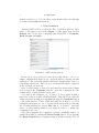
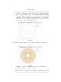
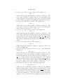
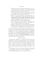
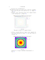
Starting ALF you’ll see a screen (see Fig. 1) which is split into three
parts: a left upper part labelled Input, a right upper part labelled
Output and a lower part containing buttons labelled ?, Compute,
Draw Graph, and Quit.
Figure 1. ALF’s main window
In the input part you’ll see several choices that allow to choose examples, implemented methods etc. and text fields for setting relevant
parameters. The text fields usually exhibit the default values of the corresponding parameters. These choices and text fields will be explained
in the following six sections.
Once you have made your choices and entered your favourite parameters you press the Compute button to start the computations. The
results will be depicted in the output part.
Note that some examples, e.g. solving a Poisson equation with a
sine-series solution, require additional input. This will be provided via
additional windows that show up after pressing the Compute Button
of the main window. These additional windows all have a top label
explaining their purpose, one or several labelled text fields for entering
the relevant parameters, and an OK button. You have to press the
latter one after having finished your input in order to continue the
computation process.
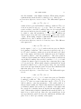
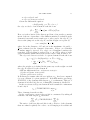
Once the computation is completed you may eventually want to visualise the results by clicking the Draw Graph button. Upon pressing
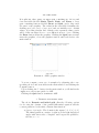
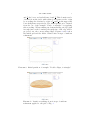
the Draw Graph button a graphics window will show up (see Fig. 2).
ALF USER GUIDE
3
It is split into three parts: an upper part containing two choices and
four text fields labelled Xmin, Xmax, Ymin, and Ymax, a lower
part containing buttons labelled Draw and Quit, and a large middle part for the graphics. The values in the text fields determine the
drawing area [xmin , xmax ] × [ymin , ymax ] and are initially set to default
values. Note that abscissa and ordinate scale separately, thus a circle
will look like an ellipse if xmax − xmin differs from ymax − ymin . Clicking
the Draw button starts the graphics. Clicking the Quit button terminates the graphics, closes the graphics window and leads back to the
main window.
Figure 2. ALF’s graphics window
You can compute a new set of examples by adjusting the corresponding choices and text fields in the main window and clicking the
Compute button.
Upon clicking the ? button in the main window you’ll find in the
output area a short user guide for ALF.
Clicking the Quit button terminates ALF.
3. Domain and initial grid
The choice Domain and initial grid offers the following options
for choosing the domain of the partial differential equation and the
coarsest partition for the finite element discretization:
• Square, 8 triangles: The domain is the square [−1, 1] × [−1, 1].
The initial partition consists of eight isosceles right-angled triangles with short sides of length 1 and longest side parallel to
the line y = −x.
4
¨
R. VERFURTH
• Square, 4 triangles: The domain is the square [−1, 1] × [−1, 1].
The initial partition is obtained by drawing the two diagonals
of the square.
• Square, 4 squares: The domain is the square [−1, 1] × [−1, 1].
The initial partition consists of four squares with sides of length
1.
• L-shaped, 6 triangles: The domain and initial partition are obtained by removing the square [0, 1] × [−1, 0] in the example
”Square, 8 triangles”.
• L-shaped, 3 squares: The domain and initial partition are obtained by removing the square [0, 1] × [−1, 0] in the example
”Square, 4 squares”.
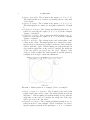
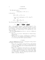
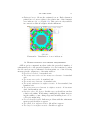
• Circle, 8 triangles: The domain is the circle with radius 1 and
centre at the origin. The initial partition is obtained by replacing the circle by an inscribed regular octahedron and joining its
vertices with the origin. When refining an element having an
edge with its endpoints on the circle’s boundary, the midpoint
of the edge will be projected onto the circle. Figures 3 and
4 show for this example the initial partition and the partition
resulting from 4 steps of uniform refinement.
Figure 3. Initial partition of example ”Circle, 8 triangles”
• Circle, 4 squares, 8 triangles: The domain is the circle with
radius 1 and centre at the origin. The initial partition is shown
in Figure 5. When refining an element having an edge with its
endpoints on the circle’s boundary, the midpoint of the edge
will be projected onto the circle.
• Segment, 6 triangles: The domain and initial partition are obtained from those of the example ”Circle, 8 triangles” by removing the quarter-segment in the quadrant x > 0, y < 0 and the
ALF USER GUIDE
5
Figure 4. Partition resulting from 4 steps of uniform
refinement applied to the grid of Fig. 3
Figure 5. Initial partition of the example ”Circle, 4
squares, 8 triangles”
corresponding elements. When refining an element having an
edge with its endpoints on the circle’s boundary, the midpoint
of the edge will be projected onto the circle.
• Segment, 3 squares, 6 triangles: The domain and initial partition are obtained from those of the example ”Circle, 4 squares,
8 triangles” by removing the quarter-segment in the quadrant
x > 0, y < 0 and the corresponding elements. When refining
an element having an edge with its endpoints on the circle’s
boundary, the midpoint of the edge will be projected onto the
circle.
6
¨
R. VERFURTH
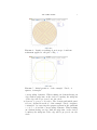
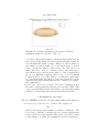
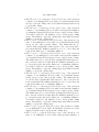
• Annulus, 12 triangles: The domain is the annulus, which is
formed by concentric circles with radii 0.25 and 1 and centre
at the origin. Figures 6 and 7 show for this example the initial
partition and the mesh that is obtained after 4 steps of uniform
refinement. When refining an element having an edge with its
endpoints on the boundary, the midpoint of the edge will be
projected onto the corresponding circle.
Figure 6. Initial partition of example ”Annulus, 12 triangles”
Figure 7. Partition resulting from 4 steps of uniform
refinement applied to the grid of Fig. 6
• Double ellipse, 8 triangles: The domain’s boundary consists of
two ellipses centred at the origin. The top one has half axes 1
ALF USER GUIDE
7
and 12 ; the lower one has half axes 1 and 14 . This domain can be
obtained from the circle with radius 1 and centre at the origin
by re-scaling the abscissa by a factor 12 and 14 in the upper and
lower half-planes respectively. The initial partition is obtained
from the one of the example ”Circle, 8 triangles” by applying
this re-scaling. When refining an element having an edge with
its endpoints on the boundary, the midpoint of the edge will be
projected onto the corresponding ellipse. Figures 8 and 9 show
the initial grid and the mesh obtained after 4 steps of uniform
refinement.
Figure 8. Initial partition of example ”Double ellipse, 8 triangles”
Figure 9. Partition resulting from 4 steps of uniform
refinement applied to the grid of Fig. 8
8
¨
R. VERFURTH
• Double ellipse, 4 squares, 8 triangles: The domain’s boundary
consists of two ellipses centred at the origin. The top one has
half axes 1 and 21 ; the lower one has half axes 1 and 14 . This
domain can be obtained from the circle with radius 1 and centre
at the origin by re-scaling the abscissa by a factor 12 and 14 in
the upper and lower half-planes respectively. The initial partition is obtained from the one of the example ”Circle, 4 squares,
8 triangles” by applying this re-scaling. When refining an element having an edge with its endpoints on the boundary, the
midpoint of the edge will be projected onto the corresponding
ellipse. Figures 10 and 11 show the initial grid and the mesh
obtained after 4 steps of uniform refinement.
Figure 10. Initial partition of example ”Double ellipse,
4 squares, 8 triangles”
• User defined initial grid : You are first asked to enter the number of nodes. Then you have to enter for each node its x- and
y-co-ordinates and a label that specifies whether the point lies
in the interior of the domain (label 0), or on a Dirichlet boundary (label > 0), or on a Neumann boundary (label < 0). Then
you are asked for the number of elements. Finally you have
to enter for each element four integers giving the global numbers of the element’s nodes. When the element is a triangle
the fourth number must be −1. The local enumeration of the
element vertices must be such that the element interior lies on
the left-hand side when passing through the element boundary
according to this enumeration.
• User defined boundary, automatic tessellation: The domain is
split into sub-domains that are each specified by an ordered list
ALF USER GUIDE
9
Figure 11. Partition resulting from 4 steps of uniform
refinement applied to the grid of Fig. 10
of vertices. Each sub-domain is automatically partitioned using a chop-off algorithm. The sub-domains and their partitions
are automatically glued together. First you will be asked for
the number of sub-domains. For each sub-domain, you then
have to specify the number of its vertices. For each vertex you
must enter its x- and y-co-ordinates and a label that specifies whether the point lies in the interior of the domain (label
0), or on a Dirichlet boundary (label > 0), or on a Neumann
boundary (label < 0). The vertices of each sub-domain must
be ordered such that the interior of the sub-domain lies on the
left-hand side when passing through its boundary according to
this enumeration.
• Initial grid of previous example: The next computation uses
the same coarsest partition as in the previous run of ALF. This
option is particularly useful when using a user-specified initial
partition or when using the automatic-tessellation-facility.
4. Differential equation
The choice PDE provides the following sample differential equations:
• Poisson equ. with sin-series solution: The equation is
−∆u = f
with non-homogeneous Dirichlet boundary conditions. The
force term f and the boundary data are chosen such that the
exact solution is a user-specified sine-series. You will be asked
for the number of terms, the amplitudes, and the frequencies.
10
¨
R. VERFURTH
• Poisson equ. with cos-series solution: The equation is
−∆u = f
with non-homogeneous Dirichlet boundary conditions. The
force term f and the boundary data are chosen such that the
exact solution is a user-specified cosine-series. You will be asked
for the number of terms, the amplitudes, and the frequencies.
• Poisson equ. with bubble solution: The equation is
−∆u = f
with non-homogeneous Dirichlet boundary conditions. The
force term f and the boundary data are chosen such that the
exact solution is given by (1 − x2 )(1 − y 2 ).
• Poisson equ. with singular solution: The equation is
−∆u = f
with non-homogeneous Dirichlet boundary conditions. The
force term f and the boundary data are chosen such that the
exact solution is given by the singular solution for a 34 -segment
2
that takes in polar co-ordinates the form r 3 sin( 23 ϕ). When using adaptive refinement the mesh should be refined close to the
origin.
• Poisson equ. with unit load : The equation is
−∆u = 1
with homogeneous Dirichlet boundary conditions. The exact
solution is unknown.
• Reaction-diffusion equation, interior layer : The differential
equation is
−∆u + bu = f
with non-homogeneous Dirichlet boundary conditions. The
force term f , the reaction term b, and the boundary data are
chosen such that the exact solution is given by tanh(κ(x2 + y 2 −
1
)). You will be asked to enter the parameter κ. The solution
4
exhibits an interior layer along the circle with radius 12 and centre at the origin. When using adaptive refinement the mesh
should be refined close to the boundary of this circle.
• Discontinuous diffusion: The differential equation is
−div(Dgradu) = 1
with homogeneous Dirichlet boundary conditions. The diffusion
matrix D is piecewise constant: in the region 4x2 + 16y 2 < 1 its
diagonal and off-diagonal elements are κ and κ(κ−1)
respectively;
κ+1
outside this region it is the identity matrix. You will be asked
to enter the parameter κ. The exact solution of this problem is
unknown, but it is known that it exhibits an interior layer at
ALF USER GUIDE
11
the discontinuity of the diffusion matrix. When using adaptive
refinement the mesh should be refined close to this region.
• Convection-diffusion, interior layer : The differential equation
is
−ε∆u + a · ∇u + bu = f
with non-homogeneous Dirichlet boundary conditions. The convection is given by a(x, y) = (−y, x)T . The force term f , the
reaction term b, and the boundary data are chosen such that
1
the exact solution is given by tanh(ε− 2 (x2 + y 2 − 14 )). You will
be asked to enter the parameter ε. The solution exhibits an
interior layer along the circle with radius 12 and centre at the
origin. When using adaptive refinement the mesh should be
refined close to the boundary of this circle.
• Convection-diffusion, interior & boundary layer : The differential equation is
−ε∆u + a · ∇u + bu = 0
in the square [−1, 1] × [−1, 1] with non-homogeneous Dirichlet boundary conditions. The convection is given by a(x, y) =
(2, 1)T ; the boundary condition is 0 at the left and top boundary of the square and 100 at the right and bottom boundary.
You will be asked to enter the parameter ε. The exact solution
of this problem is unknown. But it is known that it exhibits an
exponential boundary layer at the boundary x = 1, y > 0 and
a parabolic interior layer along the line connecting the points
(−1, 1) and (1, 0). When using adaptive refinement the mesh
should be refined close to these regions. Since the exponential
layer is far stronger than the parabolic layer the refinement will
first take place close to the region x = 1, y > 0.
• Convection-diffusion, 3 boundary layers: The differential equation is
−ε∆u + a · ∇u + bu = f
in the square [−1, 1] × [−1, 1] with homogeneous Dirichlet
boundary conditions. The convection is given by a(x, y) =
(0, 1−x2 )T ; the force term f takes the form (1−x2 )(1−y 2 ). You
will be asked to enter the parameter ε. The exact solution of
this problem is unknown. But it is known that it exhibits an exponential boundary layer at the top boundary of the square and
two parabolic boundary layers along the left and right boundaries. When using adaptive refinement the mesh should be refined close to these regions. Since the exponential layer is far
stronger than the parabolic layer the refinement will first take
place close to the top boundary of the square.
¨
R. VERFURTH
12
5. Discretization
The differential equation
−div(Dgradu) + a · ∇u + bu = f
is discretized by
Z
∇u · D∇v + a · ∇uv + buv
Ω
Z
X
+
δK (−div(Dgradu) + a · ∇u + bu)a · ∇v
K∈Th
Z
fv +
=
Ω
K
X
K∈Th
Z
f a · ∇v.
δK
K
The SUPG-stabilisation parameters are given by
hK
2ε
kak2 hK
δK =
)−
coth(
,
2kak2
2ε
kak2 hK
where ε is the smallest eigenvalue of the diffusion matrix D. Nonhomogeneous Dirichlet boundary conditions are taken into account by
homogenisation. Non-homogeneous Neumann boundary data g give
rise to an additional boundary integral on the right-hand side of the
discrete problem.
The choice Discretization provides two options for building the
discrete problem:
• With numerical quadrature: All integrals are evaluated using a
midpoint rule.
• Without numerical quadrature. All integrals are evaluated exactly subject to the assumption that all functions (u, v, D, a,
b, f etc.) are piecewise linear respectively bilinear.
6. Solver
The choice Solver allows you to choose among the following solution
algorithms for the discrete problems:
• MG V-cycle, 1/2 symmetric Gauss-Seidel step: One iteration
consists of one multigrid V-cycle with one forward Gauss-Seidel
sweep for pre-smoothing and one backward Gauss-Seidel sweep
for post-smoothing.
• MG V-cycle, n symmetric Gauss-Seidel steps: One iteration
consists of one multigrid V-cycle with a user-specified number
of symmetric Gauss-Seidel sweeps for pre- and post-smoothing.
You will be asked for the number of pre- and post-smoothing
steps. The number of pre-smoothing steps may differ from the
number of post-smoothing steps.
ALF USER GUIDE
13
• MG W-cycle, 1/2 symmetric Gauss-Seidel step: One iteration
consists of one multigrid W-cycle with one forward Gauss-Seidel
sweep for pre-smoothing and one backward Gauss-Seidel sweep
for post-smoothing.
• MG W-cycle, n symmetric Gauss-Seidel steps: One iteration
consists of one multigrid W-cycle with a user-specified number
of symmetric Gauss-Seidel sweeps for pre- and post-smoothing.
You will be asked for the number of pre- and post-smoothing
steps. The number of pre-smoothing steps may differ from the
number of post-smoothing steps.
• MG V-cycle, 1 downwind Gauss-Seidel step: One iteration consists of one multigrid V-cycle with one downwind Gauss-Seidel
sweep for pre- and post-smoothing. The unknowns are reordered lexicographically with respect to the convection direction such that the stiffness matrix is close to lower diagonal
form in the limit case of vanishing diffusion.
• MG V-cycle, n downwind Gauss-Seidel steps: One iteration
consists of one multigrid V-cycle with a user-specified number
of downwind Gauss-Seidel sweeps for pre- and post-smoothing.
The unknowns are re-ordered lexicographically with respect to
the convection direction such that the stiffness matrix is close
to lower diagonal form in the limit case of vanishing diffusion.
You will be asked for the number of pre- and post-smoothing
steps. The number of pre-smoothing steps may differ from the
number of post-smoothing steps.
• MG W-cycle, 1 downwind Gauss-Seidel step: One iteration
consists of one multigrid W-cycle with one downwind GaussSeidel sweep for pre- and post-smoothing. The unknowns are
re-ordered lexicographically with respect to the convection direction such that the stiffness matrix is close to lower diagonal
form in the limit case of vanishing diffusion.
• MG W-cycle, n downwind Gauss-Seidel steps: One iteration
consists of one multigrid W-cycle with a user-specified number
of downwind Gauss-Seidel sweeps for pre- and post-smoothing.
The unknowns are re-ordered lexicographically with respect to
the convection direction such that the stiffness matrix is close
to lower diagonal form in the limit case of vanishing diffusion.
You will be asked for the number of pre- and post-smoothing
steps. The number of pre-smoothing steps may differ from the
number of post-smoothing steps.
• MG V-cycle, 1 squared Richardson step: One iteration consists
of one multigrid V-cycle with one Richardson iteration for the
squared system as pre- and post-smoothing step.
• MG V-cycle, n squared Richardson steps: One iteration consists of one multigrid V-cycle with a user-specified number of
14
¨
R. VERFURTH
Richardson iterations for the squared system as pre- and postsmoothing step. You will be asked for the number of pre- and
post-smoothing steps. The number of pre-smoothing steps may
differ from the number of post-smoothing steps.
• MG W-cycle, 1 squared Richardson step: One iteration consists
of one multigrid W-cycle with one Richardson iteration for the
squared system as pre- and post-smoothing step.
• MG W-cycle, n squared Richardson steps: One iteration consists of one multigrid W-cycle with a user-specified number of
Richardson iterations for the squared system as pre- and postsmoothing step. You will be asked for the number of pre- and
post-smoothing steps. The number of pre-smoothing steps may
differ from the number of post-smoothing steps.
• CG: This is a classical conjugate-gradient algorithm.
• CG with SSOR preconditioning: This is a classical preconditioned conjugate-gradient algorithm with one symmetric successive over-relaxation sweep for preconditioning.
• BiCG-Stab: This is a stabilised bi-conjugate-gradient algorithm.
• BiCG-Stab with SSOR preconditioning: This is a stabilised and
preconditioned bi-conjugate-gradient algorithm with one symmetric successive over-relaxation sweep for preconditioning.
All solution algorithms terminate when either M AXIT iterations have
been performed or when the initial residual, measured in the Euclidean
norm, has been reduced by at least a factor T OL. The parameter
M AXIT is set to 10 for the multigrid algorithms with Gauss-Seidel
smoothing, to 50 for the multigrid algorithms with squared Richardson
smoothing and to 100 for the CG and BiCG algorithms. The parameter
T OL is set to 0.01. The choice Solution parameters gives you the
opportunity to modify these parameters by choosing the option user
settings the standard choice being default.
7. Mesh refinement
ALF starts its computations on a partition, which is labelled Level
1 and which is obtained by a uniform refinement of the coarsest mesh
labelled Level 0 of the actual example. Having computed the discrete
solution on a mesh of Level k the partition of the next level is obtained
either by a uniform refinement or by an adaptive refinement based on
various a posteriori error indicators and refinement strategies. This
process is repeated until the prescribed number of refinement levels is
reached or until the allocated storage is exhausted (cf. Sections 8 and
10).
When using a uniform refinement every element is refined regularly,
i.e. the midpoints of edges are connected for triangles and the midpoints of opposite edges are connected for quadrilaterals.
ALF has implemented two types of residual error indicators:
ALF USER GUIDE
15
• edge residuals and
• edge and element residuals.
Given the differential equation
−div(Dgradu) + a · ∇u + bu = f
the edge residuals of an element K take the form
X
1
2
=
ηK
− 4 αE k[nE · D∇uh ]E k2L2 (E) .
E⊂∂K
Here, uh is the solution of the discrete problem, denotes the geometric
mean of the two eigenvalues of the diffusion matrix D evaluated at the
element’s barycentre, nE is a unit vector orthogonal to the edge E, [·]E
denotes the jump across the edge E, and the weight αE is given by
1
1
αE = min{hE − 2 , β − 2 },
where hE is the diameter of E and βE is the maximum of 0 and b −
1
diva evaluated at the element’s barycentre. Edges on a Dirichlet
2
boundary must be ignored. For edges on a Neumann boundary the
term [nE · D∇uh ]E must be replaced by g − n · D∇uh where g is the
given Neumann datum and n denotes the exterior unit normal to Ω.
The edge and element residuals of a given element K take the form
2
2
ηK
= αK
kf + div(Dgradu) − a · ∇u − buk2L2 (K)
X
1
− 4 αE k[nE · D∇uh ]E k2L2 (E) ,
+
E⊂∂K
where the weight αK is defined in the same way as the weight αE with
the edge E replaced by the element K.
ALF has implemented two refinement strategies:
(1) the maximum strategy and
(2) the equilibration strategy.
Both strategies assume that an error indicator ηK has been computed
for every element of a given partition T . Both first mark a percentage
EXCESS of the elements with largest ηK for refinement. This set of
elements is labelled M0 the set of unmarked elements is labelled U
In the maximum strategy an element K in U is marked for refinement
if and only if
ηK ≥ T HRESHOLD · max
ηK 0 .
0
K ∈U
These elements form the set M1 .
In the equilibration strategy the set M1 is constructed by taking all
elements of U with largest ηK such that
X
X
2
2
ηK
≥ T HRESHOLD ·
ηK
.
K∈M1
K∈U
The union of the sets M0 and M1 is the collection of the elements
that are refined regularly. In order to avoid hanging nodes additional
16
¨
R. VERFURTH
elements are refined green or blue as described in the literature (cf. e.g.
Chapter 4 of R. Verf¨
urth: A Review of A Posteriori Error Estimation
and Adaptive Mesh-Refinement Techniques. Wiley-Teubner 1996 or
Chapters III.3 and III.4 of the Lecture Notes Numerische Behandlung
von Differentialgleichungen II (Finite Elemente)).
The choice Mesh refinement allows you to choose among the implemented refinement and error estimation algorithms.
The choice Refinement parameters allows you to choose the parameters EXCESS and T HRESHOLD described above and the parameter F IRST ADAP T IV E that determines the first level on which
an adaptive refinement is performed. The default settings are
• EXCESS = 0.1,
• T HRESHOLD = 0.5,
• F IRST ADAP T IV E = 1.
When choosing the option user settings you will be asked to enter these
three parameters.
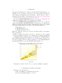
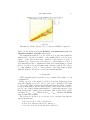
Figure 12 shows the mesh of Level 8 obtained for the example
”Convection-diffusion, interior & boundary layer” with the parameter
ε = 0.000001 and the default settings for EXCESS, T HRESHOLD,
and F IRST ADAP T IV E. Figure 13 shows the mesh of Level 7 for
the same example with the same parameters ε and T HRESHOLD
but with EXCESS = 0.2 and F IRST ADAP T IV E = 2.
Figure 12. Mesh of Level 8 for a convection-diffusion equation
8. Number of nodes and levels
LF has two key-parameters:
• M L: the number of refinement levels and
• M N : the maximal number of nodes.
ALF USER GUIDE
17
Figure 13. Mesh of Level 7 for a convection-diffusion equation
These are set in the text fields Number of refinement levels and
Maximal number of nodes respectively.
The refinement-solution loop (cf. Section 7) is performed until the
number M L of levels is reached, or the number M N of nodes is attained, or the allocated storage, which is a fixed factor of M N , is
exhausted (cf. Section 10). Choosing a too small number of M L or
M N naturally leads to computations with only a small number of grids
that do not allow for an adequate finite element solution. Choosing a
too large number of M L or – most critical – M N may cause troubles
with the memory allocation of your Java virtual machine.
9. Graphics
ALF’s graphics window enables you to visualise the results of your
computations.
In the top row of the window you’ll see four text fields that determine the clipping area [xmin , xmax ] × [ymin , ymax ]. Usually you’ll want
to choose the values in these text fields such that the whole computational domain will be shown. But selecting other values allows you to
get a zoom of sub-domains that might be of particular interest. Note
that abscissa and ordinate scale separately, thus a circle will look like
an ellipse if xmax − xmin differs from ymax − ymin . Clicking the Draw
button starts the graphics.
The left choice in the top row allows you to navigate through the
various mesh-levels:
• First level : Go to the coarsest level.
• Next level : Increase the level count by 1.
• Previous level : Decrease the level count by 1.
18
¨
R. VERFURTH
• Last level : Go to the finest level.
The right choice in the top row lets you choose the type of graphics:
• Grid : Shows the grid of the actual level (cf. e.g. Figures 12
and 13).
• Solution: isolines: Shows the isolines of the computed solution
on the actual grid (cf. e.g. Figure 14).
Figure 14. Isolines of a computed solution
• Solution: colourplot: Shows a colourplot of the computed solution on the actual grid (cf. Figure 15 for the same solution as
in Figure 14).
Figure 15. Colourplot of the finite element function of
Fig. 14
ALF USER GUIDE
19
• Estimated error : Shows the estimated errors. Each element is
painted in a colour according to the relative size of the element’s
error indicator (cf. e.g. Figure 16). This option is only available
in connection with an adaptive mesh refinement.
Figure 16. Visualisation of error indicators
10. Error handling and memory requirement
ALF stops its computations when either the prescribed number of
refinement levels or the prescribed number of nodes is attained or when
the allocated storage is exhausted. It then prints one of the following
messages in the output area of its main window:
• Final level reached : A standard exit.
• Too many new nodes and too many new elements: A standard
exit.
• Too many new nodes: A standard exit.
• Too many new elements: A standard exit.
• Too many unknowns in stiffness matrix : A less standard, but
harmless exit.
• Too many non-zero elements in stiffness matrix : A less standard, but harmless exit.
• Iterative solver did diverge: In this case you should try another
solution algorithm. When using a multigrid algorithm, increasing the number of smoothing steps and switching from a V- to
a W-cycle might help.
• No red elements found : Indicates problems with the refinement
strategy and should not appear.
• Too small lv in stiffness matrix : Should not appear.
• Too large lv in stiffness matrix : Should not appear.
20
¨
R. VERFURTH
Sometimes user-input data may be erroneous. ALF then prints an
error message and stops the computation. In this case you may try
to compute the same example with a new input or a completely new
example. The following error messages may be encountered:
• Inconsistent neighbour relation: Indicates an erroneous userinput when using the options ”user defined initial grid” or ”user
defined boundary, automatic tessellation”.
• Inconsistent node data: Indicates an erroneous user-input when
using the options ”user defined initial grid” or ”user defined
boundary, automatic tessellation”.
• Inconsistent element data: Indicates an erroneous user-input
when using the options ”user defined initial grid” or ”user defined boundary, automatic tessellation”.
• No neighbour found for element ... with index at least ...: Indicates an erroneous user-input when using the options ”user
defined initial grid” or ”user defined boundary, automatic tessellation”.
• Too many nodes in first grid : Should not appear.
• Too many elements in first grid : Should not appear.
• Non-existing initial grid : Should not appear.
• No elements in first grid : Should not appear.
When using a too large number of refinement levels or – more critical
– a too large number of nodes, your Java virtual machine may run out
of memory. It then throws an out of memory exception. ALF tries to
catch this exception. In this case ALF prints the error message Error:
insufficient memory. You then have to re-launch the applet.
If the error message did occur with your first example, you probably
have chosen a too large a number of nodes. In this case you should
enter a smaller number in the text field Maximum number of nodes
and try again.
If the error message occurs after several successful computations,
Java’s garbage collector probably has not done its job. In this case
you may try again with your old settings of the text field Maximum
number of nodes.
ALF requires about 50M N doubles and 60M N integers where M N
is the number given in the text field Maximum number of nodes.
¨t Bochum, Fakulta
¨t fu
¨r Mathematik, D-44780 BoRuhr-Universita
chum, Germany
E-mail address: [email protected]