Download AFEM USER GUIDE Contents 1. Introduction 1 2. Installing Scilab 2

AFEM USER GUIDE
¨
R. VERFURTH
Contents
1. Introduction
2. Installing Scilab
3. Installing AFEM
4. Using AFEM
4.1. Data structures
4.2. Start
4.3. Help
5. Function afem
5.1. Overview
5.2. Dimensions
5.3. Predefined sample equations and discretizations
5.4. Coefficients and right-hand side of the differential equation
5.5. Initial mesh and domain
5.6. Error estimation and mesh refinement
5.7. Print and plot output
References
Index
1
2
2
3
3
4
4
4
4
5
6
10
11
12
13
14
15
1. Introduction
AFEM is a library of Scilab functions implementing an adaptive linear
finite element method for general linear elliptic equations of second
order in a bounded connected two dimensional domain with mixed
Dirichlet, Neumann or Robin boundary conditions
− div(A∇u) + a · ∇u + αu = f
u = uD
n · A∇u = g
ρu + n · A∇u = g
in Ω
on ΓD
on ΓN
on ΓR .
The discretization consists of standard linear triangular elements without any additional stabilization and uD replaced by its linear interpolate IT uD :
Date: January 5, 2012.
1
2
¨
R. VERFURTH
1,0
Find uT ∈ IT uD + SD
(T ) such that
Z
(∇uT · A∇vT + a · ∇uT vT + αuT vT )
Ω
Z
Z
Z
ρuT vT =
f vT +
+
ΓR
Ω
gvT
ΓN ∪ΓR
1,0
holds for all vT ∈ SD
(T ).
Notice that the domain Ω may have a curved boundary. In this case the
integrals in the discrete problem extend over piecewise linear approximations of Ω and its boundary. The assembly is based on quadrature
rules of order one and two. The discrete problem is solved using the
built-in sparse linear system solver of Scilab. The mesh refinement is
either uniform or adaptive with marked edge bisection based on either
a standard residual error indicator, or a residual error indicator based
on edge residuals exclusively, or the Zinkiewicz-Zhu error estimator in
its simplest form. We refer to [4, 5] for a more detailed description of
the mathematical background.
A detailed description of AFEM and its main function afem are given
in sections 4 and 5 below. In sections 2 and 3 we first explain how to
install Scilab and AFEM, respectively.
2. Installing Scilab
Scilab is a numerical programming environment comparable to
Matlab with a similar syntax. It was developed by INRIA, France and is
currently maintained by the Digiteo-foundation in collaboration with
INRIA. Contrary to Matlab, Scilab is completely free of charge. There
are versions for the operating systems Mac OsX, Unix and Windows. To
use AFEM you first have to get the appropriate version of Scilab from
http://www.scilab.org/
and install it on your computer following the instructions of that website. Useful introductions to Scilab are e.g. [1, 2]; [3] may be of particular interest for those familiar with Matlab.
3. Installing AFEM
To install AFEM click the link AFEM.zip on
http://www.rub.de/num1/softwareE.html
or
http://www.rub.de/num1/software.html.
This installs a zip-archive AFEM.zip on your computer. Unpack the ziparchive and put the created folder AFEM at any place on your computer
that suits you. Now you can start AFEM as described in section 4.3.
AFEM USER GUIDE
3
4. Using AFEM
4.1. Data structures. We refer to [1, 2, 3] for a detailed introduction
to Scilab. Here, we briefly present those data structures of Scilab
that are used for input arguments of AFEM’s main function afem.
Boolean: Boolean arguments are transferred to afem by either directly
entering %t for the value true or %f for the value false or by creating an own boolean variable myboolean by typing myboolean = %t
or myboolean = %f in the Scilab console and then calling afem with
myboolean as argument.
String: Strings are enclosed by quotation marks. They are transferred
to afem by either directly entering "name" for the string value name
or by creating an own string variable mystring by typing mystring =
"name" in the Scilab console and then calling afem with mystring as
argument.
Number: Numbers may be integers like 2 and −3 or fixed point reals like 3.14 and −2.87 or floating point reals like 0.578D4, −0.689D5,
0.203D−7, and −0.1763D−5. They are transferred to afem by either
directly entering the numerical value or by creating an own variable
mynumber by typing mynumber = 2 or similar in the Scilab console
and then calling afem with mynumber as argument.
Vector / Matrix: A vector is either an m×1 matrix for a column vector
or a 1 × n matrix for a row vector. Matrices are created by typing the
appropriate sequence of numbers in lexicographic order from top left to
bottom right in brackets with columns separated by blanks or commas
and rows separated by semicolons. Thus the matrices


1 2
1 2 3
and 3 4
4 5 6
5 6
are represented by
[1 2 3; 4 5 6] and [1, 2; 3, 4; 5, 6].
A0 is the transpose of the matrix A; A ∗ B is the product of the matrices A and B. ones(m, n) and zeros(m, n) create m × n matrices
with all elements equal to 1 and 0, respectively; eye(n, n) creates the
n × n identity matrix. Matrices are transferred to afem by either directly entering the matrix or by creating an own matrix-valued variable
mymatrix and then calling afem with mymatrix as argument.
List: A list is an ordered collection of objects of different types. It may
be passed directly to afem by entering list(obj1,...,objn) for the
corresponding argument. Here, obj1, . . ., objn is a sequence of arbitrary length of objects of arbitrary types such as numbers, matrices,
functions, lists etc. Alternatively you my first create an own variable
of type list by entering
mylist = list(obj1,...,objn)
4
¨
R. VERFURTH
in the Scilab console and then call afem with mylist as argument.
Function: Functions, user-defined or built-in ones, are transferred to
afem by entering their name for the corresponding argument. For a
user-defined function, however, you first have to create a corresponding
variable. To clarify this, suppose that you want to use the function
1 + 2x21 + 5x22 as right-hand side f of the differential equation. Then
you first enter
function y = myforce(x)
y = 1 + 2∗x(1)∗x(1) + 5∗x(2)∗x(2)
endfunction
in the Scilab console and then use myforce as the corresponding argument of afem.
4.2. Start. Before using AFEM you must make it known to Scilab by
first entering
mylib = lib(path)
to the console. Here, mylib may be any other name different from
the name of any AFEM function, any built-in function and any of your
user-defined functions. path is a string giving the full path to the
AFEM library. Suppose for example that you are using Mac OsX, that
Gargantua is your user name and that you have put the AFEM folder
into the subfolder Pantagruel of your documents folder. Then the
above command must read (without the full stop at the end!)
mylib = lib("/users/Gargantua/documents/Pantagruel/AFEM").
If everything is correctly installed, Scilab returns the names of all
functions in the AFEM library. This includes auxiliary functions which
are not user-relevant and which will not be described below.
4.3. Help. AFEM comes with a help function afem help which has an
empty argument list and which yields a brief information about the
arguments of the main function afem and their use.
5. Function afem
5.1. Overview. AFEM’s main function is afem. It has several arguments which allow to adjust the parameters of the differential equation, of its discretization and of the adaptive process and which will be
described in more detail in the following subsections.
Each argument has a default value so that afem may be called with an
empty argument list. When entering
afem()
in the Scilab console, the Poisson equation
−∆u = 1 in Ω
u = 0 on Γ
AFEM USER GUIDE
5
is solved on the square Ω = (−1, 1)2 with uniform mesh refinement
starting from a criss-cross grid with eight triangles (see left part of
figure 5.1).
Since this example is not very exciting you probably want to adjust
some arguments. This is achieved by entering
afem(init param(key1,value1,..,keyn,valuen))
in the Scilab console. Here, key1, . . ., keyn is any number of any of
the keywords described in the following subsections in any order and
value1, . . ., valuen are the corresponding values. The latter can be
booleans, strings, numbers, matrices, lists or functions depending on
the corresponding keyword. Notice that keywords are strings and must
be enclosed by quotation marks. To clarify this consider two simple
examples.
Suppose that you want to replace the constant right-hand side 1 in the
above example by the function 1 + 2x21 + 5x22 and that you have defined
the corresponding function myforce as described at the end of section
4.1. Then you must enter
afem(init param("force",myforce))
in the console.
Suppose that you now want to try an adaptive refinement based on the
maximum strategy and the error estimator based on edge residuals.
Then you must enter
afem(init param("force",myforce,"reftype",1))
in the console. Note that entering
afem(init param("reftype",1,"force",myforce))
will produce the same result while entering
afem(init param("force",1,"reftype",myforce))
will result in an error message since the types of the values do not fit
with the keywords (1 is not a function, myforce is not a number!).
5.2. Dimensions. The behaviour of afem and its storage requirement
is controlled by two keywords:
maxnodes: determines the maximal number of nodes i.e. vertices
of elements. Its default value is 10000. The maximal number
of elements in a single mesh is automatically set to 2 maxnodes,
the maximal cumulative number of elements over all meshes is
automatically set to 6 maxnodes.
maxlevels: determines the maximal number of refinement levels.
Its default value is 21.
Instead of prescribing the keywords maxnodes and maxlevels with
corresponding values, you may also control the behaviour of afem and
its storage requirement by entering the keyword dimensions followed
6
¨
R. VERFURTH
by an integer vector of length four as value. The four components of
this vector have the following meaning:
(1) maximal number of levels, default is 21,
(2) maximal number of nodes, default is 10000,
(3) maximal number of elements on a single level, default is 20000,
(4) maximal cumulative number of elements on all levels, default is
60000.
Thus the pair
"dimensions",[12,1000,2000,6000]
in your parameter list has the same effect as the two pairs
"maxlevels",12 and "maxnodes",1000
in the list. Notice that the pair
"dimensions",[12,1000,3000,8000]
would correspond to the same number of levels and the same maximal number of nodes but would allow for the bigger maximal number
3000 of elements on a single mesh and the bigger maximal cumulative
number 8000 of elements on all meshes.
5.3. Predefined sample equations and discretizations. The keyword sample pde allows you to use predefined sample equations and
discretizations. The corresponding value must be list. The length of
this list depends on the example as explained below. Its first argument
always is a string which specifies the example. If the list’s length is 1
you may only enter this string as value. Thus the pairs
"sample pde",list("l1sq") and "sample pde","l1sq"
in your parameter list both have the same effect. Notice that the use
of the keyword sample pde together with a corresponding value overrides the settings of the keywords diffusion, convection, reaction,
force, traction, robin, bdrydispl and solution described in subsection 5.4. If the chosen example also specifies a domain and initial
mesh, the settings of the keywords sample mesh, init node, init elem
and domain described in subsection 5.5 are also overridden. sample pde
allows you to choose among the following examples:
l0u1sq: Laplace equation −∆u = 0 with Dirichlet boundary condition and exact solution 1 on the square (−1, 1)2 subdivided
into 8 isosceles right-angled triangles (see left part of figure 5.1).
lubsq: Laplace equation −∆u = f with Dirichlet boundary condition and exact solution (1 − x21 )(1 − x22 ) on the square (−1, 1)2
subdivided into 8 isosceles right-angled triangles (see left part
of figure 5.1).
l1: Laplace equation −∆u = 1 with homogeneous Dirichlet
boundary condition, the domain and initial mesh must be prescribed separately.
AFEM USER GUIDE
7
l1sq: Laplace equation −∆u = 1 with homogeneous Dirichlet
boundary condition on the square (−1, 1)2 subdivided into 8
isosceles right-angled triangles (see left part of figure 5.1).
l1c: Laplace equation −∆u = 1 with homogeneous Dirichlet
boundary condition on the unit circle x21 + x22 < 1 subdivided
into 8 triangles (see left part of figure 5.2).
l1a: Laplace equation −∆u = 1 with homogeneous Dirichlet
1
boundary condition on the annulus 16
< x21 + x22 < 1 subdivided into 16 triangles (see figure 5.3).
2
2 1 2
lg: Laplace equation −∆u = e−κ(x1 +x2 − 4 ) with κ given by second argument, the domain and initial mesh must be prescribed
separately.
lilsq: Laplace equation −∆u = f with Dirichlet
boundary condition and exact solution tanh κ x21 + x22 − 14 on the square
(−1, 1)2 subdivided into 8 isosceles right-angled triangles (see
left part of figure 5.1) and κ given by second argument.
lilc: Laplace equation −∆u = f with Dirichletboundary condition and exact solution tanh κ x21 + x22 − 14 on the circle
x21 + x22 < 1 subdivided into 8 triangles (see left part of figure
5.2) and κ given by second argument.
lila: Laplace equation −∆u = f with Dirichletboundary condition and exact solution tanh κ x21 + x22 − 41 on the annulus
1
< x21 + x22 < 1 subdivided into 16 triangles (see figure 5.3)
16
and κ given by second argument.
lilrsq: Laplace equation −∆u = f with Dirichlet boundary condition and exact solution 1+κ2 (x21+x2 − 1 )2 on the square (−1, 1)2
1
2 4
subdivided into 8 isosceles right-angled triangles (see left part
of figure 5.1) and κ given by second argument.
lilrc: Laplace equation −∆u = f with Dirichlet boundary condition and exact solution 1+κ2 (x21+x2 − 1 )2 on the circle x21 +x22 < 1
1
2 4
subdivided into 8 triangles (see left part of figure 5.2) and κ
given by second argument.
lilra: Laplace equation −∆u = f with Dirichlet boundary con1
dition and exact solution 1+κ2 (x21+x2 − 1 )2 on the annulus 16
<
1
2
4
x21 + x22 < 1 subdivided into 16 triangles (see figure 5.3) and κ
given by second argument.
lssl: Laplace equation −∆u = 0 with Dirichlet boundary con2
dition and exact solution r 3 sin( 23 ϕ) on the L-shaped domain
(−1, 1)2 \(0, 1)×(−1, 0) subdivided into 6 isosceles right-angled
triangles (see right part of figure 5.1).
lsscs: Laplace equation −∆u = 0 with Dirichlet boundary condi2
tion and exact solution r 3 sin( 23 ϕ) on the circular sector
8
¨
R. VERFURTH
{(r cos ϕ, r sin ϕ) : 0 ≤ r < 1, 0 ≤ ϕ ≤ 32 π} subdivided into
6 triangles (see right part of figure 5.2).
dru1sq: Diffusion reaction equation −∆u + κu = 1 with Dirichlet
boundary condition and exact solution 1 on the square (−1, 1)2
subdivided into 8 isosceles right-angled triangles (see left part of
figure 5.1) and κ given by second argument, e.g. "sample pde",
list("dru1sq",100) sets κ = 100.
drbru1sq: Diffusion reaction equation
−∆u + κ(1 − x21 )(1 − x22 )u = κ(1 − x21 )(1 − x22 )
with Dirichlet boundary condition and exact solution 1 on the
square (−1, 1)2 subdivided into 8 isosceles right-angled triangles
(see left part of figure 5.1) and κ given by second argument, e.g.
"sample pde",list("drbru1sq",100) sets κ = 100.
drubsq: Diffusion reaction equation −∆u + κu = f with Dirichlet
boundary condition and exact solution (1 − x21 )(1 − x22 ) on the
square (−1, 1)2 subdivided into 8 isosceles right-angled triangles
(see left part of figure 5.1) and κ given by second argument, e.g.
"sample pde",list("drubsq",100) sets κ = 100.
drbrubsq: Diffusion reaction equation
−∆u + κ(1 − x21 )(1 − x22 )u = f
with Dirichlet boundary condition and exact solution (1 − x21 )
(1 − x22 ) on the square (−1, 1)2 subdivided into 8 isosceles rightangled triangles (see left part of figure 5.1) and κ given by
second argument, e.g. "sample pde",list("drbrubsq",100)
sets κ = 100.
drilsq: Diffusion reaction equation −∆u + κu = f with Dirichlet
boundary condition and exact solution tanh κ x21 + x22 − 14
on the square (−1, 1)2 subdivided into 8 isosceles right-angled
triangles (see left part of figure 5.1) and κ given by second
argument, e.g. "sample pde",list("drilsq",100) sets κ =
100.
drilc: Diffusion reaction equation −∆u + κu = f with Dirichlet
boundary condition and exact solution tanh κ x21 + x22 − 14
on the circle x21 + x22 < 1 subdivided into 8 triangles (see
left part of figure 5.2) and κ given by second argument, e.g.
"sample pde",list("drilc",100) sets κ = 100.
drila: Diffusion reaction equation −∆u + κu = f with Dirichlet
boundary condition and exact solution tanh κ x21 + x22 − 41
1
on the annulus 16
< x21 + x22 < 1 subdivided into 16 triangles (see figure 5.3) and κ given by second argument, e.g.
"sample pde",list("drila",100) sets κ = 100.
AFEM USER GUIDE
9
drilch: Diffusion reaction equation −∆u + κu = f with Dirichlet
boundary condition and exact solution
61
196
− x21 − x22 )) + tanh(κ 257
)
tanh(κ( 257
61
196
tanh(κ 257 ) + tanh(κ 257 )
on the circle x21 + x22 < 1 subdivided into 8 triangles (see
left part of figure 5.2) with κ given by second argument, e.g.
"sample pde",list("drilch",100) sets κ = 100.
dciblsq: Anisotropic diffusion convection equation
∂ 2u ∂ 2u
∂u
∂u
−
+
2
+
=0
∂x21 ∂x22
∂x1 ∂x2
with Dirichlet boundary condition


if x2 = 1
1
uD (x) = −1 if x2 = −1

0
else
−ε
on the square (−1, 1)2 subdivided into 8 isosceles right-angled
triangles (see left part of figure 5.1) and ε given by second argument, e.g. "sample pde",list("dciblsq",0.001) sets ε =
0.001.
aidsq: Anisotropic diffusion equation
∂ 2u ∂ 2u
−
=0
∂x21 ∂x22
with Dirichlet boundary condition


if x2 = 1
1
uD (x) = −1 if x2 = −1

0
else
−ε
on the square (−1, 1)2 subdivided into 8 isosceles right-angled
triangles (see left part of figure 5.1) and ε given by second
argument, e.g. "sample pde",list("aidsq",0.001) sets ε =
0.001.
cbdsq: Checker-board diffusion equation −d∆u = 0 with
(
ε if x1 x2 < 0
d=
1 else
and Dirichlet boundary


0
uD (x) = 1

−1
condition
if x1 x2 < 0
if x1 x2 ≥ 0 and x1 ≥ 0
if x1 x2 ≥ 0 and x1 ≤ 0
on the square (−1, 1)2 subdivided into 8 isosceles right-angled
triangles (see left part of figure 5.1) and ε given by second
¨
R. VERFURTH
10
argument, e.g. "sample pde",list("cbdsq",0.001) sets ε =
0.001.
mesh of level 1 with 8 elements and 9 nodes
mesh of level 1 with 6 elements and 8 nodes
1.0
1.0
0.8
0.8
0.6
0.6
0.4
0.4
0.2
0.2
0.0
0.0
- 0.2
- 0.2
- 0.4
- 0.4
- 0.6
- 0.6
- 0.8
- 1.0
- 1.0
- 0.8
- 0.8
- 0.6
- 0.4
- 0.2
0.0
0.2
0.4
0.6
0.8
1.0
- 1.0
- 1.0
- 0.8
- 0.6
- 0.4
- 0.2
0.0
0.2
0.4
0.6
0.8
1.0
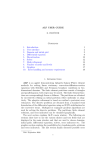
Figure 5.1. Initial mesh for a square (left) and an Lshaped domain (right)
mesh of level 1 with 8 elements and 9 nodes
mesh of level 1 with 6 elements and 8 nodes
1.0
1.0
0.8
0.8
0.6
0.6
0.4
0.4
0.2
0.2
0.0
0.0
- 0.2
- 0.2
- 0.4
- 0.4
- 0.6
- 0.6
- 0.8
- 0.8
- 1.0
- 1.0
- 0.8
- 0.6
- 0.4
- 0.2
0.0
0.2
0.4
0.6
0.8
1.0
- 1.0
- 1.0
- 0.8
- 0.6
- 0.4
- 0.2
0.0
0.2
0.4
0.6
0.8
1.0
Figure 5.2. Initial mesh for a circle (left) and a circular
sector (right)
5.4. Coefficients and right-hand side of the differential equation. The following keywords with functions as corresponding values
allow to prescribe the coefficients and right-hand side of the differential
equation:
diffusion: diffusion A, default is A = ( 10 01 ),
convection: convection a, default is a = 0,
reaction: reaction α, default is α = 0,
force: right-hand side f , default is f = 1,
traction: right-hand side g, default is g = 0,
robin: function ρ in Robin condition, default is ρ = 0,
bdrydispl: boundary displacement uD , default is uD = 0.
AFEM USER GUIDE
11
mesh of level 1 with 16 elements and 16 nodes
1.0
0.8
0.6
0.4
0.2
0.0
- 0.2
- 0.4
- 0.6
- 0.8
- 1.0
- 1.0
- 0.8
- 0.6
- 0.4
- 0.2
0.0
0.2
0.4
0.6
0.8
1.0
Figure 5.3. Initial mesh for an annulus with radii
1
4
and 1
Notice that adopting all default values yields the Laplace equation
−∆u = 1 with homogeneous Dirichlet boundary condition. Also recall
that prescribing the keyword sample pde described in subsection 5.3
overrides the settings of the above keywords.
The keyword solution allows to prescribe an eventually known exact solution of the differential equation. Its value must be a vector of
length two with its first argument either %t for a known exact solution or %f for an unknown exact solution and its second argument a
built-in or user-defined function giving the exact solution. The default
setting is [%f,unit function] where unit function corresponds to
the function u = 1 which is among AFEM’s functions.
5.5. Initial mesh and domain. Unless you use sample pde in connection with an example having a predefined initial mesh, you must
prescribe the initial mesh and the domain Ω with the help of the keywords init node, init elem and domain.
The value corresponding to init node must be a matrix with three
columns. The entries of its ith row have the following meaning:
(1) first coordinate of the ith node,
(2) second coordinate of the ith node,
(3) type of the ith node with
0: interior node,
−1: homogeneous Dirichlet condition,
−2: inhomogeneous Dirichlet condition,
1: Neumann condition,
2: Robin condition.
The default setting for init node corresponds to a criss-cross grid with
8 isosceles right-angled triangles as depicted in the left part of figure
5.1.
The value corresponding to init elem must be a matrix with three
columns too. The entries in the jth column of its ith row gives the
12
¨
R. VERFURTH
global number of the locally jth node of the ith element. The default
setting for init elem again corresponds to a criss-cross grid with 8
isosceles right-angled triangles as depicted in the left part of figure 5.1.
The initial mesh must have the property that for every element its first
edge is either a boundary edge or is adjacent to the first edge of an other
element where by convention the jth edge is opposite to the locally jth
vertex.
The value corresponding to domain must be a list of length three. Its
first argument must be a boolean with the value %t indicating a domain with curved boundary. The second argument must be a function
which is negative inside the domain and positive outside. The third argument finally must be the gradient of the function given in the second
argument. The default setting for domain corresponds to the square
(−1, 1)2 .
The keyword sample mesh allows a short-hand prescription of the domain and initial mesh. Its value must be one of the following strings:
"sq8": criss-cross grid for the square (−1, 1)2 consisting of 8 isosceles right-angled triangles (see left part of figure 5.1),
"l6": criss-cross grid for the L-shaped domain (−1, 1)2 \ (0, 1) ×
(−1, 0) consisting of 6 isosceles right-angled triangles (see right
part of figure 5.1),
"c8": criss-cross grid for the unit circle x21 + x22 < 1 consisting of
8 triangles (see left part of figure 5.2),
"cs6": criss-cross grid for the circular sector {(r cos ϕ, r sin ϕ) :
0 ≤ r < 1, 0 ≤ ϕ ≤ 32 π} consisting of 6 triangles (see right part
of figure 5.2),
"a16": grid for an annulus with radii 14 and 1 consisting of 16
triangles (see figure 5.3).
5.6. Error estimation and mesh refinement. The following keywords which all require a number as a value control the error estimation
and adaptive mesh refinement of afem:
relerrtol: Sets the relative error tolerance. The adaptive process is terminated once the ratio of the estimated error over the
energy norm of the discrete solution is less than relerrtol.
The default value of relerrtol is 0.01.
reftype: Determines the refinement type as follows:
(0) uniform refinement,
(1) adaptive refinement based on the maximum strategy and
edge residuals as error indicator,
(2) adaptive refinement based on the maximum strategy and
edge and element residuals as error indicator,
(3) adaptive refinement based on the maximum strategy and
the Zinkiewicz-Zhu indicator.
The default value for reftype is 0.
AFEM USER GUIDE
13
marktol: Sets the threshold for the maximum strategy. An element is marked for refinement if its estimated error is larger
than marktol times the maximal estimated error. The default
value for marktol is 0.5.
firstadapt: Start the adaptive refinement on this level, partitions with a lesser level number are refined uniformly. The
default value for firstadapt is 1.
5.7. Print and plot output. afem has no return values, it only prints
the required time for the computation. In addition it allows to print
some information on the partitions and to plot the meshes and discrete
solutions and, if available, error indicators and errors. These options
are controlled by the keywords prtl and pltl.
The value corresponding to prtl is a number which has the following
meaning:
(0) Print on each level the number of nodes, degrees of freedom and
elements.
(1) Additionally print the co-ordinates of the nodes, the global
numbers of the nodes and the neighbourhood information of
the elements.
(2) Print on each level all informations on the nodes and elements.
The default setting for prtl is 0.
The value of pltl must be a vector of length seven the default setting
being [1,1,1,1,20,10,10]. The first component decides whether the
meshes are plotted or not with 0 switching plot off and 1 switching plot
on. The second component determines the plot of the discrete solution
as follows:
(0) no plot,
(1) contour plot (see figure 5.4),
(2) surface plot with Scilab’s built-in function plot3d1 (see left
part of figure 5.5),
(3) surface plot with Scilab’s built-in function plot3d (see right
part of figure 5.5),
(4) contour plot plus surface plot with Scilab’s built-in function
plot3d1,
(5) surface plots with Scilab’s built-in functions plot3d1 and
plot3d,
(6) contour plot plus surface plot with Scilab’s built-in function
plot3d,
(7) contour plot plus surface plots with Scilab’s built-in functions
plot3d1 and plot3d.
The third and fourth component of the vector have the same effect for
the error indicator and the error, respectively if existent. The fifth,
sixth and seventh components of the vector determine the number of
¨
R. VERFURTH
14
level lines for contour plots of the discrete solution, error indicator and
error, respectively.
solution of level 4 with 64 elements and 41 nodes
1.000
0.0968
0.145
0.194
0.778
0.556
0.775
0.823
0.333
0.92
0.968
0.111
0.872
0.436
0.484
0.533
0.581
0.242
0.629
0.339
0.678
0.387
0.291
0.726
- 0.111
- 0.333
- 0.556
- 0.778
- 1.000
- 1.000
- 0.778
- 0.556
- 0.333
- 0.111
0.111
0.333
0.556
0.778
1.000
Figure 5.4. Contour plot of a function
solution of level 4 with 64 elements and 41 nodes
solution of level 4 with 64 elements and 41 nodes
1.2
1.0
Z 0.8
0.6
0.4
0.2
0.0
- 1.0
- 1.0
- 0.8
- 0.8
- 0.6
- 0.6
- 0.4
- 0.4
- 0.2
- 1.0
- 0.8
- 0.8
- 0.6
- 0.6
- 0.4
- 0.2
0.0
Y
1.2
1.0
Z 0.8
0.6
0.4
0.2
0.0
- 1.0
- 0.4
- 0.2
0.0
0.2
0.2
0.4
0.6
Y
0.2
0.6
0.8
1.0
X
0.4
0.6
0.8
1.0
0.0
0.2
0.4
0.6
0.8
- 0.2
0.0
X
0.4
0.8
1.0
1.0
Figure 5.5. Surface plot of a function with plot3d1
(left) and plot3d (right)
References
[1] Micha¨el Baudin, Introduction to Scilab.
http://wiki.scilab.org/Tutorials
[2]
, Programming in Scilab.
http://wiki.scilab.org/Tutorials
[3] Eike Rietsch, An Introduction to Scilab from a Matlab User’s Point of View.
http://wiki.scilab.org/Tutorials
[4] R¨
udiger Verf¨
urth, Numerik II. Finite Elemente.
http://www.rub.de/num1/files/lectures/NumDgl2.pdf
[5]
, Adaptive Finite Element Methods.
http://www.rub.de/num1/files/lectures/AdaptiveFEM.pdf
Index
marktol, 13
matrix, 3
maxlevels, 5
maxnodes, 5
sample pde, 6
afem, 4
afem help, 4
aidsq, 9
a16, 12
number, 3
bdrydispl, 10
boolean, 3
pltl, 13
prtl, 13
cbdsq, 9
c8, 12
convection, 10
cs6, 12
reaction, 10
reftype, 12
relerrtol, 12
robin, 10
sample mesh, 12
solution, 11
sq8, 12
string, 3
dciblsq, 9
diffusion, 10
dimensions, 5
domain, 11
drbrubsq, 8
drbru1sq, 8
drila, 8
drilc, 8
drilch, 9
drilsq, 8
drubsq, 8
dru1sq, 8
traction, 10
vector, 3
firstadapt, 13
force, 10
function, 4
init elem, 11
init node, 11
l1, 6
l1a, 7
l1c, 7
l1sq, 7
lg, 7
lila, 7
lilc, 7
lilra, 7
lilrc, 7
lilrsq, 7
lilsq, 7
list, 3
l6, 12
l0u1sq, 6
lsscs, 7
lssl, 7
lubsq, 6
15