Download ASReml User Guide - VSN International

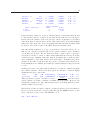
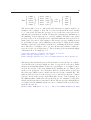
ASReml
User Guide
Release 3.0
July 2008
A R Gilmour
NSW Department of Primary Industries, Orange, Australia
B J Gogel
Department of Primary Industries, Brisbane, Australia
B R Cullis
NSW Department of Primary Industries, Wagga Wagga, Australia
R Thompson
Rothamsted Research, Harpenden, United Kingdom
ASReml User Guide Release 3.0
ASReml is a statistical package that fits linear mixed models using Residual
Maximum Likelihood (REML). It is a joint venture between the Biometrics Program of NSW Department of Primary Industries and the Biomathematics Unit
of Rothamsted Research. Statisticians in Britain and Australia have collaborated
in its development.
Main authors:
A. R. Gilmour, B. J. Gogel, B. R. Cullis and R. Thompson
Other contributors:
D. Butler, M. Cherry, D. Collins, G. Dutkowski, S. A. Harding, K. Haskard, A.
Kelly, S. G. Nielsen, A. Smith, A. P. Verbyla, S. J. Welham and I. M. S. White.
Author email addresses
[email protected]
[email protected]
[email protected]
[email protected]
Copyright Notice
c 2008, NSW Department of Primary Industries. All rights reserved.
Copyright °
Except as permitted under the Copyright Act 1968 (Commonwealth of Australia), no part of the publication may be reproduced by any process, electronic
or otherwise, without specific written permission of the copyright owner. Neither may information be stored electronically in any form whatever without such
permission.
Published by:
E-mail:
Website:
VSN International Ltd,
5 The Waterhouse,
Waterhouse Street,
Hemel Hempstead,
HP1 1ES, UK
[email protected]
http://www.vsni.co.uk/
The correct bibliographical reference for this document is:
Gilmour, A.R., Gogel, B.J., Cullis, B.R., and Thompson, R. 2008 ASReml User
Guide Release 3.0 VSN International Ltd, Hemel Hempstead, HP1 1ES, UK
ISBN 1-904375-23-5
1
0.1
Multi-environment trials
Revised 08
In this section, we explore some models that can be fitted to multi-environment
trials, in particular showing the application of factor analytic models.
A multi-environment trial is a series of experiments with treatments in common.
Our examples are drawn from field crops where the aim is to identify genotypes
which consistently yield well over a region in several seasons.
The traditional approach involved analysing the experiments separately, saving
the means, and then performing some analysis of the means. This approach
tends to ignore differences in experiment accuracy and to require each genotype
be tested in each experiment (limiting the experiments and/or genotypes that
can be considered together). The methods described in this section build on
spatial analysis, incorporate trial accuracy and allow for unbalance in genotype
representation. For further reading, see Smith et al. (2001, 2005).
Multi-environment trials have three basic forms. Early generation trials have few
sites and few replicates but many lines to compare. Current late-stage trials have
more 3-4 replicates, 10-15 sites and 30-50 entries of elite lines grown at most sites.
National analyses draw together results from multiple late-stage trials using results from several years and regions, many sites and many lines. We will consider
these three cases to discuss some features of ASReml. These analyses should
not be considered as definitive, typical or recommended as they demonstrate just
one approach. They are chosen to demonstrate syntactical issues, not statistical
issues.”
An early generation trial
Early stage multi-environment trials typically have many genotypes but limited
seed. Consequently, within site replication of test lines is low (1 or 2) so that lines
can be tested at more locations. Traditionally, grid plot designs have been used
where standard/reference/check lines are highly replicated using a systematic
grid but partial replicate designs are strongly advocated (Cullis et al. 2006).
This example involves 6 check lines and 330 test lines grown at three locations.
The first 2 locations were laid out in a 12 × 34 arrangement, 12 replicates of
each check line and 1 of each test line. The extra 6 plots were sown to a fill-in
variety which was also harvested. The third location was laid out in a 15 × 28
arrangement and had 15 replicates of each check line. The data file MET.DAT is
sorted row within column within site. The distributed data file has extra fields
2
we will ignore. The code for an initial combined analysis fitting a common random
test effect follows. This code incorporates the results from several preliminary
runs involving separate spatial analyses of each site ignoring test. These runs
suggested a random row term was required for site 3, col terms for all sites, AR1
was unnecessary for the col dimension of the R structure for site 3, and provided
the inital values inserted in the code. The !SECTION site qualifier allows ASReml
to check that the factor site does indeed correspond to the 3 sections in the R
structure. Notice in the 6 R structure lines that the field dimensions are explicitly
given in the first field, and the row/col in the second field enables ASReml to
sort/check the plots in field order.
Early Generation MultiEnvironment Trial
seq
col 15
# Actually 12 12 and 15 for the sites respectively
row 34
# Actually 34 34 and 28 for the sites respectively
chks 7
# 0 is fill-in, 1-6 are check lines, 7 is test line
test 336
# 0 is fill-in or check, 7-336 is test line
geno 337
# 1-6 are checks, 7-336 are test lines, 337 is fill-in
yld 1 !*.01
site 3
met.dat
!SECTION site
yld ~ site chk.site,
!r at(site,3).row .02 at(site).col .90 .40 .036 test
predict chk site
predict test site chks 7
site 2
12 col AR1 .1271
!S2=2.19 // 34 row AR1 .751
12 col AR1 .25
!S2=0.84 // 34 row AR1 .56
15 col ID
!S2=0.19 // 28 row AR1 .38
The LogL from this run is -314.262 and the parameter estimates follow.
- - - Results from analysis of yld - - Source
Residual
at(site,01).col
at(site,02).col
at(site,03).col
at(site,3).row
test
Variance[ 1]
Residual
Residual
Model terms
1236
1213
15
15
15
15
15
15
34
34
336
336
408
0
AR=AutoR
12
AR=AutoR
34
Gamma
0.622124
0.158966
0.483343E-01
0.235011E-01
0.103063
2.77228
0.195859
0.650554
Component
Comp/SE
0.622124
0.158966
0.483343E-01
0.235011E-01
0.103063
2.77228
0.195859
0.650554
1.45
1.40
1.85
2.77
7.02
8.80
3.64
16.80
% C
0
0
0
0
0
0
0
0
P
P
P
P
P
P
U
U
3
Variance[
Residual
Residual
Variance[
Residual
2]
3]
408
AR=AutoR
AR=AutoR
420
AR=AutoR
Source of Variation
8 site
9 chk.site
0
12
34
0
28
0.992656
0.286849
0.574471
0.120457
0.639281
0.992656
0.286849
0.574471
0.120457
0.639281
9.20
5.47
13.65
6.43
10.11
0
0
0
0
0
P
U
U
P
U
Wald F statistics
NumDF
F-incr
3
1230.64
20
11.36
Practioners have taken two views on whether check or reference lines should
be fitted as fixed effects, or just treated as random effects in the set of genotypes.
It may effect the variance of the test/genotype effects. Comparison of test lines
with check lines is easier if all are in the same random factor but this analysis
takes the former approach. Notice in passing that chk.site has 20 rather than
18 degrees of freedom because of the fill-in variety at the first 2 sites.
Our aim in this analysis is to get good predictions of test line effects. To do
this we can compare several models for the genetic variances and covariances
of test lines across sites. We are interested in the common effect of genotype
across sites, but also to know to what extent individual sites diverge from the
common genotype rankings. Our naive first model simply fits a common genetic
effect, primarily to show why this model is inadequate. It implies the genetic
variance is the same at all sites and the genetic correlation between sites is 1.
Both assumptions are unlikely given that the residual variances range from 0.12
to 2.77.
Adding site.test to the random model allows for a common covariance less than
the common variance. It increases the LogL from -314.262 to -310.879, highly
significant and gives components
test
336
336 0.867727E-01 0.867727E-01
5.46
0 P
site.test
1008
1008 0.440183E-01 0.440183E-01
2.62
0 P
0.08677
This represents a genetic correlation of 0.66 = 0.08677+0.04418
and an average
genetic variance of 0.1308 = 0.08677 + 0.04418, up from 0.1031. However, the
residual site variances are quite different (20 fold) so it is likely that the genetic
variances differ between sites.
Our next model therefore fits a common correlation but heterogeneous variances.
We drop test from the list of model terms and put the CORUH structure on the
site component of site.test. The ASReml code is
yld ~ site chk.site ,
4
!r at(site,3).row .02 at(site).col .90 .40 .036 site.test
site 2
1
12 col AR1 .1271
!S2=2.19 //34 row AR1 .751
12 col AR1 .25
!S2=0.84 //34 row AR1 .56
15 col ID
!S2=0.19
//28 row AR1 .38
site.test 2
site 0 coruh .66 .13 .13 .13 !GU
test
The LogL increases 22.4 (P<0.01) to -288.484 (P<0.01) and the components are
site.test
CORRelat
3
0.418611
0.418611
6.36
0 U
site.test
CORRelat
3
0.991289
0.991289
7.95
0 U
site.test
CORRelat
3
0.152347
0.152347
2.73
0 U
site.test
CORRelat
3
0.122776
0.122776
7.19
0 U
So the common correlation under this model is 0.42 (down from 0.66) and the
site variances are 0.99, 0.15 and 0.12 respectively; site 1 being particularly high.
This CORUH model would typically be the first model fitted. In this case there is
genetic variance at each site but sometimes that will not be the case.
Is the assumption of common correlation justified? Finally we fit an unstructured
model. This is often equivalent to an XFA1 model for 3 sites but with more sites,
the XFA1 model might be more parsimonious.
The G structure code is shown in the code
box. The resulting LogL is -286.824, an increase of 1.66 with 2 df (P>0.05). The initial
values were derived from the CORUH results, for
√
example, 0.16 = 0.42 ∗ (0.99 × 0.15).
site.test 2
site 0 US !GP
.99
.16 .15
.14 .06 .12
test
The fitted genetic variance matrix from the
unstructured model is:


.991 .157 .132


 .157 .072 .078 
.132 .078 .122
What next? Predicted values for the lines at each site are given in the .pvs file
by the predict statement
predict site test check 7 # Check 7 is the mean effect for test
Five site MET example
5
This second example is also an early generation trial but with more sites (5).
It demonstrates a set of five models typically fitted to current late-stage trials.
There were 330 genotypes replicated twice at each site except 7 plots were sown
to a fill in variety. Notice there is no separate coding of check-plot genotypes in
this example.
!RE !WORK 100 !NO !ARG 1 2 3 4 5 // !DOPART $1
Title: met.a307.
Plot * Block * Entry * Column * Row *
Genotype !A Site !A 5 Year !I Environment !A
yield
!*0.001
met307.csv !SKIP 1
!PART 1
!SECTION Site !Row Row !Col Column # generates standard spatial R structure
tab Block Col Row Gen ~ Site !stats # tabulates structural factors
yield ~ mu Site at(Site).lin(Row) at(Site).lin(Col) mv ,
# fixed model
!r at(Site).Row at(Site).Col at(Site).Block Site.Geno # random model
Site 2 1
# NB R structure is generated by ASReml so not here
Site.Geno 2
Site 0 CORUH
.5 5*.015
Geno
!PART 2 5
# Fits CORUH and US
!CONTINUE
yield ~ mu Site at(Site,1,2,4,5).lin(Row) at(Site,5).lin(Col) mv ,
!r at(Site,01,02,03,05).Row .003 .003 .0001 .0008 ,
at(Site).Col .06 .007 .002 .02 .001 ,
at(Site,2).Block .05 ,
Site.Geno
# Starting values inserted from PART 1
!PART 3 4
# Fits XFA1 and XFA2
!CONTINUE
yield ~ mu Site at(Site,1,2,4,5).lin(Row) at(Site,5).lin(Col) mv ,
!r at(Site,2).Block .05 at(Site,1,2,3,5).Row .003 .003 .0001 .0008 ,
at(Site).Col .06 .007 .002 .02 .001 ,
!PART 3
xfa(Site,1).Geno
!PART 4
xfa(Site,2).Geno
!PART 2 3 4 5
Site 2 1
55
5 AR1 0.5 !S2= 0.132 //
55
5 AR1 0.7 !S2= 0.22 //
55
5 AR1 0.74 !S2= 0.028 //
55
5 AR1 0.78 !S2= 0.22 //
55
5 AR1 0.68 !S2= 0.041 //
!PART 2
12
12
12
12
12
4
4
4
4
4
AR1
AR1
AR1
AR1
AR1
0.35
0.22
0.25
0.18
0.36
#Section
#Section
#Section
#Section
#Section
1
2
3
4
5
6
Site.Geno 2
Site 0 CORUH
# Starting values from PART 1
.62 .062 .10 .14 .16 .06
Geno
!PART 3
xfa(Site,1).Geno 2
xfa(Site,1) 0 XFA1
.018 .045 .004 .10 .012
.21 .24 .1 .22 .22
Geno
!PART 4
xfa(Site,2).Geno 2
xfa(Site,2) 0 XFA2
!G5P5P5P
.018 .045 .004 .10 .012
.21 .24 .1 .22 .22
5*.01
Geno
!PART 5
Site.Geno 2
Site 0 US !GP
0.5945E-01
0.4989E-01 0.1007
0.2145E-01 0.2443E-01 0.1443E-01
0.4640E-01 0.5285E-01 0.2272E-01 0.1503
0.4622E-01 0.5265E-01 0.2263E-01 0.4896E-01 0.6088E-01
Geno
Part 1 ended after 10 iterations with a LogL of 2563.4, not having quite converged.
Part 2 (starting from Part 1 estimates) converged in 7 iterations to LogL 2586.7.
These LogLs are not comparable because some fixed effects were dropped when
fitting part 2. Both these fitted the genetic variance matrix assuming equal
correlation among sites but different variances (CORUH).
Factor Analytic models provide a parsimonious approach generalising the covariance structure. Replacing CORUH with XFA1 in part 3 increased the LogL to
2611.71, a substantial gain. The XFA2 model in part 4 increased the LogL to
2621.57 after 10 iterations (not quite converged). Finally, fitting US in part 5
resulted in a LogL of 2622.06. This has only one more parameter than the XFA2
model which has 4 more free parameters than the XFA1 model. Consequently the
XFA2 model is the best fit.
In this case the unstructured variance matrix can be fitted but in general, especially with more than five sites, with high genetic correlations and with fewer
genotypes, the REML estimate of an unstructured variance matrix, if it can be
successfully estimated, may not be a positive definite matrix. The final genetic
7
0.10
5
2
−0.05
0.00
3
−0.15
−0.10
Second loading
0.05
1
4
0.10
0.15
0.20
0.25
0.30
0.35
First loading
Figure 1 loadings
variance matrix was
Covariance/Variance/Correlation Matrix UnStructured Site.Geno
0.05947 0.6092
0.7241
0.5229
0.7736
0.04755 0.1025
0.6013
0.5910
0.6717
0.02119 0.02310 0.01440 0.4829
0.7818
0.04943 0.07334 0.02247 0.1503
0.4438
0.04657 0.05308 0.02316 0.04247 0.06093
Recall, the average correlation from the CORUH model was 0.626.
It is convenient at this point to explore the XFA model which is akin to Principal
Components analysis. The underlying, latent variables are called factors. The
XFA1 model assumes a single factor, a set of genotype effects, usually called
genotype scores, that explain the covariance among sites. The XFA2 assumes
two genotype factors. The XFA2 model forms the across site variance matrix as
ΓΓ0 +Ψ with estimates from this example of


0.0172
0
0
0
0
0.186 0.088

 0.237 0.055 
0
0.043
0
0
0 








0
0
0.004
0
0  and Γ =  0.089 0.049 .
Ψ=





 0.347 −.171 
0
0
0
0.000
0 
0
0
0
0
0.008
0.188 0.133
The elements in the diagonal matrix Ψ are known as specific variances and represent the variation in genotype effects that is site specific (not associated with
8
the factors). The elements of Γ are the loadings for the two factors at the five
sites. They represent the regression of the genotype effects for each site on the
latent factors and plotting them maps the sites according to genetic similarity
highlighting that site 4 is most divergent (Figure 1).
The XFA2 variance matrix as presented in the .asr file (slightly reformated) is
Covariance/Variance/Correlation Matrix XFA xfa(Site,2).Geno
0.0594 0.6252 0.7120 0.5247 0.7762 0.7615 0.3627
0.0488 0.1024 0.6175 0.5883 0.6564 0.7391 0.1720
0.0208 0.0237 0.0144 0.4853 0.7850 0.7403 0.4089
0.0494 0.0727 0.0225 0.1490 0.4485 0.8983 -0.4394
0.0467 0.0518 0.0233 0.0427 0.0609 0.7628 0.5387
0.1857 0.2365 0.0889 0.3468 0.1883
1.000
0.000
0.0884 0.0550 0.0491 -0.1696 0.1330
0.000
1.000
The first 5 × 5 block is the variance matrix, directly comparable to the US matrix
displayed above, with derived correlations in the upper right triangle. The first
5 columns of the last 2 rows are the loadings, Γ0 , being the covariances of the
genotypes effects at the 5 sites with the latent factors. Similarly, the first 5 rows
of the last 2 columns are the correlations of the genotypes effects at the 5 sites
with the latent factors. The final 2 × 2 identity matrix relates to the two factors.
The .sln file also contains genotype effects for the five sites and two factors, that
is the genotype scores, as well as genotype effects for the 5 sites. For example
xfa(Site,2).Geno
xfa(Site,2).Geno
xfa(Site,2).Geno
xfa(Site,2).Geno
xfa(Site,2).Geno
xfa(Site,2).Geno
xfa(Site,2).Geno
BLA3071.VV5866
MTA3071.VV5866
PNA3071.VV5866
RSA3071.VV5866
WTA3071.VV5866
Factor_1.VV5866
Factor_2.VV5866
0.1006
0.1237
0.7299E-01
-0.3641
0.2089
-0.2370
1.661
0.9392E-01
0.1680
0.5347E-01
0.1638
0.8414E-01
0.3487
0.5551
˜
The
à genotype
! E-BLUPS for each site are calculated as Γs+ δ where s is the score
−.237
and δ˜ is a lack of fit residual (with variance given by Ψ). Note that
1.661
the residuals δ˜ are not explicitly returned by ASReml.
9




Thus 


0.1006
0.1237
0.0730
−0.3641
0.2089


 
 
 
=
 
 
0.186 0.088
0.237 0.055
0.089 0.049
0.347 −.171
0.188 0.133


Ã
! 
 −.237



+



1.661


−.0015
.0885
.0127
.0022
.0325




.


The factors will be close to orthogonal if the user has not applied explicit constraints to the loadings, or they can be rotated as shown in the next example
to be orthogonal. Plotting the genotype scores on the factor axes gives a two
dimensional representation of them. Plotting the loadings gives information on
the similarity of sites with respect to genotype ranking. Plotting both together
provides a biplot. Note that biplots are only useful when the factors plotted explain a large proportion of the variation. The average genotype ranking is given
by predicting genotype effects (BLUPs) at the average loadings (0.213, 0.031).
Stability of genotype performance is assessed by evaluating them at the extreme
sites. The choice of weights to use to produce an index upon which to rank genotypes is beyond our present purpose. The following predict statements simply
demonstrate how one might proceed.
predict Site Genotype # predicts each Genotype at each site.
predict Genotype !Average Site {1 1 1 0 1}/4
predict Genotype !AVE site 5*0 0.213 0.031 !ONLY xfa(Site,2).Geno # Average all
The first predict statement gives predicted means for each genotype at each site,
even though some genotypes might not have been grown at some sites. While
all sites are statistically distinct in this case, given Figure 1, one might be interested in the average of the most similar sites (excluding site 4). This is given
in the second prediction. Note that these first two predictions incorporate the
˜ The
Site×Genotype BLUPs and so include the the site specific residuals (δ).
third prediction is based on the genotype scores only and predicts the common
genotype effects at the average environment (the average of the loadings). Note
the !ONLY qualifier. Without it, the predictions are not estimable because they
˜ are
include the mu term but note Site fixed effects. The site specific residuals (δ)
not included in the ASReml output but can be calculated with a predict statement like (for site 4)
predict Geno !AVE Site 0 0 0 1 0 -.347 0.171 !ONLY xfa(Site,2).Geno
10
Meta analysis of trial means
When it comes to later stages of selection, it is desirable to include as many
experiments as possible representing different locations and seasons when comparing genotypes. This will commonly be over 30 experiments after 3 years of
evaluation, and could easily be as many as 100 trials. Furthermore, few genotypes
will be represented at all sites. The combined analysis of experiments at the plot
level discussed in the previous subsection is therefore not always feasible.
We describe a two step approach. First, each experiment is analysed separately
under a spatial model and predicted genotype means are produced along with a
set of weights (see !TWOSTAGEWEIGHTS on page ??). Ideally these should be stored
in a database so that they can be conveniently retrieved later for subsequent
analysis. We also store the site mean yield and the residual variance along with
details of the spatial model fitted.
For this example, we have extracted 2019 predicted lupin yields from the data
base, with their weights. They represent 203 genotypes and 87 experiments
conducted in 3 regions over 5 years. The yields range from 0.09300 to 5.613 with
an average of 1.732. The experiment variances range 0.00037 to 0.04671 with an
average of 0.02491. Note that the weights have been scaled by this average value
(via transformation and back again in the model) so that variances have their
natural scale. Following is code that fits 5 models to this data.
!WORK 1 !NO !CONTINUE !RENAME !ARG 11 1 2
// !DOPART $1
Title: ALBUS_2stage.
#trial,year,region,variety,yield,rep,weight,ems
#KFA02BURU,2002,NSW,KIEV-MUTANT,0.873,3,2136.562,0.0010000
trial !A year !I region !A variety !A
yield rep * weight
!*0.025 ems
ALBUS.csv
!SKIP 1
!MAXIT 40
!PART 11
# Initial Model - Uniform correlation, heterogenous variance
#Shows trials 51 and 85 have minimal variance: fix .0001
yield !wt=weight ~ mu trial !r trial.variety
# LogL 2783.33
1 1 1
0 !S2==0.025
trial.variety 2
trial 0 CORUH .1
87*.1
variety
!PART 1 2 3 4
# Sequence of Factor Analytic models
# XFA1 LogL 2911.52
increase of 128.18
# XFA2 LogL 3039.34 then 3050.38 increase of 138.86
11
# XFA3 LogL 3155.65
# XFA4 LogL 3201.99
then 3158
then drift
increase of 105
increase of 44
yield !wt=weight ~ mu trial !r xfa(trial,$1).var
1 1 1
0 !S2==0.025
xfa(trial,$1).var 2
xfa(trial 0 XFA$1
!GP
50*.01 .0001 33*.01 .0001 2*.01
87*.07 87*.07
87*.07 87*.07
variety
The equal correlation model is fitted first in part 11. After 40 iterations, it had
converged with a LogL of 2783.3 with an average genetic correlation of 0.55.
Continuing with XFA1 in part 1, the LogL increases to 2911.52 in another 40 iterations, with 9 specific variances at 0.0. The factor explains 56% of the genotype
variation. Again, using !CONTINUE to start with the XFA1 values, part 2 fits an
XFA2 model. After 40 iterations, the LogL had reached 3039 and another 40 iterations increased it to 3050.4, with 23 of the 87 specific variances fixed at 0.0. The
second factor explains a further 18% of the genotype variation. The parameters
were still changing slightly but this provides two factors and permits a biplot of
genotypes and experiments to be formed.
XFA models with two or more factors are often difficult to fit. The main strategy
for fitting these models is getting better starting values which is why these 5
models are fitted in sequence and using !CONTINUE. The !AILOAD f qualifier
may also help. It is set by default when XFAk model parameters are initialized
using !CONTINUE from a previous XFA model fit with k − 1 factors. The strategy
followed, when the user does not supply explicit constraints and !AILOAD f is
set, has three stages. The first stage is to hold the first k − 1 factor loadings
fixed for a few iterations, estimating the loadings for the kth factor and the
specific variances. The second stage is to estimate two factors and the specific
variances until iteration f before updating all factors simultaneously in the third
stage. There is also an automatic procedure which shrinks the AI updates for
the loadings as a set if as a set they appear relatively large.
Moving from XFA2 to XFA3, the LogL increased 105 (3050 to 3155) with 74 extra
parameters (87 loadings less 2 constraints on loadings and 11 more specific variances fixed at 0.0) which is about twice the 5% critical value. However this model
has trouble converging, a problem we are still investigating. The LogL increased
12
nicely to 3155 in 40 iterations. Continuing, it rose to 3157, drifted to 3144, rose
again to 3158 and dropped away to 3154. A pragmatic option is to rerun the job
using !MAXIT to stop at the iteration with the highest LogL and accept that as
the solution.
Proceeding to XFA4 is probably ambitious. Starting from the 3155 XFA3 solution
and using the default !AILOAD f strategy, the LogL increases to 3201 briefly but
quickly starts decreasing. In another run, the first 3 loadings were held at their
XFA3 values until approximate convergence at LogL of 3209. Then continuing
with using !AILOADINGS 20, the LogL rose to around 3235 (with 51 specific
variance at 0.0) before drifting away. This is an increase of 80 which for 76 (=87
- 3 - 8) extra parameters is close to the 5% critical value.
The interpretation of results from a factor analytic model is not easy, but is similar
to interpreting results from a principal components analysis. First, users are referred to the section of the .res file headed DISPLAY of variance partitioning
for XFA structure in ... which lists the specific variance and loadings as a
table with a figure (see page ??). Further investigation must be done outside of
ASReml using the variance parameters and the fitted effects.