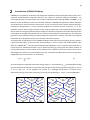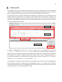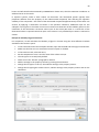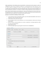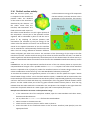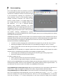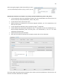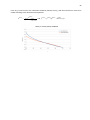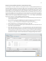
1
1 COSMOthermX A Graphical User Interface to the COSMOtherm Program User Guide Version C30_1501 COSMOlogic GmbH & Co. KG Imbacher Weg 46, D-51379 Leverkusen, Germany 2 Table of Contents List of Examples............................................................................................................................................. 4 Abbreviations ................................................................................................................................................ 5 A Quick Start.......................................................................................................................................... 6 1.1 1.2 1.3 Compounds.................................................................................................................................... 6 Property input ............................................................................................................................... 8 Workplace...................................................................................................................................... 9 Introduction: COSMO-RS theory ......................................................................................................... 10 COSMOtherm and COSMOthermX ...................................................................................................... 12 3.1 3.2 3.3 3.4 3.5 3.6 3.7 3.8 Quality levels and parameterizations .......................................................................................... 12 Flowchart of a property calculation with COSMOthermX ........................................................... 14 The main window ........................................................................................................................ 15 Job list .......................................................................................................................................... 19 The Workplace Window .............................................................................................................. 20 Preferences .................................................................................................................................. 20 Calculation options and Property options ................................................................................... 22 Input and Output Files ................................................................................................................. 29 Compounds ......................................................................................................................................... 30 4.1 4.2 4.3 4.4 4.5 Compound selection.................................................................................................................... 30 The compounds context menu .................................................................................................... 31 Selecting compounds from databases ........................................................................................ 34 New Molecules ............................................................................................................................ 35 Conformers .................................................................................................................................. 38 4.6 4.7 Visualization of -surfaces, -profiles, and -potentials ............................................................ 39 Using COSMOview ....................................................................................................................... 40 Property input ..................................................................................................................................... 42 5.1 5.2 5.3 5.4 5.5 5.6 5.7 5.8 5.9 5.10 Phase definition ........................................................................................................................... 43 Mixture: Calculation of compound properties in mixture .......................................................... 44 Vapor pressure ............................................................................................................................ 44 Boiling point................................................................................................................................. 46 Activity coefficient calculation .................................................................................................... 46 Henry law coefficient calculation ................................................................................................ 47 Gas solubility ............................................................................................................................... 48 Solubility ...................................................................................................................................... 48 Solvent screening ........................................................................................................................ 51 Salt solubility ............................................................................................................................... 55 3 5.11 5.12 5.13 5.14 5.15 5.16 5.17 5.18 5.19 Salt solubility screening ............................................................................................................... 58 Partition coefficient calculation (log P / log D) ............................................................................ 59 Calculation of pKA ....................................................................................................................... 61 Vapor liquid-equilibria (VLE) and liquid-liquid equilibria (LLE) .................................................... 63 Solid liquid equilibria ................................................................................................................... 66 FlatSurf: surface activity .............................................................................................................. 69 Interfacial Tension ....................................................................................................................... 71 Density ......................................................................................................................................... 72 Viscosity ....................................................................................................................................... 73 5.20 5.21 5.22 5.23 5.24 5.25 5.26 5.27 5.28 The -moment approach and QSPR calculations ........................................................................ 73 Similarity ...................................................................................................................................... 74 Liquid extraction .......................................................................................................................... 75 Reaction ....................................................................................................................................... 77 Cocrystal screening with COSMOthermX .................................................................................... 80 COSMOmeso: Flory-Huggins and DPD Parameter with COSMO-RS ............................................ 81 Ionic Liquid Screening .................................................................................................................. 82 Ionic Liquid Properties ................................................................................................................. 82 Environmental / Safety ................................................................................................................ 83 COSMO files and databases ................................................................................................................ 84 6.1 6.2 Embedding a COSMObase ........................................................................................................... 85 The COSMObase Editor ............................................................................................................... 85 Atom weighting ................................................................................................................................... 89 Appendix A: Systems with Ionic Liquid (IL) compounds ............................................................................. 91 Appendix B: Treatment of Polymers ........................................................................................................... 96 Index............................................................................................................................................................ 99 4 List of Examples Example 1: Glycofurol ................................................................................................................................ 38 Example 2: COSMO charge surface visualization, -profile and -potential. ........................................... 39 Example 3: Calculation of a vapor pressure curve ..................................................................................... 45 Example 4: Calculate the activity coefficient of aspirin in water............................................................... 46 Example 5: Gas solubility of methane in water ......................................................................................... 48 Example 6: Solubility of glycol in hexane ................................................................................................... 50 Example 7: Estimated solubility improvement of the cocrystal systems carbamazepine – niacinamide and carbamazepine – oxalic acid in water ................................................................................................ 55 Example 8: Prediction of the solubility of NaCl in several solvents ........................................................... 59 Example 9: Prediction of octanol / water partition coefficients................................................................ 60 Example 10: Calculation of the aqueous pKA of pyrrolidine ..................................................................... 61 Example 11: Calculate the solubility of aniline in water ............................................................................ 65 Example 12: Solid-liquid equilibrium curve of toluene and ethylbenzene ................................................ 67 Example 13: Calculate the air-water surface partition energy .................................................................. 69 Example 14: Interfacial Tension for a binary water / heptane system ...................................................... 71 Example 15: Liquid density and liquid molar volume of pure compounds ............................................... 72 Example 16: Three-phase equilibrium between water, hexane, and [bmim+][pf6-] with an additional solute ................................................................................................................................................. 76 Example 17: Solvent choice for a simple ester reaction ............................................................................ 78 Example 18: Cocrystal formation in a 1:1 mixture of 4-pyridinecarbonitrile and 1,3,5-trihydroxybenzene ........................................................................................................................................................... 80 Example 19: Calculate the infinite dilution activity coefficients of water in IL (1-butyl-3-methylimidazolium_cation + PF6_anion)...................................................................................................... 93 Example 20: Calculate a LLE of water in IL (1-butyl-3-methyl-imidazolium_cation + PF6_anion) ............ 94 Example 21: Activity Coefficient Calculation in a Macromolecular Solvent .............................................. 97 5 Abbreviations 2D: 3D: AM1: BP-SVP / BP-TZVP: CAS-Number: COSMO: COSMO-RS: DB: DFT: HB: IL: LFER: LLE: MW: QC / QM: QSPR: (sigma): SLE: SMILES: SMS: VLE: Two dimensional Three dimensional A semiempirical quantum chemical method Becke-Perdew1, 2, 3 (BP) functional for density functional theory calculations with a split valence plus polarization function (SVP) or triple valence plus polarization function (TZVP) basis set. The necessary parameterization file does always correspond to one functional and basis set. The term “BP-TZVP parameterization” is thus sometimes used and refers to the COSMOtherm parameterization not the basis set specification. The Chemical Abstracts Services registration number is a unique identifier for compounds. COnductor like Screening MOdel COnductor like Screening MOdel for Real Solvents Database, usually used for the COSMOtherm compound databases. Density Functional Theory: A quantum chemical theory used in several software packages for molecular or lattice calculations. Hydrogen Bond Ionic Liquid Linear Free Energy Relationship Liquid Liquid Equilibrium Molar Weight Quantum Chemical / Quantum Mechanical Quantitative Structure Property Relationship, also QSAR (A = activity) The COSMO screening charge Solid Liquid Equilibrium Simplified Molecular Input Line Entry Specification, notation to describe molecules e.g. methane is “C” ethane is “CC” and ethanol is “CCO” Sigma Match Similarity Vapor Liquid Equilibrium 6 A Quick Start This chapter is intended as a quickstart guide and addresses the basic steps needed to start a COSMOtherm calculation. All steps are described in more detail in separate chapters. The general procedure for a COSMOtherm calculation involves two steps: compound selection and property input. The Graphical User Interface has panels and dialogues for these steps. The most customary procedures are described in this chapter. 1.1 Compounds A COSMOtherm calculation requires screening charge distributions of the molecules involved in the system in question. The screening charge distribution can be taken from the screening charge surface of the molecule, as calculated in a quantum chemical COSMO calculation. The result of the COSMO calculation is stored in a COSMO file with the extension .cosmo or .ccf. In principle, COSMO files can be generated on almost any quantum chemical level. For applications in standard chemical and engineering thermodynamics, we recommend to use the TZVP or the TZVPD-FINE levels. Both levels are based on molecular structures retrieved from DFT calculations, but the TZVPD-FINE level involves additional QM energy calculations with the TZVPD basis set. Generally, COSMOtherm calculations on the TZVP level are faster, while the TZVPD-FINE level gives slightly better results. Depending on the number of compounds involved, the computer power available, and the accuracy required, other levels can be better suited for other purposes. COSMOtherm reads the compound information from the COSMO file(s) of the compound and transforms the screening charge surface into a screening charge distribution, called -profile. Information about the molecular structure is generally not required and is discarded. Because -profiles for conformers of one compound may differ depending on the molecular structure, conformers have to be calculated individually. If COSMO files of several conformers exist for a compound, they will be combined into a single compound. For detailed information on the selection of conformers for COSMO calculations and on the conformer treatment in COSMOtherm refer to section 4.5. On start-up, there are two tabs in a COSMOthermX workplace window: COMPOUNDS and PROPERTIES. compound list and database access 7 Compounds can be selected from the COMPOUNDS tab. There are two ways to do this: from one of the databases, using one of the buttons labeled SVP, TZVP, DMOL3, or TZVPD-FINE. from the FILE MANAGER To select a compound from one of the databases, click on the corresponding database button, e.g. TZVP, and open the database dialog which lists all available compounds. The database dialog has several functionalities: By default, compounds from all embedded databases of the selected level will be listed. Databases can be selected or deselected using the checkboxes in the SELECT DBS TO SEARCH line. A mouse-over will show the location of the database directory. Compounds can be tagged for selection by checking the box in the first column. All tagged compounds will be transferred to the compound section in the main window when the GET SELECTION button is pressed. Double-clicking a compound will also transfer the compound to the compound section in the main window. Clicking on a column header will sort the databases according to that column. By default, all conformers of a compound will be selected. However, the box in the USE CONF. column can be untagged: then only the lowest-energy conformer will be transferred to the compound section. In case a specific conformer other than the lowest energy conformer is needed, first select the complete conformer set. Then delete the unwanted conformers from the compound section by highlighting them and pressing the "Del" key. Database tables are searchable. Enter a search string (name, formula, CAS-Number, smiles code) and process the search by pressing SEARCH, or SEARCH SMILES. To select compounds from a place in your directory tree, click on the FILE MANAGER button. Go to the directory where the COSMO files of the required compounds are located and highlight the files. Several files can be highlighted by keeping the "Ctrl" key pressed while clicking on the file names. To transfer the 8 highlighted COSMO files to the compound section, press the SELECT button on the left side of the FILE MANAGER window. In case the parameterization is not discernible from the COSMO file you will be asked to choose a parameterization to fit the selected files. Make sure that you use an adequate parameterization, i.e. the one corresponding to the DFT functional and basis set used in the quantum chemical COSMO calculation. Selected compounds are listed in the compound section. For detailed information on additional options for the compound list please refer to chapter 4. 1.2 Property input Once the compounds are selected, change to the PROPERTIES tab and select the property you want to calculate. Each property panel comprises fields for the adjustable settings. Settings required for all property calculations are the temperature and the composition of the system. The composition of the system can be set in three ways: if it consists of one compound only, just tick the box in the PURE column. If the system is composed of several compounds, the mole or mass fraction numbers can be set compound-wise in the corresponding fields. Alternatively, the sliders in the compound lines can be used 9 to set the mole or mass fractions. Depending on the property, other input, e.g. the composition of a second phase, might be required. When all parameters have been set, press the ADD button at the bottom of the input preparation panel to finish the property input. It is possible to prepare input for several COSMOtherm calculations in a single job. To run a job, press the RUN button. Jobs can be saved and run with jobnames. If a jobname is not used, jobs are run as temporary jobs, and input and output files are deleted when COSMOthermX is closed. Job input files can also be saved permanently before running with the SAVE AS button. temperature and phase composition 1.3 Workplace Starting with version C30_1401 it is possible to open several workplace window inside the main frame. Several jobs can be set up and run at the same time. When a job has finished, calculation results are displayed in separate tabs in the workplace window. To open a new workplace, use NEW JOB from the FILE menu or simply click on the shortcut icon from the toolbar. If the view is changed to CLASSIC STYLE, the Job list is minimized into the toolbar. The workplace window is enlarged to cover the main window and the COMPOUNDS and PROPERTIES tabs are arranged side by side. 10 Introduction: COSMO-RS theory COSMO-RS is a predictive method for thermodynamic equilibria of fluids and liquid mixtures that uses a statistical thermodynamics approach based on the results of quantum chemical calculations. The underlying quantum chemical model, the so called “COnductor-like Screening MOdel” (COSMO)4, is an efficient variant of dielectric continuum solvation methods. In COSMO calculations the solute molecules are calculated in a virtual conductor environment. In such an environment the solute molecule induces a polarization charge density on the interface between the molecule and the conductor, i.e. on the molecular surface. These charges act back on the solute and generate a more polarized electron density than in vacuum. During the quantum chemical (QC) self-consistency algorithm, the solute molecule is thus converged to its energetically optimal state in a conductor with respect to electron density. The molecular geometry can be optimized using the same methods for calculations in vacuum. The time consuming QC calculation has to be performed only once for each molecule of interest. The polarization charge density of the COSMO calculation (also called screening charge density), which is a good local descriptor of the molecular surface polarity, is used to extent the model towards “Real Solvents” (COSMO-RS)5, 6. The (3D) polarization density distribution on the surface of each molecule i is converted into a distribution-function, the so called -profile pi(), which gives the relative amount of surface with polarity on the surface of the molecule. The -profile for the entire solvent of interest S, which might be a mixture of several compounds, pS() can be built by adding the pi() of the components weighted by their mole fraction xi in the mixture. pS x i p i (1) iS The most important molecular interaction energy modes, i.e. electrostatics (Emisfit) and hydrogen bonding (EHB) are described as functions of the polarization charges of two interacting surface segments and ' or acceptor and donor , if the segments are located on a hydrogen bond donor or acceptor atom. Electrostatic energy arises from the misfit of screening charge densities and ', as illustrated below. O H H H H O O H H H H O O H O H H ’ - ++ + O O H H O C H H O H O O H H H H O O O >>0 ’<<0 H O O H H O H H H H H O H O C H H H O O 11 The less specific van der Waals (EvdW) interactions are taken into account in a slightly more approximate way. E misfit ( , ' ) aeff ' 2 ( ' )2 (2) E HB aeff cHB min0 ; min0 ; donor HB max0 ; acceptor - HB (3) EvdW aeff vdW 'vdW (4) Eqs. 2-4 contain five adjustable parameters, an interaction parameter ’, the effective contact area aeff, the hydrogen bond strength cHB, the threshold for hydrogen bonding HB, and the element specific vdW interaction parameter vdW. In order to take the temperature dependency of EHB and EvdW into account, temperature dependent factors are applied, each with one adjustable parameter.7 The transition from microscopic molecular surface charge interactions to macroscopic thermodynamic properties of mixtures is possible with a statistical thermodynamic procedure. The molecular interactions in the solvent are fully described by pS(), and the chemical potential of the surface segments can be calculated solving a coupled set of non-linear equations. S a eff RT S ' E misfit , ' E HB , 'd ' ln p S 'exp a eff RT (5) The -potential S() is a measure for the affinity of the system S to a surface of polarity . The vdW energy, which does not appear in Eq. (5), is added to the reference energy in solution (energy of the COSMO calculation). The chemical potential of compound i in the system S (the solvent) can now be calculated by integration of S() over the surface of the compound. Si Ci ,S p i S d (6) To take into account size and shape differences of the molecules in the system an additional combinatorial term, iC,S, which depends on the area and volume of all compounds in the mixture and three adjustable parameters is added. For information on the exact expression for the combinatorial term refer to the COSMOtherm Reference Manual. The chemical potential can be used to calculate a wide variety of thermodynamic properties, e.g. the activity coefficient: Si ii RT Si exp (7) where iS is the chemical potential in the solvent S, and ii is the chemical potential of the pure compound i. For a more detailed introduction to COSMO and COSMO-RS, refer to the COSMOtherm Reference Manual and the cited literature. 12 COSMOtherm and COSMOthermX COSMOtherm is a command line/file driven program which can be run directly from a UNIX or DOS shell. It allows for the calculation of any solvent or solvent mixture and solute or solute system at variable temperature and pressure. COSMOtherm uses the chemical potentials derived from COSMO-RS theory to compute all kinds of equilibrium thermodynamic properties or derived quantities, e.g.: Vapor pressure Free energy of solvation Activity coefficients Partition coefficients Solubility and solid-liquid equilibria (SLE). Liquid-liquid equilibrium (LLE) and vapor-liquid equilibrium (VLE) Phase diagrams, azeotropes, miscibility gaps, excess enthalpies and excess free energies pKA of acids and bases Various QSPR models Reaction constants Liquid extraction equilibria COSMOthermX is a Graphical User Interface to the COSMOtherm command line program. It allows for the interactive use of the COSMOtherm program, i.e. selection of compounds, preparation of property input, program runs and display of calculation results. 3.1 Quality levels and parameterizations The input for the compounds is read from the COSMO files, identified by the extensions .cosmo or .ccf, which are result files from quantum chemical COSMO calculations. COSMOtherm extracts the relevant information directly from the COSMO files. The compressed COSMO files (.ccf) use significantly less disk space than conventional COSMO files. At least one COSMO file or compressed COSMO file has to be selected as compound input. Note that COSMO file names with blanks are not allowed by COSMOthermX. Because the quality, accuracy, and systematic errors of the electrostatics resulting from the underlying COSMO calculations depend on the quantum chemical method as well as on the basis set, COSMOtherm needs a special parameterization for each method / basis set combination. All of these parameterizations are based on molecular structures quantum chemically optimized at the given method / basis set level. COSMO files shipped with COSMOtherm are available on various quantum chemical levels. Recommendations for which method to use depend upon the required quality and the later usage of the predictions. The application of COSMOtherm in chemical and engineering thermodynamics (e.g. prediction of binary VLE or LLE data, activity coefficients in solution or vapor pressures) typically requires high quality of property predictions of mixtures of small to medium sized molecules (up to 25 non-Hydrogen atoms). The recommended quantum chemical method for such a problem is a full TURBOMOLE BP-RI-DFT COSMO optimization of the molecular structure using the large TZVP basis set8, in the following denoted BP-TZVP, and the corresponding parameter file BP_TZVP_C30_1501.ctd. A similar quality can be reached with 13 the DMOL3 program package using full COSMO and gas phase geometry optimization with the PBE DFT functional and the numerical DNP basis set and the corresponding parameter file DMOL3_PBE_C30_1501.ctd in COSMOtherm. The BP-TZVPD-FINE level, introduced in 2012, is based on a Turbomole BP-RI-DFT COSMO single point calculation with TZVPD basis set on top of an optimized BP/TZVP/COSMO geometry. The COSMO single point calculation is using the TZVPD basis set with diffuse basis functions and a novel type of molecular surface cavity construction (fine grid marching tetrahedron cavity, FINE9), which creates a COSMO surface whose segments are more uniform and evenly distributed compared to the standard COSMO cavity. The gas phase energy files of this level are optimized on Turbomole BP-RI-DFT level with TZVP basis set, followed by a single point BP-RI-DFT calculation with the TZVPD basis set. The associated BP_TZVPD_FINE_C30_1501.ctd parameter set additionally incorporates the HB2012 hydrogen bonding term and a novel van der Waals dispersion term based on the “D3” method of Grimme et al.10, which shows improved thermodynamic property prediction results for compound classes where the classical COSMO-RS hydrogen bonding term showed weaknesses, e.g. with secondary and tertiary aliphatic amines and polyether compounds. In addition, the wider realm of organic liquid and gas phase thermodynamics is predicted with the same quality or slightly better as the standard BP-TZVP-COSMO and DMOL3_PBE methods. Hence the BP-TZVPD-FINE level in combination with the BP_TZVPD_FINE_C30_1501.ctd parameterization is considered to be the “best quality” calculation method currently available. Until further experience is gained, this level of theory and parameterization are provided in an “as is” state. Nevertheless, COSMOtherm users should feel encouraged to try this level: it probably fits their special demands in property prediction better than the standard levels BP-TZVPCOSMO and DMOL3-PBE, in particular if the mentioned compound classes are involved. Screening a large number of compounds, e.g. prediction of solubility of compounds in various solvents, typically requires a predictive quality that is somewhat lower than for chemical engineering applications. The molecules involved are often larger (>100 atoms) and an overall large number of compounds has to be computed by quantum chemistry. Thus a compromise between computational demands and quality of the predictions has to be made: A very good compromise is the optimization of molecular geometry on the computationally very cheap semiempirical MOPAC AM1-COSMO level11 with a subsequent single point COSMO calculation on Turbomole BP-RI-DFT COSMO level using the small SVP basis set. This method is named BP-SVP-AM1 in the following, and the corresponding parameterization is available in the BP_SVP_AM1_C30_1501.ctd parameter file. For more information on available quantum chemical levels and parameterizations refer to the COSMOtherm Reference Manual, section 3. Please note that starting with version C3.0 Release 14.01 of the COSMOtherm program, the unit conversions and fundamental physical constants used in the COSMOtherm parameterizations (Avogadro constant NA, Boltzmann constant k, Elementary charge e, Electron mass me, Planck constant h, and Electric constant e0) were updated according to the latest NIST/CODATA recommendations12. In older parameterization files, the original values of the physical constants and unit conversions have been retained, to ensure downward compatibility of the predictions with these parameter sets. 14 3.2 Flowchart of a property calculation with COSMOthermX COSMOthermX external Start Select compounds from the Databases or the File Manager Add compounds to database Found all compounds ? No Yes TURBOMOLE Select settings for property calculations Add Another property? No Run Use the New Molecule Wizard to generate COSMO files and/or gas phase structures. Yes 15 3.3 The main window In the default view, the main window has a Job List frame on the left and space for several resizable workplace frames in the major section. At startup, a workplace window has a panel for the compound list (COMPOUNDS) with database access and another panel for property input preparation (PROPERTIES). Main menu and shortcuts Job list Workplace window: Compound list with database access Property panels for input preparation The COSMOthermX main window has several menus, some of them also available from shortcut icons in the toolbar: File: NEW JOB: Create a new input file in a new workplace window. OPEN JOB: Open an existing input file from a file browser dialog. Select a file from the directory or type the filename into the “File name” text field and press “Open”. SAVE: Save the input file to the current directory with the actual name. SAVE AS…: Choose a directory and a name for the input file to be saved. CLOSE JOB: The job selected from the job list is removed from the list. All input and output files of the job are kept. DELETE JOB: The job selected from the job list will be deleted, together with all input and output files of the job. QUIT: Exit the program. Edit: COPY: Copy text from a text editor window or compounds from a workplace. 16 PASTE: Paste selected text to a text area, respectively compounds to a workplace. EDIT INPUT FILE: Open the actual input file in a text editor window. The input file can be changed manually, e.g. for additional input in the compound lines (further information: COSMOtherm Reference Manual).The input file can be saved or COSMOtherm can be run. Note that not all changes can be read in when the input file is re-opened with COSMOthermX. OPEN WORKPLACE: Open a new workplace window. Compounds: SVP: open database index files of the BP-SVP-AM1 level of theory in tabulated form. TZVP: open database index files of the BP-TZVP level of theory in tabulated form. TZVPD-FINE: open database index files of the BP-TZVPD-FINE level of theory in tabulated form. DMOL3: open database index files of the DMOL3-PBE level of theory in tabulated form. SEARCH IN ALL DB: Search a compound in all databases that are listed in the EXTRAS/ GENERAL SETTINGS DATABASES pane, irrespective of the parameterization which the DBs are linked to. NEW MOLECULE: This option allows for searching for a compound by name, CAS-Number, SMILES or structure. It also offers the possibility to generate a complete new structure with TURBOMOLE (if installed). FILE MANAGER: Opens a compound from an arbitrary directory. SAVE COMPLETE COMPOUND LIST: With this option it is possible to save the complete compound list to a file for later use. The concentrations are also saved. To save only the selected compounds to a list use the SAVE TO COMPOUND LIST option from the compound list context menu has to be used. OPEN COMPOUND LIST: A list of previously saved compounds can be loaded with this option. The saved concentrations of the compounds will also be loaded but not automatically applied. SET DEFAULT CONCENTRATIONS: Apply the saved list concentrations after loading a compound list. The saved concentrations of the compounds will not be applied automatically when a list is opened. Run: RUN: The actual input file is saved automatically with the current file name and COSMOtherm is run. RUN (EXTERNAL) INPUT: A COSMOtherm calculation can be run with an external input file, without opening it in the GUI. Any valid COSMOtherm input file can be run. 17 STOP RUNNING JOBS: Running COSMOtherm Jobs will be stopped. Result: OPEN OUTPUT FILE: Select a COSMOtherm output file from a directory or type the filename into the “File name” text field and press “Open”. OPEN TABLE FILE: Select a COSMOtherm table file from a directory or type the filename into the “File name” text field and press “Open”. OPEN COSMOMIC FILE: Select a COSMOmic file from a directory or type the filename into the “File name” text field and press “Open”. SHOW RESULTS: Output and table files of the active job will be opened in separate tabs of the workplace window. VIEW AS .XLS: The table file of the active job will be opened in a spreadsheet program (if available) SAVE AS .XLS(X): The table file of the active job will be saved in MS Excel format. SHOW EXTENDED OUTPUT: By default, only the summary table with a truncated number of columns is displayed in a table editor. With this option, the complete results table will be displayed. HIDE EXTENDED OUTPUT: The summary table will be displayed. The number of columns is truncated to allow for a concise representation of results. SAVE OUTPUT FILE AS: The output file can be saved in text format. Extras: CALCULATION OPTIONS: A panel with general calculation options, including options for gas phase energy input, units, COSMOtherm output print options, additional output files and program control. For a detailed description see below. PROPERTY OPTIONS: A panel with special options applied to certain property calculation only when specified. For individual property calculations, print options for output and table files can be set, program control settings can be changed, and compound specific options can be set. Property Options are used to apply options to a certain property calculation only. With these options it is possible to use different options in a single COSMOtherm run. Property Options will only be used if the USE PROPERTY OPTIONS checkbox is activated in the corresponding property panel. If several mixtures or properties are calculated in a single run, the Property Options have to be activated each time the property settings are transferred to the property selection window, otherwise they will not be used for the respective property calculation. For a detailed description see below. VIEWER SETTINGS: Change atom / bond color, show or hide label, change sphere / cylinder smoothness and so on. 18 PREFERENCES: Opens the PREFERENCES dialog where some settings are already specified: Paths for the COSMOtherm executable and the CTDATA directory of the COSMOtherm installation are set, and the parameter files for the quantum chemical levels are specified. Additionally, you can set paths for the Adobe Acrobat Reader and a web browser. If you intend to use COSMO metafiles (extension .mcos) for the fragment approach, you should also specify the fragment directory. When the path for the QSPR property directory is set QSPR coefficient files (extension .prop) can be read from there. For details see below. DATABASES: Opens the PREFERENCES dialog with the COMPOUNDS tab. The databases that come with the COSMOtherm release are specified here. Additional databases can be added with ADD DATABASES. For detailed information on adding your own databases, refer to the section “COSMO files and Databases”. IMPORT SETTINGS: Settings from other COSMOthermX versions can be imported. Tools: COSMOVIEW: Opens the COSMOview tool which allows for the visualization of .wrl files generated by COSMOtherm. For more information, please refer to the section “Using COSMOview”. COSMOWEIGHT: Opens the COSMOweight tool. For information on atom weighting and the COSMOweight tool, please refer to the section “Atom Weighting”. COSMOBASE EDITOR: Opens the COSMObase Editor which allows for creating and administration databases of compound COSMO, gas phase energy and Vapor Pressure / Property files. For details, refer to the section “The COSMObase Editor”. View: CLASSIC STYLE: Arrange frames similarly to the view in previous COSMOthermX versions (up to version C30_1301). The Compounds panel is moved internally to a separate frame on the left side of the Properties panel. The Job list is disconnected from the main frame. DEFAULT STYLE: Restore the default arrangement of frames in the main window. The Job list is expanded in the main window and the Compounds and Properties panels are arranged in tabs in the workplace window. LAPTOP STYLE: The Job list is disconnected from the main frame and the workplace window is enlarged to fill the complete main frame. TILE WINDOWS: Arrange workplace windows in tiles in the main window. CASCADE WINDOWS: Arrange workplace windows in a cascade in the main window. 19 License: IMPORT LICENSE: Opens a file browser for the selection of a license file. Use to change from demo mode to full COSMOtherm. CHECK LICENSE: Display license information in a text viewer window. Help: PHYSICAL CONSTANTS: Displays information about some physical constants and conversion factors. OPEN EXAMPLE: Opens a file browser in the COSMOtherm Examples subdirectory. Example input files can be opened and run in COSMOthermX. COSMOTHERM MANUAL: Open the COSMOtherm Reference Manual with the Adobe Acrobat Reader. COSMOTHERMX USER GUIDE: Open the COSMOthermX User Guide (this document) with the Adobe Acrobat Reader. COSMOMIC MANUAL: Open the Manual for the COSMOmic extension. ABOUT: Information about the current COSMOthermX version is displayed. LICENSE AGREEMENTS USED: A list of external libraries and software tools employed and the corresponding license terms. 3.4 Job list By default, the Job list is held separately in a retractable frame on the left side of the main window. Jobs opened via the OPEN button in the main window will be listed in the job list and opened in a workplace window. The job status is depicted by a status icon. In preparation Running Finished successfully Error Stopped A right mouse button click on a job in the compound list opens a context menu with several options for the highlighted job. All jobs in the job list (jobs saved in previous sessions and temporary or saved jobs from the current session) can be closed, opened in a workplace window, or deleted individually. When deleted, all files and job directories belonging to the respective job are deleted from the file system. VIEW JOB DIRECTORY will open a file manager with the path of the job directory. CLOSE ALL JOBS will remove all jobs from the job list but retain the files belonging to the jobs. MANAGE JOBS will open the context menu for the highlighted job. 20 3.5 The Workplace Window Each workplace window belongs to a specific job in the Job list and displays the settings used for that job. When opened with the NEW JOB option, a job’s workplace window has tabs for compound selection and property prediction. When a job has run, results (output file, summary table file, other files depending on the job type and settings) will be displayed in separate tabs in the workplace window of the respective job. The elements in the workplace window can be arranged in different styles. In the DEFAULT STYLE, the Job list is kept in a retractable frame on the left side of the main window. The workplace window is floating and the tabs COMPOUNDS and PROPERTIES are arranged back-to-back. If the view is changed to CLASSIC STYLE, the Job list is minimized into the toolbar. The workplace window is enlarged to cover the main window and the COMPOUNDS and PROPERTIES tabs are arranged side by side. LAPTOP STYLE is designed for small displays. The Job list is retracted and the workplace window is enlarged with the tabs COMPOUNDS and PROPERTIES arranged back-to-back. 3.6 Preferences The Preferences dialog allows users to customize COSMOthermX settings in detail. General: DO NOT LOAD PREVIOUSLY SAVED JOBS ON START UP: COSMOthermX starts with an empty job list. CHECK FOR UPDATES AUTOMATICALLY: Specify an interval at which to check for updates regularly. SHOW IONIC LIQUID DBU PROJECT INFO: A message box with information about the IONIC LIQUID PROPERTIES calculation will be displayed. SWITCH OFF JAVA EXCEPTION WARNING: The user can be alerted to Java exceptions by a button in the upper right corner of the COSMOthermX window. When a Java exception occurs, the button will change color from green to red. USER DIRECTORY: If you intend to save input files the specified user directory will be used as starting point for the file select dialog if the corresponding checkbox is ticked. After saving a file, the last used directory will be used as long as COSMOthermX is not closed. 21 DATA DIRECTORY: If a path is set and the checkbox activated, the FILE MANAGER, the OPEN file dialog in COSMOview and other OPEN / SAVE dialogs involving compound handling will use this path on first start. Appearance: LAYOUT STYLE: Switch between Default, Classic and Laptop style for COSMOthermX. FONT TYPE: Change font type and size. SHOW EXTENDED INFO OF COMPOUND: If selected, further information about compounds will be listed in the compound section of the workplace window, e.g. the number of conformers constituting a compound. The fields in the COMPOUND DATABASE VIEW fields section apply to compound properties in the database tables. Jobs: COSMOTHERM EXECUTABLE PATH: Path for the COSMOtherm command line executable. CTDATA DIRECTORY: Path for the CTDATA directory. The parameter files are stored in the CTDATA directory. QSPR PROPERTY DIRECTORY: Path for the directory where the QSPR coefficient files are stored. FRAGMENT DIRECTORY (CFDB): A directory where cosmo files constituting mcos files are stored. TMOLEX INSTALLATION DIRECTORY: Path for the TmoleX installation used when starting quantum chemical calculation from the NEW MOLECULE wizard. The fields in the PARAMETERIZATION section indicate which parameter file is used in combination with the databases of a certain level. In the Options section, DELETE TEMPORARY SCREENING FILES can be checked if temporary files from screening calculations, e.g. solubility screening should not be kept after the calculation is finished. Processing: SHOW MEMORY USAGE: When enabled, the amount of memory used will be displayed in the menu bar in COSMOthermX. CPUS TO USE: COSMOthermX will use the indicated number to distribute the separate jobs for screenings. Note that it is recommended to set at least one CPU less than available on the machine. Compounds: Compound databases are specified here. Default entries are for databases coming the COSMOtherm release. Additional databases can be added with ADD DATABASES. For detailed information on adding your own databases, refer to the section “COSMO files and Databases”. 22 Favorites: Customize the FAVORITES group in the properties selection panel. A maximum of six properties can be selected as FAVORITES. Results: OPEN OUTPUT FILE FOR EVERY RESULT: The .out file of COSMOtherm will be opened in a separate tab in the workplace window. With OPEN ERRORLOG FILE FOR EVERY RESULT: Errors and warnings from .out and .tab files will be collected into a .err file and displayed in a separate tab in the workplace window. DATABASES: Opens the PREFERENCES dialog with the COMPOUNDS tab. The databases that come with the COSMOtherm release are specified here. Additional databases can be added with ADD DATABASES. For detailed information on adding your own databases, refer to the section “COSMO files and Databases”. 3.7 Calculation options and Property options Calculation options include general calculation options and property options which can be set in the CALCULATION OPTIONS dialog. The CALCULATION OPTIONS panel includes options for gas phase energy input, units, COSMOtherm output print options, additional output files, program control and QSPR options. The panel can be opened from EXTRAS / CALCULATION OPTIONS or directly from the main window. CALCULATION OPTIONS apply for the complete COSMOtherm run, i.e. all temperature / mixture / property lines in the input. Gas phase estimation: USE ENERGY FILE: The gas phase energy is required for certain properties (e.g. the calculation of the chemical potential in the gas phase). It can be taken from a gas phase quantum chemical calculation (.energy file) or empirically estimated by COSMOtherm. If possible, the quantum chemical calculated value of the gas phase energy should be used. Energy files from COSMObase use Hartree units. If this option is checked COSMOtherm will use the energy file if no adequate pure compound properties are available. USE COMPOUND PROPERTY FILE: For some properties experimental vapor pressure data can be used. The relevant pure compound property data are taken from the .vap file. The Antoine or Wagner coefficients might be used in this case. 23 Units: The units for the gas phase energy input and the general COSMOtherm output of the calculated properties can be chosen here. Settings from the CALCULATION OPTIONS dialog preceed settings from the PREFERENCES. Print options for the COSMOtherm output and table files: PRINT COMPOUND/MIXTURE NUMBER: Write compound / mixture number to the right side of the output file. This may be useful for efficient processing of the output file. PRINT CONFORMER INFO: If a compound input consists of several conformers this option causes the output of the calculated COSMOtherm mixture information to be written for each individual conformer. By default, only the results for the mixed compound are written to the output file. SUPPRESS PURE COMPOUNDS INFO: Pure compound information will not be written to the output file. SUPPRESS MIXTURE OUTPUT IN .OUT FILE: Mixture information will not be written to the output file. PRINT 15 DIGIT LONG NUMBERS TO .OUT-FILE: Print all real numbers in scientific exponent number format with 15 significant digits to the output file PRINT FULL LENGTH ATOMIC WEIGHT STRING: Print complete atomic weight or real weight string to the compound section of the output file. If you toggle this option, the line for the atomic weights may become very long. PRINT MOLECULAR SURFACE CONTACTS: Print statistics of molecular surface contacts for all compounds in all mixtures to the output file. For a detailed description see section 5.7 of the COSMOtherm Reference Manual. PRINT DETAILED SEGMENT MOLECULE CONTACTS: Print statistics of the molecular surface contacts for all segments of all compounds in all mixtures to the output file and to the contact statistics table file name.contact. Refer to the COSMOtherm Reference Manual, section 5.7, for details. PRINT DERIVATIVES OF CHEMICAL POTENTIAL: Print the values of the temperature and composition derivatives of the chemical potentials of all compounds in all mixtures to the output file. See section 5.6 “Chemical Potential Gradients” of the COSMOtherm Reference Manual for further information. PRINT FULL COMPOUND NAMES IN TABLE ENTRIES: Print full compound and/or molecule names to all tables in the table file and the sigma-moments file. By default the compound/molecule names are cropped after 20 characters. PRINT ADDITIONAL COMPOUND INFORMATION TO .OUT (LEVEL1): Print additional debug information to the output file. Currently this option toggles the printing of the following additional information: 1) Molecular symmetry point groups. 2) Molecule principal moments of inertia. 3) Zwitterion information. 4) If the 24 PRINT CONFORMER INFO [wconf] option is also given, the conformer weight prefactors are printed to the mixture conformer output. PRINT ADDITIONAL COMPOUND INFORMATION TO .OUT (LEVEL2): Print additional debug information to the output file (second level). Currently this option toggles the printing of the following additional information: 1) All debug information as produced by the LEVEL1 option. 2) in combination with the the PRINT CONFORMER INFO [wconf] option, for each molecule the atom-wise contributions to the interaction energy terms (chemical potential i, total mean interaction energy Htot, misfit interaction energy Hmf, H-Bond interaction energy HHB, and van der Waals interaction energy HvdW ) are printed to the conformer mixture section of the output file. 3) Molecule principal moments of inertia eigenvectors. 4) Number of irreducible representations of molecular symmetry point groups. PRINT “NA” (NOT AVAILABLE) TO TABLE INSTEAD OF BLANK SPACE: Empty fields in tables are indicated with NA. Useful for processing of table files in spreadsheet programs. Additional output files: -MOMENTS (.MOM): Write the -moments of all processed compounds in tabulated form to filename.mom. In addition some other molecular information will be written to filename.mom, including volume V, molecular weight, dielectric energy Ediel, average energy correction dE, van der Waals energy in continuum Evdw, ring correction energy Ering and the standard chemical potential of the molecule in the gas phase with respect to the ideally screened state QSPRgas = ECOSMO - Egas + dE + EvdW + Ering – gasRT, using T = 25°C. Please note that QSPRgas is only used as special QSPR descriptor and is only loosely connected to the gas phase chemical potential used otherwise). Refer also to sections 5.4 and 5.5 of the COSMOtherm Reference Manual. ATOMIC -MOMENTS (.MOMA): Write the atomic -moments of all processed compounds to filename.moma. If this option is used, -moments will be calculated for each atom of the compounds. -PROFILES (.PRF): Write the -profiles of all processed compounds to file filename.prf. A summary of the -profiles will be written in tabulated form to the table file filename.tab. -POTENTIALS (.POT): Write the -potentials of all calculated mixtures to filename.pot. A summary of the -potential information will be written in tabulated form to the table file filename.tab. GENERATE VRML (GEOMETRY): Create VRML files name_mol.wrl of the molecular geometry of all compounds. The files will be written to the job directory in the next COSMOtherm run. 25 GENERATE VRML (-SURFACE): Create VRML files name_sig.wrl of the molecular COSMO surface charges of all compounds. The files will be written to the directory of the selected input file in the next COSMOtherm run. VRML, the "Virtual Reality Modeling Language”, is a script language allowing for the interactive examination of virtual threedimensional objects. VRML files are usually identified by the extension .wrl. All VRML files generated by COSMOtherm can be viewed by the internal VRML viewer of COSMOtherm, offering advanced functionality like colour correction and charge picking. For more information refer to the section 'Using COSMOview'. Otherwise, VRML files can be viewed with common World-Wide-Web browsers such as Mozilla Firefox or Microsoft Internet Explorer if an appropriate VRML browser plug-in has been installed. Plug-ins are freely available, e.g. the Cortona VRML client (http://www.cortona3d.com/cortona3d-viewers). MOLECULAR GEOMETRY IN BROOKHAVEN-PDB FORMAT: Write molecular structure in .pdb format. MOLECULAR GEOMETRY IN BROOKHAVEN-MOL FORMAT: Write molecular structure in .mol format. MOLECULAR GEOMETRY IN MDL/ISIS-SDF FORMAT: Write molecular structure in .sdf format. MOLECULAR GEOMETRY IN MSI-CAR FORMAT: Write molecular structure in .car format. MOLECULAR GEOMETRY IN TRIPOS/SYBYL-ML2 FORMAT: Write molecular structure in .ml2 format. MOLECULAR GEOMETRY IN XMOL-XYZ FORMAT: Write molecular structure in .xyz format. Program control settings: SWITCH OFF TEMP. DEPENDENCY OF HYDROGEN BOND CONTRIB.: Switch off temperature dependency of the hydrogen bond contribution to the total interaction energy of the compound for the complete COSMOtherm run. SWITCH OFF TEMP. DEPENDENCY OF VAN DER WAALS CONTRIB.: Switch off temperature dependency of the van der Waals contribution to the total interaction energy of the compound, active for the complete COSMOtherm run. SWITCH OFF HYDROGEN BONDING: Switch off hydrogen bonding (HB) contribution to the chemical potential. SWITCH OFF VAN DER WAALS CONTRIBUTIONS: Switch off van der Waals (vdW) interaction energy contribution to the chemical potential. SWITCH OFF COMBINATORIAL CONTRIB. TO CHEMICAL POTENTIAL: Switch off combinatorial contribution to the chemical potential for the complete COSMOtherm run. SWITCH ON POLYMER COMBINATORIAL TERM [COMBI=ELBRO]: Use free volume combinatorial contribution of Elbro for chemical potential. Recommended for property calculations involving macromolecular compounds. 26 USE SUM OF FRAGMENT ENERGIES AS METAFILE ENERGY: (Expert use only) Use the sum of the fragment COSMO file energies in the calculation of the total free energy (by default a zero value is used instead). Details on the usage of atomic weights and COSMO-metafiles are explained in section 5.3 of the COSMOtherm Reference Manual. USE COMPOUND BOILING POINTS IN VAPOR PRESSURE PREDICTION: The pure compound boiling points as given in the compound input section can be used as a reference points for scaling vapor pressure predictions. USE COMPOUND VAPOUR PRESSURES P0(T) IN VAPOR PRESSURE PREDICTION: Use the temperature dependent experimental pure compound vapor pressure p0Exp(T) (as given in the compound input section or read from a compounds vapor-pressure property file) as a reference point for scaling the vapor pressure prediction. Valid for pure compound and mixture vapor pressure predictions. USE “EXTERNAL” QUANTUM CHEMICAL ENERGIES (COSMO): The external quantum chemical energies and zero point energies from the energy files .energy (or property files .vap) are not used until this option has been checked. Conformer equilibria are computed using Ekconf = EkQM + EkZPE + k + dEk, USE “EXTERNAL” QUANTUM CHEMICAL ENERGIES (GAS): similar to USE “EXTERNAL” QUANTUM CHEMICAL ENERGIES (COSMO), but conformer equilibria are computed from Ekconf = EkQM + EkZPE + GkSolv. ALLOW NEGATIVE FREE ENERGY OF FUSION: Allow for negative values of Gfus. For more information, refer to sections 2.1 and 2.3.4 of the COSMOtherm Reference Manual. USE HEAT CAPACITY OF FUSION ESTIMATE: The heat capacity of fusion is approximated as Cpfus = Sfus = Hfus/Tmelt. The value of Gfus(T) thus obtained can be used to compute the solubility of solid compounds or salts as well as solid-liquid-equilibria. SWITCH OFF USAGE OF GAS PHASE CONFORMER MINIMUM ENERGY: Switch off the usage of gas phase minimum conformer energies in single-conformer calculations. USE OLD (SLOW) CONFORMER EQUILIBRIUM: Use the old conformer equilibration algorithm. See COSMOtherm Reference Manual, section 2.1 “Global Command and Comment Lines” for further information. CHANGE THRESHOLD FOR THE ITERATIVE SELF-CONSISTENCY: Change threshold for the iterative self-consistency cycle for the determination of the chemical potential. A smaller value leads to higher accuracy of the COSMOtherm results but also to a longer computational time due to an increasing number of iterations. Default value: 10-8. ALLOW CHARGED META-FILES (.MCOS): Optional for the use of COSMO-metafiles or atomic weights: Allow charged metafiles. Details on the usage of atomic weights and COSMO-metafiles are given in section 5.3 of the COSMOtherm Reference Manual. 27 ALLOW WRONG (NONMATCHING) PARAMETER SET: Allow the usage of a parameter set that does not match the computation level of the COSMO files used. Note that COSMOtherm predictions typically will not be reasonable any more if parameterization and quantum chemical computation level do not match. ALLOW MIX OF COMPRESSED AND UNCOMPRESSED COSMO-FILES IN CONFORMER BLOCKS: Allow the usage of compressed (.ccf) and uncompressed COSMO files in the same conformer block. Mixing compressed and uncompressed COSMO files can lead to inconsistent conformer energies. Hence a slight bias on the conformer distribution might be introduced into the COSMOtherm predictions. DISABLE SYMMETRY CONTRIBUTION TO CONFORMER WEIGHTS: Switch off the usage of symmetry information in the distribution of molecules among conformer sets. Details on the use of symmetry in conformer sets are given in section 2.2.4 of the COSMOtherm Reference Manual. ENABLE SYMMETRY CONTRIBUTION TO CHEMICAL POTENTIAL: A symmetry contribution RTln(Nirrep) will be added to the liquid and gas phase chemical potentials of each molecule present. Nirrep is the symmetry number (the number of irreducible representations of the symmetry point group) of the molecule. For details, refer to the COSMOtherm Reference Manual. Fine tuning of COSMO-RS parameters Several options for adjusting the parameters of the COSMO-RS method to specific requirements. For detailed information, refer to the COSMOtherm Reference Manual, section 5.11 “Fine Tuning of COSMORS parameters”. Command line keywords for the selected options will be printed to the text field below the options section. Additional keywords which are not available from the CALCULATION OPTIONS dialog can also be entered here. While options from the CALCULATION OPTIONS panel apply for all temperature / mixture / property lines in the input, settings from the PROPERTY OPTIONS panel can be applied to individual temperature / mixture / property lines. The panel is the second tab from EXTRAS / CALCULATION OPTIONS or from the main window. Property Options will only be used if the USE PROPERTY OPTIONS checkbox is activated in the property panel. If several mixtures or properties are calculated in a single run, the Property Options have to be activated each time the property settings are transferred the property selection window, or they will not be used for the respective property calculation. Print options for the COSMOtherm output and table file: SUPPRESS MIXTURE OUTPUT IN .OUT-FILE: Mixture information will not be written to the output file. PRINT DERIVATIVES OF CHEMICAL POTENTIAL: Print the values of the temperature and composition derivatives of the chemical potentials of all compounds in all mixtures to the output file. See COSMOtherm Reference Manual, section 5.6 “Chemical Potential Gradients” for further information. 28 PRINT FULL COMPOUND NAMES IN TABLE ENTRIES: Print full compound and/or molecule names to all tables in the table file and the sigma-moments file. By default the compound/molecule names are cropped after 20 characters. Program control settings: SWITCH OFF TEMP. DEPENDENCY OF HYDROGEN BOND CONTRIB.: Switch off temperature dependency of the hydrogen bond contribution to the total interaction energy of the compound for the complete COSMOtherm run. SWITCH OFF TEMP. DEPENDENCY OF VAN DER WAALS CONTRIB.: Switch off temperature dependency of the van der Waals contribution to the total interaction energy of the compound, active for the complete COSMOtherm run. SWITCH OFF HYDROGEN BONDING: Switch off hydrogen bonding contribution to the chemical potential. SWITCH OFF VAN DER WAALS CONTRIBUTIONS: Switch off van der Waals (vdW) interaction energy contribution to the chemical potential. SWITCH OFF COMBINATORIAL CONTRIB. TO CHEMICAL POTENTIAL: Switch off combinatorial contribution to the chemical potential for the complete COSMOtherm run. SWITCH ON POLYMER COMBINATORIAL TERM [COMBI=ELBRO]: Use free volume combinatorial contribution of Elbro for chemical potential. Recommended for property calculations involving macromolecular compounds. DO NOT CHECK FOR CHARGE NEUTRALITY: Overrides the check for charge neutrality of a given mixture composition and allows you to compute non-neutral mixtures. USE OLD (SLOW) CONFORMER EQUILIBRIUM: Use the old conformer equilibration algorithm. See COSMOtherm Reference Manual, section 2.1 “Global Command and Comment Lines” for further information. Select compounds printed in .out file: Write to the COSMOtherm output file the evaluated information only for the selected compounds. Helps to shorten the output file if not all evaluated information is required by the user. Extended Options: Switch of combinatorial contribution for specific compounds: The combinatorial contribution is switched off for the selected compounds only. 29 3.8 Input and Output Files Files produced by COSMOtherm and COSMOthermX are The command line input file .inp The XML input file .inpx. Subdirectories for all jobs. The regular output file with the extension .out The summary table file .tab If the corresponding options are set: -profiles .prf -potentials .pot -moments .mom atomic -moments .moma The summary table file will be displayed in a separate tab in the workplace window. The number of columns is truncated by default to allow for a concise representation of results. The complete results table will be displayed when the SHOW EXTENDED OUTPUT checkbox is ticked. If the print options for -profiles or -potentials have been set, the data for the -profiles or potentials will also be displayed in the table editor in separate tabs. Moreover, there will be tabs where -profiles or potentials can be plotted. The job tabs in the table file panel have a context menu where the user can select from different options for the current .tab file. The regular output file .out will only be opened in a separate tab of the workplace window if the corresponding option in the GENERAL SETTINGS dialog is checked. 30 Compounds Apart from the menu and shortcut bars, the COSMOthermX main window has two sections. In the default view, the section on the left is reserved for the Job list. The workplace window belonging to the job has two tabs labelled COMPOUNDS and PROPERTIES. The COMPOUNDS tab contains a list of selected compounds. At the bottom of this section, there are buttons to open the FILE MANAGER, database files or the NEW MOLECULE option from which compounds can be selected. 4.1 Compound selection The compound selection panel of the COSMOthermX workplace window offers various functionalities for compound selection. There are four buttons which open the database index files of the corresponding level of theory in tabulated form. Inside the FILE MANAGER or the databases, a list of compounds can be highlighted by using the “Ctrl” or “Shift” keys together with the mouse. Options for compound handling are: MANAGE COMPOUNDS: Opens the context menu for the highlighted compound. ACTIVATE CONFORMERS TREATMENT: If this checkbox is marked and you have selected more than one conformer for a compound, the conformers will be weighted internally by COSMOtherm using their COSMO energy and their chemical potential. SHOW EXTENDED INFO: If selected, further information about compounds will be listed, e.g. the number of conformers constituting a compound. SVP: COSMO files are calculated on the BP/SVP quantum chemical level, based on AM1 molecular structures. TZVP: COSMO files are calculated on the BP/TZVP quantum chemical level. 31 TZVPD-FINE: COSMO files are calculated as single points using the BP-DFT functional and the TZVPD basis set with the novel fine grid marching tetrahedron cavity (FINE), based on BP/TZVP structures. For details refer to section 3.1. DMOL3: COSMO files are calculated on the PBE/DNP quantum chemical level with the DMOL3 program. FILE MANAGER: Opens the directory tree of your system and enables to choose COSMO files of any quantum chemical level directly from the file system. Make sure that you use an adequate parameterization for the COSMO files. If you do not plan to use any compounds other than those provided with your COSMOtherm installation, it is more convenient and fail-safe to use the database buttons. Also note that COSMO files with names containing blanks cannot be used in COSMOthermX. OPEN COMPOUND LIST: A list of previously saved compounds can be loaded with this option. The saved concentrations of the compounds will also be loaded but not automatically applied. Please select APPLY LIST CONCENTRATIONS from the extras menu for this feature. NEW MOLECULE: (formerly Compound Wizard) With this tool it is possible to search compounds in all databases by name, SMILES, CAS-Number, 2D structure and 3D structure. It is also possible to generate a 3D structure from smiles and to start COSMO calculations with TURBOMOLE directly from the New Molecule tool. See detailed description below. CLEAR: Clear all compounds from the selection window. Note that individual compounds can be removed using the Delete key. 4.2 The compounds context menu A right mouse button click on one or more compounds inside the compound list opens a context menu with several options for the highlighted compound. The context menu is also available in the database search and the NEW MOLECULE tool and may vary by applicability. Options are compound properties energy file properties conformer properties decompose conformer sets / combine to conformer sets open COSMO file open energy file remove from list view gas phase geometry view cosmo geometry view sigma surface view sigma profiles /-potentials convert selection 32 save selection to compound list edit weight string edit .mcos file show existing files COMPOUND PROPERTIES: Pure compound property data can be edited with this option. Data entries in the dialog come from the .vap file of the compound. There are data groups for vapor pressure related data and free energy of fusion related data. The additional data group provides fields for UNIQUAC parameters, boiling point temperature, critical point data, CAS registry number, dielectric constant, pKa and macromolecular properties. Properties printed in black indicate that data entries are available, while for properties in gray no data exist so far. Data fields can be edited by pressing the pen button. Data fields can be selected by ticking the checkboxes or with the SELECT ALL and DESELECT ALL buttons. With APPLY, only the selected entries will be used for the current job. SAVE TO VAP will save all available data permanently to the .vap file. Note that if applied to database compounds SAVE TO VAP will change the corresponding .vap files in the database. The use of the saved pure compound property can be switched on and off in the CALCULATION OPTIONS dialog. By default the data are used where possible. ENERGY FILE PROPERTIES: COSMOtherm can read external values for the gas phase energy and the zero point vibrational energy of a molecule from the energy file. In combination with the corresponding calculation options, these energy values can be used for Boltzmann weighting of conformers or in the calculation of 33 reaction equilibria. If the compound has several conformers, there will be a tab in the energy file panel for each one. CONFORMER PROPERTIES: A conformer weight factor can be specified. The conformer weight factor is a degeneracy or symmetry factor that has to be used if it is possible to form this conformer in several different ways. Note that this option is only available in the compound list for compounds with conformers and only if the conformers treatment is activated. COMBINE TO CONFORMER SET / DECOMPOSE CONFORMER SET: If several compounds are highlighted and this option is selected from the context menu, the highlighted compounds will be treated as conformers of a single compound. A name for the compound can be specified. If a single compound is selected the option will appear as DECOMPOSE CONFORMER SET and construct individual compounds of the different conformers of the selected compound. Note that this option is only available in the compound list and only if the conformers treatment is activated. OPEN COSMO FILE: Opens the .cosmo or .ccf file of the compound in a text editor. OPEN ENERGY FILE: Opens the .energy file of the compound in a text editor. REMOVE FROM LIST: Deletes a compound from the compound list, same as “Del” key. VIEW GASPHASE GEOMETRY: 3D ball-and-stick model of the molecular gas phase geometry. VIEW COSMO GEOMETRY: 3D ball-and-stick model of the molecular geometry from the .cosmo file. VIEW SIGMA-SURFACE: 3D preview of the molecular -surface. This graphic has a lower resolution than the graphic you get from a VRML of the -surface in a VRML viewer. VIEW SIGMA-PROFILES /-POTENTIALS: The -profiles and the -potentials of the selected compounds are plotted. CONVERT SELECTION: The selected files can be converted into a variety of other file types like .xyz, .pdb or .ml2. SAVE COMPLETE COMPOUND LIST: The selected files can be written to a list which can be used for further processing. If the complete compound list should be saved, the SAVE COMPOUND LIST option from the FILE menu can be used alternatively. The compound concentrations are also saved. Please note: The saved concentrations of the compounds will not be loaded automatically when a list is opened. Please select RESTORE LIST CONCENTRATIONS from the EXTRAS menu to apply the saved list concentrations after loading a compound list. Opens the .cosmo or .ccf file in the COSMOweight tool and allows for the setting of a weight string and correction charges which will be written to the compound list of the input file. The weight string will not be saved to the .cosmo or .ccf file. Compounds with weight strings will be displayed with a different symbol in the compound list. EDIT WEIGHT STRING: 34 Opens the .cosmo, .ccf or .mcos file in the COSMOweight tool and allows for the creation or modification of a .mcos file. EDIT .MCOS-FILE: Note that the options EDIT WEIGHT STRING and EDIT .MCOS-FILE are available only in the compound list and only if the conformer treatment is deactivated. Refer to the section “Atom weighting” for information on the use of the COSMOweight tool. SHOW EXISTING FILES: Opens a list of available files. The options VIEW COSMO GEOMETRY, VIEW GASPHASE GEOMETRY, VIEW SIGMA-SURFACE and VIEW SIGMA-PROFILES /POTENTIALS from the context menu require a COSMOtherm run in the background. Output files of the runs are written to temporary files which will be removed when the display windows are closed. For the 3D ball-and-stick model of the molecular geometry or the -surface of the molecule,-profiles or potentials to be written to permanent files check the corresponding checkboxes in the CALCULATION OPTIONS dialog. 4.3 Selecting compounds from databases After clicking one of the buttons for the databases (e.g. TZVP) a window for the compound search and selection appears. Inside the window compounds from the implemented databases of the chosen level will be listed. By default, checkboxes for all implemented databases are selected. The database table can be sorted with respect to columns. For some compounds, there are several conformers with different profiles to be considered. By default, all available conformers are selected. You can uncheck the selection to use only the lowest energy conformer. In case you should need a specific conformer other than the lowest energy conformer, you can use the “Del” key to delete the unwanted conformers from the selection or select it from the FILE MANAGER. The database tables can also be searched for compounds. It is possible to enter a search string (name, formula, CAS-Number, smiles code) or open a text file with a list of compound names which will then be searched for in the database. The search is processed in the selected databases. 35 The SEARCH LIST option enables compound search from compound lists in .txt file format. The compound list can be opened from a file browser dialog. The compound list is then displayed in the left part of the SEARCH LIST dialog, while search results are displayed on the right side. Compound can be selected or skipped, databases to be searched can be selected, and the search string can be modified, similarly to the handling in the main database table. 4.4 New Molecules The NEW MOLECULE tool is a universal tool for adding compounds to your calculation. It also offers some advanced search options for the database. The NEW MOLECULE tool makes use of free external tools, which have not been developed by COSMOlogic. Although we tested them carefully, we cannot guarantee that all offered functionality will operate smoothly under all possible circumstances. The NEW MOLECULE tool can be used for setting up COSMOtherm calculations in many cases involving compounds that are not readily available from the COSMO databases. The following list gives an overview of the general options: Search all databases by names, CAS-Number, SMILES, drawn structures or loaded structures. Search the free Internet database ChemSpider by compound name. Draw two dimensional or three dimensional structures for database searches to start quantum mechanical COSMO calculations. Load structures from files. Convert SMILES or two dimensional structures to three dimensional structures. This option is only available in the search results window. Modify an existing molecule to generate a new one. Start Search: Inside the first window, the name, CAS-Number or SMILES can be given to start the corresponding database search. Alternatively a structure can be drawn or a molecule taken from file. If a quantum 36 mechanical COSMO calculation has been started previously, you can also go to the QM Results panel directly. The search for name, SMILES, CAS-Number or a drawn 2D structure will always lead to the DB Search Results window. The 2D structure is therefore converted to a SMILES. The above search for ethanol led to a number of perfect hits (green) and near hits (yellow). The right column shows in which database the compound was found. After selecting a compound from the results list, several options are available: Use one of the structures for a quantum mechanical COSMO calculation to obtain a .cosmo file for a different parameterization level. Use structure for 2D or 3D editing, useful if only similar molecules have been found. Add the molecule to the compound list for the COSMOtherm calculation. The Internet database ChemSpider can be used to find a SMILES for a given name. This option is only available if the search was started by compound name. If the search was started by SMILES or a drawn structure, you can also choose to convert the SMILES to a 3D structure. In case that a drawn 3D structure or a molecule file should be used for the search, the 3D molecule editor will open. Only two options are available after a 3D geometry has been build or opened from file. Either use the structure for a quantum mechanical COSMO calculation or restart the search with a SMILES generated from the 3D structure. The latter option is useful to search the databases for a given 3D Structure. Start quantum mechanical calculations: If the requested compound could not be found inside the database or not with the needed basis set level (e.g. TZVP), a QM calculation is necessary to generate the appropriate .cosmo file. The QM Calculation panel can either be accessed from the DB Search Results or from the 3D editor. 37 Inside the QM Calculation panel you can choose the parameterization level (SVP or TZVP), the type of calculation (gas phase or COSMO or gas phase and COSMO) and the output file type (.cosmo or .ccf). With START CALCULATION (NETWORK) the QM calculation can also be done on a remote machine (Linux only). After the QM calculation is finished you can transfer the molecules to your compound list to start COSMOtherm calculations. The QM Results panel can be directly accessed from the Starting window. Note that for later use in COSMOtherm, blanks should not be used in compound names. General information about a remote system are: 1. The name or the IP address of a remote machine 2. User name on that machine 3. Password to log in (will not be saved to disk!) Those three fields have to be filled in first. To check if the settings are correct, and if a connection can be established, click on CHECK PASSWORD SETTINGS. The New Molecule tool will try to log in and determine the home directory of the user which has been given in the User field. If the connection has been successful, the home directory will be added to the 'Path' field. 4. Path provides the information in which path on the remote machine the job shall run – a local fast disk should be chosen here. 5. TURBODIR has to be set to the TURBOMOLE installation directory on the target system. The default behavior of ssh when starting remote jobs without an explicit shell or terminal is such that not all settings on the remote system are sourced. So it is very likely that your TURBOMOLE settings (like $TURBODIR, $PATH, etc) are not available in such a case. It is therefore unavoidable to set the path to the TURBOMOLE directory on the remote system by hand. 6. The number of CPUs can be left unchanged. Note that this field is not to tell TURBOMOLE how many CPUs or cores are available in general, but how many CPUs shall be used for the calculation of each job. 7. If the background option is activated, the jobs are started using the nohup command. In this case, COSMOthermX is not notified when the job has finished, so it has to check actively if the job is still running or not. The frequency for those checks can be given in minutes. The queueing system option is described in the next chapter. After completing settings 1-5, click on SAVE SETTINGS , and the machine with user name and paths will be added to the pull down list of machines for future usage. 38 Example 1: Glycofurol During a conference you heard that Glycofurol is a nice solvent for special purposes, but unfortunately you don’t know anything but its name. 4.5 Open the NEW MOLECULE tool and enter glycofurol into the name field, press enter or the SEARCH BY NAME button to see if the substance is already inside your databases. Let’s assume it is not there and try the SEARCH THIS NAME IN CHEMSPIDER button. A tutorial for using ChemSpider is also available directly within the NEW MOLECULE tool. ChemSpider will find the SMILES O(CCO)CC1OCCC1 for glycofurol. Enter it into the corresponding field and CONTINUE WITH THIS STRUCTURE/SMILES. Now a structure search based on the SMILES string will be performed. Assuming that the structure can again not be found in the database the GENERATE 3D STRUCTURE FROM SMILES option is your last resort. The 3D Structure will be generated and a new COSMO calculation can now be conducted by choosing USE FOR QM CALCULATION. Conformers Molecules often can adopt more than one conformation. For COSMO-RS, only conformers with different -profiles are relevant. For each of these conformers, an individual COSMO file is required for the compound input. If compounds are selected from the databases and the checkbox in the USE CONF. column is checked, all existing conformer COSMO files will be selected automatically. If the ACTIVATE CONFORMER TREATMENT checkbox in the compound section is checked, the conformers will be weighted internally by COSMOtherm using their COSMO energies and their chemical potentials. If you intend to use your own COSMO files for conformers please be aware that in order to be identified as conformers by COSMOthermX automatically, the names of the files must follow a convention. It is also possible to define conformers of a compound manually without following the name convention as described in section 2.5 of this document. Select the corresponding compounds from the databases of 39 the FILE MANAGER, highlight them in the compound list using the Control key and the left mouse button, and choose COMBINE TO CONFORMER SET from the right mouse button menu. Note that this option is available only if the conformer treatment is activated. A useful option for calculations involving conformers from the CALCULATION OPTIONS dialog is the print option PRINT CONFORMER INFO (wconf). For more information on conformer input refer to the COSMOtherm Reference Manual, section 2.2.2. Visualization of -surfaces, -profiles, and -potentials 4.6 The 3D screening charge distribution on the surface of a molecule i can be used to qualitatively describe the molecule. Polarity, hydrogen bonding and lipophilicity or hydrophilicity can be visualized on the molecular surface. The surface screening charges can be converted into a distribution function, the profile pi(), which gives the relative amount of surface with polarity on the surface of the molecule. The -potential, as calculated from eq. 5, can also be visualized. Example 2: COSMO charge surface visualization, -profile and -potential. Select the compounds you would like to visualize. In the EXTRAS/CALCULATION OPTIONS/ADDITIONAL OUTPUT FILES menu, check GENERATE VRML (-SURFACE) for the COSMO charge surface visualization. Check -PROFILES (.PRF) and POTENTIALS (.POT) for the generation of the -profile and -potential files. After the calculation has finished, use TOOLS/COSMOVIEW to display the -surfaces of the molecules. For more information on COSMOview, please refer to the section “Using COSMOview”. -Profiles and potentials can be plotted in a spreadsheet program. The COSMO charge surface, the -profile and the -potential of a compound can also be visualized from the FILE MANAGER or the databases: Highlight a compound with a left mouse button click. With a right mouse button click you can choose VIEW SIGMA SURFACE or VIEW SIGMA PROFILE/POTENTIAL. 40 A COSMOtherm calculation is run in the background and a window displaying the chosen property will pop up. Further information on -profiles and -potentials refer to the COSMOtherm Reference Manual, chapter 5. 4.7 Using COSMOview COSMOview can be used to display sigma surfaces of molecules or molecular structures. It is included in COSMOthermX and can be accessed via TOOLS/COSMOVIEW from the main menu. COSMOview displays one molecule per window or one window with multiple frames. In the multiframe mode rotation and zoom can be done for all frames in parallel. The number of frames can be set with a right mouse button click on the box in the bottom right corner of the COSMOview window. If a molecule with weight string is displayed, the sigma surface of atoms with weight 0 is displayed in grey. If .sms files from a COSMOsim3D calculation are loaded, the window also features sliders to adjust the surface transparency based on the local sms values. The following options can be selected from the menu bar: OPEN: Open a previously generated VRML. Alternatively, open a VRML file by right-clicking a compound and selecting view sigma surface or VIEW MOLECULE from the context menu. SAVE : Graphics can be saved, optionally with a transparent background. RESET CAMERA : Reset the camera to its initial position. LINK CAMERA : In a multiframe window, apply camera movements (rotation and zoom) to all frames. By default, cameras in a multiframe window are linked. ARRANGE ALL WINDOWS : The arrangement of multiple COSMOview windows can be changed automatically. SETTINGS: Change color, labels, atom settings, bond settings and so on. DISPLAY SIGMA SURFACE: If a surface is loaded, it can be hidden and shown again. DISPLAY MOLECULE : The molecular structure can be hidden and shown again. 41 DISPLAY WIREFRAME : Instead of closed object surfaces it is possible to show only the wire frame. This option works for surfaces, atoms and bonds. USE CHARGE DENSITY PICKER : To get an idea of the quantitative surface charge density at a given point, you can activate the charge picking mode and move the cursor over the -surface. A slider at the right-hand side will display the charge density at the spot you are pointing on. However these values can only be approximated and are not guaranteed to be entirely precise. This is mainly an effect of interpolation between the reduced grid size compared to .cosmo files. Please also note that since COSMOview uses an internal color correction, the legend produced will not be applicable to images obtained by other means than COSMOview, e.g. third-party browser plug-ins. DISPLAY INFO: Filename and COSMO energy are displayed in the COSMOview window. Movement: Molecules can be moved using the mouse buttons. Rotate the molecule by dragging the mouse with the left button pressed. If you move the mouse quickly, you can give the molecule a spin to have it turn by itself. Zoom in and out with the right mouse button pressed or simply by turning the mouse wheel. 42 Property input The property panel in the workplace window shows the range of properties that can be calculated automatically by COSMOtherm. The properties are grouped according to application areas. The FAVORITES group is customizable from the EXTRAS / FAVORITES SETTINGS and from the CUSTOMIZE button. For each property you can adjust parameters like temperature, composition etc. Input settings from the property panels are transferred to the property selection panel with the ADD button. Changes in the PROPERTY OPTIONS dialog are taken into account for the property if the USE PROPERTY OPTIONS checkbox is activated. The COSMOtherm calculation is started from the RUN button in the property section, from the RUN menu or from the shortcut bar. Temperature Composition Property section By default, COSMOtherm produces two sorts of output files: The COSMOtherm output file filename.out and a file filename.tab which contains the calculated property information in tabulated form. These files will automatically be displayed in separate tabs in the workplace window after the calculation has finished. Additional output files will be written if the corresponding options in EXTRAS/CALCULATION OPTIONS are activated. These output files may contain -moments (.mom), atomic moments (.moma), -profiles (.prf), or -potentials (.pot). The explanations, examples and the results in this User Guide refer to the full version of COSMOtherm. Some examples cannot be calculated with the DEMO/EDU version. The example results might be calculated with different versions of COSMOtherm and can deviate numerically from the current version, due to differences in the parameterizations involved. 43 5.1 Phase definition By default, the solvent phase definition in the property panels is set to mole fraction, but can be changed to mass fraction with the corresponding radio button. Pure compound phases can be defined using the PURE checkboxes in the corresponding compound lines. Mixed phases can be defined either giving the relative numbers in the corresponding fields or using the sliders in the compound lines. In all property panels the phase definition subsections have a context menu. With a right mouse button click, phase compositions can be copied and pasted into another property panel. Concentration series for serial jobs can be loaded from .txt, .csv, or .xls files using the LOAD CONCENTRATIONS dialog. Deliminator in the .txt and .csv files is a semicolon. Lines in the concentration series source file should consist of two blocks: the first with numbers for compound identification (e.g. 2 referring to the second compound), followed by the second block with concentration numbers. The blocks are separated by two subsequent semicolons (in a .txt or .csv file) or an empty column (in a .xls file). Concentration entries in the .xls format can be taken from subsequent cells or semicolonseparated numbers in the same cell. Each line in the source file corresponds to a property calculation where the settings are taken from the property panel with phase compositions taken from the actual line of the source file. All text following the hash sign # in the source file is considered a comment and will be ignored. The lines in the following table all lead to the same property calculation: 1 2 0.5 0.5 # comment 1;2;;0.5;0.5# same as first line 1;2 0.5;0.5 # same as first line 1;2; 0.5;0.5 Same line without hash sign. Changing the cell implies the second ; 1;2; 0.5;0.5; same as above -1 0.5;0.5; same as first line - concentrations are applied to compounds in descending order An example for a series of mixtures with varying concentrations can be taken from the following: 2; 2; 2; 2; 2; 2; 2; 2; 2; 2; 3; 3; 3; 3; 3; 3; 3; 3; 3; 3; 1; 1; 1; 1; 1; 1; 1; 1; 1; 1; ; ; ; ; ; ; ; ; ; ; 0.0; 0.1; 0.2; 0.3; 0.4; 0.5; 0.6; 0.7; 0.8; 0.9; 0.9; 0.8; 0.7; 0.6; 0.5; 0.4; 0.3; 0.2; 0.1; 0.0; 0.1 0.1 0.1 0.1 0.1 0.1 0.1 0.1 0.1 0.1 # # # # # # # # # # mixture mixture mixture mixture mixture mixture mixture mixture mixture mixture 1 1 1 1 1 1 1 1 1 1 44 5.2 Mixture: Calculation of compound properties in mixture This option toggles the COSMOtherm calculation of interaction energy terms at the given temperature and mixture composition. For all compounds in the compound list, the following terms will be calculated: Chemical potential Si of the compound in the mixture from eq (6). Log10(partial pressure [mbar]) Free energy of the molecule in the mixture (E_COSMO+dE+Mu) Total mean interaction energy in the mix (H_int): The mean interaction enthalpy of the compound with its surrounding, i.e. the interaction enthalpy of the compound which can be used to derive heats of mixing and heats of vaporization. Contributions to the total mean interaction energy: o Misfit interaction energy in the mix (H_MF). o H-Bond interaction energy in the mix (H_HB) o VdW interaction energy in the mix (H_vdW) o Ring correction For details on the calculation of the energy terms and contributions please refer to the COSMOtherm Reference Manual, section 1.1. Furthermore, COSMOtherm allows for the computation of the contact probability of molecules and molecule surface segments in arbitrary mixtures. The checkbox COMPUTE CONTACT STATISTICS can be checked to obtain a more detailed contact interaction statistics of all segments of molecules A and B. For more information on the calculation of contact statistics please refer to the COSMOtherm Reference Manual, section 5.7. 5.3 Vapor pressure COSMO-RS allows for the estimation of pure compound vapor pressures. The energy of the gas phase Eigas is required for the calculation of the chemical potential in the gas phase, igas. Eigas can be taken from a gas phase quantum chemical calculation or empirically estimated by COSMOtherm. If possible, the quantum chemically calculated value of Eigas should be used: Check ENERGY FILE in CALCULATION OPTIONS (this is the default setting). The vapor pressure option enables the computation of vapor pressures for a given temperature or a temperature range and a fixed mixture concentration. The number of points in a temperature range can be up to 100, default value is 10. Since the strength of COSMOtherm vapor pressure prediction is in the temperature dependency of the vapor pressure, and not in the prediction of the absolute vapor pressure at a given temperature, it is possible to scale the vapor pressure prediction using a pair of reference temperature and pressure. Data can be entered in the USE REFERENCE DATA TO SCALE VAPOR PRESSURE PREDICTION subsection of the vapor pressure panel. For each temperature and compound in the mixture the partial vapor pressures, the chemical potential of the compound in the gas phase and its enthalpy of vaporization are computed and written to the COSMOtherm output file. The total vapor pressure of the mixture is written to the COSMOtherm table file in tabulated form pVAP vs T. In addition the total chemical potentials of the liquid liquid(tot) and of the gas phase gas(tot), as well as the heat of vaporization of the mixture Hvap are written to the COSMOtherm table file. If the given temperature is below a compounds melting point, COSMOtherm will compute the partial and total vapor pressure of the subcooled melt. However, if experimental data on a compounds 45 solid state properties are available (Tmelt and Gfus(T)), COSMOtherm will compute the compounds partial sublimation pressures (piS,Sub / 1 bar =exp [-iGasiS + Gifus )/ RT ]), and write the computed partial sublimation pressures and the according enthalpies of sublimation to the COSMOtherm output and table files. If three or more temperature points were calculated in a vapor pressure curve, the total vapor pressure will be fitted to Antoine’s vapor pressure equation ln(p) = A - B / (C + T), where T is the temperature in [K] and A, B and C are coefficients. The coefficients are written to the COSMOtherm output and table files. Note that since the Vapor Pressure option in COSMOtherm is intended for the prediction of vapor pressures data from .vap files are not used even if this is indicated in the options. However, if vapor pressure data are available from a .vap file, they will be printed to the last column of the table file for comparison. Example 3: Calculation of a vapor pressure curve In the COMPOUNDS tab of the workplace window, open the TZVP DB and select methanol. Make sure that “Energy file” in the CALCULATION OPTIONS is checked. In the PROPERTIES tab of the workplace window, select VAPOR PRESSURE. Set the temperature range from 0°C to 70°C and the mole fraction as pure methanol. Pressing ADD transfers the selected vapor pressure settings to the property panel at the bottom. Start the calculation by pressing RUN. The total vapor pressures can be read from the output file and from the table file which will open in a separate window after the calculation has finished. 46 5.4 Boiling point This option enables the iterative optimization of the equilibrium temperature for a given vapor pressure. The temperature of the system is varied and for each temperature the vapor pressure is calculated. This is repeated until the COSMOtherm prediction of the total vapor pressure and the specified pressure in the input file is below a certain threshold. During the procedure, the partial vapor pressures of the compounds are written to the COSMOtherm output file. When the required threshold is met, i.e. convergence is reached, the total vapor pressure of the mixture is written to the COSMOtherm table file. 5.5 Activity coefficient calculation This option computes the activity coefficients of different compounds in the selected solvent or solvent mixture. For the calculation of the activity coefficient at infinite dilution, the mole or mass fraction of the compound of interest has to be set to zero in the composition of the solution. The chemical potentials j(P) of all pure compounds j and the chemical potentials j(i) in the liquid phase (compound i or compound mixture, respectively) are calculated. The activity coefficients are then calculated as ln(j) = (j(i) – j(P)) / RT. It is also possible to calculate the activity coefficients at a given finite concentration. This is achieved by setting the mole or mass fraction of the compound of interest to the required value in the composition of the solvent. The compound in question is thus treated as part of the solvent. By checking the EXTENDED OPTIONS a reference state for the activity coefficient can be chosen. Example 4: Calculate the activity coefficient of aspirin in water In the COMPOUNDS tab of the workplace window, open the TZVPD-FINE DB and select aspirin and water. By default, all aspirin conformers are selected from the database and the conformer treatment is activated to account for a conformer mixture. In the PROPERTIES tab, select ACTIVITY COEFFICIENT and set the temperature to 25 °C, Set the water mole fraction to 1.0 (check PURE). Transfer the selection to the property section with the ADD button and run the program. 47 Windows displaying the output and table files will open after the calculation has finished. 5.6 Henry law coefficient calculation This option allows for the computation of Henry law coefficients H(i) in compound i. The chemical potentials j(P) of all pure compounds j and the chemical potentials j(i) at infinite dilution in compound i are calculated. Then the Henry law coefficients Hj(i) for all compounds j are calculated from the activity coefficients and the vapor pressures of the compounds are written to the COSMOtherm output and table files. It is also possible to calculate the Henry law coefficients at a given finite concentration, i.e. in a mixture of solvents. The Henry law coefficient depends on the pure compound vapor pressure. For each compound, there are several possibilities to calculate or approximate this property. In order of increasing accuracy you might: Use the COSMOtherm approximation of the vapor pressure using the approximated gas phase energy of the compound. This is the default if no .energy file is present and requires no additional input. Use the COSMOtherm approximation of the vapor pressure using the exact gas phase energy of the compound from the .energy file. This option is set by default. (CALCULATION OPTIONS: check ENERGY FILE) Use the Wagner, DIPPR, or Antoine equation ln(pj0) = A – B / (T + C) to compute the vapor pressure at the given temperature. If available, data for these equations will be read from the .vap file if the VAPOR PRESSURE / PROPERTY FILE option is checked in the CALCULATION OPTIONS. Data can also be entered in the COMPOUND PROPERTIES dialog from the context menu of the compound list. Enter the exact value of the vapor pressure for this temperature via the COMPOUND PROPERTIES dialog from the context menu of the compound list The Henry Law Coefficient option also allows for the calculation of the Gibbs free energy of solvation in different reference frameworks. 48 5.7 Gas solubility With this option the solubility of a gas in a solvent or solvent mixture can be calculated in an iterative procedure. For each compound j the mole fraction xj is varied until the partial pressure of the compound pj = pj0 xj j (with the activity coefficient j and the pure compound vapor pressure pj0) is equal to the given reference pressure p. Like the calculation of the Henry Law Coefficient, the calculation of a gas solubility requires the knowledge of the pure compound vapor pressure. For options to give the pure compound vapor pressure please refer to the Henry law coefficient calculation section. Example 5: Gas solubility of methane in water In the COMPOUNDS tab of the workplace window, open the TZVP DB and select water and methane. In the Properties tab, select GAS SOLUBILITY, Set the temperature to 25 °C, and the pressure to 1013.25 mbar. Set the solvent composition to pure water. Transfer the settings to the property section by pressing ADD and run the program. Windows displaying the output and table files will open after the calculation has finished. 5.8 Solubility The SOLUBILITY option allows for the automatic computation of the solubility of a liquid or solid compound j in a solvent i. Within the calculation all compounds are also considered solutes, even the solvents themselves. This approach is optimized for the calculation of many solutes in a limited number of solvents. If the solubility of a single solute in a large number of solvents should be calculated the SOLVENT SCREENING panel offers an appropriate solution. There are three different methods for the solubility calculation. By default, the JOB TYPE is set to SLE/LLE. With this method, COSMOtherm attempts to solve the actual solid-liquid (SLE), and, if present liquid-liquid 49 (LLE), or solid-liquid-liquid (SLLE) equilibrium conditions for each solute with the given solvent or solvent mixture. The equilibrium conditions that are solved for are described in sections 2.3.7.2 and 2.3.7.3 of the COSMOtherm Reference Manual. Note that, compared to the two other methods available, the explicit solution of the phase equilibrium conditions requires considerably more computational time. However, the solubilities thus computed are actual solutions of the systems phase equilibrium conditions. Complex phase situations like a SLLE case can be resolved correctly by this option. Alternatively, the solubility can be calculated from: log10 (x j ) log10 [exp(( jpure jsolvent G j , fusion) / RT )] COSMOtherm can directly calculate the chemical potentials required: jpure of all pure compounds j and the chemical potentials jsolvent at infinite dilution. The free energy of fusion Gfus is zero for liquid compounds and has to be given or estimated for solid compounds. The computed solubility x(0)j is a zeroth order approximation, which is valid only for small concentrations of the solute. The simple zeroth order approximation is used if the NON-ITERATIVE method is selected. For large solubilities (xj > 0.1), x(0)j is a poor approximation, but xj can be refined iteratively by resubstitution of x(0)j into the solubility calculation. This procedure can be repeated until the differences in the computed value of xj are below a certain threshold. This procedure is turned on by checking the ITERATIVE calculation type in the solubility panel. As mentioned above the Gibbs free energy of fusion Gfus has to be taken into account for solid solutes. Gfus can be read from the vapor pressure / property file or from the compound line in the compound input section of the COSMOtherm input file. A temperature dependent heat of fusion can also be calculated if the compounds enthalpy or entropy of fusion (Hfus or Sfus) and melting temperature are known. This will be done automatically if the USE HEAT CAPACITY OF FUSION ESTIMATE checkbox is checked. To add Gfus (or Hfus or Sfus and Tmelt) to the compound input lines open the COMPOUND PROPERTIES dialog for the compound. Alternatively, Gfus can be estimated by COSMOtherm using a QSPR approach. QSPR parameters are read from the parameter file, if possible, but can also be given explicitly when the EXTENDED OPTIONS checkbox is checked. Since one of the QSPR parameters is the chemical potential of the compound in water, water has to be included in the compound list even if it is not present in the system. For further information refer to the COSMOtherm Reference Manual, section 2.3.4. By default, the output of the solubility option is in logarithmic mole fractions, log10(x). Additionally, the mass based solubility is written to the table file. The definition applied for the mass based solubility can be changed in the EXTENDED OPTIONS: MW Definition 1: j w j x j MWsolvent Definition 2: w j x j (1 x j )MWj solvent Mass fraction: w j x j x j MWj (1 x jj)MWsolvent (popular in drug solubility screening) MW MW (popular in engineering, default) (popular in chemistry) Definition 1 is in principle an approximation to the default definition 2 for low solubilities. For further information about the definition of the mass based solubility, refer to the COSMOtherm Reference Manual, section 2.3. The decadic logarithm of the molar solubility (log10(S [mol/l])) will be written to an additional column in the table file. To calculate the solubility in the more commonly used g/L units the densities have to be 50 known and will therefore be estimated by COSMOtherm. Please note, that this estimation introduces an additional error to the results. In aqueous systems, acidic or basic solutes can dissociate. The dissociated species typically have properties different from the property of the undissociated compound, thus affecting the apparent solubility of the compound.13 The effect of the dissociated compound approximatively can be taken into account by applying a dissociation correction to the partition coefficient. Additional input for this suboption can be given in the COMPUTE DISSOCIATION CORRECTION subsection of the solubility panel. For the calculation of the dissociation correction either input of the solute pKa value or a cosmo file of the dissociated solute is required. Note that input in this section is only enabled if pure water is selected as solvent. Example 6: Solubility of glycol in hexane For comparison, we will calculate the solubility of glycol in hexane using the three different methods available in the SOLUBILITY panel. In the COMPOUNDS tab of the workplace window, open the TZVP DB and select glycol and hexane. Make sure that the ACTIVATE CONFORMER TREATMENT option is checked. In the PROPERTIES tab, select SOLUBILITY, Set the temperature to 25 °C and the state of the solute to LIQUID. The Job type is set to SLE/LLE by default. Check PURE in the “Solvent” paragraph for hexane. Add the settings to the property section by pressing the ADD button. Change the Job type to ITERATIVE, then add the settings to the property section. Change the Job type again to NON-ITERATIVE, add the settings to the property section and run the calculation. 51 The COSMOtherm output and table files will pop up after the calculation has finished. Results for the different methods can be read from the corresponding tabs. 5.9 Solvent screening The solvent screening option works similarly to the solubility option and is based on the same thermodynamics (Please note that the definition for the mass based solubility output is fixed to the default, see solubility). It is especially adjusted to fit solvent screening purposes, i.e. to predict the solubility of one solute in a list of solvents. It is also possible to define a solvent mixture grid for the screening. For solid compounds, a relative screening option is available in addition to the absolute solubility. As in general the Gibbs free energy of fusion Gfus is one of the largest error sources for the solubility of solids, the relative screening option avoids this error by neglecting Gfus. The result is a relative solubility ranking. The numbers thus given contain all relevant information about solute-solvent interactions, which means that they represent trends of the solubility in different solvents, but they are no absolute solubility values. In contrast to most other options the screening cannot be done in a single COSMOtherm run. Therefore, the graphical user interface generates a summary input file with the extension .inpx and writes the required COSMOtherm input files (.inp) into a job directory named after the job name. Liquid solutes and relative solubility of solid compounds: The use of the solvent screening option is straightforward in these cases. Select the solute, choose A NON ITERATIVE (INFINITE DILUTION) or ITERATIVE (finite concentration) type of calculation and add all solvents or solvent mixtures to the Property Section. Please note, that the RELATIVE SCREENING is always calculated in infinite dilution (NON ITERATIVE). The result may look like below: In addition to the logarithm of the solubility in mole fractions the solubility is also printed in gram per gram solvent (default definition, see also Solubility). Other data, including the chemical potential of the pure solute jpure, the chemical potential in the solvent jsolvent, are displayed when the SHOW EXTENDED OUTPUT checkbox is ticked. To illustrate the meaning of relative solubility the following figure shows benzoic acid in different solvents at 25°C. The graph is not automatically generated. 52 Relative Solubility of Benzoic Acid 0 -1 log10(x) -2 -3 -4 -5 h2o 1-octanol 1-pentanol n-butylacetate 1-butanol propanol 2-butanol ethylacetate 2-propanol dioxane thf The logarithm of the best solubility is set to 0 and all other solvents are given relative to the best solvent. In the above example tetrahydrofuran (thf) is clearly the best solvent. A solvent with a log10(x_RS) value of -1.00 yields a solubility, which is decreased by a factor of 10 compared to thf, e. g. the solubility in water is about 2000 times worse. Absolute solubility for solid compounds: When the absolute solubility of a solid solute should be computed, the free energy of fusion cannot be neglected. As the absolute solubility depends on the concentration of the solute itself, the iterative procedure (finite concentration) is always used. After selecting the corresponding options (State of solute = solid, and Absolute values is checked) three different options for the estimation of Gfus appear: An experimental solubility in one of the solvents or solvent mixtures can be used to determine Gfus of the solute. If the reference solvent is chosen carefully, i.e. it is known, that COSMOtherm results are usually in good agreement with experimental data for this solvent, this option might give results closest to measurements due to error cancellation. If, however, COSMOtherm fails to make good predictions for the reference solvent, the errors might add up instead of canceling. The experimental solubility can be given in mass fraction, mole fraction or mg/gsolvent according to MW definition 2 ( w j x j (1 x j )MWj solvent ). 53 In rare cases it might happen, that the reference solvent leads to a negative Gfus. This unphysical value is by default allowed for by applying ALLOW NEGATIVE FREE ENERGY OF FUSION in the CALCULATION OPTIONS dialog. If this option is not set, COSMOtherm will use Gfus = 0.0 instead. The original reference solubility cannot be reproduced then and all resulting solubilities will be shifted. An experimentally measured value for Gfus or (or Hfus or Sfus and Tmelt) can be entered or taken from the property (.vap) file of the solute. The accuracy of this method depends on extrapolation of Gfus at the melting point to the temperature where the solution is calculated. A quantitative structure property relationship (QSPR) can be used. The predictive accuracy of this option is on average the worst of the three choices. Screening of solvent mixtures A range of solvent mixtures can be defined by start and end composition and the total number of mixtures required. Start and end compositions can be pure solvents or solvent mixtures. For each component of the solvent mixture, the concentration is evenly distributed between the respective concentrations in the start composition and in the end composition. Automatic optimization of solvent mixtures To find the best solvent is one of the standard tasks of COSMOthermX. In addition to the established methods to screen solvents and solvent mixtures a new method has been implemented to automatically optimize a given solvent mixture. This method has been integrated into the SOLVENT SCREENING panel and can be used in combination with standard solvent screening. The automatic optimization features Optimization of any solvent systems consisting of more than one solvent towards maximum solubility of a given solute. Optimization towards maximum mole fraction or mass fraction solubility. Numerical gradient based algorithm for fast convergence. 54 The automatic optimization is limited to single compound solutes, i.e. salts cannot be treated. Optimizations are done locally only; global solvent optimization cannot be done. Furthermore, solvent mixtures are always considered as miscible by COSMOtherm; features such as miscibility gaps are not taken into account. There are three ways to define the mixture to be optimized: If non-zero concentrations are given for more than one solvent, only those solvents will be optimized. All other compounds in the compound list will be ignored. If a single solvent is set to “pure”, all solvents from the compound list will be added to the solvent with zero concentration. This option is only useful if the compound list contains only solvents of the needed mixture. The following options can be enabled for the solvent optimization: PROTOCOL will add all intermediate optimization steps to the output table OPTIMIZE LOG(X) will maximize the mole fraction solubility OPTIMIZE W_SOLUB will maximize the mass based solubility, according to standard COSMOtherm definition (available in Extended Options). Furthermore, there are additional options in the EXTENDED OPTIONS: MAXNO. OF STEPS: For each optimization the maximum number of steps is limited. If no convergence occurs the calculation will stop. Default is 50. STEPSIZE (GRADIENT): A numerical gradient will be calculated for each optimization step. The stepsize in mole fraction is the starting modification of x to generate a gradient. In certain cases the value might be changed internally by the algorithm. The default is 0.02. It should be small enough so no maxima are overseen and the gradient points into the right direction, but large enough to produce numerically significant changes in log10(x_solub). STEPSIZE: After the gradient has been calculated the algorithm will go several steps into the direction of the gradient. The basic stepsize is defined here. The algorithm will do multiple steps with different step sizes such as (2xstepsize, 3xstepsize, 0.5xstepsize) to conduct a primitive line search. Larger numbers might lead to faster convergence and less accurate results and lower numbers to slower convergence and possibly more precise results (dependent on convergence parameter). Default 0.1 CONVERGENCE: If the algorithm does not find a larger log(solubility) than in the last optimization step by a minimum difference of "convergence", the results is converged. The convergence threshold of 0.0 means convergence is reached if no larger solubility is found. As the solubility is only calculated at discrete steps (stepsize parameter) the accuracy is only determined by the stepsize if convergence is zero. A larger number might cause faster convergence, but a certain circumstances also a premature break. If the solubility does only change very slightly between two optimization steps, the algorithm might stop. Default 0.0. 55 5.10 Salt solubility In COSMOtherm a salt A-C+ is always treated by means of its anion A- and cation C+. To obtain the solubility of a salt, the chemical potentials of the individual ions A- and C+ and the free energy of fusion Gfus of the salt A-C+ have to be determined. The salt solubility is then computed from the mean chemical potentials of the ions and the free energy of fusion. COSMOtherm will calculate a temperature dependent free energy of fusion if the enthalpy or entropy of fusion of the salt (Hfus or Sfus, respectively) and the melting temperature (Tmelt) are known. Note that the value of a salt’s free energy of fusion Gfus AC (as computed from salt enthalpy or entropy of fusion and melting point) by default is considered to be the “total” or “net” free energy of fusion of the salt. This means that the given salt free energy of fusion value is scaled by the total stoichiometry of the salt in a salt solubility (or salt SLE) computation. In the Salt Solubility card, the free energy of fusion can be entered directly or, alternatively, the enthalpy or entropy of fusion and the melting temperature can be entered. If the heat capacity of fusion Cpfus is entered, it will be used to describe the temperature dependency of the Gibbs free energy of fusion. The computed mass and mole fraction salt solubility can be compared directly to experimental data. The default output of the salt solubility option is the mass based solubility. The definition applied for the mass based solubility can be changed in the EXTENDED OPTIONS: MW Definition 1: j w j x j MWsolvent Definition 2: w j x j (1 x j )MWj solvent Mass fraction: w j x j x j MWj (1 x jj)MWsolvent (frequently used in drug solubility screening) MW (frequently used in engineering, default) MW (frequently used in chemistry) Definition 1 is an approximation to the default definition 2 for low solubilities. For further information about the definition of the mass based solubility, refer to the COSMOtherm Manual. Example 7: Estimated solubility improvement of the cocrystal systems carbamazepine – niacinamide and carbamazepine – oxalic acid in water When dealing with cocrystals, a useful quantity which may be estimated using COSMOtherm is the solubility of the cocrystal. For the cocrystal solubility the same equations as for the salt solubility can be used. For the solubility of a cocrystal/salt the following equation (eq. 2.3.1a from the COSMOtherm manual) is valid: SOL (0) ( s) log10 x AB AB AB max 0, G fus / tot /RT ln10 In this case xABSOL is the solubility of the AB cocrystal with stoichiometry m:n, referring to one mole of cocrystal (salt). AB -Gfus is the chemical potential of the cocrystal AB and AB(s) is the chemical potential of AB in the solvent, and tot = m+n. Please refer to the COSMOtherm manual for further details. In the COMPOUNDS tab of the workplace window, open the TZVP Database and select the following compounds: carbamazepine, niacinamide (=nicotinamide), oxalic acid and water. In the PROPERTIES tab, select SALT SOLUBILITY. 56 The temperature is set to 25 °C by default. Set state of solute to LIQUID. As we do not know the free energy of fusion Gfus, we neglect it in this case, setting the solute state to liquid (which means Gfus =0). Of course we will not get absolute solubility values anymore, but we still can predict solubility trends with this approximation. Set the calculation type to NON ITERATIVE. Set carbamazepine and niacinamide as compounds in the salt definition section, using 1 as stoichiometric values for both components. Specify water as PURE. Add the system carbamazepine-nicotineamide (CBZ-NCT, 1:1) to the property section by pressing the ADD button. Change the salt definition to carbamazepine and oxalic acid, setting the stoichiometric value for carbamazepine to 2, and press the ADD button again. Start the solubility calculation via the RUN button. In a true predictive calculation the stoichiometry of the potential crystal would of course be unknown, and one should start from a 1:1 ratio. After the calculation has finished, we obtain for the logarithmic mole fraction solubility of the CBZ-NCT cocrystal log10x= -1.93 and for CBZ-OX log10x=-2.86 from the spreadsheet (for the different and sometimes intricate definitions of solubility please refer to the manual). The solubility of the component CBZ itself in the CBZ-OXA cocrystal is thus twice as large, because we have a 2:1 stoichiometry and the logarithmic mole fraction is approximately log10x=-2.56. The solubility of CBZ-NCT remains unchanged as we have 1:1 stoichiometry. Results presented in this example were calculated using a previous COSMOtherm parameterization (BP_TZVP_C30_1201.ctd). Results obtained with the current parameterization may differ 57 numerically. Comparing the calculated logarithmic solubilities with experimental literature data14 for some carbamazepine cocrystals results in the following plot: The cocrystal system CBZ-NCT shows the highest improvement in solubility as compared to the solubility of the pure drug carbamazepine. Please note that no correction for dissociation of the acids or the API was applied. The data for the remaining cocrystals of Good et al. is shown below with the solubility of the cocrystal (log10(x_CC)), the solubility of carbamazepine itself (log10(x_CBZ)) and the experimental ratio of the solubility of carbamazepine within the cocrystal to the solubility of pure carbamazepine (log10x_CC/x_CBZ). log10(x_CC/x_CBZ), API coformer log10(x_CC) log10(x_CBZ) exp carbamazepine carbamazepine carbamazepine carbamazepine carbamazepine carbamazepine carbamazepine nicotineamid (NCT) oxalic acid (OXA), 2:1 glutaric acid (GTA) saccharin (SAC) succinic acid (SUC), 2:1 malonic acid (MLN), 2:1 salicylic acid (SLC) -1.93 -2.86 -2.33 -3.14 -2.80 -2.78 -3.24 -1.93 -2.56 -2.33 -3.14 -2.49 -2.47 -3.42 2.182 0.752 2.070 0.416 0.717 1.409 0.296 58 5.11 Salt solubility screening Like the solvent screening option, the salt solubility screening option is especially adjusted to fit screening purposes. The thermodynamic background is the same as in the Salt Solubility option. Both relative screening and absolute solubility applications can be done. Like in the solvent screening option, the screening cannot be done in a single COSMOtherm run. Instead, many input files have to be generated and stored. For saving a salt solubility screening run, special summary input files (.inpx) are generated. Liquid solutes: The use of the salt solubility screening option is straightforward in these cases. Define the salt, choose a NON ITERATIVE (infinite dilution) or ITERATIVE (finite concentration) type of calculation and add all solvents or solvent mixtures to the property section. Relative solubility of solid compounds: This option works similar to the calculation of liquid solutes. Note that the RELATIVE SCREENING is always calculated in infinite dilution (NON ITERATIVE). Absolute solubility of solid compounds: When the absolute solubility of a salt should be computed, the free energy of fusion has to be taken into account. Since the absolute solubility depends on the concentration of the solute itself, the iterative procedure (finite concentration) is used. After selecting the corresponding options (State of solute is SOLID, and ABSOLUTE values is checked) there are two options for the estimation of Gfus: An experimental solubility in one of the solvents or solvent mixtures can be used to determine Gfus of the solute. This option works comparable to the corresponding option in the solvent screening panel. It is based on the same thermodynamics and has comparable limitations. An experimentally measured value for Gfus (or Hfus or Sfus and Tmelt) can be used. The accuracy of this method depends on extrapolation of Gfus at the melting point to the temperature where the solution is calculated. 59 Example 8: Prediction of the solubility of NaCl in several solvents In the COMPOUNDS tab of the workplace window, open the TZVP Database and select methanol, ethanol (2 conformers), 1-octanol (2 conformers), Na+ (na_cation), and Cl- (cl_anion). In the PROPERTIES tab select SALT SOLUBILITY SCREENING. The temperature is set to 25 °C by default. Define the salt composition in the “Salt definition” box: Check the checkboxes in the cl and na compound lines. The stoichiometric coefficients are set to 1 automatically. Set the tate of solute to SOLID, and set ABSOLUTE VALUES. Specify experimental data for calculation of Gfus: Enter the value for the enthalpy of fusion (28.16 kJ/mol) and the melting point temperature (800.7 °C). With ADD ALL PURE SOLVENTS the settings for the screening job are transferred to the property section. 5.12 Partition coefficient calculation (log P / log D) Partition coefficients of solute j between solvents i1 and i2 are defined as P1,2 = cj2 / cj1, with cj1 and cj2 being the concentrations of solute j in i1 and i2, respectively. The calculation of the partition coefficient logP is accomplished via computation of the chemical potentials j(1) and j(2) of all compounds j in infinite dilution in pure compounds i1 and i2, respectively: log10 (P 2,1 ) log10[exp(( (j1) (j2) ) / RT ) V1 / V2 ] (8) The ratio of molar V1/V2 (also called volume quotient) will be estimated from the COSMO volumes by default, unless a value is entered in the LOG P / LOG D panel. In case the COMPUTE OCTANOL-WATER PARTITION option is selected, the ratio of molar volumes and the phase compositions will be set automatically. With the THERMODYNAMIC PARTITION option, the ratio will be set to 1, which corresponds to a logP definition by mole fractions. The input of a volume quotient will be necessary if the experimental density of at least 60 one of the two solvent phases differs substantially from a linear interpolation form the individual phase compounds. In this case the estimate from the COSMO volumes, based on the assumption of an incompressible liquid, will be poor. Furthermore, the mutual solubility of the solvents in each other has to be taken into account when computing j(1) and j(2). It is possible to give finite concentrations in the solvent mixture section. In systems with one aqueous phase it is possible that acidic or basic solutes dissociate in the water phase. The dissociated species typically have partition properties different from the partition property of the undissociated compound, thus affecting the apparent partition coefficient of the compound.13 The effect of the dissociated compound approximatively can be taken into account by applying a dissociation correction to the partition coefficient. Additional input for this suboption can be given in the COMPUTE DISSOCIATION CORRECTION (LOGD) subsection of the logP panel. For the calculation of the dissociation correction either input of the solute pKa value or a cosmo file of the dissociated solute is required. Example 9: Prediction of octanol / water partition coefficients In the COMPOUNDS tab of the workplace window, open the TZVPD-FINE Database and select water, 1-octanol and aspirin. In the PROPERTIES tab select the LOGP/LOGD option. The temperature is set to 25 °C by default. Select the COMPUTE OCTANOL-WATER PARTITION OPTION: COSMOtherm automatically chooses the correct phase compositions. As you can see the WET OCTANOL phase contains 0.274 mole fractions of water. ADD your settings to the property section and run the program. The partition coefficients can be read from the output and table files. 61 5.13 Calculation of pKA The pKA of a solute j can be estimated from the linear free energy relationship (LFER), j j pKA c0 c1 (Gneutral Gion ) (9) where Gj are the free energies of the neutral and the ionic compounds. The pKA option allows for the computation of the pKA value of a compound in a solvent i (usually water). The free energies Gj in the solvent at infinite dilution are computed and the pKA is estimated from the above LFER. Thus, to obtain a pKA value it is necessary to do quantum chemical COSMO calculations of a molecule in its neutral and in its ionic state. Since the LFER is valid for both anions and cations it is possible to estimate acidity as well as basicity. The LFER parameters c0 and c1 are read from the COSMOtherm parameter file by default. pKA prediction by COSMOtherm is not restricted to aqueous acid pKA. However, both aqueous base pKA prediction and pKA in solvents other than water require reparameterization of the pKA LFER parameters. LFER parameters for aqueous base pKA, pKA in solvents dimethylsulfoxide (DMSO) and acetonitrile at room temperature are shipped within the COSMOtherm parameter files. Please note, that the solvent has to be set corresponding to the selected option for the LFER parameters. LFER parameters for solvent-solute systems other than those provided by COSMOtherm or for temperatures other than room temperature can be set by selecting the EXTENDED OPTIONS checkbox to enter the LFER parameters. For the computation of higher states of ionization, the neutral and singly charged ionic species have to be replaced by higher ionized species. Example 10: Calculation of the aqueous pKA of pyrrolidine In the COMPOUNDS tab of the workplace window, open the TZVPD-FINE Database and select the solvent (water), and the neutral and ionic compounds (pyrrolidine, pyrrolidine-cation). Select the PKA option in the PROPERTIES tab. Set the temperature, 25 °C, and set water as the solvent. Use the pKA parameters for bases in water. Set the neutral and ionic compounds from the menus. 62 Note that it is possible to reset the compounds and also add them to the input. In that case, COSMOtherm will do more than one property calculation and write the results to the output and table files. Since we have chosen room temperature and water as solvent for the calculation, no further settings are necessary. If you want to use your own LFER parameters, input is possible via the EXTENDED OPTIONS option. Save the input file and run the calculation. The COSMOtherm output and table files will open after the calculation has finished. The table file lists the computed pKA of the conjugated acid (experimental pKA for Pyrrolidine = 10.27). 63 5.14 Vapor liquid-equilibria (VLE) and liquid-liquid equilibria (LLE) COSMOtherm allows for the computation of phase diagrams (VLE and LLE) of binary, ternary or higher dimensional (“multinary”) mixtures. It is possible to calculate phase diagrams at fixed pressure (isobaric) or at fixed temperature (isothermal). The pressure or temperature has to be given in the input. The program automatically computes a list of concentrations covering the whole range of mole fractions of the binary, ternary or multinary mixture. At each point the following properties are calculated: the excess properties HE and GE, the chemical potentials i + RT ln(xi) the activity coefficient i, the total vapor pressure of the system p(tot), and the concentrations of the compounds in the gas phase yi The total pressures used in the computation of a phase diagram are obtained from p(tot ) pi0 x i i (10) i The pi0 are the pure compound vapor pressures for compounds i. xi are the mole fractions of the compounds in the liquid phase and i are the activity coefficients of the compounds as predicted by COSMOtherm. Ideal behavior in the gas phase is assumed. Thus, the computation of phase diagrams requires the knowledge of the pure compound’s vapor pressure pi0 at a given temperature. There are several possibilities to calculate or approximate this property, as described in the Henry Law Coefficient section. By default, the COSMOtherm approximation of the vapor pressure, using the approximated gas phase energy of the compound, is employed, unless the use of energy files or vapor pressure / property files is specified in the CALCULATION OPTIONS. For other options, experimental data can be entered in the COMPOUND PROPERTIES dialog from the compound list context menu. Vapor mole fractions yi are obtained from the ratio of total vapor pressures and partial vapor pressures pi = pi0 xi i : y i pi0 x i i / p(tot) (11) Phase diagrams can be calculated either at a fixed given temperature or at a fixed given pressure with variable temperatures. In an isobaric calculation, COSMOtherm will compute the mixture properties and vapor pressure for each concentration at different starting temperatures and iteratively converge to the temperature corresponding to the given pressure. By default, phase diagram calculations are done on a grid of 29 (for a binary) and 231 (for a ternary) mole fraction concentration points. The default grid values span the complete concentration range of the two and three dimensional binary and ternary phase space. The concentrations of the VLE default grid are defined in mole fractions, which are unevenly spaced: the concentrations steps in the grid are becoming smaller if a compound approaches infinite dilution. This specific grid accounts for the fact that properties such as activity coefficients i, or concentrations in the vapor phase yi typically show their strongest changes at low xi concentrations. Thus being uneven the default VLE grid tries to cover the phase space 64 of the computed properties as comprehensive and effective as possible. When the SEARCH LLE POINT suboptions are used, the default grid values are modified automatically, as described in more detail in the COSMOtherm Reference Manual. The default grid can also be modified with the CHANGE CONCENTRATION GRID suboptions in the VLE/LLE panel. For binary phase diagram calculations, options for automatic post-processing are provided, such as fitting of the computed activity coefficients to activity coefficient models or azeotrope detection. Ionic Liquid Phases. COSMOtherm also offers the possibility to compute phase diagrams of binary or ternary mixtures of an Ionic Liquid (IL) phase with additional solvent phases. In ternary calculations, up to 3 ionic liquid phases can be defined. Because in COSMO-RS theory any Ionic Liquid (or dissoluted salt) phase has to be treated by means of the individual ions forming the IL (or salt), a phase diagram computation has to be conducted in the form of a multicomponent phase diagram with the boundary condition of the anion and cation concentrations forming the IL (or salt) having a fixed ratio according to the IL (salt) stochiometry. This means that within COSMOtherm, the IL (salt) is treated by means of the individual ions, but on output, the results of the individual ion’s properties are combined to form a single IL (or salt) phase, i.e. in the output of COSMOtherm the “laboratory binary” definition is used for binary calculations involving Ionic Liquids. For information about the conversion from the “pseudo-binary” framework to the “laboratory-binary” framework refer to Appendix A of this document or to sections 2.3.7.3 and 5.9 of the COSMOtherm Reference Manual. Note that isobaric phase diagram calculations including an Ionic Liquid phase are unfeasible in COSMOtherm. To define an IL phase in COSMOthermX, tick the DEFINE IONIC LIQUID PHASE checkbox in the COMPONENTS definition block of the VLE/LLE panel. The ions constituting the IL and the stoichiometry should be indicated in the list of compounds appearing upon ticking the checkbox. Composite Phases. Furthermore, it is also possible to define each of the solvent phases as a composite with a given mixture composition. Implicitly this approach assumes that the physical and thermodynamic properties of the given mixture phases are additive with respect to the contributions of the mixtures components. Using mixture phases thus defined, COSMOtherm can perform a “pseudo-binary” multicomponent phase diagram computation. This means that within COSMOtherm, the mixture phase is treated by means of its individual components at the given mixture ratio, but on output, the results of the individual compound properties are combined to form a single mixture phase. It is possible to include neutral components as well as ions into such a composite phase as long as the resulting mixture is charge neutral. The mixtures of the composite phases are not allowed to overlap, neither with another pure compound phase, nor with another composite / mixture phase. A mixture phase can be defined by ticking the DEFINE MIXTURE PHASE checkbox in the COMPONENTS definition block. The components of the mixture phase and their relative amount has to be indicated in the compound list of the respective phase. Miscibility Gaps. Miscibility gaps in binary, ternary and multinary mixtures can be searched for automatically. The liquid-liquid equilibrium properties are calculated from x iI iI x iII iII (12) 65 where superscripts I and II denote the two liquid phases. If the SEARCH LLE POINT option is used, the COSMOtherm table file will be modified according to any miscibility gap that has been detected. In case of a binary mixture, the binodal LLE point (eq. 14) and the spinodal LLE point, that distinguishes the unstable region of the liquid mixture from the metastable region, will also be printed in the table file. In ternary and multinary mixtures it is necessary to define a starting composition and end composition. A given number of points between these compositions is then used a starting point for the tie point search. If no good guess for the starting and end compositions is available, several concentrations should be tried. Please be aware that no guarantee can be given that all points are found. Example 11: Calculate the solubility of aniline in water In the COMPOUNDS tab of the workplace window, open the TZVPD-FINE Database and select the compounds, aniline and water (h2o.cosmo). In the PROPERTIES tab, select LIQUID-LIQUID. Pre-set conditions of the LLE are isothermal, 25 °C for the temperature, and binary for the type of the system. Water and aniline are automatically set as 1st and 2nd components. To change components, select the from the pull-down boxes. Check SEARCH LLE POINT. Create the property input by pressing the ADD button and run COSMOtherm. 66 When the calculation has finished the COSMOtherm output and table files will open in separate tabs. The data of the binary phase diagram are tabulated in the .tab file, and can also be plotted in a plot tool. Go to the “graphics” tab at the bottom of the table file panel. Choose a quantity from the left menu and plot it. Use the shift or Control keys to select another quantity for the same plot. A right mouse-button click in the plot opens a menu which allows you to add properties of the same or other table files, e.g. to compare VLEs at different temperatures, or to change the quantity on the x-axis. 5.15 Solid liquid equilibria With the SLE option, COSMOtherm will compute a range of mixtures and search for possible concentrations of solidification. The solid-liquid equilibrium properties are calculated from iSolid iLiquid RT ln(x i ) The SLE search assumes that there is a simple eutectic point in the binary mixture. Complicated systems with several phase transitions in the solid state cannot be predicted by the SLE option. Since COSMO-RS is a theory for liquids only, the Gibbs free energy of fusion of the compound, Gfus, has to be taken into account for the solid-liquid equilibrium of a solid compound with a solvent. COSMOtherm will calculate a temperature dependent free energy of fusion if the compounds enthalpy or entropy of fusion (Hfus or Sfus, respectively) and melting temperature (Tmelt) are known. These data can be read from the .vap file or you can use the COMPOUND PROPERTIES dialog from the compound context menu to enter the data. Note that the value of a salt’s free energy of fusion GfusAC (as computed from salt enthalpy or entropy of fusion 67 and melting point) by default is considered to be the “total” or “net” free energy of fusion of the salt. This means that the given salt free energy of fusion value is scaled by the total stoichiometry of the salt in a salt solubility or salt SLE computation. SLE calculations are done on a grid of 29 mole fraction concentration points, spanning the complete concentration range of the binary phase space. The concentrations are defined in mole fractions, and the concentration steps in the grid will be smaller when a compound approaches infinite dilution. This accounts for the fact that properties such as activity coefficients i typically show their strongest changes at low xi concentrations. The default grid can also be modified to mass fraction or surface fraction with the CHANGE CONCENTRATION GRID suboptions. Furthermore, the heat capacity of fusion can be used to improve the calculated temperature dependency. Ionic Liquid Phases. Like in a VLE/LLE binary calculation, it is possible to compute solid-liquid phase equilibria (SLE) for pseudo-binary solutions with an Ionic Liquid or salt phase. The predicted mole fraction concentration of the ionic liquid or salt is converted to the "laboratory-binary" framework (i.e. the salt is considered to be one single compound) when printed to the table file. Composite Phases. Furthermore, it is also possible to define each of the solvent phases as a composite with a given mixture composition, under the same conditions as in the case of vapor-liquid or liquid-liquid equilibria. The thermodynamic properties are calculated at 325 mixture concentrations distributed on an even spaced grid, followed by an iterative refinement. Note that therefore, the calculation will take some time. Example 12: Solid-liquid equilibrium curve of toluene and ethylbenzene In the COMPOUNDS tab of the workplace window, open the TZVPD-FINE Database and select toluene and ethylbenzene. For both compounds the necessary data for Gfus, are already contained in the database. In the PROPERTIES tab, select SOLID-LIQUID. To calculate a temperature series enter 140 K as starting temperature and 178 as end temperature. Use as many points as you like (beware that too many points will need a lot of calculation time). Toluene and ethylbenzene are automatically set as components. Add the settings to the property selection window and run the program. 68 The computed SLE points are stored in the .tab file for each calculated temperature. To visualize the calculated eutectic point, change to the GRAPH BIN tab. In the upper list, select all temperatures. Then select SLEx(1) and SLEx(2) in the lower property list and use the PLOT button. The individual SLE points for each temperature are also printed in each card of the .tab file. 69 5.16 FlatSurf: surface activity With the FLATSURF option, the is computed at the interface of possible under the idealized of the solute at the interface is described by the distance z of the solute center from the surface interaction energy of all compounds the two solvents or solvent mixtures. This is assumption of a flat interface. The position interface, and orientation of a fixed solute axis with respect to the surface normal direction. For such a given position of the compound a certain part of the molecular surface segments will be imbedded in phase S and the rest in phase S’. By sampling all relevant positions and orientations the minimum of the free energy of the solute at the flat interface of S and S’ can be found. The search for the optimal association of X at the interface can be extended to conformationally flexible molecules when the free energy differences between different solute conformers are taken into account. The minimum of the free energy of the solute at the flat interface of S and S’ and the total free energy of the solute at the flat interface of S and S’ can both be used as significant and thermodynamically rooted descriptors for the determination of surface activity in a solution. More details about the method can be found in the COSMOtherm Reference Manual, section 5.10. COSMOtherm can use the experimental interfacial tension of the two solvent phases to improve the computed FlatSurf energies. This is possible with the IFT=value keyword. The value of the interfacial tension is expected to be in [dyne/cm]. Values for interfacial tensions of various solvent-solvent or airsolvent combinations can be found e.g. in the CRC Handbook of Chemistry and Physics15. To visualize the immersion and geometric partition of a solute in the two phases the option “Create Flatsurf VRML charge surface” can be checked. With this option, a VRML file will be written where the immersion depth z of the solute between the two solvent phases is represented graphically on the charge surface in the form of a black and white ring. The black part of the ring points towards FlatSurf solvent phase 1 and the smaller white part of the ring point towards FlatSurf solvent phase 2. Thus the ring indicates how the solute molecule is immersed in the two phases. The example on the right shows the immersion of a phenol molecule in a water (upper part) and a hexane phase (lower part). Example 13: Calculate the air-water surface partition energy In the COMPOUNDS tab of the workplace window, open the TZVP Database and select water, benzene and chlorobenzene. For air, select the vacuum.cosmo file from the TZVP database. Select FLATSURF in the PROPERTIES tab . Check PURE for vacuum in phase 1 and for water in phase 2. Enter the value for the interfacial tension at the air-water interface (72.8 dyne/cm) into the appropriate field. 70 To visualize the immersion of the solute between the two phases, check CREATE FLATSURF VRML SIGMA SURFACE. Add the settings to the property selection window and run the program. For each compound, the following descriptors are written to the output and table files: XS,S’,res (Gmin): maximum of the free energy gain of the solute X going from phase 1 to the interface of S and S’. (Please note, that going from phase 1 to the interface makes a difference to going from phase 2 to the interface) GXS,S’ (Gtot): total free energy gain of the solute X going from phase 1 to the interface of S and S’. aXV,S,S’ (Amin) contact area of the solute X with phase 2 at the free energy minimum. aX (A): total area of the COSMO-surface of solute X. z (Depth): distance of the center of solute X from the interface at the free energy minimum. k (K): number of orientations that were used to determine the surface interaction energy minimum of solute X. If several conformers were used to compute a compound’s surface interaction energy, COSMOtherm will always write the name of the specific conformer to the table output which was able to achieve the lowest value of XS,S’,res (Gmin). I.e. From the list of all conformers of a compound the one with the lowest minimum free energy values at the flat interface of S and S’ will be listed. In contrast, GXS,S’ (Gtot), the total free energy gain of the solute X at the flat interface is the thermodynamic average according to the interface partition sum of all conformers. 71 5.17 Interfacial Tension The Interfacial Tension panel implements a model for predicting interfacial tension, requiring no experimental input. The model is applicable to liquid/liquid systems of arbitrary compositions. For detailed information, please refer to the corresponding publication.16 Since the phases should have equilibrium concentrations corresponding to the employed level of COSMOtherm, a preceding calculation of the liquid-liquid equilibrium using the LLE panel or the Liquid Extraction panel is mandatory. Note that for algorithmic reasons, mole fraction concentrations of all compounds in the phase compositions have to be larger than 0. Example 14: Interfacial Tension for a binary water / heptane system Since the prediction of the IFT requires equilibrium phase concentrations for both phases, a LLE calculation will be performed as a preparatory step. In the COMPOUNDS tab of the workplace window, open the TZVPD-FINE Database and select h2o and n-heptane. In the Properties tab, select LIQUID-LIQUID from the phase diagrams property group. Enter the temperature (25 °C). Set the SEARCH LLE POINT method to FAST SEARCH ALGORITHM. Transfer the settings to the property section with the ADD button and run the program. When the LLE calculation is finished prepare the Interfacial Tension calculation: Copy the compounds from the LLE job: In the COMPOUNDS tab of the LLE workplace window, highlight the compounds, press Ctrl-C for copy, open a new workplace window, do a left mousebutton click into the compound section of the new workplace window and press Ctrl-V for paste. In the Properties tab, select INTERFACIAL TENSION from the chemical potential property group. Enter the temperature (25 °C). Use the phase concentrations from the .tab file of the preceding LLE calculation: In the test section of the .tab file panel, find the line reading “LLE point found at …”. Copy the phase compositions for both the water-rich phase and the heptane-rich phase into the phase definition sections of the INTERFACIAL TENSION panel. Transfer the settings to the property section with the ADD button and run the program. 72 5.18 Density ~ The Density option uses the corrected molar liquid volume Vi of the pure compounds to calculate the pure compound liquid density for all given compounds according to MWi i ~ Vi N A where MWi is the molecular weight of the compound and NA is Avogadro’s constant. The corrected molar ~ liquid volume Vi is computed from a Quantitative-Structure-Property-Relationship (QSPR) which includes seven generic QSPR parameters and one element specific parameter. Generally, the QSPR model is valid for a specific temperature only, because it does not include a temperature dependency term. The QSPR parameters and element specific surface area parameters that can be read from the COSMOtherm parameterization files were derived from room temperature data. Optimized element specific surface area parameters are available for elements H, N, C, O, F, S, Cl, Br and I. For other elements reasonable guesses for the element specific surface area parameters are provided. It is possible to specify user-defined values for the density/volume QSPR parameters and the element specific surface area parameters. Check the “Extended Options” checkbox to enter the parameters manually. Please refer to the COSMOtherm Reference Manual, section 2.3.12, for more details. If several conformers of one compound are present, COSMOtherm will compute the density descriptors of all individual conformers. Subsequently a thermodynamic average of the conformer descriptors at the given temperature condition will be calculated, from which the averaged density of the compound is predicted. The computation of the liquid density of a pure Ionic Liquid (IL) compound can be done from the individual ions that form the specific IL. The composition of the IL has to be defined in the input. The IL is then pieced together from its anion(s) and cation(s). If the IL option is used, COSMOtherm will compute the density of the given IL compound only (this is unlike the regular density option for individual compounds, which always computes the densities of all compounds present). Example 15: Liquid density and liquid molar volume of pure compounds In the COMPOUNDS tab of the workplace window, open the TZVP Database and select h2o, 1butanol, butanone, diethylether, chcl3, chlorobenzene, benzene, toluene, and octane. In the Properties tab, select DENSITY. Enter the temperature (25 °C). Transfer the settings to the property section with the ADD button and run the program. The calculated densities and volumes can be read from the table file. 73 5.19 Viscosity The pure compound liquid viscosity is another property that can be calculated from QSPR. The descriptors for the liquid viscosity are the compound surface area as read from the COSMO file Ai, the second moment of the compound Mi2, the number of ring atoms in the compound NiRing and the pure compound’s entropy times temperature TSi, which is computed from the difference of the total enthalpy of mixture of the pure compound Hi and the chemical potential of the pure compound i: TSi = -(Hi - i). This QSPR model, like the Density QSPR model, does not include a temperature dependency term, so that the model is valid at a specific temperature only. All parameterizations include the viscosity QSPR parameters for room temperature. User-defined values for the QSPR parameters can be specified manually within the EXTENDED OPTIONS. For a compound with several conformers COSMOtherm will compute the viscosity descriptors of all individual conformers, followed by a thermodynamic averaging of the conformer descriptors at the given temperature condition to predict the averaged viscosity of the compound. 5.20 The -moment approach and QSPR calculations The -potentials of liquids can be represented by a Taylor-series with respect to , SX l c Sl MlX m where the coefficients cSl describe the specific corrections required for matrix S17. The -moments MiX can be used to compute certain molecular properties via a Quantitative Structure Property Relationship (QSPR) approach18,19. The COSMOtherm -moments can be correlated with properties such as lipophilicity, biological or environmental partition behavior like the octanol-water or soil-water partition, or the partition of a compound between the blood-brain barrier. The QSPR coefficients cSl for a certain property can be determined from a multi-linear regression of the -moments with a sufficient number of experimental data. For a compound X a property log(P) is calculated via: log(P) c1M0X c2M1X c3M2X c4 M3X c5M4X c6 M5X c7M6X X X X X c8 MHBacc 1 c9 MHBacc2 c10MHBacc3 c11MHBAcc 4 X c12MHBdon 1 X c13MHBdon 2 X c14MHBdon 3 X c15MHBdon 4 (13) c16 where MiX is the ith -moment of compound X and MHBacc iX and MHBdon iX are the ith hydrogen bonding acceptor and donor moments of compound X. Thus, a maximum of 16 coefficients is available to do the -moments QSPR calculation. However, a multilinear regression can usually be done with only 5 descriptors (M0 (area), M2 (sig2), M3 (sig3), MHBacc3, MHBdon3) to avoid over-parameterization. For a detailed description of -moments and property calculation via -moment QSPR refer to sections 5.4 and 5.5 of the COSMOtherm Reference Manual. The COSMOtherm release includes QSPR coefficient files for the following properties, parameterized on the Turbomole BP-SVP-AM1 COSMO level: Blood-Brain partitioning. Intestinal absorption coefficients. Plasma-protein (human serum albumin) partition coefficients. 74 Soil-Water partition coefficient. Octanol-Water partitioning. Furthermore, the COSMOtherm release includes a number of QSPR property files holding QSPR coefficients for the Abraham parameters and the definition of thermodynamic partition properties via the Abraham coefficients, for computational COSMO levels BP-TZVP, BP-TZVPD-FINE and BP-SVP-AM1. For an automatic QSPR calculation of the selected compounds the MIX-QSPR option can be selected from the PROPERTIES panel. The MIX QSPR option writes the results to the mixture section of the COSMOtherm output file as well as to the COSMOtherm table file. If mixture composition and temperature are not specified (which is the default), COSMOtherm calculates the QSPR property chosen from the menu for all molecules, i.e. for all conformers of the compounds individually. However, temperature and mixture composition can be specified in the EXTENDED OPTIONS. If this is done, the QSPR property will be calculated for all compounds by averaging the property according to the Boltzmann distribution of the conformers at the given temperature and mixture concentration. This will result in different values for the QSPR property only for compounds for which more than one conformer is present. 5.21 Similarity With this option, COSMOtherm will calculate a molecular similarity of two compounds based on -profiles or -potentials. There are three possible methods which can be used for a similarity calculation, and which can be combined in a single calculation: The -profile similarity factor Si,j is calculated as the normalized overlap integral of the -profiles pi() and pj() of the two compounds i and j: Si , j pi ( )p j ( )d / Ai A j (14) Si,j will be small if the overlap between the compounds -profiles is small. In addition, the similarity factor given by eq. (14) is corrected by a factor SHi,j taking into account the difference in the apparent hydrogen bonding donor and acceptor capacities of the two compounds and by a factor SAi,j taking into account size differences between the two compounds i and j. COSMOtherm can also calculate a -potential based similarity factor for two compounds. This method is useful for comparing solvents. The COSMOtherm -potential similarity factor SPi,j is defined as the sum of the differences between the two pure compound -potentials i() and j(): m0.02 SiP, j exp i m j m m0.02 (15) SPi,j will be small if the overlap between the compounds -potentials is small. The -potential can also be weighted by the -profile of a third compound. Then the computed similarity is a solute-specific potential similarity (see section 2.3.10 of the COSMOtherm Reference Manual). Alternatively, COSMOtherm allows for the calculation of a molecular -profile similarity by the “SigmaMatch Similarity” (SMS) algorithm20. 75 The similarity factors Si,j, SPi,j and SMSPi,j are printed to the mixture output section of the COSMOtherm output file below the compound output block of the first compound for which the similarity factors are calculated and, additionally, to the COSMOtherm table file. If several conformers are present for a compound, the -profile based similarity factor will be computed for all possible combinations of the conformers and the overall compound similarity factor is averaged from the computed conformer similarity factors. It is possible to enter a solvent mixture, in which the different conformers are weighted. In benzene a different conformer might be relevant than in water, consequently the SMS can give different results if the conformers are weighted according to their abundance in water or benzene. 5.22 Liquid extraction This option allows for the automatic computation of a multi-component multi-phase liquid-liquid extraction equilibrium. The mole or mass based equilibrium partitioning of an arbitrary number of compounds between a given number of liquid or, optionally, solid (precipitation) and gaseous (evaporation) phases, can be computed. The functionality of the option is described in the figure below for two liquid phases: The two predefined phases I and II may be mixtures of compounds including ionic liquids or dissolved salts. Phases I and II are assumed to be immiscible and to separate in thermodynamic equilibrium. In the above example, phase I has a high water concentration and phase II is an ionic liquid. Compounds methanol, acetone, H2O and the ions are distributed between the two phases. Please note, that all compounds including water and the ionic liquid are equilibrated. All compounds are distributed among the two phases according to their partition equilibrium constants: K iX exp i I i II / RT Since all chemical potentials themselves do depend on the composition of the phases, the final equilibrium distribution has to be solved iteratively. Starting from the given concentrations a set of new concentrations is calculated. In the next step the new concentrations are used to calculate the refined chemical potentials and thus another refined set of concentrations. This procedure is repeated until the concentrations of the two phases do not change any more. Thus the thermodynamic equilibrium, the mass balance and, if ions are present, the charge neutrality condition (as a boundary condition of the mass balance) of the two phases are solved simultaneously in an iterative self consistent manner until the system converges to a thermodynamic and mass equilibrium of two neutral phases. Unlike almost all of the other COSMOtherm computations, the liquid extraction can be done in the framework of the absolute amounts of substance, namely compound mole numbers (N) or compound 76 masses (W). These options can be chosen alternatively to the common options of mole fraction and mass fraction. In addition to the two starting phases in the LIQUID EXTRACTION panel, it is also possible define further liquid phases as solvent phases in the phase definition block. Furthermore, when absolute mole numbers or masses are used to define the liquid phases, one or several solutes can be added to the predefined phases from an external “solute” reservoir (EXTENDED OPTIONS). The additional “solute” is considered completely dissolved in the two phases I and II. This option may be helpful if it is not clear in advance, which phase will be preferred by a given compound when added to the system. By default all phases are assumed to be liquid phases. It is, however, possible to define one of the phases defined in the phase definition block as a solid (precipitation) or gaseous (evaporation) phases. Solid phases can also be defined as salts, composed of cosmo files of the corresponding ions. All salts will precipitate into the phase that is defined as solid unless they are forced to precipitate into their own separate salt phases. In the COSMOtherm output file the equilibrium constants kx and the equilibrium concentration xk are printed. The table file gives the final absolute compositions of the phases in mole (N), gram (W) and the concentrations as mole fraction (x). If mass or mole fractions have been used as input, absolute mole numbers and masses are excluded from the output. Example 16: Three-phase equilibrium between water, hexane, and [bmim+][pf6-] with an additional solute In the COMPOUNDS tab of the workplace window, open the TZVP Database and select h2o, hexane, propanone, 1-butyl-3-methyl-imidazolium(+) and pf6(-). In the PROPERTIES tab, select LIQUID EXTRACTION. Enter the temperature (25 °C). Set the phase compositions: Set the mole number for phase 1 to 35 mole of water, for phase 2 to 50 mole of hexane and for phase 3 to 15 mole of water, 25 mole of the cation 1-butyl-3-methylimidazolium and 25 mole of the anion pf6. 77 Check the EXTENDED OPTIONS checkbox and enter 1 mole of propanone in the ADDITIONAL SOLUTE section. Transfer the settings to the “Property Selection” window with the ADD button and run the program. 5.23 Reaction The REACTION panel basically allows to calculate the equilibrium constant (Kreac), the free energy (Greac) and the enthalpy (Hreac) of a given reaction in an arbitrary solvent. For a hypothetical reaction A B C D the free energy is defined as: Greac GC GD (GA GB ) and the reaction equilibrium constant is defined as: K reac exp(Greac / RT ) In a standard calculation the values for GA, GB ,GC ,and GD are computed from the DFT gas phase energies modified by the free energy of solvation (Gsolvation) as calculated by COSMOtherm. G A E A,DFT G A,solvation In each calculation the solvent and both sides of the reaction have to be specified. If neither products nor educts are part of the solvent / solution, a reaction in infinite dilution is calculated. If products or educts are part of the solvent their concentration is taken into account, but remains constant. Using the standard approach, a relative ranking of the reaction equilibrium in different solvents can be established from calculating the same reaction in different solvents or solvent mixtures, which makes it possible to determine the solvent suited best for a given reaction. For an absolute estimate of the reaction enthalpy or free energy higher level quantum mechanical energies are necessary. In general, the standard DFT energies are not accurate enough for absolute predictions of a reaction energy. In the EXTENDED OPTIONS dialog the computation of the solvent-independent activity equilibrium constant Ka can be enabled, optionally with a reference activity equilibrium constant. Also optionally, it is possible to use a given reference pressure p for the computation of the reaction equilibrium. Furthermore, entering high precision energies from external quantum mechanical calculations, zero point energies and 78 experimental values for Gsolvation and Hvap is allowed for. Please refer to the manual for a detailed description. The result table file contains the individual values for the free energy, the enthalpy, the chemical potential in solvent, the free energy of solvation, enthalpy of interaction, enthalpy of vaporization and the external values for quantum mechanical or zero point energy. Example 17: Solvent choice for a simple ester reaction In the COMPOUNDS tab of the workplace window, open the TZVPD-FINE database and select the educts and products of the reaction: methanol, formic acid, methylformate and water. Select some solvents: ethanol, ch2cl2 and THF. In the PROPERTIES tab, select REACTION. Set the Reaction Solvent to PURE for ethanol. Use the pre-set temperature (25 °C). Enter methanol and formic acid with stoichiometry 1 into the reactant definition and methylformate and water with stoichiometry 1 into the product definition. Transfer the settings to the property section with the ADD button. Reset the Reaction Solvent to pure CH2Cl2 and transfer the settings to the property section with the ADD button. Reset the Reaction Solvent to pure THF and transfer the settings to the property section with the ADD button. Run the program. By varying the solvent composition, it can now easily be seen that the reaction free energy, and thus the equilibrium constant critically depend upon the choice of the solvent. 79 80 5.24 Cocrystal screening with COSMOthermX Cocrystals are organic crystals consisting of a drug (active pharmaceutical ingredient, API) and a coformer, which may improve physical and chemical properties compared to the pure drug crystal itself. COSMOtherm can also be used for computational cocrystal screening and for estimation of cocrystal solubilities. Calculation of the excess enthalpy Hex to predict cocrystal formation To compute the likelihood of cocrystal formation we start from a virtually subcooled liquid of the cocrystallization components and neglect the long-range interactions in the crystal. It has been shown that this approximation gives rather good results on a set of potential cocrystal formers.21 An important quantity in this respect is the excess enthalpy Hex (mixing enthalpy)22 obtained when mixing the pure component A and B to yield the subcooled cocrystal liquid AmBn: Hex H AB x m H pure,A x n H pure,B HAB and Hpure represent the molar enthalpies in the pure reference state and in the m:n mixture, with mole fractions xm=m/(m+n) and xn=n/(m+n). The excess enthalpy Hex of an API and conformer pair gives a good estimate of the propensity to cocrystallize. Technically, three calculations are necessary to obtain Hex: one for each of the pure components A and B, and one mixture calculation for A and B with the given stoichiometry in the subcooled liquid consisting of the mixture of A and B. Subsequently, COSMOtherm will calculate Hex via: A B H AB x m H AB x n H AB A B Hex x m H AB x n H AB x m H pure,A x n H pure,B In a similar way the free energy of mixing Gmix for the compound AmBn will be calculated automatically: A B Gmix x m AB x n AB x m pure,A x n pure,B RT (x m ln x m x n ln x n ) Example 18: Cocrystal formation in a 1:1 mixture of 4-pyridinecarbonitrile and 1,3,5-trihydroxybenzene For the calculation of Hex for the compounds 4-pyridinecarbonitrile (4-cyanopyridine, 4pyridinecarbonitrile.cosmo), compound A, and 1,3,5-trihydroxybenzene (1,3,5trihydroxybenzene0.cosmo and 1,3,5-trihydroxybenzene1.cosmo), compound B, with the TZVP parameterization (BP_TZVP_C30_1501.ctd) proceed as follows: In the COMPOUNDS tab of the workplace window, open the TZVP database and select the two components into your compound list. In the PROPERTIES tab, select COCRYSTAL. Set the API field to 4-pyridinecarbonitrile and the stoichiometry to 1:1. Click ADD ALL COFORMERS to transfer the settings to the property section and run the calculation. 81 When the calculation has finished, the results table will open, showing the results of the calculation. The excess enthalpy for the mixture 4-pyridinecarbonitrile/1,3,5-trihydroxybenzene is highly negative, indicating that it will likely form a cocrystalline compound. For the system 4-pyridinecarbonitrile/1,3,5-trihydroxybenzene the free energy of mixing at the TZVP level is Gmix= -1.2 kcal/mol. Different cocrystal systems may now be ordered according to their excess quantities, here Hex will give a slightly better ranking than Gmix. Alternatively, the VLE/LLE panel may be used to obtain a phase diagram of the system. In the VLE/LLE approach excess quantities are calculated at once for several compositions, which makes this procedure more time consuming. Another useful quantity which may be estimated using COSMOtherm is the solubility of the cocrystal. For the cocrystal solubility the same equations as for the salt solubility can be used. Please refer to section 5.10 for an example. 5.25 COSMOmeso: Flory-Huggins and DPD Parameter with COSMO-RS In the COSMOmeso panel, Flory-Huggins and DPD a Parameter can be calculated. The beads have to be prepared in the same way as other COSMO files. Since the parameters are binary interaction parameters two beads have to be defined. 82 For the given temperature and mole fraction, the Flory-Huggins interaction parameteris determined from the COSMO-RS chemical potentials using the calculated ln() value according to: 23 ln ln(1 ) (1 1 / r) 2 with being the volume fraction of the polymer (bead 1) and r the volume ratio of bead 1 / bead 2. COSMOtherm also allows for the calculation of the DPD parameter a according to: 23,24 a (p=3, a=25)=/0.292 or a (p=5, a=25)=/0.689 The relative bead concentration is set to 1:1 by default. This can be changed in the EE if desired. 5.26 Ionic Liquid Screening The IONIC LIQUID SCREENING panel enables the calculation of capacity and selectivity of Ionic Liquid solvents. The calculated solvent capacity C1∞ corresponds to the non iterative (infinite dilution) solubility of a solute in the Ionic Liquid solvent, and is a good first solubility guess for a fast screening procedure. The selectivity, i.e. the fraction of the capacities of two different solutes in the same IL solvent, can be calculated with the SELECTIVITY SCREENING suboption. The IONIC LIQUID SCREENING has been implemented for the BP-TZVP level of theory. Note that .mcos files for the ions should not be used. Neutral solutes can be represented by .mcos files. 5.27 Ionic Liquid Properties The IONIC LIQUID PROPERTIES panel allows for the computation of a range of properties of Ionic Liquids using a QSAR approach. The QSARs have been implemented for singly charged ions and the BP-TZVP level of theory, and some depend on specific COSMOtherm parameterizations. Note that for the ions, .mcos files should not be used. The TEMPERATURE DEPENDENT DENSITY and TEMPERATURE DEPENDENT LIQUID ENTROPY options require .energy files that provide gas phase frequency data at the BP-TZVP level. For information on the file format definition refer to the COSMOtherm Reference Manual, section 2.2.1. Missing information will lead to empty tab file entries. The prediction of the CRITICAL MICELLE CONCENTRATION is based on different interaction terms of ions and water. Therefore, water (h2o.cosmo) needs to be loaded to the compound list. 83 5.28 Environmental / Safety In contrast to other panels in COSMOthermX, the ENVIRONMENTAL / SAFETY panel enables the calculation of a collection of physico-chemical properties, which are of importance for environmental and safety considerations, for a group of single (pure) compounds. Most of the properties can also be computed separately. For a description of these properties, refer to the corresponding sections in this document. Special to the ENVIRONMENTAL / SAFETY panel are the calculation of the flash point (FP) and the atmospheric lifetime. Note that usage of .mcos files is not recommended. Flash Point: Recently we have turned prediction of the FP into prediction of a flash point pressure (FPP). The FPP appears to be a simple function of the surface area. Hence essentially FP prediction is prediction of the boiling point at the predicted FPP. The accuracy is ~15 K. If an experimental BP point is provided in the respective sub-menu, a correction for the error in the vapor pressure prediction is applied, and the accuracy increases to ~10 K.25 Note that this option has to be considered as preliminary since it will be reworked next year based on a new compilation of experimental data. Atmospheric life time: Since the atmospheric life time of organic compounds is mainly determined by the reaction with OH-radicals, it can be estimated based on the OH-radical reactivity kOH of the compound. A molecular orbital based prediction method MOOH for kOH has been published already in 1992, based on semi-empirical AM1 calculations. Recently Schüürmann et al.26 showed that the MOOH method is still up to date and at least as accurate (~0.35 log-units) as the generally accepted increment method by Atkinson, with the advantage of having smaller maximum deviations, i.e. being more robust. The calculations are done with our MOOH implementation in MOPAC7, using the lowest energy gas-phase conformation provided.27,28 Interfacial tension: IFT predictions of compounds with water at room temperature. The IFT model predictions are based on empirical models which utilize the mutual solubilities of the solute and water in terms of the tie points of the liquid-liquid-equilibrium. Thus each IFT computation involves a binary LLE computation in COSMOtherm. The IFT model prediction are based on the assumption of a liquid solute and a phase separation with water. This implies that for compounds that are solid or gaseous at room temperature, the virtual liquid LLE is computed by COSMOtherm. If no phase separation is predicted, no IFT can be computed. The column for the IFT prediction will be left empty in this case. Three different IFT models can be used. 84 COSMO files and databases There are several ways to make COSMO files available in COSMOthermX: Add a database prepared for use in COSMOtherm, Generate a new database using your own COSMO files and add it to COSMOthermX, Add COSMO files to existing databases available in COSMOthermX, Select COSMO or compressed COSMO files from any directory on your system using the FILE MANAGER. COSMO or compressed COSMO files from quantum chemical calculations can be selected from any directory on your system using the FILE MANAGER in the compound section of COSMOthermX. Make sure that you select the appropriate parameterization for the .ccf / .cosmo files. For larger amounts of compounds, however, it is more convenient to collect them into a database. For all options involving compound files generated by yourself there are a few prerequisites you have to meet for the COSMOtherm calculations to run correctly. Ensure that all COSMO files you want to use come from the same quantum chemical level. .cosmo and .ccf files can be mixed inside the databases as long as they come from the same quantum chemical level. Gas phase energies, which should be used if properties involving a gas phase (VP, VLE, Henry law constant, gas solubility) are calculated and experimental vapor pressure data are not available, should be saved into a gas phase energy (.energy) file. The gas phase energies must be calculated at the quantum chemical level that has been used for the COSMO calculations, e.g. BPTZVP for gas phase calculations and BP-TZVP-COSMO for COSMO calculations. The default unit for gas phase energies is [Hartree]. Experimental vapor pressure data or other experimental data can be saved into a Vapor Pressure / Property (.vap) file. Create the .vap file manually using any text editor, or use the COMPOUND PROPERTIES menu from the right mouse button context menu for a selected compound to enter property data for a compound and save the .vap file permanently. Vapor Pressure / Property and energy files should be located in the same directory as the COSMO files. 85 6.1 Embedding a COSMObase COSMObase, COSMObaseIL and COSMObaseFF are collections of compound COSMO and gas phase energy files for usage in COSMOtherm. COSMObase is a general compound database containing over 7000 common compounds and solvents, including their most important conformations. COSMObaseIL is a collection of over 200 commonly used ionic liquid cations and anions. The possibility to freely combine cations and anions results in several thousand ionic liquids. COSMObaseFF holds over 2000 typical fragrance and flavor compounds and their conformations. You can add a COSMObase to COSMOthermX in the EXTRAS/DATABASE SETTINGS dialog. When you select ADD DATABASE, a file browser dialog will open where you can select the database file. After pressing the SELECT button, the selected database file name, database info and (in case the selected file is a .cdb file) the parmeterization to be used with this database are displayed automatically in the ADD DATABASE dialog. The database label refers to the label under which the database will be shown in the database view. All added databases will be available with the button corresponding to the parameterization in the compound section of COSMOthermX. E.g. for a newly added COSMObase where the parameterization was indicated to be TZVP a checkbox labeled by the Database label will be available for selection when the TZVP level is used for compound selection from the databases. 6.2 The COSMObase Editor The COSMObase editor was developed to administrate databases of compound files (COSMO, gas phase energy, and Vapor Pressure / Property files). New databases can be generated, and existing databases can be extended with new compound files or experimental data. The COSMObase editor will perform consistency checks for every database generated and every compound added to a database. This procedure ensures a high quality of the COSMO file databases. A database of COSMO files consists of a database directory containing the compounds COSMO, gas phase energy and Vapor Pressure / Property files and a database file with information about conformers, CAS number and experimental data, if available. In the database directory the compound files may also be 86 sorted alpha-nummerically in subdirectories. With the COSMObase Editor a new format for database files is introduced. Based on the general .xml format, the .cdb format allows for extended compound information and conformer handling. In the COSMObase, COSMObaseIL and COSMObaseFF, the .cdb format replaces the .csv format used in COSMOtherm until version C30_1301. The COSMObase editor has several menues in the menubar: File: NEW DATABASE: Create a new database. Entries for the name, directory and path for the new database are required in the respective fields. OPEN DATABASE (.CDB): Open an existing database in .cdb format. Database files can be selected from a file browser. If the COSMObase Editor is started from inside COSMOthermX, databases from the Database Settings dialog are also listed here. CONVERT .CSV FILE: Open a database .csv file and convert to .cdb format. Database files can be selected from a file browser. Since databases in .cdb format may also differ in conformers and other compound information, the database conversion additionally requires a new database directory to be created. EXPORT TO .CSV: Export an existing database from .cdb to .csv format IMPORT PROPERTIES: Opens a .csv file with tabulated property information for compounds. CLOSE: Close the COSMObase Editor. Edit: ADD COSMO FILES: Add COSMO files to an existing database. If gas phase energy files and a Vapor Pressure / Property file for the compound are available in the same directory and with the same filename, they will also be added. ADD DIRECTORY: Add all compound files from a directory to an existing database. ADD DATABASE: Add a complete database with database file and database directory to an existing database. EDIT INFO: Edit the database Info field displayed for currently loaded databases. DELETE SELECTED ENTRIES: For the selected compound, entries in the database file and files from the database directory will be deleted. Tools: SHOW LOG FILES: The log file of the COSMObase Editor will be opened in a text editor window. SHOW WARNINGS: Warnings from the log file of the COSMObase Editor will be displayed in a text editor window. 87 SHOW DB STATUS: Opens the status messages in a text viewer window. Extras: OPTIONS: Opens a settings dialog with information about last used database and directories, license directory and log directory. Furthermore, the user can set options for the maximum number of conformers and the output level. Help: ABOUT COSMOBASEEDITOR: Information about the current COSMObase editor version is displayed. Generating a new database: In principle, generating a new database is a two-step procedure. First, the database file and directory are created. In the second step, the empty file and directory are filled with data and compound files, respectively. A new database is created in the COSMObase editor from the NEW DATABASE option in the FILE menu. The CREATE NEW DATABASE dialog requires entries for the name, directory and location of the new database to be created. The path where the database file and directory are to be stored and the appropriate parameterization for the new database have to be indicated. The version entry is optional, and the remaining fields are filled automatically. On finishing this dialog, the COSMObase editor will create a new, empty directory and .cdb file for the database. Options to load compounds into the new database are ADD COSMO FILES, ADD DIRECTORY or ADD DATABASE from the EDIT menu or the buttons on the right side of the COSMObase editor window. For adding compound files for several compounds to a database (ADD DIRECTORY), collect all compound files intended for the database in a single directory. If there are gas phase energy (.energy) or Vapor Pressure / Property files (.vap) for the compounds, also copy them into this directory. Ensure that all COSMO files are calculated on the same quantum chemical level, and that the gas phase energy files come from corresponding gas phase calculations. For conformers of a compound to be identified as conformers, the compound files have to be named with the same filename followed by a defined string _c and a digit, e.g. ethanol_c0.cosmo, ethanol_c1.cosmo, ethanol_c0.energy and so on. Note there is only one Vapor Pressure / Property files (.vap) per compound, e.g. ethanol.vap. If the filenames are used correctly, the compound files will be treated as conformers of a single compound automatically. By default, the COSMObase editor can handle up to 10 conformers, i.e. with digits 0-9 in the COSMO file names. Settings for the maximum number of conformers to accept can be changed in the EXTRAS / OPTIONS dialog. When a directory with compound files is selected for adding to a new database, the COSMObase editor will check the compounds for consistency and create conformer information for the .cdb file. If checks fail or require the user to make a definite decision, messages are collected and query boxes will appear cumulatively at the end of the procedure. Databases created by this option can be used in COSMOthermX in the same way as the COSMObase. To 88 make such a database accessible from inside COSMOthermX, you can add your database in the database settings dialog as described for the COSMObase. Extending existing databases: To extend databases with new compounds, use the ADD COSMO FILES or ADD DIRECTORY options from the EDIT menu or the shortcut buttons. In the file browser dialog, go to the directory where the compound files (.cosmo, .energy and .vap files) are located. Select the compounds or directory you want to add and click OPEN. The compound files will be checked automatically for matching parameterization. As for the generation of a new database, messages from failed consistency checks are collected and query boxes will appear cumulatively at the end of the procedure. 89 Atom weighting Due to the additive nature of -profiles it is possible to approximately describe molecules which are not contained in a database or which are simply too large to be calculated by adjusting the ‘importance’ of other molecules’ atoms or even blending together multiple secondary molecules. The result of this process is either stored in a so-called weight string (for a single molecule) or in a COSMO metafile with the extension .mcos (for a molecule blended together from multiple molecules). For more information about atom weighting please refer to the COSMOtherm manual. As the manual generation of weight strings usually involves quite a lot of counting and double checking, COSMOthermX includes COSMOweight, an interactive graphical tool, which can greatly improve your working speed when dealing with medium-sized molecules. COSMOweight displays a ball-and-stick-model of the selected compound, where disabled atoms will be displayed in black, whereas atoms with higher importance than 1 will be labeled with their weight factor. For a brief description of navigation in 3D-space have a look at the section “Using COSMOview”. General functionalities of COSMOweight are: Instead of manually assigning each unwanted atom a weight of 0, just click the “Set 0” button. Resetting all weights to their initial value of 1 is possible by pressing the “Set to 1” button. Select an atom with a mouse click and type the number you would like to assign to its weight on your keyboard. COSMOweight can be operated in a navigation mode and a selection mode. Switch between the modes with the button. The following functionalities are available in navigation mode: Atom weights are increased by left-clicking and decreased by right-clicking single atoms. Rotate the molecule with the left mouse button. In selection mode, you can: Select a group of atoms with the left mouse button. Set correction charges (Delta-charges) in the Delta-charge text field. Please note that COSMOweight will sometimes display warning messages related to the structure of the molecule being edited. These are only supposed to help spotting chemical and/or logical mistakes - as you will know, the structure itself is not used in any COSMOtherm calculation. Using COSMOweight to edit weight strings: Right-click a compound in your compound list and select EDIT WEIGHTSTRING. Assign the weights according to your needs, using the options described above. Using COSMOweight as a meta file editor: This mode can either be accessed by right-clicking an .mcos file in your compound list and selecting EDIT .MCOS FILE, by selecting one or more .cosmo or .ccf files from your compound list, right-click and select EDIT .MCOS FILE or via TOOLS/COSMOWEIGHT. In the latter case, open an existing .mcos file by clicking OPEN or start from scratch by adding a first molecule. 90 Additionally to editing single weight strings you can add further or remove molecules as well as switch between them in the tabbed pane. When you are done, click SAVE to generate a .mcos file. Saving .mcos files: In the SAVE dialog, there are three different options to save the .mcos file. These options control where COSMOtherm will look for the .cosmo and .ccf files (henceforth “source files”) you used. ABSOLUTE: You can always save your work with absolute paths. The absolute paths of the source files are written to the file, which means, that your sources can be spread over different directories and volumes and you are able to move your .mcos file wherever you please. However, if the source files themselves are moved, or - more importantly - you try to use the .mcos file on another computer with a different folder hierarchy, you will run into problems. RELATIVE TO FILE: This is the default if you do not use a fragment directory. Source files will have to be located in the folder where you save the .mcos file or in subfolders. You can move this kind of .mcos file to different directories, even different computers, if you also copy the source files. RELATIVE TO FRAGMENT DIRECTORY: This option gives you ultimate portability while still avoiding the need to copy data. All source files used have to be located in the folder set as “fragment directory” in the GENERAL SETTINGS dialog. You can move the .mcos file everywhere, as long as you keep with your FRAGMENT DIRECTORY settings. If you use a lot of metafiles, this is the most convenient way of handling the .mcos files. If you did not set a fragment directory, this option will be disabled. Please note that, you may want to set your fragment directory to the COSMO-DATABASE folder or one of its subfolders. The .mcos-files shipped with COSMOthermX will not work unless you either disable the use of a fragment directory or set the database with parameterization as a fragment directory, e.g. <COSMOTHERM_HOME>/DATABASECOSMO/BP-SVP-AM1>. Problems when using .mcos files: If COSMOtherm or COSMOweight complain about missing files when using previously saved .mcos files, you are likely trying to open a kind of .mcos file which is saved: RELATIVE TO FRAGMENT DIRECTORY: Please check if a fragment directory in COSMOthermX is correctly set and enabled. RELATIVE TO FILE: Make sure that no fragment directory is set in COSMOthermX ABSOLUTE: Please check the path. If the file was saved on a different computer or the path was changed, the file cannot be found. 91 Appendix A: Systems with Ionic Liquid (IL) compounds Ionic Liquids are organic salts consisting of bulky ions with usually strongly delocalized charges and low melting points. Many IL compounds are liquid at room temperature. While in an experimental setting, an Ionic Liquid is usually treated as one single compound, a thermodynamically consistent solvent modeling approach will treat the ions independently in an electroneutral mixture. The “independent ion” treatment of Ionic Liquids in the modeling context results in different total mole numbers in the system, and, consequently, in different mole fractions of the compounds, compared to the “one compound” IL approach. Thus, for comparing modeling results to experimental results, a re-scaling of property data that depend on the mole fraction is necessary. As an example, consider a mixture of an organic compound and an IL consisting of anion and cation with 1:1 stoichiometry. This system is treated as a binary mixture within the experimental setting and as a ternary mixture within COSMOtherm. The different definitions lead to different mole fractions of the compounds in the system: In a system consisting of 2 moles 1-octanol and 3 moles [bmim][PF6], the mole fraction of 1-octanol is calculated from a binary mixture of 1-octanol and IL, resulting in x(1-octanol) = 2/(3+2) = 0.4 in the framework of the “one IL compound”. In the framework of the “independent ions”, however, the mole fraction of 1-octanol is calculated from a ternary mixture of 1-octanol, [bmim]+ and [PF6]-, resulting in x(1-octanol)= 2/(3+3+2) = 0.25. Since many property definitions depend on the mole fraction of a compound, the different approaches will also influence the values of properties. To be able to compare results from modeling to experimental results, the calculated property values have to be re-scaled. Generally, the partial pressure is related to the activity coefficient i by pi=xi∙i∙pi0. In our example, the following relations apply: pi x ibin ibinpi0 in the binary framework as used in laboratory pi x itern itern pi0 in the ternary framework as used in COSMOtherm. In the mixture from the example above, the observed partial pressure pi of 1-octanol must be independent of the mole fraction definition. Thus, it follows that x ibin ibin x itern itern which can be re-arranged to ibin x itern itern / x ibin In the limit of infinite dilution activity coefficients (xi -> 0.0). The mole fraction of each ion (xcation/anion) inside a pure IL is 0.5 (1:1 stoichiometry) in the ternary definition. Within this limit the equation simplifies to: tern ibin , x 0 0.5 i , x 0 (only for infinite dilution ) 92 In an electroneutral mixture of anion and cation, as used in COSMOtherm, the mole fractions of ionic liquid ions with 1:1 stoichiometry are nion ncation nanion nIL In COSMOtherm three types of mole fraction definitions are used. The “laboratory-binary” definition for solute i (Si): x Sibin nSi nSi nIL i The “ternary” definition1 for solute i (Si) x Sitern nSi nSi 2nion i The “pseudo binary” definition (used in the COSMOtherm table files). This definition is used to preserve the column structure of the table files. The solute (Si) mole fractions are the same as in the “ternary” definition, while the “pseudo-binary” mole fraction of the IL is the sum of the mole fractions of the ions. tern x Sipbin x Sitern ; x ILpbin x ion The transformation of the “ternary” mole fraction of a solute Si in an IL mixture (IL with 1:1 stoichiometry) to the “laboratory-binary” definition reads: x Sibin x Sitern tern x Sitern x ion i The derived equations can be used to calculate laboratory binary results from COSMOtherm ternary results for 1:1 IL’s. In general COSMOtherm will give ternary results as this is the native COSMOtherm definition. All properties calculated with ILs have to be checked for possible scaling effects. Examples are: Partition/Log(P): According to the definition of log(p) [(mol/l)/(mol/l)] re-scaling is not necessary as long as the solute is not an IL. The transformation of mole fraction to liter will automatically do the scaling. If thermodynamic units [x/x] are used a mole fraction scaling has to be applied. 1 Historically this term has been chosen for mixtures of one IL and one solute. Although it might be a bit misleading, we will stay with the expression even for mixtures with more than three components. 93 Solubility: If a solute is solved in an IL, the resulting solubility x has to be re-scaled, as it is automatically given in the “ternary” definition. If the IL is the solute, the SALT SOLUBILITY option can be used directly. Provide a Gfus of 0 (liquid state). The result is automatically converted to the “laboratory binary” definition. Henry constant: The Henry constant is directly connected to the activity coefficient and the rescaling as described above applies. Vapor pressure: For computing the vapor pressure, only the x-axis (mole fraction) values have to be rescaled. Some panels automatically provide a re-scaled result to enable easy comparison to experimental data: SALT SOLUBILITY and SALT SOLUBILITY SCREENING provide the solubility of a Salt in a solvent, the log(x) is automatically provided in laboratory binary. LLE (binary and ternary LLE) calculations of a mixture between IL and solute provide binary and ternary results for the LLE points. The mole fraction of the IL is given as pseudo binary values. All other table data are within ternary definition. The multinary option does not allow an IL definition and will not provide any automatic rescaling. SLE results will be printed out in binary and ternary definition. IONIC LIQUID SCREENING will give laboratory-binary capacities. The results table will generally provide information about the used definitions and units within the explanation text. Example 19: Calculate the infinite dilution activity coefficients of water in IL (1-butyl-3-methylimidazolium_cation + PF6_anion) In the COMPOUNDS tab of the workplace window, open the TZVP database and select water and the ions 1-butyl-3-methyl-imidazolium_cation + PF6_anion. In the PROPERTIES tab, select ACTIVITY COEFFICIENT. The temperature is set to 25 °C by default. In the solvent definition section set the mole fractions of both ionic compounds to 0.5. Click ADD to transfer the settings to the property section and run the calculation. 94 After running the program, take the result (ln()=2.45 or =11.57) and multiply it with 0.5: (ln()=1.76 or =5.79) Example 20: Calculate a LLE of water in IL (1-butyl-3-methyl-imidazolium_cation + PF6_anion) In the COMPOUNDS tab of the workplace window, open the TZVP database and select water and the ions 1-butyl-3-methyl-imidazolium_cation + PF6_anion. In the PROPERTIES tab, select LIQUID-LIQUID. Default settings are isothermal for the phase diagram condition, 25 °C for temperature, and binary for the system. In the Components definition section set water for the 1st component. Tick the DEFINE IONIC LIQUID PHASE checkbox for the 2nd component. Set the USE checkboxes for 1butyl-3-methyl-imidazolium_cation and PF6_anion. The stoichiometry is set to 1 for both components automatically. Check the SEARCH LLE point checkbox. Click ADD to transfer the settings to the property section and run the calculation. The results table will automatically calculate the LLE in binary and ternary definition. If only the LLE is of interest no further calculations are needed. 95 If the ln() curve from the LLE calculation should be plotted, the ln() and the mole fraction have to be scaled according to the above derived equations: x ibinary x iternary x iternary ternary x caton / anion and i binary ternary iternary (x iternary x cation / anion) 96 Appendix B: Treatment of Polymers Due to their size, polymers are composed of independently calculated fragment molecules in COSMOtherm. For the COSMOtherm calculation, the polymer repeat unit is taken from the fragment molecule using atom weight factors as described in section 7. Since the chemical potential of the polymer is calculated from a monomer (or larger) repeat unit, the corresponding solvent area and volume do not reflect the real surface area and volume of the polymer. The combinatorial contribution to the chemical potential should therefore be switched off in the CALCULATION OPTIONS dialog. If the polymer compound is treated as a liquid solvent of monomeric (or larger) repeat units, COSMOtherm allows for the calculation of activity coefficients and solubilities of gaseous and liquid compounds in polymers. This approximation is only valid for non-crystalline polymers. Furthermore, polymer swelling cannot be taken into account, because the employed relations are valid only for low solute load. As the molecular weight and volume of the polymer are neglected, the computed activity coefficient or solubility cannot be interpreted in a quantitative way, but in terms of relative activity/solubility of different solutes in the polymer solvent. This issue is explained in more detail in section 5.3.2 of the COSMOtherm Reference Manual. Quantitative prediction of polymer properties is possible with two modifications in the underlying COSMO-RS theory. First, because the polymer is represented by a small molecular fragment (e.g. by a monomeric repeat unit), the absolute prediction of the polymer properties needs to take into account the apparent molecular weight of the polymer, MWpolymer. Second, the combinatorial contribution to the chemical potential, which was derived from molecular size and shape considerations (see section 1.1 of the COSMOtherm Reference Manual) has to be replaced by a special combinatorial term that accounts for free volume effects and thus can handle macromolecules. Of the numerous free volume terms that were published in the chemical engineering literature it was found29 that the free volume method of Elbro et al.30 is particular useful in combination with COSMO-RS. If dealing with macromolecules in an absolute and quantitative way, it is therefore recommended to switch on the free volume combinatorial contribution of Elbro et al.30 This can be done as a global command in the CALCULATIONS OPTIONS dialog or locally, for a certain property only, in the PROPERTY OPTIONS dialog (open the CALCULATIONS OPTIONS dialog and switch to the PROPERTY OPTIONS tab). The input of polymer-related properties required for calculations utilizing the Elbro combinatorial term, namely MWpolymer, can be done in the COMPOUND PROPERTIES dialog, which can be opened from the compounds context menu. The Polymer Properties section offers a field for the molecular weight and other properties. MWpolymer will be used by COSMOtherm to scale up the molecular weight of the given molecular fragment to match the actual/apparent polymer weight using the atomic weights concept. Furthermore, a compound can also be flagged as polymer with the corresponding checkbox. Please note that the flag does not affect the results of the COSMOtherm calculation. It simply is used as an identifier, which allows COSMOtherm to refer to the given compound as a polymer in the output and in potential warning or error messages. In case the direct input of free volume, molar volume, or density for all compounds may not be convenient or possible the free volumes can be estimated. The estimation method is a two-step procedure which utilizes the room-temperature QSPR density estimate for neutral compounds as described in section 2.3.12 of the COSMOtherm Reference Manual. 97 Example 21: Activity Coefficient Calculation in a Macromolecular Solvent In this example, the activity coefficients of three gaseous solutes in PDMS (polydimethylsiloxane) are computed. Experimental density and molecular weight values are provided for the polymer compound only. Free volumes or densities for the solute compounds have to be estimated, which is done in a twostep procedure. As a first initialization step a DENSITY calculation is done for all compounds. In order to save the densities and molar volumes thus computed for later use, the PREPARE DENSITY FOR LATER USE IN POLYMER [COMBI=ELBRO] CALCULATIONS checkbox in the EXTENDED OPTIONS has to be checked. This suboption triggers the conversion of the computed densities to free volumes and storing of the computed free volumes for later use by property computations involving the combi=ELBRO option. For more details please refer to section 5.3.2 of the COSMOtherm Reference Manual. For the selection of the polymer compounds, open the FILE MANAGER dialog in the COMPOUNDS tab of the workplace window. Go to the directory where the COSMO files of the required compounds are located and select the pdms.mcos file. Relative to the installation directory, the default path is [COSMOthermX15]\COSMOtherm\DATABASE-COSMO\BP-TZVP-COSMO\p . When prompted for the corresponding parameterization, select TZVP. For the selection of the gaseous solutes, open the TZVP database from the COMPOUNDS tab, and select ethane, propane and butane. With a right mouse-button click on pdms in the compound section, open the compound context menu and select COMPOUND PROPERTIES. Scroll down to the ADDITIONAL DATA block and edit the Polymer Properties data fields (Click on the pen icon). Enter the Molecular Weight: 6800 g/mol. The checkbox defining the compound as a polymer should be check by default, and the density should be set to 0.97 g/mL. Leave the COMPOUND PROPERTIES dialog by clicking the APPLY button. 98 In the PROPERTIES tab, select DENSITY. Click the EXTENDED OPTIONS checkbox and then the Prepare density for later use in polymer [combi=ELBRO] calculations. Click ADD to transfer the calculation settings to the property section. Go back to the NEW PROPERTY tab in the PROPERTIES panel and select ACTIVITY COEFFICIENT. Use the default temperature (25 °C) and tick the PURE checkbox for pdms in the solvent composition section. Open the PROPERTY OPTIONS dialog: Select CALCULATION OPTIONS from the EXTRAS Menu and change to the PROPERTY OPTIONS tab. Tick the PROGRAM CONTROL SETTINGS checkbox, then check SWITCH ON POLYMER COMBINATORIAL TERM. Leave the dialog with OK. Check the Mixture Options checkbox in the ACTIVITY COEFFICIENT panel, then click ADD to transfer the calculation settings to the property section and run the program. 99 Index activity coefficient 11, 46, 47, 63 finite concentration 46 AM1 13 Antoine equation 45, 47 atom weighting 89 atomic weight string 23, 33, 89 atomic weights 26 atomic -moments 24, 42 boiling point 46 charge neutrality 28 chemical potential 11, 22, 23, 26, 27, 30, 38, 44 combinatorial contribution 25, 28, 96 free volume 25, 28, 96 polymers 25, 28, 96 hydrogen bonding contribution 25, 28 van der Waals contribution 25, 28 Cocrystals 80 compound list 16 concentrations 16 compound section 23, 84 remove compounds 31 compound selection 7, 30, 84 compounds context menu 30 pure compound properties 32, 47, 49, 66, 84 conformers 23, 34, 38 conformer treatment 26, 28 conformer weight factor 33 conformers treatment 30, 33, 38, 46 input 39 manual definition 38 name convention 38, 87 contact probability 44 contact statistics 23, 44 surface contacts 23 COSMO 10 compressed COSMO files 12, 84 COSMO charge surface visualization 39 COSMO energy 30, 38 COSMO file 6, 12, 31, 84 COSMO metafile 18, 34, 89, 90 databases 18, 21, 22 FlatSurf charge surface 69 metafiles 26 COSMObase 85 COSMObase Editor 86 COSMObaseFF 85 COSMObaseIL 85 COSMOmeso 81 COSMO-RS 10 COSMOtherm 12, 23, 85 COSMOview 18 COSMOweight 18, 33, 34, 89 CTDATA directory 18, 21 data directory 21 databases 18, 21, 22, 30, 34, 39, 84 add database 84, 85, 88 conformers 87 COSMObase 85 database directory 87 database table 34 extension 84 density 72, 97 polyprep 97 DPD parameter 81 energy file 22, 44, 45, 47, 84 Environmental properties 83 excess properties 63 favorites 22, 42 file manager 30, 39, 84 FlatSurf 69 interfacial tension 69 Flory-Huggins parameter 81 fragment directory 18, 21, 90 free energy in mixture 44 100 gas phase energy 17, 22, 32, 44, 84 gas solubility 48 Gibbs free energy QSPR 49 Gibbs free energy of solvation 47 heat capacity of fusion 26 Henry law coefficient 47 finite concentration 47 input file 15, 16, 25 compound lines 16 external 16 interaction energy 10, 44 combinatorial term 11 electrostatic interaction 10, 44 hydrogen bond interaction 10, 44 temperature dependency 25, 28 ring correction 44 temperature dependency 11 van der Waals interaction 11, 44 temperature dependency 25, 28 interfacial tension 71 Ionic Liquids 91 Ionic Liquid Properties 82 Ionic Liquid Screening 82 job list 15, 18, 19, 20 LAYOUT STYLE 21 Liquid extraction 75 liquid-liquid equilibrium miscibility gap 64, 65 load concentrations 43 logD 50, 60 mcos-File editor 18 memory 21 metafile 26 Metafile 89 misfit 10 mixture 44 molar liquid volume 72 molecular geometry 33, 34 gas phase 33 New Molecule 21, 35 Open List 16, 31 options dialog 17, 39, 42, 63 output interaction energy atomic 24 symmetry information 23, 24 output file 17, 22, 23, 28, 29, 42 additional output files 24, 29 print options 23, 27 parameterization 85 parameter files 18 Parameterization 21 partial pressure 44 partition coefficient 59 dissociation correction 60 logD 60 phase composition 43 phase diagram 63 binary 63, 65, 66 isobar 63 liquid-liquid equilibrium 63 multinary 63 plot tool 66 solid-liquid equilibrium 66 ternary 63 vapor-liquid equilibrium 63 pKA 61 acetonitrile 61 acidity 61 aqueous acid pKA 61 aqueous base pKA 61 basicity 61 DMSO 61 LFER parameters 61 linear free energy relationship 61 solvent-solute systems 61 preferences dialog 18, 90 pri1 24 101 program control settings 25, 28 property input 8 property options 17, 27, 42 property panels 42 property selection panel 17, 27, 42 pure compound vapor pressure 47, 48, 63 estimate 47, 63 exact value 47, 63 gas phase energy 47, 63 pure compound properties 63 vapor pressure / property file 63 QSPR 73 Abraham parameters 74 density 72, 97 directory 18, 21 logBB 73 logKHSA 73 logKIA 73 logKOC 74 logPOW 74 molar liquid volume 72 parameterization 73 QSPR-property files 18 viscosity 73 -moments 73 quantum chemical levels 12, 13, 18, 31, 84 BP-SVP-AM1 13 BP-TZVP 12 reaction 33 Reaction 77 screening charge density 10 screening charge distribution 39 serial job 43 similarity 74 based on -potentials 74 based on -profiles 74 molecular -profile match similarity 74 SMS 74 solute specific 74 solid-liquid equilibrium 66, 67 eutectic point 66 Gibbs free energy of fusion 66 solubility 48, 49 absolute screening for solids 52, 58 dissociation correction 50 Gibbs free energy of fusion 49 iterative refinement 49, 50 liquid 50 logD 50 mass based 49, 55 relative screening 51, 58 salt solubility 55 salt solubility screening 58 solid solutes 49 solvent optimization 53 solvent screening 51 zeroth order approximation 49 solvent phase composition 43 start 6 surface contacts 23 SVP 13 table file 17, 42 print options 23 temperature 42 TmoleX 21 Turbomole 13 TURBOMOLE 12 TZVP 12 units 23 Hartree 22 updates 20 user directory 20 vapor pressure 44, 47 enthalpy of vaporization 44 experimental data 44, 84 heat of vaporization 44 sublimation pressure 45 vapour pressure curve 45 vapor pressure / property file 22, 32, 45, 47, 49, 66, 84, 85, 86, 87 Antoine coefficients 22 Wagner coefficients 22 102 viscosity 73 VRML 24, 33, 39, 40 molecular geometry 24 surface charges 25 VRML-Viewer 18 zero point vibrational energy 32 10 -moments 24, 42, 73 -potential 11, 24, 33, 34, 39, 42, 73 Wagner equation 47 wconf 24 workplace 9, 15, 19, 42 1 -profile 10, 24, 33, 34, 39, 42, 89 -profiles 34 -surface 33, 34 Density-functional exchange-energy approximation with correct asymptotic behavior, A. D. Becke, Phys. Rev. A 1988, 38(6), 3098-3100. 2 Density-functional approximation for the correlation-energy of the inhomogenous electron gas, J. P. Perdew, Phys. Rev. B 1986, 33(12), 8822-8824. 3 Erratum: Density-functional approximation for the correlation energy of the inhomogeneous electron gas, P. Perdew, Phys. Rev. B 1986, 34(10), 7406. 4 COSMO: A New Approach to Dielectric Screening in Solvents with Explicit Expression for the Screening Energy and its Gradients. A. Klamt, G. Schüürmann, J. Chem. Soc., Perkin Trans. 2 1993, 799. 5 Refinement and Parameterization of COSMO-RS, A. Klamt, V. Jonas, T. Bürger, J. W. C. Lohrenz, J. Phys. Chem. A. 1998, 102, 5074. 6 Fast Solvent Screening via Quantum Chemistry: COSMO-RS Approach. F. Eckert, A. Klamt, AIChE J. 2002, 48, 369. 7 COSMO-RS: a novel and efficient method for the a priori prediction of thermophysical data of liquids, A. Klamt, F. Eckert, Fluid Phase Equilib. 2000, 172, 43. 8 COSMO implementation in TURBOMOLE: Extension of an efficient quantum chemical code towards liquid systems, A. Schäfer, A. Klamt, D. Sattel, J. C. W. Lohrenz, F. Eckert, Phys. Chem. Chem. Phys. 2000, 2, 2187. 9 A Comprehensive Description of the Current State of COSMO-RS and its Hydrogen Bond Expression J. Reinisch, A. Klamt, F. Eckert, in preparation for J. Comp. Chem. 2013. 10 A consistent and accurate ab initio parametrization of density functional dispersion correction (DFT-D) for the 94 elements H-Pu, S. Grimme, J. Antony, S. Ehrlich, H. Krieg, J. Chem. Phys. 2010, 132, 154104. 11 J.J.P. Stewart, MOPAC2002 program package, Fujitsu Corp. 2002. Web: www.fqspl.com.pl/linmopac/overview.html 12 CODATA Recommended Values of the Fundamental Physical Constants: 2010, P.J. Mohr, B.N. Taylor, D.B. Newell, National Institute of Standards and Technology, Gaithersburg, Maryland 20899-8420, USA. Web: physics.nist.gov/constants. 13 A. Leo, C. Hansch, D. Elkins, Chem. Rev. 1971, 71, 525. 14 Solubility Advantage of Pharmaceutical Cocrystals, D.J. Good, N. Rodríguez-Hornedo, Crystal Growth & Design 2009, 9, 2252. 15 Lide, R. D. (Ed.), CRC Handbook of Chemistry and Physics, CRC Press, 2000. 16 First-Principles Prediction of Liquid/Liquid Interfacial Tension, M.P. Andersson, M.V. Bennetzen, A. Klamt, S.L.S.Stipp, J. Chem. Theory Comput. 2014, 10, 3401–3408. 103 17 Conductor-like Screening Model for Real Solvents: A New Approach to the Quantitative Calculation of Solvation Phenomena, A. Klamt, J. Phys. Chem. 1995, 99, 2224. 18 COSMO-RS: A Novel View to Physiological Solvation and Partition Questions, A. Klamt, F. Eckert, M. Hornig, J. Computer Aided Mol. Design 2001, 15, 355. 19 COSMO-RS: A Novel Way from Quantum Chemistry to Free Energy, Soluility, and General QSARDescriptors for Partitioning, A. Klamt, F. Eckert, in Rational Approaches to Drug Design, H.-D. Höltje and W. Sippl, Ed., Prous Science, Barcelona 2001, 195. 20 COSMOsim: Bioisosteric Similarity Based on COSMO, M. Thormann, A. Klamt, M. Hornig, M. Almstetter, J. Chem. Inf. Model. 2006, 46, 1040. 21 Rational coformer or solvent selection for pharmaceutical cocrystallization or desolvation, Y.A. Abramov, C. Loschen, A. Klamt, J. Pharm. Sci., 2012, 101, 3687. 22 J.M. Prausnitz, R.M. Lichtenthaler, E.G. Azevedo, Molecular Thermodynamics of Fluid Phase Equilibria, 3rd ed., Prentice Hall PTR, Upper Saddle River, NJ, 1999. 23 Phase behavior of monomeric mixtures and polymer solutions with soft interaction potentials, C.M. Wijmans, B. Smit, R.D. Groot, J. Chem. Phys. 2001, 114(17), 7644-7654. 24 Dissipative particle dynamics: Bridging the gap between atomistic and mesoscopic simulation, R.D. Groot, P.B. Warren, J. Chem. Phys. 1997,107(11), 4423-4435. 25 A rational approach to flash point prediction, A. Klamt, 2012., to be published in Ind. Eng. Chem. Res. 26 A. Böhnhardt, R. Kühne, R.-U. Ebert, G. Schüürmann, J. Phys. Chem. A 2008, 112(45), 11391-11399. 27 Estimation of Gas-Phase Hydroxyl Radical Rate Constants of Organic Compounds from Molecular Orbital Calculations, A. Klamt, Chemosphere 1993, 26, 1273-1289. 28 Estimation of Gas-Phase Hydroxyl Radical Rate Constants of Oxygenated Compounds from Molecular Orbital Calculations, A. Klamt, Chemosphere 1996, 32, 717-726. 29 C. Loschen, A. Klamt, Ind. Eng. Chem. Res. 2014, 53, 11478-XXX. 30 H.S. Elbro, A. Fredenslund, P.A. Rasmussen, Macromolecules 1990, 23, 4707-XXX.