Download National Instruments NI Spectral Measurements Toolkit User's Manual

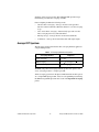
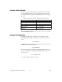
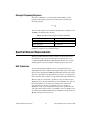
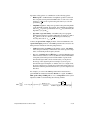
USER GUIDE
NI Spectral Measurements Toolkit
This document explains how to use the NI Spectral Measurements Toolkit
(SMT) in LabVIEW and LabWindows™/CVI™ for frequency-domain
measurements.
Contents
Conventions ............................................................................................ 2
Using the Spectral Measurements Toolkit .............................................. 3
Integrating the Spectral Measurements Toolkit............................... 4
Locating the Spectral Measurements Toolkit .................................. 4
SMT Programming Flow Diagram ......................................................... 5
Advanced-Level VIs ........................................................................ 6
Using LabVIEW Spectral Measurements Examples .............................. 7
SMT Simulation Examples .............................................................. 7
SMT Spectrum Analyzer (simulated)....................................... 7
SMT ACP (simulated) .............................................................. 8
Using LabWindows/CVI Spectral Measurements Examples ................. 9
Continuous Zoom FFT..................................................................... 9
Frequency Response Measurement ................................................. 9
Cross Power Spectrum Measurement .............................................. 10
Using Spectral Measurements Toolkit Techniques ................................ 10
Zoom FFT ........................................................................................ 10
Continuous Zoom FFT..................................................................... 12
Block Zoom FFT ............................................................................. 14
Determining When to Use Continuous or Block Zoom FFT........... 14
Zoom Spectrogram .......................................................................... 15
Configuring Zoom FFT VIs.................................................................... 18
Center Frequency and Span ............................................................. 18
Resolution Bandwidth, Spectral Lines, and Window ...................... 20
Choosing Useful Configuration Parameters .................................... 22
Spectral Domain Averaging.................................................................... 24
Averaging Conventions ................................................................... 25
Averaging Options ........................................................................... 26
Averaged FFT Spectrum.................................................................. 27
Averaged Power Spectrum .............................................................. 28
Averaged Cross Spectrum ................................................................28
Averaged Frequency Response ........................................................29
Spectral Domain Measurements ..............................................................29
Unit Conversion................................................................................29
Peak Search and Amplitude/Frequency Estimation .........................31
Power in Band ..................................................................................32
Adjacent Channel Power (ACP).......................................................32
Occupied Bandwidth (OBW) ...........................................................33
Where to Go for Support .........................................................................34
Conventions
The following conventions are used in this manual:
»
The » symbol leads you through nested menu items and dialog box options
to a final action. The sequence File»Page Setup»Options directs you to
pull down the File menu, select the Page Setup item, and select Options
from the last dialog box.
<>
Italic text enclosed in angle brackets represents directory names and
parts of paths that may vary on different computers, such as
<Windows\System>.
This icon denotes a note, which alerts you to important information.
bold
Bold text denotes items that you must select or click in the software, such
as menu items and dialog box options. Bold text also denotes parameter
names and palette names.
italic
Italic text denotes variables, emphasis, a cross-reference, or an introduction
to a key concept. Italic text also denotes text that is a placeholder for a word
or value that you must supply.
monospace
Text in this font denotes text or characters that you should enter from the
keyboard, sections of code, programming examples, and syntax examples.
This font is also used for the proper names of disk drives, paths, directories,
programs, subprograms, subroutines, device names, functions, operations,
variables, filenames, and extensions.
monospace italic
Italic text in this font denotes text that is a placeholder for a word or value
that you must supply.
NI Spectral Measurements Toolkit User Guide
2
ni.com
Using the Spectral Measurements Toolkit
The Spectral Measurements Toolkit contains LabVIEW VIs and
LabWindows/CVI functions that perform the following operations:
•
Zoom frequency analysis—Zoom fast Fourier transform (FFT)
functions and VIs allow you to zoom in on a narrow frequency range
in a spectrum.
•
Spectrum averaging—The Spectral Measurements Toolkit supports
averaging types such as root-mean-square (RMS) averaging, vector
averaging, and peak-hold averaging.
•
Spectral measurements—The Spectral Measurements Toolkit contains
functions and VIs that can measure power-in-band and adjacent
channel power.
•
Unit conversion—The Spectral Measurements Toolkit unit conversion
supports typical radio frequency (RF) units, such as volts RMS
squared (V2rms), decibel (dB), decibel milliwatts (dBm), and dBm per
hertz (dBm/Hz). You can use the Spectral Measurements Toolkit to
convert a raw FFT spectrum to a power spectrum or power spectral
density for noise measurements.
•
Peak power and frequency determinations—The Spectral
Measurements Toolkit includes a spectrum peak search algorithm
that determines peak levels and frequency.
•
Zoom processing configuration—The Spectral Measurements Toolkit
configuration functions and VIs allow you to use conventional
measurement settings, such as center frequency, span, and resolution
bandwidth (RBW) to configure zoom processing. The configuration
functions and VIs return an acquisition size based on your spectrum
settings.
•
Spectrogram—The Spectral Measurements Toolkit contains VIs that
allow you to compute joint-time and frequency-domain calculations
and display the results as a spectrogram. This feature is supported only
in LabVIEW.
•
Analog modulation—The Spectral Measurements Toolkit supports
analog modulation to perform amplitude, frequency, and phase
modulation and demodulation. Functions and VIs are included to
perform upconversion and downconversion on baseband and passband
signals.
© National Instruments Corporation
3
NI Spectral Measurements Toolkit User Guide
Integrating the Spectral Measurements Toolkit
You can use the Spectral Measurements Toolkit for the following
applications:
•
•
•
Frequency-domain measurements such as:
–
Adjacent channel power ratio (ACPR)
–
Channel spectrum
–
Power-in-band measurements
–
Average and peak power
–
Power spectral density
–
Spectrum limit and mask testing
Modulation-domain measurements such as:
–
Frequency deviation
–
AM modulation index
Component-level measurements such as characterization of
oscillators, mixers, and filters
Locating the Spectral Measurements Toolkit
The Spectral Measurements Toolkit contains LabVIEW VIs and
LabWindows/CVI functions. In LabVIEW, Spectral Measurements
Toolkit VIs are located on the Functions»RF Communications»
Spectral Measurements and Functions»Addons»Modulation palettes.
SMT functions are located on the LabWindows/CVI function panel
under Library»Spectral Measurements Toolset and Library»
Analog Modulation.
Some Spectral Measurements Toolkit VIs and functions configure hardware,
meaning their operation requires installing specific hardware instrument drivers. For
more information about supported hardware, refer to the NI Spectral Measurements
Toolkit Readme, located at Start»All Programs»National Instruments»
Spectral Measurements.
Note
For simplicity, this document pertains only to using VIs in the LabVIEW
development environment, except in the Using LabWindows/CVI Spectral
Measurements Examples section. In most cases, the same guidelines apply
to using functions in the C programming environment.
Note Documentation for LabWindows/CVI functions can be found in the NI Spectral
Measurements Function Reference Help, located at Start»All Programs»National
Instruments»Spectral Measurements»CVI Support.
NI Spectral Measurements Toolkit User Guide
4
ni.com
SMT Programming Flow Diagram
Programming flow diagrams are flowcharts that depict the most effective
order for programming Spectral Measurements Toolkit VIs. Use the
programming flow diagram in the SMT Programming Flow VI as a visual
guide for the order in which you should call VIs. This VI is located in
the <LabVIEW >\examples\Spectral Measurements Toolset\
Simulation folder. The example is not intended to be executable,
but rather to supply an informative block diagram depicting general
programming for applications using acquired or simulated data. Figure 1
shows the LabVIEW programming flow diagram for these applications.
Figure 1. SMT Programming Flow Diagram
The following steps describe the general programming flow of the Spectral
Measurements Toolkit.
1.
© National Instruments Corporation
Enter the time-domain data into the SMT Basic Zoom Power
Spectrum VI. This VI specifies the zoom settings in terms of only
center frequency and span. The VI performs zoom FFT processing and
returns a power spectrum in units V2rms.
5
NI Spectral Measurements Toolkit User Guide
2.
3.
Enter the output power spectrum into an SMT measurement VI
and/or use the SMT Spectrum Unit Conversion VI as follows:
a.
Enter the output power spectrum into an SMT measurement VI:
the SMT Power in Band, the SMT Adjacent Channel Power, or the
SMT Occupied Bandwidth VI. These VIs accept a power
spectrum with units V2rms and return the requested measurements.
Perform the measurements on only an unscaled power spectrum.
You can specify the units in which to view these measurements.
b.
Use the SMT Spectrum Unit Conversion VI to display the power
spectrum in units other than the default, V2rms. The VI allows you
to convert the raw data into the following units: watts, volts, or
variations of dB such as dBm, dBW, and dBV. You can specify
different scaling factors such as RMS or peak.
Use the SMT Spectrum Peak Search VI to find specific tones or
peaks in the spectrum. The SMT Spectrum Peak Search VI accepts
only a unit-converted power spectrum. You must specify the threshold
level in the same units as the power spectrum. The VI detects any peak
above the threshold level as a valid peak.
Advanced-Level VIs
The zoom processing capability of the SMT Basic Zoom Power
Spectrum VI is limited by the size of the data previously acquired. Use
the VIs located on the SMT Advanced palette to control zoom settings or
additional settings such as window type, RBW, number of spectral lines,
and RBW definition.
Complete the following steps when using the advanced-level VIs of the
programming flow diagram in the SMT Programming Flow VI:
1.
Use the SMT Config Zoom FFT VI to configure the zoom settings. Use
the default values for the spectrum settings control if you are unsure
of the settings. The VI uses the values you enter to recommend an
acquisition size or a data size. The VI also maps measurement-specific
settings to classical analysis settings.
2.
Enter a time-domain signal of the size recommended by the SMT
Config Zoom FFT VI into the SMT Zoom Power Spectrum VI.
You must pass the SMT zoom settings parameter from the SMT
Config Zoom FFT VI to subsequent VIs to ensure accurate data. The
SMT Zoom Power Spectrum VI performs zoom FFT processing and
returns a power spectrum with units V2rms.
3.
Enter the output power spectrum into subsequent measurement VIs
using the guidelines in steps 2 and 3 of the SMT Programming Flow
Diagram section.
NI Spectral Measurements Toolkit User Guide
6
ni.com
For an averaged power spectrum with zoom, use the SMT Zoom Power
Spectrum VI. For an averaged FFT spectrum, which has a complex
output for magnitude and phase calculations, use the SMT Zoom FFT VI
first and then the SMT Averaged FFT Spectrum VI. If you have two
channels of input time-domain data and want cross power spectrum or
frequency-response measurements, use the SMT Zoom FFT Spectrum VI
first and then the SMT Averaged Cross Spectrum VI or the SMT Averaged
Frequency Response VI.
Using LabVIEW Spectral Measurements Examples
This section describes some of the examples located in the <LabVIEW >\
examples\Spectral Measurements Toolset folder. If you are
programming in C, refer to the Using LabWindows/CVI Spectral
Measurements Examples section.
SMT Simulation Examples
The Simulation folder contains examples that are hardware-independent
and use a simulated signal generated by the host computer. All examples
contain the word “simulated” in their names.
SMT Spectrum Analyzer (simulated)
The SMT Spectrum Analyzer (simulated) VI demonstrates how to
use SMT VIs to build a spectrum analyzer with zoom and averaging
capabilities. This VI is located in the Simulation folder inside the
Spectral Measurements Toolset folder.
The SMT Config Zoom FFT VI specifies the zoom settings, returning
the SMT zoom settings cluster. This cluster is wired to the SMT zoom
settings parameter of the SMT Zoom Power Spectrum VI. The spectral
info cluster that the SMT Zoom Power Spectrum VI returns is wired to the
spectral info parameter on the SMT Spectrum Unit Conversion VI.
In this example, the spectrum settings parameter specifies the zoom
settings in terms of center frequency, span, and RBW. The example uses the
default value for the resolution bandwidth, –1.00, which implies that the
software calculates the RBW value based on other inputs to the
configuration VIs. The SMT Config Zoom FFT VI, located on the SMT
Advanced palette, uses these settings to recommend an acquisition size.
This VI also returns the actual spectrum settings, which appear directly
below the spectrum graph. In the example, the SMT Config Zoom FFT VI
calculates span as 4.96 MHz and the resolution bandwidth as 30.88 kHz.
© National Instruments Corporation
7
NI Spectral Measurements Toolkit User Guide
The averaging parameters cluster specifies the following settings:
•
Averaging type, such as vector averaging, RMS averaging,
or peak hold
•
Weighting type, such as linear or exponential
•
Averaging size
The linear weighting mode parameter specifies a type of linear weighting.
The SMT Zoom Power Spectrum VI, located on the SMT Advanced
palette, returns the spectrum in units of V2rms.
The unit conversion settings parameter specifies the units in which to
display the spectrum. For example, you can set units to dBm, peak scaling
to RMS, and psd? to on to view the power spectrum as power spectral
density (PSD).
The spectrum parameter is a waveform graph that shows the spectrum of
the simulated signal, which is a 12.00 MHz sine wave with added white
noise. The center of the spectrum appears at 12.00 MHz, the center
frequency, and the spectrum spans from 9.523 MHz to 14.483 MHz.
Use the peak search settings parameter to find the peaks in the example
spectrum. In the parameter, specify whether to find Single Max Peak or
Multiple Peaks, and enter the threshold level value above which a peak is
valid. The peak threshold level uses the same unit of measurement as the
spectrum.
The number of peaks parameter shows the number of peaks that meet the
threshold criteria, and the peaks parameter shows the frequency and Y-axis
values for these peaks.
SMT ACP (simulated)
The SMT ACP (simulated) VI demonstrates how to use SMT VIs
to perform measurements on a spectrum. This VI is located in the
Simulation folder. The example shows one specific measurement, the
adjacent channel power (ACP). You can also perform other measurements,
such as power in band and occupied bandwidth (OBW).
The example uses the SMT Config Zoom FFT VI to configure the zoom
FFT. The SMT zoom settings parameter from the SMT Config Zoom FFT
VI is wired to the SMT zoom settings parameter of the SMT Zoom Power
Spectrum VI. The example performs the ACP measurement on the raw
power spectrum before the unit conversion.
Perform the adjacent channel power measurement on an unscaled power spectrum
before calling the SMT Spectrum Unit Conversion VI.
Note
NI Spectral Measurements Toolkit User Guide
8
ni.com
The channel specification parameter specifies the center frequency,
bandwidth, and spacing for the ACP measurement. The bandwidth
parameter specifies the width of each channel. The spacing parameter
specifies the separation between the center frequencies of each channel.
The Units [rms] parameter specifies the units for the ACP measurement.
The Power Spectrum parameter is a waveform graph that shows the power
spectrum with the three channels, or bands, and the power in each channel.
The Advanced Settings tab of the example includes some of the same
controls as the SMT Spectrum Analyzer (simulated) example, such as
Averaging Parameters.
Using LabWindows/CVI Spectral Measurements
Examples
This section describes some of the LabWindows/CVI programming
examples located in the <LabWindows/CVI>\samples\smt folder. You
can use these example programs as a starting point for your applications.
The simulated folder contains examples that use a simulated source. Use
these examples to explore different features of the Spectral Measurements
Toolkit without using a data acquisition device.
Continuous Zoom FFT
The Continuous Zoom FFT example is located at samples\smt\
simulated\smtcz\smtcz.prj.
This example demonstrates how to configure the zoom FFT, then calculates
an averaged power spectrum using the continuous zoom FFT technique.
It demonstrates how to display the spectrum in different RF units.
Frequency Response Measurement
The Frequency Response Measurement example is located at samples\
smt\simulated\smtfqres\smtfqres.prj.
This example demonstrates how to configure the zoom FFT, then calculates
the averaged frequency response of a stimulus and response signal from
a device under test. The example uses the block zoom FFT technique.
The example uses handles to maintain state information between functions,
such as SmtConfigZoomFFT and SmtZoomFFT.
© National Instruments Corporation
9
NI Spectral Measurements Toolkit User Guide
Cross Power Spectrum Measurement
The Cross Power Spectrum Measurement example is located at samples\
smt\simulated\smtcrspwr\smtcrspwr.prj.
This example demonstrates how to configure the zoom FFT, then calculates
the averaged power spectrum of a stimulus and response signal from
a device under test and the averaged cross spectrum between these
two signals. The example uses the continuous zoom FFT technique and
demonstrates how you must create a unique handle for the stimulus data
(handle1) and response data (handle2). Use handle1 when you calculate
the continuous zoom FFT and averaged power spectrum on the stimulus.
Use handle2 when you calculate the continuous zoom FFT and averaged
power spectrum on the response. You can use either handle1 or handle2
when you calculate the averaged cross power spectrum between the
stimulus and the response.
Using Spectral Measurements Toolkit Techniques
The Spectral Measurements Toolkit contains tools for block and
continuous zoom processing and spectrum averaging. You can specify the
zoom characteristics in terms of center frequency, span, and resolution
bandwidth. You can use spectrum averaging to reduce the effect of noise
on your measurement system.
Zoom FFT
The Spectral Measurements Toolkit uses the zoom FFT technique to
analyze the frequency spectra of stationary signals. This technique allows
you to zoom in on a small portion of the frequency spectrum with
high-frequency resolution by using fewer calculations than a standard FFT.
Figure 2 illustrates how a zoom FFT detects the presence of two tones of
closely spaced frequencies. The standard FFT, shown in the upper graph,
indicates a single peak, and the zoom FFT, shown in the lower graph,
indicates the presence of two separate tones in the signal.
NI Spectral Measurements Toolkit User Guide
10
ni.com
Figure 2. Zoom FFT Technique
FFT algorithms usually perform baseband analysis by displaying the
spectrum from zero to the Nyquist frequency. However, a standard FFT
might not be effective if you need to obtain a higher frequency resolution
over a limited portion of the spectrum or if you need to zoom in on details
of a spectral region. The zoom FFT uses algorithms to avoid the amount of
calculation required using a long standard FFT to obtain high-frequency
resolution over an entire spectrum.
You can define the frequency resolution of an analysis, df, using the
following formula:
df = fs /N = 1/T
where
fs is the frequency of the sampled signal
T is the time duration
N is the number of samples
Only the acquisition time determines the analysis resolution. You can either
decrease fs or increase N to improve df.
The Spectral Measurements Toolkit supports two algorithms for zoom FFT
processing: continuous zoom FFT and block zoom FFT.
© National Instruments Corporation
11
NI Spectral Measurements Toolkit User Guide
Continuous Zoom FFT
Continuous zoom FFT is a technique for quickly analyzing data as it
arrives. A decimation process reduces the sample rate in real time. After the
process acquires all the data and decimates it in time T, a relatively small
FFT remains. The term continuous refers to beginning the process while
data arrives. With a standard FFT, you must wait until all the data arrives
before beginning calculations.
The continuous zoom FFT first shifts the spectral region of interest into
the baseband. The technique then applies a lowpass antialias filter and
decimates, or downsamples, the data by a factor of M. The zoom factor of
M yields a new effective sample rate, fs /M. The antialias filter has a cutoff
frequency of fs /(2 × M) because the Nyquist frequency has decreased by
a factor of M.
After lowpass filtering, the continuous zoom FFT performs an FFT on the
reduced sample rate data to produce the zoom spectrum. This technique is
destructive because the original data changes as a result of the filtering and
decimation. If you store the data and batch process it later, you lose the
primary benefit of the technique, which is its real-time capability. Figure 3
shows the basic steps of frequency shifting, decimation, and FFT.
Modulation
x(n)
fs
Lowpass Filter
Decimate by M
fs/M
Fixed Size
FFT
Zoom Processor
Figure 3. Continuous Zoom FFT Diagram
Although it might seem possible to reduce the sample rate, fs, to improve
frequency resolution, this method does not work. You cannot acquire the
data with a lower sample rate to increase resolution because the Nyquist
sampling theorem applies. In the original acquisition, you must sample at
least twice as fast as the highest frequency of your desired zoom region to
obtain the frequency information you need. You cannot reduce the sample
rate until after frequency shifting occurs if you want to improve the
frequency resolution of the zoom region. The continuous zoom FFT shifts a
high-frequency signal into the baseband before adjusting the sample rate.
NI Spectral Measurements Toolkit User Guide
12
ni.com
The continuous zoom FFT technique is sometimes called the real-time
zoom FFT because it continuously performs the frequency shifting,
decimation, and filtering processes on the arriving data. The FFT operation
itself cannot proceed until you acquire all the data. The FFT operation then
occurs in parallel with the next data acquisition.
You can use the SMT Cont Zoom FFT VI to perform the continuous zoom
FFT technique. This VI is located on the Zoom FFT palette, which is a
subpalette of the SMT Advanced palette. This VI also passes the complex
modulated and filtered time-domain data corresponding to the spectrum.
Figure 4 shows the in-phase (I) and quadrature-phase (Q) components
of this complex time-domain data plotted on an I versus Q plot. The input
signal is a phase-modulation (PM) wave. The PM signal is modulated with
a square wave, with a carrier at 70 MHz. The RF signal analyzer is tuned to
the carrier frequency.
15.0m
14.0m
12.0m
10.0m
8.0m
6.0m
Q (Volts)
4.0m
2.0m
0.0
–2.0m
–4.0m
–6.0m
–8.0m
–10.0m
–12.0m
–14.0m
–15.0m
–15.0m
–10.0m
–5.0m
1.7a
I (Volts)
5.0m
10.0m
15.0m
Figure 4. I/Q Plot
© National Instruments Corporation
13
NI Spectral Measurements Toolkit User Guide
Block Zoom FFT
Use a block zoom FFT in situations when you cannot access data until the
data acquisition is complete. The block zoom FFT is a nondestructive zoom
FFT because it stores data before processing, so the data is available in its
original form if you need it for other operations. The block zoom FFT is an
algorithm that calculates a portion of a large FFT. The block zoom FFT also
improves the frequency resolution, df, by increasing the number of points
that the FFT processes.
A block zoom FFT uses only the part of a large FFT that represents the
frequency range you analyze. For example, if the input data has a length
L × M, an FFT on the original data results in L × M points of FFT spectrum.
To analyze only 1/M of the whole spectrum, or L frequency bins, use a
block zoom FFT. The block zoom FFT computes L points of the original
L × M point spectrum faster and with fewer calculations than if you
perform a large FFT on the entire data set and remove the unwanted
portion.
Perform the block zoom FFT technique by using the SMT Zoom FFT VI.
This VI is located on the Zoom FFT palette, which is a subpalette of the
SMT Advanced palette.
Determining When to Use Continuous or Block Zoom FFT
Choosing which zoom FFT to use for a particular application depends
on many factors, including system speed, memory, acquisition rate, and
application requirements.
An advantage of the continuous zoom FFT is that you can update the results
continuously to give a smooth display and minimize the time it takes for
transients to appear in the displayed spectrum. You can control the update
time with the %overlap parameter of the advanced settings cluster of the
SMT Config Cont Zoom FFT VI. This VI is located on the SMT Advanced
palette. A setting of 0% updates like a block zoom FFT and waits for the VI
to process an entire new data set before returning a result. A setting of 50%
updates twice as fast as a setting of 0% by reusing the last half of the
previous data block to return an updated result after the VI acquires and
processes half of the new data set.
You cannot predict whether the continuous zoom FFT can sustain a certain
acquisition rate in real time, so the best option is to try running the
application using the SMT Cont Zoom FFT VI. If you receive buffer
overflow errors from the acquisition VI, either reduce the acquisition
rate or use the block zoom technique.
NI Spectral Measurements Toolkit User Guide
14
ni.com
The block zoom FFT is a general-purpose technique that works best as a
post-processing method. The block zoom FFT also is useful for real-time
applications where the data rate is too high for a continuous zoom FFT to
sustain in real time. To process the entire data set, provide enough memory
to store the data until the FFT can process it. If processing every data point
is not critical, use the block zoom FFT with the latest data available.
Zoom Spectrogram
A spectrogram is the result of joint time-frequency analysis (JTFA)
processing. The Spectral Measurements Toolkit implements the short-time
Fourier transform (STFT) with a zoom FFT to give a zoom spectrogram.
The SMT Zoom STFT VI calculates FFTs on equivalent segments of your
signal at fixed time intervals. This VI applies a window to each signal
segment, calculates an FFT on the windowed segment, and arranges the
resulting FFTs in chronological order. Figure 5 illustrates the process.
Note STFT VIs are located in the <LabVIEW >\vi.lib\addons\Spectral
Measurements Toolset folder.
© National Instruments Corporation
15
NI Spectral Measurements Toolkit User Guide
Time Span
1.0
0.8
Amplitude
0.6
Window
0.4
0.2
Signal
0.0
–0.2
–0.4
–0.6
10
0
30
20
40
Time (µs)
50
60
70
75
FFT
FFT
F
T
Figure 5. Spectrogram Process Example
The SMT Config Zoom STFT VI specifies the spectrogram in terms of
its center frequency, frequency span, and time span. The frequency span
controls the FFT zoom. If the center frequency is 10 MHz and the span is
2 MHz, the SMT Config Zoom STFT VI calculates the spectrogram from
9 MHz to 11 MHz. The time span specifies the time interval from the center
of the first window to the center of the last window. The VI also has
advanced parameters for specifying the spectrogram, including window,
resolution bandwidth, RBW definition, frequency points, time points, and
NI Spectral Measurements Toolkit User Guide
16
ni.com
effective band specification. If you leave the default advanced parameters,
the configuration VI calculates the correct parameters for a spectrogram
with evenly distributed time and frequency resolution on a square display
area. If the display area is not square, enter an aspect ratio for the display
area in the aspect ratio parameter. Figure 6 shows an example of a
completed spectrogram with a center frequency of 16 MHz and a span
of 16 MHz.
18 µ
s
15 µ
s
12 µ
s
z
6 µs
z
MH
3 µs
Hz
0 µs
0M
8M
Hz
MH
16
24
32
MH
z
9 µs
Figure 6. Spectrogram Example
© National Instruments Corporation
17
NI Spectral Measurements Toolkit User Guide
Configuring Zoom FFT VIs
When using Spectral Measurements Toolkit VIs, you must enter several
values to completely specify a zoom FFT. The Spectral Measurements
Toolkit provides two configuration VIs that select values for each setting
and that require you to enter a minimal number of values. The SMT Config
Zoom FFT VI configures the block zoom FFT. The SMT Config Cont
Zoom FFT VI configures the continuous zoom FFT. These configuration
VIs ensure that the input values are compatible and yield valid results.
Enter values for specific settings, and the configuration VIs calculate
the rest.
Center Frequency and Span
The two fundamental characteristics of a zoom FFT are center frequency,
which is the location of the zoom within the spectrum, and span, which
is the degree to which the FFT zooms in. For basic zoom applications,
center frequency and span are often the only values you must enter.
The following restrictions apply to the input values for center frequency
and span:
•
center frequency must fall within the effective band of the input
signal. The effective band is the frequency band in which the data from
the input signal is valid. You can use the effective band to exclude the
roll-off region of an analog antialiasing filter from consideration.
The effective band defaults to the full bandwidth of the input signal,
up to half the sample rate. If the specified frequency falls outside the
effective band, the configuration VI uses the center of the effective
band as the center frequency.
•
span must be smaller than the effective band because you can only
zoom in on the spectrum. You cannot zoom out. If span is larger than
the effective band, the configuration VI sets the span to the largest
value that does not fall outside of the effective band.
•
When you combine center frequency and span, neither endpoint of
the desired frequency span can fall outside the frequency range of the
effective band. If both center frequency and span meet the previously
stated restrictions, but a portion of the zoom span region falls outside
the effective band, the configuration VI moves the center frequency far
enough to ensure that the entire span is inside the effective band.
NI Spectral Measurements Toolkit User Guide
18
ni.com
The left side of Figure 7 shows examples of the four combinations of
center frequency and span that you can encounter in the case of a real
input signal. The right side of Figure 7 shows the actual coerced values of
center frequency and span that the VI sets in each example.
Antialiasing Filter Response
a.
User Input
Coerced Result
Effective Band
Effective Band
Span
Span
fh
fc
fl
fs/2
Effective Band
b.
fc
fl
fh
fl
fc
fc = (fl + fh)
2
fl
fs/2
fs/2
fh
fs/2
fh
fs/2
Effective Band
Span
Span
fc
fh
fl
fs/2
Effective Band
d.
fh
Span
Effective Band
fl
fs/2
Effective Band
Span
c.
fh
fc
Effective Band
Span
Span
fl fc
fh
fl
fs/2
fc +
Figure 7. Center Frequency and Span Combinations
Figure 7a demonstrates that if you enter appropriate values for both center
frequency and span, the values do not change. The spectrum represents the
frequency response of the input antialiasing filter on the data acquisition
device. Figure 7b demonstrates that if you enter a center frequency value
© National Instruments Corporation
19
NI Spectral Measurements Toolkit User Guide
that is outside the effective band, the span changes to the default value,
which is the center of the effective band. Figure 7c demonstrates that if
you request a span that is wider than the effective band, the span decreases
until it falls entirely within the effective band without moving the center
frequency. Figure 7d demonstrates that if you enter center frequency and
span values that fall within acceptable limits but a portion of the span falls
outside the effective band, the center frequency moves until the span falls
entirely within the effective band.
Resolution Bandwidth, Spectral Lines, and Window
The FFT process is equivalent to passing the time-domain signal through
a bank of bandpass filters with center frequencies that correspond to
frequencies of the FFT bins. The shape of the equivalent filter is determined
by the window applied to the time-domain signal. The resolution
bandwidth control represents the width of an equivalent filter corresponding
to a single FFT bin. You can specify this width in one of several ways
through the RBW definition parameter in the SMT configuration VIs. The
options are 3 dB, 6 dB, ENBW, and bin width. Both 3 dB and 6 dB define
the resolution bandwidth in terms of the distance between the two points
at which the filter response fell by the specified amount as compared to
the peak response, as shown in Figure 8. Effective noise bandwidth (ENBW)
defines the resolution bandwidth as the bandwidth of an ideal rectangular
response filter, which has the same power output as the equivalent bandpass
filter for a given white noise input. Bin width defines the resolution
bandwidth as the distance from the center of one frequency bin to the
next—independent of the equivalent filter shape. The default value of RBW
definition is 3 dB.
Figure 8. Main and Side Lobes of a 7-Term Blackman-Harris Window
NI Spectral Measurements Toolkit User Guide
20
ni.com
Figure 8 shows the shape of the equivalent filter corresponding to a 7-Term
Blackman-Harris window. The cursors are placed at the 3 dB points of the
filter response, and the resolution bandwidth is the distance between the
cursors.
spectral lines controls how many frequency bins are present in the zoom
spectrum result that the VI displays. If you request more spectral lines
than resolution bandwidth requires, the parameter zero-pads the FFT to
interpolate the spectrum to the desired number of lines.
window controls the window applied to the time-domain signal. The
major benefit of windowing is to confine spectral leakage to the main lobe,
thereby reducing it in the side lobes, as shown in Figure 8. The window
determines the shape of the equivalent filter of an FFT bin; therefore,
the window choice influences any calculations involving the resolution
bandwidth.
The configuration VIs use resolution bandwidth, spectral lines, and
window to determine the acquisition size, which is the number of points
that you must acquire for a particular zoom operation. You must specify
a value in at least one of the two parameters: resolution bandwidth or
spectral lines. If you specify a value in only one parameter, the value
determines the acquisition size, and the acquisition size value determines
the value of the other parameter. If you specify both resolution bandwidth
and spectral lines, the VI compares the acquisition size that each parameter
requires and uses the smaller of the two as the actual acquisition size. For a
real input signal, the acquisition size that the spectral lines value determines
is calculated by the following formula:
acquisition size = 2 × spectral lines × zoom factor
where zoom factor relates the zoom span to the full spectrum as follows:
fs ⁄ 2
zoom factor = ---------span
For a real input signal, the acquisition size that the resolution bandwidth
value determines is calculated by the following formula:
[ 3 dB BW ] × f
acquisition size = ------------------------------------s
RBW
© National Instruments Corporation
21
NI Spectral Measurements Toolkit User Guide
The acquisition size comes from the following basic relationship:
df = fs /N = 1/T
where N is equal acquisition size and RBW is the frequency resolution df
multiplied by the window spectral leakage correction factor of 3 dB
bandwidth.
If the spectral lines value requires a larger acquisition size than the
resolution bandwidth value requires, the VI uses zero-padding to
determine the number of FFT lines you need. If the resolution bandwidth
value requires a larger acquisition size than the spectral lines value
requires, the VI coerces resolution bandwidth to a value consistent with
the acquisition size you need and returns the value as actual resolution
bandwidth.
You might see actual values differ slightly from the values you need in two cases.
If the span and sampling frequency you need correspond to a zoom factor that is not an
integer, the VI coerces the zoom factor to an integer value, and the span varies accordingly.
The acquisition size also might vary slightly to ensure that you can use an efficient FFT
algorithm to optimize performance.
Note
Choosing Useful Configuration Parameters
The choice of center frequency, span, and window type is application
dependent. For example, when testing CDMA signals, you might specify
a center frequency of 834 MHz and a span of 2 MHz. SMT supports nine
window types. 7-Term Blackman-Harris, which is the default window
type, has the highest dynamic range and is ideal for signal-to-noise ratio
type applications. The choice of spectral lines depends on the display
resolution you require on the plot.
The choice of RBW depends on a number of factors, such as the spacing
between the two tones that you want to identify and the amplitude of
these tones.
NI Spectral Measurements Toolkit User Guide
22
ni.com
Figure 9 shows the spectrum of a multitone signal calculated using
two RBW values. The multitone signal consists of two tones, at frequencies
1.0 MHz and 1.1 MHz, separated by 100 kHz. Table 1 shows the trade-offs
of using two different RBWs.
Table 1. Larger versus Smaller RBW
Larger RBW (103.5 kHz)
Smaller RBW (9.94 kHz)
Smaller FFT size, requiring less computation
time
Larger FFT size, requiring more computation
time
Cannot distinguish between the two tones in
the spectrum
Can distinguish between the two tones in
the spectrum
An RBW of 103.5 kHz is not sufficient to distinguish between two tones that
are 100 kHz apart.
Note
Figure 9. RBW Example
© National Instruments Corporation
23
NI Spectral Measurements Toolkit User Guide
Spectral Domain Averaging
Averaging is an important part of spectrum-domain measurements because
of the effects of noise on a signal and its spectrum. The Spectral
Measurements Toolkit includes averaging VIs that average several
records of data to reduce the noise effects. You can use the three different
averaging types: vector, RMS, and peak-hold.
Vector averaging lowers the noise floor while retaining the signal
spectrum. In the time domain, a running average reduces the effect of
zero-mean white noise on a signal. The noise is averaged out while the
signal is retained. The signal must be triggered, meaning that each data
record starts at a consistent point in the periodic signal, preserving the
signal integrity during an averaging process. Because the FFT is a linear
transform, averaging spectral records in the frequency domain is equivalent
to averaging data records in the time domain. The signal must be triggered
for vector averaging to work properly. Vector averaging requires a complex
spectrum and produces a complex result that you can convert to a real
power spectrum.
If the signal is not triggered in the time domain, phase noise appears in the
resulting spectrum. You can use RMS averaging to eliminate the effect of
phase noise. The magnitude of the spectrum is independent of time shifts
of the input signal, but the phase can change dramatically with each data
record. If you average the power spectra and take the square root of the
result, you eliminate the effect of phase variations. You can no longer
reduce the noise floor, but you can reduce the magnitude variance of the
noise. Reducing the noise variance helps to distinguish small frequency
peaks from the largest noise peaks. RMS averaging eliminates all phase
information and returns a real spectrum. If the averaging process
returns results in a complex data type, the imaginary portion is zero.
Peak-hold averaging refers to a method of retaining the maximum
magnitude value of every frequency bin over several data records.
Peak-hold averaging is most useful for capturing transient phenomena
that do not appear in individual spectra. In a monitoring application, the
peak-hold display allows an operator to tell at a glance if a transient at
a certain frequency occurred since the last reset. However, peak-hold
averaging cannot specify when the transient happened. Like RMS
averaging, peak-hold averaging results in a real spectrum.
When you apply a zoom FFT VI to a signal, you receive the complex
FFT spectrum. The spectrum domain averaging functions can operate on
the FFT spectrum to return different types of spectra, such as averaged
FFT spectrum, power spectrum, cross spectrum, and frequency response.
NI Spectral Measurements Toolkit User Guide
24
ni.com
The averaging VIs require that you enter an FFT spectrum as a complex
array. You can perform spectrum unit conversion before or after averaging.
Averaging Conventions
For Spectral Measurements Toolkit VIs, averaging refers to the average of
several different data sets from the same process. The following list
contains averaging operations that apply independently to each frequency
bin of the Fourier transform.
FR + jFI
The complex representation of the Fourier transform
of a signal f(t) using real and imaginary values.
< F >k = FR + jFI
For vector averaging, real and imaginary parts of the
Fourier transform are averaged separately using either
linear or exponential weighting over k data records.
|F|
The magnitude of the Fourier transform.
Xk, Yk
kth instance of input spectrum X and its averaged
output Y.
max(Xk, Yk)
Each complex frequency of spectrum Xk is compared
in magnitude to its counterpart in Yk. The larger value
is retained. The result is a real spectrum.
conj( )
Complex conjugate.
© National Instruments Corporation
25
NI Spectral Measurements Toolkit User Guide
Averaging Options
Figure 10 illustrates the options available for spectrum averaging.
Averaging
Type
No Averaging
Peak-Hold
Weighting
Type
Linear
Weighting
Mode
RMS
Exponential
Linear
One Shot
Auto Restart
Vector
Moving Average
Continuous
Average Size
Figure 10. Spectrum Averaging Options
The averaging processes apply weighting to the < > operator in both RMS
and vector averaging as shown in the following equation:
Yk = <X>k = a1 × Yk – 1 + a2 × Xk
where Yk is the new average, Yk – 1 is the previous average, and Xk is the new
measurement.
For linear weighting,
a1 = (k – 1)/k, and a2 = 1/k
For exponential weighting,
a1 = (k – 1)/k and a2 = 1/N for k ≤ N,
a1 = (N – 1)/N and a2 = 1/N for k > N
where N is a user-specified constant that determines how much weight
is given to recent data relative to older data. Small values of N place more
NI Spectral Measurements Toolkit User Guide
26
ni.com
emphasis on the most recent data. The averages sofar parameter stops
incrementing at N while the averaging continues.
Linear weighting includes the following modes:
•
One-shot linear averaging—Average one time for the specified
duration of N measurements. When the duration is over, the averaging
stops.
•
Auto–restart linear averaging—Automatically repeat the one-shot
linear averaging after every N measurements.
•
Moving average—Average the most recent N measurements.
•
Continuous—Average all measurements taken with equal weight.
Averaged FFT Spectrum
The following equations describe the three averaging methods applied to a
complex FFT spectrum.
Table 2. FFT Averaging Methods and Equations
Averaging Method
Equation
Vector averaging
Yk = <X>k
RMS averaging
Yk =
Peak-hold averaging
Yk = max(Xk, Yk – 1)
( <X conj ( X )> k )
The RMS and peak-hold averaging methods produce real spectra, and
vector averaging produces a complex spectrum.
All the averaging operations in the Spectral Measurements Toolkit operate
on a complex FFT input spectrum. Create an averaged FFT spectrum using
the SMT Averaged FFT Spectrum VI, located on the Spectrum Averaging
palette.
© National Instruments Corporation
27
NI Spectral Measurements Toolkit User Guide
Averaged Power Spectrum
The following equations describe the averaging methods you can apply
to a complex FFT spectrum to yield an averaged power spectrum. The
No averaging method converts the complex FFT spectrum to a real power
spectrum.
Table 3. Averaged Power Spectrum Averaging Methods and Equations
Averaging Method
Equation
No averaging
Y = X conj(X)
Vector averaging
Yk = <X>k conj(<X>k)
RMS averaging
Yk = <X conj(X)>k
Peak-hold
Yk = max(Xk, Yk-1)2
The averaged power spectrum is equivalent to the square of the magnitude
of the averaged FFT spectrum.
Averaged Cross Spectrum
If you have two FFT spectra, X and Y, the cross spectrum Sxy results
from multiplying the complex conjugate of spectrum X by spectrum Y as
follows:
Sxy = conj(X) × Y
For RMS averaging, an averaged cross spectrum consists of the average of
the individual cross spectra as follows:
Sxy = < conj(X) × Y >
For vector averaging, an averaged cross spectrum consists of the vector
average of each spectrum computed before multiplying the two averaged
spectra as follows:
Sxy = conj(<X>) × <Y>
A cross spectrum has no peak-hold average.
NI Spectral Measurements Toolkit User Guide
28
ni.com
Averaged Frequency Response
If you have a stimulus to a system with spectrum X and the system
response Y, the frequency response H of the system is shown by the
following equation:
Y
H = --X
You can use the equations shown in the following table to obtain the vector
and RMS averaged frequency response.
Table 4. Averaged Frequency Response Settings and Equations
Setting
Equation
RMS averaging
H = <Yconj(X)> / <X conj(X)>
Vector averaging
H = <Y>/<X>
Frequency response has no peak-hold average.
Spectral Domain Measurements
The Spectral Measurements Toolkit contains tools that perform power
measurements such as power-in-band, adjacent channel power, and
occupied bandwidth. The Spectral Measurements Toolkit also contains
VIs that perform searches for single or multiple peaks in a spectrum.
Unit Conversion
You can represent the magnitude scale of a spectrum in many ways,
depending on the nature of the measured signal and the aspect of the signal
that you need to quantify. The SMT Spectrum Unit Conversion VI converts
and scales a spectrum to the representation you need for your application.
Unit conversion always returns a real spectrum without phase information.
The basic units associated with a spectrum are volts (V) and watts (W).
Watts must always be associated with a specific impedance. If you do not
know the impedance, you cannot specify the power in watts. Power
spectrum units are typically volts squared (V2). If you assume an
impedance of 1 Ω, you can represent the same power spectrum in watts.
Volts and watts use either a linear or logarithmic scale. Logarithmic scales
are in units such as dBV, which means the magnitude of the spectrum is in
dB with a reference level of one volt.
© National Instruments Corporation
29
NI Spectral Measurements Toolkit User Guide
Spectrum scaling options are combinations of the following options:
•
RMS or peak—An FFT returns an amplitude spectrum scaled such
that a frequency bin represents the RMS value of a sine wave at that
frequency. A bin can also represent the peak value if you scale the
spectrum by 2 .
•
Amplitude or power—The power spectrum is the squared magnitude
of the amplitude spectrum. For example, if an amplitude spectrum has
units of Vrms, its power spectrum units are in V2rms. If you divide by the
impedance, you get W2rms.
•
Spectrum or spectral density—The PSD is the power spectrum
divided by the frequency resolution. PSD units are usually V2rms/Hz or
W2rms/Hz. You can also obtain an amplitude spectral density by
choosing units such as V rms ⁄ ( Hz ) .
Connect the spectral info output parameter of the Zoom FFT VIs to the
spectral info input parameter of the SMT Spectrum Unit Conversion VI.
This parameter includes the following subparameters:
•
window determines the ENBW of the window you use. The ENBW
affects the spectral density calculations because of the spectral leakage
effect of windowing in the frequency domain.
•
The ratio of window size and FFT size is a value the SMT Spectrum
Unit Conversion VI uses to correct any difference between the number
of frequency bins in the spectrum and the number of points in the
time-domain signal. The correction ensures that you can preserve
the energy of the original signal. For example, if you zero-pad a
time-domain signal of length N, or window size N, to a length of 2N,
the result contains twice as much energy in the 2N frequency bins as is
in the time-domain signal. Given the two sizes, you can compensate for
this effect.
For example, you can use the SMT Spectrum Unit Conversion VI to
perform PSD measurements with units dBm/Hz on a signal. Set units to
dBm, peak scaling to RMS, psd? to TRUE, and impedance to the system
impedance. PSD is calculated using the following formula:
mW
⎛
⎞
1000 --------2
⎜
⎟
W
rms
Window
size
2
⎛
⎞
-------------------------------------------------------------------------------------------------------------------------dBm
×
= 10 × log 10 ⎜ ( X [ Vrms ]) ×
⎟
⎝ Hz ⎠
FFT
size
ENBW
×
df
[
Hz
]
×
impedance
[
Ω
]
⎜
⎟
⎝
⎠
NI Spectral Measurements Toolkit User Guide
30
ni.com
Peak Search and Amplitude/Frequency Estimation
The SMT Spectrum Peak Search VI uses interpolation to precisely locate
frequency peaks in the amplitude or power spectrum and to estimate the
amplitude of each peak. You can enter a real spectrum in any units or
scaling. You can also specify whether to locate a single maximum peak or
multiple peaks that exceed a specified threshold amplitude.
A single frequency tone appears in the frequency domain as a sampled
version of the window the SMT Spectrum Peak Search VI applies to the
input signal. If the VI does not apply a window, a finite sample size is
equivalent to rectangular windowing. If you specify which window the VI
applies to the input signal, the VI uses a curve-fitting algorithm on the three
points around each detected peak to estimate true frequency and amplitude.
The amplitude/frequency estimation method works best on an averaged
power spectrum because the averaging reduces the noise and provides a more
consistent measurement. Figure 11 illustrates the curve-fitting algorithm.
None of the three FFT bins falls exactly on the frequency peak, but the VI
uses the known frequency response of the applied window to estimate the
true peak location, which is offset from the maximum FFT bin by Δ.
2
3
1
4
1
2
Amplitude
Window Shape
3
4
Threshold
Two FFT Bins
Figure 11. Amplitude/Frequency Estimation Algorithm
© National Instruments Corporation
31
NI Spectral Measurements Toolkit User Guide
Power in Band
The SMT Power in Band VI, located on the SMT Measurements palette
measures the total power within some frequency range or band. X is the
input power spectrum in V2rms. Perform this measurement before
performing unit conversion. Enter a center frequency and bandwidth in Hz,
from which you can derive the low and high bounds, fl and fh respectively,
of the frequency band. The SMT Power in Band VI computes the total
power using the following formula:
fh
∑ X(f)
fl
Window size
Power in Band = ------------------ × -----------------------------ENBW
FFT size
The SMT Power in Band VI calculates the powers at each of the
frequencies lying in the band. The VI then applies a correction for spectral
leakage from windowing and for any zero-padding. The SMT Power in
Band VI can calculate power in band in units such as W, dBW, and dBm,
using an impedance that you supply.
Adjacent Channel Power (ACP)
The SMT Adjacent Channel Power VI, located on the SMT
Measurements palette, measures the way a center channel and its two
adjacent channels distribute power. Use this VI before using the SMT
Spectrum Unit Conversion VI. Channel refers to a particular frequency
band of interest. The parameters center frequency, bandwidth, and
spacing describe the three channels. The center frequency parameter
refers to the center frequency of the middle channel. The bandwidth
parameter defines the width of each channel. The spacing parameter
defines the distance between the center of the middle channel and the
center of the upper and lower channels. These three parameters fully define
three individual frequency bands. You can specify various output units by
supplying an impedance input value.
You can use the SMT Adjacent Channel Power (Advanced) VI to measure power for
an arbitrary number of adjacent channels at user-specified bandwidths and offsets from the
center frequency.
Note
NI Spectral Measurements Toolkit User Guide
32
ni.com
Figure 12 illustrates a typical ACP measurement and the three parameters
that specify the channels.
Figure 12. ACP Measurement
Occupied Bandwidth (OBW)
The SMT Occupied Bandwidth VI, located on the SMT Measurements
palette, returns the bandwidth of the frequency band that contains a
specified percentage of the total power of the signal. For a specified
percentage B, the upper and lower limits of the frequency band are the
frequencies above and below which (100 – B)/2% of the total power is
found. This measurement is sometimes known as the 99% bandwidth
because B = 99 is the most common input value. Use this VI before using
the SMT Spectrum Unit Conversion VI.
The SMT Occupied Bandwidth VI is appropriate only for single-channel
measurements, such as measurements on signals limited to a single
frequency band. For multiple-channel measurements, perform each
single-channel measurement separately.
© National Instruments Corporation
33
NI Spectral Measurements Toolkit User Guide
Figure 13 shows an example of an OBW measurement. The logarithmic
amplitude scale gives the appearance of a significant amount of power
outside the channel, but only 1% of the signal power is actually
located there.
Figure 13. Occupied Bandwidth Measurement
Where to Go for Support
The National Instruments Web site is your complete resource for technical
support. At ni.com/support you have access to everything from
troubleshooting and application development self-help resources to email
and phone assistance from NI Application Engineers.
National Instruments corporate headquarters is located at
11500 North Mopac Expressway, Austin, Texas, 78759-3504.
National Instruments also has offices located around the world to help
address your support needs. For telephone support in the United States,
create your service request at ni.com/support and follow the calling
instructions or dial 512 795 8248. For telephone support outside the United
States, contact your local branch office:
Australia 1800 300 800, Austria 43 662 457990-0,
Belgium 32 (0) 2 757 0020, Brazil 55 11 3262 3599,
Canada 800 433 3488, China 86 21 5050 9800,
Czech Republic 420 224 235 774, Denmark 45 45 76 26 00,
Finland 358 (0) 9 725 72511, France 01 57 66 24 24,
Germany 49 89 7413130, India 91 80 41190000, Israel 972 3 6393737,
Italy 39 02 41309277, Japan 0120-527196, Korea 82 02 3451 3400,
Lebanon 961 (0) 1 33 28 28, Malaysia 1800 887710,
Mexico 01 800 010 0793, Netherlands 31 (0) 348 433 466,
New Zealand 0800 553 322, Norway 47 (0) 66 90 76 60,
Poland 48 22 3390150, Portugal 351 210 311 210, Russia 7 495 783 6851,
Singapore 1800 226 5886, Slovenia 386 3 425 42 00,
NI Spectral Measurements Toolkit User Guide
34
ni.com
South Africa 27 0 11 805 8197, Spain 34 91 640 0085,
Sweden 46 (0) 8 587 895 00, Switzerland 41 56 2005151,
Taiwan 886 02 2377 2222, Thailand 662 278 6777,
Turkey 90 212 279 3031, United Kingdom 44 (0) 1635 523545
National Instruments, NI, ni.com, and LabVIEW are trademarks of National Instruments Corporation.
Refer to the Terms of Use section on ni.com/legal for more information about National
Instruments trademarks. Other product and company names mentioned herein are trademarks or trade
names of their respective companies. For patents covering National Instruments products, refer to the
appropriate location: Help»Patents in your software, the patents.txt file on your media, or
ni.com/patents.
© 2001–2008 National Instruments Corporation. All rights reserved.
370355G-01
Jul08