Download Fluke PM-3370B User's Manual

$XWRUDQJLQJ
&RPEL6FRSH
,QVWUXPHQW
I

30%30%30%
30%30%
SCPI Users Manual
02/- Nov-1998
®
II
TRADEMARKS
Microsoft, and Microsoft QuickBASIC are trademarks of Microsoft Corporation.
IBM is a registered trademark of International Business Machines Corporation.
CombiScope is a trademark of Fluke Corporation.
PCIIA is a trademark of National Instruments Corporation.
HPGL is a trademark of Hewlett-Packard Company.
Copyright  1996, 1998 Fluke Corporation
All rights reserved. No part of this manual may be reproduced by any means or in
any form without written permission of the copyright owner.
Printed in the Netherlands
III
CONTENTS
Page
1 ABOUT THIS MANUAL . . . . . . . . . . . . . . . . . . . . . . . . . . . . . . . . 1-1
1.1 What this Manual Contains . . . . . . . . . . . . . . . . . . . . . . . . . . . . . . 1-1
2 GETTING STARTED WITH SCPI PROGRAMMING
. . 2-1
2.1 Preparations for SCPI Programming . . . . . . . . . . . . . . . . . . . . . . 2-1
2.1.1 System setup . . . . . . . . . . . . . . . . . . . . . . . . . . . . . . . . . . . . 2-1
2.1.2 Programming environment . . . . . . . . . . . . . . . . . . . . . . . . . . 2-1
2.2 Initializing the CombiScope Instrument . . . . . . . . . . . . . . . . . . . . 2-4
2.2.1 How to reset the CombiScope instrument . . . . . . . . . . . . . . 2-4
2.2.2 How to identify the CombiScope instrument . . . . . . . . . . . . 2-4
2.2.3 How to switch between digital and analog mode . . . . . . . . . 2-4
2.3 Error Reporting . . . . . . . . . . . . . . . . . . . . . . . . . . . . . . . . . . . . . . . . 2-5
2.4 Acquiring Traces . . . . . . . . . . . . . . . . . . . . . . . . . . . . . . . . . . . . . . 2-6
2.4.1 How to acquire a single shot trace . . . . . . . . . . . . . . . . . . . . 2-7
2.4.2 How to acquire repetitive traces . . . . . . . . . . . . . . . . . . . . . . 2-8
2.5 Measuring Signal Characteristics . . . . . . . . . . . . . . . . . . . . . . . . . 2-9
2.5.1 How to make a single shot measurement . . . . . . . . . . . . . 2-10
2.5.2 How to make repeated measurements . . . . . . . . . . . . . . . 2-10
3 USING THE COMBISCOPE INSTRUMENTS
. . . . . . . . . 3-1
3.1 Introduction . . . . . . . . . . . . . . . . . . . . . . . . . . . . . . . . . . . . . . . . . . . 3-1
3.2 Fundamental Programming Concepts . . . . . . . . . . . . . . . . . . . . . 3-3
3.2.1 Measurement instructions . . . . . . . . . . . . . . . . . . . . . . . . . . 3-4
3.2.2 Single function programming using the instrument model . . 3-5
3.2.3 Instrument setup . . . . . . . . . . . . . . . . . . . . . . . . . . . . . . . . . 3-6
3.2.4 Front panel simulation . . . . . . . . . . . . . . . . . . . . . . . . . . . . . 3-7
IV
3.3 Measuring Signal Characteristics . . . . . . . . . . . . . . . . . . . . . . . . . 3-8
3.3.1 The MEASure? query . . . . . . . . . . . . . . . . . . . . . . . . . . . . . 3-8
3.3.2 Benefits of using parameters . . . . . . . . . . . . . . . . . . . . . . . . 3-9
3.3.3 Waveform measurements . . . . . . . . . . . . . . . . . . . . . . . . . 3-11
3.3.4 Customizing settings . . . . . . . . . . . . . . . . . . . . . . . . . . . . . 3-13
3.3.5 Multiple measurements . . . . . . . . . . . . . . . . . . . . . . . . . . . 3-14
3.3.6 Multiple characteristics from a single acquisition. . . . . . . . 3-15
3.3.7 Trigger control via GPIB . . . . . . . . . . . . . . . . . . . . . . . . . . . 3-16
3.3.8 Fetching characteristics from memory traces . . . . . . . . . . 3-17
3.4 Acquisition . . . . . . . . . . . . . . . . . . . . . . . . . . . . . . . . . . . . . . . . . .
3.4.1 Acquisition control . . . . . . . . . . . . . . . . . . . . . . . . . . . . . . .
3.4.1.1
Triggering . . . . . . . . . . . . . . . . . . . . . . . . . . . . . . . . . . .
3.4.1.2
Video triggering . . . . . . . . . . . . . . . . . . . . . . . . . . . . . .
3.4.1.3
The trigger modes . . . . . . . . . . . . . . . . . . . . . . . . . . . .
3.4.1.4
Pre- and post-triggering . . . . . . . . . . . . . . . . . . . . . . . .
3.4.1.5
External triggering . . . . . . . . . . . . . . . . . . . . . . . . . . . .
3.4.2 Reading trace acquisitions . . . . . . . . . . . . . . . . . . . . . . . . .
3.4.2.1
Single-shot acquisition . . . . . . . . . . . . . . . . . . . . . . . . .
3.4.2.2
Repetitive acquisitions . . . . . . . . . . . . . . . . . . . . . . . . .
3.4.3 Conversion of trace data . . . . . . . . . . . . . . . . . . . . . . . . . .
3.4.3.1
Conversion of 8-bit samples to integer . . . . . . . . . . . . .
3.4.3.2
Conversion of 16-bit samples to integer . . . . . . . . . . . .
3.4.3.3
Conversion to voltage values . . . . . . . . . . . . . . . . . . . .
3-18
3-18
3-20
3-23
3-25
3-27
3-28
3-29
3-30
3-30
3-31
3-32
3-33
3-34
3.5 Averaging Acquisition Data . . . . . . . . . . . . . . . . . . . . . . . . . . . . 3-36
3.6 Channel Selection . . . . . . . . . . . . . . . . . . . . . . . . . . . . . . . . . . . . 3-38
3.7 Signal Conditioning . . . . . . . . . . . . . . . . . . . . . . . . . . . . . . . . . . .
3.7.1 AC/DC/ground coupling . . . . . . . . . . . . . . . . . . . . . . . . . . .
3.7.2 Input filtering . . . . . . . . . . . . . . . . . . . . . . . . . . . . . . . . . . .
3.7.3 Input impedance . . . . . . . . . . . . . . . . . . . . . . . . . . . . . . . .
3.7.4 Input polarity . . . . . . . . . . . . . . . . . . . . . . . . . . . . . . . . . . .
3.7.5 Vertical range and offset . . . . . . . . . . . . . . . . . . . . . . . . . .
3.7.6 Autoranging attenuators . . . . . . . . . . . . . . . . . . . . . . . . . . .
3-39
3-39
3-40
3-40
3-40
3-40
3-41
3.8 Time Base Control . . . . . . . . . . . . . . . . . . . . . . . . . . . . . . . . . . . .
3.8.1 Number of samples . . . . . . . . . . . . . . . . . . . . . . . . . . . . . .
3.8.2 Time base speed . . . . . . . . . . . . . . . . . . . . . . . . . . . . . . . .
3.8.3 Real time acquisition . . . . . . . . . . . . . . . . . . . . . . . . . . . . .
3.8.4 Autoranging time base . . . . . . . . . . . . . . . . . . . . . . . . . . . .
3-42
3-42
3-42
3-43
3-44
V
3.9 Post Processing . . . . . . . . . . . . . . . . . . . . . . . . . . . . . . . . . . . . . . 3-45
3.9.1 How to do post processing . . . . . . . . . . . . . . . . . . . . . . . . . 3-45
3.9.1.1
Select the source for the post processing function. . . . 3-45
3.9.1.2
Specify the settings of the post processing function. . . 3-46
3.9.1.3
Enable the post processing function. . . . . . . . . . . . . . . 3-46
3.9.1.4
Check the result of the post processing function. . . . . . 3-47
3.9.2 Mathematical calculations . . . . . . . . . . . . . . . . . . . . . . . . . 3-48
3.9.3 Differentiating and integrating traces . . . . . . . . . . . . . . . . . 3-48
3.9.4 Frequency domain transformations . . . . . . . . . . . . . . . . . . 3-49
3.9.5 Histogram functions . . . . . . . . . . . . . . . . . . . . . . . . . . . . . . 3-55
3.9.6 Frequency filtering . . . . . . . . . . . . . . . . . . . . . . . . . . . . . . . 3-55
3.10 Trace Memory . . . . . . . . . . . . . . . . . . . . . . . . . . . . . . . . . . . . . . . .
3.10.1 Trace formatting . . . . . . . . . . . . . . . . . . . . . . . . . . . . . . . . .
3.10.2 Copying traces to memory . . . . . . . . . . . . . . . . . . . . . . . . .
3.10.3 Writing data to trace memory . . . . . . . . . . . . . . . . . . . . . . .
3.10.4 Reading data from trace memory . . . . . . . . . . . . . . . . . . . .
3-56
3-57
3-58
3-59
3-60
3.11 Screen/Display Functions . . . . . . . . . . . . . . . . . . . . . . . . . . . . . .
3.11.1 Brightness control . . . . . . . . . . . . . . . . . . . . . . . . . . . . . . .
3.11.2 Display functions . . . . . . . . . . . . . . . . . . . . . . . . . . . . . . . .
3.11.2.1 Readout of measurement data . . . . . . . . . . . . . . . . . . .
3.11.2.2 Display of user-defined text . . . . . . . . . . . . . . . . . . . . .
3.11.2.3 Selection of softkey menus . . . . . . . . . . . . . . . . . . . . . .
3-61
3-61
3-61
3-62
3-65
3-65
3.12 Print/Plot Functions . . . . . . . . . . . . . . . . . . . . . . . . . . . . . . . . . . . 3-66
3.13 Real-Time Clock . . . . . . . . . . . . . . . . . . . . . . . . . . . . . . . . . . . . . . 3-68
3.14 Auto Calibration . . . . . . . . . . . . . . . . . . . . . . . . . . . . . . . . . . . . . . 3-68
3.15 Status Reporting . . . . . . . . . . . . . . . . . . . . . . . . . . . . . . . . . . . . . . 3-70
3.15.1 Status data for the CombiScope instruments . . . . . . . . . . . 3-70
3.15.1.1 Operation status data . . . . . . . . . . . . . . . . . . . . . . . . . . 3-71
3.15.1.2 Questionable status data . . . . . . . . . . . . . . . . . . . . . . . 3-72
3.15.2 How to reset the status data . . . . . . . . . . . . . . . . . . . . . . . 3-73
3.15.3 How to enable status reporting . . . . . . . . . . . . . . . . . . . . . 3-74
3.15.3.1 Program example using the status byte (STB) . . . . . . . 3-74
3.15.3.2 Program example using a service request (SRQ) . . . . 3-75
3.15.4 How to report errors . . . . . . . . . . . . . . . . . . . . . . . . . . . . . . 3-76
3.15.4.1 Error-reporting routine . . . . . . . . . . . . . . . . . . . . . . . . . 3-76
3.15.4.2 Error-reporting using the SRQ mechanism . . . . . . . . . 3-77
VI
3.16 Saving/Restoring Instrument Setups . . . . . . . . . . . . . . . . . . . . .
3.16.1 How to restore initial settings . . . . . . . . . . . . . . . . . . . . . . .
3.16.2 How to save/restore a setup via instrument memory . . . . .
3.16.3 How to save/restore a setup via the GPIB controller . . . . .
3-78
3-78
3-78
3-78
3.17 Front Panel Simulation . . . . . . . . . . . . . . . . . . . . . . . . . . . . . . . . 3-79
3.17.1 How to simulate the pressing of a front panel key . . . . . . . 3-79
3.17.2 How to simulate the operation of a softkey menu . . . . . . . 3-80
3.18 Functions not Directly Programmable . . . . . . . . . . . . . . . . . . . . 3-81
4 COMMAND REFERENCE
. . . . . . . . . . . . . . . . . . . . . . . . . . . . . 4-1
4.1 Notation Conventions . . . . . . . . . . . . . . . . . . . . . . . . . . . . . . . . . . 4-1
4.1.1 Syntax specification notations . . . . . . . . . . . . . . . . . . . . . . . 4-1
4.1.2 Data types . . . . . . . . . . . . . . . . . . . . . . . . . . . . . . . . . . . . . . 4-3
4.2 Command Summary . . . . . . . . . . . . . . . . . . . . . . . . . . . . . . . . . . . 4-5
4.3 Command Descriptions . . . . . . . . . . . . . . . . . . . . . . . . . . . . . . . . 4-13
A APPLICATION PROGRAM EXAMPLES
. . . . . . . . . . . . . A-1
A.1 Measuring Signal Characteristics . . . . . . . . . . . . . . . . . . . . . . .
A.1.1 Making automatic measurements . . . . . . . . . . . . . . . . . . .
A.1.2 Making programmed measurements . . . . . . . . . . . . . . . .
A.1.3 Reading measurement values . . . . . . . . . . . . . . . . . . . . .
A-2
A-2
A-4
A-5
A.2 Acquiring Waveform Traces . . . . . . . . . . . . . . . . . . . . . . . . . . . A-5
A.3 Saving/Recalling Instrument Setups . . . . . . . . . . . . . . . . . . . . A-6
A.3.1 Save/recall settings to/from internal memory . . . . . . . . . . A-6
A.3.2 Save/recall settings to/from computer disk memory . . . . . A-7
A.4 Making a Hardcopy of the Screen . . . . . . . . . . . . . . . . . . . . . . . A-9
A.5 Pass/Fail Testing . . . . . . . . . . . . . . . . . . . . . . . . . . . . . . . . . . .
A.5.1 Saving a pass/fail test setup . . . . . . . . . . . . . . . . . . . . . .
A.5.2 Restoring a pass/fail test setup . . . . . . . . . . . . . . . . . . . .
A.5.3 Running a pass/fail test . . . . . . . . . . . . . . . . . . . . . . . . . .
A-10
A-10
A-11
A-12
VII
B CROSS REFERENCES
. . . . . . . . . . . . . . . . . . . . . . . . . . . . . . . B-1
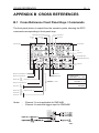
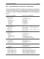
B.1 Cross Reference Front Panel Keys / Commands . . . . . . . . . . B-1
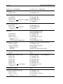
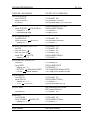
B.2 Cross Reference Softkey Menus / Commands . . . . . . . . . . . . B-3
B.2.1 ACQUIRE menu . . . . . . . . . . . . . . . . . . . . . . . . . . . . . . . . B-3
B.2.2 CURSORS menu . . . . . . . . . . . . . . . . . . . . . . . . . . . . . . . B-4
B.2.3 DISPLAY menu . . . . . . . . . . . . . . . . . . . . . . . . . . . . . . . . . B-5
B.2.4 MATHPLUS MATH menu . . . . . . . . . . . . . . . . . . . . . . . . . B-6
B.2.5 MEASURE menu . . . . . . . . . . . . . . . . . . . . . . . . . . . . . . . . B-9
B.2.6 DTB (DEL’D TB) menu . . . . . . . . . . . . . . . . . . . . . . . . . . . B-9
B.2.7 SAVE/RECALL menu . . . . . . . . . . . . . . . . . . . . . . . . . . . B-10
B.2.8 SETUPS menu . . . . . . . . . . . . . . . . . . . . . . . . . . . . . . . . B-10
B.2.9 TB MODE menu . . . . . . . . . . . . . . . . . . . . . . . . . . . . . . . B-11
B.2.10 TRIGGER menu . . . . . . . . . . . . . . . . . . . . . . . . . . . . . . . B-12
B.2.11 UTILITY menu . . . . . . . . . . . . . . . . . . . . . . . . . . . . . . . . . B-14
B.2.12 VERTICAL menu . . . . . . . . . . . . . . . . . . . . . . . . . . . . . . . B-16
B.3 Cross Reference Functions / Commands . . . . . . . . . . . . . . . B-17
C MANUAL CONVENTIONS
. . . . . . . . . . . . . . . . . . . . . . . . . . . . C-1
C.1 Abbreviations Used . . . . . . . . . . . . . . . . . . . . . . . . . . . . . . . . . . C-1
C.2 Glossary of Symbols Used . . . . . . . . . . . . . . . . . . . . . . . . . . . . C-4
C.3 List of Tables . . . . . . . . . . . . . . . . . . . . . . . . . . . . . . . . . . . . . . . . C-4
C.4 List of Figures . . . . . . . . . . . . . . . . . . . . . . . . . . . . . . . . . . . . . . . C-5
C.5 Documents Referenced . . . . . . . . . . . . . . . . . . . . . . . . . . . . . . . C-6
D STANDARDS INFORMATION
. . . . . . . . . . . . . . . . . . . . . . . . D-1
D.1 SCPI Conformance Information . . . . . . . . . . . . . . . . . . . . . . . . D-1
D.2 List of Implemented IEEE-488.2 Syntactical Elements . . . . . . D-2
E SUMMARY OF SYSTEM SETTINGS
. . . . . . . . . . . . . . . . . E-1
ABOUT THIS MANUAL
1-1
1 ABOUT THIS MANUAL
The SCPI Programming Manual for the CombiScope instruments describes
how to program your CombiScope instrument via the IEEE bus using SCPI
commands.
1.1 What this Manual Contains
A complete table of contents is given at the beginning of the manual.
Chapter 1
ABOUT THIS MANUAL
Explains what the SCPI programming manual for the CombiScopes
instruments contains.
Chapter 2
GETTING STARTED WITH SCPI PROGRAMMING
Tells you how to get started quickly with your CombiScope instrument.
You can execute the program examples per (sub)section or from the
beginning until the end.
Chapter 3
USING THE COMBISCOPE INSTRUMENTS
Explains how SCPI works for your CombiScope instrument from
the functional point of view. Section 3.1 is an introduction and
section 3.2 explains the fundamental programming concepts. The
other sections and subsections represent the functional use of your
CombiScope instrument.
Chapter 4
COMMAND REFERENCE
Is a complete alphabetical reference of all implemented SCPI
commands. In the beginning a command summary is given to
provide you with a quick reference.
1-2
ABOUT THIS MANUAL
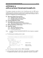
Appendix A
APPLICATION PROGRAM EXAMPLES
Appendix A describes some application program examples. The
application programs are supplied on floppy.
Appendix B
CROSS REFERENCES
Appendix B gives cross references between SCPI commands and
front panel keys, softkey menu options, and instrument functions.
Appendix C
MANUAL CONVENTIONS
Appendix C explains which abbreviations and symbols are used in
the manual. It also gives a list of the tables, figures, and documents
referenced.
Appendix D
STANDARDS INFORMATION
Appendix D gives information regarding SCPI and IEEE-488.2
standards.
Appendix E
SUMMARY OF SYSTEM SETTINGS
Appendix E lists the system settings per functional group (node),
plus the applicable instrument settings per node.
A full alphabetical index is given at the end of the manual.
GETTING STARTED WITH SCPI PROGRAMMING
2-1
2 GETTING STARTED WITH SCPI
PROGRAMMING
2.1 Preparations for SCPI Programming
To program your CombiScope instrument, you need a system setup and a
programming environment. Various program examples (refer to PROGRAM
EXAMPLE:) are given in the following sections. These program examples can be
executed one at a time or chained together for a complete tutorial. The program
examples are based on the system and programming environment as described
below.
Note:
All PROGRAM EXAMPLE's in this chapter are supplied on floppy under
the file name EXGETSTA.BAS. They are chained together in order of
appearance.
2.1.1
System setup
•
•
The CombiScope instrument contains a factory-installed IEEE option.
A PC is used as controller. In the PC an IEEE-488.2 interface (GPIB) board
must be installed to turn the PC into a GPIB controller. The GPIB controller
must be connected to the CombiScope instrument via an IEEE cable.
Note:
The program examples throughout this manual have been executed
on an IBM-compatible PC with the GPIB interface board and
software of the product PM2201/03 installed. The PM2201 board is
equivalent to the PCIIA board from National Instruments.
2.1.2
•
•
Programming environment
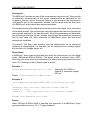
MS-QuickBASIC is used as the programming language.
A number of standard IEEE-488.2 drivers are used to control the CombiScope
instrument via the GPIB. These drivers must be included in the application
program. Therefore, the first statement of an application program must be as
follows:
REM $INCLUDE: ’<path>QBDECL.BAS’
Note:
The program examples throughout this manual have been executed
using the IEEE-488.2 drivers and the device handler GPIB.COM of
the product PM2201/03.
2-2
GETTING STARTED WITH SCPI PROGRAMMING
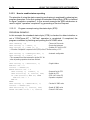
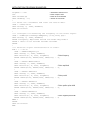
The parameters of these drivers are defined by the device handler GPIB.COM
and by the QuickBASIC program code. The following drivers and parameters are
used in the program examples:
•
The IEEE-488.2 driver "Send" is used to send a command or query to an
instrument.
CALL Send (<board>, <address>, <command>, <eot>)
•
The IEEE-488.2 driver "SendSetup" is used to prepare one or more devices
to receive data bytes. The controller becomes talker and the device becomes
listener.
CALL SendSetup (<board>, <addresslist>)
•
The IEEE-488.2 driver "SendDataBytes" is used to send data bytes from a
talking controller to a listening device.
CALL SendDataBytes (<board>, <data>, <eot>)
•
The IEEE-488.2 driver "Receive" is used to read a response string from an
instrument.
CALL Receive (<board>, <address>, <response>, <term>)
•
The IEEE-488.2 driver "SendIFC" is used to clear the GPIB interface.
CALL SendIFC (<board>)
•
The IEEE-488.2 driver "IbTMO" is used to specify a time out period for the
interface board.
CALL IbTMO (<board>, <timeout>)
Explanation of the parameters used in the IEEE-488.2 drivers:
•
<board>
IEEE board identification inside the PC (default board
address = 0).
•
<address>
IEEE instrument address (default CombiScope instrument
address = 8).
•
<addresslist>
Array containing GPIB device addresses, terminated by the
constant -1 (FFFF hex.).
•
<command>
A command or query string to be sent to the instrument. The
"short form" commands are specified in UPPER CASE. The
additional characters in lower case complete the "long form"
commands.
•
<data>
One or more data characters to be sent to the listener device.
GETTING STARTED WITH SCPI PROGRAMMING
2-3
•
<response>
A response string sent by the instrument as a response to a
query.
•
<eot>
An "end of text" indication:
0 = program message to be continued (no action)
1 = end of program message (sends End-message + EOI
true)
•
<term>
A "terminate" indication:
0 = response message to be continued (no detection of EOL
character)
256 = end of response message (stops reading after EOL
character)
•
<timeout>
A time out indication, e.g., 11 = 1 second, 12 = 3 seconds,
13 = 10 seconds.
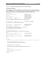
PROGRAM EXAMPLE:
’*****
’Initial program statements:
’*****
REM $INCLUDE:’c:\pc-gpib\488driv\QBDECL.BAS’
CLS
CALL SendIFC(0)
CALL IbTMO(0, 13)
’Includes GPIB drivers
’Clears text from PC screen
’Clears the GPIB interface
’Sets time out at 10 seconds
PROGRAMMING NOTE:
The variable IBCNT% contains the number of response bytes (including NL)
after reading a response message using the Receive driver.
2-4
GETTING STARTED WITH SCPI PROGRAMMING
2.2 Initializing the CombiScope Instrument
2.2.1
How to reset the CombiScope instrument
The instrument itself can be reset by sending the *RST command. This sets the
instrument to a fixed setup optimized for remote operation. The status and error
data of the instrument can be cleared by sending the *CLS command.
PROGRAM EXAMPLE:
’*****
’Reset the instrument and clear the status data:
’*****
CALL Send(0, 8, "*RST", 1)
’Resets the instrument
CALL Send(0, 8, "*CLS", 1)
’Clears the status data
2.2.2
How to identify the CombiScope instrument
The identity of the instrument can be queried by sending the *IDN? query,
followed by reading the instrument response message. The options of the
instrument can be queried by sending the *OPT? query, followed by reading the
instrument response message.
PROGRAM EXAMPLE:
’*****
’Read and print the identity and options of
’*****
response$ = SPACE$(65)
CALL Send (0, 8, "*IDN?", 1)
CALL Receive (0, 8, response$, 256)
PRINT "Ident: "; LEFT$(response$, IBCNT%)
CALL Send (0, 8, "*OPT?", 1)
CALL Receive (0, 8, response$, 256)
PRINT "Options: "; LEFT$(response$, IBCNT%)
2.2.3
the instrument:
’Requests for identification
’Reads the ident string
’Prints the ident string
’Requests for options
’Reads the options string
’Prints the options string
How to switch between digital and analog mode
After power on, a CombiScope instrument can be either in the digital or analog
mode. After a *RST command the digital mode is selected. The INSTrument subsystem allows you to switch between the two modes. This can be done by specifying a predefined name (DIGital, ANALog) or the corresponding number
(1 = digital, 2 = analog).
PROGRAM EXAMPLE:
’*****
’Initialize and change the operating mode of the CombiScope instrument:
’*****
CALL Send (0, 8, "INSTrument ANALog", 1)
’Switches to analog mode
CALL Send (0, 8, "INSTrument:NSELect 1", 1) ’Switches back to digital mode
GETTING STARTED WITH SCPI PROGRAMMING
2-5
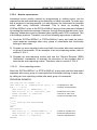
2.3 Error Reporting
Instrument errors are usually caused by programming or setting errors. They are
reported by the instrument during the execution of each command. To make sure
that a program is running properly, you must query the instrument for possible errors after every functional command. This is done by sending the
SYSTem:ERRor? query or the STATus:QUEue? query to the instrument, followed
by reading the response message. However, through this practice the same "error
reporting" statements must be repeated after sending each SCPI command. This
is not always practical. Therefore, one of the following approaches is advised:
1) Send the SYSTem:ERRor? or STATus:QUEue? query and read the instrument
response message after every group of commands that functionally belong to
each other.
2) Program an error-reporting routine and call this routine after each command
or group of commands. For an example of an error-reporting routine, refer to
section 3.14.4.1.
3) Program an error-reporting routine and use the "Service Request (SRQ)
Generation" mechanism to interrupt the execution of the program and to
execute the error-reporting routine. Therefore, refer to section 3.14.4.2.
PROGRAM EXAMPLE:
’*****
’Read error message:
’*****
er$ = SPACE$(60)
CALL Send(0, 8, "SYSTem:ERRor?", 1)
CALL Receive(0, 8, er$, 256)
PRINT "Response to error query = ";
PRINT LEFT$(er$, IBCNT%-1)
’Requests for error
’Reads error message
’Displays error message
2-6
GETTING STARTED WITH SCPI PROGRAMMING
2.4 Acquiring Traces
Trace acquisitions are started via the INITiate commands. A single acquisition is
done by sending a single INITiate command. Continuous acquisitions are done by
sending the INITiate:CONTinuous ON command.
The TRACe? query allows you to acquire a trace of signal samples from one of
the following sources:
•
•
An input channel, e.g., CH2 (input channel 2).
A trace area in a memory register, e.g., M2_3 (Memory register 2, trace 3).
The number of trace samples (acquisition length) can be specified using the
TRACe:POINts command. If your instrument has standard memory, you can
specify 512, 2048, 4096, or 8192 trace samples. If your instrument has extended
memory, you can specify 512, 8192, 16384, or 32768 trace samples. A
TRACe:POINts command specifies the acquisition length for all channels and
memory registers.
Example: Send --> TRACe:POINts CH1,8192 ’Selects 8192 sample points
for all traces
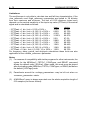
The number of trace sample bits can be specified using the FORMat command.
This gives you the possibility to define samples of 8 bits (1 byte) or 16 bits
(2 bytes). A FORMat command specifies the number of sample bits for all
channels and memory registers.
Example: Send --> FORMat INT,16
’Formats 16-bits samples
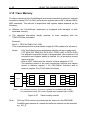
The format of the trace response data is as follows:
# n x . . x f b . . . . . b s < NL>
NewLine code (10 decimal)
checksum byte over all trace bytes
trace sample data bytes (see Note)
trace data format byte (see Note)
number of trace bytes (fbb...bbs)
number of digits of x..x
Note:
If f=8 decimal, each trace sample is one byte (8 bits).
If f=16 decimal, each trace sample is two bytes (16 bits), i.e., most significant byte
(msb) + least significant byte (lsb).
Example:
# 4 1 0 2 6 <16> <msb 1> <lsb 1> . . . <msb 512> <lsb 512> <checksum> <10>
trace sample 512
trace sample 1
decimal 16
number of trace bytes (N)
number of digits of N
GETTING STARTED WITH SCPI PROGRAMMING
2.4.1
2-7
How to acquire a single shot trace
In the program example, a single shot trace acquisition of 8192 8-bit samples is
done with a probe connected to input channel 1. The trace sample bytes are read
from the GPIB as string characters. The number of response bytes and the
number of samples are printed.
The TRIGger:SOURce command is used to specify input channel 1 as a trigger
source. The TRIGger:LEVel command is used to reset the trigger level to e.g., 0.1
volts.
PREPARATIONS:
•
Connect a probe to channel 1. After start up of the program you will be asked
to trigger the acquisition with the open end of the probe, i.e., touch the probe
or strike the probe on the table.
PROGRAM EXAMPLE:
’*****
’Acquire a single shot trace:
’*****
DIM tracebuf AS STRING * 16500
CALL Send(0, 8, "FORMat INTeger,8", 1)
’Formats 8-bits sample
CALL Send(0, 8, "TRACe:POINts CH1,8192", 1)
’Formats 8192 sample points
CALL Send(0, 8, "TRIGger:SOURce INTernal1", 1) ’Trigger-source = channel 1
CALL Send(0, 8, "TRIGger:LEVel 0.1", 1)
’Trigger-level = 0.1
CALL Send(0, 8, "INITiate", 1)
’Single shot initiation
PRINT "Trigger the CombiScope instrument by touching the probe tip."
PRINT ">>> Press any key when finished."
WHILE INKEY$ = "": WEND
CALL Send(0, 8, "*WAI", 1)
’Waits for previous commands
to finish
CALL Send(0, 8, "TRACe? CH1", 1)
’Queries for channel 1 trace
CALL Receive(0, 8, tracebuf$, 256)
’Reads channel 1 trace
’
’The contents of the tracebuf$ string is as follows:
’# 4 8194 <8> <byte 1> ... <byte 8192> <sum> <10>
’
nr.of.digits = VAL(MID$(tracebuf$, 2, 1))
nr.of.bytes = VAL(MID$(tracebuf$, 3, nr.of.digits)) - 2
sample.length = ASC(MID$(tracebuf$, 3 + nr.of.digits, 1)) / 8
nr.of.samples = nr.of.bytes / sample.length
PRINT "Number of bytes received ="; IBCNT%
’IBCNT% = number of bytes
PRINT "Number of trace samples ="; nr.of.samples
Note:
Refer to section 3.4.3 "Conversion of trace data" about how to convert
this string data.
2-8
2.4.2
GETTING STARTED WITH SCPI PROGRAMMING
How to acquire repetitive traces
In the program example, 5 trace acquisitions of 512 16-bit samples are done via
a probe connected to channel 2. The trace sample bytes are read from the GPIB
as string characters and written to the file TRACE5.DAT on the hard disk.
PREPARATIONS:
•
Connect a probe from the Probe Adjust signal to channel 2.
PROGRAM EXAMPLE:
’*****
’Acquire 5 sequential traces and store in file TRACE5.DAT:
’*****
DIM tracebuf AS STRING * 1050
CALL Send(0, 8, "*RST", 1)
’Resets the instrument
’
’After *RST a trace acquisition is defined at 512 samples of 16 bits
’(2 bytes).
’
CALL Send(0, 8, "CONFigure:AC (@2)", 1)
’Configures channel 2
CALL Send(0, 8, "SENSe:FUNCtion ’XTIMe:VOLTage2’", 1)’Switches channel 2 on
OPEN "O",#1,"TRACE5.DAT"
’Opens file TRACE5.DAT
FOR i=1 TO 5
CALL Send(0, 8, "INITiate", 1)
’Single initiation
CALL Send(0, 8, "*WAI;TRACe? CH2", 1)
’Queries for channel 2 trace
’
’Notice the *WAI; before TRACe?. The *WAI command takes care that the TRACe? CH2 command is
’executed when the INITiate command is finished.
’
CALL Receive(0, 8, tracebuf$, 256)
’Reads channel 2 trace
PRINT #1, "Trace buffer:"; i
’Writes trace header to file
PRINT #1, LEFT$(tracebuf$, IBCNT%)
’Writes trace buffer to file
NEXT i
CLOSE
’Closes file TRACE5.DAT
Note:
Refer to section 3.4.3 "Conversion of trace data" about how to convert
this string data.
GETTING STARTED WITH SCPI PROGRAMMING
2-9
2.5 Measuring Signal Characteristics
The measurement instructions allow you to make a complete measurement. This
includes the configuration of the instrument, the initiation of the trigger system,
and the fetching of the acquisition data. The measurement instructions can be
used at different levels, varying in processing time. The highest level is the most
easy to use, but takes more time to complete than the lowest level. The following
levels of measurement instructions can be used:
The highest level:
(easy to use)
MEASure?
The middle level:
CONFigure + READ?
(gives more programming flexibility)
(equivalent to MEASure?)
The lowest level:
INITiate + FETCh?
(to acquire more signal characteristics)
(equivalent to READ?)
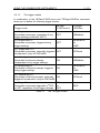
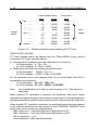
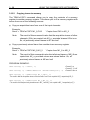
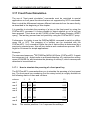
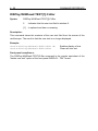
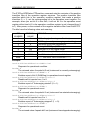
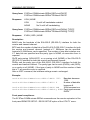
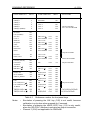
The following table shows which measurement tasks are executed by the
measurement instructions:
MEASure? CONFigure
Configures the instrument:
YES
READ?
INITiate
YES
FETCh?
YES
Initiates the trigger system:
YES
YES
Fetches the acquired data:
YES
YES
YES
2 - 10
2.5.1
GETTING STARTED WITH SCPI PROGRAMMING
How to make a single shot measurement
The MEASure? query allows you to make a single-shot measurement, and the
FETCh? query allows you to fetch more signal characteristics.
PROGRAM EXAMPLE:
’*****
’Measure and print the AC-RMS, peak to peak, and amplitude of
’the signal on channel 1.
’*****
response$ = SPACE$(30)
CALL Send (0, 8, "MEASure:AC? (@1)", 1)
’Measures the AC-RMS value
CALL Receive (0, 8, response$, 256)
’Reads the AC-RMS value
PRINT "AC-RMS value
: "; LEFT$(response$, IBCNT% -1)
CALL Send (0, 8, "FETCh:PTPeak?", 1)
’Fetches the Peak-To-Peak value
CALL Receive (0, 8, response$, 256)
’Reads the PTP value
PRINT "Peak-To-Peak value: "; LEFT$(response$, IBCNT% - 1)
CALL Send (0, 8, "FETCh:AMPLitude?", 1)
’Fetches the amplitude value
CALL Receive (0, 8, response$, 256)
’Reads the amplitude value
PRINT "Amplitude value
: "; LEFT$(response$, IBCNT% - 1)
2.5.2
How to make repeated measurements
The measurement instructions allow you to make repeated measurements. The
CONFigure command allows you to configure the instrument, the READ? query
allows you to make a measurement, and the FETCh? query allows you to fetch
more signal characteristics.
PROGRAM EXAMPLE:
’*****
’Measure and print 5x the AC-RMS, peak to peak, and
’amplitude of the signal on channel 1.
’*****
response$ = SPACE$(30)
CALL Send (0, 8, "CONFigure:AC (@1)", 1)
’Configures for AC-RMS
FOR i = 1 TO 5
’Performs 5 measurements
CALL Send (0, 8, "READ:AC?", 1)
’Initiates AC-RMS reading
CALL Receive (0, 8, response$, 256)
’Reads the AC-RMS value
PRINT "AC-RMS: "; LEFT$(response$, IBCNT%-1);
CALL Send (0, 8, "FETCh:PTPeak?", 1)
’Fetches the Peak-To-Peak value
CALL Receive (0, 8, response$, 256)
’Reads the PTP value
PRINT " / Peak-To-Peak: "; LEFT$(response$, IBCNT%-1);
CALL Send (0, 8, "FETCh:AMPLitude?", 1)
’Fetches the amplitude value
CALL Receive (0, 8, response$, 256)
’Reads the amplitude value
PRINT " / Amplitude: "; LEFT$(response$, IBCNT%-1)
NEXT i
USING THE COMBISCOPE INSTRUMENTS
3-1
3 USING THE COMBISCOPE
INSTRUMENTS
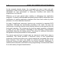
3.1 Introduction
This chapter explains how to access the functions of the CombiScope instruments
family in a remote programming environment. For that purpose, the CombiScope
instrument is equipped with an IEEE-488 compatible GPIB interface and
implements a full SCPI compatible command set which provides an extensive
range of remote control facilities.
Traditionally, there was no standard for the remote operation of instruments. A
wide range of different command sets existed. Each set had its own terminology
and trade-offs, based upon the implementations and corresponding limitations of
the instrument. Similar functions in different instruments were controlled by
different commands. And, vice versa, identical commands could easily exist in
another instrument to control a different function. With new technologies and
increasing complexity, other programming concepts were introduced. This caused
programs with identical functions to look different when written for another
instrument.
The remote control of instruments became a cumbersome process, which
required a high learning curve for each new instrument and each additional
instrument. The time and costs to create and maintain application programs were
unnecessarily high due to the lack of standardization.
With the introduction of the Standard Commands for Programmable Instruments,
commonly called SCPI, a lot of progress has been made in this area. The
development time of an application program for SCPI-compatible instruments, like
the CombiScope instrument, is considerably reduced. This is mainly achieved by
the consistent programming environment for instrument control and data usage
across all types of instruments that, regardless of the manufacturer, is provided by
SCPI.
The standardized commands allow the same functions in different types of
instruments to be controlled by the same commands. For example, the query
MEASure:FREQuency? acquires the frequency characteristic of the input signal,
regardless of whether the instrument is a frequency counter, an oscilloscope, or
any other measuring instrument.
3-2
USING THE COMBISCOPE INSTRUMENTS
As the example already shows, the commands are easy to learn and selfexplanatory to both novice and expert users. The learning curve is considerably
decreased for new instruments or instrument functions with which the
programmer is not familiar.
Efficiency is not only gained when creating or debugging new application
programs. The easily understandable programs greatly simplify maintenance and
modification of existing application programs that have been written by other
persons or for other instrument functions.
All major CombiScope instrument functions are controlled by standard SCPI
commands. Although the functionality provided is the same, the way the
oscilloscope is controlled via the remote interface differs in some aspects from the
front panel operation. This is because the local front panel operation is designed
to allow you to take maximum advantage of the interactive communication
possibilities offered by the display screen. This allows for additional information
and guidance during the process of local operation.
The remote command set is based upon an instrument model that is easy to
understand. This model provides a structured survey of the implemented
instrument functions and serves as a guide towards the commands that control
these functions. This other view allows for optimal and easy access of the
instrument functions when operated from the remote interface. Additionally, a
measurement instruction set allows for easy programming of measurement tasks
for a wide variety of signal characteristics.
USING THE COMBISCOPE INSTRUMENTS
3-3
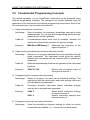
3.2 Fundamental Programming Concepts
The remote operation of your CombiScope instrument can be accessed using
different programming concepts. The concept to be chosen depends upon the
application of the instrument in the remote programming environment. Each of the
four concepts has it own benefits and trade-offs.
1) Using measurement instructions
Advantage:
Easy to program. No instrument knowledge required to make
measurements. So, you can start programming quickly and get
measurement results rightaway.
Trade-off:
A measurement takes some time to complete, because the
instrument automatically searches for optimal settings.
Example:
MEASure:FREQuency?
Measures the frequency of the
signal at channel 1.
2) Single function programming using the instrument model
Advantage:
Allows you to program individual functions separately through
single commands. The instrument model gives the relation
between the commands and the functions of the CombiScope
instrument.
Trade-off:
Requires understanding of the remote operation of the instrument
functions.
Example:
TRACe? CH1
Returns the acquisition trace of
the signal at channel 1.
3) Programming the complete instrument setup
Advantage:
Simple to program. No worry about individual settings. This
method can also be used to save and recall settings, which are
not individually programmable.
Trade-off:
Processes complete instrument setups. Individual settings
must be set or programmed separately.
Example:
*SAV 3
*RCL 3
Saves actual instrument settings
to internal memory 3.
Recalls instrument settings from
internal memory 3.
4) Programming through front panel simulation
Advantage:
Gives the possibility to program settings for which no remote
commands are available, i.e., to match a front panel setup.
3-4
USING THE COMBISCOPE INSTRUMENTS
Trade-off:
This way of programming is cumbersome and tricky, because
additional information on the front panel display is not always
available remotely.
Example:
DISPlay:MENU TRIGger
Activates the TRIGGER softkey
menu.
SYSTem:KEY 4
Simulates the pressing of softkey 4.
The effect is that TRIGGER menu
option "noise" is switched on or
off.
3.2.1
Measurement instructions
This is a completely new approach in the remote operation of programmable
instruments, which provides a set of task-oriented measurement instructions.
Rather than programming every instrument setting separately with starting the
acquisition and calculating the result, just specify the desired signal characteristic,
and the CombiScope instrument returns the requested result. Depending upon
the actual available signal, your CombiScope instrument automatically
determines the optimal settings to acquire and calculate the requested result.
An example of such a command is the MEASure:FREQuency? query, which not
only works on oscilloscopes, but also on different types of SCPI-compatible
instruments, such as counters and multimeters.
With traditional oscilloscopes you had to do the following:
-
set up all functions of the oscilloscope separately.
start the acquisition of the data.
position the cursor markers.
calculate the frequency from the acquired data.
read the calculated frequency from the instrument.
A single, simple SCPI query replaces all of the above, namely the
MEASure:FREQuency? query which does the following:
-
-
auto configures the oscilloscope to the best possible setting for the requested
measurement task.
Note:
This process is different from the traditional AUTOSET process in
that the autoset function determines the instrument settings based
on the input signal only, whereas, the auto configure algorithm also
takes the desired measurement task into account.
starts the acquisition process.
takes care that the measurement is triggered.
calculates the desired characteristic from the acquired data.
returns the calculated value.
USING THE COMBISCOPE INSTRUMENTS
3-5
The measurement instructions are easy to use and do not require any special
knowledge of the instrument. The programming concept reduces simple
measurement tasks with complex instruments to simple instructions, leaving the
setup complexity to the instrument. The measurement instructions are extremely
useful when the application does not require the precise setting of instrument
functions. The concept is extendible with separate control of parameters that are
vital to the application.
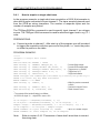
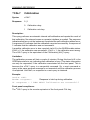
3.2.2
Single function programming using the instrument model
All major instrument functions such as time base, input impedance, etc, are
separately programmable using "single parameter" commands. The easy to
understand command set is comparable with the way instruments are traditionally
controlled. This concept gives you full control over all functions and power of a
modern oscilloscope. However, for maximum benefit of all the advanced features
of your CombiScope instrument, you need some understanding of their remote
operation.
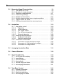
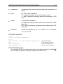
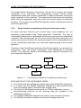
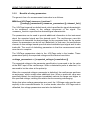
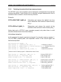
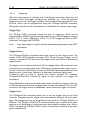
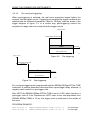
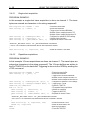
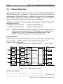
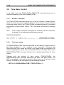
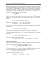
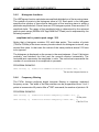
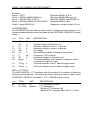
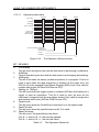
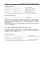
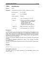
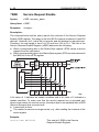
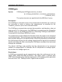
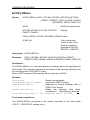
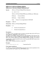
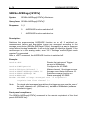
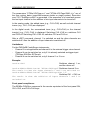
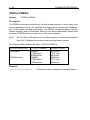
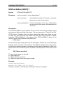
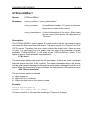
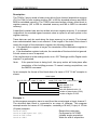
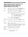
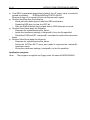
Functions of the CombiScope instrument that belong together are grouped into
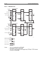
subsystems. There are several subsystems, each representing a particular
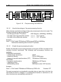
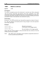
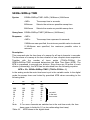
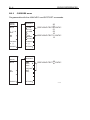
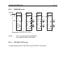
function. The instrument model in the following figure gives an overview of the
most important subsystems.
DISPlay
INPut
SENSe
TRACe
CALCulate
TRIGger
ST7155
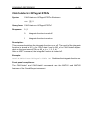
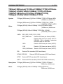
Figure 3.1
The Instrument Model for CombiScope instruments
EXPLANATION OF THE INSTRUMENT MODEL:
All functions that deal with signal conditioning are part of the INPut subsystem.
In a similar way the SENSe subsystem contains the data acquisition part
where the analog signal is converted into a digital value.
The results of the acquisition are stored in a TRACe subsystem memory.
Post-processing functions on the acquired data are available in the
CALCulate subsystem.
The TRIGger subsystem deals with the control of the acquisition process.
The DISPlay subsystem handles the front panel display functions.
•
•
•
•
•
•
3-6
USING THE COMBISCOPE INSTRUMENTS
Functions in a particular subsystem are always controlled by commands that
begin with the name of that subsystem. For example, a command that programs
the input coupling is INPut:COUPling DC.
All programmable settings can be queried easily. The query form is obtained from
the command by simply removing the parameter and adding a question mark. For
example, the command to program the input impedance of your oscilloscope is
INPut:IMPedance 50. This impedance value can be queried by sending
INPut:IMPedance? which returns 50.
3.2.3
Instrument setup
This concept allows you to program instrument settings with a single command.
Several instrument setups can be saved, either created by remote programming
or by front panel control. This concept can also be used to program instrument
functions that cannot be directly accessed using individual program instructions.
Complete instrument setups can be saved either in the internal memory of the
oscilloscope or externally in the remote controller. A part of the instrument setup
can also be saved externally.
The oscilloscope is equipped with a number of internal memories in which the
complete instrument set up can be saved and from which it can be restored.
Send → *SAV 3
Send → *RCL 3
Saves the current set up into memory 3.
Recalls the instrument set up that was saved in memory 3.
Instead of using an internal oscilloscope memory, the instrument setup can be
queried using the SYSTem:SET? query. The result of this query is that the
oscilloscope sends a part or the complete setup in a compact block data format.
Sending this data back as a parameter with the SYSTem:SET command
reprograms the oscilloscope to the same settings.
Example for the complete instrument settings:
Send → SYSTem:SET?
Read ← <block_data>
Send → SYSTem:SET <block_data>
Queries the oscilloscope for the complete
instrument setup.
Reads the <block_data> response, which
contains the requested instrument setup,
from the oscilloscope.
Sends the previously read instrument
setup back to the oscilloscope in the
same <block_data> format.
USING THE COMBISCOPE INSTRUMENTS
3-7
Example for the instrument cursor settings:
Send → SYSTem:SET? 32
Queries the oscilloscope for the
instrument settings of node 32, which are
the cursor settings.
Read ← <settings>
Reads the cursor settings.
.
.
Send → SYSTem:SET <settings>
3.2.4
Restores the cursor settings.
Front panel simulation
This concept allows you to send commands that simulate the pressing of a front
panel key. This method allows the remote operation to precisely match a front
panel setup. In particular, this method can be used to access instrument functions
that cannot be programmed directly by remote commands.
As described in the beginning of this section, there is a difference between the
front panel operation and the remote control of an instrument. If you use the front
panel simulation commands via the remote interface, be aware that no use can
be made of the additional information that is presented on the screen of the
oscilloscope. As this causes the front panel simulation method to be a tedious
process, it is certainly not recommended as a common programming practice.
For example, the SYSTem:KEY 507 command switches the AVERAGE function
on when it was switched off before. When this function was switched on before,
the AVERAGE function is switched off. The effect of the SYSTem:KEY command
completely depends upon the state of the instrument at the moment the command
is received. In a remote programming environment it is not immediately clear
whether a state is on or off. For that reason the command SENSe:AVERage ON
is much better.
To select functions that cannot be programmed directly, you might use the front
panel simulation commands. For example, the command SYSTem:KEY 4
switches the "noise suppression" option in the TRIGGER menu of the front panel
ON or OFF.
3-8
USING THE COMBISCOPE INSTRUMENTS
3.3 Measuring Signal Characteristics
As explained in section 3.2.1 "Measurement instructions", the measurement
instruction set is a new approach in the remote operation of programmable
instruments. This instruction set allows you to request a particular characteristic
of the input signal. The CombiScope instrument then chooses the best possible
settings, executes the requested task, and returns the desired result.
Within the measurement instruction set, different programming levels can be
distinguished. The highest level is the easiest to use, but the trade-off is less
flexibility. Lower levels provide more flexibility by offering more control over the
instrument functionality. This requires more knowledge about the remote
operation of your instrument.
The measurement instructions specify a particular task in terms of the expected
signal and the desired result. The instructions refer to the signal characteristics of
the signal being measured. This makes them independent from the
implementation of the instrument functions. For example, when the instruction
MEASure:FREQuency? is executed, it is not important whether this frequency is
measured by precisely counting the signal period, or if it is calculated from a
sampled waveform. For this reason, the measurement instructions provide the
best compatibility among different types of instruments. But, as a trade-off, the
compatibility decreases when more flexibility is needed and lower measurement
instruction levels are used.
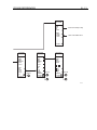
3.3.1
The MEASure? query
This is the easiest instruction to use and provides the best compatibility. However,
it does not offer access to the full capability of the CombiScope instrument. The
MEASure? query configures the instrument for optimal settings, starts the data
acquisition, and returns the result in one operation. The signal characteristics that
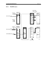
can be acquired in this way are shown in figure 3.2.
Example:
MEASure:AC?
This query measures the RMS voltage of the AC component at the default
input channel 1. After the acquisition, the result is sent to the controller. The
instrument itself selects an optimal setting for this purpose and carries out the
requested measurement as "well" as possible. Moreover, it automatically
starts the measurement.
USING THE COMBISCOPE INSTRUMENTS
3.3.2
3-9
Benefits of using parameters
The generic form of a measurement instruction is as follows:
MEASure[:VOLTage]:<measure_function>?
[[<voltage_parameters>,]<measure_parameters>][,<channel_list>]
The :VOLTage keyword is a default node, which specifies the signal characteristic
to be measured, relates to the voltage component of the signal. The
<measure_function> specifies the desired signal characteristic.
The parameters can be used to provide additional information to the instrument
about the expected signal and the desired result. The oscilloscope uses this
information to determine the best settings for the requested task. As the syntax
shows, the parameters can be left out (defaulted). In that case, the oscilloscope
chooses it own settings based upon the actual available input signal and its own
trade-offs. The result of defaulting parameters is that the measurement needs
more time to complete.
The VOLTage parameters relate to the :VOLTage node in the header. These
parameters specify the expected voltage and the desired resolution:
<voltage_parameters> = [<expected_voltage>[,<resolution>]]
The expected voltage in the parameter specification is assumed to be the value
at the BNC input of the oscilloscope. When a detectable probe is attached, it is
assumed to be the value at the probe tip.
When the <expected voltage> parameter is defaulted, the oscilloscope performs
an autorange, which needs some additional time. When a particular value was
specified instead, the oscilloscope immediately selects the range next higher to
the specified voltage, omitting the relative time-consuming autoranging.
Notice that when voltage parameters are used, the :VOLtage node must be sent
explicitly in the command header. Or, in other words, when the :VOLTage node is
defaulted, the voltage parameters must also be defaulted.
3 - 10
USING THE COMBISCOPE INSTRUMENTS
Examples:
MEASure:AMPLitude?
This query measures the amplitude of a waveform at the default input
channel 1. After the acquisition, the resulting amplitude is returned.
MEASure:VOLTage:AMPLitude? 10, (@2)
This query measures the amplitude of a signal at channel 2 (@2). But, since
it specifies the expected voltage value (10 volts), it will complete the
measurement faster.
In a similar way the measure function parameters provide the oscilloscope with
information about the signal characteristic to be measured. The parameters that
are allowed depend upon the requested signal characteristic (measure function).
The measure function parameters that specify a voltage characteristic, such as
:AC, :AMPLitude, :HIGH, :MINimum, etc, use the voltage parameters for that
purpose. Measure functions, such as fall and rise time, frequency and period, use
time units. Their expected value and desired resolution are specified in seconds
or Hertz as separate measure parameters.
Examples:
MEASure:VOLTage:FREQuency? 10E6, (@3)
This query measures the frequency of the signal at input channel 3. The
expected frequency is 10 MHz, whereas, the expected voltage is defaulted.
Notice that this command is equivalent to the MEASure:FREQuency? 10E6,
(@3) command.
MEASure:VOLTage:FREQuency? 5, 10E6, (@3)
This query does the same as the previous example, except that the expected
voltage is 5 volts.
USING THE COMBISCOPE INSTRUMENTS
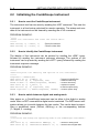
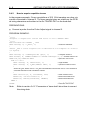
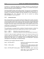
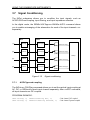
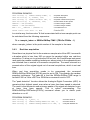
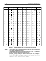
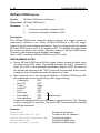
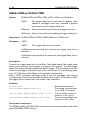
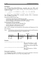
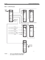
3.3.3
3 - 11
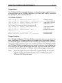
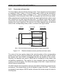
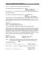
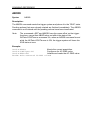
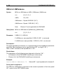
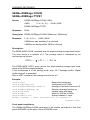
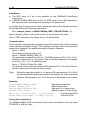
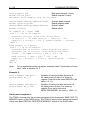
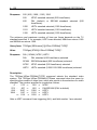
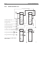
Waveform measurements
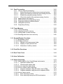
The following figure shows the terms used for pulse measurements and the key
words that are used as header nodes in the measurement instructions.
TMAXimum
MAXimum
HIGH
RISE
OVERshoot
RISE TIME
FALL TIME
FALL
PREShoot
PTPeak
AMPLitude
REFerence
HIGH
REFerence
MIDDle
REFerence
LOW
LOW
RISE
PREShoot
FALL
OVERshoot
MINimum
TMINimum
PWIDth
NWIDth
PERiod
Figure 3.2
ST7154
Pulse characteristics
The reference high and low parameters determine the desired interval for rise
time and fall time measurements. The default low and high references are 10%
and 90% of the pulse amplitude (= HIGH - LOW).
Default REFerence LOW =LOW + 0.1 * (HIGH - LOW)
Default REFerence HIGH =LOW + 0.9 * (HIGH - LOW)
In a similar way, the reference middle parameter determines the desired interval
for pulse width (PWIDth, NWIDth) and duty cycle (PDUTycycle, NDUTycycle)
measurements. When defaulted, the reference middle value is assumed to be at
50% of the amplitude.
Default REFerence MIDDle =LOW + 0.5 * (HIGH - LOW)
3 - 12
USING THE COMBISCOPE INSTRUMENTS
Examples:
MEASure:FALL:TIME? (@3)
Measures the time interval during which the pulse at channel 3 decreases
from 90% to 10% of its amplitude.
MEASure:RISE:TIME? 20,80
Measures the time interval during which the pulse at the default channel 1
increases from 20% to 80% of its amplitude.
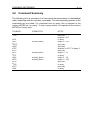
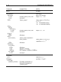
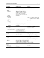
The following measure functions and parameters can be programmed:
<measure_function><measure_parameters>
:AC
:AMPLitude
[:DC]
:FALL
:OVERshoot
:PREShoot
:TIME
[<reference_low> [,<reference_high> [,<expected_time>
[,<time_resolution>]]]]
:FREQuency
[<expected_frequency> [,<frequency_resolution>]]
:HIGH
:LOW
:MAXimum
:MINimum
:NDUTycycle
<reference_middle>
:NWIDth
<reference_middle>
:PDUTycycle
<reference_middle>
:PERiod
[<expected_period> [,<period_resolution>]]
:PTPeak
:PWIDth
<reference_middle>
:TMAXimum
:TMINimum
:RISE
:OVERshoot
:PREShoot
:TIME
[<reference_low> [,<reference_high> [,<expected_time>
[,<time_resolution>]]]]
Notes:
- :DCYCle = alias for :PDUTycycle
- :FTIMe = alias for :FALL:TIME
- :RTIMe = alias for :RISE:TIME
USING THE COMBISCOPE INSTRUMENTS
3.3.4
3 - 13
Customizing settings
Often, you need more precise control of the measurements than possible with the
MEASure? query. The combination of CONFigure and READ? is provided to
allow you to program one or more settings that are vital to your application.
Executing this sequence of instructions is equivalent to sending MEASure? For
setting up the instrument, CONFigure uses the same measure functions and
parameters as MEASure?. The CONFigure command does the instrument setup
portion of MEASure?. The READ? query initiates the acquisition, performs the
needed calculations, and returns the desired result.
Since READ? no longer changes instrument settings, commands that are
executed after CONFigure, but before READ?, are taken into effect by the
acquisition. This concept allows you to perform a generic configuration through
CONFigure and then customize the measurement by programming the settings
that are vital to your application. Next the READ? completes the measurement
process.
Example:
CONFigure:AC
Configures the instrument to perform an RMS
measurement of the AC component at the default
input channel 1.
SENSe:AVERage ON
Sets averaging on.
SENSe:AVERage:COUNT 4 Sets averaging factor at four.
READ:AC?
Starts the measurement and returns the averaged
AC-RMS value.
READ? uses the same measure functions and parameters as CONFigure. After
the instrument has been set up for a particular measure function by the
CONFigure command, the same measure function key words can be repeated by
the READ? query header. Moreover, it is allowed to request for another signal
characteristic by specifying a measure function other than that for which the
instrument was configured. However, keep in mind that the instrument was set up
by CONFigure for another task. As these settings are not affected by READ?, it
is not guaranteed that the instrument is able to acquire the signal characteristic
that is requested by READ?
Example:
CONFigure:AC
Sets up the instrument to perform an RMS
measurement of the AC component.
3 - 14
USING THE COMBISCOPE INSTRUMENTS
READ?
Requests to execute the default DC measurement.
Since this is not possible with the chosen
configuration, an execution error is generated and
no result is returned.
CONFigure:RISE:TIME
Configures the CombiScope instrument to perform a
rise time measurement.
READ:RISE:OVERshoot? Requests to read the rise time overshoot. Because the
CombiScope instrument is able to calculate the rise
overshoot value when it is set up for a rise time
measurement, the desired result is calculated and
returned.
A READ? also allows the same parameter sets as the corresponding CONFigure
instructions. But, these sets only serve to specify the desired result. They are
ignored as far as they affect instrument settings. The parameters can be sent for
compatibility with the preceding CONFigure command.
Example:
CONFigure:RISE:TIME
Configures the oscilloscope to perform a default rise
time measurement (10% to 90% increase of the
signal amplitude).
READ:RISE:TIME? 20,80
Requests for the rise time of the 20 to 80% increase
of the signal amplitude. As the CombiScope
instrument is able to respond to this request, the
desired rise time is calculated and returned.
3.3.5
Multiple measurements
Sometimes it is necessary to perform multiple measurements of the same signal
characteristic. This can be realized by executing multiple MEASure? queries.
However, this implies that the relative time-consuming configuration portion of
MEASure? is unnecessarily repeated. This can be easily avoided by using the
CONFigure and READ? concept as described in the preceding chapter. This
concept allows you to do the configuration only once by sending the CONFigure
command one time. Sending multiple READ? queries next, causes the instrument
to repeatedly execute the desired measurement.
Example:
CONFigure:FREQuency
Configures the instrument to perform a frequency
measurement.
USING THE COMBISCOPE INSTRUMENTS
3 - 15
READ:FREQuency?
Starts the acquisition and returns the measured
frequency.
READ:FREQuency?
Starts a next acquisition and returns the new
frequency result.
READ:FREQuency?
Etc.
3.3.6
Multiple characteristics from a single acquisition.
It is often necessary to determine several signal characteristics from the last
acquired waveform. Starting a new acquisition, as READ? and MEASure? do, is
undesired. For that purpose, READ? is broken down into two additional
instructions, which are the INITiate[:IMMediate] command and the FETCh? query.
Executing this sequence of instructions is equivalent to READ?. The
INITiate[:IMMediate] command starts the acquisition. FETCh? determines the
requested signal characteristic and returns the result. This concept allows you to
perform several different FETCh? queries on a single set of acquisition data.
Example:
MEASure:AC?
Configures the instrument to measure the RMS value
of the AC component of the signal at input channel 1,
starts the acquisition, and returns the desired result.
FETCh:FREQuency?
Determines and returns the frequency of the signal
that is acquired by the preceding MEASure? query.
FETCh:RISE:TIME?
Uses default parameters to determine and return the
rise time of the first pulse.
As distinct from the READ? query, defaulting the measure function part of the
FETCh? query, causes the CombiScope instrument to return the characteristic
that was requested with the last executed FETCh?, READ? or MEASure? query.
For this reason, the measure function should always be explicitly specified in the
header of the FETCh? query.
3 - 16
3.3.7
USING THE COMBISCOPE INSTRUMENTS
Trigger control via GPIB
You need a separate GPIB command to start a measurement synchronized with
other instruments. This is done by sending the *TRG command or the GET
(Group Execute Trigger) code. The MEASure? and READ? queries do not allow
you to do so, because such a setup causes a query error. With the
INITiate[:IMMediate] and FETCh? concept, it is possible to meet the requirements
of such applications.
Example:
CONFigure:AC
Configures the instrument to measure the AC-RMS
voltage.
TRIGger:SOURce BUS
Specifies that the acquisition is to be triggered by
GET or *TRG.
INITiate
Starts the measurement process.
*TRG
Triggers the acquisition.
FETCh:AC?
Determines and returns the AC-RMS value.
USING THE COMBISCOPE INSTRUMENTS
3.3.8
3 - 17
Fetching characteristics from memory traces
The FETCh? query not only allows you to determine a characteristic from the last
acquired waveform, it also allows you to calculate a signal characteristic from a
waveform that is stored in a trace memory element.
Example:
FETCh:RISE:TIME? (@M3_4)
Calculates and returns the default rise time
from a waveform that is stored in trace memory
M3_4.
FETCh:PERiod? (@M4_1)
Determines and returns the period of the
waveform that is stored in trace memory M4_1.
Notice that such a FETCh? query operates properly only when there is valid
waveform data stored in the trace memory.
PROGRAM EXAMPLE:
In this example the signal acquired via channel 2 is stored in memory register 1.
The AC-RMS, peak-to-peak, and amplitude values of the stored signal are
fetched and printed.
DIM response AS STRING * 10
CALL Send(0, 8, "CONFigure:AC (@2)", 1)
’Configures for channel 2
CALL Send(0, 8, "SENSe:FUNCtion ’XTIMe:VOLTage2’", 1)’Switches channel 2 on
CALL Send(0, 8, "INITiate", 1)
’Single initiation
CALL Send(0, 8, "TRACe:COPY M1_2,CH2", 1)
’Copies CH2-trace to M1_2
’
’Now trace area 2 of memory register 1 is filled with the channel 2 trace.
’
CALL Send(0, 8, "FETCh:AC? (@M1_2)", 1)
’Fetches AC-RMS of M1_2
CALL Receive(0, 8, response$, 256)
’Enters AC-RMS value
PRINT "AC-RMS value : "; response$
’Prints AC-RMS value
CALL Send(0, 8, "FETCh:PTPeak? (@M1_2)", 1)
CALL Receive(0, 8, response$, 256)
PRINT "Peak-To-Peak value: "; response$
’Fetches Peak-To- Peak of M1_2
’Enters Peak-To-Peak value
’Prints Peak_to_peak value
CALL Send(0, 8, "FETCh:AMPLitude? (@M1_2)", 1) ’Fetches amplitude of M1_2
CALL Receive(0, 8, response$, 256)
’Enters amplitude value
PRINT "Amplitude value : "; response$
’Prints amplitude value
3 - 18
USING THE COMBISCOPE INSTRUMENTS
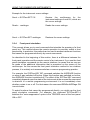
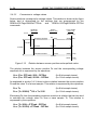
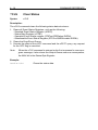
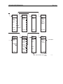
3.4 Acquisition
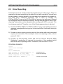
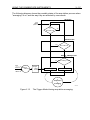
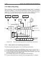
3.4.1
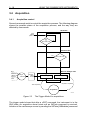
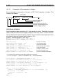
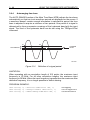
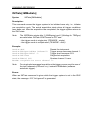
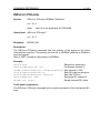
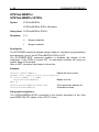
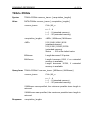
Acquisition control
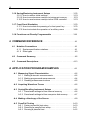
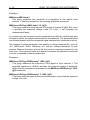
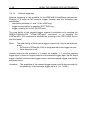
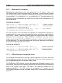
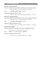
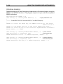
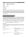
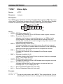
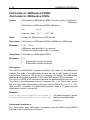
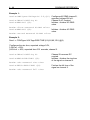
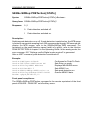
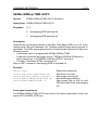
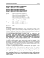
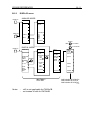
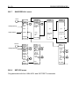
Several commands exist to control the acquisition process. The following diagram
shows the possible states of the acquisition process, and the way they are
affected by commands.
IDLE state
*RST
ABORt
power on
INIT
or
INIT:CONT ON
No
Yes
INITiated state
No
Yes
INIT:CONT ON
Wait for TRIGger state
BUS
IMMediate
INTernal
TRIGger
:SOURce
TRIGger
:LEVel
:SLOPe
Wait for trigger
Wait for complete
LINE
Acquisition completed
Start acquisition
Acquisition
ST7186
Figure 3.3
The Trigger Model for acquisitions
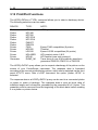
The trigger model shows that after a *RST command, the instrument is in the
IDLE state. An acquisition doesn’t start until an INITiate command is received.
Initiation of the oscilloscope occurs by sending the INITiate[:IMMediate] command
USING THE COMBISCOPE INSTRUMENTS
3 - 19
or by setting INITiate:CONTinuous to ON. The INITiate[:IMMediate] command
causes the CombiScope instrument to perform one complete acquisition cycle.
Upon completion of the cycle the instrument returns to the IDLE state.
The INItiate:CONTinuous command is used to select whether the instrument is
continuously initiated or not. When INItiate:CONTinuous is set to ON, the
instrument immediately exits IDLE and starts an acquisition cycle. On completion
of each cycle, the instrument does not return to the IDLE state, but immediately
starts another acquisition cycle.
Before the acquisition takes place, the trigger conditions must be satisfied. These
conditions are programmable to suit the needs of your application, as described in
the next section. After a *RST command, there are no trigger conditions to be met.
So, an INITiate command causes the CombiScope instrument to immediately
trigger the acquisition.
Executing the measurement instructions MEASure? and READ? causes the
acquisition to become initiated automatically. No separate INITiate commands are
needed. When the FETCh? instruction is used, the instrument must have been
initiated either by a preceding INITiate[:IMMediate] command, or implicitly by a
READ? or MEASure? instruction.
When the CombiScope instrument receives the ABORt command, any
acquisition that is in progress is aborted immediately, and the instrument returns
to the IDLE state. The same occurs when *RST is received. The ABORt
command distinguishes from *RST in that *RST also resets the instrument
settings, whereas, ABORt does not. For example, when INITiate:CONTinuous is
set to ON, a *RST command not only aborts the pending acquisition and forces
the instrument to the IDLE state, but it also sets INITiate:CONTinuous to OFF,
preventing the acquisition to initiate again. Since ABORt does not affect the
instrument settings, an aborted acquisition cycle is immediately initiated again.
When the instrument is in the IDLE state, the "no-pending operation" flag that is
associated with the acquisition is set True. The *OPC and *OPC? commands use
this flag to signal their "Operation Completed" response. Notice that if
INITiate:CONTinuous is set to ON, the instrument does not return to the IDLE
state when an acquisition cycle has completed. This means that no "Operation
Completed" response is generated after the *OPC and *OPC? commands.
3 - 20
3.4.1.1
USING THE COMBISCOPE INSTRUMENTS
Triggering
After the measurement is initiated, the CombiScope instrument starts the real
acquisition when the trigger conditions are satisfied, e.g., when the selected
trigger event occurs. The trigger conditions can be ignored during a specific holdoff time, which can be programmed using the TRIGger:HOLDoff command.
During the hold-off time the event detector is inhibited from acting on any trigger.
Trigger Type
The TRIGger:TYPE command selects the type of triggering, which can be
programmed to EDGE triggering (normal trigger mode), VIDeo triggering (refer to
section 3.4.1.2 "Video triggering"), LOGic, or GLITch triggering. After a *RST
command, the trigger type is EDGE.
Note:
Logic state, pattern, or glitch settings cannot be programmed using SCPI
commands.
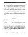
Trigger Source
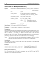
The TRIGger:SOURce command selects the source for the trigger event. The
receipt of the GPIB interface message GET (Group Execute Trigger) or the
common command *TRG serves as the trigger event when BUS is selected as
trigger source.
The trigger event is determined by the AC line voltage when LINE is selected, and
is derived from the input signal when INTernal is programmed as trigger source.
For the 2-channel CombiScope instruments, EXTernal can be programmed as the
trigger source. In that case, channel 4 is selected as external trigger input.
A numeric suffix is used to specify the channel number. For example,
TRIGger:SOURce INT2 selects the signal at input channel 2 to trigger the
acquisition.
When IMMediate is selected, an acquisition does not wait for a trigger event. So,
an INITiate command causes the acquisition to begin immediately. After a *RST
command, the trigger source is IMMediate, which means no trigger is required.
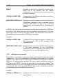
Trigger Level
The TRIGger:LEVel command allows you to set the trigger level for all input
channels. Programming the trigger level automatically switches off level peakpeak. The trigger level can be programmed only when the TRIGger:SOURce is
INTernal. The TRIGger:LEVel:AUTO command allows you to switch level peakpeak on or off. Switching on level peak-peak, deactivates the trigger level. After a
*RST command the TRIGger:LEVel is set to its maximum value and level peakpeak is switched off.
USING THE COMBISCOPE INSTRUMENTS
3 - 21
Trigger Slope
The TRIGger:SLOPe command allows you to define the trigger edge for all input
channels, which can be POSitive, NEGative, or EITHer. After a *RST command
the TRIGger:SLOPe is set to POSitive.
PROGRAM EXAMPLE:
CALL Send(0, 8, "CONFigure:PTPeak (@2)", 1)
’Configures channel 2
CALL Send(0, 8, "SENSe:FUNCtion 'XTIMe:VOLTage2'", 1) ’Sets channel 2 ON
CALL Send(0, 8, "TRIGger:SOURce INTernal2", 1)
’Trigger source = channel 2
CALL Send(0, 8, "TRIGger:LEVel 0.2", 1)
’Trigger level = 0.2 V
'The TRIGger:LEVel command also switches level peak-peak off.
CALL Send(0, 8, "TRIGger:SLOPe NEGative", 1)
’Trigger slope = negative
CALL Send(0, 8, "INITiate", 1)
’Single initiation
CALL Send(0, 8, "FETCh:PTPeak? (@2)", 1)
’Queries for peak-to-peak
response$ = "
"
CALL Receive(0, 8, response$, 256)
’Enters peak-to-peak
PRINT "Measured peak-to-peak = "; response$
’Prints peak-to-peak
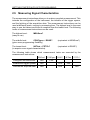
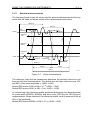
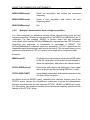
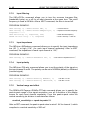
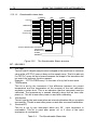
Trigger Coupling
The TRIGger:LPASs and TRIGger:HPASs commands allow you to select the
Main Time Base (MTB) trigger coupling by programming a fixed cutoff frequency.
The possible trigger coupling options AC coupling, DC coupling, Low Frequency
reject, and High Frequency reject are mutually exclusive. The TRIGger:LPASs
and TRIGger:HPASs commands are also mutually exclusive. So, activating the
Low-Pass filter will switch off the High-Pass filter, and vice versa. After a *RST
command, the cutoff frequency is 10 Hertz, which selects trigger coupling AC.
Note:
When the trigger source is INTernal<n>, signal coupling for one input
channel (n) can be programmed to AC, DC, or GROund using the
INPut<n>:COUPling command.
3 - 22
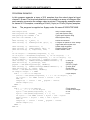
USING THE COMBISCOPE INSTRUMENTS
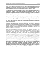
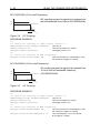
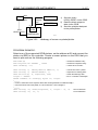
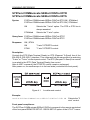
DC COUPLING (0 Hz cutoff frequency):
DC coupling causes the signal to be passed over
the full bandwidth (from 0 Hz to 60/100/200 MHz).
0dB
-3dB
DC COUPLING
DC
FULL BANDWIDTH
FREQ.
ST7427
Figure 3.4
DC Coupling
PROGRAM EXAMPLE:
***
*** Select DC coupling on input signal channel 2.
SENSe:FUNCtion:ON "XTIMe:VOLTage2"
Sets CH2 on.
INPut2:COUPling DC
Sets CH2 input signal DC coupled.
TRIGger:SOURce INTernal2
Sets trigger source = CH2.
***
*** Select DC coupling on MTB triggering.
TRIGger:FILTer:LPASs:STATe ON
Sets Low-Pass filter on + cutoff frequency = 0 Hz;
this selects MTB trigger DC coupling.
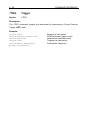
AC COUPLING (10 Hz cutoff frequency):
0dB
-3dB
AC COUPLING
10Hz
AC coupling causes the signal to be passed from
10 Hz to the full bandwidth frequency
(60/100/200 MHz).
FULL BANDWIDTH
FREQ.
ST7426
Figure 3.5
AC Coupling
PROGRAM EXAMPLE:
***
*** Select AC coupling on input signal channel 3.
SENSe:FUNCtion:ON "XTIMe:VOLTage3"
Sets CH3 on.
INPut3:COUPling AC
Sets CH3 input signal AC coupled.
TRIGger:SOURce INTernal3
Sets trigger source = CH3.
***
*** Select AC coupling on MTB triggering.
TRIGger:FILTer:LPASs:STATe ON
Sets Low-Pass filter on + cutoff frequency = 0 Hz;
this selects MTB trigger DC coupling.
TRIGger:FILTer:LPASs:FREQuency 10
Sets cutoff frequency = 10 Hz; this selects
MTB trigger AC coupling.
USING THE COMBISCOPE INSTRUMENTS
3 - 23
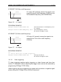
LF-REJECT (30 KHz cutoff frequency):
LF reject (HF passed) causes the signal to be
passed from the cutoff frequency (30 KHz) to the
full bandwidth frequency (60/100/200 MHz).
LF -REJECT
0dB
-3dB
30kHz
FULL BANDWIDTH
FREQ.
ST7428
Figure 3.6
LF Reject
PROGRAM EXAMPLE:
TRIGger:FILTer:LPASs:STATe ON
TRIGger:FILTer:LPASs:FREQuency 3E+4
Sets Low-Pass filter on + cutoff frequency = 0 Hz
(DC coupling).
Sets cutoff frequency = 30 KHz;
this selects MTB trigger LF-reject.
HF-REJECT (30 KHz cutoff frequency)
HF reject (LF passed) causes the signal to be
passed from 0 Hz to the cutoff frequency
(30 KHz).
HF-REJECT
0dB
-3dB
30kHz
FULL BANDWIDTH
FREQ.
ST7429
Figure 3.7
HF Reject
PROGRAM EXAMPLE:
***
*** Select HF-reject on MTB triggering.
TRIGger:FILTer:HPASs:STATe ON
Sets High-Pass filter on;
this selects MTB trigger HF-reject.
3.4.1.2
Video triggering
TV video triggering enables stable triggering on video frames and lines from
various TV standards without adjusting the trigger level, and can be selected by
programming TRIGger:TYPE VIDeo.
Video triggering can be programmed on signals with a positive or negative signal
polarity using the TRIGger:VIDeo:SSIGnal command.
3 - 24
USING THE COMBISCOPE INSTRUMENTS
The video trigger mode can be programmed to field1, field2, or lines using the
TRIGger:VIDeo:FIELd... commands. The video trigger line can be programmed
using the TRIGger:VIDeo:LINE command.
The video system can be selected using the TRIGger:VIDeo:FORMat:...
commands. The following standard video systems are supported:
- NTSC
: 525 lines per frame
- PAL
: 625 lines per frame
- SECAM : 625 lines per frame
- HDTV
: 1050/1125/1250 lines per frame
1) Select video triggering and video standard.
Examples: TRIGger:TYPE VIDeo
Selects TV video triggering.
TRIGger:VIDeo:FORMat:TYPE SECAM
Selects the SECAM standard with 625 lines per frame.
TRIGger:VIDeo:FORMat:LPFRame 1125
Selects the HDTV standard with 1125 lines per frame.
2) Select video "lines" triggering and program the line to trigger on.
Examples: TRIGger:VIDeo:FIELd:SELect ALL
Selects the video lines trigger mode.
TRIGger:VIDeo:LINE 512
Selects video line number 512.
3) Select video "field1/2" triggering and program the line to trigger on.
Examples: TRIGger:VIDeo:FIELd:SELect NUMBer
Selects video field triggering.
TRIGger:VIDeo:FIELd:NUMBer 2
Selects the video field2 trigger mode.
TRIGger:VIDeo:FORMat:TYPE PAL
Selects the PAL standard with 625 lines per frame.
TRIGger:VIDeo:LINE 123
Selects video line number 123. As a result the video mode is
automatically switched to field1 (field1 = lines 1 .. 312).
TRIGger:VIDeo:LINE 325
Selects video line number 325. As a result the video mode is
automatically switched to field2 (field2 = lines 313 .. 625).
TRIGger:VIDeo:FIELd:NUMBer 1
Selects the video field1 trigger mode. As a result the video
line number is automatically switched to 13 (= 325 - 625/2).
USING THE COMBISCOPE INSTRUMENTS
3.4.1.3
3 - 25
The trigger modes
A combination of the INITiate:CONTinuous and TRIGger:SOURce command
allows you to define the following trigger modes:
INITiate
:CONTinuous
TRIGger
:SOURce
>>>Single-shot<<<
Generates one sweep, regardless of any
trigger settings (valid after *RST).
OFF
IMMediate
>>>Single-shot<<<
Generates one sweep, triggered using
trigger settings.
OFF
INTernal<n>
or
LINE
Trigger mode:
>>> Single-shot <<<
Generates one sweep, externally triggered OFF
via channel 4 (only for PM33x0B).
EXTernal
>>>Auto trig<<<
Generates continuous sweeps,
independent of any trigger settings.
ON
IMMediate
>>>Normal trig<<<
Generates continuous sweeps, triggered
using trigger settings.
ON
INTernal<n>
or
LINE
>>> Normal trig <<<
Generates continuous sweeps, externally
ON
triggered via channel 4 (only for PM33x0B).
>>>Single-Shot<<<
Generates one sweep triggered by *TRG
or GET, regardless of any trigger settings.
Table 3.1
ON
or
OFF
The TRIGger modes
EXTernal
BUS
3 - 26
USING THE COMBISCOPE INSTRUMENTS
Only in the single-shot and multiple-shot trigger mode (INITiate:CONTinuous
OFF), the bits 3 (SWEeping) and 5 (Waiting for TRIGger) in the OPERation status
are valid. Also the Operation Complete bit (OPC bit 0) in the standard Event
Status Register (ESR) is valid. This allows you to detect whether the instrument
is armed (initiated), triggered (busy with acquisition), or finished with the last
acquisition, i.e., ready for the next acquisition.
SINGLE-SHOT MODE (TB MODE - single):
Commands:
CONFigure:AC
Configures instrument and sets
single-shot mode.
OPERATION STATUS BITS:
bit 5
Wait for TRIG
bit 3
SWEeping
OPC
idle state (after *RST)
0
0
0
Wait for trigger state (INIT received)
Wait for complete (triggered)
1
1
0
0
0
0
= armed
or busy
Finished with acquisition
0
0
1
= ready
STATE DESCRIPTION:
MULTIPLE-SHOT MODE (TB MODE - multi):
OPERATION STATUS BITS:
bit 5
Wait for TRIG
bit 3
SWEeping
OPC
idle state (after *RST)
0
0
0
Wait for trigger state (INIT received)
1
0
0
= armed
Wait for complete (triggered)
0
1
0
= busy
Finished with acquisition
0
0
1
= ready
STATE DESCRIPTION:
The bits 3 (SWEeping) and 5 (Waiting for TRIGger) also reflect the acquisition
status, when the "SINGLE ARM'D" button on the front panel was pressed.
Commands:
SYSTem:KEY 101
DISPlay:MENU TBMode
SYSTem:KEY 1
Performs AutoSet.
Displays TBMODE menu.
Sets INIT:CONT OFF and sets
multiple-shot mode.
USING THE COMBISCOPE INSTRUMENTS
3.4.1.4
3 - 27
Pre- and post-triggering
When pre-triggering is selected, the real trace acquisition begins before the
moment that the trigger occurs. Triggering occurs when the trigger conditions are
satisfied and the instrument leaves the "Wait for TRIGger" state as shown in the
trigger diagram of figure 3.3. In a similar way, post-triggering causes the
acquisition to begin after the moment that the trigger occurs.
trigger moment
SENSe:SWEep:OFFSet:TIME
pre trigger
Trace
time axis
end
begin
total acquisition time
SENSe:SWEep:TIME
trigger moment
Figure 3.8
ST7190
Pre-triggering
SENSe:SWEep:OFFSet:TIME
post trigger
Trace
total acquisition time
SENSe:SWEep:TIME
Figure 3.9
time axis
end
begin
ST7191
Post-triggering
Pre- and post-triggering are programmed with the SENSe:SWEep:OFFSet:TIME
command. A positive parameter value specifies a post-trigger delay, whereas, a
negative value results in a pre-trigger view.
After *RST, the SENSe:SWEep:OFFSet:TIME is set to -0.005, which results in a
pre-trigger view of 5 ms. Because the *RST value of the total acquisition time
(SENSe:SWEep:TIME) is 10 ms, the trigger point is positioned in the middle of
the trace.
PROGRAM EXAMPLE:
CALL Send(0, 8, "SENSe:SWEep:OFFSet:TIME 0.001", 1)
CALL Send(0, 8, "SENSe:SWEep:OFFSet:TIME -1E-3", 1)
’1 ms post-trigger
’1 ms pre-trigger
3 - 28
3.4.1.5
USING THE COMBISCOPE INSTRUMENTS
External triggering
External triggering is only possible for the PM33x0B CombiScope instruments.
Channel 4 is used as the external trigger channel with the following view
possibilities:
- attenuator positions 0.1 and 1 V/div (AMP key).
- trigger slope positive or negative (EXT TRIG key).
- trigger coupling AC or DC (AC/DC key).
The view facility of the external trigger channel is switched on by sending the
SENSe:FUNCtion:ON "XTIMe:VOLTage4" command, or by sending the
SYSTem:KEY 812 command to simulate the pressing of the TRIG VIEW key on
the front panel.
Note:
The view facility of the external trigger channel can only be switched on
when:
• EXTernal or INTernal4 (CH4) is programmed as the trigger source.
• Peak detection is off.
Autoset scans for the presence of a signal on channel 1, 2, and the external
trigger input. If there is a signal present on the external trigger input, the EXTernal
trigger channel is selected as trigger source, and the external trigger view facility
becomes active.
Limitation: The amplitude of the external trigger signal must be high enough for
the sensitivity of the external trigger input (0.1 or 1 V/div.).
USING THE COMBISCOPE INSTRUMENTS
3.4.2
3 - 29
Reading trace acquisitions
Once acquisitions are completed, the resulting traces ares placed in TRACe
memory, as shown in the following figure.
INPut
TRACe
SENSe
memory
@1
INPut[1]
:VOLTage[1]
CH 1
@2
INPut2
:VOLTage2
CH 2
:SWEep
@3
INPut3
:VOLTage3
CH 3
@4
INPut4
:VOLTage4
CH 4
Main Time Base
ST7160
Figure 3.10
The trace acquisition flow
The last acquired trace at input channel 1 is placed in the TRACe memory
element named CH1. The trace acquired at channel 2 in CH2, etc. This trace data
can be read by using the TRACe[:DATA]? query.
Example:
TRACe? CH2
Returns the trace that was last acquired at input channel 2.
When new acquisitions are executed, the previously stored traces are not
automatically saved, but overwritten by the new result. When these traces need
to be saved, they have to be copied into other TRACe memory elements, before
a new acquisition is initiated. Refer to section 3.10.2 "Copying traces to memory"
for a description about how to copy traces.
As response to the TRACe? query the data is returned as block data.
Section 3.4.3 "Conversion of trace data" specifies the coding of this data and
describes how to convert this data into voltage values.
3 - 30
3.4.2.1
USING THE COMBISCOPE INSTRUMENTS
Single-shot acquisition
PROGRAM EXAMPLE:
In this example a single-shot trace acquisition is done via channel 1. The trace
bytes are entered as characters in the string response$.
DIM response AS STRING * 1033
CALL Send(0, 8, "*RST", 1)
’Dimensions trace buffer
’Resets the instrument
’Trigger source becomes IMMediate
’Number of trace samples becomes 512
’Number of trace sample bits becomes 16
’Configures for optimal AC-RMS settings
’Initiates single acquisition
’Requests for channel 1 trace data
CALL Send(0, 8, "CONFigure:AC", 1)
CALL Send(0, 8, "INITiate", 1)
CALL Send(0, 8, "*WAI;TRACe? CH1", 1)
’
’Notice the *WAI; before TRACe?. The *WAI command takes care that the
’TRACe? CH1 command is executed when the INITiate command is finished.
’
CALL Receive(0, 8, response$, 256)
’Reads the channel 1 trace data
3.4.2.2
Repetitive acquisitions
PROGRAM EXAMPLE:
In this example 10 trace acquisitions are done via channel 1. The trace bytes are
entered as characters in the string response$. The 10 trace buffers are written to
the file TRACE10 on the hard disk. Triggering is done via the GPIB by sending the
*TRG command.
’Dimensions trace buffer
’Resets the instrument
’Trigger source becomes IMMediate
’Number of trace samples becomes 512
’Number of trace sample bits becomes 16
CALL Send(0, 8, "CONFigure:AC (@1)", 1) ’Configures for optimal AC-RMS settings.
CALL Send(0, 8, "TRIGger:SOURce BUS", 1) ’Trigger source = GPIB
OPEN "O",#1,"TRACE10"
’Opens file TRACE10
FOR i=1 TO 10
’10 sequential trace acquisitions
CALL Send(0, 8, "INITiate", 1)
’Initiates an acquisition
CALL Send(0, 8, "*TRG", 1)
’Triggers via the GPIB
CALL Send(0, 8, "*WAI;TRACe? CH1", 1) ’Requests for channel 1 trace
’
’Notice the *WAI; before TRACe?. The *WAI command takes care that
’the TRACe? CH1 command is executed when the INITiate command is finished.
’
CALL Receive(0, 8, response$, 256)
’Reads the channel 1 trace
PRINT #1, response$
’Writes the trace buffer to file
NEXT i
’Next trace acquisition
CLOSE
’Closes file TRACE10
DIM response AS STRING * 1033
CALL Send(0, 8, "*RST", 1)
USING THE COMBISCOPE INSTRUMENTS
3.4.3
3 - 31
Conversion of trace data
The trace data is sent as a block of binary codes. Trace samples can be formatted
to consist of 8 bits (1 byte) or 16 bits (2 bytes) codes, which can be selected by
the FORMat command. Refer to section 3.10.1 "Trace formatting" for a further
explanation of this command. After *RST the samples are sent as 2 byte codes.
When samples are formatted as two bytes, the most significant byte (msb) is sent
first, followed by the least significant byte (lsb). The sample values that are sent
in the block, are coded according to the two’s complement notation. The relation
between the screen positions, the values of the trace samples and the decimal
value of the corresponding binary codes, is shown in the figure below.
Screen
position (Ps)
top
Trace sample
value (Ts)
32767 (127)
32767 (127)
25600 (100)
25600 (100)
1 (1)
0 (0)
screen mid
range
Decimal value
of byte code
-1 (-1)
1 (1)
0 (0)
65535 (255)
-25600 (-100)
39936 (156)
-32768 (-128)
32768 (128)
trace
range
bottom
ST7187
Note: Numbers between parenthesis apply to single byte format.
Figure 3.11
Relation between screen position and trace value
The value of the trace points relate to the vertical position of the corresponding
sample on the screen of the CombiScope instrument. As the figure above shows,
the sample with value 25600 corresponds with the top position of the screen.
Similarly, the samples with values -25600 and 0 correspond to the bottom and
mid-position respectively. This applies to trace samples that are formatted to
consist of 16 bits (2 bytes). The values that apply to the 8 bit (1 byte) format are
placed between parenthesis.
The ADC allows trace acquisitions that are somewhat outside the vertical screen
boundaries. Trace acquisitions use the full dynamic range of the ADC. This results
in a dynamic trace range of 65535 points, whereas the screen range is limited to
51200 points.
3 - 32
3.4.3.1
USING THE COMBISCOPE INSTRUMENTS
Conversion of 8-bit samples to integer
As an example a conversion of a trace of 512 "8-bit" samples is shown. The
format is as follows:
trace bytes
# 3 5 1 4 <8> <byte 1> . . . <byte 512> <checksum> <NL>
trace sample 512
trace sample 1
byte with decimal value 8
number of trace bytes (514)
number of digits of 514
PROGRAM EXAMPLE:
In this example a trace acquisition of 1 byte samples is done. Thereafter, the trace
data is read and converted to integer samples in the array "trace", and the number
of trace bytes and trace samples is printed. The conversion from single byte value
to integer is done as follows (refer to figure 3.12):
If byte ≥ 128 then integer = byte - 256.
Example: byte = 255 --> integer = 255 - 256 = -1.
DIM trace(512)
’Array of 512 integers
DIM response AS STRING * 520
’Trace response buffer
CALL Send(0, 8, "*RST", 1)
’Resets the instrument
CALL Send(0, 8, "FORMat INTeger,8", 1)
’Data format of 8-bits samples
CALL Send(0, 8, "INITiate", 1)
’Single shot initiation
CALL Send(0, 8, "*WAI;TRACe? CH1", 1)
’Queries for channel 1 trace
CALL Receive(0, 8, response$, 256)
’Reads the channel 1 trace
PRINT "Number of read bytes ="; IBCNT%
’IBCNT% = number of read bytes
’
’The contents of the response$ string of this example will be as follows:
’ # 3 5 1 4 <8> <byte 1> ... <byte 512> <checksum> <10> ’<10> is terminating LF
’
nr.of.digits = VAL(MID$(response$, 2, 1))
nr.of.bytes = VAL(MID$(response$, 3, nr.of.digits)) - 2
PRINT "Number of trace bytes ="; nr.of.bytes
sample.length = ASC(MID$(response$, 3 + nr.of.digits, 1))
nr.of.samples = nr.of.bytes / (sample.length / 8)
PRINT "Number of trace samples ="; nr.of.samples
FOR i = 1 TO nr.of.samples
trace(i) = ASC(MID$(response$, i + 3 + nr.of.digits, 1))
IF trace(i) > 127 THEN
trace(i) = trace(i) - 256
END IF
NEXT i
USING THE COMBISCOPE INSTRUMENTS
3.4.3.2
3 - 33
Conversion of 16-bit samples to integer
As an example a conversion of a trace of 512 "16-bit" samples is shown. The
format is as follows:
trace bytes
# 4 1 0 2 6 <16> <msb 1> <lsb 1> . . . <msb 512> <lsb 512> <checksum> <NL>
trace sample 512
trace sample 1
byte with decimal value 16
number of trace bytes (1026)
number of digits of 1026
PROGRAM EXAMPLE:
In this example a trace acquisition of 2 byte samples is done. Thereafter, the trace
data is read and converted to integer samples in the array "trace", and the number
of trace bytes samples is printed. The conversion from double byte (byte1 = msb
and byte2 = lsb) to integer is done as follows (refer to figure 3.12):
If byte1 < 128 then integer = byte1 * 256 + byte2.
If byte1 ≥ 128 then integer = (byte1 - 256) * 256 + byte2.
Example: byte1 = 255 & byte2 = 32 --> integer = (255 - 256) * 256 + 32 = - 224.
DIM trace(512)
DIM response AS STRING * 1033
CALL Send(0, 8, "*RST", 1)
’Array of 512 integers
’Trace response buffer
’Resets the instrument
’Sets 16 bit sample data format
’Single shot initiation
’Queries for channel 1 trace
’Reads the channel 1 trace
’IBCNT% = length of trace buffer
CALL Send(0, 8, "INITiate", 1)
CALL Send(0, 8, "*WAI;TRACe? CH1", 1)
CALL Receive(0, 8, response$, 256)
PRINT "Number of trace bytes ="; IBCNT%
’
’The contents of the response$ string of this example will be as follows:
’# 4 1 0 2 6 <16> <msb1> <lsb1> ... <msb512> <lsb512> <sum> <10>
’
nr.of.digits = VAL(MID$(response$, 2, 1))
nr.of.bytes = VAL(MID$(response$, 3, nr.of.digits)) - 2
PRINT "Number of trace bytes ="; nr.of.bytes
sample.length = ASC(MID$(response$, 3 + nr.of.digits, 1))
nr.of.samples = nr.of.bytes / (sample.length / 8)
PRINT "Number of trace samples ="; nr.of.samples
FOR i = 1 TO nr.of.samples
J = 2 * i + 2 + nr.of.digits
’Pointer to next sample
byte1 = ASC(MID$(response$, J, 1))
’Most Significant Byte
byte2 = ASC(MID$(response$, J + 1, 1)) ’Least Significant Byte
IF byte1 < 128 THEN
trace(i) = byte1 * 256 + byte2
ELSE trace(i) = (byte1 - 256) * 256 + byte2
END IF
NEXT i
3 - 34
3.4.3.3
USING THE COMBISCOPE INSTRUMENTS
Conversion to voltage values
Screen positions correspond to voltage values. This relation is shown in the figure
below, and is determined by the settings that are programmed by the
SENSe:VOLTage:RANGe:PTPeak
and
SENSe:VOLTage:RANGe:OFFSet
commands.
Amplitude
value (Vs)
Screen
position (Ps)
0 Volt
Trace sample
value (Ts)
32767 (127)
-OFFSet+PTPeak/2
top 100%
-OFFSet
mid 0%
25600 (100)
OFFSet
PTPeak
-OFFSet-PTPeak/2
-100%
bottom
0 (0)
-25600 (-100)
-32768 (-128)
ST7188
Figure 3.12
Relation between screen position and amplitude value
The relation between the screen position Ps and the corresponding voltage
amplitude Vs is expressed by the equations:
Vs = (Ps * PTPeak) / 200 - OFFSet
Vs = (Ps * PTPeak) / 51200 - OFFSet
(for 8-bit sample traces)
(for 16-bit sample traces)
As explained in section 3.4.3, there is also a relation between the screen position
Ps and the value Ts of a trace sample. This relation is expressed by the equations:
Ps = Ts
Ps = (Ts / 25600) * 100 = Ts / 256
(for 8-bit sample traces)
(for 16-bit sample traces)
Eliminating Ps from the preceding equations results in a relation that can be used
to calculate the voltage value Vs from a trace sample Ts. This relation is
expressed by the equations:
Vs = (Ts / 200) * PTPeak - OFFSet
Vs = (Ts / 51200) * PTPeak - OFFSet
(for 8-bit sample traces)
(for 16-bit sample traces)
USING THE COMBISCOPE INSTRUMENTS
3 - 35
PROGRAM EXAMPLE:
In this program example a trace of 512 samples from the actual signal at input
channel 1 is read. The received data block is converted to an array of voltages. After
each sample conversion the voltage value is printed. This program example works
for traces of 512 samples, consisting of 8 bits (1 byte) or 16 bits (2 bytes) samples.
Note:
The program is supplied on floppy under file name EXCNVTRC.BAS.
DIM sample(512)
DIM response AS STRING * 1033
DIM peaktop AS STRING * 10
DIM offs AS STRING * 10
’
CALL Send(0, 8, "*RST", 1)
CALL Send(0, 8, "CONFigure:AC (@1)", 1)
’Array of sample voltages
’Trace data response string
’Peak-to-peak response string
’Offset response string
’Resets the instrument
’Configures for optimal AC-RMS settings
’Signal-offset also becomes zero
’Initiates single acquisition
’Requests channel 1 trace
’Reads channel 1 trace
CALL Send(0, 8, "INITiate", 1)
CALL Send(0, 8, "*WAI;TRACe? CH1", 1)
CALL Receive(0, 8, response$, 256)
’
nr.of.digits = VAL(MID$(response$, 2, 1))
nr.of.bytes = VAL(MID$(response$, 3, nr.of.digits)) - 2
sample.length = ASC(MID$(response$, 3 + nr.of.digits, 1))
nr.of.samples = nr.of.bytes / (sample.length / 8)
CALL Send(0, 8, "SENSe:VOLTage:RANGe:PTPeak?", 1)
’Queries ptp
CALL Receive(0, 8, peaktop$, 256)
’Reads ptp
ptpeak = VAL(LEFT$(peaktop$, IBCNT%))
’IBCNT% = length
CALL Send(0, 8, "SENSe:VOLTage:RANGe:OFFSet?", 1)
’Queries offset
CALL Receive(0, 8, offs$, 256)
’Reads offset
offset = VAL(LEFT$(offs$, IBCNT%))
’IBCNT% = length
IF sample.length = 1 THEN
FOR i = 1 TO nr.of.samples
’1-byte samples
trace% = ASC(MID$(response$, i + 3 + nr.of.digits, 1))
IF trace% > 127 THEN trace% = trace% - 256
END IF
sample(i) = trace% / 200 * ptpeak - offset
PRINT sample(i);
NEXT i
ELSE
FOR i = 1 TO nr.of.samples
’2-byte samples
J = 2 * i + 2 + nr.of.digits
’Pointer to next sample
byte1 = ASC(MID$(response$, J, 1))
’M.S.B.
byte2 = ASC(MID$(response$, J + 1, 1))
’L.S.B.
IF byte1 < 128 THEN trace% = byte1 * 256 + byte2
ELSE trace% = (byte1 - 256) * 256 + byte2
END IF
sample(i) = trace% / 51200 * ptpeak - offset
PRINT sample(i);
NEXT i
END IF
3 - 36
USING THE COMBISCOPE INSTRUMENTS
3.5 Averaging Acquisition Data
Acquired traces and measured signal characteristics can be averaged over a
number of acquisitions. The preprocessing AVERAGE function of the
CombiScopes instruments can be enabled by using the SENSe:AVERage[STATe]
command. When this function is set to ON, averaging is done according to the
following formula:
AVG n =
∑ ( X1 + .. + Xn ) ⁄ n
In the expression, n specifies the number of acquisitions that is averaged. This
parameter can be programmed by using the SENSe:AVERage:COUNt
command. X represents the acquisition result to be averaged.
Example:
Send → SENSe:AVERage:COUnt 16
Send → SENSe:AVERage ON
’ This sets the average count factor at
16, which means 16 sequential
acquisitions are averaged.
’ This enables the AVERAGE function.
When SENSe:AVERage is set to ON and an acquisition is initiated, the
CombiScope instrument takes n (SENSe:AVERage:COUNt) successive
acquisitions, as shown in the figure on the next page. When sufficient acquisitions
are taken, the final averaged result is returned. Intermediate results cannot be
queried.
PROGRAM EXAMPLE:
Acquire the trace of the actual signal on channel 1 and measure the amplitude
and frequency (averaged over 4 acquisitions).
DIM trace AS STRING * 1033
’Dimensions trace string
DIM amplitude AS STRING * 10
’Dimensions amplitude string
DIM frequency AS STRING * 10
’Dimensions frequency string
CALL Send(0, 8, "CONFigure:AC (@1)", 1)
’Configures for AC-RMS
CALL Send(0, 8, "SENSe:AVERage:COUNt 4", 1) ’Average factor = 4
CALL Send(0, 8, "SENSe:AVERage ON", 1)
’Averaging is turned on
CALL Send(0, 8, "INITiate", 1)
’Initiates the averaging acquisition
CALL Send(0, 8, "*WAI;TRACe? CH1", 1)
’Queries for channel 1 trace
CALL Receive(0, 8, trace$, 256)
’Enters channel 1 trace
’The trace samples are averaged over 4 sequential trace acquisitions.
CALL Send(0, 8, "READ:AMPLitude?", 1)
’Reads the amplitude
CALL Receive(0, 8, amplitude$, 256)
’Enters the amplitude
CALL Send(0, 8, "FETCh:FREQuency?", 1)
’Fetches the frequency
CALL Receive(0, 8, frequency$, 256)
’Enters the frequency
’The amplitude and frequency are averaged over 4 sequential measured values.
USING THE COMBISCOPE INSTRUMENTS
3 - 37
The following diagram shows the possible states of the acquisition process when
"averaging" is on, and the way they are affected by commands.
IDLE state
*RST
ABORt
power on
INIT
or
INIT:CONT ON
No
Yes
INITiated state
No
Yes
INIT:CONT ON
Wait for AVERage state
Yes
No
SENSe:AVERage:COUNt
LINE
TRIGger
:SOURce
INTernal
IMMediate
TRIGger
:LEVel
:SLOPe
Wait for trigger
Wait for complete
1
acquisition
+
averaging
ST7189
Figure 3.13
The Trigger Model during acquisition averaging
3 - 38
USING THE COMBISCOPE INSTRUMENTS
3.6 Channel Selection
Input channels can be switched on or off by using the SENSe:FUNCtion[:ON] or
SENSe:FUNCtion:OFF commands. An input channel is selected by specifying
the parameter "XTIMe:VOLTage<n>", where the numeric suffix <n> specifies the
input channel number. After a *RST command, channel 1 is turned on and the
other channels off (including the EXTernal input for PM33x0A).
Addition of two channels can be selected by specifying the "XTIMe:VOLTage:SUM"
parameter as follows:
> Addition of CH1 and CH2:
"XTIMe:VOLTage:SUM 1,2"
> Addition of CH3 and CH4:
"XTIMe:VOLTage:SUM 3,4"
Note:
Enabling of the addition of input channels (e.g. CH3+CH4), automatically
switches channel 3 and channel 4 on. Disabling of the addition of two
channels (e.g. CH3+CH4), automatically switches channel 3 and
channel 4 off, provided at least one channel remains on.
Programming tip:
If CH1+CH2 is on and CH3 and CH4 are off, CH1+CH2 cannot be programmed
off by sending: SENSE:FUNCtion:OFF "XTIME:VOLTage:SUM 1,2"
Instead, send the command:
SENSe:FUNCtion:ON "XTIME:VOLTage2"
’Sets CH2 on
INPut
SENSe
TRACe
:FUNCtion
memory
:OFF
@1
INPut[1]
:VOLTage[1]
"XTIMe:VOLTage1"
CH 1
[:ON]
:OFF
@2
INPut2
:VOLTage2
"XTIMe:VOLTage2"
CH 2
[:ON]
:SWEep
:OFF
@3
INPut3
:VOLTage3
"XTIMe:VOLTage3"
CH 3
[:ON]
:OFF
@4
INPut4
:VOLTage4
"XTIMe:VOLTage4"
CH 4
[:ON]
Main Time Base
ST7158
Figure 3.14
Input channel control
PROGRAM EXAMPLE:
CALL Send(0, 8, "SENSe:FUNCtion 'XTIMe:VOLTage:SUM 1,2'", 1)
’Sets CH1+CH2 on
CALL Send(0, 8, "SENSe:FUNCtion:ON ’XTIMe:VOLTage2’", 1)’
’Sets CH2 on, CH1+CH2 off, CH1 remains off.
USING THE COMBISCOPE INSTRUMENTS
3 - 39
3.7 Signal Conditioning
The INPut subsystem allows you to condition the input signals, such as
AC/DC/GROund coupling, input filtering, and input impedance selection.
In the digital mode, the SENSe:VOLTage<n>:RANGe:AUTO command allows
you to enable autoranging of the attenuation for each of the input channels <n>
separately.
SENSe
INPut
:FUNCtion
:OFF
@1
INPut[1]
:VOLTage[1]
"XTIMe:VOLTage1"
[:ON]
:OFF
@2
INPut2
:VOLTage2
"XTIMe:VOLTage2"
[:ON]
:SWEep
:OFF
@3
INPut3
:VOLTage3
"XTIMe:VOLTage3"
[:ON]
:OFF
@4
INPut4
:VOLTage4
"XTIMe:VOLTage4"
[:ON]
Main Time Base
ST7159
Figure 3.15
3.7.1
Signal conditioning
AC/DC/ground coupling
The INPut<n>:COUPling command allows you to set the vertical input coupling at
AC, DC, or GROund for each input channel separately. After a *RST command,
all input channels are DC coupled.
PROGRAM EXAMPLE:
CALL Send(0, 8, "INPut:COUPling AC", 1)
CALL Send(0, 8, "INPut2:COUPling GROund", 1)
’Sets channel 1 AC coupled
’Sets channel 2 ground coupled
3 - 40
3.7.2
USING THE COMBISCOPE INSTRUMENTS
Input filtering
The INPut:FILTer command allows you to turn the common low-pass filter
(bandwidth limiter) on or off for all input channels at the same time. The cutoff
frequency is fixed at 20 MHz. After a *RST command, the filter is turned off.
PROGRAM EXAMPLE:
CALL Send(0, 8, "INPut:FILTer ON", 1)
’Turns the filter on
CALL Send(0, 8, "INPut:FILTer:FREQuency?", 1) ’Requests for the filter frequency
response$ = " "
CALL Receive(0, 8, response$, 256)
’Reads the filter frequency
PRINT "Filter freq. = "; response$
’Prints: Filter freq. = 2.00E+07
3.7.3
Input impedance
The INPut<n>:IMPedance command allows you to specify the input impedance
low (50 Ω) or high (1 MΩ) for each input channel separately. After a *RST
command, the impedance of each input channel is 1 MΩ.
PROGRAM EXAMPLE:
CALL Send(0, 8, "INPut4:IMPedance 50", 1)
3.7.4
’Sets channel 4 impedance at 50Ω
Input polarity
The INPut<n>:POLarity command allows you to set the polarity of the signal on
the input channel 2 and 4. The polarity can be set to NORMal (default) or INVerted
(inverted signal).
PROGRAM EXAMPLE:
CALL Send(0, 8, "INPut2:POLarity NORMal", 1)
’Sets INV CH2 off
CALL Send(0, 8, "INPut4:POLarity INVerted", 1) ’Sets INV CH4 on
3.7.5
Vertical range and offset
The SENSe:VOLTage<n>:RANGe:PTPeak command allows you to specify the
peak-to-peak range of the signal acquisition over all 8 divisions of the display
screen for each input channel separately. From this peak-to-peak value the
vertical sensitivity per division is calculated as follows:
<vertical_sensitivity> = <peak-to-peak> / 8.
After a *RST command, the peak-to-peak value is set at 1.6V for channel 1, which
complies to a vertical sensitivity of 200 mV.
USING THE COMBISCOPE INSTRUMENTS
3 - 41
Because the programmed PTPeak and OFFSet values directly affect the trace
values, they can be used to calculate the voltage amplitude of the corresponding
trace samples. As explained in section 3.4.3.3 "Conversion to voltage values", the
voltage amplitude of a trace sample can be calculated from the equations:
Vs = (Ts / 200) * PTPeak - OFFSet
Vs = (Ts / 51200) * PTPeak - OFFSet
where
and
(for 8-bit sample traces)
(for 16-bit sample traces)
Ts = the value of the trace sample
Vs = the corresponding voltage amplitude
The SENSe:VOLTage<n>:RANGe:OFFSet command allows you to specify the
vertical offset for each input channel. After a *RST command, the vertical offset
for each input channel is zero.
PROGRAM EXAMPLE:
CALL Send(0,8 "SENSe:VOLTage2:RANGe:PTPeak .8", 1)
’This sets the peak-to-peak range at 800 mV.
’So, the vertical sensitivity = 800 / 8 = 100 mV.
’
CALL Send(0,8 "SENSe:VOLTage2:RANGe:OFFSet .1", 1)
’This sets a positive vertical offset of 100 mV, i.e., 1 division.
3.7.6
Autoranging attenuators
The AUTO RANGE function automatically selects the vertical input sensitivity to
keep the signal amplitude between 2 and 6.4 divisions on the screen. Autoranging
attenuators work independently on the following acquisition channels:
> Input channel 1, 2, 3, and 4 for the PM33x4B CombiScope instruments.
> Input channel 1, and 2 for the PM33x2B CombiScope instruments.
Auto attenuation uses a peak-to-peak calculation to determine the maximum and
minimum value of an acquisition, regardless of the input coupling. When auto
attenuation is switched on for an input channel <n>, the input signal is
automatically forced to AC coupling. Still, it is possible to switch to DC coupling
by programming the INPut<n>:COUPling DC command. However, in that case,
the proper operation cannot be guaranteed.
LIMITATION:
Auto attenuation is limited to 50 mV minimum per division. This minimum
value is used as the noise level to prevent auto attenuation from trying to
adjust noise on an open input channel.
PROGRAM EXAMPLE:
CALL Send(0, 8, "INITiate:CONTinuous ON", 1)
CALL Send(0, 8, "SENSe:FUNCtion 'XTIMe:VOLTage2'", 1)
CALL Send(0, 8, "SENSe:VOLTage2:RANGe:AUTO ON", 1)
’Sets auto attenuation for channel 2 ON and switches to AC signal coupling
’Auto triggering
’Sets CH2 on
3 - 42
USING THE COMBISCOPE INSTRUMENTS
3.8 Time Base Control
In the digital mode, the SENSe:SWEep:TIME:AUTO command allows you to
enable autoranging of the main timebase (MTB).
3.8.1
Number of samples
The TRACe:POINts command allows you to set the number of sample points,
which is the total acquisition length for all traces. The number of samples is limited
to discrete values; refer to the TRACe:POINts command reference for a detailed
specification of these values. After a *RST command, the number of samples
is 512.
Note:
If the number of samples is changed, the contents of all trace memories
is cleared. So, all previously stored traces are lost!
PROGRAM EXAMPLE:
CALL Send(0, 8, "*RST", 1)
’Acquisition length = 512 samples.
CALL Send(0, 8, "TRACe:POINts CH1,8192", 1) ’Acquisition lengthd = 8192 samples.
3.8.2
Time base speed
The SENSe:SWEep:TIME command specifies the time base of a sweep, which is
the time duration of one complete trace acquisition. Because the
SENSe:SWEep:TIME values are limited in the digital mode by permitted MTB
values, only particular values can be specified with this command. Refer to the
SENSe:SWEep:TIME command reference for a detailed specification of these
values.
Together with the number of trace points (TRACe:POINTs), the
SENSe:SWEep:TIME command determines the Main Time Base (MTB). The
MTB is expressed in seconds per division. Since there are 50 points in each
division, the MTB can be calculated from the following equation:
MTB = 50 * SENSe:SWEep:TIME / (TRACe:POINts -1 )
USING THE COMBISCOPE INSTRUMENTS
3 - 43
PROGRAM EXAMPLE:
CALL Send(0, 8, "SENSe:SWEep:TIME?, 1)
CALL Receive(0, 8, STIME$, 256)
CALL Send(0, 8, "TRACe:POINts? CH1, 1)
CALL Receive(0, 8, TPOINTS$, 256)
SWETIM = VAL(STIME$)
TRAPOI = VAL(TPOINTS$)
MTB = 50 * SWETIM / (TRAPOI-1)
PRINT "Main Time Base ="; MTB
’Requests sweep time
’Reads sweep time
’Requests number of trace points
’Reads number of trace points
’Converts string to variable
’Converts string to variable
’Calculates the MTB
’Prints the MTB
In a similar way, the time value Ts that is associated with a trace sample point can
be calculated from the following expression:
Ts = <sample_index> * SENSe:SWEep:TIME / (TRACe:POINts - 1)
where <sample_index> is the point number of the sample in the trace.
3.8.3
Real time acquisition
Since there is a physical limit to the maximum sample rate of the ADC, traces with
a duration which is less than 200 ns cannot be sampled within one real-time
acquisition. To allow you to go below the 200 ns limit, the CombiScope instrument
uses particular random sampling techniques, where points in the requested trace
are collected from a number of successive acquisitions. The result returned is a
reconstruction of the original signal out of several acquisitions, which is not real
time.
When real time acquisition needs to be guaranteed, the command
SENSe:SWEep:REALtime[:STATe] must be set to ON. This disables the random
sampling techniques. The trade-off is that the SENSe:SWEep:TIME range is
limited to 200 ns. After *RST the :REALtime command is set to OFF.
The "peak detection" function allows the Analog-to-Digital Converters (ADC) to
operate at their highest speed, even when a lower time base speed is selected.
The result is that maximum and minimum peaks of the signal are detected, even
at lower time base speeds. This is called oversampling. The
SENSe:SWEep:PDETection[:STATe] command allows you to switch peak
detection on or off.
PROGRAM EXAMPLE:
CALL Send(0, 8, "*RST", 1)
CALL Send(0, 8, "SENSe:SWEep:REALtime ON", 1)
CALL Send(0, 8, "SENSe:SWEep:PDETection ON", 1)
’Real time mode off
’Real time mode on
’Sets peak detection on.
3 - 44
3.8.4
USING THE COMBISCOPE INSTRUMENTS
Autoranging time base
The AUTO RANGE function of the Main Time Base (MTB) adjusts the time base
automatically, so that two to six waveform periods are displayed on the screen. If
a waveform doesn't contain enough information to calculate its period, the time
base is adjusted to acquire a minimum of two periods. One period of a signal is
determined by three successive crossings of the hysteresis band with the input
signal. The level of the hysteresis band can be set using the TRIGger:LEVel
command.
X1
HYSTERESIS
X3
TRIGGER
LEVEL
X2
ST7430
PERIOD LENGTH
Figure 3.16
Definition of a signal period
LIMITATION:
When operating with an acquisition length of 512 points, the maximum input
frequency is 25 MHz. For all other acquisition lengths, the maximum input
frequency is 50 MHz. When the input frequency is greater than the maximum alias
detection frequency, it is no longer possible to detect aliasing.
PROGRAM EXAMPLE:
CALL Send(0, 8, "INITiate:CONTinuous ON", 1)
CALL Send(0, 8, "TRIGger:SOURce INTernal1", 1)
CALL Send(0, 8, "SENSe:SWEep:TIME:AUTO ON", 1)
’Auto triggering
’Sets CH1 trigger source
’Sets auto time base on
USING THE COMBISCOPE INSTRUMENTS
3 - 45
3.9 Post Processing
TRACe
CH 1
M1_1
M2_1
M3_1
M50_1
CH 2
M1_2
M2_2
M3_2
M50_2
CH 3
M1_3
M2_3
M3_3
M50_3
CH 4
M1_4
M2_4
M3_4
M50_4
CALCulate1
SENSe
CALCulate2
ST7161
Figure 3.17
3.9.1
Post processing control
How to do post processing
The post processing functions CALCulate1 and CALCulate2 comply with the front
panel functions MATH1 and MATH2 of the CombiScope instrument. They work
only in the digital mode. The use of the CALCulate functions is as follows:
1 Select the source for the post processing function.
2 Specify the settings of the post processing function.
3 Enable the post processing function.
4 Check the result of the post processing function.
3.9.1.1
Select the source for the post processing function.
Select the trace that is to be sourced into the CALCulate function by sending the
CALCulate<n>:FEED command.
Examples:
Send → CALCulate2:FEED "CH3"
Send → CALCulate:FEED "M2_1"
’Channel 3 = source for CALC2
’M2_1 = source for CALC1
Empty traces may not be selected as input trace. A memory register 1 location
(M1_ j) may not be specified as the source (feed) for CALCulate1 and a memory
register 2 location (M2_ j) may not be the source (feed) for CALCulate2. After a
*RST command, CH1 becomes the input trace for both CALculate functions.
Note:
CH3 and CH4 cannot be selected as source for the PM33x0B
CombiScope instruments.
3 - 46
USING THE COMBISCOPE INSTRUMENTS
CALCulate
TRACe
CH 1
M1_1
M2_1
M3_1
M50_1
CH 2
M1_2
M2_2
M3_2
M50_2
CH 3
M1_3
M2_3
M3_3
M50_3
CH 4
M1_4
M2_4
M3_4
M50_4
CALCulate[1]
SENSe
CALCulate2
CALCulate:FEED "M3_2"
ST7162
CALCulate2:FEED "M2_4"
Figure 3.18
3.9.1.2
Post processing feed definition
Specify the settings of the post processing function.
When desired, specify the settings of the post processing function to be used. The
following settings can be programmed:
- the filter type of the FFT function
RECTanguler | HAMMing | HANNing
- the width of the low-pass filter window 3, 5, 7, .., 39, 41 points
- the width of the differential window
3, 5, 7, .., 127, 129 points
Example:
Send → CALCulate2:TRANsform:FREQuency:WINDow HAMMing
’Defines the Hamming filter for the FFT process.
3.9.1.3
Enable the post processing function.
Enable the desired post processing function by using the :STATe command of the
calculate function concerned. The following post processing functions are
available:
STANDARD AVAILABLE:
- mathematical calculations
:MATH
- frequency filtering
:FILTer:FREQuency
- frequency domain transformations (FFT) :TRANsform:FREQuency
OPTIONAL:
- histogram transformation
:TRANsform:HISTogram
- integrating traces
:INTegral
- differentiating traces
:DERivative (alias :DIFFerential)
Example:
Send → CALCulate2:TRANsform:FREQuency:STATe ON
’Enables FFT
The post processing is automatically executed when a trace that is fed into the
CALCulate function is changed. If a mathematical function is switched on, the
other functions are automatically switched off.
USING THE COMBISCOPE INSTRUMENTS
3.9.1.4
3 - 47
Check the result of the post processing function.
The results of the post processing functions
:MATH
:TRANsform:FREQuency
:TRANsform:HISTogram
are stored in M1_1 for CALCulate1 and in M2_1 for CALCulate2, regardless of
the input (feed) trace.
The results of the post processing functions
:FILTer:FREQuency
:INTegral
:DERivative (or :DIFFerential)
are stored in M1_n or M2_n, depending of the input source. When CHn or Mi_n
is the input trace for CALCulate1, the result is placed in M1_n (n = 1, 2, 3, 4).
When CHn or Mi_n is the input trace for CALCulate2, the result is placed in M2_n
(n = 1, 2, 3, 4).
Example:
Send → CALCulate2:FEED "CH3"
Send → CALCulate2:INTegral:STATe ON
’The result is that the integral of the channel 3 trace is placed in M2_3.
When the result of a calculation is saved in a trace memory location, the other
trace locations of the same memory register are used by the calculate process.
Data stored in these locations may be destroyed. For example, a CALculate1
process that stores the result in M1_2, may also destroy the contents of M1_1,
M1_3, and M1_4. The result of a CALCulate function that is stored in a trace
memory can be read into the controller by using the TRACe? query.
Example:
Send → TRACe? M2_1
Read ← <trace_buffer>
Note:
’Requests for M2_1 trace
’Reads M2_1 trace
The result of a CALCulate block can be used as source for the other
CALCulate block, but not as source for the same CALCulate block.
PROGRAM EXAMPLE:
STRING * 1033
’Dimensions trace buffer
"CALCulate2:FEED ’CH3’", 1) ’Channel 3 = source CALC2
"CALCulate2:TRANsform:FREQuency:WINDow HAMMing", 1)
"CALCulate2:TRANsform:FREQuency:STATe ON", 1)
’Enables FFT-Hamming
CALL Send(0, 8, "TRACe? M2_1", 1)
’Requests for M2_1 trace
CALL Receive(0, 8, response$, 256)
’Reads the M2_1 trace
DIM response
CALL Send(0,
CALL Send(0,
CALL Send(0,
AS
8,
8,
8,
3 - 48
3.9.2
USING THE COMBISCOPE INSTRUMENTS
Mathematical calculations
Mathematical calculations can be performed on 2 traces using the
CALCulate1:MATH and CALCulate2:MATH functions. These functions comply
with the front panel features MATH1 and MATH2 respectively. The calculation can
be an addition (+), a subtraction (-), or a multiplication (*). The attenuation of the
resulting trace is automatically set higher than the sum of the attenuations of the
individual traces.
PROGRAM EXAMPLE:
CALL Send(0, 8, "CALCulate:MATH (CH1+CH2)", 1)
’Channel 1 + channel 2
CALL Send(0, 8, "CALCulate:MATH:STATe ON", 1)
’Math function enabled
’The resulting trace (CH1 + CH2) is stored in M1_1.
CALL Send(0, 8, "CALCulate2:MATH (M1_1 - CH2)", 1) ’M1_1 - channel 2
’The resulting trace (which is the CH1 trace) is stored in M2_1.
The first argument in the expression that defines the mathematical operation to
be performed, is a trace that may be specified either implicitly, or explicitly by its
trace name. A trace is specified implicitly when the keyword IMPLied is used as
argument in the expression. When IMPlied is specified, the trace that is
programmed with the CALCulate:FEED command is used as the first argument
in the expression. The trace that determines the second argument must always
be specified explicitly by its trace name.
PROGRAM EXAMPLE:
CALL Send(0, 8, "CALCulate:FEED ’CH3’", 1)
’Channel 3 = input source
CALL Send(0, 8, "CALCulate:MATH (IMPLied+CH2)", 1)’Channel 3 + channel 2
CALL Send(0, 8, "CALCulate:MATH:STATe ON", 1)
’Math function enabled
’The resulting trace (CH3 + CH2) is stored in M1_1.
3.9.3
Differentiating and integrating traces
The INTegral function performs a point-to-point integration on a trace. The result
of the integration process is a trace. Each point in the trace is the integral up to
the corresponding point in the original (input) trace.
The DERivative (DIFFerential) function calculates the differential quotient of the
trace points. Each point in the resulting trace is the derivative of the corresponding
point in the original (input) trace. The width of the differential window can be
programmed from 3 to 129 points in increments of 2 points by the
CALCulate:DERivative:POINts command. After a *RST command, the number of
points is 5.
USING THE COMBISCOPE INSTRUMENTS
3 - 49
Scaling can be adjusted with the "CURSORS TRACK and delta" knobs via the
MATHPLUS - PARAM menu option.
PROGRAM EXAMPLE:
CALL Send(0, 8, "CALCulate:INTegral:STATe ON", 1)
’Integral CALC1 on
CALL Send(0, 8, "CALCulate2:DERivative:POINts 35", 1)’35 differential points
CALL Send(0, 8, "CALCulate2:DERivative:STATe ON", 1) ’Differential CALC2 on
3.9.4
Frequency domain transformations
The result of an FFT (Fast Fourier Transformation) calculation is displayed as a
trace of amplitude values (vertically) versus frequency values (horizontally). The
vertical result can be expressed as a relative or an absolute amplitude value. The
CALCulate:TRANsform:FREQuency:TYPE command selects between the
RELative and ABSolute result. The DISPlay:WINDow:TEXT<n>:DATA? query
allows you to read the calculated amplitude and frequency value.
RELATIVE FFT:
A relative FFT calculation consists of a frequency (Hz) and an amplitude in
(dB), relative to the frequency component with the largest amplitude.
ABSOLUTE FFT:
An absolute FFT calculation consists of a frequency (Hz) and an amplitude in
dBm (dB with respect to 1 milliwatt), dBµV (dB with respect to 1 microvolt), or
Vrms (Volt RMS) as selected via the front panel CURSORS - READOUT
softkey menu.
The following FFT window functions can be selected
CALCulate:TRANsform:FREQuency:WINDow command:
using
the
•
The FFT RECTangular function transforms a repetitive time amplitude trace
into its power spectrum.
•
The FFT HAMMing and HANNing functions reduce the side lobes by applying
a Hamming respectively Hanning window to the input signal. This improves
the visibility of the minor frequency components if the limited area is not
accurately selected.
The resulting FFT trace is a MIN/MAX (envelope) trace, which means that each
trace point is determined twice (one for the MINimum envelope and one for the
MAXimum envelope). The FFT trace points are scaled between +4 and -4
divisions on the screen. So, the samples values that are returned as response to
a TRACe? query are shifted 4 divisions upwards. The values of the resulting FFT
trace points are between -0 dB and -80 dB. This results in the following relation
between screen position and sample value:
3 - 50
screen
range
USING THE COMBISCOPE INSTRUMENTS
top - - - - ------------------mid - - - - ------------------bottom - -
Figure 3.19
Trace sample value
16-bits
8-bits
100
25600
75
19200
50
12800
25
6400
0
0
- 25
- 6400
- 50
- 12800
- 75
- 19200
- 100
- 25600
Trace point
value
- 0 dB
- 10 dB
- 20 dB
- 30 dB
- 40 dB
- 50 dB
- 60 dB
- 70 dB
- 80 dB
trace
range
Relation between screen position and FFT value
TRACE POINT VALUES:
FFT trace sample values, as entered with the TRACe:DATA? query, can be
converted to FFT point value as follows:
Subtract from the sample value the offset value for 4 divisions:
- for 8-bit samples: 4 * 25 = 100
- for 16-bit samples: 4 * 6400 = 25600
Multiply the result with the following correction factor:
- for 8-bit samples: -10(dB) / -25 = 0.4
- for 16-bit samples: -10(dB) / -6400 = 0.0015625
•
•
So, the conversion from a trace sample value (Ts) to a trace point value (Ps) is
expressed by the equations:
- for 8-bit samples: Ps = (Ts - 100) * 0.4
- for 16-bit samples: Ps = (Ts - 25600) * 0.0015625
Note:
For an explanation of Ts and Ps, refer to section 3.4.3 "Conversion of
trace data".
When relative FFT calculation is selected, the amplitude trace point values
represent the relative strength of the frequency components. The component with
the highest amplitude is taken as the reference level, referred to as the 0 dB level.
When absolute FFT calculation is selected, the amplitude trace point values depend
on the absolute reference level as selected via the CURSORS - READOUT front
panel menu, which can be one of the following:
- dBm (reference = 1 mW) with REFerence IMPedance of 50Ω
- dBm (reference = 1 mW) with REFerence IMPedance of 600Ω
- dBµV (reference = 1 µV)
- Vrms (reference = RMS signal amplitude)
USING THE COMBISCOPE INSTRUMENTS
3 - 51
Absolute FFT amplitudes are calculated from the true signal using the information
on the actual attenuator setting in the range from 5 V/div. to 2 mV/div. This results
in an offset value to be added to the relative FFT amplitude for each attenuator
setting. In any attenuator setting, the reference level for the absolute FFT value is
calculated from a peak-to- peak amplitude of a sine wave on a screen of 6.34
divisions. This amplitude equals an RMS value of:
6,34 ⁄ 2 2 ≈ 2,24
This level is used as the reference level (top of screen) for the FFT amplitude
display. For any attenuator setting, the reference level can be calculated as
follows:
2,24 * <number of millivolts per divisions>
Examples:
At 20mV/div. :
At 100mV/div.:
2.24
2.24
* 20 ≈ 44.8 mVrms
* 100 ≈ 224 mVrms
For a 50Ω system, a signal amplitude of 224 mVrms corresponds to the following
signal power:
2
P = ( 0,224 ) ⁄ 50 ≈ 0,001 W ≈ 1 mW
This can also be expressed as a signal level of 0dBm at 50Ω impedance.
The same voltage measured in a 600Ω system corresponds to the following
power level:
2
P = ( 0,224 ) ⁄ 600 ≈ 0,0000836 W ≈ 83,6 µW
This can be calculated as a signal level of:
10
10
10 * log ( 83.6E-6 ⁄ 1 mW ) = 10 * log ( 83.6E-3 ) ≈ – 10.7 dBm
Vrms offset calculation:
A signal of 1 mW at 50Ω impedance is taken as voltage reference at 100 mV/div.
From this signal the RMS voltage is calculated as follows:
Urms =
( P *R ) =
( 1E-3 *50 ) = 0,2236068
For a whole screen of 10 divisions, Urms = 2.236068. Depending on the
attenuator setting, the Vrms offset voltage is calculated as follows:
Vrms offset = attenuation * Urms
Example for attenuator setting 0.5 V/div.:
Vrms offset = 0,5 *2,236068 = 1,118034
3 - 52
USING THE COMBISCOPE INSTRUMENTS
dBm - 50Ω offset calculation:
From the Vrms offset value the dBm-50Ω offset value is calculated as follows:
10
dBm – 50Ω offset = 20 * log ( Vrms offset ⁄ 0,2236068 )
Note:
( P *R ) =
( 1E-3 *50 ) = 0,2236068
Example for attenuator setting 0.5 V/div.:
10
dBm – 50Ω offset = 20 * log ( 1,118034 ⁄ 0,2236068 ) = 13,9794
dBm - 600Ω offset calculation:
From the Vrms offset value the dBm-600Ω offset value is calculated as follows:
10
dBm – 600Ω offset = 20 * log ( Vrms offset ⁄ 0,7745967 )
Note:
( P *R ) =
( 1E-3 *600 ) = 0,7745967
Example for attenuator setting 0.5 V/div.:
10
dBm – 600Ω offset = 20 * log ( 1,118034 ⁄ 0,7745967 ) = 3,1875874
dBµV offset calculation:
From the Vrms offset value the dBµV offset value is calculated as follows:
10
dBµV offset = 20 * log ( Vrms offset ⁄ 1.0E-6 )
Note:
0 dBµV = 1 µV (1.0E-6 V) at 50Ω impedance.
Example for attenuator setting 0.5 V/div.:
10
dBµV offset = 20 * log ( 1,118034 ⁄ 1E-6 ) = 120,9691
USING THE COMBISCOPE INSTRUMENTS
3 - 53
SUMMARY OF CALCULATED OFFSET VALUES:
ATTENUATOR
SETTING:
5
2
1
V/div
,,
,,
Vrms:
dBm-50Ω:
dBm-600Ω:
dBµV:
+ 11.18034
+ 4.4721359
+ 2.236068
+ 33.9794
+ 26.0206
+ 20.0
+ 23.187588
+ 15.228787
+ 9.2081872
+ 140.9691
+ 133.0103
+ 126.9897
,,
,,
,,
+
+
+
1.118034
0.4472136
0.2236068
+ 13.9794
+ 6.0206
0.0
+ 3.1875874
- 4.771213
- 10.791813
+ 120.9691
+ 113.0103
+ 106.9897
50
20
10
mV/div
,,
,,
+
+
+
0.1118034
0.0447214
0.0223607
- 6.0206
- 13.979392
- 20.0
- 16.812413
- 24.771206
- 30.791813
+ 100.9691
+ 93.010308
+ 86.989708
5
2
,,
,,
+
+
0.0111803
0.0044721
- 26.020632
- 33.97947
- 36.812444
- 44.771282
+ 80.96907
+ 73.01023
0.5
0.2
0.1
Note:
The PROGRAM EXAMPLE on the next page shows how it is
programmed.
TRACE POINT FREQUENCIES:
The horizontal frequency values (in Hz per point) are calculated from the trace
sample index (point number of the sample in the trace), the acquisition length
(TRACe:POINts), and the MTB (calculated from the SENSe:SWEep:TIME) by the
following equation:
Fs = (<sample_index> * 1250) / (TRACe:POINts * MTB * 50)
Restriction: Only trace sample data can be queried from trace memories; no
trace administration data, such as acquisition length and MTB value.
This means that these values must be queried from the actual input
channel signal, which is taken as the source for the FFT process. So,
take care that the acquisition length nor the MTB is changed between
activating the post processing function and reading the trace memory
where the post processing trace is stored.
3 - 54
USING THE COMBISCOPE INSTRUMENTS
PROGRAM EXAMPLE:
The following program example converts a relative or absolute FFT trace of 512
samples of 1 or 2 bytes from the signal on channel 1 via the MATH1 feature as
follows:
Before running this program, first make the FFT selections desired via the
front panel, such as:
> MATH - MATH1 "on" and "fft".
> CURSORS "on" and "m1.1".
> MATH - PARAM - FILTER "hamming", "hanning", or "rectang".
> MATH - PARAM - READOUT "rel" to select relative FFT.
> MATH - PARAM - READOUT "abs" to select absolute FFT.
+ CURSORS - READOUT "dBm + 50Ω", "dBm + 600Ω", "dBµV", or
"Vrms".
•
•
Request the following values:
> The acquisition length using the TRACe:POINts? CH1 query.
> The sweep time to calculate the MTB using the SENSe:SWEep:TIME?
query.
MTB = (sweep_time * 50) / (acquisition_length - 1).
The calculation factor to determine the sample point frequencies is
determined as follows:
calc = 1250 / (acquisition_length * MTB * 50).
> The peak-to-peak voltage to calculate the attenuation using the
SENSe:VOLTage:RANGe:PTPeak? query.
Attenuation = peak-to=peak / 8.
> The FFT type, i.e., ABSolute or RELative, using the
CALCulate:TRANsform:FREQuency:TYPE? query.
•
Read the FFT trace from memory register m1.1 using the TRACe? M1_1
query.
•
Convert and print the frequency and amplitude values of the FFT trace sample
points according to the formulas as explained before.
Note:
The program prints the calculated values in groups of 20 sample
points on the screen of your computer.
Note:
The program is supplied on floppy under file name EXFFTTRC.BAS.
USING THE COMBISCOPE INSTRUMENTS
3.9.5
3 - 55
Histogram functions
The HISTogram function calculates an amplitude distribution of the incoming trace.
The number of points in the histogram trace is 512. Each point in the histogram
specifies the number of times that a data point of the incoming trace is within a
particular amplitude belt. Since there are 512 histogram points, there are also 512
amplitude belts. The range of the amplitude belts is determined by the selected
peak-to-peak range (SENSe:VOLTage:RANGe:PTPeak) and is expressed by the
following equation:
amplitude belt = peak-to-peak range / 512
Notice that a histogram contains 512 valid data points. The number of points
(TRACe:POINts) of the trace memory location where the histogram is stored, may
exceed this value. In that case the values of the trace positions above 512 have
to be ignored.
The histogram is displayed on the screen in the area between +3 and -2 divisions
vertically, and between the third and the seventh division horizontally. The
horizontal axis represents the amplitude in volts. The vertical axis represents the
number of occurrences of an amplitude in percents.
PROGRAM EXAMPLE:
CALL Send(0, 8, "CALCulate:TRANsform:HISTogram:STATe ON", 1)
’This turns the histogram function on.
3.9.6
Frequency filtering
The FILTer function performs digital low-pass filtering to suppress undesired
frequency noise. The width of the filter window can be programmed from 3 to 41
points in increments of 2 points. After a *RST command, the number of points is 19.
PROGRAM EXAMPLE:
CALL Send(0, 8, "CALCulate:FILTer:FREQuency:POINts 35", 1)
’35 filter points
CALL Send(0, 8, "CALCulate:FILTer:FREQuency:STATe ON", 1)
’Filter CALC1 on
3 - 56
USING THE COMBISCOPE INSTRUMENTS
3.10 Trace Memory
The trace memory of the CombiScopes instruments consists of space for channel
acquisition traces (CH1 to CH4) and memory register traces (M1 to M8 and M9 to
M50 extended). The amount of acquisition and register space depends on the
following:
•
Whether the CombiScope instrument is equipped with standard or with
extended memory.
•
The specified acquisition length (number of trace samples) with the
TRACe:POINts command.
Example:
Send → TRACe:POINts CH1,8192
This command specifies an acquisition length of 8192 samples for all traces.
Notes:
- Only the following trace acquisition lengths can be programmed:
512, 2024 (2K), 4096 (4K), 8192 (8K), 16384 (16K), or 32768 (32K)
- If a different acquisition length is programmed, the contents of all
acquisition and register space is cleared. So, all previously stored
traces are lost!
- After a *RST command, the number of trace samples is 512.
- The resulting traces of the post processing functions are always
stored in memory register 1 for CALCulate1 functions and in
memory register 2 for CALCulate2 functions.
TRACe
CH 1
M1_1
M2_1
M3_1
M50_1
CH 2
M1_2
M2_2
M3_2
M50_2
CH 3
M1_3
M2_3
M3_3
M50_3
CH 4
M1_4
M2_4
M3_4
M50_4
SENSe
ST7163
Note:
For standard memory, 8 memory registers are available (M1 to M8).
For extended memory, 50 memory registers are available (M1 to M50).
Figure 3.20
Note:
Trace memory control
CH3 and CH4 cannot be selected as the source for the PM33x0B
CombiScope instruments. Instead the external channel can be selected,
e.g., M1_E.
USING THE COMBISCOPE INSTRUMENTS
3 - 57
The following table shows the relation between the trace acquisition length
(TRACe:POINts) and the available channel (CHx) and memory traces (Mx).
TRACe:POINts
STANDARD:
512
2K
4K
8K
EXTENDED:
512
8k
16K
32K
CHANNELS:
MEMORY REGISTERS:
4
4
2
1
(PM33x0B)
(2+EXT)
(2+EXT)
(2)
(1)
M1 .. M8
M1 .. M2
M1 .. M2
M1 .. M2
4
4
2
1
(PM33x0B)
(2+EXT)
(2+EXT)
(2)
(1)
M1 .. M50
M1 .. M2
M1 .. M2
M1 .. M2
Examples:
-
Standard memory 4K acquisition length allows, for example:
CH1 + M1_1 + M2_1 + CH3 + M1_3 + M2_3
-
Extended memory 32K acquisition length allows, for example:
CH2 + M1_2 + M2_2
Table 3.2
Relation between acquisition length and available trace memory
Note:
Delayed Time Base (DTB) acquisition traces are only saved in the CH1
to CH4 memory, when the acquisition length is 512 samples. DTB
acquisitions can only be defined via front panel operations.
3.10.1
Trace formatting
The FORMat command allows you to format the resolution of trace sample
values. The resolution is determined by specifying the number of bits used to
code the sample values of all trace acquisitions. Trace samples can be
programmed to be formatted as 16 bits (2 bytes) or as 8 bits (1 byte). After a *RST
command, the number of trace sample bits is 16 (2 bytes). Notice that the
contents of acquisition and register space is not cleared when a different trace
format is programmed.
PROGRAM EXAMPLE:
CALL Send(0, 8, "*RST", 1)
CALL Send(0, 8, "FORMat INTeger,8", 1)
’Length of trace samples = 16 bits
’Length of trace samples = 8 bits
3 - 58
3.10.2
USING THE COMBISCOPE INSTRUMENTS
Copying traces to memory
The TRACe:COPY command allows you to copy the contents of a memory
register to another memory register. This allows you to fill a memory register with
traces from one of the following sources:
•
Copy an acquisition trace from one of the input channels.
Example:
Send → TRACe:COPY M1_2,CH2
Note:
•
’ Copies from CH2 to M1_2
The result of this command is also that the acquisition traces of other
channels (CHn) are copied into M1_n, provided channel CHn is on.
So, all previously stored traces in M1 are lost!
Copy a previously stored trace from another trace memory register.
Example:
Send → TRACe:COPY M2_2,M1_2
Note:
’ Copies from M1_2 to M2_2
The result of this command is also that all stored traces of M2_N are
copied into M1_n, provided a trace was stored before. So, all
previously stored traces in M2 are lost!
PROGRAM EXAMPLE:
’Channel 1 on
’Channel 2, 3, 4 off
CALL Send(0, 8, "SENSe:FUNCtion ’XTIMe:VOLTage3’", 1) ’Channel 3 also on
CALL Send(0, 8, "*RST", 1)
CALL Send(0, 8, "TRACe:COPY M2_1,CH1", 1)
’ The result is that the acquisition traces of the channels 1 and 3 are copied to M2_1 respectively M2_3.
CALL Send(0, 8, "TRACe:COPY M3_1,M2_1", 1)
’The result is that the previously stored traces in M2_1 and M2_3 are copied to M3_1 respectively m3_3.
USING THE COMBISCOPE INSTRUMENTS
3.10.3
3 - 59
Writing data to trace memory
The TRACe command allows you to write data from the controller into a memory
register. The following possibilities are available:
•
Write a previously read trace using the TRACe? query.
Example:
Send → TRACe? CH3
’Queries for CH3 trace
Read ← <trace block>
’Reads trace data block
Send → TRACe M2_3,<trace block> ’Writes data block to M2_3
The result is that trace area M2_3 is filled with the acquisition trace of channel 3.
Programming note:
The fixed command part (TRACe M2_3,) and the variable <trace block>
must be sent separately. So, no EOI (End Or Identify) detection in
between. Also the <trace block> must be sent without EOI detection and
detection of the EOL (End Of Line) code, because the <trace block> could
contain the EOL character, e.g., code 10 for CR.
•
Write a trace of identical constants (range = -32767 ... 32767).
Example:
Send → TRACe M2_4,1028
’1028 = 1024 + 4 = 0404 hex.
This command fills all memory register M2_4 locations with the constant 0404
hexadecimal for 16-bit samples, and with 04 hexadecimal for 8-bit samples.
Note:
A trace can only be written to memory register space (Mi_n) and not
to acquisition space (CHn).
PROGRAM EXAMPLE:
DIM response AS STRING * 2000
CALL Send(0, 8, "TRACe? CH1", 1)
CALL Receive(0, 8, response$, 256)
length = IBCNT%
’Dimensions trace buffer
’Requests for channel 1 trace
’Reads the channel 1 trace
’IBCNT = number of data bytes
CALL Send(0, 8, "TRACe M2_3,", 0)
’Sends fixed command part without EOI
CALL Send(0, 8, LEFT$(response$,length), 0)
’Sends variable <trace block> without EOI
CALL Send(0, 8, "", 1)
’Sends dummy string with EOI detection
3 - 60
3.10.4
USING THE COMBISCOPE INSTRUMENTS
Reading data from trace memory
The TRACe? query allows you to read the contents from one of the following trace
memory registers:
•
•
An acquisition trace from one of the input channels (CH1 to CH4).
•
The result of a post processing function; CALCulate1 in M1 and CALCulate2
in M2 (refer to section 3.9 "Post processing").
Previously stored trace data from one of the memory registers (M1 to M8 or to
M50). This can be either an acquisition trace or a trace of constant values
(refer to section 3.10.3).
PROGRAM EXAMPLE:
’*****
’Read the actual channel 1 trace into trace1$ and the filtered
’channel 1 trace into trace2$.
’*****
DIM trace1 AS STRING * 2000
’Dimensions trace buffer 1
DIM trace2 AS STRING * 2000
’Dimensions trace buffer 2
CALL Send(0, 8, "TRACe? CH1", 1)
’Requests for channel 1 trace
CALL Receive(0, 8, trace1$, 256)
’Reads channel 1 trace into trace1$
CALL Send(0, 8, "CALCulate:FEED ’CH1’", 1) ’Input source = CH1
CALL Send(0, 8, "CALCulate:FILTer:FREQuency:STATe ON", 1)
’Enables frequency filtering; the filtered channel 1 trace is stored in M1_1.
CALL Send(0, 8, "TRACe? M1_1", 1)
CALL Receive(0, 8, trace2$, 256)
’Requests for M1_1 trace
’Reads M1_1 trace into trace2$
USING THE COMBISCOPE INSTRUMENTS
3 - 61
3.11 Screen/Display Functions
3.11.1
Brightness control
The DISPlay:BRIGhtness command allows you to control the brightness of the
trace(s) displayed on the screen of your CombiScope instrument on a scale from
0.0 (low) to 1.0 (high). After a *RST command, the brightness intensity is 0.18.
PROGRAM EXAMPLE:
CALL Send(0, 8, "DISPlay:BRIGhtness .3", 1)
3.11.2
’Sets brightness at 0.3.
Display functions
The DISPlay:WINDow and DISPlay:MENU commands allow you to use the
following display functions:
•
The WINDow1 functions use the front panel screen display of MEAS1/MEAS2,
CURSORS, and MATH-FFT to read measurement data from the CombiScope
instrument (refer to section 3.11.2.1).
•
The WINDow2 function to write user-defined text on the screen (refer to
section 3.11.2.2).
•
The MENU function to display softkey menus on the screen (refer to
section 3.11.2.3).
The layout of the display areas on the screen is as follows:
WINDow[1]
MENU
WINDow2
Figure 3.21
Screen layout of display functions
3 - 62
3.11.2.1
USING THE COMBISCOPE INSTRUMENTS
Readout of measurement data
The DISPlay:WINDow[1]:TEXT<n>:DATA? query allows you to acquire
measured data as displayed on the upper line(s) of the screen of your
CombiScope instrument. The following measured data values can be selected by
specifying the number <n> in the query:
NUMBER <n>:
MEASUREMENT VALUE:
1, 2
10, 11, 12, 13, 20, 21,
30, 40, 51, 52
60, 61
MEAS1, MEAS2 data
CURSORS data
MATH - FFT frequency, amplitude
MEAS1/MEAS2 DATA:
The MEAS1 and MEAS2 functions must be enabled and selected via front panel
control. MEAS1 data is read by sending the DISPlay:WINDow:TEXT1:DATA?
query and MEAS2 data by sending the DISPlay:WINDow:TEXT2:DATA? query,
followed by reading the response strings.
The format of a response string is as follows:
<meas_type>,<meas_value>,<suffix_unit>
DESCRIPTION:
DC voltage
AC-RMS voltage
minimum voltage
maximum voltage
peak-to-peak voltage
low level voltage
high level voltage
overshoot percentage
preshoot percentage
frequency
period time
pulse width
rise time
fall time
duty cycle percentage
delay time between 2 channels
<meas_type>
dc
rms
min
max
pkpk
low
high
over
pre
freq
T
puls
rise
fall
duty
del
<suffix_unit>:
V
V
V
V
V
V
V
%
%
Hz
s
s
s
s
%
s
USING THE COMBISCOPE INSTRUMENTS
Example:
Send → *RST
Send → DISPlay:MENU MEASure
Send → SYSTem:KEY 2;KEY 4
Send → DISPlay:WINDow:TEXT1:DATA?
Read ← pkpk,6000E-04,V
3 - 63
’Switches MEAS1 & 2 off
’Switches MEASURE menu on
’Switches MEAS1 and MEAS2 on
’Requests MEAS1 data
’Response = peak-to-peak 0.6 volt.
CURSORS DATA:
The CURSORS function offers a wide variety of voltage and time readouts. The
following readout selections can be made via the CURSORS - READOUT softkey
menu:
<n>:
TYPE:
UNIT:
DESCRIPTION:
10
11
12
13
20
21
30
40
dV
dY
V1
V2
Vdc
dT
F
dX
phase
V
U
V
V
V
s
Hz
U
51
52
T1-trg
T2-trg
Voltage difference (delta-V) between the cursors.
Vertical voltage (X-deflection on).
Absolute voltage of cursor 1 to ground.
Absolute voltage of cursor 2 to ground.
DC voltage
Time difference (delta-T) between the cursors.
Frequency (1/dT) in Hertz.
Horizontal voltage (X-deflection on).
The phase between two channels in degrees Celsius.
(* stands for degrees ° sign)
The time between cursor 1 and the trigger event.
The time between cursor 2 and the trigger event.
*
s
s
MATH - FFT DATA:
The MATH1/MATH2 - FFT functions offer the readout of the relative or absolute
frequency and amplitude. The following readout selections can be made via the
CURSORS - READOUT and MATH - FFT - PARAM softkey menus:
<n>:
TYPE:
UNIT:
DESCRIPTION:
60
61
FFT-freq
FFT-ampl
Hz
variable
FFT frequency in Hertz.
FFT amplitude in:
- Relative FFT selected: dB
- Absolute FFT selected: dBm, dbµV, V (Vrms)
3 - 64
USING THE COMBISCOPE INSTRUMENTS
PROGRAM EXAMPLE:
Read and print the DC and frequency characteristic of the actual signal using the
MEAS1 and MEAS2 functions. The program stops to let you make the requested
MEAS selections.
DIM response AS STRING * 30
CALL Send(0, 8, "DISPlay:MENU MEASure", 1)
’Displays MEASURE menu
’
’***** Enable MEAS1 & MEAS2 and select MEAS1-DC and MEAS2-frequency.
’
PRINT ">>> Press the LOCAL key, set MEAS1 function on, and select
MEAS1-volt-dc."
PRINT ">>> Set MEAS2 function on and select MEAS2-time-freq."
PRINT ">>> Press any key on the controller keyboard when finished."
WHILE INKEY$ = "": WEND
CALL Send(0, 8, "DISPlay:WINDow:TEXT1:DATA?", 1) ’Queries for volt-dc
CALL Receive(0, 8, response$, 256)
’Reads volt-dc value
PRINT "Measured volt-dc = "; LEFT$(response$, IBCNT% - 1)
CALL Send(0, 8, "DISPlay:WINDow:TEXT2:DATA?", 1) ’Queries for time-freq
CALL Receive(0, 8, response$, 256)
’Reads time-freq value
PRINT "Measured time-freq = "; LEFT$(response$, IBCNT% - 1)
USING THE COMBISCOPE INSTRUMENTS
3.11.2.2
3 - 65
Display of user-defined text
The DISPlay:WINDow2:TEXT commands allow you to define and clear the user
text on the screen area of your CombiScope instrument. After a *RST command,
the display of the previously defined user text is turned off.
PROGRAM EXAMPLE 1: (text as string data)
CALL Send(0, 8, "DISPlay:WINDow2:TEXT:STATe ON", 1) ’Enables display of text
CALL Send(0, 8, "DISPlay:WINDow2:TEXT:DATA ’Remote control’", 1)
’
’Displays the text: Remote control on the screen of your CombiScope instrument.
PROGRAM EXAMPLE 2: (text as block data)
CALL Send(0, 8, "DISPlay:WINDow2:TEXT:CLEar", 1)
’Clears the text
CALL Send(0, 8, "DISPlay:WINDow2:TEXT:DATA #01.25 k", 0)’Displays: 1.25 k
CALL Send(0, 8, CHR$(25), 0)
’Displays: Ω
CALL Send(0, 8, " CH1", 1)
’Displays: CH1
’
’Displays the text: 1.25 kW CH1 on the screen of your CombiScope instrument.
Note:
3.11.2.3
The ASCII character 25 (= ↓ ) is displayed as Ω on the screen of your
CombiScope instrument.
Selection of softkey menus
The DISPlay:MENU commands allow you to select and enable the display of a
softkey menu. If a menu is selected via the DISPlay:MENU command, the display
is automatically enabled. After a *RST command, the display of softkey menus is
turned off.
PROGRAM EXAMPLE:
CALL Send(0, 8, "DISPlay:MENU CURSors", 1)
CALL Send(0, 8, "DISPlay:MENU:STATe OFF", 1)
’Selects and displays the
CURSORS menu.
’Switches the CURSORS menu
display off.
3 - 66
USING THE COMBISCOPE INSTRUMENTS
3.12 Print/Plot Functions
The HCOPy:DEVice <TYPE> command allows you to select a hardcopy device.
The following selections can be made:
DEVICE:
TYPE:
NOTE:
Plotter
Plotter
Plotter
Plotter
Plotter
Plotter
Plotter
Printer
Printer
Printer
Printer
Printer
Generator
HPGL
HP7440
HP7550
HP7475A
HP7470A
PM8277
PM8278
FX80
HP2225
LQ1500
HPLASER
HP540
DUMP_M1
HPGL plot data format
Epson FX80 compatibles (9 points)
ThinkJet
Epson LQ150 compatibles (24 points)
HP LaserJet series II & III
HP DeskJet (new style protocol)
Trace dump to one of the arbitrary waveform
generators PM5138, PM5139, or PM5150.
The HCOPy:DATA? query allows you to request a hardcopy of the picture on the
screen of your CombiScope instrument. The response data is formatted
according to the current printer/plotter options, which can be selected via the front
panel UTILITY menu. After a *RST command, the option "plotter; HPGL" is
selected.
The response data to a HCOPy:DATA? query can be sent to a connected plotter
or printer to make a hardcopy. The response data is sent as block data of
indefinite length and is therefore, preceded by the preamble #0 of 2 bytes. This
preamble must be removed from the beginning of the block data, before sending
it to a plotter or printer device.
USING THE COMBISCOPE INSTRUMENTS
DSO
1)
read
response
data
send
plot/print
data
PLOTTER
PRINTER
2)
send
HCOPy:DATA?
3)
data
buffer
CONTROLLER
Figure 3.22
3 - 67
1) Send the query
HCOPy:DATA? via the GPIB.
2) Read the block response
data via the GPIB.
3) Send the print/plot data part
to the printer/plotter.
ST7219
Hardcopy of screen on printer/plotter
PROGRAM EXAMPLE:
Select one of the supported GPIB plotters, set its address at 22 and connect the
plotter via IEEE to the controller. Create a screen picture on the DSO that you
want to plot and run the following program.
DIM addr(2)
DIM response AS STRING * 15000
CALL IBTMO(0, 13)
’Dimensions address array.
’Dimensions response string.
’Timeout at 10 seconds.
CALL Send(0, 8, "HCOPy:DEVice PM8277", 1)
’Selects the PM8277 plotter
CALL Send(0, 8, "HCOPY:DATA?", 1)
’Requests for hardcopy data.
CALL Receive(0, 8, response$, 256)
’Reads the hardcopy data.
length = IBCNT%
’IBCNT = number of read bytes
PRINT "Number of hardcopy bytes ="; length
’*****
’The first 2 characters of the response block data are #0 (preamble for indefinite length).
’They must not be sent to the plotter; so, send characters 3 until 3+length-2.
’*****
CALL Send(0, 22, MID$(response$, 3, length - 2), 0) ’No End detection
CALL Send(0, 22, "", 1)
’End of data block
3 - 68
USING THE COMBISCOPE INSTRUMENTS
3.13 Real-Time Clock
The real-time clock keeps track of the current date and time. The date and time
are stamped on acquired waveforms to be sent to a computer or to be output to
a hardcopy device. The time of stamping is also the time of the acquisition trigger.
The SYSTem:TIME command sets the time in hours, minutes, and seconds. Only
a 24-hours time format is supported. The format of the displayed time cannot be
selected.
The SYSTem:DATE command sets the date in years, months, and days.
PROGRAM EXAMPLE:
Sets the time to 25 minutes and 36
seconds past 2 o'clock in the
afternoon.
CALL Send(0, 8, "SYSTem:DATE 1993,12,15", 1) Sets the date to 15 december 1993.
CALL Send(0, 8, "SYSTem:TIME 14,25,36", 1)
3.14 Auto Calibration
Calibration is only possible when the CombiScope instrument is warmed up. The
instrument data is calibrated automatically by sending the *CAL? or the
CALibration? query. The internal calibration lasts several minutes. A "0" result is
returned after correct calibration, and a "1" result is returned when the calibration
failed. Notice that the response to the calibration query is only returned when the
calibration has completed.
During the calibration process bit 0 "Calibrating" is set in the operation status
condition register. This bit cannot be read during the execution of the *CAL? or
CALibration? query, because these queries are sequential commands. This bit
can be read after sending the CALibration command, which is an overlapped
command. The completion of the CALibration command is reported in the
standard Event Status Register (ESR) bit 0 (OPC bit set to 1). When the
calibration is finished, bit 8 in the QUEStionable status reports a possible
calibration error (if set to 1).
Note:
Execute calibration only when it is needed, e.g., when a message on the
screen of your CombiScope instrument requests to do so.
USING THE COMBISCOPE INSTRUMENTS
3 - 69
PROGRAM EXAMPLE:
’*****
’Calibrate the instrument and print the calibration result.
’*****
CALL Send (0, 8, "*CAL?", 1)
’Starts the calibration
CALL IbTMO(0, 0)
’Disables the time out mechanism
response$ = " "
CALL Receive (0, 8, response$, 256)
’Waits for the calibration to finish and reads the result.
’
CALL IbTMO(0, 13)
’Sets time out back to 10 seconds
IF LEFT$(response$, 1) = "0" THEN ’0 = okay
PRINT "Calibration okay"
ELSE
’1 = wrong
PRINT "Calibration not successful"
ENDIF
PROGRAMMING NOTE:
Status bit 0 in the operation status can be used to generate a Service Request
(SRQ) when the calibration is finished, i.e., when bit 0 becomes zero. This gives
you the advantage that the program can do something else until the SRQ is
generated. Therefore, program the following:
ON PEN GOSUB ServReq
PEN ON
’Defines "ServReq" routine call after SRQ
’Enables SRQ mechanism
Send → STATus:OPERation:NTRansition 1
’Sets bit 0 (Calibration) true in the case of negative transition (from 1 to 0).
Send → STATus:OPERation:ENABle 1
’Enables bit 0 for being reported in the standard status byte (STB).
Send → *SRE 128
’Enables bit 7 (OPER) in Service Request Enable (SRE) register for generation of an SRQ.
Send → *RST
Send → *CLS
Send → CALibration
’Resets the instrument
’Clears the status data
’Starts auto calibration
3 - 70
USING THE COMBISCOPE INSTRUMENTS
3.15 Status Reporting
Status reporting is done via the status reporting system, which is completely
described in chapter 5 "THE STATUS REPORTING SYSTEM" of the SCPI Users
Handbook. The following figure shows the principle of the standard Status Byte
(STB) register and the Service Request Generation (SRQ) mechanism:
Standard
Event Status
OPERation
Status
QUEStionable
Status
Error/
Event
Queue
Not Used
Output
Queue
Service
Request
Generation
SRQ
RQS read by
Serial Poll
RQS
ESB
OPER
MAV QUES
bit2
bit1
Status Byte Reg.
bit0
MSS
MSS read by *STB?
&
Logical OR
&
&
&
&
&
&
7
Figure 3.23
3.15.1
5
4
3
2
1
0
Service Request
Enable Register
*SRE <NRf>
*SRE?
ST7164
The status reporting model for CombiScope instruments
Status data for the CombiScope instruments
The following status data applies to the CombiScope instruments:
•
•
•
•
•
For the meaning of the bits of the OPERation status, refer to section 3.15.1.1.
For the meaning of the bits of the QUEStionable status, refer to section 3.15.1.2.
For the meaning of the bits of the standard Event Status Register, refer to the
command reference for the *ESR? query.
The message output queue can contain about 250 data bytes.
The error/event queue can contain 20 error messages before it overflows.
USING THE COMBISCOPE INSTRUMENTS
3.15.1.1
3 - 71
Operation status data
CONDition
filter
EVENt
ENABle
0
1
2
3
4
5
6
7
8
9
10
11
12
13
14
15
**
**
**
**
**
**
**
**
**
**
**
**
**
**
**
**
0
1
2
3
4
5
6
7
8
9
10
11
12
13
14
15
0
1
2
3
4
5
6
7
8
9
10
11
12
13
14
15
CALibrating
0
RANGing
SWEeping
0
wait for TRIGger
0
0
Digital mode
Pass/Fail valid
Pass/Fail status
0
0
0
0
0
STATus:OPERation :CONDition?
:PTRansition(?)
:NTRansition(?)
:EVENt?
:ENABle(?)
ST7442
Figure 3.24
The Operation Status structure
BIT: MEANING:
0
2
3
5
8
9
10
CALibrating
This bit is set during the time that the instrument is performing a calibration.
RANGing
This bit is set during the time that the instrument is autoranging (autosetting).
SWEeping
This bit is set when the sweep (a data acquisition) is in progress. This bit is
reset to zero when the data acquisition is finished. At the same time, the
OPC bit (0) in the standard Event Status Register (ESR) is set. Only valid for
multiple-shot mode (INITiate:CONTinuous OFF).
Waiting for TRIGger
This bit is set when the trigger system is initiated (INITiate) and waiting for a
trigger to start an acquisition. This bit is reset to zero as soon as the
instrument is triggered and the acquisition started. Only valid for single-shot
and multiple-shot mode (INITiate:CONTinuous OFF).
Digital mode
This bit is set when the CombiScope instrument is in the digital mode.
Pass/Fail valid
This bit is set when the pass/fail status at bit 10 is valid.
Pass/Fail status
This bit is set if the pass/fail test has failed.
If bit 9 = 1 and bit 10 = 0, the test has passed.
If bit 9 = 1 and bit 10 = 1, the test has failed.
Table 3.3
The Operation Status bits
3 - 72
3.15.1.2
USING THE COMBISCOPE INSTRUMENTS
Questionable status data
CONDition
filter
EVENt
ENABle
0
1
2
3
4
5
6
7
8
9
10
11
12
13
14
15
**
**
**
**
**
**
**
**
**
**
**
**
**
**
**
**
0
1
2
3
4
5
6
7
8
9
10
11
12
13
14
15
0
1
2
3
4
5
6
7
8
9
10
11
12
13
14
15
VOLTage
0
0
0
TEMPerature
0
0
0
CALibration
Overload 50Ω
0
0
0
0
0
0
STATus:QUEStionable:CONDition?
:PTRansition(?)
:NTRansition(?)
:EVENt?
:ENABle(?)
ST7157
Figure 3.25
The Questionable Status structure
BIT: MEANING:
0
4
8
9
VOLTage
This bit is set if a digital sample value is clipped at the maximum or minimum
value while a FETCh? query is done on the sample array. This bit is also set
if a FETCh? query did not succeed because the shape of the waveform did
not match the measure function request.
Example: FETCh:FREQuency? in the case of only half a sine wave.
TEMPerature
This bit is set by the instrument if the difference between the current
temperature and the temperature at the moment of the last calibration
exceeds a certain level. This is an indication that the instrument must be
calibrated. The temperature is sensed internally about half an hour after
power on. This bit is reset after power on and after calibrating.
CALibration
This bit is set by the instrument when an internal calibration did not complete
successfully. This bit is reset after power on and after successful calibration.
Overload 50Ω
This bit is set by the instrument when any 50Ω input terminator is
overloaded. This bit is reset after power on, or if none of the input
terminators is overloaded.
Table 3.4
The Questionable Status bits
USING THE COMBISCOPE INSTRUMENTS
3.15.2
3 - 73
How to reset the status data
The *CLS command allows you to clear the following status data structures:
•
•
All event status registers, such as the following:
- standard event status register (ESR)
- status byte register (STB)
- operation event status register (STATus:OPERation:EVENt)
- questionable event status register (STATus:QUEStionable:EVENt)
The Error/event queue.
The STATus:PRESet command presets the filters and enable register of the
operation and questionable status data in such a way that device-dependent
events are reported. The result is as follows:
STATUS REGISTER
DATA STRUCTURE
PRESET VALUE
OPERation
ENABle register
PTRansition filter
NTRansition filter
ENABle register
PTRansition filter
NTRansition filter
0000 hex.
7FFF hex.
0000 hex.
0000 hex.
7FFF hex.
0000 hex.
QUEStionable
Note:
A *RST command does not affect the contents of:
- event registers
- event enable registers
- output queues
- transition filters
PROGRAM EXAMPLE:
CALL Send(0, 8, "*CLS", 1)
CALL Send(0, 8, "STATus:PRESet", 1)
’Clears the event registers + error/event queue
’Presets the enable register + filters
3 - 74
3.15.3
USING THE COMBISCOPE INSTRUMENTS
How to enable status reporting
The principle of using the status reporting mechanism is explained by showing two
program examples. In the first example the standard Status Byte (STB) is checked
to signal "operation completed". In the second example the SRQ mechanism is
used to signal "operation completed" by generating a Service Request.
3.15.3.1
Program example using the status byte (STB)
PROGRAM EXAMPLE:
In this example the standard status byte (STB) is checked to detect whether or
not a "CONFigure:AC" + "INITiate" operation is completed. If completed, the
program continues by fetching and printing the AC-RMS value.
CALL IBTMO(0, 13)
’Timeout at 10 seconds
CALL Send(0, 8, "*RST", 1)
’Resets the instrument
CALL Send(0, 8, "*ESE 1", 1)
’Enables OPC-bit (0) in ESE
’"OPeration Completed" is reported in bit 5 (ESB) of the STB after sending *OPC.
’
CALL Send(0, 8, "CONFigure:AC", 1)
’Automatic configuration
CALL Send(0, 8, "*OPC", 1)
’This command forces the instrument to set the OPC bit
’when all pending operations have been finished.
’
CALL Send(0, 8, "INITiate", 1)
’Single initiation
ESB.bit.set = 0
result$ = SPACE$(3)
WHILE ESB.bit.set = 0
CALL Send(0, 8, "*STB?", 1)
’Requests for the STB
CALL Receive(0, 8, result$, 256)
’Reads the STB
IF (VAL(result$) AND 32) THEN
’ESB = bit 5 (value 32)
ESB.bit.set = 1
’Operation completed
END IF
WEND
CALL Send(0, 8, "FETCh:AC?", 1)
’Fetches AC-RMS value
result$ = SPACE$(30)
CALL Receive(0, 8, result$, 256)
’Reads AC-RMS value
PRINT "AC-RMS value = "; result$
’Prints AC-RMS value
USING THE COMBISCOPE INSTRUMENTS
3.15.3.2
3 - 75
Program example using a service request (SRQ)
PROGRAM EXAMPLE:
In this example the "Service Request" mechanism is used to detect whether or
not a "CONFigure:AC" + "INITiate" operation is completed. If completed, an SRQ
is generated to continue with fetching and printing the AC-RMS value.
SRQ.detected = 0
ON PEN GOSUB ServReq
’Defines SRQ-routine
PEN ON
’Enables SRQ-routine
CALL IBTMO(0, 13)
’Timeout at 10 seconds
CALL Send(0, 8, "*RST", 1)
’Resets the instrument
CALL Send(0, 8, "*ESE 1", 1)
’Sets OPC-bit in ESR
’"OPeration Completed" is reported in bit 5 (ESB) of STB after sending *OPC.
’
CALL Send(0, 8, "*SRE 32", 1)
’Sets ESB-bit in SRE-register
’SRQ generation after "OPeration Completed" is enabled.
’
CALL Send(0, 8, "CONFigure:AC", 1) ’Automatic configuration
CALL Send(0, 8, "INITiate", 1)
’Single initiation
CALL Send(0, 8, "*OPC", 1)
’This command forces the instrument to set the OPC bit in the STB
’when all pending operations have been finished.
’
WHILE SRQ.detected = 0
’Do something else while waiting for SRQ; continue when SRQ.detected = 1.
WEND
CALL Send(0, 8, "FETCh:AC?", 1)
’Fetches AC-RMS value
result$ = SPACE$(30)
CALL Receive(0, 8, result$, 256)
’Reads AC-RMS value
PRINT "AC-RMS value = "; result$
’Prints AC-RMS value
END
’
ServReq:
PRINT "Service request generated because of Operation Completed."
CALL ReadStatusByte(0, 8, sbyte%)
’Serial polls for the status byte to reset the SRQ-mechanism.
’
PRINT "STB byte ="; sbyte%
CALL Send(0, 8, "*ESR?", 1)
’Queries for the contents of the Event Status Register to clear the OPC-bit.
’
resp$ = " "
CALL Receive(0, 8, resp$, 256)
PRINT "ESR byte = "; resp$
SRQ.detected = 1
RETURN
3 - 76
3.15.4
USING THE COMBISCOPE INSTRUMENTS
How to report errors
Instrument errors usually caused by programming or setting errors, can be
reported by the instrument during the execution of each command. To make sure
that a program is running properly, you should query the instrument for possible
errors after every functional command. This is done by sending the
SYSTem:ERRor? query or the STATus:QUEue? query to the instrument, followed
by reading the response message. However, through this practice the same "error
reporting" statements must be repeated after sending each SCPI command. This
is not always practical. Therefore, one of the following approaches is advised:
1) Send the SYSTem:ERRor? or STATus:QUEue? query and read the instrument response message after every group of commands that functionally
belong to each other.
2) Program an error-reporting routine and call this routine after each command
or group of commands. For an example of an error-reporting routine, refer to
section 3.16.4.1.
3) Program an error-reporting routine and use the "Service Request (SRQ)
Generation" mechanism to interrupt the execution of the program and to
execute the error-reporting routine. Therefore, refer to section 3.16.4.2.
3.15.4.1
Error-reporting routine
Send the SYSTem:ERRor? or STATus:QUEue? query and read the instrument
response after every group of commands that functionally belong to each other,
by calling an error-reporting routine after each group of commands.
PROGRAM EXAMPLE:
DIM response AS STRING * 30
CALL Send (0, 8, "CONFigure:AC (@1)", 1)
FOR i = 1 TO 20
CALL Send (0, 8, "READ:AC?", 1)
CALL Receive (0, 8, response$, 256)
PRINT "AC-RMS: "; response$
GOSUB ErrorCheck
NEXT i
’*****
’***** REST OF THE APPLICATION
’*****
END
ErrorCheck:
CALL Send (0, 8, "SYSTem:ERRor?", 1)
CALL Receive (0, 8, response$, 256)
PRINT "Error: "; response$
RETURN
’Configures for AC-RMS
’Performs 20 measurements
’Reads the AC-RMS value
’Prints the AC-RMS value
’Checks for instrument errors
’Queries for a system error
’Reads the instrument error
’Prints the instrument error
USING THE COMBISCOPE INSTRUMENTS
3.15.4.2
3 - 77
Error-reporting using the SRQ mechanism
Program an error-reporting routine and use the "Service Request (SRQ)
Generation" mechanism to interrupt the execution of the program to execute the
error-reporting routine.
PROGRAM EXAMPLE:
ON PEN GOSUB ErrorCheck
PEN ON
’*****
’***** APPLICATION PROGRAM
’*****
END
’ ***************************************************
’ Subroutine reading all errors from the error queue.
’ ***************************************************
SUB ErrorCheck
er$ = SPACE$(1)
WHILE LEFT$(er$, 1) <> "0"
’Loop until 0, ’No error"
CMD$ = "SYSTem:ERRor?"
CALL Send(0, 8, CMD$, 1)
’Sends error query
er$ = SPACE$(60)
CALL Receive(0, 8, er$, 256) ’Reads error string
PRINT "Error = "; er$
’Displays error string
WEND
END SUB
3 - 78
USING THE COMBISCOPE INSTRUMENTS
3.16 Saving/Restoring Instrument Setups
This level of programming involves all functions in the CombiScopes instruments,
i.e., complete instrument setups are processed. This allows you to program one
or more functions that are not individually programmable. The following
possibilities can be programmed:
•
•
•
Restoring initial settings.
Saving/restoring complete setups via internal memory.
Saving/restoring complete or partical setups via the GPIB controller.
3.16.1
How to restore initial settings
Initial settings can be restored by sending the *RST command. This resets the
instrument-specific functions to a default state and selects the digital mode.
PROGRAM EXAMPLE:
CALL Send(0, 8, "*RST", 1)
’Resets the instrument (for reset values, refer to the *RST command in the command reference).
3.16.2
How to save/restore a setup via instrument memory
Complete instrument setups can be stored and recalled via one of the internal
memories of the CombiScope instrument. The settings in recall memory 0 are the
initial settings. The settings in the recall memories 1 through 10 are user
programmable.
PROGRAM EXAMPLE:
CALL Send(0, 8, "*SAV 3", 1)
CALL Send(0, 8, "*RCL 3", 1)
3.16.3
’Saves the complete instrument setup into memory 3.
’Recalls the complete instrument setup from memory 3.
How to save/restore a setup via the GPIB controller
Complete instrument setups or a part of the setup (node) can be stored and
recalled via the external memory of the controller using the SYSTem:SET?
<node> query (store setup) and SYSTem:SET command (recall setup).
PROGRAM EXAMPLE:
’Reserves space for instrument settings
’Queries for the complete instrument setup
’'(no <node> parameter specified)
8, settings$, 256)
’Reads the instrument settings
’IBCNT% = number of settings bytes
"SYSTem:SET ", 0)
’Sends the command header (note the space)
’EOI checking disabled (0)
LEFT$(settings$, length), 1)
’Sends the instrument settings
’EOI checking enabled (1)
DIM settings AS STRING * 350
CALL Send(0, 8, "SYSTem:SET?", 1)
CALL Receive(0,
length = IBCNT%
CALL Send(0, 8,
CALL Send(0, 8,
USING THE COMBISCOPE INSTRUMENTS
3 - 79
3.17 Front Panel Simulation
The use of "front panel simulation" commands must be restricted to special
applications or front panel functions that are not supported by SCPI commands.
Bear in mind the differences between different instruments from the same family,
as described in the beginning of this chapter.
It is possible to simulate the pressing of a key on the front panel by using the
SYSTem:KEY command. It is also possible to detect whether or not a key has
been pressed. This is done via bit 6 (URQ) of the Event Status Register (*ESR?
query). The last key pressed can be queried by using the SYSTem:KEY? query.
Furthermore, it is better to use the DISPlay:MENU command to switch a softkey
menu ON or OFF. The pressing of a softkey can be simulated with the
SYSTem:KEY 1 to 6 command. Since the role of each softkey is determined by a
previously selected menu, this will be a tedious and cumbersome process. Still it
might be of interest for simple applications.
Example:
The command sequence *RST;DISPlay:MENU ACQuire;:SYSTem:KEY 2 resets
the instrument (e.g., digital mode on and peak detection off), switches the softkey
menu ACQUIRE on, and simulates the pressing of softkey 2, which causes peak
detection to be switched on.
3.17.1
How to simulate the pressing of a front panel key
The SYSTem:KEY commands allow you to simulate the pressing of a front panel
key. The front panel key numbering (not the rotary knobs) is roughly divided into
the following matrix of rows and columns.
column:
1
2
3
13
row 1
row 2
101
201
102
202
103
203
113
213
row 3
row 4
row 7
1
2
.
.
6
302
402
.
.
702
303
304
.
.
703
313
413
.
.
713
row 8
801
802
803
813
Note:
The number positions 1 to 6 represent the softkeys.
3 - 80
USING THE COMBISCOPE INSTRUMENTS
PROGRAM EXAMPLE:
CALL Send(0, 8, "*RST", 1)
’Resets the instrument
CALL Send(0, 8, "SYSTem:KEY 104", 1)
’Enables the UTILITY softkey menu
CALL Send(0, 8, "SYSTem:KEY 2", 1)
’Selects the PROBE option
CALL Send(0, 8, "SYSTem:KEY 5", 1)
’Selects the PROBE CORR option
CALL Send(0, 8, "SYSTem:KEY 4", 1)
’Selects the 10:1 option
CALL Send(0, 8, "SYSTem:KEY 104", 1)
’Disables the UTILITY softkey menu
’In this example the probe correction factor for input channel 1 is set at 10:1 via softkey menu UTILITY.
AUTOSET SIMULATION:
CALL Send (0, 8, "SYSTem:KEY 101", 1)
’Simulates Autoset
Autoset scans for the presence of a signal on channel 1, 2, and the external
trigger input. If there is a signal present on the external trigger input, the EXTernal
trigger channel is selected as trigger source, and the external trigger view facility
becomes active.
If the external trigger is the only signal available, external trigger view and channel
1 (CH1) are switched on.
3.17.2
How to simulate the operation of a softkey menu
The MEASure:MENU command allows you to enable or disable the display of the
softkey menus. The "SYSTem:KEY 1 to 6" command allows you to simulate the
pressing of one of the softkeys 1 to 6.
PROGRAM EXAMPLE:
CALL Send(0, 8, "*RST", 1)
’Resets the instrument
CALL Send(0, 8, "DISPlay:MENU UTIL", 1)
’Enables the UTILITY softkey menu
CALL Send(0, 8, "SYSTem:KEY 2;KEY 5;KEY 4", 1)
’Selects the PROBE + PROBE CORR + 10:1 options.
CALL Send(0, 8, "DISPlay:MENU:STATe OFF", 1) ’Disables the UTILITY softkey menu
’In this example the probe correction factor for input channel 1 is set at 10:1 via softkey menu UTILITY.
USING THE COMBISCOPE INSTRUMENTS
3 - 81
3.18 Functions not Directly Programmable
Not all front panel functions are individually programmable with SCPI commands.
However, the SYSTem:SET and *SAV/*RCL commands can be used to access
the following functions:
-
Cursor functions
Logic Triggering
Event functions
DTB functions
X pos
Display menu functions
Pass/Fail functions
see CURSORS menu (appendix B.2.2)
see TRIGGER menu (appendix B.2.10)
see TB MODE menu (appendix B.2.9)
see DTB (DEL’D TB) menu (appendix B.2.6)
see X POS button
see DISPLAY menu (appendix B.2.3)
see MATHPLUS MATH menu
(appendix A5 and B.2.4.)
Other functions and keys that are not individually programmable with SCPI
commands are accessible using the SYSTem:KEY command. They are:
-
Roll mode
Trigger noise
TEXT OFF key
STATUS key
MAGNIFY keys
ENVELOPE
MULTiple-shot
DISPlay:MENU TBMode;:SYSTem:KEY 3 toggles on/off
DISPlay:MENU TRIGger;:SYSTem:KEY 4 toggles on/off
SYSTem:KEY 801 selects next option
SYSTem:KEY 201 toggles on/off
SYSTem:KEY 210/211 selects previous/next step
DISPlay:MENU ACQuire;:SYSTem:KEY 3 toggles on/off
DISPlay:MENU TBMode;:SYSTem:KEY 1 (up)or 2 (down)
(after INITiate:CONTinuous OFF)
COMMAND REFERENCE
4-1
4 COMMAND REFERENCE
In the first section the notation conventions concerning the specification of the
syntax and data types are given.
In the second section a summary of all commands and associate parameters is
given in alphabetical order. This gives you a quick reference of the SCPI commands.
In the third section detailed descriptions of all commands and queries for the
CombiScopes instruments instruments are given. The IEEE.2 commands/queries
(beginning with a *) are listed first, followed by the SCPI commands and queries
in alphabetical order.
4.1 Notation Conventions
4.1.1 Syntax specification notations
The method that is used in this manual to specify the syntax of the commands is
based on the EBNF notations. To be able to correctly spell the commands, you
need to be familiar with the concept of this notation. The notation form uses 3
types of symbols that need to be distinguished:
Meta symbols
Meta symbols have a particular meaning. They don’t specify any literal or
message element, but serve a particular purpose.
Example: | is the symbol for alternative. 0 | 1 means either 0 or 1.
Non-terminal symbols
Non-terminal symbols are message elements that are specified elsewhere.
They are placed between the < > signs.
Example: <Boolean> means a boolean value.
Terminal symbols
Terminal symbols consist of a sequence of literals that use the standard ASCII
character set. Any ASCII symbol that is not a meta symbol or a non-terminal
symbol is considered to be a literal.
4-2
COMMAND REFERENCE
Notes:
(1) A message that is specified as a sequency of literals can be sent to the
instrument in any upper or lower case combination. The case of the
characters has no semantical meaning.
(2)
Upper and lower case characters in a syntax specification are used to
distinguish between the short and long form of a mnemonic. Upper case
specifies the mandatory short form of a mnemonic. The lower case
characters specify the remaining part of the (optional) long form.
(3)
Literals that are non-printable ASCII characters are underlined. For example,
the symbol NL is used to specify the New Line character (0A hexadecimal).
(4)
Some syntax specifications use the control symbol ^. The characters that
follow this symbol specify a special message that is concurrently sent with
the preceding data byte. For example, NL^End specifies that the NL code is
sent concurrently with the End message (via the EOI line of the GPIB
interface).
META SYMBOL:
MEANING:
EXPLANATION:
=
Is defined to be
Specifies equality.
Example: <manufacturer> = FLUKE
|
Alternative
Specifies an "either" "or" choice.
Example: <result> = 0 | 1
< ... >
Non-terminal
symbol
A non-terminal is a message element
whose syntax specification is defined
elsewhere. Example:
A node can be specified as INPut<n>.
The definition of <n> = [1] | 2 is specified
at another line or even somewhere else.
[ ... ]
Default
This means that the syntax may or may
not contain the message element in
between the square brackets, without
changingthesemanticalmeaning.Example:
MEASure[:VOLTage][:DC]? means that
MEASure:VOLTage:DC? is the same
as MEASure? or MEASure:VOLTage?
or MEASure:DC?
{ ... }
Repetition
Specifies that the message element in
between the curly brackets may be
repeated 0 or more times. Example:
<parameter> {,<parameter>} specifies
a comma separated sequence of one or
more <parameter>’s.
COMMAND REFERENCE
4-3
Notes:
(1) A space character that needs to be part of a message is specified as SP.
Spaces within a syntax specification that are not specified as SP are used
for formatting purposes to improve the readability; they don’t have any
semantical meaning.
Note:
The only exception to this rule is the program header separator,
which separates the header from the parameter part in a
message. For reasons of readability, this required syntactical
element is not specified in any syntax definition. Sending a SP in
between the header and parameter part will satisfy this
requirement.
Example: The syntax specification INPut:STATe ON requires a SP character
in between the STATe node and the ON parameter. This message
is sent as INPut:STATeSPON. Sending INPut:STATeON causes a
Command Error.
(2)
Except for the program header separator, any message from the Command
Summary and Command Specification sections can be sent to the
instrument exactly as defined by the syntax specification. However, these
specifications do not reflect all details of the flexible syntax structure that is
allowed when creating composite messages.
(3)
The characters > and < in a string expression are considered as meta
symbols. When these characters are to be sent as literals in a string, they
are placed between quote characters.
Example: The specification "CH<n>", where <n> = [1] | 2, specifies the
following strings: "CH" | "CH1" | "CH2" , but "Number ">" 2"
specifies the string characters Number > 2.
4.1.2 Data types
<NRf> =
<NR1> | <NR2> | <NR3>
Decimal Numeric Data.
<NR1> =
<sign> <digit> {<digit>}
Notation for specifying a decimal number, e.g., -179.
<sign> = [+] | -
<NR2> =
<NR2> is the same format as <NR1>, except that it uses
an explicit decimal point and may or may not be
preceded by a sign, e.g., -179.56.
<NR3> =
<NR3> is the same format as <NR2>, except that an
exponent is added, e.g., -1.7956 E + 02.
4-4
<integer> =
COMMAND REFERENCE
<digit> {<digit>}
Integer notation that specifies a number.
<numeric_data> =
<NRf> | <hexadecimal_data> | <octal_data> |
<binary_data>
Any decimal or non-decimal numeric data type.
<hexadecimal_data> = #H <hex_digit> {<hex_digit>}
<hex_digit> is one of the characters 0 .. 9 or A .. F.
<octal_data> =
#Q <octal_digit> {<octal_digit>}
<octal_digit> is one of the digits 0 .. 7.
<binary_data> =
#B <binary_digit> { <binary_digit> }
<binary_digit> = 0 | 1
<Boolean> =
0 | 1 | OFF | ON
0 equals OFF; 1 equals ON.
<block_data> =
<definite_block> | <indefinite_block>
This is used to transfer data that consists of any arbitrary
8 bit codes.
<indefinite_block> =
#0 {<dab>}
This data type is of indefinite length and must be
terminated by NL^END.
<dab> =
Any arbitrary 8 bit data byte code.
<definite_block> =
# <digit> <length> {<dab>}
This data type is of definite length.
<digit> specifies the number of bytes of <length>.
<length> specifies the number of <dab> bytes.
<digit> =
One of the ASCII characters 0 .. 9.
<character_data> =
<alpha_character> { <alpha_character> | _ | <digit> }
<alpha_character> is any alphabetic ASCII character.
<string_data> =
<channel_list> =
Sequence of ASCII characters placed between single or
double quotes.
Examples:
"This is a string"
’This also’
( @ <NRf> )
Example: (@2)
COMMAND REFERENCE
4-5
4.2 Command Summary
The following list is a summary of all commands and parameters in alphabetical
order, beginning with the common commands. The corresponding queries of the
commands are not listed. If a command has no query, this is reported in the
column NOTES as "no query". If only a query exists, it is reported in the column
NOTES as "query only".
COMMAND:
PARAMETERS:
*CAL?
*CLS
*ESE
*ESR?
*IDN?
*OPC
*OPT?
*RCL
*RST
*SAV
*SRE
*STB?
*TRG
*TST?
*WAI
<numeric_data>
<numeric_data>
<numeric_data>
<numeric_data>
NOTES:
query only
response = 0 | 1
no query
range = 0 .. 255
query only
query only
response to *OPC? is always 1
query only
range = 0 .. 10
no query
range = 1 .. 10
range = 0 .. 255
query only
no query
query only
no query
4-6
COMMAND:
COMMAND REFERENCE
PARAMETERS:
NOTES:
ABORt
no query
CALCulate<n>
:DERivative
:POINTs
:STATe
:FEED
<n> =[1] | 2
alias = :DIFFerential
range = 3, 5, .., 129
:FILTer
[:GATE]
:FREQuency
:POINts
:STATe
:INTegral
:STATe
:MATH
[:EXPRession]
:STATe
:TRANsform
:FREQuency
:STATe
:TYPE
:WINDow
:HISTogram
:STATe
CALibration
[:ALL]
CONFigure
[:VOLTage]
<measure_function>
<numeric_data> | MAX | MIN
<Boolean>
"<trace_name>"
<numeric_data> | MAX | MIN
<Boolean>
<trace_name> = CHn | Mi_n
n = 1 .. 4
i = 1 .. 8 (standard memory)
i = 9 .. 50 (extended memory)
range = 3, 5, .., 41
<Boolean>
(<trace_name> <operation>
<trace_name>)
<Boolean>
<trace_name> = CHn | Mi_n
<operation> = + | - | *
<Boolean>
ABSolute | RELative
RECTangular | HAMMing | HANNing
<Boolean>
response = 0 | 1
see Note 1, 2, and 3
[[(<voltage_parameters>),]
<measure_parameters>]
[,<channel_list>]
COMMAND REFERENCE
COMMAND:
DISPlay
:BRIGhtness
:MENU
[:NAME]
:STATE
:WINDow[1]
:TEXT<n>
:DATA?
:WINDow2
:TEXT[1]
:CLEAR
:DATA
:STATe
PARAMETERS:
NOTES:
<NRf> | MAXimum | MINimum
<NRf> = 0.00 .. 1.00
TBMode | TRIGger | DMODe |
SETups | CURSors | ACQuire |
DISPlay | MATH | MEASure |
SAVE | RECall | UTIL | VERTical
<Boolean>
<n> = 1 | 2 | 10 | 11 | 12 | 13 | 20 |
21 | 30 | 40 | 51 | 52 | 60 | 61
query only
no query
<string_data> | <block_data>
<Boolean>
FETCh
[:VOLTage]
<measure_function>? [[(<voltage_parameters>),]
<measure_parameters>]
[,<channel_list>|<trace_list>]
FORMat
[:DATA]
HCOPy
:DATA?
:DEVice
INITiate
[:IMMediate]
:CONTinuous
4-7
<type> [,<length>]
see Note 1, 2, 3, and 4
response = <NR3>
INTeger,8 (for 8-bit samples)
INTeger,16 (for 16-bit samples)
query only
response = <indefinite_block>
HPGL | HP7440 | HP7550 | HP7475A|
HP7470A | PM8277 | PM8278 | FX80 |
LQ1500 | HP2225 | HPLASER | HP540 | DUMP_M1
no query
<Boolean>
4-8
COMMAND:
INPut<n>
:COUPling
:FILTer
[:LPASs]
[:STATe]
:FREQuency?
:IMPedance
:POLarity
INSTrument
:NSELect
[:SELect]
COMMAND REFERENCE
PARAMETERS:
NOTES:
<n> = [1] | 2 | 3 | 4
AC | DC | GROund
<Boolean>
<NRf> | MAXimum | MINimum
NORMal | INVerted
<NRf> | MAXimum | MINimum
DIGital | ANALog
query only
response = 2E+7
<NRf> = 50 | 1E6
<n> = 2 | 4
<NRf> = 1 | 2
MEASure
[:VOLTage]
<measure_function>? [[(<voltage_parameters>),]
<measure_parameters>]
[,<channel_list>]
see Note 1, 2, and 3
response = <NR3>
READ
[:VOLTage]
<measure_function>? [[(<voltage_parameters>),]
<measure_parameters>]
[,<channel_list>]
see Note 1, 2, and 3
response = <NR3>
COMMAND REFERENCE
COMMAND:
SENSe
:AVERage
[:STATe]
:COUNt
:TYPE?
:FUNCtion
[:ON]
:OFF
:STATe?
:SWEep
:OFFSet
:TIME
:PDETection
:REALtime
[:STATe]
:TIMe
:AUTO
:VOLTage<n>
[:DC]
:RANGe
:AUTO
:OFFSet
:PTPeak
STATus
:OPERation
[:EVENt]?
:CONDition?
:ENABle
:NTRansition
:PTRansition
:PRESet
:QUEStionable
[:EVENt]?
:CONDition?
:ENABle
:NTRansition
:PTRansition
:QUEue
[:NEXT]?
PARAMETERS:
<Boolean>
<NRf> | MAXimum | MINimum
4-9
NOTES:
<NRf> = 2, 4, .., 4096
response = SCAL
"XTIMe:VOLTage<...>"
"XTIMe:VOLTage<...>"
"XTIMe:VOLTage<...>"
no query
no query
query only
<...> = [1] | 2 | 3 | 4
<...> = :SUM 1,2
<...> = :SUM 3,4
<NRf> | MAXimum | MINimum
+ = post-trigger delay time
- = pre-trigger view time
<Boolean>
<Boolean>
<NRf> | MAXimum | MINimum
<Boolean>
over 10 divisions
<n> = [1] | 2 | 3 | 4
<Boolean>
<NRf> | MAXimum | MINimum
<NRf> | MAXimum | MINimum
<numeric_data>
<numeric_data>
<numeric_data>
<numeric_data>
<numeric_data>
<numeric_data>
over 8 divisions
query only
query only
range = 0 .. 32767
range = 0 .. 32767
range = 0 .. 32767
no query
query only
query only
range = 0 .. 32767
range = 0 .. 32767
range = 0 .. 32767
query only
4 - 10
COMMAND REFERENCE
COMMAND:
PARAMETERS:
SYSTem
:BEEPer
:STATe
<Boolean>
:COMMunicate
:SERial
:CONTrol
:DTR
ON | STANdard
:RTS
ON | STANdard
[:RECeive] | TRANsmit
:BAUD
<numeric_value>
:BITS
:PACE
:PARity
[:TYPe]
:DATE
:ERRor?
:KEY
:SET
:SET?
:TIME
:VERSion?
TRACe
:COPY
[:DATA]
:POINts
<numeric_value>
XON | NONE
EVEN | ODD | NONE
<NRf>,<NRf>,<NRf>
<NRf> | MAXimum | MINimum
<indefinite_block>
<node_number>
<NRf>,<NRf>,<NRf>
NOTES:
75 | 110 | 150 | 300 | 600 | 1200 |
2400 | 4800 | 9600 | 19200 |
38400
7|8
<year>,<month>,<day>
query only
<NRf> =
1 .. 6
101 .. 113
| .. |
801 .. 813
response = <indefinite_block>
<hour>,<minute>,<second>
query only
alias = DATA
<destination_trace>,
<source_trace>
<destination_trace> = Mi_n
<source_trace> =
CHn | Mi_n | EXT
n = 1 .. 4, E
i = 1 .. 8 (standard)
i = 1 .. 50 (extended)
<destination_trace>,<definite_block>
<source_trace>
[,<NRf> | MAXimum | MINimum]
<NRf> (standard) =
512 | 2048 | 4096 | 8192
<NRf> (extended) =
512 | 8192 | 16384 | 32768
COMMAND REFERENCE
COMMAND:
PARAMETERS:
TRIGger
[:SEQuence[1] | STARt]
:FILTer
:HPASs
:FREQuency
3E4
:STATe
<Boolean>
:LPASs
:FREQuency
0 | 10 | 3E4
:STATe
:HOLDoff
:LEVel
:AUTO
:SLOPe
:SOURce
:TYPE
:VIDeo
:FIELd
[:NUMBer]
:SELect
:FORMat
[:TYPE]
:LPFRame
:LINE
:SSIGnal
<Boolean>
<NRf> | MINimum | MAXimum
<NRf> | MAXimum | MINimum
<Boolean>
POSitive | NEGative | EITHer
IMMediate | INTernal<n> |
LINE | BUS | EXTernal
EDGE | VIDeo | LOGic | GLITch
4 - 11
NOTES:
30 KHz = HF-reject
0 = DC coupling
10 = AC coupling
30000 = LF-reject
<n> = [1] | 2 | 3 | 4
1|2
ALL | NUMBer
1/2 = field1/field2
ALL
= lines triggering
NUMBer = field triggering
PAL | SECAM | NTSC | HDTV
525 | 625 | 1050 | 1125 |
1250
<NRf> | MINimum | MAXimum
POSitive | NEGative
video standard
number of lines per frame
from 1 to 1250
signal polarity
4 - 12
Note 1:
<voltage_parameters> =
Note 2:
<measure_function>
:AC
:AMPLitude
[:DC]
:FALL
:OVERshoot
:PREShoot
:TIME
:FREQuency
:HIGH
:LOW
:MAXimum
:MINimum
:NDUTycycle
:NWIDth
:PDUTycycle
:PERiod
:PTPeak
:PWIDth
:TMAXimum
:TMINimum
:RISE
:OVERshoot
:PREShoot
:TIME
COMMAND REFERENCE
[<expected_voltage> [,<resolution>]]
<measure_parameters>
[<reference_low> [,<reference_high>[,<expected_time>
[,<time_resolution>]]]
[<expected_frequency> [,<frequency_resolution>]]
[<reference_middle>]
[<reference_middle>]
[<reference_middle>]
[<expected_period> [,<period_resolution>]]
[<reference_middle>]
[<reference_low> [,<reference_high> [,<expected_time>
[,<time_resolution>]]]
:DCYCle = alias for :PDUTycycle
:FTIMe = alias for :FALL:TIME
:RTIMe = alias for :RISE:TIME
Note 3:
<channel_list> =
Note 4:
<trace_list> =
@1 | @2 | @3 | @4
@CH1 | @CH2 | @CH3 | @CH4
@Mi_1 | @Mi_2 | @Mi_3 | @Mi_4
i = 1 .. 8 (standard memory)
i = 1 .. 50 (extended memory)
COMMAND REFERENCE
4 - 13
4.3 Command Descriptions
The description of corresponding commands and queries is combined. Each
command/query description starts on a new page. A description consists of the
following parts:
COMMAND HEADER
Syntax:
Specifies the syntax of a command or query (header + parameters) to be
placed on the GPIB. Different programming languages (such as BASIC, C,
Pascal) have different ways of representing data that is to be output onto the
GPIB. It is up to the programmer to determine the methods to output the
command required for the programming language used.
Alias:
Specifies alternative syntax possibilities.
Query form:
Specifies the syntax of the corresponding query (optional).
Response:
Specifies the response of the instrument to a query (optional).
Description:
Describes what the command/query does.
limitations:
Specifies possible limitations with respect to using and operation.
Example:
Program examples are included with each command description. ONLY THE
COMMAND STRING IS GIVEN. No other programming details are shown,
because the method used to send the command string differs, depending
upon the GPIB drivers and programming language used. Notation used:
Send → <command_string>
Example: Send → *OPT?
Read ← <response_string>
Example: Read ← IEEE:0:0,MP:0:0
This means: send the query
*OPT? to the instrument.
This means: read the response
IEEE:0:0,MP:0:0 from the
instrument.
4 - 14
COMMAND REFERENCE
Errors:
Specifies possible error numbers plus their meaning. The error number, plus
the corresponding text can be requested by sending the SYSTem:ERROR? or
STATus:QUEue? query.
Front panel compliance:
Specifies the compliance with front panel operations.
PROGRAMMING NOTES:
•
It is advised to send the commands *RST and *CLS first, before executing the
programming examples in this chapter. In this way the oscilloscope is reset to
default settings (*RST) and the status data cleared (*CLS).
•
Be aware of coupled commands during command execution. Coupling
information is described in the command descriptions. Coupling means that
an instrument may change other functions or values, which are not directly
programmed by sending this command.
Example: The vertical sensitivity is derived from the programmed peak-topeak value (SENSe:VOLTage:RANGe:PTPeak). The programmed
trigger level (TRIGger:LEVel) is adapted to the vertical sensitivity to
keep the signal display on the screen.
•
In the remote state the front panel keys will have no effect on programmed
settings. Local front panel control can be obtained by pressing the LOCAL key,
provided the instrument is not programmed Locally Locked Out (LLO). After
power on the oscilloscope is in its local state, i.e., controlled via the front
panel.
•
All commands and queries are sequential commands, except the INITiate,
INITiate:CONTinuous, and CALibration command (overlapped commands).
Note;
Overlapped commands are commands that can be executed in overlap
with other commands. Sequential commands are commands that are
completed first, before a next command is executed.
COMMAND REFERENCE
*CAL?
CALibration
Syntax:
*CAL?
Response:
0|1
0
Calibration okay.
1
Calibration not okay.
4 - 15
Description:
This query performs an automatic internal self-calibration and reports the result of
that calibration. No external means or operator interface is needed. The response
indicates whether or not the instrument completed the self-calibration without error.
A response of 0 indicates that the calibration executed successfully. A response of
1 indicates that the calibration was not successful.
A possible calibration error is also reported via bit 8 in the QUEStionable status.
If bit 8 = 0, the calibration was successful. If bit 8 = 1, the calibration went wrong.
The *CAL? query is the equivalent of the CALibration[:ALL]? query.
Limitation:
The calibration process will last a couple of minutes. During this time bit 0 in the
OPERation status is set, indicating that calibration is busy. This status information
can only be requested, if the calibration was started via the front panel. This is
because the *CAL? query is a sequential command. So, a next command or
query in the same program message is not executed until the calibration process
is completed. Until then, no response to a next query is obtained.
Example:
Send → *CAL?
Response is held up during calibration.
Read ← <response>
IF <response> = 1 THEN PRINT "calibration not successful."
Front panel compliance:
The *CAL? query is the remote equivalent of the front panel CAL key.
4 - 16
COMMAND REFERENCE
*CLS
Clear Status
Syntax:
*CLS
Description:
The *CLS command clears the following status data structures:
1. Clears all Event Status Registers, such as the following:
- Standard Event Status Register (*ESR?)
- Status Byte Register (*STB?)
- Operation Event Status register (STATus:OPERation:EVENt)
- Questionable Event Status Register (STATus:QUEStionable:EVENt)
2. Clears the Error/Event Queue.
3. Cancels the effect of the *OPC command and the *OPC? query; any request
for the OPC flag is cancelled.
Note:
When the *CLS command is entered as the first command in a new program message, it also clears the Output Queue and as a consequence,
the MAV-bit in the Status Byte Register.
Example:
Send → *CLS
Clears the status data.
COMMAND REFERENCE
*ESE
Event Status Enable
Syntax:
*ESE <numeric_data>
Query form:
*ESE?
Response:
<integer>
4 - 17
Description:
The command sets and the query reports the contents of the standard Event
Status Enable register (ESE). The range of the 8-bit ESE contents is between 0
and 255 decimal. The contents of the standard Event Status Enable (ESE)
register determine which bits in the standard Event Status Register (ESR) are
enabled to be summarized in the Status byte Register (STB). The contents of the
standard ESE register are cleared at Power on.
Example:
Send → *ESE 17
Send → *ESE?
Read ← 17
Enables the EXE (Execution Error) and the OPC (Operation Complete) bits to be summarized in the Status
Byte Register. Alternative commands *ESE #B10001
and *ESE #H11.
The bits 4 (= EXE bit) and 0 (=OPC bit) are set.
4 - 18
COMMAND REFERENCE
*ESR?
Event Status Register
Syntax:
*ESR?
Response:
<integer>
Description:
The *ESR? query reports the contents of the standard Event Status Register
(ESR) and clears it. The range of the 8-bit ESR contents is between 0 and 255
decimal.
PON URQ CME EXE DDE QYE RQC OPC
7
6
5
4
3
2
1
0
The meaning of the bits is as follows:
bit 7: PON = Power ON
bit 5: CME = Command Error
bit 3: DDE = Device Dependent Error
bit 1: RQC = Request Control
•
•
•
•
ESR
•
•
•
•
bit 6: URQ = User Request
bit 4: EXE = Execution Error
bit 2: QYE = Query Error
bit 0: OPC = Operation Complete
Notes:
- PON indicates that the power supply has been turned off and on since the last
time the register was read or cleared. Bit 7 (PON) is always set true at power
on.
- URQ indicates that the user has requested attention, e.g., to return the
instrument to local.
- Bit 1 (RQC) is not used (always 0).
- OPC indicates that the device has completed all previously started actions.
Example:
Send → *ESR?
Read ← 28
28 is equal to the binary value #B11100 (16 + 8 + 4
decimal),which means that the bits 4 (EXE), 3 (DDE),
and 2 (QYE) are set. So, an execution error, a devicedependent error and a query error have occurred since
the last time the register was read.
COMMAND REFERENCE
4 - 19
*IDN?
Identification
Syntax:
*IDN?
Response:
<manufacturer>,<model>,<serial_number>,<sw_level>
<manufacturer>
E.g., FLUKE
<model>
E.g., PM3394B
<serial_number>
Always 0
<sw_level>
<sw_id>:<mask_id>:<UFO_id>
<sw_id>
Firmware identification, consisting of:
- Software type, e.g., SW3394BIM
(I=IEEE, M=Math Plus)
- Software version, e.g., V4.0
- Software date (year-month-day)
<mask_id>
Mask identification, e.g., UHM V1.0
<UFO_id>
UFO identification, e.g., UFO V2.0
Description:
The *IDN? query reports the identification of the instrument. The response to the
*IDN? query consists of the fields above in Arbitrary ASCII Response Data
format. This implies that the *IDN? query must be the last query in a program
message unit, because the arbitrary ASCII response data is terminated with the
New Line character (10 decimal).
The <sw_id> parameter identifies the type, version, and date of the instrument
firmware.
The <mask_id> parameter identifies the version of the Universal Host Mask
processor software.
The <UFO_id> parameter identifies the version of the Universal Front processor
software.
Example:
Send → *IDN?
Read ← FLUKE,PM3384B,0,SW3394BIM
V4.0 1996-10-02:UHM V1.0:UFO V2.0
Front panel compliance:
The *IDN? query is the remote equivalent of the Maintenance option of the
UTILITY menu.
4 - 20
COMMAND REFERENCE
*OPC
Operation Complete
Syntax:
*OPC
Query form:
*OPC?
Response:
1
Description:
The *OPC command causes the instrument to set the operation complete bit
(OPC) in the standard Event Status Register (ESR), when all pending operations
have been finished. When the *OPC command is received, the OPC bit is set in
the *ESR register when all pending operations have been completed. The OPC
bit is cleared, along with the other bits in the *ESR register, when the *ESR?
query is executed.
PON URQ CME EXE DDE QYE RQC OPC
7
6
5
4
3
2
1
0
ESR
The *OPC? query places the ASCII character 1 in the output queue when all
pending operations are finished. So, when the *OPC query is received, the
instrument holds off the GPIB handshake as long as it is addressed as talker and
there are device operations pending. Operations exist, as for example
INITiate:CONTinuous ON, that never complete. Sending *OPC? during this
operation prevents the instrument from responding to further program messages.
Note:
The *RST command, the *CLS command, and power on cancel the
effect of an *OPC command or an *OPC? query.
Restrictions:
Be careful. The GPIB controller may interrupt the program by means of timeout.
So, verify first whether the timeout period is long enough to cover the operation
time of the instrument.
Example:
Send → *RST;*CLS
Send → INITiate:CONTinuous ON
Send → *OPC;*ESR?
Read ← 0
.
Send → INITiate:CONTinuous OFF
Send → *OPC;*ESR?
Read ← 1
Resets instrument clears status data.
Continuous initiation.
Indicates that the instrument is busy
sweeping.
No initiation any more.
Indicates that the instrument has
finished sweeping.
COMMAND REFERENCE
4 - 21
*OPT?
Option identification
Syntax:
*OPT?
Response:
<option> {,<option>}
<option>
<name>:<serial_nr>:<sw_level>
<name>
IEEE | EXT | EM | MP
<serial_nr>
Serial number is always 0.
<sw_level>
Software level is always 0.
Description:
The *OPT? query reports which options are present.
If <option> = IEEE:0:0, the IEEE-488.2/SCPI option is installed.
If <option> = EXT:0:0, the EXTernal trigger option is installed.
If <option> = EM:0:0, Extended Memory is available.
If <option> = MP:0:0, the Math Plus option is installed.
Example:
Send → *OPT?
Read ← IEEE:0:0,MP:0:0
The IEEE and MathPlus option are
available.
Front panel compliance:
The *OPT? query is the remote equivalent of the Maintenance option of the
UTILITY menu.
4 - 22
COMMAND REFERENCE
*RCL
Recall instrument setup
Syntax:
*RCL <numeric_data>
Description:
The *RCL command restores instrument settings from one of the internal memory
registers 0 .. 10. The settings in memory register 0 are standard settings, which
can only be recalled. The settings in the memory registers 1 through 10 are
programmable by sending the *SAV command.
After power on the current settings, just before power off, are restored. These
current settings are saved in non-volatile memory (battery backed-up).
Example:
Send → *SAV 2
.
.
Send → *RCL 2
Stores the actual instrument settings into
memory register 2.
Restores the instrument settings from memory
register 2.
Front panel compliance:
The *SAV/*RCL commands are the remote equivalent of the front panel softkey
operation via the SETUPS/RECALL menu. The standard settings stored in
memory 0 can be changed via the front panel FRONT SETUPS menu.
COMMAND REFERENCE
*RST
Reset
Syntax:
*RST
4 - 23
Description:
The *RST command resets the instrument. The hardware and software of the
instrument is initialized without affecting any of the IEEE interface conditions. The
instrument turns into a fixed setup, which is optimized for remote operation. This
fixed setup is different from the setup that can be recalled via the front panel
softkeys and the SETUPS menu, which is optimized for local control.
The *RST command affects the following:
•
Sets the following instrument settings, independent of the past history:
FUNCTION:
DEFAULT SETTING(S):
Digital mode
X-deflection (X vs Y)
Delayed Time Base
Main Time Base
ON
OFF
OFF
Sweep time 10 ms (total acquisition)
Autoranging OFF
x1
200 mV/div
DC coupled
Position centred
Impedance 1 MΩ (without probe)
OFF
Polarity NORMal (INV OFF)
add1+2 (CH1+CH2) OFF
add3+4 (CH3+CH4) OFF
Type EDGE
Source IMMediate
Slope POSitive
Level-pp OFF
Noise ON
Level MAXimum (± 1.64 V)
DC signal coupling
Video mode ALL (lines)
Video signal polarity POSitive
625 video lines per frame
Video line/field = 1/1
Hold-off time = 0
Low-pass filter ON
Low-pass cutoff frequency 0 Hz (DC coupling)
High-pass filter OFF
High-pass cutoff frequency bandwidth (100/200 MHz)
Single shot
Roll mode OFF
X-magnify factor
Channel 1 ON
Channels 2, 3 and 4
Trigger
TB mode
4 - 24
FUNCTION:
DEFAULT SETTING(S):
TB mode
Realtime only OFF
Event delay OFF
Acquisition length 512 (samples of 16 bits)
Trigger Level MAX
Averaging OFF
Peak detection OFF
Envelope OFF
Autoranging attenuators OFF
Locked
50% of MTB (-5 ms)
OFF
OFF
OFF
OFF
0.18
Data cleared
OFF
ON
Plotter; HPGL
OFF
Acquire
Acquisition
Pre-trigger view
Bandwidth limiter
Measure 1 & 2
Math 1 & 2
Cursors
Trace intensity
User text
Display
Beeper
Hardcopy PRINT & PLOT
Pass/Fail testing
•
•
•
COMMAND REFERENCE
Cancels or aborts any instrument-dependent action.
Cancels the effect of the *OPC command and the *OPC? query.
Sets the TRIGger subsystem into its IDLE state.
The *RST command does not affect the following:
•
•
•
•
•
•
•
•
•
•
•
State of the IEEE 488.1 interface.
GPIB (IEEE 488.1) address of the instrument.
Contents of the Output Queue.
Contents of the Error/Event Queue.
Service Request Enable setting in the SRE register.
Transition filters in the status subsystem.
Event registers in the status subsystem.
Event enable registers in the status subsystem.
Calibration data that affects the device specifications.
Version number set by the SYSTem:VERSion command.
Contents of the internal memory registers (*SAV/*RCL).
Example:
Send → *RST
Front panel compliance:
All settings not mentioned in the description are set according to the front panel
fixed setup, which can be recalled by pressing the keys STATUS and TEXT OFF
at the same time.
COMMAND REFERENCE
4 - 25
*SAV
Save instrument setup
Syntax:
*SAV <numeric_data>
Description:
The *SAV command saves the current instrument settings into one of the internal
memory registers 1 .. 10. The settings in memory register 0 are standard settings,
which can only be recalled. The settings in the memory registers 0 through 10 can
be recalled by sending the *RCL command.
Example:
Send → *SAV 2
.
.
Send → *RCL 2
Stores the actual instrument settings into
memory register 2.
Restores the instrument settings from memory
register 2.
Front panel compliance:
The *SAV/*RCL commands are the remote equivalent of the front panel softkey
operation via the SETUPS/RECALL menu. The standard settings stored in
memory 0 can be changed via the front panel FRONT SETUPS menu.
4 - 26
COMMAND REFERENCE
*SRE
Service Request Enable
Syntax:
*SRE <numeric_data>
Query form:
*SRE?
Response:
<integer>
Description:
The command sets and the query reports the contents of the Service Request
Enable (SRE) register. The range of the 8-bit ES R contents is between 0 and 255
decimal. However, bit 6 (value 64) is ignored, and will always be reported zero.
Therefore, the real range is from 0 to 63 and from 128 to 191. The bits in the
Service Request Enable Register (*SRE) determine the following:
Which corresponding bits in the Status Byte register (STB) cause a service
request from the instrument.
Which corresponding bits in the Status Byte register (STB) are summarized in
the MSS-bit in the *STB register.
•
•
A bit value of 1 indicates an enable condition and a bit value of 0 indicates a
disable condition. To make sure that the service request line is activated only
when a new reason for service occurs, the status byte is not updated after a SRQ
(Service Request) has occurred until:
A serial poll is done.
The reason for service no longer exists, e.g., after reading the contents of the
event register.
•
•
Example:
Send → *SRE #B100000
This sets bit 5 ESB in the Service
Request Enable Register.
COMMAND REFERENCE
*STB?
Status Byte
Syntax:
*STB?
Response:
<integer>
4 - 27
Description:
The *STB? query reports the contents of the Status Byte register (STB). The range
of the 8-bit STB contents is between 0 and 255 decimal. The Status Byte Register
contains the summary status of all overlaying status registers and queues.
Notes:
- OPER = OPERation status (bit 7)
Contains the summary of the OPERation status register structure.
- RQS = Requested Service (bit 6)
Indicates that the device requests for service, i.e., SRQ=1 in the
GPIB interface. It differs from the MSS bit in that the RQS bit is
cleared after a serial poll. It is set true again only, when a new event
occurs that requires service.
- MSS = Master Summary Status (bit 6)
Indicates that there is an event that causes the device to request
service. The MSS bit is cleared when the event(s) in the overlaying
status structure that caused the Service Request are cleared.
- ESB = Event Summary Bit (bit 5)
Contains the summary of the Standard Event Status register
structure.
- MAV = Message Available (bit 4)
Indicates whether the Output Queue contains at least one message
(bit = 1) or is empty (bit = 0).
- QUES = QUEStionable status (bit 3)
Contains the summary of the QUEStionable status register structure.
- bit 2 = Error/Event queue bit
Indicates whether the Error/Event queue contains at least one
message (bit = 1) or is empty (bit = 0).
- bit 1 = Device Dependent Status bit (not used)
- bit 0 = Device Dependent Status bit (not used)
Example:
Send → *STB?
Read ← 4
4 is equal to the binary value #B100. This means that bit 2 is set,
indicating that there is an error message in the Error/event Queue.
4 - 28
COMMAND REFERENCE
*TRG
Trigger
Syntax:
*TRG
Description:
The *TRG command triggers the instrument by generating a Group Execute
Trigger (GET) code.
Example:
Send → *RST
Send → TRIGger:SOURce BUS
Send → INITiate
Send → *TRG
Send → FETCh:FREQuency?
Read ← <frequency>
Resets the instrument.
GPIB becomes trigger source.
Initiates the instrument once.
Triggers the instrument.
Fetches the frequency.
COMMAND REFERENCE
*TST?
Self-test
Syntax:
*TST?
Response:
0|1
0
Self-test okay.
1
Self-test not okay.
4 - 29
Description:
The *TST? query initiates a RAM/ROM test in the instrument and returns the
result of the test. The result of the RAM/ROM test is 0, if the test is completed
without detecting any error. If the result is 1, the self-test failed. Upon successful
completion of *TST?, the instrument settings are restored to their values prior to
the execution of *TST?.
Example:
Send → *TST?
Read ← <result>
IF <result> = 1 THEN PRINT "Self-test failed; instrument must
be repaired."
4 - 30
COMMAND REFERENCE
*WAI
Wait-to-continue
Syntax:
*WAI
Description:
The *WAI command prevents the instrument to execute any further command
until all previous commands and queries have been completed. The *WAI
command is used to force sequential execution of commands by the instrument.
On receipt of the *WAI command, the instrument executes all pending commands
and queries before it executes the next command or query.
Restrictions:
Be careful. The GPIB controller may interrupt the program by means of timeout.
So, verify first whether the timeout period is long enough to cover the operation
time of the instrument.
Example:
Send → *RST
Send → INITiate
Send → *WAI
Send → INITiate
Notice that the second initiation is only
initiation have been completed.
Note:
Resets the instrument.
First initiation of the trigger system.
Second initiation of the trigger system.
executed when the actions of the first
The *OPC? query can also be used to achieve sequential execution of
the first and the second INITiation.
COMMAND REFERENCE
4 - 31
ABORt
ABORt
Syntax:
Description:
The ABORt command resets the trigger system and places it in the "IDLE" state.
Pending actions that were already started are finished immediately. The ABORt
command is not finished until the pending actions have been terminated.
Note:
The commands *RST and ABORt have the same effect on the trigger
functions, except that ABORt does not affect the state of the
INITiate:CONTinuous command. So, when an ABORt command is sent
while the INITiate:CONTinuous is ON, the trigger system will leave the
IDLE state at once.
Example:
Aborts the current acquisition.
Send → ABORt
Send → CONFigure:AC
Configures for AC-RMS value.
Send → READ:AC?
Initiates and reads the AC-RMS value.
Read ← <the measured AC-RMS value>
4 - 32
COMMAND REFERENCE
CALCulate<n>:DERivative:POINts
CALCulate<n>:DERivative:STATe
Syntax:
CALCulate<n>:DERivative:POINts <numeric_data> | MAXimum |
MINimum
CALCulate<n>:DERivative:STATe <Boolean>
<n>
[1] | 2
<numeric_data> 3, 5, 7, ..., 127, 129
Alias:
An alias for :DERivative is :DIFFerential.
Query form: CALCulate<n>:DERivative:POINts? [MINimum | MAXimum]
Response:
3 | 5 | .. | 129
If MINimum was specified, 3 is returned.
If MAXimum was specified, 129 is returned.
Query form: CALCulate<n>:DERivative:STATe?
Response:
0|1
0
1
Differentiate function turned off.
Differentiate function turned on.
Description:
The CALC<n>:DER:POIN command specifies the width of the differentiate
window. The width of the differentiate window can be an odd number of points,
varying from 3 points to 129 points in increments of 2 points. The differentiate
window can be turned on with the CALCulate:DERivative:STATe command.
The CALC<n>:DER:STAT command switches the differentiate function on or off.
The result of the differentiate function is stored in M1_n for CALCulate1 and in
M2_n for CALCulate2 dependent on the input source CHn or Mi_n (n = 1, 2, 3, 4).
After a *RST command, the differentiate window width is 5 points and the
differentiate function is turned off.
Example:
Send → CALCulate:DERivative:POINts 21 The width becomes 21 points.
Send → CALCulate:DERivative:STATe ON Switches the differentiate
function on.
Front panel compliance:
The CALCulate1 and CALCulate2 commands use the MATH1 and MATH2
features of the CombiScope instrument.
COMMAND REFERENCE
4 - 33
CALCulate<n>:FEED
Syntax:
CALCulate<n>:FEED "<trace_name>"
Note: The parameter "<trace_name>" is <string_data>.
Therefore, it may be specified between single quotes as
well, i.e., ’<trace_name>’.
<n>
[1] | 2
<trace_name>
A trace name which is a predefined
<acquisition_trace> or <memory_trace>.
<acquisition_trace>
CH1 | CH2 | CH3 | CH4
<memory_trace>
Mi_1 | Mi_2 | Mi_3 | Mi_4
Note: - i = 1 .. 8 (standard memory)
- i = 9 .. 50 (extended memory)
Query form: CALCulate<n>:FEED?
Response:
"CHn" | "Mi_n"
Note: - n = 1 .. 4 (n=1 .. 2 for PM33x0B)
- i = 1 .. 8 (standard memory)
- i = 9 .. 50 (extended memory)
Description:
The CALCulate:FEED command controls the source for the calculate function.
The trace specified by <trace_name> is selected as source for the calculate
block. After a *RST command, CH1 becomes the source for the CALCulate1 and
CALCulate2 functions.
Limitations:
•
•
•
•
A channel must be ON before it can be selected.
An empty trace may not be used as source in a CALCulate command.
M1_i is not allowed as source for a CALCulate1 command.
M2_i is not allowed as source for a CALCulate2 command.
Example:
Send → CALCulate2:FEED "CH3" Channel 3 becomes the source for MATH2.
Send → CALCulate:FEED ’M8_4’ M8_4 becomes the source for MATH1.
Front panel compliance:
The CALCulate1 and CALCulate2 commands use the MATH1 and MATH2
features of the CombiScope instrument.
4 - 34
COMMAND REFERENCE
CALCulate<n>:FILTer[:GATE]:FREQuency:POINts
CALCulate<n>:FILTer[:GATE]:FREQuency:STATe
Syntax:
CALCulate<n>:FILTer[:GATE]:FREQuency:POINts
<numeric_data> | MAXimum | MINimum
CALCulate<n>:FILTer[:GATE]:FREQuency:STATe <Boolean>
<n>
[1] | 2
<Numeric_data>
3, 5, 7, .. , 39, 41
Query form: CALCulate<n>:FILTer[:GATE]:FREQuency:POINts? [MINimum |
MAXimum]
Response:
3 | 5 | .. | 41
If MINimum was specified, 3 is returned.
If MAXimum was specified, 41 is returned.
Query form: CALCulate<n>:FILTer[:GATE]:FREQuency:STATe?
Response:
0|1
0
1
Filter function turned off.
Filter function turned on.
Description:
The CALC<n>:FILT:FREQ:POIN command specifies the width of the filter window,
which can be an odd number of points, varying from 3 points to 41 points in increments of 2 points. The filter window can be turned on with the CALCulate:FILTer[:GATE]:FREQuency:STATe command.
The CALC<n>:FILT:FREQ:STAT command switches the calculate function FILTer
on or off. The result of the filter function is stored in M1_n for CALCulate1 and in
M2_n for CALCulate2 dependent on the input source CHn or Mi_n (n = 1, 2, 3, 4).
After a *RST command, the filter window width is 19 points and the filter function
is turned off.
Example:
Send → CALCulate:FILTer:FREQuency:POINts 21
Send → CALCulate:FILTer:FREQuency:STATe ON
The width becomes
21 points.
Switches the FILTer
function on.
Front panel compliance:
The CALCulate1 and CALCulate2 commands use the MATH1 and MATH2
features of the CombiScope instrument.
COMMAND REFERENCE
4 - 35
CALCulate<n>:INTegral:STATe
Syntax:
CALCulate<n>:INTegral:STATe <Boolean>
<n> [1] | 2
Query form: CALCulate<n>:INTegral:STATe?
Response:
0|1
0
Integrate function turned off.
1
Integrate function turned on.
Description:
This command switches the integrate function on or off. The result of the integrate
function is stored in M1_n for CALCulate1 and in M2_n for CALCulate2 dependent on the input source CHn or Mi_n (n = 1, 2, 3, 4).
After a *RST command, the integrate function is turned off.
Example:
Send → CALCulate:INTegral:STATe ON Switches the integrate function on.
Front panel compliance:
The CALCulate1 and CALCulate2 commands use the MATH1 and MATH2
features of the CombiScope instrument.
4 - 36
COMMAND REFERENCE
CALCulate<n>:MATH[:EXPRession]
CALCulate<n>:MATH[:EXPRession] ( <trace_name> <operation>
<trace_name> )
Syntax:
<n>
[1] | 2
<trace_name>
A trace name which is a predefined
<acquisition_trace> or <memory_trace>.
<acquisition_trace>
CH1 | CH2 | CH3 | CH4
<memory_trace>
Mi_1 | Mi_2 | Mi_3 | Mi_4
Note: - i = 1 .. 8 (standard memory)
- i = 9 .. 50 (extended memory)
<operation>
+|-|*
Query form: CALCulate<n>:MATH[:EXPRession]?
Response:
( <trace_name> <operation> <trace_name> )
Description:
This command specifies the mathematical expression for the MATH function. The
operation in the command parameter selects the calculate function, which can be
add (+), subtract (-), or multiply (*). Both the source traces in the command
parameter may not be empty. This command does not switch the mathematics
function on; this is done with the CALCulate:MATH:STATe command.
Note:
The first trace name can be substituted by the key word IMPLied. In that
case the trace name defined by CALCulate:FEED is applicable.
Limitations:
CH3, CH4, Mi_3, and Mi_4 cannot be used in an expression for the PM33x0B
CombiScope instruments.
Example:
Send → CALCulate2:MATH (CH1+CH2)
Send → CALCulate2:MATH:STATe ON
Selects MATH2 channel 1 + 2.
Switches MATH2 function on.
Front panel compliance:
The CALCulate1 and CALCulate2 commands use the MATH1 and MATH2
features of the CombiScope instrument.
COMMAND REFERENCE
4 - 37
CALCulate<n>:MATH:STATe
Syntax:
CALCulate<n>:MATH:STATe <Boolean>
<n> [1] | 2
Query form: CALCulate<n>:MATH:STATe?
Response:
0|1
0
Mathematics function turned off.
1
Mathematics function turned on.
Description:
This command switches the specified mathematics function on or off. If the
mathematics function is switched on, the internal scale and offset are reset to
initial values. The result of the mathematics function is stored in M1_1 for
CALCulate1 and in M2_1 for CALCulate2.
After a *RST command, the mathematics function is turned off.
Example:
Send → CALCulate:MATH (CH1-CH2)
Send → CALCulate:MATH:STATe ON
Selects MATH1 channel 1 - 2.
Switches MATH1 function on.
Front panel compliance:
The CALCulate1 and CALCulate2 commands use the MATH1 and MATH2
features of the CombiScope instrument.
4 - 38
COMMAND REFERENCE
CALCulate<n>:TRANsform:FREQuency:STATe
CALCulate<n>:TRANsform:FREQuency:TYPE
CALCulate<n>:TRANsform:FREQuency:WINDow
Syntax:
CALCulate<n>:TRANsform:FREQuency:STATe <Boolean>
CALCulate<n>:TRANsform:FREQuency:TYPE ABSolute |
RELative
CALCulate<n>:TRANsform:FREQuency:WINDow RECTangular |
HAMMing | HANNing
<n> [1] | 2
Query form: CALCulate<n>:TRANsform:FREQuency:STATe?
Response:
0|1
Query form: CALCulate<n>:TRANsform:FREQuency:TYPE?
Response:
ABS | REL
Query form: CALCulate<n>:TRANsform:FREQuency:WINDow?
Response:
RECT | HAMM | HANN
Description:
The CALCulate<n>:TRANsform:FREQuency:TYPE command selects between
RELative and ABSolute FFT calculation.
The CALCulate<n>:TRANsform:FREQuency:WINDow command defines the
window type that is used with the FFT function. The FFT RECTangular function
transforms a repetitive time amplitude trace into its power spectrum. Displayed is
the amplitude (vertical) versus the frequency (horizontal). The FFT HAMMing and
HANNing functions reduce the side lobes by applying a Hamming or Hanning
window to the input signal. This improves the visibility of the minor frequency
components if the MATH1/MATH2 - FFT - PARAM "limited area" function is not
accurately selected.
The result of the FFT function is stored in M1_1 for CALCulate1 and in M2_1 for
CALCulate2. After a *RST command, the FFT type is RELative, the FFT window
is RECTangular, and the FFT functions are switched OFF.
COMMAND REFERENCE
4 - 39
Example:
Send → CALCulate2:TRANsform:FREQuency:TYPE RELative
Selects relative MATH2-FFT calculation.
Send → CALCulate2:TRANsform:FREQuency:WINDow HANNing
Selects MATH2-FFT-HANNing window.
Send → CALCulate2:TRANsform:FREQuency:STATe ON
Switches MATH2-FFT on.
Front panel compliance:
The CALCulate1 and CALCulate2 commands use the MATH1 and MATH2
features of the CombiScope instrument.
4 - 40
COMMAND REFERENCE
CALCulate<n>:TRANsform:HISTogram:STATe
Syntax:
CALCulate<n>:TRANsform:HISTogram:STATe <Boolean>
<n> [1] | 2
Query form: CALCulate<n>:TRANsform:HISTogram:STATe?
Response:
0|1
0
Histogram function turned off.
1
Histogram function turned on.
Description:
This command switches the HISTogram function on or off. The result of the
histogram function is stored in M1_1 for CALCulate1 and in M2_1 for
CALCulate2.
After a *RST command, the histogram function is turned off.
Example:
Send → CALCulate:TRANsform:HISTogram:STATe ON
Switches the
histogram
function on.
Front panel compliance:
The CALCulate1 and CALCulate2 commands use the MATH1 and MATH2
features of the CombiScope instrument.
COMMAND REFERENCE
4 - 41
CALibration[:ALL]
Syntax:
CALibration[:ALL]
Query form: CALibration[:ALL]?
Response:
0|1
Description:
The CALibration command performs an automatic internal self-calibration. No
external means or operator interface is needed. The CALibration command is an
overlapped command, which means that during calibration the "Calibrating" bit (0)
in the OPERation status can be read to check whether calibration has finished or
not. If bit 0 = 0, calibration has finished. If bit 0 = 1, calibration is still busy. A
possible calibration error is reported via bit 8 in the QUEStionable status. If bit 8
= 0, calibration was successful. If bit 8 = 1, calibration went wrong.
The CALibration? query performs an automatic internal self-calibration and
reports the result of that calibration. Also no external means or operator interface
is needed. The response indicates whether or not the instrument completed the
self-calibration without error. A response of 0 indicates that the calibration
executed successfully. A response of 1 indicates that the calibration was not
successful. The CALibration? query is the equivalent of the *CAL? query.
Limitation:
The calibration process lasts a couple of minutes. During this time bit 0 in the
OPERation status is set, indicating that calibration is busy. This status information
can only be requested, if the calibration was started via the CALibration
command. This is because the CALibration? query is a sequential command. So,
the next command or query in the same program message is not executed until
the calibration process is completed. Until then, no response to the next query is
obtained.
4 - 42
COMMAND REFERENCE
Example:
Resets the instrument.
Send → *RST
Send → CALibration
Starts auto calibration.
Send → STATus:OPERation:CONDition?
Requests for oper. conditions.
Read ← <cond_reg>
Reads condition register.
WHILE (bit 0 of <cond_reg) = 1)
Loops while calibration busy.
Send → STATus:OPERation:CONDition? Requests for oper. conditions.
Read ← <cond_reg>
Reads condition register.
LOOP_WHILE
Send → STATus:QUEStionable:CONDition? Requests for questionable
conditions.
Reads condition register.
Read ← <cond_reg>
IF (bit 8 of <cond_reg) = 0)
THEN Calibration_Okay
ELSE (bit 8 of <cond_reg) = 1) Calibration_Not_okay
END_IF
Front panel compliance:
The CALibration command/query is the remote equivalent of the front panel CAL
key.
COMMAND REFERENCE
4 - 43
CONFigure
Syntax:
CONFigure[:VOLTage]<measure_function>
[[ (<voltage_parameters>),] <measure_parameters>]
[,<channel_list>]
The syntax elements are specified with the MEASure? query.
Description:
The CONFigure command is part of the measurement instruction set. It sets up
the instrument in order to perform the measurement as specified by the
<measure_function> part in the command header.
The CONFigure command does not start the acquisition, and therefore, does not
return a result. For that purpose, the CONFigure command must be followed by
a READ? query (or by INItiate and FETCh?). Executing CONFigure and READ?,
is equivalent to executing a MEASure? query.
The parameters provide additional information about the signal to be measured
or the desired result. The oscilloscope uses these parameter values to provide the
best possible settings for the specified task. When the parameters are defaulted,
the oscilloscope chooses its own settings, based upon the signal to be measured
and its own trade offs. After executing the CONFigure command, the instrument
settings are undefined.
The default :VOLTage node specifies that the characteristic to be measured
relates to a voltage signal. For example, the AC component of a voltage signal,
the rise time of a voltage signal, etc.
Restrictions:
A CONFigure command may be executed only when the oscilloscope is in the
digital mode (INStrument:SELect DIGital). The digital mode is selected after
*RST. Executing this query when the instrument is in the analog mode, generates
execution error -221,"Settings conflict; Digital mode required".
4 - 44
COMMAND REFERENCE
Example 1:
Send → CONFigure:VOLTage:AC 0.6,(@2) Configures AC-RMS channel 2,
expected voltage 600 mV.
Send → INPut2:COUPling AC
Channel 2 AC coupled.
Send → READ:AC? (@2)
Initiates + fetches AC-RMS
value.
Read ← <first measured AC-RMS value>
Send → READ:AC? (@2)
Initiates + fetches AC-RMS
value.
Read ← <second measured AC-RMS value>
Example 2:
Send → CONFigure:VOLTage:RISE:TIME (0.5),20,80,1E-2,(@2)
’
’Configures the rise time, expected voltage 0.5V,
’LOW ref. = 20%,
’HIGH ref. = 80%, expected time 0.01 seconds, channel 2.
’
Channel 2 becomes DC
Send → INPut2:COUPling DC
coupled.
Send → READ:RISE:TIME? (@2)
Initiates + fetches the rise time
of the signal on channel 2.
Read ← <the measured rise time>
Fetches the fall time of the
Send → FETCh:FALL:TIME? (@2)
signal on channel 2.
Read ← <the measured fall time>
COMMAND REFERENCE
4 - 45
DISPlay:BRIGhtness
Syntax:
DISPlay:BRIGhtness <Numeric_data> | MINimum | MAXimum
<Numeric_data>
0.0 .. 1.0
MINimum
Equals 0.0 Trace display is fully blanked.
MAXimum
Equals 1.0 Trace display has full intensity.
Query form: DISPlay:BRIGhtness? [MINimum | MAXimum]
Response:
<NR3>
<NR3>
0.00E00 ... 1.00E00
Description:
The command sets and the query returns the brightness of the trace display. The
number 0.0 (MINimum) gives the lowest brightness. The number 1.0 (MAXimum)
gives the highest brightness.
Notice that the intensity of text display is not controlled with this command.
After a *RST command, the brightness is set at 1.80E-01, i.e., 0.18.
Example:
Send → DISPlay:BRIGhtness 0.5 Sets trace brightness at 0.5.
Front panel compliance:
The DISPlay:BRIGhtness command is the remote equivalent of the front panel
TRACE INTENSITY knob.
4 - 46
COMMAND REFERENCE
DISPlay:MENU[:NAME]
Syntax:
DISPlay:MENU[:NAME] <character_data>
<character_data>
FRONT PANEL SOFTKEY NAME
TBMode
TRIGger
DMODe
SETups
CURSors
ACQuire
DISPlay
MATH
MEASure
SAVE
RECall
UTIL
VERTical
TB MODE
TRIGGER
DTB
SETUPS
CURSORS
ACQUIRE
DISPLAY
MATH
MEASURE
SAVE
RECALL
UTILITY
VERT MENU
(main time base)
(delayed time base)
Description:
The DISPlay:MENU command can be used to select a softkey menu by
specifying a predefined name. Additionally, the display of the softkey menu field
is switched ON. So, the execution of the DISPlay:MENU command is coupled to
the execution of the DISPlay:MENU:STATe ON command. The menus ACQuire,
DISPlay, MATH, MEASure, SAVE, and RECall are available in the digital mode.
If they are specified in the analog mode, error -221 "Settings conflict;Digital mode
required" is generated.
After a *RST command, the mode is set at TBMode without display of the TB
MODE softkey menu field.
Example:
Send → DISPlay:MENU TBMode
Selects and displays the TB MODE softkey
menu.
Front panel compliance:
The DISPlay:MENU command is the remote equivalent of the front panel menu
buttons TB MODE, TRIGGER, DTB, SETUPS, CURSORS, ACQUIRE, DISPLAY,
MATH, MEASURE, SAVE, RECALL, UTILITY, and VERT MENU.
COMMAND REFERENCE
4 - 47
DISPlay:MENU:STATe
Syntax:
DISPlay:MENU:STATe <Boolean>
Query form: DISPlay:MENU:STATe?
Response:
0|1
0
Display turned off.
1
Display turned on.
Description:
Switches the display of the softkey menu field on or off.
After a *RST command, the display is turned off.
Example:
Send → *RST
Selects TB MODE menu with display off.
Send → DISPlay:MENU:STATe ON Switches TB MODE menu display on.
Front panel compliance:
The DISPlay:MENU:STATe command remotely enables one of the front panel
menus TB MODE, TRIGGER, DTB, SETUPS, CURSORS, ACQUIRE, DISPLAY,
MATH, MEASURE, SAVE, RECALL, UTILITY or VERT MENU.
4 - 48
COMMAND REFERENCE
DISPlay:WINDow[1]:TEXT<n>:DATA?
Syntax:
DISPlay:WINDow[1]:TEXT<n>:DATA?
[1]
Indicates that the measurement result field is window 1.
<n> 1 | 2 | 10 | 11 | 12 | 13 | 20 | 21 | 30 | 40 | 51 | 52 | 60 | 61
1
2
10
MEAS1 result is returned.
MEAS2 result is returned.
Delta-V/Delta-Y is returned under the following conditions:
TYPE:
11
12
13
20
Response:
ANALOG MODE:
DIGITAL MODE:
Delta-T
X-deflection off
X versus Y off
Frequency (1 / delta-T) is returned.
Delta-X is returned under the following conditions:
TYPE:
40
51
52
60
61
DIGITAL MODE:
Delta-V
X-deflection off
X versus Y off
Delta-Y
X-deflection on
X versus Y on
V1 is returned.
V2 is returned.
DC voltage (VDC) is returned.
Delta-T is returned under the following conditions:
TYPE:
21
30
ANALOG MODE:
ANALOG MODE:
DIGITAL MODE:
Delta-X
X-deflection on
X versus Y on
The phase between 2 channels is returned.
T1-trg is returned.
T2-trg is returned.
FFT frequency in Hz is returned.
FFT amplitude is returned expressed in:
- dB (relative value)
- dBm, dbµV, or Vrms (absolute value)
<ASCII_data>
<ASCII_data>
A sequence of 7-bit ASCII characters.
Example:
Send → DISPlay:WINDow:TEXT1:DATA?
Read ← pkpk,6084E-04,V
Response is peak-peak value of 608.4 mV
(MEAS1).
Description:
The DISPlay:WINDow[1]:TEXT<n>:DATA? query returns the measured data as
displayed on the upper line(s) of the screen of your CombiScope instrument.
COMMAND REFERENCE
4 - 49
The measurement data functions must be enabled first, or the error message -221
"Settings conflict" is generated. If the oscilloscope is in the analog mode, the error
message -221 "Settings conflict;Digital mode required" is generated. The
following measurement data values can be selected by specifying the number
<n> in the query:
NUMBER <n>:
MEASUREMENT VALUE:
1, 2
10,11,12,13,20,21,30,40,51,52
60, 61
MEAS1, MEAS2 data
CURSORS data
MATH - FFT frequency, amplitude
MEAS1 and MEAS2 data measurement functions can only be selected and
enabled via the front panel MEASURE key and softkey menu.
CURSORS data measurement functions can only be selected and enabled via
the front panel CURSORS key and softkey menu.
MATH - FFT data measurement functions can be selected and enabled via the
front panel MATH/CURSORS keys and softkey menus, or by programming:
- CALCulate:TRANsform:FREQuency:TYPE ABSolute Selects abs. values.
- CALCulate:TRANsform:FREQuency:TYPE RELative Selects rel. values.
- CALCulate:TRANsform:FREQuency:STATe ON
Enables MATH1 - FFT.
Note:
The result of an FFT can be expressed as a relative or an absolute
amplitude value. A relative FFT calculation consists of a frequency (Hz)
and an amplitude in (dB). An absolute FFT calculation consists of a
frequency (Hz) and an amplitude in dBm (dB with respect to 1 milliwatt),
dBµV (dB with respect to 1 microvolt), or Vrms (Volt RMS) as selected
via the front panel CURSORS - READOUT softkey menu.
Example:
Send → DISPlay:MENU MEASure
Switches MEASURE menu
display on.
'*****
'Enable and define the MEAS1 function via the front panel
'MEASURE menu.
'*****
Send → DISPlay:WINDow:TEXT1:DATA? Queries MEAS1 result.
Read → <MEAS1_result>
PRINT <MEAS_result>
Front panel compliance:
The DISPlay:WINDow[1]:TEXT<n>:DATA? query is the remote equivalent of the
front panel CURSORS, MATH, and MEASURE keys and softkey menus.
4 - 50
COMMAND REFERENCE
DISPlay:WINDow2:TEXT[1]:CLEar
Syntax:
DISPlay:WINDow2:TEXT[1]:CLEar
2
Indicates that the user text field is window 2.
[1]
Is optional and has no meaning.
Description:
This command clears the contents of the user text field from the screen of the
oscilloscope. The result is that the user text is no longer displayed.
Example:
Send → DISPlay:WINDow2:TEXT:STATe ON
Send → DISPlay:WINDow2:TEXT:CLEar
Enables display of text.
Clears all user text.
Front panel compliance:
The DISPlay:WINDow2:TEXT:CLEar command is the remote equivalent of the
"delete user text" option of the front panel DISPLAY - TEXT menu.
COMMAND REFERENCE
4 - 51
DISPlay:WINDow2:TEXT[1]:DATA
Syntax:
DISPlay:WINDow2:TEXT[1]:DATA <string_data> | <block_data>
2
Indicates that the user text field is window 2.
<string_data> Maximum 64 characters.
Examples:
"this is a string"
’this also’
<block_data>
Maximum 64 data bytes.
(indefinite length)
Examples:
#01.25 k↓
(definite length)
#171.25 k↓
The result of both examples is, that 1.25 kΩ will be displayed. Take
notice that character ↓ has decimal value 25, which represents the
character Ω on the oscilloscope screen.
Description:
This command writes data into the user text field. The result is that the data is
displayed on the two text lines of the screen of the oscilloscope. The first
character or data byte is positioned on the first position of the first text line. The
64th character or data byte is placed on the last position of the second text line.
Keyboard characters (directly entered via the keyboard of your controller) can be
sent as <string_data>. Non-keyboard characters must be sent as <block_data>.
The table on the next page shows the character set of the CombiScopes
instruments.
Example 1:
Display on the screen of the oscilloscope the text: "Remote control via PC"
Enables display of text.
Send → DISPlay:WINDow2:TEXT:STATe ON
Send → DISPlay:WINDow2:TEXT:DATA ’"Remote control via PC"’
Example 2:
Display on the screen of the oscilloscope the text: 1.25 kΩ (CH1)
Send → DISPlay:WINDow2:TEXT:STATe ON
Enables display of text.
Send → DISPlay:WINDow2:TEXT:DATA #01.25 k Sends header + 1.25 k
as text.
Send → <byte(25)>
Sends 25 decimal
(= symbol Ω) as single
character byte.
Sends space, followed
Send → (CH1)
by (CH1).
Front panel compliance:
The DISPlay:WINDow2:TEXT:DATA command is the remote equivalent of the
"insert user text" option of the front panel DISPLAY - TEXT menu.
4 - 52
COMMAND REFERENCE
dec sym dec sym dec sym dec sym dec sym dec sym dec sym dec sym
0
16
32
48
0
64
@
80
P
96
112
p
1
17
33
!
49
1
65
A
81
Q
97
a
113
q
2
18
34
"
50
2
66
B
82
R
98
b
114
r
3
19
35
#
51
3
67
C
83
S
99
c
115
s
4
20
36
$
52
4
68
D
84
T
100
d
116
t
5
21
37
%
53
5
69
E
85
U
101
e
117
u
6
22
°
38
&
54
6
70
F
86
V
102
f
118
v
7
23
µ
39
’
55
7
71
G
87
W
103
g
119
w
8
24
40
(
56
8
72
H
88
X
104
h
120
x
9
25
Ω
41
)
57
9
73
I
89
Y
105
i
121
y
10
26
↑
42
*
58
:
74
J
90
Z
106
j
122
z
11
27
↓
43
+
59
;
75
K
91
[
107
k
123
12
28
~
44
,
60
<
76
L
92
\
108
l
124
13
29
45
-
61
=
77
M
93
]
109
m
125
14
30
46
.
62
>
78
N
94
^
110
n
126
15
31
47
/
63
?
79
O
95
_
111
o
127
Table 4.1
Notes:
Display character set for CombiScope instruments
- The left value (dec) is the decimal value of the code and the right value
(sym) is the oscilloscope symbol.
- The displayed symbol for the decimal values 128 to 255 is equal to the
symbol display for the decimal values 0 to 127.
Example: Decimal value 200 = decimal value 72 (200-128) = symbol H.
- For the PM33x0B CombiScope instruments the $ symbol (dec. 36) is
replaced by the ET symbol (External Trigger)
COMMAND REFERENCE
4 - 53
DISPlay:WINDow2:TEXT[1]:STATe
Syntax:
DISPlay:WINDow2:TEXT[1]:STATe <Boolean>
2
Indicates that the user text field is window 2.
Query form: DISPlay:WINDow2:TEXT[1]:STATe?
Response:
0|1
0
Display turned off.
1
Display turned on.
Description:
Switches the display of the user text field on or off.
After a *RST command, the display of user text is turned off.
Example:
Send → DISPlay:WINDow2:TEXT:STATe OFF
Turns off the display of the
user text.
Front panel compliance:
The DISPlay:WINDow2:TEXT:STATe command is the remote equivalent of the
"user text on/off" option of the front panel DISPLAY - TEXT menu.
4 - 54
COMMAND REFERENCE
FETCh?
Syntax:
FETCh[:VOLTage]<measure_function>?
[[ (<voltage_parameters>),] <measure_parameters>]
[,<channel_list> | <trace_list>]
<trace_list> =
(@<trace_name>)
<trace_name> =
<acquisition_trace> | <memory_trace>
<acquisition_trace> =
CH1 | CH2 | CH3 | CH4
These are predefined names for traces
that contain the acquisition result of the
input channels 1 to 4.
Note: CH3 and CH4 not for PM33x0B
<memory_trace> =
M<i>_<j>
These are predefined names for traces
that may contain the result of previous
acquisitions or the result of CALCulate
processes.
<i> =
Integer value in the range 1 to 50 that
specifies the trace memory register
number.
<i> = 1 to 8:
standard memory
<i> = 9 to 50: extended memory
<j> =
Integer value in the range 1 to 4 that
specifies the sequence number of the
channel trace in the memory register.
Note: <j>=3 and <j>=4 not for PM33x0B
The other syntax elements are specified with the MEASure? query.
Response:
<NR3)
Example: <1.25E-01>
= 0.125
COMMAND REFERENCE
4 - 55
Description:
The FETCh? queries are part of the measurement instruction set. They return the
signal characteristic from the last initiated measurement, as specified by the
<measure function> part of the query header.
An initiate command must precede a FETCh? query. The initiate command may
be given either explicitly as INITiate[:IMMediate] command, or explicitly by a
READ? or MEASure? query. When the acquisition is still in progress, the
response to a FETCh? query does not become available until the acquisition is
completed. In such a case, no error is reported. Execution of INITiate[:IMMediate]
and FETCh? is equivalent to the execution of the READ? query.
A FETCh? query may also return a signal characteristic from a valid acquisition
result that is stored in a TRACe memory element.
Example: Send → FETCh:AC? (@M2_3) Fetches AC- RMS of the M2_3 trace.
A FETCh? query allows the same parameter sets as the corresponding
MEASure? and CONFigure instructions. Their use distinguishes from these
instructions in that they only serve to specify the desired result from a FETCh?
query. They don’t affect the instrument settings. They may also be sent for
reasons of compatibility with a preceding CONFigure or READ? instruction.
When the <measure_function> part of the FETCh? query header is defaulted, the
characteristic as specified by the last executed FETCh?, READ?, or MEASure
query is returned. When such a query is not executed since the last power on
cycle, the measure function VOLTage:DC is assumed by the oscilloscope.
The default :VOLTage node specifies that the requested characteristic relates to
the voltage component of the signal. For example, the rise time or the frequency
of the voltage.
Restrictions:
(1)
A FETCh? query may be executed only when the oscilloscope is in the
digital mode (INStrument:SELect DIGital). The digital mode is selected after
*RST. Executing this query when the instrument is in the analog mode
generates execution error -221,"Settings conflict; Digital mode required".
(2)
A FETCh? query may not operate on a TRACe memory element that has
been modified since the last executed INItiate[:IMMediate], READ?, or
MEASure? command. Otherwise execution error -230,"Data corrupt or
stale" is generated.
4 - 56
COMMAND REFERENCE
Example 1:
Send → MEASure:VOLTage:AC? 0.6,(@2)
Read ← <the measured AC-RMS value>
Send → FETCh:DC? (@2)
Read ← <the measured DC component>
Send → FETCh:AMPLitude? (@2)
Read ← <the measured amplitude>
Measures AC- RMS on
channel 2, expected
voltage 600 mV.
Fetches the DC
component.
Fetches the waveform
amplitude.
Example 2:
Send → CONFigure:AC
Send → TRIGger:SOURce BUS
Send → SENSe:VOLTage:RANGe:OFFSet .25
Send → INITiate
Send → *TRG
Send → FETCh:AC?
Read ← <the measured AC-RMS voltage>
Note:
Configures for AC-RMS.
Trigger source GPIB.
250 millivolt offset.
Initiates trigger system.
Triggers (GET) via GPIB.
Fetches AC-RMS value.
Because the trigger source is BUS (GPIB), the GET (Group Execute
Trigger) code must be sent after INITiate and before FETCh? to trigger
the acquisition.
Errors:
(1)
When a FETCh? query is executed and no valid acquisition data is
available, nor an acquisition pending, execution error -230, "Data corrupt or
stale" is generated. In that case, no result is returned as response to the
FETCh? query.
(2)
When a FETCh? query for a characteristic from a TRACe memory element
is received, which does not contain valid acquisition data, execution error
-230, "Data corrupt or stale" is generated.
COMMAND REFERENCE
4 - 57
FORMat[:DATA]
FORMat[:DATA] INTeger[, 8 | 16]
Syntax:
INTeger,8
Trace point of 8 bits (one byte).
INTeger,16
Trace point of 16 bits (two bytes).
Query form: FORMat[:DATA]?
Response:
INT,8 | INT,16
INT,8
Trace point consists of one byte.
INT,16
Trace point consists of two bytes.
Description:
Programs the number of bits of the trace data points. If the oscilloscope is in the
analog mode, error -221 "Settings conflict;Digital mode required" is generated.
After a *RST command, the number of bits is 16.
Example:
Send → FORMat INTeger,8
Send → TRACe? M1_4
Read ← <trace_block>
Note:
Programs the resolution at 8 bits.
Queries for trace 4 in memory register 1.
Each trace point consists of 8 bits.
This only works when a trace was stored before in M1-4.
4 - 58
COMMAND REFERENCE
HCOPy:DATA?
Syntax:
HCOPy:DATA?
Response:
<indefinite_block>
Description:
This query returns a data block of indefinite length containing a hardcopy of the
picture on the oscilloscope display, according to the current printer/plotter
selections. These selections can be made through the UTIL - PRINT & PLOT
softkey menu options. The received data block can be sent to a supported plotter
or printer via the IEEE bus or the EIA-232-D (RS-232-C) interface to get the
hardcopy. If the oscilloscope is in the analog mode, error -221 "Settings
conflict;Digital mode required" is generated.
Refer to the HCOPy:DEVice command for a list of supported printers and plotters,
of which two special selection possibilities:
HPGL
If this is selected, a plotter independent HPGL data block is sent,
which can be used, for instance, in a Desk Top Publishing
application.
DUMP_M1
This selects a special trace dump to be used in combination with
one of the generators PM5138, PM5139, or PM5150 connected to
the CombiScope via GPIB. This option can only be started by
pressing the PLOT key on the front panel; not by sending the
HCOPy:DATA? query. Also the controller must be disconnected
from the GPIB and the generator must be in its "listen only" (LO)
mode.
After a *RST command, the option "HPGL" is selected.
Example:
Prepare for hardcopy to a HPGL plotter.
Send → *RST
Selects HPGL-plotter.
Send → HCOPy:DATA?
Queries for screen hardcopy data.
Read ← <data_block>
Reads the hardcopy data block.
<data_block> = #0<hardcopy_data>NL
Send → <hardcopy_data> Sends the hardcopy data block to the connected
HPGL plotter.
Note:
The preamble #0 (for indefinite length block data) at the beginning of the
data block must not be sent.
Front panel compliance:
The HCOPy:DATA? query is the remote equivalent of the PLOT key on the front
panel.
COMMAND REFERENCE
4 - 59
HCOPy:DEVice
Syntax:
HCOPy:DEVice HPGL | HP7440 | HP7550 | HP7475A| HP7470A
| PM8277 | PM8278 | FX80 | LQ1500 | HP2225
| HPLASER | HP540 | DUMP_M1
HPGL
HPGL plot data format.
HP7440, HP7550, HP7475A, HP7470A,
PM8277, PM8278
Plotters.
FX80, HP2225, LQ1500, HPLASER, HP540 Printers.
DUMP_M1
Trace dump data
format to one of the
arbitrary waveform
generators PM5138,
PM5139, or PM5150.
Query form: HCOPy:DEVice?
Response:
HPGL | HP7440 | HP7550 | HP7475A| HP7470A | PM8277
PM8278 | FX80 | LQ1500 | HP2225 | HPLASER | HP540 | DUMP_M1
Description:
The HCOPy:DEVice <n> command selects a hardcopy device by specifying the
device type. This selection determines the format of the hardcopy data that can
be read using the HCOPy:DATA? query.
After a *RST command, the hardcopy device selection is HPGL.
Example:
Send → *RST
Send → HCOPy:DEVice PM8277
Send → HCOPy:DATA?
Resets the instrument.
Selects the PM8277 plotter
Requests for screen hardcopy data in
PM8277 plot format.
Read ← <data_block>
Reads the hardcopy data block,
consisting of: #0<hardcopy_data>NL
Send <hardcopy_data> to the connected PM8277 plotter.
Front panel compliance:
The HCOPy:DEVice command is the remote equivalent of the front panel
UTILITY - PRINT/PLOT softkey menu.
4 - 60
COMMAND REFERENCE
INITiate:CONTinuous
Syntax:
INITiate:CONTinuous <Boolean>
Query form: INITiate:CONTinuous?
Response:
1|0
1
Continuous automatic initiation is ON.
0
Continuous automatic initiation is OFF.
Description:
The INITiate:CONTinuous command selects whether the trigger system is
continuously initiated or not. When INITiate:CONTinuous is ON, the trigger
system is continuously initiating acquisitions. This can only be stopped by setting
INITiate:CONTinuous to OFF or by sending *RST. The ABORt command stops
the current acquisition, but doesn’t affect the setting of INITiate:CONTinuous.
Therefore, new acquisitions are initiated immediately.
After a *RST command, INITiate:CONTinuous OFF is valid.
PROGRAMMING NOTES:
•
During INITiate:CONTinuous ON the trigger system remains initiated (does
not return to the IDLE state). This implies that when an *OPC command is
given, bit 0 (OPC) in the standard Event Status Register (ESR) will never be
set. Neither the response to an *OPC? query will be generated, which causes
a hang-up of the CombiScope when the response is read.
•
After receiving one of the commands INITiate or INITiate:CONTinuous ON,
the oscilloscope checks the following *RST trigger settings:
• X-deflection
OFF
• Del’d TB
OFF
• Trigger
Edge
• Level-PP
OFF
• X vs Y
OFF
• Roll mode
OFF
• Event delay
OFF
digital mode
• Peak detection
OFF
In case of a settings conflict, the command is ignored and error -221 "Settings
conflict" is reported. To avoid this , first send a *RST command before sending
an INITiate command.
Example:
Send → *RST
Send → CONFigure:AC (@1)
Send → INITiate:CONTinuous ON
Send → FETCh:AC?
Read ← <AC-RMS voltage>
Resets the instrument.
Configures for AC channel 1.
Continuous initiation.
Fetches AC-RMS value.
Reads AC-RMS voltage.
COMMAND REFERENCE
4 - 61
INITiate[:IMMediate]
INITiate[:IMMediate]
Syntax:
Description:
This command causes the trigger system to be initiated once only, i.e., initiates
one acquisition cycle. The actual acquisition starts when all trigger conditions
have been met. After the acquisition has completed, the trigger system returns to
the IDLE state.
Note:
The OPERation status bits 3 (SWEeping) and 5 (Waiting for TRIGger)
are valid when INITiate:CONTinuous is OFF and:
- the trigger mode is single-shot (TB MODE - single).
- the trigger mode is multiple-shot (TB MODE - multi).
Example:
Resets the instrument.
Send → *RST
Send → TRIGger:SOURce INTernal1 Trigger source becomes channel 1.
Send → TRIGger:LEVel .2
Trigger level becomes 0.2V.
Send → INITiate
Single shot acquisition.
Send → TRACe? CH1
Queries channel 1 trace.
Read ← <acquisition trace channel 1>
Note:
For single-shot averaged acquisitions the trigger source must be one of
the input shannels (INTerval <n>), instead if IMMediate (software
automatic trigger).
Errors:
When an INITiate command is given while the trigger system is not in the IDLE
state, the message -213,"Init ignored" is generated.
4 - 62
COMMAND REFERENCE
INPut<n>:COUPling
Syntax:
INPut<n>:COUPling AC | DC | GROund
<n>
[1] | 2 | 3 | 4
Query form: INPut<n>:COUPling?
<n>
Response:
[1] | 2 | 3 | 4
AC | DC | GRO
Description:
Selects the vertical input coupling of a specified <n> input channel. If AC is
specified, the DC offset value is excluded. If DC is specified, the DC offset value
is included. If GROund is specified, the AC value is grounded (zeroed).
After a *RST command, the coupling is DC.
Restrictions:
For the PM33x0B CombiScope instruments channel 3 is not applicable, and the
input coupling of channel 4 (EXT TRIG) can only be set to AC or DC.
Example:
Resets the instrument (DC coupled).
Send → *RST
Send → CONFigure:AC (@2)
Configures for channel 2 AC-RMS.
Send → SENSe:FUNCtion "XTIMe:VOLTage2"
Sets channel 2 ON.
Send → READ:AC? (@2)
Reads AC-RMS on channel 2.
Read ← <AC-RMS +DC-offset voltage>
Send → INPut2:COUPling AC
Couples true AC-RMS.
Send → READ:AC? (@2)
Reads AC-RMS on channel 2.
Read ← <AC-RMS voltage>
Couples to ground.
Send → INPut2:COUPling GROund
Send → READ:AC? (@2)
Reads AC-RMS on channel 2.
Read ← <AC-RMS ground level voltage>
Front panel compliance:
The INPut<n>:COUPling command is the remote equivalent of the front panel
AC/DC/GND key.
COMMAND REFERENCE
4 - 63
INPut<n>:FILTer[:LPASs][:STATe]
INPut<n>:FILTer[:LPASs]:FREQuency?
Syntax:
INPut<n>:FILTer[:LPASs][:STATe] <Boolean>
<n> [1] | 2 | 3 | 4
INPut<n>:FILTer[:LPASs]:FREQuency? [MINimum | MAXimum]
MINimum
Fixed at 20 MHz
MAXimum
Fixed at 20 MHz
Note:
Response:
Channel 3 is not applicable for PM33x0B.
2.00E+07
Query form: INPut<n>:FILTer[:LPASs][:STATe]?
Response:
0|1
0
Common low pass filter off.
1
Common low pass filter on.
Description:
The INP<n>:FILT command turns the common low-pass filter ON or OFF for all
input channels, independent of the value of <n>.
The INP<n>:FILT:FREQ? query returns the cutoff frequency of the common lowpass filter, which is fixed at 20 MHz (not programmable). The filter can be turned
ON or OFF with the INPut[<n>]:FILTer[:LPASs][:STATe] command. The common
low-pass filter is called bandwidth limiter on the front panel (BW LIMIT option in the
VERT MENU menu).
After a *RST command, the filter is turned OFF.
Example:
Send → INPut:FILTer ON
Turns the filter ON.
Front panel compliance:
The INPut<n>:FILTer[:LPASs][:STATe] command is the remote equivalent of the
front panel BW LIMIT option in the VERT MENU menu.
4 - 64
COMMAND REFERENCE
INPut<n>:IMPedance
Syntax:
INPut<n>:IMPedance <NRf> | MINimum | MAXimum
<n>
[1] | 2 | 3 | 4
<NRf>
50 | 1E6
<MINimum> Equals 5.00E+01 (50Ω)
<MAXimum> Equals 1.00E+06 (1 MΩ)
Note:
Channel 3 is not applicable for PM33x0B.
Query form: INPut<n>:IMPedance? [MINimum] | [MAXimum]
<n>
Response:
[1] | 2 | 3 | 4
5.00E+01 | 1.00E+06
If <MINimum> was specified, 5.00E+01 (50Ω) is returned.
If <MAXimum> was specified, 1.00E+06 (1 MΩ) is returned.
Description:
The input impedance of channel <n> is set according to the impedance parameter
specified. The impedance can be specified low (50Ω) or high (1 MΩ).
After a *RST command, the impedance is 1 MΩ.
Restrictions:
The impedance of the following input channels is fixed at 1 MΩ:
- All channels of the PM3384B CombiScopes instruments.
- Channel 4 of the PM33x0B CombiScope instruments.
Example:
Send → INPut2:IMPedance 50
Selects 50Ω input impedance for channel 2.
Front panel compliance:
The INPut<n>:IMPedance command is the remote equivalent of the front panel
50Ω option in the VERT MENU menu.
COMMAND REFERENCE
4 - 65
INPut<n>:POLarity
Syntax:
INPut<n>:POLarity NORMal | INVerted
<n> 2 | 4
Note:
Input 4 is not applicable for PM33x0B.
Query form: INPut<n>:POLarity?
<n> 2 | 4
Response:
NORM | INV
Description:
The INPut<n>:POLarity command sets the polarity of the signal on the input
channels two and four. The polarity can be set to NORMal (default) or INVerted
(inverted signal).
After a *RST command, the polarity is NORMal.
Example:
Send → *RST
Send → CONFigure:AC (@2)
SendÆ → SENSe:FUNCtion "XTIMe:VOLTage2"
Send → INPut2:COUPling DC
Send → INPut2:POLarity INVerted
Send → READ:DC? (@2)
Read ← <DC value>
Resets the instrument.
Configures channel 2.
Sets channel 2 ON.
Sets DC input coupling on.
Sets INV CH2 on.
Requests DC channel 2.
Reads inverted DC value.
Front panel compliance:
The INPut<n>:POLarity command is the remote equivalent of the front panel INV
keys.
4 - 66
COMMAND REFERENCE
INSTrument:NSELect
INSTrument[:SELect]
Syntax:
INSTrument:NSELect <NRf> | MINimum | MAXimum
INSTrument[:SELect] DIGital | ANALog
<NRf>
1|2
1 | MINimum
2 | MAXimum
The digital mode (ANALOG key) is activated.
The analog mode is activated.
DIGital
ANALog
The digital mode (ANALOG key) is activated.
The analog mode is activated.
Query form: INSTrument:NSELect? [MINimum | MAXimum}
Response:
1|2
1
The digital mode (ANALOG key) is active. This is
also returned when MAXimum is specified.
2
The analog mode is active. This is also returned
when MINimum is specified.
Query form: INSTrument[:SELect]?
Response:
DIG | ANAL
DIG
ANAL
The digital mode (ANALOG key) is active.
The analog mode is active.
Description:
Selects the analog or digital mode of the CombiScope by specifying a predefined
number or name. When one mode is selected, the other mode is deactivated.
After a *RST command, the digital mode (ANALOG key) is selected.
Example:
Send → INSTrument:NSELect 2
Send → INSTrument DIGital
Analog mode is selected.
Digital mode is selected.
Front panel compliance:
These commands are the remote equivalent of the front panel ANALOG key.
COMMAND REFERENCE
4 - 67
MEASure?
Syntax:
MEASure[:VOLTage]<measure_function>?
[[ (<voltage_parameters>),] <measure_parameters>]
[,<channel_list>]
<voltage_parameters> =
[<expected_voltage> [,<resolution>]]
<expected_voltage> = <NRf> | DEFault
Specifies the voltage that is expected at the input.
<resolution> = <NRf> | DEFault
This parameter may be added for reasons of
compatibility with similar programs for other
instruments. It would specify the resolution of the result
when a voltage measurement is to be executed.
Because the CombiScope has a fixed resolution, this
parameter is ignored during execution.
Both voltage parameters must be omitted when the
:VOLTage node of the command is defaulted.
<channel_list> =
[(@1)] | (@2) | (@3) | (@4)
Specifies the input channel number at which the
characteristic is to be measured.
Note:
@3 and @4 not applicable for PM33x0B.
<measure_function>
<measure_parameters>
:AC
No parameters. Measures the RMS value of the AC
component. The RMS value is expressed in volts.
:AMPLitude
No parameters. Measures the amplitude of a waveform.
The amplitude is the difference between the HIGH and
LOW values as shown in figure 3.2. The amplitude is
expressed in volts.
[:DC]
No parameters. Measures the DC component. The DC
component is expressed in volts.
4 - 68
COMMAND REFERENCE
:FALL:OVERshoot
No parameters. Measures the overshoot of the first falling edge
of a waveform, expressed as a percentage of the waveform
AMPLitude. The fall overshoot is the difference between the
LOW value and the MINimum negative peak value to which the
signal initially falls, as shown in figure 3.2. The overshoot value
in volts is calculated as follows:
overshoot_value = overshoot_percentage * AMPLitude / 100
:FALL:PREShoot
No parameters. Measures the preshoot of the first falling edge
of a waveform, expressed as a percentage of the waveform
AMPLitude. The fall preshoot is the difference between the
HIGH value and the MAXimum positive peak value to which the
signal initially rises, as shown in figure 3.2. The preshoot value
in volts is calculated as follows:
preshoot_value = preshoot_percentage * AMPLitude / 100
:FALL:TIME
[<reference_low> [,<reference_high> [,<expected_time>
[,<time_resolution>]]]
Measures the fall time of the first falling edge of a waveform.
This is the time interval during which the instantaneous signal
value decreases from the REFerence HIGH to the REFerence
LOW value, as shown in figure 3.2. The fall time is expressed
in seconds. FTIMe is an alias of FALL:TIME.
:FREQuency
[<expected_frequency> [,<frequency_resolution>]]
Measures the frequency of the input signal. The frequency is
the inverse of the PERiod as shown in figure 3.2. The frequency
is expressed in hertz.
:HIGH
No parameters. Measures the HIGH value of the waveform, as
shown in figure 3.2. The HIGH value is the more positive of the
BASE and TOP signal as defined by the standards IEC 469 and
IEEE 194. The HIGH value is expressed in volts.
:LOW
No parameters. Measures the LOW value of the waveform, as
shown in figure 3.2. The LOW value is the less positive of the
BASE and TOP signal as defined by the standards IEC 469 and
IEEE 194. The LOW value is expressed in volts.
:MAXimum
No parameters. Measures the MAXimum instantaneous
voltage value of the waveform. The unit of MAXimum is volt.
COMMAND REFERENCE
4 - 69
:MINimum
No parameters. Measures the MINimum instantaneous voltage
value of the waveform. The unit of MINimum is volt.
:NDUTycycle
<reference_middle>
Measures the negative duty cycle. The negative duty cycle is
the ratio (percentage) of the negative width (NWIDth) and the
PERiod of the waveform, as shown in figure 3.2.
:NWIDth
<reference_middle>
Measures the negative width, which is the time duration of the
negative pulse. This time period extends from the moment that
the first falling edge equals the REFerence MIDDle until the
next rising edge equals the same reference level, as shown in
figure 3.2. The negative width is expressed in seconds.
:PDUTycycle
<reference_middle>
Measures the positive duty cycle. The positive duty cycle is the
ratio (percentage) of the positive width (PWIDth) and the
PERiod of the waveform, as shown in figure 3.2. DCYCle is an
alias of PDUTycycle.
:PERiod
[<expected_period> [,<period_resolution>]]
Measures the period of the input signal. The period is the
inverse of the FREQuency and is expressed in seconds.
:PTPeak
No parameters. Measures the peak to peak value of the input
signal. The peak to peak value is the difference between the
MAXimum and MINimum value of the waveform. The PTPeak
value is expressed in volts.
:PWIDth
<reference_middle>
Measures the positive width, which is the time duration of the
positive pulse. This time period extends from the moment that
the first rising edge equals the REFerence MIDDle until the next
falling edge equals the same reference level, as shown in figure
3.2. The positive width is expressed in seconds.
:TMAXimum
No parameters. Measures the time of the first occurrence of the
MAXimum voltage of the input signal. The unit of TMAXimum is
seconds.
4 - 70
COMMAND REFERENCE
:TMINimum
No parameters. Measures the time of the first occurrence of the
MINimum voltage of the input signal. The unit of TMINimum is
seconds.
:RISE:OVERshoot
No parameters. Measures the overshoot of the first rising edge
of a waveform, expressed as a percentage of the waveform
AMPLitude. The rise overshoot is the difference between the
HIGH value and the MAXimum positive peak value to which the
signal initially rises, as shown in figure 3.2. The overshoot value
in volts is calculated as follows:
overshoot_value = overshoot_percentage * AMPLitude / 100
:RISE:PREShoot
No parameters. Measures the preshoot of the first rising edge
of a waveform, expressed as a percentage of the waveform
AMPLitude. The preshoot is the difference between the LOW
value and the MINimum negative peak value to which the signal
initially false, as shown in figure 3.2. The preshoot value in volts
is calculated as follows:
preshoot_value = preshoot_percentage * AMPLitude / 100
:RISE:TIME
[<reference_low> [,<reference_high> [,<expected_time>
[,<time_resolution>]]]
Measures the rise time of the first rising edge of a waveform.
This is the time interval during which the instantaneous signal
value increases from the REFerence LOW to the REFerence
HIGH value, as shown in figure 3.2. The rise time is expressed
in seconds. RTIMe is an alias of RISE:TIME.
<measure_parameters>
<reference_low> =
<NRf> | DEFault
Range: 0 ... 100. Default value: 10
Specifies the REFerence LOW level as a percentage
of the HIGH value. See figure 3.2. The unit of
<reference_low> is volt.
<reference_high> =
<NRf> | DEFault
Range: 0 ... 100. Default value: 90
Specifies the REFerence HIGH level as a percentage
of the HIGH value. See figure 3.2. The unit of
<reference_high> is volt.
COMMAND REFERENCE
<expected_time> =
4 - 71
<NRf> | DEFault
Specifies the time value that is expected to be
measured. The unit of <expected_time> is second.
<time_resolution> =
<NRf> | DEFault
Specifies the resolution of the time measurement to be
executed. The unit of <time_resolution> is second.
<expected_frequency> = <NRf> | DEFault
Specifies the frequency value that is expected to be
measured. The unit of <expected_frequency> is hertz.
<frequency_resolution =
<NRf> | DEFault
Specifies the resolution of the frequency measurement
to be executed. The unit of <frequency_resolution> is
hertz.
<reference_middle> =
<NRf> | DEFault
Range: 0 ... 100. Default value: 50
Specifies the REFerence MIDDle level as a percentage
of the HIGH value. See figure 3.2. The unit of
<reference_middle> is volt.
<expected_period> =
<NRf> | DEFault
Specifies the value of the period that is expected to be
measured. The unit of <expected_period> is second.
<period_resolution> =
<NRf> | DEFault
Specifies the resolution of the period measurement to
be executed. The unit of <period_res> is second.
Response:
<NR3>
Example:
<1.25E-01>
= 0.125
4 - 72
COMMAND REFERENCE
Limitations:
The oscilloscope is only able to calculate rise and fall time characteristics, if the
<low_reference> and <high_reference> parameters are limited to 1/8 division
from their maximum and minimum. The limit of 0.125 divisions (noise level)
depends on the vertical sensitivity of the top-to-top value (PTPeak) of the actual
signal and is calculated as follows:
<high>
<low>
- If PTPeak < 1 div., limit = 0.125 x 100% =
12.5%
87.5%
- If PTPeak < 2 div., limit = (0,125 / 2) x 100% =
6.25%
93.75%
- If PTPeak < 3 div., limit = (0,125 / 3) x 100% =
4.16%
95.84%
- If PTPeak < 4 div., limit = (0,125 / 4) x 100% =
3.125%
96.87%
- If PTPeak < 5 div., limit = (0,125 / 5) x 100% =
2.5%
97.5%
- If PTPeak < 6 div., limit = (0,125 / 6) x 100% =
2.08%
97.92%
- If PTPeak < 7 div., limit = (0,125 / 7) x 100% =
1.78%
98.22%
- If PTPeak < 8 div., limit = (0,125 / 8) x 100% =
1.56%
98.44%
- If PTPeak < 9 div., limit = (0,125 / 9) x 100% =
1.38%
98.62%
- If PTPeak < 10 div., limit = (0,125 / 10) x 100% = 1.25%
98.75%
For frequency, delay, period, and dutycycle calculations these limits are also
applicable for the <middle_reference> parameter.
Notes:
(1) For reasons of compatibility with similar programs for other instruments, the
syntax for the MEASure?, FETCh?, CONFigure, and READ? command
allows the default node [:SCALar]. When used, this node must be placed
after the leading node (MEASure, FETCh, CONFigure, or READ) but before
the default [:VOLTage] node.
(2)
Parenthesis around the <voltage_parameters> may be left out when no
<measure_parameter> exists.
(3)
A MEASure? query is always executed over the whole acquisition length of
512 samples (not cursor limited).
COMMAND REFERENCE
4 - 73
Description:
The MEASure? queries are part of the measurement instruction set. They provide
an automatic measurement of the signal characteristics as specified by the
<measure_function> part in the query header. In one operation, the instrument is
configured or set up, the acquisition initiated, and the result returned. Execution
of a MEASure? query aborts any pending operation.
The parameters provide additional information about the signal to be measured
or the result desired. The oscilloscope uses these parameter values to provide the
best possible settings for the specified task. When the parameters are defaulted,
the oscilloscope chooses its own settings, based upon the signal to be measured
and its own trade offs. After executing the MEASure? query, the instrument
settings are undefined.
The default :VOLTage node specifies that the characteristic to be measured
relates to a voltage signal. For example, the AC component of a voltage signal,
the rise time of a voltage signal, etc.
Restrictions:
A MEASure? query may be executed only when the oscilloscope is in the digital
mode (INStrument:SELect DIGital). The digital mode is selected after *RST.
Executing this query when the instrument is in analog mode generates execution
error -221,"Settings conflict; Digital mode required".
Example 1:
Send → MEASure:VOLTage:AC? 0.6,(@2)
Read ← <the measured AC-RMS value>
Measures AC- RMS on
channel 2, expected voltage
600 mV.
Example 2:
Send → MEASure:VOLTage:RISE:TIME? (0.6),20,80,1E-2,(@2)
’
’Measures the rise time, expected voltage 600 mV,
’LOW ref. = 20%,
’HIGH ref. = 80%, expected time 0.01 seconds, channel 2.
’
Read ← <the measured rise time>
Errors:
When TRIGger:SOURce BUS is selected, the execution of a MEASure? query
generates execution error -214, "Trigger deadlock".
4 - 74
COMMAND REFERENCE
READ?
Syntax:
READ[:VOLTage]<measure_function>?
[[ (<voltage_parameters>),] <measure_parameters>]
[,<channel_list>]
The syntax elements are specified with the MEASure? query.
Response:
<NR3>
Example:
<1.25E-01>
= 0.125
Description:
The READ? queries are part of the measurement instruction set. They start a
measurement and return the signal characteristic that is specified by the
<measure function> part in the query header. Executing a READ? query aborts
any pending acquisition. The READ? query does not affect the instrument
settings.
Before the READ? query, the CONFigure command must be executed, to set up
the instrument for the measurement task to be performed. Executing CONFigure
and READ? in order, without any command in between, is equivalent to executing
the MEASure? query.
A READ? query allows the same parameter sets as the corresponding MEASure?
and CONFigure instructions. Their use distinguishes from these instructions in
that they only serve to specify the desired result from a READ? query. They don’t
affect the instrument settings. They may also be sent for reasons of compatibility
with the preceding CONFigure instruction.
The default :VOLTage node specifies that the requested characteristic relates to
the voltage component of the signal. For example, the rise time or frequency of
the voltage.
A READ? query can be executed only when the oscilloscope is in the digital mode
(INStrument:SELect DIGital). The digital mode is selected after *RST. Executing
this query when the instrument is in the analog mode generates execution error 221,"Settings conflict; Digital mode required".
COMMAND REFERENCE
Note:
4 - 75
Because the READ? query leaves instrument settings unaffected, it can
very well be used as follows to read a measured value within a cursor
limited acquisition area:
- Press the CURSORS key on the front panel to enable the use of
cursors.
- Set the cursor area via the CURSORS softkey menu.
- Send → READ:PTPeak? Queries for Peak-To-Peak measurement
within the previously set cursor area.
- Read ← <peak-to-peak voltage>
Fetches AC-RMS value of latest
- Send → FETCh:AC?
acquisition.
- Read ← <AC-RMS voltage>
Example 1:
Send → CONFigure:VOLTage:AC 0.6,(@2) Configures AC-RMS channel 2,
expected voltage 600 mV.
Send → SENSe:AVERage ON
Enables averaging
Send → READ:AC? (@2)
Initiates + fetches AC-RMS
value.
Read ← <averaged AC-RMS value>
Initiates + fetches AC-RMS
Send → READ:AC? (@2)
value.
Read ← <averaged AC-RMS value>
Example 2:
Send → CONFigure:VOLTage:RISE:TIME (0.5),20,80,1E-2,(@2)
’
’Configures the rise time, expected voltage 0.5V,
’LOW ref. = 20%,
’HIGH ref. = 80%, expected time 0.01 seconds, channel 2.
Send → INPut2:COUPling AC
Channel 2 becomes AC
coupled.
Send → READ:RISE:TIME? (@2)
Initiates + fetches the rise time
of the signal on channel 2.
Read ← <the measured rise time>
Fetches the fall time of the
Send → FETCh:FALL:TIME? (@2)
signal on channel 2.
Read ← <the measured fall time>
Errors
Executing READ? when TRIGger:SOURce BUS is selected, generates execution
error -214, "Trigger deadlock".
4 - 76
COMMAND REFERENCE
SENSe:AVERage[:STATe]
SENSe:AVERage[:STATe] <Boolean>
Syntax:
Query form: SENSe:AVERage[:STATe]?
Response:
0|1
0
AVERAGE function switched off.
1
AVERAGE function switched on.
Description:
Switches the preprocessing AVERAGE function on or off. If switched on,
measurement values and acquisition traces are averaged according to the
average count factor (SENSe:AVERage:COUnt). Averaging is a way to suppress
noise without loosing bandwidth. It can only be used for repetitive signals. If the
oscilloscope is in the analog mode, error -221 "Settings conflict;Digital mode
required" is generated.
After a *RST command, the AVERAGE function is switched off.
Example:
Send → *RST
Resets the instrument Trigger
source to IMMediate
Send → CONFigure:AC
Configures for AC-RMS.
Send → TRIGger:INTernal 1
Makes channel 1 the trigger source.
Send → SENSe:AVERage:COUNt 16
Average count factor becomes 16.
Send → SENSe:AVERage ON
Switches average function on.
Send → READ:AC?
Starts averaging AC-RMS.
Read ← <AC-RMS voltage averaged over 16 sequential
acquisitions from channel 1>
Note:
For single-shot averaged acquisitions the trigger source must be one of
the input channels <n> (INTernal<n>), instead of IMMediate (software
automatic trigger).
Front panel compliance:
The SENSe:AVERage[:STATe] command is the remote equivalent of the front
panel AVERAGE key.
COMMAND REFERENCE
4 - 77
SENSe:AVERage:COUNt
SENSe:AVERage:TYPE?
Syntax:
SENSe:AVERage:COUNt <NRf>
<NRf>
2 | 4 | 8 | 16 | ... | 2048 | 4096
SENSe:AVERage:TYPE?
Response:
SCAL
Query form: SENSe:AVERage:COUNt? [MINinum | MAXimum]
Response:
2 | 4 | 8 | 16 | ... | 2048 | 4096
If MINimum was specified, 2 is returned.
If MAXimum was specified, 4096 is returned.
Description:
The SENS:AVER:COUN command sets the preprocessing average count factor.
The count factor is a multiple of 2. The average value is calculated by the
oscilloscope as follows:
AVG n =
∑ ( X1 + ... + Xn ) ⁄ n
The SENS:AVER:TYPE? query returns the preprocessing average type used,
which is the SCALar implementation.
If the oscilloscope is in the analog mode, error -221 "Settings conflict; Digital
mode required" is generated.
After a *RST command, the average count factor is 8.
Example:
Send → *RST
Resets the instrument.
Send → CONFigure:AC
Configures for AC-RMS.
Send → SENSe:AVERage:COUNt 16
Average count factor becomes 16.
Send → SENSe:AVERage ON
Switches average function on.
Send → INITiate
Initiates trace averaging.
Send → *WAI
Waits for INITiate to finish.
Send → TRACe? CH1
Queries channel 1 trace.
Read ← <channel 1 trace averaged over 16 sequential
acquisitions>
Front panel compliance:
The SENSe:AVERage:COUNt command is the remote equivalent of the front
panel AVERAGE count option of the ACQUIRE menu.
4 - 78
COMMAND REFERENCE
SENSe:FUNCtion:OFF
SENSe:FUNCtion[:ON]
SENSe:FUNCtion:STATe?
Syntax:
SENSe:FUNCtion:OFF "XTIMe:VOLTage<n>"
SENSe:FUNCtion:OFF "XTIMe:VOLTage:SUM <i,j>"
SENSe:FUNCtion[:ON] "XTIMe:VOLTage<n>"
SENSe:FUNCtion[:ON] "XTIMe:VOLTage:SUM <i,j>"
<n>
[1] | 2 | 3 | 4
1 = CH1, 2 = CH2, 3 = CH3, 4 = CH4
Note:
<i,j>
CH3 not applicable for PM33x0B.
1,2 | 3,4
1,2
CH1 + CH2
3,4
CH3 + CH4 (not for PM33x0B)
Query form: SENSe:FUNCtion:STATe? "XTIMe:VOLTage<n>"
Response:
0|1
0
Input channel <n> is off.
1
Input channel <n> is on.
Query form: SENSe:FUNCtion:STATe? "XTIMe:VOLTage:SUM <i,j>"
Response:
0|1
0
Addition of channel i+j is off.
1
Addition of channel i+j is on.
Description:
The SENSe:FUNCtion[:ON] command switches the input channel specified by
<n> or the addition of two input channels specified by <i,j> ON.
The SENSe:FUNCtion:OFF command switches the input channel specified by
<n> or the addition of two input channels specified by <i,j> OFF.
The SENSe:FUNCtion:STATe? query reports whether the specified input channel
<n> or the addition of the input channels <i,j> is ON or OFF.
COMMAND REFERENCE
4 - 79
The parameters "XTIMe:VOLTage<n>" and "XTIMe:VOLTage:SUM <i,j>" are of
the type <string_data> (specified between double or single quotes). Execution
error -221 "Settings conflict" is generated, if the execution of a command causes
the last input channel or the addition of two input channels to be turned off.
In the analog mode, the added trace (e.g., CH1+CH2) as well as both channel
traces (e.g., CH1, CH2) are displayed.
In the digital mode, the summarized trace (e.g., CH3+CH4) or the channel
trace(s) (e.g., CH3, CH4) is displayed. Switching CH1+CH2 on, switches CH1
and CH2 off. Switching CH1+CH2 off, switches CH1 and CH2 on.
After a *RST command, channel 1 is switched on and the other channels are
switched off. Also the addition of input channels is switched off.
Limitations:
For the PM33x0B CombiScope instruments:
- Channel 3 is not applicable and channel 4 is the external trigger view channel.
- Channel 4 can be switched on, only if it is already selected as trigger input
(TRIGger:SOURce EXTernal).
- Channel 4 can be switched on, only if channel 1 or 2 is on.
Example:
Send → *RST
Switches channel 1 on,
and the others off.
Send → SENSe:FUNCtion:ON 'XTIMe:VOLTage2'Switches channel 2 on.
The result is that the input channels 1 and 2 are switched on.
Send → SENSe:FUNCtion:ON 'XTIMe:VOLTage:SUM 1,2'
Switches CH1 + CH2 on.
The result is that the addition of input channels 1 and 2 is
switched on.
Front panel compliance:
The SENSe:FUNCtion command is the remote equivalent of the front panel ON,
CH1+CH2, and CH3+CH4 keys.
4 - 80
COMMAND REFERENCE
SENSe:SWEep:OFFSet:TIME
Syntax:
SENSe:SWEep:OFFSet:TIME <NRf> | MINimum | MAXimum
<NRf>
The trigger delay time in seconds. A negative value
causes a pre-trigger view time, whereas a positive
value causes a post-trigger delay time.
MINimum
Selects the minimum possible pre-trigger view time.
MAXimum Selects the maximum possible post-trigger delay time.
Query form: SENSe:SWEep:OFFSet:TIME? [MINimum | MAXimum]
Response:
<NR3>
<NR3>
The trigger delay time in seconds.
If MINimum was specified, the minimum pre-trigger view time is
returned.
If MAXimum was specified, the maximum post-trigger delay time is
returned.
Description:
Controls the trigger delay time for the Main Time Base sweep.The trigger delay
time may be positive (post-trigger) or negative (pre-trigger). The post-trigger
delay time delays the data acquisition after a trigger. The pre-trigger view time
allows for pre-trigger acquisition data. If the oscilloscope is in the analog mode,
error -221 "Setting conflict;Digital mode required" is generated.
After a *RST command, the trigger delay is set at a pre-trigger view time of
5 milliseconds (5 divisions). Because the sweep time is set to 10 ms after a *RST,
the trigger point is positioned in the middle of an acquisition.
Example:
Send → *RST
Send → SENSe:SWEep:TIME 5E-3
Send → SENSe:SWEep:OFFSet:TIME -0.001
Send → SENSe:SWEep:OFFSet:TIME 0.001
Resets the instrument.
The sweep_time becomes
5 ms; MTB = 0.5 ms/div.
The pre-trigger view time
becomes 1 ms (-2 div).
The post-trigger delay time
becomes 1 ms (+2 div).
Front panel compliance:
The SENSe:SWEep:OFFSet:TIME command is the remote equivalent of the front
panel TRIGGER POSITION key.
COMMAND REFERENCE
4 - 81
SENSe:SWEep:PDETection[:STATe]
Syntax:
SENSe:SWEep:PDETection[:STATe] <Boolean>
Query form: SENSe:SWEep:PDETection[:STATe]?
Response:
0|1
0
Peak detection switched off.
1
Peak detection switched on.
Description:
Switches peak detection on or off. If peak detection is switched on, the MTB range
is limited to sequential sampling from 250 nanoseconds through 200 seconds per
division (for MTB ranges, refer to the SENSe:SWEep:TIME command). For
limitations on the peak detection speed (width of a glitch), refer to the function
PEAK DETECTION of chapter 5 in the Operating Guide. In the analog mode, the
error message -221 "Settings conflict;Digital mode required" is generated.
After a *RST command, peak detection is switched off.
Example:
Send → CONFigure:PTPeak
Send → INITIate:CONTinuous ON
Send → DISPlay:MENU MEASure
Send → SYSTem:KEY 2
Send → SENSe:SWEep:PDETection on
Send → DISPlay:WINDow:TEXT1:DATA?
Read ← <pkpk,9438E-03,V>
Configures for Peak-To-Peak.
Sets Auto run mode.
Displays MEASURE menu.
Sets MEAS1 on.
Sets peak detection on.
Queries MEAS1 data.
Front panel compliance:
The SENSe:SWEep:PDETection command is the remote equivalent of the front
panel ACQUIRE - PEAK DET on/off softkey menu.
4 - 82
COMMAND REFERENCE
SENSe:SWEep:REALtime[:STATe]
Syntax:
SENSe:SWEep:REALtime[:STATe] <Boolean>
Query form: SENSe:SWEep:REALtime[:STATe]?
Response:
0|1
0
Real-time mode switched off.
1
Real-time mode switched on.
Description:
Switches the ’real- time’ mode of the acquisition on or off. If the ’real-time’
sampling mode is switched on, the MTB range is limited to sequential sampling
from 250 nanoseconds through 200 seconds per division (for MTB ranges, refer
to the SENSe:SWEep:TIME command). In the analog mode error -221 "Settings
conflict;Digital mode required" is generated.
After a *RST command, the ’real-time’ mode is switched off.
Example:
Send → *RST
Resets the instrument.
Send → SENSe:SWEep:REALtime ON
Sets real-time sampling on.
Send → TRIGger:SOURce INTernal1;LEVel .1;SLOPe EITHer
Sets the following trigger settings:
source = internal channel 1
level = 0.1V
slope = either pos. or neg.
Initiates a single acquisition.
Send → INITiate
Send → READ:AC?
Reads AC-RMS.
Read ← <AC-RMS voltage>
Front panel compliance:
The SENSe:SWEep:REALtime command is the remote equivalent of the front
panel REALTIME ONLY option of the TB MODE menu.
COMMAND REFERENCE
4 - 83
SENSe:SWEep:TIME
SENSe:SWEep:TIME <NRf> | MINimum | MAXimum
Syntax:
<NRf>
The sweep time in seconds.
MINimum
Selects the minimum possible sweep time.
MAXimum
Selects the maximum possible sweep time.
Query form: SENSe:SWEep:TIME? [MINimum | MAXimum]
<NR3>
Response:
<NR3>
The sweep time expressed in seconds.
If MINimum was specified, the minimum possible value is returned.
If MAXimum was specified, the maximum possible value is
returned.
Description:
This command sets the time base of a sweep for all input channels in seconds.
The time base of a sweep is the time duration of one complete trace acquisition.
Together with the number of trace points (TRACe:POINts), the
SENSe:SWEep:TIME command determines the Main Time Base (MTB). The
MTB is expressed in seconds per division. Since there are 50 points in each
division (horizontally), the MTB can be calculated from the following equation:
MTB = 50 * SENSe:SWEep:TIME / (TRACe:POINts - 1)
In the analog mode the main time base is put in the variable mode. In the digital
mode the sweep times are limited by permitted MTB values according to the
following table:
s
200
100
50
20
10
5
2
1
Note:
ms
µs
ns
500
500
200
100
50
20
10
5
2
1
200
100
50
20
10
5
2
1
500
250
200
100
50
20
10
5
2
not valid
in the real
time mode
If 2 or more channels are switched on in the real time mode, the time
base range is limited to 10 µs (non-alternating time base).
Table 4.2 MTB values in the digital mode
4 - 84
COMMAND REFERENCE
Limitations:
•
•
The MTB value of 2 ns is only possible for the PM339xB CombiScope
instruments.
If SENSe:SWEep:REALtime is ON, the MTB range is from 200 seconds to
250 nanoseconds, and sequential sampling is not guaranteed.
In a similar way, the time value Ts that is associated with a trace sample point can
be calculated from the following expression:
Ts = <sample_index> * SENSe:SWEep:TIME / (TRACE:POINts - 1)
where <sample_index> is the point number of the sample in the trace.
After a *RST command, the sweep time is 10 milliseconds.
Coupled values:
There exists a coupling between programming of the sweep time and the number
of trace points (acquisition length). The coupling is one way, which means that the
sweep time changes if the acquisition length changes. Example:
- Send → *RST
The number of trace points is 512.
- Send → SENSe:SWEep:TIME .04
The sweep time is specified at 40 ms. The MTB becomes (0.04 * 50) / (511),
which is rounded to 4 ms. The result of this is that the sweep time is changed
to (0.004 * 511) / 50 = 0.04088 seconds.
- Send → TRACe:POINts CH1,4096
The number of trace points becomes 4096 instead of 512. The result of this is
that the sweep time becomes 8 times as high.
Note:
When the magnifying factor is *1, always 500 sample points (10 x 50) of
the total acquisition length are visible on the display. So, if the acquisition
length is 4096 samples, only 1/8 of the trace is displayed on the screen.
Example:
Requests sweep time
Send → SENSe:SWEep:TIME?
Read ← <sweep_time>
Reads sweep time
Send → TRACe:POINts? CH1
Requests nr of trace points
Read ← <acq_length>
Reads number of trace points
MTB = 50 * <sweep_time> / (<acq_length> - 1) Calculates the MTB
PRINT "Main Time Base ="; MTB; "s/div"
Prints the MTB
Front panel compliance:
The SENSe:SWEep:TIME command is the remote equivalent of the front panel
TB MODE "s VAR ns" keys.
COMMAND REFERENCE
4 - 85
SENSe:SWEep:TIME:AUTO
Syntax:
SENSe:SWEep:TIME:AUTO <Boolean>
Query form: SENSe:SWEep:TIME:AUTO?
Response:
0|1
0
Autoranging MTB switched off.
1
Autoranging MTB switched on.
Description:
Switches the autoranging function of the Main Time Base (MTB) on or off. In the
analog mode, the error message -221 "Settings conflict;Digital mode required" is
generated. The MTB autoranging function is automatically switched off when the
following occurs:
- A time base value is programmed (SENSe:SWEep:TIME).
- A channel is selected as trigger source (TRIGger:SOURce INTernal<n>),
while channel<n> is off (SENSe:FUNCtion:STATe? returns 0).
- The Main Time Base (MTB) is switched off.
After a *RST command, autoranging MTB is switched off.
Example:
Send → *RST
Send → INITiate:CONTinuous ON
Send → TRIGger:SOURce INTernal 1
Send → SENSe:SWEep:TIME:AUTO ON
Send → SENSe:SWEep:TIME 0.5
Resets the instrument.
Sets Auto run mode.
Sets trigger source CH1.
Sets autoranging MTB on.
Sets sweep time at 500 ms and
MTB becomes 50ms (autoranging
off).
Front panel compliance:
The SENSe:SWEep:TIME:AUTO command is the remote equivalent of the front
panel AUTO RANGE (MTB) key.
4 - 86
COMMAND REFERENCE
SENSe:VOLTage<n>[:DC]:RANGe:AUTO
SENSe:VOLTage<n>[:DC]:RANGe:AUTO <Boolean>
Syntax:
<n>
[1] | 2 | 3 | 4
Note: Channel 3 and 4 not applicable for PM33x0B.
Query form: SENSe:VOLTage<n>[:DC]:RANGe:AUTO?
Response:
0|1
0
Autoranging attenuator channel <n> switched off.
1
Autoranging attenuator channel <n> switched on.
Description:
Switches the autoranging function of channel <n> on or off. In the analog mode,
the error message -221 "Settings conflict;Digital mode required" is generated.
The autoranging attenuator function is automatically switched off when the
following occurs:
- Attenuation value is programmed (SENSe:VOLTage<n>:RANGe:PTPeak).
- A channel is switched off (SENSe:FUNCtion:OFF "XTIMe:VOLTage<n>").
- The Main Time Base (MTB) is switched off.
- The applicable channel addition function, e.g., CH1+CH2, is switched on
(SENSe:FUNCtion:ON "XTIMe:VOLTage:SUM 1,2").
After a *RST command, autoranging attenuation for all channels is switched off.
Note:
Switching the autoranging attenuator on for a channel, automatically
sets the input signal coupling for that channel to AC
(INPut<n>:COUPling AC). Also the main timebase is switched from
variable (VAR) into 1-2-5 step mode.
Example:
Switches CH1 on.
Send → *RST
Send → SENSe:FUNCtion:ON 'XTIMe:VOLTage2' Switches CH2 on.
Send → INITiate:CONTinuous ON
Sets Auto run mode.
Send → SENSe:VOLTage2:RANGe:AUTO ON
Autoranging CH2.
Send → SENSe:FUNCtion:ON 'XTIMe:VOLTage:SUM 1,2'
Switches CH1 + CH2 on.
The result is that the addition of input channels 1 and 2 is switched on (CH1+CH2)
and autoranging attenuator channel 2 switched off.
Front panel compliance:
The SENSe:VOLTage<n>:RANGe:AUTO command is the remote equivalent of
the four front panel AUTO RANGE keys (one for each channel).
COMMAND REFERENCE
4 - 87
SENSe:VOLTage<n>[:DC]:RANGe:OFFSet
Syntax:
SENSe:VOLTage<n>[:DC]:RANGe:OFFSet <NRf>
| MINimum | MAXimum
<n>
[1] | 2 | 3 | 4
Note: Channel 3 and 4 not applicable for PM33x0B.
<NRf>
The vertical offset for channel <n> in volts.
MINimum
Selects the minimum possible vertical offset.
MAXimum
Selects the maximum possible vertical offset.
Query form: SENSe:VOLTage<n>[:DC]:RANGe:OFFSet?
[ MINimum | MAXimum]
Response:
<NR3>
<NR3>
The vertical offset for channel <n> in volts.
If MINimum was specified, the minimum possible value is returned.
If MAXimum was specified, the maximum possible value is
returned.
Description:
Controls the vertical offset for an input channel. The vertical offset for channel <n>
is expressed in volts. If a detectable probe is attached, the offset value is
considered to be at the probe tip, otherwise at the BNC plug.
After a *RST command, the vertical offset for each channel is zero.
Coupled values:
The range of the offset value is directly coupled to the range of the vertical
sensitivity per division (SENSe:VOLTage<n>:RANGe:PTPeak).
Example:
Send → SENSe:VOLTage2:RANGe:OFFSet 1E-1
Sets 100 mV offset for
channel 2.
Front panel compliance:
The SENSe:VOLTage<n>:RANGe:OFFSet command is the remote equivalent of
the front panel POS knobs.
4 - 88
COMMAND REFERENCE
SENSe:VOLTage<n>[:DC]:RANGe:PTPeak
Syntax:
SENSe:VOLTage<n>[:DC]:RANGe:PTPeak <NRf>
| MINimum | MAXimum
<n>
[1] | 2 | 3 | 4
Note: Channel 3 not applicable for PM33x0B.
<NRf>
The vertical sensitivity for channel <n> in peak-topeak volts, expressed in full scale (8 divisions).
MINimum
Selects the minimum possible peak-to-peak value.
MAXimum
Selects the maximum possible peak-to-peak value.
Query form: SENSe:VOLTage<n>[:DC]:RANGe:PTPeak?
[MINimum | MAXimum]
Response:
<NR3>
<NR3>
The vertical sensitivity for channel <n> in peak-topeak Volt, expressed in full scale (8 divisions).
If MINimum was specified, the minimum possible value is returned.
If MAXimum was specified, the maximum possible value is
returned.
Description:
Controls the vertical sensitivity for an input channel. The vertical sensitivity
(expressed in full scale, 8 divisions) for channel <n> is set to a value of <ptpeak>
volts. If a detectable probe is attached, the <ptpeak> value is considered to be at
the probe tip; otherwise the value is at the BNC plug.
The number of points with which a trace is written on the screen depends on the
resolution of the trace sample points (FORmat command). If the resolution is
8 bits, the number of points is 200 for the whole screen, which implies 200 / 8 = 25
points per division. If the resolution is 16 bits, the number of points is 200 * 256 =
51200 for the whole screen, which implies 51200 / 8 = 6400 points per division.
COMMAND REFERENCE
4 - 89
After a *RST command, the peak-to-peak value is reset as follows:
- For channel 1 to 1.6V:
vertical sensitivity = 200 mV/div.
- For channel 2 to 0.4V:
vertical sensitivity = 50 mV/div.
- For channel 3 and 4 to 8V: vertical sensitivity = 1 V/div.
Note:
If a 10:1 probe is connected to a channel, the peak-to-peak value is 10
times higher. For example, 80V instead of 8V.
Coupled values:
There exists a coupling between programming of the attenuator (vertical
sensitivity) and the trigger level. If the attenuator is changed, the trigger level is
also adapted to keep the signal display on the screen. Programming tip:
First program the attenuator (SENSe:VOLTage:RANGe:PTPeak), and then the
trigger level (TRIGger:LEVel).
Limitations:
For the PM33x0B CombiScope instruments the peak-to-peak value of input
channel 4 can only be set to 0.8V and 8V.
Example:
Send → *RST
Send → SENSe:VOLTage2:RANGe:PTPeak 0.8
Send → TRIGger:SOURce INTernal2;LEVel .2
Send → SENSe:FUNCtion "XTIMe:VOLTage2"
Send → INITiate:CONTinuous ON
Resets the instrument.
Peak-to-peak = 0.8V;
sensitivity = 0.8 / 8 =
100 mV/div.
Trigger source =
channel 2; level = 0.2V.
Switches channel 2 ON.
Initiates continuous
acquisitions.
Front panel compliance:
The SENSe:VOLTage<n>:RANGe:PTPeak command is the remote equivalent of
the front panel AMPL "mV VAR V" keys.
4 - 90
COMMAND REFERENCE
STATus:OPERation:CONDition?
STATus:OPERation:ENABle
STATus:OPERation[:EVENt]?
STATus:OPERation:NTRansition
STATus:OPERation:PTRansition
Syntax:
STATus:OPERation:CONDition?
STATus:OPERation:ENABle <NRf>
STATus:OPERation[:EVENt]?
STATus:OPERation:NTRansition <NRf>
STATus:OPERation:PTRansition <NRf>
<NRf>
Range from 0 to 32767.
Query form: STATus:OPERation:ENABle?
STATus:OPERation:NTRansition?
STATus:OPERation:PTRansition?
Response:
<NR1>
Description:
The STATus:OPERation:CONDition? query reports the contents of the operation
condition register. Reading a condition register has no effect on its contents. The
decimal value that is returned is the summation of the decimal value (bit weight)
of the individual bits that have been set.
The STATus:OPERation:ENABle command sets the contents of the operation
event enable register. Setting a bit in the event enable register allows a true
condition in the event register to be reported in the summary bit in the status byte
register (STB). If a bit is 1 in the enable register and its associated event bit
transition is true, a positive transition occurs in the operation summary bit. After
power on, the enable mask is set to 0.
The STATus:OPERation? query reports and clears the contents of the operation
event register. Reading an event register has the effect of clearing its contents.
The decimal value that is returned is the summation of the decimal value (bit
weight) of the individual bits that have been set. After power on, the contents of
the event register is cleared.
The STATus:OPERation:NTRansition command sets the contents of the negative
transition filter of the operation register structure. The negative transition filter
specifies which bits in the operation condition register, that make a negative
transition (1 -> 0), set the corresponding bit in the operation event register.
For example, when you set bit 2 in this filter, it will set bit 2 in the operation event
register at the time bit 2 in the operation condition register is reset (changed from
1 to 0). After power, on the contents of the negative transition filter is set to
#H0000.
COMMAND REFERENCE
4 - 91
The STATus:OPERation:PTRansition command sets the contents of the positive
transition filter of the operation register structure. The positive transition filter
specifies which bits in the operation condition register, that make a positive
transition (0 -> 1), set the corresponding bit in the operation event register. For
example, when you set bit 2 in this filter, it will set bit 2 in the operation event
register at the time bit 2 in the operation condition register is set (changed from 0
to 1). After power, on the contents of the negative transition filter is set to #H7FFF.
The bits have the following value and meaning:
BIT
NUMBER
0
2
3
5
8
9
10
other
DECIMAL
VALUE
1
4
8
32
256
512
1024
MEANING:
CALibrating (performing a calibration).
RANGing (currently autoranging, autosetting).
SWEeping (busy with acquisition).
Waiting for TRIGger (INITiated).
Instrument is in the digital mode.
Pass/Fail status (bit 10) is valid.
Pass/Fail status; 1 = test has failed.
-------- Not used. Zero is returned --------
Example:
Send → STATus:OPERation:CONDition?
Requests for operational condition.
Read ← 4
The returned value 4 equals bit 2 set (instrument is currently autoranging).
Send → STATus:OPERation:ENABle 4
Enables report of bit 2 (RANGing) in operational event register.
Send → STATus:OPERation:NTRansition 0
Disables all bit reports from 1 to 0.
Send → STATus:OPERation:PTRansition 4
Enables report of "Autoranging started" (0 -> 1).
Send → STATus:OPERation:EVENt?
Requests for operational event.
Read ← 4
The returned value 4 equals bit 2 set (instrument has started autoranging).
Send → STATus:OPERation:PTRansition 0
Disables all bit reports from 0 to 1.
Send → STATus:OPERation:NTRansition 4
Enables report of "Autoranging stopped" (1 -> 0).
Send → STATus:OPERation:EVENt?
Requests for operational event.
Read ← 4
The returned value 4 equals bit 2 set (instrument has stopped autoranging).
4 - 92
COMMAND REFERENCE
STATus:PRESet
STATus:PRESet
Syntax:
Description:
The PRESet command is used to set the status data structure in such a way, that
device-dependent events are reported at a higher level through the mandatory
part of the status reporting mechanism. The PRESet command affects only the
enable registers and the transition filters for the device-dependent status data
structures. PRESet does not clear any of the event registers.
Note:
Bit 15 of the 16-bit registers in the Status system is not used and remains
zero. Bit 15 always returns zero when reading these registers.
The following table defines the effect of STATus:PRESet:
STATUS REGISTER
FILTER / ENABLE
PRESET VALUE
OPERation
ENABle
PTRansition
NTRansition
ENABle
PTRansition
NTRansition
0000 hex.
7FFF hex.
0000 hex.
0000 hex.
7FFF hex.
0000 hex.
QUEStionable
Example:
Send → STATus:PRESet
Presets the status registers as indicated above.
COMMAND REFERENCE
4 - 93
STATus:QUEStionable:CONDition?
STATus:QUEStionable:ENABle
STATus:QUEStionable[:EVENt]?
STATus:QUEStionable:NTRansition
STATus:QUEStionable:PTRansition
Syntax:
STATus:QUEStionable:CONDition?
STATus:QUEStionable:ENABle <NRf>
STATus:QUEStionable[:EVENt]?
STATus:QUEStionable:NTRansition <NRf>
STATus:QUEStionable:PTRansition <NRf>
<NRf>
Range from 0 to 32767.
Query form: STATus:QUEStionable:ENABle?
STATus:QUEStionable:NTRansition?
STATus:QUEStionable:PTRansition?
Response:
<NR1>
Description:
The STATus:QUEStionable:CONDition? query reports the contents of the
questionable condition register. Reading a condition register has no effect on its
contents. The decimal value that is returned is the summation of the decimal
value (bit weight) of the individual bits that have been set.
The STATus:QUEStionable:ENABle command sets the contents of the
questionable event enable register. Setting a bit in the event enable register
allows a true condition in the event register to be reported in the summary bit in
the status byte register (STB). If a bit is 1 in the enable register and its associated
event bit transition is true, a positive transition occurs in the questionable
summary bit. After power on, the enable mask is set to 0.
The STATus:QUEStionable? query reports and clears the contents of the
questionable event register. Reading an event register has the effect of clearing
its contents. The decimal value that is returned is the summation of the decimal
value (bit weight) of the individual bits that have been set. After power on, the
contents of the event register is cleared.
The STATus:QUEStionable:NTRansition command sets the contents of the
negative transition filter of the questionable register structure. The negative
transition filter specifies which bits in the questionable condition register, that
make a negative transition (1 -> 0), set the corresponding bit in the questionable
event register.
For example, when you set bit 2 in this filter, it will set bit 2 in the questionable
event register at the time bit 2 in the questionable condition register is reset
(changed from 1 to 0). After power, on the contents of the negative transition filter
is set to #H0000.
4 - 94
COMMAND REFERENCE
The STATus:QUEStionable:PTRansition command sets the contents of the
positive transition filter of the questionable register structure. The positive
transition filter specifies which bits in the questionable condition register, that
make a positive transition (0 -> 1), set the corresponding bit in the questionable
event register. For example, when you set bit 2 in this filter, it will set bit 2 in the
questionable event register at the time bit 2 in the questionable condition register
is set (changed from 0 to 1). After power, on the contents of the negative transition
filter is set to #H7FFF.
The bits have the following value and meaning:
BIT
NUMBER
0
DECIMAL
VALUE
1
4
8
9
14
16
256
512
16384
other
MEANING:
Digital sample value is clipped at max. or min.
during VOLTage calculation.
TEMPerature too high or too low.
Calibration is not successfully completed.
A 50Ω input terminator is overloaded.
Unexpected parameter in measurement
instruction.
--------- Not used. Zero is returned ----------
Example:
Send → STATus:QUEStionable:CONDition?
Requests for questionable condition.
Read ← 16
The returned value 16 equals bit 4 set (temperature too high/low).
SendÆ STATus:QUEStionable:ENABle 16
Enables report of bit 4 (TEMPerature) in questionable event register.
Send → STATus:QUEStionable:NTRansition 0
Disables all bit reports from 1 to 0.
Send → STATus:QUEStionable:PTRansition 16
Enables report of "TEMPerature too high/low" (0 -> 1).
Send → STATus:QUEStionable:EVENt?
Requests for questionable event.
Read ← 16
The returned value 16 equals bit 4 set (temperature too high/low).
Send → STATus:QUEStionable:PTRansition 0
Disables all bit reports from 0 to 1.
Send → STATus:QUEStionable:NTRansition 16
Enables report of "TEMPerature within allowed limits" (1 -> 0).
Send → STATus:QUEStionable:EVENt?
Requests for questionable event.
Read ← 16
The returned value 16 equals bit 4 set (TEMPerature okay).
COMMAND REFERENCE
4 - 95
STATus:QUEue[:NEXT]?
Syntax:
STATus:QUEue[:NEXT]?
Response:
<error_number>,"<error_description>"
<error_number>
A predefined number. If 0 (zero) is returned,
there are no errors in the queue.
<error_description> A short description of the error. When there
are no errors in the queue, the description is
"No error".
Description:
The STATus:QUEue? query reports the next event from the error/event queue
and removes this event from the queue. The error queue is a "First-In First-Out"
(FIFO) queue. Therefore, the error query returns the oldest error. Once an error
is read, it is removed from the queue and the next error message is made
available. STATus:QUEue? is the alias of the SYSTem:ERRor? query. If the
queue is empty, the instrument responds with:
0,"No error"
The error/event queue has space for 20 messages. If there are more messages
than the queue can hold, it will overflow. The oldest messages stay in the queue,
but the most recent message is discarded and the latest message is written in its
place. When the event/error queue overflows, the last position in the queue is set
to:
-350,"Queue overflow"
The error/event queue is cleared:
After power on.
When *CLS is received.
When the last error in the queue is read.
•
•
•
Example:
Send → STATus:QUEue?
Read ← -222,"Data out of range"
The error number is -222 and the meaning is "Data out of range".
4 - 96
COMMAND REFERENCE
SYSTem:BEEPer
SYSTem:BEEPer:STATe
Syntax:
SYSTem:BEEPer
SYSTem:BEEPer:STATe <Boolean>
Query form: SYSTem:BEEPer:STATe?
Response:
0|1
0
Beeper disabled.
1
Beeper enabled.
Description:
The SYST:BEEP command causes a beep of about 1 second to be generated by
the instrument, even if the SYSTem:BEEPer:STATe is OFF.
The SYST:BEEP:STAT command enables or disables the beeper of the
instrument. If the STATe is turned OFF, no instrument condition will cause an
audible beep to be emitted.
After a *RST command, the beeper is turned on.
Example:
Send → SYSTem:ERRor?
Reads the error queue.
Read ← error_number,"error_description"
IF error_number = 0 THEN
Beeps on error.
send → SYSTem:BEEPer
END IF
Turns automatic beeper off.
Send → SYSTem:BEEPer:STATe OFF
Send → SYSTem:BEEPer
Generates a beep.
Front panel compliance:
The SYSTem:BEEPer:STATe command is the remote equivalent of the front
panel BEEP ON OFF option of the UTILITY menu.
COMMAND REFERENCE
4 - 97
SYSTem:COMMunicate:SERial:CONTrol:DTR
SYSTem:COMMunicate:SERial:CONTrol:RTS
Syntax:
SYSTem:COMMunicate:SERial:CONTrol:DTR ON | STANdard
SYSTem:COMMunicate:SERial:CONTrol:RTS ON | STANdard
ON
Selects the "3 wire" option. The DTR or RTS line is
always asserted.
STANdard
Selects the "7 wire" option.
Query form: SYSTem:COMMunicate:SERial:CONTrol:DTR?
SYSTem:COMMunicate:SERial:CONTrol:RTS?
Response:
ON | STAN
ON
"3 wire" DTR/RTS control.
STAN
"7 wire" DTR/RTS control.
Description:
Controls the DTR (Data Terminal Ready) or RTS (Request To Send) line of the
EIA-232-D (RS-232-C) interface. This command has the same effect as selecting
"3 wire" or "7 wire" via front panel control. The RTS (Request To Send) line control
is coupled to the DTR (Data Terminal Ready) line control.
After a *RST command, the DTR/RTS control remains unchanged.
After power on, the oscilloscope is in its local state (controlled via front panel).
Figure 4.1
Local/remote control
Example:
Send → SYSTem:COMMunicate:SERial:CONTrol:DTR ON
Selects the "3
wire" control.
Front panel compliance:
The SYSTem:COMMunicate:SERial:CONTrol command is the remote equivalent
of the front panel REMOTE SETUP - RS232 SETUP option of the UTILITY menu.
4 - 98
COMMAND REFERENCE
SYSTem:COMMunicate:SERial[:RECeive]:BAUD
SYSTem:COMMunicate:SERial:TRANsmit:BAUD
SYSTem:COMMunicate:SERial[:RECeive]:BITS
SYSTem:COMMunicate:SERial:TRANsmit:BITS
SYSTem:COMMunicate:SERial[:RECeive]:PACE
SYSTem:COMMunicate:SERial:TRANsmit:PACE
SYSTem:COMMunicate:SERial[:RECeive]:PARity[:TYPE]
SYSTem:COMMunicate:SERial:TRANsmit:PARity[:TYPE]
Syntax:
SYSTem:COMMunicate:SERial[:RECeive]:BAUD <baudrate>
SYSTem:COMMunicate:SERial:TRANsmit:BAUD <baudrate>
<baudrate>
75 | 110 | 150 | 300 | 600 | 1200 | 2400 | 4800 | 9600
| 19200 | 38400 | MIN | MAX
SYSTem:COMMunicate:SERial[:RECeive]:BITS 7 | 8
SYSTem:COMMunicate:SERial:TRANsmit:BITS 7 | 8
SYSTem:COMMunicate:SERial[:RECeive]:PACE XON | NONE
SYSTem:COMMunicate:SERial:TRANsmit:PACE XON | NONE
XON
Enables the X-on/X-off handshake.
NONE
Disables the X-on/X-off handshake.
SYSTem:COMMunicate:SERial[:RECeive]:PARity[:TYPE]
EVEN | ODD | NONE
SYSTem:COMMunicate:SERial:TRANsmit:PARity[:TYPE]
EVEN | ODD | NONE
Query form: SYSTem:COMMunicate:SERial[:RECeive]:BAUD? [MIN | MAX]
SYSTem:COMMunicate:SERial:TRANsmit:BAUD? [MIN | MAX]
Response:
75 | 110 | 150 | 300 | 600 | 1200 | 2400 | 4800 | 9600 | 19200 | 38400
If MINimum was specified, 75 is returned.
If MAXimum was specified, 38400 is returned.
Query form: SYSTem:COMMunicate:SERial[:RECeive]:BITS?
SYSTem:COMMunicate:SERial:TRANsmit:BITS?
Response:
7|8
COMMAND REFERENCE
4 - 99
Query form: SYSTem:COMMunicate:SERial[:RECeive]:PACE?
SYSTem:COMMunicate:SERial:TRANsmit:PACE?
Response:
XON | NONE
XON
X-on/X-off handshake enabled.
NONE
No X-on/X-off handshaking.
Query form: SYSTem:COMMunicate:SERial[:RECeive]:PARity[:TYPE]?
SYSTem:COMMunicate:SERial:TRANsmit:PARity[:TYPE]?
Response:
EVEN | ODD | NONE
Description:
BAUD sets the baudrate of the EIA-232-D (RS-232-C) interface for both the
receive and transmit channel.
BITS sets the number of data bits of the EIA-232-D (RS-232-C) interface for both
the receive and transmit channel. Instead of 7, MINimum can be specified.
Instead of 8, MAXimum can be specified. The number of stop bits is always one.
If 7 data bits are specified and the parity type is NONE, an execution error is
reported.
PACE sets pacing (XON-XOFF) or no pacing at all (NONE) of the EIA-232-D
(RS 232-C) interface for both the receive and transmit channel.
PARity sets the parity type of the EIA-232-D (RS-232-C) interface for both the
receive and transmit channel. The parity type can be even (EVEN), odd (ODD),
or no parity at all (NONE). If the type of parity is NONE and the number of data
bits is 7, an execution error is reported.
After a *RST command, the interface settings remain unchanged.
Example:
Send → SYSTem:COMMunicate:SERial:BAUD 1200
Baudrate becomes
1200.
Send → SYSTem:COMMunicate:SERial:BITS 8
Number of data bits
becomes 8.
XON becomes true.
Send → SYSTem:COMMunicate:SERial:PACE XON
Send → SYSTem:COMMunicate:SERial:PARity EVEN Parity type becomes
EVEN.
Front panel compliance:
The SYSTem:COMMunicate:SERial commands are the remote equivalent of the
front panel REMOTE SETUP - RS232 SETUP option of the UTILITY menu.
4 - 100
COMMAND REFERENCE
SYSTem:DATE
Syntax:
SYSTem:DATE <year>,<month>,<day>
<year>
<NRf> | MINimum | MAXimum
Range from 1992 to 2091.
<month>
<NRf> | MINimum | MAXimum
Range from 1 to 12.
<NRf> | MINimum | MAXimum
Range from 1 to 31.
<day>
Query form: SYSTem:DATE? [MINimum | MAXimum , MINimum | MAXimum,
MINimum | MAXimum]
Response:
<year>,<month>,<day>
The date values returned are of type <NR1>. If MINimum was
specified, the lowest possible value is returned. If MAXimum was
specified, the highest possible value is returned.
Description:
The SYSTem:DATE command programs the date of the instrument by specifying
the year, month, and day. The date values are rounded to the nearest integer
value. The <year> parameter consists of a four-digit number, e.g., 1994. The
current date is not changed after a *RST command.
Example:
Send → SYSTem:DATE 1996,11,7
Sets the system date to Nov 7, 1996.
Send → SYSTem:DATE? MAX,MAX,MAX Queries for the max. values possible.
Read ← 2091,12,31
Reads December 31 of the year 2091.
Front panel compliance:
The SYSTem:DATE command is the remote equivalent of the UTILITY - CLOCK
- yy:mm:dd softkey menu.
COMMAND REFERENCE
4 - 101
SYSTem:ERRor?
Syntax:
SYSTem:ERRor?
Response:
<error_number>,"<error_description>"
<error_number>
A predefined number. If 0 (zero) is returned,
there are no errors in the queue.
<error_description> A short description of the error. When there
are no errors in the queue, the description is
"No error".
Description:
The SYSTem:ERRor? query reports the next event from the error/event queue
and removes this event from the queue. The error queue is a "First-In First-Out"
(FIFO) queue. Therefore, the error query returns the oldest error. Once an error
is read, it is removed from the queue and the next error message is made
available. SYSTem:ERRor? is the alias of the STATus:QUEue? query. If the
queue is empty, the instrument responds with:
0,"No error"
The error/event queue has space for 20 messages. If there are more messages
than the queue can hold, it will overflow. The oldest messages stay in the queue,
but the most recent message is discarded and the latest message is written in its
place. When the event/error queue overflows, the last position in the queue is set to:
-350,"Queue overflow"
The error/event queue is cleared:
After power on.
When *CLS is received.
When the last error in the queue is read.
•
•
•
Example:
Send → SYSTem:ERRor?
Read ← -222,"Data out of range"
The error number is -222 and the meaning is "Data out of range".
4 - 102
COMMAND REFERENCE
SYSTem:KEY
Syntax:
SYSTem:KEY <NRf> | MINimum | MAXimum
<NRf>
Reference number to a key:
1, 2, 3, 4, 5, 6:
softkey-1 (top) to softkey-6 (bottom)
101, 102, 103, etc.: top row of keys (left to right)
•
•
• •
•
•
• •
801, 802, 803, etc.: bottom row of keys (left to right)
MINimum
Specifies the smallest key number.
MAXimum
Specifies the largest key number.
Query form: SYSTem:KEY? [MINimum | MAXimum]
Response:
<NR1>
<NR1>
Reference number of the last key for which pressing
was simulated.
If MINimum was specified, the minimum possible key number is
returned.
If MAXimum was specified, the maximum possible key number is
returned.
Description:
The SYSTem:KEY command simulates the action of pressing a front panel key,
specified by the rounded integer value of the key number.
The SYSTem:KEY? query returns the key number corresponding to the last key
that was pressed. A value of -1 indicates that no key was pressed since power on
or after a *RST command. If the URQ (user request) bit in the standard Event
Status Register (ESR) is set, a key on the front panel has been pressed. This
URQ bit can be used to signal the event of pressing a key on the front panel to
the controller.
Note:
With this command the pressing of one key at the same time is simulated.
A combination, e.g., STATUS + TEXT OFF at the same time, cannot be
simulated. The command execution is finished directly. However, the
actions that take place in the instrument as a result of a SYSTem:KEY
command, can last longer. A SYSTem:KEY command cannot be
synchronized by sending a *WAI or *OPC? immediately thereafter.
Example: SYSTem:KEY 101;*WAI continues program execution
immediately (*WAI ignored), although the AUTOSET
(= key 101) still continues for a few seconds.
COMMAND REFERENCE
FRONT PANEL KEY
<NR1>
Softkey 1 (top)
Softkey 2
Softkey 3
Softkey 4
Softkey 5
Softkey 6 (bottom)
1
2
3
4
5
6
AUTOSET
CAL (no effect)
SETUPS
UTILITY
ANALOG
ACQUIRE
SAVE
RECALL
MEASURE
MATH
101
102
103
104
106
107
108
109
110
111
DISPLAY
HARD COPY
112
113
STATUS (LOCAL)
CURSORS
TRIGGER
MAGNIFY ( )
MAGNIFY ( )
201
204
209
210
211
RUN/STOP
AUTO RANGE
SINGLE_ARMED
309
310
311
4 - 103
FRONT PANEL KEY
VERT MENU
AVERAGE
TRIG 1
TRIG 2
TRIG 3
TRIG 4
AMPL mv ( )
AUTO RANGE
CH1 + CH2
AMPL mv ( )
AUTO RANGE
INV
AMPL mv ( )
AUTO RANGE
<NR1>
504
507
604
607
610
613
CH1
CH1
EXCEPTIONS
only for PM33x4B
EXT TRIG for PM33x0B
CH2
CH2
CH2
CH3
CH3
702
703
704
705
706
707
708
709
CH3 + CH4
AMPL mv ( ) CH4
AUTO RANGE CH4
710
711
712
AMPL for PM33x0B
INV
CH4
713
only for PM33x4B
TEXT OFF
AMPL v ( )
ON
AC/DC/GND
AMPL v ( )
ON
AC/DC/GND
AMPL v ( )
ON
AC/DC/GND
AMPL v ( )
ON
AC/DC/GND
CH1
CH1
CH1
CH2
CH2
CH2
CH3
CH3
CH3
CH4
CH4
CH4
801
802
803
804
805
806
807
808
809
810
811
812
813
only for PM33x4B
DTB
DTB TIME/DIV s (
DTB TIME/DIV ns (
TB MODE
TIME/DIV VAR s (
TIME/DIV VAR ns (
)
)
)
)
402
403
404
409
410
411
Table 4.3
Notes:
•
•
•
only for PM33x4B
TRIG VIEW for PM33x0B
AC/DC for PM33x0B
Reference number for front panel keys
Simulation of pressing the CAL key (102) is not useful, because
calibration is only done when pressed for 2 seconds.
Simulation of pressing the HARD COPY key (113) is only useful,
when the RS-232-C interface is selected as output connection.
Channel 3 (CH3) not applicable for PM33x0B.
4 - 104
COMMAND REFERENCE
Example 1:
Send → SYSTem:KEY 101
Send → SYSTem:KEY?
Read ← 101
Simulates the pressing of AUTOSET.
Returns the last key simulation.
Example 2:
Send → *RST
Resets the instrument.
Send → DISPlay:MENU UTIL
Enables UTILITY softkey menu.
Send → SYSTem:KEY 2;KEY 5;KEY 4 Selects the options PROBE, PROBE
CORR, 10:1.
Send → DISPlay:MENU:STATe OFF
Disables UTILITY softkey menu.
In this example the probe correction factor for input channel 1 is set at 10:1, using
the softkey menu UTILITY.
Front panel compliance:
The SYSTem:KEY command is the remote equivalent of pressing all front panel
keys.
COMMAND REFERENCE
4 - 105
SYSTem:SET
Syntax:
SYSTem:SET <indefinite_block>
Query form: SYSTem:SET? [<node_nr> | MINimum | MAXimum]
<node_nr>
Response:
A number specifying which node settings. The
following nodes are supported:
0
End node indicator.
1|2|3|4 Channel 1 (MINimum) / 2 / 3 / 4 settings
14
Probe scale settings
15
Common vertical settings
16
Horizontal settings
17
Main timebase settings
18
Delayed time base settings
19
Event trigger delay settings
20
SCPI trigger source
32
Cursor settings
33
Cursor autosearch settings
49|50 MEASurement 1/2 settings
51
Pass/Fail test settings
65|66 MATH1/2 settings
80
Display settings
81
Trace intensity settings
82
Display trace position settings
96
Setup label text
112
Autorange settings
128
Real-time clock settings
240
Service (factory) settings (MAXimum)
<indefinite_block>
Description:
The SYSTem:SET command programs the instrument to a complete or partial
instrument setup (defined by a node number) using the instrument settings that
were previously retrieved with the SYSTem:SET? query. The instrument settings
are binary settings (bits and bytes) that are changing dynamically. In addition,
various settings are interdependent, even settings divided across different nodes.
For these reasons, instrument settings must not be changed individually.
Appendix E summarizes which instrument settings belong to which node.
If the <node_nr> doesn't exist, the error message -222,"Data out of range;
reserved for future use" is generated. If the <node_nr> is not applicable for this
instrument, the error message -222,"Data out of range; reserved for combi
instrument" is generated.
4 - 106
COMMAND REFERENCE
Limitations:
For the PM33x0B CombiScope instruments:
- Input channel 3 (CH3) is not applicable.
- Input channel 4 (CH4) is limited to external trigger view.
Example:
Send → SYSTem:SET? 32
Read ← <curs_setup>
Send → SYSTem:SET?
Read ← <settings>
.
.
Send → SYSTem:SETSP
Send → <settings>
Queries for cursor instrument settings.
Reads cursor instrument settings.
Queries for all instrument settings.
Reads all instrument settings.
Sends the header plus a space without
message termination (EOI off).
Sends all instrument settings, plus
message termination (EOI on).
Programming tip:
The number of <settings> bytes can be determined from the second byte of the
returned <settings> information itself. A node is always built up as follows:
<node_nr> <node_length> <first_byte> ... <last_byte>
The second <node_length> byte indicates the number of bytes to follow.
If no <node_nr> was specified the number of bytes must be determined while
reading the <settings>.
Front panel compliance:
The SYSTem:SET? query followed by the SYSTem:SET command gives a
remote possibility to save and recall complete or partial instrument setups.
COMMAND REFERENCE
4 - 107
SYSTem:TIME
Syntax:
SYSTem:TIME <hour>,<minute>,<second>
<hour>
<NRf> | MINimum | MAXimum
Range from 0 to 23.
<minute>
<NRf> | MINimum | MAXimum
Range from 0 to 59.
<second>
<NRf> | MINimum | MAXimum
Range from 0 to 59.
Query form: SYSTem:TIME? [MINimum | MAXimum , MINimum | MAXimum ,
MINimum | MAXimum]
Response:
<hour>,<minute>,<second>
The time values returned are of type <NR1>. If MINimum was
specified, the lowest possible value is returned. If MAXimum was
specified, the highest possible value is returned.
Description:
The SYSTem:TIME command programs the real-time clock of the instrument by
specifying the hour, minute, and second. Only a 24-hours time format is
supported. The current time is not changed after a *RST command.
Example:
Send → SYSTem:TIME 11,22,33
Send → SYSTem:TIME? MAX,MAX,MAX
Read ← 23,59,59
Sets the system time to 11
hours + 22 minutes + 33
seconds, i.e.: 11:22:33.
Queries for the max. values
possible.
Reads 23 hours, 59 minutes,
59 seconds.
Front panel compliance:
The SYSTem:TIME command is the remote equivalent of the UTILITY - CLOCK
- hh:mm:ss softkey menu.
4 - 108
COMMAND REFERENCE
SYSTem:VERSion?
Syntax:
SYSTem:VERSion?
Response:
YYYY.V
YYYY
The year number of the SCPI version.
V
The approved revision number within the year.
Description:
Reports the version of the SCPI command set to which your instrument complies.
The year and revision number within that year is returned, e.g., 1992.0.
The *RST command doesn’t change the current SCPI version.
Example:
Send → SYSTem:VERSion?
Read ← 1992.0
COMMAND REFERENCE
4 - 109
TRACe:COPY
Syntax:
TRACe:COPY <destination_trace>,<source_trace>
Alias:
DATA:COPY <destination_trace>,<source_trace>
<source_trace>
CHn | Mi_n
<destination_trace>
Mi_n
n = 1 .. 4
i = 1 .. 8 (standard memory)
i = 1 .. 50 (extended memory)
Description:
Copies a trace from one trace memory (source) to another (destination). The
contents of the <source_trace> is copied to the <destination_trace>. The trace
administration data is copied as well. If the oscilloscope is in the analog mode,
error -221 "Settings conflict;Digital mode required" is generated.
Note:
If the <source> trace is being built, the copy action takes place after
completion of the source trace.
Limitations:
For the PM33x0B CombiScope instruments:
- CH3 and Mi_3 is not applicable.
- CH4 is the external trigger view channel, so:
• EXTernal is the alias for CH4.
• Mi_E is the alias for Mi_4.
Example:
Send → *RST
Send → SENSe:FUNCtion "XTIMe:VOLTage2"
Send → TRACe:COPY M1_1,CH1
Resets the instrument.
Switches channel 2 on.
The result is that the
trace memories of
channel 1 and 2 copied
to M1_1 and M1_2
respectively.
Front panel compliance:
The TRACe:COPY command is the remote equivalent of the front panel COPY
option of the SAVE menu.
4 - 110
COMMAND REFERENCE
TRACe[:DATA]
Syntax:
TRACe[:DATA] <destination_trace> , <NRf> | <definite_block>
Alias:
DATA[:DATA] <destination_trace> , <NRf> | <definite_block>
<destination_trace>
Mi_n
n = 1 .. 4
i = 1 .. 8 (standard memory)
i = 1 .. 50 (extended memory)
<NRf>
Constant value:
- Range from -128 to +127 (1 byte trace
points).
- Range from -32768 to +32767 (2 byte
trace points).
<definite_block>
The format of the block data is as follows:
# n x . . x f b . . . . . b s <NL>
NewLine code
checksum over all trace bytes
trace sample data bytes
trace data format byte
number of trace bytes (fbb...bbs)
number of digits of x..x
Notes:
-
If f=8 decimal, each trace sample is one byte (8 bits).
If f=16 decimal, each trace sample is two bytes (16 bits), i.e., most
significant byte (msb) + least significant byte (lsb).
The checksum is done over all trace sample data bytes by adding the
bytes one by one as follows: SUM = (SUM + byte N)MOD256
Query form: TRACe[:DATA]? <source_trace>
<source_trace>
CHn | Mi_n
n = 1 .. 4
i = 1 .. 8 (standard memory)
i = 1 .. 50 (extended memory)
Response:
<definite_block>
Limitations:
For the PM33x0B CombiScope instruments:
- CH3 and Mi_3 is not applicable.
- CH4 is the external trigger view channel, so:
• EXTernal is the alias for CH4.
• Mi_E is the alias for Mi_4.
COMMAND REFERENCE
4 - 111
Description:
The TRACe? query reads a binary trace block from channel acquisition memory
(CH1 to CH4) or from register memory (M1 to M8 for standard memory and M9 to
M50 for extended memory). The TRACe command writes a binary trace block to
register memory (M1 to M8 for standard memory and M9 to M50 for extended
memory).
A specified constant can also be written into trace register memory. If a constant
is specified, the rounded signed constant value is copied to all trace points in the
register memory.
Trace data can only be read when the trace memory is not empty. The internal
trace administration data is not affected. If the length of the trace block doesn’t
match the length of the destination register, the following happens:
If the destination register is longer, the remainder of the destination register is
not affected.
If the destination register is shorter, the remainder of the trace block is ignored.
In both cases no error is reported.
If the oscilloscope is in the analog mode, error -221 "Settings conflict;Digital mode
required" is generated.
•
•
Note:
If the queried trace is being built, the query action will take place after
completion of the building process. To cancel running acquisitions, use
the ABORt command.
As an example the format of the block data of a trace of 512 "16-bit" samples is
shown:
trace bytes
# 4 1 0 2 6 <16> <msb 1> <lsb 1> . . . <msb 512> <lsb 512> <checksum> <NL>
trace sample 512
trace sample 1
byte with decimal value 16
number of trace bytes (1026)
number of digits of 1026
Example 1:
In this program example a trace is read from the actual signal at input channel 1.
The received data block is converted to an array of voltages. This program
example works for traces of 512 samples, consisting of 8 bits (1 byte) or 16 bits
(2 bytes) samples.
Resets the instrument.
Send → *RST
Send → CONFigure:AC (@1)
Configures for AC-RMS.
Send → INITiate
Initiates single acquisition.
Send → *WAI
Waits for end of acquisition.
4 - 112
COMMAND REFERENCE
Send → TRACe? CH1
Requests channel 1 trace.
Read ← <block_data>
Reads channel 1 trace.
Determine nr.of.samples from <block_data>.
Send → SENSe:VOLTage:RANGe:PTPeak?
Read ← <peak-to-peak>
Send → SENSe:VOLTage:RANGe:OFFSet?
Read ← <offset>
Queries peak-to-peak.
Reads peak-to-peak.
Queries offset.
Reads offset.
IF (sample is 1 byte) THEN
FOR i = 1 TO nr.of.samples
Determine trace(i) value from <block_data>.
IF trace(i) > 127 THEN trace(i) = trace(i) - 256
sample(i) = trace(i) / 200 * <peak-to-peak> - <offset>
NEXT i
ELSE (sample is 2 bytes)
FOR i = 1 TO nr.of.samples
Determine msb of trace(i) value from <block_data>.
Determine lsb of trace(i) value from <block_data>.
IF msb < 128 THEN trace(i) = msb * 256 + lsb
ELSE trace(i) = (msb - 256) * 256 + lsb
sample(i) = trace(i) / 51200 * <peak-to-peak> - <offset>
NEXT i
END IF
Note:
For an explanation plus a program example about "Conversion of trace
data", refer to section 3.4.3.
Example 2:
Send → FORMat INTeger,8
Send → TRACe M1_2,5
Send → FORMat INTeger,16
Send → TRACe M2_3,1025
Number of trace point bits becomes 8.
All trace points of trace 2 of memory
register 1 are set to the value 00000101 (bit
value = 4 + 1).
Number of trace point bits becomes 16.
All trace points of trace 3 of memory
register 2 are set to the value
0000010000000001 (bit value = 1024 + 1).
Front panel compliance:
The TRACe command is the remote equivalent of the front panel SAVE ACQ TO
MEMORY option of the SAVE menu. The TRACe? query is the remote equivalent
of the front panel RECALL REGISTER MEMORY option of the SAVE menu.
COMMAND REFERENCE
4 - 113
TRACe:POINts
Syntax:
TRACe:POINts <source_trace> [,<acquisition_length>]
Alias:
DATA:POINts <source_trace> [,<acquisition_length>]
<source_trace>
CHn | Mi_n
n = 1 .. 4
i = 1 .. 8 (standard memory)
i = 1 .. 50 (extended memory)
<acquisition_length>
<NRf> | MINimum | MAXimum
<NRf>
512 | 2048 | 4096 | 8192
(standard memory)
512 | 8192 | 16384 | 32768
(extended memory)
Notes: - 512 is the default value.
MINimum
Length becomes 512 points.
MAXimum
Length becomes 8192, if no extended
memory is available.
Length becomes 32768, if extended
memory is available.
Query form: TRACe:POINts? <source_trace> [,MINimum | MAXimum]
<source_trace>
CHn | Mi_n
n = 1 .. 4
i = 1 .. 8 (standard memory)
i = 1 .. 50 (extended memory)
If MINimum was specified, the minimum possible trace length is
returned.
If MAXimum was specified, the maximum possible trace length is
returned.
Response:
<acquisition_length>
4 - 114
COMMAND REFERENCE
Description:
Defines the trace length (number of trace points) for all traces. The acquisition
length and the length of all internal traces is programmed to the value specified in
<acquisition_length>. If the <acquisition_length) parameter is omitted, the default
value of 512 is assumed. If the oscilloscope is in the analog mode, error -221
"Settings conflict;Digital mode required" is generated.
Limitations:
For the PM33x0B CombiScope instruments:
- CH3 and Mi_3 is not applicable.
- CH4 is the external trigger view channel, so:
• EXTernal is the alias for CH4.
• Mi_E is the alias for Mi_4.
Coupled values:
There exists a coupling between programming of the sweep time and the number
of trace points (acquisition length). The coupling is one way, i.e., the sweep time
changes if the acquisition length changes.
Example:
The number of trace points is 2048.
- Send → SENSe:SWEep:TIME .04
The sweep time becomes 40.9 ms.
- Send → TRACe:POINts M1_1,4096
The number of trace points becomes 4096.
- Send → SENSe:SWEep:TIME?
The response is 819E-04, which means that the sweep time was doubled to
81.9 milliseconds.
CAUTION:
If the acquisition length is programmed to a different value, all
acquisition and register trace memories are cleared. So, all
previously defined traces are lost!
Example:
Send → TRACe:POINts CH1,8192
Send → TRACe? M2_3
Read ← <block_data>
Number of trace points for all
trace memories becomes 8192.
Requests M2_3 trace.
Reads M2_3 trace.
Front panel compliance:
The TRACe:POINts command is the remote equivalent of the front panel ACQ
LENGTH option of the TB MODE menu.
COMMAND REFERENCE
4 - 115
TRIGger[:SEQuence[1]]:FILTer:HPASs:FREQuency
TRIGger[:STARt]:FILTer:HPASs:FREQuency
TRIGger[:SEQuence[1]]:FILTer:HPASs:STATe
TRIGger[:STARt]:FILTer:HPASs:STATe
Syntax:
TRIGger[:SEQuence[1]]:FILTer:HPASs:FREQuency <NRf>
| MINimum | MAXimum
TRIGger[:SEQuence[1]]:FILTer:HPASs:STATe <Boolean>
Alias:
TRIGger[:STARt]:FILTer:HPASs:FREQuency <NRf>
| MINimum | MAXimum
TRIGger[:STARt]:FILTer:HPASs:STATe <Boolean>
<NRf>
The cutoff frequency expressed in hertz. The only
possible value is 30000, which defines HF-reject (LFpass).
<Boolean> 0 | OFF
1 | ON
Sets high-pass filter off.
Sets high-pass filter on.
Query form: TRIGger[:SEQuence[1]]:FILTer:HPASs:FREQuency?
MINimum | MAXimum
Alias:
TRIGger[:STARt]:FILTer:HPASs:FREQuency?
MINimum | MAXimum
Response:
3.00E+04 | 1.00E+08 | 2.00E+08
3.00E+04
Fixed cutoff frequency of 30 KHz (MINimum).
1.00E+08
Bandwidth of 100 MHz
(MAXimum for PM338xB).
2.00E+08
Bandwidth of 200 MHz
(MAXimum for PM339xB).
Query form: TRIGger[:SEQuence[1]]:FILTer:HPASs:STATe?
Alias:
TRIGger[:SEQuence[1]]:FILTer:HPASs:STATe?
Response:
0|1
0
Low-pass filter active.
1
High-pass filter active (HF-reject).
4 - 116
COMMAND REFERENCE
Description:
The TRIGger:FILTer:HPASs:FREQuency command sets the MTB cutoff frequency
always at the fixed value of 30000 Hz (all values are rounded to 30 KHz).
The TRIGger:FILTer:HPASs:STATe command activates (ON) or deactivates
(OFF) the MTB high-pass filter.
Activating the MTB high-pass filter:
- automatically deactivates the MTB low-pass filter.
- sets the high-pass cutoff frequency at 30 KHz (HF-reject).
- sets the low-pass cutoff frequency at 0 Hz.
DeActivating the MTB low-pass filter:
- automatically activates the MTB low-pass filter.
- sets the high-pass cutoff frequency at bandwidth (60/100/200 MHz).
- sets the low-pass cutoff frequency at 0 Hz (DC coupling).
After a *RST command, the high-pass filter is OFF.
Note:
The following coupling exists between programming the cutoff frequency
and (de)-activating the low-pass or high-pass filter:
FILTER
FREQUENCY
LOW-PASS ON
HIGH-PASS ON
0
Hz
10
Hz
30 KHz
DC coupling
AC coupling
LF-reject
HF-reject
HF-reject
HF-reject
Example:
Send → TRIGger:FILTer:HPASs:STATe ON
Sets High-Pass filter on
(HF-reject).
Automatically switches
Low-Pass filter off.
Front panel compliance:
The TRIGger:FILTer:HPASs commands are the remote equivalent of the front
panel TRIGGER MAIN TB - ac, dc, lf-rej, hf-rej softkey menu.
COMMAND REFERENCE
4 - 117
TRIGger[:SEQuence[1]]:FILTer:LPASs:FREQuency
TRIGger[:STARt]:FILTer:LPASs:FREQuency
TRIGger[:SEQuence[1]]:FILTer:LPASs:STATe
TRIGger[:STARt]:FILTer:LPASs:STATe
Syntax:
TRIGger[:SEQuence[1]]:FILTer:LPASs:FREQuency <NRf>
| MINimum | MAXimum
TRIGger[:SEQuence[1]]:FILTer:LPASs:STATe <Boolean>
Alias:
TRIGger[:STARt]:FILTer:LPASs:FREQuency <NRf>
| MINimum | MAXimum
TRIGger[:STARt]:FILTer:LPASs:STATe <Boolean>
<NRf>
The cutoff frequency expressed in hertz. Possible
values are:
- 0
Defines trigger DC coupling (MINimum).
- 10
Defines trigger AC coupling.
- 30000 Defines LF-reject (MAXimum).
<Boolean> 0 | OFF
1 | ON
Sets low-pass filter off.
Sets low-pass filter on.
Query form: TRIGger[:SEQuence[1]]:FILTer:LPASs:FREQuency?
MINimum | MAXimum
Alias:
TRIGger[:STARt]:FILTer:LPASs:FREQuency?
MINimum | MAXimum
Response:
0.00E+00 | 1.00E+01 | 3.0E+04
If MINimum was specified, the minimum possible cutoff frequency
is returned, i.e., 0 Hz. If MAXimum was specified, the maximum
possible cutoff frequency is returned, i.e., 30 KHz.
Query form: TRIGger[:SEQuence[1]]:FILTer:LPASs:STATe?
Alias:
TRIGger[:SEQuence[1]]:FILTer:LPASs:STATe?
Response:
0|1
0
High-pass filter active (HF-reject).
1
Low-pass filter active.
4 - 118
COMMAND REFERENCE
Description:
The TRIGger:FILTer:LPASs:FREQuency command sets the MTB cutoff
frequency, which defines the trigger coupling. The specified frequency values are
rounded as follows:
- 0 ..
4.99 is rounded to 0 Hz, i.e., DC coupling.
- 5 .. 4999.99 is rounded to 10 Hz, i.e., AC coupling.
Š15000
is rounded to 30 KHz, i.e., LF-reject.
The TRIGger:FILTer:LPASs:STATe command activates (ON) or deactivates
(OFF) the MTB low-pass filter.
Activating the MTB low-pass filter:
- automatically deactivates the MTB high-pass filter.
- sets the high-pass cutoff frequency at bandwidth (60/100/200 MHz).
- sets the low-pass cutoff frequency at 0 Hz (DC coupling).
DeActivating the MTB low-pass filter:
- automatically activates the MTB high-pass filter.
- sets the high-pass cutoff frequency at 30 KHz.
- sets the low-pass cutoff frequency at 0 Hz.
After a *RST command, the low-pass filter is ON and the cutoff frequency is 0 Hz
(DC coupling).
Note:
The following coupling exists between programming the cutoff frequency
and (de)-activating the low-pass or high-pass filter:
FILTER
FREQUENCY
LOW-PASS ON
HIGH-PASS ON
0
Hz
10
Hz
30 KHz
DC coupling
AC coupling
LF-reject
HF-reject
HF-reject
HF-reject
Example:
Send → TRIGger:FILTer:LPASs:STATe ON
Sets Low-Pass filter on + cutoff
frequency = 0 Hz (DC coupling).
Automatically switches High-Pass
filter off.
Send → TRIGger:FILTer:LPASs:FREQuency 3E+4
‘
Sets cutoff frequency = 30 KHz
(LF-reject).
Front panel compliance:
The TRIGger:FILTer:LPASs commands are the remote equivalent of the front
panel TRIGGER MAIN TB - ac, dc, lf-rej, hf-rej softkey menu.
COMMAND REFERENCE
4 - 119
TRIGger[:SEQuence[1]]:HOLDoff
TRIGger[:STARt]:HOLDoff
Syntax:
TRIGger[:SEQuence[1]]:HOLDoff <NRf> | MINimum | MAXimum
Alias:
TRIGger[:STARt]:HOLDoff <NRf> | MINimum | MAXimum
<NRf>
The hold-off value expressed in percent.
The range is from 0.00 (MINimum = 0 %) to 1.00
(MAXImum = 100 %).
Query form: TRIGger[:SEQuence[1]]:HOLDoff? [MINimum | MAXimum]
TRIGger[:STARt]:HOLDoff? [MINimum | MAXimum]
Response:
<NR3>
<NR3>
The hold-off value in percent.
Description:
The hold-off value specifies the hold-off time after each Main Time Base sweep,
during which the MTB event detector is inhibited from acting on any new trigger.
For a specification of the minimum and maximum hold-off time, refer to the
Reference Manual supplied. In the digital mode the hold-off time is used to
process previously captured data.
After a *RST command, the hold-off value is 0 %.
Example:
Send → TRIGger:HOLDoff 0.5
Hold-off becomes 50 %.
Front panel compliance:
The TRIGger:HOLDoff command is the remote equivalent of the front panel
HOLD OFF knob.
4 - 120
COMMAND REFERENCE
TRIGger[:SEQuence[1]]:LEVel
TRIGger[:SEQuence[1]]:LEVel:AUTO
TRIGger[:STARt]:LEVel
TRIGger[:STARt]:LEVel:AUTO
Syntax:
TRIGger[:SEQuence[1]]:LEVel <NRf> | MINimum | MAXimum
TRIGger[:SEQuence[1]]:LEVel:AUTO <Boolean>
Alias:
TRIGger[:STARt]:LEVel <NRf> | MINimum | MAXimum
TRIGger[:STARt]:LEVel:AUTO <Boolean>
<NRf>
The trigger level expressed in volts.
MINimum
Selects the minimum possible trigger level.
MAXimum Selects the maximum possible trigger level.
Query form: TRIGger[:SEQuence[1]]:LEVel? [MINimum | MAXimum]
Alias:
TRIGger[:STARt]:LEVel? MINimum | MAXimum
Response:
<NR3>
<NR3>
The trigger level in volts.
Query form: TRIGger[:SEQuence[1]]:LEVel:AUTO?
Alias:
TRIGger[:STARt]:LEVel:AUTO?
Response:
0|1
0
Level peak-peak off.
1
Level peak-peak on.
Description:
The TRIGger:LEVel command controls the trigger level. The trigger level for the
trigger source is effective only if the trigger source is INTernal 1, 2, 3 or 4. The
instrument function "level-pp" is automatically switched off. If the trigger source is
LINE, execution error -221, "Settings conflict" is generated at receipt of the
command. Execution error -221 is also generated if the instrument cannot report
the unit in volts upon receipt of the query.
The TRIGger:LEVel:AUTO switches the level peak-peak function on or off. If level
peak-peak is switched off, the trigger level is automatically reactivated. If level
peak-peak is switched on, the trigger level is automatically deactivated and the
level range is clamped within the peaks of the signal.
COMMAND REFERENCE
4 - 121
After a *RST command, the trigger level is MAXimum and auto level peak-peak
is switched off.
Notice that there exists a coupling between programming the attenuator (vertical
sensitivity) and the trigger level. If the attenuator is changed, the trigger level is
also adapted to keep the signal display on the screen.
Programming tip:
First program the attenuator (SENSe:VOLTage:RANGe:PTPeak), and then the
trigger level (TRIGger:LEVel).
Example:
Send → *RST
Send → TRIGger:SOURce INTernal1
Send → INITiate:CONTinuous ON
Send → SENSe:VOLTage:RANGe:PTPeak 8
Send → TRIGger:LEVel 0.2
Send → TRIGger:LEVel:AUTO ON
Resets the instrument.
Trigger
source
becomes
channel 1.
Continuous initiation.
1 V/div. sensitivity
Trigger level becomes 0.2 V.
Level peak-peak is also
switched off.
Switches level peak-peak on
and deactivates the trigger
level.
Front panel compliance:
The TRIGger:LEVel command is the remote equivalent of the front panel
TRIGGER LEVEL knob. The TRIGger:LEVel:AUTO command is the remote
equivalent of the front panel TRIGGER MAIN TB - level-pp on/off softkey menu.
4 - 122
COMMAND REFERENCE
TRIGger[:SEQuence[1]]:SLOPe
TRIGger[:STARt]:SLOPe
Syntax:
TRIGger[:SEQuence[1]]:SLOPe POSitive | NEGative | EITHer
Alias:
TRIGger[:STARt]:SLOPe POSitive | NEGative | EITHer
POSitive
Positive trigger edge.
NEGative
Negative trigger edge.
EITHer
Triggering is done at a positive and at a negative
edge.
Query form: TRIGger[:SEQuence[1]]:SLOPe?
TRIGger[:STARt]:SLOPe?
Response:
POS | NEG | EITH
POS
Positive trigger edge.
NEG
Negative trigger edge.
EITH
Trigger edge is both positive and negative.
Description:
Controls the trigger edge (slope) to be detected. The command sets the trigger
slope and the query returns the trigger slope. The dual slope mode (EITHer) is
only possible, if the following selections are valid:
- the digital mode
INSTrument DIGital
- the real-time mode
SENSe:SWEep:REALtime ON
- the ’single-shot’ mode
INITiate:CONTinuous OFF
- the trigger source is INTernal TRIGger:SOURce INTernal1|2|3|4
After a *RST command, the trigger slope is POSitive.
COMMAND REFERENCE
4 - 123
Example:
Send → CONFigure:AC (@2)
Send → SENSe:SWEep:REALtime ON
Send → TRIGger:SOURce INTernal2
Send → TRIGger:LEVel .02
Send → TRIGger:SLOPe EITHer
Send → INITiate
Send → FETch:AC? (@2)
Read ← <AC-RMS voltage>
Configures AC-RMS CH2.
Sets real-time mode on.
Trigger source becomes
channel 2.
Trigger level becomes 20 mV.
Triggering is done at positive
(rising) and negative (falling)
trigger edges.
Initiates acquisition.
Fetches AC-RMS value.
Reads AC-RMS value.
Front panel compliance:
The TRIGger:SLOPe command is the remote equivalent of the front panel TRIG1,
TRIG2, TRIG3, and TRIG4 keys and the TRIGGER MAIN TB edge option of the
TRIGGER menu.
4 - 124
COMMAND REFERENCE
TRIGger[:SEQuence[1]]:SOURce
TRIGger[:STARt]:SOURce
Syntax:
TRIGger[:SEQuence[1]]:SOURce IMMediate | INTernal<n> |
EXTernal | LINE | BUS
Alias:
TRIGger[:STARt]:SOURce IMMediate | INTernal<n> |
EXTernal | LINE | BUS
IMMediate
Immediate sweeping (no waiting for a trigger).
INTernal<n> Input channel <n> is used as trigger source.
<n> = 1, 2, 3 or 4.
EXTernal
Input channel 4 is used as external trigger source
(only for PM33x0B).
LINE
The source signal is determined from the AC line
voltage.
BUS
Triggering is done by a
code via the GPIB.
*TRG
command or GET
Query form: TRIGger[:SEQuence[1]]:SOURce?
TRIGger[:STARt]:SOURce?
Response:
IMM | INT<n> | EXT | LINE | BUS
IMM
Immediate sweeping (no waiting for a trigger).
INT<n>
Input channel <n> used as trigger source.
<n> = 1, 2, 3 or 4.
EXT
Input channel 4 used as external trigger source (only
for PM33x0B).
LINE
The source signal determined from the AC line
voltage.
BUS
Triggering done by a *TRG command or GET code
via the GPIB.
COMMAND REFERENCE
4 - 125
Description:
Controls the trigger source. The command selects the source, and the query
returns the source that triggers the acquisition. If a trigger source other than
IMMediate, INTernal<n>, LINE, or BUS is active, execution error -221 is
generated at receipt of the query. The dual slope selection (EITHer) is only
possible, if the trigger source is INTernal<n> and if in the "real time" mode
(SENSe:SWEep:REALtime ON). If the trigger source becomes BUS, LINE, or
IMMediate, the trigger slope selection is changed to POSitive.
After a *RST command, the trigger source is IMMediate for the PM3384B-94B
and EXTernal for the PM33x0B CombiScope instruments (if a signal is available
at the external trigger input channel).
Example:
Send → CONFigure:AC (@1)
Send → TRIGger:SOURce INTernal1
Send → TRIGger:LEVel 0.2
Send → TRIGger:SOURce BUS
Send → INITiate
Send → *TRG
Send → FETCh:AC?
Read ← <AC-RMS voltage>
Configures AC-RMS CH1.
Input channel 1 becomes the
trigger source.
Trigger level becomes 0.2V.
The GPIB becomes the trigger
source.
Single initiation.
Triggering via the GPIB.
Fetches AC-RMS values.
Reads AC-RMS value.
Front panel compliance:
The TRIGger:SOURce command is the remote equivalent of the front panel
TRIGGER MAIN TB - chn/line option of the TRIGGER menu.
Programming tip:
For single-shot measurements, the trigger source must be one of the input
channels <n> (INTernal<n>), instead of IMMediate (software automatic trigger).
4 - 126
COMMAND REFERENCE
TRIGger[:SEQuence[1]]:TYPE
TRIGger[:STARt]:TYPE
Syntax:
TRIGger[:SEQuence[1]]:TYPE EDGE | VIDeo | LOGic
Alias:
TRIGger[:STARt]:TYPE EDGE | VIDeo | LOGic | GLITch
EDGE
Selects edge triggering.
VIDeo
Selects TV video triggering.
LOGic
Selects logic triggering (only for
PM3384B-94B).
GLITch
Selects glitch triggering (only for PM33x0B).
Query form: TRIGger[:SEQuence[1]]:TYPE?
TRIGger[:STARt]:TYPE?
Response:
EDGE | VID | LOG
Description:
The TRIGger:TYPE command controls the type of triggering.
After a *RST command, the trigger type is EDGE (normal triggering).
Example:
Send → TRIGger:TYPE VIDeo
Selects TV video triggering.
Front panel compliance:
The TRIGger:TYPE command is the remote equivalent of the front panel
TRIGGER MAIN TB -edge/tv/logic softkey menu.
COMMAND REFERENCE
4 - 127
TRIGger[:SEQuence[1]]:VIDeo:FIELd[:NUMBer]
TRIGger[:STARt]:VIDeo:FIELd[:NUMBer]
TRIGger[:SEQuence[1]]:VIDeo:FIELd:SELect
TRIGger[:STARt]:VIDeo:FIELd:SELect
Syntax:
TRIGger[:SEQuence[1]]:VIDeo:FIELd[:NUMBer] <NRf>
| MINimum | MAXimum
TRIGger[:SEQuence[1]]:VIDeo:FIELd:SELect ALL | NUMBer
Alias:
TRIGger[:STARt]:VIDeo:FIELd[:NUMBer] <NRf>
| MINimum | MAXimum
TRIGger[:STARt]:VIDeo:FIELd:SELect ALL | NUMBer
<NRf>
ALL
1|2
1 | MINimum
Selects field1 triggering.
2 | MAXimum
Selects field2 triggering.
Selects lines triggering.
NUMBer Selects field triggering.
Query form: TRIGger[:SEQuence[1]]:VIDeo:FIELd[:NUMBer]?
MINimum | MAXimum
Alias:
TRIGger[:STARt]:VIDeo:FIELd[:NUMBer] <NRf>
| MINimum | MAXimum
Response:
1|2
1
Field1 triggering selected.
2
Field2 triggering selected.
If MINimum was specified, 1 is returned. If MAXimum was specified,
2 is returned.
Query form: TRIGger[:SEQuence[1]]:VIDeo:FIELd:SELect?
Alias:
TRIGger[:STARt]:VIDeo:FIELd:SELect?
Response:
ALL | NUMB
ALL
Lines triggering selected.
NUMB
Field triggering selected.
4 - 128
COMMAND REFERENCE
Description:
The TRIGger:VIDeo:FIELd:SELect command programs the video trigger mode to
"field" or "lines". The TRIGger:VIDeo:FIELd[:NUMBer] command selects between
"field1" and "field2".
After a *RST command, lines triggering (ALL) and field number 1 is selected.
Notice that there exists a coupling between selecting field1/field2 using the
TRIGger:VIDeo:FIELd[:NUMBer] command and selecting the line number using
the TRIGger:VIDeo:LINE command. Programming the line number automatically
sets the field1/2 triggering, and programming field1/2 recalculates the selected
line number as follows:
> from field1 (1 .. 312) to field2:
> from field2 (313 .. 625) to field1:
line_nr = line_nr + 625/2
line_nr = line_nr - 625/2
Example:
Send → TRIGger:TYPE VIDeo
Send → TRIGger:VIDeo:FIELd:SELect ALL
Send → TRIGger:VIDeo:LINE 123
Send → TRIGger:VIDeo:FIELd:SELect NUMBer
Send → TRIGger:VIDeo:FIELd:NUMBer 2
Send → TRIGger:VIDeo:LINE 325
Send → TRIGger:VIDeo:FIELd:NUMBer 1
Selects TV video
triggering.
Selects video lines
trigger mode.
Selects video line
number 123.
Selects video field
triggering. Line number
123 selects field1
(field1 = lines 1 .. 312).
Selects video field2
trigger mode. As a
result the video line
number is
automatically switched
to 435 (= 123 + 625/2).
Selects video line
number 325.
Selects the video field1
trigger mode. As a
result the video line
number is
automatically switched
to 13 (= 325 - 625/2).
Front panel compliance:
The TRIGger:VIDeo:FIELd:SELect and TRIGger:VIDeo:FIELd[:NUMBer] commands are the remote equivalent of the front panel TRIGGER MAIN TB - tv field1/field2/lines softkey menu.
COMMAND REFERENCE
4 - 129
TRIGger[:SEQuence[1]]:VIDeo:FORMat[:TYPE]:LPFRame
TRIGger[:STARt]:VIDeo:FORMat[:TYPE]:LPFRame
TRIGger[:SEQuence[1]]:VIDeo:FORMat[:TYPE]
TRIGger[:STARt]:VIDeo:FORMat[:TYPE]
Syntax:
Alias:
TRIGger[:SEQuence[1]]:VIDeo:FORMat[:TYPE]:LPFRame <NRf>
| MINimum | MAXimum
TRIGger[:SEQuence[1]]:VIDeo:FORMat[:TYPE] PAL | SCAM
| SECAM | NTSC | HDTV
TRIGger[:STARt]:VIDeo:FORMat[:TYPE]:LPFRame <NRf>
| MINimum | MAXimum
TRIGger[:STARt]:VIDeo:FORMat[:TYPE] PAL | SCAM
| SECAM | NTSC | HDTV
<NRf>
PAL
525 | 625 | 1050 | 1125 | 1250
525 | MINimum
Selects 525 lines per frame (NTSC).
625
Selects 625 lines per frame (PAL or
SECAM). PAL is default if previous
selection was not SECAM.
1050
Selects 1050 lines per frame (HDTV).
1125
Selects 1125 lines per frame (HDTV).
1250 | MAXimum
Selects 1250 lines per frame (HDTV).
Selects PAL standard (625 lines/frame).
SCAM | SECAM
Selects SECAM standard (625 lines/frame).
NTSC
Selects NTSC standard (525 lines/frame).
HDTV
Selects HDTV standard (1050/1125/1250 lines/frame).
Query form: TRIGger[:SEQuence[1]]:VIDeo:FORMat[:TYPE]:LPFRame?
MINimum | MAXimum
Alias:
TRIGger[:STARt]:VIDeo:FORMat[:TYPE]:LPFRame?
MINimum | MAXimum
4 - 130
Response:
COMMAND REFERENCE
525 | 625 | 1050 | 1125 | 1250
525
NTSC standard selected (525 lines/frame).
625
PAL (default) or SECAM standard selected (625
lines/frame).
1050
HDTV standard selected (1050 lines/frame).
1125
HDTV standard selected (1125 lines/frame).
1250
HDTV standard selected (1250 lines/frame).
The minimum and maximum number of lines per frame depends on the TV
standard specified. If, for example, HDTV was selected, MINimum returns 1050
and MAXimum returns 1250.
Query form: TRIGger[:SEQuence[1]]:VIDeo:FORMat[:TYPE]?
Alias:
TRIGger[:STARt]:VIDeo:FORMat[:TYPE]?
Response:
PAL | SCAM | NTSC | HDTV
PAL
PAL standard (625 lines/frame) selected.
SCAM
SECAM standard (625 lines/frame) selected.
NTSC
NTSC standard (525 lines/frame) selected.
HDTV
HDTV standard (1050/1125/1250 lines/frame) selected.
Description:
The TRIGger:VIDeo:FORMat[:TYPE] command selects the standard video
system. The TRIGger:VIDeo:FORMat:LPFRame command does the same by
specifying the number of video lines, which also results in the selection of a video
standard. The number specified is rounded as follows:
525 → NTSC
0 ..
575 →
576 ..
837 →
625 → PAL/SECAM (PAL is default)
838 .. 1087 → 1050 → HDTV
1088 .. 1187 → 1125 → HDTV
>= 1118 → 1250 → HDTV
After a *RST command, lines triggering (ALL) and field number 1 are selected.
COMMAND REFERENCE
4 - 131
Example:
Send → TRIGger:VIDeo:FORMat NTSC
Send → TRIGger:VIDeo:FORMat PAL
Send → TRIGger:VIDeo:FORMat SECAM
Send → TRIGger:VIDeo:FORMat:LPFRame 1050
Send → TRIGger:VIDeo:FORMat:LPFRame 1125
Send → TRIGger:VIDeo:FORMat:LPFRame 1250
Selects NTSC, 525
lines/frame.
Selects PAL, 625
lines/frame.
Selects SECAM, 625
lines/frame.
Selects HDTV, 1050
lines/frame.
Selects HDTV, 1125
lines/frame.
Selects HDTV, 1250
lines/frame.
Front panel compliance:
The TRIGger:VIDeo:FORMat:... commands are the remote equivalent of the front
panel TRIGGER MAIN TB - VIDEO SYSTEM - hdtv/ntsc/pal/secam softkey
menu.
4 - 132
COMMAND REFERENCE
TRIGger[:SEQuence[1]]:VIDeo:LINE
TRIGger[:STARt]:VIDeo:LINE
TRIGger[:SEQuence[1]]:VIDeo:SSIGnal[:POLarity]
TRIGger[:STARt]:VIDeo:SSIGnal[:POLarity]
Syntax:
TRIGger[:SEQuence[1]]:VIDeo:LINE <NRf>
| MINimum | MAXimum
TRIGger[:SEQuence[1]]:VIDeo:SSIGnal[:POLarity]
POSitive | NEGative
Alias:
TRIGger[:STARt]:VIDeo:LINE <NRf> | MINimum | MAXimum
TRIGger[:STARt]:VIDeo:SSIGnal[:POLarity] POSitive | NEGative
<NRf>
1 .. 1250
1 | MINimum
Selects video line 1.
1250 | MAXimum
Selects video line 1250 (only for
HDTV).
POSitive
Selects positive video signal polarity.
NEGative
Selects negative video signal polarity.
Query form: TRIGger[:SEQuence[1]]:VIDeo:LINE? MINimum | MAXimum
Alias:
TRIGger[:STARt]:VIDeo:LINE? MINimum | MAXimum
Response:
1 .. 1250
The minimum and maximum number of lines per frame depends on
the TV standard specified. If, for example, HDTV was selected,
MINimum returns 1 and MAXimum returns 1250.
Query form: TRIGger[:SEQuence[1]]:VIDeo:SSIGnal[:POLarity]?
Alias:
TRIGger[:STARt]:VIDeo:SSIGnal[:POLarity]?
Response:
POS | NEG
POS
Positive video signal polarity selected.
NEG
Negative video signal polarity selected.
COMMAND REFERENCE
4 - 133
Description:
The TRIGger:VIDeo:LINE command selects the video line number. Depending on
the video system selected, the following ranges are valid:
> NTSC
from 1 to 525
> PAL or SECAM from 1 to 625
> HDTV
from 1 to 1250
The TRIGger:VIDeo:SSIGnal command selects the video signal polarity.
After a *RST command, video line number 1 and signal polarity POSitive are
selected.
Example:
Send → TRIGger:TYPE VIDeo
Send → TRIGger:VIDeo:LINE 123
Selects TV video triggering.
Selects video line number
123.
Send → TRIGger:VIDeo:SSIGnal NEGative Selects
negative
video
signal polarity.
Front panel compliance:
The TRIGger:VIDeo:LINE command is the remote equivalent of the front panel
TRIGGER MAIN TB - LINE NBR softkey menu. The TRIGger:VIDeo:SSIGnal
command is the remote equivalent of the front panel TRIGGER MAIN TB pos/neg softkey menu.
APPLICATION PROGRAM EXAMPLES
A-1
APPENDIX A
APPLICATION PROGRAM EXAMPLES
The program examples are written for the CombiScopes with the IEEE option
installed. No other instrument is required to execute these examples. For system
and programming environment requirements to execute these examples, refer to
section 2.1 "Preparations for SCPI programming".
A.1 Measuring Signal Characteristics
A.1.1 Making automatic measurements
A.1.2 Making programmed measurements
A.1.3 Reading measurement values
A.2 Acquiring Waveform Traces
A.3 Saving/Recalling Instrument Setups
A.3.1 Save/recall settings to/from internal memory
A.3.2 Save/recall settings to/from computer disk memory
A.4 Making a Hardcopy of the Screen
A.5 Pass/Fail Testing
A.5.1 Saving a pass/fail test setup
A.5.2 Restoring a pass/fail test setup
A.5.3 Running a pass/fail test
Note:
•
All APPLICATION PROGRAM EXAMPLES in this chapter are supplied
on floppy.
The following error handling routine is used:
’ ***************************************************
’ Subroutine reading all errors from the error queue.
’ ***************************************************
SUB errorcheck
er$ = SPACE$(1)
WHILE LEFT$(er$, 1) <> "0"
CMD$ = "SYSTem:ERRor?"
CALL Send(0, 8, CMD$, 1)
’Sends error query
er$ = SPACE$(60)
CALL Receive(0, 8, er$, 256)
’Reads error string
PRINT "error = "; er$
’Displays error string
WEND
END SUB
•
•
Error reporting is invoked as follows: CALL errorcheck
In the command strings the "short form" commands are specified in capitals.
The additional characters in lower case complete the "long form commands.
A-2
APPLICATION PROGRAM EXAMPLES
A.1 Measuring Signal Characteristics
Measuring signal characteristics can be done in either of the following ways:
1) Using the measurement instructions. Example A.1.1 shows how to do that
automatically by letting the CombiScope instrument select the best possible
settings. Example A.1.2 shows how to do that after programming your own
instrument settings.
2) Using the DISPlay:WINDow:TEXT<n>:DATA? query to read signal values as
measured by the MEAS1 & MEAS2 features of the CombiScope instrument
(refer to example A.1.3).
A.1.1 Making automatic measurements
In the following example the frequency, amplitude, period, positive and negative
pulse width of the Probe Adjust signal are measured and displayed 10 times. This
is done automatically by using the CONFigure, READ?, and FETCh?
measurement instructions.
Application summary:
•
•
•
•
Connect a 10:1 probe between channel 1 and the Probe Adjust signal (2000 Hz,
600 mV).
Configure for measuring the Probe Adjust voltage of 600 mV and frequency
of about 2000 Hz by sending:
CONFigure:VOLTage:FREQuency (0.6),2000,(@1)
Send the following queries 10 times and read the corresponding responses:
READ:FREQuency?
Initiates and fetches a frequency measurement.
FETCh:AMPLitude?
Fetches the measured amplitude.
FETCh:PERiod?
Fetches the measured period.
FETCh:PWIDth?
Fetches the measured positive pulse width.
FETCh:NWIDth?
Fetches the measured negative pulse width.
Print the received signal characteristics. Notice that the sum of the positive
and negative pulse width equals the period, and that the inverse period equals
the frequency.
Application program:
Note:
The program is also supplied on floppy under file name EXAPPA11.BAS.
REM $INCLUDE: ’QBDECL.BAS’
DECLARE SUB errorcheck ()
DIM res AS STRING * 100
DIM cmd AS STRING
EndEOI% = 1
’Dimension response string
’Declare command string
’Termination Send on LineFeed & EOI
APPLICATION PROGRAM EXAMPLES
A-3
StopEOI% = 256
’Termination Receive on EOI
CLS
’Clears Output Screen
CALL SendIFC(0)
’Clears the GPIB interface
CALL IBTMO(0, 13)
’Timeout at 10 seconds
’
’*** Reset the instrument and clear the status data.
cmd$ = "*RST;*CLS"
CALL Send(0, 8, cmd$, EndEOI%)
CALL errorcheck
’
’*** Configure for measuring the frequency of the Probe signal.
cmd$ = "CONFigure:VOLTage:FREQuency (0.6),2000,(@1)"
CALL Send(0, 8, cmd$, EndEOI%)
PRINT "Frequency Amplitude Period Pos.width Neg.width"
PRINT " Hertz Volts seconds seconds seconds"
PRINT
’
’*** Read the signal characteristics 10 times.
FOR i = 1 TO 10
cmd$ = "READ:FREQuency?"
CALL Send(0, 8, cmd$, EndEOI%)
CALL Receive(0, 8, res$, StopEOI%)
’Enters frequency
PRINT LEFT$(res$, INSTR(res$, CHR$(10)) - 1),
’
cmd$ = "FETCh:AMPLitude?"
CALL Send(0, 8, cmd$, EndEOI%)
CALL Receive(0, 8, res$, StopEOI%)
’Enters amplitude
PRINT LEFT$(res$, INSTR(res$, CHR$(10)) - 1),
’
cmd$ = "FETCh:PERiod?"
CALL Send(0, 8, cmd$, EndEOI%)
CALL Receive(0, 8, res$, StopEOI%)
’Enters period
PRINT LEFT$(res$, INSTR(res$, CHR$(10)) - 1),
’
cmd$ = "FETCh:PWIDth?"
CALL Send(0, 8, cmd$, EndEOI%)
CALL Receive(0, 8, res$, StopEOI%)
’Enters positive pulse width
PRINT LEFT$(res$, INSTR(res$, CHR$(10)) - 1),
’
cmd$ = "FETCh:NWIDth?"
CALL Send(0, 8, cmd$, EndEOI%)
CALL Receive(0, 8, res$, StopEOI%)
’Enters negative pulse width
PRINT LEFT$(res$, INSTR(res$, CHR$(10)) - 1)
NEXT i
PRINT
CALL errorcheck
END
A-4
APPLICATION PROGRAM EXAMPLES
A.1.2 Making programmed measurements
In the following example the overshoot value on the rising edge of the Probe
Adjust signal is measured. This is done by programming the input conditions in
the RUN mode (INITiate:CONTinuous ON), followed by a single-shot
measurement of the peak-to-peak (PTPeak) value and the rise time overshoot
percentage (RISE:OVERshoot). The rise time overshoot value is calculated from
the rise time overshoot percentage as follows:
-
Rise time overshoot =
PTPeak * RISE:OVERshoot
V
100
Application summary:
•
•
•
•
•
•
Connect a 10:1 probe between channel 1 and the Probe Adjust signal (2000
Hz, 600 mV).
Program the following input conditions:
- AC input coupling
- Continuous trigger initiation (RUN mode).
- Trigger source channel 1.
- Trigger level zero to get a stable signal.
- Sweep time of 1 ms (100 µs/div.) to obtain two Probe Adjust signal periods
on the display.
- Peak-to-peak value of 1.6V (0.2 V/div.) to keep the positive and negative
edge on the display.
Stop the program to make an overshoot on the Probe Adjust signal. This can
be done by turning the screw on the head of the probe.
Measure and print the peak-to-peak value.
Measure the rise time overshoot percentage.
Calculate and print the rise time overshoot value.
Application program:
Note:
The program is supplied on floppy under file name EXAPPA12.BAS.
APPLICATION PROGRAM EXAMPLES
A-5
A.1.3 Reading measurement values
In the following example measurement values are read into the computer as
calculated by the front panel MEAS1 and MEAS2 features during a single-shot
measurement.
Application summary:
•
•
•
Configure for measuring AC-RMS by sending: CONFigure:AC
and initiate a single-shot by sending:
INITiate
Then stop program execution to let you select the following MEAS values via
the front panel:
> MEAS1-volt-dc
> MEAS2-time-frequency
After printing the read measurement values, stop program execution again to
let you select the following MEAS values via the front panel:
> MEAS1-volt-rms
> MEAS2-time-period
Application program:
Note:
The program is supplied on floppy under file name EXAPPA13.BAS.
A.2 Acquiring Waveform Traces
In the following example a channel 1 trace of maximum 4096 samples of 1 or 2
bytes is read, converted to voltage values, and printed in portions of 90 samples.
Application summary:
•
•
•
•
•
Read the channel 1 trace by sending:
TRACe? CH1
Convert the binary trace samples to integer values (refer to section 3.4.3.1
and 3.4.3.2).
Read the peak-to-peak range by sending: SENSe:VOLTage:RANGe:PTPeak?
Read the offset voltage by sending:
SENSe:VOLTage:RANGe:OFFSet?
Convert the integer values to voltage values (refer to section 3.4.3.3) and print
them in portions of 90 samples.
Application program:
Note:
The program is supplied on floppy under file name EXAPPA2.BAS.
A-6
APPLICATION PROGRAM EXAMPLES
A.3 Saving/Recalling Instrument Setups
The following examples use the save/recall features for instrument setups.
Saving and recalling can be done via internal memory (refer to A.3.1) and
remotely via computer disk space (refer to A.3.2). These features can be used for
non-supported functions, e.g., Cursor Measurements. Before executing one of
the programs in section A.3.1 or A.3.2, a cursor measurement setup must be
done by hand via the front panel.
A.3.1 Save/recall settings to/from internal memory
The following example uses the save/recall feature to/from internal instrument
memory.
1) The program requests to save the current instrument setup to a memory
location that must be entered if you respond with Y(es).
2) The program requests to recall an instrument setup from a memory location
that must be entered if you respond with Y(es).
3) A single-shot cursor measurement is done. Using the service request
mechanism (SRQ) the end of the measurement is waited for. Then, as an
example, the "dT cursor" readout value is read and printed.
4) Finally the program asks to stop or to perform a next measurement.
Application summary:
•
•
•
•
•
•
Before running the program, make a cursor measurement setup via the front
panel CURSORS key and menu.
Enable the SRQ mechanism to generate an interrupt after "Operation
Completed" (routine ServReq is executed).
Request to save the current instrument setup. If response = Y(es), routine
Save.Setup is called.
Request to recall an instrument setup. If response = Y(es), routine
Enter.Setup is called.
Repeat.test1:
Initiate a single acquisition by sending: INITiate:CONTinuous OFF
INITiate;*OPC
If an SRQ is generated (acquisition finished), the dT cursor value is read and
printed by sending:
DISPlay:WINDow:TEXT20:DATA?
Request to stop or to repeat this test (do Repeat.test1 again).
APPLICATION PROGRAM EXAMPLES
•
•
•
A-7
Routine ServReq does the following:
- Serial polls the status byte to reset the SRQ mechanism.
- Reads the ESR byte to clear the OPC bit.
- Sets the SRQ.detected flag to signal that an SRQ interrupt occurred.
Routine Enter.Setup does the following:
- Requests for an internal memory (<n>) from 0 to 10.
- Sends the *RCL <n> command to recall the memory setup.
Routine Save.Setup does the following:
- Requests for an internal memory (<n>) from 1 to 10.
- Sends the *SAV <n> command to save the setup into memory.
Application program:
Note:
The program is supplied on floppy under file name EXAPPA31.BAS.
A.3.2 Save/recall settings to/from computer disk memory
The following example uses the store/restore feature to/from computer disk
space.
1) The program requests to store the current instrument setup to a file name on
disk that must be entered if you respond with Y(es).
2) The program requests to restore an instrument setup from a file name on disk
that must be entered if you respond with Y(es).
3) A single-shot cursor measurement is done. Using the service request
mechanism (SRQ) the end of the measurement is waited for. Then, as an
example, the "dT cursor" readout value is read and printed.
4) Finally the program asks to stop or to perform a next measurement.
Application summary:
•
•
•
•
•
Before running the program, make a cursor measurement setup via the front
panel CURSORS key and menu.
Enable the SRQ mechanism to generate an interrupt after "Operation
Completed" (routine ServReq is executed).
Request to save the current instrument setup. If response = Y(es), routine
Save.Setup is called.
Request to read an instrument setup. If response = Y(es), routine Enter.Setup
is called.
Repeat.test1:
Initiate a single acquisition by sending: INITiate:CONTinuous OFF
INITiate;*OPC
A-8
•
•
•
•
APPLICATION PROGRAM EXAMPLES
If an SRQ is generated (acquisition finished), the dT cursor value is read and
printed by sending:
DISPlay:WINDow:TEXT20:DATA?
Request to stop or to repeat this test (do Repeat.test1 again).
Routine ServReq does the following:
- Serial polls the status byte to reset the SRQ mechanism.
- Reads the ESR byte to clear the OPC bit.
- Sets the SRQ.detected flag to signal that an SRQ interrupt occurred.
Routine Enter.Setup does the following:
- Requests for a path/directory/file_name.
- Inputs the instrument settings (<setupout$>) from the file specified.
- Sends the SYSTem:SET <setupout$> command to restore the instrument
setup.
Routine Save.Setup does the following:
- Requests for a path/directory/file_name.
- Sends the SYSTem:SET? query and reads in response the <setupin$>
instrument setup.
- Writes the instrument settings (<setupin$>) to the file specified.
Application program:
Note:
The program is supplied on floppy under file name EXAPPA32.BAS.
APPLICATION PROGRAM EXAMPLES
A-9
A.4 Making a Hardcopy of the Screen
In the following example a hardcopy of the screen picture is made as follows:
1) Enter the hardcopy of the screen in HPGL data format.
2) Send the entered data buffer to a HPGL plotter connected via the IEEE bus.
Application summary:
CombiScope
instrument
•
•
•
•
•
•
•
IEEE
computer
IEEE
plotter
Connect the HPGL plotter to the computer via the GPIB interface.
Turn off the power of the HPGL plotter to prevent the plotter from starting to
plot during the data transport from the CombiScope instrument to the
computer.
Create the picture (waveforms + text) on the screen that you want to hardcopy
to the plotter. The CombiScope instrument must be in its digital mode (DSO).
Select the hardcopy HPGL format by sending:
HCOPy:DEVice HPGL
Enter the hardcopy HPGL data by sending:
HCOPy:DATA?
and by reading the response data, i.e.: #0<hardcopy data>.
Stop program execution to let you turn on the power of the HPGL plotter.
Finally send the HPGL <hardcopy data> to the HPGL plotter. As a result the
picture of the screen is plotted on the plotter paper.
Application program:
Note:
The program is supplied on floppy under file name EXAPPA4.BAS.
A - 10
APPLICATION PROGRAM EXAMPLES
A.5 Pass/Fail Testing
The following examples use the SYSTem:SET command for storing and restoring
instrument setups, which can be used for non-supported functions, such as,
Pass/Fail Testing. Before executing one of the programs, a pass/fail test setup
must be created by hand via the front panel, including:
1) Generation of a signal that must be tested.
2) Creation of an envelope that must be stored in one of the memory registers,
e.g. m2.
Front panel:
MEASURE > PASS/FAIL > TEST (envel) > etc.
3) Definition of the action to be taken on a passing or failing waveforms, e.g. save
failing waveforms to e.g., m3.
Front panel:
MEASURE > PASS/FAIL > ACTION (save) > etc.
4) Execution of the example program(s) of the following subsections to save,
restore, or run the Pass/Fail test setup that you created before:
- Section A.5.1 describes how to save the Pass/Fail test setup.
- Section A.5.2 describes how to restore the Pass/Fail test setup.
- Section A.5.3 describes how to run the Pass/Fail test setup.
A.5.1 Saving a pass/fail test setup
In the following example the pass/fail test setup information is saved to a file on
disk. The name of the file, plus the memory register where the envelope is stored
are requested. The layout of the file on disk is as follows:
<number of system settings bytes>
<system settings bytes>
indefinite length format
<memory_register of the envelope>
e.g., 2_1
<number of envelope trace bytes>
<envelope trace bytes>
definite length format
Application summary:
•
•
•
•
•
Create a complete Pass/Fail test setup.
Request the file name in which to save the current instrument setup and open
the file for output.
Call routine Save.Setup to save the instrument settings.
Call routine Save.Envreg to save the reference envelope.
Routine Save.Setup does the following:
- Requests the instrument settings by sending:
SYSTem:SET?
and by reading the response data (setupin$).
- Writes the length, plus data to the opened file.
APPLICATION PROGRAM EXAMPLES
•
•
A - 11
Routine Save.Envreg does the following:
- Requests for a memory register to read the envelope from, e.g. 2_1.
- Requests the reference envelope by sending e.g.: TRACe? M2_1
and by reading the envelope data (envelope$).
- Writes the envelope register, length, plus data to the opened file.
Close the opened file.
Application program:
Note:
The Q(uick)BASIC program is supplied on floppy under file name
EXAPPA51.BAS. The program code that runs under TestTeam Plus and
LabWindows is supplied on floppy under file name EXAPPB51.BAS.
A.5.2 Restoring a pass/fail test setup
In the following example the pass/fail test setup information, as saved in section
A.5.1, is restored from a file on disk. The name of the file is requested. The layout
of the file on disk is described in section A.5.1.
Application summary:
•
•
•
•
•
•
Request the file name from which to restore the instrument setup and open
the file for input.
Call routine Enter.Setup to restore the instrument settings.
Call routine Enter.Envreg to restore the reference envelope.
Routine Enter.Setup does the following:
- Reads the length of the settings data from the opened file.
- Reads the settings data byte after byte from the opened file (setupout$).
- Restores the instrument settings by sending: SYSTem:SET <setupout$>
Routine Save.Envreg does the following:
- Reads the envelope register from the opened file (envreg$).
- Reads the length of the envelope data from the opened file.
- Reads the envelope data byte after byte from the opened file (envelope$).
- Restores the reference envelope by sending:
TRACe M<envreg>,<envelope$>
Close the opened file.
Application program:
Note:
The Q(uick)BASIC program is supplied on floppy under file name
EXAPPA52.BAS. The program code that runs under TestTeam Plus and
LabWindows is supplied on floppy under file name EXAPPB52.BAS.
A - 12
APPLICATION PROGRAM EXAMPLES
A.5.3 Running a pass/fail test
In the following example the current pass/fail test setup is started and monitored.
During monitoring, use is made of the pass/fail status bit (bit 10) in the OPERation
status register to detect a failing waveform. The OPERation bit (bit 7) in the
standard status byte is used to generate a service request (SRQ) when a failing
waveform is detected. If so, the failing waveform is read from memory register 3.1,
and stored on disk under file name FAILTRAC.DAT. In this example, this is
repeated for five failing waveforms.
Application summary:
•
•
•
•
•
•
•
•
Enable the pass/fail status bit (bit 10 = value 1024) in the OPERation status
register to be reported by sending:
STATus:OPERation:ENABle 1024
Enable the OPERation status event bit (bit 7 = value 128) in the standard
status byte (STB) to be reported by sending:
*SRE 128
Enable the SRQ mechanism to generate an interrupt after "OPERation event"
(routine ServReq is executed).
Open the file FAILTRAC.DAT for output.
Start pass/fail checking by sending:
DISPlay:MENU MEASure
Enables display of MEASURE menu.
SYSTem:KEY 6
Selects PASS/FAIL.
SYSTem:KEY 5
Sets PASS/FAIL at run.
DISPlay:MENU:STATe OFF
Disables display of MEASURE menu.
Let the program execution sleep (or do something else) to wait for a service
request to be generated at the occurrence of a failing waveform.
If an SRQ is generated (failing waveform), do the following:
- Stop pass/fail checking by sending:
DISPlay:MENU MEASure
Enables display of MEASURE menu.
SYSTem:KEY 6
Selects PASS/FAIL.
SYSTem:KEY 5
Sets PASS/FAIL at stop.
- Read the failing waveform from memory 3.1 by sending: TRACe? M3_1
and by reading the response trace data.
- Write the trace data buffer to the opened file FAILTRAC.DAT.
- Start pass/fail checking again by sending:
SYSTem:KEY 5
Sets PASS/FAIL at run.
DISPlay:MENU:STATe OFF
Disables display of MEASURE menu.
- Repeat this test 5 times.
Routine ServReq does the following:
- Serial polls the status byte to reset the SRQ mechanism.
- Reads the OPERation event status register to clear the FAIL bit.
- Sets the SRQ.detected flag to signal that an SRQ interrupt occurred.
Application program:
Note:
The Q(uick)BASIC program is supplied on floppy under file name
EXAPPA53.BAS. The program code that runs under TestTeam Plus and
LabWindows is supplied on floppy under file name EXAPPB53.BAS.
CROSS REFERENCES
B-1
APPENDIX B CROSS REFERENCES
B.1 Cross Reference Front Panel Keys / Commands
The front panel picture is copied from the operation guide, showing the SCPI
commands corresponding to front panel keys.
TRIG:HOLD
SENS:SWE:OFFS:TIME
✱ CAL?
CAL
INST DIG
ANAL
AUTO SET CAL
INIT:CONT
ANOLOG ACQUIR: SAVE_RECALL MEASURE MATH DISPLAY HARD COPY
SETUPS UTILITY
CONF:AC (@n)
HCOP:DATA?
HOLD OFF
DELAY
TRIGGER
POSITION
TRIGGER
AUTO
RUN/STOP RANGE
DELAYED TIME BASE
TB MODE s
2
▲
▼
AUTO
AMPL RANGE CH1+CH2
mV
ON
AC DC
GND
V
SENS:VOLT1:RANG:OFFS
INP2:POL
SENS:VOLT1:RANG:PTP
SENS:AVER
INP1:COUP
INP4:POL
ON
AC DC
GND
V
Any softkey menu:
DISP:MENU menu_name
ON
SENS:FUNC: OFF "XTIM:VOLT1"
STAT
SENS:VOLT1:RANG:AUTO
▼
V
ON
INV
▼
VAR
INV
AC DC
GND
Softkey 1 .... 6:
ALSO FOR
CHANNEL 2, 3, AND 4
SYST:KEY 1 .... 6
TRACE INTENSITY:
AC
DC
GRO
DISP:BRIG
ON
SENS:FUNC: OFF "XTIM:VOLT:SUM 1,2"
STAT
TRIG:SOUR INT1
POS
TRIG:SLOP NEG
Notes:
-
SENS:SWE:TIME:AUTO
TRIG4
AUTO
AUTO
AMPL RANGE CH3+CH4 AMPL RANGE
mV
mV
▼
▼
▼
V
ON
AC DC
GND
POS
TRIG3
▼
TEXT OFF
AUTO
AMPL RANGE
mV
▼
▼
6
4
POS
TRIG2
VAR
5
TRIG:LEV
SENS:SWE:TIME
3
POS
TRIG1
VAR
POS
INIT
TRIGGER
LEVEL
AVERAGE
▲
▼
1
4
X POS
SINGLE_ARM’D
TIME/DIV
VAR
ns
VAR
VERT MENU
▲
▼
3
s TIME/DIV ns
▲
▼
DTB
▼
LOCAL
1
2
MAGNIFY
▼
∇
TRACK
▲
CURSORS
▼
STATUS
Channel 3 is not applicable for PM33x0B.
Channel 4 is external trigger input for PM33x0B.
ST7431
B-2
CROSS REFERENCES
CROSS REFERENCES
B-3
B.2 Cross Reference Softkey Menus / Commands
The menu pictures are copied from or refer to menus in the operation guide. The
relationship to the corresponding SCPI command(s) is also shown.
B.2.1
ACQUIRE
ACQUIRE menu
DIGITAL
ACQUIRE
TRACK
AVERAGE
256
T
PEAK DET
on off
SENS:AVER:COUN
SENS:SWE:PDET
ENVELOPE
on off
BW LIMIT
on off
INP:FILT ON
OFF
ST7432
B-4
B.2.2
CROSS REFERENCES
CURSORS menu
Programmable with the *SAV/*RCL and SYST:SET commands.
CURSORS
(MEAS)
(MATH)
CURSORS
READOUT
on off
T 1/ T
T-ratio
ph T-trg
= || #
auto
ch1
ch2
T=360
V
V1 V2
V-ratio
CONTROL
CONTROL
20
21
DISP:WIND:TEXT40 :DATA?
51
52
10
DISP:WIND:TEXT11 :DATA?
12
V=100%
= ||
= ||
READOUT
RETURN
CURSORS 1)
CURSORS
READOUT
(MATH)
on off
dBm
dBµV
Vrms
ch1
m1.1
REF IMP
50Ω
600Ω
READOUT
RETURN
DISP:WIND:TEXT 60 :DATA?
61
ST7433
CROSS REFERENCES
B.2.3
B-5
DISPLAY menu
ANALOG MODE:
DISPLAY
DISPLAY
X-DEFL
on off
X-SOURCE
ANALOG
X-DEFL
TEXT
ch1
ch2
ch3
ch4
line
RETURN
TRACK
USE:
for Position
∆
for Character
DIGITAL MODE:
DISPLAY
DISPLAY
WINDOWS
on off
TRACK
VERT
MAGNIFY
off
T
X vs Y
TEXT
dots
lineair
sine
X vs Y
TEXT
EDIT
USER
TEXT T
on off
TRIG IND
on off
on off
GND IND
on off
space
REGISTER TRACK
acq
m1 T
m2
USER
TEXT
X SOURCE
delete
m3.1
m3.2
m3.3
RETURN
✱RCL/✱SAV
SYST:SET
insert
RETURN
ENTER
DISP:WIND2:TEXT:DATA
DISP:WIND2:TEXT:CLE
DISP:WIND2:TEXT:STAT
ST7084
Notes:
-
ch3 is not applicable for PM33x0B.
ext instead of ch4 for PM33x0B.
B-6
B.2.4
CROSS REFERENCES
MATHPLUS MATH menu
CALC 1 :MATH:STAT ON
OFF
2
MATH
CALC 1 :FILT:FREQ:STAT
2
1
CALC 1 :INT:STAT
2
2
CALC 1 :DIFF:STAT
2
3
CALC 1 :TRAN:FREQ:STAT
2
4
CALC 1 :TRAN:HIST:STAT
2
5
CALC 1 :FILT:FREQ:POIN
2
6
CALC 1 :DIFF:POIN
2
7
MATH
PLUS
MATH
PLUS
MATH 1
m1=
ch1
✱
ch2
on off
MATH 2
SCALE
✱ 0
DISPLAY
SOURCE
yes no
PARAM
MATH 2
MATH 1
m2=
filter
acq
on off
DISPLAY
SOURCE
yes no
MATH
SCALE
MATH
FILTER
PARAM
TRACK
WINDOW
31
T
samples
TRACK
RECT
CALC 1 :TRAN:FREQ:WIND HAMM
2
HANN
8
ABS
CALC 1 :TRAN:FREQ:TYPE REL
2
9
Other functions with ✱RCL/✱SAV
and SYST:SET
1 DIV= T
21.3mU
OFFSET ∆
26.8mU
∆
autoscale
RETURN
RETURN
6
ST7434
CROSS REFERENCES
B-7
CALC 1 :MATH[:EXPR]
2
MATH n
1
2
3
4
5
MATH
AREA
add
sub
mul
filter
int
dif
fft
his
ch1
∆
ch2
∆
LIMITED
yes no
TRACK
LEFT
T
80
samples
∆
RIGHT
∆
20
samples
TRACK
T
∆
CALC 1:FEED
2
RETURN
ENTER
7
MATH
DIF
PARAM
TRACK
WINDOW
31
T
samples
MATH
INTEGR
PARAM
LIMITED
yes no
MATH
FFT
PARAM
LIMITED
yes no
AREA
AREA
1 DIV= ∆
21.3mU
1 DIV= ∆
21.3mU
∆
OFFSET ∆
OFFSET ∆
26.8mU
26.8mU
autoscale
autoscale
RETURN
RETURN
∆
FILTER
hamming
hanning
rectang
READOUT
abs rel
RETURN
8
9
ST7435
B-8
CROSS REFERENCES
CROSS REFERENCES
B.2.5
B-9
MEASURE menu
MEASURE
MEASURE
SELECT
MEAS n
SELECT
MEAS n
SELECT
MEAS n
MEAS 1
pkpk
ch2
on off
volt
time
delay
dc
rms
min
max
pkpk
low
high
ch1
ch2
ch3
volt
time
delay
freq
period
pulse
rise
fall
duty
width
ch1
ch2
ch3
volt
time
delay
MEAS2
rise
ch2
on off
CURSOR
LIMIT &
STATIST
PASS/
FAIL
TRACK
T
RETURN
TRACK
T
RETURN
DISP:WIND:TEXT2:DATA?
DISP:WIND:TEXT1:DATA?
Notes:
-
ch3 is not applicable for PM33x0B.
ext instead of ch4 for PM33x0B.
B.2.6
DTB (DEL’D TB) menu
Programmable with the *SAV/*RCL and SYST:SET commands.
ch1
ch2
ch3
TRACK
T
ch1
ch2
ch3
RETURN
ST7436
B - 10
B.2.7
CROSS REFERENCES
SAVE/RECALL menu
SAVE
SAVE ACQ
TO
MEMORY TRACK
m1
m2 T
m3
save
TRAC[:DATA]
CLEAR&
PROTECT
MEMORY TRACK
m1
m2 T
m3
PROTECT
on off
clear
TRAC:COPY
yes
clear
COPY
clear
all
RECALL
CLEAR&
PROTECT
RETURN
RECALL
REGISTER
MEMORY TRACK
RECALL
REGISTER
MEMORY
ch4
m1.1 T
m1.2
DISPLAY
on off
CLEAR
DISPLAY
TRAC[:DATA]?
Y-pos
−x.xxD
1)
CLEAR
MEMORY
CONFIRM
∆
acq
m1 T
m2
DISPLAY
on off
CLEAR
DISPLAY
OVERRULE
PROTECT?
no
no
COPY
MEMORY
TRACK
FROM
TRACK
m1
m2 T
m3
∆
Y-pos
−x.xxD ∆
trace
register
1) OPTIONAL
B.2.8
yes
ARE YOU
SURE ?
X-pos
xx.xxD ∆
trace
register
CLEAR
MEMORY
CONFIRM
SETUPS menu
Programmable with the *SAV/*RCL and SYST:SET commands.
TO
m3
m4 ∆
m5
COPY
∆
RETURN
ST7087
CROSS REFERENCES
B.2.9
B - 11
TB MODE menu
SYST:SET
✴RCL/✴SAV
TB MODE
ANALOG:
TB MODE
EVENT
DELAY
on off
auto
trig
single
INIT:CONT ON
OFF
EVENT
DELAY
on off
TRACK
COUNT T
1022
CHANNEL
1 2 3 4
LEVEL ∆
+99.8mV
ANALOG
alt chop
TB MODE
INIT:CONT ON
OFF
TB MODE
RETURN
ACQ
LENGTH
ACQ
LENGTH
CONFIRM
4ch @
512 pts
auto
trig
single
multi 1)
ROLL
on off
SENS:SWE:REAL ON
OFF
RETURN
DIGITAL :
TB MODE
REALTIME
ONLY
yes no
EVENT
DELAY
ACQ
LENGTH
∆
4ch @
2k pts
ROLL
on off
STOP ON
TRIGGER
yes no
ACQ
LENGTH
2ch @
4k pts
1ch @
8k pts
RETURN
yes
ARE YOU
SURE ?
no
1) OPTIONAL
TRAC:POIN
ST7088
B - 12
CROSS REFERENCES
B.2.10 TRIGGER menu
ANALOG MODE:
TRIGGER
TRIG:TYPE
INT3
TRIG:SOUR LINE
TRIGGER
MAIN TB
TRIGGER
MAIN TB
TRIGGER
MAIN TB
edge tv
edge tv
edge tv
ch3
line
field 1
field 2
lines
field 1
field 2
TRACK
lines
LINE NBR
32 T
2
level-pp
on off
TRIG:LEV:AUTO
ANALOG
3
noise
on off
pos neg
pos neg
VIDEO
SYSTEM
hdtv
VIDEO
SYSTEM
hdtv
TRIGGER
MAIN TB
TRIGGER
MAIN TB
TRIGGER
MAIN TB
edge tv
logic
edge tv
logic
field 1
field 2
TRACK
lines
LINE NBR
32 T
edge tv
logic
state
pattern
glitch
4
ac dc
lf-rej
hf-rej
1
DIGITAL MODE:
TRIGGER
TRIG:TYPE
INT3
TRIG:SOUR LINE
TRIG:LEV:AUTO
ch3
line
2
level-pp
on off
3
noise
on off
POS
TRIG:SLOP NEG
EITH
4
ac dc
lf-rej
hf-rej
1
pos neg
VIDEO
SYSTEM
hdtv
LH↑H
CLOCK
ch1
ch2
ch3
ch4
ST7437
FREQ
STAT
TRIG:FILT:HPAS: FREQ
STAT
1
NUMB
SEL
2
TRIG:FILT:LPAS:
TRIG:VID:FIEL:
TRIG:VID:LINE:
3
TRIG:VID:SSIG:
4
Notes:
-
ch3 is not applicable for PM33x0B.
ext instead of ch4 for PM33x0B.
GLITch can be programmed as trigger type (TRIGger:TYPE) instead
of LOGic for PM33x0B.
CROSS REFERENCES
B - 13
VIDEO
SYSTEM
hdtv
ntsc
pal
secam
TRIG:VID:FORM[:TYPE]
LINES
1050
1125
1250
TRIG:VID:FORM:LPFR
ENTER
TRIGGER
MAIN TB
TRIGGER
MAIN TB
TRIGGER
MAIN TB
edge tv
logic
state
pattern
glitch
edge tv
logic
state
pattern
glitch
edge tv
logic
state
pattern
glitch
LHxH
LHxH
enter
exit
if >t1
if <t2
range
RANGE
x.xxxms T
xx.xxms ∆
enter
exit
if >t1
if <t2
range
T
t1 =
x.xxxms
TRACK
TRACK
∆
>t1
<t2
range
RANGE
x.xxxms T
xx.xxms ∆
TRACK
∆
ST7438
B - 14
B.2.11
CROSS REFERENCES
UTILITY menu
UTILITY
UTIL
AUTOSET
PROBE
SCREEN &
SOUND
REMOTE
SETUP
PRINT &
PLOT &
CLOCK
MAINTENANCE
UTIL
PROBE
UTIL
PROBE
CORR
PROBE
SWITCH
autoset
gnd
setups
ch1
ch2
ch3
ch4
1:1
10:1
20:1
50:1
100:1
PROBE
CORR
REFER TO
SERVICE
MANUEL
RETURN
RETURN
UTIL
RS232
SETUP
BAUD
1200 T
UTIL
REMOTE
CONTRL
IEEE
RS232
(CPL)
RS232
SETUP
SYST:COMM:SER :CONT :RTS
:DTR
BITS
7
8
PARITY
no odd
even
3-wire
7-wire
SYST:COMM:SER [:REC] :PACE
:TRAN
XON-XOFF
on off
SYST:COMM:SER [:REC] :BAUD
:TRAN
SYST:COMM:SER [:REC] :BITS
:TRAN
SYST:COMM:SER [:REC] :PAR
:TRAN
RETURN
RETURN
UTILITY
PRINT &
PLOT & CLK
print
plot clk
pm8278
dump-m1
dd:mm:yy
hh:mm:ss
dd:mm:yy
mm:dd:yy
yy:mm:dd
ENTER&
RETURN
Notes:
-
ch3 is not applicable for PM33x0B.
ext instead of ch4 for PM33x0B.
HCOP:DEV
SYST:DATE
SYST:TIME
ST7439
CROSS REFERENCES
UTIL
AUTOSET
AUTOSET
off
default
userprog
setups
UTIL
AUTOSET
PROBE
PROBE
1:1
unaffect
B - 15
UTIL
AUTOSET
TRIG
UNAFFECT
yes no
UTIL
AUTOSET
VERT
CHANNELS
scan
unaffect
ac dc
unaffect
1MΩ 50Ω
unaffect
VERT
TRIG
PROBE
RETURN
RETURN
RETURN
RETURN
UTIL
REMOTE
CONTRL
IEEE
RS232
(SCPI)
UTIL
SCREEN
& SOUND
TRIG IND
on off
EDIT
USER
TEXT T
UTIL
SOUND
TRIG IND
on off
ADDRESS
8 T
BEEP
on off
space
CLICK
on off
SYST:BEEP
SOUND
MTB-int
1:4 T
RETURN
on off
delete
USER
TEXT
insert
RETURN
ENTER
RETURN
DATA
DISP:WIND2:TEXT: CLE
STAT
ST7440
B - 16
CROSS REFERENCES
B.2.12 VERTICAL menu
VERTICAL
MENU
BW LIMIT
on off
INP:FILT ON
OFF
50Ω CH1
on off
INP1:IMP
50Ω CH2
on off
INP2:IMP
50Ω CH3
on off
INP3:IMP
50Ω CH4
on off
INP4:IMP
ST7441
Note:
-
50Ω/1 MΩ only applicable for PM3394B.
CROSS REFERENCES
B - 17
B.3 Cross Reference Functions / Commands
This section describes the SCPI commands that are related to the oscilloscope
functions and frontpanel keys. The oscilloscope functions and keys are described
in chapter 5 "Function Reference" of the Operating Guide. The SCPI commands
are specified in chapter 4 "COMMAND REFERENCE" of the SCPI Programming
Manual.
FUNCTION + KEYS/MENUS
RELATED SCPI COMMAND(S)
ACQUISITION LENGTH
key TB MODE
menu TB MODE
- softkeys n = 1 .. 6
- ACQ LENGTH
- trace length
- trace data
- trace copy
SYSTem:KEY 409
DISPlay:MENU TBMode
SYSTem:KEY n
TRACe:POINts
FORMat[:DATA]
TRACe[:DATA]
TRACe:COPY
ADD INVERT SUBTRACT
key CH1+CH2
key INV CH2
key CH3+CH4
key INV CH4
SENSe:FUNCtion:... "XTIME:VOLTage:SUM 1,2"
INPut2:POLarity
SENSe:FUNCtion:... "XTIME:VOLTage:SUM 3,4"
INPut4:POLarity
ADD (MATHEMATICS)
key MATH
menu MATH
- softkeys n = 1 .. 6
- MATH1(2) ON/OFF
- add
SYSTem:KEY 111
DISPlay:MENU MATH
SYSTem:KEY n
CALCulate[1|2]:MATH:STATe
CALCulate[1|2]:MATH[:EXPRession]
ALT/CHOP
key TB MODE
menu TB MODE
- softkeys n = 1 .. 6
SYSTem:KEY 409
DISPlay:MENU TBMode
SYSTem:KEY n
ANALOG MODE
key ANALOG
AUTO RANGE
key AUTO RANGE (MTB)
key AUTO RANGE (CH1)
key AUTO RANGE (CH2)
key AUTO RANGE (CH3)
key AUTO RANGE (CH4)
INSTrument:NSELect ANALog
INSTrument[:SELect] 2
SYSTem:KEY 106
SENSe:SWEep:TIME:AUTO
SENSe:VOLTage1[:DC]:RANGe:AUTO
SENSe:VOLTage2[:DC]:RANGe:AUTO
SENSe:VOLTage3[:DC]:RANGe:AUTO
SENSe:VOLTage4[:DC]:RANGe:AUTO
B - 18
CROSS REFERENCES
FUNCTION + KEYS/MENUS
RELATED SCPI COMMAND(S)
AUTOSET
key AUTOSET
SYSTem:KEY 101
AUTOSET SEQUENCE
key STATUS
key TEXT OFF
menu UTILITY
AUTOSET or PROBE
- softkeys n = 1 .. 6
SYSTem:KEY 201
SYSTem:KEY 801
DISPlay:MENU UTIL
SYSTem:KEY n
AUTOSET USERPROG
key UTILITY
menu UTILITY
AUTOSET
- softkeys n = 1 .. 6
SYSTem:KEY 104
DISPlay:MENU UTIL
SYSTem:KEY n
AVERAGE
key AVERAGE
key ACQUIRE
menu ACQUIRE
- softkeys n = 1 .. 6
- TRACK (select average factor)
SENSe:AVERage[:STATe]
SENSe:AVERage:TYPE?
SYSTem:KEY 507
SYSTem:KEY 107
DISPlay:MENU ACQuire
SYSTem:KEY n
SENSe:AVERage:COUNt
BANDWIDTH LIMITER
key VERT MENU
menu VERT MENU
- softkeys n = 1 .. 6
- BW LIMIT
INPut[<n>]:FILTer[:LPASs]:FREQuency?
SYSTem:KEY 504
DISPlay:MENU VERTical
SYSTem:KEY n
INPut[<n>]:FILTer[:LPASs][:STATe]
CALIBRATION AUTOCAL
key CAL
CALibration[:ALL]
*CAL?
CHANNEL/TRACE SELECTION
key ON CH1
key ON CH2
key ON CH3
key ON CH4
key RECALL
menu RECALL
trace register
- softkeys n = 1 .. 6
SENSe:FUNCtion ...."XTIMe:Voltage<n>"
SYSTem:KEY 803
SYSTem:KEY 806
SYSTem:KEY 809
SYSTem:KEY 812
SYSTem:KEY 109
DISPlay:MENU RECall
SYSTem:KEY n
CONFIDENCE CHECK
*TST?
CURSORS (TIME/VOLT/BOTH)
key CURSORS
menu CURSORS
- softkeys n = 1 .. 6
SYSTEM:SET? 32
SYSTem:KEY 204
DISPlay:MENU CURSors
SYSTem:KEY n
CROSS REFERENCES
B - 19
FUNCTION + KEYS/MENUS
RELATED SCPI COMMAND(S)
CURSOR READOUT
key CURSORS
menu CURSORS
READOUT
SYSTem:KEY 204
DISPlay:MENU CURSors
DISPlay:WINDow[1]:TEXT<n>:DATA?
DELAY
menu TB MODE
EVENT DELAY
- softkeys n = 1 .. 6
- select pos/neg slope
SENSe:SWEep:OFFSet:TIME
DISPlay:MENU TBMode
SYSTem:KEY n
TRIGger:SLOPe
DELAY MEASUREMENT
key MEASURE
menu MEASURE
MEAS1(2)
- softkeys n = 1 .. 6
SYSTem:KEY 110
DISPlay:MENU MEASure
SYSTem:KEY n
DELAYED TIMEBASE (DEL’D TB)
key DTB
key TIME/DIV s ( )
key TIME/DIV ns ( )
menu DTB
DEL’DTB
- softkeys n = 1 .. 6
SYSTem:SET? 18
SYSTem:KEY 402
SYSTem:KEY 403
SYSTem:KEY 404
DISPlay:MENU DMODe
SYSTem:KEY n
DIFFERENTIATE (MATHPLUS)
key MATH
menu MATH
- softkeys n=1 .. 6
- MATH1(2)
differentiate ON/OFF
- PARAM
window samples
SYSTem:key 111
DISPlay:MENU MATH
SYSTem:KEY n
CALCulate[1|2]:DERivative:STATe
CALCulate[1|2]:DERivative:POINts
DISPLAY MENU
key DISPLAY
menu DISPLAY
- softkeys n = 1 .. 6
- TEXT
USERTEXT
SYSTem:KEY 112
DISPlay:MENU DISPlay
SYSTem:KEY n
DISPlay:WINDow2:TEXT[1]
DIGITAL Mode
key ANALOG
INSTrument:NSELect DIGital
INSTrument[:SELect] 1
SYSTem:KEY 106
ENVELOPE
key ACQUIRE
menu ACQUIRE
ENVELOPE
- softkeys n = 1 .. 6
SYSTem:KEY 107
DISPlay:MENU ACQuire
SYSTem:KEY n
Error handling
see Status handling
Event handling
see Status handling
B - 20
FUNCTION + KEYS/MENUS
CROSS REFERENCES
RELATED SCPI COMMAND(S)
FFT - FAST FOURIER TRANSFORMATION (MATHPLUS)
key MATH
SYSTem:KEY 111
menu MATH
DISPlay:MENU MATH
- softkeys n=1 .. 6
SYSTem:KEY n
- MATH1(2)
FFT ON/OFF
CALCulate[1|2]:TRANsform:FREQuency:STATE
- PARAM
select FFT windows
CALCulate[1|2]:TRANsform:FREQuency:
WINDow RECTangular|HAMMing|HANNing
- read FFT amplitude/frequency
DISPlay:WINDow[1]:TEXT<n>:DATA?
- select absolute/relative FFT
CALCulate[1/2]:TRANsform:FREQuency:TYPE
FILTER (MATHEMATICS)
key MATH
menu MATH
- softkeys n = 1 .. 6
- MATH1(2)
filter ON/OFF
- PARAM
window samples
SYSTem:KEY 111
DISPlay:MENU MATH
SYSTem:KEY n
CALCulate[1|2]:FILTer:FREQuency:STATe
CALCulate[1|2]:FILTer:FREQuency:POINts
GLITCH triggering
TRIGger:TYPE GLITch
HISTOGRAM (MATHPLUS)
key MATH
menu MATH
- softkeys n=1 .. 6
- MATH1(2)
histogram ON/OFF
SYSTem:KEY 111
DISPlay:MENU MATH
SYSTem:KEY n
CALCulate[1|2]:TRANsform:HISTogram:STATe
HOLD OFF
TRIGger:HOLDoff
Identification
*IDN? and *OPT?
SYSTem:VERSion?
INPUT ATTENUATOR
key AUTO RANGE channel <n>
key AMPL mv ( ) CH1
key AMPL v ( )
CH1
key AMPL mv ( ) CH2
key AMPL v ( )
CH2
key AMPL mv ( ) CH3
key AMPL v ( )
CH3
key AMPL mv ( ) CH4
key AMPL v ( )
CH4
key AMPL
EXT (CH4)
SENSe:VOLTage<n>[:DC]:RANGe:PTPeak
SENSe:VOLTage<n>[:DC]:RANGe:AUTO
SYSTem:KEY 702
SYSTem:KEY 802
SYSTem:KEY 705
SYSTem:KEY 805
SYSTem:KEY 708 (PM33x4B)
SYSTem:KEY 808 (PM33x4B)
SYSTem:KEY 711 (PM33x4B)
SYSTem:KEY 811 (PM33x4B)
SYSTem:KEY 712 (PM33x0B)
CROSS REFERENCES
B - 21
FUNCTION + KEYS/MENUS
RELATED SCPI COMMAND(S)
INPUT COUPLING
key ON (toggled ON)
key ON CH1
key ON CH2
key ON CH3
key ON CH4
key TRIG VIEW EXT
key AC/DC/GND
CH1
key AC/DC/GND
CH2
key AC/DC/GND
CH3
key AC/DC/GND
CH4
key AC/DC
EXT
INPut[<n>]:COUPling AC|DC|GROund
SENSe:FUNCtion
SYSTem:KEY 803
SYSTem:KEY 806
SYSTem:KEY 809 (PM33x4B)
SYSTem:KEY 812 (PM33x4B)
SYSTem:KEY 812 (PM33x0B)
SYSTem:KEY 804
SYSTem:KEY 807
SYSTem:KEY 810 (PM33x4B)
SYSTem:KEY 813 (PM33x4B)
SYSTem:KEY 813 (PM33x0B)
INPUT IMPEDANCE
key VERT MENU
menu VERT MENU
- 50Ω CH<n>
INPut[<n>]:IMPedance
SYSTem:KEY 504
DISPlay:MENU VERTical
INPut<n>:IMPedance
INTEGRATE (MATHPLUS)
key MATH
menu MATH
- softkeys n=1 .. 6
- MATH1(2)
integrate ON/OFF
SYSTem:KEY 111
DISPlay:MENU MATH
SYSTem:KEY n
CALCulate[1|2]:INTegral:STATe
LOGIC TRIGGER
key TRIGGER
menu TRIGGER
- softkeys n = 1 .. 6
- TRIG slope
- TRIG source
TRIGger:TYPE LOGic
SYSTem:KEY 209
DISPlay:MENU TRIGger
SYSTem:KEY n
TRIGger:SLOPe
TRIGger:SOURce
MAGNIFY HORIZONTAL
key MAGNIFY ( )
key MAGNIFY ( )
SYSTem:KEY 210
SYSTem:KEY 211
MAGNIFY VERTICAL
key DISPLAY
menu DISPLAY
- softkeys n = 1 .. 6
SYSTem:KEY 112
DISPlay:MENU DISPlay
SYSTem:KEY n
MAIN TIME BASE
key TIME/DIV VAR s
key TIME/DIV VAR ns
key AUTO RANGE
SENSe:SWEep:TIME
SYSTem:KEY 410
SYSTem:KEY 411
SENSe:SWEep:TIME:AUTO
B - 22
CROSS REFERENCES
FUNCTION + KEYS/MENUS
RELATED SCPI COMMAND(S)
MATHEMATICS
key MATH
menu MATH
- softkeys n = 1 .. 6
CALCulate[1|2]: ....
MEASURE MENU
MEASure?
CONFigure + READ?
CONFigure + INITiate + FETCh?
SYSTem:KEY 110
DISPlay:MENU MEASure
SYSTem:KEY n
DISPlay:WINDow[1]:TEXT<1|2>:DATA?
key MEASURE
menu MEASURE
- softkeys n = 1 .. 6
- MEAS 1 & MEAS 2
DISPlay:MENU MATH
SYSTem:KEY n
MULTIPLY (MATHEMATICS)
key MATH
menu MATH
MATH1(2)
- softkeys n = 1 .. 6
- MATH1(2) ON/OFF
- multiply
SYSTem:KEY 111
DISPlay:MENU MATH
SYSTem:KEY n
CALCulate[1|2]:MATH:STATe
CALCulate[1|2]:MATH[:EXPRession]
PASS FAIL TESTING (MATHPLUS)
*SAV, *RCL
SYSTem:SET? 51
PEAK DETECTION
key ACQUIRE
menu ACQUIRE
- PEAK DET
SYSTem:KEY 107
DISPlay:MENU ACQuire
SENSe:SWEep:PDETection
POSITION
knob POS (CH1,2,3,4)
knob XPOS (CH1,2,3,4)
SENSe:VOLTage[<n>][:DC]:RANGe:OFFSet
none
POWER SUPPLY
key POWER ON/OFF
none
PRINTING AND PLOTTING (IEEE-488.2 & RS-232)
key HARD COPY
SYSTem:KEY 113
key UTILITY
SYSTem:KEY 104
menu UTILITY
PRINT & PLOT
DISPlay:MENU UTIL
- softkeys n = 1 .. 6
SYSTem:KEY n
- get hardcopy data
HCOPy:DATA?
- real-time clock
SYSTem:DATE
SYSTem:TIME
- select hardcopy device
HCOPy:DEVice
CROSS REFERENCES
B - 23
FUNCTION + KEYS/MENUS
RELATED SCPI COMMAND(S)
PROBE SCALING (MATHPLUS)
*SAV, *RCL
SYSTem:SET
PROBE UTILITIES
key UTILITY
menu UTILITY
PROBE
- softkeys n = 1 .. 6
SYSTem:KEY 104
DISPlay:MENU UTIL
SYSTem:KEY n
REMOTE CONTROL IEEE-488.2
key STATUS / LOCAL
key UTILITY
menu UTILITY
REMOTE SETUP
- softkeys n = 1 .. 6
SYSTem:KEY 201
SYSTem:KEY 104
DISPlay:MENU UTIL
SYSTem:KEY n
REMOTE CONTROL RS-232
key STATUS / LOCAL
key UTILITY
menu UTILITY
REMOTE SETUP
- softkeys n = 1 .. 6
- RS-232 SETUP
SYSTem:KEY 201
SYSTem:KEY 104
DISPlay:MENU UTIL
SYSTem:KEY n
SYSTem:COMMunicate:SERial
RUN/STOP
key RUN/STOP
SYSTem:KEY 309
INITiate:CONTinuous ON | OFF
SCREEN CONTROLS AND GRATICULE
knob TRACE INTENSITY
knob TEXT INTENSITY
knob TRACE ROTATION
knob FOCUS
knob GRATICULE ILLUMINATION
DISPlay:BRIGhtness
none
none
none
none
SCREEN MESSAGES
none
SETUPS
key SETUPS
menu FRONT SETUPS
- softkeys n = 1 .. 6
- recall
- save
SYSTem:KEY 103
DISPlay:MENU SETups
SYSTem:KEY n
*RCL
*SAV
SETUPS SEQUENCE
key STATUS
key TEXT OFF
menu UTILITY
- softkeys n = 1 .. 6
SYSTem:KEY 201
SYSTem:KEY 801
DISPlay:MENU UTIL
SYSTem:KEY n
B - 24
FUNCTION + KEYS/MENUS
STANDARD FRONT/FRONT PANEL RESET
key SETUPS
menu FRONT SETUPS
- softkeys n = 1 .. 6
- recall
- save
Status handling
CROSS REFERENCES
RELATED SCPI COMMAND(S)
SYSTem:SET
*RST
SYSTem:KEY 103
DISPlay:MENU SETups
SYSTem:KEY n
*RCL
*SAV
*CLS
*ESE, *ESR?, *SRE, *STB?
STATus:OPERation[:EVENt]?
STATus:OPERation:CONDition?
STATus:OPERation:ENABle
STATus:OPERation:PTRansition
STATus:OPERation:NTRansition
STATus:QUEStionable[:EVENt]?
STATus:QUEStionable:CONDition?
STATus:QUEStionable:ENABle
STATus:QUEStionable:PTRansition
STATus:QUEStionable:NTRansition
STATus:QUEue[:NEXT]?
STATus:PRESet
SYSTem:ERRor?
STATUS SCREEN
key STATUS / LOCAL
SYSTem:KEY 201
SUBTRACT (MATHEMATICS)
key MATH
menu MATH
- softkeys n = 1 .. 6
- MATH1(2) ON/OFF
- subtract
SYSTem:KEY 111
DISPlay:MENU MATH
SYSTem:KEY n
CALCulate[1|2]:MATH:STATe
CALCulate[1|2]:MATH[:EXPRession]
Synchronization of controller - instruments
*OPC and *WAI
TEXT OFF
key TEXT OFF
DISPlay:MENU:STATe
SYSTem:KEY 801
CROSS REFERENCES
FUNCTION + KEYS/MENUS
TIMEBASE MODES
key TB MODE
menu TB MODE
- softkeys n = 1 .. 6
- AUTO
- TRIG
- SINGLE
key SINGLE_ARM’D (indicator)
- MULTI
- ROLL
- REAL-TIME ONLY
B - 25
RELATED SCPI COMMAND(S)
SYSTem:KEY 409
DISPlay:MENU TBMode
SYSTem:KEY n
INITiate:CONTinuous ON
TRIGger:SOURce IMMediate
INITiate:CONTinuous ON
TRIGger:SOURce INTernal<n>
INITiate[:IMMediate]
SYSTem:KEY 311
none
none
SENSe:SWEep:REALtime[:STATe]
TIME MEASUREMENTS
key MEASURE
SYSTem:KEY 110
menu MEASURE
DISPlay:MENU MEASure
- softkeys n = 1 .. 6
SYSTem:KEY n
- MEAS 1 & MEAS 2
DISPlay:WINDow[1]:TEXT<1|2>:DATA?
- frequency
MEASure:FREQuency?
- period
MEASure:PERiod?
- pulse width negative
MEASure:NWIDth?
- pulse width positive
MEASure:PWIDth?
- rise time
MEASure:RISE:TIME?
- fall time
MEASure:FALL:TIME?
- duty cycle negative
MEASure:NDUTycycle?
- duty cycle positive
MEASure:PDUTycycle?
- time of the first max value
MEASure:TMAXimum?
- time of the first min value
MEASure:TMINimum?
Note: MEASure? can be substituted by CONFigure + READ? or by CONFigure + INITiate +
FETCh?
TOUCH, HOLD & MEASURE TM
key UTILITY
menu UTILITY
PROBE
- softkeys n = 1 .. 6
SYSTem:KEY 104
DISPlay:MENU UTIL
SYSTem:KEY n
Trace handling
- trace length (number of points)
- trace point length
- trace data
- trace copy
TRACe:POINts
FORMat[:DATA]
TRACe[:DATA]
TRACe:COPY
B - 26
FUNCTION + KEYS/MENUS
TRIGGERING OF SWEEPS
- send GET code
- abort trigger system
- initiate trigger system continuously
- initiate trigger system once only
CROSS REFERENCES
RELATED SCPI COMMAND(S)
*TRG
ABORt
INITiate:CONTinuous
INITiate[:IMMediate]
TRIGGER COUPLING
key TRIGGER
key DTB
menu TRIGGER
menu DTB
- softkeys n = 1 .. 6
SYSTem:KEY 209
SYSTem:KEY 402
DISPlay:MENU TRIGger
DISPlay:MENU DMODe
SYSTem:KEY n
TRIGGER DEL’D TB
key DTB
menu DTB
- softkeys n = 1 .. 6
SYSTem:KEY 402
DISPlay:MENU DMODe
SYSTem:KEY n
TRIGGER LEVEL
knob TRIGGER LEVEL
key TRIGGER
- ac, dc, lf-reject
- hf-reject
key DTB
menu TRIGGER
- level peak-peak
menu DTB
- softkeys n = 1 .. 6
TRIGGER MAIN TB
key TRIG 1
key TRIG 2
key TRIG 3
key TRIG 4
key EXT TRIG
key TRIGGER
menu TRIGGER
- softkeys n = 1 .. 6
- pos/neg trigger edge
- MAIN TB trigger source
TRIGger:LEVel
SYSTem:KEY 409
TRIGger:FILTer:LPASs:FREQuency
TRIGger:FILTer:LPASs:STATe
TRIGger:FILTer:HPASs:FREQuency
TRIGger:FILTer:HPASs:STATe
SYSTem:KEY 402
DISPlay:MENU TRIGger
TRIGger:LEVEL:AUTO
DISPlay:MENU DMODe
SYSTem:KEY n
SYSTem:KEY 604
SYSTem:KEY 607
SYSTem:KEY 610
SYSTem:KEY 613
SYSTem:KEY 613 (PM33x0B)
SYSTem:KEY 209
DISPlay:MENU TRIGger
SYSTem:KEY n
TRIGger:SLOPe
TRIGger:SOURce
CROSS REFERENCES
B - 27
FUNCTION + KEYS/MENUS
RELATED SCPI COMMAND(S)
TV TRIGGER
key TRIGGER
menu TRIGGER
- field1, field2, lines
TRIGger:TYPE VIDEO
SYSTem:KEY 209
DISPlay:MENU TRIGger
TRIGger:VIDeo:FIELd[:NUMBer]
TRIGger:VIDeo:FIELd:SELect
TRIGger:VIDeo:LINE
TRIGger:VIDeo:SSIGnal
TRIGger:VIDeo:FORMat[:TYPE]
TRIGger:VIDeo:FORMat[:TYPE]:LPFRame
- select line number (TRACK)
- pos/neg signal polarity
- VIDEO SYSTEM
USERTEXT
key UTILITY
menu UTILITY
USER TEXT
- softkeys n = 1 .. 6
DISPlay:WINDow2:TEXT:CLEar
DISPlay:WINDow2:TEXT:DATA
DISPlay:WINDow2:TEXT:STATe
SYSTem:KEY 104
DISPlay:MENU UTIL
SYSTem:KEY n
UTIL MAINTENANCE
key CAL
CALibration[:ALL]?
*CAL?
UTIL MENU
key UTILITY
menu UTILITY
- softkeys n = 1 .. 6
SYSTem:KEY 104
DISPlay:MENU UTIL
SYSTem:KEY n
UTIL SCREEN & SOUND
key UTILITY
menu UTILITY
SCREEN & SOUND
- softkeys n = 1 .. 6
SYSTem:BEEPer
SYSTem:BEEPe:rSTATe
SYSTem:KEY 104
DISPlay:MENU UTIL
SYSTem:KEY n
B - 28
CROSS REFERENCES
FUNCTION + KEYS/MENUS
RELATED SCPI COMMAND(S)
VOLT MEASUREMENTS
key MEASURE
SYSTem:KEY 110
menu MEASURE
DISPlay:MENU MEASure
- softkeys n = 1 .. 6
SYSTem:KEY n
- MEAS 1 & MEAS 2
DISPlay:WINDow[1]:TEXT<1|2>:DATA?
- dc voltage
MEASure[:DC]?
- rms voltage
MEASure:AC?
- amplitude voltage
MEASure:AMPLitude?
- max voltage
MEASure:MAXimum?
- min voltage
MEASure:MINimum?
- peak-to-peak voltage
MEASure:PTPeak?
- high level voltage
MEASure:HIGH?
- low level voltage
MEASure:LOW?
- falling overshoot voltage
MEASure:FALL:OVERshoot?
- falling preshoot voltage
MEASure:FALL:PREShoot?
- rising overshoot voltage
MEASure:RISE:OVERshoot?
- rising preshoot voltage
MEASure:RISE:PREShoot?
Note: MEASure? can be substituted by CONFigure + READ? or by CONFigure + INITiate +
FETCh?
X-DEFLECTION (X-DEFL, X vs Y)
key DISPLAY
menu DISPLAY
- softkeys n = 1 .. 6
Notes:
SYSTem:KEY 209
DISPlay:MENU DISPlay
SYSTem:KEY n
The functions, keys, menus, and related SCPI commands for the
PM33x0B CombiScope instruments are:
- not applicable for channel 3.
- partly available for channel 4 as external trigger input.
MANUAL CONVENTIONS
APPENDIX C MANUAL CONVENTIONS
C.1 Abbreviations Used
ABBREVIATIONS USED (in alphabetical order)
- ADC
- AH
- ANSI
- ASCII
=
=
=
=
Analog to Digital Convertor
Acceptor Handshake
American National Standards Institute
American Standard Code for Information Interchange
-C
- CAL
- CLS
- CME
- CR
=
=
=
=
=
Controller
Calibration
Clear Status
Command Error
Carriage Return
- <dab>
- DC(L)
- DDE
- dec
- DSO
- DT
=
=
=
=
=
=
data byte
Device Clear
Device Dependent Error
decimal
Digital Storage Oscilloscope
Device Trigger
- EBNF
- e.g.,
- EOI
- EOL
- ESB
- ESC
- ESE
- ESR
- EXT
=
=
=
=
=
=
=
=
=
Extended Backus Nauer Format
exempli gratia (for example)
End Or Identify
End Of Line
Event Status Bit
Escape
Event Status Enable
Event Status Register
External
- FIFO
= First In First Out
- GET
- GL
- GTL
- GP
- GPIB
- GR
=
=
=
=
=
=
- HDTV
- Hex
- HPGL
= High Definition Television
= Hexadecimal
= Hewlett Packard Graphics Language
Group Execute Trigger
Go to Local
Go To Local
General Purpose
General Purpose Interface Bus
Go to Remote
C-1
C-2
MANUAL CONVENTIONS
- IDY
- IDN
- IEC
- IEEE
- i.e.
- IFC
- INT
- I/O
- ISO
=
=
=
=
=
=
=
=
=
Identify
Identification
International Electrotechnical Commission
Institute of Electrical and Electronic Engineers
id est (that is)
Interface Clear
Internal
Input/Output
International Standards Organization
-L
- LF
- LLO
- LO
=
=
=
=
Listener
Line Feed
Local Lockout
Listen Only
- MAX
- MAV
- MIN
- MLA
- MSS
- MTA
- MTB
=
=
=
=
=
=
=
Maximum
Message Available
Minimum
My Listen Address
Master Summary Status
My Talk Address
Main Time Base
- NL
- NRf
- NTF
- NTR
- NTSC
=
=
=
=
=
New Line (equal to LF)
Numeric format
Negative Transition Filter
Negative Transition Register
National Television System Committee
- OPC
- OPER
- OPT
- OSC
=
=
=
=
Operation Complete
Operation
Optional
Oscilloscope
- PAL
- phs
- pmt
- pmu
- PON
- PP
- PTF
- PTR
=
=
=
=
=
=
=
=
Phase Alternating Line
program header separator
program message terminator
program message unit
Power ON
Parallel Poll
Positive Transition Filter
Positive Transition Register
- QUES
= Questionable
MANUAL CONVENTIONS
- RAM
- RCL
- REN
- RL
- rms
- rmt
- rmu
- RQC
- RQS
- RST
- rtl
=
=
=
=
=
=
=
=
=
=
=
Random Access Memory
Recall
Remote Enable
Remote Local
root mean square
response message terminator
response message unit
Request Control
Request Service
Reset
return to local
- SAV
- SCPI
- SDC
- SECAM
- SH
- SPD
- SPE
- SRE
- SR(Q)
- STB
- Std
=
=
=
=
=
=
=
=
=
=
=
Save
Standard Commands for Programmable Instruments
Selected Device Clear
Sequentielle Couleurs à Mémoire
Source Handshake
Serial Poll Disable
Serial Poll Enable
Service Request Enable
Service Request
Status Byte
Standard
-T
- T&M
- TRG
- TST
- TTL
=
=
=
=
=
Talker
Test & Measurement
Trigger
Test
Transistor-Transistor Logic
- UNL
- UNT
- URQ
- WAI
=
=
=
=
Unlisten
Untalk
User Request
Wait to continue
C-3
C-4
MANUAL CONVENTIONS
C.2 Glossary of Symbols Used
- µV
- dB
- dBm
- dBµV
- Vrms
- Hz
-m
- Mbyte
- ms
- mw
-s
-%
- [ ... ]
- { ... }
-|
-^
micro voltage (1E-6)
decibell
decibell with respect to 1 mW
decibell with respect to 1 µV
RMS voltage (Peak /√2)
Hertz
meter
Megabyte
milliseconds
milliwatt (1E-3)
seconds
percentage
Default program message part, which can be optionally specified.
This means that a program message may or may not contain the
defaulted keyword, without changing the semantic meaning of the
message.
= Program message part that can be repeated (zero or more times).
= sign to indicate a choice (... or ...)
= Ctrl key, E.g.,, ^END means Ctrl + END
-
= ’logical OR’ symbol (... or ...)
-
&
=
=
=
=
=
=
=
=
=
=
=
=
=
= ’logical AND’ symbol (... and ...)
C.3 List of Tables
Table 3.1
Table 3.2
Table 3.3
Table 3.4
Section 4.2
Table 4.1
Table 4.2
Table 4.3
Appendix B.3
Appendix E
The TRIGger modes (section 3.4.1.3)
Relation between acquisition length and available trace memory
(section 3.10)
The Operation Status bits (section 3.15.1.1)
The Questionable Status bits (section 3.15.1.2)
Command summary
Display character set for CombiScope instruments
(DISPlay:WINDow2:..)
MTB values in the digital mode (SENSe:SWEep:TIME)
Reference numbers for front panel keys (SYSTem:KEY)
Cross reference functions/commands
Summary of instrument settings per node.
MANUAL CONVENTIONS
C.4 List of Figures
Figure 3.1
Figure 3.2
Figure 3.3
Figure 3.4
Figure 3.5
Figure 3.6
Figure 3.7
Figure 3.8
Figure 3.9
Figure 3.10
Figure 3.11
Figure 3.12
Figure 3.13
Figure 3.14
Figure 3.15
Figure 3.16
Figure 3.17
Figure 3.18
Figure 3.19
Figure 3.20
Figure 3.21
Figure 3.22
Figure 3.23
Figure 3.24
Figure 3.25
Figure 4.1
Appendix B.1
Appendix B.2
The instrument model for CombiScope instruments
Pulse characteristics
The trigger model for acquisitions
DC Coupling
AC Coupling
LF Reject
HF Reject
Pre-triggering
Post-triggering
The trace acquisition flow
Relation between screen position and trace value
Relation between screen position and amplitude value
The Trigger Model during acquisition averaging
Input channel control
Signal conditioning
Definition of a signal period
Post processing control
Post processing feed definition
Relation between screen position and FFT value
Trace memory control
Screen layout of display functions
Hardcopy of screen on printer/plotter
The status reporting model for CombiScope instruments
The Operation Status structure
The Questionable Status structure
Local/remote control (SYSTem:COMMunicatie:SERial:...)
Cross reference front panel keys/commands
Cross reference softkey menus/commands
C-5
C-6
MANUAL CONVENTIONS
C.5 Documents Referenced
1) General Purpose Interface Bus (GPIB)
IEC 625-1 / IEEE-488.1
Order number: 4822 872 80193
2) SCPI - Standard Commands for Programmable Instruments
Order number: 4822 872 80194
3) SCPI in the German language
(Standard Kommandos für Programmierbare Instrumenten)
Order number: 4822 872 80174
4) SCPI in the French language
(Commandes Standard pour Instruments Programmables)
Order number: 4822 872 80175
STANDARDS INFORMATION
D-1
APPENDIX D
STANDARDS INFORMATION
D.1 SCPI Conformance Information
All commands comply to the SCPI standard 1994.0, except for the following:
-
The *RST condition of the SENSe:VOLTage<n>[:DC]:RANGe:AUTO ON |
OFF command.
Exception:
-
The *RST condition of the SENSe:SWEep:TIME:AUTO ON | OFF command.
Exception:
-
After *RST, autoranging MTB is switched off.
After *RST, autoranging attenuators CH1, CH2, CH3, and CH4
are switched off.
The <device> parameter of the HCOPy:DEVice <type> command.
Exception:
The HCOPy:DEVice command allows to select the hardcopy
device by specifying its name or type number, e.g., <type> =
HPLASER or LQ1500.
In addition, the following commands are implemented:
-
The CALCulate:TRANsform:FREQuency:TYPE ABSolute | RELative command.
Purpose:
-
The TRIGger[:SEQuence[1] | STARt]:VIDeo:FORMat[:TYPE] <type>
command.
Purpose:
-
To allow the selection of absolute or relative FFT calculation.
To allow the selection of a TV standard by specifying its name
or abbreviation, e.g., <type> = HDTV.
The SYSTem:SET? <node_number> query.
Purpose:
To allow the instrument settings to be saved and restored in
functional groups (nodes) as specified by the <node_number>.
D-2
STANDARDS INFORMATION
D.2 List of Implemented IEEE-488.2 Syntactical
Elements
The following list of elements is used in the common and SCPI commands:
<PROGRAM MESSAGE>
Represents a sequence of zero or more <PROGRAM MESSAGE UNIT>
elements, separated by <PROGRAM MESSAGE UNIT SEPARATOR>
ELEMENTS.
<PROGRAM MESSAGE UNIT>
Represents a single command, programming data, or a single query received
by a device.
<COMMAND MESSAGE UNIT>
Represents a single command or programming data received by a device.
<QUERY MESSAGE UNIT>
Represents a single query sent form the controller to a device.
<PROGRAM DATA>
A program data element is also referred to as a parameter. It represents any of
the following data types:
<CHARACTER PROGRAM DATA>
A data type suitable for sending short mnemonic data, generally where a
numeric data type is not suitable. Refer to <character_data> of section
4.1.2 "Data types".
<DECIMAL NUMERIC PROGRAM DATA>
A data type suitable for sending decimal integers or fractions with or without
exponents. Refer to <numeric_data> of section 4.1.2 "Data types".
<NON-DECIMAL NUMERIC PROGRAM DATA>
A data type suitable for sending integer numeric representations in base 16
(hexadecimal), 8 (octal), or 2 (binary). Refer to <numeric_data> of section
4.1.2 "Data types".
<STRING PROGRAM DATA>
A data type suitable for sending 7-bit ASCII character strings. Refer to
<string_data> of section 4.1.2 "Data types".
<ARBITRARY BLOCK PROGRAM DATA>
A data type suitable for sending blocks of arbitrary 8-bit data bytes. Refer
to <block_data> of section 4.1.2 "Data types".
<EXPRESSION PROGRAM DATA>
Represents an expression between parentheses.
Example: (CH1-CH2).
STANDARDS INFORMATION
D-3
<PROGRAM MESSAGE UNIT SEPARATOR>
Separates the <PROGRAM MESSAGE UNIT> elements from one another in
a <PROGRAM MESSAGE>. Only the semicolon (;) is allowed as program
message unit separator.
<PROGRAM DATA SEPARATOR>
Separates sequential <PROGRAM DATA> elements that are related to the
same command program header. Only the colon (,) is allowed as program data
separator.
<PROGRAM HEADER SEPARATOR>
Separates the command program header from any associated <PROGRAM
DATA>. Any one of the "white space" characters (decimal 0 to 9 or 1 to 32) is
allowed.
<PROGRAM MESSAGE TERMINATOR>
Terminates a <PROGRAM MESSAGE>. The following combinations are
allowed:
This is the NewLine code (decimal 10) sent concurrently with
- NL^END
the END message on the GPIB.
This is the NewLine code (decimal 10).
- NL
- <dab>^END This is the END message concurrently sent with the last data
byte (<dab>).
<COMMAND PROGRAM HEADER>
Specifies a function or operation. Used with any associated <PROGRAM
DATA> element.
<QUERY PROGRAM HEADER>
Similar to <COMMAND PROGRAM HEADER>, except the query indicator (?)
at the end shows that a response is expected from the device.
SUMMARY OF SYSTEM SETTINGS
E-1
APPENDIX E
SUMMARY OF SYSTEM SETTINGS
The following table identifies which instrument settings belong to which node.
NODE NR:
SPECIFICATION:
0
End node settings
zero
1|2|3|4
Channel 1/2/3/4 settings
length = 8 bytes
attenuation, channel on/off, input coupling DC/AC/grounded, invert
on/off, input impedance 50Ω/1MΩ, attenuation mode
continuous/discrete, Y_offset_position.
14
Probe scale settings
length = 24 bytes
probe_correction_factors CH1/2/3/4, probe_scale bits, probe_unit
CH1/2/3/4, probe_scale_factors CH1/2/3/4.
15
Common vertical settings
length = 6 bytes
add CH1+CH2, add CH3+CH4, display mode alternate/chopped,
automatic display on/off, bandwidth limiter on/off, averaging on/off,
envelope mode on/off, averaging factor, vertical magnify factor.
16
Horizontal settings
length = 9 bytes
x-deflection on/off, reset on/off, acquisition lock on/off, scope mode
digital/analog, peak detection on/off, horizontal mode: auto,
triggered, single-shot, multiple-shot, x-deflection source
CH1/2/3/4/line, digital magnify factor + analog magnify on/off,
acquisition length factor, x-position.
17
Main timebase settings
length = 26 bytes
timebase, trigger mode: edge, TV, pattern, state, glitch, intensified
on/off, main timebase on/off, trigger slope pos/neg, TV trig mode
field1/field2/line, noise suppression on/off, mtb mode continuous
(var. steps)/discrete (1-2-5 steps), peak-peak trig on/off, triggered
on/off, armed on/off, Vpp trig slope, roll mode stop on
trig/continuous, autoset trigger gap on/off, roll mode on/off, realtime only on/off, dual slope triggering on/off, trigger level, trigger
source CH1/2/3/4, composite, line, external, trigger delay value,
trigger coupling AC, DC, LF reject, HF reject, TV-system PAL,
HDTV, NTSC, SECAM, pattern glitch condition ENTER, EXIT,
RANGE, >T1, <T2, trigger pattern CH1/2/3/4, TV line number,
pattern/glitch trigger time T1/2.
length = 1 byte
E-2
SUMMARY OF SYSTEM SETTINGS
18
Delayed timebase settings
length = 13 bytes
delayed timebase, trigger mode edge, TV, trigger level, delayed
timebase on/off, trigger slope pos/neg, noise suppression on/off,
trigger source CH1/2/3/4, mtb, trigger delay, trigger coupling AC,
DC, LF reject, HF reject.
19
Event trigger delay settings
length = 9 bytes
event counter, event trigger level, event trigger source CH1/2/3/4,
event triggering on/off, event trigger slope pos/neg, event trigger
coupling AC, DC.
20
SCPI trigger source
length = 4 bytes
SCPI_trigger_source IEEE-bus, immediate, CH1/2/3/4.
32
Cursor settings
length = 33 bytes
voltage/time cursors on/off, rise time on/off, cursor control volt/time,
Vpp on/off, rise time 10-90%/20-80%, voltage readout Vpp/VpVp+, readout on/off: delta-V, absolute V1&V2, voltage ratio, deltaT, 1/delta-T, time ratio, time phase, Vdc, X cursor 1/2, Y cursor 1/2,
X/Y ratio, cursor source CH1/2/3/4, track & delta control, ref. &
delta control, degrees cursors horizontal and vertical selection,
V1&V2 readout, dBm/dBµV/ Vrms readout, FFT ref. impedance
50Ω/600Ω, digital source cursor 1/2 CHn, Mi_j, magnify factor
delta-X/Y ratio.
33
Cursor autosearch settings
length = 18 bytes
autosearch cursors on/off, edge1/2, cursor display reference,
absolute/relative readout, Cas_level cursor 1/2, Cas_reference
cursor 1/2 min, max, low, high, gnd, abs, Cas_upper/lower_level
cursor 1/2.
49 | 50
MEASurement 1/2 settings
length = 10/8 bytes
measurement on/off, slope first + second source pos/neg, measure
type dc, rms, peak-up, peak-down, peak-to-peak, histogram top,
histogram bottom, overshoot, preshoot, delay, frequency, period,
pulse, rise time, fall time, duty cycle, MEAS1/2 source CHn, Mi_j,
bytes 9+10 not used (only applicable for MEAS1).
51
Pass/Fail test settings
length = 20 bytes
Pft on/off, envelope, meas1, meas2, cursor, no action, beep, stop,
save source at fail, start hardcopy at fail, draw upper/lower range,
Pft cursor define, Pft test range type, delta_V, V1, delta-T, 1/deltaT, greater than, lower than, range test,
Pft_source/destination/save_register, Pft_higher/lower_limit,
Pft_vertical/horizontal_draw_position.
SUMMARY OF SYSTEM SETTINGS
E-3
65 | 66
MATH1/2 settings
length = 22 bytes
MATH1/2 selection, limited on/off, FFT filter
Hamming/Hanning/Rectangle, adjustify scale/offset,
source1/source2, Y-cursors/X-cursors, mathematics type add,
subtract, multiply, filter, integrate, differentiate, fast fourier,
histogram, source MATH1/2 CHn, Mi_j, scale, offset, filter window
width, differentiate window width, FFT area left/right border, Yoffset integrate limited area, FFT absolute/relative readout.
80
Display settings
length = 27 bytes
settings display on/off, ground and trigger level indication on/off,
dots join on/off, X versus Y on/off, status view on/off, window on/off,
menu number, menu on/off, hold-off time, trace separation, X
source (X versus Y mode), display_trace definition 1 to 8, sine
wave interpolation on/off.
81
Trace intensity settings
analog trace intensity, mtb/dtb intensity ratio.
82
Display trace position settings
length = 34 bytes
display_y_pos trace 1 to 8, display_x_pos trace 1 to 8.
96
Setup label text (22 characters)
setup label text characters.
112
Autorange settings
length = 8 bytes
auto time base on/off, auto attenuation CH1/2/3/4 on/off, degrees
mode on/off, 4-stroke/normal mode, auto time base degrees/time
factors.
128
Real-time clock settings
clock format selection.
length = 3 bytes
240
Service (factory) settings
auto/manual_cal adjustments.
length = 5 bytes
length = 5 bytes
length = 24 bytes
INDEX
I-1
Numerics
16-bit samples . . . . . . . . . . . . . . . . . . . . . . . . . . . . . . . . . . . . . . . . . . . . . . .
3 wire . . . . . . . . . . . . . . . . . . . . . . . . . . . . . . . . . . . . . . . . . . . . . . . . . . . . . .
7 wire . . . . . . . . . . . . . . . . . . . . . . . . . . . . . . . . . . . . . . . . . . . . . . . . . . . . . .
8-bit samples . . . . . . . . . . . . . . . . . . . . . . . . . . . . . . . . . . . . . . . . . . . . . . . .
3-33
4-97
4-97
3-32
A
Absolute FFT . . . . . . . . . . . . . . . . . . . . . . . . . . . . . . . . . . . . . . . . . . . 3-49, 4-38
AC. . . . . . . . . . . . . . . . . . . . . . . . . . . . . . . 4-62, 4-67, 4-116, 4-118, 4-124, B-26
AC coupling . . . . . . . . . . . . . . . . . . . . . . . . . . . . . . . . . . . . . . . 3-21, 3-22, 4-117
Acquisition 2-6, 3-18, 3-19, 3-36, 3-43, 3-58, 3-59, 3-60, 4-31, 4-43, 4-55, 4-60,
4-61, 4-73, 4-74, 4-82, 4-111
Acquisition length . . . 2-6, 3-42, 3-56, 3-57, 4-24, 4-72, 4-84, 4-114, B-11, B-17
Acquisition_trace . . . . . . . . . . . . . . . . . . . . . . . . . . . . . . . . . . . . . . . . . . . . . 4-33
ADC . . . . . . . . . . . . . . . . . . . . . . . . . . . . . . . . . . . . . . . . . . . . . . . . . . 3-31, 3-43
Add . . . . . . . . . . . . . . . . . . . . . . . . . . . . . . . . . . . . . . . . . . . . . . . 4-36, B-7, B-17
Addition of input channels. . . . . . . . . . . . . . . . . . . . . . . . . . . . . . . . . . 3-38, 4-79
Alias . . . . . . . . . . . . . . . . . . . . . . . . . . . . . . . . . . . . . . . . . . . . . . . . . . . . . . . 4-13
Aliasing . . . . . . . . . . . . . . . . . . . . . . . . . . . . . . . . . . . . . . . . . . . . . . . . . . . . . 3-44
Alt/Chop . . . . . . . . . . . . . . . . . . . . . . . . . . . . . . . . . . . . . . . . . . . . . . . . . . . . B-17
Alternative. . . . . . . . . . . . . . . . . . . . . . . . . . . . . . . . . . . . . . . . . . . . . . . . . . . . 4-2
Amplitude . . . . . . . . . . . . . . . . . . . . . . . . . . . . . . . . . . . . . . . . . . 3-34, 4-67, B-28
Analog. . . . . . . . . . . . . . . . . . . . . . . . . . . . . . . . . . . . . . . . . . . . . . 2-4, 4-66, B-17
Arbitrary block program data . . . . . . . . . . . . . . . . . . . . . . . . . . . . . . . . . . . . . D-2
Armed . . . . . . . . . . . . . . . . . . . . . . . . . . . . . . . . . . . . . . . . . . . . . . . . . . . . . . 3-26
Attenuator . . . . . . . . . . . . . . . . . . . . . . . . . . . . . . . . . . . . . . . . . . . . . . 4-86, 4-89
Auto level peak-peak . . . . . . . . . . . . . . . . . . . . . . . . . . . . . . . . . . . . . . . . . 4-121
Auto range . . . . . . . . . . . . . . . . . . . . . . . . . . . . . . . . . . . . . . . . . . . . . . . . . . B-17
Auto trig . . . . . . . . . . . . . . . . . . . . . . . . . . . . . . . . . . . . . . . . . . . . . . . . . . . . 3-25
Automatic measurements . . . . . . . . . . . . . . . . . . . . . . . . . . . . . . . . . . . . . . . . A-2
Automatic trigger. . . . . . . . . . . . . . . . . . . . . . . . . . . . . . . . . . . . . . . . . . . . . 4-125
Autorange settings . . . . . . . . . . . . . . . . . . . . . . . . . . . . . . . . . . . . . . . . . . . 4-105
Autoranging . . . . . . . . . . . . . . . . . . . . . . . . . . . . . . . . . . . 3-39, 3-42, 4-85, 4-86
Autoranging attenuators . . . . . . . . . . . . . . . . . . . . . . . . . . . . . . . . . . . . . . . . 3-41
Autoranging time base . . . . . . . . . . . . . . . . . . . . . . . . . . . . . . . . . . . . . . . . . 3-44
Autoset . . . . . . . . . . . . . . . . . . . . . . . . . . . . . . . . . . . . . . . . . . . . . . . . 3-80, B-18
Average . . . . . . . . . . . . . . . . . . . . . . . . . . . . . . . . . . . . . . . . . . . . . . . . . . . . B-18
Average count. . . . . . . . . . . . . . . . . . . . . . . . . . . . . . . . . . . . . . . . . . . 3-36, 4-77
Averaging . . . . . . . . . . . . . . . . . . . . . . . . . . . . 3-13, 3-36, 3-37, 4-24, 4-75, 4-76
I-2
INDEX
B
Bandwidth. . . . . . . . . . . . . . . . . . . . . . . . . . . . . . . . . 3-22, 3-40, 4-23, 4-24, 4-63
Bandwidth Limiter . . . . . . . . . . . . . . . . . . . . . . . . . . . . . . . . . . . . . . . . . . . . . B-18
Baudrate . . . . . . . . . . . . . . . . . . . . . . . . . . . . . . . . . . . . . . . . . . . . . . . . 4-98, 4-99
Beeper . . . . . . . . . . . . . . . . . . . . . . . . . . . . . . . . . . . . . . . . . . . . . . . . . 4-24, 4-96
Binary_data . . . . . . . . . . . . . . . . . . . . . . . . . . . . . . . . . . . . . . . . . . . . . . . . . . 4-4
Block data. . . . . . . . . . . . . . . . . . . . . . . . . . . . . . . . . . . . . . . . . . . . . . . . 3-66, 4-4
Boolean . . . . . . . . . . . . . . . . . . . . . . . . . . . . . . . . . . . . . . . . . . . . . . . . . . . . . 4-4
Brightness . . . . . . . . . . . . . . . . . . . . . . . . . . . . . . . . . . . . . . . . . . . . . . 3-61, 4-45
C
Calculate . . . . . . . . . . . . . . . . . . . . . . . . . . . . 3-45, 3-46, 3-47, 4-33, 4-34, 4-36
Calibration . . . . . . . . . . . . . . . . . . . . . . . . . . . 3-68, 3-71, 3-72, 4-15, 4-24, B-18
Calibration error . . . . . . . . . . . . . . . . . . . . . . . . . . . . . . . . . . . . . . . . . . . . . . 3-68
CH1+CH2 . . . . . . . . . . . . . . . . . . . . . . . . . . . . . . . . . . . . . . . . . . . . . . . . . . . 3-38
CH3+CH4 . . . . . . . . . . . . . . . . . . . . . . . . . . . . . . . . . . . . . . . . . . . . . . . . . . . 3-38
Channel_list . . . . . . . . . . . . . . . . . . . . . . . . . . . . . . . . . . . . . . . . . 4-4, 4-12, 4-67
Character program data . . . . . . . . . . . . . . . . . . . . . . . . . . . . . . . . . . . . . . . . . D-2
Character_data. . . . . . . . . . . . . . . . . . . . . . . . . . . . . . . . . . . . . . . . . . . . . . . . 4-4
Checksum . . . . . . . . . . . . . . . . . . . . . . . . . . . . . . . . . . . . . . . . . . . . . . . . . 4-110
Clear status . . . . . . . . . . . . . . . . . . . . . . . . . . . . . . . . . . . . . . . . . . . . . . . . . 4-16
Command message unit. . . . . . . . . . . . . . . . . . . . . . . . . . . . . . . . . . . . . . . . . D-2
Command program header . . . . . . . . . . . . . . . . . . . . . . . . . . . . . . . . . . . . . . D-3
Command summary . . . . . . . . . . . . . . . . . . . . . . . . . . . . . . . . . . . . . . . . . . . . 4-5
Common low-pass filter . . . . . . . . . . . . . . . . . . . . . . . . . . . . . . . . . . . . . . . . 4-63
Common vertical. . . . . . . . . . . . . . . . . . . . . . . . . . . . . . . . . . . . . . . . . . . . . 4-105
Conversion . . . . . . . . . . . . . . . . . . . . . . . . . . . . . . . . . . . . 3-31, 3-32, 3-33, 3-34
Coupled commands . . . . . . . . . . . . . . . . . . . . . . . . . . . . . . . . . . . . . . . . . . . 4-14
Cursor autosearch . . . . . . . . . . . . . . . . . . . . . . . . . . . . . . . . . . . . . . . . . . . 4-105
Cursors . . . . . . . . . . . . . . . . . . . . . . . . . . . . . . . 3-62, 3-81, 4-24, 4-49, B-4, B-18
Cutoff frequency . . . . . . . . . . . . . . . . . . . . . . . . . . . . . . 3-21, 4-63, 4-115, 4-117
D
Dab . . . . . . . . . . . . . . . . . . . . . . . . . . . . . . . . . . . . . . . . . . . . . . . . . . . . . . . . . 4-4
Data bits . . . . . . . . . . . . . . . . . . . . . . . . . . . . . . . . . . . . . . . . . . . . . . . . . . . . 4-99
Data terminal ready . . . . . . . . . . . . . . . . . . . . . . . . . . . . . . . . . . . . . . . . . . . 4-97
Date . . . . . . . . . . . . . . . . . . . . . . . . . . . . . . . . . . . . . . . . . . . . . . . . . . . . . . . 3-68
dB . . . . . . . . . . . . . . . . . . . . . . . . . . . . . . . . . . . . . . . . . . . . . . . . . . . . . 3-50, 4-49
dBm . . . . . . . . . . . . . . . . . . . . . . . . . . . . . . . . . . . . . . . . . . . . . . 3-50, 3-52, 4-49
dBµV . . . . . . . . . . . . . . . . . . . . . . . . . . . . . . . . . . . . . . . . . . . . . 3-50, 3-52, 4-49
DC . . . . . . . . . . . . . . . . . . . . . . . . . . 3-62, 4-62, 4-67, 4-116, 4-118, B-26, B-28
INDEX
I-3
DC coupling . . . . . . . . . . . . . . . . . . . . . . . . . . . . . . . . . . . . . . . 3-21, 3-22, 4-117
Decimal numeric program data. . . . . . . . . . . . . . . . . . . . . . . . . . . . . . . . . . . . D-2
Default . . . . . . . . . . . . . . . . . . . . . . . . . . . . . . . . . . . . . . . . . . . . . 4-2, 4-70, 4-71
Definite_block . . . . . . . . . . . . . . . . . . . . . . . . . . . . . . . . . . . . . . . . . . . . . . . . . 4-4
Delay. . . . . . . . . . . . . . . . . . . . . . . . . . . . . . . . . . . . . . . . . . . . . . 3-62, B-9, B-19
Delayed time base . . . . . . . . . . . . . . . . . . . . . . . . . . . . . . . . . . 4-23, 4-105, B-19
DERivative . . . . . . . . . . . . . . . . . . . . . . . . . . . . . . . . . . . . 3-46, 3-48, 4-32, B-19
Destination_trace . . . . . . . . . . . . . . . . . . . . . . . . . . . . . . . . . . . . . . . . . . . . 4-109
Device dependent status . . . . . . . . . . . . . . . . . . . . . . . . . . . . . . . . . . 4-27, 4-92
DIFFerential . . . . . . . . . . . . . . . . . . . . . . . . . . . . . . . . . . . . . . . . 3-46, 3-48, 4-32
Differentiate . . . . . . . . . . . . . . . . . . . . . . . . . . . . . . . . . . . . . . . . . . . . . . . . . B-19
Digit. . . . . . . . . . . . . . . . . . . . . . . . . . . . . . . . . . . . . . . . . . . . . . . . . . . . . . . . . 4-4
Digital mode . . . . . . . 2-4, 3-71, 4-23, 4-43, 4-55, 4-66, 4-73, 4-74, 4-122, B-19
Display . . . . . . . . . . . . . . . . . . . . . . . . . 3-61, 3-81, 4-24, 4-52, 4-58, 4-105, B-5
Display trace position . . . . . . . . . . . . . . . . . . . . . . . . . . . . . . . . . . . . . . . . . 4-105
dT . . . . . . . . . . . . . . . . . . . . . . . . . . . . . . . . . . . . . . . . . . . . . . . . . . . . . . . . . 3-63
DTB functions . . . . . . . . . . . . . . . . . . . . . . . . . . . . . . . . . . . . . . . . . . . . . . . . 3-81
DUMP_M1 . . . . . . . . . . . . . . . . . . . . . . . . . . . . . . . . . . . . . . . . . . . . . 4-58, 4-59
Duty cycle . . . . . . . . . . . . . . . . . . . . . . . . . . . . . . . . . . . . . . . . . . 3-62, 4-69, B-25
dV . . . . . . . . . . . . . . . . . . . . . . . . . . . . . . . . . . . . . . . . . . . . . . . . . . . . . . . . . 3-63
dX . . . . . . . . . . . . . . . . . . . . . . . . . . . . . . . . . . . . . . . . . . . . . . . . . . . . . . . . . 3-63
dY . . . . . . . . . . . . . . . . . . . . . . . . . . . . . . . . . . . . . . . . . . . . . . . . . . . . . . . . . 3-63
E
Edge triggering . . . . . . . . . . . . . . . . . . . . . . . . . . . . . . . . . . . . . . . . . 3-20, 4-126
EIA-232-D . . . . . . . . . . . . . . . . . . . . . . . . . . . . . . . . . . . . . . . . . . . . . . 4-97, 4-99
Envelope. . . . . . . . . . . . . . . . . . . . . . . . . . . . . . . . . . . . . . . . . . . 3-81, 4-24, B-19
Envelope register . . . . . . . . . . . . . . . . . . . . . . . . . . . . . . . . . . . . . . . . . . . . . A-11
Error handling . . . . . . . . . . . . . . . . . . . . . . . . . . . . . . . . . . . . . . . . . . . . A-1, B-19
Error reporting. . . . . . . . . . . . . . . . . . . . . . . . . . . . . . . . . . . . . . . . . . . . . 2-5, A-1
Error/event queue . . . . . . . . . . . . . . . . 3-70, 3-73, 4-16, 4-24, 4-27, 4-95, 4-101
Error_description . . . . . . . . . . . . . . . . . . . . . . . . . . . . . . . . . . . . . . . 4-95, 4-101
Error_number . . . . . . . . . . . . . . . . . . . . . . . . . . . . . . . . . . . . . . . . . . 4-95, 4-101
Event functions . . . . . . . . . . . . . . . . . . . . . . . . . . . . . . . . . . . . . . . . . . . . . . . 3-81
Event handling . . . . . . . . . . . . . . . . . . . . . . . . . . . . . . . . . . . . . . . . . . . . . . . B-19
Event summary bit . . . . . . . . . . . . . . . . . . . . . . . . . . . . . . . . . . . . . . . . . . . . 4-27
Event trigger delay . . . . . . . . . . . . . . . . . . . . . . . . . . . . . . . . . . . . . . . . . . . 4-105
EXAPPA11.BAS . . . . . . . . . . . . . . . . . . . . . . . . . . . . . . . . . . . . . . . . . . . . . . . A-2
EXAPPA12.BAS . . . . . . . . . . . . . . . . . . . . . . . . . . . . . . . . . . . . . . . . . . . . . . . A-4
EXAPPA13.BAS . . . . . . . . . . . . . . . . . . . . . . . . . . . . . . . . . . . . . . . . . . . . . . . A-5
EXAPPA2.BAS . . . . . . . . . . . . . . . . . . . . . . . . . . . . . . . . . . . . . . . . . . . . . . . . A-5
EXAPPA31.BAS . . . . . . . . . . . . . . . . . . . . . . . . . . . . . . . . . . . . . . . . . . . . . . . A-7
I-4
INDEX
EXAPPA32.BAS . . . . . . . . . . . . . . . . . . . . . . . . . . . . . . . . . . . . . . . . . . . . . . . A-8
EXAPPA4.BAS . . . . . . . . . . . . . . . . . . . . . . . . . . . . . . . . . . . . . . . . . . . . . . . . A-9
EXAPPA51.BAS . . . . . . . . . . . . . . . . . . . . . . . . . . . . . . . . . . . . . . . . . . . . . . A-11
EXAPPA52.BAS . . . . . . . . . . . . . . . . . . . . . . . . . . . . . . . . . . . . . . . . . . . . . . A-11
EXAPPA53.BAS . . . . . . . . . . . . . . . . . . . . . . . . . . . . . . . . . . . . . . . . . . . . . . A-12
EXAPPB51.BAS . . . . . . . . . . . . . . . . . . . . . . . . . . . . . . . . . . . . . . . . . . . . . . A-11
EXAPPB52.BAS . . . . . . . . . . . . . . . . . . . . . . . . . . . . . . . . . . . . . . . . . . . . . . A-11
EXAPPB53.BAS . . . . . . . . . . . . . . . . . . . . . . . . . . . . . . . . . . . . . . . . . . . . . . A-12
EXCNVTRC.BAS . . . . . . . . . . . . . . . . . . . . . . . . . . . . . . . . . . . . . . . . . . . . . 3-35
EXFFTTRC.BAS. . . . . . . . . . . . . . . . . . . . . . . . . . . . . . . . . . . . . . . . . . . . . . 3-54
EXGETSTA.BAS . . . . . . . . . . . . . . . . . . . . . . . . . . . . . . . . . . . . . . . . . . . . . . 2-1
Expression program data . . . . . . . . . . . . . . . . . . . . . . . . . . . . . . . . . . . . . . . . D-2
Extended memory . . . . . . . . . . . . . . . . . . . . . . . . . . . . 4-21, 4-33, 4-109, 4-111
External . . . . . . . . . . . . . . . . . . . . . . . . . . . . . . . . . 3-20, 3-28, 3-80, 4-79, 4-125
EXTernal trigger . . . . . . . . . . . . . . . . . . . . . . . . . . . . . . . . . . . . . . . . . . . . . . 4-21
F
F . . . . . . . . . . . . . . . . . . . . . . . . . . . . . . . . . . . . . . . . . . . . . . . . . . . . . . . . . . 3-63
Fall . . . . . . . . . . . . . . . . . . . . . . . . . . . . . . . . . . . . . . . . . . . . . . . 4-68, 4-72, B-28
Fall time . . . . . . . . . . . . . . . . . . . . . . . . . . . . . . . . . . . . . . . . . . . . . . . 3-62, B-25
Falling overshoot . . . . . . . . . . . . . . . . . . . . . . . . . . . . . . . . . . . . . . . . . . . . . B-28
Falling preshoot . . . . . . . . . . . . . . . . . . . . . . . . . . . . . . . . . . . . . . . . . . . . . . B-28
Feed . . . . . . . . . . . . . . . . . . . . . . . . . . . . . . . . . . . . . . . . . . . . . . . . . . . 3-45, 4-33
FFT . . . . . . . . . . . . . . . . . . . . . . . . . . . . . . . . . . . . . . . . . . . . . . . . 3-46, B-7, B-20
FFT amplitude . . . . . . . . . . . . . . . . . . . . . . . . . . . . . . . . . . . . . . . . . . . . . . . 3-51
FFT trace sample points. . . . . . . . . . . . . . . . . . . . . . . . . . . . . . . . . . . . . . . . 3-54
FFT-ampl . . . . . . . . . . . . . . . . . . . . . . . . . . . . . . . . . . . . . . . . . . . . . . . . . . . 3-63
FFT-freq . . . . . . . . . . . . . . . . . . . . . . . . . . . . . . . . . . . . . . . . . . . . . . . . . . . . 3-63
Field triggering . . . . . . . . . . . . . . . . . . . . . . . . . . . . . . . . . . . . . . . . . . . . . . . 3-24
Field1 . . . . . . . . . . . . . . . . . . . . . . . . . . . . . . . . . . . . . . . . . . . . . . . . 4-127, B-27
Field2 . . . . . . . . . . . . . . . . . . . . . . . . . . . . . . . . . . . . . . . . . . . . . . . . 4-127, B-27
Filter . . . . . . . . . . . . . . . . . . . . . . . . . . . . . . . . . 3-40, 3-55, 4-34, 4-63, B-7, B-20
Freq . . . . . . . . . . . . . . . . . . . . . . . . . . . . . . . . . . . . . . . . . . . . . . . . . . . . . . . 3-62
Frequency . . . . . . . . . . . . . . . . . . . . . . . . . . . . . . . . . . . . . . . . . . . . . 4-68, B-25
Frequency filtering . . . . . . . . . . . . . . . . . . . . . . . . . . . . . . . . . . . . . . . . 3-46, 3-55
Front panel control . . . . . . . . . . . . . . . . . . . . . . . . . . . . . . . . . . . . . . . . . . . . 4-14
Front panel key. . . . . . . . . . . . . . . . . . . . . . . . . . . . . . 4-102, 4-103, 4-104, B-17
Front panel simulation . . . . . . . . . . . . . . . . . . . . . . . . . . . . . . . . . . 3-3, 3-7, 3-79
Function programming . . . . . . . . . . . . . . . . . . . . . . . . . . . . . . . . . . . . . . . 3-3, 3-5
G
Generators . . . . . . . . . . . . . . . . . . . . . . . . . . . . . . . . . . . . . . . . . 3-66, 4-58, 4-59
INDEX
I-5
GET . . . . . . . . . . . . . . . . . . . . . . . . . . . . . . . 3-16, 3-20, 4-28, 4-56, 4-124, B-26
Glitch settings . . . . . . . . . . . . . . . . . . . . . . . . . . . . . . . . . . . . . . . . . . . . . . . . 3-20
GROund . . . . . . . . . . . . . . . . . . . . . . . . . . . . . . . . . . . . . . . . . . . . . . . . . . . . 4-62
H
HAMMing . . . . . . . . . . . . . . . . . . . . . . . . . . . . . . . . . . . . . . . . . . . . . . . . . . . 3-49
Handshake . . . . . . . . . . . . . . . . . . . . . . . . . . . . . . . . . . . . . . . . . . . . . . . . . . 4-98
HANNing. . . . . . . . . . . . . . . . . . . . . . . . . . . . . . . . . . . . . . . . . . . . . . . . . . . . 3-49
Hardcopy . . . . . . . . . . . . . . . . . . . . . . . . . . . . . 3-66, 4-24, 4-58, 4-59, A-9, B-22
HDTV . . . . . . . . . . . . . . . . . . . . . . . . . . . . . . . . . . . . . . . . . . . . . . . . 3-24, 4-129
Hexadecimal_data . . . . . . . . . . . . . . . . . . . . . . . . . . . . . . . . . . . . . . . . . . . . . 4-4
HF reject . . . . . . . . . . . . . . . . . . . . . . . . . . . . . . . . . . . . 3-23, 4-116, 4-118, B-26
High . . . . . . . . . . . . . . . . . . . . . . . 3-11, 3-62, 4-67, 4-68, 4-70, 4-72, 4-73, B-28
High frequency reject . . . . . . . . . . . . . . . . . . . . . . . . . . . . . . . . . . . . . . . . . . 3-21
High-pass . . . . . . . . . . . . . . . . . . . . . . . . . . . . . . . . . . . . . . . . . . . . . 3-21, 4-115
Histogram . . . . . . . . . . . . . . . . . . . . . . . . . . . . . . . . . . . . . 3-46, 3-55, 4-40, B-20
Hold-off . . . . . . . . . . . . . . . . . . . . . . . . . . . . . . . . . . . . . . . . . . . 3-20, 4-119, B-20
Horizontal . . . . . . . . . . . . . . . . . . . . . . . . . . . . . . . . . . . . . . . . . . . . . . . . . . 4-105
HPGL . . . . . . . . . . . . . . . . . . . . . . . . . . . . . . . . . . . . . . . . . 3-66, 4-58, 4-59, A-9
Hysteresis band . . . . . . . . . . . . . . . . . . . . . . . . . . . . . . . . . . . . . . . . . . . . . . 3-44
I
IBCNT . . . . . . . . . . . . . . . . . . . . . . . . . . . . . . . . . . . . . . . . . . . . . . . . . . . . . . . 2-3
IbTMO. . . . . . . . . . . . . . . . . . . . . . . . . . . . . . . . . . . . . . . . . . . . . . . . . . . . . . . 2-2
Identification . . . . . . . . . . . . . . . . . . . . . . . . . . . . . . . . . . . . 2-4, 4-19, 4-21, B-20
IDLE state . . . . . . . . . . . . . . . . . . . . . . . . . . . . . . . . . 3-18, 3-37, 4-24, 4-60, 4-61
Immediate sweeping. . . . . . . . . . . . . . . . . . . . . . . . . . . . . . . . . . . . . . . . . . 4-124
Impedance . . . . . . . . . . . . . . . . . . . . . . . . . . . . . . . . . . . . . . . . . . . . . 4-23, 4-64
Indefinite_block. . . . . . . . . . . . . . . . . . . . . . . . . . . . . . . . . . . . . . . . . . . . . . . . 4-4
INITiated state . . . . . . . . . . . . . . . . . . . . . . . . . . . . . . . . . . . . . . . . . . 3-18, 3-37
Input attenuator. . . . . . . . . . . . . . . . . . . . . . . . . . . . . . . . . . . . . . . . . . . . . . . B-20
Input channel . . . . . . . . . . . . . . . . . . . . . . . . . . . . . . . . . 3-38, 4-87, 4-88, 4-124
Input coupling . . . . . . . . . . . . . . . . . . . . . . . . . . . . . . . . . . 3-39, 3-41, 4-62, B-21
Input filtering . . . . . . . . . . . . . . . . . . . . . . . . . . . . . . . . . . . . . . . . . . . . . . . . . 3-39
Input impedance . . . . . . . . . . . . . . . . . . . . . . . . . . . . . . . . 3-39, 3-40, 4-64, B-21
Instrument memory. . . . . . . . . . . . . . . . . . . . . . . . . . . . . . . . . . . . . . . . . . . . . A-6
Instrument model . . . . . . . . . . . . . . . . . . . . . . . . . . . . . . . . . . . . . . . . . . . . . . 3-5
Instrument settings . . . . . . . . . . . . . . . . . . . . . 3-6, 3-78, 4-22, 4-25, 4-29, 4-105
Instrument setup . . . . . . . . . . . . . . . . . . . . 3-3, 3-6, 3-13, 3-78, 4-105, A-6, A-10
Integer. . . . . . . . . . . . . . . . . . . . . . . . . . . . . . . . . . . . . . . . . . . . . . . . . . . . . . . 4-4
INTegral . . . . . . . . . . . . . . . . . . . . . . . . . . . . . . . . . . . . . . 3-46, 3-48, 4-35, B-21
Integrate . . . . . . . . . . . . . . . . . . . . . . . . . . . . . . . . . . . . . . . . . . . . . . . . . . . . B-21
I-6
INDEX
Internal memory . . . . . . . . . . . . . . . . . . . . . . . . . . . . . . . . . . . . . 4-22, 4-24, 4-25
Invert . . . . . . . . . . . . . . . . . . . . . . . . . . . . . . . . . . . . . . . . . . . . . . . . . . . . . . B-17
Inverted signal . . . . . . . . . . . . . . . . . . . . . . . . . . . . . . . . . . . . . . . . . . . 3-40, 4-65
K
Key number . . . . . . . . . . . . . . . . . . . . . . . . . . . . . . . . . . . . . . . . . . . . . . . . 4-102
L
Level peak-peak . . . . . . . . . . . . . . . . . . . . . . . . . . . . . . . . . . . . 3-20, 4-120, B-26
LF reject . . . . . . . . . . . . . . . . . . . . . . . . . . . . . . . 3-23, 4-116, 4-117, 4-118, B-26
Line voltage . . . . . . . . . . . . . . . . . . . . . . . . . . . . . . . . . . . . . . . . . . . . . . . . . 3-20
Lines per frame . . . . . . . . . . . . . . . . . . . . . . . . . . . . . . . . . . . 3-24, 4-129, 4-132
Lines trigger . . . . . . . . . . . . . . . . . . . . . . . . . . . . . . . . . . . . . . . 3-24, 4-127, B-27
Literals . . . . . . . . . . . . . . . . . . . . . . . . . . . . . . . . . . . . . . . . . . . . . . . . . . . . . . 4-2
Local state . . . . . . . . . . . . . . . . . . . . . . . . . . . . . . . . . . . . . . . . . . . . . . . . . . 4-97
Logic triggering . . . . . . . . . . . . . . . . . . . . . . . . . . . . . . . . 3-20, 3-81, 4-126, B-21
Long form . . . . . . . . . . . . . . . . . . . . . . . . . . . . . . . . . . . . . . . . . . . . . . . . . . . . 4-2
Low . . . . . . . . . . . . . . . . . . . . . . . . . . . . . 3-11, 3-62, 4-67, 4-68, 4-70, 4-72, 4-73
Low frequency reject . . . . . . . . . . . . . . . . . . . . . . . . . . . . . . . . . . . . . . . . . . 3-21
Low level . . . . . . . . . . . . . . . . . . . . . . . . . . . . . . . . . . . . . . . . . . . . . . . . . . . B-28
Lower case . . . . . . . . . . . . . . . . . . . . . . . . . . . . . . . . . . . . . . . . . . . . . . . . . . . 4-2
Low-pass . . . . . . . . . . . . . . . . . . . . . . . . . . . . . . . . 3-21, 3-40, 3-55, 4-63, 4-117
M
Magnify . . . . . . . . . . . . . . . . . . . . . . . . . . . . . . . . . . . . . . . . . . . . 3-81, 4-23, B-21
Main Time Base . . . . . . . 3-21, 3-42, 4-23, 4-80, 4-83, 4-85, 4-105, 4-119, B-21
Master summary status . . . . . . . . . . . . . . . . . . . . . . . . . . . . . . . . . . . . . . . . 4-27
Math . . . . . . . . . . . . . . . . . . . . . . . . . . . . . . . . 3-46, 3-48, 4-21, 4-36, 4-37, B-22
MATH - FFT . . . . . . . . . . . . . . . . . . . . . . . . . . . . . . . . . . . . . . . . . . . . . 3-62, 4-49
MATH1/2 . . . . . . . . . . . . . . . . . . . . . . . . . . . . . . . . . . . . . . . . . . . . . . . . . . 4-105
MAV . . . . . . . . . . . . . . . . . . . . . . . . . . . . . . . . . . . . . . . . . . . . . . . . . . . . . . . 4-27
Max. . . . . . . . . . . . . . . . . . . . . . . . . . . . . . . . . . . . . . . . . . . . . . . . . . . 3-62, B-28
MAXimum . . . . . . . . . . . . . . . . . . . . . . . . . . . . . . . . . . . . . . . . . . . . . . . 4-68, 4-69
MEAS1 . . . . . . . . . . . . . . . . . . . . . . . . . . . . . . . . . . . . . . . . 3-62, 3-64, A-5, B-28
MEAS2 . . . . . . . . . . . . . . . . . . . . . . . . . . . . . . . . . . . . . . . . 3-62, 3-64, A-5, B-28
Measure_function . . . . . . . . . . . . . . . . . . . . . . . . . . . . . . . . 3-9, 3-12, 4-12, 4-67
Measure_parameters . . . . . . . . . . . . . . . . . . . . . . . . . 3-9, 3-12, 4-12, 4-67, 4-70
MEASurement 1/2 . . . . . . . . . . . . . . . . . . . . . . . . . . . . . . . . . . . . . . . . . . . 4-105
Measurement instructions . . . . . . . . . . . . . . . . . . . . . . . . 2-9, 3-3, 3-4, 3-8, 3-11
Measurement values . . . . . . . . . . . . . . . . . . . . . . . . . . . . . . . . . . . . . . . . . . . A-5
INDEX
I-7
Measuring signal characteristics. . . . . . . . . . . . . . . . . . . . . . . . . . . . . . . . . . . A-2
Memory. . . . . . . . . . . . . . . . . . . . . . . . 3-56, 3-58, 3-60, 3-78, 4-22, 4-25, 4-111
Memory_trace. . . . . . . . . . . . . . . . . . . . . . . . . . . . . . . . . . . . . . . . . . . . . . . . 4-33
Menu. . . . . . . . . . . . . . . . . . . . . . . . . . . . . . . . . . . . . . . . . 3-61, 3-65, 4-46, 4-47
Meta symbols . . . . . . . . . . . . . . . . . . . . . . . . . . . . . . . . . . . . . . . . . . . . . . . . . 4-1
Min . . . . . . . . . . . . . . . . . . . . . . . . . . . . . . . . . . . . . . . . . . . . . . . . . . . 3-62, B-28
MIN/MAX . . . . . . . . . . . . . . . . . . . . . . . . . . . . . . . . . . . . . . . . . . . . . . . . . . . 3-49
MINimum . . . . . . . . . . . . . . . . . . . . . . . . . . . . . . . . . . . . . . . . . . . . . . 4-69, 4-70
Multiple characteristics . . . . . . . . . . . . . . . . . . . . . . . . . . . . . . . . . . . . . . . . . 3-15
Multiple measurements. . . . . . . . . . . . . . . . . . . . . . . . . . . . . . . . . . . . . . . . . 3-14
Multiple-shot . . . . . . . . . . . . . . . . . . . . . . . . . . . . . . . . . . . . . . . . . . . . 3-26, 3-81
Multiply . . . . . . . . . . . . . . . . . . . . . . . . . . . . . . . . . . . . . . . . . . . . . . . . 4-36, B-22
N
Negative transition filter . . . . . . . . . . . . . . . . . . . . . . . . . . . . . . . . . . . 4-90, 4-93
Negative video signal polarity . . . . . . . . . . . . . . . . . . . . . . . . . . . . . . . . . . . 4-132
Node . . . . . . . . . . . . . . . . . . . . . . . . . . . . . . . . . . . . . . . . . . . . . . . . . 3-78, 4-105
Non-decimal numeric program data . . . . . . . . . . . . . . . . . . . . . . . . . . . . . . . . D-2
Non-terminal symbols . . . . . . . . . . . . . . . . . . . . . . . . . . . . . . . . . . . . . . . . . . . 4-1
Normal trig . . . . . . . . . . . . . . . . . . . . . . . . . . . . . . . . . . . . . . . . . . . . . . . . . . 3-25
NR1. . . . . . . . . . . . . . . . . . . . . . . . . . . . . . . . . . . . . . . . . . . . . . . . . . . . . . . . . 4-3
NR2. . . . . . . . . . . . . . . . . . . . . . . . . . . . . . . . . . . . . . . . . . . . . . . . . . . . . . . . . 4-3
NR3. . . . . . . . . . . . . . . . . . . . . . . . . . . . . . . . . . . . . . . . . . . . . . . . . . . . . . . . . 4-3
NRf . . . . . . . . . . . . . . . . . . . . . . . . . . . . . . . . . . . . . . . . . . . . . . . . . . . . . . . . . 4-3
NTSC . . . . . . . . . . . . . . . . . . . . . . . . . . . . . . . . . . . . . . . . . . . . . . . . 3-24, 4-129
Numeric_data . . . . . . . . . . . . . . . . . . . . . . . . . . . . . . . . . . . . . . . . . . . . . . . . . 4-4
O
Octal_data . . . . . . . . . . . . . . . . . . . . . . . . . . . . . . . . . . . . . . . . . . . . . . . . . . . 4-4
Offset . . . . . . . . . . . . . . . . . . . . . . . . . . . . . . . . . . . . . . . . . . . . . . . . . 3-41, 4-87
Operation complete . . . . . . . . . . . . . . . . . . . . . . . . . . . . . . . . . . . . . . 3-74, 4-20
Operation condition register . . . . . . . . . . . . . . . . . . . . . . . . . . . . . . . . . . . . . 4-90
Operation event enable register . . . . . . . . . . . . . . . . . . . . . . . . . . . . . . . . . . 4-90
Operation event register . . . . . . . . . . . . . . . . . . . . . . . . . . . . . . . . . . . . . . . . 4-90
Operation event status . . . . . . . . . . . . . . . . . . . . . . . . . . . . . . . . . . . . 3-73, 4-16
OPERation status . . . . . . . . . . . . . . . . . . . . . . . . . . . . . . . . . . . . 3-70, 3-71, 4-27
Options . . . . . . . . . . . . . . . . . . . . . . . . . . . . . . . . . . . . . . . . . . . . . . . . . 2-4, 4-21
Output queue . . . . . . . . . . . . . . . . . . . . . . . . . . . . . . . . . . 3-70, 4-20, 4-24, 4-27
Overlapped commands. . . . . . . . . . . . . . . . . . . . . . . . . . . . . . . . . . . . . . . . . 4-14
Overload 50Ω . . . . . . . . . . . . . . . . . . . . . . . . . . . . . . . . . . . . . . . . . . . . . . . . 3-72
Oversampling . . . . . . . . . . . . . . . . . . . . . . . . . . . . . . . . . . . . . . . . . . . . . . . . 3-43
Overshoot . . . . . . . . . . . . . . . . . . . . . . . . . . . . . . . . . . . . . . . . . . . . . . . . . . . 3-62
I-8
INDEX
P
Pacing . . . . . . . . . . . . . . . . . . . . . . . . . . . . . . . . . . . . . . . . . . . . . . . . . . . . . 4-99
PAL. . . . . . . . . . . . . . . . . . . . . . . . . . . . . . . . . . . . . . . . . . . . . . . . . . . 3-24, 4-129
Parameters . . . . . . . . . . . . . . . . . . . . . . . . . . . . . . . . . 4-5, 4-43, 4-54, 4-67, 4-74
Parity . . . . . . . . . . . . . . . . . . . . . . . . . . . . . . . . . . . . . . . . . . . . . . . . . . . . . . 4-99
Pass/Fail. . . . . . . . . . . . . . . . . . . . . . . . . . . . . . . . . . . . . . . . . . . 3-81, A-10, B-22
Pass/Fail status . . . . . . . . . . . . . . . . . . . . . . . . . . . . . . . . . . . . . . . . . . . . . . 3-71
Pass/Fail test . . . . . . . . . . . . . . . . . . . . . . . . . . . . . . . . . . . . . . . . . . . . . . . 4-105
Peak detection . . . . . . . . . . . . . . . . . . . . . . . . . . . . . 3-43, 4-24, 4-60, 4-81, B-22
Peak-to-peak . . . . . . . . . . . . . . . . . . . . . . . . . . . . . . . . . . 3-40, 4-69, 4-88, B-28
Period . . . . . . . . . . . . . . . . . . . . . . . . . . . . . . . . . . . . . . . . . . . . . . . . . 4-69, B-25
phase . . . . . . . . . . . . . . . . . . . . . . . . . . . . . . . . . . . . . . . . . . . . . . . . . . . . . . 3-63
pkpk . . . . . . . . . . . . . . . . . . . . . . . . . . . . . . . . . . . . . . . . . . . . . . . . . . . . . . . 3-62
Plotter . . . . . . . . . . . . . . . . . . . . . . . . . . . . . . . . . . . . . . . . . . . . . . 3-66, 4-58, A-9
Polarity . . . . . . . . . . . . . . . . . . . . . . . . . . . . . . . . . . . . . . . . . . . . . . . . . 3-40, 4-65
Positive transition filter . . . . . . . . . . . . . . . . . . . . . . . . . . . . . . . . . . . . . 4-91, 4-94
Positive video signal polarity . . . . . . . . . . . . . . . . . . . . . . . . . . . . . . . . . . . 4-132
Post processing . . . . . . . . . . . . . . . . . . . . . . . . . . . . . . . . . . . . . 3-45, 3-46, 3-47
Post-trigger . . . . . . . . . . . . . . . . . . . . . . . . . . . . . . . . . . . . . . . . . . . . . . 3-27, 4-80
Power on . . . . . . . . . . . . . . . . . . . . . . . . . . 4-18, 4-20, 4-55, 4-95, 4-101, 4-102
Preshoot . . . . . . . . . . . . . . . . . . . . . . . . . . . . . . . . . . . . . . . . . . . . . . . . . . . . 3-62
Pre-trigger . . . . . . . . . . . . . . . . . . . . . . . . . . . . . . . . . . . . . . . . . 3-27, 4-24, 4-80
Printer . . . . . . . . . . . . . . . . . . . . . . . . . . . . . . . . . . . . . . . . . . . . . . . . . . 3-66, 4-58
Probe . . . . . . . . . . . . . . . . . . . . . . . . . . . . . . . . . . . . . . . . . . . . . . . . 4-105, B-23
Program data . . . . . . . . . . . . . . . . . . . . . . . . . . . . . . . . . . . . . . . . . . . . . . . . . D-2
Program data separator . . . . . . . . . . . . . . . . . . . . . . . . . . . . . . . . . . . . . . . . . D-3
Program examples . . . . . . . . . . . . . . . . . . . . . . . . . . . . . . . . . . . . . . . . . . . . . A-1
Program header seperator . . . . . . . . . . . . . . . . . . . . . . . . . . . . . . . . . . . . . . . D-3
Program message . . . . . . . . . . . . . . . . . . . . . . . . . . . . . . . . . . . . . . . . . . . . . D-2
Program message terminator . . . . . . . . . . . . . . . . . . . . . . . . . . . . . . . . . . . . . D-3
Program message unit . . . . . . . . . . . . . . . . . . . . . . . . . . . . . . . . . . . . . . . . . . D-2
Program message unit separator . . . . . . . . . . . . . . . . . . . . . . . . . . . . . . . . . . D-3
Programmed measurements . . . . . . . . . . . . . . . . . . . . . . . . . . . . . . . . . . . . . A-4
Programming concepts. . . . . . . . . . . . . . . . . . . . . . . . . . . . . . . . . . . . . . . . . . 3-3
Programming environment . . . . . . . . . . . . . . . . . . . . . . . . . . . . . . . . . . . . . . . 2-1
Pulse measurements . . . . . . . . . . . . . . . . . . . . . . . . . . . . . . . . . . . . . . . . . . 3-11
Pulse width . . . . . . . . . . . . . . . . . . . . . . . . . . . . . . . . . . . . . . . . . . . . . 3-62, B-25
Q
QBDECL.BAS . . . . . . . . . . . . . . . . . . . . . . . . . . . . . . . . . . . . . . . . . . . . . . . . 2-1
Query message unit . . . . . . . . . . . . . . . . . . . . . . . . . . . . . . . . . . . . . . . . . . . . D-2
Query program header . . . . . . . . . . . . . . . . . . . . . . . . . . . . . . . . . . . . . . . . . . D-3
INDEX
I-9
Questionable condition register . . . . . . . . . . . . . . . . . . . . . . . . . . . . . . . . . . 4-93
Questionable event enable register . . . . . . . . . . . . . . . . . . . . . . . . . . . . . . . 4-93
Questionable event register . . . . . . . . . . . . . . . . . . . . . . . . . . . . . . . . . . . . . 4-93
Questionable event status . . . . . . . . . . . . . . . . . . . . . . . . . . . . . . . . . 3-73, 4-16
Questionable status . . . . . . . . . . . . . . . . . . . . . . . . . . . . . . . . . . 3-70, 3-72, 4-27
Quick reference . . . . . . . . . . . . . . . . . . . . . . . . . . . . . . . . . . . . . . . . . . . . . . . 4-1
R
RAM/ROM test . . . . . . . . . . . . . . . . . . . . . . . . . . . . . . . . . . . . . . . . . . . . . . . 4-29
RANGing. . . . . . . . . . . . . . . . . . . . . . . . . . . . . . . . . . . . . . . . . . . . . . . . . . . . 3-71
Real-time . . . . . . . . . . . . . . . . . . . . . . . . . . . 3-43, 3-68, 4-82, 4-122, B-22, B-25
Real-time clock . . . . . . . . . . . . . . . . . . . . . . . . . . . . . . . . . . . . . . . . . . . . . . 4-105
Recall . . . . . . . . . . . . . . . . . . . . . . . . . . . . . . . . . . . . . . . . . . . . . . . . . 3-78, 4-22
Receive. . . . . . . . . . . . . . . . . . . . . . . . . . . . . . . . . . . . . . . . . . . . . . . . . 2-2, 4-99
RECTangular . . . . . . . . . . . . . . . . . . . . . . . . . . . . . . . . . . . . . . . . . . . . . . . . 3-49
REFerence . . . . . . . . . . . . . . . . . . . . . . . . . . . . . . . . . . . . . . . . . 3-11, 4-70, 4-71
Relative FFT . . . . . . . . . . . . . . . . . . . . . . . . . . . . . . . . . . . . . . . . . . . . . . . . . 3-49
Remote CPL state . . . . . . . . . . . . . . . . . . . . . . . . . . . . . . . . . . . . . . . . . . . . 4-97
Remote IEEE state . . . . . . . . . . . . . . . . . . . . . . . . . . . . . . . . . . . . . . . . . . . . 4-97
Repeated . . . . . . . . . . . . . . . . . . . . . . . . . . . . . . . . . . . . . . . . . . . . . . . . . . . 2-10
Repetition . . . . . . . . . . . . . . . . . . . . . . . . . . . . . . . . . . . . . . . . . . . . . . . . . . . . 4-2
Repetitive . . . . . . . . . . . . . . . . . . . . . . . . . . . . . . . . . . . . . . . . . . . 2-8, 3-30, 4-76
Request to send . . . . . . . . . . . . . . . . . . . . . . . . . . . . . . . . . . . . . . . . . . . . . . 4-97
Requested service . . . . . . . . . . . . . . . . . . . . . . . . . . . . . . . . . . . . . . . . . . . . 4-27
Reset . . . . . . . . . . . . . . . . . . . . . . . . . . . . . . . . . . . . . . . . . 2-4, 3-73, 3-78, 4-23
Rise. . . . . . . . . . . . . . . . . . . . . . . . . . . . . . . . . . . . . . . . . . . . . . . 4-70, 4-72, B-28
Rise time. . . . . . . . . . . . . . . . . . . . . . . . . . . . . . . . . . . . . . . . . . . . . . . 3-62, B-25
Rise time overshoot . . . . . . . . . . . . . . . . . . . . . . . . . . . . . . . . . . . . . . . . . . . . A-4
Rising overshoot . . . . . . . . . . . . . . . . . . . . . . . . . . . . . . . . . . . . . . . . . . . . . . B-28
Rising preshoot. . . . . . . . . . . . . . . . . . . . . . . . . . . . . . . . . . . . . . . . . . . . . . . B-28
RMS . . . . . . . . . . . . . . . . . . . . . . . . . . . . . . . . 3-13, 3-16, 3-62, 4-67, 4-73, B-28
Roll . . . . . . . . . . . . . . . . . . . . . . . . . . . . . . . . . . . . . . . . . . . . . . . 3-81, 4-23, B-25
RS-232-C . . . . . . . . . . . . . . . . . . . . . . . . . . . . . . . . . . . . . . . . . . . . . . 4-97, 4-99
Run . . . . . . . . . . . . . . . . . . . . . . . . . . . . . . . . . . . . . . . . . . . . . . . . . . . . . . . . B-23
S
Sample value . . . . . . . . . . . . . . . . . . . . . . . . . . . . . . . . . . . . . . . . . . . . . . . . 3-49
Save . . . . . . . . . . . . . . . . . . . . . . . . . . . . . . . . . . . . . . . . . . . . . . . . . . 3-78, 4-25
SCPI . . . . . . . . . . . . . . . . . . . . . . . . . . . . . . . . . . . . . . . . . . . . . . . . . . . . 3-1, 3-2
SCPI version. . . . . . . . . . . . . . . . . . . . . . . . . . . . . . . . . . . . . . . . . . . . . . . . 4-108
Screen . . . . . . . . . . . . . . . . . . . . . . . . . . . . . . . . . . 3-61, 3-66, 4-51, B-23, B-27
Screen picture. . . . . . . . . . . . . . . . . . . . . . . . . . . . . . . . . . . . . . . . . . . . . . . . . A-9
I - 10
INDEX
Screen position. . . . . . . . . . . . . . . . . . . . . . . . . . . . . . . . . . . . . . 3-31, 3-34, 3-49
SECAM. . . . . . . . . . . . . . . . . . . . . . . . . . . . . . . . . . . . . . . . . . . . . . . . 3-24, 4-129
Self-test . . . . . . . . . . . . . . . . . . . . . . . . . . . . . . . . . . . . . . . . . . . . . . . . . . . . 4-29
Send . . . . . . . . . . . . . . . . . . . . . . . . . . . . . . . . . . . . . . . . . . . . . . . . . . . . . . . . 2-2
SendDataBytes . . . . . . . . . . . . . . . . . . . . . . . . . . . . . . . . . . . . . . . . . . . . . . . 2-2
SendIFC . . . . . . . . . . . . . . . . . . . . . . . . . . . . . . . . . . . . . . . . . . . . . . . . . . . . . 2-2
SendSetup . . . . . . . . . . . . . . . . . . . . . . . . . . . . . . . . . . . . . . . . . . . . . . . . . . . 2-2
Separator . . . . . . . . . . . . . . . . . . . . . . . . . . . . . . . . . . . . . . . . . . . . . . . . . . . . D-3
Sequential command . . . . . . . . . . . . . . . . . . . . . . . . . . . . . . . . . . . . . . 4-14, 4-15
Serial poll . . . . . . . . . . . . . . . . . . . . . . . . . . . . . . . . . . . . . . . . . . . . . . . . . . . 4-26
Service request . . . . . . . . . . . . . . . 3-70, 3-75, 3-76, 3-77, 4-26, A-6, A-7, A-12
Setup label . . . . . . . . . . . . . . . . . . . . . . . . . . . . . . . . . . . . . . . . . . . . . . . . . 4-105
Setups . . . . . . . . . . . . . . . . . . . . . . . . . . . . . . . . . . . . . . . . . . . . . . . . . . . . . B-23
Short form. . . . . . . . . . . . . . . . . . . . . . . . . . . . . . . . . . . . . . . . . . . . . . . . 4-2, A-1
Signal characteristic . . . . . . . . . . . . . . . . . . . . . . . . . . . . . . . 3-8, 3-17, 4-73, A-2
Signal polarity . . . . . . . . . . . . . . . . . . . . . . . . . . . . . . . . . . . . . . 3-23, 4-132, B-27
Single . . . . . . . . . . . . . . . . . . . . . . . . . . . . . . . . . . . . . . . . . . . . . . . . . . . . . . 3-26
Single-shot . . . . . . . . . . . . . . . . . . . . . . . . . . . . . . . . . 2-10, 3-25, 3-26, 3-30, A-5
Softkey . . . . . . . . . . . . . . . . . . . . . . . . . . . . . . . . . 3-65, 3-79, 3-80, 4-102, 4-103
Sound . . . . . . . . . . . . . . . . . . . . . . . . . . . . . . . . . . . . . . . . . . . . . . . . . . . . . . B-27
Source_trace . . . . . . . . . . . . . . . . . . . . . . . . . . . . . . . . . . . . . . . . . . . . . . . 4-109
Space . . . . . . . . . . . . . . . . . . . . . . . . . . . . . . . . . . . . . . . . . . . . . . . . . . . . . . . 4-3
SRQ . . . . . . . . . . . . . . . . . . . . . . . . . . . . . 3-70, 3-75, 3-76, 3-77, A-6, A-7, A-12
Standard event status . . . . . . . . . 3-70, 3-73, 4-16, 4-17, 4-18, 4-20, 4-27, 4-60
Standard memory . . . . . . . . . . . . . . . . . . . . . . . . . . . . . . . . . . 4-33, 4-109, 4-111
Status byte . . . . . . . . . . . . . . . . . . . . . . . 3-70, 3-73, 3-74, 4-16, 4-17, 4-26, 4-27
Status handling. . . . . . . . . . . . . . . . . . . . . . . . . . . . . . . . . . . . . . . . . . . . . . . B-24
Status model . . . . . . . . . . . . . . . . . . . . . . . . . . . . . . . . . . . . . . . . . . . . . . . . 3-70
Status reporting . . . . . . . . . . . . . . . . . . . . . . . . . . . . . . . . . . . . . 3-70, 3-74, 4-92
String program data . . . . . . . . . . . . . . . . . . . . . . . . . . . . . . . . . . . . . . . . . . . . D-2
String_data . . . . . . . . . . . . . . . . . . . . . . . . . . . . . . . . . . . . . . . . . . . . . . . . . . . 4-4
Subsystems . . . . . . . . . . . . . . . . . . . . . . . . . . . . . . . . . . . . . . . . . . . . . . . . . . 3-5
Subtract . . . . . . . . . . . . . . . . . . . . . . . . . . . . . . . . . . . . . . . . . . . 4-36, B-17, B-24
Sweep time. . . . . . . . . . . . . . . . . . . . . . . . . . . . . . . . . . . . . . . . 4-83, 4-84, 4-114
SWEeping . . . . . . . . . . . . . . . . . . . . . . . . . . . . . . . . . . . . . . . . . . . . . . 3-26, 3-71
Symbol . . . . . . . . . . . . . . . . . . . . . . . . . . . . . . . . . . . . . . . . . . . . . . . . . . . . . . 4-2
Synchronization . . . . . . . . . . . . . . . . . . . . . . . . . . . . . . . . . . . . . . . . . . . . . . B-24
System date . . . . . . . . . . . . . . . . . . . . . . . . . . . . . . . . . . . . . . . . . . . . . . . . 4-100
System settings . . . . . . . . . . . . . . . . . . . . . . . . . . . . . . . . . . . . . . . . . . . . . . A-10
System setup . . . . . . . . . . . . . . . . . . . . . . . . . . . . . . . . . . . . . . . . . . . . . . . . . 2-1
System time . . . . . . . . . . . . . . . . . . . . . . . . . . . . . . . . . . . . . . . . . . . . . . . . 4-107
SYSTem:DATE . . . . . . . . . . . . . . . . . . . . . . . . . . . . . . . . . . . . . . . . . . . . . . 3-68
SYSTem:TIME . . . . . . . . . . . . . . . . . . . . . . . . . . . . . . . . . . . . . . . . . . . . . . . 3-68
INDEX
I - 11
T
T . . . . . . . . . . . . . . . . . . . . . . . . . . . . . . . . . . . . . . . . . . . . . . . . . . . . . . . . . . 3-62
T1-trg . . . . . . . . . . . . . . . . . . . . . . . . . . . . . . . . . . . . . . . . . . . . . . . . . . . . . . 3-63
T2-trg . . . . . . . . . . . . . . . . . . . . . . . . . . . . . . . . . . . . . . . . . . . . . . . . . . . . . . 3-63
TB mode . . . . . . . . . . . . . . . . . . . . . . . . . . . . . . . . . . . . . . . . . . . . . . . 4-23, 4-24
TEMPerature . . . . . . . . . . . . . . . . . . . . . . . . . . . . . . . . . . . . . . . . . . . . . . . . 3-72
Terminal symbols . . . . . . . . . . . . . . . . . . . . . . . . . . . . . . . . . . . . . . . . . . . . . . 4-1
Time . . . . . . . . . . . . . . . . . . . . . . . . . . . . . . . . . . . . . . . . . . . . . . . . . . . . . . . 3-68
Time base . . . . . . . . . . . . . . . . . . . . . . . . . . . . . . . . . . . . . 3-42, 3-43, 4-83, B-25
Time of the first max value . . . . . . . . . . . . . . . . . . . . . . . . . . . . . . . . . . . . . . B-25
Time of the first min value. . . . . . . . . . . . . . . . . . . . . . . . . . . . . . . . . . . . . . . B-25
Touch, hold & measure. . . . . . . . . . . . . . . . . . . . . . . . . . . . . . . . . . . . . . . . . B-25
Trace. . . . . . . . . . . . . . . . . . . . . . . . . . . . . . . . . . . . . . . . . . . . . . . . . . . . 2-6, A-5
Trace acquisitions. . . . . . . . . . . . . . . . . . . . . . . . . . . . . . . . . . . . . . . . . . . . . 3-29
Trace administration data . . . . . . . . . . . . . . . . . . . . . . . . . . . . . . . . . . . . . . 4-111
Trace dump data. . . . . . . . . . . . . . . . . . . . . . . . . . . . . . . . . . . . . . . . . . . . . . 4-59
Trace intensity . . . . . . . . . . . . . . . . . . . . . . . . . . . . . . . . . . . . . . . . . . . . . . 4-105
Trace length . . . . . . . . . . . . . . . . . . . . . . . . . . . . . . . . . 4-113, 4-114, B-17, B-25
Trace memory. . . . . . . . . . . . . . . . . . . . . . . . 3-56, 3-58, 3-59, 3-60, 4-55, 4-109
Trace point . . . . . . . . . . . . . . . . . . . . . . . . . . . . . 4-57, 4-84, 4-112, 4-114, B-25
Trace point frequencies . . . . . . . . . . . . . . . . . . . . . . . . . . . . . . . . . . . . . . . . 3-53
Trace point value . . . . . . . . . . . . . . . . . . . . . . . . . . . . . . . . . . . . . . . . . . . . . 3-50
Trace response data. . . . . . . . . . . . . . . . . . . . . . . . . . . . . . . . . . . . . . . . . . . . 2-6
Trace sample . . . . . . . . . . . . . . . . . . . . . . . . . . . . . . . . . 3-31, 3-56, 3-57, 4-110
Trace sample bits . . . . . . . . . . . . . . . . . . . . . . . . . . . . . . . . . . . . . . . . . . . . . . 2-6
Trace sample index . . . . . . . . . . . . . . . . . . . . . . . . . . . . . . . . . . . . . . . . . . . 3-53
Trace sample value . . . . . . . . . . . . . . . . . . . . . . . . . . . . . . . . . . . . . . . . . . . 3-50
Trace value . . . . . . . . . . . . . . . . . . . . . . . . . . . . . . . . . . . . . . . . . . . . . . . . . . 3-31
Transmit . . . . . . . . . . . . . . . . . . . . . . . . . . . . . . . . . . . . . . . . . . . . . . . . . . . . 4-99
Trigger . . . . . . . . . . . . . . . . . . . . . . . . . . . . . . . . . . . . . . . 3-20, 4-23, 4-28, 4-60
Trigger control. . . . . . . . . . . . . . . . . . . . . . . . . . . . . . . . . . . . . . . . . . . . . . . . 3-16
Trigger coupling . . . . . . . . . . . . . . . . . . . . . . . . . . . . . . . . . . . . . . . . . 3-21, B-26
Trigger delay. . . . . . . . . . . . . . . . . . . . . . . . . . . . . . . . . . . . . . . . . . . . . . . . . 4-80
Trigger edge . . . . . . . . . . . . . . . . . . . . . . . . . . . . . . . . . . . . . . . . . . . . 3-21, B-26
Trigger Level. . . . . . . . . . . . . . . . . . . . . . . . . . . . . . . . . . . . . . . . . . . . . . . . . 3-20
Trigger level . . . . . . . . . . . . . . . . . . . . . . . . . . . . . . . . . . 3-20, 4-89, 4-120, B-26
Trigger model . . . . . . . . . . . . . . . . . . . . . . . . . . . . . . . . . . . . . . . . . . . 3-18, 3-37
Trigger modes. . . . . . . . . . . . . . . . . . . . . . . . . . . . . . . . . . . . . . . . . . . . . . . . 3-25
Trigger noise. . . . . . . . . . . . . . . . . . . . . . . . . . . . . . . . . . . . . . . . . . . . . . . . . 3-81
Trigger slope. . . . . . . . . . . . . . . . . . . . . . . . . . . . . . . . . . . . . . . . . . . . . . . . . 3-21
Trigger source. . . . . . . . . . . . . . . . . . . . . . . . . . . . . . . . 3-20, 4-122, 4-124, B-26
Trigger system . . . . . . . . . . . . . . . . . . . . . . . . . . . . . . . . . 4-31, 4-60, 4-61, B-26
TV . . . . . . . . . . . . . . . . . . . . . . . . . . . . . . . . . . . . . . . . . . . . . . . . . . . . . . . . 4-126
I - 12
INDEX
TV standard . . . . . . . . . . . . . . . . . . . . . . . . . . . . . . . . . . . . . . . . . . . . 3-23, 4-130
TV trigger . . . . . . . . . . . . . . . . . . . . . . . . . . . . . . . . . . . . . . . . . . . . . . . . . . . B-27
TV video triggering . . . . . . . . . . . . . . . . . . . . . . . . . . . . . . . . . . . . . . . 3-23, 4-126
U
Upper case . . . . . . . . . . . . . . . . . . . . . . . . . . . . . . . . . . . . . . . . . . . . . . . . . . . 4-2
URQ . . . . . . . . . . . . . . . . . . . . . . . . . . . . . . . . . . . . . . . . . . . . . 3-79, 4-18, 4-102
User text . . . . . . . . . . . . . . . . . . . . . . . . . . . . . 3-65, 4-24, 4-50, 4-51, 4-53, B-27
V
V1 . . . . . . . . . . . . . . . . . . . . . . . . . . . . . . . . . . . . . . . . . . . . . . . . . . . . . . . . . 3-63
V2 . . . . . . . . . . . . . . . . . . . . . . . . . . . . . . . . . . . . . . . . . . . . . . . . . . . . . . . . . 3-63
Variable mode . . . . . . . . . . . . . . . . . . . . . . . . . . . . . . . . . . . . . . . . . . . . . . . 4-83
Vdc . . . . . . . . . . . . . . . . . . . . . . . . . . . . . . . . . . . . . . . . . . . . . . . . . . . . . . . . 3-63
Vertical sensitivity . . . . . . . . . . . . . . . . . . . . . . . . . . . . . . . . . . . . 3-40, 4-88, 4-89
Video field triggering. . . . . . . . . . . . . . . . . . . . . . . . . . . . . . . . . . . . . . . . . . 4-128
Video frames . . . . . . . . . . . . . . . . . . . . . . . . . . . . . . . . . . . . . . . . . . . . . . . . 3-23
Video line number . . . . . . . . . . . . . . . . . . . . . . . . . . . . . . . . . . . . . . . . . . . 4-128
Video system . . . . . . . . . . . . . . . . . . . . . . . . . . . . . . . . . . . . . . . . . . . . . . . . B-27
Video triggering . . . . . . . . . . . . . . . . . . . . . . . . . . . . . . . . . . . . 3-20, 3-24, 4-126
VOLTage . . . . . . . . . . . . . . . . . . . . . . . . . . . . . . . . . . . . . . . . . . . . . . . . . . . 3-72
Voltage_parameters . . . . . . . . . . . . . . . . . . . . . . . . . . . . . . . . . . . . . . . . 3-9, 4-67
Vrms . . . . . . . . . . . . . . . . . . . . . . . . . . . . . . . . . . . . . . . . . . . . . . 3-50, 3-51, 4-49
W
Wait for AVERage state . . . . . . . . . . . . . . . . . . . . . . . . . . . . . . . . . . . . . . . . 3-37
Wait for TRIGger state . . . . . . . . . . . . . . . . . . . . . . . . . . . . . . . . . . . . . . . . . 3-18
Waiting for TRIGger . . . . . . . . . . . . . . . . . . . . . . . . . . . . . . . . . . . . . . . 3-26, 3-71
Waveform Traces . . . . . . . . . . . . . . . . . . . . . . . . . . . . . . . . . . . . . . . . . . . . . . A-5
Width . . . . . . . . . . . . . . . . . . . . . . . . . . . . . . . . . . . . . . . . . . . . . . . . . . . . . . 4-69
WINDow2 . . . . . . . . . . . . . . . . . . . . . . . . . . . . . . . . . 3-61, 3-65, 4-50, 4-51, 4-53
X
X pos . . . . . . . . . . . . . . . . . . . . . . . . . . . . . . . . . . . . . . . . . . . . . . . . . . . . . . 3-81
X vs Y . . . . . . . . . . . . . . . . . . . . . . . . . . . . . . . . . . . . . . . . . . . . . . . . . . 4-23, 4-60
X-deflection . . . . . . . . . . . . . . . . . . . . . . . . . . . . . . . . . . . . . . . . 4-23, 4-60, B-28
X-off . . . . . . . . . . . . . . . . . . . . . . . . . . . . . . . . . . . . . . . . . . . . . . . . . . . . . . . 4-98
X-on . . . . . . . . . . . . . . . . . . . . . . . . . . . . . . . . . . . . . . . . . . . . . . . . . . . . . . . 4-98
X-on/X-off . . . . . . . . . . . . . . . . . . . . . . . . . . . . . . . . . . . . . . . . . . . . . . . . . . . 4-99