Download Calculated Industries 6250 User guide

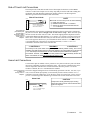
6250 Servo Controller
User Guide
Compumotor Division
Parker Hannifin Corporation
p/n 88-013413-01B October 18, 1993
Important User Information
To ensure that the equipment described in this user guide, as well as all the equipment connected to and used with it, operates
satisfactorily and safely, all applicable local and national codes that apply to installing and operating the equipment must be
followed. Since codes can vary geographically and can change with time, it is the user's responsibility to identify and comply with
the applicable standards and codes. WARNING: Failure to comply with applicable codes and standards can result in
damage to equipment and/or serious injury to personnel.
Personnel who are to install and operate the equipment should study this user guide and all referenced documentation prior to
installation and/or operation of the equipment.
In no event will the provider of the equipment be liable for any incidental, consequential, or special damages of any kind or nature
whatsoever, including but not limited to lost profits arising from or in any way connected with the use of this user guide or the
equipment.
© Compumotor Division of Parker Hannifin Corporation, 1993
— All Rights Reserved —
The information in this user guide, including any apparatus, methods, techniques, and concepts described herein, are the
proprietary property of Parker Compumotor or its licensors, and may not be copied, disclosed, or used for any purpose not expressly
authorized by the owner thereof.
Since Parker Compumotor constantly strives to improve all of its products, we reserve the right to change this user guide and
equipment mentioned therein at any time without notice.
For assistance in the United States, contact:
For assistance in Europe, contact:
Compumotor Division of Parker Hannifin
5500 Business Park Drive
Rohnert Park, CA 94928
Telephone: (800) 358-9070
Fax: (707) 584-8015
Parker Digiplan
21 Balena Close
Poole, Dorset
England BH17 7DX
Telephone: 0202-690911
Fax: 0202-600820
Compumotor
6250 Servo Controller User Guide
Revision B Change Summary
The following is a summary of the primary technical changes to this user guide since the last version was released.
This user guide, p/n 88-013413-01B (released on October 18, 1993), supersedes 88-013413-01A.
Topic
De s c ript ion
S e e Als o
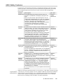
6250-ANI Analog Input Option
is Released
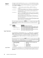
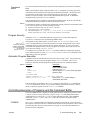
New Option/Feature: The 6250-ANI option was released at the same
time this user guide revision B was released. The -ANI option is a ±10V, 14bit analog input (with anti-aliasing filter) that is sampled at the servo update
rate (set with the SSFR command). One ANI input terminal is located on each
DRIVE connector. The input value can be transferred to the terminal with the
TANI command, or used in a assignment or comparison operation using the
[ANI] command (e.g., VAR1=1ANI). The TANI and [ANI] commands are
used only by the -ANI option, not the standard 6250.
New Feature (see Program Debugging below)
Clarification: While in the continuous mode (MC1), one of the factors that
can stop motion is if the load trips a switch for a general-purpose input that is
configured as a Kill input (INFNCi-C) or a Stop input (INFNCi-D).
Clarification: You must enable the input functions with the INFEN1
command before the drive fault input will be recognized. Also, be sure to set
the drive fault level (DRFLVL) appropriately for the drive you are using.
Clarification: The Compumotor E Series incremental encoders all have
the same cable color codes.
Clarification: When an error occurs, the controller will GOTO or GOSUB,
depending on the error condition (an error resolution table is provided).
Clarification: After the homing operation is successfully completed, the
absolute position register is reset to zero.
New Feature: The INDEB command has been included to allow you to set
the debounce time for the 24 general-purpose programmable inputs and the 2
trigger inputs. The range is 1 - 250 ms, in even increments. The default
debounce time is 4 ms for the 24 inputs, and 25 ms for the trigger inputs.
Correction: The power connection drawing was misleading by stating the
AC input power range was 100 - 120VAC; it is actually 85 - 240VAC.
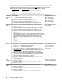
Clarifications:
Deceleration after a stop input or command—In all variations of the COMEXS
mode, upon receiving a stop input or stop command, motion will decelerate at
the preset AD/ADA value.
Resuming after a stop or pause—In the COMEXR1 & COMEXS1 modes, you can
resume program execution and/or motion with a !C command or the pause/
resume input (INFNCi-E) only after the move in progress is completed.
New Features & Clarifications:
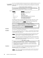
Simulating Analog Input Voltages: (new feature) A new feature called
Analog Voltage Override (enabled with the ANVOEN command and
programmed with the ANVO command) allows you to simulate a voltage on the
analog input channels (input channels 1 - 3 on the JOYSTICK connector).
Programming Error Messages: (clarification) The 6200 can display error
messages and/or a error prompt (?), depending on which error level is
selected with the ERRLVL command. The default error level (ERRLVL4)
displays both the message and the error prompt).
Identifying Bad Commands: (new feature) When the 6200 detects an error
with a command, you can issue the TCMDER command to find out which
command caused the error. This is especially useful when downloading a
program.
New Feature: The JUMP command was added to allow an unconditional
branch to another program and not return. The reason program control does
not return is because all nested IF, WHILE and REPEAT statements, loops,
and subroutines are cleared.
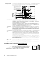
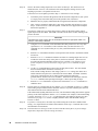
Pg. 16, 54 &
68
Analog Voltage Override
Continuous Mode
Drive Fault Monitoring
Encoders
Error Handling
Homing
Inputs:
Debounce Time
Power Input (AC)
Program & Command Buffer
Execution Control
Program Debugging
Program Flow Control
Pg. 67 & 95
Pg. 53
Pg. 19, 58 &
102
Pg. 12 & 103
Pg. 98
Pg. 49
Pg. 58 & 61
Pg. 5
Pg. 86
Pg. 60-61 &
86-87
Pg. 67 & 95
Pg. 97
Pg. 97
Pg. 88
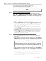
6250 User Guide Change Summary (continued)
Programming:
Troubleshooting problems
RMAs
RP240
Software Revision 1.1
Released
Variable Type Conversion
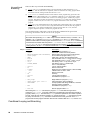
Clarification: In Chapter 7, three resolutions were added to resolve the
following problem situations:
• Start-up program (STARTP) will not run on power up
• Program execution stops at the INFEN1 command
• First time a program is run, the move distances are incorrect, but after
downloading the program a second time the move distances are correct.
Clarification: If you need to return a Compumotor product to affect
repairs or upgrades, be sure to ship it to Suite D at the Rohnert Park
address.
New Features and Clarifications:
Data Read Immediate Mode: (new feature) The DREADI1 command allows
continual input from the RP240 numeric keypad or the function keys (when
used in conjunction with DREAD and/or DREADF). Standard RP240 menus
should not be used in this mode. Data can be read into numeric variables
only. Do not assign the same variable to read numeric and function key data.
Power-up (default) Mode: (clarification) On power up, the 6200 defaults to a
mode in which it controls the RP240 with the menu-driven functions listed on
page 50. To disable this menu, the power-up program (STARTP) must contain
the DCLEARØ command.
This version of the user guide was released at the same time that revision
1.1 of the 6250 software was released.
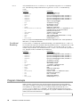
New Feature: The VCVT( ) command has been added to allow you to
convert between variables (numeric-to-binary and binary-to-numeric).
Pg. 108-109
Pg. 110
Pg. 91
Pg. 70
n/a
Pg. 73
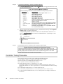
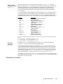
T A B L E
O F
C O N T E N T S
O v e r v i e w . . . . . . . . . . . . . . . . . . . . . . . . . . . . . . . . . . . . . . . . . . . . . . . . . . . . . . . . . . . . . . . . . . . . . . . . . . . . . . . . . . . . . . . . . . . . . . . . . . . . . . . . . . . iii
Assumptions................................................................................................................................. iii
Contents of This User Guide............................................................................................................. iii
Installation Process Overview .......................................................................................................... iv
Conventions ................................................................................................................................. iv
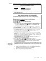
Chapter 1: Introduction . . . . . . . . . . . . . . . . . . . . . . . . . . . . . . . . . . . . . . . . . . . . . . . . . . . . . . . . . . . . . . . . . . . . . . . . . . . . . . . . . . . . . . . 1
6250 Description............................................................................................................................1
6250 Features ............................................................................................................................... 2
Chapter 2: Getting Started . . . . . . . . . . . . . . . . . . . . . . . . . . . . . . . . . . . . . . . . . . . . . . . . . . . . . . . . . . . . . . . . . . . . . . . . . . . . . . . . . . . 3
Inspect The Shipment ..................................................................................................................... 3
Bench Test ................................................................................................................................... 4
➀ RS-232C Communications ............................................................................................... 4
➁ Connect Power Cable ..................................................................................................... 5
➂ Test Procedure ............................................................................................................. 5
Chapter 3: Installation . . . . . . . . . . . . . . . . . . . . . . . . . . . . . . . . . . . . . . . . . . . . . . . . . . . . . . . . . . . . . . . . . . . . . . . . . . . . . . . . . . . . . . . . 7
Installation Precautions .................................................................................................................. 7
➀ Mount the 6250 ......................................................................................................................... 8
➁ System Connections .................................................................................................................. 9
Motor Driver Connections .................................................................................................... 9
End-of-Travel Limit Connections ........................................................................................... 11
Home Limit Connections ...................................................................................................... 11
Encoder Connections ......................................................................................................... 12
Auxiliary +5V Output Connection........................................................................................... 12
Output and Input Pull-up Connections .................................................................................... 12
Enable Input Connection ..................................................................................................... 13
Programmable Inputs & Outputs Connections.......................................................................... 13
Trigger Input Connections.................................................................................................... 14
RP240 Front Panel Connections............................................................................................ 15
Joystick and Analog Input Connections.................................................................................. 15
ANI Analog Input Connections (6250-ANI Option Only).............................................................. 16
Extending 6250 System Cables ............................................................................................ 17
➂ Installation Verification ............................................................................................................... 17
➃ What's Next? ............................................................................................................................ 19
Chapter 4: Servo Tuning . . . . . . . . . . . . . . . . . . . . . . . . . . . . . . . . . . . . . . . . . . . . . . . . . . . . . . . . . . . . . . . . . . . . . . . . . . . . . . . . . . . . . . 2 1
Servo System Terminology .............................................................................................................. 21
Servo Tuning Terminology.................................................................................................... 21
Position Variable Terminology............................................................................................... 22
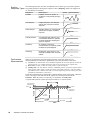
Servo Response Terminology ............................................................................................... 23
6000 Series Servo Commands .......................................................................................................... 25
Servo Control Techniques................................................................................................................ 26
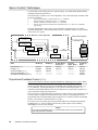
Proportional Feedback Control (SGP)..................................................................................... 26
Integral Feedback Control (SGI)............................................................................................ 27
Velocity Feedback Control (SGV) .......................................................................................... 28
Velocity Feedforward Control (SGVF)..................................................................................... 28
Acceleration Feedforward Control (SGAF) ............................................................................... 28
Tuning Setup Procedure .................................................................................................................. 29
Drive Tuning Procedure (Velocity Drives Only) ..................................................................................... 31
Controller Tuning Procedure ............................................................................................................. 32
Tuning Scenario............................................................................................................................. 38
Target Zone (Move Completion Criteria) .............................................................................................. 40
Chapter 5: Basic 6250 Features . . . . . . . . . . . . . . . . . . . . . . . . . . . . . . . . . . . . . . . . . . . . . . . . . . . . . . . . . . . . . . . . . . . . . . . . . . . . . 4 3
Before You Proceed With This Chapter ............................................................................................... 43
6000 Series Software Reference Guide .................................................................................. 43
Compumotor Bulletin Board Service ....................................................................................... 44
Basic Motion Control Concepts ............................................................................................. 44
Support Software ........................................................................................................................... 44
6000 DOS Support Disk....................................................................................................... 44
Motion Architect® .............................................................................................................. 44
6250 Safety Features ..................................................................................................................... 45
Scaling ........................................................................................................................................ 46
Acceleration & Deceleration Scaling (SCLA/PSCLA) ................................................................. 46
Velocity Scaling (SCLV/PSCLV)............................................................................................ 46
Distance Scaling (SCLD) ..................................................................................................... 47
End-of-Travel Limits ....................................................................................................................... 48
Homing ........................................................................................................................................ 48
Positioning Modes.......................................................................................................................... 51
Preset Mode ..................................................................................................................... 52
Continuous Mode ............................................................................................................... 53
User Interface Options.................................................................................................................... 54
Programmable Inputs and Outputs .................................................................................................... 55
Output Functions ............................................................................................................... 55
Input Functions ................................................................................................................. 58
Thumbwheel Interface......................................................................................................... 63
PLC Interface.................................................................................................................... 65
Joystick Interface.......................................................................................................................... 65
-ANI 14-Bit Analog Input Option (6250-ANI Option Only) ........................................................................ 68
RP240 Front Panel Interface ............................................................................................................ 68
Operator Interface Features................................................................................................. 69
Using the Default Mode ....................................................................................................... 70
Host Computer Operation ................................................................................................................ 72
Variables (Binary, Numeric, and String) .............................................................................................. 73
RS-232C Daisy-Chaining ................................................................................................................. 76
Chapter 6: A d v a n c e d
6250
Features........................................................................ 7 9
S-Curve Profiling............................................................................................................................ 79
X-Y Linear Interpolation................................................................................................................... 81
Chapter 7: 6 2 5 0
Programming
Tips.......................................................................... 8 3
Creating Programs & Subroutines...................................................................................................... 83
Subroutines ...................................................................................................................... 84
Stored Programs and Non-volatile Memory.............................................................................. 84
Automatic Program Execution .............................................................................................. 85
Controlling Execution of Programs and the Command Buffer................................................................... 85
Program Flow Control ...................................................................................................................... 87
Unconditional Looping and Branching..................................................................................... 87
Conditional Looping and Branching ........................................................................................ 89
Program Interrupts ......................................................................................................................... 92
Program Debug Tools......................................................................................................................93
Trace Mode....................................................................................................................... 93
Single-Step Mode............................................................................................................... 94
Simulating Analog Input Channel Voltages .............................................................................. 95
Simulating I/O Activation ..................................................................................................... 95
Programming Error Responses ............................................................................................. 97
Error Handling ............................................................................................................................... 98
Chapter 8: Hardware Reference . . . . . . . . . . . . . . . . . . . . . . . . . . . . . . . . . . . . . . . . . . . . . . . . . . . . . . . . . . . . . . . . . . . . . . . . . . . . . 1 0 1
General Specifications.................................................................................................................... 101
I/O Pin Outs & Circuit Drawings......................................................................................................... 102
Optional DIP Switch Settings............................................................................................................ 105
Chapter 9: Troubleshooting . . . . . . . . . . . . . . . . . . . . . . . . . . . . . . . . . . . . . . . . . . . . . . . . . . . . . . . . . . . . . . . . . . . . . . . . . . . . . . . . . . 1 0 7
Troubleshooting............................................................................................................................. 107
Common Problems & Solutions ............................................................................................. 108
RS-232C Troubleshooting ................................................................................................................ 109
Returning the System ..................................................................................................................... 110
Appendix A: Reducing Electrical Noise . . . . . . . . . . . . . . . . . . . . . . . . . . . . . . . . . . . . . . . . . . . . . . . . . . . . . . . . . . . . . . . . . . . . . 1 1 1
Appendix B: Alphabetical Command List . . . . . . . . . . . . . . . . . . . . . . . . . . . . . . . . . . . . . . . . . . . . . . . . . . . . . . . . . . . . . . . . . . . . 1 1 3
Appendix C: I n d e x . . . . . . . . . . . . . . . . . . . . . . . . . . . . . . . . . . . . . . . . . . . . . . . . . . . . . . . . . . . . . . . . . . . . . . . . . . . . . . . . . . . . . . . . . . . . . . 1 1 7
ii
6250 Servo Controller User Guide
O
V
E
R
V
I
E
W
This user guide is designed to help you install, develop, and maintain your system. This
section is intended to help you find and use the information in this user guide.
Assumptions
To effectively use this user guide to install, develop, and maintain your system, you should
have a fundamental understanding of the following:
❏
❏
❏
Basic electronics concepts (voltage, switches, current, etc.)
Basic motion control concepts (torque, velocity, distance, force, etc.)
Basic programming skills (any high-level language such as BASIC, Fortran, or Pascal)
Contents of This User Guide
Chapter
Purpose
➀
➁
Introduction
Describes the 6250 and provides a brief account of its features.
Getting Started
Lists and describes the items you should have received with your
6250 shipment. A bench test procedure is provided to verify the
system's basic functionality.
➂
Installation
Provides instructions for mounting, wiring up, and testing the
6250 system. Complete all instructions in Chapter 3 before
tuning the 6250 in Chapter 4. Refer to the 6000 Series
Software Reference Guide for detailed descriptions of the
6000 Series commands used in Chapters 4 through 7.
➃
Servo Tuning
Instructs you on how to tune the 6250 for your application.
Sample applications are provided. Complete all tuning
instructions before implementing motion features.
➄
Basic 6250 Features
Describes the 6250's basic user features and instructs you on
how to implement them in your application. Sample applications
are provided.
➅
Advanced 6250 Features
Describes the 6250's advanced user features (S-Curve Profiling,
Linear Interpolation) and instructs you on how to implement them
in your application. Sample applications are provided.
➆
Programming Tips
Instructs you on how to implement the 6250's programming
language in your application.
➇
Hardware Reference
Use the Hardware Reference as a quick-reference tool for 6250
electrical specifications, optional DIP switch settings (address &
baud rate), and I/O signal descriptions and circuit drawings.
➈
Troubleshooting
Describes methods for isolating and resolving hardware and
software problems.
Appendices
A:
B:
C:
Reducing electrical noise in your application
Alphabetical listing of the 6250's commands
Index
Overview
iii
Installation Process Overview
➀
➁
➂
➃
➄
➅
➆
Review this entire user guide. Become familiar with the user guide's contents so that you can
quickly find the information you need. At times you may want to refer to the 6000 Series
Software Reference Guide for detailed descriptions of the 6000 Series commands used in
this user guide.
Read Chapter 1, Introduction, and the user documentation for all peripheral system components
to develop a basic understanding of all system components, their functions, and
interrelationships.
Read Chapter 2, Bench Test, and verify that you have received all the proper components for
your system, and that all the items in your shipment have arrived without damage. Follow the
step-by-step bench test procedures to verify the 6250's basic operability, as well as the
functionality of the host computer (or terminal).
Complete the system configuration, mounting, and wiring instructions provided in Chapter 3,
Installation. Do not deviate from the sequence or installation methods
provided.
While in Chapter 3, be sure to use the Installation Verification procedures to check all the
system functions and features to ensure that you have completed the installation process
correctly.
After you successfully complete all procedures in Chapter 3, you will be ready to proceed to
Chapter 4, Servo Tuning, to tune the drive and the 6250 for your application. The tuning
procedures in Chapter 4 are based primarily on using the Servo Tuner option for Motion
Architect.
After successfully completing all procedures in Chapter 4, you may proceed to Chapters 5
through 7 to implement the 6250's user features in your application.
Conventions
Clockwise (CW, +) & Counter-clockwise (CCW, -) Directions
Clockwise
(CW, +)
Counter-clockwise
(CCW, -)
Throughout this user guide and the 6000 Series Software Reference Guide, you will
find references to the clockwise (CW) and counter-clockwise (CCW) direction of motion. The
CW or CCW direction is determined either by the direction the motor shaft (see illustration at
left), or by the sign (+ or -) of the commanded position (e.g., the D+8ØØØ distance command
indicates a 8,000-unit move in the clockwise direction). This convention is accurate only if
you connect the drive and encoder as described in Chapter 3.
6000 Series Commands
The command language conventions are provided in the 6000 Series Software
Reference Guide. Because some 6000 Series products have four-axis capability, the syntax
of the example commands in the Reference Guide shows data fields for all four axes; ignore
the third and fourth data fields when entering commands or reading status commands for the
6250.
Related Publications
iv
❏
6000 Series Software Reference Guide, Parker Hannifin Corporation, Compumotor
Division; part number 88-012966-01
❏
Motion Architect User Guide, Parker Hannifin Corporation, Compumotor Division; part
number 88-013056-01
❏
Current Parker Compumotor Motion Control Catalog
❏
Schram, Peter (editor). The National Electric Code Handbook (Third Edition). Quincy, MA:
National Fire Protection Association
6250 Servo Controller User Guide
C
H
A
P
T
E
R
➀
Introduction
This chapter describes the 6250's basic functions & features.
6250 Description
The Compumotor 6250 is a stand-alone, two-axis servo controller. The 6250 provides
sophisticated two-axis control of any standard ±10V analog input servo drive system.
The 6250 implements a dual processor approach, comprising a microprocessor for executing
high-level motion programs and a digital signal processor (DSP) for high-speed, sophisticated
servo control. This dual processor approach allows commands to be executed faster.
Using the 6000 Series Programming Language, you can program the 6250 via a PC or a
dumb terminal. User programs are stored in the 6250's battery-backed RAM.
The 6250 also provides operator interface capabilities when used with the Compumotor
RP240 Front Panel.
The 6250 comes standard with support software for the Microsoft® Windows™ and DOS
operating environments:
❏
❏
Motion Architect® is an innovative, easy-to-use Microsoft® Windows™ based programming
aide to help you easily create and implement complex motion programs. The Servo Tuner
option, a special add-on module sold separately, allows you to visually gather data and tune
your controller/drive system. For more information, refer to the Motion Architect User
Guide.
The 6000 DOS Support Disk contains a DOS-based program editor and terminal emulator package.
Also included are sample 6000 Command Language programs.
Additional 6250 features are listed below in the 6250 Features section.
➀ Introduction
1
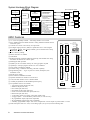
System Hardware Block Diagram
Computer
or
Dumb Terminal
6250
Up to 2 Axes of control
Battery-backed
RAM
for
user programs
RS-232C
Interface
Front Panel
Interface
Optional ±10V,
14-bit Analog Input
Drive #1
Motor #1
Drive #2
Motion
Chip
Axis #1
RP240
Front Panel
Drive Interface
- ±10V Analog Output
- Shutdown Output
- Drive Fault Input
Motion
Chip
Axis #2
Operating System
-----------Microprocessor
68000 - 12MHz
Dual Port RAM
6250-ANI
Option
DSP
- Inc. Encoder Interface
- Position Latch
- Output on Position
Limits
- CW & CCW End-of-travel
- Home
I/O
- Enable Input
- 2 Positon Latch Inputs
- 24 Prog. Inputs
- 24 Prog. Outputs
- 2 Auxiliary Prog. Outputs
Joystick Interface
Motor #2
Limit
Connections
I/O
Connections
Encoder
#1
Encoder
#2
Joystick
6250 Features
❏ 1 to 2 axes of optically isolated —10V analog interface servo control
❏ Servo feedback from incremental encoders. Analog feedback available with the
GRN : READY
STATUS
DRIVE 1
ENCODER 1
RED : RESET
6250-ANI option.
SHLD
+5V
DRIVE1 OFF
❏ Controls servo drives in the velocity or torque mode
COM
A+
DRIVE2 OFF
SHTNC
A❏ Fast digital signal processor (DSP) for sophisticated servo control (digital
SHTNO
B+
DFT
BProportional, Integral, and Velocity feedback, plus acceleration and velocity
AGND
Z+
ANI
ZFeedforward—PIV&F)
CMDGND
2-AXIS SERVO
CMD+
SHLD
CONTROLLER
❏ S-curve motion profiling
®
DRIVE 2
ENCODER 2
LIM 1/2
❏ Motion Architect is standard
SHLD
+5V
1CW
COM
A+
1CCW
❏ Teach Mode
SHTNC
A1HOM
SHTNO
B+
GND
❏ Windows™-based visual data gathering and tuning aide available when using
DFT
B2CW
AGND
Z+
2CCW
the Motion Architect® Servo Tuner option
ANI
Z2HOM
CMDGND
GND
❏ DOS Support Disk provided
CMD+
SHLD
SHLD
❏ 40,000 bytes of non-volatile memory for storing programs & paths
AUX
RP240
❏ Capability to interrupt program execution on error conditions
Rx
+5V
P
P
Tx
GND
R
❏ 2-axis linear interpolation standard
R
GND
Rx
O
O
SHLD
Tx
G
G
❏ Variable storage, conditional branching, and math capability
+5V
SHLD
R
R
A
OUT-P
A
❏ Program debug tools — single-step and trace modes, breakpoints, and
M
M
IN-P
M
M
TRG-A
simulation of I/O
A
A
TRG-B
B
B
J
L
GND
L
❏ Internal power supply
O
E
E
OUT-A
Y
OUT-B
S
❏ Direct interface to RP240 Front Panel
O
I
T
GND
U
N
I
ENBL
T
❏ Operates stand-alone or interfaces to PCs & PLCs
P
C
P
U
K
U
T
❏ 3-wire, RS-232C interface to PC or dumb terminal
T
S
S
❏ 1.2 MHz pre-quadrature encoder feedback pulse frequency
POWER
❏ I/O capabilities (all I/O are isolated):
EARTH N/A
• ±10V analog control output (both axes )
NEUT LINE
Compumotor
• Shutdown output (both axes)
• Drive Fault input (both axes)
6250 Front Panel
• Incremental encoder input (both axes)
• CW & CCW end-of-travel limit inputs (both axes)
• Home limit input (both axes)
• 3 8-bit analog inputs for joystick control and variable input
• 2 (trigger) inputs — use for hardware position latch (±1 count accuracy)
• 24 programmable inputs (Opto-22™ compatible)
• 24 programmable outputs (Opto-22™ compatible)
• 2 auxiliary programmable outputs that can be configured for accurate output on position within ±1 count
❏ 6250-ANI Option offers two ±10V, 14-bit analog inputs (one per axis) with anti-aliasing filter.
6250
2
6250 Servo Controller User Guide
C
H
A
P
T
E
R
➁
Getting Started
The information in this chapter will enable you to:
❏
Verify that each component of your 6250 system has been delivered safely and configured
properly
❏
Bench test the 6250's power and RS-232C interface to the host computer/terminal
Inspect The Shipment
If you need to return
any or all of the 6250
system components,
use the return
procedures in Chapter
9, Troubleshooting.
You should inspect your 6250 shipment upon receipt for obvious damage to its shipping
container. Report any damage to the shipping company as soon as possible. Parker
Compumotor cannot be held responsible for damage incurred in shipment. The items listed
below should be present and in good condition.
Part
Part Number
6250 main unit (w/ship kit)
Ship kit: 6250 Servo Controller User Guide
6250 (or 6250-ANI, if so ordered *)
88-013413-01
88-012966-01
95-013070-01
95-013070-02
95-013714-01
88-013056-01
95-012266-01
88-013258-01
71-009039-01
6000 Series Software Reference Guide
Motion Architect® diskettes
Motion Architect Servo Tuner diskette (optional)
Motion Architect User Guide
DOS Support Disk
DOS Support Disk Quick Reference
8-foot AC power cord
* The 6250-ANI is an optional version of the 6250 which provides two ±10V, 14-bit analog inputs. If you ordered a
-ANI option, check the serial tag on the side of the 6250's chassis; it should say 6250-ANI.
Pre-Wired Connections
You should receive your 6250 with the following connections on the AUX connector prewired
(from the factory):
AUX
+5V supplies power to OUT-P and IN-P.
This provides power to the output and input pull-ups.
If this connection is broken, the 6250's
analog command output signal is held
to zero volts (independent of the DSP
and microprocessor).
Rx
Tx
GND
SHLD
+5V
OUT-P
IN-P
TRG-A
TRG-B
GND
OUT-A
OUT-B
GND
ENBL
❏
Output and input pull-ups
(OUT-P and IN-P) connected
to the +5V power supply (+5V)
❏
Enable input (ENBL)
connected to ground (GND)
➁ Getting Started
3
Bench Test
This section leads you through step-by-step instructions to bench test your 6250 system.
This is a temporary (bench top) configuration; the permanent installation will be performed in
Chapter 3, Installation. In this section, you will complete the following tasks:
➀
➁
➂
RS-232C Communications
Connect Power Cable
Test Procedure
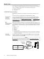
➀ RS-232C Communications
To communicate with the 6250, your computer or terminal must have an RS-232C serial
port.
The 6250 uses a three-wire implementation of standard EIA RS-232C signals.
Computer-toTerminal
Conversion
If you are using an IBM/compatible computer, you must use a terminal emulator software
package to communicate with the 6250. The 6250 comes standard with Motion Architect®
for Windows™ and the 6000 DOS Support Disk; both provide a terminal emulator and
program editor (refer to the Motion Architect User Guide or the 6000 DOS Support
Disk Quick Reference for installation and other user information). You may also use
communication programs such as Crosstalk™, PC-Talk™, and PROCOMM™.
Set
Communication
Parameters
Make sure your computer or terminal is set to the following communication parameters. You
can configure these parameters by using one of the terminal emulation software packages listed
above in Computer-to-Terminal Conversion. If you are using Motion Architect® or the 6000
DOS Support Disk, verify that the baud rate, data bit, parity, and stop bit parameters are set as
follows:
Terminal
Connections
❏
❏
❏
❏
❏
❏
Baud Rate: 9600*
Data Bits: 8
Parity: None
Stop Bits: 1
Full Duplex
XON/XOFF: Enabled
*
If your terminal is not capable of 9600 baud, use the 6250's auto-baud function to automatically
set the 6250's baud rate equal to the terminal's baud rate. Refer to Optional DIP Switch Settings
in Chapter 8 for instructions.
The Receive Data (Rx), Transmit Data (Tx), and Ground (GND) signals are on the 6250's AUX
connector (shown below). The ground (GND) connection on the connector is signal ground or
common as opposed to earth ground (SHLD).
NOTE
If you intend to daisy chain multiple 6250 servo controllers, do not attempt the daisy-chain
connections now. Daisy-chain instructions are provided in Chapter 5, Basic 6250 Features.
AUX
Computer or
Terminal
(Serial Port)
Standard 9-Pin
COM Port Pin Outs:
Pin 3 = Transmit (Tx)
Pin 2 = Receive (Rx)
Pin 5 = Ground (GND)
4
6250 Servo Controller User Guide
Standard 25-Pin
COM Port Pin Outs:
Pin 2 = Transmit (Tx)
Pin 3 = Receive (Rx)
Pin 7 = Ground (GND)
Tx
Rx
GND
Rx
Tx
GND
SHLD
+5V
OUT-P
IN-P
TRG-A
TRG-B
GND
OUT-A
OUT-B
GND
ENBL
➁ Connect Power Cable
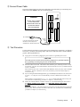
The 6250 is shipped with an 8-foot power cable that is prewired and keyed. Attach the power
cable to the 6250's POWER connector as illustrated below.
WARNING
2-AXIS SERVO
CONTROLLER
DO NOT APPLY POWER
TO THE 6250 UNTIL
INSTRUCTED TO DO SO
IN THE FOLLOWING
TEST PROCEDURE.
85 - 240VAC
If you have a power source other than
85-240VAC, refer to Chapter 8 for
specifications on alternative input power.
Protective
Rubber
Boot
POWER
EARTH
NEUT
N/A
LINE
Compumotor
➂ Test Procedure
Use the following procedure to test the 6250's power and RS-232C connections. In Chapter 3,
Installation, you will test the analog output, end-of-travel and home limits, encoders, RP240,
joystick, and programmable I/O.
➀
Apply power to the 6250 by plugging the power cable into a grounded power source.
CAUTION
The earth ground connection must be made by plugging into a grounded receptacle
or by physically connecting the green wire to earth ground.
➁
Watch the LEDs on the 6250. The STATUS LED should be green, indicating the 6250 is ready
for operation. The other two LEDs should be red because the drives are not yet enabled with the
DRIVE11 command.
If the STATUS LED is red, or if none of the LEDs illuminate, check your power source and cable
connections. If these connections seem correct, disconnect power and consult Chapter 9,
Troubleshooting.
➂
If you are using the 6000 DOS Support Disk, go to the Set-up menu and move the cursor down
to CHECK OUT and press ENTER to automatically verify the communication interface to the
6250.
If the interface is not successful (Device not Ready message will flash on the screen), refer
to the RS-232C troubleshooting procedures in Chapter 9, Troubleshooting.
➃
Initiate the terminal emulator in Motion Architect or in the 6000 DOS Support Disk (refer to
the Motion Architect User Guide or the 6000 DOS Support Disk Quick
Reference if necessary). You could also use your own terminal emulator package.
Press the RETURN key. The cursor should move down one or two lines each time you press the
RETURN key. If the cursor does not move as described, refer to the RS-232C troubleshooting
procedures in Chapter 9, Troubleshooting.
➁ Getting Started
5
C
H
A
P
T
E
➂
R
Installation
The information in this chapter will enable you to:
❏
❏
❏
Mount all system components properly
Connect all inputs and outputs properly
Verify that the complete system is installed properly
To ensure proper installation, you should perform all the bench test procedures in Chapter 2,
Getting Started, before proceeding with the permanent installation process in this chapter.
Installation Precautions
To help ensure personal safety and long life of system components, pay special attention to
the following installation precautions.
WARNING
Always remove power to the 6250 before performing wiring installation or changing DIP switch
settings.
Heat & Humidity
Operate the 6250 system at an ambient temperature between 32° and 122°F (0° to 50°C). Keep
the relative humidity below 95%.
Electrical Noise
Minimize the potential for electrical noise before installing the 6250, rather than attempting to
solve such problems after installation. You can prevent electrical noise by observing the
following installation precautions:
For more information
on electrical noise,
refer to Appendix A.
❏
❏
❏
Do not route high-voltage wires and low-level signals in the same conduit.
Ensure that all components are properly grounded.
Ensure that all wiring is properly shielded.
➂ Installation
7
Airborne Contaminants
Contaminants that may come in contact with the 6250 should be carefully controlled.
Particulate contaminants, especially electrically conductive material such as metal shavings,
can damage the 6250.
Follow Installation Procedure
To ensure proper installation of the 6250 system, this chapter is organized in logical, linear
steps. Deviating from this prescribed format may result in system problems.
➀ Mount the 6250 Servo Controller
➁ Perform system connections
➂ Perform the system test
➀
Mount the 6250
The 6250 should be installed in an enclosure that will protect it from atmospheric
contaminants such as oil, metal, moisture, and dirt. Refer to the National Electrical
Manufacturers Association (NEMA) specifications that pertain to your particular operating
environment. The drawing below illustrates the 6250's dimensions.
4.20 (106.68)
2.70 (68.58)
9.61 (244.10)
0.75 (19.05)
10.00
(254.00)
10.80
(274.32)
11.60
(294.64)
0.80 (20.32)
inches (millimeters)
Provision for #10
Mounting Screws
(4 Plcs.)
0.60 (15.25)
Panel Layout
If you mount the 6250 in an enclosure with other equipment, be sure to maintain at least 2
inches of unrestricted air-flow space around the chassis. The maximum allowable ambient
temperature directly below the 6250 is 122°F (50°C). Fan cooling may be necessary if
adequate air flow is not provided.
➁
System Connections
8
6250 Servo Controller User Guide
This section describes procedures for the following 6250 system connections:
❏
❏
❏
❏
❏
❏
❏
❏
❏
❏
❏
Motor Drivers
End-of-travel and home limits
Encoders
Auxiliary +5VDC output
Output pull-up (OUT-P)
Programmable inputs and outputs (including auxiliary outputs OUT-A and OUT-B)
Trigger inputs (TRG-A and TRG-B)
RP240 Front Panel
Joystick and analog inputs
ANI analog inputs (6250-ANI option only)
Extending cables
Refer to the bench test procedures in Chapter 2 for the following connections:
❏
❏
Power
RS-232C communications
Refer to Chapter 5 for connection procedures on the following:
❏
❏
❏
PLC
Thumbwheels
RS-232C daisy-chain
NOTE
Refer to Chapter 8, Hardware Reference, for system specifications and detailed I/O circuit
drawings and signal descriptions.
Motor Driver Connections
Before you connect the drives to the 6250, configure your drives and connect the motors
according to the user documentation for your drives.
CAUTION
Before connecting to your Motor/Drive system, be sure that power is not applied to the 6250.
The 6250 provides a standard ±10V analog control signal for use with any servo drive. The
following table lists the 6250's motor driver connector pin outs; with this information you
can connect the drives to the 6250's 9-pin screw terminal connectors as illustrated below. I/O
circuit drawings are provided in Chapter 8, Hardware Reference.
Pin #
Name
In/Out
Description
1
2
3
SHLD
COM
SHTNC
--------OUT
4
SHTNO
OUT
5
6
7
8
9
DFT
AGND
ANI
CMDCMD+
IN
----IN
OUT
OUT
Shield—internally connect to chassis (earth) ground.
Signal common for shutdown.
Shutdown relay output to drives that require a closed contact to disable the drive.
The shutdown relay is active (disabling the drive) when no power is applied to
the 6250. When the 6250 is powered up, the shutdown relay remains active until
you issue the DRIVE11 command.
Shutdown active (DRIVEØØ): this output is internally connected to COM.
Shutdown inactive (DRIVE11): this output is disconnected from COM.
Shutdown relay output to drives that require an open contact to disable the drive.
The shutdown relay is active (disabling the drive) when no power is applied to
the 6250. When the 6250 is powered up, the shutdown relay remains active until
you issue the DRIVE11 command.
Shutdown active (DRIVEØØ): this output is disconnected from COM.
Shutdown inactive (DRIVE11): this output is internally connected to COM.
Drive fault input. Set active level with the DRFLVL command.
Analog ground.
±10V, 14-Bit analog input (available only with the 6250-ANI option).
Command signal return.
Command output signal (±10V signal).
➂ Installation
9
<<WARNING>>
SAFETY FIRST
<<WARNING>>
If your drive does not have a shutdown input, install a manual emergency-stop switch for the drive's power supply.
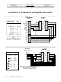
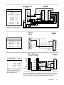
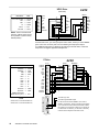
Connections to Compumotor and Digiplan Servo Drives
APEX Series
Drive
6250
DRIVE 1
APEX Series Drive
A+
A–
SRVON
Voc
B+
B–
Z+
Z–
VIN
AGND
(pin 13)
(pin 14)
(pin 23)
(pin 24)
(pin 29)
(pin 30)
(pin 43)
(pin 44)
(pin 49)
(pin 50)
Reset
Gnd
Vel Int Enable
Enable In
Fault Out
Gnd
Command+
Command–
Tach Output
Gnd
+15V
Gnd
-15V
6250
↔
↔
↔
↔
↔
↔
↔
↔
↔
↔
A–
A+
SHTNO
+5V
B+
B–
Z+
Z–
CMD+
CMD–
NOTE:
Apex Series A+ connected to 6250’s A–
Apex Series A– connected to 6250’s A+
ENCODER 1
SHLD
COM
SHTNC
SHTNO
DFT
AGND
ANI
CMDCMD+
CHA+
CHA–
CHB+
CHB–
CHZ+
CHZ–
Gnd
BL Drive
User I/O Connector
6250
DRIVE 1
BL Drive
V2 (pin 1)
V1 (pin 2)
GND (pin 4)
RST (pin 5)
+15V (pin 6)
FT (pin 9)
AOP (pin 10)
AOP (pin 11)
BOP (pin 12)
BOP (pin 13)
ZOP (pin 14)
ZOP (pin 15)
10
15
6250
↔
↔
↔
↔
↔
↔
↔
↔
↔
↔
↔
↔
CMD–
CMD+
GND
COM
SHTNO
DFT
A–
A+
B+
B–
Z+
Z–
8
9
1
NOTE: These connections will work only if
BL jumper LK2 is set to position B
(not the factory default position).
6250 Servo Controller User Guide
+5V
A+
A–
B+
B–
Z+
Z–
GND
SHLD
ENCODER 1
SHLD
COM
SHTNC
SHTNO
DFT
AGND
ANI
CMD–
CMD+
+5V
A+
A–
B+
B–
Z+
Z–
GND
SHLD
6250
Dynaserv Drive
DN1
(50-pin Honda Connector)
Dynaserv Drive
6250
1
DRIVE 1
33
SHLD
COM
SHTNC
SHTNO
DFT
AGND
ANI
CMDCMD+
19
A+
A–
SRVON
Voc
B+
B–
Z+
Z–
VIN
AGND
(pin 13)
(pin 14)
(pin 23)
(pin 24)
(pin 29)
(pin 30)
(pin 43)
(pin 44)
(pin 49)
(pin 50)
↔
↔
↔
↔
↔
↔
↔
↔
↔
↔
ENCODER 1
A–
A+
SHTNO
+5V
B+
B–
Z+
Z–
CMD+
CMD–
18
+5V
A+
AB+
BZ+
ZGND
SHLD
50
NOTE:
Dynaserv A+ connected to 6250’s A–
Dynaserv A– connected to 6250’s A+
6250
OEM670
Drive
1
OEM670 Drive
CMD+ (pin 1)
CMD– (pin 2)
FAULT (pin 9)
ENABLE (pin 10)
GND (pin 11)
GND (pin 16)
14
6250
↔
↔
↔
↔
↔
↔
DRIVE 1
CMD+
CMD–
DFT
SHTNO
COM
AGND
SHLD
COM
SHTNC
SHTNO
DFT
AGND
ANI
CMD–
CMD+
25
13
UD2 & UD5 Drives
6250
(UR3, UR4 or UR8 Rack)
PL9
UD2 & UD5 Drives
+15V, LSW1 & LSW2
VEL2
VEL1
0V
FAULT
EXT.DIS
6250
↔
↔
↔
↔
↔
↔
SHTNO
CMD–
CMD+
AGND
DFT
COM
NOTE: These connections will
work only if UD2/5 jumper LK1 is
set to the 0V position (not the
factory default position).
18V AC
0V
18V AC
+15V
0V
–15V
0V
RESET
READY
PSU FAULT
PLB
1
G1
G2
VEL2
VEL1
SCREEN
0V
FAULT
EXT.DIS
LSW1
LSW2
1
DRIVE 1
SHLD
COM
SHTNC
SHTNO
DFT
AGND
ANI
CMD–
CMD+
If a drive fault occurs, you must cycle power to the drives, unless you control RESET
(PL9 pin 8 on UR4 & UR8 racks, PL4 pin 8 on UR3 rack) with one of the 6250’s
general-purpose outputs. For additional instructions on detecting and reacting to UD
rack faults, contact the Compumotor or Digiplan Applications Department.
➂ Installation
11
UD12 Drive
6250
(UR4 Rack)
UD12 Drive
+15V, LSW & LSW2
VEL2
VEL1
0V
FAULT
EXT.DIS
6250
↔
↔
↔
↔
↔
↔
1
SHTNO
CMD–
CMD+
AGND
DFT
SHLD
NOTE: These connections will
work only if UD12 jumper LK3 is
set to position A (not the factory
default position).
1
18V AC
0V
18V AC
+15V
0V
–15V
0V
RESET
READY
PSU FAULT
DRIVE 1
G1
G2
VEL2
VEL1
SCREEN
0V
FAULT
EXT.DIS
LSW1
LSW2
SHLD
COM
SHTNC
SHTNO
DFT
AGND
ANI
CMD–
CMD+
PLnC
PL9A
If a drive fault occurs, you must cycle power to the drives, unless you control RESET
(pin 8 on the PL9 connector) with one of the 6250's general-purpose outputs.
For additional instructions on detecting and reacting to UD rack faults, contact the
Compumotor or Digiplan Applications Department.
Z Drive
I/O [1]
Z Drive
↔
↔
↔
↔
↔
↔
↔
↔
↔
↔
↔
↔
SHTNO
COM
AGND
GND
A–
A+
B+
B–
Z+
Z–
CMD+
CMD–
↔ DFT
NOTE:
Z Drive CHA+ connected to 6250’s A–
Z Drive CHA– connected to 6250’s A+
1
13
12
6250 Servo Controller User Guide
DRIVE 1
ENABLE+
ENABLE–
RTI+
RTI–
RTO+
RTO–
GND
Tx
Rx
GND
CHA+
CHA–
CHB+
CHB–
CHZ+
CHZ–
ANALOG+
ANALOG–
ENCODER 1
SHLD
COM
SHTNC
SHTNO
DFT
AGND
ANI
CMDCMD+
+5V
A+
A–
B+
B–
Z+
Z–
GND
SHLD
14
To 6250 Logic Gnd
INDEXER CONNECTOR
ENABLE+
ENABLE–
GND
GND
CHA+
CHA–
CHB+
CHB–
CHZ+
CHZ–
ANALOG+
ANALOG–
Indexer Connector
DRIVE FAULT (pin 9)
6250
6250
To 6250 Programmable Output
Pin #7 and #19 are FAULT RESET+ and FAULT
RESET– respectively. These connections are required
if you need to clear a drive fault via the 6250. Activate
the output for no longer than 140ms. If you choose not
to make these connections, you will have to manually
reset the Z Drive anytime a drive fault occurs.
25
End-of-Travel Limit Connections
The 6250 provides CCW and CW end-of-travel limit inputs for both axes via the LIM 1/2
connector. End-of-travel inputs serve as safety stops that prevent the load from crashing into
mechanical stops and damaging equipment or injuring personnel. The drawing below
illustrates typical end-of-travel limit switch connections.
End-of-Travel Limits
NOTE
LIM 1/2
1CW
1CCW
1HOM
GND
2CW
2CCW
2HOM
GND
SHLD
Use of hardware
(and software) endof-travel limits is
discussed in detail in
the End-of-Travel
Limits section in
Chapter 5.
Normally-closed switches*
* LHLVL command changes
active level of switches
Motion will not occur until you do one of the following:
❏ Install limit switches
❏ Disable the limits with the LH command
❏ Change the active level of the limits with the
LHLVL command
Mount normally-closed switches such that the load forces them to open before it reaches the
physical travel limit (leave enough room for the load to stop). When the load opens
the limit switch, the motor comes to a halt. The actual stopping distance depends on motor
speed and the Hard Limit Deceleration (LHADA and/or LHAD) setting. The motor will not be
able to move in that same direction until you clear the limit (close the switch) and execute a
move in the opposite direction (or you can disable the limits with the LH command, but this
is recommended only if the motor is not coupled to the load). Use the TLIM or TAS
commands to check the status of the limit switches.
<< CAUTION >>
RUNAWAY
<< CAUTION >>
If a runaway occurs (motor starts moving, usually at the fastest possible velocity, due to servo
instability), the 6250 will shut down the drive if the maximum encoder position error (set with the
SMPER command) is exceeded before an end-of-travel limit (either hardware of software) is
encountered. However, if the maximum encoder position error is not exceeded by the time the
limit is encountered, the 6250 may not be able to stop the motor.
Home Limit Connections
Use the Home input to establish a home position or zero position reference point. The home
input (TTL compatible) is used for homing the motor. The encoder's Z channel pulse can be
used in conjunction with the home switch to determine the home position. To use the
encoder's Z channel, the HOMZ command must be enabled.
Homing is discussed
in detail in the
Homing section in
Chapter 5.
The 6250 is shipped configured for use with normally-open home switches. You can, if you
wish, reverse the home input polarity (to use normally-closed switches) with the HOMLVL
command. The most common way to use the home switch is to mount it at a home reference
position. The drawing below illustrates typical home limit switch connections to the 6250.
Home Limit
LIM 1/2
1CW
1CCW
1HOM
GND
2CW
2CCW
2HOM
GND
SHLD
CAUTION
Compumotor cannot guarantee proper homing
performance with the home and end-of-travel limit
inputs tied together.
Normally-open switch*
* HOMLVL command changes
active level of switch
➂ Installation
13
Encoder Connections
The 6250 supports up to two incremental encoders. If you use encoders other than those
supplied by Compumotor, pay special attention to the following requirements:
❏
❏
Use incremental encoders with two-phase quadrature output. An index or Z channel output is
optional. Differential outputs are recommended.
It must be a 5V encoder to use the 6250's +5V output. Otherwise, it must be separately powered,
with TTL-compatible or open-collector outputs.
The illustration below shows the wiring techniques that you must use to connect encoders to
the 6250. Refer to Chapter 8 for the 6250's encoder input circuit drawing. If you are using the
BL or Dynaserv drives, refer to the connection illustrations earlier in the Motor Driver
Connections section.
ENCODER 1
ENCODER 2
+5V
A+
AB+
BZ+
ZGND
SHLD
+5V
A+
AB+
BZ+
ZGND
SHLD
+5VDC
A Channel +
A Channel B Channel +
B Channel Z Channel +
Z Channel Ground
Shield
Incremental
Encoder
Note for Using Single-Ended Encoders
If you are using a single-ended encoder leave the 6250's A-, B-, and Z- terminals not connected.
Encoder
Connector Pin
Outs
Each axis has a 9-pin Phoenix connector for incremental encoder connections. The pin-out
description for the ENCODER connectors is provided below.
Pin
In/Out
Name
9
8
7
6
5
4
3
2
1
OUT
IN
IN
IN
IN
IN
IN
---------
+5V
A Channel +
A Channel B Channel +
B Channel Z Channel +
Z Channel Ground
Shield
Compumotor E Series
Encoder Cable Colors
Red
Brown
Brown/White
Green
Green/White
Orange
Orange/White
Black
Shield
Description
+5VDC output to power the encoder
A+ channel quadrature signal from encoder
A- channel quadrature signal from encoder
B+ channel quadrature signal from encoder
B- channel quadrature signal from encoder
Z+ channel quadrature signal from encoder
Z- channel quadrature signal from encoder
Isolated logic ground
Internally connected to chassis ground (earth)
Auxiliary +5V Output Connection
The 6250 provides +5VDC output on the AUX, ENCODER, and RP240 connectors. As much as
1.8A is available. 1.8A is sufficient power for the total load on all the I/O connectors. For
example, using two encoders (each drawing 250mA) and one RP240 (drawing 100mA), 1.2A
would be left for other purposes. The drawing below illustrates example connections for
powering the output pull-up.
Output and Input Pull-up Connections
(output pull-up) and IN-P (input
pull-up), located on the AUX connector,
provide power to the outputs and
inputs. The 6250 is shipped from the
factory with OUT-P and IN-P connected
to +5V to power the outputs and inputs
(see illustration at right).
OUT-P
14
6250 Servo Controller User Guide
+5V supplies power to OUT-P and IN-P.
This provides power to the output and input pull-ups.
(As an alternative, you can connect OUT-P and IN-P
to an external power source of up to 24V.)
If this switch is opened, the 6250's analog
command output signal is held to zero volts
(independent of the DSP and microprocessor).
Normally-closed
switch
AUX
Rx
Tx
GND
SHLD
+5V
OUT-P
IN-P
TRG-A
TRG-B
GND
OUT-A
OUT-B
GND
ENBL
Enable Input Connection
The ENBL (enable) input is located on the AUX connector. The 6250 is shipped with ENBL
wired to GND (see drawing) to allow motor motion.
See the illustration above for an example connection using a normally-closed switch.
Opening the switch sets the ±10V analog command output to zero volts and activates the
shutdown outputs; this is done independent of microprocessor and DSP control. The encoder's
position is retained when the ENBL input is activated. If the ENBL input is not grounded when
motion is commanded, the error message WARNING: ENABLE INPUT INACTIVE will be
displayed.
If error bit #9 of the ERROR command is enabled, the error program (ERRORP) will be
executed. You can check the status of the ENBL input with the TINO, INO, TER and ER
commands.
Programmable Inputs & Outputs Connections
The PROGRAMMABLE INPUTS connector provides 24 programmable inputs and the
PROGRAMMABLE OUTPUTS connector provides 24 programmable outputs. Two additional (and
functionally identical) programmable outputs, OUT-A and OUT-B, are available on the AUX
connector. Two additional trigger (position latch) inputs are also available on the AUX
connector, but due to their functional differences they are discussed later in the Triggers
section. All these inputs and outputs are optically isolated and TTL compatible.
All 26 programmable outputs are pulled up using the OUT-P pin on the AUX connector (see
illustration above). The 6250 is factory wired for +5VDC logic. If +5VDC is not to be used,
disconnect OUT-P from the +5V terminal and connect OUT-P to an external supply of up to
24V. Note: Even if you use an external 24V supply the switching thresholds remain TTL
compatible ( ≤ 0.4V = Low,
≥ 2.4 V = High).
Change inputs from
sourcing to sinking.
All 24 programmable inputs are pulled up to +5V by connecting the IN-P terminal to the +5V
terminal on the AUX connector. If you wish to have the inputs sink current instead of source
current, you can connect IN-P to GND. For compatibility with equipment operating at
24VDC, the inputs may be pulled up to 24VDC by using an external power supply. The
trigger inputs (TRG-A & TRG-B) are internally tied to 5V, but can have up to 24V connected to
them.
These I/O are typically used with normally-open or normally-closed switches; however, they
can also be used with I/O module racks, PLCs, and thumbwheels (including the Compumotor
TM8).
If you are using PLCs or thumbwheels, refer to the connection instructions and application
considerations provided in the Programmable Inputs and Outputs section of Chapter 5.
Also provided in the Programmable Inputs and Outputs section are instructions for defining
and controlling programmable inputs and outputs via programs written with the 6000 Series
programming language.
Programmable
I/O Pin Outs
The following table lists the pin outs on the two 50-pin flat cable headers labeled
PROGRAMMABLE INPUTS and PROGRAMMABLE OUTPUTS. Refer to Chapter 8, Hardware
Reference, for internal I/O schematics.
PROGRAMMABLE INPUTS Connector
Pin # Function
Pin # Function
PROGRAMMABLE OUTPUTS Connector
Pin # Function
Pin # Function
49
47
45
43
41
39
37
35
33
31
29
49
47
45
43
41
39
37
35
33
31
29
+5 VDC
Input #1 (LSB)
Input #2
Input #3
Input #4
Input #5
Input #6
Input #7
Input #8
Input #9
Input #10
23
21
19
17
15
13
11
09
07
05
03
Input #13
Input #14
Input #15
Input #16
Input #17
Input #18
Input #19
Input #20
Input #21
Input #22
Input #23
+5 VDC
Output #1 (LSB)
Output #2
Output #3
Output #4
Output #5
Output #6
Output #7
Output #8
Output #9
Output #10
23
21
19
17
15
13
11
09
07
05
03
Output #13
Output #14
Output #15
Output #16
Output #17
Output #18
Output #19
Output #20
Output #21
Output #22
Output #23
➂ Installation
15
27
25
Input #11
Input #12
01
Input #24 (MSB)
27
25
Output #11
Output #12
01
Output #24 (MSB)
NOTE: All even-numbered pins are connected to logic ground (DC ground).
Optional VM50
Adaptor
If you wish to use screw terminal connections for the 24 programmable I/O, Compumotor
offers the VM50 adaptor (p/n VM50). If you wish to use screw terminal connections for both
the 24 inputs and the 24 outputs, you will need two VM50 adaptors.
The pin numbers on the VM50's screw terminals correspond to the same pin outs on the
PROGRAMMABLE INPUTS and PROGRAMMABLE OUTPUTS connectors. The VM50 simply
attaches to the 6250 via the 2-foot, 50-pin ribbon cable that comes with the VM50 (see
drawing below).
To order the VM50, contact your distributor or ATC, or call Compumotor at (800) 722-2282.
6250
Programmable I/O
Connectors
2-Foot Cable
(provided with VM50)
VM50 snaps on to any
standard DIN Rail
2
4
1
6
3
8 10 12 14 16 18 20 22 24 26 28 30 32 34 36 38 40 42 44 46 48 50
5
7
9 11 13 15 17 19 21 23 25 27 29 31 33 35 37 39 41 43 45 47 49
VM50 Adaptor Board
Trigger Input Connections
The 6250 provides two trigger (position latch) inputs. Like the programmable inputs described
earlier, trigger inputs can be connected to PLC outputs, discrete switches, or electronic sensors,
and are monitored under program control. The status of triggers A and B is represented
respectively by bits 25 and 26 in the [IN], INFNC, INLVL, ONIN, and TIN commands.
Using the WAIT command, the 6250 can be programmed to wait until one or more inputs
switch to a desired state before executing the next command.
AUX
Normally-open switches *
* The INLVL command changes the active level of inputs.
Position Latch
Feature
Rx
Tx
GND
SHLD
+5V
OUT-P
IN-P
TRG-A
TRG-B
GND
OUT-A
OUT-B
GND
ENBL
The trigger inputs function identically to the regular 24 programmable inputs, except when
they are programmed with the Trigger Interrupt Function (INFNCi-H) command to function
as position latch inputs.
When configured as position latch inputs, the input enable/disable (INEN) command has no
effect on the trigger inputs. Note: The position latch feature is discussed in the Programmable
Inputs and Outputs section in Chapter 5)
16
6250 Servo Controller User Guide
RP240 Front Panel Connections (RP240 is optional)
Using a four-wire shielded cable, connect the RP240 to the 6250's RP240 connector (see
below). For cable lengths up to 50 feet, use 20 AWG wire (cable lengths longer than 50 feet
are not recommended). Refer to the RP240 User Guide for mounting instructions.
NOTE
For the 6250 to recognize the RP240, the RP240 connection must be made prior to powering up
(or resetting) the 6250. If you connect the RP240 to the 6250 before powering up the 6250, the
6250 will recognize the RP240 and send the *RP24Ø CONNECTED message to the RS-232C
terminal. If the 6250 does not detect a RP240 upon power up or reset, then the following
message will be sent to the RS-232C terminal: *NO REMOTE PANEL.
Connector on back panel Connector on
of RP240
RP240
GND
Rx
Tx
+5V
+5V
GND
Rx
Tx
SHLD
Joystick and Analog Input Connections
You can use the three analog inputs on the JOYSTICK connector for 2-axis joystick control of
the axes, and/or as a low-resolution analog input (8-bit A/D, 1mV/bit) for process control.
The Daedal JS6000 joystick is compatible with the Compumotor 6250. To order the JS6000,
contact Daedal at (800) 245-6903 or contact your local distributor.
Refer to Chapter 5
for a detailed
discussion of joystick
control.
Joystick
Connector
Pin Outs
The input range of the analog input is 0V to 2.5V. A joystick with a linear taper 5KΩ
potentiometer (pot) with 60° of travel is recommended (the pot has 300° of travel, but
typically only 60° is usable with a joystick). The pot should be adjusted so that its resistance
is close to 0Ω when the joystick is all the way to one side, and about 1KΩ when the joystick
is all the way to the other side. Also, connect a 1KΩ resistor between the analog input and
+5V.
The JOYSTICK connector is a 25-pin D connector. The pin-out descriptions are provided in the
table below. The 6250's internal analog input circuit diagram is provided in Chapter 8,
Hardware Reference.
Pin
1
2
3
4
8
14
15
16
In/Out
IN
IN
IN
—
—
—
IN
IN
Name
Analog Channel 1
Analog Channel 2
Analog Channel 3
Unused
Shield
Ground
Axes Select
Velocity Select
17
IN
Joystick Release
18
IN
Joystick Trigger
19
IN
Joystick Auxiliary
23
OUT
+5VDC (out)
Description
8-bit analog input for joystick control of axis (can override with the ANVOEN and ANVO commands)
8-bit analog input for joystick control of axis (can override with the ANVOEN and ANVO commands)
8-bit analog input for joystick control of axis (can override with the ANVOEN and ANVO commands)
--------------Shield
Ground
If only using one analog input, you can use this input to alternately control axes 1 or 2
Input to select high or low velocity range (as defined with JOYVH or JOYVL command)
Input to release the 6250 from joystick mode (JOY). Same as issuing the !JOYØØ command.
Program execution will continue with the first statement after the joystick enable (JOY1) command.
Status of this active-low input can be read by a program (using the INO or TINO commands) to
control program flow, or to enter the 6250 into joystick mode.
Status of this active-low input can be read by a program (using the INO or TINO commands) to
control program flow, or to teach positions to a program.
+5VDC power output
➂ Installation
17
Analog Inputs
You can use the analog inputs for joystick control of the axes. An analog input can command
an axis velocity from full CW to full CCW. The following drawing illustrates a typical
joystick connection example.
Joystick potentiometers are 5KΩ with
60° of usable travel adjusted to span
0Ω to 1KΩ.
*
1KΩ Resistors
*
The 1KΩ resistors for velocity select,
axes select, joystick trigger, & joystick
auxiliary are for noise suppression only.
J
O
Y
S
T
I
C
K
+5VDC
Analog Channel 1
Analog Channel 2
Velocity Select
Axes Select
Joystick Release
Joystick Trigger
23
1
2
16
15
17
18
19
14
8
Joystick
X Axis
Y Axis
5KΩ
5KΩ
N.C. Momentary
Joystick Release
Joystick Auxiliary
GND
Velocity Select
Axes Select
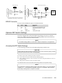
N.O. Momentary
Joystick Trigger
Joystick Aux.
SHLD
Axes Select Input You can define two configurations (JOYAXH and JOYAXL) that define which axes are
controlled by which channels. The axes select input allows you to select the current
configuration. An axes select input high references the JOYAXH command. An axes select
input low references the JOYAXL command.
One possible configuration is as follows: With axes select input high, analog channel #1
controls axis one and analog channel #2 controls axis two (JOYAXH1,2). With axes select
input low, analog channel #3 controls both axes (JOYAXL3,3).
Velocity Select
Input
This input may be used to select either the high (high level-on input) or low (low level-on
input) velocity range as defined with the JOYVH and JOYVL commands, respectively. The
high range could be used to quickly move to a location while the low range could be used for
accurate positioning. Refer to the illustration above. When this input is not connected, the
low velocity range is selected.
Joystick Release
Input
The joystick release input allows you to indicate to the 6250 that you have finished using the
joystick and program execution may continue with the next statement. When a program
enables joystick control of motion, program execution will stop and then resume when the
user is finished with joystick mode (assuming the Continuous Command Execution Mode is
disabled with the COMEXCØ command).
The joystick release input has an internal pull-up resistor to +5V. When the joystick release
input is not grounded, joystick enable statements (JOY1) will be disabled upon execution. To
enable the joystick mode, the joystick release input must be inactive (connected to ground).
Refer to the illustration above.
Joystick Trigger
Input
The status of this input can be read by a program and may be used to control program flow
(see INO and TINO command). Refer to the illustration above.
Joystick Auxiliary The status of this input can be read by a program and may be used to control program flow
Input
(see INO and TINO command). Refer to the illustration above.
ANI Analog Input Connections (6250-ANI Option Only)
☞
Application
considerations are
discussed in Chapter 5.
18
The 6250-ANI option offers two ±10V, 14-bit analog inputs
(one ANI terminal found on each of the DRIVE connectors).
These inputs are sampled at the servo sample rate (set with
the SSFR command). The ANI input values are reported
with the TANI and [ANI] commands.
6250 Servo Controller User Guide
±10V Analog Input Source
Ground
Signal Source
DRIVE 1
SHLD
COM
SHTNC
SHTNO
DFT
AGND
ANI
CMDCMD+
Extending 6250 System Cables
This section describes options for extending 6250 system drive, encoder, and I/O cables. If
you wish to order longer cables, contact Compumotor's Customer Service Department at (800)
722-2282 or contact your local Compumotor Distributor or ATC.
6250-to-Encoder
Cables
Compumotor E Series encoders are supplied with a permanently attached 10-foot cable. The
maximum cable length between Compumotor encoders and the 6250 is 100 feet. If you wish
to lengthen the encoder cable yourself, use 24 AWG wire. Encoder cables should be shielded
with the shield connected to SHLD (pin 1 on the ENCODER connector).
You can also order encoders through Compumotor's Custom Products Group with the exact
cable length you want.
I/O Cables
To avoid interference from external noise, you must shield all I/O cables, regardless of the
length. The maximum length of cables is determined by the environment in which the
equipment will be used. For cables longer than 50 feet or in electrically noisy environments,
you should follow the guidelines below (refer also to illustration below).
❏
❏
❏
❏
22 AWG wire is the minimum recommended wire size.
Use twisted pair shielded cables and connect the shield to the SHLD terminal on the 6250
connector. Leave the other end of the shield disconnected.
Do not route these signals in the same conduit or wiring trays as high-voltage AC wiring.
Limit and trigger inputs are internally pulled up to +5VDC and are TTL compatible. In
electrically noisy environments or when using long cable lengths, use an external pull-up
resistor with a value of 330Ω to 2.2KΩ between the input and +5V. The external resistor will
lower the input impedance and will make the input less susceptible to electrical noise.
6250
470Ω
5V
Input Switch
Limit or Trigger
GND
Shield
Long Cable
➂
Installation Verification
WARNING
This installation verification section is intended to be executed with the drive not connected to
the 6250. Do not proceed until you are sure the drive is not connected.
➀
➁
Return to the Test Procedure in Chapter 2 to test the drive/motor interface and the RS-232C
interface.
Use the information in the following table to test the features appropriate to your application.
If you receive responses other than those expected, check your system wiring and refer to the
command description in the 6000 Series Software Reference Guide for assistance.
➂ Installation
19
NOTE
The following table is based on the assumption that you have not changed the active levels of the
6250's inputs and outputs. Verify these settings with the following status commands:
Command Entered
INLVL
HOMLVL
LHLVL
OUTLVL
Connections
End-of-travel
and Home
limits
Analog Output
Signal
Test Procedure
NOTE: If you are not using end-of-travel limits, issue the Disable Limits (LHØ,Ø) command
and ignore the first two bits in each response field.
➀
➁
➂
➃
➄
➅
➀
➁
➂
➃
➄
➅
➆
➇
➀
➁
Encoder
Feedback
➂
➃
➄
➅
➆
Programmable
Inputs
(incl. triggers)
➀
➁
➂
➃
Programmable
Outputs
➀
➁
➂
➃
➄
20
Response Should Be
*INLVLØØØØ_ØØØØ_ØØØØ_ØØØØ_ØØØØ_ØØØØ_ØØ
*HOMLVLØØ
*LHLVLØØØØ
*OUTLVLØØØØ_ØØØØ_ØØØØ_ØØØØ_ØØØØ_ØØØØ_ØØ
Close the end-of-travel switches and open the home switches.
Enter the TLIM command. The response should be *TLIM11Ø_11Ø.
Open the end-of-travel switches and close the home switches.
Enter the TLIM command. The response should be *TLIMØØ1_ØØ1.
Close the CW end-of-travel switch on axis 1 and open the home switch on axis 2.
Enter the TLIM command. The response should be *TLIM1Ø1_ØØØ.
If the drives are connected to the 6250's DRIVE connectors, disconnect them now.
Set all the gains to zero by entering the following: SGPØ,Ø, SGIØ,Ø, SGVØ,Ø,
SGAFØ,Ø, SGVFØ,Ø
Enable the 6250 to send out the analog command by entering the DRIVE11 command.
Set the DAC output limit to 10 volts by entering the DACLIM1Ø,1Ø command.
Drive the analog output to the maximum positive range by entering the SOFFS1Ø,1Ø
command.
Enter the TDAC command to check the analog output value. The response should be
*TDAC+1Ø,1Ø.
Using a Digital Volt Meter (DVM), measure the actual analog output voltage between the
CMD+ (analog command) and CMD- (analog command return) terminals. Compare the
DVM reading to the entry for the SOFFS command (see step 5). With SOFFS1Ø, the DVM
should read between +9.995V and +10.005V in a properly grounded and noise-free
environment. If the reading deviates more than 0.1V from +10V, then there is either a
problem with the system's grounding connection or the 6250's DAC is not functioning
properly.
Repeat steps 5 through 7, using these servo output offset values:
SOFFS-1Ø,-1Ø
SOFFSØ,Ø
SOFFS.ØØ5,.ØØ5
SOFFS-.ØØ5-.ØØ5.
Enter the PSETØ,Ø command to set the commanded motor position on both axes to zero.
Enter the TPE command to determine the actual motor position. The response should be
close to *TPE+Ø,+Ø (both motors at or about position zero).
Enter the TPC command to determine the commanded motor position. The response
should be *TPC+Ø,+Ø (both motors at position zero).
Enter the TPER command to determine the position error between the commanded position
(TPC) and the actual position (TPE). The response should be close to *TPER+Ø,+Ø.
Rotate encoders 1 rev: If the encoders are not coupled to the motors, manually rotate both
encoders approximately one revolution in the clockwise direction. If the encoders are
coupled to the motors, manually rotate both motors approximately one revolution.
Enter the TPE command to determine the actual motor position. The response should be
close to *TPE+4ØØØ,+4ØØØ (That is the response if the encoder resolution is 4000
counts/rev and you have not changed the default resolution settings—the 6250's default
resolution is 4000, which is set with the ERES command. If your encoder's resolution is not
4000 counts/rev, enter its resolution with the ERES command).
Enter the TPER command. The response should be close to *TPER-4ØØØ,-4ØØØ
(4000-count position error), which is the difference between the commanded position (TPC)
and the actual position (TPE).
Open the input switches or turn off the device driving the inputs.
Enter the TIN command.
The response should be *TINØØØØ_ØØØØ_ØØØØ_ØØØØ_ØØØØ_ØØØØ_ØØ.
Close the input switches or turn on the device driving the inputs.
Enter the TIN command.
The response should be *TIN1111_1111_1111_1111_1111_1111_11.
CAUTION: Disconnect all programmable outputs before proceeding to step ➁.
Enter the OUTALL1,26,1 command to turn on (sink current on) all outputs.
Enter the TOUT command.
The response should be *TOUT1111_1111_1111_1111_1111_1111_11.
Enter the OUTALL1,26,Ø command to turn off all outputs.
Enter the TOUT command.
The response should be *TOUTØØØØ_ØØØØ_ØØØØ_ØØØØ_ØØØØ_ØØØØ_ØØ.
6250 Servo Controller User Guide
Response Format (left to right)
TLIM response:
bit 1 = axis 1 CW limit
bit 2 = axis 1 CCW limit
bit 3 = axis 1 home limit
bit 4 = axis 2 CW limit
bit 5 = axis 2 CCW limit
bit 6 = axis 2 home limit
TDAC response
±axis 1, ±axis 2
(output voltage):
TPER response (encoder counts):
±encoder 1, ±encoder 2
TPE response (motor counts):
±encoder 1, ±encoder 2
TPC response (commanded pos.):
±axis 1, ±axis 2
TIN response:
bits 1-24 = prog. inputs 1 - 24
bits 25 & 26 = TRG-A & TRG-B
TOUT response:
bits 1-24 = prog. outputs 1 - 24
bits 25 & 26 = OUT-A & OUT-B
I ns t a lla t ion V e rif ic a t ion ( c ont . )
➀ Cycle power to the 6250.
➁ If the RP240 is connected properly, the RP240's status LED should be green and one of the
RP240
messages on the computer or terminal display should read *RP24Ø CONNECTED.
If the RP240's status LED is off, check to make sure the +5V connection is secure.
If the RP240's status LED is green, but the message on the terminal reads *NO REMOTE
PANEL, the RP240 Rx and Tx lines are probably switched. Remove power and correct.
➂ Assuming you have not written a program to manipulate the RP240 display, the RP240
screen should display the following:
COMPUMOTOR 6250 SERVO CONTROLLER
JOG STATUS
DRIVE DISPLAY ETC
RUN
Joystick inputs
➀ Open the joystick input switches or turn off the device driving the inputs.
➁ Enter the TINO command.
The response should be *TINOØØØØ_Ø1ØØ.
➂ Close the input switches or turn on the device driving the inputs.
➃ Enter the TINO command.
The response should be *TINO1111_11ØØ.
➃
TINO response:
bit 1 = joystick auxiliary
bit 2 = joystick trigger
bit 3 = joystick axes select
bit 4 = joystick velocity select
bit 5 = joystick release
bit 6 = Enable input
bits 7 & 8 are not used
What's Next?
At this point you should have successfully completed this chapter's mounting, connection, and
test procedures for your 6250 system. If you intend to use thumbwheels or PLCs, or if you
intend to daisy-chain multiple 6250s, refer to the connection instructions and application
considerations provided in Chapter 5.
The following steps are recommended to prepare you for applying the 6250 in your
application.
Step ➀ Couple the Load
Couple the motor to the load, and couple the encoder to the motor (or load, as appropriate).
Step ➁ Perform the Basic System Configuration
NOTE
The set-up commands referred to in this step are not saved in the 6250's batterybacked RAM. Therefore, we suggest you add them to the startup (STARTP) program.
For information in defining the startup program, refer to Automatic Program Execution on
Power Up in Chapter 7, Programming Tips.
Number of Axes:
By configuring the number of axes in use, you limit the number of axes you can control.
This may be desired if you are only using one of the two axes available. The INDAX
command configures the number of axes. INDAX2 (the default setting) requires both
command fields to be entered (e.g., A1,1). If you enter INDAX1, instead of entering
A1,1 you should enter A1, and all responses from the 6250 will also only show the one
field; if you enter the command A, the response will be *A1.
Drive Fault Level:
The drive fault level (DRFLVL) should be set to active high or active low for each axis
(default is active low—DRFLVLØ). This output is active high (DRFLVL1) for the
OEM670 and APEX series drives, and active low for the BL, UD2, UD5, and UD12
drives. If you are using the Dynaserv or any other drive that does not have a drive fault
output, set the drive fault level to active low (DRFLVLØ).
NOTE
Once the drive fault level has been configured, you must enable the drive fault input with
the INFEN command before the input is usable.
Encoder Resolution:
The encoder resolution is determined by the resolution of the encoder used with the servo
drive/motor system. The encoder resolution is essentially the number of steps, or counts
(post quadrature), per unit of travel. For example, Compumotor E Series encoders are
1,000-line encoders, and therefore have a 4,000 count/rev post-quadrature resolution.
➂ Installation
21
If the encoder is mounted directly to the motor, then to ensure that the motor will move
according to the programmed distance and velocity, the 6250's resolution must match the
encoder's resolution. Use the ERES command to set the 6250's resolution (default setting
is 4,000 counts/rev, selectable range is 200 to 1,024,000).
NOTE
The programming examples throughout this user guide assume an encoder resolution of
4,000 counts post-quadrature (ERES4ØØØ,4ØØØ).
Kill's Effect on the Drive:
Normally, when you issue a Kill command (K, !K, or <ctrl>K) or activate a generalpurpose input configured as a kill input (see INFNCi-C command), motion is stopped at
the hard limit (LHAD/LHADA) deceleration setting and the drive is left in the enabled state
(DRIVE11).
However, your application may require you to disable (shut down or de-energize) the drive in
a Kill situation to, for example, prevent damage to the motor or other system mechanical
components. If so, set the 6250 to the Disable Drive on Kill mode with the KDRIVE1
command. In this mode, a kill command or kill input will shut down the drive
immediately, letting the motor free wheel (without control from the drive) to a stop. When
the drive is disabled (DRIVEØØ), the SHTNC relay output is connected to COM and the
SHTNO relay output is disconnected from COM. To re-enable the drive, issue the DRIVE11
command.
Step ➂ Determine Your Application's Motion Control Requirements
Applications can vary greatly from one to another. Consequently, the 6250 is equipped with
many motion control features to satisfy a wide variety of application requirements—but not all
features are appropriate for every application. Therefore, you must first determine the
necessary motion features you need for your application. Once you have done that, you can
proceed to Chapter 4 to tune the 6250, and Chapters 5 through 7 to find out how to
implement the 6250's motion control features in your application.
Step ➃ Tune the Servo System (Chapter 4)
Chapter 4 describes the 6250's tuning options and how to implement them.
To effectively tune the 6250, as well as the drives, we recommend using the interactive tuning
features in the Motion Architect® Servo Tuner option. It greatly improves your efficiency and
gives you powerful graphical tools to measure the performance of the system. If you do not use
Motion Architect, the only methods to monitor system performance are to use visual inspection
(eyeballing it) or to use expensive lab equipment such as an oscilloscope.
NOTE
The Servo Tuner option is an add-on module and does not automatically come with the basic
Motion Architect software package. To order your copy of the Motion Architect Servo Tuner,
which is provided on a separate disk, contact your local Automation Technology Center.
Step ➄ Implement the Necessary 6250 Features (Chapters 5 - 7)
Chapters 5 through 7 describe how to implement the 6250's features in your application. You
will develop your application by creating and refining motion programs using the 6000 Series
Command Language. We recommend you use Motion Architect® or the 6000 DOS Support
Disk to aide in your programming efforts. Motion Architect and the 6000 DOS Support Disk
are discussed briefly in Chapter 5, but for detailed user information refer to the Motion
Architect User Guide or the 6000 DOS Support Disk Quick Reference.
22
6250 Servo Controller User Guide
C
H
A
P
T
E
R
➃
Servo Tuning
In a Hurry?
We strongly recommend tuning the 6250 before attempting to execute any motion functions.
If you must execute motion quickly (e.g., for testing purposes), you should at least complete
the Tuning Setup Procedure and Drive and Controller Tuning Procedures (see pages 29 - 38)
until you have found a proportional feedback gain that can give a stable response for your
system. Then you can proceed to execute your motion functions. Later on, you should read
through this entire Servo Tuning chapter and follow its procedures to ensure your system is
properly tuned.
Servo System Terminology
This section gives you with an overall understanding of the principles and the terminology
used in tuning the Compumotor 6250 Servo Controller.
Servo Tuning Terminology
The 6250 uses a digital control algorithm to control and maintain the position and velocity.
The digital control algorithm consists of a set of numerical equations used to periodically
(once every servo sampling period) calculate the value of the control signal output.
The numerical terms of the equations consist of the current commanded and actual position
values (plus a few from the past sampling period) and a set of control parameters. Each
control parameter, commonly called a gain, has a specific function (see Servo Control
Techniques later in this chapter). Tuning is the process of selecting and adjusting these gains
to achieve optimal servo performance.
When this control algorithm is used, the whole servo system is a closed loop system (see
diagram below). It is called closed loop because the control algorithm accounts for both the
command (position, velocity, tension, etc.) and the feedback data (from the encoder);
therefore, it forms a closed loop of information flow.
➃ Servo Tuning
21
When all gains are set to zero, the digital control algorithm is essentially disabled and the
system becomes an open loop system (see diagram below). During system setup or
troubleshooting, it is desirable to run the system in open loop so that you can independently
test the drive and motor operation (refer to the Tuning Setup Procedure section of this chapter
for instructions to run the 6250 in open loop).
Closed Loop System
Command
Digital
Control
Algorithm
Offset
Drive Command =
Control Signal + Offset
Control
Signal
Motor
Motor
Drive
Load
Feedback Data
Encoder
Offset
Open Loop System
Command
Motor
Drive Command = Offset
Motor
Drive
Load
Encoder
The 6250 has the capability of providing a ±10V analog voltage output for commanding the
motor's drive. After the digital control algorithm has calculated the digital control signal, this
digital value is sent out from the DSP (digital signal processor) to the Digital-to-Analog
converter (DAC). The DAC has an analog output range of -10V to +10V. It is often possible
that the digital control signal calculated by the control algorithm can exceed this ±10V limit.
When this happens, the analog output would just stay, or saturate, at the +10V or -10V limit
until the motion variables (position, velocity, acceleration) change such that the control
algorithm would calculate a control signal less than the limit. This phenomenon of reaching
the output limit is called controller output saturation. When saturation occurs,
increasing the gains does not help improve performance since the motor is already operating at
its maximum level.
Position Variable Terminology
In a servo system, there are two types of time-varying (value changes with time) position
information used by the controller for control purposes: commanded position and actual
position. You can use this information to determine if the system is positioning as you
expect.
Commanded
Position
The commanded position is calculated by the motion profile routine based on the
acceleration (A, AA), deceleration (AD, ADA), velocity (V) and distance (D) command values and
it is updated every servo sampling period. Therefore, the commanded position is the intended
position at any given point of time. To view the commanded position, use the TPC (Transfer
Commanded Position) command; the response represents the commanded position at the
instant the command is received.
When this user guide refers to the commanded position, it means this calculated time-varying
commanded position, not the distance (D) command. Conversely, when this user guide refers to
the position setpoint, it means the final intended distance specified with the distance (D)
command. The following plot is a typical profile of the commanded position in preset (MCØ)
mode.
22
6250 Servo Controller User Guide
Position
Setpoint
Profile
Complete
Commanded
Position
Distance
(D)
Acceleration
Constant
Velocity
Deceleration
Time
Actual Position
The other type of time-varying position information is the actual position; that is, the
actual position of the motor/load measured with the encoder. Since this is the position
achieved when the motor responds to the commanded position, we call the overall picture of
the actual position over time the position response (see further discussion under Servo
Response Terminology).
To view the actual position, use the TPE (Transfer Position of Encoder) command; the
response represents the actual position at the instant the command is received. When the servo
system is not properly tuned, the actual position is often not the same as the commanded
position at any given point of time.
The difference between the commanded position and actual position is the position error.
To view the position error, use the TPER (Transfer Position Error) command; the response
represents the position error at the instant the command is received. When the motor is not
moving, the position error at that time is called the steady-state position error (see
definition of steady-state under Servo Response Terminology). If a position error occurs when
the motor is moving, it is called the position tracking error, or position following
error.
In some cases, even when the system is properly tuned, the position error can still be quite
significant due to a combination of factors such as the desired profile, the motor limitation,
the dynamic characteristics of the system, etc. For example, if the value of the velocity (V)
command is higher than the maximum velocity the motor can physically achieve, then when
the motor is commanded to travel at this velocity, the actual position will always lag behind
the commanded position and a position error will accumulate, no matter how high the gains
are.
Servo Response Terminology
Stability
The first objective of tuning is to stabilize the system. The formal definition of system
stability is that when a bounded input is introduced to the system, the output of the system
is also bounded. What this means to a motion control system is that if the system is stable,
then when the position setpoint is a finite value, the final actual position of the system is also
a finite value.
On the other hand, if the system is unstable, then no matter how small the position setpoint
or how little a disturbance (motor torque variation, load change, encoder noise, etc.) the system
receives, the position error will increase continuously, and exponentially in almost all cases.
In practice, when the system experiences instability, the actual position will oscillate in an
exponentially diverging fashion as shown in the drawing below. The definition here might
contradict what some might perceive. One common perception shared by many is that
whenever there is oscillation, the system is unstable. However, if the oscillation finally
diminishes (damps out), even if it takes a long time, the system is still considered stable. The
reason for this clarification is to avoid misinterpretation of what this user guide describes in
the following sections.
➃ Servo Tuning
23
The following table lists, describes, and illustrates the six basic types of position responses.
Position
Response Types The primary difference among these responses is due to damping, which is the suppression
(or cancellation) of oscillation.
Description
Instability causes the position to
oscillate in a exponentially diverging
fashion.
Profile (position/time)
Position
Response
Unstable
A highly damped, or over-damped,
system gives a smooth but slower
response.
Under-damped
A slightly damped, or under-damped,
system gives a slightly oscillatory
response.
Critically damped
A critically-damped response is the
most desirable because it optimizes
the trade-off between damping and
speed of response.
Position
Oscillatory
An oscillatory response is
characterized by a sustained position
oscillation of equal amplitude.
Position
Over-damped
Position
Time
Position
Time
Time
Time
Chattering
Chattering is a high-frequency, lowamplitude oscillation which is usually
audible.
Position
Time
Time
Performance
Measurements
When we investigate the plot of the position response versus time, there are a few
measurements that you can make to quantitatively assess the performance of the servo:
❏
❏
❏
Overshoot—the measurement of the maximum magnitude that the actual position exceeds the
position setpoint. It is usually measured in terms of the percentage of the setpoint value.
Rise Time—the time it takes the actual position to pass the setpoint.
Settling Time—the time between when the commanded position reaches the setpoint and the
actual position settles within a certain percentage of the position setpoint. (Note the settling
time definition here is different from that of a control engineering text book, but the goal of the
performance measurement is still intact.)
These three measurements are made before or shortly after the motor stops moving. When the
motor is moving to reach and settle to the setpoint, we call such period of time the
transient. When the motor is not moving, it is defined as in steady-state.
A typical stable position response plot in preset mode (MCØ) is shown below.
Settling Time
Target Zone Mode
Settling Band
Setpoint
Setpoint
Position
Commanded
Position
Overshoot
Steady State
Position Error
Actual
Position
Rise Time
Transient
Steady State
Time
24
6250 Servo Controller User Guide
6000 Series Servo Commands
NOTE
The following list contains a brief description of each servo-related 6000 Series command.
More detailed information can be found in the rest of this chapter and within each
command's description in the 6000 Series Software Reference Guide.
Command
Title
Brief Description (detailed descriptions in 6000 Series Software Reference Guide)
SGAF
Acceleration Feedforward Gain
Sets the acceleration feedforward gain in the PIV&Fa servo algorithm.
SGENB
Servo Gain Set Enable
Enables a previously-saved set of PIV&F gains. A set of gains is saved using the SGSET
command.
SGI
Set Integral Feedback Gain
Sets the integral gain in the PIV&F servo algorithm.
SGILIM
Set Integral Windup Limit
Sets a limit on the correctional control signal that results from the integral gain action
trying to compensate for a position error that persists too long.
SGP
Proportional Feedback Gain
Sets the proportional gain in the PIV&F servo algorithm.
SGSET
Save a Set of Servo Gains
Saves the presently-defined set of PIV&F gains as a particular gain set. Up to 5 gain sets
can be saved and enabled at any point in a move profile, allowing different gains at different
points in the profile.
SGV
Set Velocity Feedback Gain
Sets the velocity gain in the PIV&F servo algorithm.
SGVF
Velocity Feedforward Gain
Sets the velocity feedforward gain in the PIV&Fv servo algorithm.
SMPER
Maximum Allowable Position Error
Sets the maximum allowable error between the commanded position and the actual
position as indicated by the encoder. If the error exceeds this limit, the 6250 shuts down
the motor drive with the Shutdown output. You can enable the ERROR command to
continually check for this error condition, and when it occurs to branch to a programmed
response defined in the ERRORP program.
SOFFS
Servo Control Signal Offset
Sets an offset to the commanded analog output voltage, which is sent to the drive system.
SSFR
Servo Frequency Ratio
Sets the ratio between the update rate of the move trajectory and the update rate of the servo
action. The intermediate position setpoints calculated by the trajectory generator is updated
at a slower rate then the servo position correction. This command allows you to optimize
this for your application. The default setting (SSF4) is sufficient for most applications.
STRGTD
STRGTE
STRGTT
STRGTV
Target Zone Distance
Target Zone Mode Enable
Target Zone Timeout Period
Target Zone Velocity
When using the Target Zone Mode, enabled with the STRGTE command, the motor's
actual position and actual velocity must be within the target zone (that is, within the
distance zone defined by STRGTD and within the velocity zone defined by STRGTV). If the
motor does not settle into the target zone before the timeout period set by STRGTT, the
6250 detects an error.
To prevent subsequent commands/moves from being executed when this error condition
occurs, you must enable the ERROR command to continually check for this error
condition, and when it occurs to branch to a programmed response defined in the ERRORP
program. Otherwise, subsequent commands/moves can be executed regardless of the
motor's actual position and velocity.
This feature is explained in greater detail later in the Target Zone section.
TDAC
Transfer DAC Voltage
Transfers the voltage output from the 6250's digital-to-analog converter. This is the analog
control signal output at the 6250's CMD terminal.
TGAIN
Transfer Servo Gains
Transfers the currently active set of PIV&F gains. Servo gain sets are established with the
SGSET command.
TPC
Transfer Position Commanded
Transfers the commanded position (intermediate position setpoint) to the motor.
TPE
Transfer Position of Encoder
Transfers the position of the encoder.
TPER
Transfer Position Error
Transfers the error between the commanded position (TPC) and the actual position (TPE)
as indicated by the encoder.
TSGSET
Transfer Servo Gain Set
Transfers a previously-saved set of servo gain parameters. A gain set is saved with the
SGSET command.
TSTLT
Transfer Servo Settling Time
Transfers the time it took the last move to settle within the target zone (that is, within the
distance zone defined by STRGTD and within the velocity zone defined by STRGTV). The
Target Zone Mode does not need to be enabled to use this command.
➃ Servo Tuning
25
Servo Control Techniques
To ensure that you are tuning your servo system properly, you should understand the tuning
techniques described in this section.
The 6250 employs a PIV&F servo control algorithm. The control techniques available in this
system are as follows:
P .......... Proportional Feedback (controlled with the SGP command)
I .......... Integral Feedback (controlled with the SGI command)
V ......... Velocity Feedback (controlled with the SGV command)
F .......... Velocity and Acceleration Feedforward (controlled by the SGVF and SGAF commands,
respectively)
The block diagram below shows these control techniques in relation to the servo control
algorithm configuration. The following table presents a condensed summary of each control's
effect on the servo system.
Servo Control Algorithm
Servo Drive System
Velocity Feedforward
(SGVF)
Current, Torque, or Velocity
Control Signal
Acceleration Feedforward
(SGAF)
Drive
Variable Integral Limit
(set with SGILIM)
Integral Feedback
+
(SGI)
+
-
Proportional Feedback
(SGP)
+ +
+
+ -
Digital-to-Analog
Conversion (DAC)
+10V
Motor
Analog
Control Signal
-10V
Load
Encoder
Velocity Feedback
(SGV)
Gain
Stability
Damping
Proportional (SGP)
Integral (SGI)
Velocity Feedback (SGV)
Velocity Feedforward (SGVF)
Acceleration Feedforward (SGAF)
Improve
Degrade
Improve
-------------------------
Improve
Degrade
Improve
-------------------------
Disturbance
Rejection
Improve
Improve
-------------------------------------
Steady
State Error
Improve
Improve
-------------------------------------
Tracking
Error
Improve
Improve
Degrade
Improve
Improve
Proportional Feedback Control (SGP)
Proportional feedback is the most important feedback for stabilizing a servo system. When
the 6250 uses proportional feedback, the control signal is linearly proportional to the encoder
position error (the difference between the commanded position and the actual position—see
TPER command). The proportional gain is set by the Servo Gain Proportional (SGP)
command. Proportional feedback can be used to make the servo system more responsive, as
well as reduce the steady state position error.
Since the control is proportional to the position error, whenever there is any disturbance (such
as torque ripple or a spring load) forcing the load away from its commanded position, the
proportional control can immediately output a signal to move it back toward the commanded
position. This function is called disturbance rejection.
If you tune your system using only the proportional feedback, increasing the proportional
feedback gain (SGP value) too much will cause the system response to be oscillatory,
underdamped, or in some cases unstable.
NOTE
The proportional feedback gain (SGP) should never be set to zero, except when
open-loop operation is required.
26
6250 Servo Controller User Guide
Integral Feedback Control (SGI)
Using integral feedback control, the value of the control signal is integrated at a rate
proportional to the encoder position error. The rate of integration is set by the Servo Gain
Integral (SGI) command.
The primary function of the integral control is to overcome friction and/or gravity and to reject
disturbances so that steady state position error can be minimized or eliminated. This control
action is important for achieving high system accuracy. However, if you can achieve
acceptable position accuracy by using only the proportional feedback (SGP), then there is no
need to use the integral feedback control.
In the task of reducing position error, the integral gain (SGI) works differently than the
proportional gain (SGP); this is because the magnitude of its control signal is not dependent
on the magnitude of the position error as in the case of proportional feedback. If any position
error persists, then the output of the integral term will ramp up over time until it is high
enough to drive the error back to zero. Therefore, even a very small position error can be
eliminated by the integral feedback control. By the same principle, integral feedback control
can also reduce the tracking error when the system is commanded to cruise at constant
velocity.
Controlling
Integral Windup
If integral control (SGI) is used and an appreciable position error has persisted long enough
during the transient period (time taken to reach the setpoint), the control signal generated by
the integral action can end up too high and saturate to the maximum level of the controller's
analog control signal output. This phenomenon is called integrator windup.
After windup occurs, it will take a while before the integrator output returns to a level within
the limit of the controller's output. Such a delay causes excessive position overshoot and
oscillation. Therefore, the integral windup limit (SGILIM) command is provided for you to
set the absolute limit of the integral and, in essence, turn off the integral action as soon as it
reaches the limit; thus, position overshoot and oscillation can be reduced (see illustration
below). The application of this feature is demonstrated in Step 4 of the Tuning Procedure
below.
Without SGILIM
With SGILIM
Position Overshoot
Position Setpoint
(D Command)
Position
Position
Position Setpoint
(D Command)
Position Error at T1
Time
Internal
Integral
Value
Time
Actual Output
Generated
by the Integral Term
Integral at T1
Max. Analog Output (+10V)
Windup
Duration
(wd)
Max. Analog Output (+10V)
Integral
Windup Limit
(SGILIM)
wd
0V
T1
wd
0V
wd
Min. Analog Output (-10V)
Min. Analog Output (-10V)
Velocity Feedback Control (SGV)
➃ Servo Tuning
27
When velocity feedback control is used, the control signal is proportional to the encoder's
velocity (rate of change of the actual position). The Servo Gain Velocity (SGV) command sets
the gain, which is in turn multiplied by the encoder's velocity to produce the control signal.
Since the velocity feedback acts upon the encoder's velocity, its control action essentially
anticipates the position error and corrects it before it becomes too large. Such control tends to
increase damping and improve the stability of the system.
A high velocity feedback gain (SGV) can also increase the position tracking error when
traveling at constant velocity. In addition, setting the velocity feedback gain too high tends to
slow down (overdamp) the response to a commanded position change. If a high velocity
feedback gain is needed for adequate damping, you can balance the tracking error by applying
velocity feedforward control (increasing the SGVF value—discussed below).
Since the encoder's velocity is derived by differentiating the encoder's position with a finite
resolution, the finite word truncation effect and any fluctuation of the encoder's position would
be highly magnified in the velocity value, and even more so when multiplied by a high
velocity feedback gain. When the value of the velocity feedback gain has reached such a limit,
the motor will chatter (high-frequency, low-amplitude oscillation) at steady state.
Velocity Feedforward Control (SGVF)
The purpose of velocity feedforward control is to improve tracking performance; that is, reduce
the position error when the system is commanded to move at constant velocity. The tracking
error is mainly attributed to three sources—friction, torque load, and velocity feedback control
(SGV).
Velocity feedforward control is directed by the Servo Gain Velocity Feedforward (SGVF)
setting, which is in turn multiplied by the rate of change (velocity) of the commanded position
to produce the control signal. Consequently, because the control signal is now proportional to
the velocity of the commanded position, the 6250 essentially anticipates the commanded
position and initiates a control signal ahead of time to more closely follow (track) the
commanded position.
Applications requiring linear interpolation can benefit from improved tracking performance;
however, if your application only requires short, point-to-point moves, velocity feedforward
control is not necessary.
Because velocity feedforward control is not in the servo feedback loop (see Servo Control
Algorithm drawing above), it does not affect the servo system's stability. Therefore, there is
no limit on how high the velocity feedforward gain (SGVF) can be set, except when it
saturates the control output (tries to exceed the 6250's ±10V analog control signal range).
Acceleration Feedforward Control (SGAF)
The purpose of acceleration feedforward control is to improve position tracking performance
when the system is commanded to accelerate or decelerate.
Acceleration feedforward control is directed by the Servo Gain Acceleration Feedforward
(SGAF) setting, which is in turn multiplied by the acceleration of the commanded position to
produce the control signal. Consequently, because the control signal is now proportional to
the acceleration of the commanded position, the 6250 essentially anticipates the velocity of the
commanded position and initiates a control signal ahead of time to more closely follow (track)
the commanded position.
28
6250 Servo Controller User Guide
Same as velocity feedforward control, this control action can improve the performance of linear
interpolation applications. In addition, it also reduces the time required to reach the
commanded velocity. However, if your application only requires short, point-to-point moves,
acceleration feedforward control is not necessary.
Acceleration feedforward control does not affect the servo system's stability, nor does it have
any effect at constant velocity or at steady state.
Tuning Setup Procedure
Use the following procedure to set up your servo system before completing the tuning
procedures. You can perform this procedure for both axes simultaneously.
Before you set up for tuning:
Do not begin this procedure unless you are sure you have successfully completed the
following system connection, test, and configuration procedures provided in Chapter 3:
❏ Connect the motor drive (especially the shutdown output)
❏ Connect and test the encoders
❏ Connect and test the end-of-travel limits
❏ Test the 6250's ±10V analog output
❏ Couple the motor to the load, and couple the encoder to the motor (or load)
❏ Configure the number of axes in use, drive fault level, and encoder resolution
(these can also be configured in Motion Architect)
E ME RG E NCY S HUTDO WN
If you need to shutdown the motor drive during the tuning process (for instance, if the
system becomes unstable or experiences a runaway), issue the DRIVEØØ command. If your
motor drive does not have a shutdown input, use a manual emergency stop switch to
shutdown the drive's power supply. You can also use the E N B L input to disable the 6250's
analog output signal.
St ep 1
Make sure the power to the motor drive is off.
St ep 2
Apply power to the 6250 only and issue the DRIVE11 command. Measure the 6250's analog
output between the C M D + and C M D - terminals on the D R I V E connector with both an
oscilloscope to check for noise and a digital volt-meter (DVM) to monitor the analog output.
Both readings should be very close to zero volts. If an offset exists, ignore it for now; it will
be taken care of later.
NOTE
Use an isolation (cheater) plug to isolate the
oscilloscope from the power source ground; do
the same to the DVM if it also uses the same
power source. The isolation plug minimizes the
system's noise level and eliminates ground loops.
Isolation Plug
Oscilloscope or DVM
St ep 3
If your system has mechanical stops, manually move the load to a position mid-way between
them.
St ep 4
Enter these commands to zero all the gains and run the system in open loop:
Co mma n d
> SGPØ,Ø
> SGVØ,Ø
> SGIØ,Ø
> SGVFØ,Ø
> SGAFØ,Ø
St ep 5
De s c r i p t i o n
Set the proportional feedback gain to zero
Set the velocity feedback gain to zero
Set the integral feedback gain to zero
Set the velocity feedforward gain to zero
Set the acceleration feedforward gain to zero
Apply power to the motor drive. The motor shaft should be stationary or perhaps turning very
slowly (velocity drive). A small voltage to a torque drive, with little or no load attached, will
cause it to accelerate to its maximum velocity. Since the torque demand at such a low voltage
is very small, you can prevent the shaft from moving by holding it.
➃ Servo Tuning
29
St ep 6
Observe the 6250's analog output noise level on the oscilloscope. The ideal noise level
should be below 3.0mV (1/2-bit resolution of the 6250's digital-to-analog converter), but
anything up to 10mV is acceptable in most cases.
If the noise level is acceptable, proceed to Step 7. If the noise level is too high:
a.
Turn all the power off and tie the grounds of all the electrical components of your system
to a single point, and connect this point to the ground of one of the drives.
b. Shield the drive(s) properly and shield all the wiring that interconnect the components.
c.
St ep 7
After you have completed a and b above, turn on the controller only and start over from
Step 2. If the noise level is still unacceptable, consult the noise suppression techniques
described in Appendix A.
The purpose of this step is to ensure that a positive voltage on the 6250's analog control
signal output (from the C M D + and C M D - terminals) results in the encoder counting in the
positive direction.
CAUTION
This offset may cause a torque drive to accelerate the motor to a high speed, if little or no
load (vs. rotor inertia) is attached.
a.
Using the SMPER command, set the maximum allowable position error to a step value
equivalent to 1 rev. For instance, if the resolution value you entered for the ERES
command was 4ØØØ (4,000 counts per rev), then you should enter the SMPER4ØØØ
command.
b. Enter the TPE command to check the current position of the encoder. Record this number
for later use.
30
c.
Enter the SOFFSØ.2 command to introduce an offset servo analog output value of 0.2V
to make the motor turn slowly in the positive (clockwise) direction. (The motor will
stop when the maximum allowable position error is exceeded.) If the load has a large
friction component, you may need to use a larger offset (SOFFS command) to affect
motion.
d.
Use the TPE command again to observe the encoder position value. The value should
have increased from the value observed in Step 7.b.
If the encoder reading decreases when using a positive SOFFS setting, turn off the drive
and the 6250 and swap the wires connected to the 6250's C M D + and C M D - terminals,
or the wires connected to the drive's analog control signal input and signal
ground/common, whichever are more accessible. Then turn on the 6250 again, enter the
DRIVE11 command, and repeat Steps 4 through 7.d. before proceeding to Step 8.
e.
Enter the SOFFSØ command to stop the motor, and enter the DRIVE11 command to reenable the drives.
St ep 8
Having set the servo output offset to zero with the SOFFSØ command (see Step 7.e.), read the
6250's analog output with the DVM to determine if there is any offset caused by the electrical
interconnections between the 6250 and the drive.
If the DVM reads anything other than zero volts, enter the DVM's reading (but with the opposite
polarity) as the offset adjustment with the SOFFS command. For example, if the DVM reading
is 0.015V, then enter SOFFS-Ø.Ø15. If, after doing this, the reading is still not zero, then
fine-tune it by trying SOFFS entries of slightly different values until the DVM reading is
between ±3.0mV.
St ep 9
If you have a velocity drive, the motor may still be turning due to the drive's balance/offset
setting. If so, adjust the drive's balance/offset until the motor stops. Consult the drive's user
documentation for instructions.
St ep 10
Proceed to the Drive Tuning Procedure section to tune the velocity drive (if you are using a
torque drive, skip to the Controller Tuning Procedure).
6250 Servo Controller User Guide
Drive Tuning Procedure (Velocity Drives Only)
The Drive Tuning Procedure leads you through the following steps:
➀ Launch and set up Motion Architect's Drive Tuner module.
➁ Tune the drive to output the desired velocity at a given voltage from the 6250.
➂ Tune the drive (iteratively) to achieve the desired response.
NOTE
Be sure to complete the Tuning Setup Procedure before proceeding with the following drive
tuning procedure. Unlike the Tuning Setup Procedure, you must tune one axis at a time.
St ep 1
Launch and set up Motion Architect's Drive Tuner Module:
To effectively tune the drive, you should use Motion Architect's interactive Drive Tuner
module (this is available only if you have the Servo Tuner option for Motion
Architect, part number 95-013714-01). It greatly improves your efficiency and gives
you powerful graphical tools to measure the performance of the drive. The rest of this tuning
procedure is based primarily on using the Drive Tuner module.
a. Launch Motion Architect.
b. Under the Product pull-down menu, choose Selection, select the 6250 and click
O kay.
c. Under the Utilities pull-down menu, choose Drive Tuner.
d. Under the Communication pull-down menu, choose Connect to initiate the RS-232C
link with the 6250 over the COM port. The drive shutdown and fault lights should be
green; if not, press the Drive On button (if that does not work, check the shutdown
output connection to the drive).
e. Under the Setup pull-down menu, set the appropriate drive fault output level and the
encoder resolution values.
f. Click on the Step button in the Data Acquisition display. In the dialog box, select
the voltage and duration for the step profile to be used in the iterative tuning process in
Step 3 below.
g. Click on the Sampling button in the Data Acquisition display. In the dialog box,
select the data sampling period and frequency of samples for Motion Architect's data
gathering function to be used in Step 3 below.
St ep 2
Tune the drive to output the desired velocity at a given voltage from the 6250:
a.
If your system has mechanical stops, manually move the load to a position mid-way
between them.
b. Using your mouse or using the arrow keys, move the slide bar in the Drive Command
Voltage display to select a voltage of 10.0 volts. Adjust the drive gain factor (sometimes
called the tach gain) such that when the 6250's command output is 10V, the drive's velocity
just reaches its maximum value. Refer to your drive's user documentation if necessary.
EXAMPLE
Suppose your drive can run at a max. velocity of 7000 rpm (or 116.67 rps). If the drive
gain factor is 20 rps/V, then the drive will reach the maximum velocity (116.67 rps) when
the 6250's command output is only 5.833V. This means the full range of ±10V is not fully
usable. To use the full range of ±10V, the gain factor has to be adjusted to 11.667 rps/V.
Drive manufactures usually provide a potentiometer for adjusting this gain factor. Some
manufacturers provide a few preset values selectable with jumpers or DIP switches.
c.
d.
e.
Using your mouse or using the arrow keys, move the slide bar in the Drive Command
Voltage display to select a voltage of 1.0 volts. The motor should start moving; note the
value displayed in the Velocity data field. (If you are not using Motion Architect, enter
the SOFFS1 command.)
Click on the Step button. In the Drive Gain data field (1V = ___ units/sec), enter the
value displayed in the Velocity data field from Step 2.b. above.
After you have established the proper velocity-for-voltage setting, set the commanded
voltage back to zero (see Step 2.b.).
➃ Servo Tuning
31
St ep 3
Tune the drive (iteratively) to achieve the desired response:
a.
In the Data Acquisition display, select the Start button to trigger the short move and
the data collection function.
If you are not using Motion Architect:
Enter the following commands to create and execute a step velocity command:
Co mma n d
De s c r i p t i o n
> DEF STEPOUT
Begin definition of the program called STEPOUT
- SGPØ,Ø
Set the SGP gain to zero
- SGIØ,Ø
Set the SGI gain to zero
- SGVØ,Ø
Set the SGV gain to zero
- SGAFØ,Ø
Set the SGAF gain to zero
- SGVFØ,Ø
Set the SGVF gain to zero
- SMPERØ,Ø
Disable checking the maximum allowable position error
- SOFFSØ.5
Set the command output to 0.5 volts
- T1
Wait for 1 second
- SOFFSØ
Set the command output to zero volts (stopping the motor)
- SMPER4ØØØ,4ØØØ
Re-enable checking the maximum allowable position error
- END
End definition of the program called STEPOUT
> STEPOUT
Execute the program called STEPOUT (the motor will move
for 1 second and then stop)
b. Observe the plot of the commanded velocity versus the actual velocity in the Captured
Velocity graph (or on the oscilloscope).
Using the tuning methods specified in the drive's user documentation, tune the drive to
achieve a first-order response (no overshoot) as illustrated below—repeat Steps 3.a. and
3.b. as necessary.
Velocity
Commanded Velocity
Actual Velocity
Time
St ep 4
Proceed to the Controller Tuning Procedure section to tune the 6250.
Motion Architect Automatic Gain Selection Feature
The drive scale factor and step response information gathered in the latest Drive Tuner
module session can be used in the Controller Tuner module to automatically select gains that
should greatly shorten the iterative nature of the controller tuning process. Use of this
feature is discussed in the Controller Tuning Procedure.
Controller Tuning Procedure
The Controller Tuning Procedure leads you through the following steps:
➀
➁
➂
➃
Launch Motion Architect's Controller Tuner module to tune the 6250.
Select the 6250's servo Sampling Frequency Ratios (SSFR).
Set up Motion Architect's data gathering functions.
Optimize the Proportional (SGP) and Velocity (SGV) gains.
An alternative would be to use Motion Architect's Automatic Gain Selection feature, which
automatically calculates SGP and SGV gains (and SGI, if so desired) based on the last drive tuning
session.
➄ Use the Integral Feedback Gain (SGI) to reduce steady state error.
➅ Use the Velocity Feedforward Gain (SGVF) to reduce position error at constant velocity.
➆ Use the Acceleration Feedforward Gain (SGAF) to reduce position error during acceleration and
deceleration.
32
6250 Servo Controller User Guide
Before you tune the 6250:
Be sure to complete the Tuning Setup Procedure (and the Drive Tuning Procedure, if you are
using a velocity drive) before proceeding with the following tuning procedure. Unlike the
Tuning Setup Procedure, you must tune one axis at a time; therefore, you will have to repeat
Steps 3 through 7 below for the other axis.
St ep 1
Launch Motion Architect's Controller Tuner Module:
To effectively tune the 6250, you should use Motion Architect's interactive tuning feature
(this is available only if you have the Servo Tuner option for Motion
Architect, part number 95-013714-01). It greatly improves your efficiency and gives
you powerful graphical tools to measure the performance of the system. The rest of this
tuning procedure is based primarily on using Motion Architect's Controller Tuner module.
Use the following steps to engage the Controller Tuner module:
a. Launch Motion Architect.
b. Under the Product pull-down menu, choose Selection, select the 6250 and click
O kay.
c.
Under the Utilities pull-down menu, choose Controller Tuner.
d.
Under the Communication pull-down menu, choose Connect to initiate the RS-232C
link with the 6250 over the COM port.
Tuning without Motion Architect®
If you do not use Motion Architect, use a computer (with a terminal emulator) or a dumb
terminal to enter the commands noted in these procedures. Without Motion Architect, the
only method of monitoring system performance is by visual inspection, or by using an analog
type position transducer (potentiometer, LVDT, RVDT, etc.) to pick up the load's or motor's
position displacement and monitoring the transducer output on a digital storage
oscilloscope.
St ep 2
Select the 6250's sampling frequency ratios (SSFR):
The 6250's control signal is computed by the digital signal processor (DSP). The velocity of
the commanded position, the velocity of the encoder position, and the integral of the position
error are used for various control actions. These measurements are derived by the DSP from
the position values sampled periodically at a fixed rate; this sampling rate is called the servo
sampling frequency (samples/second).
Higher sampling frequencies improve the accuracy of the velocity and integral values derived.
A higher sampling frequency can also improve the tracking of a rapidly changing or oscillating
position. Therefore, the servo sampling frequency is a key parameter that influences the servo
system's stability and closed loop bandwidth.
In addition to computing the 6250's control signal, the DSP also computes the commanded
position trajectory. When the servo sampling frequency is increased, the motion trajectory
update rate has to be decreased, and vice versa. The ratio between the servo sampling frequency
and the trajectory update rate, called the sampling frequency ratio, depends on the requirements of
your application and/or the dynamic characteristics of the system. The Servo Sampling
Frequency Ratio (SSFR) command offers four selectable ratio settings. These four ratios and the
actual sampling frequencies and sampling periods (reciprocal of sampling frequency) are shown
below.
NOTE
Changing the active axes with the INDAX command will change the SSFR ratio.
➃ Servo Tuning
33
# of Axes
Active
(INDAX)
1
1
1
1
2
2
Default → 2
2
SSFR
Command
Setting
SSFR1
SSFR2
SSFR4
SSFR8
SSFR1
SSFR2
SSFR4
SSFR8
Servo Sampling
Frequency
Period
(samples/sec.)
(µsec)
5555
180
6667
150
8000
125
10000
100
2667
375
3125
320
3636
275
4444
225
Motion Trajectory Update
Frequency
Period
(samples/sec.)
(µsec)
5555
180
3333
300
2000
500
1250
800
2667
375
1563
640
909
1100
555
1800
The general rule to determining the proper SSFR value is to first select the slowest servo
sampling frequency that is able to give a satisfactory response. This can be done by experiment
or based on the closed-loop bandwidth requirement for your application. (Keep in mind that
increasing the SSFR value allows for higher bandwidths, but produces a rougher motion
profile; conversely, decreasing the SSFR value provides a smoother profile, but makes the
servo system less stable and slower to respond.)
As an example, if your application requires a closed-loop bandwidth of 350 Hz, you can
determine the minimum servo sampling frequency by using the rule of thumb—setting the
servo sampling frequency at least 8 times higher than the bandwidth frequency—the required
minimum servo sampling frequency would be 2800 Hz. If two axes are running, then you
should try using the SSFR2 setting.
The table below provides guidelines for various application requirements.
Application Requirement
XY Linear Interpolation
Fast point-to-point motion
Regulation (speed, torque, etc.)
High natural frequency system
SSFR1
SSFR2
✔
✔
SSFR4
SSFR8
✔
✔
✔
✔
✔
Setting the Sampling Frequency Ratio
Select a sampling ratio appropriate to your system now, before you proceed to tune each
gain. In Motion Architect's Controller Tuner module select the System menu from the
Setup pull-down menu and select the appropriate servo sampling (SSFR) value. (If you are
not using Motion Architect, enter the appropriate SSFR command.)
If you change the sampling frequency ratio (SSFR) after the tuning is complete and the new
servo sampling frequency is lower than the previous one, the response may change and you
may have to re-tune the system.
St ep 3
Set up Motion Architect's data gathering functions:
a.
Click on the Motion button in the Data Acquisition display to show the Motion
Profile Setup dialog box. Select the Step profile, set the Distance to 100 steps,
select the Enable Motion box (✓ Enable Motion) for the axis you are tuning (make
sure the other axis is deselected), and click ✓ OK.
b. Click on the Capture button in the Data Acquisition display to show the Data
Capture Setup dialog box. Select the axis you are currently tuning, select
Commanded Position , Actual Position , and Analog Servo Output (deselect all
other options), select Go Command as the trigger point that initiates data capture, and
click ✓OK .
c. Click on the Graph button in the Data Acquisition display to show the Graph Setup
dialog box. In both graph axis dialog boxes, select the axis you are currently tuning.
Select Graph 1 and use Commanded Position as the vertical axis and Time as the
horizontal axis. Select Graph 2 and use Actual Position as the vertical axis and Time
as the horizontal axis. (Make sure both Graph 1 and Graph 2 are enabled to be
displayed.) Click ✓OK.
34
6250 Servo Controller User Guide
St ep 4
Optimize the Proportional (SGP) and Velocity (SGV) gains (see illustration for tuning process):
If you are not using Motion Architect:
➀ Enter the following commands to create a step input profile (use a comma in the first data
field when tuning axis 2—e.g., D,5Ø):
Co mma n d
De s c r i p t i o n
> A999
Set acceleration to 999 revs/sec2
> AD999
Set deceleration to 999 revs/sec2
> V3Ø
Set velocity to 30 revs/sec
> D1ØØ
Set distance to 100 steps
➁ Enter the SGPØ.5 command as a starting point for tuning (this is the Motion Architect's
default SGP starting point).
Motion Architect Automatic Gain Selection Option
As an alternative to Steps 4.a. through 4.e. below, you may use Motion Architect's
Automatic Gain Selection feature to automatically select SGP and SGV gains that should
greatly shorten the iterative nature of the controller tuning process.
To use this feature, select the Tune... menu item to display the Automatic Gain
Selection dialog box. For each axis, provide the following information:
➀ Under Control Law, select PV.
➁ Under Drive Type, select either Velocity or Torque.
➂ Enter the drive data:
❏ For a velocity drive, fill in the Drive Scale Factor and Step Response data. If
you select the Get Data button, these data fields will be filled in with the data
captured from the last drive tuning session.
❏ For a torque drive, fill in the Total Inertia and Motor/Drive Constants data.
➃ Click the ✓OK button. Notice that the data fields in the Tuning Gains display show
the new gain settings.
a.
In the Data Acquisition display, select the Start button to trigger the step input
move and gather data. (If you are not using Motion Architect, enter GO1 or GO,1
depending on which axis is being tuned at the time.)
b. Observe the plot of the commanded position versus the actual position in the Graph
Display area (or on the oscilloscope). If the response is already very oscillatory, lower
the gain (SGP); if it is sluggish (overdamped), increase the SGP gain. Repeat Steps 4.a.
and 4.b. until the response is slightly under-damped.
c. In the Tuning Gains panel, set the initial SGV value to 0.1 (or enter the SGVØ.1
command if you are not using Motion Architect).
d. As you did in Step 4.a., press the Start button (or enter GO1 or GO,1).
e.
☞ f.
Refer to the Tuning
Scenario section
later in this chapter
for a case example.
Observe the plot in the Graph Display area (or on the oscilloscope). If the response is
sluggish (overdamped), reduce the SGV gain. Repeat Steps 4.d. and 4.e. until the
response is slightly under-damped.
The flow diagram below shows you how to get the values of the proportional and velocity
feedback gains for the fastest, well-damped response in a step-by-step fashion. The tuning
principle here is based on these four characteristics:
❏
❏
❏
❏
Increasing the proportional gain (SGP) can speed up the response time and increase the
damping.
Increasing the velocity feedback gain (SGV) can increase the damping more so than the
proportional gain can, but also may slow down the response time.
When the SGP gain is too high, it can cause instability.
When the SGV gain is too high, it can cause the motor to chatter.
➃ Servo Tuning
35
START
Increase SGP
UNTIL
OR
OR
Decrease SGV
UNTIL
Increase SGV
UNTIL
OR
Decrease SGV
UNTIL
OR
STOP
Decrease SGP
UNTIL
OR
Increase SGV
UNTIL
OR
Decrease SGV
UNTIL
36
6250 Servo Controller User Guide
St ep 5
☞
Use the Integral Feedback Gain (SGI) to reduce steady state error:
a.
Steady state position
error is described
earlier in the
Performance
Measurements section.
Determine the steady state position error (the difference between the commanded position
and the actual encoder position). You can determine this error value by using Motion
Architect's Graph feature, or by issuing the TPER command when the motor is not
moving, or by viewing the Motion Display (selected from the View pull-down menu).
NOTE
If the steady state position error is zero or so small that it is acceptable for your
application, you do not need to use the integral gain.
b. If you have to enter the integral feedback gain to reduce the steady error, start out with a
small value (e.g., SGIØ.1). After the gain is entered, observe two things from the
response:
❏
❏
c.
d.
St ep 6
Whether or not the magnitude of steady state error reduces
Whether or not the steady state error reduces to zero at a faster rate
Keep increasing the gain to further improve these two measurements until the overshoot
starts to increase and the response becomes oscillatory.
There are three things you can do at this point (If these three things do not work, that
means the integral gain is too high and you have to lower it.):
1st Lower the integral gain (SGI) value to reduce the overshoot.
2nd Check whether the 6250's analog output saturates the ±10V limit; you can do this by
either using Motion Architect's data gathering feature (in the Graph Setup dialog
box, select Analog Servo Output versus Time for Graph 1 and cancel the display
for Graph 2), or by observing the signal from a digital oscilloscope. If it saturates,
then lower the integral output limit by using the SGILIM command. This should
help reduce the overshoot and shorten the settling time. Sometimes, even if the
analog output is not saturated, you can still reduce the overshoot by lowering SGILIM
to a value less than 10V. However, lowering it too much can impair the effectiveness
of the integral feedback.
3rd You can still increase the velocity feedback gain (SGV value) further, provided that it
is not already at the highest possible setting (causing the motor to chatter).
Use the Velocity Feedforward Gain (SGVF) to reduce position error at constant speed:
If you are not using Motion Architect:
➀ Execute a continuous (MC1 command) move, setting the acceleration, deceleration and
velocity values appropriate to your application. Set the SGVF value to be the product of
SGP ∗ SGV (if SGV = zero, set SGVF equal to SGP).
➁ Check the position error at constant velocity by issuing the TPER command.
➂ Increase SGVF to reduce the position error (repeat steps ➀ and ➁ as necessary).
a.
In the Graph Setup dialog box (via the Graph button), set Graph 1 to display
commanded position versus time, and set Graph 2 to display actual encoder position
versus time.
Alternative setup if velocity error is critical to your application:
Set up the Graph feature to compare commanded velocity versus time and actual
velocity versus time, and set up the Capture feature to include commanded velocity.
b. In the Motion Profile Setup dialog box (via the Motion button), select a trapezoidal
or s-curve profile and set the acceleration, deceleration and velocity to the values
appropriate to your application.
c. In the Tuning Gains panel, set the initial value for SGVF as the product of SGP ∗
SGV . For example, if SGP = 1.2 and SGV = 0.5 , then
S G V F = 1.2 ∗ 0.5 = 0.6 . If S G V = zero, then just set S G V F = S G P .
➃ Servo Tuning
37
d.
e.
St ep 7
In the Data Acquisition display, select the Start button to trigger the move and
gather data.
Note the plot in the Graph Display; the actual position (or velocity) probably lags the
commanded position (or velocity).
The objective is to increase SGVF until the lag is reduced to a level suitable for your
application.
Use the Acceleration Feedforward Gain (SGAF) to reduce position error during acceleration:
If you are not using Motion Architect:
➀ Execute a continuous (MC1 command) move, setting the acceleration, deceleration and
velocity values appropriate to your application. Set SGAF to 0.01 (SGAFØ.Ø1).
➁ Check the position error during acceleration by issuing the TPER command.
➂ Increase SGAF to reduce the position error (repeat steps ➀ and ➁ as necessary).
a. In the Tuning Gains panel, set the initial value for SGAF to 0.01 .
b. In the Data Acquisition display, select the Start button.
c.
Note the plot in the Graph Display; the actual position (or velocity) probably lags the
commanded position (or velocity).
The objective is to increase SGAF until the lag is reduced to a level suitable for your
application.
Tuning Scenario
The following tuning scenario presents an actual example of tuning Compumotor 6250 Servo
Controller with a Digiplan UD Drive system with a brushed motor and unknown load inertia.
The UD Drive operates in velocity mode; therefore, the 6250's analog control signal output is a
velocity command to the UD.
This example shows how to obtain the highest possible proportional feedback (SGP) and
velocity feedback (SGV) gains experimentally by using the flow diagram illustrated earlier in
Step 5 of the Tuning Procedure.
NOTE
The steps shown below (steps 1 - 11) represent the major steps of the process; the actual
progression between these steps usually requires several iterations.
The motion command used for this example was a step command with a step size of 100. The
plots shown are as they appeared in Motion Architect's Controller Tuner Module (X axis =
time, Y axis = position).
St ep 1
For a starting trial, we set the proportional
feedback gain (SGP) to 2. As you can see by
the plot, the response was slow.
In the next step, we should increase SGP
until the response is slightly underdamped.
Commanded Position
SGP = 2
Actual Position
38
6250 Servo Controller User Guide
St ep 2
With SGP equal to 15, the response became
slightly underdamped (see plot).
Therefore, we should introduce the velocity
feedback gain (SGV) to damp out the
oscillation.
SGP = 15
St ep 3
St ep 4
St ep 5
St ep 6
With SGV equal to 2, the response turn out
fairly well damped (see plot).
At this point, the SGP should be raised again
until oscillation or excessive overshoot
appears.
As we iteratively increased SGP to 105,
overshoot and chattering became significant
(see plot). This meant either the SGV gain
was too low and/or the SGP was too high.
Next, we should try raising the SGV gain to
see if it could damp out the overshoot and
chattering.
After the SGV gain was raised to 2.6, the
overshoot was reduced but chattering was
still quite pronounced. This meant either
one or both of the gains was too high.
The next step should be to lower the SGV
gain first.
SGP = 15
SGV = 2
SGP = 105
SGV = 2
SGP = 105
SGV = 2.6
Lowering the SGV gain to 2.3 did not help
reduce the chattering by much.
Therefore, we should lower the SGP gain
until chattering stops.
SGP = 105
SGV = 2.3
St ep 7
Chattering stopped after reducing the SGP
gain to 85. However, the overshoot was
still a little too high.
The next step should be to try raising the
SGV to damp out the overshoot.
SGP = 85
SGV = 2.3
➃ Servo Tuning
39
St ep 8
St ep 9
After raising the SGV gain to 2.4, overshoot
reduced a little, but chattering reappeared.
This meant the gains were still too high.
Next, we should lower the SGV gain until
chattering stops.
SGP = 85
SGV = 2.4
After lowering the SGV gain to 2.2 (even
less than in Step 7—2.3), chattering
stopped.
Next we should lower the SGP gain.
SGP = 85
SGV = 2.2
St ep 10
St ep 11
Overshoot was reduced very little after
lowering the SGP gain to 70. (The SGV
gain might have been lowered too much in
Step 9.)
Next, we should try raising the SGV gain
again until the overshoot is gone.
SGP = 70
SGV = 2.2
When we raised the SGV gain to 2.52, the
step response became fast and very stable.
SGP = 70
SGV = 2.52
Commanded
Move is actually
Completed
Actual
Time
When the Target Zone Mode
is not enabled, the move is
considered to be complete
and subsequent moves can
now be executed.
Velocity
Under default operation (Target Zone Mode not
enabled), the 6250's move completion criteria is
simply derived from the move trajectory. The
6250 considers the current preset move to be
complete when the commanded trajectory has
reached the desired target position; after that,
subsequent commands/moves can be executed for
that same axis. Consequently, the next move or
external operation can begin before the actual
position has settled to the commanded position
(see diagram).
Position
Target Zone (Move Completion Criteria)
Actual
Commanded
Time
40
6250 Servo Controller User Guide
Target Zone Mode
To prevent premature command execution before the actual position settles into the
commanded position, use the Target Zone Mode. In this mode, enabled with the STRGTE
command, the move cannot be considered complete until the motor's actual position and actual
velocity are within the target zone (that is, within the distance zone defined by STRGTD and
less than or equal to the velocity defined by STRGTV). If the motor does not settle into the
target zone before the timeout period set with the STRGTT command, the 6250 detects a
timeout error (see illustration below).
If the timeout error occurs, you can prevent subsequent command/move execution only if you
enable the ERROR command to continually check for this error condition, and when it occurs
to branch to a programmed response you can define in the ERRORP program.
Refer to Chapter 7
for error program
examples
As an example, setting the distance zone to ±5 steps (STRGTD5), the velocity zone to ≤0.5 rps
(STRGTVØ.5), and the timeout period to 1/2 second (STRGTT5ØØ), a move with a distance of
8,000 steps (D8ØØØ) must end up between position 7,995 and 8,005 and settle down to ≤0.5
rps within 500 ms (1/2 second) after the commanded profile is complete.
Damping is critical.
To ensure that a move settles within the distance zone, it must be damped to the point that it
will not move out of the zone in an oscillatory manner. This helps ensure the actual velocity
falls within the target velocity zone set with the STRGTV command (see illustration below).
Fa ile d Move Comp le tio n
S ucce ssful Move Comp le tio n
STRGTD
STRGTD
(Distance Zone)
(Distance Zone)
Position
Commanded
Position
Commanded
Move
Completed
Move
Completed
Actual
Actual
Time
Velocity
STRGTT
STRGTV
(Timeout Period)
Timeout Occurs,
Error Bit Set
Commanded
Velocity
Actual
Time
Commanded
Actual
STRGTT
(Timeout Period)
STRGTV
(Velocity Zone)
(Velocity Zone)
Time
Time
TSTLT
(Actual Settling Time)
Checking the
Actual Settling
Time
Using the TSTLT command, you can display the actual time it took the last move to settle
into the target zone (that is, within the distance zone defined by STRGTD and less than or
equal to the velocity defined by STRGTV). The reported value represents milliseconds. This
command is usable whether or not the Target Zone Settling Mode is enabled with the
STRGTE command.
➃ Servo Tuning
41
C
H
A
P
T
E
R
➄
Basic 6250 Features
The information in this chapter will enable you to understand and implement the 6250's basic
features into your application:
❏
❏
❏
❏
❏
❏
❏
❏
❏
Support Software:
• Motion Architect
• 6000 DOS Support Disk
Safety Features
Scaling
End-of-Travel Limits
Homing
Positioning Modes
User Interface Options:
• Programmable I/O
• Thumbwheel Interface
• PLC Interface
• Joystick Interface
• 14-Bit Analog Input Interface (6250-ANI Option only)
• RP240 Front Panel Interface
• Host Compumotor Control
Variables
RS-232C Daisy-chaining
Before You Proceed With This Chapter
CAUTION
To ensure proper installation and operator safety, you should complete all the installation and
test procedures provided in Chapter 2 and Chapter 3, and complete the tuning procedures in
Chapter 4, before proceeding with any of the motion programming procedures in this chapter.
6000 Series Software Reference Guide
Since this chapter often refers to the 6000 Series Command Language employed by the 6250's
operating system, keep the 6000 Series Software Reference Guide nearby as a
reference.
➄ Basic 6250 Features
43
Compumotor Bulletin Board Service
Compumotor offers an electronic bulletin board service (BBS)—free of charge. The BBS
allows you to send or receive messages and download the latest revisions of Compumotor
software (such as support software, sample programs, and programming tools).
To dial in, you must have at least a 2400 baud modem with your computer. Set the baud rate
to 2400, 8 data bits, 1 stop bit, and NO parity; any communications program such as
Procomm™, Crosstalk™, or PC-Talk™ should allow you to set these. The BBS number is
707-584-4059.
Once connected, you will be asked some questions about yourself. Take your time in
answering them, because you will only have to do this once. When you have completed the
personal information, you are free to explore the services of the bulletin board.
Basic Motion Control Concepts
If you are unfamiliar with motion control concepts such as motion profiles, mechanical
factors, positional accuracy, and repeatability refer to the Engineering Reference section of the
Parker Compumotor/Digiplan Positioning Control Systems and Drives Catalog.
Support Software
The 6250 is shipped with two support software tools, Motion Architect® and the 6000 DOS
Support Disk.
6000 DOS Support Disk
The 6000 DOS Support Disk (p/n 95-012266-01) contains a program that provides terminal
emulation and program editing capabilities specifically designed for use with any 6000 Series
stand-alone product. Also included on the disk are sample 6000 command language programs.
For more detailed user information, refer to the 6000 DOS Support Disk Quick
Reference.
Motion Architect®
Motion Architect® is an intuitive Microsoft® Windows™ based programming tool. A brief
description of Motion Architect's basic features is provided below. For more detailed user
information, refer to the Motion Architect ® User Guide.
❏
❏
❏
❏
❏
❏
44
System Configurator and Code Generator: Automatically generate controller code of
basic system set-up parameters (I/O definitions, encoder operations, etc.).
Tuning and Data Gathering Tool (Servo Tuner option for Motion Architect):
Tune the attached drives and the 6250 and receive instant data feedback on customizable
displays. The Servo Tuner option is an add-on module and does not automatically come with the
basic Motion Architect software package. To order your copy of Motion Architect Servo Tuner,
contact your local Automation Technology Center.
Program Editor: Create blocks or lines of 6250 controller code, or copy portions of code
from previous files. You can save program editor files for later use in BASIC, C, etc., or in the
terminal emulator or test panel.
Terminal Emulator: Communicating directly with the 6250, the terminal emulator allows
you to type in and execute controller code and transfer code files to and from the 6250.
Operator Panel and Program Tester: You can create your own test panel to run your
programs and check the activity of I/O, motion, system status, etc. This can be invaluable during
start-ups and when fine tuning machine performance.
On-line Context-sensitive Help and Command Reference: These on-line
resources provide help information about Motion Architect, as well as interactive access to the
contents of the 6000 Series Software Reference Guide.
6250 Servo Controller User Guide
6250 Safety Features
To help ensure a safe operating environment, you should take advantage of the 6250's safety
features (see table). See Also refers you to the section in this user guide where you can find
more in-depth information about the feature (system connections and/or programming
instructions).
Feature
Description
See Also
Enable Input
The enable input (ENBL), found on pin #14 on the AUX
connector, is provided as an emergency stop input to the
6250.
When you open the ENBL input, with respect to GND, the
analog output voltage between CMD+ and CMD- is clamped
to almost zero, and the shutdown outputs are activated on
both axes. Clamping occurs independent of the
microprocessor and the DSP. (The clamping circuit is also
connected to the watchdog timer; if the 6250's
microprocessor fails, the analog output voltage will be
clamped.)
Chapter 3:
System
Connections
Shutdown
Outputs
The 6250 uses the shutdown outputs to disable the drive if it
detects a problem. Two types of relay outputs are found on
both DRIVE connectors—SHTNC for drives that require a
closed contact to disable the drive, and SHTNO for drives
that require an open contact to disable the drive.
The shutdown relay outputs are essential for smooth powerup and power-down of the system. The shutdown relay is
active (disabling the drive) when no power is applied to the
6250. When the 6250 is powered up, the shutdown relay
remains active until you issue the DRIVE11 command.
Chapter 3:
Motor Driver
Connections
Drive Fault
Inputs
The drive fault (DFT) inputs, found on pin #5 of both DRIVE
connectors, allows the drives to tell the 6250 if they
encounter a fault condition. When a drive fault occurs, the
6250 stops motion (at the rate set with the LHAD command)
and terminates program execution. No drive shutdown will
result unless it is initiated with an ERRORP error program.
Chapter 3:
Motor Driver
Connections
End-of-travel
Limit Inputs
Chapter 5:
End-of-travel limits prevent the load from crashing through
mechanical stops, an incident that can damage equipment
End-of-Travel
and injure personnel.
Limits
You can use hardware or software limits, as your application
requires. Hardware limits use the CW and CCW terminals on
the LIM1/2 connector. Software limits are set with the LSCCW
and LSCW commands.
User Fault
Input
Using the INFNCi-F command, you can assign any of the
Chapter 5:
programmable inputs the user fault function. You can then
Input
wire the input to activate when an external event, considered Functions
a fault by the user, occurs.
Maximum
A position error (TPER) is defined as the difference between
Allowable
the commanded position (TPC) and the actual position as
Position Error measured by the encoder (TPE). The maximum allowable
position error is set with the SMPER command. When the
maximum allowable position error is exceeded (usually due
to instability or loss of position feedback from the encoder),
the 6250 shuts down the drive and sets error status bit #12
(reported by the TER command).
If SMPER is set to zero (SMPERØ), the position error will not be
monitored.
☞
Programmed ErrorHandling Responses
Chapter 4:
Servo Tuning
When any of the safety features listed above are exercised (e.g., ENBL input is opened, DFT input
is activated, etc.), the 6250 considers it an error condition. With the exception of the shutdown
output activation, you can enable the ERROR command to check for the error condition, and
when it occurs to branch to a preprogrammed response defined with the ERRORP command.
Refer to the Error Handling section in Chapter 7 for further information.
➄ Basic 6250 Features
45
Scaling
The scaling commands allow you to scale acceleration, deceleration, velocity, and position to
values that are appropriate for the application. The SCALE, SCLA, SCLV, SCLD, PSCLA,
and PSCLV commands are used to implement the scaling features. Note that scaling only
applies to encoder values. If using ANI feedback (6250-ANI only), scaling does not apply.
NOTE
To maximize the efficiency of the 6250's microprocessor, the scaling multiplications are
performed when the program is defined or downloaded. Therefore, you must enable scaling
(SCALE) and define the scaling factors (SCLD, SCLA, SCLV, PSCLA, PSCLV) prior to defining
(DEF), uploading (TPROG), or running (RUN) the program. This can be accomplished by
defining all scaling factors via a terminal emulator just before defining or downloading the
program; you should also put the scaling factors into the startup (STARTP) program.
Default: Scaling is
Disabled
The default condition of the 6250 is with scaling disabled (SCALEØ):
❏
❏
❏
All programmed acceleration and deceleration values are entered in encoder revs/sec2; these
values are internally multiplied by the encoder resolution (ERES) value to obtain acceleration
and deceleration values in encoder steps/sec2 for the motion trajectory calculations.
All programmed velocity values are entered in encoder revs/sec; these values are internally
multiplied by the encoder resolution (ERES) value to obtain velocity values in encoder
steps/sec for the motion trajectory calculations.
All distance (D and PSET) values are entered in encoder steps; these values are internally
represented as encoder steps.
Acceleration & Deceleration Scaling (SCLA/PSCLA)
If scaling is enabled (SCALE1), all accel/decel values entered are internally multiplied by the
acceleration scaling factor (SCLA) to convert user units/sec2 to encoder steps/sec2. Acceleration
scaling affects the following commands: A, AA, AD, ADA, HOMAD, HOMADA, JOGA, JOGAA,
JOGAD, JOGADA, JOYA, JOYAA, JOYAD, JOYADA, LHAD, LHADA, LSAD, and LSADA.
Path Scaling: If you are using the 6250's linear interpolation feature, the PA, PAA, PAD and
PADA commands are affected by the path acceleration scaling factor (PSCLA).
As the acceleration scaling factor (SCLA/PSCLA) changes, the accel/decel command's range
and its decimal places also change (see table below). An acceleration value with greater
resolution than allowed will be truncated. For example, if scaling is set to SCLA1Ø, the
A9.9999 command would be truncated to A9.9.
SCLA/PSCLA Value
Decimal Places
1-9
10 - 99
100 - 999
1000 - 9999
10000 - 99999
100000 - 999999
0
1
2
3
4
5
Max. Accel/Decel
Min. Accel/Decel (resolution)
999.9999 x ERES
SCLA
0.001 x ERES
SCLA
Velocity Scaling (SCLV/PSCLV)
If scaling is enabled (SCALE1), all velocity values entered are internally multiplied by the
velocity scaling factor (SCLV) to convert user units/sec to encoder steps/sec. Velocity scaling
affects the following commands: V, HOMV, HOMVF, JOGVH, JOGVL, JOYVH, and JOYVL.
Path Scaling: If you are using the 6250's linear interpolation feature, the PV command is
affected by the path velocity scaling factor (PSCLV).
46
6250 Servo Controller User Guide
As the velocity scaling factor (SCLV/PSCLV) changes, the velocity command's range and its
decimal places also change (see table below). A velocity value with greater resolution than
allowed will be truncated. For example, if scaling is set to SCLV1Ø, the V9.9999 command
would be truncated to V9.9.
SCLV/PSCLV Value
(steps/unit)
Velocity Resolution
(units/sec)
Decimal Places
1-9
10 - 99
100 - 999
1000 - 9999
10000 - 99999
100000 - 999999
1
0.1
0.01
0.001
0.0001
0.00001
0
1
2
3
4
5
Max. Velocity
Calculation
200 x ERES
SCLV
Distance Scaling (SCLD)
If scaling is enabled (SCALE1), the D and PSET command values entered are internally
multiplied by the distance scaling factor (SCLD). Since the SCLD units are in terms of
steps/unit, all distances will thus be internally represented in encoder steps. For instance, if
your distance scaling factor is 10000 (SCLD1ØØØØ) and you enter a distance of 75 (D75), the
actual distance moved will be 750,000 (10000 x 75) encoder steps or counts.
As the distance scaling factor (SCLD) changes, the distance command's range and its decimal
places also change (see table below). A distance value with greater resolution than allowed
will be truncated. For example, if scaling is set to SCLD4ØØØ, the D1Ø5.2776 command
would be truncated to D1Ø5.277.
SCLD (steps/unit)
1-9
10 - 99
100 - 999
1000 - 9999
10000 - 99999
100000 - 999999
NOTE
Distance Resolution (units)
1
0.1
0.01
0.001
0.0001
0.00001
Distance Range (units)
0 - ±999,999,999
0.0 - ±99,999,999.9
0.00 - ±9,999,999.99
0.000 - ±999,999.999
0.0000 - ±99,999.9999
0.00000 - ±9999.99999
FRACTIONAL STEP TRUNCATION
Decimal Places
0
1
2
3
4
5
NOTE
If you are operating in the incremental mode (MAØ), when the distance scaling factor (SCLD)
and the distance value are multiplied, a fraction of one step may possibly be left over. This
fraction is truncated when the distance value is used in the move algorithm. This truncation
error can accumulate over a period of time, when performing incremental moves
continuously in the same direction. To eliminate this truncation problem, set the distance
scale factor (SCLD) to 1, or a multiple of 10.
Scaling Example
A user has a 4,000 step/rev motor/drive servo system attached to a 5-pitch leadscrew that he
wants his operator to position in inches (4,000 steps/rev x 5 revs/inch = 20,000 steps/inch).
A scale factor of 20,000 could then be assigned to the distance scale factor (SCLD). If the
operator entered a move value of 1.000, the 6250 would command 20,000 encoder steps,
which would correspond to one inch.
The commands below define the units that are used for both axes. The units for position are
20000 and 4000 for axes #1 and #2, respectively. The units for axis #1 enable the user to
program a 4000 step/rev drive with a 5-pitch lead screw in units of inches. Axis #2 uses a
4,000 step/rev drive and allows the user to program in revolutions.
Command
> SCALE1
> SCLD2ØØØØ,4ØØØ
> SCLV4ØØØ,4ØØØ
> SCLA4ØØØ,4ØØØ
Description
Enable scaling
Distance scale factor
Velocity scale factor (rps)
Acceleration and deceleration scale factor (rps2)
➄ Basic 6250 Features
47
End-of-Travel Limits
The 6250 can respond to both hardware and software end-of-travel limits. The 6250 is shipped
from the factory with the hardware limits enabled. If you are not using end-of-travel limits in
your application, you must disable these limits either through software or hardware before
motion will occur.
Refer to Chapter 3,
Installation, for instructions
to wire hardware end-oftravel limit switches.
End-of-travel limits prevent the motor's load from traveling past defined
limits. Once a hardware or software limit is reached, the 6250 will decelerate that axis at a
rate specified with the LHAD or LSAD command. Typically, software and hardware limits are
positioned in such a way that when the software limit is reached the motor will start to
decelerate towards the hardware limit. This will allow for a much smoother stop at the
hardware limit. Software limits can be used regardless of incremental or absolute positioning.
Refer to the LH, LS, LHAD, LHADA, LSAD, and LSADA commands in the 6000 Series
Software Reference Guide for more information.
The example below uses the Distance Scaling (SCLD) command to define software limits in
revolutions (assuming a 4000 step/rev resolution). Software limits are defined by the LSCW and
LSCCW commands. They are enabled with the LS command. The software limits are referenced
from a position of absolute zero. Both software limits may be defined with positive values
(Axis #2 in example below) or negative values. Care must be taken when performing
incremental moves because the software limits are always defined in absolute terms. They must
be large enough to accommodate the moves, or a new zero point must be defined (using the
PSET command) before each move.
NOTE
To ensure proper motion when using soft end-of-travel limits, be sure to set the LSCW value to
a greater absolute value than the LSCCW value.
Example
In this example, the hardware limits are enabled on axes #1 and #2. Deceleration rates are
specified for both software and hardware limits. If a limit is encountered, the motors will
decelerate to a stop.
Command
> SCALE1
> @SCLD4ØØØ
> @SCLA4ØØØ
> @SCLV4ØØØ
> LH3,3
> LHAD1Ø,1Ø
> LSAD5,1Ø
> LSCCWØ,2
> LSCW1Ø,2Ø
> LS3,3
Description
Enable scaling
Distance scale factor
Acceleration scale factor
Velocity scale factor
Enable limits 1 and 2
Hard limit deceleration
Soft limit deceleration
Establish CCW soft limit
Establish CW soft limit
Enable soft limits 1 and 2
Homing (Using the Home Inputs)
Refer to Chapter 3,
Installation, for instructions
to wire hardware home limit
switches.
The HOM command initiates a sequence of moves that position an axis using the Home and/or
the Z channel inputs. The result of any homing operation is a repeatable initial starting
location. The home inputs to be used, the edge of those inputs, and the final approach
direction may all be defined by the user. If the Z channel input is to be used, the HOMZ
command must be enabled. The input polarity (normally-open or normally-closed) of the
home input or switch is defined with the HOMLVL command.
The velocity for a move to the home position is specified with the HOMV command. The
acceleration and deceleration rates are specified with the HOMA and HOMAD commands,
respectively. (HOMAA and HOMADA are also used if you are using S-curve Profiling—see
Chapter 6 for more details.) If backup to home (HOMBAC) is enabled, the velocity of the final
approach toward the home position is specified with the HOMVF command.
48
6250 Servo Controller User Guide
Enabling backup to home (HOMBAC) allows you to use two other homing features, HOMEDG
and HOMDF. The HOMEDG command allows you to specify the side of the home switch on
which to stop. The HOMDF command allows you to specify the final approach direction. If
HOMBAC is not enabled, HOMEDG and HOMDF will have no effect on the homing algorithm
(see Figures A and B).
Figures A and B show the homing operation when HOMBAC is not enabled. If a limit is
encountered during the homing operation, the motion will be reversed and the home switch will
be sought in the opposite direction. If a second limit is encountered, the homing operation
will be terminated, stopping motion at the second limit.
As soon as the homing operation is successfully completed, the absolute position register is
reset to zero.
Velocity
Home Active
Region
Velocity
Home Active
Region
Initial
Position
Position
CCW Edge
of Home
CCW
Limit
CW Edge
of Home
CCW Edge
of Home
CW
Limit
Figure A. Homing in a CW Direction (HOMØ) with backup to home
disabled (HOMBACØ)
CW Homing
with Backup
to Home
Enabled
Initial
Position
CW Edge
of Home
CCW
Limit
Position
CW
Limit
Figure B. Homing in a CCW Direction (HOM1) with backup to home
disabled (HOMBACØ)
The seven steps below describe a sample homing operation when HOMBAC is enabled (see
Figure C). The final approach direction (HOMDF) is CW and the home edge (HOMEDG) is the
CW edge.
NOTE
To better illustrate the direction changes in the backup-to-home operation, the illustrations in
the remainder of this section show the backup-to-home movements with varied velocities. In
reality, the backup-to-home movements are performed at the same velocity (defined with the
HOMVF command).
A CW home move is started with the HOMØ command at the
HOMA acceleration. Default HOMA is 2,500,000 steps/sec2.
➁
The HOMV velocity is reached (move continues at that
velocity until home input goes active).
➂
The CCW edge of the home input is detected, this means the
home input is active. At this time the move is decelerated at
the HOMADA and/or HOMAD command values. It does not matter
if the home input becomes inactive during this deceleration.
➃
After stopping, the direction is reversed and a second move
with a peak velocity specified by the HOMVF value is started.
➄
This move continues until the CCW edge of the home input is
reached.
➅
Upon reaching the CCW edge, the move is decelerated at the
HOMAD command value, the direction is reversed, and
another move is started in the CW direction at the HOMVF
velocity.
➆
As soon as the home input CW edge is reached, this last
move is killed. The load is at home and the absolute position
register is reset to zero.
Home Active
Region
Velocity
➀
Initial
Position
CCW
Limit
Position
CCW Edge
of Home
CW Edge
of Home
CW
Limit
Figure C. Homing in a CW Direction (HOMØ) with HOMBAC1,
HOMEDGØ, HOMDFØ
➄ Basic 6250 Features
49
Figures D through F show the homing operation for different values of HOMDF and HOMEDG,
when HOMBAC is enabled.
Velocity
Home Active
Region
Velocity
Home Active
Region
Position
Initial
Position
CCW Edge
of Home
CCW
Limit
Position
Initial
Position
CW Edge
of Home
CW
Limit
CCW Edge
of Home
CW Edge
of Home
CCW
Limit
Figure D. Homing in a CW Direction (HOMØ) with HOMBAC1,
HOMEDG1, HOMDFØ
CW
Limit
Figure E. Homing in a CW Direction (HOMØ) with HOMBAC1,
HOMEDGØ, HOMDF1
Velocity
Home Active
Region
Position
Initial
Position
CCW Edge
of Home
CW Edge
of Home
CCW
Limit
CW
Limit
Figure F. Homing in a CW Direction (HOMØ) with HOMBAC1,
HOMEDG1, HOMDF1
CCW Homing Figures G through J show the homing operation for different values of HOMDF and HOMEDG,
when HOMBAC is enabled.
with Backup
to Home
Enabled
Velocity
Home Active
Region
Velocity
Home Active
Region
CCW Edge
of Home
CW Edge
of Home
Position
Initial
Position
CCW
Limit
CCW Edge
of Home
CW
Limit
CW Edge
of Home
CCW
Limit
Figure G. Homing in a CCW Direction (HOM1) with HOMBAC1,
HOMEDG1, HOMDF1
Position
Initial
Position
CW
Limit
Figure H. Homing in a CCW Direction (HOM1) with HOMBAC1,
HOMEDGØ, HOMDF1
Velocity
Home Active
Region
Velocity
Home Active
Region
CCW Edge
of Home
CW Edge
of Home
Position
Initial
Position
CCW
Limit
CCW Edge
of Home
CW
Limit
Figure I. Homing in a CCW Direction (HOM1) with HOMBAC1,
HOMEDG1, HOMDFØ
Move HOME
Using The ZChannel
50
CCW
Limit
CW Edge
of Home
Position
Initial
Position
CW
Limit
Figure J. Homing in a CCW Direction (HOM1) with HOMBAC1,
HOMEDGØ, HOMDFØ
Figures K through O show the homing operation when homing to an encoder index pulse, or Z
channel, is enabled (HOMZ1). The Z-channel will only be recognized after the home input is
activated. It is desirable to position the Z channel within the home active region; this reduces
the time required to search for the Z channel.
6250 Servo Controller User Guide
Home Active
Region
Home Active
Region
Velocity
Z Channel
Active Region
Velocity
Z Channel
Active Region
CCW Edge
of Home
Initial
Position
CW Edge
of Home
CCW
Limit
Position
CCW Edge
of Home
CW
Limit
CCW
Limit
Figure K. Homing in a CCW Direction (HOM1) with HOMBAC1,
HOMEDG1, HOMDF1
Position
CW
Limit
Figure L. Homing in a CCW Direction (HOM1) with HOMBAC1,
HOMEDGØ, HOMDFØ
Home Active
Region
Z Channel
Active Region
Velocity
Z Channel
Active Region
Velocity
Home Active
Region
Initial
Position
CW Edge
of Home
CCW Edge
of Home
Position
Initial
Position
CW Edge
of Home
CCW
Limit
Initial
Position
CW
Limit
Position
CCW Edge
of Home
CCW
Limit
Figure M. Homing in a CCW Direction (HOM1) with HOMBAC1,
HOMEDGØ, HOMDFØ
CW Edge
of Home
CW
Limit
Figure N. Homing in a CW Direction (HOMØ) with HOMBACØ,
HOMEDGØ, HOMDFØ
Z Channel
Active Region
Velocity
Home Active
Region
Initial
Position
Position
CCW Edge
of Home
CCW
Limit
CW Edge
of Home
CW
Limit
Figure O. Homing in a CW Direction (HOMØ) with HOMBACØ,
HOMEDGØ, HOMDF1
Positioning Modes
The 6250 can be programmed to position in either the preset (incremental or absolute) mode or
the continuous mode. You should select the mode that will be most convenient for your
application. For example, a repetitive cut-to-length application requires incremental
positioning. X-Y positioning, on the other hand, is better served in the absolute mode.
Continuous mode is useful for applications that require constant movement of the load based
on internal conditions or inputs, not distance.
Refer also to the
Scaling section above.
Positioning modes require acceleration, deceleration, velocity, and distance commands
(continuous mode does not require distance). The following table identifies these commands
and their units of measure, and which scaling command affects them.
Parameter
Command
Acceleration
Deceleration
Velocity
Distance
A
AD
V
D
Command Value expressed in:
Units
or
Scaling Ratio set with this command:
revs per second2 (rps2)
SCLA
revs per second2 (rps2)
SCLA
revs per second (rps)
SCLV
steps
SCLD
Preset Mode
A preset move is a point-to-point move of a specified distance. You can select preset moves
by putting the 6250 into preset mode (cancelling continuous mode) using the MCØ command.
Preset moves allow you to position the motor in relation to the motor's previous stopped
position (incremental mode—enabled with the MAØ command) or in relation to a defined zero
reference position (absolute mode—enabled with the MA1 command).
➄ Basic 6250 Features
51
Incremental
Mode Moves
Example
Absolute Preset
Mode Moves
The incremental mode is the 6250's default power-up mode. When using the incremental
mode (MAØ), a preset move moves the shaft of the motor the specified distance from its
starting position. For example, to move the motor shaft 1.5 revolutions, a preset move with
a distance of +6,000 steps (1.5 revs @ 4,000 steps/rev) would be specified. Every time the
6250 executes this move, the motor moves 1.5 revs from its resting position. You can
specify the direction of the move by using the optional sign (D+6ØØØ or D-6ØØØ).
Whenever you do not specify the direction (e.g., D6ØØØ), the unit defaults to the positive
(CW) direction.
Command
> SCALEØ
> ERES4ØØØ
> MAØ
> A2
> V5
> D4ØØØ
> GO1
> GO1
> D-8ØØØ
> GO1
Description
Disable scaling
Set axis 1 encoder resolution
Sets axis 1 to Incremental Position Mode
Sets axis 1 acceleration to 2 rps2
Sets axis 1 velocity to 5 rps
Sets axis 1 distance to 4,000 CW steps
Initiate motion on axis 1 (motor moves 1 rev in CW direction)
Repeats the move
Sets axis 1 distance to 8,000 CCW steps (return to original position)
Initiate motion on axis 1 (motor moves 2 revs in CCW direction and
ends at its original starting position)
A preset move in the Absolute Mode (MA1) moves the motor the distance that you specify
from the absolute zero position. You can set the absolute position to any value with the Set
Position (PSET) command. When the Go Home (HOM) command is issued, the absolute
position is automatically set to zero after the motor reaches the home position.
The direction of an absolute preset move depends upon the motor position at the beginning of
the move and the position you command it to move to. For example, if the motor is at
absolute position +12,500, and you instruct the motor to move to position +5,000, the motor
will move in the negative (CCW) direction a distance of 7,500 steps to reach the absolute
position of +5,000.
The 6250 retains the absolute position, even while the unit is in the incremental mode. You
can use the Absolute Position Report (TPE) command to read the absolute position.
Example
Command
> SCALEØ
> ERES4ØØØ
> MA1
> PSETØ
> A5
> V3
> D4ØØØ
> GO1
Description
Disable scaling
Set axis 1 encoder resolution
Sets the 6250 to the absolute positioning mode
Sets axis 1 current absolute position to zero
Sets axis 1 acceleration to 5 rps2
Sets axis 1 velocity to 3 rps
Sets axis 1 move to absolute position 4,000
Initiates axis 1 move (motor moves to absolute position 4,000)
> D8ØØØ
> GO1
Sets axis 1 move to absolute position 8,000.
Initiates axis 1 move (Since the motor was already at position
4,000, it moves 4,000 additional steps in the CW direction.)
Sets axis 1 move to absolute position zero.
Initiates axis 1 move (Since the motor is at absolute position
8,000, the motor moves 8,000 steps in the CCW direction.)
> DØ
> GO1
52
6250 Servo Controller User Guide
Continuous Mode
The Continuous Mode (MC) is useful in the following situations:
❏
❏
❏
Buffered vs.
Immediate
Commands
Example
Applications that require constant movement of the load
Synchronize the motor to external events such as trigger input signals
Changing the motion profile after a specified distance or after a specified time period (T
command) has elapsed
You can manipulate the motor movement with either buffered or immediate commands. After
you issue the GO command, buffered commands are not executed unless the continuous command
execution mode (COMEXC command) is enabled. Once COMEXC is enabled, buffered commands
are executed in the order in which they were programmed. For more information on the
COMEXC mode, refer to the Command Control section in Chapter 7, Programming Tips.
The command can be specified as immediate by placing an exclamation mark (!) in front of the
command. When a command is specified as immediate, it is placed at the front of the
command queue and is executed immediately.
Command
> COMEXC1
> MC1
> A1Ø
> V1
> GO1
> WAIT(1VEL=1)
> T5
> S1
> WAIT(MOV=bØ)
> COMEXCØ
Description
Enable continuous command processing mode
Sets axis 1 mode to continuous
Sets axis 1 acceleration to 10 rps2
Sets axis 1 velocity to 1 rps
Initiates axis 1 move (Go)
Wait for motor to reach continuous velocity
Time delay of 5 seconds
Initiate stop of axis 1 move
Wait for motion to completely stop on axis 1
Disable continuous command processing mode
The motor accelerates to 1 rps and continues at 1 rps for 5 seconds, at which point it
decelerates to a stop. While in continuous mode, motion can also be stopped if:
❏ You issue an immediate Stop (!S) or Kill (!K) command
❏ The load trips an end-of-travel limit switch
❏ The load trips an input configured as a kill or stop input with the INFNCi-C or INFNCi-D
commands, respectively.
On-The-Fly
Changes
You can change velocity and acceleration on the fly (while motion is in progress) by issuing an
immediate velocity (!V) and/or acceleration (!A) command followed by an immediate go (!GO). If
the continuous command processing mode (COMEXC) is enabled, you can also make on-the-fly
velocity and acceleration changes by using buffered commands (V and A), followed by a GO
command.
NOTE
While the axis is moving, you cannot change the parameters of some commands (such as D
and HOM). This rule applies during the COMEXC mode and even if you prefix the command with
an immediate command identifier (!). For more information, refer to the Restricted Command
Parameter During Motion section of the 6000 Series Software Reference Guide.
Example
Command
> DEF vsteps
- COMEXC1
- MC1
- A1Ø
- V1
- GO1
- WAIT(1VEL=1)
- T3
- A5Ø
- V1Ø
- GO1
- T5
- S1
- WAIT(MOV=bØ)
- COMEXCØ
- END
Description
Begin definition of program vsteps
Enable continuous command processing mode
Set axis 1 mode to continuous
Set axis 1 acceleration to 10 rps2
Set axis 1 velocity to 1 rps
Initiate axis 1 move (Go)
Wait for motor to reach continuous velocity
Time delay of 3 seconds
Set axis 1 acceleration to 50 rps2
Set axis 1 velocity to 10 rps
Initiate acceleration and velocity changes on axis 1
Time delay of 5 seconds
Initiate stop of axis 1 move
Wait for motion to completely stop on axis 1
Disable continuous command processing mode
End definition of program vsteps
➄ Basic 6250 Features
53
Dithering Hydraulic Valves
Dither is a square-wave signal added to the control output and is used to keep the hydraulic
valve moving slightly for the purpose of reducing stiction (see illustration below). Two
commands are used to select the amplitude and frequency of the dither signal—SDTAMP and
SDTFR.
TBD -- Illustration of dither square wave and amplitude/frequency.
The SDTAMP command selects the amplitude of the dither signal in peak-to-peak volts (see
illustration). The SDTFR command selects the frequency ratio of the dither. The rate is a
☞ multiple of the servo update rate which is set with the SSFR command. If the SDTFR ratio is
Refer to Step 2 in the 60, then a positive voltage (SDTAMP) is added during 30 servo updates and a negative voltage
Controller Tuning
Procedure in Chapter 4 is added during the next 30 servo updates ((rewrite as in S/W reference description)).
for a discussion on the
servo update rate.
User Interface Options
The following are the three basic user interface options for controlling the 6250:
Stand-alone operation: After defining and storing 6250 programs with a RS-232C terminal,
you can operate the 6250 as a stand-alone controller. A program stored in the 6250 may
interactively prompt the user for input as part of the program (via programmable I/O,
thumbwheels, an RP240, or an RS-232C terminal).
PLC interface: The 6250's programmable I/O may be connected to most PLCs. The PLC
typically executes programs, loads data, and manipulates inputs to the 6250. The PLC
instructs the 6250 to perform the motion segment of a total machine process.
Host computer operation: A computer may be used to control a motion or machine process.
A PC can monitor processes and orchestrate motion by sending motion commands to the
6250 or by executing motion programs already stored in the 6250. This control might
come from a BASIC or C program.
Of course, you can use any one, or combination, of these options in your application. Some
application examples are provided below. The sections below discuss programmable I/O
(including thumbwheel and PLC interfacing), the RP240 interface, host computer interfacing,
stored programs, and other aspects of the 6250 that allow the user to apply the 6250 in the
variety of interface options as noted.
User Interface Option
54
Application Example
6250 Servo Controller User Guide
Stand-alone:
Programmable I/O and
Thumbwheel/TM8 interface
Cut-to-length: Load the stock into the machine, enter the length of the cut on the
thumbwheels, and activate a programmable input switch to initiate the predefined
cutting process (axis #1). When the stock is cut, a sensor activates a programmable
input to stop the cutting process and the 6250 then initiates a predefined program that
indexes the stock forward (axis #2) into position for the next cut.
RP240 front panel
interface
Grinding: Program the RP240 function keys to select certain part types, and program
one function key as GO button. Select the part you want to grind, then put the part in
the grinding machine and press the GO function key. The 6250 will then move the
machine according to the predefined program assigned to the function key selected.
Joystick interface
X-Y scanning/calibration: Enter the joystick mode and use the 2-axis joystick to
position an X-Y table under a microscope to arbitrarily scan different parts of the work
piece (e.g., semi-conductor wafer). You can record certain locations to be used later in
a motion process to drilling, cutting, photographing, etc. the work piece.
14-bit analog interface
(6250-ANI Option only)
Web processing: Use the ANI analog input to scale the commanded velocity of the
6250 while the 6250 is in a continuous mode (MC1) move. This provides a constant
tension on the web by adjusting the velocity of the feed roll, or the take-up roll.
PLC Interface
X-Y point-to-point: A PLC controls other machine functions including a solenoidoperated liquid dispenser. The 6250 is programmed to move an X-Y table in a switchback matrix, stopping at two-inch intervals. At every interval, the PLC dispenses the
liquid and controls several other machine functions. Then the PLC tells the 6250 to
continue the matrix until all receptacles are filled.
Host Computer (PC) Interface
A BASIC program example is provided later in the section labeled Host Computer
Operation.
Programmable Inputs and Outputs
Refer to Chapter 3
for I/O connection
instructions.
There are 26 programmable inputs (includes 2 trigger inputs on the AUX connector) and 26
programmable outputs (includes 2 auxiliary outputs on the AUX connector).
All the 6250's inputs and outputs are optically isolated. The 24 inputs and 24 outputs are
OPTO-22 compatible for those applications that require interfacing to 120VAC I/O or to I/O
I/O circuit drawings with higher current requirements than the 6250 can support.
and specifications
are provided in Programmable inputs and outputs are provided to allow the 6250 to detect and respond to the
Chapter 5. state of switches, thumbwheels, electronic sensors, and outputs of other equipment such as
drives and PLCs. Based on the state of the inputs and outputs, read with the [IN] and
[OUT] commands, the 6250 can make program flow decisions and assign values to binary
variables for subsequent mathematical operations. These operations and the associated
program flow, branching, and variable commands are listed below.
Operation based on I/O State
I/O state assigned to a binary variable
Associated Commands
I/O state used as a basis for comparison
in conditional branching & looping
statements
[IN], [OUT], IF, ELSE,
REPEAT, UNTIL, WAIT,
WHILE, NWHILE
[IN], [OUT], VARB
Discussed later in this manual*
Chapter 5, Variables section
Chapter 7, Program Flow Control
section
I/O state used as a basis for a program
Chapter 7, Program Interrupts
ONIN
interrupt (GOSUB) conditional statement
section
* Refer also to the command descriptions in the 6000 Series Software Reference Guide
As discussed below, you can program and check the status of each input and output with the
INFNC and OUTFNC commands, respectively. To receive a binary report of the state (on or
off) of the I/O, use the TIN command (inputs) or the TOUT command (outputs).
Using the INLVL and OUTLVL commands, you can define the logic levels of the 24 generalpurpose inputs and outputs (including OUT-A and OUT-B) as positive or negative. The TRG-A
and TRG-B inputs cannot be affected by the INLVL command.
➄ Basic 6250 Features
55
Output Functions
You can turn the 6250's 26 programmable outputs on and off with the Output (OUT or
OUTALL) commands, or you can use the Output Function (OUTFNC) command to configure
them to activate based on seven different situations.
The output functions are assigned with the OUTFNCi-<a>c command. The "i" represents the
number of the output (the 24 general purpose outputs are outputs 1 through 24, and OUT-A and
OUT-B are outputs 25 and 26). The "<a>" represents the number of the axis and is optional for
the B, D, and G functions (see list below); when no axis specifier is given, the output will be
activated when the condition occurs on either axis. The "c" represents the letter designator of the
function (A, B, C, D, F, G or H). For example, the OUTFNC5-2D command configures output
#5 to activate when axis #2 encounters a hard or soft limit.
NOTE
To activate the function of an output with the OUTFNC command, you must enable the output
functions with the OUTFEN1 command.
A:
B:
C:
D:
Output Status
Programmable Output (default function)
Moving/Not Moving
Program in Progress
Soft or Hard Limit Encountered
> OUTFNC1
> OUTFNC1-C
> OUTFNC1
> TOUT
56
<Not Used>
Fault Output (indicates drive or user fault)
Max. Allowable Position Error Exceeded
Output on Position
As shown below, you can use the OUTFNC command to determine the current function and
state (on or off) of one or all the outputs. The TOUT command also reports the outputs' state,
but in a binary format in which the left-most bit represents output #1 and the right-most bit
represents output #26.
Command
> OUTFNC
Programmable
Output
E:
F:
G:
H:
Description
Query status of all outputs; response indicating default
conditions is:
*OUTFNC1-A NO FUNCTION OUTPUT - STATUS OFF
*OUTFNC2-A NO FUNCTION OUTPUT - STATUS OFF
(response continues until all 26 outputs are reported)
Query status of output #1; response indicating default
conditions is:
*OUTFNC1-A NO FUNCTION OUTPUT - STATUS OFF
Change output #1 to function as a Program in Progress output
Query status of output #1; response should be now be:
*OUTFNC1-C PROGRAM IN PROGRESS - STATUS OFF
Query binary status report of all outputs; response indicating
default conditions is:
*TOUTØØØØ_ØØØØ_ØØØØ_ØØØØ_ØØØØ_ØØØØ_ØØ
(OUTFNCi-A)
The default function for the outputs is Programmable. As such, the output is used as a
standard output, turning it on or off with the OUT or OUTALL commands to affect processes
external to the 6250. To view the state of the outputs, use the TOUT command. To use the
state of the outputs as a basis for conditional branching or looping statements (IF, REPEAT,
WHILE, etc.), use the [ OUT ] command (refer to the Conditional Looping and Branching
section in Chapter 7 for details).
Moving/
Not Moving
When assigned the Moving/Not Moving function, the output will activate when the axis is
moving. As soon as the move is completed, the output will change to the opposite state.
(OUTFNCi-<a>B)
If the target zone mode is enabled (STRGTE1), the output will not change state until the move
completion criteria set with the STRGTD and STRGTV commands has been met. (Refer to the
Target Zone section in Chapter 4 for more details on the target zone mode.)
6250 Servo Controller User Guide
Example
The following example defines output 1 and output 2 as Programmable outputs and output 3
as a Moving/Not Moving output. Before the motor moves 4,000 steps, output 1 turns on and
output 2 turns off. These outputs remain in this state until the move is completed, then
output 1 turns off and output 2 turns on. While the motor is moving, output 3 remains on.
Command
> PS
SCALEØ
MCØ
A1Ø
V5
D4ØØØ
OUTFEN1
OUTFNC1-A
OUTFNC2-A
OUTFNC3-1B
OUT1Ø
GO1
OUTØ1
!C
Program in
Progress
Description
Pauses command execution until the 6250 receives a Continue
(!C) command
Disable scaling
Sets axis 1 to Normal mode
Sets axis 1 acceleration to 10 rps2
Sets axis 1 velocity to 5 rps
Sets axis 1 distance to 4,000 steps
Enable output functions
Sets output 1 as a programmable output
Sets output 2 as a programmable output
Sets output 3 as a axis 1 Moving/Not Moving output
Turns output 1 on and output 2 off
Initiates axis 1 move
Turns output 1 off and output 2 on
Initiates command execution to resume
When assigned the Program in Progress function, the output will activate when a program is
being executed. After the program is finished, the output's state is reversed.
(OUTFNCi-C)
Limit
Encountered
When assigned the Limit Encountered function, the output will activate when a hard or soft
limit has been encountered.
(OUTFNCi-<a>D)
If a hard or soft limit is encountered, you will not be able to move the motor in that same
direction until you clear the limit by changing direction (D) and issuing a GO command. (An
alternative is to disable the limits with the LHØ command, but this is recommended only if the
motor is not coupled to the load.)
Fault Output
When assigned the Fault Output function, the output will activate when either the user fault
input or the drive fault input becomes active. The user fault input is a general-purpose input
defined as a user fault input with the INFNCi-F command. The drive fault input is found on
the DRIVE connector, pin #5; make sure the drive fault active level (DRFLVL) is appropriate
for the drive you are using.
(OUTFNCi-F)
Maximum
Position Error
Exceeded
(OUTFNCi-<a>G)
When assigned the Max. Position Error Exceeded function, the output will activate when the
maximum allowable position error, as defined with the SMPER command, is exceeded.
The position error (TPER) is defined as the difference between the commanded position (TPC)
and the actual position as measured by the encoder (TPE). When the maximum position error
is exceeded (usually due to instability or loss of position feedback from the encoder), the 6250
shuts down the drive and sets error status bit #12 (reported by the TER command).
NOTE
If the SMPER command is set to zero (SMPERØ), the position error will not be monitored; thus,
the Maximum Position Error Exceeded function will not be usable.
➄ Basic 6250 Features
57
Output on
Position
The Output on Position function for axis 1 (OUTFNC25-H) can be assigned only to output
#25 (OUT-A), and the Output on Position function for axis 2 (OUTFNC26-H) can be assigned
only to output #26 (OUT-B). The Output on Position parameters are configured with the
OUTPA and OUTPB commands:
(OUTFNCi-H)
1st data field (b):
2nd data field (b):
3rd data field (r):
4th data field (i):
1 enables the output on position function; Ø disables the function.
1 sets the position comparison in the 3rd data field (r) to an incremental
position;
Ø sets the position comparison in the 3rd data field (r) to an absolute position.
Represents the scalable distance with which the actual (encoder) position is to
be compared (distance is either incremental or absolute, depending on the
setting of the 2nd data field).
Represents the time (in milliseconds) the output is to stay active. If this data
field is set to Ø, the output will stay active for as long as the actual distance
equals or exceeds the distance specified in the 3rd data field. (This is valid only
for the absolute mode—2nd data field set to Ø)
When an incremental distance is used for comparison (2nd data field set to 1),
the output activates each time the specified distance is transversed, and stays
active for the specified time.
When an absolute distance is used for comparison (2nd data field set to Ø), the
output activates when the actual position is greater than the specified absolute
distance, and stays active for the specified time.
NOTE
The output activates only during motion; thus, issuing a PSET command to set the absolute
position counter to activate the output on position will not turn on the output until the next
motion occurs.
Example
Command
> OUTFEN1
> OUTFNC25-H
> OUTFNC26-H
> OUTPA1,Ø,+5ØØØØ,5Ø
> OUTPB1,Ø,+24ØØØ,2ØØ
Description
Enable programmable output functions
Set OUT-A (output #25) as output on position output for axis 1
Set OUT-B (output #26) as output on position output for axis 2
Turn on OUT-A for 50 ms when the actual position is greater
than or equal to absolute position +50,000
Turn on OUT-B for 200 ms when the actual position is greater
than or equal to absolute position +24,000
Input Functions
The input functions are assigned with the INFNCi-<a>c command. The "i" represents the
number of the input (the 24 general purpose inputs are inputs 1 through 24, and TRG-A and
TRG-B are inputs 25 and 26). The "<a>" represents the number of the axis, if required. The
"c" represents the letter designator of the function (A through P). For example, the INFNC52D command configures output #5 to function as a stop input, stopping motion on axis #2
when activated.
NOTE
To activate the function of an input with the INFNC command, you must first enable the input
functions with the INFEN1 command. Because the INFEN1 command enables the drive fault
input, you should verify the fault active level (DRFLVL) is set properly.
A:
B:
C:
D:
E:
F:
Input Status
58
No Function (default)
BCD Program Select
Kill
Stop
Pause/Continue
User Fault
H:
J:
K:
L:
P:
Q:
Position Latch (TRG-A & TRG-B Only)
Jog+ (CW)
Jog- (CCW)
Jog Speed Select
Program Select
Program Security
As shown below, you can use the INFNC command to determine the current function and state
(on or off) of one or all the inputs. The TIN command also reports the inputs' state, but in a
binary format in which the left-most bit represents input #1 and the right-most bit represents
input #26.
6250 Servo Controller User Guide
Example
Command
> INFNC
> INFNC1
> INFNC1-D
> INFNC1
> TIN
Input Debounce
Time
Description
Query status of all inputs; response indicating default conditions is:
*INFNC1-A NO FUNCTION INPUT - STATUS OFF
*INFNC2-A NO FUNCTION INPUT - STATUS OFF
(response continues until all 26 inputs are reported)
Query status of input #1; response indicating default conditions is:
*INFNC1-A NO FUNCTION INPUT - STATUS OFF
Change input #1 to function as a Stop input
Query status of input #1; response should be now be:
*INFNC1-D STOP INPUT - STATUS OFF
Query binary status report of all inputs; response indicating default
conditions is: *TINØØØØ_ØØØØ_ØØØØ_ØØØØ_ØØØØ_ØØØØ_ØØ
Using the Input Debounce Time (INDEB) command, you can change the input debounce time
for all 24 general-purpose inputs (one debounce time for all 24), or you can assign a unique
debounce time to each of the 2 trigger inputs.
General-Purpose Input Debounce: The input debounce time for the 24 general-purpose inputs is
the period of time that the input must be held in a certain state before the 6250 recognizes
it. This directly affects the rate at which the inputs can change state and be recognized.
Trigger Input Debounce: For trigger inputs, the debounce time is the time required between a
trigger's initial active transition and its secondary active transition. This allows rapid
recognition of a trigger, but prevents subsequent bouncing of the input from causing a false
position capture or registration move.
The INDEB command syntax is INDEB<i>,<i>. The first <i> is the input number and the
second <i> is the debounce time in even increments of milliseconds (ms). The debounce time
range is 1 - 250 ms. The default debounce time is 4 ms for the 24 general-purpose inputs, and
24 ms for the 2 trigger inputs (TRG-A & TRG-B). If the first <i> is in the range 1 - 24, the
specified debounce time is assigned to all 24 general-purpose inputs. If the first <i> is 25 or
26, the specified debounce is assigned only to the specified trigger input.
For example, the INDEB5,6 command assigns a debounce time of 6 ms to all 24 generalpurpose inputs. The INDEB26,12 command assigns a debounce time of 12 ms only to
input #26, which is trigger B (TRG-B).
No Function
(INFNCi-A)
Example
BCD Program
Select
(INFNCi-B)
When an input is defined as a No Function input (default function), the input is used as a standard
input. You can then use this input to synchronize or trigger program events. To view the current
state of the inputs, use the TIN command. To use the state of the outputs as a basis for
conditional branching or looping statements (IF, REPEAT, WHILE, etc.), use the [ IN ]
command (refer to the Conditional Looping and Branching section in Chapter 7 for details).
Command
> DEF prog1
- INFEN1
- INFNC1-A
- INFNC2-A
- INFNC3-D
- INFNC4-A
- A1Ø
- V1Ø
- D4ØØØ
- WAIT(IN=b1XX1)
- GO1
- IF(IN=bX1)
- TPE
- NIF
- END
> RUN prog1
Description
Begin definition of program prog1
Enable input functions
No function for input 1
No function for input 2
Input 3 is a stop input
No function for input 4
Set acceleration
Set velocity
Set distance
Wait for input 1 and 4
Initiate motion
If input 2
Transfer motor position
End IF statement
End prog1
Initiate program prog1
Inputs can be defined as BCD program select inputs. This allows you to execute defined
programs (DEF command) by activating the program select inputs. Program select inputs are
assigned BCD weights. The table below shows the BCD weights of the 6250's inputs when
inputs 1- 8 are configured as program select inputs. The inputs are weighted with the least
weight on the smallest numbered input.
Input
Input 1
BCD Weight
1
➄ Basic 6250 Features
59
Input 2
Input 3
Input 4
Input 5
Input 6
Input 7
Input 8
2
4
8
10
20
40
80
If inputs 6, 9, 10 and 13 are selected instead of inputs 5, 6, 7 and 8, then the weights would be
as follows:
Input #6
Input #9
Input #10
Input #13
=
=
=
=
10
20
40
80
Since 100 programs can be defined, a maximum of 9 inputs are required to select all possible
programs.
The program number is determined by the order in which the program was downloaded to the
6250. The program number can be obtained through the TDIR command.
.
If the inputs are configured as in the above table, program #6 will be executed by activating
inputs 2 and 3. Program #29 will be executed by activating inputs 1, 4, and 6.
To execute programs using the program select lines, enable the INSELP command. Once
enabled, the 6250 will continuously scan the input lines and execute the program selected by
the active program select lines. To disable scanning for program select inputs, enter
!INSELPØ or place INSELPØ in a program that can be selected.
Once enabled (INSELP1), the 6250 will run the program number that the active program
select inputs and their respective BCD weights represent. After executing and completing the
selected program, the 6250 will scan the inputs again. If a program is selected that has not
been defined, no program will be executed.
The INSELP command also determines how long the program select input must be maintained
before the 6250 executes the program. This delay is referred to as debounce time (but is not
affected by the INDEB setting). The following examples demonstrate how to select programs
via inputs.
Example
Command
> RESET
> ERASE
> DEF prog1
- TPE
- END
> DEF prog2
- TREV
- END
> DEF prog3
- TSTAT
- END
> INFNC1-B
> INFNC2-B
> INFEN1
> INSELP1,5Ø
Definition
Return 6250 to power-up conditions
Erase all programs
Begin definition of program prog1
Transfer position of encoder
End program
Begin definition of program prog2
Transfer software revision
End program
Begin definition of program prog3
Transfer statistics
End program
Input 1 is a BCD program select input
Input 2 is a BCD program select input
Enable input functions
Enable scanning of inputs
You can now execute programs by making a contact closure from an input to ground to
activate the input.
❏
❏
❏
Kill
(INFNCi-C)
60
Activate input 1 to execute program #1
Activate input 2 to execute program #2
Activate input 1 & 2 to execute program #3
An input defined as a Kill input will stop motion at the rate set with the hard limit (LHAD &
LHADA) commands. The program currently in progress will also be terminated, the
commands currently in the command buffer will be eliminated, and the drive will be left in the
enabled state (DRIVE1).
6250 Servo Controller User Guide
Disabling the Drive
on a Kill
Stop
(INFNCi-D)
If your application requires you to disable (shut down or de-energize) the drive in a Kill situation,
set the 6250 to the Disable Drive on Kill mode with the KDRIVE1 command. In this mode, a
kill command or kill input will shut down the drive immediately, letting the motor free wheel
(without control from the drive) to a stop. When the drive is disabled, the SHTNC relay output is
connected to COM and the SHTNO relay output is disconnect from COM. To re-enable the drive,
issue the DRIVE1 command.
An input defined as a Stop input will stop motion on any one or all axes. Deceleration is
controlled by the programmed (AD/ADA) deceleration ramp. After the Stop input is received,
further program execution is dependent upon the COMEXS command setting:
COMEXSØ: Upon receiving a stop input, program execution will be terminated and every command
in the buffer will be discarded.
COMEXS1: Upon receiving a stop input, program execution will pause, and all commands following
the command currently being executed will remain in the command buffer (but the move
in progress will not be saved).
You can resume program execution (but not the move in progress) by issuing an
immediate Continue (!C) command or by activating a pause/resume input (i.e., a generalpurpose input configured as a pause/continue input with the INFNCi-E command—see
below). You cannot resume program execution while the move in progress is
decelerating.
COMEXS2: Upon receiving a stop input, program execution will be terminated, but the INSELP
value is retained. This allows external program selection, via inputs defined with the
INFNCi-B or INFNCi-aP commands, to continue.
Pause/Continue An input defined as a Pause/Continue input will affect motion and program execution
(INFNCi-E)
depending on the COMEXR command setting, as described below. In both cases, when the
input is activated, the current command being processed will be allowed to finish executing
before the program is paused.
COMEXRØ: Upon receiving a pause input, only program execution will be paused; any motion in
progress will continue to its predetermined destination. Releasing the pause input or
issuing a !C command will resume program execution.
COMEXR1: Upon receiving a pause input, both motion and program execution will be paused; the
motion stop function is used to halt motion. Releasing the pause input or issuing a !C
command will resume motion and program execution. You cannot resume program
execution while the move in progress is decelerating.
User Fault
(INFNCi-F)
Position Latch
(INFNCi-H)
An input defined as a User Fault input will set error status bit 7 (reported by TER and [ ER ]),
and act as a Kill (K) command. Once this bit has been set, the error program (ERRORP) will be
initiated if the specific error condition was enabled (ERRORxxxx xx1). Within the error
program, a response to the fault condition can be initiated.
Certain applications (such as coordinate measurement machines) require latching the current
encoder position, commanded position or ANI analog input valve upon receiving an input.
This function can only be assigned to the two trigger inputs (inputs 25 & 26).
NOTE
The position of axis 1 can be captured only by TRG-A (INFNC25-H), and the position of axis 2
can be captured only by TRG-B (INFNC26-H).
When configured as position latch inputs, the triggers cannot be affected by the input enable
(INEN) command. Also, whether configured as position latch inputs or not, the input active
level (INLVL) command has no effect on the triggers.
Trigger input specs
and circuit drawings
are provided in
Chapter 8.
When a trigger input is defined as a Position Latch input, the encoder position is latched
within ±1 encoder count (at max. encoder frequency) in hardware after the input is activated.
The position information is stored in registers, and is available within the next 1-ms update
period through the use of the TPCE or [ PCE ] commands.
➄ Basic 6250 Features
61
☞
You can change the
input debounce time
with the INDEB
command.
Each position latch input has a 25-ms debounce time. Therefore, the maximum rate that the
input can capture positions is 40 times per second. However, if your application requires a
shorter debounce time, you can change it with the INDEB command (refer to the Input
Debounce Time section provided earlier in this chapter). TRG-A and TRG-B must transition
from high (+5V) to low to capture a position; the active level of the trigger inputs is not
programmable with the INLVL command. After the high-to-low transition, position latch
inputs must remain low for at least 100 µs. It is the falling edge that latches data in hardware.
System status bits #25 and #26, reported with the TSS and [ SS ] commands, are set to 1
when the position has been captured on the respective trigger input (TRG-A and TRG-B,
respectively). As soon as the captured position is transferred (TPCE) or assigned/compared ([
PCE ]), the respective system status bit is cleared, but the position information is still
available from the register until it is overwritten by a new position latch from the trigger
input.
Jogging the
Motor
In some applications, you may want to move the motor manually. You can configure the
6250 to allow you to move the motor manually with the INFNC command.
(INFNCi-aJ)
(INFNCi-aK)
(INFNCi-aL)
You must define the jogging velocity with the Jog Velocity High (JOGVH) and Jog Velocity
Low (JOGVL) commands. The acceleration and deceleration of the JOG move can be
configured using JOGA, and JOGAD respectively. (If you are using S-curve profiles, you
must also specify JOGAA and JOGADA.)
You can define three different inputs for jogging: CW Jog input (INFNCi-aJ), CCW Jog
Input (INFNCi-aK), and Jog Speed Select High/Low (INFNCi-aL). You must also enable
the jogging feature with the JOG command.
Once you set up these parameters, you can attach a switch to the jog inputs that you defined and
perform jogging. The following example shows how you can define a program to set up
jogging.
Step
➀ Command
> DEF prog1
- LHØ
-
Step
➁ Activate input 1 to move the motor in the CW direction at 0.5 rps (until input 1 is released).
Step ➂
62
SCALEØ
JOGA25
JOGAD25
JOGVL.5
JOGVH5
INFEN1
INFNC1-1J
INFNC2-1K
INFNC3-1L
JOG1
END
Description
Begin definition of program prog1
Disables the limits (not needed if you have limit switches
installed)
Disable scaling
Set jog acceleration to 25 rps2
Set jog deceleration to 25 rps2
Sets low-speed jog velocity to 0.5 rps
Sets high-speed jog velocity to 5 rps
Enable input functions
Sets input 1 as a CW jog input
Sets input 2 as a CCW jog input
Sets input 3 as a speed-select input
Enables Jog function for axis 1
End program definition
Activate input 2 to move the motor in the CCW direction at 0.5 rps (until input 2 is released).
Step
➃ Activate input 3 to switch to high-speed jogging.
Step
➄ Repeat steps 2 and 3 to perform high-speed jogging.
6250 Servo Controller User Guide
One-to-One
Program Select
(INFNCi-aP)
Inputs can be defined as One-to-One Program Select inputs (INFNCi-aP). This allows
programs defined by the DEF command to be executed by activating an input. Different from
BCD Program Select inputs, One-to-One Program Select inputs correspond directly to a
specific program number. The program number is determined by the order in which the
program was downloaded to the 6250. The program number can be obtained through the
TDIR command.
To execute programs using the program select lines, enable the INSELP command for one-toone program selection. Once enabled, the 6250 will continuously scan the input lines and
execute the program selected by the active program select line. To disable scanning of the
program select lines, enter !INSELPØ, or place INSELPØ in a program that can be selected.
Command
> RESET
> ERASE
> DEF proga
- TPE
- END
> DEF progb
- TREV
- END
> DEF progc
- TSTAT
- END
> INFNC1-1P
> INFNC2-2P
> INFNC3-3P
> INFEN1
> INSELP2,5Ø
Description
Return 6250 to power-up conditions
Erase all programs
Begin definition of program proga
Transfer position of encoder
End program
Begin definition of program progb
Transfer software revision
End program
Begin definition of program progc
Transfer statistics
End program
Input 1 will select proga
Input 2 will select progb
Input 3 will select progc
Enable input functions
Enable scanning of inputs
You can now execute programs by making a contact closure from an input to ground to activate the
input:
❏ Activate input 1 to execute program #1 (proga)
❏ Activate input 2 to execute program #2 (progb)
❏ Activate input 3 to execute program #3 (progc)
Program
Security
Issuing the INFNCi-Q command enables the Program Security feature and assigns the
Program Access function to the specified programmable input.
(INFNCi-Q)
The program security feature denies you access to the DEF, DEL, ERASE, MEMORY, and
INFNC commands until you activate the program access input. Being denied access to these
commands effectively restricts altering the user memory allocation. If you try to use these
commands when program security is active (program access input is not activated), you will
receive the error message *ACCESS DENIED. The INFNCi-Q command is not saved in
battery-backed RAM, so you may want to put it in the start-up program (STARTP).
For example, once you issue the INFNC22-Q command, input #22 is assigned the program
access function and access to the DEF, DEL, ERASE, MEMORY, and INFNC commands will be
denied until you active input #22.
Thumbwheel Interface
➄ Basic 6250 Features
63
You can connect the 6250's programmable I/O to a bank of thumbwheel switches to allow operator
selection of motion or machine control parameters.
The 6250 allows two methods for thumbwheel use. One method uses Compumotor's TM8 thumbwheel
module. The other allows you to wire your own thumbwheels.
The TM8 requires a multiplexed BCD input scheme to read thumbwheel data. Therefore, a decode
circuit must be used for thumbwheels. Compumotor recommends that you purchase Compumotor's
TM8 module if you desire to use a thumbwheel interface. The TM8 contains the decode logic;
therefore, only wiring is needed.
The 6250 commands that allow for thumbwheel data entry are:
Command
INSTW
OUTTW
TW
INPLC
OUTPLC
Using the TM8
Module
Step
Description
Establish thumbwheel data inputs (TM8)
Establish thumbwheel data outputs (TM8)
Read thumbwheels or PLC inputs
Establish PLC data inputs (Other thumbwheel module)
Establish PLC data outputs (Other thumbwheel module)
To use Compumotor's TM8 Module, follow the procedures below.
➀ Wire your TM8 module to the 6250 as shown below.
TM8 Thumbwheel Module
6250
Servo Controller
+
1
2
3
4
5
6
7
8
+5 GND I5 I4 I3 I2 I1 O5 O4 O3 O2 O1
Programmable Input #1
Programmable Input #2
Programmable Input #3
Programmable Input #4
Programmable Input #5
Pin #49 (+5VDC)
Pin #48 (GND)
Programmable Output #1
Programmable Output #2
Programmable Output #3
Step
➁ Configure your 6250 as follows:
Command
> OUTTW1,1-3,Ø,1Ø
> INSTW1,1-4,5
> INLVLØØØØØ
Step ➂
Description
Configure thumbwheel output set 1 as follows: outputs 1-3 are
strobe outputs, 10 ms strobe time per digit read. The minimum
strobe time recommended for the TM8 module is 10 ms.
Configure thumbwheel input set 1 as follows: inputs 1-4 are data
inputs, input 5 is a sign input.
Inputs 1-5 configured active low
Set the thumbwheel digits on your TM8 module to +12345678. To verify that you have wired your
TM8 module(s) correctly and configured your 6250 I/O properly, enter the following commands:
Command
> VAR1=TW1
> VAR1
64
Optional Sign Bit
6250 Servo Controller User Guide
Description
Request distance data from all 8 thumbwheel digits
Displays the variable—*VAR1=+Ø.12345678. If you do not
receive the response shown, return to step 1 and retry.
Using your own
Thumbwheel
Module
Step ➀
As an alternative to Compumotor's TM8 Module, you can use your own thumbwheels. The 6250's
programming language allows direct input of BCD thumbwheel data via the programmable inputs.
Use the following steps to set up and read the thumbwheel interface. Refer to the 6000 Series
Software Reference Guide for descriptions of the commands used below.
Wire your thumbwheels according to the following schematic.
MSD
LSD
IN8 MSB
IN7
IN6
IN5 LSB
IN4 MSB
IN3
IN2
IN1 LSB
IN9 (sign)
6250
Thumbwheel
#1
Thumbwheel
#2
Thumbwheel
#3
Thumbwheel
#4
Thumbwheel
#5
Thumbwheel
#6
Thumbwheel
#7
Thumbwheel
#8
OUT4
OUT3
OUT2
OUT1
I/O GND
Sign
Bit
Step ➁
Set up the inputs and outputs for operation with thumbwheels. The data valid input will be an input
which the operator holds active to let the 6250 read the thumbwheels. This input is not necessary;
however, it is often used when interfacing with PLCs.
Command
> OUTPLC1,1-4,Ø,12
> INPLC1,1-8,9
> INLVLØØØØØØØØØ
Step ➂
Description
Configure PLC output set 1 as follows: outputs 1-4 are strobe
outputs, no output enable bit, 12 ms strobe time per digit read.
Configure PLC input set 1 as follows: inputs 1-8 are data
inputs, input 9 is a sign input, no data valid input.
Inputs 1-9 configured active low
The thumbwheels are read sequentially by outputs, which strobe in two digits at a time. The sign bit
is optional. Set the thumbwheels to +12345678 and type in the following commands:
Command
> VAR1=TW5
> VAR1
Description
Request distance data from all 8 thumbwheel digits
Displays the variable—*VAR1=+Ø.12345678. If you do not
receive the response shown, return to step 1 and retry.
➄ Basic 6250 Features
65
PLC Interface
The 6250's optically-isolated programmable I/O may be connected to most PLCs with discrete
inputs and outputs.
The PLC should be able to sink at least 1mA of current on its outputs. For +5VDC
operation, the programmable outputs may be pulled up to +5VDC using the programmable
output pull-up (OUT-P) on the AUX connector; the programmable inputs are pulled up to +5V
by connecting the IN-P terminal to the +5V terminal on the AUX connector. If you wish to
Changing inputs from have the inputs sink current instead of source current, you can connect IN-P to GND.
sourcing to sinking.
For voltages up to 24VDC, an external power supply may be used to bias the inputs and
outputs (refer to Chapter 8 for specifications).
For higher current or voltages above 24VDC, you must use external signal conditioning such
as OPTO-22 compatible I/O signal conditioning racks. Contact your local Compumotor
distributor for information on these products.
Certain PLCs have open-emitter outputs. To wire this type of output to an input on the
6250, an external resistor must be wired between the input connection and ground (see
illustration below). This provides a path for current to flow from the PLC when the output is
active.
6250
PLC
GND
GND
On th e A U X c o nne c to r, y o u ca n
s ink cu r re n t o n th e i n p ut s b y
c onn e ct ing IN - P t o GN D ins te a d
o f to +5 V .
+5V
+5VDC
Vplc
Rplc
Pulled up
to +5VDC
(sourcing )
IN-P
Input
Connection
Output
Out 5-24 Volts
47 KΩ
R
Ground
6.8 KΩ
Ground
Connection
74HCTxx
GND
Typical value for R = 450Ω (assuming Rplc = 0)
Note: The value of R may vary depending on the value of Rplc and Vplc
Joystick Interface
The 6250 has three 8-bit analog input channels (CH1 - CH3). The analog inputs are
configured as three discrete single-ended inputs, with an input range of 0.0V to 2.5V. These
inputs can be used to control an axis with a joystick. The voltage value on the analog inputs
can be read using the ANV or TANV commands. Refer to Chapter 3 for connection procedures.
The Daedal JS6000 joystick is compatible with the Compumotor 6250. To order the JS6000,
contact Daedal at (800) 245-6903 or contact your local distributor.
Joystick control can be achieved by simply connecting a joystick potentiometer to one of the
analog inputs. Joystick operation is enabled with the JOY1 command.
Travel limitations in potentiometers and voltage drops along the cables may make it
impossible to achieve the full 0.0V to 2.5V range at the joystick input. Therefore, you must
configure the 6250 to optimize the joystick's usable voltage range. This configuration will
affect the velocity resolution. The velocity resolution is determined by the following
equation:
maximum velocity set with the JOYVH or the JOYVL command
voltage range between the joystick's no-velocity region (center deadband) and its maximum-velocity region (end deadband)
66
6250 Servo Controller User Guide
To establish the velocity resolution, you must define the full-scale velocity and the usable
voltage.
Define FullScale
Velocity
You must define the full-scale velocity for your application with the JOYVH and JOYVL
commands. Both commands establish the maximum velocity that can be obtained by
deflecting the potentiometer fully CW or fully CCW. The JOYVH command establishes the
high velocity range (selected if the joystick select input is high—sinking current). The
JOYVL command establishes the low velocity range (selected if the joystick select input is
low—not sinking current).
The JOYAXL and JOYAXH commands define which analog channels are to be used with which
joystick axes when the joystick select input is low or high, respectively.
Define
Usable
Voltage
Use the commands described in the following table to establish the joystick's usable velocity
range.
The analog-to-digital converter is an 8-bit converter with a voltage range of 0.0V to 2.5V.
With 8 bits to represent this range, there are 256 distinct voltage levels from 0.0V to 2.5V. 1
bit represents 2.5/256 or 0.00976 volts/bit.
Command
Name
Purpose
JOYEDB
End Deadband
JOYCTR
(or JOYZ)
Center
Voltage*
JOYCDB
Center
Deadband
This command defines voltage levels (shy of the 0.0V and 2.5V endpoints)
at which maximum velocity occurs. Specifying an end deadband effectively
decreases the voltage range of the analog input to compensate for joysticks
that cannot reach the 0.0V and 2.5V endpoints.
This command defines the voltage level for the center of the analog input
range (the point at which zero velocity will result). As an alternative, you
can use the JOYZ command, which reads the current voltage on the
joystick input and considers it the center voltage. You can check the center
voltage by typing in JOYCTR[cr].**
This command defines the voltage range on each side of the center voltage
in which no motion will occur (allows for minor drift or variation in the
joystick center position without causing motion).
*
Because the center voltage can be set to a value other than the exact center of the potentiometer's voltage
range, and because there could be two different velocity resolutions, the CW velocity resolution may be
different than CCW velocity resolution.
** Because of finite voltage increments, the 6250 will not report back exactly what you specified with the JOYCTR
command.
Joystick Control The table below lists the 6250's four joystick control inputs and their active levels and what
the active levels affect.
Inputs
Joystick Input Bit
Active Level
Effect of Active Level
Axis select
Ø
1
Ø
1
Ø
Selects JOYAXL
Selects JOYAXH
Selects JOYVL
Selects JOYVH
Exit Joystick Mode (equiv. to JOYØØ command). To use the joystick
again, issue the JOY11 command.
Stay in Joystick Mode
Interpreted by user program (status is reported with the TINO and
INO commands)
Interpreted by user program (status is reported with the TINO and
INO commands)
Velocity select
Joystick release
Joystick trigger
(general purpose)
Joystick auxiliary
(general purpose)
1
Ø or 1
Ø or 1
Typical
Applications
A typical joystick application is two-axis, in which a high velocity range is required to move to
a region, then a low velocity range is required for a fine search. After the search is completed it
is necessary to record the motor positions, then move to the next region. The joystick trigger
input can be used to indicate that the position should be read. The joystick release is used to
exit the joystick mode and continue with the motion program.
Joystick Set
Up Example
The following table describes the requirements of the application described above, and how the
6250 is configured to satisfy those requirements. The resulting joystick voltage configuration is
illustrated below. Given: one analog input channel is used for each axis.
Requirement
Configuration
Set max. high-range velocity to 5 rps (on both axes)
Set max. low-range velocity to 1 rps (on both axes)
Type in the JOYVH5,5 command
Type in the JOYVL1,1 command
➄ Basic 6250 Features
67
No velocity when voltage is at 1.0V
Joystick cannot reliably rest at 1.0V, but can rest
within ±0.1V of 1.0V
Joystick can only produce maximum of 2.3V and
minimum of 0.2V
Set center voltage with JOYCTR1,1, command, or
set voltage level at both analog inputs to 1.0V and type
in JOYZ11
Set center deadband of 0.1V with JOYCDB.1,.1
command (0.1V is the system default)
Set end deadband to get max. velocity at 2.3V or 0.2V
with the JOYEDB.2,.2 command.
Voltage range:
CW = 1.1V to 2.3V (1.2V total)
CCW = 0.9V to 0.2V (0.7V total)
Voltage resolution: see below
The high-range velocity resolutions (at 5 rps max.) is calculated as follows:
5 rps
5 rps
CW: voltage range of 1.2V (122 counts) = 0.041 rps/count; CCW: voltage range of 0.7V (72 counts) = 0.069 rps/count
The low-range velocity resolutions (at 1 rps max.) is calculated as follows:
1 rps
1 rps
CW: voltage range of 1.2V (122 counts) = 0.008 rps/count; CCW: voltage range of 0.7V (72 counts) = 0.014 rps/count
21 counts
2.5V
122 counts
20 counts
Binary 01011100
1.1V
1.0V
0.9V
72 counts
Binary 00000000
Analog
Voltage
Override
21 counts
CW Velocity
Center Deadband (JOYCDB.1,.1); Velocity = 0 rps
Velocity
Increases
Binary 01110000
Binary 00010100
End Deadband (JOYEDB.2,.2); Velocity = 5 rps (high range) or 1 rps (low range)
2.3V
Velocity
Increases
Binary 11111111
Binary 11101000
CCW Velocity
0.2V
0.0V
End Deadband (JOYEDB.2,.2); Velocity = 5 rps (high range) or 1 rps (low range)
Before you actually wire the analog inputs, you can simulate their activation in software by
using the ANVO command. For instance, ANVO1.2,1.6,1.8 overrides the hardware analog
input channels—1.2V on channel 1, 1.6V on channel 2, and 1.8V on channel 3. The ANVO
values are used in any command or function that references the analog input channels, but only
those channels for which ANVOEN is set to 1 (e.g., Given ANVOENØ11, the ANVO values 1.6V
and 1.8V are referenced for analog channels 2 and 3 only.).
-ANI 14-Bit Analog Input Option (6250-ANI Option Only)
The 6250-ANI option offers two ±10V, 14-bit analog inputs (one ANI terminal found on each
of the DRIVE connectors). Each input has an anti-aliasing filter and is sampled at the servo
sample rate (set with the SSFR command). The value of the ANI inputs can be transferred to
the terminal with the TANI command, or used in an assignment or comparison operation with
the [ANI] command (e.g., IF(1ANI<2.4)).
68
6250 Servo Controller User Guide
Programming
Example
The following programming example will read the analog inputs into the 6250 and set the
commanded analog output of each axis to that value. If you have a torque drive, this provides
open-loop torque control.
Command
> SGPØ,Ø
> SGIØ,Ø
> SGVØ,Ø
> SGAFØ,Ø
> SGVFØ,Ø
> SOFFSØ,Ø
> L
VAR1=1ANI
VAR2=2ANI
SOFFS(VAR1),(VAR2)
T.Ø1
LN
Customization
Description
Turn off servo proportional feedback gain
Turn off servo integral feedback gain
Turn off servo velocity feedback gain
Turn off servo acceleration feedforward gain
Turn off servo velocity feedforward gain
Set the offset to zero. The analog output will be 0 volts.
Enter an infinite loop
Read value of ANI analog input #1 into variable #1
Read value of ANI analog input #2 into variable #2
Assign the voltages from ANI analog inputs #1 & #2 to the
analog output for axes #1 & # 2, respectively
Set time delay to 10 milliseconds
End loop
In the standard 6250-ANI option, the value of the ANI inputs can be transferred to the terminal
with the TANI command, or used in an assignment or comparison operation with the [ANI]
command (e.g., VAR1=1ANI).
Some applications may require a way to use the ANI analog input value, but without the time
required to process 6000 Series commands. Due to the wide variety of applications for an
analog input, this must be accommodated on a customer-by-customer basis by customizing
the 6250's firmware. Below are some examples of customizations to the ANI analog input.
☞
Customization
Examples
With customization, the ANI analog input can provide:
❏
❏
❏
❏
❏
❏
❏
Position feedback information to the control loop
A position command to the control loop
A velocity command
Velocity feedback
A scaler to the velocity command
A force or torque feedback signal
A scaler to the force or torque output
To have your 6250 customized, contact Compumotor's Custom Products Group at (800) 7222282. If feasible, the custom feature will be added to the standard 6250 firmware.
ANI as a
Feedback
Device
The ANI analog inputs, when selected as a feedback source with the SFB command, is assumed
to provide position information. With this feedback it is possible to solve applications that
require positioning to a voltage, rather than positioning to a known position. Some example
applications are as follows:
❏
❏
Using a potentiometer as feedback (mechanical motion is mimicked by the 6250)
Maintaining a force while position changes due to fluid evacuating a chamber
RP240 Front Panel Interface
The 6250 is directly compatible with the Compumotor RP240 Front Panel. This section
describes how to use the 6250 with the RP240. RP240 connections are demonstrated in
Chapter 3, Installation.
NOTE
Refer to the Model RP240 User Guide (p/n 88-012156-01), shipped with every RP240, for
user information on the following:
•
•
Hardware Specifications
Environmental Considerations
•
•
Mounting Guidelines
Troubleshooting
Operator Interface Features
➄ Basic 6250 Features
69
The RP240 is used as the 6250's operator interface, not a program entry terminal. As an
operator interface, the RP240 offers the following features:
❏
❏
❏
Displays text and variables
8 LEDs can be used as programmable status lights
Operator data entry of variables: read data from RP240 into variables and command value
substitutions (see table in Appendix B of software guide)
Typically the user creates a program in the 6250 to control the RP240 display and RP240
LEDs. The program can read data and make variable assignments via the RP240's keypad and
function keys.
The 6000 Series software commands for the RP240 are listed below. Detailed descriptions are
provided in the 6000 Series Software Reference Guide and the Model RP240 User
Guide.
DCLEAR ........
DJOG ..........
DLED ..........
DPASS .........
DPCUR .........
[DREAD] .......
[DREADF] ......
DREADI ........
DVAR ..........
DWRITE"" ......
Clear The RP240 Display
Enter RP240 Jog Mode
Turn RP240 LEDs On/Off
Change RP240 Password
Position The Cursor On The RP240 Display
Read RP240 Data
Read RP240 Function Key
RP240 Data Read Immediate Mode
Display Variable On RP240
Display Text On The RP240 Display
The example below demonstrates the majority of the 6000 Series commands for the RP240.
Example
70
Command
> DEF panel1
- REPEAT
- DCLEARØ
- DWRITE"SELECT A FUNCTION KEY"
- DPCUR2,2
- DWRITE"DIST"
- DPCUR2,9
- DWRITE"GO"
- DPCUR2,35
- DWRITE"EXIT"
- VAR1 = DREADF
- IF (VAR1=1)
GOSUB panel2
- ELSE
IF (VAR1=2)
DLED1
GO1
DLEDØ
NIF
- NIF
- UNTIL (VAR1=6)
- DCLEARØ
- DWRITE"LAST FUNCTION KEY = F"
- DVAR1,1,Ø,Ø
- END
>
> DEF panel2
- DCLEARØ
- DWRITE"ENTER DISTANCE"
- D(DREAD)
- END
6250 Servo Controller User Guide
Description
Define program panel1
Start of repeat loop
Clear display
Display text "SELECT A FUNCTION KEY"
Move cursor to line 2 column 2
Display text "DIST"
Move cursor to line 2 column 9
Display text "GO"
Move cursor to line 2 column 35
Display text "EXIT"
Input a function key
If function key #1 hit
GOSUB program panel2
Else
If function key #2 hit
Turn on LED #1
Start motion on axis #1
Turn off LED #1
End of IF (VAR1=2)
End of IF (VAR1=1)
Repeat until VAR1=6 (function key 6)
Clear display
Display text "LAST FUNCTION KEY = F"
Display variable 1
End of panel1
Define prog panel2
Clear display
Display text "ENTER DISTANCE"
Enter distance number from RP240
End of panel2
Using the Default Mode
In addition to the 6250/RP240 operator interface features, there are some other built-in features
that are described below.
On power-up, the 6250 will automatically default to a mode in which it controls the RP240
with the menu-driven functions listed below. To disable this menu, a power-up user program
(STARTP) must contain the CLEARØ command.
❏
❏
❏
Run a stored program (RUN, STOP, PAUSE and CONTINUE functions)
Jogging
Display status of I/O and analog inputs and position (TIN, TOUT, TLIM, TANV, TINO, TPC, and
TPE values can be displayed)
Display revision levels of the RP240 and the 6250 software
RESET the 6250
❏
❏
The flow chart below illustrates the RP240's menu structure in the default operating mode
(when no 6250 user program is controlling the RP240). Press the Menu Recall key to
back up to the previous screen. Each menu item is described below.
Default Power-up Menu
This is the power-up menu unless the password (default is 6250) is changed with the DPASS command over RS-232C.
If you change the password, the power-up menu changes to the one below marked with
COMPUMOTOR 6250 SERVO CONTROLLER
JOG STATUS
DRIVE DISPLAY ETC
RUN
Program/Label to RUN is: MAIN
FIND ALPHA
<->
TRACE
STEP
AXIS 1: L/R
LO 0.5000
AXIS 2: U/D
HI 10.0000
JOG*
SYSTEM
STATUS
AXIS 1
STATUS
[ALT].
COMPUMOTOR 6250 SERVO CONTROLLER
GO-BACK REV RESET
ETC
6250 REV: 92-013471-01-1.0 6250
DSP REV: 92-013472-01-1.0 DSP
RP240
RP240 REVISION: 92-012951-01A
EDIT
AXIS 2
STATUS
Confirm RESET
YES
NO
DRIVE 1: ON
ON
OFF
DISPLAY:
I/O LIMITS
DRIVE 2: ON
ON
OFF
JOY
POS
COMPUMOTOR 6250 SERVO CONTROLLER
ACCESS RUN
[ALT]
IN: 0000_0000_0000_0000_0000_0000_00
OUT: 0000_0000_0000_0000_0000_0000_00
ACCESS xxxx
Enter password then press ENTER
AXIS 1:
AXIS 2:
CW:1
CW:1
CCW:1
CCW:1
HOME:0
HOME:0
ENABLE:1
Arrows indicate the menu path when you press
the corresponding function key below the menu item.
CH1,2,3: 1.250
AUX,TRG,SEL,VEL,REL: 00000
COMMAND1,2:
ENCODER1,2:
Menu Screen
+0
+0
1.250
1.250
+0
+0
Description
➄ Basic 6250 Features
71
COMPUMOTOR 6250 SERVO CONTROLLER
JOG STATUS
DRIVE DISPLAY ETC
RUN
COMPUMOTOR 6250 SERVO CONTROLLER
GO-BACK REV RESET
ETC
Program/Label to RUN is: MAIN
FIND ALPHA
<->
TRACE
STEP
AXIS 1: L/R
LO 0.5000
AXIS 2: U/D
HI 10.0000
JOG*
SYSTEM
STATUS
AXIS 1
STATUS
DRIVE 1: ON
ON
OFF
DISPLAY:
I/O LIMITS
72
EDIT
AXIS 2
STATUS
DRIVE 2: ON
ON
OFF
JOY
POS
6250 Servo Controller User Guide
Default menu (first half): This is the default menu.
Function Key
Description
RUN
Go to the RUN menu
JOG
Go to the JOG menu (enter RP240 jog mode)
DISPLAY
Go to the DISPLAY menu
ETC
Go to the second half of the default menu
Default menu (second half):
Function Key
Description
GO-BACK
Go back to the ACCESS menu
REV
Display revision levels
RESET
RESET the 6250
ETC
Go to the first half of the default menu
Run menu: You can select or edit a program name to be RUN. Paths cannot be
RUN, you must use PRUN (but PRUN can be placed in a program that can be
RUN). You can enable RP240 trace mode and/or step mode. By pressing ENTER,
the program name shown will be searched for and run.
When a program is RUN and TRACE is selected, the RP240 display will trace all
program commands as they are executed. This is different from the TRACE
command in that the trace output goes to the RP240 display, not to a terminal via
the RS-232C port.
When a program is RUN and STEP is selected, step mode has been entered. This
is similar to the STEP command, but when selected from the RUN menu, step
mode also allows single stepping by pressing the ENTER key. Both RP240 trace
mode and step mode are exited when program execution is terminated.
Function Key
Description
FIND
Find program names to run
ALPHA
Allows entry of alpha characters
<Backspace for editing
<Forward space for editing
TRACE
Enable RP240 trace mode
STEP
Enable step mode
Jog menu: You can jog individual axes by pressing the RP240 arrow keys.
Pressing an arrow key will start motion and releasing the arrow key will stop
motion (using the jog acceleration and deceleration values specified by JOGA and
JOGAD). The left and right arrow keys correspond to axis #1 CCW and CW
motion. The up and down arrows keys are for axis #2. You may select either the
jog low velocity or the jog high velocity by pressing the appropriate LO/HI
function key.
You may edit the jog velocity by pressing the EDIT function key, then selecting
which velocity you want to edit. Once a cursor is placed under the desired
velocity, you can change the number by using the numeric keypad and pressing
ENTER when done. To jog with the new velocity, first press the JOG function key
to enable the arrow keys again.
Function Key
Description
LO/HI
Select either jog low velocity or jog high velocity
EDIT
Enable edit of jog velocities
JOG
Enable jog arrow keys
Status menu: You can select a system status or axis status display. You can
then scroll through the status bits while getting bit descriptions.
Function Key
Description
SYSTEM STATUS
System status bits (TSS)
AXIS 1 STATUS
Axis 1 status bits (TAS)
AXIS 1 STATUS
Axis 2 status bits (TAS)
Drive Enable menu: You can enable and disable both axes.
Function Key
Description
ON (F1)
Enable drive 1 (DRIVE1x)
OFF (F2)
Disable drive 1 (DRIVEØx)
ON (F4)
Enable drive 2 (DRIVEx1)
OFF (F5)
Disable drive 2 (DRIVExØ)
Display menu: You can select several possible displays. Once a particular
display has been selected, the 6250 will continually update the information to the
RP240's display until the display has been exited.
Function Key
Description
I/O
Display 24 inputs and 24 outputs
LIMITS
Display CW, CCW, Home Enable, & P-CUT inputs
JOY
Display the 3 analog channel voltages, and the associated
joystick connector inputs
POS
Display motor and encoder counts for both axes
Access menu: If you press the GO-BACK function key at the default menu (second
half), the 6250/RP240 will go back one additional level to the access menu. The
access menu allows entry of the user definable RP240 password (DPASS). At this
access menu level, only the run menu is allowed if the correct password has not
been entered. The default password is 6250. If the password is modified with the
DPASS command, the access menu then becomes the new default menu (the
password must then be entered to get to the original default menu).
Function Key
Description
ACCESS
Allows entry of the RP240 password
RUN
Go to the RUN menu
COMPUMOTOR 6250 SERVO CONTROLLER
ACCESS RUN
6250 REV: 92-013471-01-1.0 6250
DSP REV: 92-013472-01-1.0 DSP
RP240
Rev display: If you press the REV function key at the default menu (second half),
the 6250/RP240 will display the current 6250 and DSP software revision levels.
Pressing the RP240 function key displays the RP240 software revision level.
Reset menu: Allows you to reset the 6250 (same as entering the RESET
command).
Function Key
Description
YES
Perform reset of 6250
NO
Return to default menu (second half)
Confirm RESET
YES
NO
Host Computer Operation
Another choice for a user interface is to use a host computer and execute a motion program
using the RS-232C serial interface. A host computer may be used to run a motion program
interactively from a BASIC or C program (high-level program controls the 6250 and acts as a
user interface). A BASIC program example is provided below.
10
12
14
16
18
20
22
24
26
28
30
100
110
120
130
140
150
160
170
180
190
200
210
220
230
240
250
260
270
280
290
300
310
320
330
340
400
410
420
430
500
510
520
530
540
550
560
570
580
590
600
610
620
630
640
650
'
6000 Series Serial Communication BASIC Routine
'
6000.BAS
'
' **************************************************************
'
' This program will set the communications parameters for the
' serial port on a PC to communicate with a 6000 series
' stand-alone product.
'
' **************************************************************
'
'*** open com port 1 at 9600 baud, no parity, 8 data bits, 1 stop bit
'*** activate Request to Send (RS), suppress Clear to Send (CS), suppress
'*** DATA set ready (DS), and suppress Carrier Detect (CD) ***
OPEN "COM1:9600,N,8,1,RS,CS,DS,CD" FOR RANDOM AS #1
'
'*** initialize variables ***
MOVE$ = ""
' *** commands to be sent to the product ***
RESPONSE$ = ""
' *** response from the product ***
POSITION$ = ""
' *** motor position reported ***
SETUP$ = ""
' *** setup commands ***
'
'*** format the screen and wait for the user to start the program ***
CLS : LOCATE 12, 20
PRINT "Press any key to start the program"
'
'*** wait for the user to press a key ***
PRESS$ = INKEY$
IF PRESS$ = "" THEN 260
CLS
'
'*** set a pre-defined move to make ***
SETUP$ = "ECHO1:ERRLVL0:LH0,0:"
MOVE$ = "A100,100:V2,2:D50000,50000:GO11:TPE:"
'
'
'*** send the commands to the product ***
PRINT #1, SETUP$
PRINT #1, MOVE$
'
'*** read the response from the TPE command ***
'
*** the controller will send a leading "+" or "-" in response to the TPE command to
'
*** indicate which direction the motor traveled. ***
WHILE (RESPONSE$ <> "+" AND RESPONSE$ <> "-") ' *** this loop waits for the "+"
RESPONSE$ = INPUT$(1, #1)
' *** or "-" characters to be returned
WEND
' *** before reading the position ***
'
WHILE (RESPONSE$ <> CHR$(13))
' *** this loop reads one character at a time
POSITION$ = POSITION$ + RESPONSE$ ' *** from the serial buffer until a carriage
RESPONSE$ = INPUT$(1, #1)
' *** return is encountered ***
WEND
'
'*** print the response to the screen ***
LOCATE 12, 20: PRINT "Position is " + POSITION$
'
'END
➄ Basic 6250 Features
73
Variables
The 6250 has 3 types of variables (numeric, binary, and string). There are 150 numeric
variables, numbered 1 - 150. There are 25 binary and string variables, numbered 1 - 25. Each
type of variable is designated with a different command. The VAR command designates a
numeric variable, the VARB command designates a binary variable, and the VARS command
designates a string variable.
Variables do not share the same memory (i.e., VAR1, VARB1, and VARS1 can all exist at the
same time and operate separately).
Numeric variables are used to store numeric values with a range of
-999,999,999.ØØØØØØØØ to 999,999,999.99999999. Mathematical,
trigonometric, and boolean operations are performed using numeric variables.
Binary variables can be used to store 32-bit binary or hexadecimal values. Binary variables can
also store I/O, system, axis, or error status (e.g., the VARB2=IN.12 command assigns input
bit 12 to binary variable 2). Bitwise operations are performed using binary variables.
String variables are used to store message strings of 20 characters or less. These message
strings can be predefined error messages, user messages, etc.
NOTE
The programming examples in this section make use of the colon (:) command delimiter to
allow entering more than one command per line.
Converting Between Binary and Numeric Variables
Using the Variable Type Conversion (VCVT) operator, you can convert numeric values to
binary values, and vice versa. The operation is a signed operation as the binary value is
interpreted as a two's complement number. Any don't cares (x) in a binary value is interpreted
as a zero (Ø).
If the mathematical statement's result is a numeric value, then VCVT converts binary values to
numeric values. If the statement's result is a binary value, then VCVT converts numeric
values to binary values.
Numeric to Binary
Example
> VAR1=-5
> VARB1=VCVT(VAR1)
> VARB1
Binary to Numeric
Example
> VARB1=bØØ1Ø_Ø11Ø_ØØØØ_ØØØØ_ØØØØ_ØØØØ_ØØØØ_ØØØØ
> VAR1=VCVT(VARB1)
Description/Response
Set numeric variable value = -5
Convert the numeric value to a binary value
*VARB1=11Ø1_1111_1111_1111_1111_1111_1111_1111
> VAR1
Description/Response
Set binary variable = +100.0
Convert the binary value to a
numeric value
*VAR1=+1ØØ.Ø
Performing Operations with Numeric Variables
This section describes how to perform operations with numeric variables.
Some Math Operations Reduce Precision
The following math operations reduce the precision of the return value: Division and
Trigonometric functions yield 5 decimal places; Square Root yields 3 decimal places; and
Inverse Trigonometric functions yield 2 decimal places.
Mathematical
Operations
Addition (+)
74
The following examples demonstrate how the 6250 can perform math operations with its
numeric variables.
Example
> VAR1=5+5+5+5+5+5+5
> VAR23=1ØØØ.565
> VAR11=VAR1+VAR23 : VAR11
> VAR1=VAR1+5 : VAR1
6250 Servo Controller User Guide
Response
*VAR11=+1Ø35.565
*VAR1=+4Ø.Ø
Subtraction (-)
Multiplication (*)
Division (/)
Square Root
Trigonometric
Operations
Sine
Cosine
Tangent
Example
> VAR3=2Ø-1Ø
> VAR2Ø=15.5
> VAR3=VAR3-VAR2Ø : VAR3
Example
> VAR3=1Ø
> VAR3=VAR3*2Ø : VAR3
Example
> VAR3=1Ø
> VAR2Ø=15.5 : VAR2Ø
> VAR3=VAR3/VAR2Ø : VAR3
> VAR3Ø=75 : VAR3Ø
> VAR19=VAR3Ø/VAR3 : VAR19
Example
> VAR3=75
> VAR2Ø=25
> VAR3=SQRT(VAR3) : VAR3
> VAR2Ø=SQRT(VAR2Ø)+SQRT(9)
> VAR2Ø
Response
*VAR3=-5.5
Response
*VAR3=+2ØØ.Ø
Response
*+15.5
*+Ø.64516
*+75.Ø
*+116.25Ø23
Response
*+8.66
*+8.Ø
The following examples demonstrate how the 6250 can perform trigonometric operations with
its numeric variables.
Example
> RADIANØ
> VAR1=SIN(Ø) : VAR1
> VAR1=SIN(3Ø) : VAR1
> VAR1=SIN(45) : VAR1
> VAR1=SIN(6Ø) : VAR1
> VAR1=SIN(9Ø) : VAR1
> RADIAN1
> VAR1=SIN(Ø) : VAR1
> VAR1=SIN(PI/6) : VAR1
> VAR1=SIN(PI/4) : VAR1
> VAR1=SIN(PI/3) : VAR1
> VAR1=SIN(PI/2) : VAR1
Example
> RADIANØ
> VAR1=COS(Ø) : VAR1
> VAR1=COS(3Ø) : VAR1
> VAR1=COS(45) : VAR1
> VAR1=COS(6Ø) : VAR1
> VAR1=COS(9Ø) : VAR1
> RADIAN1
> VAR1=COS(Ø) : VAR1
> VAR1=COS(PI/6) : VAR1
> VAR1=COS(PI/4) : VAR1
> VAR1=COS(PI/3) : VAR1
> VAR1=COS(PI/2) : VAR1
Example
> RADIANØ
> VAR1=TAN(Ø) : VAR1
> VAR1=TAN(3Ø) : VAR1
> VAR1=TAN(45) : VAR1
> VAR1=TAN(6Ø) : VAR1
> RADIAN1
> VAR1=TAN(Ø) : VAR1
> VAR1=TAN(PI/6) : VAR1
> VAR1=TAN(PI/4) : VAR1
> VAR1=TAN(PI/3) : VAR1
Response
*VAR1=+Ø.Ø
*VAR1=+Ø.5
*VAR1=+Ø.7Ø711
*VAR1=+Ø.866Ø3
*VAR1=+1.Ø
*VAR1=+Ø.Ø
*VAR1=+Ø.5
*VAR1=+Ø.7Ø711
*VAR1=+Ø.866Ø3
*VAR1=+1.Ø
Response
*VAR1=+1.Ø
*VAR1=+Ø.866Ø3
*VAR1=+Ø.7Ø711
*VAR1=+Ø.5
*VAR1=+Ø.Ø
*VAR1=+1.Ø
*VAR1=+Ø.866Ø3
*VAR1=+Ø.7Ø711
*VAR1=+Ø.5
*VAR1=+Ø.Ø
Response
*VAR1=+Ø.Ø
*VAR1=+Ø.57735
*VAR1=+1.Ø
*VAR1=+1.732Ø5
*VAR1=+Ø.Ø
*VAR1=+Ø.57735
*VAR1=+1.Ø
*VAR1=+1.732Ø5
➄ Basic 6250 Features
75
Inverse Tangent
(Arc Tangent)
Boolean
Operations
Boolean And (&)
Boolean Or (|)
Boolean
Exclusive Or (^)
Boolean Not (~)
Example
> RADIANØ
> VAR1=SQRT(2)
> VAR1=ATAN(VAR1/2) : VAR1
> VAR1=ATAN(.57735) : VAR1
Response
*VAR1=+35.26
*VAR1=+3Ø.Ø
The 6250 has the ability to perform boolean operations with its numeric variables. The
following examples illustrate this capability. Refer to the 6000 Series Software
Reference Guide for more information.
Example
> VAR1=5 : VAR2=-1
> VAR3=VAR1 & VAR2 : VAR3
Example
> VAR1=5 : VAR2=-1
> VAR3=VAR1 | VAR2 : VAR3
Example
> VAR1=5 : VAR2=-1
> VAR3=VAR1 ^ VAR2 : VAR3
Example
> VAR1=5
> VAR3=~(VAR1) : VAR3
> VAR1=-1
> VAR3=~(VAR1) : VAR3
Response
*VAR3=+Ø.Ø
Response
*VAR3=+1.Ø
Response
*VAR3=+1.Ø
Response
*VAR3=+Ø.Ø
*VAR3=+1.Ø
Performing Operations with Binary Variables
The 6250 has the ability to perform bitwise functions with its binary variables. The
following examples illustrate the bit manipulation capabilities of the 6250.
Bitwise And (&)
Example
Response
Example
Response
Example
Response
> VARB1=b11Ø1 : VARB1
*VARB1=11Ø1_XXXX_XXXX_XXXX_XXXX_XXXX_XXXX_XXXX
> VARB1=VARB1 & bXXX1 11Ø1 : VARB1
*VARB1=XXØ1_XXØX_XXXX_XXXX_XXXX_XXXX_XXXX_XXXX
> VARB1=hØØ32 FDA1 & h1234 43E9 : VARB1
*VARB1=ØØØØ_ØØØØ_11ØØ_ØØØØ_ØØ1Ø_1ØØØ_Ø1Ø1_1ØØØ
Bitwise Or (|)
Example
Response
Example
Response
Example
Response
> VARB1=h32FD : VARB1
*VARB1=11ØØ_Ø1ØØ_1111_1Ø11_ØØØØ_ØØØØ_ØØØØ_ØØØØ
> VARB1=VARB1 | bXXX1 11Ø1 : VARB1
*VARB1=11X1_11Ø1_1111_1X11_XXXX_XXXX_XXXX_XXXX
> VARB1=hØØ32 FDA1 | h1234 43E9 : VARB1
*VARB1=1ØØØ_Ø1ØØ_11ØØ_Ø11Ø_1111_1111_Ø111_1ØØ1
Bitwise Exclusive
Or (^)
Example
Response
Example
Response
> VARB1=h32FD ^ bXXX1 11Ø1 : VARB1
*VARB1=XXX1_1ØØ1_XXXX_XXXX_XXXX_XXXX_XXXX_XXXX
> VARB1=hØØ32 FDA1 ^ h1234 43E9 : VARB1
*VARB1=1ØØØ_Ø1ØØ_ØØØØ_Ø11Ø_11Ø1_Ø111_ØØ1Ø_ØØØ1
Bitwise Not (~)
Example
Response
Example
Response
> VARB1=~(h32FD) : VARB1
*VARB1=ØØ11_1Ø11_ØØØØ_Ø1ØØ_1111_1111_1111_1111
> VARB1=~(b1Ø1Ø XX11 Ø1Ø1) : VARB1
*VARB1=Ø1Ø1_XXØØ_1Ø1Ø_XXXX_XXXX_XXXX_XXXX_XXXX
Shift Left to Right
(>>)
Example
Response
Example
Response
> VARB1=h32FD >> h4 : VARB1
*VARB1=ØØØØ_11ØØ_Ø1ØØ_1111_1Ø11_ØØØØ_ØØØØ_ØØØØ
> VARB1=b1Ø1Ø XX11 Ø1Ø1 >> b11 : VARB1
*VARB1=ØØØ1_Ø1ØX_X11Ø_1Ø1Ø_XXXX_XXXX_XXXX_XXXX
Shift Right to Left
(<<)
Example
Response
Example
Response
> VARB1=h32FD << h4 : VARB1
*VARB1=Ø1ØØ_1111_1Ø11_ØØØØ_ØØØØ_ØØØØ_ØØØØ_ØØØØ
> VARB1=b1Ø1Ø XX11 Ø1Ø1 << b11 : VARB1
*VARB1=ØXX1_1Ø1Ø_1XXX_XXXX_XXXX_XXXX_XXXX_XØØØ
Teach Mode
76
6250 Servo Controller User Guide
The Teach Mode is simply a method of storing (teaching) variable data and later using the
stored data as a source for motion program parameters. The variable data can be any value that
can be stored in a numeric (VAR) variable (e.g., position, acceleration, velocity, etc). The
variable data is stored into a data program, which is an array of data elements that have a
specific address from which to write and read the variable data. Data programs do not contain
6000 Series commands.
The information below describes the principles of using the data program in a teach mode
application. Following that is a teach mode application example in which the joystick is used
to teach position data to be used in a motion program.
Teach Mode Basics
The basic process of using a data program for teach mode applications is as follows:
➀ Initialize a data program.
➁ Teach (store/write) variable data into the data program.
➂ Read the data elements from the data program into a motion program.
Initialize a
Data Program
This is accomplished with the DATSIZ command. The DATSIZ command syntax is
DATSIZi<,i>. The first integer (i) represents the number of the data program (1 - 9). You
can create up to 9 separate data programs. The data program is automatically given a specific
program name (DATPi). The second integer represents the total number of data elements (up
to 6,500) you want in the data program. Upon issuing the DATSIZ command, the data
program is created with all the data elements initialized with a value of zero.
The data program has a tabular structure, where the data elements are stored 4 to a line. Each
line of data elements is called a data statement. Each element is numbered in sequential order
from left to right (1 - 4) and top to bottom (1 - 4, 5 - 8, 9 - 12, etc.). You can use the TPROG
DATPi command ("i" represents the number of the data program) to display all the data
elements of the data program.
For example, if you issue the DATSIZ1,13 command, data program #1 (called DATP1) is
created with 13 data elements initialized to zero. The response to the TPROG DATP1 command
is depicted below. Each line (data statement) begins with DATA=, and each data element is
separated with a comma.
*DATA=Ø.Ø,Ø.Ø,Ø.Ø,Ø.Ø
*DATA=Ø.Ø,Ø.Ø,Ø.Ø,Ø.Ø
*DATA=Ø.Ø,Ø.Ø,Ø.Ø,Ø.Ø
*DATA=Ø.Ø
Each data statement, comprising four data elements, uses 39 bytes of memory. The memory for
each data statement is subtracted from the memory allocated for user programs (see MEMORY
command).
➄ Basic 6250 Features
77
Teach the Data
to the Data
Program
The data that you wish to write to the data elements in the data program must first be placed
into numeric variables (VAR). Once the data is stored into numeric variables, the data elements
in the data program can be edited by using the Data Pointer (DATPTR) command to move the
data pointer to that element, and then using the Data Teach (DATTCH) command to write the
datum from the numeric variable into the element.
When the DATSIZ command is issued, the internal data pointer is automatically positioned to
data element #1. Using the default settings for the DATPTR command, the numeric variable
data is written to the data elements in sequential order, incrementing one by one. When the last
data element in the data program is written, the data pointer is automatically set to data
element #1 and a warning message (*WARNING: POINTER HAS WRAPPED AROUND TO
DATA POINT 1) is displayed. The warning message does not interrupt program execution.
The DATPTR command syntax is DATPTRi,i,i. The first integer (i) represents the data
program number (1 through 9). The second integer represents the number of the data element
to point to (1 through 6500). The third integer represents the number of data elements by
which the pointer will increment after writing each data element from the DATTCH command,
or after recalling a data element with the DAT command.
The DATTCH command syntax is DATTCHi<,i,i,i>. Each integer (i) represents the
number of a numeric variable. The value of the numeric variable will be stored into the data
element(s) of the currently active data program (i.e., the program last specified with the last
DATSIZ or DATPTR command). As indicated by the number of integers in the syntax, the
maximum number of variable values that can be stored in the data program per DATTCH
command is 4. Each successive value from the DATTCH command is stored to the data
program according to the pattern established by the third integer of the DATPTR command.
As an example, suppose data program #1 is configured to hold 13 data elements
(DATSIZ1,13), the data pointer is configured to start at data element #1 and increment 1 data
element after every value stored from the DATTCH command (DATPTR1,1,1), and the
values of numeric variables #1 through #3 are already assigned (VAR1=2, VAR2=4,
VAR3=8). If you then enter the DATTCH1,2,3 command, the values of VAR1 through
VAR3 will be assigned respectively to the first three data elements in the data program,
leaving the pointer pointing to data element #4. The response to the TPROG DATP1
command would be as follows (the text is highlighted to illustrate the final location of the
data pointer after the DATTCH1,2,3 command is executed):
*DATA=2.Ø,4.Ø,8.Ø,Ø.Ø
*DATA=Ø.Ø,Ø.Ø,Ø.Ø,Ø.Ø
*DATA=Ø.Ø,Ø.Ø,Ø.Ø,Ø.Ø
*DATA=Ø.Ø
If you had set the DATPTR command to increment 2 data elements after every value from the
DATTCH command (DATPTR1,1,2), the data program would be filled differently and the data
pointer would end up pointing to data element #7:
*DATA=2.Ø,Ø.Ø,4.Ø,Ø.Ø
*DATA=8.Ø,Ø.Ø,Ø.Ø,Ø.Ø
*DATA=Ø.Ø,Ø.Ø,Ø.Ø,Ø.Ø
*DATA=Ø.Ø
Recall the Data
from the Data
Program
78
After storing (teaching) your variables to the data program, you can use the DATPTR command to
point to the data elements and the DATi ("i" = data program number) data assignment command
to read the stored variables to your motion program. You cannot recall more than one data
element at a time; therefore, if you want to recall the data in a one-by-one sequence, the third
integer of the DATPTR command must be a 1 (this is the default setting).
6250 Servo Controller User Guide
Summary of Related 6000 Series Commands
NOTE: A detailed description of each command is provided later.
DATSIZ ..... Establishes the number of data elements a specific data program is to contain. A
new DATPi program name is automatically generated according to the number of
the data program (i = 1 through 9). The memory required for the data program is
subtracted from the memory allocated for user programs (see MEMORY
command).
DATPTR ..... Moves the data pointer to a specific data element in any data program. This
command also establishes the number of data elements by which the pointer
increments after writing each data element from the DATTCH command and after
recalling each data element with the DAT command.
DATTCH ..... Stores the variable data into the data program specified with the last DATSIZ or
DATPTR command. After the data is stored, the data pointer is incremented the
number of times entered in the third integer of the DATPTR command. The data
must first be assigned to a numeric variable before it can be taught to the data
program.
TDPTR ....... Responds with a 3-integer status report (i,i,i): First integer is the number of
the active data program (the program # specified with the last DATSIZ or
DATPTR command); Second integer is the location number of the data element
to which the data pointer is currently pointing; Third integer is the increment set
with the last DATPTR command.
[ DPTR ].... From the currently active data program, uses the number of the data pointer's
location in a numeric variable assignment operation or a conditional statement
operation.
[ DATPi ].. The name of the data program created after issuing the DATSIZ command. The
integer (i) represents the number of the data program. Data programs can be
deleted just like any other user program (e.g., DEL DATP1).
[ DATi ].... From the data program specified with i, assigns the numeric value of the data
element (currently pointed to by the data pointer) to a specified variable parameter
in a 6000 series command (e.g., D(DAT3),(DAT3)).
Teach Mode Application Example
In this example, 2 axes of the 6201 are used to move a 2-axis stage. This example illustrates a
common method of teaching a path by using the joystick to move the load into position,
teach the position (triggered by the Joystick Release input), then move to the next position.
Five positions will be taught from each axis (2 axes at one trigger), for a total of 10 data
elements in the data program. After all 10 positions are taught to the data program, the 6201
will automatically move both axes to a home position, move to each position that was
taught, and then return to the home position.
For the sake of brevity, this example is limited to teaching 10 position data points; however,
in a typical application, many more points would be taught. Also, it is assumed that end-oftravel and home limits are wired and a homing move has been programmed.
What follows is a suggested method of programming the 6201 for this application. To
accomplish the teach mode application, a program called MAIN is created, comprising three
subroutines: SETUP (to set up for teach mode), TEACH (to teach the positions), and DOPATH
(to implement a motion program based on the positions taught).
The joystick operation in this example is based on setting the Joystick Axes Select input (pin
#15 on the Joystick connector) to high to select analog input channels #1 and #2 (pins #1 and
#2) for joystick use, and using the Joystick Release input (pin #17) to trigger the position
teach operation.
➄ Basic 6250 Features
79
Step 1 Initialize a Data Program.
> DEL DATP1
Delete data program #1 (DATP1) in preparation for creating a new
data program #1
> DATSIZ1,1Ø
Create data program #1 (named DATP1) with an allocation of 10
data elements. Each element is initialized to zero.
Step 2 Define the SETUP Subroutine. Note that the SETUP subroutine need only run once.
> DEF SETUP
Begin definition of the subroutine called SETUP
- JOYVH3,3
Set the high velocity speed to 3 rps
- JOYVL.2,.2
Set the low velocity to 0.2 rps
- JOYAXH1,2
When axes select input is set high, apply analog input 1 to axis 1
and apply analog input 2 to axis 2
- VAR1=Ø
Set variable #1 equal to zero
- VAR2=Ø
Set variable #2 equal to zero
- DRIVE11
Enable the drives for both axes
- MA11
Enable the absolute positioning mode for both axes
- END
End definition of the subroutine called SETUP
Step 3 Define the TEACH Subroutine.
> DEF TEACH
Begin definition of the subroutine called TEACH
- HOM11
Home both axes (absolute position counter is set to zero after
homing move)
- DATPTR1,1,1
Select data program #1 (DATP1) as the current active data program,
and move the data pointer to the first data element. After each
DATTCH value is stored to DATP1, increment the data pointer by 1
data element.
- REPEAT
Set up a repeat/until loop
- JOY11
Enable joystick mode on both axes. At this point, you can start
moving the axes into position with the joystick. While using the
joystick, command processing is stopped here until you activate the
joystick release input. Activating the joystick release input disables
the joystick mode and allows the following commands to be
executed (assign the motor positions to the variables and then store
the positions in the data program).
- VAR1=1PM
Set variable #1 equal to the position of motor 1
- VAR2=2PM
Set variable #2 equal to the position of motor 2
- DATTCH1,2
Store variable #1 and variable #2 into consecutive data elements.
(The first time through the repeat/until loop, variable #1 is stored
into data element #1 and variable #2 is stored into data element #2.
The data pointer is automatically incremented once after each data
element and ends up pointing to the third data element in
anticipation of the next DATTCH command.)
- WAIT(INO.5=b1) Wait for the joystick release input to be de-activated
80
- UNTIL(DPTR=1)
Repeat the loop until the data pointer wraps around to data element
#1
(data program full)
- END
End definition of the subroutine called TEACH
6250 Servo Controller User Guide
Step 4 Define the DOPATH Subroutine.
> DEF DOPATH
Begin definition of the subroutine called DOPATH
- HOM11
Move both axes to the home position (absolute counters set to zero)
- A5Ø,5Ø
Set up the acceleration
- V3,3
Set up the velocity
- DATPTR1,1,1
Select data program #1 (DATP1) as the current active data program,
and set the data pointer to the first data element. Increment the data
pointer one element after every data assignment with the DAT
command. If you wanted to move only axis 1 down the taught path,
you would set the increment (third integer) to a 2, thus accessing
only the axis 1 stored positions.
- REPEAT
Set up a repeat/until loop
- D(DAT1),(DAT1) The position of axis 1 and axis 2 are recalled into the distance
command
- GO11
Move to the position
- T.5
Wait for 0.5 seconds
- UNTIL(DPTR=1)
Repeat the loop until the data pointer wraps around to data element
#1
(all data elements have been read)
- HOM11
Move both axes back to the home position
- END
End definition of the subroutine called DOPATH
Step 5 Define the MAIN Program (Include SETUP, TEACH, and DOPATH).
> DEF MAIN
Begin definition of the program called MAIN
- SETUP
Execute the subroutine called SETUP
- TEACH
Execute the subroutine called TEACH
- DOPATH
Execute the subroutine called DOPATH
- END
End definition of the program called MAIN
Step 6 Run the MAIN Program and Teach the Positions with the Joystick.
1. Enter the MAIN command to execute the teach mode program and set the joystick's axis
select input to high.
2. Use the joystick to move to the position to be taught.
3. Once in position, activate the joystick release input to teach the positions. Two positions
(one for each axis) are taught each time you activate the joystick release input.
4. Repeat steps 2 and 3 for the remaining four teach locations. After triggering the joystick
release input the fifth time, the 6201 will home the axes, repeat the path that was taught,
and then return both axes to the home position.
➄ Basic 6250 Features
81
RS-232C Daisy-Chaining
Up to eight 6250s may be daisy-chained. There are two methods of daisy-chaining: one uses
a computer or terminal as the controller in the chain; the other uses a 6250 as the master
controller. The figure below illustrates examples of both daisy-chain types for three 6250s.
Be sure to use the Rx, Tx and GND on the AUX connector, not the RP240 connector.
Unit Ø
Unit 1
Unit 2
Unit Ø
Unit 1
Unit 2
6250
6250
6250
6250
6250
6250
Rx
Tx
Rx
GND
Rx
Rx
Rx
Rx
Tx
Tx
Tx
Tx
Tx
Tx
GND
GND
GND
GND
GND
GND
Daisy Chain to a Computer or Terminal
Standard 9-Pin
COM Port Pin Outs:
Pin 3 = Transmit (Tx)
Pin 2 = Receive (Rx)
Pin 5 = Ground (GND)
Rx
Standard 25-Pin
COM Port Pin Outs:
Pin 2 = Transmit (Tx)
Pin 3 = Receive (Rx)
Pin 7 = Ground (GND)
Stand-alone Daisy Chain
AUX
NOTE: Use Rx, Tx and GND on the 6250's
AUX connector, not the RP240 connector.
Rx
Tx
GND
Follow these steps to implement daisy-chaining:
Step
➀ To enable and disable communications on a particular 6250 unit in the chain, you must
establish a unique device address using the unit's address DIP switches or the Daisy-chain
Address (ADDR) command.
DIP switches:
Instructions for accessing and changing these DIP switch settings are provided in
the Optional DIP Switch Settings section in Chapter 8. Device addresses set with
the DIP switches range from 0 to 7.
ADDR command:
The ADDR command automatically configures unit addresses for daisy chaining by
disregarding the DIP switch setting. This command allows up to 99 units on a
daisy chain to be uniquely addressed.
Sending ADDRi to the first unit in the daisy chain sets its address to be (i). The
first unit in turn transmits ADDR(i + 1) to the next unit to set its address to (i
+ 1). This continues down the daisy chain until the last unit of (n) daisy-chained
units has its address set to (i + n).
Setting ADDR to Ø re-enables the unit's daisy-chain address configured on its
internal DIP switch.
Note that a 6250 with the default device address of zero (0) will send the initial power-up start
messages:
*NO REMOTE PANEL
*PARKER COMPUMOTOR 625Ø
82
6250 Servo Controller User Guide
-
2 AXIS SERVO CONTROLLER
Step
➁ Connect the daisy-chain with a terminal as the master (see diagram above).
It is necessary to have the error level set to 1 for all units on the daisy-chain (ERRLVL1).
When the error level is not set to 1, the 6250 sends ERROK or ERRBAD prompts after each
command, which makes daisy-chaining impossible. Send the ERRLVL1 command from the
master terminal as many times as there are units on the chain:
Command
ERRLVL1
Description
Set error level to 1
After this has been accomplished a carriage return sent from the terminal will not cause any
6250 to send a prompt. Verify this. Instructions below show how to set the error level to 1
automatically on power-up by using the 6250's power-up start program (highly recommended).
After the error level for all units has been set to ERRLVL1, send a 6000 series command to all
units on the daisy-chain by entering that command from the master terminal.
Command
OUT1111
A5Ø,5Ø
Description
Turn on outputs #1 - #4 on all units
Set acceleration to 50 rps2 for all axes (all units, both
axes)
To send a 6000 series command to one particular unit on the daisy-chain, prefix the command
with the appropriate unit's device address and an underline:
Command
2_OUT1
4_OUTØ
Description
Turn on output #1 on unit #2
Turn off output #1 on unit #4
To receive data from a 6250, you must prefix the command with the appropriate unit's device
address and an underline:
Command
1_A
*A5Ø,5Ø
Description
Request acceleration information from unit #1
Response from unit #1
Use the (E) command to enable/disable RS-232C communications for an individual unit. If
all 6250 units on the daisy chain are enabled, commands without a device address identifier
will be executed by all units. Because of the daisy-chain's serial nature, the commands will be
executed approximately 1 ms per character later on each successive unit in the chain (assuming
9600 baud).
Command
3_EØ
VAR1=1
3_E1
3_VAR1=5
Description
Disable RS-232C on unit #3
Set variable #1 to 1 on all other units
Enable RS-232C on unit #3
Set variable #1 to 5 on unit #3
Verify communication to all units by using the techniques described above.
Step ➂
Now that communication is established programming of the units can begin (alternately, units
can be programmed individually by connecting the master terminal to one unit at a time). To
allow daisy-chaining between multiple 6250s, the ERRLVL1 command must be used to
prevent units from sending error messages and command prompts. In every daisy-chained unit
the ERRLVL1 command should be placed in the program that is defined as the STARTP
program:
Command
DEF chain
ERRLVL1
GOTO main
END
STARTP chain
Description
Begin definition of program chain
Set error level to 1
Go to program main
End definition of program chain
Designates program chain as the power-up program
To define program main for unit #0:
Command
Ø_DEF main
Ø_GO
Ø_END
Description
Begin definition of program main on unit #0
Start motion
End definition of program main on unit #0
➄ Basic 6250 Features
83
Step
➃ After all programming is completed program execution may be controlled by either a master
terminal (diagram above), or by a master 6250 (diagram above).
Daisy-Chaining from a Computer or Terminal
Controlling the daisy-chain from a master computer or terminal follows the examples above:
Command
Ø_RUN main
1_RUN main
2_GO1
3_2A
Description
Run program main on unit #0
Run program main on unit #1
Start motion on unit #2 axis #1
Get A command response from unit #3 axis #2
Daisy-Chaining from a Master 6250
Controlling the daisy-chain from a master 6250 (the first unit on the daisy-chain) requires
stored programs in the master 6250 which can control program and command execution on the
slave 6250s. The example below demonstrates the use of the WRITE command to send
commands to other units on the daisy-chain.
NOTE
The last unit on the daisy-chain must have RS-232C echo disabled (ECHOØ command).
Master 6250's main program:
Command
DEF main
L
WHILE (IN.1 = bØ)
NWHILE
GOL
WHILE (IN.1 = b1)
NWHILE
WRITE"2_D2ØØØ,4ØØØ"
WRITE"2_ACK"
LN
END
Description
Program main
Indefinite loop
Wait for input #1 to go active
Initiate linear interpolated move
Wait for input #1 to go inactive
Send message "2_D2ØØØ,4ØØØ" down the daisy chain
Send message "2_ACK" down the daisy chain
End of loop
End of program main
6250 unit #2 ack program:
Command
DEF ack
GO11
END
84
6250 Servo Controller User Guide
Description
Program ack
Start motion on both axes
End of program ack
Daisy-Chaining and RP240s
RP240s cannot be placed in the 6250 daisy chain; RP240s can only be connected to the
designated RP240 port on a 6250. It is possible to use only one RP240 with a 6250 daisychain to input data for multiple units on the chain. The example below (for the 6250 master
with an RP240 connected) reads data from the RP240 into variables #1 (data1) & #2 (data2),
then sends the messages 3_Ddata1,data2<CR> and 3_GO<CR>.
Command
L
VAR1=DREAD
VAR2=DREAD
EOTØ,Ø,Ø,Ø
WRITE"3_D"
WRVAR1
WRITE","
EOT13,Ø,Ø,Ø
WRVAR2
WRITE"3_GO"
LN
Description
Indefinite loop
Read RP240 data into variable #1
Read RP240 data into variable #2
Turn off <CR>
Send message "3_D" down the daisy chain
Send variable #1 data down the daisy chain
Send message "," down the daisy chain
Turn on <CR>
Send variable #2 data down the daisy chain
Send message "3_GO" down the daisy chain
End of loop
➄ Basic 6250 Features
85
C
H
A
P
T
E
R
➅
Advanced 6250 Features
The information in this chapter will enable you to understand and
implement the 6250's advanced features into your application:
❏
❏
S-Curve Profiling
X-Y Linear Interpolation
S-Curve Profiling
The 6250 allows you to perform
the usual trapezoidal profiles.
motion control by reducing the
and deceleration portions of the
S-curve move profiles, in addition to
S-curve profiling provides smoother
j e r k (rate of change) in acceleration
move profile (see drawing below).
S-curves improve
position tracking.
S-curve programming
requirements.
Time
Time
Maximum Jerk
Velocity
S-Curve
Decel Accel
Decel Accel
Velocity
Trapezoidal
Time
Time
Less Jerk
Because S-curve profiling reduces jerk, it improves position tracking
performance in servo systems, especially in linear interpolation
applications.
To program an S-curve profile, you must use the average accel/decel
commands provided in the 6000 Series programming language. For
every maximum accel/decel command (e.g., A , AD , HOMA , HOMAD , JOGA ,
J O G A D , etc.) there is an a v e r a g e command for S-curve profiling (see
table below).
➅ Advanced 6250 Features
79
M axim u m A ccel/D ecel C o m m an d s:
C o m m an d
F u n ct io n
A
Acceleration
AD
Deceleration
HOMA
Home Acceleration
HOMAD
Home Deceleration
JOGA
Jog Acceleration
JOGAD
Jog Deceleration
JOYA
Joystick Acceleration
JOYAD
Joystick Deceleration
LHAD
Hard Limit Deceleration
LSAD
Soft Limit Deceleration
PA
Path Acceleration
PAD
Path Deceleration
A ver ag e ( S- C u r ve) A ccel/D ecel C o m m an d s:
C o m m an d
F u n ct io n
AA
Average Acceleration
ADA
Average Deceleration
HOMAA
Average Home Acceleration
HOMADA
Average Home Deceleration
JOGAA
Average Jog Acceleration
JOGADA
Average Jog Deceleration
JOYAA
Average Joystick Acceleration
JOYADA
Average Joystick Deceleration
LHADA
Average Hard Limit Deceleration
LSADA
Average Soft Limit Deceleration
PAA
Average Path Acceleration
PADA
Average Path Deceleration
The command values for average accel/decel (AA, ADA, etc.) and maximum accel/decel (A, AD,
etc.) determine the characteristics of the S-curve. To smooth the accel/decel ramps, you must
enter average accel/decel command values that satisfy the equation 1/2 Amax ≤ Aavg < Amax,
where Amax represents maximum accel/decel and Aavg represents average accel/decel. Given
this requirement, the following conditions are possible:
❏
❏
If Aavg > 1/2 Amax, but Aavg < Amax, you have achieved an S-curve profile with a variable
period of constant accel/decel (see drawing below).
If Aavg = 1/2 Amax, you have achieved what is called a Pure S-curve profile in which there is no
period of constant accel/decel and jerk is at an absolute minimum (see drawing below).
V
S-Curve (Aavg > 1/2 Amax)
V
Pure S-Curve (Aavg = 1/2 Amax)
T
A max
T
A
A
A avg
T
A max
A avg
T
AD avg
AD
80
AD max
AD avg
AD
AD max
❏
Once you enter an Aavg value that is ≠ zero and satisfies 1/2 Amax ≤ Aavg < Amax, S-curve
profiling is enabled, but only in the operation that uses that particular A avg command. For
example, entering a HOMAA command enables S-curve acceleration profiling only for homing
moves, not for other functions such as jogging (which would require the JOGAA command). To
return to the default trapezoidal profiling mode, enter an Aavg value of zero, or set Aavg = Amax.
❏
If Aavg = Amax, a trapezoidal profile results, but can be changed to an S-curve by specifying a
new Aavg value less than Amax, or set Amax greater than Aavg.
❏
If Aavg < 1/2 Amax, or Aavg > Amax, when you try to initiate motion, the move will not be
executed and an error message, *INVALID CONDITIONS FOR S_CURVE ACCELERATION—
FIELD n, will be displayed.
❏
If Aavg = zero or if you never enter an Aavg command, the 6250 defaults to trapezoidal profiling
and the Aavg command value will always match the Amax command value. However, if you enter
an Aavg deceleration of zero, you will receive the error message *INVALID DATA—FIELD n,
where n is the number of the data field.
❏
If you never enter the maximum (Amax) or average (Aavg) decel command values (AD or ADA,
HOMAD or HOMADA, etc.), the average decel value will always match, or track, the average accel
value (AA, HOMAA, etc.). However, once you change the maximum decel, the average decel will
no longer track the average accel.
6250 Servo Controller User Guide
❏
❏
If you increase the Aavg value above the pure Scurve level (Aavg > 1/2 Amax), the time required
to reach the target velocity and the target
distance decreases; however, increasing Aavg
also increases jerk. After increasing A avg, you
can reduce the jerk by increasing Amax (see
illustration); however, increasing A m a x
requires greater torque from the motor
to achieve the commanded velocity at
the mid-point of the acceleration
profile.
Velocity
Example
➂
After increasing A max
➀
➁
Original Profile
After increasing A avg
T
You can calculate the profile's accel/decel time with the following equations (calculation
method is identical for S-curve and trapezoidal):
Time of accel or decel = A
avg
❏
V
or
√
2 ∗ Distance
Aavg
Time of accel or decel =
Scaling (SCALE) affects Aavg the same as it does for Amax, regardless of if the profile is
trapezoidal or S-curve (see Scaling section in Chapter 5).
Example
> ERES4ØØØ
> SCALEØ
> MAØ
> @D5ØØØØ
> A1Ø,1Ø
> AA5,1Ø
> AD1Ø,1Ø
> ADA5,1Ø
> V5,5
> GO
Description
Set resolution to 4000 steps/rev
Disable scaling
Select incremental positioning mode
Set distances to 50,000 CW steps
Set max. accel to 10 rps2 (both axes)
Set avg. accel to 5 rps2 on axis 1,
and 10 rps2 on axis 2
Set max. decel to 10 rps2 (both axes)
Set avg. decel to 5 rps2 on axis 1,
and 10 rps2 on axis 2
Set velocity to 5 rps on both axes
Execute motion on both axes
Axis 1
V
T
0
1
2
3
Axis 2
V
T
0
1
2
3
Axis 1 executes a pure S-curve profile that takes 1 second to reach a velocity of 5 rps and 1
second to return to zero velocity. Axis 2 executes a trapezoidal profile that takes 0.5 seconds
to reach a velocity of 5 rps and 0.5 seconds to return to zero velocity.
X-Y Linear Interpolation
The 6250 allows you to perform X-Y linear interpolation, the process of moving two
orthogonal (right angle) linear axes to achieve linear (straight line) motion. The task is to
derive appropriate move parameters to move from a current location to a new location, where
each position is specified by a set of Cartesian coordinates. Both axes must start, accelerate,
decelerate, and stop in a synchronized manner.
The Initiate Linear Interpolated Motion (GOL) command initiates linear interpolation moves
based on the parameters set with the D, PA, PAD, and PV commands. You simply enter the
desired path acceleration (PA), the path deceleration (PAD), and the path velocity (PV) to arrive
at the point in space (end point) specified with the distance (D) command; the 6250 internally
calculates each axis' actual move profiles to achieve a straight-line path with these parameters.
You can scale the acceleration, velocity, and distance with the PSCLA, PSCLV, and SCLD
commands, respectively (see example below).
The GOL command starts motion on either or both axes. If the GOL command is issued
without any arguments, motion will be started on both axes.
➅ Advanced 6250 Features
81
Example
Command
> SCALE1
> PSCLA25ØØØ
> PSCLV25ØØØ
> @SCLD1ØØØØ
> PA25
> PAD2Ø
> PV2
> D1Ø,5
> GOL11
Description
Enable scaling
Set path acceleration scale factor to 25000 steps/unit
Set path velocity scale factor to 25000 steps/unit
Set distance scale factor to 10000 step/unit on all axes
Set the path acceleration to 25 units/sec2
Set the path deceleration to 20 units/sec2
Set the path velocity to 2 units/sec
Set the distance to 10 & 5 units on axes 1 & 2, respectively
Initiate linear interpolated motion on both axes (see figure below)
(a GOL command could have been issued instead of a GOL11 command)
Linear Interpolated Path
D1Ø,5
5
4
Velocity
Y (Axis 2)
6
Contrasting Motion Profiles of Axes 1 & 2
to Achieve the Linear Interpolated Path
PA
PV,
3
Axis 1
Axis 2
2
1
DØ,Ø
1
2
3
4
5
6
7
8
9
X (Axis 1)
82
6250 Servo Controller User Guide
10
11
12
13
Time
C
H
A
P
T
E
R
➆
6250 Programming Tips
The information in this chapter will enable you to understand how to use the 6000 Series
language to implement the 6250's features into your application:
❏
❏
❏
❏
❏
❏
Creating Programs and Subroutines
Controlling Execution of Programs and the Command Buffer
Program Flow Control
Program Debug Tools
Program Interrupts
Error Handling
Creating Programs & Subroutines
A program is a series of commands. These commands are executed in the order in which they
are programmed when the program is run. Immediate commands (commands that begin with
an exclamation point [!]) cannot be stored in a program. Only buffered commands may be
used in a program.
The 6250 has 40,000 bytes of non-volatile memory. Up to 39,000 bytes can be configured
for program storage of up to 100 programs with the MEMORY command (default is 21,400
bytes). You can use the TMEM command to determine how many bytes are available in the
program buffer, and the TDIR command to determine what programs have been defined. The
programs defined may have variable lengths, so you may have one long program or several
short ones, as long as the total length does not exceed the allocated memory capacity.
The commands that you enter to define a program are presented vertically in the examples
below. This was done to help you read and understand the commands. When you are actually
typing these commands into your program editor, they can be entered horizontally only if you
use the colon (:) as a command delimiter.
To begin the definition of a program, enter the Begin Program Definition (DEF) command
immediately followed by a program name and a delimiter. The End Program Definition (END)
command ends the program definition. All commands that you enter after DEF and before
END will be executed when the program is run. An example is provided below.
11/25/96
➆ 6270 Programming Tips
83
Command
> MAØ
> MCØ
> LHØ
Description
Places axis 1 in the incremental mode
Places axis 1 in the preset mode
Disable axis 1 limits
>
>
Begin definition of program prog1
Sets acceleration to 25 rps2
Sets deceleration to 25 rps2
Sets velocity to 10 rps
Sets distance to 4,000 steps
Executes the move (Go)
Reverse direction
Executes the move (Go)
Ends definition of program
Runs program prog1
DEF prog1
A25
AD25
V1Ø
D4ØØØ
GO1
D~
GO1
END
RUN prog1
You can run a program by entering the RUN command immediately followed by a program
name and a delimiter.
Rule of thumb:
DEL before DEF ☞
Once you define (DEF) a program, it cannot be redefined until you delete it with the DEL
command.
Subroutines
A subroutine is exactly the same as a program. A subroutine is defined with the DEF
command, and executed with the GOSUB command. Subroutines can be nested up to 16 levels
deep.
Stored Programs and Non-volatile Memory
All programs are automatically stored in non-volatile memory (battery-backed RAM). All
paths compiled with the PCOMP command are also stored in non-volatile memory. Additional
information that is stored in non-volatile memory includes:
❏
❏
❏
❏
❏
❏
❏
❏
All variables: numeric (VAR), binary (VARB), and string (VARS)
Compiled contouring paths (PCOMP)
Device Address (ADDR )
Memory allocation (MEMORY )
Power-up program (STARTP )
RP240 password (DPASS )
RS-232C baud rate
Servo gain sets (SGSET)
A checksum is calculated over this user memory area each time on power-up or reset. A bad
checksum indicates that the user memory has been corrupted (possibly due to electrical noise)
or has been cleared (due to a dead battery). The 6250 will clear all user memory when a bad
checksum is calculated on power up or reset, and bit 22 will be set in the TSS command
response.
Memory
Allocation
The 6250 has 40,000 bytes of memory divided into two partitions—one for program storage
and the other for a future product feature. The default allocation for the 6270 is 39,000 bytes
for program storage. The remaining 1,000 bytes is reserved.
Programs defined with the DEF command are stored in the memory allocated for program
storage.
CAUTION
Using a memory allocation command (e.g., MEMORY39ØØØ,1ØØØ) will erase all existing
programs. However, issuing the MEMORY command by itself (i.e., MEMORY—to request the
status of how the memory is allocated) will not affect existing programs.
84
6250 Servo Controller User Guide
Translation
Mode
If you need to determine the memory required for each command, you can use the Translation
Mode.
While in the translation mode (enabled with the TRANS1 command), you simply type in the
command in question and the 6250 responds with a hexadecimal number. The first byte (first
two characters) of the response is the command's memory requirement. The remaining
characters are merely a binary version of the command and can be ignored. To disable the
translation mode, type in the TRANSØ command.
If an invalid 6000 Series command is entered in the translation mode, the 6250 will return the
hexadecimal ASCII representation of each ASCII character entered.
Example
To determine the memory required for the command for entering a distance of 80,000 and 16,000
to axes 1 and 2, respectively, use the following procedure:
➀
➁
➂
Enable the translation mode with the TRANS1 command.
Type in the D8ØØØØ,16ØØØ command.
The terminal displays: ØB Ø4 ØØ ØØ Ø1 38 8Ø ØØ ØØ 3E 8Ø. ØB is the command's
memory requirement of 11 bytes. The rest of the characters can be ignored.
Program Security
Issuing the INFNCi-Q command enables the Program Security feature and assigns the
Program Access function to the specified programmable input.
☞
The INFNCi-Q
command is not saved
in battery-backed RAM,
so you may want to put
it in the start-up
program (STARTP).
The program security feature denies you access to the DEF, DEL, ERASE, MEMORY, and
INFNC commands until you activate the program access input. Being denied access to these
commands effectively restricts altering the user memory allocation. If you try to use these
commands when program security is active (program access input is not activated), you will
receive the error message *ACCESS DENIED.
For example, once you issue the INFNC22-Q command, input #22 is assigned the program
access function and access to the DEF, DEL, ERASE, MEMORY, and INFNC commands will be
denied until you activate input #22.
Automatic Program Execution
A program can be run automatically after the 6250 is powered-up or reset. Any program may
be identified as the power-up start program with the STARTP command. This STARTP
program is commonly the base program for operating the 6250 in a stand-alone fashion.
Example
Command
> DEF pwrup
- TREV
- END
> STARTP pwrup
> RESET
Description
Defines program pwrup
Report software revision
End of program pwrup
Defines program pwrup as the power-up program
Reset the 6250
*NO REMOTE PANEL
*PARKER COMPUMOTOR 6250 - 2 AXIS SERVO CONTROLLER
*TREV92-013471-01-1.0 6250
Result of the pwrup program being run
automatically after reset
>
If the program that is identified as the STARTP program is deleted by the DEL command, the
STARTP is automatically cleared. To prevent the startup program from executing, without
having to delete the program, enter the STARTP CLR command.
Controlling Execution of Programs and the Command Buffer
The 6250 command buffer is capable of storing 2000 characters waiting to be processed. (This
is separate from the memory allocated for program storage—see Stored Programs and Nonvolatile Memory described earlier.) COMEXC affects command execution. Three additional
commands, COMEXL, COMEXR, and COMEXS, affect the execution of programs and the
command buffer.
COMEXC
11/25/96
The COMEXC command enables the continuous command execution mode. This mode allows
the program to continue to the next command before motion has been completed. This is useful
for monitoring other processes while motion is occurring, or for performing calculations in
advance of motion completion.
➆ 6270 Programming Tips
85
☞ The COMEXC mode allows the 6250 to pre-process the next move while the current move is still in
COMEXC Mode allows
faster execution of
subsequent moves
motion. Then, when the current move is considered complete (on both axes), the 6250 simply
begins the next move. This reduces the processing time for the subsequent move to only a few
microseconds.
Avoid Executing Moves Prematurely
To avoid executing the next preset mode (MCØ) move before the load has settled to the
commanded position, use the Target Zone Mode (STRGTE11) to define the move completion
criteria (refer to the Target Zone section in Chapter 4 for more details).
Example
Command
> COMEXC1
> ERES4ØØØ
> D2ØØØØ
> V2
> A1Ø
> GO1
> WAIT(1PE>5ØØØ)
> OUTXX1
> WAIT(MOV=bØ)
> OUTXXØ
Description
Enable continuous command mode
Set encoder resolution for axis 1
Set distance
Set velocity
Set acceleration
Initiate motion on axis 1
Wait for the actual position to exceed 5000 steps
Turn on programmable output #3
Wait for motion to complete on axis 1
Turn off programmable output #3
By enabling the continuous command execution mode, the program example above was able
to turn on output #3 after the motor had moved 5000 steps, but before the motor reached
20,000 steps. Normally, with COMEXC disabled, command processing would have been
temporarily stopped at the GO1 command until motion was complete.
Changing Acceleration & Velocity On The Fly
If the continuous command execution mode (COMEXC1) and the continuous mode (MC1) are
enabled, you can change acceleration and velocity parameters and initiate the new
parameters with subsequent GO commands while the axis is still in motion. Refer to the
Continuous Mode section in Chapter 5 for examples.
COMEXL
The COMEXL command enables saving the command buffer and maintaining program execution
when a hardware or software limit is encountered.
COMEXR
The COMEXR command affects whether a pause input (i.e., a general-purpose input configured
as a pause/continue input with the INFNCi-E command) will pause only program execution
or both program execution and motion.
COMEXRØ: Upon receiving a pause input, only program execution will be paused; any motion
in progress will continue to its predetermined destination. Releasing the pause
input or issuing a !C command will resume program execution.
COMEXR1: Upon receiving a pause input, both motion and program execution will be paused;
the motion stop function is used to halt motion. After motion has come to a stop
(not during deceleration), you can release the pause input or issue a !C command to
resume motion and program execution.
Other Ways to Pause
❏ Issue the PS command before entering a series of buffered commands (to cause motion,
activate outputs, etc.), then issue the !C command to execute the commands.
❏ While program execution is in progress, issuing the !PS command stops program
execution, but any move currently in progress will be completed. Resume program
execution with the !C command.
COMEXS
The COMEXS command affects saving the command buffer and maintaining program execution
upon receiving a stop input (a general-purpose input configured with the INFNCi-D
command) or a stop (!S or !S111) command.
COMEXSØ: Upon receiving a stop input or stop command, motion will decelerate at the preset
AD/ADA value, program execution will be terminated, and every command in the
buffer will be discarded.
86
6250 Servo Controller User Guide
COMEXS1: Upon receiving a stop input or stop command, motion will decelerate at the preset
AD/ADA value, program execution will pause, and all commands following the
command currently being executed will remain in the command buffer.
Resuming program execution (only after motion has come to a stop):
Whether stopping as a result of a stop input or Stop (!S or !S1111)
command, you can resume program execution by issuing an immediate
Continue (!C) command or by activating a pause/resume input (a generalpurpose input configured with the INFNCi-E command—see COMEXR
discussion above).
If you are resuming after a stop input or !S1111 command, the move in
progress will not be saved.
If you are resuming after a !S command, you will resume the move in
progress at the point where the !S command was received by the processor.
COMEXS2: Upon receiving a stop input or stop command, motion will decelerate at the preset
AD/ADA value, and program execution will be terminated, but the INSELP value
is retained. This allows external program selection, via inputs defined with the
INFNCi-B or INFNCi-iP commands, to continue.
Program Flow Control
Program flow refers to the order in which commands will be executed, and whether they will
be executed at all. In general, commands are executed in the order in which they are received.
However, certain commands can redirect the order in which commands will be processed.
The GOTO command is a branch without a return to a group of commands. The GOSUB
command is a compact way to execute a group of commands starting with a DEF command and
ending with a END command, then proceeding with the command following the GOSUB.
GOTO and GOSUB require program names or labels as destinations and both can be used either
unconditionally or as part of IF, REPEAT, or WHILE commands. The L and LN pair is a
convenient way to execute a group of commands a pre-determined number of times without
having to repeat those commands.
The WAIT command suspends program flow until the specified condition is met. A variety of
conditions can be waited on, including input patterns, time, move complete, and others.
Unconditional Looping and Branching
Unconditional
Looping
The Loop (L) command is an unconditional looping command. You may use this command
to repeat a series of commands. You can nest Loop commands up to 16 levels deep.
Command
> PS
MAØ
A5Ø
V5
L5
D2ØØØ
GO1
T2
LN
!C
11/25/96
Description
Pauses command execution until the 6250 receives an
Immediate Continue (!C) command
Sets unit to Incremental mode
Sets acceleration to 50 rps2
Sets velocity to 5 rps
Loops 5 times
Sets distance to 2,000 steps
Executes the move (Go)
Delays 2 seconds after the move
Ends loop
Initiates command execution to resume
(The motor moves a total of 10,000 steps.)
➆ 6270 Programming Tips
87
Unconditional
Branching
There are three ways to branch unconditionally:
❏
❏
❏
GOSUB: The GOSUB command branches to the program name or label stated in the GOSUB
command. After the subroutine is completed, control is returned to the calling program where
the branch occurred, starting with the line after the GOSUB.
GOTO: The GOTO command transfers control from the current program being processed to the
program name or label stated in the GOTO command. Unlike the GOSUB, the program or label
that the GOTO initiates will not return control to the calling program—instead, the program
will end. This holds true unless the subroutine in which the GOTO resides was called by another
program; in which case, the END in the GOTO program will initiate a return to the calling
program.
JUMP: The JUMP command branches to the program name or label stated in the JUMP command.
All nested IFs, WHILEs, and REPEATs, loops, and subroutines are cleared; thus, the program or
label that the JUMP initiates will not return control to the line after the JUMP, when the
program completes operation. Instead, the program will end.
If an invalid program or label name is entered, the branch command will be ignored and
processing will continue with the next line in the program.
NOTE
Be careful about performing a GOTO within a loop or branch statement area (i.e., between L & LN,
between IF & NIF, between REPEAT & UNTIL, or between WHILE & NWHILE). Branching to a
different location within the same program will cause the next L, IF, REPEAT, or WHILE statement
encountered to be nested within the previous L, IF, REPEAT, or WHILE statement area, unless an
LN, NIF, UNTIL, or NWHILE command has already been encountered. If you wish to avoid this
nesting situation, use the JUMP command instead of the GOTO command.
Example
Command
> DEF cut1
- HOM11
- WAIT(1AS=bØXXX1 AND 2AS=bØXXX1)
- GOSUB prompt
- MAØØ
- A1Ø,3Ø
- AD5,12
- V5,8
- D16ØØØ,1ØØØØØ
-
OUT.6-1
T5
L(VAR2)
GO11
T3
LN
OUT.6-Ø
END
Description
Begin definition of program cut1
Send axes 1 and 2 to the home position
Wait for axes 1 and 2 to come to a halt at home
Go to subroutine program called prompt
Place axes 1 and 2 in the incremental mode
Set acceleration: axis 1 = 10 rps2, axis 2 = 30 rps2
Set deceleration: axis 1 = 5 rps2, axis 2 = 12 rps2
Set velocity: axis 1 = 5 rps, axis 2 = 8 rps
Set distance: axis 1 = 16,000 steps,
axis 2 = 100,000 steps
Turn on output number 6
Wait for 5 seconds
Begin loop ( the number of loops = value of VAR2)
Initiate moves on axes 1 and 2
Wait for 3 seconds
End loop
Turn off output number 6
End definition of program cut1
- END
Begin definition of program prompt
Place message in string variable #1
Prompt operator with string variable #1, and read
data into numeric variable #2
End definition of program prompt
> RUN cut1
Run the program called cut1
> DEF prompt
- VARS1="Enter part count >"
- VAR2=READ1
After issuing the RUN cut1 command, the program cut1 is executed until it gets to the
command GOSUB prompt. From there it branches unconditionally to the subroutine (actually a
program) called prompt. The subroutine prompt queries the operator for the number of parts to
process. After the part number is entered (e.g., operator enters the !'12 command to process
12 parts), the rest of the prompt subroutine is executed and control goes back to the cut1
program and resumes program execution with the next command after the GOSUB, which is MAØØ.
Conditional Looping and Branching
88
6250 Servo Controller User Guide
Conditional looping (REPEAT/UNTIL and WHILE/NWHILE) entails repeating a set of
commands until or while a certain condition exists. In conditional branching
(IF/ELSE/NIF), a specific set of commands is not executed until a certain condition exists.
Both rely on the fulfillment of a conditional expression, a condition specified in the UNTIL,
WHILE, or IF commands.
Flow Control
Expression
Examples
Numeric and
Binary Variables
This section provides examples of expressions that can be used in conditional branching and
looping commands (UNTIL, WHILE, and IF). These expressions can be constructed, in
conjunction with relational and logical operators, with the following operands:
❏
❏
❏
❏
❏
❏
❏
❏
Numeric Variables and Binary Variables
Inputs and Outputs
Current Motion Parameters and Status
Current Actual and Commanded Position
Error, Axis, and System Status
Timer Value
Data Read from the Serial Port
Data Read from the RP240
A numeric variable (VAR) can be used within an expression, if the variable is compared against
another numeric variable, a value, or one of the comparison commands (A, AD, ANV, D, DAC,
FB, PC, PCA, PCC, PCE, PER, PE, TIM, V, VEL). When comparing a variable against
another value, variable, or comparison command, the relational operators (=, >, >=, <, <=,
<>) and logical operators (AND, OR, NOT) are used.
Expression
(VAR1<VAR2)
(VAR1>=25ØØ)
(VAR1=1AD)
(VAR1<VAR2 AND VAR4>1PE)
Description
True expression if variable 1 is less than variable 2
True expression if variable 1 is greater than or equal to 2500
True expression if variable 1 is equal to the deceleration of
axis 1
True expression if variable 1 is less than variable 2 and
variable 4 is greater than axis 1 actual position
A binary variable (VARB) can be used within an expression, if the variable is compared against
another binary variable, or a value. When comparing a variable against another value or
variable, the relational operators (=, >, >=, <, <=, <>) and logical operators (AND, OR, NOT)
are used.
Expression
(VARB1<>VARB2)
(VARB1=b11Ø1 X111)
(VARB1<VARB2 AND VARB4>hF)
Inputs and
Outputs
An input or output operand (IN, INO, LIM, OUT) can be used within an expression, if the
operand is compared against a binary variable or a binary or hexadecimal value. When making
the comparison, the relational operators (=, >, >=, <, <=, <>) and logical operators (AND,
OR, NOT) are used.
Expression
(IN.12=b1)
(LIM>h3)
Current Motion
Parameters and
Status
Description
True expression if input 12 is equal to 1
True expression if limit status is greater than hexadecimal 3
Motion parameters consist of A, AD, D, V, VEL, and MOV. The motion parameters can be
used within an expression, if the operand is compared against a numeric variable or value. The
motion status operand must be compared against a binary variable or a binary or hexadecimal
value. When making the comparison, the relational operators (=, >, >=, <, <=, <>) and
logical operators (AND, OR, NOT) are used.
Expression
(VAR1<1VEL)
(1AD=25ØØØ)
(MOV=bØØ)
11/25/96
Description
True expression if binary variable 1 is not equal to binary
variable 2
True expression if binary variable 1 is equal to 1101 X111
True expression if binary variable 1 is less than binary
variable 2 and binary variable 4 is greater than the
hexadecimal value of F
Description
True expression if the value of variable 1 is less than the actual
velocity of axis 1
True expression if axis 1 deceleration equals 25000
True expression if moving status equals ØØ (axes 1 & 2 are not
moving)
➆ 6270 Programming Tips
89
Current
Commanded &
Actual Position
The current commanded and actual positions (ANI, DAC, FB, PC, PCA, PCC, PCE, PER,
PE) can be used within an expression, if the operand is compared against a numeric variable or
value. When making the comparison, the relational operators (=, >, >=, <, <=, <>) and
logical operators (AND, OR, NOT) are used.
Expression
(VAR1<1PE)
(2PC=4ØØØ)
Error, Axis, and
System Status
The error status, axis status, and system status operands (ER, PER, AS, SS) can be used
within an expression, if the operand is compared against a binary variable or a binary or
hexadecimal value. When making the comparison, the relational operators (=, >, >=, <, <=,
<>) and logical operators (AND, OR, NOT) are used.
Expression
(ER.12=b1)
(AS=h3FFD)
Timer Values
!'88.3
IF (VAR2<=1ØØ)
. . . . .
NIF
90
Description
True expression if the value of variable 1 is less than the timer
value
The READ command can be used to input data from the RS-232C serial port into a numeric
variable. After the data has been read into a numeric variable, that variable may be used in an
expression.
Example
VARS8="ENTER DATA"
VAR2=READ8
Data Read from
the RP240
Description
True expression if error status bit 12 is equal to 1
True expression if axis status is equal to hexadecimal 3FFD
The current timer value (TIM) can be used within an expression, if the operand is compared
against a numeric variable or value. When making the comparison, the relational operators
(=, >, >=, <, <=, <>) and logical operators (AND, OR, NOT) are used.
Expression
(VAR1<TIM)
Data Read from
the Serial Port
Description
True expression if the value of variable 1 is less than the actual
position of axis 1
True expression if axis 2 commanded position equals 4000
Description
Define message (string variable 8)
Send message (string variable 8) and then wait for immediate
data to be read (into numeric variable 2)
Immediate data input
Evaluate expression to see if data read is < or equal to 100
End of IF
The DREAD and DREADF commands can be used to input data from the RP240 into a numeric
variable. DREAD reads a number from the RP240's numeric keypad. DREADF reads a number
representing a RP240 function key. After the data has been read into a numeric variable, that
variable may be used in an expression.
6250 Servo Controller User Guide
Example
DCLEARØ
DWRITE"HIT F4"
VAR3=DREADF
IF (VAR3<>4)
DCLEAR2
DWRITE"YOU DIDN'T LISTEN"
NIF
☞
RP240 Data Read
Immediate Mode
Description
Clear RP240 display
Send message to RP240 display
Wait for data to be read from a RP240 function key (into
numeric variable 3)
Evaluate expression to see if function key F4 was hit
Clear RP240 display line 2
Send message to RP240 display
End of IF
The DREADI1 command allows continual numeric or function key data entry from the RP240
(when used in conjunction with the DREAD and/or DREADF commands). In this immediate
mode, program execution is not paused (waiting for data entry) when a DREAD or DREADF
command is encountered. Refer to the 6000 Series Software Reference Guide for
programming examples.
NOTES
❏ While in the Data Read Immediate Mode, data is read into numeric (VAR) variables only.
❏ This feature is not designed to be used in conjunction with the RP240's standard menus
(see RP240 section above); the RUN, JOG, and DJOG menus will disable the DREADI mode.
❏ Do not assign the same variable to read numeric data & function key data—pick only one.
Conditional
Looping
REPEAT /
UNTIL
The 6250 supports two conditional looping structures—REPEAT/UNTIL and WHILE.
All commands between REPEAT and UNTIL are repeated until the expression contained
within the parenthesis of the UNTIL command is true. The example below illustrates how a
typical REPEAT/UNTIL conditional loop works.
Command
> VAR5=Ø
> DEF prog1Ø
- INFNC1-A
- INFNC2-A
- INFNC3-A
- INFNC4-A
- OUTFNC1-A
- A5Ø
- AD5Ø
- V5
- D4ØØØ
- REPEAT
- GO1
- VAR5=VAR5+1
- UNTIL(IN=b111Ø OR VAR5>1Ø)
- OUT1
- END
> RUN prog1Ø
Description
Initializes variable 5 to 0
Defines program prog10
Input 1 is not assigned a function, used with IN
Input 2 is not assigned a function, used with IN
Input 3 is not assigned a function, used with IN
Input 4 is not assigned a function, used with IN
Output 1 is programmable
Acceleration is 50 rps2
Deceleration is 50 rps2
Sets velocity to 5 rps
Distance is 4,000 steps
Begins the REPEAT loop
Executes the move (Go)
Variable 5 counts up from 0
When the inputs 1-4 are 111Ø, respectively or
VAR5 is greater than 10, the loop will stop.
Turn on output 1 when finished with REPEAT loop
End program definition
Initiate program prog10
The REPEAT loop in the example above will execute 1 time, at which point the expression stated
within the UNTIL command will be evaluated. If the expression is true, command processing
will continue with the first command following the UNTIL command. If the expression is false,
the REPEAT loop will be repeated.
11/25/96
➆ 6270 Programming Tips
91
WHILE
All commands between WHILE and NWHILE are repeated as long as the WHILE condition is
true. The following example illustrates how a typical WHILE/NWHILE conditional loop
works.
Command
> VAR5=Ø
> DEF prog1Ø
- INFNC1-A
- INFNC2-A
- INFNC3-A
- INFNC4-A
- OUTFNC1-A
- A5Ø
- AD5Ø
- V5
- D4ØØØ
- WHILE(IN=b111Ø OR VAR5>1Ø)
>
GO1
VAR5=VAR5+1
NWHILE
OUT1
END
RUN prog1Ø
Description
Initializes variable 5 to 0
Defines program prog1Ø
Input 1 is not assigned a function, used with IN
Input 2 is not assigned a function, used with IN
Input 3 is not assigned a function, used with IN
Input 4 is not assigned a function, used with IN
Output 1 is programmable
Acceleration is 50 rps2
Deceleration is 50 rps2
Sets velocity to 5 rps
Distance is 4,000 steps
While the inputs 1-4 are 111Ø, respectively or VAR5
is greater than 10, the loop will continue.
Executes the move (Go)
Variable 5 counts up from 0
End WHILE command
Turn on output 1 when finished with WHILE loop
End program definition
Initiate program prog1Ø
The WHILE loop in the example above will execute if the expression is true. If the expression is
false, the WHILE loop will not execute.
Conditional
Branching
You can use the IF command for conditional branching. All commands between IF and ELSE
are executed if the expression contained within the parentheses of the IF command is true. If the
expression is false, the commands between ELSE and NIF are executed. If the ELSE is not
needed, it may be omitted. The commands between IF and NIF are executed if the expression is
true. Examples of these commands are provided below.
Command
> DEF prog1Ø
- INFNC1-A
- INFNC2-A
- INFNC3-A
- INFNC4-A
- A5Ø
- AD5Ø
- V5
- IF(VAR1>Ø)
- D4ØØØ
- ELSE
- D8ØØØ
- NIF
- IF(IN=b111Ø)
- GO1
- NIF
- END
> RUN prog1Ø
Description
Defines program prog1Ø
Input 1 is not assigned a function, used with IN
Input 2 is not assigned a function, used with IN
Input 3 is not assigned a function, used with IN
Input 4 is not assigned a function, used with IN
Acceleration is 50 rps2
Deceleration is 50 rps2
Sets velocity to 5 rps
IF variable 1 is greater than zero
Distance is 4,000 steps
Else
Distance is 8,000 steps
End if command
If inputs 1-4 are 111Ø, initiate axis 1 move
Executes the move (Go)
End IF command
End program definition
Initiate program prog1Ø
Program Interrupts
While executing a program, the 6250 can interrupt the program based on input conditions,
user status, or variables. The interrupt to the program is generated by ON conditions. These
ON conditions are enabled with the ONCOND command, and are defined with the ONIN,
ONVARA, ONVARB, and the ONUS commands. An ON condition interrupt can occur at any
point in program execution, and is serviced by the ONP program. When the ON conditions are
enabled, the 6250 will monitor them.
NOTE
92
6250 Servo Controller User Guide
The ON condition program must be defined (DEF) and specified (ONP) before enabling the ON
conditions with the ONCOND command (see example below).
Example
Command
> DEF onjump
- VAR1=VAR1+1
- END
> VAR1=Ø
> ONIN1
> ONP onjump
> ONCOND1ØØØ
Description
Begin definition of program onjump
Increment variable 1
End program definition
Initialize variable 1
On input 1 branch to ON program
ON program is onjump
Enable ONIN
At this point, the 6250 is configured to increment variable 1 when input 1 goes active. If input 1
does go active, control will be passed to the ONP program, the commands within the ONP
program will be executed, and control will then be passed back to the original program.
Program Debug Tools
After creating your programs, you may need to debug the programs to ensure that they are performing
the functions properly. The 6250 provides several debugging tools.
❏
❏
❏
❏
❏
In Trace mode, you can trace a program as it is executing.
In Single-Step mode, you can step through the program one command at a time.
Without an actual voltage present, you can simulate a specific voltage on the 6250's analog
input channels using the ANVO command.
You can set the desired state of the 6250 's inputs and outputs via software commands.
You can enable the 6250 to display error messages when it detects certain programming errors
as you enter them or as the program is run. When the 6250 detects an error with a command,
you can issue the TCMDER command to find out which command has the error.
Trace Mode
You can use the Trace mode to debug a program. The Trace mode allows you to track,
command-by-command, the entire program as it runs. The 6250 will display (on your RS232C terminal) all of the commands as the they are executed. Program tracing is also
available on the RP240 display (see RP240 section above). The following example
demonstrates the Trace mode.
Step
➀ Create program prog1:
Command
> DEF prog1
- A1Ø
- AD1Ø
- V5
- L3
- GOSUB prog3
- LN
- END
Step
➁ Create program prog3:
Command
> DEF prog3
- D8ØØØ
- GO1
- END
Step ➂
Description
Begin definition of program prog3
Sets the distance to 8000 steps
Initiates motion
End definition of program prog3
Enter the following command to enable the Trace mode:
Command
> TRACE1
11/25/96
Description
Begin definition of program prog1
Acceleration is 10 rps2
Deceleration is 10 rps2
Velocity is 5 rps
Loop 3 times
Gosub to program #3
Ends the loop
End definition of program prog1
Description
Enables the Trace mode
➆ 6270 Programming Tips
93
Step
➃ You will now execute program prog1. The commands will be displayed as each command in
the program is executed.
Command
> EOT13,1Ø,Ø
> RUN prog1
Description
Set End-of-Transmission characters to <cr>,<lf>
Run program prog1
The response will be:
*PROGRAM=PROG1
*PROGRAM=PROG1
*PROGRAM=PROG1
*PROGRAM=PROG1
*PROGRAM=PROG1
*PROGRAM=PROG3
*PROGRAM=PROG3
*PROGRAM=PROG3
*PROGRAM=PROG1
*PROGRAM=PROG1
*PROGRAM=PROG3
*PROGRAM=PROG3
*PROGRAM=PROG3
*PROGRAM=PROG1
*PROGRAM=PROG1
*PROGRAM=PROG3
*PROGRAM=PROG3
*PROGRAM=PROG3
*PROGRAM=PROG1
*PROGRAM=PROG1
COMMAND=A1Ø.ØØØØ
COMMAND=AD1Ø.ØØØØ
COMMAND=V5.ØØØØ
COMMAND=L3
COMMAND=GOSUB PROG3 LOOP COUNT=1
COMMAND=D8ØØØ LOOP COUNT=1
COMMAND=GO1 LOOP COUNT=1
COMMAND=END LOOP COUNT=1
COMMAND=LN LOOP COUNT=1
COMMAND=GOSUB PROG3 LOOP COUNT=2
COMMAND=D8ØØØ LOOP COUNT=2
COMMAND=GO1 LOOP COUNT=2
COMMAND=END LOOP COUNT=2
COMMAND=LN LOOP COUNT=2
COMMAND=GOSUB PROG3 LOOP COUNT=3
COMMAND=D8ØØØ LOOP COUNT=3
COMMAND=GO1 LOOP COUNT=3
COMMAND=END LOOP COUNT=3
COMMAND=LN LOOP COUNT=3
COMMAND=END
The format for the Trace mode display is:
Program
Program
Program
Program
Step
Name
Name
Name
Name
...
...
...
...
Command
Command
Command
Command
...
...
...
...
.....
Loop Count
Repeat Count
While Count
or
or
or
➄ To exit the Trace mode, enter the following command:
Command
> TRACEØ
Description
Disables the Trace mode
Single-Step Mode
The Single-Step mode allows you to execute one command at a time. Use the STEP command
to enable Single-Step mode. To execute a command, you must use the !# sign. By entering a
!# followed by a delimiter, you will execute the next command in the sequence. If you follow
the !# sign with a number (n) and a delimiter, you will execute the next n commands. The
Single-Step mode is demonstrated below (using the programs from the Trace mode above).
Step
➀ Enter Single-Step mode:
Command
> STEP1
Step
Description
Enables Single Step Mode
➁ Enable the Trace mode and begin execution of program prog1:
Command
> TRACE1
> RUN prog1
Step ➂
Description
Enables the Trace mode
Run program prog1
To execute one command at a time, use the !# command:
Command
!#
Description
Executes one command
The response will be:
*PROGRAM=PROG1
94
6250 Servo Controller User Guide
COMMAND=A1Ø.ØØØØ
Step
➃ To execute more than one command at a time, follow the !# sign with the number of
commands you want executed:
Command
!#3
Description
Executes three commands
The response will be:
*PROGRAM=PROG1
*PROGRAM=PROG1
*PROGRAM=PROG1
COMMAND=AD1Ø.ØØØØ
COMMAND=V5.ØØØØ
COMMAND=L3
To complete the sequence, use the # sign until all the commands are completed (!#16 would
complete the example). To exit Single-Step mode, type:
Command
> STEPØ
Description
Disables Single Step Mode
Simulating Analog Input Channel Voltages
Without actually applying any voltage, you can test any command or function that references the
voltage on the analog channels (pins 1 through 3 on the JOYSTICK connector). For example,
ANVO1.2,1.6,1.8 overrides the hardware analog input channels—1.2V on channel 1, 1.6V
on channel 2, and 1.8V on channel 3. The ANVO values will be recognized only for those analog
input channels for which ANVOEN is set to 1 (e.g., Given ANVOENØ11, the ANVO values 1.6V
and 1.8V will be referenced for analog channels 2 and 3 only.).
Another application for the ANVO command may be to use it in an ERRORP program to override
the analog input voltage in response to a fault.
Simulating I/O Activation
If your application has inputs and outputs that integrate the 6250 with other components in
your system, you can simulate the activation of these inputs and outputs so that you can run
your programs without activating the rest of your system. Thus, you can debug your program
independent of the rest of your system.
The 6250 uses two commands that allow you to simulate the input and output states desired.
The INEN command controls the inputs and the OUTEN command controls the outputs.
NOTE
The INEN command has no effect on the trigger inputs (TRG-A & TRG-B) when they are
configured as trigger interrupt (position latch) inputs with the INFNCi-H command.
The OUTEN command has no effect on the auxiliary outputs (OUT-A & OUT-B) when they are
configured as output-on-position outputs with the OUTFNCi-aH command.
You will generally use the INEN command to cause a specific input pattern to occur so that a
program can be run or a input condition can become true. Use the OUTEN command to
simulate the output patterns that are needed, and to prevent an external portion of your system
from being initiated by an output transition. When you execute your program, the OUTEN
command overrides the outputs and holds them in a defined state.
Outputs
The following steps describe the use and function of the OUTEN command.
Step
➀ Display the state of the outputs with the TOUT command:
Command
> TOUT
Description
Displays the state of the outputs
The response will be:
*TOUTØØØØ_ØØØØ_ØØØØ_ØØØØ_ØØØØ_ØØØØ_ØØ
11/25/96
➆ 6270 Programming Tips
95
Display the function of the outputs with the OUTFNC command:
Command
> OUTFNC
Description
Displays the state of the outputs
The response will be:
*OUTFNC1-A PROGRAMMABLE OUTPUT - STATUS OFF
*OUTFNC2-A PROGRAMMABLE OUTPUT - STATUS OFF
*OUTFNC3-A PROGRAMMABLE OUTPUT - STATUS OFF
.
.
*OUTFNC26-A PROGRAMMABLE OUTPUT - STATUS OFF
Step
➁ Disable outputs 1 - 4, leave them in the ON state:
Command
> OUTEN1111
> OUTFNC
Description
Deactivates outputs 1-4, leave them in ON state
Displays the state of the outputs
The response will be:
*OUTFNC1-A PROGRAMMABLE OUTPUT - STATUS DISABLED ON
*OUTFNC2-A PROGRAMMABLE OUTPUT - STATUS DISABLED ON
*OUTFNC3-A PROGRAMMABLE OUTPUT - STATUS DISABLED ON
.
.
*OUTFNC26-A PROGRAMMABLE OUTPUT - STATUS OFF
Step ➂
Change the output state using the OUT command:
Command
> OUT1Ø1Ø
Description
Activates outputs 1 and 3, deactivates outputs 2 and 4
Display the state of the outputs with the OUTFNC command:
Command
> OUTFNC
Description
Displays the state of the outputs
The response will be:
*OUTFNC1-A PROGRAMMABLE OUTPUT - STATUS DISABLED ON
*OUTFNC2-A PROGRAMMABLE OUTPUT - STATUS DISABLED ON
*OUTFNC3-A PROGRAMMABLE OUTPUT - STATUS DISABLED ON
.
.
*OUTFNC26-A PROGRAMMABLE OUTPUT - STATUS OFF
Notice, that output 2 and output 4 have not changed state. The output (OUT) command has no
effect on disabled outputs.
Step
➃ To re-enable the outputs, use the OUTEN command.
Command
> OUTENEEEE
Inputs
The following steps describe the use and function of the INEN command. You can use it to
cause an input state to occur. The inputs will not actually be in this state but the 6250 treats
them as if they are in the given state and will use this state to execute its program.
Step
➀ This program will wait for an input state to occur and will then make a preset move:
Command
> INFNC1-A
> INFNC2-A
> INLVLØØ
> DEF prog8
- A1ØØ
- AD1ØØ
- V5
- D4ØØØ
- WAIT(IN=b11)
- GO1
- END
96
Description
Re-enables outputs 1-4
6250 Servo Controller User Guide
Description
Input #1 is has no function
Input #2 is has no function
Set input #1 and #2 active level to low
Begin definition of program prog8
Acceleration is set to 100 rps2
Deceleration is 100 rps2
Velocity is 5 rps
Distance is 4000 steps
Waits for the input state to be 11
Initiate motion
End definition of program prog8
Step
➁ Enable the Trace mode so that you can view the program as it is executed:
Command
> TRACE1
Step ➂
Execute the program:
Command
> RUN prog8
Step
Description
Enables the trace mode
Description
Runs program prog8
➃ The program will execute until the WAIT(IN=b11) command is encountered. The program
will then pause, waiting for the input condition to be satisfied. Simulate the input state using
the INEN command. Inputs with an E value are not affected.
Command
> !INEN11
Description
Disables inputs 1 and 2, leaving them in the ON state
The motor will now move for 4000 steps.
Step ➄
Deactivate the input simulation:
Command
> INENEE
Description
Re-enables inputs 1 and 2
Programming Error Responses
Depending on the error level setting (set with the ERRLVL command), when a programming
error is created, the 6250 will respond with an error message and/or an error prompt.
A list of all possible error messages is provided in the 6000 Series Command Language
Discussion section near the beginning of the 6000 Series Software Reference Guide.
The default error prompt is a question mark (?), but you can change it with the ERRBAD
command if you wish.
At error level 4 (ERRLVL4—the factory default setting) the 6250 responds with both the error
message and the error prompt. At error level 3 (ERRLVL3), the 6250 responds with only the
error prompt.
Identifying Bad
Commands
Example
To facilitate program debugging, the Transfer Command Error (TCMDER) command allows
you to transfer the command that the controller detects as an error. This is especially useful if
you receive an error message when running or downloading a program, because it catches and
remembers the command that caused the error.
When the bad command is detected, the controller sends an error message to the screen,
followed by the ERRBAD error prompt (?). To determine which command is in error, enter
the TCMDER command and the controller will display the command, including all its
command fields, if any.
Once a command error has occurred, the command and its fields are stored and status bit #11,
as reported in the SS and TSS commands, is set to 1. The status bit remains set until the
TCMDER command is issued.
E x a mp l e
> DEF badprg
- MA11
- A25,4Ø
- AD11,26
- V5,8
- VAR1=Ø
- GO11
- IF(VAR1<)16
- VAR1=VAR1+1
- NIF
- END
De s c r i p t i o n
Begin definition of program called badprg
Select the absolute preset positioning mode
Set acceleration
Set deceleration
Set velocity
Set variable #1 equal to zero
Initiate move on both axes
Mistyped IF statement—should be typed as: IF(VAR1<16)
If variable #1 is less than16, increment the counter by 1
End IF statement
End programming of program called badprg
> RUN badprg
*INCORRECT DATA
? TCMDER
*IF(VAR1<)16
>
Run the program called badprg
Error message indicates incorrect command syntax
Query the controller for the command that caused the error
The bad command is displayed
Error Handling
11/25/96
➆ 6270 Programming Tips
97
The 6270 has the ability to detect and recover the following error conditions:
❏
❏
❏
❏
❏
❏
❏
❏
❏
Hardware end-of-travel limit encountered on any axis (error bit #2)
Software end-of-travel l limit encountered on any axis (error bit #3)
Drive fault input activated any axis (error bit #4)
Commanded kill or stop (error bit #5)
Kill input activated (error bit #6)
User fault input activated (error bit #7)
Enable (ENBL) input open (error bit #9)
Target zone settling timeout (error bit #11)
Allowable position error (SMPER) exceeded (error bit #12)
Enabling Error Checking
To detect and respond to the error conditions noted above, the corresponding error-checking
bit(s) must be enabled with the ERROR command (refer to the ERROR Bit # column in the
table below). If an error condition occurs and the associated error-checking bit has been\
enabled with the ERROR command, the 6270 will branch to the error program.
For example, if you wish the 6270 to branch to the error program when a hardware end-oftravel limit is encountered (error bit #2) or when the enable input is removed from ground
(error bit #9), you would issue the ERRORØ1ØØØØØ1 command to enable error-checking bits
#2 and #9.
☞ Within your program structure, you can use the IF and ER commands to conditionally enable
Helpful Hint
the error-checking bits that will in turn call the ERRORP program (refer to the programming
example below).
Defining the Error Program
The purpose of the error program is to provide a programmed response to certain error
conditions (see list above) that may occur during the operation of your system. Programmed
responses typically include actions such as shutting down the drive(s), activating or de☞ activating outputs, etc. An error program template is provided on the DOS support software
Error program template diskette that ships with the 6270—see file name ((____)) in the sub-directory
provided on
6000 DOS Support Disk. SAMPLES. You can also refer to the error program set-up example below.
Using the ERRORP command, you can assign any previously defined program as the error
program. For example, to assign a previously defined program named CRASH as the error
program, enter the ERRORP CRASH command. To un-assign the program from being the
error program, issue the ERRORP CLR command.
Cancelling the Branch to the Error Program
If an error condition occurs and the associated error-checking bit has been enabled with the
ERROR command, the 6270 will branch to the error program. The error program will be
continuously called/repeated until you cancel the branch to the error program. (This is true for
all cases except error condition #9, ENBL input activated, in which case the error program is
called only once.)
There are four options for canceling the branch to the error program:
❏
❏
❏
❏
Disable the error-checking bit with the ERROR.n-Ø command, where "n" is the number of the
error-checking bit you wish to disable. For example, to disable error checking for the kill
input activation (bit #6), issue the ERROR.6-Ø command. To re-enable the error-checking bit,
issue the ERROR.n-1 command.
Issue the ERRORP CLR command to un-assign the program assigned as the error program. This
cancels the branch without having to delete the assigned error program as described in the method
below. To reassign a program as the error program, re-issue the ERRORP command followed by
the desired program name.
Delete the program assigned as the ERRORP program (DEL <name of program>).
Satisfy the How to Remedy the Error requirement identified in the table below.
NOTE
98
6250 Servo Controller User Guide
In addition to canceling the branch to the error program, you must also remedy the cause of
the error; otherwise, the error program will be called again when you resume operation. Refer
to the How to Remedy the Error column in the table below for details.
ERROR Bit #
Cause of the Error
Branch Type to ERRORP
How to Remedy the Error
2
Hard Limit Hit (hard limits must be
enabled first—see LH)
If COMEXLØ, then Goto;
If COMEXL1, then Gosub
Change direction & issue GO command on the axis that hit
the limit; or issue LHØ.
3
Soft Limit Hit (soft limits must be
enabled first—see LS)
If COMEXLØ, then Goto;
If COMEXL1, then Gosub
Change direction & issue GO command on the axis that hit
the limit; or issue LSØ.
4
Drive Fault (Input Functions must be
enabled—INFEN1; and Drive Fault
Level must be correct—DRFLVL)
Goto
Clear the fault condition at the drive, & issue a DRIVE1
command for the faulted axis.
5
Commanded Stop or Kill (whenever a If !K, then Goto;
No fault condition is present—there is no error to clear.
!K, <ctrl>K, or !S command is
If !S & COMEXSØ, then Goto;
If you want the program to stop, you must issue
sent)
If !S & COMEXS1, then Gosub,
the !HALT command.
but need !C
6
Kill Input Activated (see INFNCi-C)
Goto
Deactivate the kill input.
7
User Fault Input Activated (see
INFNCi-F)
Goto
Deactivate the user fault input, or disable it by assigning it
a different function (INFNC).
9
ENBL input not grounded
Goto
Re-ground the ENBL input, and issue a DRIVE11
command.
11
Target Zone Timeout (STRGTT value
has been exceeded)
Gosub
Issue these commands in this order:
STRGTEØ, DØ, GO, STRGTE1
12
Exceeded Max. Allowable Position
Gosub
Error (set with the SMPER command).
Issue a DRIVE1 command to the axis that exceeded the
allowable position error. Verify that feedback device is
working properly.
Reserved Bits: Bits 1, 8, 10, 13 - 32 are reserved.
Branching Types: If the error condition calls for a GOSUB, then after the ERRORP program is executed, program control returns to the point at
which the error occurred. If you do not want to return to the point at which the error occurred, you can use the HALT command to end program
execution or you can use the GOTO command to go to a different program. If the error condition calls for a GOTO, there is no way to return to the
point at which the error occurred.
Error Program Set-up Example
The following is an example of how to set up an error program. This particular example is
for handling the occurrence of a user fault.
Step 1 Assign the user fault input function to programmable input #1. The purpose of the user fault
input is to detect the occurrence of a fault external to the 6270 and the motor/drive. This input
will generate an error condition.
Command
> INFNC1-F
> INFEN1
Description
Defines programmable input #1 as a user fault input
Enable input functions (For the purposes of this set-up
example, make sure programmable input #1 is not activated.)
Step 2 Define a program to respond to the user fault situation (call the program fault), and then
assign that program as the error program.
Command
> DEF fault
- IF(ER.7=b1)
>
Description
Begin definition of program fault
Check if error bit 7 equals 1 (which means the user fault input
has been activated)
WRITE"FAULT INPUT\1Ø\13" Send the message FAULT INPUT
T3
Wait 3 seconds
NIF
End IF command
END
End definition of program fault
ERRORP fault
Assigns the program called fault as the error program
The purpose of the fault program is to display a message to inform the operator that the
user fault input has been activated.
11/25/96
➆ 6270 Programming Tips
99
Step 3 Enable the user fault error-checking bit by putting a 1 in the seventh bit of the ERROR
command. After enabling this error-checking bit, the 6270 will branch to the error program
whenever the user fault input is activated.
Command
> ERRORØØØØØØ1
Description
Branch to error program upon user fault input
(As an alternative to the ERRORØØØØØØ1 command, you could
also enable bit #7 by issuing the ERROR.7-1 command.)
Step 4 Test the error handling.
100
Command
> L
WRITE"IN LOOP\1Ø\13"
T2
LN
Description
Loop command
Send Message IN LOOP
Wait 2 seconds
End the loop
(Message IN LOOP will be displayed once every 2 seconds)
> !INEN1
Disable input #1 and force it on for testing purposes. This
simulates the physical activation of input #1.
(Since the error program is called continuously until the
branch to the error program is canceled, the message FAULT
INPUT will be repeatedly displayed once every 3 seconds.)
> !INENE
Re-enable input #1
(The message IN LOOP will not be displayed again, because
the user fault input error is a GOTO branch type and not a
GOSUB branch type.)
6250 Servo Controller User Guide
C
H
A
P
T
E
R
➇
Hardware Reference
Use this chapter as a quick-reference tool for 6250 system specifications (general specifications,
I/O circuit drawings and pin outs, and DIP switch settings).
General Specifications
The following table contains general specifications for the 6250. I/O pin outs and circuit
drawings and optional DIP switch settings are provided later in this chapter.
Parameter
Specification
Power
AC or DC Input
Status LED
85-240VAC (single-phase), 50/60Hz, 1.8A @ 120VAC; or 110 - 340VDC
Refer to the Common Problems & Solutions table in Chapter 9
Environmental
Operating Temperature
Storage Temperature
Humidity
32°F to 122°F (0°C to 50°C)
-22°F to 185°F (-30°C to 85°C)
0% to 95% non-condensing
Performance
Position Range
Velocity Range
Acceleration Range
Velocity Accuracy
Velocity Repeatability
Motion Trajectory Update Rate
Servo Sampling Update Rate
Calculation to determine contouring deviation from an arc
(due to straight-line approximation to a curve)
RS-232C Interface
Connections
Maximum number of daisy-chained 6250s
Address settings
Communication Parameters
Inputs (see also I/O Pin Outs & Circuit Drawings)
Home, CW/CCW Limits, Joystick Trigger, Joystick Release,
Axes Select, Joystick Velocity, Drive Fault (DFT), Enable (ENBL)
Incremental Encoder
24 Programmable
Triggers (triggers [TRG-A and TRG-B] on AUX connector)
Analog (Joystick)
Analog (± 10V ioruib uboyra
±2,147,483,648 steps
0.001 to 200 revs/sec
0.001 to 999.9999 revs/sec2
±0.02% of maximum rate
±0.02% of set rate
Default is 1.1 ms (programmable with the SSFR command)
Default is 275 µs (programmable with the SSFR command)
[Vp(0.001 sec)2]
Error in steps = [
]
2r
Where: Vp = steps/sec, r = radius in steps
3-wire (Rx, Tx and GND) connection to the AUX connector
Up to 8 units
DIP switch Selectable (see Optional DIP Switch Settings), or use ADDR
9600 baud (auto-baud option—see Optional DIP Switch Settings), 8 data
bits, 1 stop bit, no parity bit, full duplex
Optically isolated; TTL-compatible*; internal 6.8 KΩ pull-ups to 5V;
voltage range is 0 - 24V.
Optically isolated; Differential comparator accepts two-phase quadrature
encoders with differential (recommended) or single-ended outputs
(+5VDC TTL-compatible*). Maximum frequency = 1.2 MHz. Minimum
time between transitions = 833 ns.
Optically isolated; TTL-compatible* with internal 6.8 KΩ pull-up (connect
IN-P to +5V to source current or connect IN-P to GND to sink current).
Voltage range = 0V - 24V. 50-pin plug is compatible with OPTO-22™
signal conditioning equipment. Controllable with the 6000 Series
programming language.
Optically isolated; TTL-compatible* with internal 6.8 KΩ pull-up to
+5VDC. Controllable with the 6000 Series programming language.
Voltage range = 0 - 2.5VDC, 8-bit A/D converter. Input voltage must
not exceed 5V.
Voltage range = ± 10V, 14-bit A/D (6250-ANI only)
* TTL-compatible voltage levels: Low ≤ 0.4V, High ≥ 2.4V
Specifications Table (cont.)
➇ Hardware Reference
101
Outputs (see also I/O Pin Outs & Circuit Drawings)
26 Programmable
(includes OUT-A and OUT-B on AUX connector)
Optically isolated, TTL-compatible*, open collector output. Can be pulled
up by connecting OUT-P to +5V on the AUX connector, or to a usersupplied voltage of up to 24V. Max. voltage in OFF state (not sinking
current) = 24V, max. current in ON state (sinking) = 30mA. 50-pin plug
is compatible with OPTO-22™ signal conditioning equipment.
Controllable with the 6000 Series programming language.
±10V analog output. 12-bit DAC. Load should be > 2KΩ impedance.
Shutdown relay output. Max. rating: 175VDC, 0.25A, 3W.
Command Out (CMD)
Shutdown (SHTNO, SHTNC, and COM)
* TTL-compatible voltage levels: Low ≤ 0.4V, High ≥ 2.4V
I/O Pin Outs & Circuit Drawings
This section, organized by connector, provides pin outs and circuit drawings for all 6250
inputs and outputs. All inputs and outputs are optically isolated.
Drive Connectors
The following table lists pin outs for the 6250's two 9-pin DRIVE connectors. Internal circuits
are shown below.
Pin #
In/Out
Name
Description
1
2
3
--------OUT
SHLD
COM
SHTNC
4
OUT
SHTNO
5
IN
DFT
6
7
8
9
----IN
OUT
OUT
AGND
ANI
CMDCMD+
Shield—internally connect to chassis (earth) ground.
Signal common to which the shutdown relay outputs are referenced.
Shutdown relay output to drives that require a closed contact to disable the drive(see circuit drawing below). The
shutdown relay is active (disabling the drive) when no power is applied to the 6250. When the 6250 is powered
up, the shutdown relay remains active until you issue the DRIVE11 command.
Shutdown active (DRIVEØØ): This output is internally connected to COM.
Shutdown inactive (DRIVE11): This output is disconnected from COM.
Shutdown relay output to drives that require an open contact to disable the drive(see circuit drawing below).
The shutdown relay is active (disabling the drive) when no power is applied to the 6250. When the 6250 is
powered up, the shutdown relay remains active until you issue the DRIVE11 command.
Shutdown active (DRIVEØØ): This output is disconnected from COM.
Shutdown inactive (DRIVE11): This output is internally connected to COM.
Drive fault input. Set active level with the DRFLVL command. The drive fault input will not be recognized until
you enable the input functions with the INFEN1 command. — see circuit diagram below
Analog ground.
±10V, 14-bit analog input. Input value is reported with the [ANI] and TANI commands. (6250-ANI option only).
Command signal return. — see circuit diagram below
Command output signal (±10V signal). — see circuit diagram below
Internal Command Signal
Output Circuit
Internal Shutdown Output Circuit
Internal Drive Fault Input Circuit
+5VDC
Shutdown Active (DRIVEØØ ):
+
Command +
CMD+
+
6.8 KΩ
Closed
74HCTxx
COM
SHTNO
Open
Drive Fault
(DFT)
51 KΩ
GND
Shutdown Inactive (DRIVE11 ):
AGND
102
SHTNC
CMD-
6250 Servo Controller User Guide
Solid State Relay
DRIVE Connector
DRIVE Connector
AGND
DRIVE Connector
DRIVE Connector
Solid State Relay
SHTNC
GND
Open
COM
SHTNO
Closed
Encoder Connectors (For Use With Incremental Encoders Only)
The following table lists the pin outs for the 6250's two 9-pin screw terminal ENCODER
connectors. The internal encoder input circuit is shown below.
In/Out
Name
9
8
7
6
5
4
3
2
1
OUT
IN
IN
IN
IN
IN
IN
---------
+5V
A Ch. +
A Ch. B Ch. +
B Ch. Z Ch. +
Z Ch. Ground
Shield
Compumotor E Series
Encoder Cable Colors
Red
Brown
Brown/White
Green
Green/White
Orange
Orange/White
Black
Shield
Description
Schematic
+5VDC output to power the encoder
A+ channel quadrature signal
A- channel quadrature signal
B+ channel quadrature signal
B- channel quadrature signal
Z+ channel quadrature signal
Z- channel quadrature signal
Isolated logic ground
Internally connected to chassis ground (earth)
Internal Encoder Input Circuit
9-Pin Screw Terminal
ENCODER Connector
Pin
+5VDC
22 KΩ
A+, B+, Z+
+
-
A-, B-, Z22 KΩ
+1.8VDC
Programmable I/O Connectors
The following table lists the pin outs for the 6250's two 50-pin programmable I/O connectors.
The internal input and output circuits are illustrated below.
Pin
49
47
45
43
41
39
37
35
33
31
29
27
25
23
21
19
17
15
13
11
09
07
05
03
01
Output Connector
+5VDC
Output #1 (LSB)
Output #2
Output #3
Output #4
Output #5
Output #6
Output #7
Output #8
Output #9
Output #10
Output #11
Output #12
Output #13
Output #14
Output #15
Output #16
Output #17
Output #18
Output #19
Output #20
Output #21
Output #22
Output #23
Output #24 (MSB)
Input Connector
+5VDC
Input #1 (LSB)
Input #2
Input #3
Input #4
Input #5
Input #6
Input #7
Input #8
Input #9
Input #10
Input #11
Input #12
Input #13
Input #14
Input #15
Input #16
Input #17
Input #18
Input #19
Input #20
Input #21
Input #22
Input #23
Input #24 (MSB)
All even-numbered pins are connected to logic ground.
Internal Programmable Input Circuit
Internal Programmable Output Circuit
GND
+5V
Factory
Default
IN-P
GND
+5VDC
On th e A U X c o nne c to r,
y ou c a n so u rc e cu r re n t
b y co n n ec ti n g IN -P to
+5 V; o r y o u ca n si n k
c ur re n t b y co n n e cti n g
IN -P to G ND.
OUT-P
(Output Pull-up)
Driving Inductive Loads
OUT-P
10 KΩ
Output
Connection
6.8 KΩ
V+
10 KΩ
7406
Input
Connection
Output
Connection
47 KΩ
7406
74HCTxx
7406
Ground
Connection
Use an external diode when driving inductive loads.
Connect the diode in parallel to the inductive load,
attaching the anode to the 6250 output and the
cathode to the supply voltage of the inductive load.
ISO GND
ISO GND
➇ Hardware Reference
103
Auxiliary (AUX) Connector
Pin outs for the 6250's auxiliary (AUX) 14-pin screw terminal are listed below.
Pin
In/Out
Name
Description
1
2
3
4
5
IN
OUT
----------OUT
Rx
Tx
GND
SHLD
+5V
6
OUT
OUT-P
7
IN
IN-P
8
IN
TRG-A
9
10
11
IN
-----OUT
TRG-B
GND
OUT-A
12
13
14
OUT
-----IN
OUT-B
GND
ENBL
Receive input for RS-232C interface
Transmit output for RS-232C interface
Isolated ground for RS-232C interface
Shield—Internally connected to chassis ground (earth)
Connect to OUT-P to power the 26 programmable outputs. 1.8A limit (applies to total load on all of the I/O
connectors) — e.g., if 2 encoders are drawing at total of 500mA, then 1.3A is left for other purposes.
Internally connected to pull-up resistors for the 24 general-purpose programmable outputs. Connecting this
input to the +5V pin (this is already done at the factory) makes the outputs TTL compatible. Connection to other
voltages (max. = 24V) allows for compatibility with other signal levels.
Internally connected to pull-up resistors for the 24 general-purpose programmable inputs. Connect this input to
the +5V pin (already done at the factory) to source current; or connect to GND to sink current. Connection to
other voltages (max. = 24V) allows for compatibility with other signal levels. Does not apply to triggers.
Trigger input A: Like programmable inputs, but can function as a position latch input that latches positions within
1 encoder count of the trigger being activated (see INFNC command). Internal circuit is identical to the limit
input (see limit input circuit drawing below). Not affected by the INLVL command.
Same function as trigger input A above
Isolated ground
Auxiliary programmable output A: Function and circuit is identical to the other 24 programmable outputs (see
programmable I/O circuit drawing above)
Same function as auxiliary programmable output A above
Isolated ground
Enable input. Normally grounded. When contact to ground is broken, the analog output signal to the drive is set to
ØV and the shutdown outputs are activated; this occurs independent of the DSP and the microprocessor. Internal
input circuit is identical to the limit circuit below.
Limits (LIM1/2) Connector
The following table contains the pin outs for the 6250's limit (LIM 1/2) 9-pin screw terminal.
The internal limit input circuit is illustrated below.
In/Out
IN
IN
IN
—
IN
IN
IN
—
—
Name
1CW
1CCW
1HOM
GND
2CW
2CCW
2HOM
GND
SHLD
Description
Clockwise limit input for axis 1
Counter-clockwise limit input for axis 1
Home limit input for axis 1
Isolated ground
Clockwise limit input for axis 2
Counter-clockwise limit input for axis 2
Home limit input for axis 2
Isolated ground
Shield—Internally connected to chassis ground (earth)
Schematic
Internal Limit Input Circuit
+5VDC
9-Pin Screw Terminal
LIM 1/2 Connector
Pin
9
8
7
6
5
4
3
2
1
6.8 KΩ
Limit Input
47 KΩ
74HCTxx
Ground
ISO GND
Joystick Connector
Pin outs for the 6250's Joystick 25-pin D connector are listed below. The following illustration
shows the internal input circuits.
Pin
1
2
3
8
14
15
16
17
In/Out
IN
IN
IN
—
—
IN
IN
IN
Name
Analog Channel 1
Analog Channel 2
Analog Channel 3
Shield
Ground
Axes Select
Velocity Select
Joystick Release
18
IN
Joystick Trigger
19
IN
Joystick Auxiliary
23
OUT
+5VDC (out)
104
Description
8-bit, analog input for joystick control of axis. Input voltage must not exceed 5V.
8-bit, analog input for joystick control of axis. Input voltage must not exceed 5V.
8-bit, analog input for joystick control of axis. Input voltage must not exceed 5V.
Shield
Isolated Ground
If using only one analog channel, you can use this input to alternately control axes 1 or 2
Input to select high or low velocity range (as defined with JOYVH or JOYVL command)
When low (grounded), joystick mode can be enabled. When high (not grounded), program execution
will continue with the first command after the joystick enable (JOY) statement.
Status of this active-low input can be read by a program (using the INO or TINO commands) to
control program flow, or to enter the 6250 into joystick mode.
Status of this active-low input can be read by a program (using the INO or TINO commands) to
control program flow.
+5VDC power output
6250 Servo Controller User Guide
Internal Input Circuit
Internal Analog Input Circuit
+5VDC
25-Pin
JOYSTICK Connector
25-Pin
JOYSTICK Connector
+5VDC
6.8 KΩ
Input
Connection
47 KΩ
74HCTxx
Ground
Connection
ISO GND
+5VDC
150 KΩ
35 V
Analog Input
Connection
Ground
Connection
10.0 KΩ
0.1 µF
49.9 KΩ
This input circuit applies to Axes Select, Velocity Select,
Joystick Release, Joystick Trigger, & Joystick Auxiliary.
8 Channel
8-bit A/D
Converter
35 V
ISO GND
RP240 Connector
Pin outs for the 6250's RP240 5-pin screw terminal connector:
Pin
5
4
3
2
1
In/Out
—
OUT
IN
—
OUT
Name
Shield
Tx
Rx
Ground
+5VDC (out)
Description
Shield
Transmit output to RP240's Rx input
Receive input to RP240's Tx output
Ground
+5VDC power output
Optional DIP Switch Settings
The 6250 is equipped with a four-position DIP switch package you can use to select the
6250's device address (necessary only for daisy-chaining multiple 6250s with one RS-232C
circuit), and to use the 6250's auto baud rate feature.
NOTE
The default settings (address = 0; baud rate = 9600) are adequate for most applications.
Accessing the DIP Switch Package
Use the following procedure to access the DIP switch package inside the 6250.
CAUTION
While handling the 6250 printed circuit assembly (PCA), be sure to observe proper grounding
techniques to prevent electro-static discharge (ESD).
➀
➁
➂
➃
Remove power before removing the 6250's enclosure.
Lay the 6250 on its back (the side with the mounting brackets).
Using a Phillips screwdriver, remove the four screws on the front panel and the two screws on
the bottom panel.
Gently lift the enclosure to remove it from the chassis.
The illustration below shows the DIP switch package and lists the optional settings.
NOTE
As an alternative to setting the address with the DIP switch package, you can automatically
establish an n + 1 unique address configuration with the ADDR command. Refer to the RS232C Daisy-Chaining section in Chapter 5 for details.
➇ Hardware Reference
105
Switch #3
6250 PCA
Switch #2
Switch #1
Device Address
OFF
OFF
OFF
Ø
(default)
OFF
OFF
ON
1
OFF
ON
OFF
2
OFF
ON
ON
3
ON
OFF
OFF
4
ON
OFF
ON
5
ON
ON
OFF
6
ON
ON
ON
7
* Device address is checked upon power up or reset.
Switch #4 ON = Auto Baud Enabled
Switch #4 OFF = Auto Baud Disabled (default)
Following these steps to implement the Auto Baud feature:
DIP Switch
N
O
Factory Default Setting Shown
1
2
3
4
106
6250 Servo Controller User Guide
1. Change Switch #4 to the ON position.
2. Connect the terminal to the 6250's RS-232C serial port on
the AUX connector.
3. Power up the terminal.
4. Cycle power to the 6250 and immediately press the space
bar several times.
5. The 6250 should send a message to the terminal confirming
the baud rate (i.e., *9600). You should now be communicating to the 6250 via the terminal. If no baud rate messages is
received, verify steps 1 through 3 and repeat step 4.
6. Change Switch #4 to the OFF position.
7. Cycle power to the 6250. You should be communicating to
the 6250 via the terminal at the previously determined rate.
NOTE: If Auto Baud is enabled, the 6250 performs its auto
baud routine every time it is powered up or reset. The 6250 is
capable of matching 1200, 2400, 4800, and 9600 baud. Once
the baud rate has been determined, the 6250 stores that baud
rate in non-volatile memory; therefore, Switch #4 should be set
to the OFF position after the baud rate has been determined.
C
H
A
P
T
E
R
➈
Troubleshooting
The information in this chapter will enable you to isolate and resolve system hardware and
software problems.
Troubleshooting
When your system does not function properly (or as you expect it to operate), the first thing
that you must do is identify and isolate the problem. When you have accomplished this, you
can effectively begin to resolve the problem.
The first step is to isolate each system component and ensure that each component functions
properly when it is run independently. You may have to dismantle your system and put it
back together piece by piece to detect the problem. If you have additional units available, you
may want to exchange them with existing components in your system to help identify the
source of the problem.
Determine if the problem is mechanical, electrical, or software-related. Can you repeat or recreate the problem? Do not attempt to make quick rationalizations about problems. Random
events may appear to be related, but they are not necessarily contributing factors to your
problem. You must carefully investigate and decipher the events that occur before the
subsequent system problem.
You may be experiencing more than one problem. You must isolate and solve one problem at
a time. Log (document) all testing and problem isolation procedures. You may need to
review and consult these notes later. This will also prevent you from duplicating your testing
efforts.
If you are having difficulty isolating a problem be sure to document all occurrences of the
problem along with as much specific information, such as time of occurrence, 6250 status,
and anything else that was happening when the problem occurred.
Once you have isolated a problem, take the necessary steps to resolve it. Refer to the problem
solutions contained in this chapter. If your system's problem persist, contact Parker
Compumotor's Applications Department at (800) 358-9070.
➈ Troubleshooting
107
Reducing Electrical Noise
For detailed information on reducing electrical noise, refer to Appendix A.
Common Problems & Solutions
The following table presents some guidelines to help you isolate problems with your motion
control system. Some common symptoms are listed along with a list of possible causes and
remedies.
❏
❏
❏
❏
Look for the symptom that most closely resembles what you are experiencing.
Look through the list of possible causes so that you better understand what may be preventing
proper operation.
Start from the top of the list of remedies and use the suggested procedures to isolate the
problem.
Refer to other sections of the manual for more information on 6250 set up, system
connections, and feature implementation. You may also need to refer to the 6000 Series
Software Reference Guide.
Problem
Erratic operation
Cause
1. Electrical Noise
2. Improper shielding
3. Improper wiring
LEDs:
DRIVE LED(s) is red
1. Shutdown input active
2. No AC power to drive
3. Drive not connected
1. No AC power
LEDs:
STATUS LED is off
LEDs:
STATUS LED is red
Missing Encoder Counts
Motor does not move in
joystick mode
Motor Runaway
(if encoder counts positive
when turned clockwise)
No Motion
No RS-232C
Communication
No Torque
1. Internal Board Monitor Alarm (BMA)
has detected a non-recoverable fault
1. Improper wiring
2. Encoder slipping
3. Encoder too hot
4. Electrical noise
5. Encoder frequency too high
1. Joystick Release input not grounded
2. Improper wiring
1. Direction connections reversed
1. Status LED off or red
2. Limits engaged
3. Drive fault level incorrect
4. Improper wiring
5. Load is jammed
6. No torque from motor
7. Maximum position error exceeded
8. Drive has activated the Drive fault
input
9. ENBL input is not grounded to GND
1. Improper RS-232C Interface or
communication parameters
2. RS-232C disabled
3. In daisy chain, unit may not be set to
proper address
1. Improper wiring
2. No power to drive
3. Drive failed
4. Drive faulted
5. Drive shutdown
Power-up Program does
not execute
1. ENBL input is not grounded to GND
2. STARTP program is not defined
Program execution: stops
at the INFEN1 command
1. INFEN1 enables drive fault
monitoring, but the drive fault level
(DRFLVL) command is set incorrectly
for the drive being used.
108
6250 Servo Controller User Guide
Solution
1. Reduce electrical noise or move the 6250 away from noise source
(refer also to Appendix A)
2. Ground Joystick Release input
3. Check wiring for opens, shorts, and mis-wired connections
1. Issue DRIVE11 command
2. Check AC power to drive
3. Connect drive
1. Check AC power
1.a. Recycle power to the 6250
1.b. Ensure +5V is not shorted to GND on the I/O connections
1. Check wiring
2. Check and tighten encoder coupling
3. Reduce encoder temperature with heatsink, thermal insulator, etc.
4.a. Shield wiring (refer also to Appendix A)
4.b. Use encoder with differential outputs
5. Peak encoder frequency must be below 1.2 MHz post-quadrature;
peak frequency must account for velocity ripple
1. Ground Joystick Release input
2. Check wiring for opens, shorts, and mis-wired connections
1. Switch CMD- with the CMD+ connection to drive
1. See status LED problems above
2. Move load off of limits or disable limits with LHØ,Ø
2.b. If using soft limits, make sure LSCW > LSCCW
3. Set drive fault level using DRFLVLxx (for S, Z, and K drives, use
DRFLVL11)
4. Check command, shutdown, drive fault, & limit connections
5. Remove power and clear jam
6. See problem: No Torque
7. Issue the DRIVE1 command to the axis that exceeded the position
error limit
8.a. Check to see if TAS bit #14 is set, and check the DRFLVL command
to ensure the drive fault level is correct
8.b. Inspect the drive to determine the cause
9. Ground the ENBL input to GND and reset
1. See RS-232C Troubleshooting section
2. Enable RS-232C with the E command (all units if daisy-chained)
3. Verify DIP switch settings (see Optional DIP Switch Settings in
Chapter 8), verify proper application of the ADDR command
1. Check wiring to drive enable input on drive as well as other system
wiring
2. Check power to drive
3. Check drive status
4. Check drive status
5. Enable drive with DRIVE11
1. Ground the ENBL input to GND and reset
2. Check the response to the STARTP command. If no program is
reported, define the STARTP program and reset
1. Issue the correct DRFLVL command for your drive (refer to the
DRFLVL command)
Problems, Causes & Solutions (cont.)
Program execution: the
first time a program is run,
the move distances are
incorrect. Upon
downloading the program
the second time, move
distances are correct.
Programmable inputs not
working
1. Scaling parameters were not issued
when the program was downloaded; or
scaling parameters have been changed
since the program was defined
1. Issue and the scaling parameters (SCALE1, SCLA, SCLD, SCLV,
PSCLA, PSCLD, PSCLV) before saving any programs
1. IN-P (input pullup) not connected
2. If external power supply is used, the
grounds must be connected together
3. Improper wiring
Programmable outputs not
working
1. Output connected such that it must
source current (pull to positive voltage)
2. OUT-P not connected to +5V or other
positive voltage source
3. If external power supply is used, the
grounds must be connected together
4. Improper wiring
1. Improper wiring
1. Direction connections reversed
2. Phase of encoder reversed
1. Not tuned properly
1.a. When inputs will be pulled down to 0V by an external device, connect
IN-P to +5V or to another positive supply
1.b.When inputs will be pulled up to 5V or higher by an external device,
connect IN-P to 0V
2. Connect external power supply's ground to ground (GND)
3. Check wiring for opens, shorts, and mis-wired connections
1. Outputs are open-collector and can only sink current -- change wiring.
2. Connect OUT-P to +5V supplied or other voltage in system
3. Connect the external power supply's ground to ground (GND)
4. Check wiring for opens, shorts, and mis-wired connections
1. Check wiring for opens, shorts, and mis-wired connections
1. Switch CMD- with the CMD+ connection to drive
2. Switch PHA+ with PHA- connection from 6250 to encoder
1. Refer to Chapter 4 for tuning instructions
1. Wrong resolution setting
1. Check and set resolution on 6250 with ERESx,x
Trigger inputs not working
Wrong Direction—
Stable
Wrong Direction—
Unstable
Wrong Speed or Distance
RS-232C Troubleshooting
If you are having problems communicating with the 6250, try the following procedure to
troubleshoot the communications interface.
➀
➁
➂
➃
➄
➅
➆
➇
Power-up your computer or terminal and then power-up the 6250.
The serial port of your computer/terminal may require hardware handshaking. If so, you
must disable handshaking with your terminal emulator software package. You can also
disable hardware handshaking by connecting the computer's/terminal's RTS & CTS lines
together (usually pins 4 and 5) and DSR & DTR lines together (usually pins 6 to 20).
Verify that the computer/terminal and 6250 are configured to the same baud rate, number
of data bits, number of stop bits, and parity. If your terminal is not capable of 9600
baud, you can use the 6250's auto-baud function to automatically set the 6250's baud rate
equal to the terminal's baud rate. Refer to the Optional DIP Switch Settings section in
Chapter 8 for instructions.
Check to make sure you are using DC common or signal ground as your reference, not
earth ground.
Cable lengths for RS-232C should not exceed 50 feet. As with any control signal, be
sure to shield the cable to earth ground at one end only.
Press the return key several times. The cursor should move down one or two lines each
time you press the return key. If your terminal displays garbled characters, check the
terminal's protocol set-up; the baud rate setting probably does not match the 6250's
setting (see step ➂ above). The problem could also be caused by a poor ground
connection.
If the cursor does not move after pressing the space bar:
a. Disconnect the RS-232C cable from the 6250.
b. Connect the RS-232C cable's Rx and Tx lines together at the end that connects to the
6250.
c. Press the space bar. If the cursor does not move, either the computer (or terminal) or
the cable is defective.
Once you are able to make the cursor move, enter some characters. These characters should
appear on the computer or terminal display. If each character appears twice, your host is set
to half-duplex; set it to full-duplex.
➈ Troubleshooting
109
Returning the System
If you must return your 6250 system to affect repairs or upgrades, use the following steps:
110
➀
Get the serial number and the model number of the defective unit, and a purchase order
number to cover repair costs in the event the unit is determined by the manufacturers to be
out of warranty.
➁
Before you return the unit, have someone from your organization with a technical
understanding of the 6250 system and its application include answers to the following
questions:
❏ What is the extent of the failure/reason for return?
❏ How long did it operate?
❏ Did any other items fail at the same time?
❏ What was happening when the unit failed (e.g., installing the unit, cycling power,
starting other equipment, etc.)?
❏ How was the product configured (in detail)?
❏ What, if any, cables were modified and how?
❏ With what equipment is the unit interfaced?
❏ What was the application?
❏ What was the system environment (temperature, enclosure, spacing, unit orientation,
contaminants, etc.)?
❏ What upgrades, if any, are required (hardware, software, user guide)?
➂
In the USA, call Parker Compumotor for a Return Material Authorization (RMA)
number. Returned products cannot be accepted without an RMA number. The phone
number for Parker Compumotor Applications Department is (800) 358-9070.
Ship the unit to:
Parker Hannifin Corporation
Compumotor Division
5500 Business Park Drive, Suite D
Rohnert Park, CA 94928
Attn: RMA # xxxxxxx
➃
In the UK, call Parker Digiplan for a GRA (Goods Returned Authorization) number.
Returned products cannot be accepted without a GRA number. The phone number for
Parker Digiplan Repair Department is 0202-690911. The phone number for Parker
Digiplan Service/Applications Department is 0202-699000.
Ship the unit to:
Parker Digiplan Ltd.,
21, Balena Close,
Poole,
Dorset,
England.
BH17 7DX
➄
Elsewhere: Contact the distributor who supplied the equipment.
6250 Servo Controller User Guide
Appendix A: Reducing Electrical Noise
Noise-related difficulties can range in severity from minor
positioning errors to damaged equipment from runaway
motors crashing blindly through limit switches. In
microprocessor-controlled equipment such as the 6250,
the processor constantly retrieves instructions from
memory in a controlled sequence. If an electrical
disturbance occurs, it may cause the processor to
misinterpret an instruction or access the wrong data.
This can be catastrophic to the program and force you to
reset the processor.
Being invisible, electrical noise can be very mysterious,
but it invariably comes from the following sources:
❏ Power line noise
❏ Externally conducted noise
❏ Transmitted noise
❏ Ground loops
The following electrical devices are notorious for
generating unwanted electrical noise conditions:
❏ Coil-driven devices: conducted and power line noise
❏ SCR-fired heaters: transmitted and power line noise
❏ Motors & motor drives: transmitted and power line noise
❏ Welders (electric): transmitted and power line noise
Power Line Noise
Power line noise is usually easy to resolve due to the
wide availability of line filtering equipment for the
industry. Only the most severe situations call for an
isolation transformer. Line filtering equipment is required
when other devices connected to the local power line are
switching large amounts of current, especially if the
switching occurs at a high frequency.
Any device having coils is likely to disrupt the power line
when it is switched off. Surge suppressers, such as
metal oxide varistors (MOVs) are capable of limiting this
type of electrical noise. A series resistor/capacitor (RC)
network across the coil is also effective (resistance: 500
to 1,000 Ω; capacitance: 0.1 to 0.2 µF). Coil-driven
devices (inductive loads) include relays, solenoids,
contractors, clutches, brakes, and motor starters.
Typical RC Network
R
Diode
DC
Sources of Noise
AC or DC
To solve a noise problem caused by DC mechanical relays
and solenoids, you can connect a diode backwards
across the coil to clamp the induced voltage kick that the
coil will produce. The diode should be rated at 4 times the
coil voltage and 10 times the coil current. Using solid
state relays is another way to eliminate this problem.
MOV
Inductive
Load
AC or DC
C
Externally Conducted Noise
Externally-conducted noise is similar to power line noise,
but the disturbances are created on signal and ground
wires that are connected to the 6250. This kind of noise
can get into logic circuit ground or into the processor
power supply and scramble the program. The problem
here is that control equipment often shares a common DC
ground wire that may be connected to several devices,
such as a DC power supply, programmable controller,
remote switches, etc. When a noisy device such as a
relay or solenoid is attached to the DC ground, it may
cause disturbances within the 6250.
Multiple devices on the same circuit should be grounded
together at a single point.
Furthermore, power supplies and programmable
controllers often have DC common tied to Earth (AC
power ground). As a rule, it is preferable to have the 6250
signal ground or DC common floating with respect to
Earth. This prevents noisy equipment which is grounded
to Earth from sending noise into the 6250. When floating
the signal ground is not possible, you should make the
Earth ground connection at only one point.
In many cases, optical isolation may be required to
completely eliminate electrical contact between the 6250
and a noisy environment. Solid state relays provide this
type of isolation.
Transmitted Noise
Transmitted noise is picked up by external connections
to the 6250, and in severe cases can attack the 6250
when there are no external connections. The 6250's
sheet metal enclosure will typically shield the electronics
from this, but openings in the enclosure for connections
and front panel controls may leak.
When high current contacts open, they draw an arc,
producing a burst of broad spectrum radio frequency
noise that can be picked up on a limit switch or other
wiring. High-current and high-voltage wires have an
electrical field around them and may induce noise on
signal wiring, especially when they are tied in the same
wiring bundle or conduit.
When this kind of problem occurs, you should consider
shielding signal cables or isolating the signals. A proper
shield surrounds the signal wires to intercept electrical
fields, but this shield must be tied to Earth to drain the
induced voltages. At the very least, wires should be run
in twisted pairs to limit straight line antenna effects.
Installing the 6250 in a NEMA enclosure ensures
protection from this kind of noise, unless noise-producing
equipment is also mounted inside the enclosure.
Connections external to the enclosure must be shielded.
Even the worst noise problems in environments near 600
amp welders and 25kW transmitters have been solved
using enclosures, conduit, optical isolation, and singlepoint ground techniques.
Ground Loops
Ground Loops are the most mysterious noise problems.
They seem to occur most often in systems where a
Appendix A: Reducing Electrical Noise
111
control computer is using RS-232C communication.
Symptoms like garbled transmissions and intermittent
operation are typical.
The problem occurs in systems where multiple Earth
ground connections exist, particularly when these
connections are far apart.
Ground Loops—Noise Scenario
Suppose a 6250 is controlling an axis, and the limit
switches use an external power supply. The 6250 is
controlled by a computer in another room. If the power
supply Common is connected to Earth, the potential
exists for ground loop problems. This is because most
computers have their RS-232C signal common tied to
Earth. The loop starts at the 6250 system limit switch
ground, goes to Earth through the drive, and on to Earth
at the computer. From there, the loop returns to the 6250
system through RS-232C signal ground. If a voltage
potential exists between drive Earth and remote
computer Earth, ground current will flow through the
RS-232C ground, creating unpredictable results.
The way to test for and ultimately eliminate a ground loop
is to lift or cheat Earth ground connections in the system
until the symptoms disappear.
Defeating Noise
The best time to handle electrical noise problems is
before they occur. When a motion system is in the
design process, the designer should consider the
following set of guidelines for system wiring (in order of
importance):
➀ Put surge suppression components on all electrical
coils: Resistor/capacitor filters, MOVs, Zener and
clamping diodes.
➁ Shield all remote connections, use twisted pairs.
Shields should be tied to Earth at one end.
➂ Put all microelectronic components in an enclosure.
Keep noisy devices outside. Watch internal
temperature.
➃ Ground signal common wiring at one point. Float this
ground from Earth if possible.
➄ Tie all mechanical grounds to Earth at one point. Run
chassis and motor grounds to the frame, and the
frame to Earth.
➅ Isolate remote signals. Solid state relays or opto
isolators are recommended.
➆ Filter the power line. Use common RF filters, and use
an isolation transformer for worst case.
A noise problem must be identified before it can be
solved. The obvious way to approach a problem situation
is to eliminate potential noise sources until the symptoms
disappear, as in the case of ground loops. When this is
not practical, use the above guidelines to shotgun the
installation.
References
Information about the equipment referred to may be
obtained by calling the numbers listed below.
❏ Corcom line filters, (214) 386-5515
❏ Opto-22 optically isolated relays, (408) 496-6611
❏ Crydom optically isolated relays, (415) 463-2250
❏ Potter Brumfield optically isolated relays, (812) 386-1000
❏ Teal power line isolation filters, (800) 888-8325
112
6250 Servo Controller User Guide
Appendix B: Alphabetical Command List
Command
Name
Command
Description
Command
Name
Command
Description
[
[
[
!
@
;
$
#
'
[
[
[
[
[
[
[
[
[
[
[
[
[
[
[
[
[
[
[
[
Carriage Return
Line Feed
Colon
Immediate Command Identifier
Global Command Identifier
Begin Comment
Label Deceleration
Step Through a Program
Enter Data (Single quote)
Bit Select
Begin and End String
ASCII Character Designator
Assignment or Equivalence
Greater Than
Greater Than or Equal
Less Than
Less Than or Equal
Not Equal
Operation Priority Level
Addition
Subtraction
Multiplication
Division
Boolean And
Boolean Or
Boolean Exclusive Or
Boolean Not
Shift from Right to Left
Shift from Left to Right
[ DAC ]
DACLIM
[ DAT ]
DATA
[ DATPRG ]
DATRST
DCLEAR
DEF
DEL
DJOG
DLED
DPASS
DPCUR
[ DREAD ]
[ DREADF ]
DREADI
DRFLVL
DRIVE
DVAR
DWRITE" "
Value of DAC (Digital-to-Analog
Converter) Output
DAC Limit
Data Assignment
Data Statement
Define Data Set
Reset Data Pointer
Clear RP240 Display
Define a Program/Subroutine
Delete a Program/Subroutine
Enable RP240 Jog Mode
Turn RP240 LEDs On/Off
Set RP240 Password
Position Cursor on RP240 Display
Read Numeric Keypad on RP240
Read Function Key on RP240
RP240 Data Read Immediate Mode
Drive Fault Level
Drive Shutdown
Display Variable on RP240 Display
Write Text to the RP240 Display
E
ECHO
ELSE
END
EOL
EOT
[ ER ]
ERASE
ERES
ERRBAD
ERRDEF
ERRLVL
ERROK
ERROR
ERRORP
RS-232C Enable
Echo Enable
Else Condition of IF Statement
Program/Subroutine End
End of Line Terminating Characters
End of Transmission Characters
Error Value
Erase all Programs/Subroutines
Encoder Resolution
Bad Prompt
Program Definition Prompt
Error Detection Level
Good Prompt
Error Program Enable
Error Program
[ FB ]
Value of Current Feedback Devices
GO
GOL
GOSUB
GOTO
Initiate Motion
Initiate Linear Interpolated Motion
Execute a Subroutine with Return
Execute a Subroutine without Return
[ h ]
HALT
HELP
HOM
HOMA
HOMAA
HOMAD
HOMADA
HOMBAC
HOMDF
HOMEDG
HOMLVL
HOMV
HOMVF
HOMZ
Hexadecimal Identifier
Terminate Program Execution
Applications Help
Go Home
Home Acceleration
Average Homing Acceleration
Home Deceleration
Average Homing Deceleration
Home Backup Enable
Home Direction Final
Home Reference Edge
Home Active Level
Home Velocity
Home Velocity Final
Home to Z-channel Enable
<cr> ]
<lf> ]
: ]
. ]
" ]
\ ]
= ]
> ]
>= ]
< ]
<= ]
<> ]
( ) ]
+ ]
- ]
* ]
/ ]
& ]
| ]
^ ]
~( ) ]
>> ]
<< ]
A
[ A ]
AA
AD
[ AD ]
ADA
ADDR
[ AND ]
[ ANI ]
[ ANV ]
ANVO
ANVOEN
ASET
[ AS ]
[ ATAN( ) ]
Acceleration
Acceleration Assignment
Average Acceleration for S-curve
Deceleration
Deceleration Assignment
Average Deceleration for S-curve
Daisy-Chain Address
And
Analog Input Value (for -ANI Option)
Analog Input Value
Analog Input Voltage Override
Analog Input Voltage Override Enable
Establish Absolute Analog Reference
Axis Status Value
Inverse Tangent
[ b ]
BP
BREAK
Binary Identifier
Set a Program Break Point
Terminate Program Execution
C
COMEXC
COMEXL
COMEXR
COMEXS
[ COS( ) ]
Continue
Enable Continuous Command Mode
Continue Command Execution on Limit
Continue Motion on Pause/Resume
Input
Continue Command Execution on Stop
Cosine
D
[ D ]
Distance
Distance Assignment
Appendix B: Alphabetical Command List
113
Command
Name
Command
Description
Command
Name
Command
Description
IF( )
[ IN ]
INDAX
INDEB
INDUSE
INDUST
INEN
INFEN
INFNC
INLVL
[ INO ]
INPLC
INSELP
INSTW
If Statement
Input Status
Participating Axes
Input Debounce Time
Enable/Disable User Status
User Status
Input Enable
Input Function Enable/Disable
Input Function
Input Active Level
Other Input Status
Establish PLC Data Inputs
Select Program Enable
Establish Thumbwheel Data Inputs
JOG
JOGA
JOGAA
JOGAD
JOGADA
JOGVH
JOGVL
JOY
JOYA
JOYAA
JOYAD
JOYADA
JOYAXH
JOYAXL
JOYCDB
JOYCTR
JOYEDB
JOYVH
JOYVL
JOYZ
JUMP
Jog Mode Enable
Jog Acceleration
Average Jogging Acceleration
Jog Deceleration
Average Jogging Deceleration
Jog Velocity High
Jog Velocity Low
Joystick Mode Enable
Joystick Acceleration
Average Joystick Acceleration
Joystick Deceleration
Average Joystick Deceleration
Joystick Analog Input High
Joystick Analog Input Low
Joystick Center Deadband
Joystick Center
Joystick End Deadband
Joystick Velocity High
Joystick Velocity Low
Joystick Zero
Jump to a Subroutine without Return
ONCOND
ONIN
ONP
ONUS
ONVARA
ONVARB
[ OR ]
OUT
[ OUT ]
OUTALL
OUTEN
OUTFEN
OUTFNC
OUTLVL
OUTPA
OUTPB
OUTPLC
OUTTW
On Condition Enable
On an Input Condition Gosub
On Program
On a User Status Condition Gosub
On Variable 1 Condition Gosub
On Variable 2 Condition Gosub
Or
Output State
Output Status
Multiple Output State
Output Enable
Output Function Enable
Output Function
Output Active Level
Output on Position — Axis 1
Output on Position — Axis 2
Establish PLC Strobe Data Outputs
Establish Thumbwheel Strobe Data
Outputs
PA
PAA
PAD
PADA
[ PC ]
[ PCA ]
[ PCE ]
[ PCC ]
[ PE ]
[ PER ]
[ PI ]
PS
PSCLA
PSCLV
PSET
PV
Path Acceleration
Average Path Acceleration for S-curve
Path Deceleration
Average Path Deceleration for S-curve
Commanded Position
Position of Captured ANI Imput
Position of Captured Encoder
Captured Commanded Position
Position of Encoder
Position Error
Pi (π)
Pause Program Execution
Path Acceleration Scale Factor
Path Velocity Scale Factor
Establish Absolute Position
Path Velocity
K
<ctrl>K
KDRIVE
Kill Motion
Immediate Kill
Disable Drive on Kill
L
LH
LHAD
LHADA
LHLVL
[ LIM ]
LN
LS
LSAD
LSADA
LSCCW
LSCW
LX
Loop
Hard Limit Enable
Hard Limit Deceleration
Average Hard Limit Deceleration
Hard Limit Active Level
Limit Status
End Loop
Soft Limit Enable
Soft Limit Deceleration
Average Soft Limit Deceleration
Soft Limit CCW Range
Soft Limit CW Range
Terminate Loop
RADIAN
[ READ ]
REPEAT
RESET
RUN
Radian Enable
Read a Value from PC
Repeat Statement
Reset 6250
Execute a Program/Subroutine
MA
MC
MEMORY
[ MOV ]
Absolute / Incremental Mode Enable
Preset / Continuous Mode Enable
Configure Memory
Axis Moving Status
NIF
[ NOT ]
NWHILE
End IF Statement
Not
End WHILE Statement
S
SCALE
SCLA
SCLD
SCLV
SDTAMP
SDTFR
SFB
SGAF
SGENB
SGI
SGILIM
SGP
SGSET
SGV
SGVF
[ SIN( ) ]
SMPER
SOFFS
[ SQRT( ) ]
[ SS ]
SSFR
Stop Motion
Enable/Disable Scale Factors
Accel / Decel Scale Factor
Distance Scale Factor
Velocity Scale Factor
Dither Amplitude
Dither Frequency
Select Servo Feedback Device
Servo Acceleration Feedforward Gain
Servo Gain Set Enable
Servo Integral Feedback Gain
Servo Integral Windup Limit
Servo Proportional Feedback Gain
Servo Gain Set Save
Servo Velocity Feedback Gain
Servo Velocity Feedforward Gain
Sine
Servo Max. Allowable Position Error
Servo Control Signal Offset
Square Root
System Status
Servo Sampling Frequency Ratio
114
6250 Servo Controller User Guide
Command
Name
Command
Description
Command
Name
Command
Description
STARTP
STEP
STRGTD
STRGTE
STRGTT
STRGTV
Set Power-up Program
Program Step Mode Enable
Servo Target Zone Distance
Servo Target Zone Mode Enable
Servo Target Zone Timeout Period
Servo Target Zone Velocity
WAIT( )
WHILE( )
WRITE" "
WRVAR
WRVARB
WRVARS
Wait for a Specific Condition
While a Condition is True
Transmit a String to the PC
Transmit a Variable
Transmit a Binary Variable
Transmit a String Variable
T
[ TAN( ) ]
TANI
TPCE
TPE
TPER
TPROG
TRACE
TRANS
TREV
TSGSET
TSS
TSTAT
TSTLT
TTIM
TUS
TVEL
TVELA
[ TW ]
Time Delay
Tangent
Transfer Analog Input Value — ANI
Option
Transfer Analog Input Value
Transfer Axis Status
Transfer Command Error
Transfer Digital-to-Analog Converter
Voltage
Transfer Directory
Transfer Error Status
Transfer Program Execution Status
Transfer Position of Selected
Feedback Devices
Transfer All Servo Gains
Current Timer Value
Start Timer
Stop Timer
Transfer Input Status
Transfer Other Input Status
Transfer Labels
Transfer Limit Status
Transfer Memory Usage
Transfer Output State
Transfer Position Commanded
Transfer Position of Captured ANI
Inputs
Transfer Captured Commanded
Position
Transfer Position of Captured Encoder
Transfer Position of Encoder
Transfer Position Error
Transfer Program
Program Trace Mode Enable
Translation Mode Enable
Transfer Revision Level
Transfer Servo Gain Set
Transfer System Status
Transfer Servo Controller Status
Transfer Servo Settling Time
Transfer Time
Transfer User Status
Transfer Present Commanded Velocity
Transfer Present Actual Velocity
Thumbwheel Data Read
UNTIL( )
[ US ]
Until Part of REPEAT Statement
User Status
V
[ V ]
VAR
VARB
VARS
VCVT( )
[ VEL ]
Velocity
Velocity Assignment
Variable
Binary Variable
String Variable
Variable Type Conversion
Current Velocity
TANV
TAS
TCMDER
TDAC
TDIR
TER
TEX
TFB
TGAIN
[ TIM ]
TIMST
TIMSTP
TIN
TINO
TLABEL
TLIM
TMEM
TOUT
TPC
TPCA
TPCC
Appendix B: Alphabetical Command List
115
Appendix C: Index
6000 DOS Support Disk 20, 44
6000 Series Command Language 43
6000 Series Software Reference Guide iv, 43
6250 description 1
6250 features 2
6250 general system specifications 101
6250 operating system 43
6250 ship kit 3
A
absolute mode 52
absolute position
absolute positioning mode 51
absolute zero position 52
reset to zero after homing 49
status 52
acceleration
change on the fly 53
s-curve profiling 79
scaling 46
acceleration feedforward control (SGAF) 28
accuracy 44
actual position 23
address 77
DIP switch settings 105
on daisy chain 77
airborne contaminants 8
allocating memory 85
alphabetical command list 113
analog input
analog input channels (on joystick
connector) 15, 16
overriding (ANVO) 67, 95
analog input option (6250-ANI) 16, 68
application examples 54
assumptions
skills required to use the 6250 iii
auto baud feature 4, 105, 109
automatic program execution 85
auxiliary (AUX) connector 104
auxiliary programmable outputs 2, 13
axes select input 16
axis status 90
B
baud rate 4, 105
auto baud feature 105
BCD program select input 59
begin program definition (DEF) 83
bench test 4
binary variables (VARB) 73, 75, 89
bitwise operations 73, 75
and (&) 75
exclusive or (^) 75
not (~) 75
or (|) 75
block diagram
system hardware 2
boolean operations 75
branching 2, 88
buffered commands 53, 83
bulletin board service (BBS) 44
C
cables
custom
E Series encoder 17
I/O 17
RS-232C 109
shielding 17
capture encoder position 61
ccw end-of-travel limits 48, 104
ccw jog input (INFNCi-aK) 62
ccw limits 11
center joystick position 66
chattering servo response 24
checksum 84
circuit drawings 102
analog output 102
command 102
drive enable 102
drive fault 102
encoder input 103
joystick/analog input 104
limit inputs 104
programmable I/O 104
shutdown 102
trigger input 104
closed-loop operation 11, 21
command signal (definition of) 21
commands
command buffer 60, 87
after stop 60, 87
storage 85
errors in programming 97
execution of 85, 87
immediate 53, 83
list, alphabetical 113
queue 53
commanded position 22
communications
communication parameters 4
computer-to-terminal conversion 4
daisy-chaining 76
conditional branching 2, 89, 92
conditional looping 89, 91, 92
conduit 7, 17
configuration
controller 19
DIP switch settings (auto-baud & address)
77, 105
drive fault level 19
inputs 58
jogging 62
outputs 55
system iv
thumbwheel 64
connections
AC power cable 5
analog input 15
ANI inputs 16
drive 9
encoder 12
factory default 3
installation process overview iv
joystick 15
limits
end-of-travel 11
home 11
PLC 65
RP240 15
RS-232C 4
daisy-chain 76
thumbwheels 63
TM8 Thumbwheel Module 63
VM50 adaptor 14
contaminants 8
continue 61, 86
continue command (!C) 60, 87
continue execution of commands/programs
continuous command execution mode
(COMEXC) 16, 53, 86
on pause/resume (COMEXR) 61, 86
on soft or hard limit (COMEXL) 86
on stop (COMEXS) 60, 87
continuous mode (MC1) 51, 53
control signal 21
output saturation 22
controlling execution of programs and the
command buffer 60, 83-85
coordinate measurement machines 61
critically damped servo response 24
Crosstalk™ 4
cw end-of-travel limits 48, 104
cw jog input (INFNCi-aJ) 62
cw limits 11
D
daisy-chaining 76, 105
including RP240 78
damping 24
data bits 4
data read from the RP240 90
data read from the serial port 90
DC common 111
deadband
joystick 66
debounce time for inputs
general-purpose & trigger inputs 58, 61
program select input (INSELP) 60
debugging tools 93
simulating analog channel voltages 95
single-step mode 94
trace mode 93
deceleration
s-curve profiling 79
scaling 46
defeating noise 112
delimiter 84
device address 77, 105
dimensions 8
DIP switch settings
address 105
baud rate 105
distance
scaling (SCLD) 48
fractional step truncation 47
disturbance 23
rejection of 26
DOS Support Disk 44
drive 45
configuration 19
connections 10, 102
fault input 58
active level (DRFLVL) 19
on/off status LEDs 5
shutdown on kill 20, 60
tuning procedure 31
E
earth (AC power ground) 5, 111, 112
electric codes iv
electrical noise 7, 17, 30, 108, 111
electro-static discharge (ESD) 105
electronic sensors 14
electronics concepts iii
ELSE 92
enable (ENBL) input 3, 13, 45
encoder
compatibility 12
Compumotor E Series cable colors 12
connections 12, 103
custom cabling 17
differential outputs 12
feedback for servo control 21
position 23, 90
after ENBL stop 13
capture 13
resolution 19, 46
single-ended outputs 12
test 18
Z channel 11
end point for linear interpolation 81
end program definition (END) 83
end-of-travel limit inputs 11, 45, 48, 53, 104
error handling 45, 98
error level 1 on power up 76
error program 13, 98
error responses 97
error status 90
externally conducted noise 111
Appendix C: Index
117
F
factory defaults
connections 3
DIP switches 105
fault output 57
feedback data 21
full duplex 4
procedure iv, 8
programmable I/O connections 13
RP240 connections 15
test/verification 17
thumbwheels 63
trigger connections 14
integral feedback control (SGI) 27
Integral Windup 27
Interpolation
linear (X-Y) 81
G
gains (see also tuning)
definition 21
general specifications 101
gosub 87, 88
goto 87, 88
GRA (goods returned authorization) 110
grounding 7, 111, 112
H
hard limits (see limit inputs)
heat & humidity 7
homing 48
home limit input 11, 104
home reference position 11
zeroing the absolute position 49
host computer (PC) interface 54, 72
J
jogging 62
jogging input 62
speed select high/low (INFNCi-aL) 62
velocity high (JOGVH) 62
velocity low (JOGVL) 62
joystick
application example 54
center deadband 66
center voltage 66
inputs 15, 65-66, 104
test 18
velocity resolution 66
jump (unconditional branch) 88
K
kill
assigned input function 53, 60
effect on drive 20, 60
I
I/O activation (simulation) 95
I/O cabling 17
IF 87, 92
immediate commands 53, 83
immediate data read from RP240 91
IN-P (input pull-up) 12, 104
incremental encoders (see encoder)
incremental positioning mode (MAØ) 51, 52
initiate linear interpolated motion (GOL) 81
initiate motion (GO) 81
input operand 89
inputs
analog 15, 65, 104
option 16, 54, 68
overriding 67
overriding (ANVO) 95
configuration 58
drive 102
drive fault 45
enable (ENBL) 45
encoder 17, 103
capture (position latch) 61
end-of-travel limits 11, 45, 104
home limit 11, 48, 104
programmable 13, 55, 95, 96, 103
change from sourcing to sinking 13, 65
debounce time 58
function assignments 58
jogging 62
joystick 15, 65, 104
kill 53, 60
no function 59
one-to-one program select 62
pause/continue 61, 86
program select 60
stop 53, 60, 87
user fault 45, 61
problems 109
pull-up 3, 12, 104
simulating activation 95
status 58
thumbwheel 63
triggers 14, 104
debounce time 58, 61
instability 23
installation
drive connections 9
enable input 3
encoder connections 12
joystick connections 15
limit connections 11
mounting 8
PLC connections 65
precautions 7
118
L
LEDs 5
limits 86
connections 11, 104
end-of-travel 11, 45, 48
home 11, 48, 104
test 18
used as basis to activate output 56
linear interpolation 81
acceleration scaling (PSCLA) 46
end point 81
initiate motion (GOL) 81
velocity scaling (PSCLV) 46
logical operators 89
looping 87
M
master/slave daisy chain 76, 78
mathematical operations 73
maximum position error exceeded 57
mechanical factors 44
memory allocation 84
per command 85
microelectronic components 112
motion
control concepts iii, 44
parameters 90
profiles 44
test 18
trajectory update 34
Motion Architect® 20, 38, 44
servo tuner option 20
motor position 90
mounting 8
panel layout 8
move completion criteria 40
moving/not moving 56
N
national electric code handbook iv
NIF 92
no function input 59
noise (electrical) 7, 17, 30, 108
reducing 111
suppression
limits & triggers 17
on analog inputs 15
non-volatile memory (battery-backed RAM) 84
normal (preset) mode 52
6250 Servo Controller User Guide
numeric variables (VAR) 73, 89
NWHILE 92
O
On conditions 92
on-the-fly changes 53
one-to-one program select input 62
open-loop operation 22, 29
operating system 43
operator interface 69
options
analog input 16, 68
oscillation 27
oscillatory servo response 24
output (analog) to drive 102
saturation 22
output operand (OUT) 89
outputs
programmable 13, 55, 65, 95, 103
auxiliary (OUT-A and OUT-B 57
function assignments 55
activate on position 55, 57
fault output 57
limit encountered 56
max. position error exceeded 57
moving/not moving 56
program in progress 56
problems 109
pull up (OUT-P) 3, 12, 65, 104
simulating activation 95
shutdown 45
Status 56
over-damped servo response 24
overshoot 24, 27
P
parity 4
partitioning memory 85
pause and continue 61, 86
PC-Talk™ 4
peripheral system components iv
pin outs 102
auxiliary connector 104
drive connector 9, 102
encoder connetor 12, 103
joystick connector 15, 104
limits connector 104
programmable I/O 13, 103
RP240 105
triggers connector 104
PIV&F 26
PLC interface 13, 14, 54, 65
point-to-point move 52
polarity
home input 11
programmable inputs and outputs 55
trigger inputs 14
position
absolute 52
actual (based on encoder) 23
after ENBL stop 13
commanded 22
encoder 90
capture 61
error 23
max. allowable 45
following error 23
home 11
incremental 52
latch 13, 61, 95
motor 90
overshoot 27
response 23, 24
setpoint 22
tracking error 23
used to activate output 57
zeroed after homing 49
positioning modes 51
potentiometer 15
joystick 66
power line noise 111
power-up user program (STARTP) 5, 70, 85
problems 108
pre-wired connections 3
precautions
installation 7
mounting 8
preset (normal) mode 52
PROCOMM™ 4
programmable inputs and outputs 54-65 95, 96,
103
input function assignments 58
output function assignments 55
screw terminal connections 14
test 18
used in binary variable 55
used in conditional branching & looping 55
used in program interrupt 55
programming 83
debug tools 93
editing programs 44
in 6000 DOS support software 44
in Motion Architect 44
error programs 45
error responses 97
executing programs 86, 87
flow control 87
interrupting programs 92
memory allocation 84
power-up program (STARTP) 5, 70, 85
problems 108
problems 109
program buffer 83
program in progress 56
selecting programs one-to-one 59, 62
debounce time 60
skills iii
storing programs 84
proportional feedback control (SGP) 26
pure s-curve 80
R
reading inputs and outputs 55
reading RP240 data 90
reading thumbwheel data 63
related publications iv
relational operators 89
REPEAT 87
repeatability 44
reset
check for address & auto baud 105
response 23
return material authorization (RMA) 110
return procedure 110
rise time 24
RP240 90
application example 54
connections 15
data reads 90
in daisy chain 78
menu structure 70
operation 68
password 70
pin outs 105
test 18
RS-232C communication 112
connections 4
daisy-chaining 76
disable handshaking 109
troubleshooting 109
runaway motor 11
S
safety 7
safety features 45
safety stops 11
saturation of the control output 22
scaling 46, 51
servo
control methods/types 26
open-loop operation 29
sampling frequency 16, 21, 33
tuning (see tuning) 21
setpoint 22
settling time 24
actual 41
shielding 7, 17
shift left to right (>>) 75
shift right to left (<<) 75
shipment
inspection 3
shutdown 9, 45, 102
on kill 20, 60
simulating analog input channel voltages 95
simulating I/O activation 95
single-ended encoders 12
single-step mode 2
software limit 86
specifications 101
Stability 23
stand-alone operation 54
start-up program (STARTP) 5, 70, 85
problems 108
status
ANI input voltage 68
assigned to binary variable 73
axis 90
command error 97
error 90
inputs 58
joystick inputs 16
LEDs 101, 108
motion 90
outputs 56
position capture 61
system 90
steady-state 24
position error 23
stop
assigned input function 4, 53
bits 4
effect on program execution 60, 87
string variables 73
subroutines 84
creating 83
support software 44
surge suppression 111, 112
system connections 9
system specifications 101
system status 90
U
unconditional looping and branching 87
under-damped servo response 24
unstable servo response 23, 24
user fault input 45, 57, 61
user interface options 54
user program memory allocation 85
V
variables
binary 73
numeric 73
string 73
velocity
change on the fly 53
resolution 66
scaling 46
velocity feedback control (SGV) 28
velocity feedforward control (SGVF) 28
velocity select input 16
VM50 adaptor 14
W - Z
watchdog timer 45
WHILE 87, 92
windup of the integral action 27
X-Y linear interpolation 81
z channel output 12
zero position after homing 49
T
target zone 41
timeout error 41
terminal emulation 44
6000 DOS support disk 44
motion architect 44
Test
bench test procedure 5
encoder 18
joystick 18
limits 18
motion 18
programmable I/O 18
pulse cut-off 18
RP240 18
system installation 17
thumbwheels (including TM8) 13, 54, 63-64
timeout error 41
timer values 90
trace mode 93, 97
transient 24
translation mode 85
transmitted noise 111
travel limit 11
trigger inputs 53, 104
connections 14
debounce time 58, 61
position capture function 61
trigonometric operations 74
troubleshooting
common problems & solutions 108
diagnostic LEDs 108
methods 107
TTL-compatible voltage levels 101
tuning 21
6250 tuning procedures 32
drive tuning procedures 31
scenario (case example) 38
setup procedure 29
Appendix C: Index
119
Appendix C: Calculating Your Own Gain Values
This appendix explains how to calculate the 6250's servo system transfer functions in generic
polynomial terms (as an alternative to letting Motion Architect® calculate them for you).
Step-by-step procedures are provided to calculate the gains for two basic types of control systems:
❏ PV (proportional and velocity feedback) control system
❏ PIV (proportional, integral and velocity feedback) control system
In both cases, gains are calculated for torque drive and motor drive applications.
The 6250 has a unique servo algorithm that allows you to
calculate the gains for a specific desired response using
classical control techniques. Furthermore, these
calculations can be performed in the continuous time
domain. The 6250 performs the necessary conversions to
the discrete time domain so that the desired resulting
response will be what was predicted in the continuous time
domain calculations. What follows is an exercise in
calculating these gains. The 6250's block diagram is shown
below.
θc
Control
Algorithm
θc
θa
Motor/
Driver
PV System Gain Calculations
For the majority of applications, the only gains required will
be the proportional (P) gain and the velocity feedback (V)
gain.
The following calculations show how to determine gains for
the PV system only. After that, the integral (I) gain will be
added and its affects will be explained. For a PV controller,
the polynomials are as follows:
K
P
= P
L
I
θa
Therefore:
N = KPKVS
θa
KP ∗ A
=
B
+
K
A + KPK VS A
P
θc
= Commanded position or trajectory
= Actual position
PV System — Torque Drive Gain Calculations
We will now show this basic control system in terms of the
polynomials of the system (see illustration below).
F
At this point we must take into account whether we are
controlling a velocity drive or a torque drive. We then
provide the appropriate drive transfer function to the
equation above.
For a torque drive:
θc
θa
P
L
A
B
N
F
polynomial represents the Feedforward gains
P
L
polynomials comprise the Proportional & Itegral gains
N
polynomial represents the Velocity Feedback gain
A
B
polynomials define the motor/drive system
The next step is to derive the position loop transfer function
in terms of the polynomials:
θa
PA - FLA
=
B
L
+ PA + NLA
θc
Notice that the feedforward terms are in the numerator only;
consequently, they do not affect the system dynamic
response, which is determined by the poles of the
characteristic equation. We can therefore simplify the
placement of our poles by setting the feedforward gains to
zero for the PIV calculations:
θa
PA
=
B
L
+
P
A + NLA
θc
KK
A
= D 2T
B
JS
θa
Where, KD = drive gain in amps/volt
KT = torque constant
J
= load inertial + rotor inertia of the motor
For a velocity drive:
2πK A a
A
=
B
S (S + a)
Where, K A = drive gain in revs/sec/volt
a = pole in radians of the drive/motor system
(We have assumed a first-order response to a step input
for the drive/motor system.)
The torque drive control system has this overall transfer
function:
θa
K P ∗ KDK T
=
2 + K K K + K K SAK K
JS
P D T
P V
D T
θc
K DK T
KP
θa
J
=
K
K
K K
D
T
θc
S 2 + KPK V
S + KP D T
J
J
This is in the form of a well-known second-order system for
which classical control techniques have been applied in
Appendix C: Calculating Your Own Gains
121
most controls textbooks. The second-order system is of
the form:
H(S) =
ξ
Where,
S2 +
ω n2
2 ξ ω nS
Equating this with our system,
KP2πKAa =
(a + KPKV2πKAa) = 2ξωn
ω n2
+
KP =
= damping ratio
ωn
= natural frequency
The time constant of this system is
1
ωn
KV =
.
The damped frequency is ωd = ωn
√
1 -
ξ2.
For the output to settle to within 2% of its stead state value
when a step input is applied, it will take four time constants,
4
or TS =
, to settle to within 2%.
ξωη
Equating our transfer function to the second-order
equation, we find:
KP
K PK V
KDKT
=
J
ωn2
K DK T
= 2ξωn
J
If we select a settling time of 30 ms and a damping ratio of
0.9, we can then determine KP and KV.
TS = 0.03 sec =
KV =
ω n2 ∗ J
1000 ∗ 2π
ERES
SGV = KV *
106 ∗ 2π
ERES
(ERES is the encoder resolution)
SGP = KP *
1000 ∗ 2π
ERES
SGV = KV *
106 ∗ 2π
ERES
If we now add an integral term to our control system, you will
find that the order is increased to 3.
The polynomials will now be added for the control algorithm:
K S +K P K I
P
= P
L
S
N = KPKVS
F = KAFFSS2 + KVFFS
Note that we have set KAFFS(acceleration feedforward
gain) and KVFF (velocity feedforward gain) to zero.
The block diagram for the control algorithm is as follows:
KAFFS2 + KVFFS
θc
After you have calculated KP and KV, then you must use
the following scale factor to put it in the units of SGP
(proportional feedback gain) and SGV (velocity feedback
gain) for the 6250:
SGP = KP *
[2 ξω n - a]
KP2πKAa
P I V S y s te m G ai n C al c u l ati o n s
KDK T
2 ξω n ∗ J
K PK DK T
2πKAa
"KA" and "a" can be measured using Motion Architect's
drive tuning module. In this module, you will issue a step
command to the drive system and then obtain a value for
"KA" and "a" for the calculations above.
The values of KD, KT, and T can be found from the
motor/drive's user documentation.
KP =
ω n2
(ERES is the encoder resolution)
4
rad
= > ωn = 148.15
sec
0.9 ( ω n )
It then follows that:
ω n2
KP
θa
A
B
I
θa
KI
S
KP KV S
Substituting this into our transfer function yields the
following:
θa
A [K P S + K P K I ]
=
B
S
+
[
K
S
+
K P K I] A + K V K P S ∗ S ∗ A
P
θc
PIV System — Torque Drive Gain Calculations
PV System — Velocity Drive Gain Calculations
For a velocity drive system, the transfer function is:
θa
K P ∗ 2πK A a
=
S(S+a) + K P 2πK A a + K P K V S2πK A a
θc
θa
K P ∗ 2πK A a
= 2
S + (a + K P K V 2πK A a)S + K P 2πK A a
θc
122
6250 Servo Controller User Guide
For the torque drive system under PIV control, the position
loop transfer function is as follows:
K D K T [K P S + K P K I]
θa
= 2
θc
S K D K T K V K P + JS 2 ∗ S + K D K T K P S + K D K T K P K I
θa
=
θc
K DK T KPS + KDK TK PK I
K
KDKT
KDKT
K
D T
S3 +
KVK PS 2 +
KPS +
KPK I
J
J
J
The PIV tuning transfer function is a third-order system with
a single zero. We want to fit the classical second-order
system equation used for PV tuning to this transfer
function. The typical second-order system is of the form:
H(S) =
ξ
Where,
ωn
S2 +
ω n2
2 ξ ω nS
+
ω n2
= damping ratio
= natural frequency
We can rewrite our transfer function in this form:
θa
(2 ξω n σ + ω n 2 )S + ω n2 σ
=
(S + σ ) (S 2 + 2 ξ ω nS + ω n 2 )
θc
NOTE:
We have added a pole at s and a zero which
result from adding the integral term. This will
affect our second-order system response.
We want the characteristic equation in the form
S3 + b1S2 + b2S + b3. Therefore, we must multiply through
to get a characteristic equation of :
S3 + (σ + 2ξωn)S2 + (2ξωnσ + ωn2)S + ωn2σ.
We can now equate the constants of our position loop
transfer function characteristic equation to the desired
characteristic equation:
b1 =
σ + 2ξωn
=
KDKT
KVKP
J
b2 = 2ξωnσ + ωn2 =
b3 =
ωn2σ
=
KDKT
KP
J
KDKT
KPKI
J
We will choose the same response criteria as for the PV
case:
ξ
= 0.9
TS = 30 ms
ωn
= 148.15 rad/sec
We must also choose a value for σ. This is the pole that
was introduced by the integral gain term. This obviously will
affect the response of our system such that it will not be
identical to a second-order system. Depending on the
choice of σ, the response will be affected differently. By
setting σ to zero, we will introduce the transfer function to
the second-order system seen earlier. This equivalent to
setting KI equal to zero by having a σ which is much larger
than ωn (σ >> ωn). We will cause all of the PIV gains to be
very large; in fact, they will be so large as to saturate the
DAC output, making the system non-linear. The root Locus
plot of the PV versus the PIV system is shown below.
((Bob—the next page from your original handywork appears to
be missing. Please check your desk.))
...... term has been provided to address this tradeoff. The
integral limit allows you to have a larger integral gain and will
reduce the overshoot caused by this gain. The larger gain
makes the system more responsive, settling to a zero
position error at a faster rate. To summarize the effects of
the selection of σ, the following table is provided.
σ << ωn
σ >> ωn
Over sh o o t
Set t lin g T im e
small, eliminated
large overshoot
greatly increased
fast
Appendix C: Calculating Your Own Gains
123