Download Agilent Technologies 6626A Specifications

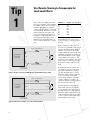
10
Practical
you need to
tips
know
about your
power
products
Simple ways to improve
your operation and
measurement capabilities
Use Remote Sensing to Compensate for
Load-Lead Effects
Tip
1
I3
When your power supply leaves the
factory, its regulation sense terminals
are usually connected to the output
terminals. This limits the supply’s
voltage regulation abilities, even with
very short leads. The longer the leads
and the higher the wire gauge, the
worse the regulation gets (Figure 1).
Compare the output impedance of a
well-regulated 10 A supply, which
might have an output impedance of
0.2 mΩ, with the resistance of copper
wire:
+
+S
5V
Load
4.7 V
–S
–
0.015 Ω lead resistance
Load leads are
6 foot, AWG 14
0.015 Ω lead resistance
+
16.1
10.2
6.39
4.02
2.53
1.59
0.999
And regulation gets even worse if
you use a relay to connect power to
the load.
Remote sensing, in which you connect the sense terminals of the power
supply’s internal feedback amplifier
directly to the load, lets the power
supply regulate its output at the load
terminals, rather than at its own output terminals (Figure 2). The supply
voltage shifts as necessary to compensate for the resistance of the load
leads, relays, or connectors, thereby
keeping the voltage at the load constant.
+S
5.3 V
–S
–
I2
0.015 Ω lead resistance
Load leads are
6 foot, AWG 14
Figure 2: Using remote sensing to correct the lead-load problem
2
22
20
18
16
14
12
10
To implement remote sensing, disconnect the local sense leads from
the output terminals. Use twisted
two-wire shielded cable to connect
the power supply sensing terminals
to the sense points on the load.
(Don’t use the shield as one of the
sensing conductors.) Connect one
end of the shield to ground and leave
the other end unconnected.
Figure 1: The effects of six feet of AWG 14-gauge leads without remote sensing
Power Supply
Programmed
for 5 V, 10 A
Resistance in mΩ/ft (at 20° C)
T3
0.015 Ω lead resistance
Power Supply
Programmed
for 5 V, 10 A
AWG wire size
Load
5V
Sensing currents are typically less
than 10 mA, and as a general rule,
you should keep the voltage drop in
the sense leads to less than 20 times
the power supply temperature coefficient (usually stated in mV/°C). This
is easy to achieve with readily available shielded two-wire cable.
Charge and Discharge Batteries in Less Time
Tip
2
Using a power supply in constantcurrent mode (Figure 1) is a simple
way to recharge batteries, and it also
lets you achieve 100% charge levels.
On the downside, this method is slow,
taking as long as 14-16 hours because
the charging current is only a fraction
of the battery’s amp/hour rating.
Pulse charging, also called transient
mode, shortens the charging time, yet
still charges the battery to over 90%
capacity (Figure 2). The electronic
load acts as a switch, providing the
current pulses. (Note that you can
also use an electronic load to program
constant-current charging.) Figure 3
shows a typical pulse-charging current
waveform.
To simulate battery drain, you can
also program the electronic load to
discharge batteries with either constant or pulse current waveforms. In
some cases, pulse discharging does
a better job of mimicking a product’s
energy-saving features. Simulating
cellular phone battery discharge,
for instance, is complex due to the
phone’s various operating modes—
standby, dialing, and talking. You can
create the necessary tri-level discharge
current wave-form shown in Figure 4
using the electronic load.
I
I2
I1
T
Figure 1: Constant current charging is simple and effective, but
it can be very slow. (The diode prevents the battery from discharging through the power supply if the supply voltage drops
below the battery voltage.)
I
I2
T1
Figure 2: Pulse charging using an electronic load is much
faster, while still achieving 90% recharge.
T
Figure 3: A typical pulse charging waveform created with an
electronic load
I1
T4
T3
T1
T2
T
Figure 4: A complex waveform that simulates the energy-saving
features in portable, battery-powered products
3
Tip
3
Increase Safety with Remote Disable
Feature
Remote disable offers a safe way to
shut down a power supply to respond
to some particular operating condition or to protect system operators
(in response to a cabinet door being
opened unexpectedly or someone
pushing a panic button, for instance).
Remote inhibit (RI) is an input to the
power supply that disables the output
when the RI terminal is pulled low
(Figure 1). Shorting the normally open
switch turns off the supply’s output.
You could also use a logic chip with
an open collector transistor output
instead of the switch. Figure 1 also
shows the discrete fault indicator
(DFI), which you can use to signal
an operator or other components in
the system whenever the power supply detects a user-defined fault.
Figure 1. Remote inhibit and discrete fault
indicator schematic
Figure 2. Daisy-chained DFI and RI
4
Almost any operating condition can
create a DFI signal. For example, to
generate a DFI signal when the load
draws excessive current, enable the
over current protection (OCP) mode,
program the unit to generate a DFI
signal when it enters constant current
mode, then program the maximum
current the load normally draws. If
the load current exceeds the maximum,
the DFI output goes low, disables the
power supply, and informs the operator of the over-current condition (or
performs another user-defined function), without tying up the system bus
or interrupting the system controller.
You can daisy chain DFI and RI as
shown in Figure 2. If one supply
detects a fault, all supplies in the
system are disabled. Using this
approach, you can chain together
an unlimited number of supplies.
Tip
4
Eliminate Noise from Low-Level
Measurements
Noise in low-level measurements
can come from a number of different
sources, and it’s easier to eliminate
noise than to filter it. Check these
noise sources:
1. Power Supply
Starting with a low-noise supply is
naturally a great way to keep noise
out of your measurements. Linear
power supplies have lower commonmode noise currents, and generally
operate at low frequency. However,
you can use switch-mode supplies
successfully if their specifications
include a low common-mode current.
As a rule of thumb, common-mode
current over 20-30 mA is likely to
cause trouble. Keep reading for hints
on how to minimize the problem.
2. DUT to Power Supply
Connections
Minimize conducted noise by eliminating ground loops. Ideally, there should
be only one connection to ground. In
rack systems, where multiple ground
points are inevitable, separate the dc
distribution path from other conductive paths that carry ground currents.
If necessary, float the power supply
(don’t connect either terminal directly
to ground).
Minimize radiated pick-up (both electric and magnetic) by using twisted
shielded conductors for the output
and remote sense leads. To make sure
the shield doesn’t carry current, connect the shield to ground at one end
only, preferably the single-point
ground on the supply (Figure 1).
Minimize the power supply’s commonmode noise current by equalizing the
impedance to ground from the plus
and minus output terminals. Also
equalize the DUT’s impedance to
ground from the plus and minus
input terminals. Magnetic coupling
or capacitive leakage provide a return
path for noisy ground loop current at
higher frequencies. To balance the
DUT’s impedance to ground for your
test frequencies, use a common-mode
choke in series with the output leads
and a shunt capacitor from each lead
to ground.
Figure 1: Minimizing radiated pick-up with twisted shield leads for both output and
remote sense leads
3. Current Variations to the DUT
Rapid changes in the DUT’s current
demand cause voltage spikes. To prevent this, add a bypass capacitor close
to the load. The capacitor should have
a low impedance at the highest testing
frequencies. Avoid imbalances in load
lead inductance; direct connections to
the DUT, such as twisted shielded
pair, are your best bet.
5
Tip
5
Use Down Programming to Increase Test
Speed
Under light or no load conditions, a
power supply’s output capacitor discharges slowly. If you’re using the
supply as a static voltage source, this
is not problematic, but when you’re
making tests at varying voltage levels,
slow discharge means slow tests.
Down programming circuits in power
supplies rapidly decrease the output
voltage, reducing discharge times by
hundreds of milliseconds. Agilent
Technologies power supplies use two
types of down programming circuits:
Figure 1: A down programming circuit
with an FET across the output terminals
Figure 2: A down programmer situated
between power supply’s positive output
and a negative source
6
• In Figure 1, an FET is placed
across the output terminals.
Whenever the output voltage is
higher than the programmed value,
the FET activates and discharges
the output capacitor. The FET can
sink currents ranging from 10% to
20% of the supply’s output current
rating. The maximum load at low
voltages is limited to the On resistance of the FET plus the series
monitoring resistor, resulting in a
slight degradation of the down
programming current near zero
volts.
• In Figure 2, the down programmer
lies between the power supply’s
positive terminal and a negative
source. This configuration pulls
the output completely down with
no degradation near zero.
Some power supplies, such as the
Agilent 662xA and 663xB series, can
sink currents equal to their full output current rating. In the 663xB
series, this sink current is programmable, so you can use the supply both
as a programmable source and load—
very useful in applications such as
charging and discharging batteries.
Ensure Proper Power-up with Foldback
Supplies
Tip
6
Foldback power supplies protect connected equipment by reducing excess
current (and thus output voltage)
along a foldback path. When testing
foldback power supplies using an
electronic load, you need to take
steps to be sure the power supply
starts properly.
Resistive Load
R1
V
R2
(R2 < R1)
Foldback
Region
I
Figure 1: Foldback behavior in constant
resistance mode
Constant Current Load
I1
V
P1
P2
When using an electronic load in
constant resistance mode, the current increases as the resistance
decreases, R1 to R2, until the current
limit is reached; after that, the supply
reduces its output current along the
foldback path (Figure 1).
To alleviate this problem, program
the electronic load to a value below
the current limit foldback point (Imin).
This value can be close to zero on
many supplies. After applying power
to the source, increase the load’s current limit to the desired value.
For power supplies that don’t require
a minimum load current at all times,
you can initially program the load
in constant resistance mode. Then,
when the power supply reaches its
nominal operating voltage, switch the
electronic load to constant current
mode. (During the transition, the
load momentarily goes to zero.)
For constant current load, the power
supply operates in constant voltage
mode while the electronic load operates in constant current mode. When
the power supply starts up, its output
voltage is zero, and the electronic
load tries to satisfy the programmed
current value (I1) by decreasing the
load resistance. The power supply
interprets the low load value as
an over-current condition, and
immediately folds back to a stable
operating point (P2 or P3 in Figure 2,
depending on the power supply’s
startup characteristics).
Foldback
Region
P3
Imin
I
Figure 2: Foldback behavior for constant
current load
7
R
Tip
7
Connect Power Supplies in Series or
Parallel for Higher Output
Connecting two or more power supplies in series (Figure 1) provides
higher voltages, but observe these
precautions:
Connecting two or more power supplies in parallel (Figure 2) provides
higher currents, but again, observe
these precautions:
• Never exceed the floating voltage
rating of any of the supplies.
• Never subject any of the power
supplies to negative voltages.
• One unit must operate in constant
voltage (CV) mode and the other(s)
in constant current (CC) mode.
• The output load must draw enough
current to keep the CC unit(s) in
CC mode.
Program each power supply independently. If two supplies are used, program each one for 50% of the total
output voltage. If three supplies are
used, program each supply for about
33% of the total output voltage. Set
the current limit of each supply to the
maximum that the load can safely
handle.
Figure 1: Connecting units in series
Figure 2: Connecting units in parallel
8
Program the current limit of each
unit to its maximum value and program the output voltage of the CV
unit to a value slightly lower than the
CC unit(s). The CC units supply the
maximum output current that they
have been set to and drop their output voltage until it matches the voltage of the CV unit, which supplies
only enough current to fulfill the total
load demand.
Tip
8
Use Your Power Supply to Measure Pulsed
Current
As a simpler and cheaper alternative,
use a power supply with built-in measurement capabilities. The Agilent
66312A and 66332A dynamic measurement dc sources store up to 4,096
data points at sample intervals from
15.6 ms to 31,200 s. Like an oscilloscope, they acquire pre- and postYou could use an oscilloscope to mon- trigger buffer data by crossing a
user-set threshold. These dynamic
itor a shunt or a current probe, but
this approach raises issues with volt- measurement capabilities are illustrated in an Agilent VEE program
age drops, ground loops, common
output panel (Figure 1).
mode noise, space, and calibration.
To adequately specify the power
source for products that exhibit
pulsed and dynamic current loading
(such as digital cellular phones and
hard drives), you need to evaluate
both the peak and dc averages current draws.
In Figure 2, note the SCPI commands
in the “Set Up Source,” “Measure,”
and “Enter Array” blocks. (You can
use these commands in other programming environments as well.)
Note that “MEAS” can be used in
place of “FETC” to cause an immediate trigger. Obtain subsequent measurement parameters from the same
data by using “FETC.”
Figure 1. An Agilent VEE program that makes parametric measurements and captures the pulse current
loading of a digital cellular phone
Figure 2. Block flow diagram of the Agilent VEE program, showing program details
9
Tip
9
Characterize Inrush Current with an AC
Power Source/Analyzer
The inrush current characteristics of
ac-dc switch mode power supplies
vary with the turn-on phase of the
voltage cycle. Usually, these power
supplies have input capacitors that
draw high peaks of inrush current as
they charge from the rectified ac line
at turn-on. Characterizing inrush current versus turn-on phase can provide some important design insights:
Output
Voltage
Start up
phase of
40 degrees
Bus Trigger
Inrush Current
Peak Current Measurement
Digitized Inrush
Current
Data Points
Figure 1: An inrush current measurement at 40° using Agilent 6800 series ac power
source/analyzers
10
• Uncover component stresses
• Check to see if a product produces
ac mains disturbances that interact with other products connected
to the same branch circuit
• Select proper fuses and circuit
breakers
However, this can be a challenging
measurement because you have to
synchronize the current digitization
and peak current measurement with
the startup phase of the voltage.
Worst case inrush currents occur
near the voltage cycle’s peak and
when the ac input capacitor of the
DUT is fully discharged at startup.
Therefore, you must perform tests at
incremental voltage startup phases
from around 40° to 90° (Figure 1)
and let the DUT’s ac input capacitor
discharge between tests.
A traditional test setup includes an
ac source with programmable phase
capability and an output trigger port,
a digital oscilloscope, and a current
probe. However, using an advanced
ac power source/analyzer such as the
Agilent 6800 series ac power
source/analyzers is easier because
they have built-in generation, current
waveform digitization, peak current
measurement, and synchronization
capabilities that let you perform
inrush current characterization without cabling and synchronizing separate instruments.
Tip
10
Use a Power Supply to Measure DUT
Supply Current
Accurately measuring DUT supply
currents above 10 A is beyond the
range of the typical DMM in ammeter
mode. You could use an external
shunt and the DMM’s voltage mode,
but using the power supply itself is a
better solution. Many supplies
include an accurate measurement
system, including a shunt. Using the
power source’s shunt to take current
or voltage measurements at the DUT
can be as simple as sending a MEAS
command.
The following table shows the level of
measurement accuracy you can
expect with a good-quality supply:
Output level
Typical accuracy
Full
10% of full output
1% of full output
0.1% to 0.5%
0.5% to 1%
near 10%
While the advantages of using the
power source to measure high currents is clear, using it to measure low
currents may not be as obvious. A
system DMM has 0.01% to 0.1% accuracy, although this doesn’t include
other possible errors that can affect
the measurement, such as cabling. In
contrast, the power supply accuracy
figures in the table include all applicable factors.
A good system DMM can measure
current down to the picoamp level,
but you rarely need to measure DUT
supply currents this low. In most
cases, the toughest measurement will
involve current draw by a batterypowered device in sleep mode (such
as a cellular phone), where measuring
1-10 mA with reasonable accuracy is
usually all you need.
Most power supplies’ current readback performs well between full scale
and 10% of full scale. Newer power
sources, such as the Agilent 66000A
modular power system, offer full
scale accuracy of 0.06% at 16 A and
3.8% accuracy at 160 mA. You can
also choose a power supply with multiple range readback. The 663XA
series can measure as low as 2.5 µA
and offers accuracy of 5.1% at 50 µA
(with full-scale accuracy of 0.2%).
Also, keep in mind that while ac
sources offer many current measurement options, including rms, newer
dc sources, such as the 66312A and
66332A, provide rms peak measurements as well (see Tip 8).
11
Power
products
that do more and
less
demand
Agilent Technologies’ “one-box” philosophy means we pack more and more capability into the power products
themselves, in some cases giving you a rack’s worth of capability in a single box. By offering more, these products
demand less from you—fewer instruments, less rack space, simpler test setups, and lower cost of ownership.
Dynamic measurement dc supplies
Solar array simulator
Autoranging dc supplies
The Agilent 66312A and 66332A are
the first power supplies with instantaneous peak measurement capability, so you no longer need a scope or
high-speed digital voltmeter to test
devices that draw pulsed current.
The Agilent E4350A solar array simulator mimics the output characteristics of a satellite’s solar panels. It’s
also a great example of our ability to
create unique power solutions to
meet unique application challenges.
The Agilent 6030-series autoranging
supplies are a flexible, convenient
solution when you need to test a wide
range of devices with a single supply
or test devices with a variety of operating points.
• Precision current measurement—as
low as 0.6 µA
• Dynamic voltage measurements
accurate to 0.03% + 5 mV
• Dynamic current measurements
accurate to 0.6% + 1 mA (66312A)
• Simulate I-V curves of a solar
array under various conditions
• Operate the system in three different modes for maximum flexibility
• Available as individual power
modules or as a turnkey system
customized to your needs
• Choose from six models with
power ratings from 200 W to 1 kW
• All models offer Agilent’s one-box
solution with built-in readback
• Current ranges from 2 to 120 A;
voltage ranges from 6.7 to 500 V
Dynamic measurement dc supplies
Model
Voltage
Current
Maximum power
66312A
66332A
0 to 20 V
0 to 2 A
40W
0 to 20 V
0 to 5 A
100W
Solar array simulator
Model
Voltage
Current
Maximum power
E4350A
0 to 60 V
0 to 8 A
450W
Auto-ranging supplies
Model
6033A
6038A
6030A
6031A
6032A
6035A
Voltage
Current
Maximum output power at any
valid combination of V and I
0 to 20 V
0 to 30 A
0 to 60 V
0 to 10 A
0 to 200 V
0 to 17 A
0 to 20 V
0 to 120 A
0 to 60 V
0 to 50 A
0 to 500 V
0 to 5 A
200 W
200 W
1000 W
1000 W
1000 W
1000 W
12
Power you can count on year after year
We’ve been a leader in the power
products business for more than
three decades because engineers like
you know they can count on Agilent
performance, reliability and value.
Even our least-expensive dc supplies
offer low ripple and noise with tight
load and line regulation. Our highprecision products give you the
exact power levels you need, with
accurate readback measurements
to match. Plus, every product you
see here is covered by a three-year
warranty.
Single-output dc supplies
These supplies will clean up your
ATE power without cleaning out your
budget. Not only do you buy more
performance with the Agilent 6600series, their one-box integration
means you’ll buy less equipment
overall, too.
To learn more about these power
solutions, please use the reply card
or visit our Web site at
www.agilent.com/find/power.
For immediate service, call one of
the engineers at Agilent at 800-4524844.
• Clean, reliable dc power from 40 W
to 5 kW
• Designed for fast, easy system
integration
• Built-in V & I readback for one-box
convenience
Single-output dc supplies
40 W and 100 W
Voltage
Current
200 W
Output voltage
Output current (40° C)
Maximum current (50° C)
Maximum current (55° C)
500 W
Output voltage
Ouput current (40° C)
Maximum current (50° C)
Maximum current (55° C)
2 kW
Output voltage
Output current
5 kW
Voltage
Current (derated linearly
1%/° C to 55° C)
* Economy versions with identical specifications, but without GPIB.
6612B
6632B
6633B
6634B
0 to 20 V
0 to 2 A
0 to 20 V
0 to 5 A
0 to 50 V
0 to 2 A
0 to 100 V
0 to 1 A
6541A*
6641A
6542A*
6642A
6543A*
6643A
6544A*
6644A
6545A*
6645A
0 to 8 V
0 to 20 A
18.0 A
17.0 A
0 to 20 V
0 to 10 A
9.0 A
8.5 A
0 to 35 V
0 to 6 A
5.4 A
5.1 A
0 to 60 V
0 to 3.5 A
3.2 A
3.0 A
0 to 120 V
0 to 1.5 A
1.4 A
1.3 A
6551A*
6651A
6552A*
6652A
6553A*
6653A
6554A*
6654A
6555A*
6655A
0 to 8 V
0 to 50 A
45.0 A
42.5 A
0 to 20 V
0 to 25 A
22.5 A
21.3 A
0 to 35 V
0 to 15 A
13.5 A
12.8 A
0 to 60 V
0 to 9 A
8.1 A
7.7 A
0 to 120 V
0 to 4 A
3.6 A
3.4 A
6571A*
6671A
6572A*
6672A
6573A*
6673A
6574A*
6674A
6575A*
6675A
0 to 8 V
0 to 220 A
0 to 20 V
0 to 100 A
0 to 35 V
0 to 60 A
0 to 60 V
0 to 35 A
0 to 120 V
0 to 18 A
6680A
6681A
6682A
6683A
6684A
0 to 5 V
0 to 8 V
0 to 21 V
0 to 32 V
0 to 40 V
0 to 875 A
0 to 580 A
0 to 240 A
0 to 160 A
0 to 128 A
13
Power products that do more and demand less
Multiple-output dc supplies
Modular power system
Electronic Loads
The Agilent 6620-series’ multiple outputs and integrated I & V readback
dramatically simplify the job of system integration and maintenance.
Plus, the 6625A, 6626A, 6628A and
6629A models offer the precision of
14-bit dual range programming and
readback.
With rack space at a premium, the
Agilent 66000 modular power system’s
growing popularity is no surprise. A
single mainframe can hold up to eight
modules, and you can choose from six
modules with voltage ranges up to
200 V and current ranges up to 16 A.
Agilent’s integrated electronic loads
help you save time, money, and rack
space while delivering precise control
and all the capabilities you need for
analyzing dc power sources and
devices. Use the programable pulse
waveform generator or use analog
programming to simulate real-life
load conditions.
• Choose 2, 3, or 4 independent, isolated outputs
• Precision programming and readback
• Built-in readback for one-box convenience and value
• High power density—up to eight
supplies in seven inches of rack
space
• Low noise, stable power
• High accuracy programming and
readback
• Ideal for evaluating dc power
sources and power components
• Lower costs while improving ease
of use and test quality
• Single-input and modular units
with proven record of reliability
Multiple-output dc supplies
Model
40-W output
Low-range volts, amps
0 to 7 V, 0 to 5 A
High-range volts, amps
0 to 20 V, 0 to 2 A
Output combinations for each model (total number of outputs)
6621A (2)
—
6622A (2)
—
6623A (3)
1
6624A (4)
2
6627A (4)
—
40-W output
0 to 20 V, 0 to 2 A
0 to 50 V, 0 to 0.8 A
80-W output
0 to 7 V, 0 to 10 A
0 to 20 V, 0 to 4 A
80-W output
0 to 20 V, 0 to 4 A
0 to 50 V, 0 to 2A
—
—
1
2
4
2
—
1
—
—
—
2
—
—
—
High range
0 to 50 V
0 to 500 mA
Low range
0 to 16 V
0 to 200 mA
Precision multiple-output supplies
Model
Output power
25-W output
Output range
Low range
Output volts
0 to 7 V
Output amps
0 to 15 mA
Output combinations for each model (total number of outputs)
6625A (2)
6626A (4)
6628A (2)
6629A (4)
50-W output
1
2
0
0
High range
0 to 50 V or 0 to 16 V
0 to 1 A or 0 to 2 A
1
2
2
4
Modular power systems
Model
Output ratings at 40° C
Output voltage
Output current
Maximum power
66101A
66102A
66103A
66104A
66105A
66106A
0 to 8 V
0 to 16 A
128 W
0 to 20 V
0 to 7.5 A
150 W
0 to 35 V
0 to 4.5 A
157.5 W
0 to 60 V
0 to 2.5 A
150 W
0 to 120 V
0 to 1.25 A
150 W
0 to 200 V
0 to 0.75 A
150 W
6060B, 60502B
3-60 V
300 W
6063B, 60503B
3-240 V
250 W
60501B
3-60 V
150 W
60504B
3-150 V
600W
60507
3-150 V
500 W
Electronic Loads
Model
Input voltage
Maximum power
14
AC power source/analyzers
From avionics to uninterruptible
power supplies, customers are
demanding products that can use
power efficiently while handling all
kinds of ac line disturbances. To
make sure your products meet these
growing expectations, test them with
the Agilent 6800-series ac power
source/analyzers.
• The fast, easy way to generate both
clean and distorted ac power for
product testing
• A complete solution in a single,
compact, tightly integrated box
with graphical user interface
• Built-in 16-bit power analyzer precisely measures all important
parameters
Harmonic/flicker test systems
The Agilent 6840-series harmonic/
flicker test systems transform an
expensive headache into a competitive advantage. Instead of sending
prototypes out to a test lab and waiting for the results, you can now
afford to do your own compliance
testing—whenever and wherever you
need.
• Compliance-level testing of IEC
low-frequency emission standards
• An inexpensive, integrated solution that is easier to install, use,
and maintain
• Advanced diagnostics go beyond
simple pass/fail to help you modify
designs quickly
We’ve combined a precision ac source
with built-in power analysis, flickermeter, complete testing and reporting
software, and our in-depth knowledge
of the IEC standards. The result is
much less expensive and easier to
maintain than traditional testers built
from separate instruments.
The 6840 test system is easy to set up
and the graphical software is easy to
use, so you don’t need to be a compliance expert to get dependable results.
You’ll have both real-time and off-line
data analysis and review, plus report
generation and data archiving for
thorough test documentation.
AC Power Source/analyzers
Model
Max power
# of phases
6811A
6812A
6813A
6814B
6834B
375 VA
1
750 VA
1
1750 VA
1
3000 VA
1
4500 VA
1/3
6841A
6842A
6843A
750 VA
1
1750 VA
1
4800 VA
1
Harmonic flicker test systems
Model
Max power
# of phases
For more information, please use the reply card inside, visit our Web site at www.agilent.com/find/power, or call Agilent
at 800-452-4844.
15
You’re trying to get the most from
your power products and get the best
power products for your money—-and
this booklet is a great place to start.
You’ll find 10 easy and practical ways
to improve power generation and
measurement, along with a brief look
at our most popular power instruments and systems.
For more information, please use the
reply card inside, visit our website at
www.agilent.com/find/power, or call
Agilent at 800-452-4844.
Agilent Technologies’ Test and Measurement
Support, Services, and Assistance
Agilent Technologies aims to maximize
the value you receive, while minimizing
your risk and problems. We strive to
ensure that you get the test and measurement capabilities you paid for and obtain
the support you need. Our extensive support resources and services can help you
choose the right Agilent products for your
applications and apply them successfully.
Every instrument and system we sell has
a global warranty. Support is available
for at least five years beyond the production life of the product. Two concepts
underlie Agilent’s overall support policy:
“Our Promise” and “Your Advantage.”
Our Promise
“Our Promise” means your Agilent test
and measurement equipment will meet its
advertised performance and functionality.
When you are choosing new equipment,
we will help you with product information, including realistic performance specifications and practical recommendations
from experienced test engineers. When
you use Agilent equipment, we can verify
that it works properly, help with product
operation, and provide basic measurement
assistance for the use of specified capabilities, at no extra cost upon request. Many
self-help tools are available.
Your Advantage
“Your Advantage” means that Agilent
offers a wide range of additional expert
test and measurement services, which you
can purchase according to your unique
technical and business needs. Solve problems efficiently and gain a competitive edge
by contracting with us for calibration, extracost upgrades, out-of-warranty repairs, and
on-site education and training, as well
as design, system integration, project management, and other professional services.
Experienced Agilent engineers and technicians worldwide can help you maximize
your productivity, optimize the return on
investment of your Agilent instruments and
systems, and obtain dependable measurement accuracy for the life of those products.
Get assistance with all your
test and measurement needs at:
www.agilent.com/find/assist
Product specifications and descriptions in
this document subject to change without notice.
Copyright © 1997, 2000 Agilent Technologies
Printed in U.S.A. 8/00
5965-8239E