Download Agilent Technologies 86100C Specifications

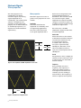
Agilent Technologies
Oscilloscope Fundamentals
Application Note 1606
This application note provides an overview of oscilloscope fundamentals. You will
learn what an oscilloscope is and how it operates. We will discuss oscilloscope
applications and give you an overview of basic measurements and performance
characteristics. We will also take a look at the different types of probes and
discuss their advantages and disadvantages.
Introduction
Table of Contents
Introduction . . . . . . . . . . . . . . . . . . . . . . 1
Electronic Signals . . . . . . . . . . . . . . . . . 2
Wave properties . . . . . . . . . . . . . . . . . . . . 2
Waveforms . . . . . . . . . . . . . . . . . . . . . . . . 3
Analog versus digital signals . . . . . . . . . . 4
What is an Oscilloscope and
Why Do You Need One? . . . . . . . . . . . . 5
Signal integrity . . . . . . . . . . . . . . . . . . . . . 5
What an oscilloscope looks like . . . . . . . 6
An oscilloscope’s purpose . . . . . . . . . . . . 7
Types of oscilloscopes . . . . . . . . . . . . . . . 8
Where oscilloscopes are used . . . . . . . . 10
Basic Oscilloscope Controls and
Measurements . . . . . . . . . . . . . . . . . . . 11
Basic front-panel controls . . . . . . . . . . .
Softkeys . . . . . . . . . . . . . . . . . . . . . . . . . .
Basic measurements . . . . . . . . . . . . . . .
Basic mathematical functions . . . . . . . .
11
14
15
16
Important Oscilloscope
Performance Characteristics . . . . . . . 17
Bandwidth . . . . . . . . . . . . . . . . . . . . . . . .
Channels . . . . . . . . . . . . . . . . . . . . . . . . .
Sample rate . . . . . . . . . . . . . . . . . . . . . . .
Memory depth . . . . . . . . . . . . . . . . . . . . .
Update rate . . . . . . . . . . . . . . . . . . . . . . .
Oscilloscope connectivity . . . . . . . . . . .
17
17
18
19
20
20
Oscilloscope Probes . . . . . . . . . . . . . . 21
Loading . . . . . . . . . . . . . . . . . . . . . . . . . .
Passive probes . . . . . . . . . . . . . . . . . . . .
Active probes . . . . . . . . . . . . . . . . . . . . .
Current probes . . . . . . . . . . . . . . . . . . . .
Probe accessories . . . . . . . . . . . . . . . . .
21
21
21
22
22
Conclusion . . . . . . . . . . . . . . . . . . . . . . 23
Sales and Service . . . . . . . . . . . . . . . . 24
Electronic technology permeates
our lives. Millions of people
use electronic devices such as
cell phones, televisions, and
computers on a daily basis.
As electronic technology
has advanced, the speeds at
which these devices operate
have accelerated. Today, most
devices use high-speed digital
technologies.
Engineers need the ability
to accurately design and test
the components in their highspeed digital devices. The
instrumentation engineers use to
design and test their components
must be particularly well-suited
to deal with high speeds and
high frequencies. An oscilloscope
is an example of just such an
instrument.
Oscilloscopes are powerful tools
that are useful for designing
and testing electronic devices.
They are vital in determining
which components of a system
are behaving correctly and
which are malfunctioning. They
can also help you determine
whether or not a newly designed
component behaves the way you
intended. Oscilloscopes are far
more powerful than multimeters
because they allow you to see
what the electronic signals
actually look like.
Oscilloscopes are used in a
wide range of fields, from the
automotive industry to university
research laboratories to the
aerospace-defense industry.
Companies rely on oscilloscopes
to help them uncover defects and
produce fully functional products.
Oscilloscopes are essential
to meeting the needs of their
customers with new and better
electronic products.
Electronic Signals
Wave properties
The main purpose of an
oscilloscope is to display
electronic signals. By viewing
signals displayed on an
oscilloscope, you can determine
whether a component of an
electronic system is behaving
properly. So, to understand how
an oscilloscope operates, it is
important to understand basic
signal theory.
Wave properties
Electronic signals are waves or
pulses. Basic properties of waves
include:
Amplitude
Two main definitions for
amplitude are commonly used
in engineering applications.
The first is often referred to
as the peak amplitude and is
peak amplitude
RMS amplitude
defined as the magnitude of the
maximum displacement of a
disturbance. The second is called
the root-mean-square (RMS)
amplitude. To calculate the RMS
voltage of a waveform, square the
waveform, find its average voltage
and take the square root.
For a sine wave, the RMS
amplitude is equal to 0.707 times
the peak amplitude.
Phase shift
Phase shift refers to the amount
of horizontal translation between
two otherwise identical waves.
It is measured in degrees
or radians. For a sine wave,
one cycle is represented by
360 degrees. Therefore, if two
sine waves differ by half of a
cycle, their relative phase shift is
180 degrees.
Period
The period of a wave is simply the
amount of time it takes for a wave
to repeat itself. It is measured in
units of seconds.
Figure 1. Peak amplitude and RMS amplitude for a sine wave
period
Figure 2. The period of a triangular wave
Oscilloscope Fundamentals
Frequency
Every periodic wave has a
frequency. The frequency is
simply the number of times a
wave repeats itself within one
second (if you are working in
units of Hertz). The frequency is
also the reciprocal of the period.
Electronic Signals (continued)
Waveforms
Waveforms
A waveform is the shape or
representation of a wave.
Waveforms can provide you with
a great deal of information about
your signal. For example, it can
tell you if the voltage changes
suddenly, varies linearly, or
remains constant. There are many
standard waveforms, but this
section will cover the ones you
will encounter most frequently.
Sine waves
Sine waves are typically
associated with alternating
current (AC) sources such as an
electrical outlet in your house. A
sine wave does not always have
a constant peak amplitude. If
the peak amplitude continually
decreases as time progresses, we
call the waveform a damped sine
wave.
Square/rectangular waves
A square waveform periodically
jumps between two different
values such that the lengths
of the high and low segments
are equivalent. A rectangular
waveform differs in that the
lengths of the high and low
segments are not equal.
Figure 3. A sine wave
Figure 4. A square wave
Oscilloscope Fundamentals
Electronic Signals (continued)
Waveforms
Triangular/sawtooth waves
In a triangular wave, the voltage
varies linearly with time. The
edges are called ramps because
the waveform is either ramping
up or ramping down to certain
voltages. A sawtooth wave looks
similar in that either the front
or back edge has a linear voltage
response with time. However,
the opposite edge has an almost
immediate drop.
Pulses
A pulse is a sudden single
disturbance in an otherwise
constant voltage. Imagine flipping
the switch to turn the lights on in
a room and then quickly turning
them off. A series of pulses is
called a pulse train. To continue
our analogy, this would be like
quickly turning the lights on and
off over and over again.
Pulses are the common waveform
of glitches or errors in your
signal. A pulse might also be the
waveform if the signal is carrying
a single piece of information.
Analog versus digital signals
Analog signals are able to take on
any value within some range. It is
useful to think of an analog clock.
The clock hands spin around the
clock face every twelve hours.
During this time, the clock
hands move continuously. There
are no jumps or discreteness
in the reading. Now, compare
this to a digital clock. A digital
clock simply tells you the hour
and the minute. It is, therefore,
discretized into minute intervals.
One second it might be 11:54 and
then it jumps to 11:55 suddenly.
Digital signals are likewise
discrete and quantized. Typically,
discrete signals have two possible
values (high or low, 1 or 0, etc.).
The signals, therefore, jump back
and forth between these two
possibilities.
Figure 5. A triangular wave
Complex waves
Waves can also be mixtures of the
above waveforms. They do not
necessarily need to be periodic
and can take on very complex
waveforms.
Figure 6. A sawtooth wave
Figure 7. A pulse
Oscilloscope Fundamentals
What Is an Oscilloscope and Why Do You Need One?
Signal integrity
Signal integrity
The main purpose of an
oscilloscope is to give an
accurate visual representation
of electrical signals. For this
reason, signal integrity is very
important. Signal integrity refers
to the oscilloscope’s ability to
reconstruct the waveform so that
it is an accurate representation
of the original signal. An
oscilloscope with low signal
integrity is useless because it is
pointless to perform a test when
the waveform on the oscilloscope
does not have the same shape
or characteristics as the true
signal. It is, however, important
to remember that the waveform
on an oscilloscope will never
be an exact representation of
the true signal, no matter how
good the oscilloscope is. This
is because when you connect
an oscilloscope to a circuit, the
oscilloscope becomes part of the
circuit. In other words, there are
some loading effects. Instrument
makers strive to minimize loading
effects, but they always exist to
some degree.
Oscilloscope Fundamentals
What Is an Oscilloscope and Why Do You Need One? (continued)
What an oscilloscope looks like
What an oscilloscope looks like
In general, modern digitizing
oscilloscopes look similar to the
one seen in Figure 8. However,
there are a wide variety of
oscilloscope types, and yours
may look very different. Despite
this, there are some basic
features that most oscilloscopes
have. The front panel of most
oscilloscopes can be divided
into several basic sections: the
channel inputs, the display, the
horizontal controls, the vertical
controls, and the trigger controls.
If your oscilloscope does not have
a Microsoft® Windows®-based
operating system, it will probably
have a set of softkeys to control
on-screen menus.
display is simply the screen
where these signals are displayed.
The horizontal and vertical
control sections have knobs
and buttons that control the
horizontal axis (which typically
represents time) and vertical axis
(which represents voltage) of the
signals on the screen display.
The trigger controls allow you to
tell the oscilloscope under what
conditions you want the timebase
to start a sweep.
Display
An example of what the back
panel of an oscilloscope looks like
is seen in Figure 9.
As you can see, many
oscilloscopes have the
connectivity features found on
personal computers. Examples
include CD-ROM drives, CD-RW
drives, DVD-RW drives, USB
ports, serial ports, and external
monitor, mouse, and keyboard
inputs.
Horizontal control section
You send your signals into the
oscilloscope via the channel
inputs, which are connectors
for plugging in your probes. The
Trigger
control
section
Vertical
control
section
Softkeys
Channel inputs
Figure 8. Front panel on the Agilent InfiniiVision 5000 Series oscilloscope
Figure 9. Rear panel on the Agilent
Infiniium 8000 Series oscilloscope
Oscilloscope Fundamentals
What Is an Oscilloscope and Why Do You Need One? (continued)
An oscilloscope’s purpose
An oscilloscope’s purpose
An oscilloscope is a measurement
and testing instrument used to
display a certain variable as a
function of another. For example,
it can plot on its display a graph
of voltage (y-axis) versus time
(x-axis). Figure 10 shows an
example of such a plot. This
is useful if you want to test a
certain electronic component
to see if it is behaving properly.
If you know what the waveform
of the signal should be after
exiting the component, you can
use an oscilloscope to see if the
component is indeed outputting
the correct signal. Notice also
that the x and y-axes are broken
into divisions by a graticule. The
graticulte enables you to make
measurements by hand, although
with modern oscilloscopes, most
of these measurements can be
made by the oscilloscope itself.
An oscilloscope can also do more
than plot voltage versus time.
An oscilloscope has multiple
inputs, called channels, and each
one of these acts independently.
Therefore, you could connect
channel 1 to a certain device
and channel 2 to another. The
oscilloscope could then plot the
voltage measured by channel 1
versus the voltage measured by
channel 2. This mode is called
the XY-mode of an oscilloscope.
It is useful when graphing I-V
plots or Lissajous patterns where
the shape of these patterns tells
you the phase difference and the
frequency ratio between the two
signals. Figure 11 shows examples
of Lissajous patterns and the
phase difference/frequency ratio
they represent.
Figure 10. An oscilloscope’s voltage versus time display of a
square wave
180 degrees; 1:1 ratio
90 degrees; 1:1 ratio
90 degrees; 1:2 ratio
30 degrees; 1:3 ratio
Figure 11. Lissajous patterns
Oscilloscope Fundamentals
What Is an Oscilloscope and Why Do You Need One? (continued)
Types of oscilloscopes
Types of oscilloscopes
Analog oscilloscopes
The first oscilloscopes were
analog oscilloscopes, which use
cathode-ray tubes to display a
waveform. An electron beam is
scanned across a series of many
horizontal lines while being gated
on and off. Photoluminescent
phosphor on the screen
illuminates when an electron
hits it, and as successive bits of
phosphor light up, you can see
a representation of the signal.
A trigger is needed to make
the displayed waveform look
stable. When one whole trace
of the display is completed, the
oscilloscope waits until a specific
event occurs (for example, a
rising edge that crosses a certain
voltage) and then starts the trace
again. An untriggered display is
unusable because the waveform is
not shown as a stable waveform
on the display (this is true for
DSO and MSO oscilloscopes,
which will be discussed below,
as well).
Analog oscilloscopes are useful
because the illuminated phosphor
does not disappear immediately.
You can see several traces of
the oscilloscope overlapping
each other, which allows you to
see glitches or irregularities in
the signal. Since the display of
the waveform occurs when an
electron strikes the screen, the
intensity of the displayed signal
correlates to the intensity of the
actual signal. This makes the
display act as a three-dimensional
plot (in other words, x-axis is
time, y-axis is voltage, and z-axis
is intensity).
Digital storage oscilloscopes (DSOs)
Digital storage oscilloscopes
(often referred to as DSOs) were
invented to remedy many of
the negative aspects of analog
oscilloscopes. DSOs input a
signal and then digitize it through
the use of an analog-to-digital
converter. Figure 12 shows an
example of one DSO architecture
used by Agilent digital
oscilloscopes.
The downside of an analog
oscilloscope is that it cannot
“freeze” the display and keep the
waveform for an extended period
of time. Once the phosphorus
substance deluminates, that part
of the signal is lost. Also, you
cannot perform measurements
on the waveform automatically.
Instead you have to make
measurements by hand using
the grid on the display. Analog
oscilloscopes are also very
limited in the types of signals
they can display because there
is an upper limit to how fast the
horizontal and vertical sweeping
of the electron beam can occur.
While analog oscilloscopes are
still used by many people today,
they are not sold very often.
Instead, digital oscilloscopes are
the modern tool of choice.
The attenuator scales the
waveform. The vertical amplifier
provides additional scaling while
passing the waveform to the
analog-to-digital converter (ADC).
The ADC samples and digitizes
the incoming signal. It then stores
this data in memory. The trigger
looks for trigger events while
the time base adjusts the time
display for the oscilloscope. The
microprocessor system performs
any additional postprocessing
you have specified before the
signal is finally displayed on the
oscilloscope.
Channel
memory
Channel
Input
Attenuater
Vertical
amplifier
ADC
Trigger
Figure 12. Digitizing oscilloscope architecture
Oscilloscope Fundamentals
MegaZoom
Time-base
Microprocessor
Display
Having the data in digital
form enables the oscilloscope
to perform a variety of
measurements on the waveform.
Signals can also be stored
indefinitely in memory. The data
can be printed or transferred to a
computer via a flash drive, LAN,
or DVD-RW. In fact, software
now allows you to control and
monitor your oscilloscope from
a computer using a virtual front
panel.
What Is an Oscilloscope and Why Do You Need One? (continued)
Types of oscilloscopes
Mixed signal oscilloscopes (MSOs)
In a DSO, the input signal is
analog and the digital-to-analog
converter digitizes it. However,
as digital electronic technology
expanded, it became increasingly
necessary to monitor analog and
digital signals simultaneously.
As a result, oscilloscope vendors
began producing mixed-signal
oscilloscopes that can trigger
on and display both analog and
4 analog channels
digital signals. Typically there
are a small number of analog
channels (2 or 4) and a larger
number of digital channels (see
Figure 13).
Mixed-signal oscilloscopes have
the advantage of being able
to trigger on a combination of
analog and digital signals and
display them all, correlated on
the same time base.
16 digital
Figure 13. Front panel inputs for the four analog channels and 16
digital channels on a mixed-signal oscilloscope
Portable/handheld oscilloscopes
As its name implies, a portable
oscilloscope is one that is small
enough to carry around. If you
need to move your oscilloscope
around to many locations or
from bench to bench in your
lab, then a portable oscilloscope
may be perfect for you. Figure
14 shows an example of a
portable instrument, the Agilent
InfiniiVision 5000 Series
oscilloscope.
The advantages of portable
oscilloscopes are that they are
lightweight and portable, they
turn on and off quickly, and they
are easy to use. They tend to
not have as much performance
power as larger oscilloscopes,
but scopes like the Agilent
InfiniiVision 5000, 6000, and
7000 Series are changing that.
These oscilloscopes offer all the
portability and ease typically
found in portable oscilloscopes,
but are also powerful enough
to handle all of your debugging
needs.
Figure 14. Agilent InfiniiVision 5000 Series portable oscilloscope
Oscilloscope Fundamentals
What Is an Oscilloscope and Why Do You Need One? (continued)
Types of oscilloscopes
Economy oscilloscopes
Economy oscilloscopes are
reasonably priced, but they do
not have as much performance
capability as high-performance
oscilloscopes. These oscilloscopes
are typically found in university
laboratories. The main advantage
of these oscilloscopes is their
low price. For a relatively modest
amount of money, you get a very
useful oscilloscope.
High-performance oscilloscopes
High-performance oscilloscopes
provide the best performance
capabilities available. They are
used by people who require
high bandwidth, fast sampling
and update rates, large memory
depth, and a vast array of
measurement capabilities.
Figure 15 shows an example of
a high-performance oscilloscope,
the Agilent Infiniium 90000A
Series oscilloscope.
The main advantage of a
high‑performance oscilloscope
is that it enables you to properly
analyze a wide range of signals
and provides many applications
and tools that make analyzing
current technology simpler and
faster. The main disadvantage of
high-performance oscilloscopes is
their price and size.
Where oscilloscopes are used
If a company is testing or using
electronic signals, it is highly
likely they have an oscilloscope.
For this reason, oscilloscopes are
prevalent in a wide variety
of fields:
• Automotive technicians use
oscilloscopes to diagnose
electrical problems in cars.
• University labs use
oscilloscopes to teach students
about electronics.
• Research groups all over the
world have oscilloscopes at
their disposal.
• Cell phone manufacturers
use oscilloscopes to test the
integrity of their signals.
• The military and aviation
industries use oscilloscopes
to test radar communication
systems.
• R&D engineers use
oscilloscopes to test and design
new technologies.
• Oscilloscopes are also used for
compliance testing. Examples
include USB and HDMI where
the output must meet certain
standards.
This is just a small subset of the
possible uses of an oscilloscope.
It truly is a versatile and powerful
instrument.
Figure 15. Agilent Infiniium 90000A Series oscilloscope
10
Oscilloscope Fundamentals
Basic Oscilloscope Controls and Measurements
Basic front-panel controls
Basic front-panel controls
Typically, you operate an
oscilloscope using the knobs
and buttons on the front panel.
In addition to controls found
of the front panel, many highend oscilloscopes now come
equipped with operating systems,
and as a result, they behave like
computers. You can hook up
a mouse and keyboard to the
oscilloscope and use the mouse
to adjust the controls through
drop down menus and buttons on
the display as well. In addition,
some oscilloscopes have touch
screens so you can use a stylus or
fingertip to access the menus.
Before you begin . . .
When you first sit down at your
oscilloscope, check that the
input channel you are using is
turned on. Then press [Default
Settings] if there is one. This
will return the oscilloscope to
its original default state. Then
press [Autoscale] if there is one.
This will automatically set the
vertical and horizontal scale
such that your waveform can be
nicely viewed on the display. Use
this as a starting point and then
make needed adjustments. If you
ever lose track of your waveform
or you are having a hard time
displaying it, repeat these steps.
Most oscilloscope front panels
contain at least four main
sections: vertical and horizontal
controls, triggering controls and
input controls.
Vertical controls
Vertical controls on an
oscilloscope typically are grouped
in a section marked Vertical;
these controls allow you to
adjust the vertical aspects of
the display. For example, there
will be a control that designates
the number of volts per division
(scale) on the y-axis of the
display grid. You can zoom in on a
waveform by decreasing the volts
per division or you can zoom
out by increasing this quantity.
There also is a control for the
vertical offset of the waveform.
This control simply translates
the entire waveform up or down
on the display. You can see the
vertical control section for an
Agilent InfiniiVision 5000 Series
oscilloscope in Figure 16.
Turns channel 1 on
Horizontal controls
An oscilloscope's horizontal
controls typically are grouped
in a front-panel section marked
Horizontal. These controls enable
you to make adjustments to the
horizontal scale of the display.
There will be a control that
designates the time per division
on the x-axis. Again, decreasing
the time per division enables you
to zoom in on a narrower range of
time. There will also be a control
for the horizontal delay (offset).
This control enables you to scan
through a range of time. You can
see the horizontal control section
for the Agilent InfiniiVision 5000
Series oscilloscope in Figure 17.
Adjusts the vertical scaling for channel 4
Vertically translates the waveform on channel 3
Figure 16. Front panel vertical control section on an Agilent InfiniiVision
5000 Series oscilloscope
Adjusts the horizontal scaling
Horizontally translates the waveform
Figure 17. Front panel horizontal control section on an
Agilent InfiniiVision 5000 Series oscilloscope
Oscilloscope Fundamentals
11
Basic Oscilloscope Controls and Measurements (continued)
Basic front-panel controls
Trigger controls
As we mentioned earlier,
triggering on your signal helps to
provide a stable, usable display
and allows you to see the part of
the waveform you are interested
in. The trigger controls let you
pick your vertical trigger level
(for example, the voltage at which
you want your oscilloscope to
trigger) and choose between
various triggering capabilities.
Examples of common triggering
types include:
Trigger voltage
Rising edge triggering
Figure 18. When you trigger on a rising
edge, the oscilloscope triggers when the
trigger threshold is reached
Edge triggering – Edge triggering
is the most popular triggering
mode. The trigger occurs when
the voltage surpasses some set
threshold value. You can choose
between triggering on a rising or
a falling edge. Figure 18 shows
a graphical representation of
triggering on a rising edge.
Glitch triggering – Glitch triggering
mode enables you to trigger on
an event or pulse whose width
is greater than or less than
some specified length of time.
This capability is very useful for
finding random glitches or errors.
If these glitches do not occur very
often, it may be very difficult
to see them. However, glitch
triggering allows you to catch
many of these errors. Figure 19
shows a glitch caught by an
Agilent InfiniiVision 6000 Series
oscilloscope.
12
Oscilloscope Fundamentals
Figure 19. An infrequent glitch caught on an Agilent InfiniiVision
6000 Series oscilloscope
Basic Oscilloscope Controls and Measurements (continued)
Basic front-panel controls
Pulse-width triggering – Pulse
width triggering is similar to
glitch triggering when you are
looking for specific pulse widths.
However, it is more general in
that you can trigger on pulses of
any specified width and you can
choose the polarity (negative or
positive) of the pulses you want
to trigger on. You can also set
the horizontal position of the
trigger. This allows you to see
what occurred pre-trigger or
post-trigger. For instance, you
can execute a glitch trigger, find
the error, and then look at the
signal pre-trigger to see what
caused the glitch. If you have the
horizontal delay set to zero, your
trigger event will be placed in the
middle of the screen horizontally.
Events that occur right before
the trigger will be to the left of
the screen and events that occur
directly after the trigger will be
to the right of the screen. You
also can set the coupling of the
trigger and set the input source
you want to trigger on. You do not
always have to trigger on your
signal, but can instead trigger on
a related signal. Figure 20 shows
the trigger control section of an
oscilloscope’s front panel.
Input controls
There are typically two or
four analog channels on an
oscilloscope. They will be
numbered and they will also
usually have a button associated
with each particular channel
that enables you to turn them
on or off. There may also be
a selection that allows you to
specify AC or DC coupling. If DC
coupling is selected, the entire
signal will be input. On the other
hand, AC coupling blocks the
DC component and centers the
waveform about 0 volts (ground).
In addition, you can specify
the probe impedance for each
channel through a selection
button. The input controls also let
you choose the type of sampling.
There are two basic ways to
sample the signal:
Real-time sampling – Real-time
sampling samples the waveform
often enough that it captures a
complete image of the waveform
with each sweep. This is useful if
you are sampling low-frequency
signals, as the oscilloscope has
the required time to sample the
waveform often enough in one
sweep.
Equivalent-time sampling –
Equivalent time sampling builds
up the waveform over several
sweeps. It samples part of the
signal on the first sweep, then
another part on the second
sweep, and so on. It then laces
all this information together
to recreate the waveform.
Equivalent time sampling is
useful for high-frequency signals
that are too fast for real-time
sampling.
Adjusts the trigger level
These keys allow you to
select the trigger mode
Figure 20. Front panel trigger control section on an Agilent InfiniiVision 5000 Series oscilloscope
Oscilloscope Fundamentals
13
Basic Oscilloscope Controls and Measurements (continued)
Softkeys
Softkeys
Softkeys are found on
oscilloscopes that do not have
Windows-based operating
systems (refer to Figure 8 for
a picture of softkeys). These
softkeys allow you to navigate
the menu system on the
oscilloscope’s display. Figure 21
shows what a popup menu looks
like when a softkey is pressed.
The specific menu shown in the
figure is for selecting the trigger
mode. You can continually press
the softkey to cycle through the
choices, or there may be a knob
on the front panel that allows you
to scroll to your selection.
Figure 21. The Trigger Type menu appears when you push the
softkey underneath the trigger menu
14
Oscilloscope Fundamentals
Basic Oscilloscope Controls and Measurements (continued)
Basic measurements
Basic measurements
Digital oscilloscopes allow you
to perform a wide range of
measurements on your waveform.
The complexity and range of
measurements available depends
on the feature set of your
oscilloscope. Figure 22 shows
the blank display of an Agilent
8000 Series oscilloscope. Notice
the measurement buttons/icons
lined up on the far-left side of
the screen. Using a mouse, you
can drag these icons over to a
waveform and the measurement
will be computed. They are also
convenient because the icon gives
you an indication of what the
measurement computes.
Risetime
This measurement calculates
the amount of time it takes for
the signal to go from low voltage
to high voltage. It is usually
calculated by computing the time
it takes to go from 10% to 90% of
the peak-to-peak voltage.
for the wave to go from 50% of
the peak-to-peak voltage to the
minimum voltage and then back
to the 50% mark.
Pulse width
A positive pulse width
measurement computes the width
of a pulse by calculating the time
it takes for the wave to go from
50% of the peak-to-peak voltage
to the maximum voltage and then
back to the 50% mark. A negative
pulse width measurement
computes the width of a pulse
by calculating the time it takes
Frequency
This measurement calculates the
frequency of your waveform.
Period
This measurement calculates the
period of the waveform.
This list is intended to give
you an idea of the kinds of
measurements available on many
oscilloscopes. However, most
oscilloscopes can perform many
more measurements.
Basic measurements found on
many oscilloscopes:
Peak-to-peak voltage
This measurement calculates the
voltage difference between the
low voltage and high voltage of a
cycle on your waveform.
RMS voltage
This measurement calculates the
RMS voltage of your waveform.
This quantity can then be used to
compute the power.
Figure 23. Peak-to-peak voltage
Figure 22. The blank display of an Agilent
8000 Series oscilloscope
Figure 24. An example of risetime (0% to 100% of peak-to-peak voltage
is shown instead of the usual 10% to 90%)
Oscilloscope Fundamentals
15
Basic Oscilloscope Controls and Measurements (continued)
Basic mathematical functions
Basic mathematical functions
In addition to the measurements
discussed above, there are many
mathematical operations you
can perform on your waveforms.
Examples include:
Fourier transform
This math function allows you to
see the frequencies that compose
your signal.
Absolute value
This math function shows the
absolute value (in terms of
voltage) of your waveform.
16
Oscilloscope Fundamentals
Integration
This math function computes the
integral of your waveform.
Addition or subtraction
These math functions enable
you to add or subtract multiple
waveforms and display the
resulting signal. Again, this is
a small subset of the possible
measurements and mathematical
functions available on an
oscilloscope.
Important Oscilloscope Performance Properties
Bandwidth and channels
Many oscilloscope properties
dramatically affect the
instrument’s performance and,
in turn, your ability to accurately
test devices. This section covers
the most fundamental of these
properties. It also will familiarize
you with oscilloscope terminology
and describe how to make an
informed decision about which
oscilloscope will best suit your
needs.
Bandwidth
Channels
Bandwidth is the single most
important characteristic of an
oscilloscope, as it gives you an
indication of its range in the
frequency domain. In other
words, it dictates the range of
signals (in terms of frequency)
that you are able to accurately
display and test. Bandwidth
is measured in Hertz. Without
sufficient bandwidth, your
oscilloscope will not display an
accurate representation of the
actual signal. For example, the
amplitude of the signal may be
incorrect, edges may not be clean,
and waveform details may be lost.
The bandwidth of an oscilloscope
is the lowest frequency at which
an input signal is attenuated by
3 dB. Another way to look at
bandwidth: If you input a pure
sine wave into the oscilloscope,
the bandwidth will be the
minimum frequency where the
displayed amplitude is 70.7% of
the actual signal amplitude.
A channel refers to an
independent input to the
oscilloscope. The number of
oscilloscope channels varies
between two and twenty. Most
commonly, they have two or four
channels. The type of signal a
channel carries also varies. Some
oscilloscopes have purely analog
channels (these instruments
are called DSOs – digital signal
oscilloscopes). Others, called
mixed-signal oscilloscopes
(MSOs), have a mixture of
analog and digital channels. For
example, the Agilent InfiniiVision
6000 Series MSOs are available
with twenty channels, where
sixteen of them are digital and
four are analog.
Ensuring that you have enough
channels for your applications
is essential. If you have two
channels, but you need to display
four signals simultaneously, then
you obviously have a problem.
For details about oscilloscope
bandwidth, see Application note
1588, Choosing an Oscilloscope
with the Right Bandwidth for
Your Application.
4 analog channels
16 digital channels
Figure 25. Analog and digital channels on an Agilent MSO 8000
Series oscilloscope
Oscilloscope Fundamentals
17
Important Oscilloscope Performance Properties (continued)
Sample rate
Sample rate
The sample rate of an oscilloscope
is the number of samples the
oscilloscope can acquire per
second. It is recommended that
your oscilloscope have a sample
rate that is at a least 2.5 times
greater than its bandwidth.
However, ideally the sample rate
should be 3 times the bandwidth
or greater.
You need to be careful when you
evaluate an oscilloscope’s sample
rate banner specifications.
Manufactures typically specify
the maximum sample rate an
oscilloscope can attain, and often
this maximum rate is possible
Figure 26. Waveform where the
sample rate yields two data points
per period
18
Oscilloscope Fundamentals
only when one channel is being
used. If more channels are used
simultaneously, the sample
rate may decrease. Therefore,
it is wise to check how many
channels you can use while
still maintaining the specified
maximum sample rate. If the
sample rate of an oscilloscope is
too low, the signal you see on the
scope may not be very accurate.
As an example, assume you are
trying to view a waveform, but
the sample rate only produces
two points per period (Figure 26).
Now consider the same waveform,
but with an increased sample
rate that samples seven times per
period (Figure 27).
Figure 27. Waveform where the
sample rate yields seven data
points per period
It is clear that the greater the
samples per second, the more
clearly and accurately the
waveform is displayed. If we
kept increasing the sample rate
for the waveform in the above
example, the sampled points
would eventually look almost
continuous. In fact, oscilloscopes
usually use sin(x)/x interpolation
to fill in between the sampled
points.
For more information about
oscilloscope sampling rates,
see Application Note 1587,
Evaluating Oscilloscope Sample
Rates vs. Sampling Fidelity:
How to Make the Most Accurate
Digital Measurements.
Important Oscilloscope Performance Properties (continued)
Memory depth
Memory depth
As we mentioned earlier, a
digital oscilloscope uses an A/D
(analog-to-digital) converter to
digitize the input waveform. The
digitized data is then stored in
the oscilloscope’s high-speed
memory. Memory depth refers to
exactly how many records and,
therefore, what length of time can
be stored.
Memory depth plays an
important role in the sampling
rate of an oscilloscope. In an
ideal world, the sampling rate
would remain constant no matter
what the settings were on an
oscilloscope. However, this kind
of an oscilloscope would require a
huge amount of memory at small
time/division settings and would
have a price that would severely
limit the number of customers
that could afford it. Instead,
the sampling rate decreases as
you increase the range of time.
Memory depth is important
because the more memory depth
an oscilloscope has, the more
time you can spend capturing
waveforms at full sampling speed.
Mathematically, this can be
seen by:
Memory depth =
(sample rate)(time across display)
So, if you are interested in
looking at long periods of time
with high resolution between
points, you will need deep
memory. It is also important to
check the performance of the
oscilloscope when it is in the
deepest memory depth setting.
Scopes usually have a severe
drop in performance in this mode
and, therefore, many engineers
only use deep memory when it is
essential for their purposes.
To learn more about oscilloscope
memory depth, see Application
Note 1569, Demystifying Deep
Memory Oscilloscopes.
Oscilloscope Fundamentals
19
Important Oscilloscope Performance Properties (continued)
Update rate and oscilloscope connectivity
Update rate
Update rate refers to the rate
at which an oscilloscope can
acquire and update the display of
a waveform. While it may appear
to the human eye that the scope
is displaying a “live” waveform,
it is because the updates are
occurring so fast that the human
eye cannot detect the changes.
In actuality, there is some deadtime in between acquisitions of
the waveform (Figure 28). During
this dead-time, a portion of the
waveform is not displayed on the
oscilloscope. As a result, if some
infrequent event or glitch occurs
during one of these moments, you
will not see it.
It is easy to see why having a fast
update rate is important. Faster
update rates mean shorter deadtimes, which means a higher
probability of catching infrequent
events or glitches.
Say for example you are
displaying a signal that has a
glitch which occurs once every
50,000 cycles. If your oscilloscope
has an update rate of 100,000
waveforms per second, then you
will capture this glitch twice per
second on average. If, however,
your oscilloscope has an update
rate of 800 waveforms per
second, then it would take you
one minute on average. This is a
long time to be watching.
Update rate specifications need
to be read with care. Some
manufacturers require special
acquisition modes to attain the
banner specification update rates.
These acquisition modes can
severely limit the performance
of the oscilloscope in areas such
as memory depth, sample rate,
and waveform reconstruction.
Therefore, it is wise to check the
performance of the oscilloscope
when it is displaying waveforms
with this maximum update rate.
Display
Window
“Effective”
dead-time
Display
Window
Acquisition
time
“Real”
dead-time
Acquisition
time
Figure 28. Visual depiction of dead-time. The circles highlight two infrequent events that
would not be displayed
20
Oscilloscope Fundamentals
Oscilloscope connectivity
Oscilloscopes come with a wide
range of connectivity features.
Some are equipped with USB
ports, DVD-RW drives, external
hard drives, external monitor
ports, and much more. All of
these features make it easier
to use your oscilloscope and
transfer data. Some oscilloscopes
also come equipped with
operating systems that allow
your oscilloscope to behave like
a personal computer. With an
external monitor, a mouse, and
a keyboard, you can view your
oscilloscope’s display and control
your oscilloscope as if it were
embedded in your PC’s tower.
You can also transfer data from
an oscilloscope to a PC via a
USB or LAN connection in many
instances.
Good connectivity features can
save you a great deal of time
and make completing your job
easier. For instance, it can allow
you to quickly and seamlessly
transfer data to your laptop or
share data with geographically
dispersed colleagues. It can also
allow you to remotely control
your oscilloscope from your PC.
In a world where the efficient
transfer of data is a requirement
in many situations, purchasing
an oscilloscope with quality
connectivity features is a very
good investment.
Oscilloscope Probes
The oscilloscope is just one piece
of the system that determines
how accurately you are able to
display and analyze your signals.
Probes, which are used to connect
the oscilloscope to your device
under test (DUT), are crucial in
terms of signal integrity. If you
have a 1-GHz oscilloscope but
only have a probe that supports
a bandwidth of 500 MHz, you are
not fully utilizing the bandwidth
of your oscilloscope. This section
discusses the types of probes and
when you should use each one.
Loading
No probe is able to perfectly
reproduce your signal, because
when you connect a probe to
a circuit, the probe becomes
part of that circuit. Part of the
electrical energy in the circuit
flows through the probe. This
phenomenon is called loading.
There are three types of loading:
resistive, capacitive, and
inductive.
Resistive loading can cause the
amplitude of your displayed
signal to be incorrect. It can
also cause a circuit that is
malfunctioning to start working
when the probe is attached.
It is a good idea to make sure
the resistance of your probe
is greater than ten times the
resistance of the source in order
to get an amplitude reduction of
less than ten percent.
Capacitive loading causes
rise times to be slowed and
bandwidth to be reduced. To
reduce capacitive loading, choose
a probe with at least five times
the bandwidth of your signal.
Inductive loading appears as
ringing in your signal. It occurs
because of the inductive effects of
the probe ground lead, so use the
shortest lead possible.
Passive probes
Passive probes contain only
passive components and do
not require a power supply
for their operation. They are
useful for probing signals with
bandwidths less than 600 MHz.
Once this frequency is surpassed,
a different kind of probe is
required (an active probe).
Passive probes are typically
inexpensive, easy to use and
rugged. They are a versatile and
accurate type of probe. Types
of passive probes include lowimpedance resistor-divider
probes, compensated, highresistance passive divider probes,
and high-voltage probes.
Passive probes usually produce
high capacitive loading and low
resistive loading.
Active probes
To operate an active probe, you
need a power supply. Active
probes use active components
to amplify or condition a signal.
They are able to support much
higher signal bandwidths and are,
therefore, the probes of choice for
high-performance applications.
Active probes are considerably
more expensive than passive
probes. Active probes also tend
to be less rugged, and the probe
tip on active probes tends to be
heavier. However, they provide
the best overall combination of
resistive and capacitive loading
and allow you to test much
higher-frequency signals.
The Agilent InfiniiMax series
probes are high-performance
probes. They use a damping
resistor in the probe tips to
significantly reduce loading
effects. They also have very high
bandwidths.
Figure 30. An active probe
Figure 29. A passive probe
Oscilloscope Fundamentals
21
Oscilloscope Probes (continued)
Current probes
Probe accessories
Current probes are used to
measure the current flowing
through a circuit. They tend to be
big and have limited bandwidth
(100 MHz).
Probes also come with a variety
of probe tips. There are many
different types of probes tips,
everything from bulky tips that
can wrap around cables to tips
the size of several hairs. These
tips make it easier for you to
access various parts of a circuit
or a device under test.
Figure 31. A current probe
22
Oscilloscope Fundamentals
Conclusion
Oscilloscopes are a powerful tool
in the technological world we
currently live in. They are used
in a wide range of fields and
offer many advantages over other
measurement and testing devices.
After reading this app note,
you should have a good feel for
oscilloscope fundamentals. Take
this knowledge and continue to
read more advanced topics so you
can make the most of your time
with an oscilloscope.
Related literature
Publication title
Publication type
Publication number
Choosing an Oscilloscope with the Right Bandwidth for
Your Application
Application note
5989-5733EN
Evaluating Oscilloscope Sample Rates vs. Sampling
Fidelity: How to Make the Most
Accurate Digital Measurements.
Application note
5989-5732EN
Demystifying Deep Memory Oscilloscopes
Application note
5989-4501EN
Agilent Technologies Oscilloscopes
Brochure
5989-7650ENU
Agilent U1600A Series handheld oscilloscope
Data sheet
5989-5576EN
Agilent Technologies 3000 Series oscilloscopes
Data sheet
5989-2235EN
Agilent Technologies InfiniiVision 5000 Series oscilloscopes
Data sheet
5989-6110EN
Agilent Technologies InfiniiVision 6000 Series oscilloscopes
Data sheet
5989-2000EN
Agilent Technologies InfiniiVision 6000L Series oscilloscopes
Data sheet
5989-5470EN
Agilent Technologies InfiniiVision 7000 Series oscilloscopes
Data sheet
5989-7736EN
Agilent Technologies Infiniium 8000 Series
oscilloscopes
Data sheet
5989-4271EN
Agilent Technologies Infiniium DSO80000B Series
oscilloscopes and InfiniiMax Series probes
Data sheet
5989-4604EN
Agilent Technologies Infiniium DSO/DSA90000A Series
oscilloscopes
Data sheet
5989-7819EN
Agilent Technologies 86100 Infiniium DCA-J
oscilloscopes
Data sheet
5989-5235EN
Learn more about Agilent oscilloscopes at www.agilent.com/find/scopes
Agilent Technologies Oscilloscopes
Multiple form factors from 20 MHz to >90 GHz | Industry leading specs | Powerful applications
Oscilloscope Fundamentals
23
www.agilent.com
Agilent Email Updates
www.agilent.com/find/emailupdates
Get the latest information on the products
and applications you select.
Agilent Direct
www.agilent.com/find/agilentdirect
Quickly choose and use your test
equipment solutions with confidence.
Agilent
Open
www.agilent.com/find/open
Agilent Open simplifies the process of
connecting and programming test systems
to help engineers design, validate and
manufacture electronic products. Agilent
offers open connectivity for a broad range
of system-ready instruments, open industry
software, PC-standard I/O and global
support, which are combined to more
easily integrate test system development.
Remove all doubt
Our repair and calibration services
will get your equipment back to you,
performing like new, when promised.
You will get full value out of your Agilent
equipment throughout its lifetime. Your
equipment will be serviced by Agilenttrained technicians using the latest
factory calibration procedures, automated
repair diagnostics and genuine parts. You
will always have the utmost confidence
in your measurements.
Agilent offers a wide range of additional
expert test and measurement services
for your equipment, including initial
start-up assistance, onsite education
and training, as well as design, system
integration, and project management.
For more information on repair and
calibration services, go to:
www.agilent.com/find/removealldoubt
For more information on Agilent
Technologies’ products, applications or
services, please contact your local Agilent
office. The complete list is available at:
www.agilent.com/find/contactus
Americas
Canada
Latin America
United States
Asia Pacific
Australia
China
Hong Kong
India
Japan
Korea
Malaysia
Singapore
Taiwan
Thailand
1 800 629 485
800 810 0189
800 938 693
1 800 112 929
0120 (421) 345
080 769 0800
1 800 888 848
1 800 375 8100
0800 047 866
1 800 226 008
Europe & Middle East
Austria
Belgium
Denmark
Finland
France
Germany
www.lxistandard.org
LXI is the LAN-based successor to GPIB,
providing faster, more efficient connectivity.
Agilent is a founding member of the LXI
consortium.
(877) 894-4414
305 269 7500
(800) 829-4444
0820 87 44 11
32 (0) 2 404 93 40
45 70 13 15 15
358 (0) 10 855 2100
0825 010 700*
*0.125 €/minute
01805 24 6333**
**0.14 €/minute
Ireland
1890 924 204
Israel
972-3-9288-504/544
Italy
39 02 92 60 8484
Netherlands
31 (0) 20 547 2111
Spain
34 (91) 631 3300
Sweden
0200-88 22 55
Switzerland
0800 80 53 53
United Kingdom
44 (0) 118 9276201
Other European countries:
www.agilent.com/find/contactus
Revised: March 27, 2008
Windows and Microsoft are U.S. registered
trademarks of Microsoft Corporation.
Product specifications and descriptions
in this document subject to change
without notice.
© Agilent Technologies, Inc. 2008
Printed in USA, July 21, 2008
5989-8064EN