1
Introduction to Università degli Studi di Catania
DIEEI
Outline
Definitions about Labview
Main features and advantages
Environment
G‐Language principal components
Labview in a measurement scenario
Università degli Studi di Catania
DIEEI
Introduction to NI LabVIEW
What is LabVIEW ?
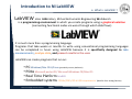
LabVIEW alias LABoratory Virtual Instruments Engineering Workbench
is a programming environment in which you create programs using a graphical notation (connecting functional nodes via wires through which data flows)
It is much more than a programming language
Programs that take weeks or months to write using conventional programming languages
can be completed in hours using LabVIEW because it is specifically designed to take
measurements, analyze data, and present results to the user.
LabVIEW can create programs that run on:
• PC Windows/Mac OS X/Linux (portability across platforms)
• PDAs Microsoft pocket PC/ Microsoft Windows CE/Palm OS • Real Time Platform NI cRIO
• Embedded systems FPGAs/DSPs/32‐bit Microprocessor (Blackfin from Analog Devices)
Università degli Studi di Catania
DIEEI
Introduction to NI LabVIEW
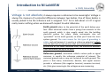
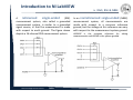
What is LabVIEW ? – Real vs Virtual Instruments
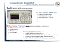
Real Instrument (Agilent digital scope)
“Pre‐defined” User Interface
• Buttons (boolean input)
• Knobs (numeric input)
• Display (graphical output)
• …
• …
Behaviour & Features strictly related on hardware architecture
•
•
•
•
•
ADC (resolution/sampling rate)
Microprocessor
Memory
A mid‐range Digital Scope can (at least):
Input/Output • Display Waveform (tipically up to 4)
…
• Perform basic measurement (time/amplitude/frequency domain)
• Connect to external equipment (GPIB/Ethernet/USB)
• Store data on external memory (usually in binary or ASCII)
Università degli Studi di Catania
DIEEI
Introduction to NI LabVIEW
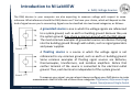
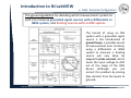
What is LabVIEW ? – Real vs Virtual Instruments
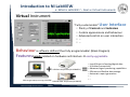
Virtual Instrument
“Fully customizable” User Interface
• Plenty of Controls and Indicators
• Custom appeareance and behaviour
• Advanced control on user interaction
• …
• …
Behaviour is software defined thus fully programmable! (Block Diagram)
Features loosely related on hardware architecture easily upgradable
+
Mid‐range Laptop running LabVIEW
Università degli Studi di Catania
USB Data Acquisition (NI‐USB 6251)
PCMCIA Data Acquisition (NI‐6062E)
DIEEI
=
• Input/Output of analog/digital data • Unlimited connectivity
• Advanced signal processing capabilities
• Efficient and flexible data storage
• Automatic report generation
•…
•…
Main features and advantages
Università degli Studi di Catania
DIEEI
Introduction to NI LabVIEW
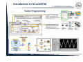
Faster Programming
Università degli Studi di Catania
DIEEI
LabVIEW main features 1/6
Introduction to NI LabVIEW
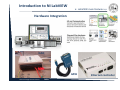
LabVIEW main features 2/6
Hardware Integration
DAQ
GPIB
Università degli Studi di Catania
DIEEI
Ethernet controller
Introduction to NI LabVIEW
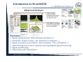
LabVIEW main features 3/6
Advanced Analysis
Examples:
Spectral analysis (FFT, PSD, harmonic distortion…)
Stochastic analysis (mean, std, covariance, histogram…)
Signal operations (convolution, deconvolution, cross‐correlation…)
Data filtering and numeric signal processing (Digital Signal Processing)
Signal conditioning
Data fitting and interpolation
Università degli Studi di Catania
DIEEI
Introduction to NI LabVIEW
LabVIEW main features 4/6
Multiple Targets & OSs
Portable devices
Microcontrollers
Multicore interface
Università degli Studi di Catania
DIEEI
FPGA
Introduction to NI LabVIEW
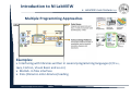
LabVIEW main features 5/6
Multiple Programming Approaches
Examples:
Interfacing with libraries written in several programming languages (C/C++, Java, Fortran, Visual Basic and so on)
Matlab .m files interface
DLLs (Dinamic‐Link Libraries) loading
Università degli Studi di Catania
DIEEI
Introduction to NI LabVIEW
User Interfaces
Università degli Studi di Catania
DIEEI
LabVIEW main features 6/6
Introduction to NI LabVIEW
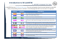
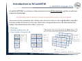
LabVIEW development system architecture
Embedded Design
Control Design & Simulation
Real‐Time module
Real‐Time Execution Trace Toolkit
FPGA module
Microprocessor SDK
Statechart module
Mobile module
DSP module
Embedded module for ADI Blackfin Processors
Embedded Module for ARM Microcontrollers Control Design and Simulation module
Fuzzy Logic Toolkit
Simulation Interface module
System Identification toolkit
Software Development & Deployment
Application Builder for Windows
VI Analyzer toolkit
Desktop Execution Trace toolkit
Remote panels
Requirements Gateway
Unit Test Framework Toolkit
Report Generation & Data Storage
SignalExpress
Report Generation Toolkit for Microsoft Office
Database Connectivity Toolkit
DataFinder Toolkit
Internet Toolkit
Image & Signal Processing
Vision Development Mathscript RT module
Advanced Signal Processing toolkit
Sound & Vibration Measurement suite
Spectral Measurement suite
Modulation toolkit
Vision Builder for Automated Inspection
Math Interface Toolkit
Industrial Monitoring & Control
Datalogging and Supervisory Control module
Wireless Sensor Network module
Touch Panel module
Motion Assistant
Softmotion module
LabVIEW core development system
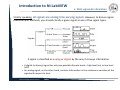
The NI LabVIEW product family consists of the LabVIEW development environment and more than 25 add‐on software tools that extend LabVIEW graphical programming for specific applications.
Università degli Studi di Catania
DIEEI
Environment
Università degli Studi di Catania
DIEEI
Introduction to NI LabVIEW
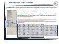
Introduction to Virtual Instruments: Front Panel
LabVIEW programs are called virtual instruments (VI) because their appearance and operation imitate physical instruments, such as
oscilloscopes and multimeters. Every VI uses functions that manipulate input from the user interface or other sources and display that
infromation or move to other file or other computers.
LabVIEW User Manual
A VI contains the following three components:
•
•
•
Front panel – Serves as the user interface
Block diagram – Contains the graphical source code (G language) that defines the functionality of the VI
Icon and connector panel – Identifies the VI so that you can use the VI in another VI. A VI within another VI is called subVI. A subVI corresponds to a subroutine in text‐based programming languages. You build the front panel with controls
and indicators, which are the interactive input and output terminals
of the VI, respectively. Controls are knobs, push buttons, dials, and other
input devices. Indicators are graphs, LEDs, and other displays. Controls
simulate instruments input devices
and supply data to the block diagram of
the VI. Indicators simulate instrument
output devices and display data the block diagram acquires or generates. Università degli Studi di Catania
DIEEI
Introduction to NI LabVIEW
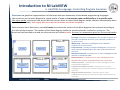
Introduction to Virtual Instruments: Block Diagram
LabVIEW programs are called virtual instruments (VI) because their appearance and operation imitate physical instruments, such as
oscilloscopes and multimeters. Every VI uses functions that manipulate input from the user interface or other sources and display that
information or move to other file or other computers.
LabVIEW User Manual
A VI contains the following three components:
•
•
•
Front panel – Serves as the user interface
Block diagram – Contains the graphical source code (G language) that defines the functionality of the VI
Icon and connector panel – Identifies the VI so that you can use the VI in another VI. A VI within another VI is called subVI. A subVI corresponds to a subroutine in text‐based programming languages. After you build the front panel, you add
code using graphical representations of
functions to control the front panel
objects. The block diagram contains this
graphical source code
Università degli Studi di Catania
DIEEI
Introduction to NI LabVIEW
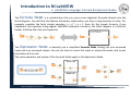
Introduction to Virtual Instruments: Icon & Connection Panel
LabVIEW programs are called virtual instruments (VI) because their appearance and operation imitate physical instruments, such as
oscilloscopes and multimeters. Every VI uses functions that manipulate input from the user interface or other sources and display that
infromation or move to other file or other computers.
LabVIEW User Manual
A VI contains the following three components:
•
•
•
Front panel – Serves as the user interface
Block diagram – Contains the graphical source code (G language) that defines the functionality of the VI
Icon and connection pane – Identifies the VI so that you can use the I in another VI. A VI within another VI is
called subVI. A subVI corresponds to a subroutine in text‐based programming languages. Icon
The Icon identifies the VI so you can use
it in another VI
The connector pane is a set of terminals
that corresponds to the controls and indicators of that VI, similar to the parameter list of a function call in text‐
based programming languages. The connector pane defines the inputs and outputs you can wire to the VI
Connection pane
Università degli Studi di Catania
DIEEI
G‐Language principal components
Università degli Studi di Catania
DIEEI
Introduction to NI LabVIEW
LabVIEW G‐Language: Function & Interface
double myFunction (double* a, int size)
{
double result = 0;
Black‐box approach; we only need the prototype
int tempSize = size;
double*
while (tempSize-->0)
myFunction
double
result += *a++;
int
return result/size;
INPUTS
}
1D array of double
OUTPUTS
double scalar
int scalar
The connection pane of LabVIEW nodes plays the same role of the function prototype in a traditional text‐based programming language
Università degli Studi di Catania
DIEEI
Introduction to NI LabVIEW
LabVIEW G‐Language: Data Types
In LabVIEW there are 32 different data types. The color and symbol of each terminal indicate the data type of the corresponding control or indicator. In the following table the 9 most common are reported. Control
Indicator
Description
Float. Double‐precision, floating‐point numeric
Integer. 32‐bit signed integer numeric
Boolean. Stores Boolean (TRUE/FALSE) values.
String. Provides a platform‐independent format for information and data, which you can use to create simple text messages, pass and store numeric data, and so on.
Array. Encloses the data type of its elements in square brackets and takes the color of that data type. As you add dimensions to the array, the brackets become thicker.
Cluster. Encloses several data types. Cluster data types appear brown if all elements in the cluster are numeric or pink if all elements of the cluster are of different types. Error code clusters appear dark yellow, while LabVIEW class clusters are crimson by default or teal green for Report Generation VIs.
Dynamic data. (Express VIs) Includes data associated with a signal and the attributes that provide information about the signal, such as the name of the signal or the date and time the data was acquired.
Waveform. Carries the data, start time, and t of a waveform.
I/O. Passes resources you configure to I/O VIs to communicate with an instrument or a measurement device.
Università degli Studi di Catania
DIEEI
Introduction to NI LabVIEW
LabVIEW G‐Language: Nodes
Nodes are objects on the block diagram that have inputs and/or outputs and perform
operations when a VI runs.
They are analogous to statements, operators, functions, and subroutines in text‐
based programming languages. LabVIEW includes the following types of nodes:
• Functions—Built‐in execution elements, comparable to an operator,
function, or statement.
• SubVIs—VIs used on the block diagram of another VI, comparable to
subroutines.
• Express VIs—SubVIs designed to aid in common measurement tasks. You
configure an Express VI using a configuration dialog box.
• Structures—Execution control elements, such as For Loops, While Loops,
Case structures, Flat and Stacked Sequence structures, Timed structures, and
Event structures.
• Formula and Expression Nodes—Formula Nodes are resizable structures for
entering equations directly into a block diagram. Expression Nodes are
structures for calculating expressions that contain a single variable.
Università degli Studi di Catania
DIEEI
Introduction to NI LabVIEW
LabVIEW G‐Language: Express VIs
An Express VI is a VI whose settings you can configure interactively through a dialog box. Express VIs appear on the block diagram as expandable nodes with icons surrounded by a blue field.
You can configure an Express VI by setting options in the configuration dialog box that appears when you place the Express VI on the block diagram.
The primary benefit of Express VIs is their interactive configurability. Express VIs are useful when you want to give users a VI or library of VIs for building their own applications easily with minimal programming expertise.
Express VIs do not provide run‐time interactive configuration for VIs. If you need run‐time reconfiguration, build an application with a user interface that contains features similar to a configuration dialog box. Express VIs are designed for ease of use. If you need an application to run with strict memory restrictions or high execution speeds, use standard VIs.
Università degli Studi di Catania
DIEEI
Introduction to NI LabVIEW
LabVIEW G‐Language: Controlling Program Execution
Structures are graphical representations of the loops and case statements of text‐based programming languages. Use structures on the block diagram to repeat blocks of code and to execute code conditionally or in a specific order. Like other nodes, structures have terminals that connect them to other block diagram nodes, execute automatically when input data is available, and supply data to output wires when execution completes. Each structure has a distinctive, resizable border to enclose the section of the block diagram that executes according to the rules of the structure. The section of the block diagram inside the structure border is called a subdiagram. The terminals that feed data into and out of structures are called tunnels. A tunnel is a connection point on a structure border.
For loop
While loop
Flat sequence
structure
Stacked sequence
structure
Università degli Studi di Catania
DIEEI
Case structure
Event
Structure
For Loop—Executes a subdiagram a set number of times or, if you add a conditional terminal, until a Boolean condition or an error occurs. While Loop—Executes a subdiagram until a Boolean condition or an error occurs. Case structure—Contains multiple subdiagrams, only one of which executes depending on the input value passed to the structure. Sequence structure—Contains one or more subdiagrams that execute in sequential order. Event structure—Contains one or more subdiagrams that execute when events are generated by user interaction. Timed structures—Execute one or more subdiagrams with time bounds and delays. Conditional Disable structure—Contains one or more subdiagrams, exactly one of which compiles and executes at run‐time. Diagram Disable structure—Contains one or more subdiagrams, exactly one of which compiles and executes at run‐time. Introduction to NI LabVIEW
LabVIEW G‐Language: Formula & Expression Nodes
The Formula Node is a resizable box that you use to enter algebraic formulas directly into the
block diagram. You will find this feature extremely useful when you have a long formula to solve. For
example, consider the fairly simple equation, y = x2 + x + 1. Even for this simple formula, if you
implement this equation using regular LabVIEW arithmetic functions, the block diagram is a little bit
harder to follow than the text equations
The Expression Node is basically just a simplified Formula Node having just one unnamed
input and one unnamed output. You do not have to name the input or output terminals and to put
semicolons at the end.
The same operators and syntax of the Formula Node apply to the Expression Node.
Università degli Studi di Catania
Introduction to NI LabVIEW
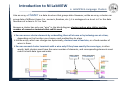
LabVIEW G‐Language: Array
array
A LabVIEW is a collection of data elements that are all the same type, just like in traditional programming languages.
An array data element can have any type except another array, a chart, or a graph.
Array elements are accessed by their indices; each element's index is in the range 0 to N‐1, where N is the total number of elements in the array. Notice that, along each dimension, the first element has index 0, the second element has index 1, and so on.
Data type
Number of dimensions, D
Total number of elements, N
1.23
0.67
3x1
D = 1
N = 3
‐34
I: {i}
i=0:1
Università degli Studi di Catania
We access the array elements by DxN indices, I
1.23
1.90
0.67
12
‐34
0.25
3x2
D = 2
N = 6
I: {i,j}
i=0:2, j=0:1
DIEEI
2x3x3
D = 3
N = 18
I: {i,j,k}
i=0:1, j=0:2, k=0:2
Introduction to NI LabVIEW
LabVIEW G‐Language: Clusters
Like an array, a cluster is a data structure that groups data. However, unlike an array, a cluster can group data of different types (i.e., numeric, Boolean, etc.); it is analogous to a struct in C or the data members of a class in C++ or Java. Because a cluster has only one "wire" in the block diagram clusters reduce wire clutter and the number of connector terminals that subVIs need
You can access cluster elements by unbundling them all at once or by indexing one at a time, depending on the function you choose; each method has its place Unlike arrays, which can change size dynamically, clusters have a fixed size, or a fixed number of wires in them.
You can connect cluster terminals with a wire only if they have exactly the same type; in other words, both clusters must have the same number of elements, and corresponding elements must match in both data type and order.
Bundle
Università degli Studi di Catania
DIEEI
Unbundle
Labview in a measurement scenario
Università degli Studi di Catania
DIEEI
Introduction to NI LabVIEW
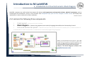
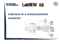
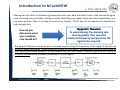
The typical measurement scenario
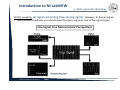
• Sensors and transducers detect physical phenomena. • Signal conditioning components condition physical phenomena so that the measurement device can receive data. • The computer receives the data through the measurement device. • Software controls the measurement system, telling the measurement device when and from which channels to acquire or generate data. • Software also takes the raw data, analyzes it, and presents it in a form you can understand, such as a graph, chart, or file for a report.
MAX+NI‐DAQmx
Università degli Studi di Catania
DIEEI
DAQ: overview
Introduction to NI LabVIEW
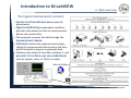
DAQ: signals & information
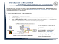
Strictly speaking, all signals are analog time‐varying signals. However, to discuss signal
measurement methods, you should classify a given signal as one of five signal types.
A signal is classified as analog or digital by the way it conveys information. • A digital (or binary) signal has only two possible discrete levels—high level (on) or low level (off). • An analog signal, on the other hand, contains information in the continuous variation of the signal with respect to time. Università degli Studi di Catania
DIEEI
Introduction to NI LabVIEW
DAQ: signals & information
Strictly speaking, all signals are analog time‐varying signals. However, to discuss signal measurement methods, you should classify a given signal as one of five signal types. One Signal, Five Measurement Perspectives
Università degli Studi di Catania
DIEEI
Introduction to NI LabVIEW
DAQ: Hardware
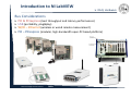
Bus Considerations
PCI & PCIexpress (best throughput and latency performances)
USB (portability, plug&play)
WI/FI – Ethernet (wireless or wired remote measurement)
PXI – PXIexpress (modular, high‐bandwidth open‐PC based platform) Università degli Studi di Catania
DIEEI
Introduction to NI LabVIEW
16‐ or 18‐bit, up to 1.25 MS/s, up to 80 analog inputs
Up to 4 analog outputs at 16 bits, 2.8 MS/s (2 µs full‐scale settling)
Up to 48 TTL/CMOS digital I/O lines (up to 32 hardware‐timed at 10 MHz)
Two 32‐bit, 80 MHz counter/timers
NI‐DAQmx driver software and NI LabVIEW SignalExpress LE interactive data‐logging software
NI‐MCal calibration technology for improved measurement accuracy by up to 5X
Università degli Studi di Catania
DIEEI
DAQ: M‐Series
Introduction to NI LabVIEW
LabVIEW G‐Language: DAQ concepts
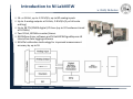
Virtual channels define real‐world measurements consisting of one
or more DAQ channels (terminals on your DAQ device) along with
other channel‐specific information: range, terminal configuration,
and custom scaling that is used to format the data.
An NI‐DAQmx Task is a collection of one or more virtual channels
along with timing, triggering, and other properties. Conceptually, a
task represents a measurement or generation you want to perform.
For example, a task allows you to specify whether you want to
measure 1 sample, measure N samples, or measure continuously
(using a buffer to store data). A task also allows you to specify the
sample rate, the timing clock source, and the task triggers. Once
you have defined a task, you can simply start the task, read the task
data, and stop the task from within LabVIEW.
Università degli Studi di Catania
DIEEI
Introduction to NI LabVIEW
DAQ: Grounding
Voltage is not absolute; it always requires a reference to be meaningful. Voltage is
always the measure of a potential difference between two bodies. One of these bodies is
usually picked to be the reference and is assigned "0 V." So to talk about a 3.47 V signal
really means nothing unless we know with respect to what reference.
Earth ground refers to the potential of the earth below your
feet. Most electrical outlets have a prong that connects to the
earth ground, which is also usually wired into the building
electrical system for safety. Many instruments also are
"grounded" to this earth ground, so often you'll hear the term
system ground. The main reason for this type of grounding is
safety, and not because it is used as a reference potential. In fact,
you can bet that no two sources that are connected to the earth
ground are at the same reference level; the difference between
them could easily be up to 10 volts.
Reference ground, sometimes called a return path or signal
common, is usually the reference potential of interest. The
common ground may or may not be wired to earth ground. The
point is that many instruments, devices, and signal sources
provide a reference (the negative terminal, common terminal,
etc.) that gives meaning to the voltages we are measuring.
Università degli Studi di Catania
DIEEI
Introduction to NI LabVIEW
DAQ: Voltage Sources
The DAQ devices in your computer are also expecting to measure voltage with respect to some
reference. What reference should the DAQ device use? You have your choice, which will depend on the
kind of signal source you're connecting. Signals can be classified into two broad categories, as follows:
A grounded source is one in which the voltage signals are referenced to a system ground, such as earth or building ground. Because they use the system ground, they share a common ground with the DAQ device. The most common examples of grounded sources are devices that plug into the building ground through wall outlets, such as signal generators and power supplies.
A floating source is a source in which the voltage signal is not
referenced to any common ground, such as earth or building ground.
Some common examples of floating signal sources are batteries,
thermocouples, transformers, and isolation amplifiers. Notice that
neither terminal of the source is connected to the electrical outlet
ground. Thus, each terminal is independent of the system ground.
To measure your signal, you can almost always configure your DAQ device to make measurements that fall into one of these three categories: Differential, Referenced Single Ended, Nonreferenced Single‐Ended
Università degli Studi di Catania
DIEEI
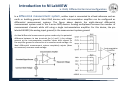
Introduction to NI LabVIEW
DAQ: Differential terminal configuration
In a differential measurement system, neither input is connected to a fixed reference such as
earth or building ground. Most DAQ devices with instrumentation amplifier can be configured as
differential measurement systems. The figure above depicts the eight‐channel differential
measurement system used in the E‐series DAQ devices. Analog multiplexers increase the number of
measurement channels while still using a single instrumentation amplifier. For this device, the pin
labeled AIGND (the analog input ground) is the measurement system ground.
An ideal differential measurement system reads only the potential
difference between its two terminals the (+) and (‐). Any voltage
present at the instrumentation amplifier inputs with respect to
the amplifier ground is referred to as a common‐mode voltage. An
ideal differential measurement system completely rejects (does
not measure) common‐mode voltage.
Università degli Studi di Catania
DIEEI
Introduction to NI LabVIEW
A
referenced single‐ended (RSE)
measurement system, also called a grounded
measurement system, is similar to a grounded
signal source, in that the measurement is made
with respect to earth ground. The figure above
depicts a 16‐channel RSE measurement system.
Università degli Studi di Catania
DIEEI
DAQ: RSE & NRSE
In an nonreferenced single‐ended (NRSE)
measurement system, all measurements are
made with respect to a common reference
ground, but the voltage at this reference can vary
with respect to the measurement system ground.
AISENSE is the common reference for taking
measurements and AIGND is the system ground.
Introduction to NI LabVIEW
DAQ: Terminal Configuration
The general guideline for deciding which measurement system to pick is to measure grounded signal sources with a differential or NRSE system, and floating sources with an RSE system.
The hazard of using an RSE
system with a grounded signal
source is the introduction of
ground loops, a possible source
of measurement error. Similarly,
using a differential or NRSE
system to measure a floating
source will very likely be
plagued by bias currents, which
cause the input voltage to drift
out of the range of the DAQ
device (although you can
correct this problem by placing
bias resistors from the inputs to
ground).
Università degli Studi di Catania
DIEEI
Introduction to NI LabVIEW
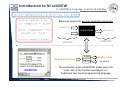
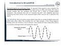
DAQ: Sampling
Real‐world signals are continuous things. To represent these signals in your computer, the
DAQ device has to check the level of the signal every so often and assign that level a
discrete number that the computer will accept; this is called an analog‐to‐digital
conversion. The computer then sort of "connects the dots" and, hopefully, gives you
something that looks similar to the real‐world signal (that's why we say it represents the
signal).
The sampling rate of a system simply reflects how often an analog‐to‐digital conversion
(ADC) takes place. When the sampling rate isn't high enough, a scary thing happens.
Aliasing, while not intuitive, is easy to observe. If we sample 8.5 times slower (the circles),
our reconstructed signal looks nothing like the original.
Università degli Studi di Catania
DIEEI
Introduction to NI LabVIEW
DAQ: ADC & DAC
Aliasing has the effect of introducing frequencies into your data that didn't exist in the real‐world signal
(and removing some that did), thereby severely distorting your signal. Once you have aliased data, you
can never go back: There is no way to remove the "aliases." That's why it's so important to sample at a
high‐enough rate.
Nyquist's Theorem
How do you determine what your sampling rate should be? To avoid aliasing, the sampling rate must be greater than twice the maximum frequency component in the signal to be acquired.
The Nyquist Theorem only deals with accurately representing the frequency of the signal. It doesn't say
anything about accurately representing the shape of your signal. To adequately preserve the shape of
your signal, you should sample at a much higher rate than the Nyquist frequency, generally at least 5 or
10 times the maximum frequency component of your signal.
Università degli Studi di Catania
DIEEI
Introduction to NI LabVIEW
DAQ: NI HW comparison Example
Input analogico
Numero di canali
Frequenza di campionamento
Risoluzione
Campionamento simultaneo
Intervallo massimo di tensione
Intervallo di accuratezza
Intervallo minimo di tensione
Intervallo di accuratezza
Output analogico
Numero di canali
Velocità di aggiornamento
Risoluzione
Intervallo massimo di tensione
Intervallo di accuratezza
Intervallo minimo di tensione
Intervallo di accuratezza
I/O digitale
Numero di canali
Temporizzazione
Livelli di logica
Intervallo input massimo
Intervallo output massimo
Contatori/Timer
Numero di Contatori/Timer
Risoluzione
Frequenza di origine massima
Minima ampiezza di impulsi input
Livelli di logica
Intervallo massimo
Università degli Studi di Catania
DIEEI
8 SE/4DI
48 kS/s
14 bits
No
‐10..10 V
138 mV
‐1..1 V
37.5 mV
16 SE/8 DI
1.25 MS/s 16 bits
No
‐10..10 V 1920 µV ‐100..100 mV
52 µV 2
150 S/s
12 bits
0..5 V
7 mV
0..5 V
7 mV
2
2.86 MS/s 16 bits
‐10..10 V 2080 µV ‐5..5 V 1045 µV 12 DIO
Software
TTL
0..5 V
0..5 V
24 DIO Hardware, Software TTL
0..5 V
0..5 V
1
32 bits
5 MHz
100 ns
TTL
0..5 V
2
32 bits
80 MHz
12.5 ns
TTL
0..5 V