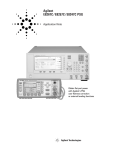
1
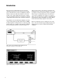
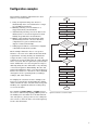
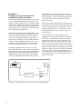
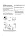
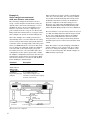
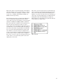
Obtaining Flat
Test Port Power
with the Agilent
8360’s User Flatness
Correction Feature
Product Note 8360-2
Introduction
The 8360 series synthesized sweepers provide
extremely flat power at your test port, for testing
power sensitive devices such as amplifiers, mixers,
diodes or detectors. The user flatness correction
feature of the 8360 synthesized sweepers compensates for attenuation and power variations created by
components between the source and the test device.
User flatness correction allows the digital correction
of up to 801 frequency points (1601 points via GPIB),
in any frequency or sweep mode (i.e., start/stop, CW,
power sweep, etc.). Using a power meter to calibrate
the measurement system, as shown in figure 1, a
Figure 1. Basic system configuration using an 437B power meter
for automatic user flatness correction data entry
Figure 2. 8360 displaying the user flatness correction table
2
table of power level corrections is created for the
frequencies where power level variations or loss occur
(see figure 2). These frequencies may be sequential
linear steps or arbitrarily spaced. To allow the
correction of multiple test setups or frequency
ranges, the user may save as many as eight different
measurement setups (including correction tables)
in the internal storage registers of the 8360.
This note illustrates how to utilize the user flatness correction feature by providing step-by-step
instructions for several common measurement
examples.
Theory of operation
A major contribution of the 8360 series synthesized
sweepers is their unparalleled leveled output
power accuracy and flatness. This is achieved by
using a digital (vs. analog) design to control the
internal automatic leveling circuitry (ALC).
An internal detector samples the output power
to provide a DC feedback voltage. This voltage is
compared to a reference voltage that is proportional
to the power level chosen by the user. When there
is a discrepancy between voltages, the power is
increased or decreased until the desired output level
is achieved (see figure 3). The factory-generated
internal calibration data of an 8360 is digitally
segmented into 1601 data points across the start/stop
frequency span set by the user. Subsequently, these
points are converted into 1601 reference voltages
for the ALC loop.
Oscillator
Pin
modulator
Power
amplifier
The digital ALC control scheme not only delivers
excellent power accuracy and flatness at the output
port of the instrument, but also provides the means
to execute the user flatness correction feature of the
8360. Generally, a power meter is used to create a
table of correction data that will produce flat power
at the test port. The user may measure and enter
correction data for up to 801 points. The correction
data contained in the table is linearly interpolated
to produce a 1601-point data array across the
start/stop frequency span set on the source. This
is summed with the internal calibration data of the
8360 (see figure 4). When user flatness correction
is enabled, the sum of the two arrays will produce
the 1601 reference voltages for the ALC loop.
Step
attenuator
Leveled
RF output
To
test
port
Correction
voltage
Detector
Leveling
amplifier
Feedback
voltage
Referece
voltage
Figure 3. Simplified automatic leveling circuitry
1601 equadistant
point array
accessable only
from a computer
User flatness correction array
1 to 801 point frequencycorrection pairs entered
from a computer
or the front panel
1601 points of internal
calibration data
Complete
1601 point
array
On
CorPair
disable
Fitness
on/off
Off
Linear
interpolation
1601 points
of correction
data
1601 points
of calibration
data
∑
1601
points
for ALC
DAC
Figure 4. ALC calibration correction - summing user flatness correction array
with internal calibration array
3
If the correction frequency span is only a subset of
the start/stop frequency span set on the source, no
corrections will be applied to the portion of the
sweep that is outside the correction frequency span.
The following example illustrates how the data is
distributed within the user flatness correction array.
When utilizing user flatness correction, do not exceed
the 8360 ALC operating range. Exceeding the ALC
range will cause the output power to become
unleveled and eliminate the benefits of user flatness
correction. The ALC range can be determined by
subtracting the minimum output power (-20 dBm)
from the maximum specified power1. An Agilent
83620B has an ALC range of ≥30 dB (≥+10 to
-20 dBm).
Assume that the user sets up the source to
sweep from 2 to 18 GHz but only enters user
flatness correction data from 14 to 18 GHz.
Linear interpolation will occur between the
correction entries to provide the 401 points
required for the 14 to 18 GHz portion of the
array. No corrections will be applied to the
2 to 13.99 GHz portion of the array.
Point number
1200
0
No corrections applied
2 GHZ
1600
401 pts. data
14 GHz 18 GHz
1st corr. freq.
Frequency
Number of points interpolated between
correction entries:
freq span between correction entries
x 1600 – 1 = # pts
stop frequency – start frequency
When correction frequencies are arbitrarily
spaced, the number of interpolated points
will vary.
When user flatness correction is enabled, the
maximum settable test port power is equivalent to
the maximum available leveled power minus the
maximum path loss (P0 max -Ppath loss). For
example, if an 83620B has a maximum path loss
of 15 dB due to system components between the
source output and the test port, the test port power
should be set to -5 dBm. When user flatness correction is enabled, this will provide the maximum
available power to the device under test (DUT).
The following glossary reviews the terms that will
be used throughout this note:
array - the 1601 user flatness correction points that
will be summed with the internal calibration data
of the Agilent 8360. The array covers the entire
start/stop frequency range the user sets on the
instrument.
correction table – the user-supplied entries in
the array. Each entry in the table has a correction
component and an associated frequency component.
user flatness correction
correction frequency – the frequency component of
an entry where a correction has been or will be
measured and entered in the table.
correction frequency span – the frequency span
between the first and last correction frequency.
correction data – the power level correction
components of entries in the table.
cal factor – the calibration factors displayed on the
power sensor. By entering the appropriate cal factor for each measurement frequency on a power
meter, one can calibrate the power meter to a particular power sensor across the chosen frequency
range.
Figure 5. Array configuration example
1
4
When the optional step attenuator is ordered on an 8360 with firmware released prior to November 1990, the attenuator will need to be uncoupled if the full
ALC range is required. This can be accomplished by selecting POWER [MENU] [Uncoupl Atten].
Configuration examples
The following examples demonstrate the user
flatness correction feature:
1. Using an Agilent 437B power meter to
automatically enter correction data for a swept
2 to 18 GHz measurement.
2. Manually entering correction data for a
stepped (list mode) measurement.
3. Automatically entering correction data for an
arbitrary list of correction frequencies when
making swept mm-wave measurements.
4. Making scalar analysis measurements with
automatically-entered correction data that
compensates for power variations at the
output of a directional bridge.
5. Setting up user flatness corrections in computer
controlled measurement systems.
Each example illustrates how to set up user
flatness correction for a different measurement
requirement. You may modify the instrument
setups shown to suit your particular needs.
Completed correction tables may be easily edited if
more correction data is required for your measurement. Additional correction frequencies may be
added by using the auto fill feature or by entering
correction frequencies individually. The auto fill
feature will add but not delete correction frequencies.
Refer to the 8360 User’s Guide for a more detailed
description of the operating modes, hardkeys,
softkeys, and other features.
To simplify the execution of these examples, the
keys to be selected have been bracketed to differentiate them from other text. The 8360 front panel
hardkeys are capitalized, while the softkeys they
access are in italics.
For example: POWER [MENU] - POWER refers to
the source’s functional grouping, [MENU] refers to
the hardkey the user must select in that function.
Auto Fill [Start] - [Start] refers to the softkey the
user selects to enter the first correction frequency
for the auto fill feature.
Start
Setup source
Setup correction frequencies
Setup power meter
Connect sensor to test port
Is power
sensor's cal factor
set for active correction
frequency?
No
Enter cal factor
on power meter
Yes
Measure Power
Enter correction in table
Yes
Next
frequency?
No
Turn on user flatness correction
Set test port power
Save correction table
Reconnect device to test port
Make measurement
Stop
Figure 6. User Flatness Correction flowchart
5
Data entry methods
for user flatness correction
User flatness correction data is obtained by
connecting a power meter sensor at the desired
test port and calibrating the measurement system.
To make an accurate power meter measurement,
the power meter must be calibrated to the power
sensor by attaching the sensor to the "POWER REF"
output and performing a calibration. (It is assumed
that the user is already familiar with calibrating
and zeroing the power meter in use.) The accuracy
of the power meter measurement is also dependent
on the accuracy of the calibration factors used during
the measurement; the calibration factors must be
set for each individual correction frequency prior
to making the measurement. There are three methods
of user flatness correction data entry which are
primarily determined by the type of power meter
available.
A 437B power meter facilitates automatic entry of
correction data. Since the 8360 communicates with
the power meter over GPIB, it must be the system
controller during the data entry process. Only the
437B is capable of receiving frequency information
from the source, and incorporating the appropriate
power sensor calibration factor in the power measurement (the user should be familiar with selecting
and editing the calibration factor tables). The 8360
then retrieves the power measurement data and
inputs the appropriate correction data in the array.
For power meters other than the 437B, the test port
power must be manually measured at each correction
frequency. At any given correction frequency, the
user must enter the appropriate power sensor cal
factor, measure the power, and then enter the correction data in the user flatness correction array
from the front panel of the 8360 (see Example 2).
Automatic test systems may be programmed to
interrogate the source for the test frequency, enter
the appropriate power sensor cal factor, make the
power meter measurement (with any power meter),
and send the data to the source so it can place the
appropriate correction data in the table. The 437B is
recommended since it is capable of internally storing
the cal factor information for different power sensors.
Other power meters will require a look-up table of
power sensor cal factors in the program.
Figure 7. Basic system configuration using an 437B Power Meter for automatic User
Flatness Correction data entry
6
Example 1:
Swept measurement with
automatically entered corrections
This example illustrates how to set up a 2 to 18
GHz swept measurement with a correction frequency
every 100 MHz (see figure 1 for system configuration).
The auto fill feature is used to increment the correction frequencies across the entire measurement
range. A 437B power meter automatically enters
correction data into the array.
When additional correction points are desired, use the
auto fill feature to enter new correction frequencies
in the required portion of the frequency span. When
the 437B is used, the meter measurement menu’s
([Mtr Meas Menu]) Meas Corr [Undef] softkey may
be utilized to measure just the correction data for
the additional points. The correction table should
be cleared before entering an entirely new list of
correction frequencies.
This example assumes that there is a 5 dB path
loss in the measurement system attached to an
83620A. To provide the maximum available power
to the device under test, a test port power of +5
dBm is selected. With user flatness correction
enabled, the source will provide +10 dBm at the
RF output port and +5 dBm at the test port.
Command
Setup source parameters
[PRESET]
FREQUENCY [START] 2 GHz
FREQUENCY [STOP] 18 GHz
POWER [POWER LEVEL] 10 dBm
Description
Reset source to a known state
Set start frequency to 2 GHz
Set stop frequency to 18 GHz
Set power to +10 dBm
(maximum specified power)
Access user flatness correction menu
POWER [MENU]
Access power softkey menu
[more]
Display next softkey menu
[Fltness Menu]
Access flatness softkey menu
Clear flatness array
[Delete Menu]
Delete [All]
MENU SELECT [PRIOR]
[more]
Access delete array softkey menu
Clear array
Exit delete menu
Display previous softkey menu
Display next softkey menu
Enter frequencies in flatness array
Auto Fill [Start] 2 GHz
Set first frequency in user flatness
array to 2 GHz
Auto Fill [Stop] 18 GHz
Set last frequency of the user
flatness array to 18 GHz
Auto Fill [Incr] 100 MHz
Set frequency increment to every
100 MHz from 2 to18 GHz
Calibrate the power meter to the power sensor in use
Connect 437B’s power sensor to test port
Verify GPIB cable connection between source and power meter
Enter and store in the power meter the power sensor's cal factors for
correction frequencies in the array
[more]
Enter correction data into array
[Mtr Meas Menu]
Meas Corr [All]
Display next softkey menu
Access the automatic data entry
power meter menu
Input the correction data
Remove power meter sensor from test port; do not reconnect device
POWER [FLTNESS ON/OFF]
Enable user flatness correction
POWER [POWER LEVEL] 5 dBm
Set test port power +5 dBrn
(P0 max - Ppath loss)
[SAVE] n
Save the source parameters including
the correction table in an internal
register
Reconnect device under test
7
Example 2:
Frequency list measurement with
manually entered corrections
the appropriate correction and enter it into the
table. If the user already has a table of correction
data prepared, it can be entered directly into the
correction table from the keypad on the front
panel of the 8360.
The following example demonstrates how to enter
correction data when using a power meter other
than the 437B (see figure 8 for the system configuration). This example also introduces two features
of the 8360: frequency follow, which simplifies the
data entry process, and list mode, which sets up a
list of arbitrary test frequencies.
With the list mode feature, the user may enter the
test frequencies into a table in any order and specify
an offset (power) and/or a dwell time for each
frequency. When list mode is enabled, the 8360
will step through the list of frequencies in the
order entered.
The frequency follow feature automatically sets the
source to a CW test frequency equivalent to the
active correction frequency in the user flatness
correction table. The front panel arrow keys are
used to move around the correction table and enter
correction data. Simultaneously, the source test
frequency is updated to the selected correction
frequency without exiting the correction table.
The user flatness correction feature has the
capability of copying and entering the frequency
list into the correction table. Since the offset in
the list mode table is not active during the user
flatness correction data entry process, the value
of the correction data will be determined as if no
offset is entered. When user flatness correction and
list mode (with offsets) are enabled, the 8360 will
adjust the output power by an amount equivalent
to the sum of the correction data and offset for
each test frequency. The user must make sure that
the resulting power level is still within the ALC
range of the source.
To further simplify the data entry process, the
8360 allows the user to enter correction data into
the user flatness correction table by adjusting the
front panel knob until the desired power level is
displayed on the power meter. The user flatness
correction algorithm will automatically calculate
8360
synthesized sweeper
Power meter
Test port
Power sensor
Cables, switches,
etc.
DUT
Figure 8. Basic system configuration for applications using a power meter other than the 437B
8
Command
Description
Setup source parameters
[PRESET]
Reset source to a known state
POWER [POWER LEVEL] 5 dBm Set test port power to +5 dBm (P0 max - Ppath loss)
Create frequency list
FREQUENCY[MENU]
[more]
[Fltness Menu]
Enter List [Freq] 5 GHz
Access the frequency softkey menu
Display next softkey menu
Access the frequency list softkey menu
Enter 5 GHz as the first frequency
Entering a frequency automatically sets the offset and dwell to 0 dB and 10 ms, respectively
Enter 18, 13, 11, and 20 GHz from the keypad
Access user flatness correction menu
POWER [MENU]
Access power softkey menu
[more]
Display next softkey menu
[Fltness Menu]
Access flatness softkey menu
Clear flatness array
[Delete Menu]
Delete [All]
MENU SELECT [PRIOR]
[more]
[more]
[Copy List]
[Freq Follow]
[more]
Access delete array softkey menu
Clear array
Leave delete menu
Display previous softkey menu
Display next softkey menu
Display next softkey menu
Copy the frequency list into the correction table in a sequential order
Set source to the active correction frequency in the flatness array
(i.e when the arrow points to the 5 GHz correction data point in the
correction table, the source is also set to a CW frequency of 5 GHz)
Display next softkey menu
Calibrate the power meter to the power sensor in use
Connect power meter sensor to test port
Enter the cal factor for first correction frequency (5 GHz)
➮
Enter correction data into table
POWER [FLTNESS ON/OFF]
Enable User Flatness Correction; power meter will display
corrected data
Enter [Corr]
Enter correction data - rotate knob until power meter displays
desired power level (5 dBm)
Allow entry of next frequency correction
Enter in the power meter the sensor's cal factor for the next frequency in the array
Repeat until each correction has been entered
[SAVE]n
Save the source parameters including the correction table in an
internal register
Remove power meter sensor from test port and reconnect device
Activate List Mode
SWEEP [MENU]
Sweep Mode [List]
Access sweep softkey menu
Select frequency list mode
9
Example 3:
Swept mm-wave measurement with
arbitrary correction frequencies
between non-sequential correction frequencies will
vary. This example uses the 437B to automatically
enter correction data into the array.
The focus of this example is on using user flatness
correction to obtain flat power at the output of the
Agilent 83550 series mm-wave source modules. In
this case we will use non-sequential correction
frequencies in a swept 26.5 to 40 GHz measurement
with an 83554 source module.
Note: Turn off the 8360 prior to connecting the
source module interface (SMI) cable, or damage
may result.
Configure the measurement system as shown in
figure 9a or 9b. When the 8360 is preset, the
following occurs:
It is time consuming to perform large quantities of
power meter measurements. To reduce this time, we
will select non-sequential correction frequencies in
order to target specific points or sections of the
measurement range that we will assume are more
sensitive to power variations. This will greatly
expedite setting up the user flatness correction
table. The amount of interpolated correction points
• The source module’s frequency span is
displayed on the source.
• The 8360 leveling mode is automatically
changed from internal to "module leveling."
• The source module's maximum specified
power is set and displayed.
437B
power meter
83623B/83624B
synthesized sweepers
GPIB
Test port
R8486A
power sensor
RF out
Source module
interface
RF in
83554A
source module
(a)
DUT
83620B/83622B/
83640B/83642B
synthesized sweepers
437B
power meter
GPIB
RF out
8349B
microwave
amplifier
RF
out
Test port
RF in
Source module
interface
R8486A
power sensor
RF in
(b)
83554A
source module
DUT
Figure 9. (a) mm-wave module hookup diagram with high power 8360 (83623B/24B),
(b) hookup diagram with standard 8360 using an Agilent 8349B amplifier
10
Command
Description
Turn off source
Connect Source Module Interface cable
Turn on source
Setup source parameters
[PRESET]
FREQUENCY [START] 26.5 GHz
FREQUENCY [STOP] 40 GHz
POWER [POWER LEVEL] 7 dBm
Set start frequency to 26.5 GHz
Set stop frequency to 40 GHz
Set source module power to +7 dBm for maximum power to
device under test
Access User Flatness Correction Menu
POWER [MENU]
Access power softkey menu
[more]
Display next softkey menu
[Fltness Menu]
Access flatness softkey menu
Clear flatness array
[Delete Menu]
Delete [All]
MENU SELECT [PRIOR]
Access delete array softkey menu
Clear array
Exit delete menu
Display previous softkey menu
Enter non-sequential frequencies into array
Enter [Freq] 26.5 GH z
Enter 26.5 GHz as the first correction frequency in flatness array
Enter [Freq] 31 GHz
Enter 31 GHz as the second frequency
Enter [Freq] 32.5 GHz
Enter 32.5 GHz as the third frequency
Enter [Freq] 40 GHz
Enter 40 GHz as the last frequency
Calibrate the power meter to the power sensor in use
Connect 437B’s power sensor to test port
Verify GPIB cable connection between source and power meter2
Enter and store in the power meter, the power sensor's cal factors for correction frequencies in the array2
[more]
[more]
Enter correction data into array
[Mtr Meas Menu]
Meas Corr [All]
[SAVE] n
Display next softkey menu
Display next softkey menu
Access the automatic data entry power meter menu
Input the correction data
Save the source parameters including the correction table in an
internal register
Remove power meter sensor from test port and reconnect device
POWER [FLTNESS ON/OFF]
2
Enable user flatness correction
U, V and W band power sensors are not available from Agilent. For these frequency bands use the Anritsu ML83A Power Meter with the MP715-004 (40 to
60 GHz), the MP716A (50 to 75 GHz), or the MP81B (75 to 110 GHz) power sensors. Since the Anritsu ML83A is not capable of internally storing power
sensor cal factors, manual correction data entry is required (see Example 2).
11
Example 4:
Scalar analysis measurement
with user flatness corrections
When a 437B power meter is used to automatically
enter the correction data, the correction calibration routine will automatically turn off any active
modulation and then reactivate the modulation
upon the completion of the data entry process.
Therefore, the scalar pulse modulation that is automatically enabled in a scalar measurement system
will be disabled during a 437B correction calibration.
The following example demonstrates how to
setup a scalar analysis measurement (using an
Agilent 8757 scalar network analyzer) of a 2 to
20 GHz test device such as an amplifier. User
flatness correction is used to compensate for
power variations at the test port of a directional
bridge. Follow the instructions to set up the source,
then configure the system as shown in Figure 10.
Since this example uses a 437B power meter to
automatically enter correction data into the array,
it is necessary to turn off the 8757 system interface
so that the source can temporarily control the power
meter over GPIB. When the correction data entry
process has been completed, enable user flatness
correction and set the desired test port power
level. Then store the correction table and source
configuration in the same register that contains
the analyzer configuration. Reactivate the 8757 system interface and recall the stored register. Make
sure that user flatness correction is still enabled
before making the measurement.
Command
Description
[PRESET] source
Reset to a known state
Set the source to
Analyzer mode
SYSTEM [MENU]
[GPIB Menu]
Programming Language
[Analyzer]
83620B
synthesized sweeper
Sweep output
Z-axis blank/mkrs
Stop sweep in/out
8757C
scalar analyzer
85025E detector
11667B
power splitter
8485A
power sensor
Figure 10. Scalar system configuration
12
Sweep in
Pos Z blank
Stop sweep
8757 system interface
GPIB
Test port
437B
power meter
Note: The 8360’s rear panel language and address
switches must be set to 7 and 31 (all 1s), to allow
the user to change the language or address of the
source via the front panel. The default settings are
TMSL and 19, respectively.
Access system softkey menu
Access GPlB softkey menu
Select analyzer language as the
instrument's external interface language
Asterisk = active function
GPIB
RF output
The user flatness correction array cannot be stored
to a disk. You must make sure that the array is stored
in one of the eight internal registers. Recalling a
file from a 8757 disk will not erase the current
array; therefore a user may recall an array from an
internal register, then recall an associated file from
a disk.
85027B
directional bridge
DUT
85025E detector
Command
Description
[PRESET] analyzer
Reset analyzer and source to a
known state
Setup source parameters
FREQUENCY [START] 2 GHz
Set start frequency to 2 GHz
FREQUENCY [STOP] 20 GHz
Set stop frequency to 20 GHz
POWER [POWER LEVEL] n dBrn Set power to maximum available
leveled power
Set up the appropriate measurement (i.e, gain for an amplifier) on the analyzer
Calibrate the measurement (thru and short/open calibration)
[SAVE] 1
Store analyzer's configuration and source parameters in storage
register 1
Turn off the 8757 System Interface on the analyzer
[SYSTEM]
Access system softkey menu
[MORE]
Display next softkey menu
[SWEEP MODE]
Display sweep softkey menu
[SYSINTF ON OFF]
Deactivate the 8757 system interface
Access User Flatness Correction menu
POWER [MENU]
Access power softkey menu
[more]
Display next softkey menu
[Fltness Menu]
Access flatness softkey menu
Clear flatness array
[Delete Menu]
Delete [All]
MENU SELECT [PRIOR]
[more]
Access delete array softkey menu
Clear array
Exit delete menu
Display previous softkey menu
Display next softkey menu
Enter correction frequencies in array
Auto Fill [Start] 2 GHz
Set first frequency in user flatness array to 2 GHz
Auto Fill [Stop] 20 GHz
Set last frequency of the user flatness array to 20 GHz
Auto Fill [Incr] 100 MHz
Set frequency increment to every 100 MHz from 2 to 20 GHz
Calibrate the power meter to the power sensor in use
Connect 437B’s power sensor to test port
Verify GPIB cable connection between source and power meter
Enter and store in the power meter, the power sensor's cal factors for correction frequencies in the array
[more]
Display next softkey menu
Enter correction data into array
[Mtr Meas Menu]
Access the automatic data entry power meter menu
Meas Corr [All]
Input the correction data
Remove power meter sensor from test port; do not reconnect device
POWER [FLTNESS ON/OFF]
Enable user flatness correction
POWER [POWER LEVEL] n dBrn
Set test port power to P0 max - P path loss for maximum leveled power
[SAVE] 1
Store array in storage register 1
Reactivate the 8757 System Interface
[SYSINTF ON OFF]
The source will preset
[RECALL] 1
Recall source parameters from storage register 1
Reconnect device under test
13
Example 5:
Computer controlled measurements
with user flatness corrections
This section focuses on computer controlled measurement systems. The following program interrogates
the source and a 437B power meter for frequency
and power information respectively. The source
(83620B) is programmed to sweep from 2 to 20 GHz,
with user flatness corrections every 100 MHz and
+5 dBm leveled output power. It is assumed that
the path losses do not exceed 5 dBm and that the
437B power meter already has its power sensor’s
calibration factors stored in sensor data table 0. If
another power meter is utilized, the power sensor’s
Figure 11a. TMSL commands
14
calibration factors will have to be stored in a look-up
table. Modify the program to suit your particular
measurement requirements. Up to 801 points may
be entered in the user flatness correction table
with this program.
TMSL commands (see figure 11a) are used to set
up the source parameters and enter correction
frequencies and data into the user flatness correction
table. The TMSL commands are written in capitalized
and lower case letters. The capitalized portion of
each command illustrates the short form. Commands
may be written in either the short or the long form,
or any combination of the two. Refer to the 8360
User’s Guide for more details on TMSL commands.
Note: The 8360’s rear panel language and address
switches must be set to 7 and 31 (all 1s), to allow
the user to change the language or address of the
source via a computer. The default settings are
TMSL and 19 respectively.
The following program (see figure 11b) illustrates
how to transfer 1601 points from a file called
"Corr_data", into the user flatness correction array
using the "CORRection:ARRay" TMSL command.
The "Corr data" file contains correction data for a
specific start/stop frequency span set on the
source. There are no frequency components associated with these correction data points; any change to
the source start and/or stop frequencies will make
the correction data invalid. When the 1601-point
user flatness correction array is loaded into the
source, it is stored in a special nonvolatile memory
location that is only accessible from a computer.
The source can store only one 1601-point array at
a time. These correction data points can not be
displayed on the 8360.
Once this correction array has been loaded into the
source, it may be reactivated at any time by selecting
the [CorPair Disable] softkey and enabling user
flatness correction. As long as [CorPair Disable] is
active, any correction table that is accessible from the
front panel of the 8360 is disabled (see figure 4).
This softkey is located next to the [Mtr Meas Menu]
in the [Fltness] softkey menu.
Figure 11b. Program
15
Agilent Technologies’ Test and Measurement Support,
Services, and Assistance
Agilent Technologies aims to maximize the value you receive,
while minimizing your risk and problems. We strive to ensure that
you get the test and measurement capabilities you paid for and
obtain the support you need. Our extensive support resources
and services can help you choose the right Agilent products for
your applications and apply them successfully. Every instrument
and system we sell has a global warranty. Support is available for
at least five years beyond the production life of the product. Two
concepts underlie Agilent's overall support policy: "Our Promise"
and "Your Advantage."
By internet, phone, or fax, get assistance with all your test &
measurement needs;
Our Promise
Our Promise means your Agilent test and measurement equipment
will meet its advertised performance and functionality. When you
are choosing new equipment, we will help you with product information, including realistic performance specifications and practical
recommendations from experienced test engineers. When you
use Agilent equipment, we can verify that it works properly, help
with product operation, and provide basic measurement assistance
for the use of specified capabilities, at no extra cost upon request.
Many self-help tools are available.
Europe:
(tel) (31 20) 547 2323
(fax) (31 20) 547 2390
Your Advantage
Your Advantage means that Agilent offers a wide range of
additional expert test and measurement services, which you can
purchase according to your unique technical and business needs.
Solve problems efficiently and gain a competitive edge by contracting
with us for calibration, extra-cost upgrades, out-of-warranty
repairs, and on-site education and training, as well as design,
system integration, project management, and other professional
engineering services. Experienced Agilent engineers and technicians
worldwide can help you maximize your productivity, optimize the
return on investment of your Agilent instruments and systems,
and obtain dependable measurement accuracy for the life of
those products.
Online assistance: www.agilent.com/find/assist
Phone or Fax
United States:
(tel) 1 800 452 4844
Canada:
(tel) 1 877 894 4414
(fax) (905) 282-6495
Japan:
(tel) (81) 426 56 7832
(fax) (81) 426 56 7840
Latin America:
(tel) (305) 269 7500
(fax) (305) 269 7599
Australia:
(tel) 1 800 629 485
(fax) (61 3) 9210 5947
New Zealand:
(tel) 0 800 738 378
(fax) 64 4 495 8950
Asia Pacific:
(tel) (852) 3197 7777
(fax) (852) 2506 9284
Product specifications and descriptions in this document
subject to change without notice.
Copyright © 2001 Agilent Technologies
Printed in USA, January 24, 2001
5952-8090
16