1
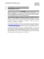
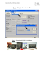
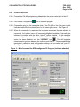
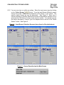
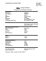
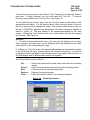
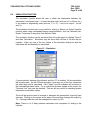
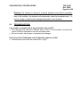
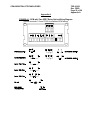
CONAX BUFFALO TECHNOLOGIES
TSD 43.021
Rev. ORIG
Page 1 of 28
INSTALLATION AND MAINTENANCE MANUAL
FOR
CONAX BUFFALO
PC PROGRAMMABLE INDICATORS
“SPM” SERIES
CONAX BUFFALO TECHNOLOGIES
TSD 43.021
Rev. ORIG
Page 2 of 28
TABLE OF CONTENTS
SECTION
DESCRIPTION
PAGE
1.0
SCOPE
3
2.0
APPLICABLE DOCUMENTS
3
3.0
GENERAL DESCRIPTION AND
STANDARD FEATURES
3
4.0
SPECIFICATIONS
4
5.0
INSTALLATION
5
6.0
SOFTWARE INSTALLATION AND
CONFIGURATION
6
7.0
TRIMMING FUNCTION
21
8.0
SIMULATION FUNCTION
23
9.0
TROUBLESHOOTING
24
A
WIRING DIAGRAMS
25
B
PROGRAMMING SOFTWARE
28
APPENDIX
CONAX BUFFALO TECHNOLOGIES
1.0
TSD 43.021
Rev. ORIG
Page 3 of 28
SCOPE
This manual provides instructions on setup and use of Conax Buffalo
Technologies, PC- Programmable, SPM-4XX series Indicators.
2.0
APPLICABLE DOCUMENTS
2.1
Conax Buffalo Technologies (CBT) Sales Order.
2.2
Customer Purchase Order (specified in CBT Sales Order).
2.3
Either CBT Part Number 80-0034-001 (CDROM) or 80-0034-002 (3.5” diskettes),
Programming Software for PC-Programmable Indicators.
2.4
CBT Part Number 318997-001, Programmable Adaptor Cable, Model No. PA400.
2.5
CBT Drawing No. 10-0554; Indicator, Model No. SPM-400.
3.0
GENERAL DESCRIPTION AND STANDARD FEATURES
The SPM-4XX indicators are state-of-the-art, micro-processor and flash memory
based, high performance indicators. All models can be fully configured using the
user friendly configuration software. This unique and user-friendly software
facilitates logical and speedy setup of the indicators using only a Windows® PC,
RS-232 serial port and the PA-400 serial adapter cable. No calibrator or meter is
required.
The SPM indicators are supplied with input and output reference parameters fully
factory calibrated. For actual operation all that is required is to perform the
simple and easy configuration procedure.
CONAX BUFFALO TECHNOLOGIES
4.0
SPECIFICATIONS
4.1
SENSOR INPUT TYPES
TSD 43.021
Rev. ORIG
Page 4 of 28
THERMOCOUPLE: Most standard types and all special types using customer
defined tables and polynomials.
RTD (2, 3 or 4 wire configuration): Platinum (e.g. Pt-100), Nickel, Copper, and
other RTDs (includes Callander-Van-Dusen and custom sensor linearization with
user defined tables and polynomials up to 10th order).
DCmV: -120 to 120 mV
DCmA: -25 to 25 mA
Resistance: 3-wire potentiometer up to 20KΩ or 200Ω standard
4.2
4.3
GENERAL SPECIFICATIONS
MINIMUM RANGE:
2 mV, limited mostly by input signal quality.
SUPPLY VOLTAGE:
115VAC, 230VAC or 24VDC±10%
OPERATION TEMPERATURE:
-20 to 70°C.
STORAGE TEMPERATURE:
-55 to 125°C.
HUMIDITY:
0-95% RH, non-condensing.
RESPONSE TIME:
0.3 seconds to 90% of reading (>3 updates per
second).
DAMPING FACTOR:
Programmable 0.0 to 64.0 seconds, or
0 – 120% of input range, using software
interface.
PERFORMANCE SPECIFICATIONS
OUTPUT (D/A) LINEARITY:
Better than 0.005% of output span (mV input)
SENSOR LINEARIZATION:
Better than 0.1°C for RTD. Better than 0.2°C
for Thermocouple over full span or < 0.1˚C
over ≤ 200˚C span.
LONG TERM STABILITY:
Better than ±0.5% of span for 12 months
CONAX BUFFALO TECHNOLOGIES
TEMPERATURE STABILITY:
TSD 43.021
Rev. ORIG
Page 5 of 28
Better than 0.012%/˚C of span
COLD JUNCTION COMPENSATION:
Automatically corrected to within ±0.5°C for all
T/C types.
4.4
OUTPUT RESOLUTION:
(optional) 12-bit D/A with 0.025% of span
I/O ISOLATION:
2000 VDC or peak AC (input/output/supply)
RFI PROTECTION:
Better than 0.5% effect of span at 20 – 1000
MHz and at field strength of 20 V/m. CE
marked.
INTERNAL OPTIONS
ANALOG OUTPUT:
4-20mA retransmission
SENSOR POWER SUPPLY:
28 VDC nominal, 25 mA MAX
RELAY OUTPUTS:
up to 6 dry contacts (SPST)
TRI-COLOR DISPLAY:
Numeric color changed based on trip setpoints
5.0
INSTALLATION
5.1
Mounting
The SPM is mounted through a 1.772” x 3.602” (45 x 92 mm) opening in a panel.
Screws and brackets are supplied that tighten the meter to the panel from the
backside (pressing against the faceplate).
5.2
Wiring
Removable terminals are provided on the back of the meter to wire the meter.
Wiring diagrams can be found in Appendix A at the end of this document.
CONAX BUFFALO TECHNOLOGIES
6.0
SOFTWARE INSTALLATION AND CONFIGURATION
6.1
SOFTWARE INSTALLATION
TSD 43.021
Rev. ORIG
Page 6 of 28
CAUTION
BEFORE INSTALLING THE NEW CONFIGURATION SOFTWARE, IT IS
ALWAYS ADVISABLE TO CLOSE ALL OTHER APPLICATIONS INCLUDING
VIRUS SCANNERS AND OFFICE SUITES. FAILURE TO DO SO MAY RESULT
IN THE CORRUPTION OF CERTAIN COMMON FILES.
The configuration software is provided on either one CDROM or two 3.5”
diskettes. It may be installed on any Windows® operating systems. To install,
insert the provided media into the proper drive on your computer and run either
“setup.exe” (floppies) or “cspm481.exe” (CDROM).
Follow the onscreen
instructions to complete the installation.
The configuration software may also be freely downloaded from Conax’s web site
at http://www.conaxbuffalo.com. Once at Conax’s site, navigate to “Technical
Data” and browse the page to find the latest version referencing SPM indicators.
For proper communication using your programming adapter, you must first
identify and set the serial port to which it is connected. After the proper serial
port is identified, open the SPMconfigurator32 software. From the menu bar,
select the “Options” menu, click on “Communication” and enter the correct COM
port designation from the pull-down menu. See Figure 1.
CONAX BUFFALO TECHNOLOGIES
TSD 43.021
Rev. ORIG
Page 7 of 28
Figure 1 – Setting the Communications Port
1
2
Figure 2 – Connecting the PA-400 to the Indicator
PA-400 Plug
CONAX BUFFALO TECHNOLOGIES
6.2
TSD 43.021
Rev. ORIG
Page 8 of 28
CONFIGURATION
6.2.1 Connect the PA-400 programming adapter into the proper serial port of the PC.
6.2.2 Click on the Configuration
icon to start the program.
6.2.3 Connect the plug on the transmitter side of the PA-400 to the 6-pin jack on the
indicator, behind the front bezel (lens) in the lower-right corner. See Figure 2.
6.2.4 When the connection is made and the software recognizes that the indicator is
connected, the toolbar icons will become highlighted (enabled). Normally, the
software is installed with the “Auto Upload” option enabled. In this case the
current configuration stored in the indicator will be loaded into the software. If the
. This will begin the
option has been disabled, click the “UPLOAD” icon
communication process between the indicator and the PC. Once completed, the
transmitter’s calibration and configuration settings will be loaded into your PC.
See Figure 3.
Figure 3 – Main Screen of the SPMconfigurator32 Program (Indicator attached)
CONAX BUFFALO TECHNOLOGIES
TSD 43.021
Rev. ORIG
Page 9 of 28
6.2.5 You can now view or modify any setting. Select the input sensor type by clicking
on the “Select Sensor”
button. From the Input Sensor Selection screen
choose the proper “TAB” that corresponds to the sensor of your choice. The
specific sensor screen will now be presented. See Figure 4. Enter one of
several methods to precisely describe the sensor’s temperature reactance curve
and press the OK button to return to the previous screen. You should now see
the sensor described in “Sensor Type” box adjacent and to the left of the “Select
Sensor” button. See Figure 5.
Figure 4 – Input Sensor Selection Screens (view of each of the tab buttons)
Figure 5 – Sensor Described on the Main Screen
CONAX BUFFALO TECHNOLOGIES
TSD 43.021
Rev. ORIG
Page 10 of 28
6.2.6 Units. Next, verify or select the “Engineering Units”. If appropriate, open the
pull-down menu and select the appropriate units of either °F, °C or °K. See
Figure 6.
Figure 6 – Selection of Engineering Units
6.2.7 Range. TAB or click to the next box which is “Zero”. Just to the right of the
“Zero” box in purple text is the range of allowable values for the selected sensor.
Enter the “Zero” value to define the specific input low. Next TAB or click to the
“Full Scale” box. Enter the “Full Scale” value that defines the transmitter’s
high input range. See Figure 7.
Figure 7 – Input of Sensor Range
6.2.8 Display scaling. The display can scale the input parameters to any reasonable
engineering scale by putting the corresponding “Zero” and “Full Scale” scaled
values in the Display unit fields. The displayed value will be the real sensor value
scaled to the entered Display units. This section is not normally required for
normal thermocouples and RTDs, and it is normally disabled when these sensor
types are selected. It can be enabled, if desired, by selecting “Options”,
“General” and checking the “Enable Scaling for Temperature Sensors” box.
6.2.9 Decimal point. Use the pull-down box to choose where you would like the
decimal point to display on the indicator. You can display no decimal/fractional
degrees (“####.”) up to three decimal/fractional degrees (#.###). The number of
CONAX BUFFALO TECHNOLOGIES
TSD 43.021
Rev. ORIG
Page 11 of 28
digits that can be displayed before the decimal point depend on the display
capability of the meter (i.e. 4 to 6 digits in total).
6.2.10 Sensor failure (Open) or Burnout. This feature is only relevant on SPM units
with the Analog Output (retransmission) option. An open sensor will cause the
display to read “EEEEE” for this error mode. TAB to the “Burnout” mode and
select from the pull down menu either “Upscale” or “Downscale”.
6.2.11 Next, TAB to the “Line Frequency” field and select from the pull-down menu
either “50 Hz” or “60 Hz” as appropriate for the installation site line frequency.
6.2.12 Next Click on the
button to have the computer calculate and
enter the normally optimal values for the damping factor and the damping filter
band. See Figure 8. See Paragraph 7.4 for more detailed information on the
filtering function.
Figure 8 – Input Filtering
Figure 9 – Device Status, Communication & Display
CONAX BUFFALO TECHNOLOGIES
TSD 43.021
Rev. ORIG
Page 12 of 28
6.2.13 Next, TAB over to the I.D. Tag: and type in up to 8 alpha-numeric characters for
a description to be saved in the transmitter’s memory. You may do the same
for the Job: and Message: boxes and type in information in these boxes.
Message will store up to 16 characters. See Figure 9.
6.2.14 Download to the indicator. Once you have verified all the information on the
screen, you are ready to download the information to the indicator. Click the
“Download” button
to send the information to the indicator. Ensure that
the serial adapter cable remains in place until the status bar (bottom-left of
program window) says that it has completed successfully. All the information is
stored in non-volatile memory in the indicator and will be remembered even
after no power has been applied to the indicator for some time.
6.2.15 Verify the information.
If you desire, You may verify the memory contents by
clicking on the verify
icon, or you may enable the “Auto Verify” function by
selecting “Option” and “General” from the top menu, checking the
corresponding box in the option screen and clicking “OK”. In the verification
process the settings are uploaded from the indicator and are compared to the
current settings. If they are not identical, a message box will appear. In this
case, simply repeat the download and verification process.
6.3
OTHER FEATURES, OPTIONS AND SETTINGS
6.3.1 All SPM indicators contain several alphanumeric fields, which may be used to
specifically identify that individual unit. These include:
I.D. Tag:
Job:
Message:
Up to 8 alphanumeric characters
Up to 8 alphanumeric characters
Up to 16 alphanumeric characters
These fields can be changed or modified at any time. Just click on the
appropriate field and enter the text. To conclude and save this information, click
on the “DOWNLOAD”
icon. The information will be downloaded and
stored in the indicator’s non-volatile memory. Indicator configuration information
can be retrieved at any time just by clicking on the “UPLOAD”
icon.
6.3.2 The indicator may be purchased with several added features, such as analog
output, alarm set points, function keys, communications and multi-color display.
To configure these options, when available, click on the “Select Feature” button.
The Input Feature Selection screen will appear. Only the available features will
be highlighted. An example of one of these screens is shown in Figure 10.
CONAX BUFFALO TECHNOLOGIES
TSD 43.021
Rev. ORIG
Page 13 of 28
Figure 10 – Example Input Feature Selection Screen
6.3.2.1
Set points. This screen controls the triggering of two relays. First, determine
and mark the direction of the alarm activation as being either a “High” or
“Low” alarm. You can enter either “Trip ON” and “Trip OFF” values or “Trip
Point” and “Dead Band”. The difference between Trip ON and OFF is equal
to the dead band (or hysteresis). Select the desired relay state for the alarm
condition as being either closed in alarm state (normal) or open (inverse
operation). Click “Apply” to save the settings and click “OK” to exit back to
the main screen if no other options need to be set. See Figure 10.
6.3.2.2
Display color. This screen controls the color for the various alarm conditions.
The column designated as “Alarm Status” indicates the various possible
alarm conditions resulting from the set point settings. Click on the color bars
under the “Display Color” column to change the color bar between red, green
or yellow to indicate that alarm condition color. Click “Apply” to save the
settings and click “OK” to exit back to the main screen if no other options
need to be set.
6.3.3 Saving Configuration Information. Each indicator configuration may be saved
into a standard file. This information may be used for future references, reloading, archiving, statistical comparative analysis, and records.
To SAVE, click on the “DISKETTE”
icon in the tool bar and specify a file
name and directory location to which the file is to be saved.
CONAX BUFFALO TECHNOLOGIES
TSD 43.021
Rev. ORIG
Page 14 of 28
6.3.4 You can enable another toolbar icon that can configure several indicators with
the same settings. To do so, click “Options” and “General” from the top menu of
the main screen. Enable the “Regeneration Enable” option and click “OK”. To
configure a new indicator with the preloaded settings, click the regeneration icon,
on the icon bar of the main screen. The computer will automatically upload
the calibration parameters, calculate the proper configuration parameters and
download them into the indicator’s non-volatile memory.
6.3.5 Printing Configuration and Calibration Information. Click on the “PRINTER”
icon on the tool bar to initiate the printing of the indicator’s configuration and
calibration information. The report will include the values of the unit’s own input
and output calibration reference codes, configuration reference codes, current
time and date, the date of last configuration, and the date of the last calibration.
The printed information can provide invaluable data in the system’s performance
research, error corrections, and “before” and “after” analysis. See Table 1.
CONAX BUFFALO TECHNOLOGIES
TSD 43.021
Rev. ORIG
Page 15 of 28
Table 1 – Example Printout
Configuration and Calibration Information
Device Status
Unit Type:
Serial Number:
Tag:
Message:
Job:
PO Number:
PO Date:
Last Configuration Date:
SPM-400
DEMO133
970911
Product Intake
Chiller
971210MES
Wed, December 17, 1997
Fri, January 16, 1998
Sensor Type
Thermocouple, type K, Standard
Mode, Single Input
Input Range and Setup Option
Engineering Units:
Zero:
Full Scale:
Burnout:
Line Frequency:
Fahrenheit
0.00
500.00
Upscale
60 Hz
Filter
Damping:
Band:
15 sec.
0.44%
Calibration References
Output 4mA:
Output 20mA:
Input mV:
Input Ohms:
CJ Temperature:
1782
8948
91.289
301.023
296.768
Last Calibration Date:
Device Program I.D. :
Wed, November 19, 1997
31977.2
Printed on: Friday, January 16, 1998, 12:06:17
CONAX BUFFALO TECHNOLOGIES
6.4
TSD 43.021
Rev. ORIG
Page 16 of 28
INPUT FILTERING
Input filtering is of great importance in measurement application with a low level
signal. The effect of low pass filtering is to average out small transients of the
input parameter resulting from process and sensor noise, as well as externally
generated electrical noises. To overcome the sluggish response, associated with
long filter settings, the indicator uses a Selective Filtering technique. This
method allows the transmitter to achieve a fast response for significant variation,
yet to provide a stable, smooth and noise free output.
6.4.1 Damping Factor
The Damping Factor provides a measure of the time (in seconds) over which
the input signal will be averaged. The greater the Damping Factor, the
smoother the output and the slower the measurement display response time.
Selective Filtering implies that Damping is only applied over a limited input
Band around the input levels where noise is most likely to be found. This is the
Filter Band.
6.4.2 Damping Filter Band
The Filter Band is defined as the band (in % of the input span) over which
Damping is applied. A 1% Band for a transmitter with a measurement input span
of 500° C means that Damping will apply to input variations of 0.5° C or less.
However, changes in the input of greater than 0.5° C will be directly reflected in
the indicator’s output without a delay.
Since noise levels do not vary largely between most applications, it is sensible to
assume that wide input spans would require low band settings and narrow spans
would require large band settings. The Configuration software provides for a
calculated optimal filter setting suitable for the majority of applications,
accounting for the specific transmitter input span.
To enable the automatic application of this function, simply click on the “Set to
button. The settings may be changed at any time for
Optimal”
applications where a high level of noise is known to exist, or in a slow responding
system where a very smooth output signal is imperative.
CONAX BUFFALO TECHNOLOGIES
6.5
TSD 43.021
Rev. ORIG
Page 17 of 28
USER DEFINED TABLES
For applications where the input is non-standard and non-linear, a User Defined
Table (UDT) provides a simple and convenient way of linearizing an input to a
known set of datum.
Two methods are used for creating “User Defined Tables”. One is for
temperature sensors such as thermocouples and RTDs. The other is for inputs
such as mV, Volts, mA, resistance, and potentiometers.
The tables must be made in simple text (ASCII) files. These text files may be
written in, or transferred to, any standard text editor. Lines containing notes,
memos, comments, and descriptions must be preceded with an asterisk (*). The
asterisk signifies to the software that this line is not a part of the conversion table.
No letters, symbols or other characters are allowed in the data. See Table 2. It
is a good practice to include description, reference and other application notes in
the heading of the table proceded by asterisks.
It is highly suggested, although not required, that you use at least 141 points to
describe the sensor in the application’s range. This will ensure that the software
closely matches the sensor’s actual output and reduce the linearization error.
It may also be useful to open up a special directory for storing such tables in
order to facilitate easy access in future use. We also recommend using a .tbl file
extension in order to distinguish these special files from others.
6.5.1 UDT for Thermocouples and RTDs.
The conversion table should be formatted to contain two columns of numerical
values only. No letters, symbols or other characters are allowed in non-remark
lines. The first column is designated as the input column and should list the
temperature values in °C in increasing order with identical increment values;
each subsequent number should be larger than the previous by the same
amount. The second column should be separated by a single space or TAB and
should list the corresponding sensor output values (mV for thermocouples and
Ohms for RTDs).
It is recommended to apply the simulator function (Reference Para. 8.0) in order
to verify that the input and output parameters correspond to the required values.
6.5.2 UDT for General Purpose Inputs
The first column should display the values of the actual sensor output in mV, mA,
Volts, Ohms or percent (%) for potentiometers. The second column should
display the corresponding values in engineering units. Display scaling, on the
main configuration screen, may also be applied to this table of engineering units.
CONAX BUFFALO TECHNOLOGIES
TSD 43.021
Rev. ORIG
Page 18 of 28
Table 2
*User defined table for
*IRt/c.xxx-K-80F/27C
*Minimum range -70 degrees Celsius
*Maximum range 200 degrees Celsius
*First column degrees Celsius
*Second Column mV
*Delta 10 degrees
*Use with Thermocouple Sensor Type, User defined table
*Created November 7, 1997
-70.00
-2.59
-60.00
-2.26
-50.00
-1.92
-40.00
-1.57
-30.00
-1.20
-20.00
-0.82
-10.00
-0.42
0.00
0.00
10.00
0.44
20.00
0.90
30.00
1.38
40.00
1.90
50.00
2.44
60.00
3.01
70.00
3.62
80.00
4.26
90.00
4.95
100.00
5.67
110.00
6.45
120.00
7.28
130.00
8.16
140.00
9.09
150.00
10.07
160.00
11.09
170.00
12.16
180.00
13.27
190.00
14.40
200.00
15.55
CONAX BUFFALO TECHNOLOGIES
TSD 43.021
Rev. ORIG
Page 19 of 28
Figure 11
6.5.3 Using the UDT. When configuring the sensor, select “User Defined Table” under
the “Mode” section (usually the bottom-right of the “Input Sensor Selection” screen).
A popup screen will appear asking for the “Minimum range” and “Maximum range”
to use of the tabular data within the table. This range must exist within the *.TBL
file, and it is highly suggested that a few values outside this range are also included
in the file. This will allow the program to more accurately model the sensor output.
In Figure 11, ”Conax-SP_C5.tbl” will be imported into the Configuration software
and will be used for the specific application.
SPEICAL CONSIDERATION
An indicator that has been configured with a UDT will require this table when you
upload and/or reconfigure the indicator. Keep this file handy for future use. It is
highly suggested that you save both the UDT and Configuration file to a portable
media such as a Floppy or CDROM for future reference and mark it accordingly.
6.5.4 CREATING A TABLE FROM A MATH FUNCTION
If your sensor’s transfer function can be described in a mathematical equation
(trigonometric, log, etc.), use a commercial spreadsheet program, such as Excel or
Lotus to generate a table using the restrictions described in Para 7.5. Use “COPY”
and “PASTE” or “Save as” commands to transfer the table section to any text
editor such as “Notepad” or directly to a text file. Edit the table and text according
to the above instructions to ensure that the table is formatted correctly and contains
enough data points.
6.5.5 APPLYING THE “USER DEFINED TABLE” FUNCTION (reference Figure 11)
a. When selecting the input sensor for the application, from the “Transfer Function”
or “Mode” selection box, select the “User Defined Table” button.
b. Enter the minimum and maximum table input range.
d. Enter the table’s complete file name or click “Browse…” to find it.
e. Select the “OK” button to apply the table to the application.
f. This table will be required during all future uploads and/or reconfigurations.
CONAX BUFFALO TECHNOLOGIES
6.6
TSD 43.021
Rev. ORIG
Page 20 of 28
CALLENDAR-VAN-DUSEN APPLICATIONS
The Callendar-Van-Dusen formula provides constants for a third order polynomial
equation, which then approximates the actual Pt-100 RTDs resistance to a high
degree of precision.
Of course, the specific RTD needs to be precisely
characterized by exact temperature testing, and the coefficients should then be
calculated. See Figure 12.
α
β
δ
Alpha is the nominal coefficient for the RTD, which, for most standard elements will
be in the vicinity of 0.00385 (DIN curve).
Beta is zero (0) for temperatures >0 °C. It is the significant constant for <0 °C
ranges.
Delta is the significant coefficient for the higher temperature ranges.
Figure 12 – RTD Callendar-Van-Dusen Entry
The minimum and maximum values are the temperatures within the values for
which the sensor was supposed to be defined and tested for. The units are always
in °C. If the sensor was tested and defined between -50°C and +450°C, you may
enter any values up to and including -50°C for the minimum value and +450°C for
the maximum value.
You MUST enter a value for Delta or else the program will request it. Typical
values will run in the order of 1.40 to 1.60 for 100 Ω (@ 0°C) elements. For units
with the 0.000385 curve, the typical values are in the order of 1.45 to 1.47.
Once you enter all of the numbers, the configuration software will generate the
linearization table for the particular range of the unit. Upon downloading, this table
will be entered into the transmitter’s memory.
CONAX BUFFALO TECHNOLOGIES
TSD 43.021
Rev. ORIG
Page 21 of 28
Please Note:
The calculated values may be verified by using the device in
simulation mode (Alt+S from the main screen) and seeing that the device indeed
provides the proper temperatures (and/or output values in mA) for the resistances
found by the element’s tests, or vice versa.
6.7
POLYNOMIAL FUNCTIONS
Some sensor outputs can be characterized by a non-linear transfer function of the
form shown in Equation 1. If the transfer function can be described using such a
multi-order polynomial (max 10th order), then the sensor’s output may be linearized
by the transmitter using “Polynomial” mode in the “Input Sensor Selection” screen.
When selected, an input screen, like that shown in Figure 13, will popup asking for
the coefficients to Equation 1 (shown below).
Equation 1 – Polynomial Input Feature
SensorOutput (t ) = A0 + A1t + A2t 2 + A3t 3 + K + A10t 10
Figure 13 – Polynomial Input Feature
7.0
Trimming
Realizing that some sensor or system outputs may vary from their ideal output
curves, the trimming function allows the user to fine-tune the SPM calibration to
match the specific sensor or system back to ideal conditions. The trimming function
is a smart substitute for common “zero” and “span” adjustments found on
transmitters.
CONAX BUFFALO TECHNOLOGIES
TSD 43.021
Rev. ORIG
Page 22 of 28
To enter the trimming screen, click “Device” then “Trimming” from the main screen’s
menu bar. To apply trimming, first, you must check the “Trim On”. To remove
trimming, simply uncheck the “Trim On” box. See Figure 14.
To trim either the zero and/or span, click the “UnLock” button at the bottom of the
appropriate scroll bar(s). You will now be able to either move the slider or click on
the up or down arrows to change the output. The trimmed value shown on the top
will say “<TRIM ON>” adjacent the temperature unit when trimming is applied as
shown in Figure 14. This also applies to the temperature readout on the main
screen. Clicking the “Lock” button under one or both sliders will hold the changed
trim value(s). See Figure 14.
NOTE(S):
1. To avoid potential adjustment errors, the zero may be adjusted at any input
value, however, the span may only be adjusted when the measured input value
exceeds 50% of the configured input range.
2. While in the “Trim On” mode, the trimming adjustments are downloaded instantly
to the SPM and the units’ display reflects the trimmed information. It should be
noted that the data displayed in the trimming screen may slightly differ from that of
the SPM display due to different filters used in the systems.
The control buttons work as follows:
OK ...............Saves and downloads the new setup and closes the trimming
screen
Cancel .........Restores the previous setup and closes the trimming screen
Hint..............A few words about the trimming function
Restore .......Restores the previous setup
Clear............Clears the trimmed values to non-trimmed operation
Figure 14 – Trimming Function
CONAX BUFFALO TECHNOLOGIES
8.0
TSD 43.021
Rev. ORIG
Page 23 of 28
SIMULATION FUNCTION
The simulation function allows the user to check the relationship between the
transmitter’s configured input – in basic electrical units (such as mV or Ohms, etc.)
to the scaled or engineering units (such as °F or °C) – and to its output – (in mA
and %).
The simulation function also is very useful for testing a “Sensor vs. Output” transfer
function when using nonstandard sensor transformations, such as Calender-VanDusen, Polynomial or any other User Defined Table.
The simulation function can be accessed from the main menu by clicking “Device”
and then “Simulation.” Simulation may be done while Off-line or On-line with an
indicator. Enter any one of the four values in the simulation dialog box and the
other three will automatically be calculated.
Figure 15 – Simulation
If communication between the indicator and the PC is enabled, On-line simulation
will be performed. As with Off-line simulation, enter any one of the four values and
the other three will be calculated. Click “Apply” and the indicator will be driven to
the indicated/calculated value. For a continuous dynamic update of the output, the
“Dynamic Link” box must be checked. This can be very useful for checking system
responses to calculated values.
The scroll bar may be used to increase or decrease the transmitter’s output by fixed
amounts. Clicking on the arrows at the ends of the scroll bar changes the output by
1%. Clicking inside the scroll bar changes the output by 10%.
Note: There is a 2-3 delay between calculation and completion of writing to the
indicator.
CONAX BUFFALO TECHNOLOGIES
TSD 43.021
Rev. ORIG
Page 24 of 28
Warning: The indicator is running in a special software mode while in simulation
mode. If you happen to lose communications before the normal software is written
back to the indicator, the indicator will continuously output the simulated value. To
restore, simply re-download the settings/configuration to the indicator.
9.0
TROUBLESHOOTING
I am unable to communicate to my transmitter from my PC?
• From the menu bar, select the “Options” menu, click on “Communication” and enter the
correct COM port designation from the pull-down menu.
• Exit and re-enter the program to implement the changes.
How do I print the Calibration and Configuration reports to a file?
• Install another printer with the same driver: “copy2”.
CONAX BUFFALO TECHNOLOGIES
TSD 43.021
Rev. ORIG
Page 25 of 28
Appendix A
Appendix A
FIGURE A1 - SPM with Two SPDT Relay Option Wiring Diagram
(ignore terminals 7-9 and 27-29 for standard SPM wiring)
CONAX BUFFALO TECHNOLOGIES
TSD 43.021
Rev. ORIG
Page 26 of 28
Appendix A
Figure A2 – SPM with two SPST Relay Option Wiring Diagram
CONAX BUFFALO TECHNOLOGIES
Figure A3 - SPM for AC Measurement Wiring Diagram
TSD 43.021
Rev. ORIG
Page 27 of 28
Appendix A
CONAX BUFFALO TECHNOLOGIES
TSD 43.021
Rev. ORIG
Page 28 of 28
Appendix B
APPENDIX B
PROGRAMMING SOFTWARE
MEDIA & MEDIA POCKET HERE
END OF DOCUMENT