1
E X T R O N E W S M AY / J U N E 1 9 9 9
Comb Filters:
NTSC Decoding Basics
by Steve Somers, V.P. Engineering
Adaptive Comb Filter
Decoders (Part 4)
This is the last installment of our
series on NTSC decoding basics, and
Y/C separation in particular.
Meanwhile the quest for high quality
decoders continues on into the sunset
of NTSC. The emphasis here is on
the first step in the process known as
Y/C (luma/chroma) separation since it
does represent the most crucial step in
realizing the full potential of the
transmission medium. The earlier
installments covered NTSC signal
creation, notch/bandpass filtering, and
line comb filters.
Implementation of high-speed digital
processing and low cost memory
components facilitated many improvements in Y/C separation. These strides
in decoding performance involve
decision-making, called adaption,
Composite
NTSC
based upon image content. Moreover,
having more image memory available
means that video processing can now
take place beyond the original 2D
boundaries (i.e. the information within
a picture field). Processing decisions
now extend into the temporal realm, or
from picture frame to picture frame.
This means more intelligence in Y/C
separation as subject matter moves
across the screen from frame to frame.
2D OR NOT 2D?
Since conventional (line type) comb
filters have problems handling diagonal
lines and vertical color changes, it
seems the first order of business would
be to tackle these tricky situations.
Remember that when processing
diagonal lines, succeeding luma (Y)
information is shifted in time and does
1-H
Delay
1-H
Delay
1
/2
1
/4
+
Y CHANNEL
1
/4
1
/2
1
/4
-
C CHANNEL
STEVE SOMERS
not properly cancel line-to-line or fieldto-field. This results in Y information
being interpreted as chroma (C) information. The outcome is “cross color”
or the rainbow effect in the region of
the diagonal lines. The vertical color
changes, which do not match in time at
the transition point, result in chroma
information being interpreted as Y
information. Hence, you see the
“hanging dots” at the color boundary.
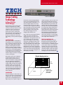
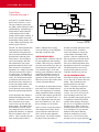
Now, suppose we take the two-line
comb design discussed previously
(see Figure 1). This design is
comparing data between two stored
lines and the incoming data. It utilizes
averaging to soften the transition
between colors. If we add a system
called a correlator, data between the
three lines can be tested before any
actual averaging or summation takes
place (see Figure 2). Here, if there is
significant correlation of data value
between Line 1 and Line 2, then CF= 0
and a difference between Line 2 and
Line 1 is used. But, if Line 2 and Line
3 correlate to a higher degree, CF= 1
and the difference between Line 2 and
Line 3 is used. If there is no correlation
1
/4
FIGURE 1. 2-LINE COMB FILTER
(continued on page 18–
See “Comb Filters”)
5