Download Emerson E2 Einstein User`s manual

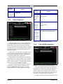
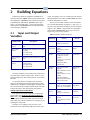
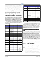
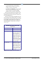
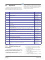
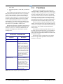
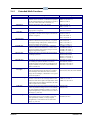
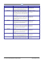
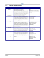
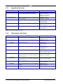
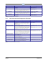
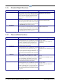
026-1620 Rev 0 09-15-05
E2 User’s Manual Supplement: Flexible Combiner
Programming
Computer Process Controls, Inc.
1640 Airport Road Suite #104
Kennesaw, GA 31044
Phone (770) 425-2724
Fax (770) 425-9319
ALL RIGHTS RESERVED
The information contained in this manual has been carefully checked and is believed
to be accurate. However, Computer Process Controls, Inc. assumes no responsibility
for any inaccuracies that may be contained herein. In no event will Computer Process
Controls, Inc. be liable for any direct, indirect, special, incidental, or consequential
damages resulting from any defect or omission in this manual, even if advised of the
possibility of such damages. In the interest of continued product development, Computer Process Controls, Inc. reserves the right to make improvements to this manual,
and the products described herein, at any time without notice or obligation.
Computer Process Controls, Inc. products may be covered by one or more of the following Computer Process Controls U.S. patents: 6360553, 6449968, 6378315,
6502409, 6779918, and Computer Process Controls Australian patent No. 775,199 November 4, 2004.
FCC COMPLIANCE NOTICE
This device complies with Part 15 of the FCC Rules. Operation is subject to the following two conditions: (1) this device may not cause harmful interference, and (2) this
device must accept any interference received, including interference that may cause
undesired operation.
CE COMPLIANCE NOTICE
Class A Product Information for Einstein, E2 Controllers:
The CPC Einstein and E2 controllers are Class A products. In a domestic environment
this product may cause radio interference in which case the user may be required to
take adequate measures. This covers:
•
All Einstein family product types: RX - Refrigeration Controller
(830-xxxx), BX - Building/HVAC Controller (831-xxxx), and all version models: (300, 400, 500).
•
All E2 family product types: RX - Refrigeration Controller (834-xxxx),
BX - Building/HVAC Controller (835-xxxx), CX- Convenience Store
Controller (836-xxxx), and all version models: (300, 400, 500).
Table of Contents
1 FLEXIBLE COMBINER .......................................................................................................................................... 1-1
1.1 OVERVIEW .................................................................................................................................................................
1.2 HOW IT WORKS .........................................................................................................................................................
1.2.1 Example..............................................................................................................................................................
1.3 INPUT AND OUTPUT ASSIGNMENT .............................................................................................................................
1.3.1 Programming the Inputs and Outputs................................................................................................................
1.3.1.1
1.3.1.2
1.3.1.3
1.3.1.4
1-1
1-1
1-1
1-1
1-2
Adding a Flexible Combiner Application................................................................................................................ 1-2
Flexible Combiner General Setup............................................................................................................................ 1-2
Inputs........................................................................................................................................................................ 1-3
Outputs..................................................................................................................................................................... 1-3
1.4 EQUATIONS ................................................................................................................................................................
1.4.1 Types of Equations and Where Equations are Entered .....................................................................................
1.4.2 Output Equations ...............................................................................................................................................
1.4.3 Delay Equations.................................................................................................................................................
1.4.4 Pulse Width Equations .......................................................................................................................................
1.5 ENGINEERING UNITS..................................................................................................................................................
1-3
1-4
1-4
1-5
1-5
1-6
2 BUILDING EQUATIONS ........................................................................................................................................ 2-1
2.1 INPUT AND OUTPUT VARIABLES ............................................................................................................................... 2-1
2.2 CONSTANTS ............................................................................................................................................................... 2-2
2.2.1 Constants and Engineering Units ...................................................................................................................... 2-2
2.2.2 Specifying a Constant’s Engineering Unit with Type Suffixes........................................................................... 2-3
2.2.3 Time Constants................................................................................................................................................... 2-3
2.3 OPERATORS ............................................................................................................................................................... 2-5
2.3.1 Multiple Operators and Parenthesis.................................................................................................................. 2-5
2.4 FUNCTIONS ................................................................................................................................................................ 2-6
2.4.1 Extended Math Functions .................................................................................................................................. 2-7
2.4.2 Extended Logical Functions............................................................................................................................... 2-9
2.4.3 Logarithm Functions........................................................................................................................................ 2-10
2.4.4 Trigonometry Functions................................................................................................................................... 2-10
2.4.5 Unit Conversion and Temperature Functions ................................................................................................. 2-11
2.4.6 Extended Digital Functions ............................................................................................................................. 2-12
2.4.7 Time and Date Functions................................................................................................................................. 2-12
2.4.8 IF Functions..................................................................................................................................................... 2-14
3 TESTING AND TROUBLESHOOTING EQUATIONS ....................................................................................... 3-1
3.1 CHECKING FOR ERRORS ............................................................................................................................................ 3-1
3.1.1 Equation Troubleshooting Tips.......................................................................................................................... 3-2
E2 User’s Manual Supplement: Flexible Combiner
Table of Contents • v
1
Flexible Combiner
1.1
Overview
The Flexible Combiner application, a new feature of
E2 versions 2.20 and above, is a highly advanced and versatile I/O control program used to combine multiple analog and digital input values using programmed equations
similar to those used in spreadsheets.
A Flexible Combiner application may have up to four
analog outputs and four digital outputs, each of whose values are determined by user-programmed equations that
mathematically combine up to eight analog inputs and
eight digital inputs. Equations used to calculate output values and time delays may use mathematical combinations
of any of the Flexible Combiner’s analog and digital
inputs, as well as numeric and named constants, operators,
functions, and even rudimentary if-then logic functions.
For control of digital outputs the Flexible Combiner
also supports separate equations that determine ON and
OFF delays. The Flexible Combiner may also be programmed to operate a digital output as a PWM (pulsewidth modulation) output. In this instance, the equation
written for a PWM output determines its period and pulse
width.
1.2
Outputs
The outputs of the Flexible Combiner are the real-time
results of the application’s equations. Each output’s value
is determined by the equation assigned to it in the Flexible
Combiner application.
Outputs of the Flexible Combiner application may be
tied to relay or analog output points on a CPC output
board, or they may be passed along to the inputs of other
E2 applications.
1.2.1
Example
Figure 1-1 shows a symbolic diagram of an example
Flexible Combiner application. In this diagram, there are
two equations shown: one for analog output AO1 and
another for digital output DO2.
The equation in AO1 is set up to make analog output
AO1 equal to the average value of the two analog inputs
AI1 and AI7. The equation adds these two values together
and then divides the result by two.
The equation in DO2 performs a logical AND function
on digital inputs DI1 through DI3. When all of these outputs are ON, the value of DO2 will be ON; otherwise, if
one or more of the inputs are OFF, DO2 will be off.
How It Works
A typical Flexible Combiner application consists of
three types of components: inputs, equations, and outputs.
Inputs
Inputs for a Flexible Combiner applications may be
sensor values from input points on a MultiFlex input board
or outputs from other software applications in the E2.
Inputs are the building blocks you will use to create the
control function you need.
A Flexible Combiner output may be configured with
up to eight analog inputs and eight digital inputs.
Figure 1-1 - Flexible Combiner Control Diagram
Equations
1.3 Input and Output
Assignment
Equations are used to combine or otherwise mathematically alter one or more inputs from the Flexible Combiner
to create an output that performs a desired function. Each
output has its own equation (a string of characters up to 80
characters in length) that the E2 “parses,” or decodes, to
determine the output’s value.
The first step in setting up a Flexible Combiner is configuring the application’s inputs.
Equations must be entered by the user and require
some basic knowledge of the E2’s scripting language,
which is further explained in this section of the manual.
The first question that must be answered before input
assignment can begin is “What do I want the Flexible
Combiner to do?” Will it choose the highest value from a
Overview
Overview • 1-1
series of temperature sensors? Will it calculate enthalpy
from temperature and humidity sensors? Will it read a set
of proofs and turn an output ON if more than half of them
fail?
Setup
When you have determined this, make a note of the
following:
• How many inputs of each type you will need (analog and digital)
• How many outputs of each type you will need (analog and digital)
• The types of analog inputs that will be used (temperature, pressure, etc.)
• For analog outputs, the range of values you want
each output to vary between (0-5V, 0-10V, 1-5V,
etc.)
Figure 1-2 - Flexible Combiner General Setup
• For digital outputs, whether you want each output
to be a simple ON/OFF digital output or a one-shot
output.
The first screen of the Flexible Combiner is where you
will set up the general parameters required to further
define the application’s functions.
The next step is to assign all the inputs and outputs to
the numbered input and output slots in the Flexible Combiner application.
1.3.1
Programming the Inputs
and Outputs
1.3.1.1
Adding a Flexible Combiner
Application
If you haven’t added a Flexible Combiner application
yet, you will need to create it in the E2’s Add Application
screen.
1.
Press I to access the Add Application
screen.
2.
With the cursor highlighting the Type field, press
D and choose “Flexible Combiner” from the
Look-Up Table. Note: If Flexible Combiner does
not appear in this list, it may be because your E2
is not version 2.20 or higher.
3.
Enter the number of Flexible Combiners you
wish to add in the “How many?” field.
4.
Press > to add the new applications.
5.
When the E2 asks “Do you wish to edit the new
applications now?” press . The E2 will take
you to the first setup screen of the application you
added (or, if you added multiple applications, it
will take you to the first application you added).
1.3.1.2
Flexible Combiner General
1-2 • E2 User’s Manual Supplement: Flexible Combiner
Name
Enter a short description of the Flexible Combiner’s
function in the Name field.
Num of AI
Enter the number of analog inputs the Flexible Combiner will use in this field.
Num of AO
Enter the number of analog outputs the Flexible Combiner will use in this field.
Num of DI
Enter the number of digital inputs the Flexible Combiner will use in this field.
Num of DO
Enter the number of digital outputs the Flexible Combiner will use in this field.
Show Eq Line 2
Each output in the Flexible Combiner has two lines of
40 characters each that may be used to enter its equation.
Since an equation rarely exceeds 40 characters, it is usually safe to hide the second line from display to make the
screen easier to read. This will be explained in further
detail in Section 1.4.1; for now, leave this field set to NO.
DO1-DO8 Type
The eight DO1-DO8 Type fields are used to specify
whether each digital output will be a simple ON/OFF digital output or a one-shot pulse output. Choose the desired
output type here.
026-1620 Rev 0 09-15-05
DO1-DO8 Trigger
If any of the DO1-DO8 Type fields were set up as oneshot outputs, choose the method the Flexible Combiner
will use to generate pulses. The choices are:
• Edge - Pulse is generated when the application transitions the output from OFF to ON.
of each input you defined (AI1-AI8 and DI1-DI8). These
names are the ones that are used when building equations.
When finished, press B to proceed to the Outputs
screen.
1.3.1.4
Outputs
• Inv Edge - Pulse is generated when the application
transitions the output from ON to OFF.
• Both Edge - Pulse is generated every time a state
transition occurs, whether it is OFF to ON or ON to
OFF.
Press B to proceed to the Inputs screen.
1.3.1.3
Inputs
Figure 1-4 - Flexible Combiner Outputs
The Outputs screen will show the output definitions for
the number of analog and digital outputs you specified in
Screen 1: General.
Figure 1-3 - Flexible Combiner Inputs
The Inputs screen will show the input definitions for
the number of analog and digital inputs you specified in
Screen 1: General.
The default input format is “Controller:Application:Output.” If you wish to use the output from another
E2 application as an input for the Flexible Combiner application, use the Look-Up Table (D) to select the controller, application name, and output name for each field in
the definition.
If you want an input to be a board and point address
from a MultiFlex input board, press C to change
the I/O format, and select from the menu to change the
format to Board and Point. Then, enter the board and point
address of the input point in each field.
NOTE: If a point you enter in this manner has not been
configured yet from the Input Summary screen, you will
need to do so before entering its board and point address
here. Refer to the E2 User’s Manual (CPC P/N 026-1610)
for more details.
Once all inputs are defined, make a note of the names
Equations
The default output format is “Controller: Application:
Input.” If you wish to use the input of another E2 application as the destination for a Flexible Combiner’s output
value, use the Look-Up Table (D) to select the controller, application name, and input name for each field in
the definition.
If you want an output to be a board and point address
from a MultiFlex output board, press C to change
the I/O format, and select from the menu to change the
format to Board and Point. Then, enter the board and point
address of the relay or analog point in each field.
ON DELAY and OFF DELAY
Each digital output will have two corresponding outputs, one for its on delay and one for its off delay. It is not
necessary to configure these outputs. They are only there
so the value of the on and off delays may be logged, used
in generic alarm control, and presented in status screens.
Once all inputs and outputs are configured, you will be
ready to complete the Flexible Combiner programming by
building equations.
1.4
Equations
The value of each output in a Flexible Combiner application is determined by its own equation, which usually
takes the values of one or more inputs and performs a
Equations • 1-3
mathematical operation or function on them to yield a single numerical value or digital state.
1.4.2
Output Equations
When entering an equation, you must follow a strict
format so that the E2 can properly understand and use the
equation. This section will explain how to build equations
in detail.
1.4.1
Types of Equations and
Where Equations are Entered
There are three different screens in the Flexible Combiner setup for output equations.
• Screen 4, the Output Eq screen, is where equations
that determine the output’s value are entered.
• Screen 5, the Delay Eq screen, is only visible if digital outputs are present. Equations that determine
the ON and OFF delays for digital outputs are
entered in this screen.
• Screen 6, the PW Eq screen, is only visible if one or
more digital outputs have been set up as “one-shot”
outputs. Equations that determine the pulse width
and period are entered in this screen.
Each of these screens lists the application outputs that
apply to it along with a 40-character field where the equation must be entered.
Section 2, Building Equations, provides a detailed
explanation of equation syntax in the Flexible Combiner
application.
Using the Second Line
If the “Show Eq Line 2” field is set to “Yes” in Screen
1, a “Line 2” field will be directly underneath each equation to expand the total equation size to 80 characters. If an
equation takes more than 40 characters to write, simply
write the first 40 characters in the first line and write the
remaining ones in the second line as if it were an extension
of the first line.
You can split variable names, constants, etc. between
the two lines with no problem. For example, if while writing an equation you have only two spaces left at the end of
line 1 and you must write the variable name “AO3,” simply write “AO” in the last two spaces and the “3” as the
first character of line two. When E2 parses the equation, it
will push line 1 and line 2 together into one long string,
and it will recognize the variable name as AO3.
Figure 1-5 - Flexible Combiner Output Equations
Screen 4 of the Flexible Combiner setup screens is
where equations that determine the output’s value are
entered. An output equation typically involves using mathematical operators or functions to combine or compare one
or more analog or digital outputs to yield a new output
result. Table 1-1 gives some useful examples of sensor
control applications used in refrigeration/HVAC applications and the equations used to achieve them. See Section
2, Building Equations, for a more detailed explanation of
equation components and functions.
Desired
Function
Equation
Averaging
three temperature sensors
AI1 through
AI3, and passing the result
to AO4.
AO4:
AVG(AI1,AI2,AI3)
Turn on an
exhaust fan at
DO2 when a
temperature
AI1 rises
above 120°F,
and turn it off
again when
the temperature falls
below 100°F.
DO2:
CUTINOUT(AI1,120DF,100DF,DO2)
Table 1-1 - Commonly Used Equation Examples
1-4 • E2 User’s Manual Supplement: Flexible Combiner
026-1620 Rev 0 09-15-05
tions.
Desired
Function
Equation
AND combination of digital inputs DI1
through DI8
DO1:
AND(DI1:DI8)
Table 1-1 - Commonly Used Equation Examples
1.4.3
Delay Equations
Figure 1-6 - Flexible Combiner Delay Equations
The digital outputs of a Flex Combiner application
have optional equations that can be used to program ON
and OFF delays. If the outputs are directly controlling
devices, ON and OFF delays can help minimize switching
by turning the output ON or OFF only when the equation
result that caused the transition remains in that state for
longer than the delay.
Desired
Function
Equation
Output DO1
has a 60 second ON delay
and a 60 second OFF
delay
DO1 OFF Delay:
60
DO2 OFF Delay:
60
Output DO2
has a 90minute ON
delay and a
90-minute
OFF delay.
DO2 OFF Delay
01:30
DO2: OFF Delay
01:30
Output DO3
uses a 5
minute delay
between the
hours of 9
p.m. and midnight, and a 3
minute delay
otherwise.
DO3:
IF(TIME()>9:00p,00:05:00,00:03:00)
Table 1-2 - Commonly Used Equation Examples
1.4.4
Pulse Width Equations
In other words, if an OFF delay is 30 seconds, and the
result of the input equation transitions from ON to OFF,
the result must remain OFF for thirty seconds before its
corresponding output actually changes state.
Delay equations do not actually have to be equations.
Most commonly, they will be constants. However, a delay
equation can be any mathematical expression (including
inputs, constants, operators, or functions) that results in an
analog value representing number of seconds.
If you have digital outputs and would like to use ON
and OFF delays, enter constants or equations in these
fields. See Section 2, Building Equations, for a more
detailed explanation of equation components and func-
Figure 1-7 - Flexible Combiner Pulse Width Equations
If one or more digital inputs have been configured to
be “One Shot” type outputs, the width of the ON pulse is
determined by the value of the Pulse Width equations.
When a one-shot output is called to be ON, the Flex Combiner will run this equation and use the resulting value as
the number of seconds the output will pulse ON.
Like delay equations, pulse width equations most com-
Equations
Equations • 1-5
monly will only be constant values, since there is usually
little need for variance in one-shot pulse width. However,
a delay equation can be any mathematical expression
(including inputs, constants, operators, or functions) that
results in an analog value representing number of seconds.
Desired
Function
Equation
5 second
pulse on DO1
DO1 PulseWidth:
5
2 minute
pulse on DO2
DO2 PulseWidth
00:02
15 second
pulse width
on DO3
unless the current time is
before 8 a.m.,
in which case
the pulse
width is 10
seconds
DO3 PulseWidth
IF((TIME()<08:00a)=TRUE,15,10)
For outputs, setting an engineering unit determines
how it is displayed in the Flex Combiner status screen. If a
unit is chosen for an output that is different from the
default engineering unit of the same type used by the E2 in
General Controller Info, the chosen type is substituted for
the default type on this screen only.
In other words, if AO1 is set to display in DF in the
Flexible Combiner cell but the default temperature unit for
the E2 is in DC, the output value will only be displayed in
DF on the Flex Combiner status screen — everywhere else
(including the Flex Combiner Summary Screen) it will
display in DC.
Table 1-3 - Commonly Used Equation Examples
1.5
Engineering Units
Figure 1-8 - Engineering Units
The engineering units used for each analog input and
output must be defined in Screen 7 of the Flexible Combiner setup screens: the Eng Units screen.
The units chosen for inputs are particularly important
in determining how the value will be scaled and used in
equations (see Section 2.2.1, Constants and Engineering
Units).
1-6 • E2 User’s Manual Supplement: Flexible Combiner
026-1620 Rev 0 09-15-05
2
Building Equations
Equations are made up of different combinations of
four major elements: inputs, defined in the Flexible Combiner application, constants such as numerical values used
in mathematical computations, operators such as plus
signs (+) or greater than signs (>) used to perform basic
math functions, and functions such as if-then statements
or boolean logic (AND/OR).
2.1 Input and Output
Variables
of AI1, the equation “AI1+10” would be incorrect because
this would add 10 to the value of AI in Celsius, since E2’s
SI unit for temperature is Celsius.
The way to correct this would be convert the number
10 to an equivalent number of degrees C (“AI1+5.6”), or
else use a type suffix so the E2 knows you want to add 10
degrees (“AI1+10DDF”). Type suffixes are explained in
further detail in Section 2.2.2, Specifying a Constant’s
Engineering Unit with Type Suffixes.
Table 2-2 lists the SI units used by E2:
Input Type
Variable Name
Description
AIx (x=input
number)
The analog value of input AIx, in SI
units
DIx (x=input
number)
The digital state of input DIx, converted
to analog:
1.0 if input is ON
0.0 if input is OFF
AOx (x=output
number)
The analog value of output AOx, in SI
units
DOx (x=output
number)
The digital state of output DOx, converted to analog:
1.0 if input is ON
0.0 if input is OFF
Table 2-1 - Input and Output Variable Names
Analog Input Values and SI Units
The value of an AI input will always be equal to the
current input value in the E2’s internal standard (SI)
units. This is important to remember because any mathematical operations that involve this value will use its SI
units, which may cause the equation to be wrong if you are
assuming the wrong units.
Example: AI1 is reading a value of 212°F. If you
wanted to write an equation that added 10°F to the value
Input and Output Variables
SI Unit
Temperature
degrees Fahrenheit (DF)
degrees Celsius (DC)
degrees C (DC)
Change in
Temperature
delta degrees Fahrenheit
(DDF)
delta degrees Celsius
(DDC)
delta degrees C
(DDC)
Pressure
inches of water (INW)
centimeters of water
(CMW)
pounds per sq. inch (PSI)
bars (BAR)
kilopascals (KPA)
pascals (PA)
pascals (PA)
Change in
Pressure
delta inches of water
(DINW)
delta centimeters of water
(DCMW)
delta pounds per sq. inch
(DPSI)
delta bars (DBAR)
delta kilopascals (DKPA)
delta pascals (DPA)
delta pascals
(DPA)
Air Velocity
feet per minute (FPM)
meters per minute (MPM)
meters per second (MPS)
meters per seconds (MPS)
Liquid
Velocity
gallons per minute
(GPM)
liters per second (LPS)
liters per second (LPS)
Volume
Flow
cubic feet per minute
(CFM)
cubic meters per second
(CMS)
cubic meters
per second
The most commonly used variables in an equation will
be the Flexible Combiner’s input values. These are represented in equations by their variable names, AI1-AI8 and
DI1-DI8.
To use input values in an equation, just enter their
names (AI for analog input or DI for digital input, and a
number from 1 through 8 corresponding to the input number). The E2 will look for input variable names and create
a link to the input’s value when parsing the equation.
Choices
Table 2-2 - SI Units for Analog Inputs
Input and Output Variables • 2-1
Input Type
Choices
SI Unit
Electrical
Current
amperes (A)
milliamperes (MA)
amperes (A)
Power Rate
watts (W)
kilowatts (KW)
watts (W)
Power Consumption
watt-hours (WH)
kilowatt-hours(KWH)
watt-hours
(WH)
Lumination
foot-candles (FTC)
lux (LUX)
lux (LUX)
Numeric
Constant
Types
Examples
Integers
7, -30
Whole numbers. A minus
sign in front will make it
negative.
Non-integers
1.0, -0.3,
3.14
Also called decimal or floating-point values. A minus
sign in front will make it
negative.
Exponential
Numbers
1.1E04
-4.5E-12
Large numbers can be
entered in exponential format. Format should be a
number with one significant
digit to the left of the decimal, followed by an E, then
followed by an integer that
corresponds to the power of
ten the number will be multiplied by. Example: 1.1E06
is 1.1 times 10 to the sixth
power, or 1,100,000.
Table 2-2 - SI Units for Analog Inputs
Digital Input Values and Analog Conversion
A digital input value is converted to a numerical value
when read into Flexible Combiner equations. A digital
input that is ON is treated as a unitless analog value of 1.0.
An OFF is treated as an analog value of 0.0. Logical operators such as AND, OR, XOR, and other functions typically used to combine digital inputs are all designed to
treat non-zero values as ONs for purposes of logic, and
zero values as OFFs.
A minus sign to the left of
the number makes the number negative. A minus sign
in between the E and the
exponent specifies a negative exponent.
EXAMPLE EQUATIONS: INPUTS
Equation
Description
AI4
The real-time value of AI4
AI1+AI2+AI3
Total sum of inputs AI1,
AI2, and AI3
Description
Table 2-4 - Numeric Constants
Table 2-3 - Equation Examples: Inputs
2.2
Constants
In addition to inputs, Flexible Combiner equations will
typically require use of constants. These can be either
numeric constants (entered as numbers and used as numbers), named consents (named strings that are parsed as
numbers), or time constants (times of day used in comparisons). Table 2-4 and Table 2-5 show the different
types of numeric and named constants.
Named
Constant
Description
PI
The value of pi (3.1415926535897)
TRUE
1.0 (to signify a logical TRUE)
FALSE
0.0 (to signify a logical FALSE)
ON
1.0 (to signify a logical ON)
OFF
0.0 (to signify a logical OFF)
Table 2-5 - Named Constants
2.2.1
Units
Constants and Engineering
Numerical and named constants are assumed to be
2-2 • E2 User’s Manual Supplement: Flexible Combiner
026-1620 Rev 0 09-15-05
unitless numbers. In other words, a “3.0” in an equation by
itself is not assumed to be 3.0 degrees or kilowatts. However, when used with a function or operator that involves
inputs of a specific type, the result of the operation or
function will use the inputs’ engineering unit designation.
For example, if analog input AI6 is a 0-100% humidity
sensor that is currently reading a humidity of 50%, the
result of the equation “AI6 / 5” will result in an output
value of 10%, even though the number 5 has no unit.
2.2.2
Specifying a Constant’s
Engineering Unit with Type Suffixes
Occasionally you may want to be specific about a constant’s engineering units. The equation parser supports the
use of a type suffix at the end of a constant to specify a
particular engineering unit. Table 2-1 lists all type suffixes
recognized by the Flexible Combiner’s equation parser.
Type suffixes must be placed directly after the constant
with no spaces in between the constant and the suffix (i.e.
75DF, not 75 DF).
Suffix
Unit
Suffix
Unit
DF
degrees F
%
percent
DC
degrees C
W
watts
DDF
delta degrees F
KW
kilowatts
delta degrees C
WH
watt-hours
°F per hour
KWH
kilowatt-hours
DFC
°C per hour
FTC
foot-candles
DFM
°F per minute
LUX
lux
(use this suffix
for offsets)
DFH
DCM
°C per minute
PPM
parts per million
INW
inches of water
OHM
ohms
CMW
cm of water
RPM
revolutions per
minute
PSI
pounds per
square inch
RPMM
RPM per minute
BAR
bars
DINW
differential
inches of water
KPA
kilopascals
DCMW
differential cm of
water
PA
pascals
DPSI
differential pressure in PSI
RH
relative humidity
DBAR
differential in
bars
FPM
feet per minute
DKPA
differential in
kilopascals
Table 2-1 - Type Suffixes for Flexible Combiner Constants
Constants
Unit
Suffix
Unit
MPM
meters per
minute
DPA
differential in
pascals
MPS
meters per second
GAL
gallons
GPM
gallons per
minute
L
liters
LPS
liters per second
CF
cubic feet
CFM
cubic feet per
minute
CM
cubic meter
CMS
cubic meters
per second
CCF
cubic centi-feet
V
volts
CCFH
cubic centi-feet
per hour
A
amps
FT
feet
MA
milliamps
M
meters
PCT
percent
Table 2-1 - Type Suffixes for Flexible Combiner Constants
It is important to note that when type suffixes are used
that are different from the E2’s internal SI values, they are
“converted” to the SI units behind the scenes. For example, the equation “AI1+0.2BAR” actually adds 20,000 to
the raw value of AI1 (0.2 bars converted to pascals, or
20,000PA).
Type Suffixes for Temperature Offsets (DDF and
DDC)
(use this suffix
for offsets)
DDC
Suffix
If you are using a constant in an equation that is being
used to offset the value of a temperature sensor, you must
use the delta degrees suffixes (DDF and DDC), not the
standard temperature suffixes (DF and DC). A constant
with a DF or DC suffix is interpreted as a literal temperature and converted before the math operation is performed,
so an equation like AI1+10DF is interpreted as “AI1 plus
the value of 10DF converted to Celsius (12.2).” The correct way to write this would be AI1+10DDF, which would
add 10°F to the value of AI1 before converting the entire
equation to SI units.
Use the DDF and DDC suffixes in every equation that
uses basic math in conjunction with temperature offsets.
2.2.3
Time Constants
Used in delay equations and pulse width (PW) equations, constants representing times of day or delay time
durations can be entered into equations in a variety of
ways:
• As a duration in HH:MM (hours/minutes).
Example: “01:45” sets the time delay to 1 hour, 45
minutes (6300 seconds).
• As a duration in HH:MM:SS (hours/minutes/
seconds). Example: “01:00:00” sets the time delay
Constants • 2-3
to 1 hour (3600 seconds). Use this format for
minute/seconds by entering “00” for the hour
(example: “00:30:00” for 30 minutes).
• As a time of day in HH:MMx, where x is “a” if the
time is a.m. or “p” if the time is p.m. This is converted to a number of seconds after midnight.
Example: 04:00a is converted to 14400 seconds.
In all cases, time constants are all converted to a number of seconds when used by the Flex Combiner, so that
mathematical operations like “00:01:00*2” results in 120
(60 seconds multiplied by 2).
In the case of a time constant in HH:MMx format, this
can be used along with the TIME() function to do comparisons between the current time and the setpoint. For example, IF((TIME()>06:00p)=TRUE,60,50) compares the
current TIME, which returns the time in a number of seconds since midnight, to 06:00p, which is converted to
21600 seconds.
EXAMPLE EQUATIONS: INPUTS AND
CONSTANTS
Equation
Description
AI4+60
The value of AI4 plus 60.
(PI*(10M^2))*AI2
Assuming AI2 is a linear
sensor whose output reflects
a water level position in
meters, this equation calculates the volume of a cylindrical tank whose radius is
10 meters. The constant PI is
multiplied by the radius
squared (10M^2) to yield the
circular area of the tank, and
this value is multiplied with
AI2 to yield volume.
AI1+(3DDF*DI2)
Assuming AI1 is a temperature sensor, this equation
adds three degrees Fahrenheit to the value of AI1 when
DI2 is ON. Because ON is
equal to 1.0, then 3DDF *1.0
= 3DDF. When DI2 is OFF
(0.0), the expression 3DDF *
0.0 = 0DDF
Table 2-6 - Equation Examples: Inputs Using Constants
2-4 • E2 User’s Manual Supplement: Flexible Combiner
026-1620 Rev 0 09-15-05
2.3
Operators
Operators are symbols in equations that perform certain mathematical or logical operations. The most recognizable (and perhaps most common) example of operators
Operator
+
*
/
^
=
<>
>
<
>=
<=
!
NOT
&&
||
are plus (+) and minus (-) signs. An operator is typically
placed between two inputs and/or constants in an equation
and yield a single value. Table 2-7 lists the operators
available in Flexible Combiner.
Description
Examples
Adds two values
Subtracts two values
Multiplies two values
Divides two values
Exponential. The value on the left is raised to the power of the value on the right.
Equality comparison of two values. Result is 1.0 if the two values are equal, 0.0 if the values
are not equal.
Inequality comparison of two values. Result is 1.0 if the two values are not equal, 0.0 if the
values are equal.
Greater than comparison of two values. Result is 1.0 if the value to the left of the sign is
greater than the value to the right of the sign. If they are equal, or if the value to the right is
greater, the result is 0.0
Less than comparison of two values. Result is 1.0 if the value to the right of the sign is
greater than the value to the left of the sign. If they are equal, or if the value to the left is
greater, the result is 0.0
Same as greater than (>) except the result will also be 1.0 if the two values are equal.
Same as less than (<) except the result will also be 1.0 if the two values are equal.
Digital inversion of the value to the right of this sign. If the value is non-zero, the result is
0.0. If the value is zero, the result is 1.0.
Same as !, only using a different format. The value to be inverted must be put in parenthesis
next to the NOT operator (see example).
Logical AND. If the values to the right and left of these symbols are both non-zero numbers,
the result will be 1.0. Otherwise, if one or both values are 0, the result will be 0.0.
Logical OR. If either of the values to the left or right of these symbols are non-zero numbers, the result is 1.0. If both are zero, the result is 0.0
4+2 result: 6
4+3+2 result: 9
4-2 result: 2
4-3-2 result: -1
4*2 result: 8
4*3*2 result: 24
4/2 result: 2
4/3/2 result: 0.67
4^2 result: 16
4^3^2 result: 4096
4=2 result: 0.0
4=3+1 result: 1.0
4<>2 result: 1.0
4<>3+1 result: 0.0
4>2 result: 1.0
4>3+1 result: 0.0
4<2 result: 0.0
4<3+1 result: 0.0
3<5 result: 1.0
4>=2 result: 1.0
4>=3+1 result: 1.0
4<=2 result: 0.0
4<=3+1 result: 1.0
!0 result: 1.0
!7 result: 0.0
NOT(0) result: 1.0
NOT(7) result: 0.0
4&&2 result: 1.0
4&&0 result: 0.0
0&&0 result: 0.0
4||2 result: 1.0
4||0 result: 1.0
0||0 result: 0.0
Table 2-7 - Operators
2.3.1
Multiple Operators and
Parenthesis
Often an equation will contain more than one operator.
The order in which these operators are used can be significant and may cause error if not arranged correctly.
When parsing an equation, the E2 follows a specific
order when multiple operators are present:
Operators
1.
All exponent (^) operators, from left to right.
2.
All multiplication and division (* and /) operators, from left to right.
3.
All addition and subtraction (+ and -) operators,
from left to right.
4.
All greater than/less than operators (<,>,<=, and
>=), from left to right.
5.
All equality and inequality operators (=,<>) from
Operators • 2-5
left to right.
6.
All logical operators (!, NOT, &&, ||) from left to
right.
If you cannot arrange an equation’s operators in a way
that parses them in the order you need (or if you simply
want to remove all doubt), you may use parenthesis to
specify a different order of operator execution. Expressions that are in parenthesis are executed first before any
operators outside of parenthesis are used. For example,
“5+2*3” without parenthesis results in 11 because the
multiplication is executed first before the addition. However, in the equation “(5+2)*3” the addition is executed
first because it is in parenthesis, resulting in 21.
Equations and operators in parenthesis can themselves
contain other operators and equations in parenthesis. For
example “((5+2)*3)^2” executes the addition first, followed by the multiplication, and finally the exponent,
resulting in 441.
EXAMPLE EQUATIONS: INPUTS,
CONSTANTS, AND OPERATORS
Equation
Description
AI4+60
The value of AI4 plus 60.
!DI1=DI2
The expression DI1=DI2
returns a 1.0 when both
inputs are ON and a 0.0 if
only one or the other is ON.
The “!” at the beginning of
this equation then inverts the
result of that expression. The
final result is a logical XOR
of DI1 and DI2. (Note: this
can be done more elegantly
with the XOR function,
which is explained later in
this section).
(DI1&&DI2)*AI1
Because DI1&&DI2 is in
parenthesis, the logical AND
of DI1 and DI2 is performed
first. The result of this is
multiplied with AI1. This
means the output will be
equal to AI1 (1.0*AI1) when
DI1 and DI2 are both ON,
and zero (0.0*AI1) when one
or both are OFF.
2.4
Functions
Equations for most applications can be built using
nothing but inputs, constants, and operators. However, in
some cases it is not always practical or easy to use nothing
but these components (and in some cases, the equation
you’d have to build would exceed the 80-character limit).
Furthermore, you may sometimes need equations to do
more complicated things (such as converting a floatingpoint number to an integer or converting a temperature to
dewpoint) that cannot be handled with operators alone.
For these reasons, the Flexible Combiner offers a large
number of functions that can be used in output equations.
A function is essentially a small mathematical formula that
accepts one or more variables as inputs and returns a
numeric result.
In an equation, a function typically takes the form of
the name of the function followed by a set of parenthesis
that contain the value or values the function will use as
inputs. The values inside the parenthesis of a function may
be constants or inputs.
Functions are always evaluated first in an equation
(from left to right, unless parenthesis are used) before
operators are executed.
Table 2-8 - Equation Examples: Inputs Using Constants
2-6 • E2 User’s Manual Supplement: Flexible Combiner
026-1620 Rev 0 09-15-05
2.4.1
Extended Math Functions
Function
Description
MOD(number, divisor)
Divides the number by the divisor, and returns the
modulo (or the “remainder”) of the division operation.
In the example MOD(16,5), the modulo is 1 because 5
goes into 16 three times with a remainder of 1.
Returns the absolute value of the number.
ABS(number)
FRAC(value)
INT(value)
CEILING(value)
FLOOR(value)
TRUNC(value)
ROUND(value)
SCALE (value, low1, high1,
low2, high2)
LIMIT (value, low, high)
VAR(range)
STDDEV(range)
Returns the decimal part of the number, and retains the
sign (positive or negative).
Returns the integer part of the number, always rounding DOWN to the next lowest integer (even when the
number is negative).
Returns the integer part of the number, rounded in
whichever direction is away from zero (i.e. up to the
next highest integer when positive, and down to the
next lowest integer when negative).
Returns the integer part of the number, rounded in
whichever direction is toward zero (i.e. down to the
next lowest integer when positive, and up to the next
highest integer when negative).
Returns the portion to the left of the decimal without
rounding up or down.
Rounds the value off to an integer using standard rules
of rounding (for positive numbers, 0.5 or above
rounds the integer UP, less than 0.5 rounds down; for
negative numbers, 0.5 or above rounds DOWN, less
than 0.5 rounds UP).
Returns a number between low2 and high2 that is linearly proportional to where the value is in regards to
low1 and high1. Note that if the value is out of the
range of low1 and high1, a “Bad Value” error is generated in the equation.
Limits the highest and lowest possible values of the
number. If the value is above the high number in this
limit, the result will be equal to the high number. If the
value is below the low number in this limit, the result
will be equal to the low number.
Returns the variance (mean squared deviation) for all
values in parenthesis. Range can be a set of constants
or input variable separated by commas, or a range of
inputs designated by a colon between the two ends of
the range (e.g. AI1:AI7).
Returns the standard deviation for all values in parenthesis. Range can be a set of constants or input variable separated by commas, or a range of inputs
designated by a colon between the two ends of the
range (e.g. AI1:AI7).
Examples
MOD(16,5) result: 1
MOD(16.7,5) result: 1.7
MOD(4,2) result: 0
ABS(-14) result: 14
ABS(7.7) result: 7.7
FRAC(-6.75) result: -0.75
FRAC(12) result: 0.0
INT(6.75) result: 6
INT(0.99) result: 0
INT(-7.98) result: -8
INT(-7.11) result: -8
CEIL(6.75) result: 7
CEIL(0.04) result: 1
CEIL(-7.98) result: -8
CEIL(-7.11) result: -8
FLOOR(6.75) result: 6
FLOOR(0.04) result: 0
FLOOR(-7.98) result: -7
FLOOR(-7.11) result: -7
TRUNC(6.75) result: 6
TRUNC(0.04) result: 0
TRUNC(-7.98) result: -7
TRUNC(-7.11) result: -7
ROUND(6.75) result: 7
ROUND(0.04) result: 0
ROUND(-7.98) result: -8
ROUND(-7.11) result: -7
SCALE(5,0,10,0,3) result: 1.5
SCALE(150,0,10,0,100) result: ERROR
LIMIT(0.5,0,1) result: 0.5
LIMIT(3,0,1) result: 1
LIMIT(-4,2,10) result: 2
VAR(AI1,AI4)
VAR(AI1:AI7)
STDDEV(AI1,AI4)
STDDEV(AI1:AI7)
Table 2-9 - Extended Math Functions
Functions
Functions • 2-7
Function
Description
MEDIAN(range)
Returns the median of all values in parenthesis. Range
can be a set of constants or input variable separated by
commas, or a range of inputs designated by a colon
between the two ends of the range (e.g. AI1:AI7).
Returns the sum-square of all values in parenthesis.
Each input or constant is squared, and then added
together. Range can be a set of constants or input variable separated by commas, or a range of inputs designated by a colon between the two ends of the range
(e.g. AI1:AI7).
Returns the product of all values in the range multiplied together. Range can be a set of constants or input
variable separated by commas, or a range of inputs
designated by a colon between the two ends of the
range (e.g. AI1:AI7).
Returns the maximum value of all values in the range.
Range can be a set of constants or input variable separated by commas, or a range of inputs designated by a
colon between the two ends of the range (e.g.
AI1:AI7).
Returns the minimum value of all values in the range.
Range can be a set of constants or input variable separated by commas, or a range of inputs designated by a
colon between the two ends of the range (e.g.
AI1:AI7).
Returns the average value of all values in the range.
Range can be a set of constants or input variable separated by commas, or a range of inputs designated by a
colon between the two ends of the range (e.g.
AI1:AI7).
Returns the sum of all values in the range. Range can
be a set of constants or input variable separated by
commas, or a range of inputs designated by a colon
between the two ends of the range (e.g. AI1:AI7).
Returns a random number between low and high every
time the algorithm is updated (every few seconds).
SUMSQ(range)
PROD(range)
MAX(range)
MIN(range)
AVG(range)
SUM(range)
RAND(low,high)
Examples
MEDIAN(3,7,8,14) result: 7.5
MEDIAN(AI1,AI4)
MEDIAN(AI1:AI7)
SUMSQ(5,4,3) result: 50
SUMSQ(AI1:AI7) result: sum-square of
all seven inputs
PROD(2,3,4) result: 24
PROD(AI1,AI4)
PROD(AI1:AI7)
MAX(2,5,7,14) result: 14
MAX(AI1,AI4)
MAX(AI1:AI7)
MIN(2,5,7,14) result: 2
MIN(AI1,AI4)
MIN(AI1:AI7)
AVG(2,5,7,14) result: 7
AVG(AI1,AI4)
AVG(AI1:AI7)
SUM(2,5,7,14) result: 28
SUM(AI1,AI4)
SUM(AI1:AI7)
RAND(1,10) result: random number
from 1 to 10
Table 2-9 - Extended Math Functions
2-8 • E2 User’s Manual Supplement: Flexible Combiner
026-1620 Rev 0 09-15-05
2.4.2
Extended Logical Functions
Function
Description
CUTINOUT(test, low, high,
between)
Returns a 1.0 or a 0.0 based on the following:
If test is below low, the result is 0.0
If test is above high, the result is 1.0
If test is between the value of low and high, the result
will be equal to between. This should be filled by the
name of the same output you are building the equation
for so that when test is between, the output remains in
whatever state it’s in, thus creating a hysteresis
between the cut-in and cut-out setpoints.
Returns the number of values in the specified range
that are non-zero. Typically used with digital inputs to
count the number of ON inputs. Range can be a set of
constants or input variable separated by commas, or a
range of inputs designated by a colon between the two
ends of the range (e.g. DI1:DI7).
Returns a 1.0 if more that 50% of the values in the
range are non-zero, otherwise returns 0.0. This means
if the range contains an even number of values, the
number of non-zero inputs must be more than half to
yield a result of 1.0. Range can be a set of constants or
input variable separated by commas, or a range of
inputs designated by a colon between the two ends of
the range (e.g. DI1:DI7).
Returns a 1.0 only when all values in the range are
non-zero, and 0.0 if one or all values are zero. Range
can be a set of constants or input variable separated by
commas, or a range of inputs designated by a colon
between the two ends of the range (e.g. DI1:DI7).
Returns a 1.0 when one or all values in the range are
non-zero, and 0.0 if all values are zero. Range can be a
set of constants or input variable separated by commas, or a range of inputs designated by a colon
between the two ends of the range (e.g. DI1:DI7).
Same as OR, except returns 0.0 when all values are
non-zero.
COUNT(range)
VOTE(range)
AND(range)
OR(range)
XOR(range)
Examples
CUTINOUT(-4,5,12,DO1) result: 0.0
(low)
CUTINOUT(14,5,12,DO1) result: 1.0
(high)
CUTINOUT(7,5,12,DO1) result: DO1
(between)
COUNT(0,0,1,0,1) result: 2
COUNT(0,0,0,0) result: 0
COUNT(DI1,DI4)
COUNT(DI1:DI7)
VOTE(0,0,1,0) result: 0.0
VOTE(0,0,1,1) result: 0.0 (not more
than half non-zero in range)
VOTE(1,1,1,0) result: 1.0
VOTE(DI1,DI4)
VOTE(DI1:DI7)
AND(1,1) result: 1.0
AND(0,1) result: 0.0
AND(1,1,1,1,0) result: 0.0
AND(DI1,DI4)
AND(DI1:DI7)
OR(1,1) result: 1.0
OR(0,1) result: 1.0
OR(0,0,0,0,0) result: 0.0
OR(DI1,DI4)
OR(DI1:DI7)
XOR(1,1) result: 0.0
XOR(0,1) result: 1.0
XOR(0,0,0,0,0) result: 0.0
XOR(DI1,DI4)
XOR(DI1:DI7)
Table 2-10 - Extended Math Functions
Functions
Functions • 2-9
2.4.3
Logarithm Functions
Function
SQRT(value)
POWER(value,power)
LOG10(value)
EXP(value)
LN(value)
Description
Returns the square root of value. Value must not be
negative, or else a Bad Result error will occur.
Returns value to the power of power. This is the same
as the “^” operator.
Returns the base-10 logarithm of value.
Returns e (2.72) raised to the power of value.
Returns natural logarithm of value.
Examples
SQRT(4) result: 2
SQRT(77) result: 8.77
SQRT(-4) result: ERROR
SQRT(ABS(-4)) result: 2
POWER(2,3) result: 8
POWER(-7,2) result: 49
LOG10(5) result: 0.7
LOG10(1) result: 0
LOG10(100) result: 2
EXP(1) result: 2.72
EXP(0.5) result: 1.65
LN(1) result: 0
LN(2.72) result: 1.0
LN(7) result: 1.95
Table 2-11 - Extended Logarithmic Functions
2.4.4
Trigonometry Functions
Function
Description
DEG(value)
Converts value from radians to degrees.
RAD(value)
Converts value from degrees to radians
SIN(value)
Returns the sine of value.
COS(value)
Returns the cosine of value.
TAN(value)
Returns the tangent of value.
ASIN(value)
Returns the arcsine of value. Value must be constrained to between -1 and 1, otherwise a Bad Result
math error will occur.
Returns the arccosine of value. Value must be constrained to between -1 and 1, otherwise a Bad Result
math error will occur.
Returns the arctangent of value.
ACON(value)
ATAN(value)
SINR(value)
COSR(value)
Same as the SIN function, except value is assumed to
be radians.
Same as the COS function, except value is assumed to
be radians.
Examples
DEG(1) result: 57.3
DEG(PI) result: 180
RAD(57.3) result: 1
RAD(180) result: 3.14
SIN(90) result: 1
SIN(270) result: -1
SIN(0) result: 0
COS(90) result: 0
COS(270) result: -1
COS(0) result: 1
TAN(0) result: 0
TAN(270) result: 1.8E+07 (very high
number, to simulate infinity)
ASIN(0.5) result: 30
ASIN(1.01) result: EROR
ACOS(0.5) result: 60
ACOS(1.01) result: ERROR
ATAN(0.5) result: 26.6
ATAN(1) result: 45
SINR(PI) result: 0
SINR(1) result: 0.84
COSR(PI) result: -1
COSR(1) result: 0.54
Table 2-12 - Extended Trigonometry Functions
2-10 • E2 User’s Manual Supplement: Flexible Combiner
026-1620 Rev 0 09-15-05
Function
Description
TANR(value)
Same as the TAN function, except value is assumed to
be radians.
Same as the ASIN function, except value is assumed
to be radians. Value must be constrained to between -1
and 1, otherwise a Bad Result math error will occur.
Same as the ACOS function, except value is assumed
to be radians. Value must be constrained to between -1
and 1, otherwise a Bad Result math error will occur.
Same as the ATAN function, except value is assumed
to be radians.
ASINR(value)
ACOSR(value)
ATANR(value)
Examples
TANR(PI) result: 0
TANR(1) result: 1.56
ASINR(PI) result: ERROR
ASINR(1) result: 1.57
ACOSR(PI) result: ERROR
ACOSR(1) result: 0
ATANR(PI) result: 1.26
ATANR(1) result: 0.79
Table 2-12 - Extended Trigonometry Functions
2.4.5
Unit Conversion and Temperature Functions
Function
Description
EUC(value, type)
Converts the value of value from its engineering unit,
designated by type, to its equivalent SI unit. Refer to
Table 2-2 for a list of unit types, suffixes, and their
equivalent SI units.
Used for refrigeration and HVAC. Converts pressure
to the corresponding temperature based on the chosen
refrigerant. This function accepts the following values
for refrigerant : R502, R22, R401A, R401B, R402A,
R402B, R408A, R134A, R404A, R507, and R717.
Used for refrigeration and HVAC. Converts temperature to the corresponding pressure based on the chosen
refrigerant. This function accepts the following values
for refrigerant : R502, R22, R401A, R401B, R402A,
R402B, R408A, R134A, R404A, R507, and R717.
Returns enthalpy for the given temperature temp and
relative humidity hum.
Returns the dewpoint for the given temperature temp
and relative humidity hum.
Returns the wet bulb temperature for the given temperature temp and relative humidity hum.
Returns the apparent temperature for the given temperature temp and relative humidity hum.
P2T(pressure, refrigerant)
T2P(temperature, refrigerant)
ENTHALPY(temp,hum)
DEWPT(temp,hum)
WETBULB(temp,hum)
APPTEMP(temp,hum)
Examples
EUC(212,DF) result: 100 (converts
212°F to 100°C)
P2T(100PSI,R22) result: 15.1 DC (59.1
DF)
P2T(6BAR,R404A) result: 4.9 DC (40.8
DF)
T2P(15.1DC,R22) result: 100 PSI
T2P(40.8DF,R404A) result: 6 BAR
ENTHALPY(78DF,50) result: 86.3 DF
DEWPT(78DF,50) result: 58.3 DF
WETBULB(78DF,50) result: 65.1 DF
APPTEMP(78DF,50) result: 78.5 DF
Table 2-13 - Conversion and Temperature Functions
Functions
Functions • 2-11
2.4.6
Extended Digital Functions
Function
Description
BOTHEDGE(input)
Returns 1.0 when the digital input has transitioned
either from OFF to ON or ON to OFF. When used as
an equation for a one-shot output, the result will be an
ON (1.0) pulse for an amount of time determined by
the PW equation (see Section 1.4.4, Pulse Width
Equations)
Returns 1.0 when the digital input has transitioned
either from ON to OFF. When used as an equation for
a one-shot output, the result will be an ON (1.0) pulse
for an amount of time determined by the PW equation
(see Section 1.4.4, Pulse Width Equations)
Returns 1.0 when the digital input has transitioned
either from OFF to ON. When used as an equation for
a one-shot output, the result will be an ON (1.0) pulse
for an amount of time determined by the PW equation
(see Section 1.4.4, Pulse Width Equations)
INVEDGE(input)
EDGE(input)
Examples
BOTHEDGE(DI3)
BOTHEDGE(AND(DI1:DI4))
INVEDGE(DI3)
INVEDGE(AND(DI1:DI4))
EDGE(DI3)
EDGE(AND(DI1:DI4))
Table 2-14 - Extended Logarithmic Functions
2.4.7
Time and Date Functions
Function
Description
NEWMINUTE()
Returns a 1.0 if the minute has changed since the last
time the algorithm has been run. Otherwise, it returns
a zero. The result is a short ON transition about once
per minute. Parenthesis accepts no arguments, but
empty parenthesis must still be placed at the end of
this function name in the equation.
Returns a 1.0 if the hour has changed since the last
time the algorithm has been run. Otherwise, it returns
a zero. The result is a short ON transition once per
hour on or about the top of the hour. Parenthesis
accepts no arguments, but empty parenthesis must still
be placed at the end of this function name in the equation.
Returns a 1.0 if the day has changed since the last time
the algorithm has been run. Otherwise, it returns a
zero. The result is a short ON transition once per day
on or around midnight. Parenthesis accepts no arguments, but empty parenthesis must still be placed at
the end of this function name in the equation.
Returns a 1.0 if the month has changed since the last
time the algorithm has been run. Otherwise, it returns
a 0.0. The result is a short ON transition once per
month at 12 midnight on day 1 of each month. Parenthesis accepts no arguments, but empty parenthesis
must still be placed at the end of this function name in
the equation.
NEWHOUR()
NEWDAY()
NEWMONTH()
Examples
NEWMINUTE() result: ON transition
once per minute.
NEWMINUTE result: ERROR (no
parenthesis)
NEWHOUR() result: ON transition
once per hour.
NEWHOUR result: ERROR (no parenthesis)
NEWDAY() result: ON transition once
per day.
NEWDAY result: ERROR (no parenthesis)
NEWMONTH() result: ON transition
once per month.
NEWMONTH result: ERROR (no
parenthesis)
Table 2-15 - Time and Date Functions
2-12 • E2 User’s Manual Supplement: Flexible Combiner
026-1620 Rev 0 09-15-05
Function
Description
Examples
NEWYEAR()
Returns a 1.0 if the year has changed since the last
time the algorithm has been run. Otherwise, it returns
a 0.0. The result is a short ON transition once per year
at 12 midnight on January 1st. Parenthesis accepts no
arguments, but empty parenthesis must still be placed
at the end of this function name in the equation.
Returns the current time in the number of seconds
since midnight. Parenthesis accepts no arguments, but
empty parenthesis must still be placed at the end of
this function name in the equation.
Returns the minute portion of the current time. Parenthesis accepts no arguments, but empty parenthesis
must still be placed at the end of this function name in
the equation.
Returns the hour portion of the current time in 24-hour
format. Parenthesis accepts no arguments, but empty
parenthesis must still be placed at the end of this function name in the equation.
Returns the day of the month. Parenthesis accepts no
arguments, but empty parenthesis must still be placed
at the end of this function name in the equation.
Returns a number from 1-12 representing the month of
the year. Parenthesis accepts no arguments, but empty
parenthesis must still be placed at the end of this function name in the equation.
Returns the current year in four-digit format. Parenthesis accepts no arguments, but empty parenthesis
must still be placed at the end of this function name in
the equation.
If the current year is a leap year, returns a 1.0. Otherwise, returns 0.0. Parenthesis accepts no arguments,
but empty parenthesis must still be placed at the end of
this function name in the equation.
If daylight savings time is active, returns a 1.0. Otherwise, returns 0.0. Parenthesis accepts no arguments,
but empty parenthesis must still be placed at the end of
this function name in the equation.
Returns a number from 0-6 based on the current day of
the week from Sunday (0) to Saturday (6). Parenthesis
accepts no arguments, but empty parenthesis must still
be placed at the end of this function name in the equation.
Returns a number from 0-364 based on the current day
of the year, from Jan 1 (0) to Dec 31 (364, or 365 if a
leap year).
NEWYEAR() result: ON transition once
per year
NEWYEAR result: ERROR (no parenthesis)
TIME()
MINUTE()
HOUR()
DAY()
MONTH()
YEAR()
ISLEAP()
ISDST()
DAYOFWEEK()
DAYOFYEAR()
YEARFRAC()
Returns a decimal from 0.0 to 1.0 equal to the current
DAYOFYEAR divided by the number of days in the
year.
TIME() at 00:01:00 result: 60
TIME() at 06:45:00 result: 24300
TIME result: ERROR (no parenthesis)
MINUTE() at 00:14:00 result: 14
MINUTE() at 12:00:00 result: 0
MINUTE result: ERROR (no parenthesis)
HOUR() at 00:14:00 result: 0
HOUR() at 14:00:00 result: 14
HOUR result: ERROR (no parenthesis)
DAY() on 01/07/2005 result: 7
DAY() on 02/28/1985 result: 28
DAY result: ERROR (no parenthesis)
MONTH() on 01/07/2005 result: 1
MONTH() on 09/07/1974 result: 7
MONTH result: ERROR (no parenthesis)
YEAR() on 01/07/2005 result: 2005
YEAR result: ERROR (no parenthesis)
ISLEAP() on 01/07/2005 result: 0.0
ISLEAP() on 01/01/2008 result: 1.0
ISDST() on 01/07/2005 result: 0.0
ISDST() on 07/04/2005 result: 1.0
DAYOFWEEK() on 01/07/2005 result:
5.0 (Friday)
DAYOFWEEK() on 07/04/2005 result:
1.0 (Monday)
DAYOFYEAR() on 01/07/2005 result:
7
DAYOFYEAR() on 07/04/2005 result:
185
YEARFRAC() on 01/07/2005 result:
0.02
YEARFRAC() on 07/04/2005 result:
0.51
Table 2-15 - Time and Date Functions
Functions
Functions • 2-13
2.4.8
IF Functions
Function
Description
Examples
IF(value,true,false)
If value is non-zero, returns the value of true. If value
is zero, returns the value of false.
In this function, value, true, and false can each be separate equations that include inputs, operators, and
functions.
IF(AI1>=70DF,AI2,0.0) result: AI2, if
AI1 is equal to or greater than 70DF;
otherwise, 0.
IF(VOTE(DI1:DI8),AI3,AI4) result:
AI3 if more than four of the eight DI
inputs are ON; otherwise, AI4.
IF(TIME()>64800,1.0,0.0) result: 1.0 if
current time is between 9 p.m. (64,800
seconds past midnight) and midnight
(when TIME() resets to 0 seconds past
midnight). Otherwise, 0.0.
Table 2-16 - IF Function
2-14 • E2 User’s Manual Supplement: Flexible Combiner
026-1620 Rev 0 09-15-05
3
Testing and Troubleshooting Equations
sages. If all equations are formatted in a way the Flex
Combiner application understands and the equations are
yielding valid results, the “Status” will read OK. Otherwise, if there are problems, the “Status” field will read
“Math Error.”
When the Status field reads “Math Error,” you can
check Detailed Status to learn more about which equation
is causing the error and why it is occurring. To access the
“Eq Errors” screen of Detailed Status:
1.
Press > to bring up the Actions Menu.
2.
Select “ - Detailed Status.”
3.
Press B twice to scroll over to the Eq Errors
screen.
Figure 3-1 - Troubleshooting Equations
Because building equations is a complex process, it
will not be uncommon to experience errors when programming a Flexible Combiner.
Sometimes, these errors will be due to typographic
errors like misspelling function names or failing to close
parenthesis. Often these sorts of errors will be noticed
immediately by the Flexible Combiner application, and
you will get an error message immediately. Other times,
errors will be due to equations being properly formed but
wrongly constructed, resulting in unexpected results and
potentially math error conditions (such as dividing by
zero).
For this reason, after building your equations in the
Flexible Combiner, you must check the application status
to make sure there are no syntax errors, and you must also
test your equation to make sure it is functioning the way it
was intended.
3.1
Checking for Errors
The “Status” field in the Flexible Combiner Status
screen is the first place you should look for error mesMessage
No Buffer
Description
There is not enough memory in E2 to parse the
equation.
Figure 3-2 - Equation Errors Page
The Eq Errors screen lists the names of all equation
fields in the Flex Combiner application. When there are no
errors, all status fields in this screen should read either
“None” (for no errors) or “No Equation” (equation is
blank and therefore unused). If an equation has errors, its
status field will display an error message. Table 3-1 shows
the error messages and what they mean.
Resolution
This shouldn’t happen unless there is a major problem with E2
memory, either due to a software bug or other type of system
failure. Contact CPC technical support if you receive this error
message.
Table 3-1 - Equation Errors
Checking for Errors
Checking for Errors • 3-1
Message
Description
Resolution
Mismatch()
Mismatched parenthesis
Verify that each open parenthesis “(“ has a corresponding
close parenthesis.
Example: ((AI3+7)*2 should be ((AI3+7)*2).
Missing()
A function that requires arguments in parenthesis
does not have parenthesis.
Verify if a function needs parenthesis that they are present and
correctly paired: for example, SIN(PI) is correct, not SIN PI
or SIN (PI. This will also occur if you used a function that
requires no arguments and did not include the parenthesis:
TIME() is correct, not TIME.
Missing Arg
A function does not have enough arguments.
Verify the function has all the arguments they require, and that
each argument is separated by a comma. CUTINOUT(AI1,60,100) will return a Missing Arg error (no
between argument).
Bad Type
A function name or operator is incorrectly used or
spelled, or a type mismatch or typographical error
has occurred in one or more arguments.
Check the equation carefully and make sure all input and output variable names and function names are spelled correctly.
Bad Type can also occur when a type suffix is misspelled:
AI1+38F is a Bad Type error because there is no F type suffix
(AI1+38DDF is correct).
This can also be caused by incorrect operators: DI1&DI7 is
wrong; DI1&&DI7 is correct.
Bad Syntax
A function has too many arguments, or there is
some other problem with the equation formatting.
Check the arguments for each function and make sure there
are exactly the number required, separated by commas and
properly closed in parenthesis. If using a function that takes no
arguments, verify the parenthesis after the function name have
nothing between them: NEWMINUTE(TIME()) is incorrect;
NEWMINUTE() is correct.
Divide by 0
Based on the current values of all inputs used in
this equation, a number is being divided by zero,
thus giving an invalid result.
This might occur if you are using an input as a divisor. For
example, DI1/DI2 would be just fine as long as DI2 is ON
(1.0); however, when DI2 is 0.0, the result is DI1/0.0, which is
invalid. Avoid creating equations that use inputs as divisors.
Bad Result
Based on the current values of all inputs used in
this equation, the result is not a real number.
This might occur if using an input in a function that, depending upon the value of the input, yields an imaginary number.
SQRT(AI1) would be a Bad Result error when AI1 is negative because the result is an imaginary number; also
ASIN(AI2) would give a Bad Result error if AI2 was greater
than 1 or less than -1.
Bad Value
A value passed to a function is incorrect for that
function.
If using inputs as arguments, verify the values being passed
from these inputs are valid values the function can use as arguments.
Table 3-1 - Equation Errors
3.1.1
Tips
Equation Troubleshooting
Test Your Equations
to the outputs.
• On the Flex Combiner Status screen, highlight the
input value with the arrow keys.
Especially if an equation you are using is complex,
validate the equation is working as you intended it by controlling the input values being fed into the equation.
The easiest way to do that is to override inputs from
the Flex Combiner Status screen and watch what happens
3-2 • E2 User’s Manual Supplement: Flexible Combiner
026-1620 Rev 0 09-15-05
• Press >, then select “ - Override.”
yields a “Bad Type” error. It still isn’t quite obvious why
the error occurs, so the next step is to reduce it further.
Because the “=” operator requires two valid values to
compare, the expression
AND(DI1||(AND(DI4:DI8)),DI2) if formatted correctly
should result in some value that can be compared to
TRUE. Entering this expression by itself in the equation
field, however, causes a “Missing Arg” error. This means
one or more functions in this expression are missing a
valid argument they need. Because of this, the expression
AND(DI1||(AND(DI4:DI8)),DI2) did not yield a valid
value that could be compared to TRUE using the “=” operator; this is why the error in the full equation was a “Bad
Type” error.
Figure 3-3 - Override Screen
• In the “In Override” field, press to select Yes.
• In the Override Time field, enter the amount of time
you want the override to last in H:MM:SS format.
If you want an indefinite override, enter 0:00:00.
• Enter the desired value for override in the “Override Value” field (a number if analog, a digital state
(ON or OFF) if digital).
• Press * to begin the override and return to the
Status Screen.
The overridden input’s value should appear with a
light blue background to signify override. The outputs
whose equations use the overridden input’s value should
also change to reflect the new value. Verify the output
value is correct for the chosen input value, and repeat as
many times as necessary to insure the equation will work
correctly for every possible value of the input.
Find Errors By Reducing Complex Equations
Consider this complex equation for a digital output:
IF(AND(DI1||(AND(DI4:DI8)),DI2)=TRUE,AND(DI1,
DI2),OR(DI1,DI2))
As written, this equation will return a Bad Type error,
for reasons that are not very easy to understand. The easiest way to determine the problem would be to isolate certain operators and functions, enter them separately, and
see if they parse correctly.
To find the bad or missing argument, you can analyze
each operator and function starting with the smallest component and working up:
AND(DI4:DI8) is correctly formatted and gives no
errors, since the AND function accepts a range of digital
inputs.
DI1||(AND(DI4:DI8)) also correct, since both DI1 and
AND(DI4:DI8) are valid values that can be operated on by
the “||” operator.
By process of elimination, then, the problem with
AND(DI||(AND(DI4:DI8)),DI2) is the first AND function. The AND function as per the description accepts only
multiple values, separated by commas, or ranges separated
by a colon. The argument DI1||(AND(DI4:DI8)) incorrectly uses an operator “||” which is not allowable in a
range argument. Therefore, this expression is wrong and
must be formatted in some other way that achieves the
same result. A valid alternative would be to use the operator “&&” instead of an AND function:
DI1||(AND(DI4:DI8))&&DI2
Entering this expression by itself in the equation field
yields no errors. With the error resolved, you can enter the
corrected full equation and recheck the result:
IF(DI1||(AND(DI4:DI8))&&DI2=TRUE,AND(DI1,
DI2),OR(DI1,DI2))
This equation parses correctly with no errors.
In the case of the example equation, a good starting
place would be the test argument in the IF statement:
AND(DI1||(AND(DI4:DI8)),DI2)=TRUE
For the IF statement to work correctly, this equation
alone should yield a zero or non-zero value. If there is an
error here, there would likewise be an error in the whole
equation. In fact, when this equation is entered by itself, it
Checking for Errors
Checking for Errors • 3-3