Download Zoom Air IG-4150 Specifications

University of Pretoria etd – Combrinck, M (2006)
Development of an automated analysis of
TDEM data for the delineation of a finite
conductor in a conductive half space.
by
Magdalena Combrinck
A thesis submitted in partial fulfillment of the
requirements for the degree of
Doctor in Philosophy in Exploration Geophysics
In the Faculty of Natural and Agricultural Science
of the University of Pretoria.
PRETORIA
2006
University of Pretoria etd – Combrinck, M (2006)
Development of an automated analysis of
TDEM data for the delineation of a finite
conductor in a conductive half space.
by
Magdalena Combrinck
Supervisor: Professor W. J. Botha
Degree: Doctor of Philosophy in Exploration Geophysics
Department: Geology
Abstract
The objective of this work is to find an efficient, preferably automated, algorithm or
interpretational procedure that can be applied in real time to localise conductors buried in
a host rock, with special attention given to a conductor in a conductive environment.
The Time Domain Electromagnetic (TDEM) method is considered and more specifically
the central loop configuration which can be found in both ground an airborne acquisition
systems. The traditional interpretation approach of decay curve analysis is automated and
combined with an adapted S-layer differential transform (Sidorov and Tiskshaev, 1969) to
produce conductivity-depth sections with superimposed decay behaviour at every station.
The adaptations made to the S-layer differential transform include:
•
a noise filter to improve performance on field data
•
the S-layer differential transform compatibility (SLTC) filter which only allows
data conforming to the basic mathematical assumptions made in the transform to
be processed (This “compatible” behaviour is derived through a number of
synthetic model studies.)
•
a depth correction based on the implications of approximating an infinite number
of currents with a single filament.
University of Pretoria etd – Combrinck, M (2006)
A remaining concern when implementing the S-layer transform is found in two
consecutive numerical differentiations and various approaches are analysed to ensure
stable differentiation procedures. The automated algorithm is applied to a variety of
synthetic models to validate its accuracy and finally examples are shown of its application
to both ground and airborne data sets.
University of Pretoria etd – Combrinck, M (2006)
TABLE OF CONTENTS
1
INTRODUCTION......................................................................................................................1
1.1
General overview ...................................................................................................................1
1.2
Objective .................................................................................................................................3
2
OVERVIEW OF ELECTROMAGNETIC THEORY FOR GROUND, INLOOP TDEM DATA .............................................................................................................................4
2.1
Introduction............................................................................................................................4
2.2
System geometry and operating specifications.................................................................4
2.3
Analytical TDEM responses for four common models ................................................5
2.3.1 TDEM central-loop response over a conductive half space..................................7
2.3.2 Thin, conductive sheet (S-layer)...................................................................................9
2.3.3 Finite conductor in a resistive host rock (half space).............................................11
2.3.4 Finite conductor in a conductive host rock (half space) .......................................12
2.4
Conclusion ............................................................................................................................17
3
CONVENTIONAL INTERPRETATION TECHNIQUES....................................18
3.1
Introduction..........................................................................................................................18
3.2
Profiles versus soundings ...................................................................................................19
3.3
Forward Modelling and Inversion....................................................................................20
3.4
Limitations on automation of inversion techniques .....................................................21
3.5
Decay curve analysis............................................................................................................22
3.6
Transforms (Depth imaging).............................................................................................24
3.6.1 Conductivity Depth Images (CDI’s).........................................................................24
3.6.2 Stationary current images (SCI) (SCI - trademark of Geoterrex-Dighem
Pty Limited)..................................................................................................................................24
3.6.3 S-layer differential transform......................................................................................25
3.7
Combining Strategies ..........................................................................................................27
4
AUTOMATED INTEGRATED ANALYSIS OF TDEM DATA.............................28
4.1
An integrated analysis algorithm.......................................................................................28
4.2
Visualization of the field data for rapid anomaly detection.........................................28
4.3
Decay curve analysis............................................................................................................30
4.3.1 Layered earth behaviour..............................................................................................31
4.3.2 Confined conductor behaviour..................................................................................32
4.3.3 IP effect or severe lateral variation in subsurface conductivity............................33
4.3.4 Results, output and presentation ...............................................................................33
4.4
Numerical calculation of the S-layer differential transform........................................33
4.4.1 Defining the S-layer transform...................................................................................33
4.4.2 Numerical differentiation of TEM data ...................................................................36
4.4.3 Comparison of differentiation methods applied to synthetic data......................45
4.4.5 Concluding remarks on numerical differentiation..................................................54
4.5
The S-layer correction factor............................................................................................55
4.5.1 Defining a S-layer correction factor ..........................................................................55
4.5.3 Behaviour of the S-layer transform when applied to synthetic data ...................68
4.5.4 S-layer differential transform compatibility filter....................................................92
University of Pretoria etd – Combrinck, M (2006)
5
4.5.5 Imaged conductivity depth sections generated from synthetic data ...................93
APPLICATION TO FIELD DATA......................................................................................100
5.1
Introduction........................................................................................................................100
5.2
Ground survey....................................................................................................................100
5.2.1 Data acquisition and system parameters ............................................................... 100
5.2.2 Objective ..................................................................................................................... 102
5.2.3 Application of S-layer differential transform........................................................ 102
5.2.4 Comparison of 25Hz (high, H) and 6.25Hz (medium, M) base frequency
data 110
5.2.5 Imaged conductivity sections .................................................................................. 114
5.2.6 Comparison of automated conductor location with Maxwell plate model
results 117
5.3
Airborne survey..................................................................................................................121
5.3.1 Data acquisition and system parameters ............................................................... 121
5.3.2 Automated processing .............................................................................................. 122
5.4
Conclusions and recommendations ...............................................................................125
ii
University of Pretoria etd – Combrinck, M (2006)
LIST OF FIGURES
Figure 2-1
The use of equivalent current filament concept in understanding the
behaviour of TEM fields over a conducting half space (after Nabighian and
Macnae, 1991)................................................................................................................................8
Figure 2-2 Conductive sheet parameters.............................................................................................9
Figure 2-3 Equivalent current filaments (images) for a conducting thin sheet at various
times after current interruption in the transmitter loop (after Nabighian and
Macnae, 1991)..............................................................................................................................10
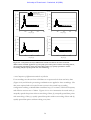
Figure 2-4 Sphere currents at various times (a – surface currents; b-d – equatorial/plane
currents) (after McNeill, 1980). ................................................................................................12
Figure 2-5 A permeable conducting sphere embedded in a conducting infinite space.
The dipolar source is located at S(r0,0,0) outside the sphere (after Singh 1973). ............14
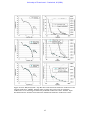
Figure 2-6 Time characteristic of hv1rr(t) for r/a=2, µ2/µ1=1, and variable σ1/σ2 (after
Singh 1973)...................................................................................................................................14
Figure 2-7 Time characteristic of hv1θr(t) for r/a=2, µ2/µ1=1, and variable σ1/σ2 (after
Singh 1973)...................................................................................................................................15
Figure 2-8 Time characteristic of hu1θθ(t) for r/a=2, µ2/µ1=1, and variable σ1/σ2 (after
Singh 1973)...................................................................................................................................15
Figure 2-9 “Reflected” smoke-rings. Electric field intensity is presented as sections for
20 consecutive time channels. The cyan and black contour lines present the
electric field intensity for a homogeneous 50 Ohm.m half space and indicate the
well-known diffusive smoke-ring behaviour. The colour contours indicate
electric field intensity of currents for a 5 Ohm.m prism (black rectangle) in a 50
Ohm.m half space as percentage of the half space response. The “reflected”
currents are clearly visible in channels 13 to 20. ...................................................................16
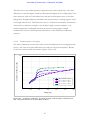
Figure 3-1 Comparison of apparent conductivity (calculated by differentiating the fitted
slowness with respect to reference depth curve) with the actual conductivity for
four three-layer models (after Macnae and Lamontagne, 1987). .......................................25
Figure 3-2
Cross-section of the model (top); Conductivity-depth image obtained by
differential S-transformation (centre); Conductivity-depth image obtained by
regularized S-inversion (bottom). (After Tartaras et. al., 2000)..........................................26
Figure 4-1 In (a) the raw data are presented in a contoured log-scale. In (b) the data
were normalised using the half space value used in the forward model. In (c) the
data were normalised as discussed above...............................................................................30
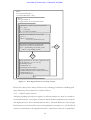
Figure 4-2 Flow diagram for decay curve slope analysis. ...............................................................32
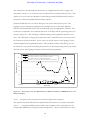
Figure 4-3 Percentage errors for differentiation in different domains of TDEM data for
a 10 Ohm.m half space. .............................................................................................................38
Figure 4-4 A Lagrange interpolating polynomial fitted to the data points outlining the
back of a duck (top) and a cubic spline curve fitted to the same data points
(bottom). (From Burden and Faires, 1993, Figures 3.11 and 3.12) ...................................40
Figure 4-5: Comparison of differentiation methods applied to (a) unequally spaced
points without smoothing of data, (b) unequally spaced points with smoothing of
iii
University of Pretoria etd – Combrinck, M (2006)
data, (c) equally spaced points without smoothing of data and (d) equally spaced
points with smoothing. ..............................................................................................................46
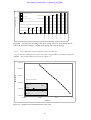
Figure 4-6: A summary (in ascending order) of the average error over twenty data points
for each of the alternatives in Figure 4.5. (ES: equal spacing, US: unequal spacing) .....47
Figure 4-7: Synthetic data and model for three-layer earth.............................................................47
Figure 4-8: Effects of smoothing at different points in S-layer transform algorithm................49
Figure 4-9: Comparison of S-layer differential transform results for the three numerical
differentiation methods applied on (a) unequally spaced data points without
smoothing of data, (b) unequally spaced data points with smoothing of data, (c)
equally spaced data without smoothing and (d) equally spaced data with
smoothing.....................................................................................................................................50
Figure 4-10: Four field data soundings; 1 to 4 are very smooth and considered to be
clean data, while 5 & 6 contains noise. ...................................................................................51
Figure 4-11: S-layer differential transform results for Sounding 1. ...............................................51
Figure 4-12: S-layer differential transform results for Sounding 2. ...............................................52
Figure 4-13: S-layer differential transform results for Sounding 3. ...............................................53
Figure 4-14: S-layer differential transform results for Sounding 4. ...............................................54
Figure 4-15: Half space resistivities compared to resistivities from S-Layer differential
transform. .....................................................................................................................................56
Figure 4-16:
Values for S and d corrections giving correct resistivity values and the
effective depth correction resulting from each pair. (from Excel: summary of
depth conversion factor models) .............................................................................................58
Figure 4-17: Cumulative conductance curves for late time halfsapce approximations. ...........60
Figure 4-18: Cumulative conductance curves for late time half space and S-layer
approximations............................................................................................................................61
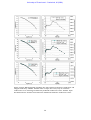
Figure 4-19:
Comparison of S-layer differential transform (SLDT) solutions using
different depth factors and layered earth inversions of synthetic data for a two
layer earth. ....................................................................................................................................63
Figure 4-20:
Comparison of S-layer differential transform (SLDT) solutions using
different depth factors and layered earth inversions of synthetic data for a three
layer earth (thin conductive layer)............................................................................................64
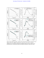
Figure 4-21:
Comparison of S-layer differential transform (SLDT) solutions using
different depth factors and layered earth inversions of synthetic data for a three
layer earth (thick conductive layer). Top: negative values included; Bottom: no
negative values. ............................................................................................................................65
Figure 4-22:
Comparison of S-layer differential transform (SLDT) solutions using
different depth factors and layered earth inversions of synthetic data for a thin
conductive plate in a resistive half space. ...............................................................................66
Figure 4-23:
Comparison of S-layer differential transform (SLDT) solutions using
different depth factors and layered earth inversions of synthetic data for a
conductive prism in a resistive half space...............................................................................67
Figure 4-24 Cumulative conductance versus depth, 0.02 S/m (50 Ω.m) half space...................69
Figure 4-25 Conductivity versus depth, 0.02 S/m (50 Ω.m) half space......................................69
Figure 4-26:
Cumulative conductance versus depth for two layers of decreasing
conductivity; first layer thickness 200m..................................................................................70
iv
University of Pretoria etd – Combrinck, M (2006)
Figure 4-27:
Imaged conductivity versus depth for two layers of decreasing
conductivity; first layer thickness 200m..................................................................................71
Figure 4-28:
Cumulative conductance versus depth for two layers of increasing
conductivity; first layer thickness 200m..................................................................................72
Figure 4-29: Imaged conductivity versus depth for two layers of increasing conductivity;
first layer thickness 200m. .........................................................................................................73
Figure 4-30: Imaged conductivity versus depth for two layers of increasing conductivity;
first layer thickness 200m – linear scale. .................................................................................73
Figure 4-31: Cumulative conductance for a 15m thick layer of varying conductivity at
150m depth in a 0.02 S/m half space......................................................................................74
Figure 4-32:
Imaged conductivity versus depth for a 15m thick layer of varying
conductivity at 150m depth in a 0.02 S/m half space..........................................................75
Figure 4-33:
Imaged conductivity versus depth for a 15m thick layer of varying
conductivity at 150m depth in a 0.02 S/m half space; linear scale. ...................................75
Figure 4-34: Cumulative conductance for a 0.2 S/m layer of varying thickness at 150m
depth in a 0.02 S/m half space.................................................................................................76
Figure 4-35:
Imaged conductivity for a 0.2 S/m layer of varying thickness at 150m
depth in a 0.02 S/m half space.................................................................................................77
Figure 4-36: Imaged conductivity for a 0.2 S/m layer of varying thickness at 150m depth
in a 0.02 S/m half space; linear scale.......................................................................................77
Figure 4-37: Cumulative conductance for a 2 S/m layer of varying thickness at 150m
depth in a 0.02 S/m half space.................................................................................................78
Figure 4-38: Imaged conductivity for a 2 S/m layer of varying thickness at 150m depth
in a 0.02 S/m half space.............................................................................................................78
Figure 4-39: Imaged conductivity for a 2 S/m layer of varying thickness at 150m depth
in a 0.02 S/m half space – linear scale. ...................................................................................79
Figure 4-40: Cumulative conductance for a 0.2 S/m layer of 20 m thickness at various
depths in a 0.02 S/m half space. ..............................................................................................80
Figure 4-41:
Imaged conductivity for a 0.2 S/m layer of 20 m thickness at various
depths in a 0.02 S/m half space. ..............................................................................................80
Figure 4-42:
Imaged conductivity for a 0.2 S/m layer of 20 m thickness at various
depths in a 0.02 S/m half space – linear scale. ......................................................................81
Figure 4-43: Cumulative conductance for a 0.2 S/m layer of 20 m thickness at 150 m
depth in various host rock conductivities...............................................................................82
Figure 4-44: Imaged conductivity for a 0.2 S/m layer of 20 m thickness at 150 m depth
in various host rock conductivities. .........................................................................................82
Figure 4-45: Imaged conductivity for a 0.2 S/m layer of 20 m thickness at 150 m depth
in various host rock conductivities - linear scale...................................................................83
Figure 4-46: Cumulative conductance for a 0.2 S/m plate of 20 m thickness at 150 m
depth in 0.02 S/m host rock. The horizontal dimensions vary from 100 m to
infinite. ..........................................................................................................................................84
Figure 4-47: Imaged conductivity for a 0.2 S/m plate of 20 m thickness at 150 m depth
in 0.02 S/m host rock. The horizontal dimensions vary from 100 m to infinite. .........84
Figure 4-48: Imaged conductivity for a 0.2 S/m plate of 20 m thickness at 150 m depth
in 0.02 S/m host rock. The horizontal dimensions vary from 100 m to infinite;
linear scale.....................................................................................................................................85
v
University of Pretoria etd – Combrinck, M (2006)
Figure 4-49: Cumulative conductance for a 2 S/m plate of 20 m thickness at 150 m
depth in 0.02 S/m host rock. The horizontal dimensions vary from 100 m to
infinite. ..........................................................................................................................................85
Figure 4-50: Imaged conductivity for a 2 S/m plate of 20 m thickness at 150 m depth in
0.02 S/m host rock. The horizontal dimensions vary from 100 m to infinite...............86
Figure 4-51: Imaged conductivity for a 2 S/m plate of 20 m thickness at 150 m depth in
0.02 S/m host rock. The horizontal dimensions vary from 100 m to infinite;
linear scale.....................................................................................................................................86
Figure 4-52: Cumulative conductance for a 0.2 S/m prism at 150 m depth in a 0.02
S/m host rock. The prism dimensions vary from 100 m to 400 m. ................................87
Figure 4-53: Imaged conductivity for a 0.2 S/m prism at 150 m depth in a 0.02 S/m
host rock. The prism dimensions vary from 100 m to 400 m. .........................................88
Figure 4-54: Imaged conductivity for a 0.2 S/m prism at 150 m depth in a 0.02 S/m
host rock. The prism dimensions vary from 100 m to 400 m; linear scale.....................88
Figure 4-55:
Comparison between imaged conductivities of a 0.2 S/m prism, 20 m
thick plate and infinite sheet of 20 m thickness at 150 m depth in a 0.02 S/m host
rock. Both the plate and prism have horizontal dimensions of 300 m.............................89
Figure 4-56: Cumulative conductance for 2 S/m prisms at 150 m depth in a 0.02 S/m
host rock. The prism dimensions vary from 100 m to 400 m. .........................................90
Figure 4-57: Imaged conductivity for 2 S/m prisms at 150 m depth in a 0.02 S/m host
rock. The prism dimensions vary from 100 m to 400 m. ..................................................90
Figure 4-58: Imaged conductivity for 2 S/m prisms at 150 m depth in a 0.02 S/m host
rock. The prism dimensions vary from 100 m to 400 m; linear scale..............................91
Figure 4-59 : Comparison between imaged conductivities of 2 S/m prisms, 20 m thick
plates and infinite sheet of 20 m thickness at 150 m depth in a 0.02 S/m host
rock. Plates and prisms with horizontal dimensions of 200 m and 300 m are
shown. ...........................................................................................................................................91
Figure 4-60: Examples of field data showing "returning smoke ring” behaviour (stations
-1200 and -150 from line 4950, Rosh Pinah data set)..........................................................92
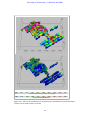
Figure 4-61: S-layer differential transform results (conductivity depth section) on
synthetic data. Top: Thin vertical plate (400mX 400m X 20m) .......................................94
Figure 4-62: Same models as in Figure 4-63. Red dots indicate half space decay
behaviour and blue dots indicate conductor in “free air” decay........................................95
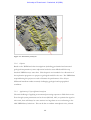
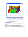
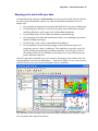
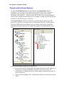
Figure 5-1: Mountain with TDEM survey team............................................................................... 101
Figure 5-2: Grid locality and layout. .................................................................................................. 102
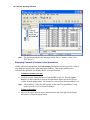
Figure 5-3: Line 4950, Station 100. Top: Raw data with calculated cumulative conductance
and imaged conductivity. Middle: No filter effect on input data values, only on
cumulative conductance curve with imaged conductivity of filtered conductance
values. Bottom: Input data filtered for late channel erratic behaviour and filtered
cumulative conductance values. ............................................................................................ 104
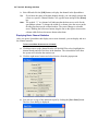
Figure 5-4: Line 4950, Station 300. Top: Raw data with calculated cumulative conductance
and imaged conductivity. Middle: No filter effect on input data values, only on
cumulative conductance curve with imaged conductivity of filtered conductance
values. Bottom: Input data filtered for late channel erratic behaviour and filtered
cumulative conductance values. ............................................................................................ 105
vi
University of Pretoria etd – Combrinck, M (2006)
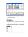
Figure 5-5: Line 4950, Station 400. Top: Raw data with calculated cumulative
conductance and imaged conductivity. Middle: No filter effect on input data
values, only on cumulative conductance curve with imaged conductivity of
filtered conductance values. Bottom: Input data filtered for late channel erratic
behaviour and filtered cumulative conductance values. ................................................... 106
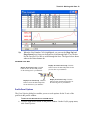
Figure 5-6: Line 4950, Station 450. Top: Raw data with calculated cumulative
conductance and imaged conductivity. Middle: No filter effect on input data
values, only on cumulative conductance curve with imaged conductivity of
filtered conductance values. Bottom: Input data filtered for late channel erratic
behaviour and filtered cumulative conductance values. ................................................... 107
Figure 5-7: Line 4950, Station -1550. Top: Raw data with calculated cumulative
conductance and imaged conductivity. Middle: No filter effect on input data
values, only on cumulative conductance curve with imaged conductivity of
filtered conductance values. Bottom: Input data filtered for late channel erratic
behaviour and filtered cumulative conductance values. ................................................... 108
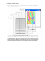
Figure 5-8: Comparison of SDTC filter only (top) and SDTC with additional noise filter
(bottom). Black dots are station elevations (DTM) and white dots represent
depths at which conductivities are calculated..................................................................... 110
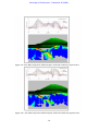
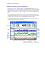
Figure 5-9: Line 450N showing good correlation between conductivity depth sections
obtained from the high (top) and medium frequencies (bottom). ................................. 111
Figure 5-10: Line 1650N showing poor correlation between the high (top) and medium
frequencies (bottom). .............................................................................................................. 112
Figure 5-11: Line 450; Stations750 and 1450; medium and high frequency measured data... 113
Figure 5-12: Line 1650; Stations -200, 150 and 250; medium and high frequency
measured data. .......................................................................................................................... 114
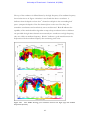
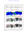
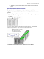
Figure 5-13: Contour map of conductor decay constants draped over topography and
conductivity depth sections in 3D. Top viewpoint is from inclination 20˚,
declination 180˚ and 5km distance. Bottom viewpoint is inclination 10˚,
declination -100˚ and distance 5km. Axes are Northing, Easting and Elevation
above sea level. ......................................................................................................................... 115
Figure 5-14: .3D view from inclination 60˚, declination 180˚ and 5km distance with and
without contour map of conductor decay constants. ....................................................... 116
Figure 5-15: Line 4050. EM response profiles and sections from automated processing
procedures. ................................................................................................................................ 118
Figure 5-16: Line 4150. EM response profiles and sections from automated processing
procedures. ................................................................................................................................ 119
Figure 5-17: Line 4050. Comparison of Maxwell plate model and conductivity depth
section. ....................................................................................................................................... 120
Figure 5-18: Line 4150. Comparison of Maxwell plate model and conductivity depth
section. ....................................................................................................................................... 120
Figure 5-19: EM Response over conductor................................................................................... 122
Figure 5-20: Conductivity depth section from S-layer transform, showing dipping
conductor................................................................................................................................... 123
Figure 5-21: Conductivity depth section in greyscale with channels corresponding to half
space power law decay indicated in red. .............................................................................. 123
vii
University of Pretoria etd – Combrinck, M (2006)
Figure 5-22: Conductivity depth section in greyscale with conductor decay constants
plotted at scaled channel positions. ...................................................................................... 124
Figure 5-23: Conductivity depth section in greyscale with channels on stations showing
sign changes indicated in blue................................................................................................ 124
viii
University of Pretoria etd – Combrinck, M (2006)
ACKNOWLEDGMENTS
The author wishes to thank Prof. Willem Botha (my supervisor) for his patience and
when it was required, the lack thereof. Many other people including family, friends,
training partners and colleagues contributed to this work through their continued moral
support. To Melinda de Swardt who took me for tea when the end seemed too far away
a special word of gratitude, as well as to all my students who stimulated my own growth
with their questions and enthusiasm.
Sincere gratitude is also extended to BHP Billiton for allowing me to use their data and to
that very special breed of geophysicists specialising in EM who published and shared
their knowledge without whom there would have been nothing to build this work on.
Lastly, to the Creator who thought it well to hide the earth’s riches from us, but not
without endowing us with the capabilities to find it if looking with courage and
persistence.
ix
University of Pretoria etd – Combrinck, M (2006)
Chapter 1
1
INTRODUCTION
"I believe that we cannot live better than seeking to become still better than we are."
(Socrates)
1.1
General overview
The Time Domain Electromagnetic (TDEM) method, also referred to as Transient EM
(TEM), has been used in mineral exploration since the late 1950’s. The basic theory of
this method is defined in totality by four differential equations, known as Maxwell’s
equations. These equations describe the relationships between electric and magnetic
fields and sources, enabling the geophysicist to derive the electric field (E) in the earth
through measuring the magnetic field (B), or it’s time derivative (dB/dt) on, above or
below the surface. The electric field in the earth is a function of the electromagnetic
(EM) source and of the earth’s conductivity distribution. If the source is known, the
geophysicist should be able to derive the conductivity distribution of the subsurface (and
therefore be able to isolate and interpret zones with contrasting conductivities).
•
The success of this procedure is dependant on three factors:
•
Choosing a source (transmitter) of appropriate dimensions and magnetic moment
to induce currents in the subsurface volume of interest
•
Measuring the induced magnetic field and/or its derivative with the required
accuracy and resolution in time and space (receiver) to resolve the target
•
Accurately solving Maxwell’s equations
The first two factors are concerned with the design of the measuring instrument and data
acquisition parameters. Survey costs are the largest limiting influence on these factors
and increases in cost can only be justified by producing increasingly accurate geological
models leading to savings in other stages of exploration expenses, e.g. drilling.
Theoretically, within some engineering constraints, one can choose to measure or
“know” the whole field exactly. This is a scenario utilised very effectively through
1
University of Pretoria etd – Combrinck, M (2006)
forward modeling and is the reason why synthetic data is normally used as a first run to
test new interpretation algorithms.
The third factor proves to be the most difficult – accurately solving Maxwell’s equations.
These equations can only be solved analytically for a few very simple geometrical models
and only if assumptions regarding homogeneity, isotropy, frequency dependence, and
frequency and conductivity ranges are made. Kaufman and Keller (1983) makes use of
asymptotic equations based on even more assumptions and terms like “far away”, “late
time”, “early time” and “large loops” are found extensively in EM literature. Solutions
are calculated for these very special instances of system geometry and conductivity
models, but the results are applied and compared to real earth situations, not complying
with these assumptions. Following this reasoning it is understandable why geophysicists
sometimes experience frustration in terms of knowing that there is a conductive unit but
not being able to say exactly what or where, leading to simply drilling anomalies – also
known as “bump-hunting”.
Accepting that Maxwell’s equations cannot be solved analytically for a general situation,
the next option would be to solve them numerically making use of standard numerical
solutions for differential equations. The complexity of these equations, numerical
instabilities under certain conditions (e.g. high conductivity contrasts), and the very long
computer calculation times, imply that full three dimensional solutions (and especially
inversion) of realistic geological models are not yet reaching industry expectations as an
efficient interpretation tool.
The only option left at this stage is to develop time- and cost efficient algorithms to find
solutions based on some of these assumptions and apply these only to geological settings
and data satisfying those assumptions. An example of this is the mathematical assumption
of one dimensionality of the earth, which is met when horizontally layered geology is
investigated. This approach implies a number of different interpretational procedures
and algorithms to be developed. It is of course possible to apply one algorithm or
procedure to all data acquired over a range of different geological settings, but the
obtained results would only be reliable if the inherent assumptions of the algorithm are
met.
2
University of Pretoria etd – Combrinck, M (2006)
One of the most common assumptions is that the host rock containing the ore body of
interest is very resistive. This implies a significant decrease in computational effort, but
unfortunately is one of the assumptions not always met in true field conditions. The
non- compliance of this assumption is of great importance in the closely related field of
landmine detection where small pieces of metal are looked for, often in very conductive
and magnetite rich top soils (Butler, 2003).
1.2
Objective
The objective of this work is to find an efficient, preferably automated, algorithm or
interpretational procedure that can be applied in real time to scenarios of conductors
buried in a resistive and/or conductive host rock or half space. This will not provide the
ultimate answer, but can be considered another useful tool available to the geophysicist to
reduce some assumptions. Real-time conductor location and imaging (i.e. estimating size,
depth and conductance) can attribute significantly to reduction of processing and
interpretaion cost in the mineral industry and might also encourage the development of
new instruments. For example, a multi-channel metal detector with real-time processing
and conductivity imaging of data might prove to be very valuable in the field of landmine
detection , especially in conductive top soil regions where traditional metal detectors
sometimes prove to be inadequate (Butler, 2003).
3
University of Pretoria etd – Combrinck, M (2006)
Chapter 2
2
OVERVIEW OF ELECTROMAGNETIC THEORY FOR GROUND, INLOOP TDEM DATA
"There is a theory which states that if ever anybody discovers exactly what the Universe is for and why it is here,
it will instantly disappear and be replaced by something even more bizarre and inexplicable. There is another
theory which states that this has already happened.”
(from “The Hitchhiker’s guide to the Galaxy”, Douglas Adams)
2.1
Introduction
It is the inherent complexity contained in the electromagnetic method that on the one hand
forces us to simplify it almost beyond recognition in order to apply it practically; and on
the other hand compels us to keep on searching for the “truth” (or the most complete set
of information that can be obtained from EM measurements). This continued search is
conducted in many, painstakingly slow, very small steps – sometimes referred to as
research.
All EM methods (except the magneto-telluric method) utilise active sources, or
transmitters, in order to generate measurable fields. This is in contrast to passive methods
such as the potential field methods (e.g. the gravity and magnetic techniques) where the
earth’s natural occurring magnetic field is measured. Passive source method instruments
only consist of receivers and the data acquired by different instruments are all reduced to
the earth’s total field with no or minimal computational effort. Active source instruments,
on the other hand, require the complete specifications of the source and receiver to be
incorporated into the processing and interpretational procedures. Unless stated otherwise,
algorithms derived in this study are only suitable for systems conforming to the same basic
geometrical set-up and operating parameters as described in the following paragraphs.
2.2
System geometry and operating specifications
The theory developed in this study is directly applicable to central-loop ground TDEM
systems with step-current excitation, e.g. Geonics EM37 or EM47 and interpretation
4
University of Pretoria etd – Combrinck, M (2006)
strategy allows for both 1D and 3D model considerations. The late time mathematical
approximations are implemented for most procedures.
2.3
Analytical TDEM responses for four common models
Analytical responses for TDEM data are calculated by solving Maxwell’s equations. The
differential forms of the equations are valid at points in space only, but comparatively easy
to calculate, while the integral forms are valid at boundaries of units, more difficult to
calculate and used primarily to generate boundary conditions.
Table 2-1 Maxwell’s equations (Compiled from Ward and Hohmann (1988) and Kaufman and
Keller (1983)).
Maxwell’s equations in integral form:
Maxwell’s equations in differential form:
∫ D ⋅ dS =q
∇⋅D = ρ
S
∫ B ⋅ dS = 0
∇⋅B = 0
S
∫ E ⋅ dl = −
dΦ B
dt
∇×E = −
∫
Φ B = B ⋅ dS = Flux through surface
S
∂D
∫ H ⋅ dl = I + ∫ ∂t
∂B
∂t
⋅ dS
S
∇×H = j+
∂D
∂t
Maxwell’s equations are uncoupled differential equations that need to be coupled using the
constitutive equations that contain all the electrical and magnetic properties of the medium
through which EM propagation occurs (i.e. the earth in geophysics). The constitutive
equations are given by Ward and Hohmann (1988) as:
D = ε⋅E
B = µ⋅H
j = σ ⋅ E.
E : electric field intensity [V/m]
B : magnetic induction [Tesla]
2
D : dielectric displaceme nt [C/m ]
I : current [A]
H : magnetic field intensity [A/m]
j : current density [A/m 2 ]
ρ : electric charge density [C/m3 ]
σ , σ : conductivi ty [S/m]
q : charge [Coulomb]
µ , µ : magnetic permeabili ty [H/m]
ε , ε : dielectric permittivi ty [F/m]
5
University of Pretoria etd – Combrinck, M (2006)
In these equations the dielectric permittivity, magnetic permeability and electric
conductivity should all be regarded as tensor functions of angular frequency, position, time,
temperature, pressure and magnetic/electric field strength. However, in order to derive
analytical solutions some assumptions regarding these parameters are necessary.
ASSUMPTIONS:
•
All media are linear, isotropic and homogeneous and possess physical properties,
which are independent of time, temperature and pressure (implying scalar
presentation of physical properties rather than tensors).
•
The magnetic permeability of all media is assumed to be equal to that of free space,
i.e. µ=µ0.
The TDEM solutions are derived by calculating the frequency domain electromagnetic
(FDEM) responses for equivalent models and then applying Fourier transforms to these
results. In order to solve the FDEM equations analytically some further assumptions are
necessary.
ADDITIONAL ASSUMPTIONS:
•
There are no free electric charges or current in the medium, i.e.
ρ = 0;
•
∇ ⋅ D = ∇ ⋅ E = 0.
We assume a harmonic time varying field, i.e.
E = E 0 e − iϖt and B = B 0 e −iϖt .
•
Displacement currents are much smaller than induction currents, i.e.
∂D
<< j and ∇ × H = σE implying a wavenumber of
∂t
k 2 = iωµσ in the solution of the wave (Helmholz) equation.
The receiver and transmitter are in the same plane of observation (z=0), also indicating the
air-surface boundary in the case of a half space or layered earth.
Incorporating these assumptions into calculations the analytical solutions for a number of
different geological models can be found. For the purposes of this study there are four
cases deserving special attention, namely:
•
Conductive half space
6
University of Pretoria etd – Combrinck, M (2006)
•
Thin, conductive sheet (S-layer)
•
Finite conductor in a resistive host rock (half space)
•
Finite conductor in a conductive host rock (half space).
2.3.1
TDEM central-loop response over a conductive half space
The quasi-static approximation of EM-field propagation in a half space can be described as
a diffusion process (Nabighian, 1979). When doing a TDEM survey the current in the
transmitter loop is switched off very abruptly, causing a sudden change in the associated
magnetic field (large ∂B/∂t). Following from Maxwell’s third equation the electric field (E)
associated with this sudden change in magnetic field will cause a current to flow in the
conductive half space ( j = σE ). This current will mimic the primary transmitter loop
geometry but will only exist in that form for a fraction of a second as it is not confined to a
specific path or circuit and has no source (battery) to maintain current flow. The induced
current will therefore immediately start to dissipate, generating a new magnetic field that
changes with time and consequently induce new currents in the half space. This behaviour
was discussed extensively by Nabighian (1979), leading to the smoke-ring concept of EM
propagation in a homogeneous half space. In short, a number of EM induced currents
exist in the half space after the primary field is terminated and the maximum current
density retains a transmitter loop-like shape expanding with time. Contouring the electric
field at different points in time clearly show the maxima of the electric field (most
dominant currents) migrating outward and downward into the half space at an angle of
approximately 30°. Nabighian (1979) also introduced the mathematical alternative of a
single equivalent current filament that will produce, with a high degree of accuracy, the
same EM fields measured on the surface of the earth, as would the whole system of real
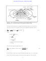
currents. This equivalent current filament moves outward and downward at an angle of
approximately 47°. A comparison of these two approaches is shown in figure 2.1. The
advantage of using the single equivalent current filament is the dramatic simplification in
mathematical description that allows the calculation of parameters such as velocity and
depth with time as well as relationships of these to half space conductivity.
7
University of Pretoria etd – Combrinck, M (2006)
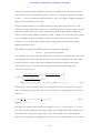
Figure 2-1 The use of equivalent current filament concept in understanding the behaviour of
TEM fields over a conducting half space (after Nabighian and Macnae, 1991).
The quasi-stationary (derivative of) magnetic field transient response of a central-loop,
step-current system over a conductive earth is given by Kaufman and Keller (1985) as
∂H z
I
=−
∂t
µ 0σa 3
(
)
2
⎡
−u 2 ⎤
2
⎢⎣3erf (u ) − π 12 u 3 + 2u e ⎥⎦
(2.1)
where
erf (u ) =
u=
2
π
u
−x
∫ e dx
2
0
π 2a
τ
⎛ 2t
τ = 2π ⎜⎜
⎝ µ 0σ
a = radius of
1
⎞
⎟⎟
⎠
the transmitter loop[m]
2
t = time [s],
with a late time asymptotic approximation of
Ia 2 (σµ 0 ) 2 − 5 2
∂H z
= (emf) ⋅ (effective receiver area) = −
t .
1
∂t
20π 2
3
In the “late time” (which can be achieved through either large values of t, or small values
of σ), it can be seen from equation 2.2 that the vertical component of the measured
8
(2.2)
University of Pretoria etd – Combrinck, M (2006)
electromotive force (emf) is directly proportional to t
−5
2
for an ideal step function
excitation. This behaviour is described as a power-law decay with time and manifests as a
straight line with a slope of m = –5/2 on a graph of log (emf) versus log (t). The horizontal
component of the emf can be shown to exhibit the same behaviour (Kaufman and Keller,
−3
1983); the only difference being that it shows a time-decay proportional to t in the late
time. In terms of the smoke-ring analogy, the “late time” for profiling commences when
the equivalent current filament is so far away that any receiver position can be
approximated to be at the centre of the smoke-ring. With the central-loop system (as used
in this study) this is always the case and it is easy to see why the late time approximations
are particularly useful for this survey geometry.
2.3.2
Thin, conductive sheet (S-layer)
Parameters used in the conductive sheet model are shown in figure 2.2.
Receiver loop
Transmitter loop
r
d
Thin, conductive sheet with conductance S Siemens.
Figure 2-2 Conductive sheet parameters.
The equivalent current smoke-ring behaviour for an S-layer (originally solved by Maxwell)
is described by Nabighian and Macnae (1991). With the primary field termination currents
are induced in the S-layer, once again representing the geometry of the transmitter loop.
As time passes the equivalent current filament retains it original size and intensity and only
appears to migrate downwards with a velocity related to the conductance of the S-layer as
v = 2 / Sµ 0 ms -1 (figure 2.3). This is an exact solution for velocity (v).
9
University of Pretoria etd – Combrinck, M (2006)
Transmitter loop
Thin, conductive sheet with
conductance S Siemens.
t=t1
t=t2
t=t3
Figure 2-3 Equivalent current filaments (images) for a conducting thin sheet at
various times after current interruption in the transmitter loop (after Nabighian
and Macnae, 1991).
The emf induced in a loop which is located in the horizontal plane, with a small dipole
source located at its centre, is given by Kaufman and Keller (1983) as:
emf = −
3(τ s + 2h0 )
M
2
Sr 1 + (τ + 2h )2
s
0
[
]
5
(2.3)
2
where
M = magnetic dipole moment of the transmitter (small) loop
τs =
2t
µ 0 Sr
r = radius of the large receiver loop[m]
t = time [s]
S = conductanc e of the thin plate [S]
d
r
d = vertical distance between the loops and the conductive plate.
h0 =
The quasi-stationary (derivative of) magnetic field transient response of a central-loop, step
current system over a thin conducive sheet can be calculated from equation 2.3 by applying
the principle of reciprocity (i.e. in any system the same emf will still be measured if the
transmitter and receiver geometries are interchanged). Making the late time approximation
10
University of Pretoria etd – Combrinck, M (2006)
of
2t
+ 2d >> r (where r now represents the small loop radius after reciprocity) and
µ0 S
simplifying equation 2.3 we have
3M
1
2
16 Sr (τ + d )4
emf late time
emf late time
∂H z
3M
1
=
=
=−
2
∂t
effective Rx area
16 Sπ (τ + d )4
nr πr
where
M = magnetic dipole moment of the transmitter (large) loop
emf late time = −
τ=
(2.4)
(2.5)
t
µ0 S
nr = number of turns in receiver loop
r = radius of the small receiver loop[m].
This is a very good approximation for the chosen system geometry as the radius of the
receiver loop is always in the order of one meter and the late time condition is always
satisfied under field conditions. The “late time” approximation of the S-layer response is
therefore directly proportional to t −4 . This behaviour manifests as a straight line with a
slope of m = –4 on a graph of log (emf) versus log (t).
2.3.3 Finite conductor in a resistive host rock (half space)
The significance of having a confined target surrounded by an insulator is that there is
always some stage of time (“late time”) when the current distribution in the conductor
becomes invariant with time and the decay becomes exponential at a rate determined by
the shape, size, and conductivity of the body (McNeill, 1980). An intuitive feeling for the
general behaviour of isolated (confined) conductors can be developed from examining the
simplified case of a conducting sphere assumed to be in a region of uniform magnetic field
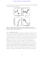
that is suddenly terminated. Immediately after termination of the primary current (early
time) the secondary currents flow on the surface of the sphere and are independent of its
conductivity (figure 2.4a). From then on the currents diffuse radially inwards, similar to the
smoke-ring propagation found in a half space. This stage of changing current distribution
is referred to as intermediate time (figure 2.4c). The late time commences when the
inductance and resistance associated with each current ring, have stabilized and from this
time onwards both the currents and their associated external magnetic field commence to
decay exponentially with a time-constant given by
11
University of Pretoria etd – Combrinck, M (2006)
τ=
σµa 2
π2
(2.6)
σ = conductivity of sphere [S]
a = radius of sphere [m],
so that
emf sphere late time = Ae
−t
τ
(2.7)
A = constant containing geometrical information.
Emf measurements taken at this stage of “late time” will manifest as a straight line when
plotted on a semi-log graph of ln(emf) versus time.
(b) Early time
(a) Early time
(d) Late time
(c) Intermediate time
Figure 2-4 Sphere currents at various times (a – surface currents; b-d – equatorial/plane
currents) (after McNeill, 1980).
2.3.4
Finite conductor in a conductive host rock (half space)
When a conductive target is located in a conductive host rock the inducing magnetic field,
at the location of the target, is no longer a step function but a slowly varying field due to
12
University of Pretoria etd – Combrinck, M (2006)
the diffusion of the smoke-ring currents (Nabighian and Macnae, 1991) and the
assumptions stated in 2.3 are not valid anymore. This different nature of the inducing field
has two consequences. Firstly, the toroidal vortex (induced) currents will not be as strong
as in the case of a conductor in free space, because of the reduced ∂B/∂t component
(fields are varying slower with time). Secondly, the smoke-rings will also cause galvanic
currents to flow in the conductor and lead to charge accumulation on the boundaries
between the conductor and the host rock. The smoke-ring electric field will
instantaneously be opposed within the target by the field of this electric charge distribution
created at the target boundaries. A secondary electric field created by these charges will
cause a poloidal current flow that tends to cancel most of the primary electric field (i.e. the
field associated with the smoke-rings) inside the conducting target (Nabighian and Macnae,
1991). This cancellation is more effective for short strike length bodies which, therefore,
have less poloidal (galvanic) current flow than longer bodies. The strength of these
currents depends mainly on the conductivity of the host rock and is only weakly dependent
on the much higher conductivity of the target. As such, the secondary magnetic field will
decay at a rate governed chiefly by the host rock conductivity. Anomalies due to both
poloidal (galvanic) and toroidal (inductive) currents are generally of the same sign and
increase the detectability of a given target according to Nabighian and Macnae (1991).
However, the combined anomaly will be spatially smeared toward longer wavelengths
compared to that of vortex currents alone – leading to erroneous interpretation if modelled
using a conductor in free-space approach. Singh (1973) has calculated the TDEM
response for a conductive sphere in a conducting infinite space and shown that the late
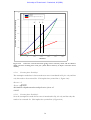
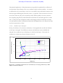
time response can also be presented as an inverse power law that is characteristic of wholeand half space responses (i.e. straight-line behaviour in the late time on a logarithmic graph
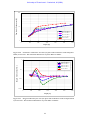
of emf versus time). In the following graphs, h refers to the magnetic field component, the
first subscript 1 to the multi-pole, the second to the spherical component (r, θ, or φ), and
the third to the orientation of the magnetic dipole (r for radial, θ for transverse). The
superscripts v and u refer to the magnetic mode or transverse electric (TE) and electric
mode or transverse magnetic (TM) solutions. In free space (i.e. making the quasi-static
approximation) only TE solutions are generated with a radial magnetic dipole as source
(horizontal loop above sphere). Figures 2.6 to 2.8 show the differences in late time decay
behaviour between a conductive sphere in free space (σ1/σ2=0) and a conductive sphere
in a conducting infinite space for various conductivity contrasts (σ1/σ2=1/10 to 1/100).
The secondary magnetic field component hv1rr(t) in figure 2.6, is equivalent to the vertical
13
University of Pretoria etd – Combrinck, M (2006)
component (hz(t)) generated from a vertical magnetic dipole source through abrupt
termination of current in a horizontal loop. The response for a sphere in free space
(σ1/σ2=0) corresponds with solutions obtained by Nabighian (1971) and McNeill (1980).
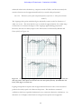
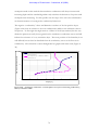
Figure 2-5 A permeable conducting sphere embedded in a conducting infinite space. The
dipolar source is located at S(r0,0,0) outside the sphere (after Singh 1973).
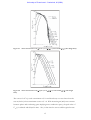
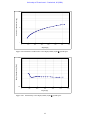
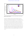
Figure 2-6 Time characteristic of hv1rr(t) for r/a=2, µ2/µ1=1, and variable σ1/σ2 (after Singh
1973).
14
University of Pretoria etd – Combrinck, M (2006)
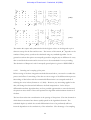
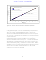
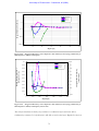
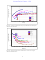
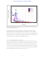
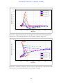
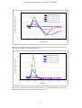
Figure 2-7 Time characteristic of hv1θr(t) for r/a=2, µ2/µ1=1, and variable σ1/σ2 (after Singh 1973).
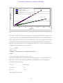
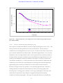
Figure 2-8 Time characteristic of hu1θθ(t) for r/a=2, µ2/µ1=1, and variable σ1/σ2 (after Singh
1973).
The curves for hv1rr(t) reach a maximum at T>0 and then decay at a rate slower than the
case σ1/σ2=0, whose maximum occurs at T =0. With increasing σ1/σ2 (lower contrast
between sphere and conducting space implying more conductive space), the peak value of
hv1rr(t) is reduced and delayed in time. Also, in late time the curves exhibit typical inverse
15
University of Pretoria etd – Combrinck, M (2006)
power law decays; straight lines with equal slopes, independent of the actual conductivity
values. Figure 2.7 shows the hv1θr(t) component as a function of time, once again
comparing free space with conducting space responses. The delayed and reduced peaks
with straight-line behaviour in the late time are still present, but the most interesting feature
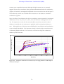
is the sign change that occurs in this response when a conducting space is introduced. The
last component of interest is the hu1θθ(t) in figure 2.8. This component doesn’t exist for
the free-space case and presents the magnetic field components associated with galvanic
currents generated in the sphere. These responses are comparable in magnitude to the
fields generated by the vortex currents. The sign changes observed in figure 2.7 can be
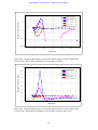
explained by thinking of the sphere acting as a secondary source of smoke-rings. Smokerings (or more probably shells) move out from this source in all directions and the moment
they pass the receiver position a sign change is recorded in the measured radial component
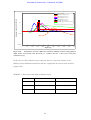
(figure 2.9).
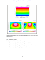
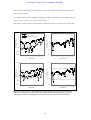
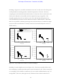
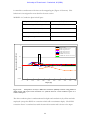
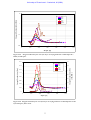
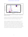
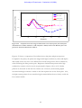
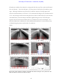
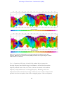
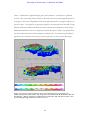
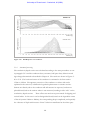
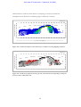
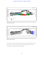
Figure 2-9 “Reflected” smoke-rings. Electric field intensity is presented as sections for 20
consecutive time channels. The cyan and black contour lines present the electric field intensity
for a homogeneous 50 Ohm.m half space and indicate the well-known diffusive smoke-ring
behaviour. The colour contours indicate electric field intensity of currents for a 5 Ohm.m prism
(black rectangle) in a 50 Ohm.m half space as percentage of the half space response. The
“reflected” currents are clearly visible in channels 13 to 20.
16
University of Pretoria etd – Combrinck, M (2006)
2.4
Conclusion
It is possible to describe electromagnetic field propagation analytically for only a few
simplified earth models. Modelling realistic geological environments imply numerical
solution of Maxwell’s equations which are very time-consuming and not yet commonly
used in industry. Several interpretation techniques and strategies have therefore been
developed based on the simplified equations given above and these will be discussed in the
following chapters.
17
University of Pretoria etd – Combrinck, M (2006)
Chapter 3
3
CONVENTIONAL INTERPRETATION TECHNIQUES
"The definition of insanity is doing the same thing over and over and expecting different results.”
(Benjamin Franklin, 1706-1790)
3.1
Introduction
The ultimate goal of doing any geophysical survey is to deliver a map or model indicating
the subsurface distribution of physical properties, i.e. conductivity in the case of TEM and
to interpret this data in terms of geology. When geological information are added to the
geophysical model it is possible to link lithology or structures to distinct geophysical units
of different conductivities and this serves as a very useful tool in constructing a final
geological model.
This study is concerned mainly with the conversion of TEM data to a reliable subsurface
conductivity distribution. Traditionally there are two separate classes of exploration targets
for TEM surveys and based on these classes different survey geometries and
interpretational procedures are followed. In modern day geophysics these two classes of
surveys increasingly overlap but it is still important to understand the different approaches
that were followed in the past as most of the interpretation techniques being used today
were developed for very specific target conditions.
The first type of target is considered to be a confined conductor(s) in a resistive host rock.
The theoretical assumptions made in this case are basically that the host rock has no
influence on the electromagnetic propagation of fields and conductors are considered to be
suspended in free space for all mathematical purposes. TEM surveys to detect this type of
target are designed to emphasize lateral variations in conductivity and are called profiling
surveys. The geophysical model derived from interpreting a survey like this would contain
the location, conductivity and geometrical parameters of one or more finite conductors
(two- or three-dimensional). These conductors would be simplified geometrical shapes
such as spheres, ellipsoids, plates or prisms approximating true geological units. Typical
geological targets are massive sulphides or linear structures like weathered faults or shear
zones.
18
University of Pretoria etd – Combrinck, M (2006)
The second type of target is considered to be a half space or layered earth. The theoretical
assumptions made in this case are that there are no finite conductors present and that the
subsurface layers are perfectly horizontal. Mathematically this means that all processing
reduces to one dimension. TEM surveys designed for this type of target emphasize vertical
variations in conductivity and are called sounding surveys. Fairly realistic models of the
subsurface are obtained by stitching together a number of sounding models to produce a
conductivity depth section and effectively resolving geological features in two dimensions
and not only one. Practical applications would include determining depth to bedrock or
mapping saltwater intrusions into aquifers.
In reality a combination of these two approaches are necessary to obtain a complete
subsurface conductivity distribution and it is towards this goal that most TEM research is
currently focused. The most important factor when dealing with the huge amounts of data
gathered in this instance is to automate as much of the processing and interpretation as
possible in order to keep survey time and costs competitive in the exploration industry. At
the same time it is important to resolve less conspicuous anomalies and map them more
accurately as the tradition of “bump-hunting” is not profitable in modern day exploration.
In the rest of this chapter the different techniques used in TEM interpretation will be
discussed with reference to the optimum targets for interpretation as well as the potential
for automation of these techniques.
3.2
Profiles versus soundings
Profiling and sounding can refer to different survey geometries or just to the way data is
viewed, processed and interpreted. The same data set (or parts of it) can therefore be
treated as either sounding- or profile data or both. The most relevant view or
interpretation strategy is dependent on the primary target or goal of the survey as described
in 3.1. Interpreting data in profile format involves looking at measured values as a function
of distance, removing a half space response if required, and interpreting anomaly shapes
associated with two- or three-dimensional conductors either through forward modelling,
inversion or curve matching. This is very similar to modelling potential field data, but with
some important differences.
There are as many profiles to consider as there were time channels measured (varying
anywhere from 7 to 100) and often it is not possible to obtain a good fit for a specific
conductor on all of these channels simultaneously. This can be ascribed to the fact that
19
University of Pretoria etd – Combrinck, M (2006)
modelling software still approximates complex geological units in terms of simplified
geometries as well as mathematical simplifications sometimes needed to solve a problem
(see 2.3). Since TEM is an active source method (as opposed to magnetics and gravity) the
transmitter current waveform, geometry and position all determine the actual shape and
amplitude of anomalies. Different systems also measure different components of the
magnetic field or its time derivative, again resulting in different anomaly shapes and
amplitudes. Even if all the above factors are accounted for, the TEM method allows only
for modelling of time varying current distributions unlike gravity, for example, where the
measured field is a direct and unique consequence of the subsurface density distribution.
Interpretation of data in sounding format implies that a model is constructed with variation
in depth only, and such a model always takes the form of a number of layer thicknesses
and corresponding conductivities. Data are presented either as emf(t), ∂B/∂t, B(t) or more
commonly, apparent resistivity as a function of time. As with profiling data, a model is
determined through forward modelling, inversion or curve matching. Due to the onedimensional nature of this interpretation, inversion can be applied successfully provided
that the number of layers is known, a good starting model is used and the geology
conforms fairly closely to the one-dimensional assumption made in these algorithms.
3.3
Forward Modelling and Inversion
Forward modelling is a process whereby a geophysicist tries to match field data with
calculated values from a specified model by changing the model parameters until there is a
close correlation between the field and calculated data. Inversion is a mathematical
approach also described as optimization, minimization or solution of a system of nonlinear equations. Most of the various inversion approaches (an exception is Occam’s
inversion) reduce to the guessing of an initial model (initial parameters), forward calculating
the response of this model, determining the difference (error) between the calculated and
measured response and adjusting the initial parameters in a way that would minimize this
difference. A number of forward modelling and inversion algorithms have been published
ranging from a single current filament approximation (Barnett, 1984) through to the most
general case of complete three-dimensional models (Newman et. al., 1986; Newman and
Hohmann, 1988; Xiong, 1992; Wang and Hohmann, 1993).
20
University of Pretoria etd – Combrinck, M (2006)
3.4
Limitations on automation of inversion techniques
Forward modelling as defined in 3.3 cannot be automated as it includes the active
involvement of a geophysicist at every guess of a new model. In fact, inversion is the
process whereby “guessing of models” is taken over by an algorithm or computer.
Although mathematically sound, in practice there are a number of problems which often
inhibits the successful implementation and automation of inversion procedures.
•
A priori knowledge of the geology under investigation is needed; i.e. should
inversion be run for a layered earth (with how many layers) or should it be done for
multiple plates (and how many plates)?
•
Even if the general structure is known, the initial model should be close to the real
model to obtain mathematical convergence.
•
In the case of convergence, it can be difficult to decide whether convergence was
to the desired global minimum or just a local minimum which adds yet another
unknown to the interpretation process.
•
Equivalence
•
Validity of assumptions; e.g. late time behaviour of models are compared with time
channels exhibiting early or intermediate time behaviour.
•
There have to be more data than free parameters which would become a problem
when trying to implement a totally general three-dimensional cube as model (this
would of course be the ultimate solution).
•
The most limiting factor however, is the need for a very fast forward modelling
algorithm. TEM algorithms are still very time-consuming for all but the simplest
cases of layered earths and multiple plates.
Practical experience in the interpretation of TEM data with inversion software has shown
that extensive forward modelling was needed before inversions could be run successfully
and that the 3-10% statistical reduction in error did not always mean that a more
geologically plausible model was achieved. In fact, correlation with geological data such as
borehole and structural information proved invaluable to distinguish between mathematical
equivalent models and more often than not mathematical accuracy had to be sacrificed to
obtain geological feasibility in a model. This is especially true in a geologically complex
area. The best of both worlds would naturally be the application of constrained inversion,
21
University of Pretoria etd – Combrinck, M (2006)
where mathematical solutions are found subject to geological truths such as dip, strike,
conductivity ranges and limits on dimensions of bodies. However, this information is very
rarely available in the exploration industry before TEM interpretations have to be done.
Consequently, it is very difficult at this point in time to see inversion as a fully automated
procedure for interpretation of TEM data, although it could possibly be involved as a final
stage of processing after initial models have been found through alternative routes.
3.5
Decay curve analysis
Decay curve analysis is an extremely useful tool with its major strength probably being
simplicity. The TEM method is based on current distribution changes with time, and
decay curve analysis is the simplest way of analysing the time-varying fields associated with
this phenomenon. In Chapter 2 the specific equations describing the decay behaviour for
general models were given with specific reference to the late time. A summary of these late
time approximations is given in Table 3.1. Decay curve analysis is a tool that helps the
interpreter to distinguish between the two basic classes and subsequent interpretation
strategies as mentioned in 3.1. Plotting all data, station by station, on both log-log and loglinear graphs and analysing the slopes of any data forming straight lines in the late time
yields very good information on the geological structure in two dimensions. It allows the
interpreter to immediately divide the survey area up into regions containing the four
models shown in Table 3.1, with the only complication that a conductor in conductive host
rock and with very low contrast may be grouped with half space occurrences at this point.
However, what is more likely to happen from experience in Case History 1, Chapter 5, is to
find stations showing both isolated conductor and half space behaviour but at different
time channels. Similar behaviour was also described at the Elura massive sulphide deposit
which is situated under a conductive overburden, Australia, by Spies (1980). Decay curve
analysis as described here doesn’t give any information on depth of conductors, although
the decay constant (τ) found from inverse slope of model 3 (and sometimes model 4)
graphs is related to the dimensions and conductivity of the causative conductor McNeill
(1980), allowing a further division to be made between targets worth further investigating
or not. In instances where the subsurface geo-electrical structure is too complex to be
approximated by either of the models in Table 3.1, neither of the described characteristics
will be found on the decay curve and stations like this will form a class of their own and
require some special attention in later stages of interpretation. One of these more complex
decay curves involves a sign change in the vertical component of the ∂B/∂t measurements
22
University of Pretoria etd – Combrinck, M (2006)
inside the transmitter loop. It is impossible to see this behaviour in a conductive half space
or layered earth environment and it therefore implies either an IP effect or extensive lateral
variations (including two- or three-dimensional conductors) in the subsurface.
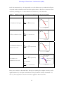
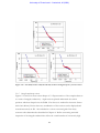
Table 3-1 Summary of late time approximations and behaviour for four general models.
Late time behaviour
1. Conductive half space
∂H z
5
∝ t − 2 (Power law)
∂t
Decay plot properties
Log (emf)
Model
m=-2.5
2. Thin, conductive layer
∂H z
∝ t − 4 (Power law)
∂t
Log (emf)
Log (time)
m= -4
3. Confined conductor in
resistive host rock.
−t
∂H z
∝ e τ (Exponenti al)
∂t
Log (emf)
Log (time)
m=-1/τ
High contrast:
4. Conductor in
∂H z
∝e
∂t
conductive host rock.
Low contrast:
−t
τ
(Exponenti al)
∂H z
∝ t −v (Power law)
∂t
Log (emf)
time
Low contrast:
m=-v (2.5)
High contrast:
-t/τ
emf ∝ e
Log (time)
Decay curve analysis as described here, although not yielding the complete solution, can be
applied without any user input and therefore has the potential to be fully automated. It is
also very fast compared to inversion and can be applied to data in real time.
23
University of Pretoria etd – Combrinck, M (2006)
3.6
Transforms (Depth imaging)
Spies and Frischknecht (1991) describe depth imaging techniques as low cost (i.e. fast and
automated) alternatives to modelling and inversion to provide an approximate image of the
resistivity section directly from observed data. Originally developed as a “processing” step
they now appear very useful for interpretation. Today there are a number of different
imaging schemes or transforms (Macnae and Lamontagne, 1987; Nekut, 1987; James, 1988;
Eaton and Hohmann, 1989; Smith et. al., 1994; Wolfgram et al., 1998; Tartaras et al., 2000),
all based on simplifying some of the governing equations to such an extent that a direct
solution for the depth and conductivity parameters can be found either analytically or
through curve matching. Although not as accurate as full modelling or inversion the
advantages of these schemes are computational speed and no need for initial models or
other interactive user input. These methods can therefore be considered as completely
automated.
3.6.1
Conductivity Depth Images (CDI’s)
This technique has been developed by Macnae and Lamontagne (1987) for step-response
sounding data and is routinely used in processing airborne TEM data. At each delay time
the variation of the step-response as a function of geometry is transformed to an equivalent
reference depth h, which can be related to the depth of electromagnetic field diffusion.
The behaviour of h as a function of delay time is nearly independent of the source-receiver
geometry. The slowness ∂t/∂h divided by the magnetic permeability is almost exactly
proportional to the cumulative conductance measured from the surface down to a depth h.
Thus an apparent conductivity (termed the “imaged conductivity”) can be estimated at
depth by ∂2t/µ0∂h2. The result is a conductivity-depth section that can be generated
automatically with no prior input needed from the operator. This method is based on the
receding image theory of a plane (or S-layer).
3.6.2
Stationary current images (SCI) (SCI - trademark of Geoterrex-Dighem Pty Limited)
This method highlights the edges of conductors, gives an indication of dip and allows a
qualitative estimate of the conductance of localized conductors (Wolfgram et al., 1998).
The SCI emphasizes structural features because it is optimised for lateral contrasts in
electrical conductivity. It is an empirically developed method only applied to GEOTEM®
24
University of Pretoria etd – Combrinck, M (2006)
system data and only results applied to synthetic data are available in literature (GEOTEM
(APPARENT) CONDUCTIVITY
is a registered trademark of Geoterrex).
102
102
101
101
100
100
10-1
10-1
10-2 0
10
101
102
DEPTH (h)
103
(APPARENT) CONDUCTIVITY
102
10-2
100
101
DEPTH (h)
102
102
101
100
101
10-1
100 0
10
101
DEPTH (h)
102
10-2 0
10
101
102
DEPTH (h)
103
Figure 3-1 Comparison of apparent conductivity (calculated by differentiating the fitted
slowness with respect to reference depth curve) with the actual conductivity for four three-layer
models (after Macnae and Lamontagne, 1987).
3.6.3
S-layer differential transform
The S-layer differential transform was originally developed by Sidorov and Tikshaev (1969)
and extended to an inversion technique by Tartaras et al., (2000). It is based on the latetime ∂Bz/∂t approximation of the S-layer model. The derivative of this equation (∂2Bz/∂t2)
is calculated and from these two equations the variables S (cumulative conductance) and d
(depth) can be solved for at every time channel. Taking the partial derivative of S to d
(∂S/∂d) gives the conductivity of a thin layer at depth d. The actual calculations are
remarkably simple and when working in a conductive, layered region this method gives
good results. The main criticism against the method (Tartaras et al., 2000) is the fact that it
contains two numerical differentiations which are numerically unstable operators and
therefore is extremely sensitive to noise. It is further based on the one-dimensional and
late-time assumptions. Although, for the central-loop sounding geometry it can be shown
(Tartaras et. al., 2000) that measured data almost always satisfy the late-time prerequisite.
25
University of Pretoria etd – Combrinck, M (2006)
Figure 3-2 Cross-section of the model (top); Conductivity-depth image obtained by differential
S-transformation (centre); Conductivity-depth image obtained by regularized S-inversion
(bottom). (After Tartaras et. al., 2000)
26
University of Pretoria etd – Combrinck, M (2006)
3.7
Combining Strategies
Interpreting geophysical data almost never comprises the straightforward application of a
fixed procedure. As with putting together the different pieces of a puzzle, the more
information you have and the more angles you can view it from, the better your chances
are of success. TEM data and processing are no different. Especially in TEM data there
are still so many approximations made in even the best processing and interpretation
algorithms that not one of them can be considered completely accurate. Automatically
implementing and combining decay curve analysis with an improved imaging algorithm to
isolate conductors will be discussed in the next chapter.
27
University of Pretoria etd – Combrinck, M (2006)
Chapter 4
4
AUTOMATED INTEGRATED ANALYSIS OF TDEM DATA
“Nature is not a competition. It doesn’t really matter, when you go out, if you don’t identify anything. What
matters is the feeling in the heart.” (Richard Adams, B. 1920, British Writer)
"Exploring the unknown defines the essence of humanity." (The author)
4.1
An integrated analysis algorithm
A software supported approach was developed for the:
•
More effective visualization of the field data for rapid anomaly detection
•
Automatic calculation and visualization of decay curve characteristics
•
The use of the S-layer transform for the creation of conductivity-thickness cross
section for the outline of finite conductors.
An automation of some strategies as outlined in chapter 3 was implemented in a C++
algorithm. Data analysis is performed on a time basis (i.e. decay curves) and not on a spatial
basis (i.e. profile plots). Furthermore, the S-layer transform part of the algorithm assumes
centre of the loop (sounding) data only. The algorithm does an automatic analysis,
discussed below, of each measured decay curve. The only user input required is to specify
system parameters and regression analysis limits, although default values for these are
given.
4.2
Visualization of the field data for rapid anomaly detection
Even though the ultimate gaol of TEM interpretation is to end up with a conductivitydepth section or conductor location and properties, it is always good to have the original
data readily available as well. This often helps to clarify ambiguities in interpretations or
models, e.g. the presence of a small, three-dimensional feature visible on raw data profiles
would imply possible failure of layered interpretations in that region. Noise is also
identified with more confidence on original data than after processing or transforms. TEM
data can, however, be quite challenging to present in a complete manner without losing
detail. Two factors contributing to this are the logarithmic span of data (with the small,
28
University of Pretoria etd – Combrinck, M (2006)
late time values often being more significant) and the fact that the half space (or
background) response often dominates that of the target.
A very simple approach was followed to minimize the effects of these two factors. Data at
every station are presented as a fraction of an average response calculated over the
complete data set. The reasoning behind this is that background (half space or layered
earth) should contribute the most to measured values over a large data set (as conductor
responses are considered “anomalous” to this background). Adding all these responses
together and calculating an average value at each time channel leads to the average
response expected in a specific survey area. The fraction responses (∂Bz/∂t divided by
average) at every station then show deviations of a station from the average or background
response. The advantage of this type of data presentation above standard profiles is that it
can be displayed as colour contoured pseudo-sections giving the same priority to all time
channels and very successfully enhancing anomalous regions. An example of this
procedure on synthetic data is shown in figure 4.1. The success of this procedure is of
course dependent on a relatively similar background response over a given survey area,
although fairly good results have been obtained in the case history discussed in chapter 5,
which was conducted over a complex geological area. The same presentation of data
(although independently developed) was also found in a paper by Eaton and Hohmann
(1987). In their case, however, the conductor to half space response was considered as a
signal to noise ratio and was examined for different survey geometries.
29
University of Pretoria etd – Combrinck, M (2006)
Figure 4-1 In (a) the raw data are presented in a contoured log-scale. In (b) the data were
normalised using the half space value used in the forward model. In (c) the data were normalised
as discussed above.
4.3
Decay curve analysis
The decay curve analysis is implemented in three steps.
•
Decay curves analyzed for layered earth (i.e. power law) behaviour.
•
Decay curves analyzed for exponential decay indicating confined conductors.
•
Decay curves analyzed for sign changes not related to noise.
30
University of Pretoria etd – Combrinck, M (2006)
4.3.1
Layered earth behaviour
The objectives of this analysis are:
•
to determine whether there is any straight line behaviour in the logarithmic domain
of a sounding data set;
•
to determine the largest number of channels (and channel numbers) on which the
behaviour can be found;
•
to test whether these slopes are close to either -2.5 or -4 and consequently
•
to classify the sounding as half space or S-layer type.
Firstly, the time channels and corresponding absolute ∂Bz/∂t values are transformed to the
logarithmic domain. The next step is to determine which channels (if any) approximate
straight line behaviour the best. The “best fit” is based on the correlation coefficient (R2);
the closer it is to one, the closer the data display power law decay behaviour. All possible
combinations of channels are tested starting with the user-specified minimum number of
channels, the default being four. The least squares fit for channels one to four is therefore
calculated, followed by two to five, three to six, etc. Then the number of channels is
increased by one and the whole process repeated, i.e. channels one to five are analysed,
followed by two to six, etc. This process continues until the number of data points
evaluated is equal to the number of points in the data set and only one least squares fit is
done, e.g. channels one to twenty. For every combination of channels the results are tested
to determine the “best fit”. The “best fit” combination will have a R2 value that falls within
a specified range; it will have the slope closest to either -2.5 or -4; and if there are two
combinations having the same properties thus far priority is given to the value
corresponding to the largest number of channels and latest times (figure 4.2).
31
University of Pretoria etd – Combrinck, M (2006)
Repeat
for NumberOfChannels=4
to NumberOfChannels=(20-4)
Repeat
for beginChannel=0
to beginChannel=(20-NumberOfChannels)
Calculate least squares regression parameters:
m := slope
c := y-intercept
R := correlation coefficient
2
Calculate closest distance of m to either
-2.5 or -4
mError = minimum of
abs(m+2.5) AND abs(m+4.0)
Test whether calculated parameters fall
within user-specified (or default) limits.
if (R > SpecifiedRegressionLimit) AND
(mError < SpecifiedSlopeLimit)
2
NO
YES
Assign parameters to “best fit” combination and
set this distance to -2.5 or -4 as new
SpecifiedSlopeLimit.
combinationR =R
SpecifiedSlopeLimit=mError
combinationBeginChannel=beginChannel
combinationNrOfChannels=NumerOfChannels
combinationSlope=m
combinationIntercept=c
2
2
Figure 4-2 Flow diagram for decay curve slope analysis.
Based on the decay curve analysis function every sounding is classified as exhibiting half
space behaviour, S-layer behaviour or neither of these.
4.3.2
Confined conductor behaviour
Analysing soundings for behaviour typical of confined conductors is done very similar to
the layered earth case. Once again, all stations and all channel combinations are analysed
with higher priority to more channels and later times. The main difference is that straight
line behaviour is now looked for in the semi-logarithmic environment, i.e. only the ∂Bz/∂t
values are transformed to the logarithmic domain. Furthermore, there are no predefined
32
University of Pretoria etd – Combrinck, M (2006)
slope values that need to be tested for and any regression fit within the specified R2 limit is
accepted as a possible conductor. The channels exhibiting the exponential decay are stored
as well as the decay constant which is calculated as the inverse of the “best fit” slope.
4.3.3
IP effect or severe lateral variation in subsurface conductivity
The test for sign change of the ∂Bz/∂t component is done because with the central loop
sounding configuration it implies a deviation from a layered, quasi-static subsurface.
Sign
changes can be ascribed to an IP (induced polarization) effect or significant lateral
variations in the subsurface conductivity distribution, including two- or three-dimensional
geological units. Having negative values of ∂Bz/∂t in a data set does not necessarily imply a
sign change and it is important to distinguish between a well sampled, repeatable sign
change and (normally late time) erratic noise. This was done by requiring at least two
points of a specific sign to be followed by four points of opposite sign before a sign change
is flagged in the data.
4.3.4
Results, output and presentation
The process of decay curve analysis as described here is extremely quick and takes less than
a second for 1600 stations on a Pentium IV PC. The parameters determined through these
functions are written to the output ASCII file and can be presented in GEOSOFT as
symbols on plan or pseudo-section format. A very useful presentation for first anomaly
isolation was also found through contouring the calculated decay constants (see Chapter 5).
This immediately allowed areas of anomalous conductivities to be isolated in plan view. It
is important to remember that all these procedures will indicate positions of anomalous
data points and not yet positions of conductors themselves.
4.4
4.4.1
Numerical calculation of the S-layer differential transform
Defining the S-layer transform
The S-layer differential transform was discussed briefly in paragraph 3.4.3. It was chosen
as the preferred imaging algorithm to include in the Sounding Interpretation program for
the following reasons,
33
University of Pretoria etd – Combrinck, M (2006)
•
Speed
•
No need for an initial model
•
Although it is based on the same imaging principles as the CDI transform it is
easier to implement with fewer empirical factors that need to be included
•
The late time approximation used in the algorithm is very applicable to the impulse
response, central-loop configuration this work is based on
•
For the specific case of a conductive host rock environment the S-layer differential
transform shows good resolving capabilities
•
As mentioned by Tartaras et. al. (2000) the main drawback of this method is the
fact that it requires a numerical differentiation scheme which tends to introduce
noise in the interpretation results. The implementation of a robust, yet accurate
numerical differentiation scheme based on the specific properties of TEM data
therefore receives high precedence. Further enhancements include a noise filter
based on data points satisfying the theoretical conditions for the S-layer transform.
The S-layer differential transformation results in two equations that have to be solved for
every time channel obtained at every station. Originally derived by Sidorov and Tikshaev
(1969) these are summarised by Tartaras et. al. (2000) as:
⎛ 5 ⎞
⎜⎜ V 3 ⎟⎟
16π 3
⎝
⎠
S=
4
⎛ 4 ⎞
(3M ∑ n ) 13 µ 0 3 ⎜ V ′ 3 ⎟
⎜
⎟
⎝
⎠
⎞
⎛
1 ⎜ 4V
⎟
−
− t⎟
d=
⎜
′
µ S⎜ V
⎟
0 ⎝
⎠
1
( 4.1)
( 4.2)
34
University of Pretoria etd – Combrinck, M (2006)
where
S = cumulative conductance [S]
d = depth [m]
M = magnetic dipole moment of transmitter [Am 2 ]
2
∑ = receiver area [m ]
n = number of turns of receiver coil
t = time [s]
⎛ ∂B
⎞
V = electromotive force of ideal receiver loop [V] = − ∑ n⎜⎜ z ⎟⎟
∂t
⎝
⎠
′
V = time derivative of measured voltage V [V/s].
The time derivative of the measured voltage (|V|’) is the parameter that has to be
determined through numerical differentiation. This value is used to calculate both
cumulative conductance (S) and depth (d) of an equivalent S-layer for each time channel
and noise generated by differentiation will consequently be introduced into both these
numbers. However, in order to find the earth parameter of interest, conductivity (σ),
another numerical differentiation has to be performed as,
σ (d ) =
∂S
[Siemens.m - 1]
∂d
(4.3)
which follows from the definition of cumulative conductance. Thus, not only is a new set
of errors generated in this step, but all errors from the first differentiation are carried over
and enlarged by this second differentiation.
The following features are investigated:
•
three numerical differentiation techniques are analysed in terms of the
specific nature of TDEM data, as described above
•
the most appropriate use of smoothing filters
•
the effects of the re-sampling of data points to equal time intervals.
35
University of Pretoria etd – Combrinck, M (2006)
4.4.2
Numerical differentiation of TEM data
In the late time, TDEM responses measured over a one-dimensional subsurface can be
described as a power-law function, equation 4.4, with k=2.5 for a half space and k=4 for a
thin conductive layer (S-layer). This creates the possibilities of using standard polynomial
approximations, but in the logarithmic and semi logarithmic domains. Consider the
following power-law decay:
V (t ) = At − k
A = constant
( 4 .4 )
k = decay constant
If the natural logarithm of this function is taken on both sides, it becomes,
ln(V (t )) = ln A − k ln(t )
( 4.5)
Substituting ln(V(t)) with y(x), ln(t) with x and –k with m, we end up with the equation of a
straight line (and a polynomial function) in the logarithmic domain.
If there is a two- or three-dimensional conductor present it will contribute to the latetime response in the form of an exponential function as shown in equation 4.6.
V (t ) = Ae − kt
(4.6)
A = constant
k = decay constant
If the natural logarithm of this function is taken on both sides, it becomes,
ln(V (t )) = ln( Ae − kt ) ⎫⎪
⎬
ln(V (t )) = ln A − kt ⎪⎭
( 4. 7 )
Equation 4.7 is again a linear function in the semi-logarithmic domain. This behaviour
only becomes dominant on TDEM sounding data if the conductor is much more
conductive than the surrounding host rock or when the host rock response has been
removed from the data through subtraction or deconvolution. Raw field data (as on which
the S-layer differential transform is normally applied) would mostly exhibit predominantly
power-law decay, although it will be distorted slightly in the presence of conductive layers
or finite conductors. In the logarithmic domain TDEM data appear as functions deviating
from a general linear trend and can be locally approximated by second or third order
polynomials. Finding a relationship between the derivative of a function and the derivative
of the same function in the logarithmic or semi-logarithmic domains would enable us to
36
University of Pretoria etd – Combrinck, M (2006)
apply polynomial-based differentiation techniques to data in the domain where they can be
approximated best by polynomial functions. These very specific properties of being
logarithmically sampled and exhibiting power-law or exponential decays make TEM data
distinctly unsuitable for the most common numerical differentiation schemes such as the
Lagrange formulas (Burden and Faires, 1993) which are based on functions exhibiting
polynomial behaviour.
4.4.2.1
Analytical relationship between derivative transforms in the various domains
The objective is to find an analytical relationship between the derivative of a function in the
linear domain (V’(t)) and the derivatives calculated in the semi-logarithmic (g’(t)) and
logarithmic domains (h’(ln(t))) respectively. The strategy is simply to apply the chain rule
of differentiation to functions presenting the data in the different domains.
Semi-logarithmic domain
In the semi-logarithmic domain the natural logarithms of the V values are taken and treated
as a function of (linear) time. It is presented by the function g(t)=ln(V(t)).
g (t ) = ln V (t )
∴V ' (t ) = V (t ) ⋅ g ' (t )
(4.8)
Logarithmic domain
In the logarithmic domain the natural logarithms of both the V values and times are taken
and the function h(ln(t))=g(t)=ln(V(t)) is plotted against ln(t). A substitution of variables
is made to simplify the derivation.
h[ln(t )] = ln[V (t )]
[ ( )]
h[ln(t )] = ln V eln (t )
Now, let x = ln(t ) and t = e x .
Then
[ ( )]
h' (x ) = D {ln[V (e )]}
1
.V ' (e ) ⋅ e
h' ( x ) =
V (e )
h(x ) = ln V e x
x
x
x
x
x
( )
h' ( x ) ⋅ V e x ⋅
1
ex
( )
= V ' ex
∴V ' (t ) = h' (ln(t )) ⋅ V (t ) ⋅
1
t
(4.9)
37
University of Pretoria etd – Combrinck, M (2006)
The formulas for transforming the derivatives are straightforward, trivial to apply, and
analytically correct (i.e. no truncation error is induced in the transformation process). This
enables us to choose the best domain for performing numerical differentiation based on
the nature of data and available differentiation schemes.
Synthetic TEM data for a 10 ohm.m half space are used to illustrate this point. The
Lagrange 3-point formula was applied to the example data set in the three different
domains and transformed back to the linear domain using the appropriate formulas. The
results were compared to the analytical derivative of the data and the percentage errors are
shown in Figure 4-3. The advantage of differentiating in the logarithmic domain is very
clear. Also indicated on this graph are derivative values obtained from a two-point powerlaw formula in the linear domain. These values are exactly equal to the Lagrange 3-point
formula applied in the logarithmic domain. This formula was derived by fitting a powerlaw function to two points and taking the derivative of this interpolating function in exactly
the same way as the Lagrange formulas are derived from polynomials.
35
Three-point formula in linear domain
Three-point formula in semi-logarithmic domain
Three-point formula in logarithmic domain
Derivative of power-law function fitted in linear domain
30
Percentage error
25
20
15
10
5
0
0.00001
0.0001
Time [s]
0.001
0.01
Figure 4-3 Percentage errors for differentiation in different domains of TDEM data for a 10
Ohm.m half space.
4.4.2.2
Description of three polynomial based numerical differentiation techniques
The specific numerical differentiation implemented by Tartaras et. al. (2000) is described
only as “… a numerical differentiation scheme that computes a first order derivative for
the provided TDEM data using polynomial interpolation.” This is unfortunately not clear
38
University of Pretoria etd – Combrinck, M (2006)
enough to reconstruct with confidence and an exact comparison of this method with the
other methods is not included in this study. Tartaras et. al. (2000) also applied smoothing
of data “… prior to and following differentiation”. This is a common technique applied to
reduce noise but ultimately alters data.
Numerical differentiation is an unstable method, because although the accuracy of the
formulas increases with smaller values of “h” (distance between successive nodes), this also
causes the round-off error to increase. Divisions by small numbers tend to exaggerate
round-off errors and should be avoided if possible. A better way of increasing the accuracy
is to use formulas derived from higher order polynomials with the same inter-node
distance “h”, e.g. the three-point and five-point Lagrange polynomial-based formulas
(Burden and Faires, 1993).
Three different strategies for differentiation are compared in this study.
4.4.2.2.1 Lagrange three-point formula
The Lagrange three-point numerical differentiation formula is described in most text books
on numerical analysis and a detailed derivation can be found in Burden and Faires (1993).
In short, derivative values of discretely sampled data points are approximated by the
analytical derivative of a second order Lagrange polynomial fitted through three
consecutive data points, i.e.
( x − xi −1 )( x − xi +1 )
⎡ ( x − xi )( x − xi +1 )
⎤
⎢ ( x − x )( x − x ) f ( xi −1 ) + ( x − x )( x − x ) f ( xi )⎥
i −1
i
i −1
i +1
i
i −1
i
i +1
⎥
f ′( x) ≈ Dx ⎢
⎢
⎥
( x − xi −1 )( x − xi )
f ( xi +1 )
⎢+
⎥
⎣ ( xi +1 − xi −1 )( xi +1 − xi )
⎦
= Dx [Li −1 ( x) f ( xi −1 ) + Li ( x ) f ( xi ) + Li +1 ( x) f ( xi +1 )], for x ∈ {xi −1; xi ; xi +1}.
(4.10)
Effectively the method reduces to a sum of weighted function values and for the special
case of calculating f’(xi) (the derivative at the centre point) for equally spaced data points it
reduces to
1⎛ 1
1
⎞
⎜ − ⋅ f ( xi − 1) + 0 ⋅ f ( xi ) + ⋅ f ( xi + 1) ⎟
2
h⎝ 2
⎠
where h = ( xi − xi − 1).
f ′( xi ) ≈
(4.11)
End points of equally spaced values have weights of (-1.5; 2; -0.5) and (0.5; -2; 1.5) for
first and last points respectively while the weights for unequally spaced data points have to
be calculated for every point using equation 4.10. Errors (and noise) in the calculated
derivative are dependent on sampling interval, errors in data values (small errors in data are
39
University of Pretoria etd – Combrinck, M (2006)
enhanced in derivative calculations), computer round-off effects and how accurately the
causative function can be approximated locally by a second order polynomial.
4.4.2.2.2 Derivative of cubic spline interpolated function (referred to as “cubic spline derivative
method”)
The Lagrange three-point method will give analytically correct results for functions of
order one or two. The most intuitive way to extend the approximation for a wider range
of functions is to increase the degree of the Lagrange approximating polynomial.
However, this does not always improve the final result as is illustrated by Burden and
Faires (1993) in Figure 4-4.
Figure 4-4 A Lagrange interpolating polynomial fitted to the data points outlining the back of a
duck (top) and a cubic spline curve fitted to the same data points (bottom). (From Burden and
Faires, 1993, Figures 3.11 and 3.12)
Lagrange interpolation requires that the approximated function values on the measured
positions be exactly equal to the discrete data points. This introduces unwanted
oscillations which are especially detrimental to any consecutive derivative calculations. An
alternative is to fit higher order functions using the least squares errors approach.
40
University of Pretoria etd – Combrinck, M (2006)
However, low order polynomials will result in loss of high frequency information and high
degree polynomials still suffer from unwanted oscillations.
TEM is based on diffusion of electrical currents into the earth and this is a smooth process,
never oscillating in nature, and therefore not suited to this type of interpolation.
Furthermore, although TEM data locally approximate polynomial functions in the
logarithmic domain they cannot in general be represented by the same order polynomial on
all time channels. A better strategy to follow is piecewise polynomial approximation. One
method to interpolate data under these conditions is known as the cubic spline method
that involves fitting third order polynomials to each consecutive pair of data points,
requiring the function values to be equal to the measured data values as well as continuity
of the first and second order derivatives ensuring smoothness of the function. As with the
Lagrange three-point formula, an approximation to the derivative of the sampled function
is obtained by taking the analytical derivative of the third order cubic spline polynomials at
every point. The cubic spline method is computationally more intensive than the Lagrange
three-point formula but it can also be used to resample data to equally spaced intervals
(which simplifies smoothing of data) if required. The free (or natural) boundary conditions
were invoked in this study (assume that the second derivatives of the end points are zero)
as the information required for clamped boundary points are not available.
4.4.2.2.3 Differentiation as the inverse of integration
In contrast to numerical differentiation, numerical integration (its inverse) is a stable
method and not particularly sensitive to noise. The same relationship holds for the
downward (unstable) and upward (stable) continuation filters used in processing of
potential field data. Cooper (2004) introduced the “inverse of upward continuation” as a
more stable downward continuation filter. The same principle can now be extended to the
problem at hand and differentiation can be substituted by a stable “inverse of integration”
filter. This can be formulated as follows. Define f ( x i ) as the n data points to be
differentiated, f ′(xi ) as the required derivative values and A an operator of integration.
Then
A ⋅ f ′(xi ) = f ( xi ),
i = 0...n.
(4.12)
41
University of Pretoria etd – Combrinck, M (2006)
For the case where A is singular, not square or a non-linear operator, equation 4.12 must
be solved with a method such as generalised least squares inversion or other equivalent
techniques (Cooper, 2004). Disadvantages of solving systems of equations in this way are:
•
need for a good initial model
•
no guarantee for convergence
•
no guarantee for uniqueness of the solution
•
mathematical intensity
However, if A can be formulated as a non-singular, square and linear matrix, equation 4.12
becomes a system of linear equations with the same number of unknowns as equations
(implying the existence of an inverse operator and a unique solution) which can be solved
by multiplying both sides with A-1.
f ′(xi ) = A −1 ⋅ f ( xi ),
i = 0...n.
(4.13)
In this case equation 4.12 can also be solved by applying Gaussian elimination with
backward substitution. Depending on whether A and A-1 will be calculated only once (for
a fixed number of equally spaced data points) or whether it will have to be recalculated (for
unequally spaced data points). For 20 data points it will require 3060
multiplications/divisions and 2850 additions/subtractions to solve equation 4.12 using
Gauss elimination with backward substitution. The equivalent numbers for calculating A-1
are 10 660 and 10 070. Thereafter 400 multiplications/divisions and 380 additions/
′ i ).
subtractions are required to solve for the f (x
Construction of the integration matrix
Integration and differentiation can be done very simply in the frequency domain by
respective division or multiplication with the factor (iω) where ω is angular frequency and
i = − 1 . However, the process of Fourier transformation on discrete data points adds
noise to data and time (or spatial) domain calculations, although more complex and timeconsuming, are preferred in order to obtain cleaner data.
The first point that has to be addressed in any integration procedure is that of the
integration constant, formulated as
∫ f ′( x)dx = f ( x) + c,
(4.14)
42
University of Pretoria etd – Combrinck, M (2006)
where c can take on any value (implying an infinite number of solutions). An easy solution
is to use definite integrals instead, so that
b
∫ f ′( x)dx = f (b) − f (a).
(4.15)
a
From equation 4.12, the system of equations that has to be solved now reduces to a general
form as shown in equation 4.16.
⎡ a11 a12
⎢a
.
⎢ 21
⎢ .
.
⎢
.
.
⎢
⎢a
.
⎣ n1
. . a1n ⎤ ⎡ f ′( x1) ⎤ ⎡ f ( xb ) − f ( xa ) ⎤
⎥
. .
. ⎥⎥ ⎢⎢ . ⎥⎥ ⎢⎢
.
⎥
⎥.
. .
. ⎥⎢ . ⎥ = ⎢
.
⎥⎢
⎥ ⎢
⎥
. .
. ⎥⎢ . ⎥ ⎢
.
⎥
. . ann ⎥ ⎢ f ′( xn )⎥ ⎢ f ( xn ) − f ( xn − 1)⎥
⎦⎣
⎦ ⎣
⎦
(4.16)
The elements of A (aii) must now be defined so as to produce numerical integration of
the f ′(xi ) . Simpson’s rule is a standard and very effective method suitable for polynomial
functions. For equally spaced points it is given by
xi + 1
h
∫ f ′( x)dx = f ( xi + 1) − f ( xi − 1) ≈ f ′( xi − 1) + 4 ⋅ f ′( xi ) + f ′( xi + 1) ,
3
xi − 1
[
]
(4.17)
where
h = xi + 1 − xi = xi − xi − 1 .
(
) (
)
This formula will generate n-2 equations. In order to have a square matrix and unique
solutions we need two more independent equations. This is done by deriving two endpoint Simpson’s rule formulas. The midpoint Simpson’s rule is derived by fitting a second
order polynomial through three consecutive points and integrating this polynomial from
the first to the third point. The same strategy is followed for the end points except that we
integrate from the first to the second point at the start of the sequence and from the
second to the third point at the end. This results in the following two equations.
x2
h ⎡5
1
⎤
∫ f ′( x)dx = f ( x ) − f ( x ) ≈ 3 ⎢⎣ 4 f ′( x ) + 2 ⋅ f ′( x ) − 4 f ′( x )⎥⎦,
2
1
1
2
2
(4.18)
x1
and
xn
∫ f ′( x)dx = f ( x ) − f ( x
n
x n −1
n −1 )
≈
5
h⎡ 1
⎤
− f ′( xn − 2 ) + 2 ⋅ f ′( xn −1 ) + f ′( xn )⎥,
3 ⎢⎣ 4
4
⎦
where
h = (xi +1 − xi ).
For equally spaced points, equation 4.16 can thus be rewritten as
43
(4.19)
University of Pretoria etd – Combrinck, M (2006)
⎡5
⎢ 4
⎢1
⎢0
h⎢
⎢0
3⎢
⎢0
⎢0
⎢
⎢⎣ 0
2 −1
4
1
4
f ( x2 ) − f ( x1)
⎤
0 ⎤ ⎡ f ′( x1) ⎤ ⎡
⎥⎢
⎥ ⎢
⎥
′
(
)
(
)
−
f
x
f
x
(
)
f
x
.
. 0 ⎥⎢
⎥
3
1
2 ⎥ ⎢
⎥ ⎢
f ( x4 ) − f ( x2 ) ⎥
.
0
. 0 ⎥⎢
⎥⎢
⎥ ⎢
⎥
...
.
1
. 0 ⎥⎢
⎥=⎢
⎥
⎥
⎥ ⎢ f (x
⎥
)
(
)
−
f
x
.
.
. 0 ⎥⎢
n −1
n−3 ⎥
⎢
⎥ ⎢
1
4 1 ⎥ ⎢ f ′( xn − 1)⎥ ⎢ f ( xn ) − f ( xn − 2 ) ⎥
⎥⎢
⎥ ⎢
⎥
−1
2 5 ⎥ ⎣ f ′( xn ) ⎦ ⎣ f ( xn ) − f ( xn − 1) ⎦
4
4⎦
0
.
0
1
4
1
0
1
4
.
.
.
.
.
0
.
.
0
.
or
⎡2 1
⎢ 2
⎢ 1
⎢ 0
⎢
⎢ 0
⎢ 0
⎢
⎢ 0
⎢
0
⎣⎢
4 −1
0
2
4
1
0
1
4
1
0
1
4
.
.
.
.
.
0
.
.
0
[
(4.20)
]
⎡ 2 f ( x2 ) − f ( x1) ⎤
0 ⎤ ⎡ f ′( x1) ⎤
⎥⎢
⎥
⎢
⎥
f ( x3 ) − f ( x1)
.
.
0 ⎥ ⎢ f ′( x2 ) ⎥
⎢
⎥
⎥
⎢
.
f ( x4 ) − f ( x2 ) ⎥
0
.
0 ⎥⎢
⎥⎢
⎥ 3⎢
⎥
.
...
1
.
0 ⎥⎢
⎥= ⎢
⎥.
h⎢
⎥
⎢
⎥
⎥
f
x
f
x
−
.
(
)
(
)
.
.
0 ⎥
n −1
n−3 ⎥
⎢
⎥
⎢
1
4
1 ⎥ ⎢ f ′( xn − 1)⎥
⎢ f ( xn ) − f ( xn − 2 ) ⎥
⎥⎢ ′
⎥
⎢ 2 f (x ) − f (x
⎥
−1
1
4 2 ⎥ ⎣ f ( xn ) ⎦
n
n − 1) ⎦
⎣
2
2⎦
.
.
[
(4.21)
]
The matrix A is square and symmetrical with the highest values on the diagonal as pivot
elements except for the first and last rows. The inverse of this matrix, A-1, depends on the
number of data points, n, and can be calculated using any standard algorithm. In the
general case where data points are unequally spaced the weights (aii) are different for every
data set and both the matrix and its inverse have to be recalculated for every sounding.
The derivation of Simpson’s rule for unequally spaced points is given in APPENDIX A.
4.4.2.3
Smoothing and re-sampling of data points
Before testing of the three integration methods discussed above, one need to consider the
process and effect of smoothing of the data at various stages of the differentiation process.
Smoothing of data before and after numerical differentiation is an accepted method of
reducing the noise in data (Tartaras et. al., 2000). However, any smoothing applied to the
data, will change the data and will influence the final interpretation. In the S-layer
differential transform algorithm there are four possible opportunities to smooth data and
the question arises which of these will optimise the algorithm with minimum alteration of
the data.
The last factor taken into consideration is the spacing of data points. The time channels at
which data are measured are almost equally spaced in the logarithmic domain. The
calculated depths (to which the second differentiation has to be performed) will have
intervals dependent on the conductivity of the subsurface. The advantage of re-sampling
44
University of Pretoria etd – Combrinck, M (2006)
data to equal intervals is that the weights (and inverse matrices) used for differentiation and
smoothing only has to be calculated once. Applying the transform to unequally spaced
data points means less tampering with the original data but it is much more time intensive.
The method use for smoothing is the three-point moving average filter for equally spaced
points and a weighted extension for unequally spaced points (equation 4.22).
f ( x2 )Weighted Moving Average =
4.4.3
4.4.3.1
(
)
(
)
2 ⋅ x3 − x2
2 ⋅ x2 − x1
⋅ f ( x1) + f ( x2 ) +
⋅ f ( x3 )
x3 − x1
x3 − x1
(
)
(
)
(4.22)
Comparison of differentiation methods applied to synthetic data
First order numerical differentiations compared to the analytical derivative of a function
A TDEM decay curve is simulated by an analytical function (equation 4.23), defined as the
sum of exponential and power law terms. (There are no analytical formulations of
complete layered earth TEM responses in closed form, therefore an “equivalent” analytical
function is used.)
f(x) = 0.000001 ⋅ t -5 / 2 + 0.00000000001 ⋅ t - 4 + 0.00000001 ⋅ t -3
+ 2000 ⋅ e - 2500t + 12000 ⋅ e -8000t + 10 ⋅ e - 400t
(4.23)
The first order analytical derivative of this function is compared to the following numerical
scenarios:
•
All three numerical differentiation algorithms are applied to unequally spaced data
points and without smoothing of the data. The results are shown in figure 4.5(a).
•
The same as (1) but with smoothing of the function before the derivatives were
calculated. The results are shown in figure 4.5(b).
•
The same as (1), but with the unequally spaced data points re-sampled to equally
spaced data points using the cubic spline interpolation method. Figure 4.5(c)
shows the results without smoothing of the data, as in Figure 4.5(a).
•
The results in Figure 4.5(d) is the equally spaced data points equivalent of 4.5(b).
•
A summary of the average errors (absolute values) for every alternative is given in
Figure 4.6.
From these comparisons the following are concluded:
45
University of Pretoria etd – Combrinck, M (2006)
The inversion method gives the smallest average error, followed by the cubic spline and
three point methods.
For unsmoothed data the equally spaced points slightly outperform the unequally spaced
points, but the reverse is true for smoothed data.
Smoothing of data seems to be the largest contributing factor to errors in noise-free data.
(a) 100
(b) 100
Lagrange Three-Point
Cubic Spline
Inverse of Integration
10
Percentage error
Percentage error
10
1
0.1
0.01
1
0.1
0.001
0.01
0.0001
1
3
5
7
9
1
11 13 15 17 19
3
5
7
Data Point
9
11 13 15 17 19
Data Point
(d) 100
(c) 100
10
Percentage error
Percentage error
10
1
0.1
0.01
1
0.1
0.001
0.0001
0.01
1
3
5
7
9
11
13 15
17 19
1
Data Point
3
5
7
9 11 13 15 17 19
Data Point
Figure 4-5: Comparison of differentiation methods applied to (a) unequally spaced points
without smoothing of data, (b) unequally spaced points with smoothing of data, (c) equally
spaced points without smoothing of data and (d) equally spaced points with smoothing.
46
University of Pretoria etd – Combrinck, M (2006)
3.5
Lagrange Three Point
3
Average percentage error
Cubic Spline
2.5
Inverse of Integration
2
1.5
1
0.5
ES, smoothed
US, smoothed
ES, smoothed
US, smoothed
ES, smoothed
US, smoothed
US
ES
US
ES
US
ES
0
Figure 4-6: A summary (in ascending order) of the average error over twenty data points for
each of the alternatives in Figure 4.5. (ES: equal spacing, US: unequal spacing)
4.4.3.2
S-layer differential transform applied to forward modelled data
A set of data was calculated for a three-layer earth using MARCO software developed by
AMIRA. The model and data are shown in Figure 4-7.
1.00E-05
dB/dt [T/s]
1.00E-06
1.00E-07
Earth res is tivity mo del
1.00E-08
0.02 S/m
1.00E-09
150 m
0.2 S/m
15 m
0.02 S/m
1.00E-10
0.00001
0.0001
0.001
Time [s]
Figure 4-7: Synthetic data and model for three-layer earth.
47
0.01
University of Pretoria etd – Combrinck, M (2006)
The numerical calculation of the S-layer transform was done using the following steps:
⎛ ∂B
⎞
1. Input |V| values ⎜ = z if normalised to receiver area of 1m 2 ⎟
⎝ ∂t
⎠
2. Calculate |V|’, i.e.
∂ 2 Bz
∂t 2
3. Calculate S from equation 4.1
4. Calculate d from equation 4.2
5. Calculate
∂S
=σ
∂d
Numerical differentiations are performed in steps 2 and 5. Smoothing filters are applied at
various stages in the algorithm cumulating up to the strategy proposed by Tartaras et. al.
(2000) which is smoothing before and after each differentiation. Figure 4-8 top shows the
results of three variations:
•
smoothing of |V| before step 1
•
smoothing of |V| before step 1 and S after step 3
•
smoothing of |V| before step 1, S after step 3 and σ after step 5.
As can be expected the successive smoothing slightly lowers the maximum amplitude and
widens the response curve. However, it is critical not to smooth |V|’ (figure 4.8 bottom),
which introduces extensive noise. This is due to the ratios of |V| and |V|’ used to
calculate S and d.
48
University of Pretoria etd – Combrinck, M (2006)
0.14
Smoothed dB/dt
Smoothed dB/dt and S
Imaged Conductivity [S/m]
0.12
Smoothed dB/dt, S and dS/dd
0.1
0.08
0.06
0.04
0.02
0
0
100
200
300
400
500
600
700
800
600
700
800
Depth [m]
0.6
Imaged Conductivity [S/m]
0.4
0.2
0
-0.2
Smoothed dB/dt
-0.4
Smoothed dB/dt and S
Smoothed dB/dt, S and dS/dd
-0.6
Smoothed dB/dt, d(dB/dt)/dt, S and dS/dd
-0.8
0
100
200
300
400
500
Depth [m]
Figure 4-8: Effects of smoothing at different points in S-layer transform algorithm.
Figure 4-9 shows the output of the S-layer transform (imaged conductivity versus depth)
for twelve different combinations of differentiation method, smoothing and spacing of
data. (Smoothing of data here implies smoothing |V|, S and σ.) Both smoothing and
resampling of data reduces the maxima of responses leading to an underestimation of the
conductivity contrast.
49
University of Pretoria etd – Combrinck, M (2006)
(b) 0.25
Lagrange Three-Point
Cubic Spline
Inverse of Integration
0.2
Imaged Conductivity [S/m]
Imaged Conductivity [S/m]
(a) 0.25
0.15
0.1
0.05
0
-0.05
0.2
0.15
0.1
0.05
0
-0.05
400
Depth [m]
600
800
(c) 0.25
(d) 0.25
Imaged Conductivity [S/m]
200
Imaged Conductivity [S/m]
0
0.2
0.15
0.1
0.05
0
-0.05
0
200
0
200
400
Depth [m]
600
800
600
800
0.2
0.15
0.1
0.05
0
-0.05
0
200
400
600
800
Depth [m]
400
Depth [m]
Figure 4-9: Comparison of S-layer differential transform results for the three numerical
differentiation methods applied on (a) unequally spaced data points without smoothing of data,
(b) unequally spaced data points with smoothing of data, (c) equally spaced data without
smoothing and (d) equally spaced data with smoothing.
1.4.4 Comparison of differentiation methods on field data
Four soundings are chosen from a field data set to represent both clean and noisy data
(Figure 4-10) and all twelve processing combinations are applied to these soundings. The
data were acquired with a Geonics Protem system in the central loop sounding
configuration utilising a 100mX100m transmitter loop, 15A current, 25Hz base frequency
and effective receiver area of 100m2. Figures 4-11 to 4-16 summarise the results with (a)
unequally spaced data points without smoothing of data, (b) unequally spaced data points
with smoothing of data, (c) equally spaced data points without smoothing of data and (d)
equally spaced data points with smoothing every time.
50
University of Pretoria etd – Combrinck, M (2006)
1.E-05
Sounding 1
Sounding 2
Sounding 3
Sounding 4
ABS(dB/dt) [T/s]
1.E-06
1.E-07
1.E-08
1.E-09
1.E-10
1.E-11
1.E-12
1.E-05
1.E-04
1.E-03
1.E-02
1.E-01
Time [s]
Figure 4-10: Four field data soundings; 1 to 4 are very smooth and considered to be clean data,
while 5 & 6 contains noise.
Lagrange Three-Point
Cubic Spline
Inverse of Integration
1.E-01
1.E-02
(b) 1.E+00
Imaged Conductivity [S/m]
Imaged Conductivity [S/m]
(a) 1.E+00
1.E-03
1.E-01
1.E-02
1.E-03
400
Depth [m]
600
800
(c) 1.E+00
(d) 1.E+00
Imaged Conductivity [S/m]
200
Imaged Conductivity [S/m]
0
1.E-01
1.E-02
1.E-03
1.E-04
0
200
400
600
800
Depth [m]
0
200
400
Depth [m]
600
800
0
200
400
Depth [m]
600
800
1.E-01
1.E-02
1.E-03
Figure 4-11: S-layer differential transform results for Sounding 1.
51
University of Pretoria etd – Combrinck, M (2006)
Sounding 1 (Figure 4-11) would be considered “noise-free” in that none of the data points
would probably be masked (ignored) in manual interpretation of the data. However,
comparing the smoothed and unsmoothed results it is clear that it does contain some noise
which can be filtered out successfully with the weighted moving average filter. The
unequally spaced points are less sensitive to the noise and after smoothing there is no
noticeable difference between the three different methods of differentiation. (With field
data it is not possible to calculate percentage errors and smoothness of conductivity-depth
curves are used as an indication of accuracy based on the smoothly dissipative nature of
TEM currents.)
Lagrange Three-Point
Cubic Spline
Inverse of Integration
1.E+02
1.E+01
1.E+00
1.E-01
1.E-02
(b) 1.E+03
Imaged Conductivity [S/m]
Imaged Conductivity [S/m]
(a) 1.E+03
1.E-03
1.E+02
1.E+01
1.E+00
1.E-01
1.E-02
1.E-03
200
Depth [m]
300
400
(c) 1.E+03
(d) 1.E+03
Imaged Conductivity [S/m]
100
Imaged Conductivity [S/m]
0
1.E+02
1.E+01
1.E+00
1.E-01
1.E-02
1.E-03
0
100
200
300
400
0
100
200
Depth [m]
300
400
0
100
200
Depth [m]
300
400
1.E+02
1.E+01
1.E+00
1.E-01
1.E-02
1.E-03
Depth [m]
Figure 4-12: S-layer differential transform results for Sounding 2.
Sounding 2 contains slightly more noise (Figure 4-12). The most noticeable effect is that
the re-sampling to equally spaced data points causes the method to fail. (This is mostly due
to re-sampling of the cumulative conductance (S) curve which is differentiated in step 5 of
the algorithm. This curve, although smooth, sometimes forms a relation rather than a
52
University of Pretoria etd – Combrinck, M (2006)
function, implying more than one S value for each depth and this is not accounted for in
re-sampling with the cubic spline method.)
(b) 1.E+02
Imaged Conductivity [S/m]
Imaged Conductivity [S/m]
(a) 1.E+02
1.E+01
1.E+00
1.E-01
1.E-02
Lagrange Three-Point
Cubic Spline
Inverse of Integration
1.E-03
0
100
200
1.E+01
1.E+00
1.E-01
1.E-02
1.E-03
300
0
100
200
Depth [m]
300
0
100
300
(c) 1.E+02
(d) 1.E+02
Imaged Conductivity [S/m]
Imaged Conductivity [S/m]
Depth [m]
1.E+01
1.E+00
1.E-01
1.E-02
1.E-03
0
100
200
300
1.E+01
1.E+00
1.E-01
1.E-02
1.E-03
Depth [m]
200
Depth [m]
Figure 4-13: S-layer differential transform results for Sounding 3.
For Sounding 3 (Figure 4-13) the same pattern holds. Here the advantage of smoothing is
very clear, especially on the “inverse of integration” method. In Sounding 4 (Figure 4-14)
even the unequally spaced, smoothed data become noisy with gaps (indicating negative
conductivities having no physical meaning). This is once again due to the cumulative
conductance curve not increasing monotonically, although the measured data is smooth
the algorithm might fail in this case as the assumption of cumulative conductance on which
the S-layer transform is based, is violated.
53
University of Pretoria etd – Combrinck, M (2006)
Lagrange Three-Point
Cubic Spline
Inverse of Integration
(b) 1.E+00
Imaged Conductivity [S/m]
Imaged Conductivity [S/m]
(a) 1.E+00
1.E-01
1.E-02
1.E-03
1.E-01
1.E-02
1.E-03
200
Depth [m]
300
400
(c) 1.E+00
(d) 1.E+00
Imaged Conductivity [S/m]
100
Imaged Conductivity [S/m]
0
1.E-01
1.E-02
1.E-03
0
100
200
300
400
0
100
200
Depth [m]
300
400
0
100
200
Depth [m]
300
400
1.E-01
1.E-02
1.E-03
Depth [m]
Figure 4-14: S-layer differential transform results for Sounding 4.
4.4.5
Concluding remarks on numerical differentiation
The S-layer differential transform (and other imaging techniques) are useful tools in
automated interpretation of TDEM data because it is fast and do not require a starting
model. It is not as accurate as inversion methods but remains useful in providing starting
models for these more time consuming procedures. As numerical differentiation is very
unstable, it is important to take great care when applying this operator in the S-layer
transform. When working with field data, data have to be smoothed but with cognizance
of the influence on the final result. Even though time-effectiveness can be increased in
using algorithms for equally spaced data points it produces very poor results when applied
to the S-layer transform. As for the method of differentiation, the “inverse of integration”
performed best on synthetic data but it is arguable whether the 0.4% increase in accuracy is
worth the additional effort compared to the Lagrange three-point formula. However, the
54
University of Pretoria etd – Combrinck, M (2006)
S-layer transform remains very fast (less than five seconds on a PC for 1500 soundings) no
matter which differentiation method is chosen. Finally, only good quality data can be
expected to give good quality results and if a truly automated process is required a filter
passing only relatively noise-free data should be applied before the S-layer differential
transform is applied
.
4.5
4.5.1
The S-layer correction factor
Defining a S-layer correction factor
The S-layer algorithm applied to the synthetic examples above, necessitated the
implementation of a scale factor in order to obtain the correct depths and conductivity
values. This factor is determined empirically as follows.
Half space responses were calculated using the late time approximation (Kaufman and
Keller, 1983) as well as a numerical implementation of the solution valid for all times (W. J.
Botha, unpublished). The S-layer transform is applied to these voltages in order to obtain
depths and conductivities (resistivities for comparison). These resistivity values are
compared to the original input values. Resistivities used were 10 ohm.m, 50 ohm.m, 100
ohm.m, 500 ohm.m, 1000 ohm.m and 5000 ohm.m with comparative results shown in Fig
4.15. In the figure, the open diamonds are the values obtained from the S-layer transform
applied to the full expression, the filled diamonds those obtained from using the
asymptotic values, while the solid line indicate the original resistivity value.
55
University of Pretoria etd – Combrinck, M (2006)
1.E+05
10 Ohm.m
WJ Botha
Late Time
50 Ohm.m
1.E+04
Resistivity [Ohm.m]
WJ Botha
Late Time
100 Ohm.m
1.E+03
WJ Botha
Late Time
500 Ohm.m
WJ Botha
1.E+02
Late Time
1000 Ohm.m
WJ Botha
Late Time
1.E+01
5000 Ohm.m
WJ Botha
Late Time
1.E+00
1.E-05
1.E-04
Time [s]
1.E-03
1.E-02
1.E-01
Figure 4-15: Half space resistivities compared to resistivities from S-Layer differential
transform.
The 10 ohm.m full solution shows distortions in the first time channels when the late time
has not been reached. Distortions are also visible on the late channels of the 5000 ohm.m
data. The correlation of the full solution data to the late time approximation results is as
expected – in times adhering to the late time approximations the values are equal. From
the figure it is immediately obvious that the resistivities produced by the S-Layer transform
are consistently higher than that of the input values.
It was found that the ratio of the resistivities calculated from the S-layer transform divided
by the modelled resistivity yielded a constant of 2.6192. Since the conductivities
(1/resistivities) are calculated in the algorithm as the derivative of conductance (S) to depth
(d), this “error” could be produced either in the calculation of S or d, since depth (d) is a
function of S (eq. 4.2). Correction factors can be applied in either the S or d formulae and
will yield “correct” (i.e. equal to half space) conductivities as long as the following
relationships hold.
56
University of Pretoria etd – Combrinck, M (2006)
⎛ ∂S ⎞
⎛ ∂S ⎞
= ⎜ ⎟ / 2.6192
⎜ ⎟
⎝ ∂d ⎠ SCALED ⎝ ∂d ⎠
⎞
⎛
⎟
⎜
⎜ ∂ ( S ⋅ S factor ) ⎟
=⎜
⎟
d
⎜ ∂ (d ⋅ factor ) ⎟
⎜
S factor ⎟⎠
⎝
So that,
2.6192 =
S factor
⎛ d factor
⎜
⎜S
⎝ factor
S 2 factor
=
d factor
⎞
⎟
⎟
⎠
There are of course an infinite number of correction factors that will satisfy this
requirement (Figure 4.16) and an urgent need arouse to explain the origin of this
discrepancy. Three possibilities are investigated based on comparison with synthetic data
from models which have all shown that depths are overestimated by the transform. Only
correction factors which will decrease calculated depths are therefore discussed (the red
line on Fig 4.16 indicates the possible depth correction factors ranging from almost zero to
one). The following possibilities for the observed error were considered.
•
A possible error in equation 4.1.
•
A possible error in equation 4.2.
•
An error in the physical assumptions made during the S-layer transform.
57
University of Pretoria etd – Combrinck, M (2006)
3
Correction factor value [dimensionless]
S_factor
d_factor
effective depth correction
2.5
2
3
1
2
1.5
1
0.5
0
1
51
101
151
201
251
301
Number
Figure 4-16: Values for S and d corrections giving correct resistivity values and the effective
depth correction resulting from each pair. (from Excel: summary of depth conversion factor
models)
4.5.1.1
Correction factor: Possibility 1
The assumption made here is that somehow an error is introduced in Eq. 4.1 only and that
only this needs to be corrected for. This implies that (vertical line 1, Figure 4.16):
d FACTOR = 1
S FATOR = 2.6192
this leads to a depth correction multiplication factor of
0.6185.
4.5.1.2
Correction factor: Possibility 2
Now the assumption is made that an error is introduced in Eq. 4.2 only and that only this
needs to be corrected for. This implies that (vertical line 2, Figure 4.16)
58
University of Pretoria etd – Combrinck, M (2006)
d FACTOR =
1
= 0.3818
2.6192
S FATOR = 1
this leads to a depth correction multiplication factor of
0.3818.
4.5.1.3
Correction factor: Possibility 3
The third possibility is that the equations used in the transform are indeed mathematically
sound but that the physical assumptions regarding current distributions made in the S-layer
transform lead to poor approximations of the models used. In figure 2.1 it was shown that
the equivalent current filament that was successfully used by Nabighian to calculate the half
space response, did not spaciously coincide with the actual maxima of the current
distribution in the sub surface. It was decided to test this same discrepancy on the S-layer
transform. In other words, it is assumed that the equivalent filament for the S-layer
behaviour, as with the equivalent filament for the half space behaviour, does not coincide
with the electric field maxima in the subsurface. In order to test this theory the cumulative
conductance was calculated, as is done by the S-layer transform, for the electric field
maxima and equivalent current filaments (smoke-rings) respectively. The depth expressions
given in equation 4.24(a), (After Nabighian and Macnae, 1991) was used in equation
4.24(b) to calculate the cumulative conductances for a 30 ohm.m half space shown in
figure 4.17.
d Electric Field Maximum =
2t
σµ 0
d Equivalent Current Filament = 4
t
.
4.24(a)
S (d i +1 ) = S (d i ) + σ ⋅ [d i +1 − d i ].
4.24(b)
πσµ 0
As can be expected, the cumulative conductance curves are straight lines with slopes
⎛ ∂S ⎞
⎜ ⎟ equal to the conductivity (Fig 4.17). It can be seen that although both curves will
⎝ ∂d ⎠
give correct conductivity values the S and d values vary distinctly.
59
University of Pretoria etd – Combrinck, M (2006)
35
Equivalent Current Filament
30
Electric Field Maxima
Conductance [S]
25
20
y = 0.0333x + 5E-15
15
10
5
0
0
100
200
300
400
500
600
700
800
900
1000
Depth [m]
Figure 4-17: Cumulative conductance curves for late time halfsapce approximations.
Looking specifically at depths, the equivalent current filament depths range from 99 m to
920 m, while the electric field maxima map between 63 m and 577 m. The S-layer
transform is also based on using current filaments to approximate a whole earth response
and is it reasonable to expect that the S-layer transform will give similar errors in the depth
to current maxima results.
In Figure 4.18 the cumulative conductance curve (green) of the S-layer differential
transform is compared with the curves from Figure 4.17. It shows the same approximate
depth range as that of the single equivalent current filament but with conductance values
much lower than expected (resulting in underestimation of conductivity values). Based on
these graphs the third set of correction factors is proposed which will transform the S-layer
transform values to coincide with the maxima of the electric field. The corrected
conductance curve is shown in pink (Figure 4.18).
60
University of Pretoria etd – Combrinck, M (2006)
35
Equivalent Current Filament
Electric Field Maxima
Cumulative conductance S-Layer
Corrected S layer
Linear (Cumulative conductance S-Layer)
Conductance [S]
30
25
20
y = 0.0127x - 5E-07
15
10
5
0
0
200
400
600
800
1000
1200
Depth [m]
Figure 4-18: Cumulative conductance curves for late time half space and S-layer approximations.
Though the ‘smoke ring’ idea was developed by representing the half space response by a
single current filament, expanding outward and downward, the S-layer transform likewise
uses a single filament to present the S-layer behaviour. It was consequently assumed that
the factor that relates the filament depth to the electrical field maxima in the half space
behaviour will be the same in the S-layer approach. This factor of 0.7807 was then used to
calculate a correction factor for S, given below.
d FACTOR = 0.7807
S FATOR = 1.43
leading to a depth correction multiplication factor of
0.5460.
1.5.2 Correction factor: Application to synthetic data
The three possibilities for a correction factor are compared on five synthetic data sets in
this section. All synthetic data were generated with MARCO software assuming the
following system parameters:
Tx loop:
50m X 50m
Tx current:
5A
Rx loop:
1 m^2
Time channels in seconds:
61
University of Pretoria etd – Combrinck, M (2006)
Ch. 1-5
Ch. 6-10
Ch. 11-15
Ch. 16-20
8.8E-05
0.000251
0.000799
0.002648
0.000107
0.000314
0.001014
0.003373
0.000131
0.000396
0.001287
0.004297
0.000162
0.000499
0.001636
0.005475
0.000201
0.000631
0.002081
0.006978
Apart from the S-layer differential transform results (one for each of the 3 correction
scenario’s) solutions are also shown in Figures 4-19 to 4-23 that were obtained with
TEMIX software layered earth inversion (two and three layers) and Occam’s smooth
model inversion (10 layers). All layered earth inversions have an error of less than 1%. For
the two-layer earth (Model 1) the second choice of the correction factor (blue) is the
closest to the input model although correction factor 3 (black) correlates best with the
smooth layered earth inversion (green).
62
University of Pretoria etd – Combrinck, M (2006)
MODEL 1: Two-layer earth
Layer
Thickness
Resistivity (conductivity)
1
100 m
50 ohm.m (0.02 S/m)
2
infinite
5 ohm.m (0.2 S/m)
Apparent conductivity [S/m]
10
Input model
SLDT: no depth factor
SLDT: depth factor 1
SLDT: depth factor 2
SLDT: depth factor 3
TEMIX 2L inversion
TEMIX 10L smooth inversion
1
0.1
0.01
0
50
100
150
200
250
300
350
400
450
500
Depth [m]
Figure 4-19:
Comparison of S-layer differential transform (SLDT) solutions using different
depth factors and layered earth inversions of synthetic data for a two layer earth.
MODEL 2: Three-layer earth (thin conductive layer)
Layer
Thickness
Resistivity (conductivity)
1
150 m
50 ohm.m (0.02 S/m)
2
15 m
5 ohm.m (0.2 S/m)
3
infinite
50 ohm.m (0.02 S/m)
63
University of Pretoria etd – Combrinck, M (2006)
Apparent conductivity [S/m]
1
Input model
SLDT: no depth factor
SLDT: depth factor 1
SLDT: depth factor 2
SLDT: depth factor 3
TEMIX 3L inversion
TEMIX 10L smooth inversion
0.1
0.01
0.001
0
50
100
150
200
250
300
350
400
450
500
Depth [m]
Figure 4-20:
Comparison of S-layer differential transform (SLDT) solutions using different
depth factors and layered earth inversions of synthetic data for a three layer earth (thin
conductive layer).
In the case of a thin conductive layer correction factor 3 is the most accurate of the
SLDT’s (S-layer differential transform) and also outperforms the smooth layer inversion
(Figure 4-20).
MODEL 3: Three-layer earth (thick conductive layer)
Layer
Thickness
Resistivity (conductivity)
1
150 m
50 ohm.m (0.02 S/m)
2
50 m
5 ohm.m (0.2 S/m)
3
inf
50 ohm.m (0.02 S/m)
64
University of Pretoria etd – Combrinck, M (2006)
Apparent conductivity [S/m]
0.5
0
-0.5
-1
Input model
SLDT: no depth factor
SLDT: depth factor 1
SLDT: depth factor 2
SLDT: depth factor 3
TEMIX 3L inversion
TEMIX 10L smooth inversion
-1.5
-2
-2.5
0
50
100
150
200
250
300
350
400
450
500
Depth [m]
Apparent conductivity [S/m]
1
Input model
SLDT: no depth factor
SLDT: depth factor 1
SLDT: depth factor 2
SLDT: depth factor 3
TEMIX 3L inversion
TEMIX 10L smooth inversion
0.1
0.01
0.001
0
50
100
150
200
250
300
350
400
450
500
Depth [m]
Figure 4-21:
Comparison of S-layer differential transform (SLDT) solutions using different
depth factors and layered earth inversions of synthetic data for a three layer earth (thick
conductive layer). Top: negative values included; Bottom: no negative values.
The thick conductive layer (Model 3) shows an apparent failure of the SLDT algorithm
with decreasing depths calculated at increasing times, resulting in negative apparent
conductivities (Figure 4-21). This is explained by the “reflecting smoke ring” concept
where high conductance features start acting as a secondary source and additional currents
are generated diffusing both upward and downward from this point. However, at some
stage the primary diffusive pattern outlives the secondary event and the expected increase
65
University of Pretoria etd – Combrinck, M (2006)
in cumulative conductance with time can be mapped again (Figure 4-2 bottom). This
behaviour is investigated in more detail in the next section.
MODEL 4: Conductive plate in half space
Half space resistivity (conductivity)
50 ohm.m (0.02 S/m)
Plate resistivity (conductivity)
5 ohm.m (0.2 S/m)
Plate dimensions (horizontal)
200m X 200m
Plate thickness (vertical)
20m
Plate depth to top
150m
Apparent conductivity [S/m]
1
Input model
SLDT: no depth factor
SLDT: depth factor 1
SLDT: depth factor 2
SLDT: depth factor 3
TEMIX 3L inversion
TEMIX 10L smooth inversion
0.1
0.01
0.001
0
50
100
150
200
250
300
350
400
450
500
Depth [m]
Figure 4-22:
Comparison of S-layer differential transform (SLDT) solutions using different
depth factors and layered earth inversions of synthetic data for a thin conductive plate in a
resistive half space.
The thin conductive plate is underestimated in depth and conductivity by all the methods
employed (except the SLDT no correction which still overestimates depth). The SLDT
correction factor 3 correlates best with the smooth inversion and is closer to the input
66
University of Pretoria etd – Combrinck, M (2006)
model than the three layer inversion. This is to be expected as the basic assumption of an
infinite layer (in horizontal extent) is violated.
MODEL 5: Conductive prism in half space
Half space resistivity (conductivity)
50 ohm.m (0.02 S/m)
Prism resistivity (conductivity)
5 ohm.m (0.2 S/m)
Prism dimensions (horizontal)
200m X 200m
Prism thickness (vertical)
200m
Prism depth to top
150m
Input model
SLDT: no depth factor
SLDT: depth factor 1
SLDT: depth factor 2
SLDT: depth factor 3
TEMIX 3L inversion
TEMIX 10L smooth inversion
Apparent conductivity [S/m]
1
0.1
0.01
0.001
0
50
100
150
200
250
300
350
400
450
500
Depth [m]
Figure 4-23:
Comparison of S-layer differential transform (SLDT) solutions using different
depth factors and layered earth inversions of synthetic data for a conductive prism in a resistive
half space.
The depth to top of a conductive prism is well defined by the layered earth inversion as
well as the correction factor 3 results.
67
University of Pretoria etd – Combrinck, M (2006)
In conclusion, the third scenario for correction correlates best with the actual model depths
on synthetic data and was implemented in the software.
4.5.3
Behaviour of the S-layer transform when applied to synthetic data
In order to test (and develop a better understanding of the method) the conductivity-depth
results of the improved S-layer transform a number of synthetic models are presented with
their corresponding transformed results. Both the cumulative conductance [S] and
conductivity [σ] curves are given for each model. The influence of noise added to the data
is also investigated. The software used for the forward models is MARCO developed by
AMIRA. The following system parameters were used for modelling:
Receiver area:
1 m2
Receiver time channels:
0.08813 ms (Ch. 1) to 6.978 ms (Ch. 20) logarithmically
spaced, i.e. the H range of the Geonics EM37.
Transmitter loop:
50 m X 50 m
Transmitter turn-off time:
40 µs
Transmitter current:
1A
Configuration:
Central loop sounding
4.5.3.1
Half space with conductivity of 0.02 S/m (50 ohm.m)
Figures 4-24 and 4-25 show the results from the S-layer transform for the case of a 50
ohm.m half space. The cumulative conductance curve (Figure 4-24) rises smoothly and the
imaged conductivity versus depth levels out close to the expected value of 0.02 S/m when
the late time approximation as validated.
68
University of Pretoria etd – Combrinck, M (2006)
Cumulative Conductance [S]
100
10
1
0
100
200
300
400
500
600
700
Depth [m]
Figure 4-24 Cumulative conductance versus depth, 0.02 S/m (50 Ω.m) half space
.
Imaged conductivity [S/m]
0.1
0.01
0
100
200
300
400
500
Depth [m]
Figure 4-25 Conductivity versus depth, 0.02 S/m (50 Ω.m) half space.
69
600
University of Pretoria etd – Combrinck, M (2006)
Two layer earth with decreasing conductivity (σ1>σ2)
4.5.3.2
Two models with different contrasts are presented in Figures 4-26 and 4-27. The first
layer has a conductivity of 0.02 S/m and is 200 m thick in each instance while the second
layer conductivity is changed from 0.002 S/m to 0.0002 S/m. The cumulative
conductances rise smoothly with increasing depth and the conductivities approach the true
values of the layers, although not a hundred percent accurate. However, the distinct nature
of two layers with decreasing conductivity is clearly recognizable. The boundary (at 200 m)
between the layers is not that easy to distinguish because of the gradual change in values on
both curves, however it is easy to see that the different model curves start to diverge at this
point when the second layer is starting to take effect.
Cumulative Conductance [S]
10
Two Layers: Layer 1, 0.02 S/m, 200 m; Layer 2, 0.002 S/m
Two Layers: Layer 1, 0.02 S/m, 200 m; Layer 2, 0.0002 S/m
1
0
200
400
600
800
1000
1200
1400
Depth [m]
Figure 4-26: Cumulative conductance versus depth for two layers of decreasing conductivity;
first layer thickness 200m.
70
University of Pretoria etd – Combrinck, M (2006)
Imaged Conductivity [S/m]
0.1
0.01
0.001
Two Layers: Layer 1, 0.02 S/m, 200 m; Layer 2, 0.002 S/m
Two Layers: Layer 1, 0.02 S/m, 200 m; Layer 2, 0.0002 S/m
0.0001
0
100
200
300
400
500
600
700
800
900
1000
Depth [m]
Figure 4-27: Imaged conductivity versus depth for two layers of decreasing conductivity; first
layer thickness 200m.
4.5.3.3
Two layer earth with increasing conductivity (σ1<σ2)
Once again two models with different contrasts are presented (Figures 4-28 to 4-30). The
first layer still has the same parameters of 0.02 S/m and 200 m. The second layer
conductivity is now changed from 0.2 S/m to 2 S/m. In this case the effect of the second
layer is already visible before the 200 m mark. This method approximates a set of current
distributions with one single filament and it can be expected that the transition would not
be sharp and also that more conductive layers will influence the single filament even if its
position is not indicated as inside the conductive layer itself. For the low contrast case
(second layer conductivity = 0.2 S/m) the behaviour of the cumulative conductance and
conductivity curves follow the expected pattern of increasing smoothly with depth and
approximating the second layer conductivity ever closer after an initial overshoot.
However, the high contrast case produces a very interesting phenomenon. Instead of
yielding cumulative conductance and conductivity values at increasing depths with
increasing time, a turning point is reached at some stage (300m depth for this case) after
which time the equivalent S-layer filament is mapped with drastically increasing
conductivity but decreasing depths. This type of unexpected behaviour contradicts the
71
University of Pretoria etd – Combrinck, M (2006)
assumption made in this method that cumulative conductance will always increase with
increasing depth and the standard algorithm only calculates the derivatives for points until
the depths start decreasing. For this specific case the slope of the curve was calculated in
an alternate manner to investigate the conductivity behaviour.
The negative “conductivity” values and dramatic overshoot of the last positive slopes
(Figure 4-28) show no relation to the true conductivities and does not add much value to
the process. At first sight this might seem as a failure of the S-layer method, but the very
distinctive pattern can easily be recognised on the cumulative conductance curves and will
indicate the existence of a very conductive layer. The exact position of the boundary is not
well defined, but can best be described from the conductivity curves as the first rise in
conductivity. This transition is easier distinguished on graphs with linear scale (Figure 430).
Cumulative Conductance [S]
100
Two Layers: Layer 1, 0.02 S/m, 200 m;
Layer 2, 0.2 S/m
Two Layers: Layer 1, 0.02 S/m, 200 m;
Layer 2, 2 S/m
10
1
0
50
100
150
200
250
300
350
Depth [m]
Figure 4-28: Cumulative conductance versus depth for two layers of increasing conductivity;
first layer thickness 200m.
72
University of Pretoria etd – Combrinck, M (2006)
100
Two Layers: Layer 1, 0.02 S/m, 200 m;
Layer 2, 0.2 S/m
Two Layers: Layer 1, 0.02 S/m, 200 m;
Layer 2, 2 S/m
10
Imaged Conductivity [S/m]
Two Layers: Layer 1, 50 Ohm.m, 200 m;
Layer 2, 0.5 Ohm.m (Alternative dS/dd
calculation): dashed lines negative
1
0.1
0.01
0.001
0
50
100
150
200
250
300
350
Depth [m]
Figure 4-29: Imaged conductivity versus depth for two layers of increasing conductivity; first
layer thickness 200m.
0.6
0.14
Two Layers: Layer 1, 0.02 S/m, 200 m;
Layer 2, 0.2 S/m
0.12
Two Layers: Layer 1, 50 Ohm.m, 200 m;
Layer 2, 0.5 Ohm.m (Alternative dS/dd
calculation of first data points)
0.4
0.1
0.08
0.3
0.06
0.2
0.04
0.1
0.02
0
0
0
50
100
150
200
250
300
350
Depth [m]
Figure 4-30: Imaged conductivity versus depth for two layers of increasing conductivity; first
layer thickness 200m – linear scale.
73
Imaged Conductivity [S/m]
(high contrast)
Imaged Conductivity [S/m]
(low contrast)
0.5
University of Pretoria etd – Combrinck, M (2006)
The physical implication of this phenomenon can possibly be explained by a reflection of
the equivalent S-layer filament at the very conductive high contrast boundary. As currents
are induced into the second layer it can act as a secondary source and induce currents in the
first layer again, diffusing away from this source, i.e. upwards. These currents are closer to
the receiver than the ones in the second layer itself, diffuse quickly in the more resistive
layer (implying large ∂Bz/∂t) and will therefore dominate the measured signal for a certain
time. At this point the assumptions made in developing the S-layer transform are clearly
not valid anymore and the calculated conductivities and depths have to be filtered out from
any future presentation of data.
4.5.3.4
Conductive layer in half space
Firstly, the influence of contrast in conductivity is investigated and secondly the thickness
of the layer is changed. Four different contrasts and thicknesses were modelled and
analysed for a conductive layer 150m deep in a 0.02 S/m half space. The results for
conductivity contrasts are shown in Figures 4.31-4.33.
Cumulative Conductance [S]
1000
0.04 S/m
0.2 S/m
2 S/m
10 S/m
100
10
1
0
100
200
300
400
500
600
700
Depth [m]
Figure 4-31: Cumulative conductance for a 15m thick layer of varying conductivity at 150m
depth in a 0.02 S/m half space.
74
University of Pretoria etd – Combrinck, M (2006)
1
Imaged Conductivity [S/m]
0.04 S/m
0.2 S/m
2 S/m
10 S/m
0.1
0.01
0.001
0.0001
0
100
200
300
400
500
600
Depth [m]
Figure 4-32: Imaged conductivity versus depth for a 15m thick layer of varying conductivity at
150m depth in a 0.02 S/m half space.
0.1
0.045
0.04 S/m
0.2 S/m
2 S/m
10 S/m
0.08
0.04
0.035
0.07
0.03
0.06
0.025
0.05
0.02
0.04
0.015
0.03
0.01
0.02
0.005
0.01
0
0
Imaged Conductivity [S/m]
(2 and 10 S/m)
Imaged Conductivity [S/m]
(0.04 and 0.2 S/m)
0.09
-0.005
0
100
200
300
400
500
600
Depth [m]
Figure 4-33: Imaged conductivity versus depth for a 15m thick layer of varying conductivity at
150m depth in a 0.02 S/m half space; linear scale.
The S-layer transform is clearly very sensitive to conductive layers and even with a
conductivity contrast of 1:2 (0.02:0.04) is still able to resolve the layer. Depths for the low
75
University of Pretoria etd – Combrinck, M (2006)
contrast cases are predicted accurately although the high contrasts are not accurately
mapped. The two most conductive layers generate underestimated values for conductivity
(Figures 4-32 and 4-33) and might be interpreted to be more resistive than the half space if
the conductivity sections are consulted without reference to the distinctive cumulative
conductance signature.
Next, the effect of layer thickness for the low conductivity contrast scenario is investigated.
Thicknesses of 2 m, 5 m, 10 m, 15 m, 20 m, 50 m and 100m are used (Figures 4-34 to 436). It is important to notice that the anomaly widths remain the same until a critical
thickness is reached and only an increase in amplitude with increasing layer thickness is
seen. Although the top of the layers are well defined, the true thickness and conductivity
are not uniquely determined. Very important, though, is that the high contrast behaviour
of decreasing depths with time is not seen here, no matter how large the conductivitythickness product becomes.
Cumulative Conductance [S]
100
10
2m
5m
10m
15m
20m
50m
100m
1
0
100
200
300
400
500
600
700
Depth [m]
Figure 4-34: Cumulative conductance for a 0.2 S/m layer of varying thickness at 150m depth in
a 0.02 S/m half space.
76
University of Pretoria etd – Combrinck, M (2006)
Imaged Comductivity [S/m]
10
5m
10m
15m
20m
50m
100m
1
0.1
0.01
0
100
200
300
400
500
600
Depth [m]
Figure 4-35: Imaged conductivity for a 0.2 S/m layer of varying thickness at 150m depth in a
0.02 S/m half space.
1.4
0.16
5m
10m
15m
20m
50m
100m
0.12
1.2
1
0.1
0.8
0.08
0.6
0.06
0.4
0.04
Imaged Conductivity [S/m]
(50m,100m)
Imaged Conductivity [S/m]
0.14
0.2
0.02
0
0
0
100
200
300
400
500
Depth [m]
Figure 4-36: Imaged conductivity for a 0.2 S/m layer of varying thickness at 150m depth in a 0.02
S/m half space; linear scale.
77
University of Pretoria etd – Combrinck, M (2006)
The effect of layer thickness for the high contrast scenario is presented in figures 4-37 – 439.
Cumulative Conductance [S]
100
2m
5m
10m
15m
20m
10
1
0
100
200
300
400
500
600
Depth [m]
Figure 4-37: Cumulative conductance for a 2 S/m layer of varying thickness at 150m depth in a
0.02 S/m half space.
Imaged Conductivity [S/m]
1
2m
5m
10m
15m
20m
0.1
0.01
0.001
0
50
100
150
200
250
300
350
400
450
500
Depth [m]
Figure 4-38: Imaged conductivity for a 2 S/m layer of varying thickness at 150m depth in a 0.02
S/m half space.
78
University of Pretoria etd – Combrinck, M (2006)
0.2
Imaged Conductivity [S/m]
0.18
0.16
0.05
0.14
0.04
0.12
0.1
0.03
0.08
0.02
0.06
0.04
0.01
0.02
0
Imaged Conductivity [S/m] (20m)
0.06
2m
5m
10m
15m
20m
0
0
100
200
300
400
500
Depth [m]
Figure 4-39: Imaged conductivity for a 2 S/m layer of varying thickness at 150m depth in a 0.02
S/m half space – linear scale.
Except for the 2 m layer, all the curves exhibit the high contrast behaviour. The thicker
the layer becomes, the closer the curves resemble the two layer case with very little or no
influence from the earth below the conductive layer contributing to the signal.
The effect of varying depth of a conductive layer is shown in Figures 4-40 – 4-42. The
width of the anomaly increases with depth to top of the conductive layer while the
amplitude decreases. One case of special interest is the layer at 50m depth. For the host
rock conductivity of 0.02 S/m and the chosen system parameters, the shallowest depth of
investigation is in the order of 100 m. However, if there is a conductive layer shallower
than this, the depth of investigation is adapted to that. The curve is distorted compared to
those of the deeper layers in the sense that there is no rise from the host rock response into
the conductive layer. It actually takes a shape more indicative of a two layered earth.
79
University of Pretoria etd – Combrinck, M (2006)
Cumulative Conductance [S]
100
50m
150m
200m
250m
300m
10
1
0
100
200
300
400
500
600
Depth [m]
Figure 4-40: Cumulative conductance for a 0.2 S/m layer of 20 m thickness at various depths in
a 0.02 S/m half space.
Imaged Conductivity [S/m]
1
50m
150m
200m
250m
300m
0.1
0.01
0
50
100
150
200
250
300
350
400
450
500
Depth [m]
Figure 4-41: Imaged conductivity for a 0.2 S/m layer of 20 m thickness at various depths in a
0.02 S/m half space.
80
University of Pretoria etd – Combrinck, M (2006)
0.2
50m
150m
200m
250m
300m
Imaged Conductivity [S/m]
0.18
0.16
0.14
0.12
0.1
0.08
0.06
0.04
0.02
0
0
50
100
150
200
250
300
350
400
450
500
Depth [m]
Figure 4-42: Imaged conductivity for a 0.2 S/m layer of 20 m thickness at various depths in a
0.02 S/m half space – linear scale.
The last factor contributing to the thin layer anomaly investigated is the host rock
conductivity. A 20 m thick plate having conductivity of 0.2 S/m is modelled at 150 m
depth in different host rock environments (Figures 4-43 – 4-45). The behaviour of all the
curves is as expected from the previous experiments. High host rock conductivities
(resulting in low contrasts) give the bell shaped conductivity function of depth while the
high contrast (low host rock conductivity) results in the depth reversal of cumulative
conductance plots, although the extent of this reversal is less than for the same contrast in
a more conductive host rock. The depth of investigation decrease with increase in host
rock conductivity, except for when a conductive layer is situated shallower than the “first
channel depth” at which point the depth of investigation is governed by the depth of the
conductor (0.01 S/m and less in this case). The imaged conductivities in these examples
were calculated after the high contrast effects dissipated, yielding the correct host rock
response.
81
University of Pretoria etd – Combrinck, M (2006)
Cumulative Conductance [S]
100
10
0.1 S/m
0.04 S/m
0.02 S/m
0.01 S/m
0.0067 S/m
0.005 S/m
0.0002 S/m
1
0
100
200
300
400
500
600
Depth [m]
Figure 4-43: Cumulative conductance for a 0.2 S/m layer of 20 m thickness at 150 m depth in
various host rock conductivities.
Imaged Conductivity [S/m]
1
0.1 S/m
0.04 S/m
0.02 S/m
0.01 S/m
0.0067 S/m
0.005 S/m
0.0002 S/m
0.1
0.01
0.001
0
100
200
300
400
500
600
700
800
Depth [m]
Figure 4-44: Imaged conductivity for a 0.2 S/m layer of 20 m thickness at 150 m depth in
various host rock conductivities.
82
900
University of Pretoria etd – Combrinck, M (2006)
0.25
0.1 S/m
0.04 S/m
0.02 S/m
0.01 S/m
0.0067 S/m
0.005 S/m
0.0002 S/m
Imaged Conductivity [S/m]
0.2
0.15
0.1
0.05
0
0
100
200
300
400
500
600
700
800
900
Depth [m]
Figure 4-45: Imaged conductivity for a 0.2 S/m layer of 20 m thickness at 150 m depth in various
host rock conductivities - linear scale.
Examining the S-layer transform performance in delineating a layered earth provides
important insights into the characteristic behaviour and effectiveness of the technique.
However, in order to map the subsurface accurately the study has to be extended to bodies
with finite dimensions. Conductive, horizontal plates and prisms are modelled and their Slayer transform responses analysed in the following two sections.
4.5.3.5
Conductive, horizontal plates in a half space
The S-layer transform response of conductive horizontal plates with a thickness of 20 m
and varying horizontal dimensions are compared to that of the infinite layer. This is done
for both the low and high contrast scenarios. The side lengths of the square plates were
chosen as 100 m, 200 m, 300 m and 400 m respectively and conductivities of 0.2 S/m and
2 S/m were used in a 0.02 S/m host rock. The low contrast results are shown in Figures 446 to 4-48 and the high contrast results in Figures 4-49 to 4-51.
83
University of Pretoria etd – Combrinck, M (2006)
Cumulative Conductance [S]
100
10
100 m X 100 m
200 m X 200 m
300 m X 300 m
400 m X 400 m
Infinite Sheet
1
0
100
200
300
400
500
600
Depth [m]
Figure 4-46: Cumulative conductance for a 0.2 S/m plate of 20 m thickness at 150 m depth in
0.02 S/m host rock. The horizontal dimensions vary from 100 m to infinite.
Imaged Conductivity [S/m]
1
100 m X 100 m
200 m X 200 m
300 m X 300 m
400 m X 400 m
Infinite Sheet
0.1
0.01
0.001
0
100
200
300
400
500
600
Depth [m]
Figure 4-47: Imaged conductivity for a 0.2 S/m plate of 20 m thickness at 150 m depth in 0.02
S/m host rock. The horizontal dimensions vary from 100 m to infinite.
84
University of Pretoria etd – Combrinck, M (2006)
0.16
100 m X 100 m
200 m X 200 m
300 m X 300 m
400 m X 400 m
Infinite Sheet
Imaged Conductivity [S/m]
0.14
0.12
0.1
0.08
0.06
0.04
0.02
0
0
100
200
300
400
500
600
Depth [m]
Figure 4-48: Imaged conductivity for a 0.2 S/m plate of 20 m thickness at 150 m depth in 0.02
S/m host rock. The horizontal dimensions vary from 100 m to infinite; linear scale.
Cumulative Conductance [S]
100
10
100 m X 100 m
200 m X 200 m
300 m X 300 m
400 m X 400 m
Infinite Sheet
1
0
100
200
300
400
500
600
Depth [m]
Figure 4-49: Cumulative conductance for a 2 S/m plate of 20 m thickness at 150 m depth in 0.02
S/m host rock. The horizontal dimensions vary from 100 m to infinite.
85
University of Pretoria etd – Combrinck, M (2006)
Imaged Conductivity [S/m]
1
100 m X 100 m
200 m X 200 m
300 m X 300 m
400 m X 400 m
Infinite Sheet
0.1
0.01
0.001
0.0001
0
100
200
300
400
500
600
Depth [m]
Figure 4-50: Imaged conductivity for a 2 S/m plate of 20 m thickness at 150 m depth in 0.02
S/m host rock. The horizontal dimensions vary from 100 m to infinite.
0.4
100 m X 100 m
200 m X 200 m
300 m X 300 m
400 m X 400 m
Infinite Sheet
Imaged Conductivity [S/m]
0.35
0.3
0.25
0.2
0.15
0.1
0.05
0
0
100
200
300
400
500
-0.05
Depth [m]
Figure 4-51: Imaged conductivity for a 2 S/m plate of 20 m thickness at 150 m depth in 0.02
S/m host rock. The horizontal dimensions vary from 100 m to infinite; linear scale.
86
600
University of Pretoria etd – Combrinck, M (2006)
The plates show very similar responses compared to that of the infinite layer. The main
differences are that the depths would be underestimated slightly for the smaller plates if the
same criteria are used as for the infinite layer and that the finite plates cause “lower than
background” imaged conductivity anomalies after the peak values, reaching negative values
in the high contrast cases. This behaviour is due to a reduction in cumulative conductance
values and not a reduction in depth as was found for high contrast boundaries. It is
therefore important to distinguish between the reasons causing negative imaged
conductivities as these contain important information on the subsurface conductivity
structure.
4.5.3.6
Conductive prisms in a half space
The effect of thicknesses in the same order as horizontal dimensions is investigated in this
section. The same sizes and conductivities are used as for the horizontal plates. Results
for the low contrast models are shown in Figures 4-52 to 4-54.
Cumulative Conductance [S]
100
10
100 m X 100 m X 100 m
200 m X 200 m X 200 m
300 m X 300 m X 300 m
400 m X 400 m X 400 m
1
0
100
200
300
400
500
600
Depth [m]
Figure 4-52: Cumulative conductance for a 0.2 S/m prism at 150 m depth in a 0.02 S/m host
rock. The prism dimensions vary from 100 m to 400 m.
87
University of Pretoria etd – Combrinck, M (2006)
1
Imaged Conductivity [S/m]
100 m X 100 m X 100 m
200 m X 200 m X 200 m
300 m X 300 m X 300 m
400 m X 400 m X 400 m
0.1
0.01
0.001
0
100
200
300
400
500
600
Depth [m]
Figure 4-53: Imaged conductivity for a 0.2 S/m prism at 150 m depth in a 0.02 S/m host rock.
The prism dimensions vary from 100 m to 400 m.
0.3
100 m X 100 m X 100 m
Imaged Conductivity [S/m]
0.25
200 m X 200 m X 200 m
300 m X 300 m X 300 m
400 m X 400 m X 400 m
0.2
0.15
0.1
0.05
0
0
100
200
300
400
500
600
Depth [m]
Figure 4-54: Imaged conductivity for a 0.2 S/m prism at 150 m depth in a 0.02 S/m host rock.
The prism dimensions vary from 100 m to 400 m; linear scale.
88
University of Pretoria etd – Combrinck, M (2006)
1
Imaged Conductivity [S/m]
300 m Prism
300 m Plate
Infinite Sheet
0.1
0.01
0.001
0
100
200
300
400
500
600
Depth [m]
Figure 4-55: Comparison between imaged conductivities of a 0.2 S/m prism, 20 m thick plate
and infinite sheet of 20 m thickness at 150 m depth in a 0.02 S/m host rock. Both the plate and
prism have horizontal dimensions of 300 m.
Figure 4-55 shows a comparison of the infinite sheet, thin plate and prism responses.
Compared to the plates, the prisms are imaged with higher conductivity values and depths
and actually come very close to the infinite sheet model except for the lower conductivity
values following the main positive peak. Responses obtained from prisms with a high
conductivity contrast to the host rock are presented in Figures 4-56 to 4-59. Similar
patterns are observed as with the low contrast case. However, the decreasing depth
associated with high contrasts is visible on the 300 m prism but not the 300 m plate. Also,
the high contrast prisms do not match the high contrast infinite sheet as closely as with the
low contrast models.
89
University of Pretoria etd – Combrinck, M (2006)
Cumulative Conductance [S]
100
10
100 m X 100 m X 100 m
200 m X 200 m X 200 m
300 m X 300 m X 300 m
400 m X 400 m X 400 m
1
0
100
200
300
400
500
600
Depth [m]
Figure 4-56: Cumulative conductance for 2 S/m prisms at 150 m depth in a 0.02 S/m host rock.
The prism dimensions vary from 100 m to 400 m.
Imaged Conductivity [S/m]
1
0.1
0.01
100 m X 100 m X 100 m
0.001
200 m X 200 m X 200 m
400 m X 400 m X 400 m
300 m X 300 m X 300 m
0.0001
0
100
200
300
400
500
Depth [m]
Figure 4-57: Imaged conductivity for 2 S/m prisms at 150 m depth in a 0.02 S/m host rock.
The prism dimensions vary from 100 m to 400 m.
90
600
University of Pretoria etd – Combrinck, M (2006)
0.4
Imaged Conductivity [S/m]
0.35
0.3
0.25
0.2
0.15
0.1
100 m X 100 m X 100 m
0.05
400 m X 400 m X 400 m
200 m X 200 m X 200 m
300 m X 300 m X 300 m
0
0
100
200
300
400
500
600
Depth [m]
Figure 4-58: Imaged conductivity for 2 S/m prisms at 150 m depth in a 0.02 S/m host rock.
The prism dimensions vary from 100 m to 400 m; linear scale.
0.4
200 m X 200 m X 200 m
Imaged Conductivity [S/m]
0.35
300 m X 300 m X 300 m
0.3
200 m X 200 m
300 m X 300 m
0.25
Infinite Sheet
0.2
0.15
0.1
0.05
0
-0.05
0
100
200
300
400
500
600
Depth [m]
Figure 4-59 : Comparison between imaged conductivities of 2 S/m prisms, 20 m thick plates
and infinite sheet of 20 m thickness at 150 m depth in a 0.02 S/m host rock. Plates and prisms
with horizontal dimensions of 200 m and 300 m are shown.
91
University of Pretoria etd – Combrinck, M (2006)
4.5.4
S-layer differential transform compatibility filter
The “returning smoke ring” behaviour illustrated in high conductivity contrast scenarios in
1.3 can also be observed in field data (Figure 4-60).
8
Cumulative conductance [S]
7
6
5
4
3
2
1
0
0
500
1000
1500
2000
2500
3000
3500
4000
Depth [m]
Figure 4-60: Examples of field data showing "returning smoke ring” behaviour (stations -1200
and -150 from line 4950, Rosh Pinah data set).
Only data conforming to the S-layer differential transform assumption of a monotonously
increasing cumulative conductance curve can successfully be processed with this algorithm.
A filter is therefore designed to only allow data compatible with the transform assumptions
to be processed. This filter discards all data after the first point where a decrease in depth
with an increase in channel number is observed. It also tests for unrealistic increases in
conductance values which sometimes precedes the decreasing depth behaviour.
Specifically, this is implemented as follows.
Step 1: Find the first data point conforming to S-layer late time behaviour.
For each sounding data values are analysed until the first three data points are found which
conform to:
d[i-1]<d[i]<d[i+1] AND
abs((S[i]-S[i-1])/S[i])<1 AND
abs((S[i]-S[i+1])/S[i])<1.
The first data point passed through the filter is (d[i-1], S[i-1]).
92
University of Pretoria etd – Combrinck, M (2006)
Step 2: Find the first following data point not conforming to S-layer late time behaviour.
Apply the same conditions as in step 1, but look for the first point NOT satisfying these.
The last point passed through the filter is then (d[i], S[i]).
The value of “1” chosen in conditions (b) and (c) is chosen based on empirical analysis of
the case history 1 data set consisting of 1500 soundings over both resistive and conductive
terrain. It is chosen to rather pass values that may be too high (resulting in excessively high
conductivities) because these can always be filtered out at a later stage in the conductivity
grids. Following this approach means that conductors will not be filtered out, and at worst
will be assigned exaggerated conductivities. It has already been shown in the previous
section that conductivities are normally underestimated by the algorithm and that the actual
numeric values of conductivity should not be taken as the absolute truth especially for
confined conductors. The value of this algorithm is in the identification and location of
subsurface conductors and is not promoted as a complete and final interpretation tool.
4.5.5
Imaged conductivity depth sections generated from synthetic data
The final product of the algorithm as described in this chapter is illustrated in Figures 461and 4-62 for six synthetic models. In Figure 4-61 it is important to note the migration
effects similar to seismic data for vertical plates and low contrast conductors. It is
produced for the same reason of applying one-dimensional assumptions to threedimensional data; i.e. plotting all data below the point where it was measured. Migration
routines similar to those found in seismic processing can be developed to correct for this
but falls outside the scope of this study. High conductivity contrasts of the horizontal plate
and prism result in data not conforming to the S-layer differential transform assumptions
and are filtered out – resulting in white areas underneath these conductors. It is clear from
the low contrast data as well that the lower boundaries of confined conductors are not
resolved by this algorithm and that the apparent loss of data underneath conductors is in
fact a useful tool indicating high conductivity contrasts.
93
University of Pretoria etd – Combrinck, M (2006)
Figure 4-61: S-layer differential transform results (conductivity depth section) on synthetic data.
Top: Thin vertical plate (400mX 400m X 20m)
Middle: Thin horizontal plate (400m X 400m X 20m)
Bottom: Prism (400m X 400m X 400m).
Left hand side are low contrast scenarios (0.2 S.m-1 conductor in 0.02 S.m-1 half space). Right
hand side are high contrast scenarios (2 S.m-1 conductor in 0.02 S.m-1 half space).
In Figure 4-62 the decay curve analyses are superimposed on the conductivity-depth
sections. Each dot represents a channel which shows the indicated decay behaviour.
94
University of Pretoria etd – Combrinck, M (2006)
Channels are scaled so that channel 1 corresponds with the top of the section and channel
20 to the bottom. Note the half space (-2.5) decay that is observed on all models at some
stage. Although conductors are present the conductive nature of the half space itself
causes the dominant decay to be that of -2.5 as mentioned by Singh (1973) and discussed in
2.3.4. Only the high contrast horizontal plate shows finite conductor decay in the late time.
Automated decay constant analyses should be applied with great care if the half space
response has not been removed from data in a conductive host rock environment. It is
clear that under these conditions the S-layer differential transform is a more effective way
of determining the presence and locality of conductive
bodies
Figure 4-62: Same models as in Figure 4-63. Red dots indicate half space decay behaviour and
blue dots indicate conductor in “free air” decay.
95
University of Pretoria etd – Combrinck, M (2006)
Table 2: Summary of S-layer differential transform performance on synthetic models. (h =
thickness, d =depth, l= side length of square plate and prisms)
Cumulative
Imaged Conductivity vs
Model
Comments
Conductance vs depth
depth
Good approximation (12%
Half space
Smoothly
σ = 0.02 S/m
with depth
Two Layers
σ1= 0.02 S/m
σ2 = 0.002 S/m
h1 = 200 m
Two Layers
σ1= 0.02 S/m
σ2 = 0.0002 S/m
h1 = 200 m
increasing
error) to true conductivity in
“late time”
Show decreasing trend with
Smoothly
with
increasing
depth,
layer
boundary clearly defined
depth; values close to true
conductivity;
layer boundary not clearly
Decreasing conductivity,
low contrast
defined
Show decreasing trend with
Smoothly
with
increasing
depth,
layer
boundary clearly defined
depth; second layer values
not
close
to
true
conductivity; layer boundary
Decreasing conductivity,
high contrast
not clearly defined
Show increasing trend with
depth (except for early time);
Two Layers
Smoothly
σ1= 0.02 S/m
with
σ2 = 0.2 S/m
boundary
h1 = 200 m
defined
increasing
depth,
not
values
close
to
true
layer
conductivity for first layer
Increasing
clearly
only; layer boundary defined
low contrast
as
“first
increase”
conductivity,
in
conductivity, especially on
linear scale
Show increasing trend with
depth (except for early time);
Two Layers
Decreasing depths with
σ1= 0.02 S/m
increasing times, layer
σ2 = 2 S/m
boundary
h1 = 200 m
defined
not
clearly
values
close
to
true
conductivity for first layer
Increasing
conductivity,
high contrast
only; layer boundary defined
as
“first
increase”
in
conductivity, especially on
linear
scale;
“Reflecting smoke-ring”
behaviour
negative
conductivities calculated
Conductive layer in
half space (varying
σ contrast)
Smoothly
σHS= 0.02 S/m
with depth
σLayer = 0.04 S/m
increasing
Resolve layer position well
but with underestimation of
conductivity values.
and
96
Low contrast
University of Pretoria etd – Combrinck, M (2006)
σLayer = 0.2 S/m
dLayer = 150 m
hLayer = 15 m
Conductive layer in
half space (varying
σ contrast)
Layer depth overestimated
σHS= 0.02 S/m
proportional
σLayer = 2 S/m
Decreasing depths with
initial
and
increasing times
conductivity
to
contrast;
decrease
of
before
σLayer = 10 S/m
increasing
to
dLayer = 150 m
erroneously high values.
High contrast
sometimes
hLayer = 15 m
Conductive layer in
half space (varying
2m to 20m see similar
thickness)
graphs except for increase in
σHS= 0.02 S/m
maximum
σLayer =0. 2 S/m
dLayer = 150 m
hLayer = 2 m, 5 m, 10
Change
in
curve
characteristic for 50m
and 100m thickness.
conductivity
values with well defined top
of layer; 50m and 100m
thickness
gives
m, 15 m, 20 m, 50 m
overestimation
of
depth
and 100 m
proportional to thickness.
Low contrast behaviour
(increasing
depths
mapped with increasing
time) remains even if
conductivity-thickness
product becomes very
large
Conductive layer in
High
half space (varying
thicker the layer becomes,
thickness)
σHS= 0.02 S/m
σLayer = 2 S/m
dLayer = 150 m
hLayer = 2 m, 5 m, 10
Thicknesses more than
2m exhibit decreasing
depths with increasing
time.
contrast.
The
the closer the curves
Overestimation of depths
resemble the two layer
for
case with very little or no
10m
and
thicker
influence from the earth
proportional to thickness.
below
the
conductive
layer contributing to the
m, 15 m, 20 m
signal.
Conductive layer in
Width
of
the
anomaly
half space (varying
Smoothly
depth)
with depth. 50m shows
depth while the amplitude
σHS= 0.02 S/m
anomalous
decreases. Maxima slightly
σLayer = 0.2 S/m
(see comment)
dLayer = 50 m, 150 m,
increasing
behaviour
increases
deeper
proportional
than
boundary.
97
layer
to
top
Low
contrast.
Conductive
shallower
layers
than
“first
channel expected depth
for host rock” maps at
correct depth but with
slightly distorted curves –
University of Pretoria etd – Combrinck, M (2006)
200 m, 250 m, 300 m
can be mistaken for two
hLayer = 20 m
layer earth.
Conductive layer in
half space (varying
Host rock conductivities
host rock cond.)
< 0.01S/m results in the
σHS= 0.0002 S/m,
depths decreasing with
0.005 S/m, 0.0067
time
S/m, 0.01 S/m, 0.02
conductance
S/m, 0.04 S/m and
although the extent of
0.1 S/m.
this reversal is less than
σLayer = 0.2 S/m
for the same contrast in
dLayer = 150 m
a more conductive host
hLayer = 20 m
rock.
of cumulative
plots,
Depth
of
investigation
Higher
host
rock
determined by host rock
conductivities cause more
conductivity or shallower-
severe
than-first-channel-depth
distortions
conductive layer.
channels.
“non-late-time”
in
early
Conductive
horizontal plate in
half space (varying
hor. dimensions)
σHS= 0.02 S/m
σPlate = 0.2 S/m
l Plate = 100 m, 200 m,
300 m, 400 m
Smoothly
increasing
with depth.
100m
too
resolve
small
with
to
current
parameters.
Depths
are
slightly
underestimated proportional
to side length of plates;
underestimation
conductivities
of
just
Low contrast.
below
plates.
dPlate = 150 m
hPlate = 20 m
Conductive
horizontal plate in
half space (varying
300m and larger side
hor. dimensions)
lengths
σHS= 0.02 S/m
decreasing depths with
σPlate = 2 S/m
increasing times.
l Plate = 100 m, 200 m,
100m
300 m, 400 m
resolve.
produce
too
small
to
100m and 200m side lengths
give negative conductivities
below plates.
High contrast.
Second
instance when negative
conductivities
can
be
calculated.
dPlate = 150 m
hPlate = 20 m
Conductive prism
in
half
space
(varying
dimensions)
σHS= 0.02 S/m
Smoothly
increasing
with depth.
100m
resolve.
too
small
to
Low contrast.
Depth
to
top
and
300m
and
larger
conductivity values resolved
dimensions
better than thin plates.
infinite layer apart from
underestimation
98
resemble
of
University of Pretoria etd – Combrinck, M (2006)
σPlate = 0.2 S/m
conductivities
l Plate = 100 m, 200 m,
prism.
below
300 m, 400 m
dPlate = 150 m
Conductive prism
in
half
space
(varying
hor.
dimensions)
σHS= 0.02 S/m
σPlate = 2 S/m
l Plate = 100 m, 200 m,
100m still not resolved.
Decreasing depth with
increasing
time
for
300m and 400m prisms.
Behaviour similar to infinite
high contrast plates with
overestimation
of
depths
High contrast.
and negative conductivities
below prisms.
300 m, 400 m
dPlate = 150 m
In general the S-layer differential transform performs more reliably in low contrast
environments although the “decreasing depth with increasing time” behaviour serves as a
very important indicator of high contrast conductors. Keeping in mind that depths will be
overestimated in this event (and underestimated for conductors with dimensions less than
300m) still allows the results to be interpreted accurately for the presence of a conductor
even if there are constraints on the accuracy of depth to top in some cases. The depth to
bottom cannot be determined from this algorithm. Imaged conductivities approach true
conductivities for very thick layers (half space and two layer case) but this is not the case
for confined conductors.
However, the imaged conductivity behaviour can be used
successfully to indicate “lower”, “higher” and “much higher” conductivities. Negative
conductivities should not be just be discarded as invalid as it can be indicative of small
confined conductors at shallower depths as well as the presence of high contrast
conductors. In fact, the exact cause of negative conductivities for every instance can be
found by inspection of the cumulative conductance curves if needed.
99
University of Pretoria etd – Combrinck, M (2006)
Chapter 5
5
APPLICATION TO FIELD DATA
"The bitterness of low quality remains long after the sweetness of low price is long forgotten.”
(Benjamin Franklin, 1706-1790)
5.1
Introduction
This chapter contains results of S-layer differential transform applied to two data sets,
one from a ground survey and one from an airborne survey. The ground survey covers
an area of roughly 2km by 6km at low resolution (50m or 100m station spacing) with the
intent to identify locations of conductors for follow-up work. The airborne data consists
of a very high resolution (3m station spacing on average) line over an easily recognizable
conductor and the purpose is to determine the depth and orientation of this body. Both
survey geometries conformed to the central loop sounding configuration.
5.2
5.2.1
Ground survey
Data acquisition and system parameters
The data used were acquired in a sedimentary environment which has undergone various
metamorphic events resulting in complex structural features. A TDEM in-loop survey
was done across a mountain (Figure 5-1). The data acquisition was done under extreme
field conditions. The station- and line-spacing varied across the survey area (mostly 100m
line- and 50m station spacing). The grid that was surveyed is given in Figure 5-2. A total
of 1543 stations were surveyed. At each station both the high and medium frequencies
were utilized on the transmitter. The survey was done using a GEONICS EM57
transmitter and PROTEM receiver with a single component receiver coil. Parameters
used for the survey are:
Frequency: 25 and 6.25Hz
Transmitter Loop Area: Single Turn 100x100m
Transmitter current: 14.5 A
100
University of Pretoria etd – Combrinck, M (2006)
Component: Vertical (z)
Synchronization: Reference cable.
Power Supply: 1,000W 110/220V, 50/60 (Hz single-phase motor-generator)
Current Waveform: Bipolar rectangular current with 50% duty cycle
Effective surface area of receiver coil: 100m2
Receiver Size: 34 x 38 x 27 cm
Figure 5-1: Mountain with TDEM survey team.
101
University of Pretoria etd – Combrinck, M (2006)
Figure 5-2: Grid locality and layout.
5.2.2
Objective
Based on the TDEM and other investigations (including geochemical and structural
geological interpretations) some exploration boreholes were drilled and follow-up
borehole TDEM surveys were done. This chapter is not intended to be a discussion of
the exploration program or to propose a geological model for the area. The TDEM data
acquired during this project are used to illustrate the performance of the S-layer
differential transform under extremely challenging geological and topographical
conditions.
5.2.3
Application of S-layer differential transform
The main challenge of applying an automated processing sequence to field data is noise.
Even though system parameters can be chosen (McNeill, 1995) to optimise the signal to
noise ratio, there will always be some stations in a large data set not conforming to the
ideal TDEM decay behaviour. This can be due to random atmospheric noise, cultural
102
University of Pretoria etd – Combrinck, M (2006)
noise or geological noise. Whatever the cause, noise in data will produce noise in the
processed product and in extreme cases may even cause a technique to fail. The S-layer
differential transform is especially sensitive to noise because of the numerical
differentiations performed. In addition to the optimal smoothing of data (chapter 4) a
filter is also applied to remove noisy data points from each sounding before the transform
is applied. Noise in a sounding curve is easily recognised through visual inspection of
data, especially if presented in the logarithmic domain, by the sometimes random decay
behaviour of the later time channels. A filter mimicking this visual inspection is achieved
by computing the straight line regression coefficients for trios of data points starting from
the last three channels and working back to the front. When the regression coefficient is
larger than a specified value (0.997 default) it means that data conform to late time decay
behaviour. (This test is performed in both the logarithmic and semi-logarithmic
domains.) All data points after this channel are discarded as noise. Supplementary to
that, the first appropriate positive data value is chosen as the first point for each
sounding. This is done to negate the effect of sign changes sometimes manifesting in the
early channels. Examples of the application of this filter as well as the “S-layer differential
transform compatibility” (SDTC) filter (section 4.4.4) are shown in Figures 5-3 to 5-7.
103
University of Pretoria etd – Combrinck, M (2006)
Figure 5-3: Line 4950, Station 100. Top: Raw data with calculated cumulative conductance and
imaged conductivity. Middle: No filter effect on input data values, only on cumulative
conductance curve with imaged conductivity of filtered conductance values. Bottom: Input
data filtered for late channel erratic behaviour and filtered cumulative conductance values.
104
University of Pretoria etd – Combrinck, M (2006)
Figure 5-4: Line 4950, Station 300. Top: Raw data with calculated cumulative conductance and
imaged conductivity. Middle: No filter effect on input data values, only on cumulative
conductance curve with imaged conductivity of filtered conductance values. Bottom: Input
data filtered for late channel erratic behaviour and filtered cumulative conductance values.
105
University of Pretoria etd – Combrinck, M (2006)
Figure 5-5: Line 4950, Station 400. Top: Raw data with calculated cumulative conductance and
imaged conductivity. Middle: No filter effect on input data values, only on cumulative
conductance curve with imaged conductivity of filtered conductance values. Bottom: Input
data filtered for late channel erratic behaviour and filtered cumulative conductance values.
106
University of Pretoria etd – Combrinck, M (2006)
Figure 5-6: Line 4950, Station 450. Top: Raw data with calculated cumulative conductance and
imaged conductivity. Middle: No filter effect on input data values, only on cumulative
conductance curve with imaged conductivity of filtered conductance values. Bottom: Input
data filtered for late channel erratic behaviour and filtered cumulative conductance values.
107
University of Pretoria etd – Combrinck, M (2006)
Figure 5-7: Line 4950, Station -1550. Top: Raw data with calculated cumulative conductance
and imaged conductivity. Middle: No filter effect on input data values, only on cumulative
conductance curve with imaged conductivity of filtered conductance values. Bottom: Input
data filtered for late channel erratic behaviour and filtered cumulative conductance values.
Station 300 (Figure 5-4) has the smoothest input data, no data are filtered out and the
final result (imaged conductivity) of the three processing options are identical. Station
108
University of Pretoria etd – Combrinck, M (2006)
100 (Figure 5-3) contains four data points at the end that are filtered out. No data are
discarded by the SDTC filter and therefore the first two options yield identical results.
The advantages of filtering out the last four points (17-20) are:
a more realistic maximum depth of investigation (706 m instead of 3943 m)
data points 15 and 16 still indicate high conductance values in the third case while in the
first two cases they have been “contaminated” during smoothing by the consecutive
noisy points to give lower than expected conductance values.
Similar results are observed for stations 400, 450 and -1550.
From these examples it is seen that the SDTC filter on its own also serves to discard
some of the last erratic data points although it was not originally designed with this in
mind. However, it is not as effective as removing the noisy points from the raw input
data.
A final comparison of the second and third filter options are done by means of
contoured imaged conductivity sections of line 4950. (Note: This line has been chosen
specifically because it contains stations with clean as well as noisy data.) These sections are shown in
Figure 5-8. Only imaged conductivities at depths of less than 800 m below the surface
were contoured; deeper than that the data plot as individual, incoherent points and is not
suitable for contouring. There is not much to choose between the two approaches when
presented in this way. The only significant difference occurs between stations 400 to 600.
Here the application of only the SDTC filter results in fairly high negative values (dark
blue). The same feature is visible on the bottom section (SDTC plus noise filter) but it is
less pronounced. Taking into account the fact that there are only three points on station
500, it is probably due to noisy data (see station 450, Figure 5-6) and the smoother,
double filtered bottom section is preferable to the top one.
109
University of Pretoria etd – Combrinck, M (2006)
Figure 5-8: Comparison of SDTC filter only (top) and SDTC with additional noise filter
(bottom). Black dots are station elevations (DTM) and white dots represent depths at which
conductivities are calculated.
5.2.4
Comparison of 25Hz (high, H) and 6.25Hz (medium, M) base frequency data
The high frequency time channels range from 0.088ms to 6.978ms and the medium
frequency channels from 0.35ms to 27.92ms. The first 14 channels of the medium
frequency overlap with the last 13 of the high frequency. Measuring at these two
frequencies therefore increases the coverage of the decay curve in terms of time, but also
provides a check on the quality of data in the overlapping region. Often one frequency
110
University of Pretoria etd – Combrinck, M (2006)
will be noisier than the other in the overlapping range. If data quality is good for both
frequencies, the conductivity depth sections obtained from the different frequencies
should also overlap for intermediate depths with the high frequencies adding shallower
data and the medium frequencies contributing to the deeper parts of the sections. Two
lines are used to illustrate examples of poor and good correlations between these
frequencies and to determine the reasons for discrepancies. Figure 5-9 is an example of
good correlation between the sections obtained from the two frequencies. Three areas of
interest are indicated by blocks A, B and C. In block A, a conductor is seen on both the
high and medium frequencies.
Figure 5-9: Line 450N showing good correlation between conductivity depth sections obtained
from the high (top) and medium frequencies (bottom).
111
University of Pretoria etd – Combrinck, M (2006)
The top of the conductor is defined better by the high frequency. The medium frequency
shows behaviour as in Figure 4-44 where it was found that when a conductor is
shallower than the depth to where the 1st channel would plot in the surrounding half
space (compare the depths of the first channel plots on the rest of the line), the
cumulative conductance and conductivity curves are distorted. Block B indicates the
capability of the method and the algorithm to map a deep conductor below a shallower
one provided the right time channels are measured (two conductors on high frequency,
only one visible on medium frequency). Block C indicates a good match between the
frequencies with the medium frequency data containing some noise.
Figure 5-10: Line 1650N showing poor correlation between the high (top) and medium
frequencies (bottom).
112
University of Pretoria etd – Combrinck, M (2006)
Figure 5-10 shows an example of poor correlation between conductivity depth sections
for the two frequencies. In block A conductors are mapped on both frequencies but
with more than 100m discrepancy in depth. In block B a conductor is mapped
consistently over at least 4 stations on the medium frequency, but nothing is seen on the
high frequency although this depth range is well covered. The question is where exactly
these discrepancies originate. Figure 5-11 shows graphs of the measured data on line
450N for both frequencies and Figure 5-12 shows the same for line 1650N. It is clear
that when the measured data correspond well (line 450N) the conductivity depth sections
match. The reason for the discrepancies between dB/dt values for the medium and high
frequencies of line 1650N is not known, but the behaviour of both frequencies is
consistent over four adjacent stations (200m) implying a geological cause and not
acquisition or processing error.
Figure 5-11: Line 450; Stations750 and 1450; medium and high frequency measured data.
113
University of Pretoria etd – Combrinck, M (2006)
Figure 5-12: Line 1650; Stations -200, 150 and 250; medium and high frequency measured data.
5.2.5
Imaged conductivity sections
Figures 5-13 and 5-14 show screen dumps of a 3-D presentation of the complete data set
as a series of imaged conductivity – depth sections plotted underneath the station
positions which are draped over the DTM. The data set is attached in electronic format
with Oasis Montaj Viewer where any combination of the sections can be displayed and
viewed interactively in 3D. Also included is a colour contoured grid of the decay
constant values determined as described in Chapter 4. Before contouring statistical
inspection of the imaged conductivities still reveal a small number of erroneously high
114
University of Pretoria etd – Combrinck, M (2006)
values. A final filter is applied keeping only values between -5 and 5S/m to grid and
contour. The contouring colour scheme is fixed for all sections and assigns dark blue to
all negative values and a logarithmic scale from light blue (0S/m) to magenta (5S/m) for
positive values. All negatives are grouped together as their presence can be used to help
identify confined conductors and show instances where the assumptions of the S-layer
differential transform were not completely satisfied, but there is little to be gained from
the actual numerical value of these negative conductivities. It is therefore preferable to
spread out the resolution of the colour contour scheme over the positive data range.
Conductor decay constant [s] (Draped over topography)
Imaged Conductivity [S/m] (Sections)
Figure 5-13: Contour map of conductor decay constants draped over topography and
conductivity depth sections in 3D. Top viewpoint is from inclination 20˚, declination 180˚ and
5km distance. Bottom viewpoint is inclination 10˚, declination -100˚ and distance 5km. Axes
are Northing, Easting and Elevation above sea level.
115
University of Pretoria etd – Combrinck, M (2006)
Conductor decay constant [s] (Draped over topography)
Imaged Conductivity [S/m] (Sections)
Figure 5-14: .3D view from inclination 60˚, declination 180˚ and 5km distance with and without
contour map of conductor decay constants.
116
University of Pretoria etd – Combrinck, M (2006)
In the following section one area of interest will be isolated and compared with plate
modelling results.
5.2.6
Comparison of automated conductor location with Maxwell plate model results
The results of the automated processing and conductor location of line 4050 are
presented in Figure 5-15. At the very top, the profile data are shown for channels 1-10
and channels 11-20 respectively. On the late time profiles (channels 11-20) two
prominent conductors are recognised, centred at stations -800m and 200m. These can
also be identified on the conductivity depth section (second from top) as two nearsurface conductors. However, there is a prominent conductor (station -300m) at depth
that is not immediately evident on the profile plots. The conductor decay constants
(third from the top) are displayed at scaled channels positions on the vertical axis and are
not indicative of depths of conductors. All three conductors are mapped by the
calculated decay constants with the deep conductor exhibiting the largest values. Decay
constants of less than 0.5s are calculated on many stations, sometimes overlapping with
half space decay behaviour and may be indicative of restraints in the automated algorithm
that are chosen too loosely. Decay constants in this range can be ignored or filtered out.
The bottom section indicates channels exhibiting power-law decay conforming to half
space and S layer behaviour. These are found on stations where conductors are absent.
An exception is stations -450m to -550m where half space behaviour is found on the first
5 channels and is replaced by the exponential decay in the later channels confirming the
presence of a deep conductor. Figure 5-16 gives the same information for adjacent line
4150 and the close correlation between the sections for these two lines provides and
indication of the stability that can be expected from the automated techniques. Figures 517 and 5-18 compares the conductivity depth sections with plate models that were
produced with the Maxwell software package. The profiles at the top are channels 10-17
for the field and modelled data. The plate models have well-known inherent weaknesses
in areas of complex geology but the correlation found with the conductivity depth
sections confirms the conductor locations.
117
University of Pretoria etd – Combrinck, M (2006)
Figure 5-15: Line 4050. EM response profiles and sections from automated processing
procedures.
118
University of Pretoria etd – Combrinck, M (2006)
Figure 5-16: Line 4150. EM response profiles and sections from automated processing
procedures.
119
University of Pretoria etd – Combrinck, M (2006)
Figure 5-17: Line 4050. Comparison of Maxwell plate model and conductivity depth section.
Figure 5-18: Line 4150. Comparison of Maxwell plate model and conductivity depth section.
120
University of Pretoria etd – Combrinck, M (2006)
5.3
5.3.1
Airborne survey
Data acquisition and system parameters
The airborne data were acquired with the VTEM system. The VTEM is a helicopterborne TDEM system with central loop configuration developed by Geotech. One line is
used to demonstrate the use of the S-layer transform. The data are presented here
courtesy of BHP Billiton. Survey parameters are:
Transmitter Base Frequency Repetition Rate: 25
Transmitter Loop Diameter: 26m
Number of Turns: 4
Peak Current:: 170 A
Tx Dipole Moment: 361,000 NIA
Transmitter Wave Form: Trapezoid (with 40% duty cycle)
Receiver Loop Diameter: 1.1m
Rx Number of Turns: 60
Rx Time Gates: 27 ranging from 0.13ms to 8.9ms
Electromagnetic Receiver & serial number: Geotech VTEM 5
Electromagnetic Transmitter & serial number: Geotech VTEM 5
Length of cable for towed EM bird: 52
Height above ground for EM sensor: 80
The data is shown in Figure 5-19.
121
University of Pretoria etd – Combrinck, M (2006)
4
EM Response (pV/Am )
Channels 1-13
200
400
600
800
1000
1200
1400
1600
1800
2000 2200 2400
2600
4
EM Response (pV/Am )
0
2800 3000
3200
3400
3600
Distance [m]
Channels 14-27
0
200
400
600
800
1000
1200
1400
1600
1800
2000 2200 2400
2600
2800 3000
3200
3400
3600
Distance [m]
Figure 5-19: EM Response over conductor.
5.3.2
Automated processing
The conductivity depth section was calculated according to the same procedures set out
in paragraph 5.2.3 and the conductor decay constants, half space decay behaviour and
sign-changes determined as described in Chapter 4. The results are shown in Figures 520 to 5-23. The horizontal extent of the conductor is estimated to be from station
1700m to 2300m. The apparent extension of the conductor on either side can be
explained in the same way as diffraction hyperbola phenomena on seismic sections.
Stations not directly above the conductor will still measure its response, but data are
plotted directly below the stations where it was measured, resulting in side “tails” on the
conductivity depth sections.
These effects are much more pronounced for dipping and
vertical bodies. In this case it can be distinguished clearly based on the hyperbolic nature
of the tail (station 2300m to 2800m), the corresponding drop in amplitude, and especially
the “decrease of depth with increase of time” behaviour manifested as the white space
122
University of Pretoria etd – Combrinck, M (2006)
underneath the conductor where data not complying to the S-layer transform
assumptions were filtered out (indicating high conductivity contrasts).
Elevation above sea level [m]
Distance [m]
Figure 5-20: Conductivity depth section from S-layer transform, showing dipping conductor.
Elevation above sea level [m]
Distance [m]
Figure 5-21: Conductivity depth section in greyscale with channels corresponding to half space
power law decay indicated in red.
123
University of Pretoria etd – Combrinck, M (2006)
Elevation above sea level [m]
Distance [m]
Figure 5-22: Conductivity depth section in greyscale with conductor decay constants plotted at
scaled channel positions.
Elevation above sea level [m]
Distance [m]
Figure 5-23: Conductivity depth section in greyscale with channels on stations showing sign
changes indicated in blue.
The conductor decay constants plotted in Figure 5-22 also indicate maximum values on
stations 1900m to 2400m, and if contoured the maximum of these values would
correspond to the conductor location viewed in plan.
124
University of Pretoria etd – Combrinck, M (2006)
5.4
Conclusions and recommendations
The automated procedures outlined in chapter 4 can be implemented on both ground
and airborne central loop configuration TDEM data. Filters to remove noise as well as
clean data not conforming to the assumptions made in the S-layer differential transform
can be applied efficiently in the time and spatial domains retaining the main advantage of
the transform compared to inversion algorithms, namely speed. A combination of decay
curve analysis and the S-layer differential transform allows sensitivity to both high
conductivity contrast (well defined by exponential decay) and low contrast models (well
defined by the S-layer transform). Care has to be taken when interpreting conductivity
depth images, especially in the case of non-horizontal and especially near-vertical
conductors as these will cause migration effects similar to that found in seismic sections.
The procedures outlined in this work are considered to be completely automated since no
starting model or information other than survey configuration and parameters are
needed. Although the automated product is not considered to be a final interpretation it
does provide very useful first phase identification of the subsurface conductivity.
Recommendations for further work are to:
•
develop conductivity-depth section migration algorithms to correct for these
effects
•
test the effectiveness of the noise and SDTC filters on the more generalised
inversion procedure described by Tartaras et. al. (2000)
•
have borehole or other geological feedback in order to quantify the accuracy of
the conductivity depth sections
•
implement these, or similar algorithms, in TDEM instruments (such as a new
generation metal detector) with the potential of real time imaging of data.
125
University of Pretoria etd – Combrinck, M (2006)
REFERENCES
Barnett, C. T., 1984, Simple inversion of
time-domain electromagnetic data.
Geophysics, 49: 925-933
Theory. Elsevier Science Publishers,
Amsterdam.
Burden, R. L., and Faires, J., D., 1993,
Numerical Analysis –5th Ed. PWS
Publishing Company: 156-164
Marquardt, D. W., 1963, An algorithm for
least-squares estimation of non-linear
parameters: J. SAIM, 11: 431-441.
Butler, D. K. 2003, Implications of
magnetic backgrounds for
unexploded ordnance detection.
Journal of Applied Geophysics, 54:111 –
125
Macnae, J., and Lamontagne, Y., 1987,
Imaging quasi-layered conductive
structures by simple processing of
transient electromagnetic data.
Geophysics, 52: 545-554
Cooper, G. J., 2004. The stable
downward continuation of potential
field data. Exploration Geophysics, 35:
260-265
McNeill, J. D., 1980, Applications of
Transient Electromagnetic
Techniques. Geonics Technical Note
TN-7. Geonics Limited, Toronto.
Eaton, P. A., and Hohmann, G. W., 1987,
An evaluation of electromagnetic
methods in the presence of geologic
noise. Geophysics, 52: 1106-1126
Nabighian, M. N., 1971, Quasi-static
transient response of a conducting
permeable two-layer sphere in a
dipolar field. Geophysics, 36: 25-37
Eaton, P. A., and Hohmann, G. W., 1989,
A rapid inversion technique for
transient electromagnetic soundings.
Phys. Earth Planet. Int., 53: 538-404
Nabighian, M. N., 1979, Quasi-static
transient response of a conducting
half space- An approximate
representation. Geophysics, 44: 17001705
James, B. A., 1988, Detection of tunnels
by transient electromagnetic
subsurface imaging. U. S. Geol. Surv.
Open-file Rep. 87-76.
Nabighian, M. N., and Macnae, J.C., 1991,
Time Domain Electromagnetic
prospecting Methods; in Nabighian,
Misac N., Ed., Electromagnetic Methods in
Applied Geophysics, Volume 2,
Application: Soc. of Expl.
Geophysicists: 427-520
Kaufman, A. A., and Keller, G. V., 1983,
Frequency and Transient Soundings:
Methods in Geochemistry and Geophysics
16. Elsevier Science Publishers,
Amsterdam.
Nekut, A. G., 1987, Direct inversion of
time-domain electromagnetic data.
Geophysics, 52: 1431-1435
Kaufman, A. A., and Keller, G. W., 1985,
Inductive Mining Prospecting, Part 1:
i
University of Pretoria etd – Combrinck, M (2006)
Newman, G. A., Hohmann, G. W., and
Anderson, W. L., 1986, Transient
electromagnetic response of a threedimensional body in a layered earth.
Geophysics, 51: 1608-1627
Elura orebody: Sydney, Austral. Soc.
Expl. Geophys.: 130-139
Spies, B. R., and Frischknecht, F. C.,
1991, Electromagnetic Sounding; in
Nabighian, Misac N., Ed., Electromagnetic
Methods in Applied Geophysics, Volume 2,
Application: Soc. of Expl.
Geophysicists: 285-425
Newman, G. A., and Hohmann, G. W.,
1988, Transient electromagnetic
responses of high contrast prisms in a
layered earth. Geophysics, 53: 691-706
Tartaras, E., Zhdanov, M. S., Wada, K.,
Saito, A., and Hara, T., 2000, Fast
imaging of TDEM data based on Sinversion: J. Appl. Geophys., 43: 15–32.
Pavlov, D. A., and Zhdanov, M. S., 2001,
Analysis and interpretation of
anomalous conductivity and magnetic
permeability effects in time domain
electromagnetic data. Part I:
Numerical modelling: J. Appl.
Geophys., 46: 217-233
Wang, T., and Hohmann, G. W., 1993, A
finite-difference, time-domain
solution for three-dimensional
electromagnetic modelling. Geophysics,
58: 797-809
Reitz, J.R., Milford, F.J., and Christy,
R.W., 1992, Foundations of
Electromagnetic Theory - 4th edition.
Addison-Wesley Publishing
Company.
Ward, S. M., and Hohmann, G. W., 1988,
Electromagnetic Theory for
Geophysical Applications; in
Nabighian, Misac N., Ed., Electromagnetic
Methods in Applied Geophysics, Volume 1,
Theory: Soc. of Expl. Geophysicists:
131-148.
Singh, S. K., 1973, Electromagnetic
transient response of a conducting
sphere embedded in a conductive
medium. Geophysics, 38: 864-893
Wolgram, P., Hyde, M., and Thomson, S.,
1998, How to find localised
conductors in GEOTEM data.
Exploration Geophysics, 29: 665-670
Sidorov, V. A., and Tikshaev, V. V., 1969,
Electrical prospecting with transient
field in near zone: Saratov University
(in Russian).
Xiong, Z., 1992, Electromagnetic
modelling of 3-D structures by the
method of system iteration using
integral equations. Geophysics, 57:
1556-1561
Smith, R. S., Edwards, R. N, and Buselli,
G., 1994, An automatic technique for
presentation of coincident-loop,
impulse-response, transient,
electromagnetic data: Geophysics, 59:
1542–1550
Zhdanov, M. S., and Pavlov, D. A., 2001,
Analysis and interpretation of
anomalous conductivity and magnetic
permeability effects in time domain
electromagnetic data. Part II: Sµ
Spies, B. R., 1980, Interpretation and
design of time-domain EM surveys in
areas of conductive overburden, in D.
M. Emerson, Ed., The geophysics of the
ii
University of Pretoria etd – Combrinck, M (2006)
inversion: J. Appl. Geophys., 46: 235248
iii
University of Pretoria etd – Combrinck, M (2006)
APPENDIX A
Derivation of Simpson’s rule for unequally spaced data values (centre points).
A Lagrange polynomial p(x) is obtained such that p(xi)=f(xi) for i=1,2,3 and integrated
over the interval x1 < x < x 3 .
p ( x ) = f ( x1 )
(x − x 2 )(x − x 3 )
+
(x1 − x 2 )(x1 − x 3 )
(x − x1 )(x − x 3 )
+
(x 2 − x1 )(x 2 − x 3 )
f (x2 )
f ( x3 )
(x − x1 )(x − x 2 )
(x 3 − x1 )(x 3 − x 2 )
(B.1)
So
x3
∫
x1
x3
f(x)dx ≈
∫
f ( x1 )
x1
=
(x − x 2 )(x − x 3 )
+
(x1 − x 2 )(x1 − x 3 )
f ( x1 )
x3
(x1 − x 2 )(x1 − x 3 ) x∫
f (x2 )
(x − x1 )(x − x 3 )
+
(x 2 − x1 )(x 2 − x 3 )
f ( x3 )
(x − x1 )(x − x 2 )
dx (B.2)
(x 3 − x1 )(x 3 − x 2 )
(x − x 2 )(x − x 3 )dx
1
+
+
=
(x 2
(x 3
x3
f (x2 )
− x1 )( x 2 − x 3 )
1
3
x3
f ( x3 )
− x1 )( x 3 − x 2 )
f ( x1 )
∫ (x − x )(x − x )dx
x1
x3
(x1 − x 2 )(x1 − x 3 ) x∫
[x
∫ (x − x )(x − x )dx
1
2
x1
]
− ( x 2 + x 3 ) x + x 2 x 3 dx
2
1
+
+
=
(x 2
(x 3
− x1 )( x 2 − x 3
− x1 )( x 3 − x 2
(x1 − x 2 )(x1 − x 3 )
+
(x 2
(x 3
[x
)∫
− ( x1 + x 3 ) x + x1 x 3 dx
2
− ( x1 + x 2 ) x + x1 x 2 dx
x1
[x
)∫
[ (x
1
3
f (x2 )
− x1 )( x 2 − x 3 )
f ( x3 )
]
2
x3
f ( x3 )
f ( x1 )
+
x3
f (x2 )
− x1 )( x 3 − x 2 )
]
x1
)
− x13 − ( x 2 + x 3 )
3
3
1
2
(x
[ (x
3
3
− x13 − ( x1 + x 3 )
[ (x
3
3
− x13 − ( x1 + x 2 )
1
3
1
3
2
3
)
1
)
1
i
2
2
]
)
− x12 + x 2 x 3 ( x 3 − x1 )
)
]
)
]
(x
2
3
− x12 + x1 x 3 ( x 3 − x1 )
(x
2
3
− x12 + x1 x 2 ( x 3 − x1 )
University of Pretoria etd – Combrinck, M (2006)
(
)
(
)
⎡ 13 x 33 − x13 − ( x 2 + x 3 ) 12 x 32 − x12 + x 2 x 3 ( x 3 − x1 ) ⎤
⎥
= f ( x1 ) ⎢
(x1 − x 2 )(x1 − x 3 )
⎢⎣
⎥⎦
⎡ 13 x 33 − x13 − ( x1 + x 3 ) 12 x 32 − x12 + x1 x 3 ( x 3 − x1 ) ⎤
⎥
+ f ( x 2 )⎢
(x 2 − x1 )(x 2 − x 3 )
⎢⎣
⎥⎦
⎡ 13 x 33 − x13 − ( x1 + x 2 ) 12 x 32 − x12 + x1 x 2 ( x 3 − x1 ) ⎤
⎥
+ f ( x3 )⎢
(x 3 − x1 )(x 3 − x 2 )
⎢⎣
⎥⎦
= f ( x1 )W1 + f ( x 2 )W 2 + f ( x 3 )W3
(
)
(
)
(
)
(
)
Derivation of Simpson’s rule for unequally spaced data values (end points).
A Lagrange polynomial p(x) is obtained such that p(xi)=f(xi) for i=1,2,3 and integrated
over the intervals x1 < x < x 2 and x 2 < x < x 3 respectively.
Now,
x2
∫
x1
x2
f(x)dx ≈
∫
x1
f ( x1 )
(x − x 2 )(x − x 3 )
+
(x1 − x 2 )(x1 − x 3 )
(
)
f (x2 )
(x − x1 )(x − x 3 )
+
(x 2 − x1 )(x 2 − x 3 )
(
f ( x3 )
(x − x1 )(x − x 2 )
dx (B.3)
(x 3 − x1 )(x 3 − x 2 )
)
⎡ 1 x 23 − x13 − ( x 2 + x 3 ) 1 x 22 − x12 + x 2 x 3 (x 2 − x1 ) ⎤
2
⎥
= f ( x1 ) ⎢ 3
(x1 − x 2 )(x1 − x 3 )
⎢⎣
⎥⎦
(
)
(
)
(
)
(
)
⎡ 1 x 23 − x13 − ( x1 + x 3 ) 1 x 22 − x12 + x1 x 3 (x 2 − x1 ) ⎤
2
⎥
+ f ( x 2 )⎢ 3
(x 2 − x1 )(x 2 − x 3 )
⎢⎣
⎥⎦
⎡ 1 x 23 − x13 − ( x1 + x 2 ) 1 x 22 − x12 + x1 x 2 ( x 2 − x1 )⎤
2
⎥
+ f ( x 3 )⎢ 3
(x 3 − x1 )(x 3 − x 2 )
⎢⎣
⎥⎦
= f ( x1 )W1 + f ( x 2 )W 2 + f ( x 3 )W3
ii
University of Pretoria etd – Combrinck, M (2006)
and
x3
∫
x2
x3
f(x)dx ≈
∫
x2
f ( x1 )
(x − x 2 )(x − x 3 )
+
(x1 − x 2 )(x1 − x 3 )
(
)
f (x2 )
(x − x1 )(x − x 3 )
+
(x 2 − x1 )(x 2 − x 3 )
(
f ( x3 )
(x − x1 )(x − x 2 )
dx (B.4)
(x 3 − x1 )(x 3 − x 2 )
)
⎡ 1 x 33 − x 23 − ( x 2 + x 3 ) 1 x 32 − x 22 + x 2 x 3 (x 3 − x 2 ) ⎤
2
⎥
= f ( x1 ) ⎢ 3
(x1 − x 2 )(x1 − x 3 )
⎢⎣
⎥⎦
(
)
(
)
(
)
(
)
⎡ 1 x 33 − x 23 − ( x1 + x 3 ) 1 x 32 − x 22 + x1 x 3 (x 3 − x 2 ) ⎤
2
⎥
+ f ( x 2 )⎢ 3
(
−
x
x
⎢⎣
⎥⎦
2
1 )( x 2 − x 3 )
⎡ 1 x 33 − x 23 − ( x1 + x 2 ) 1 x 32 − x 22 + x1 x 2 ( x 3 − x 2 )⎤
2
⎥
+ f ( x 3 )⎢ 3
(x 3 − x1 )(x 3 − x 2 )
⎢⎣
⎥⎦
= f ( x1 )W1 + f ( x 2 )W 2 + f ( x 3 )W3
iii
Oasis montaj 6.3 Viewer
The core software platform for working
with large volume spatial data
QUICK START™ TUTORIAL
www.geosoft.com
The software described in this manual is a completely free software environment
that you can distribute freely to any recipient with whom you need to share your
earth science results and ideas.
Manual release date: 26/04/2006.
Written by, Nancy Whitehead. Please send comments or questions to
[email protected]
Copyright © Geosoft Inc. 2006. All rights reserved. No part of this publication
may be reproduced, stored in a retrieval system or transmitted, in any form, or by
any means, electronic, mechanical, photo-copying, reading, or otherwise, without
prior consent from Geosoft Inc.
Program Copyright© Geosoft Inc. 2006. All rights reserved.
Geosoft and Oasis montaj are registered trademarks of Geosoft Inc. GEOSOFT,
Oasis are trademarks of Geosoft Inc.
Windows®, and Windows NT™ are either registered trademarks or trademarks of
Microsoft Corporation.
Geosoft Incorporated
8th Floor
85 Richmond St. W.
Toronto, Ontario
M5H 2C9
Canada
Tel: (416) 369-0111
Fax: (416) 369-9599
Web Site: www.geosoft.com
E-mail: [email protected]
Contents
Oasis montaj 6.3
1
Software and Hardware Requirements
1
Installing Oasis montaj Viewer
2
Install from the Oasis montaj Viewer CD ROM
2
Install from the Web
2
Authorizing Your Internet Communication Settings
3
Authorize Internet Communication Dialog
3
Internet Trust Relationship Dialog
3
Setting High-Resolution Graphics
4
Configuring Oasis montaj Settings
4
Finding More Help Information
5
Contacting Geosoft
Tutorial 1: Getting Ready to Work
Welcome to the Oasis montaj Environment
System Files
Creating a Working Directory
Before you Begin
5
7
7
7
8
8
Creating a Project
8
Changing Default Settings
10
Finding Help
13
Tutorial 2: Working with Data
Oasis montaj Databases
15
15
Opening a Database
15
Adding Compression to your Database
16
Displaying Data Files in an Oasis montaj Database
16
Displaying Channels (Columns) in the Spreadsheet
18
Displaying Basic Channel Statistics
20
Displaying Profiles in the Spreadsheet
21
DataBase Tool Bar
23
Profile Panel Options
23
Plotting Profile Windows
24
Metadata Tool
Data Types
25
25
Drag-n-Drop
27
Oasis montaj Maps
28
Displaying a Map
28
Adding Map Comments
28
Using the Map View/Group Manager Tool
28
Rendering Options
Other Tool Options
Using the Viewer Tool Bars
29
30
31
Standard Bar
Map Tools Bar
Navigation Tool Bar
31
31
32
Displaying Grids and Images on a Map
35
Data Access Protocol (DAP)
37
Using the Metadata Tool
42
3D Surface Tool
43
3D Rendering Memory Requirements
51
Copying and/or Converting Grid Files
52
Grid Report and Statistics
52
Sending E-maps
53
Unpacking an E-map
54
Exporting Data
54
Exporting Databases
55
Export Geosoft XYZ Data Format
55
Export CSV Format
56
Exporting Maps
56
Printing Maps in Oasis montaj
57
Printer Setup
58
Print a Map
58
Appendix 1: Geosoft Concepts
Oasis montaj Viewer
60
60
What is Oasis montaj?
61
Viewer Capabilities
61
Projects
Data and Profiles
Maps, Grids and Images
Online Help and Technical Support
61
62
62
62
Keeping you in touch with your data
63
Projects and the Project Explorer
64
What you need to know about Project files
65
Databases and high-volume data processing
66
Spreadsheets are the windows to your database
68
How the Spreadsheet Displays Project Data
69
Profiles and viewing your data graphically
70
Maps are more than printed sheets of information
71
Dynamically link data and information to knowledge
73
Geosoft Algorithms and Techniques
74
Process Maker technology links data processing
75
Appendix 2: Displaying Data Formats
76
Geosoft XYZ File Format
76
ASEG-GDF File Format
77
Geosoft GBN (Binary Data File) Format
78
Oasis montaj 1
Oasis montaj 6.3
Oasis montaj 6.3 is the latest release from Geosoft. Oasis montaj is available in two
versions – a free Viewer and a licensed Mapping and Processing System.
The Oasis montaj Viewer is a free software product that enables you to view Geosoft
databases, Geosoft grids and a variety of common image and data exchange formats.
Specifically, this version provides you with the following capabilities:
• Access project data (Geosoft databases, grids and maps), tools (3D Tool and
Project Explorer), and Geosoft toolbars (Database Tools, Map Tools, Standard
Toolbar)
• Evaluate data, information and interpretations by viewing and performing
specific tasks using Geosoft databases, profiles, maps, and grids as well as
Geosoft and third-party images (including Geosoft PLT, AutoCAD DXF,
MapInfo TAB, ArcView SHP and Microstation DGN files).
• Verify data quality, analyses and interpretations by tracking processes applied to
databases and maps
• Perform selected processes made available through Geosoft menus or third-party
GXs
• Share results and knowledge by viewing and/or sending E-maps to team
members and other professional contacts
• Prepare reports using clipboard image copying capabilities
Software and Hardware Requirements
To run Oasis montaj, you require the following software and hardware:
Operating System
Windows XP recommended, Windows 2000 SP3 minimum. We
do not support Windows 95, 98, Me or Windows NT
CPU
No requirement on a specific CPU type. An Intel Celeron
processor is not recommended
RAM
512 MB or more of RAM recommended. 256 MB or more
minimum (get as much RAM as you can afford)
Graphics
24-bit graphics card with 3D acceleration is recommended and
required for full colour imaging. Recommend 64MB RAM on card
Printer/Plotter
Any Windows® supported colour printer. Hewlett Packard® largeformat ink-jet plotters are recommended
Installation
Oasis montaj MUST be installed while logged on as
Administrator
Installation Disk Space
1 GB or more of free space on the Program Files drive is required
for the installation process
Data Disk Space
Data disk space depends on the volume of project data to be
processed and the printer driver you are using, however 100 GB is
recommended. This is largely based on your business and data
2 Oasis montaj
requirements.
Internet
To use the Internet capabilities in Oasis montaj, you will need to
install Internet Explorer 5.0 or later. This does not mean that you
have to have Internet Explorer as your default browser; Oasis
montaj just uses the Internet connection technology supplied in
IE5
Installing Oasis montaj Viewer
The Oasis montaj Viewer can be installed from a CD-ROM or downloaded from the web
and installed via an EXE file.
To use the Internet capabilities in Oasis montaj, you will need to install Internet Explorer
5.0 or later. This does not mean that you have to have Internet Explorer as your default
browser; Oasis montaj just uses the Internet connection technology supplied in IE5 to
connect to the web.
Install from the Oasis montaj Viewer CD ROM
Please note that your installation procedure will vary slightly depending on the operating
system you are using. When installing Oasis montaj users MUST be logged on as
Administrator.
1. Insert the Oasis montaj CD into your CD-ROM drive. The InstallShield Wizard
Setup dialog is displayed and tells you that the system is preparing the
installation.
2. When ready, the program displays the Geosoft Oasis Montaj Viewer –
InstallShield Wizard Welcome screen. To continue, follow the directions on the
screens that appear.
3. When the "Installation Completed" dialog is displayed, you can check the boxes
provided to launch Oasis Montaj Viewer or view the release notes.
4. Click the [Finish] button to complete the installation process.
Install from the Web
The Oasis montaj Viewer can be downloaded from the Geosoft website at
(www.geosoft.com/downloads/index.asp#free).
Please note that your installation procedure will vary slightly depending on the operating
system you are using.
When installing Oasis montaj users MUST be logged on as Administrator.
1. Download the Oasis montaj Viewer (*.exe) file from the Geosoft website
(www.geosoft.com/downloads/index.asp#free).
2. Run the self-extracting file (Oasis montaj Viewer.zip), the InstallShield Wizard
Setup dialog is displayed and tells you that the system is preparing the
installation.
Oasis montaj 3
3. When ready, the program displays the Geosoft Oasis Montaj Viewer –
InstallShield Wizard Welcome screen. To continue, follow the directions on the
screens that appear.
4. When the "Installation Completed" dialog is displayed, you can check the boxes
provided to launch Oasis Montaj Viewer or view the release notes.
5. Click the [Finish] button to complete the installation process.
Authorizing Your Internet Communication Settings
The Authorize Internet Communication dialog box enables you to authorize what
communication takes place between your Oasis montaj system and the Geosoft Internet
Server. The Internet Trust Relationship dialog box enables you to select the default
setting for authorizing all future communication with the server.
All communication with the Geosoft Server is encrypted for your privacy and security.
Authorize Internet Communication Dialog
This dialog box is displayed when Oasis montaj tries to communicate with an internet
server. For example, when you try to download data from the Geosoft DAP server and
your authorization is set to Verify (the default setting).
• Click the [Authorize] button to authorize the communication and connect to the
server.
• Click [Deny] to cancel the communication. The server will not be accessed.
• Click [Security] to view the Internet Trust Relationship dialog box and change
your default authorization setting (see below).
Internet Trust Relationship Dialog
This dialog box enables you to set the type of access you want when communicating with
an internet or external server to download data.
You can select from three levels of access that will define how the Geosoft Server will
communicate with your computer:
Trusted
This setting will automatically authorize all communication with the server. This means
that you will not be prompted to verify everytime you connect with the Geosoft server. All
communication with the server saved in a log file on your local computer so that you can
check to see what information was sent and received.
Verify
This setting will ask you to verify all communication with the server before proceeding
with a download. This means that whenever you access the server, the server will show
you what is being downloaded and ask you to authorize it.
Click the [Accept] button to give permission and download the file(s) or click the [Deny]
button if you do not want to download the file(s).
4 Oasis montaj
All communication with the server saved in a log file on your local computer so that you
can check to see what information was sent and received. This is the default setting
Restricted
This setting will not authorize any communication with the server. This means that you
do not want any communication with the server to take place. With this setting, you will
not be able to download any data from the server.
Tip:
You can modify your Internet Trust Settings at any time by clicking the
Settings/Internet menu item from the Edit menu.
Setting High-Resolution Graphics
In order to view the colours in your maps and grids correctly, you may have to change
your video card settings.
1. Click right mouse button on desktop screen.
2. On the Properties menu, click Settings.
3. Set the colour palette to High Colour 16-bit or True Colour 24-bit.
Configuring Oasis montaj Settings
Before you begin working with Oasis montaj, you may want to configure your other
default settings. These settings can be accessed from the Edit/Settings/General menu
item. For information on the different settings available in Oasis montaj, select the
Configuring Oasis montaj Settings topic in the online help system.
Oasis montaj 5
Finding More Help Information
There are several other functions included in the basic Oasis montaj help system that
may be useful to your work. The entire documentation for the system is available through
the online help system. This electronic library of information enables us to constantly
update the information and provide you with the most up-to-date information available.
The best way to find information in this system is to use the Search tab to perform a fulltext search of all help topics. If you still can’t find the information you’re looking for, all
of the Geosoft Manuals and Tutorials are available online,
www.geosoft.com/resources/tutorials/
Contacting Geosoft
The list below provides contact information for Geosoft offices around the world. Note
that, technical support is for Licensed Users Only.
North America
Europe and North Africa
Geosoft Inc.,
85 Richmond St. W., 8th Floor
Toronto, Ont.,
Canada
M5H 2C9
Geosoft Europe Ltd.
20/21 Market Place, First Floor
Wallingford, Oxfordshire
OX10 OAD United Kingdom
Tel. (416) 369-0111
Fax (416) 369-9599
Tel: +44 1491 835 231
Fax: +44 1491 835 281
Email: [email protected]
Email:[email protected]
South America
Australia and Southeast Asia
Geosoft Latinoamerica Ltda.
Praça Floriano 51 / 19º Andar
CEP: 20031-050, Centro
Rio de Janeiro, RJ, Brasil
Geosoft Australia Pty. Ltd
350 Hay Street
Subiaco WA 6008
Australia
Tel: (55-21) 2532-0140
Fax: (55-21) 2532-7197
Tel 61 (8) 9382 1900
Fax 61 (8) 9382-1911
Email: [email protected]
Email: [email protected]
South and Central Africa
Geosoft Africa Ltd.
Buren Building, Second Floor
Kasteelpark Office Park
c/o Nossob & Jochemus Streets
Erasmuskloof X3, Pretoria
Tel: 27 12 347 4519
Fax: 27 12 347 6936
Email: [email protected]
Tutorial 1: Getting Ready to Work 7
Tutorial 1: Getting Ready to Work
In this tutorial, we will guide you through the steps you need to know to start working
with your new software. At this point you should have already installed Oasis montaj.
You should begin by starting Oasis montaj.
TO START USING OASIS MONTAJ
1. On the Start menu bar click Programs and then click Geosoft and then click Oasis
montaj Viewer|Oasis montaj Viewer.
or
2. Double click on the Oasis montaj Viewer icon in Windows Explorer or File
manager or the icon located on you desktop screen.
Welcome to the Oasis montaj Environment
When you run Oasis montaj, the system opens the Oasis montaj interface window.
System Files
As you work with the system, you will become familiar with a variety of standard files
used for specific functions. The following list provides a short summary of the more
important files.
Oasis montaj System Files
Geosoft database file
System File Extensions
*.GDB
8 Tutorial 1: Getting Ready to Work
Map file, including plots and grids
*.MAP
Geosoft grid file
*.GRD
Colour information for grids/images
*.AGG
Geosoft eXecutable
*.GX
Geosoft Script file
*.GS
Oasis Menu, Oasis sub-menu
*.OMN, * .SMN
Geosoft Project file
*.GPF
Geosoft projection information file
*.GI
Geosoft Map file (used in the MapInfo
software to distinguish a Geosoft map file
from a MapInfo (*.map) file
*.GM
Creating a Working Directory
The system enables you to access files anywhere but it is a good strategy to carefully
organize your data (project information and files) before carrying out any processing.
To start this tutorial, please create a working directory called D:\Tutorial. A general rule
to follow in working with Geosoft applications is to avoid working in the directory where
Oasis montaj was installed. In this tutorial, we will follow this rule by keeping all the
working data files in D:\Tutorial.
Before you Begin
This tutorial uses sample data (casaber.gdb, casaber.grd, xyz_format.xyz, and Oasis
montaj v61.map) which is available on the Geosoft website
http://www.geosoft.com/free/downloadfree.html. Before you begin the tutorial, download
and copy the data files to your working directory D:\Tutorial.
Creating a Project
To work in Oasis montaj requires an open Project. An Oasis montaj "Project"
encompasses every item in your working project; from the data files in your project
(databases, maps, and grids), to the tools used (including 3D tool and the Project
Explorer), to the project setup including the menus you have displayed and whether you
are working on a map or profile and the state in which you left it the last time you used it.
The project also controls your working directory. Projects are saved as (*.gpf) files. If you
open an existing project from a directory, the system assumes that all your project files are
located in the same directory. To streamline your work, as well as keep it organized, you
may wish to make sure that your project file is in the same directory as the other files you
want to use. We recommend that each project you work on have its own project (*.gpf)
file.
The Project Explorer tool enables you to browse as well as open any project item. The
Project Explorer has two windows, the Data window that includes all data files included
in the project and the Tools window that organizes and maintains the project tools. To
Tutorial 1: Getting Ready to Work 9
access the Tools window click the Tools bar on the bottom of the Project Explorer. To
return to the Data window, click the Data bar on the top the Project Explorer.
TO CREATE A PROJECT:
1. Start Oasis montaj.
2. On the File menu, click Project and then click New. The New Project dialog is
displayed.
Oasis montaj assumes that your data is in the directory containing this
project
3. Specify a name and directory for the project. For example, name the project
GeoDemo and specify the working directory as D:\Tutorial
Note:
4. Click the [Save] button. The system saves the project and indicates it is open by
adding menus to the menu bar, adding buttons to the Standard, Database, Map
Tools and Navigation short-cut toolbars and by displaying the Project Explorer
window. These are visual clues indicating that you are ready to start working with
the system.
10 Tutorial 1: Getting Ready to Work
5. To close a project, click File|Project and then click Close.
Changing Default Settings
The program will work correctly with all of the standard default settings; however these
may be changed to reflect your personal requirements or those of your computer. The
default settings are the selections made for many of the programs where there is no user
input and are designed to yield logical results.
You may overwrite some of these intelligent defaults in normal use but this should not
create any problems since the defaults are only intended to get you started with the system
and should change as your knowledge of the system increases.
TO CHANGE THE DEFAULT SETTINGS OF THE OASIS MONTAJ ENVIRONMENT
1. On the Edit menu, click Settings and then click General. The Default settings
dialog is displayed.
2. Select the desired choices from the available selections. You need not change any
selections at this time. Once you are more familiar with Geosoft, you may come
back to alter the settings.
Tutorial 1: Getting Ready to Work 11
The following list summarizes the default settings:
Default grid colour table
Select the default colour table to use for
displaying grids
Print memory
(megabytes)
Select the amount of RAM you would like the
Geosoft print driver to use when printing. This
only effects print configurations that use the
Geosoft drivers. Enter 0 to use the default,
which is 33% of the total physical RAM
available on the system.
The Geosoft print driver will slice each print job
into bands of this size. The more RAM you use
for printing, the faster printing will be. If you
specify too much RAM, it is possible to
significantly diminish the performance of other
tasks on the computer. This amount should
normally not exceed 50% of the installed RAM
on your system, although we will allow the
value to be up to 75% of the available RAM.
This setting is not used by the Windows driver.
If you use the Windows print driver, the printing
process will use virtual memory up to the size
required by the print. This can be up to 600 MB
for A0 (E) size plots. We recommend that you
use the Geosoft drivers when working with large
plotters.
Image Cache
Select the amount of virtual RAM you would
like to reserve for the image cache. As images
are displayed in Oasis Montaj, an efficient
access version of the image will be stored in the
cache if there is room. The cache copy of the
image greatly improves the performance of
rendering the image when zoom/pan/redraw
operations are performed. If there is insufficient
room in the cache, the image will always be
rendered from the DAT interface, which is
slower.
We recommend that you should set the image
cache size to about 4 times the largest images
that you routinely work with. Note that the
image cache will be created in the GEOTEMP
12 Tutorial 1: Getting Ready to Work
directory, and there must be sufficient room to
hold the cache plus other Geosoft temporary
files. The image cache should not be more than
50% of the available room in GEOTEMP.
Temporary file directory
This directory is used by Oasis montaj to store
temporary files. Depending on the application,
the requirements for storage in this directory can
be VERY large (from 10 megabytes to
gigabytes). We recommend setting this
parameter to a very FAST drive. This will
improve performance of all large data operations
(magmap, gridding, etc).
Oasis montaj cannot start if this drive is invalid
or if it is set to a drive in which it cannot create
files (CD ROM). Please ensure that the directory
is always valid.
Note that in previous versions of Oasis montaj
the GEOTEMP environment variable
determined where this directory was stored. This
variable is no longer used and the setting is
controlled through the Windows registry.
Tutorial 1: Getting Ready to Work 13
Finding Help
Oasis montaj provides help information through two different interfaces. The Online
Help system can be used to locate quick information using contents, index and find
search tools. For new users we recommend that you take the online tour included in the
About topics, which will introduce you to Oasis montaj. The Manuals, Tutorials, and
Technical Notes system (using Acrobat Reader 4.0) contains full-length documents that
you can download from the Geosoft website (www.geosoft.com/resources/tutorials/) and
print.
Tutorial 2: Working with Data 15
Tutorial 2: Working with Data
To a use Oasis montaj effectively, you will need to understand a bit about databases,
spreadsheets, profiles and maps. The “window” to the database in Oasis montaj is a
specialized earth science spreadsheet that appears automatically when you open a
database. This spreadsheet provides access to a wide range of data management and
profile viewing capabilities. Maps have special properties that you will learn about in later
tutorials.
The purpose of this tutorial is to provide you with an overview of how you can use this
data management system effectively.
Oasis montaj Databases
One of the fundamental technologies in Oasis montaj is its unique database architecture.
This architecture is designed to let you display many kinds of data formats (ASCII and
binary) in high-performance Oasis montaj databases.
Oasis montaj provides the ability to add compression to a database. You can choose to
compress for speed, size or use no compression at all. The type of compression you use
depends on which type better suites your needs. We recommend that you use speed, as it
provides the fastest access to your data with a good compression rate.
Opening a Database
Geosoft databases store and organize your survey data. Databases are displayed and
organized in Oasis montaj in the Spreadsheet Window.
TO OPEN A DATABASE
3. On the Data menu, click Open, and then click Open database. The Open
Database dialog is displayed.
16 Tutorial 2: Working with Data
4. Select the tutorial database (casaber.gdb) and click [Open]. The casaber.gdb is
displayed in your project.
Adding Compression to your Database
1. On the Data menu, click Save database as. The Save database as dialog is
displayed.
2. Specify a new database name (casaber_size.gdb). From the Compression Type
dropdown list select (Size) click the [OK] button to continue.
3. The new database (casaber_size.gdb) is displayed in your project.
Displaying Data Files in an Oasis montaj Database
There are a number of options for displaying Geosoft and third-party formatted data files
in an Oasis montaj database. In this tutorial, you will display a standard Geosoft XYZ
Tutorial 2: Working with Data 17
file. For more information about the Geosoft XYZ format and other file formats that can
be displayed in an Oasis montaj database see Appendix 2: Displaying Data Formats.
DISPLAYING AN XYZ FORMAT FILE IN A DATABASE
1. On the Data menu, click Open, and then click Geosoft XYZ.
2. The Open a Geosoft XYZ file into a new database dialog is displayed.
3. Using the [Browse] button locate the Geosoft XYZ file (xyz_format.xyz) in your
project directory.
Tip:
The [Browse] buttons allows you to browse and select files from anywhere
on your computer or network drives.
4. Click the [OK] button. The system displays the Specify Maximum Database Sizes
dialog.
5. This dialog enables you to specify the maximum size of the database in which the
file will be displayed. You can accept the intelligent defaults and click the [OK]
button. The file will be displayed in a Geosoft database with the same name as the
XYZ file, but with a (*.gdb) extension (xyz_format.gdb).
18 Tutorial 2: Working with Data
Note:
The default placeholder for missing or blank data (i.e. dummy value) in an
XYZ file is “*”.
Displaying Channels (Columns) in the Spreadsheet
Unlike traditional spreadsheets, the Oasis montaj Spreadsheet windows provide a view of
your database instead of the actual data in the database. This design enables you to
customize the spreadsheet to display data to your specifications.
TO REMOVE A CHANNEL (COLUMN)
1. Click once on the channel header cell labelled Z1 to select it. Press the [space
bar] key on the keyboard or click on the right mouse button and select Remove
column from the popup menu. The channel is removed from the Spreadsheet view
Note: The database (*.gdb) file still contains all the data. The Spreadsheet is only
used to provide a view of selected channels.
TO DISPLAY A CHANNEL
1. Move to the top of the first empty channel header and click right mouse button
and select List from the popup menu.
Tutorial 2: Working with Data 19
2. A box will appear beneath the empty channel header listing all the available
channels that are not currently being viewed in the Spreadsheet window.
20 Tutorial 2: Working with Data
3. Select Z1 and click the [OK] button, to display the channel in the Spreadsheet.
If you know the name of the data channel already, you can simply position the
cursor on a specific Channel Header Cell, type the name and press the [Enter]
key.
Note: The symbol ‘**’ in a channel cell indicates that the data are too wide for the
spreadsheet column. To change the width of a column, place the cursor on the
dividing line between the column headers. The cursor changes to a double
arrow. Holding the left mouse button, drag the line to the right to increase the
column width. Release the mouse button when done.
Tip:
Displaying Basic Channel Statistics
After you open a Spreadsheet and display one or more channels, you can display and save
the channel statistics.
TO CALCULATE BASIC STATISTICS ON A CHANNEL:
4. Click three times on the channel header cell labelled Z1 to select (highlight) the
channel header and all of the lines in the database. The selected data is the data
the system will calculate the statistics on.
5. Click the right mouse button and select Statistics from the popup menu.
6. You can save a copy of the statistical report by clicking the [Save Stats] button.
The Save Stats dialog is displayed.
Tutorial 2: Working with Data 21
7. In the New statistics file box, specify a file name (xyz_F1_stats.txt). Click the
[OK] button to save the file to your project directory. Then, click the [OK] button
to close the Stat Report dialog box.
The following list summarizes how to obtain results on specific parts of your
database:
Click once on the channel header
cell to highlight the header cell.
No statistics can be calculated.
Click twice (double click) on the
channel header cell to highlight the
data in the current line (group).
Statistics are calculated for that specific line of the
database.
Click three times on the channel
header cell to highlight the data in
all of the selected lines (groups) in
the database.
Channel statistics are calculated for all of the selected
lines in the database.
Displaying Profiles in the Spreadsheet
After you open a Spreadsheet and display one or more channels, you have the option of
displaying them as a graphical profile line. You can display profiles for one or more
channels in your database. The profile appears in the profile windows directly below the
corresponding database. You can have up to five windows displayed, with a maximum of
32 channels displayed in each window. Profile windows are linked dynamically to their
corresponding database. When you select a value or range of values in either the database
or profile window respectively, they are also highlighted in the other window.
For more information about the Profile window, please refer to the Help system.
TO DISPLAY A PROFILE:
1. Click the left mouse button on the channel header cell labelled Z1 to highlight it.
On the Profile menu, click Show Profile.
2. The system displays a profile of the data in the Profile Window below the
spreadsheet.
22 Tutorial 2: Working with Data
To see where the Z1 values are located on the profile line simply click on a
value in the Mag channel and the system will show a box indicating the
corresponding area on the profile.
3. We recommend you experiment with the various options available for profile
display, appearance, scaling and plotting etc. available via the Profile menu,
under Profile Options.
Tip:
TO DISPLAY A DIFFERENT PROFILE:
1. Move the cursor to the Line Header Cell in the top left corner of the spreadsheet.
The currently displayed line in the worksheet is L290:0.
2. Click right mouse button on this cell and select the List option from the popup
menu. A list of the line numbers is displayed. You can think of each line number
as a worksheet in the spreadsheet window. When you view a new line number a
new worksheet is opened in the spreadsheet window with corresponding line
number information.
3. Click on L350:0 from the list and display a profile for this line. The profile for
L350:0 is shown below:
Tutorial 2: Working with Data 23
Tip:
When the Line Number Cell is highlighted, you can use the [Page Up] and
[Page Down] keys from your keyboard to scroll through lines. You can also
use the Database Tool Bar to scroll through the lines. The figure below shows
what each of these buttons do.
DATABASE TOOL BAR
Display First Line/Group. Click this
button to show the data and profiles
for the starting line in your database.
Display Last Line/Group. Click this
button to show the data and profiles
for the final line in your database.
Display Previous Line/Group. Click this
button to show the data and profiles for the
previous line in your database.
Display Next Line/Group. Click this
button to show the data and profiles for
the following line in your database
Profile Panel Options
The Panel Options dialog box enables you to set scale options for the Y axis of the
profiles in the profile window.
TO DISPLAY THE TWO PROFILES AT THE SAME SCALE:
1. Click the right mouse button on the profile window. On the Profile popup menu,
click Panel Options.
24 Tutorial 2: Working with Data
2. The system will display the Panel Options dialog box. Make sure the Scale to fit
for each line option button is selected and there is a check mark in the Same scale
for all profiles in panel option box.
The following list summarizes the different scale options available to you:
Scale to fit for each line
Adjusts the scale in the profile box to fit each line
that is displayed.
Fix the range
Uses the same range for all the profiles that are
displayed..
Fix the scale, centre the range
Fixes the ranges and displays the line in the centre of
the window.
Same scale for all profiles in panel
All profiles (including those from different channels)
are set to the same scale.
Same range for all profiles in panel
All profiles are centred individually on their own
mid-data value.
Note: This is useful, for instance, in observing inphase and quadrature values where there is a DC
shift between the two levels.
Plotting Profile Windows
Oasis montaj enables you to quickly plot your displayed profile windows as an Oasis
montaj map file. The map is named using the name of the current database and the profile
line number.
1. On the Profile menu, click Plot profile figure or click the right mouse button on
the profile window and select Plot Profile from the popup menu.
2. The Create a profile plot dialog is displayed.
3. From the Plot surrounds? dropdown list select Yes. Then specify a Title and
Horizontal scale (units/mm or blank).
Tutorial 2: Working with Data 25
4. Click [OK]. The profile plot map (xyz_format_L350.map) is displayed in your
project.
Metadata Tool
The Metadata Tool is a context-oriented, interactive method for viewing and editing
attributes assigned to Geosoft data.
Attributes (or metadata), information about data, can be simple or complex and the
descriptive needs of different kinds of data are infinitely diverse. To allow for this and
provide flexibility, Geosoft developed the Metadata Tool to help you organize your
metadata.
Even though each Geosoft data type (database, map, point, polygon, etc) exhibits many
different attributes, using the tool is simple. The current selection drives what exists
inside the tool. For example, while in map edit mode, select a polygon to see that
polygon’s attributes. As the context changes (i.e. database becomes current document or
you select text on a map, etc.) so does the tool’s focus.
Data Types
The following table provides examples of the data types available to be stored and viewed
using the Metadata Tool:
Databases
Displays mostly un-editable content including Name, numbers
of Lines, Channels, and lists all Lines and Channels. Some
editable content includes the projection and a description.
Grids
One of the most attribute-rich data type in the Geosoft world.
Includes basic information including Name, Description,
Location/Boundary Information, Origins, etc. Also could
include a handy polygon file outlining the boundary region and
a fully editable projection field.
Maps
Once a map has been selected into context, some basic
information is shown. Maps are special, however, in that they
26 Tutorial 2: Working with Data
can exhibit attribute information for specific map elements.
For example, a polygon contains specific attributes which are
displayed if a polygon is the current selection (only permitted
in map edit mode).Map views and groups exhibit different
characteristics and the tool is adjusted with each context
change.Map elements (polygons, lines, points, etc.) exhibit
their own attributes depending on the context chosen.
Global Settings
Contains all the information need to customize and drive Oasis
montaj sessions.
Note: Values displayed in a grey box cannot be edited. Values displayed in a white
box may be edited.
TO VIEW METADATA:
1. Select (highlight) a data item in the Project Explorer window (i.e. database
(*.GDB), map (*.MAP), or grid (*.GRD) file. Right-click and from the popup
menu, select View Metadata.
2. The Metadata Tool will be displayed.
Tutorial 2: Working with Data 27
3. The white letter in a grey circle to the left of the “Attribute” indicates the data
value type; "i" for integers, "r" for real floating point numbers, "t" for text, and
"o" for data objects.
4. Some information is contained in an object, which will normally display an object
icon and object name as the Value. The CoordinateSystem attribute shown above
is an example of an object. Objects can usually be edited or activated by doubleclicking on the object value. For example, double-clicking on the
CoordinateSystem will display the coordinate system in the Geosoft Coordinate
System dialog.
5. Values displayed in a grey box cannot be changed. Values displayed in a white
box may be changed.
6. To close the dialog, click the (
) on the top right corner.
Drag-n-Drop
The ability to drag XYZ files and drop them into an open database file (*.GDB) has been
added to Oasis montaj. Note that, only default parameters are used and XYZ files must
be in the correct format and the database must be large enough to hold the dropped XYZ
file.
The ability to drag other file types directly from Windows Explorer and drop them into
Oasis montaj for display is also available including; grid files (*.GRD), map files
(*.MAP) and database files (*.GDB) files. Items on the Project Explorer bar may also be
dragged and dropped.
28 Tutorial 2: Working with Data
Oasis montaj Maps
In Oasis montaj, a Map is more than a printed sheet of information. Maps are special
items that serve a number of purposes in the system. The map window provides the basic
mechanism for creating maps, displaying images, and linking to other maps and data. To
work effectively with maps, you need to be familiar with the purposes of maps in the
system as well as the role of Views and Groups.
Maps use Views to organize and display information. A View divides the information on a
map into a Base view, (e.g. map surrounds, north arrows, and scale bars) which uses paper
coordinates, and a Data view, (e.g. map coordinates, contours, and grids) which uses
ground coordinates.
Maps use Groups to determine the order in which objects are displayed (rendered) on a
map. Groups are layered on top of each other in a specific order determined by the Map
View/Group Manager Tool.
Displaying a Map
1. On the Map menu, click Open map. The Open Map dialog box is displayed.
2. Select the map file (Oasismontaj.map) and click [Open]. The map is opened in
your project.
Adding Map Comments
1. On the Map menu, click Map comments.
2. The Default Text Editor (i.e. notepad) is displayed.
If you have not specified your Default Text Editor, the Select a default text
editor dialog is displayed. Using the [Browse] button, locate a text editor on
your computer (notepad is recommended), and then click [OK].
3. Type your comments in the window, then save the file and exit the text editor.
The comments are saved in the map file (*.map file).
Note:
Using the Map View/Group Manager Tool
You can use the Map View/Group Manager tool ( ) to display and edit the Views and
Groups in a map. This tool consists of a ‘tree’ structure that contains two main branches
representing the Base view and the Data view. Under each view, a number of groups are
listed according to their layer on the map
Each group in a view shows an icon beside its name that identifies the group as either a
map vector object ( ) or an aggregate ( ). Views can either be normal 2D views ( ) or
3D views ( ). The check boxes in the tree controls and indicates visibility of an item.
To select single items in the tree click on the item desired. Multiple selections of groups
within a view can be achieved by holding the <Ctrl> key and clicking on the desired
items. Changing the selection during group editing will end group editing without
cancelling any current changes.
Tutorial 2: Working with Data 29
The effect of a double click on any item depends on the state of the map. If in shadow
cursor mode the map will switch to either group or view selection mode and select the
item that was clicked upon. If the map is already in either of these selection modes a
button or using the activate
double click has the same effect as hitting the
shortcut key (default <Enter> key).
The group on the top layer (closest to the front) is listed first, followed by the next layer
behind it, followed by the rest of the layers to the bottom layer at the end of the list. It is
possible to control the render order in the tree by using the Drag n Drop technology. The
Drag n Drop capability enables you to move map groups up and down within Views and
also to move Views relative to each other.
RENDERING OPTIONS
Check the Render images first box to render (draw) the images groups first.
Check the Auto-Redraw box to automatically redraw the map when a change is
made to it.
Click the Redraw button to redraw the map when changes are made to the
groups in the View/Group Manager and the Auto-Redraw option is off.
The View/Group Manager Tool is a “modeless” dialog, which means it can remain open
while you work on your map. It can be toggled on or off using the “M” hot key and can
even be docked on the side of your screen or at the top with the toolbars.
30 Tutorial 2: Working with Data
OTHER TOOL OPTIONS
The other Tool options include moving, masking, transparency settings, editing and
deleting. All of the following properties require the licensed version of Oasis montaj.
Frozen Scale
Click this button to freeze the scale of the currently selected map group,
independent of the view scale of the map. For example, when zooming in the
text size in a group will not grow but remain the same size on the screen.
Visible Scale
Click this button to set a scale range in which the currently selected Group
will be visible. For example, individual groups may be made visible only at
specific scales. Then, while zooming, if the map scale is outside the range,
the group is not drawn.
Moveable
Check the Moveable box to enable the movement of the selected group on
the map using the cursor.
Masked to View
Check the Masked to View box to mask the selected view using the mask
applied to the View (Mapping|Masking|Apply mask to a view VIEWCLIP.GX).
This option enables you to apply a mask to selected groups within a View.
Mask to Group region
Using the Mask to Group region dropdown list, select the extended
view mask applied to the View (Mapping|Masking|Add|Replace group
mask in view - VIEWEXTCLIP.GX).
This option enables you to save the mask into the map and activate it on
specific groups in the View.
Transparency
Check the Transparency box to enable the slider (Transparent - Opaque).
Move the slider to the transparency level wanted for the selected group.
Edit
Click the button to edit (or activate) the selected item.
Note: Double click on a group or view in a map or using the activate
shortcut key (default Enter-Key) will also activate the edit mode for that
item. The edit mode depends on the item; group edit mode for vector groups,
image color tool for images and color symbols and 3D Viewer for 3D views.
Delete
Click the Delete button to delete the selected View/Group.
Note: If you delete a group my mistake or make any other undesired
changes, you can click the Undo last map change ( ) button on the
Standard Toolbar or use the shortcut (Default Ctrl-Z) at any time to undo any
Tutorial 2: Working with Data 31
changes and revert to the original map.
Using the Viewer Tool Bars
The following Tool Bars can be displayed in the Oasis montaj Viewer. Note that the
Database Tool Bar can be found on page 23.
To Show|Hide tool bars, on the Tools tab of the Project Explorer select the tool bar of
interest, right-click and select Show|Hide from the popup menu.
STANDARD BAR
Open Database
Use this command to open a previously defined Oasis montaj database.
Open Map
Use this command to open an existing Geosoft map.
Run GX
Use this command to run a GX from the GX directory.
Load Menu
Use this command to load a menu to the menu bar.
MAP TOOLS BAR
Map View/Group Manager
Click this button to open the Map View/Group Manager tool which enables
you to display and edit the Views and Groups in a map. This tool consists of a
‘tree’ structure that contains two main branches representing the Base view and
the Data view.
Under each view, a number of groups are listed according to their layer on the
map.
For instructions on how to use the manager, please refer to the Online Help.
Select or Change the Current View
Click this button Switches between data (ground coordinate) and base (map
coordinate) views.
Select a Group
Click this button to select the different groups in a Map (including image
aggregates, contours, surrounds, and other graphics layers). Once selected, you
can copy the group to the clipboard.
Shadow Cursors
Click this button to display a Shadow cursor (
) on a map for dynamic linking.
As you move the cursor around the map, the value for that same geographic
location is highlighted or indicated in all linked databases, profiles and maps.
32 Tutorial 2: Working with Data
Shadow Cursors with Dynamic Link
Click this button to create a dynamic link between one or more maps and data (in
Spreadsheet and Profile windows) to assist in locating and comparing data,
profiles and maps.
If you have plotted flight lines on your map, you can use this button to
dynamically link the map to the database and profiles.
When you move the Shadow cursor on the map, the database and profile views
will update to show the corresponding data. If the corresponding data are in a
different database line, then the spreadsheet window will automatically display
this line. When you select a value in the database or a point on a profile, the
Shadow cursor will update in the map view.
Toggle Auto-Redraw
Click this button to toggle the Auto-Redraw option on/off. The Auto-Redraw
option refreshes/redraws a map automatically after changes are made to it. When
this option is ON any changes made to the map contents will cause the map to be
refreshed/redrawn. This includes editing changes, group selection changes, or
changing the rendering order of a group.
•
If the Auto-Redraw is OFF the map is only refreshed on zoom, pan, or if the
refresh button is pressed.
•
A refresh button has also been added to the Map View/Group Manager
dialog to support this feature. If the Auto-Redraw option is off, and you
make changes to the groups in the Map View/Group Manager, click this
button to refresh and show your changes on the map. This is useful for
displaying your changes when moving groups in front or behind each other.
By default Auto-Redraw is initially ON.
You can also access this command by clicking the right mouse button on a map
and selecting Redraw from the popup menu.
Redraw
Click this button to refresh/redraw a map in the Map window after making
editing changes.
You can also access this command by clicking the right mouse button on a map
and selecting Redraw from the popup menu.
This Map Only
Click this button to apply map commands to the currently selected map window
only.
All Maps
Click this button to apply map commands to all the open map windows in the
project.
Other Maps Only
Click this button to apply map commands to all maps other than the currently
selected map.
NAVIGATION TOOL BAR
Tutorial 2: Working with Data 33
Pan (Default Shortcut: P-Key or Spacebar)
Click this button to move around in the currently selected map. Click the
left mouse button and while holding the button down, move the hand cursor
to pan around the current map area.
You can also access this command by clicking the right mouse button on a
map and selecting Pan from the popup menu.
Interactive Zoom (Default Shortcut: Shift-Z)
Click this button to activate the interactive zoom. Click on the area of the
map you want to zoom (e.g. an anomalous location on a grid), then while
holding down the left mouse button, move your cursor left to zoom out and
right to zoom in on the selected area.
You can also access this command by clicking the right mouse button on a
map and selecting Interactive Zoom from the popup menu.
Zoom Box (Default Shortcut: B-Key)
Click this button to activate the zoom box. Click on the map, then while
holding down the left mouse button, move your cursor to box in the area of
the map you want to zoom, click the left mouse button to select the area.
Click the mouse button again to zoom to the area selected.
Note: Once the box has been defined, the cursor and the box are linked and
by moving the cursor around the map you can move the box to
another location, and then click the left mouse button to zoom to the
boxed area.
You can also access this command by clicking the right mouse button on a
map and selecting Zoom Box from the popup menu.
Zoom Out (Default Shortcut: X-Key)
Click this button to zoom out and shrink the displayed map features by
50%.
You can also access this command by clicking the right mouse button on a
map and selecting Zoom Out from the popup menu.
Zoom In (Default Shortcut: Z-Key)
Click this button to zoom in and increase the displayed map features by
50%.
You can also access this command by clicking the right mouse button on a
map and selecting Zoom In from the popup menu.
Zoom to Selection (Default Shortcut: S-Key)
Click this button to zoom to the selected map view or group.
You can also access this command by clicking the right mouse button on a
map and selecting Zoom to Selection from the popup menu.
34 Tutorial 2: Working with Data
Full Map (Default Shortcut: F-Key)
Click this button to display the whole map area in the map window.
You can also access this command by clicking the right mouse button on a
map and selecting Full Map from the popup menu.
Zoom Level Control
This option enables the user to specify an estimation percentage of print
size on screen (100%) or various other levels (for example, 400%, 200%,
100%, 75%, 50% and 25%). The control also supports custom levels by
typing a percentage in the control and pressing the <Enter> key.
The zoom level reported here is somewhat related to the scale reported in
the status bar. The scale shown in the status bar depends on the view
selected. For example, for a 50% zoom reported or typed in the toolbar
with a 1:500 scale data view with:
Base view Selected: Status bar shows 1:2
Data view Selected: Status bar shows 1:1000
Go Back to Previous Extent (Default Shortcut: L-Key)
Click this button to undo navigation changes that you have made recently.
This command is useful for returning the view to any extents that was
previously viewed after changing it by zooming and panning.
Go to Next Extent
Click this button to redo navigation changes that you have made recently.
Snap to grid during edit operations
Click this button to toggle the Snap to Grid option on/off. The snapping
grid origin is at the lower left corner of a map or map template and the
snapping distance can be controlled using the Layout View Properties
button (licensed version only).
Show/hide snapping grid
Use this to toggle the visibility of the snapping grid. The units and snapping
grid size are controlled by the Layout View Properties button (licensed
version only).
Show/hide ruler
Use this to toggle the visibility of a ruler on the left and top sides of the
view the snapping grid. The units displayed on the ruler are controlled by
the Layout View Properties button (licensed version only).
Layout view properties
Click this button to set the resolution, units and other properties for
snapping and rulers. The default is 5mm. The units set here controls the
units that is used for layout of maps and map templates and also affects
coordinates and measurements displayed in the status bar for Base view
operations (licensed version only).
Tutorial 2: Working with Data 35
Displaying Grids and Images on a Map
In Oasis montaj, grids and images are always displayed on a map in the Map window.
There are several types of grids and images you can display. For a complete list of the
grid and image formats that are supported in Oasis montaj see the online help topic Data
Exchange formats.
In Oasis montaj, a Grid is a visual representation of a survey area interpolated from a
series of survey points. For example, magnetic survey data are collected as a series of
point values organized using a number of lines and arranged in a grid pattern.
When you create a grid, Oasis montaj takes these point values from the database and
interpolates between them, creating a visual representation similar to a contour map.
However, instead of simple contour lines, colours and shading are used to represent the
magnetic differences across the grid.
There are two types of images in Oasis montaj, Raster and Vector images.
Raster Images
Raster images or bitmap graphics (.bmp, .tif, and .jpg) are created from a series of pixels
to represent graphics. Each pixel in a bitmap image has a specific location and colour
value assigned to it.
Bitmap images are resolution dependent—that is, they represent a fixed number of pixels.
As a result, they can appear jagged and lose detail if they are scaled on-screen or if they
are printed at a higher resolution than they were created for.
Vector Images
Drawing programs such as AutoCAD create vector graphics (.dxf, .eps, .wmf), made of
lines and curves defined by mathematical objects called vectors. Vectors describe
graphics according to their geometric characteristics. The Oasis montaj CAD drawing
tools (licensed version) enable you to draw vector lines and shapes.
A vector graphic is resolution-independent—that is, it can be scaled to any size and
printed on any output device at any resolution without losing its detail or clarity. As a
result, vector graphics are the best choice for type (especially small type) and bold
graphics that must retain crisp lines when scaled to various sizes—for example, logos.
Because computer monitors represent images by displaying them on a grid, both vector
and bitmap images are displayed as pixels on-screen.
DISPLAYING A GRID ON A MAP
1. On the Map menu, click Display, and then click Grid. The Place a grid on a map
dialog is displayed.
36 Tutorial 2: Working with Data
2. Select the Grid name (casaber.grd), Colour method, Colour table, Brightness,
Contour interval, and the Location. For more information on these parameters
click the [Help] button.
3. Click [New Map]. The grid is displayed on a new map.
Note:
To display a grid on a current map, click the [Current Map] button.
DISPLAYING AN IMAGE ON A MAP
1. On the Map menu, click Display, and then click Image (bmp, tiff, etc.). The Place
an Image on a map dialog is displayed.
2. Using the [Browse] button, display the Image dialog and select the image File
name and File type.
3. Click [Open]. The Place an image on a map dialog is displayed again.
4. Select the image Location (default registration or fit to an area).
5. Click [New Map] the image is displayed on a new map.
Note:
To display an image on a current map, click the [Current Map] button.
DISPLAYING A GEOSOFT PLOT FILE
1. On the Map menu, click Display, then click Geosoft PLT files. The Display a
Geosoft PLT file dialog is displayed.
2. Select the Plot file name. Click [New Map]. The Geosoft plot file is displayed on
a new map.
Note: To display a Geosoft plot file on a current map, click the [Current Map]
button.
DISPLAYING AN AUTOCAD DXF FILE
1. On the Map menu, click Display, then click AutoCAD DXF files. The Display a
DXF file on a map dialog is displayed.
2. Select the New map? name, DXF file name, Maximum number of pen styles, and
Colours?. For more information on these parameters, click the [Help] button.
3. Click [OK]. The DXF file is displayed on a map.
Tutorial 2: Working with Data 37
Data Access Protocol (DAP)
DAP is a technology that enables efficient transfer of high volume spatial data from a
designated DAP data server to a DAP client via the Internet or an Intranet. There are two
types of DAP clients, a thick client (a desktop software application) and a thin client (web
browser).
Oasis montaj, MapInfo and ArcGIS are thick DAP client software applications. Thick
client applications enable you to download and save the actual data to your hard drive, so
you can use the data in Oasis montaj or any other GIS or spatial data processing program.
Thin clients, like Geosoft’s DAP Data Explorer use a web browser to browse, view and
extract data from a DAP server. Visit www.geodap.com/map/ and see how it works!
Geosoft’s DAP capability enables users of both the free Viewer and licensed applications
to access Geosoft’s public DAP server. This server contains global topographic, coastline
and river data as well as magnetic and gravity data for North America and Australia.
These data sets (grid and point data) can be used to create sample maps in Oasis montaj
and to learn about the newest technology for accessing high volume data via the Internet.
Additional public access DAP servers are expected to go online soon, for more
information visit: www.geodap.com/map/
DAP’s main features include:
•
Large Volume Data Transfer: DAP technology handles the efficient transfer of
very high-volume data, and its associated metadata, through a streaming
technology.
•
Spatially Aware: DAP is spatially aware, enabling user-specified spatial querying
and retrieval.
•
Ready-to-use Data: DAP provides localized data that matches your current Oasis
montaj map window and projection information.
•
Safe and Efficient Data Transfer: DAP data transfer technology provides direct
DAP client/server communication enabling the transfer of compressed data that
maintains original data integrity.
TO ACCESS THE DAP SERVER:
Data on Geosoft’s DAP server can be accessed through the Oasis montaj DAP menu.
Once connection to a DAP server has been established the server will determine what grid
data matches the data view of your map. You will then be presented with a list of data that
is available to be downloaded and displayed on your map.
1. On the DAP menu, click New Map. The Data range to map dialog is displayed.
38 Tutorial 2: Working with Data
2. Specify in Longitude/Latitude the data range you want to download and display.
Click the [Next>] button. The Create a new map dialog is displayed.
3. Specify the map parameters: Map name, Map template, Map scale (by clicking
the [Scale] button the default map scale - based on the data range and map
template - will be displayed), and Map Titles. Note that, the default map
projection is displayed in the Coordinate system box.
4. Click the [OK] button to display the map. Note that, latitude/longitude surrounds
are drawn on the map by default.
Tutorial 2: Working with Data 39
5. On the DAP menu, click Get DAP data. The Authorize Internet Communication
dialog is displayed (Note: If you Internet Trust Configuration is set to "Trusted"
this dialog will not appear).
6. Click the [Authorize] button to query the DAP server to determine what grid data
the DAP server has that matches the data view of the current map. The Get DAP
Data dialog will be displayed.
40 Tutorial 2: Working with Data
7. Select the data you wish to download (e.g. Topography) and click the [Get Data]
button. The DAP Data Options dialog is displayed.
Tutorial 2: Working with Data 41
8. Use this dialog to specify the parameters for your data. For more information on
the data options, click the [Help] button.
9. Once you have specified your data options, click the [OK] button to download
and display the DAP data on your current map.
10. Once the download is complete, the Get DAP Data dialog will again be displayed.
Click the [Exit] button to close the window. The gridded data will be displayed in
your open map.
42 Tutorial 2: Working with Data
Note:
Oasis montaj licensed users have access to a variety of DAP display
technology features including; Re-project the grid to the projection of the
current map view, Re-project and resample the grid to a specified resolution,
Save the grid in the native projection format, Display the grid as a simple
colour image, Display the grid as a shaded colour image, and Download and
save only, do not display the grid.
Using the Metadata Tool
The Metadata Tool is a context-oriented, interactive method for viewing and editing
attributes assigned to Geosoft data. For more detailed information on the Metadata Tool,
see page 25.
Following, is an example of the metadata included with the grid file previously
downloaded from the DAP server (Topography - Topographie.GRD) and displayed in a
map.
Tutorial 2: Working with Data 43
Data: The Data branch contains all metadata associated with any spatial data type. The
information at the "Data" level is common to all types of spatial data.
Grid: This example describes a grid of data; hence there is a "Grid" branch, which
contains metadata that is specific to grids.
Display: Grids may contain display information about the grid data set, which is stored in
the "Grid|Display" branch.
Statistics: Grids may contain statistical information about the grid data set, which is
stored in the "Grid|Statistics" branch.
Location: The information that locates a 2-D grid array within the "Data" coordinate
system is stored in the "Grid|Location" branch.
3D Surface Tool
The 3D Tool enables you to modify the appearance of your 3D View in the 3D Viewer.
The 3D Tool is available in the Tools section of the Project Explorer and will appear
whenever a 3D Viewer is open. If more than one 3D Viewer is open, the parameters of
the 3D Tool will represent whichever Viewer currently has focus.
Note: To create an Oasis montaj 3D View requires the Oasis montaj Mapping and
Processing System (licensed version).
The 3D Tool consists of a dialog with five tabs and a 3D Viewer. Each tab enables you
modify different aspects of the 3D View within the 3D Viewer.
44 Tutorial 2: Working with Data
- enables you to modify the overall view of the 3D View on a map
- enables you to modify the individual planes within each 3D View
- enables you to add labels, axis, and a box around the 3D View
- enables you to adjust the rendering resolution in the 3D tool
- enables you to modify the voxel display parameters in the 3D tool
View Tab
The View tab enables you to:
•
Rotate your 3D View 360
degrees in all directions
•
Zoom in and out of the
displayed View
•
Use the Pan tool
•
Centre the displayed View
(reset focus point of the View)
•
Modify the brightness level
•
Specify and fix the inclination
of the View
•
Specify and fix the declination
of the View
•
Specify the viewing distance
from the central focal point of
the View
TO ROTATE THE 3D GRID:
When you select the Rotate button the curser changes to the rotate mode, and enables you
to rotate the displayed grid 360 degrees in all directions.
1. Select the Rotate button. The curser changes to rotate mode (
)
2. Left click, and while holding down on the mouse key move right to left or up and
down. The grid will rotate in the direction in which you move the mouse.
Note: Moving the mouse from left to right turns the grid in an anti-clockwise
direction, and moving right to left turns the image in a clockwise direction.
TO ZOOM THE 3D GRID:
When you select the Zoom button the curser changes to the zoom mode, and enables you
to zoom in and out of the displayed grid.
1. Select the Zoom button. The curser changes to zoom mode (
).
Tutorial 2: Working with Data 45
2. Left click, and while holding down on the mouse key move to the right to zoom in
and to the left to zoom out.
TO USE THE PAN TOOL:
When you select the Pan button the curser changes to the pan mode, and enables you to
move the entire displayed grid.
1. Select the Pan button. The curser changes to pan mode (
).
2. Left click, and while holding down on the mouse key move the grid right to left or
up and down. The entire grid will move in the direction in which you move the
mouse.
TO CENTRE THE GRID:
When you select the Centre button, the focus point of the grid is reset and the current
displayed grid is centred in the 3D Surface Display Tool.
1. Select the Centre button. The displayed grid is centred.
TO MODIFY THE BRIGHTNESS LEVEL OF THE GRID:
When you select the Brightness bar, you can modify the brightness of the displayed grid.
1. Select the brightness bar.
2. Slide the bar to the left to increase the brightness level and to the right to
decreases the brightness level of the displayed grid.
TO SPECIFY AND FIX THE INCLINATION OF THE GRID:
1. Click inside the inclination box and specify the inclination you want for the 3D
grid.
2. Check the Fix box, and then click the OK button. The grid will be redrawn on
your map with the new fixed inclination.
TO SPECIFY AND FIX THE DECLINATION OF THE GRID:
1. Click inside the declination box and specify the declination you want for the 3D
grid.
2. Check the Fix box, and then click the OK button. The grid will be redrawn on
your map with the new fixed inclination.
TO SPECIFY THE DISTANCE OF THE GRID:
The distance specifies the distance away from the centre focal point relative to the longest
displayed dimension. For example, a value of 5 will place the viewpoint 5 times the size
of the grid away from the centre of the grid.
1. Click inside the distance box and specify the distance you want for the 3D grid.
2. Click the OK button. The grid will be redrawn on your map with the new
distance.
46 Tutorial 2: Working with Data
Planes Tab
The Plane tab enables you to:
• Select the Plane to modify
• Select the plane Offset in Z units
relative to the plane coordinates.
• Specify the Transparency of the
plane
• Indicate the name of the Relief grid
(if one is used for the selected
plane)
• Specify the Sample resolution of
the relief grid
• Specify the Base value of the relief
grid
• Specify the vertical Scale of the
relief grid
• Specify a minimum clipped value
for the relief grid
• Specify a maximum clipped value
for the relief grid
TO SELECT THE PLANE TO MODIFY:
1. From the Plane dropdown menu select the plane to modify.
TO SELECT THE PLANE OFFSET IN Z UNITS:
1. In the Offsets box, specify the offset value in ground units. Press the [Enter] key.
The plane will be redrawn in the 3D viewer with the new offset.
TO SPECIFY THE TRANSPARENCY OF THE PLANE:
1. Move the Trans. Slider bar from left to right to increase the transparency.
Note:
We use a “screen-door” dithering technique to make a plane transparent. This
method is fast and robust, but may not always give you what you expect
because the transparency screens will overlap in certain combinations. If you
only need to make one plane transparent transparency should work as you
expect. If you are displaying two planes and require both to be transparent,
you should set the transparency of each plane to 50%. If you want to make 3
or 4 planes transparent at the same time, set all planes to 25% transparency. In
the Sample box, specify the sample resolution.
TO SPECIFY THE RELIEF GRID SAMPLE RESOLUTION:
1. In the Sample box, set a sampling resolution that is reasonable for the detail
required in the relief surface. Higher sample resolutions provide more relief
Tutorial 2: Working with Data 47
detail at the expense of performance. You can select a number up to 768 (you
entry will be converted to an even multiple of 16). Press the [Enter] key. The
relief grid will be redrawn in the 3D viewer with the new sample resolution.
TO SPECIFY THE BASE VALUE OF THE RELIEF GRID:
1. In the Base box, specify the base value of the relief grid. Press the [Enter] key.
The relief grid will be redrawn in the 3D viewer with the new base value.
TO SPECIFY THE VERTICAL SCALE OF THE RELIEF GRID:
1. In the Scale box, specify the vertical scale of the relief grid. Press the [Enter]
key. The relief grid will be redrawn in the 3D viewer with the new vertical scale.
TO SPECIFY A MINIMUM CLIPPED VALUE FOR THE RELIEF GRID:
The Clip minimum enables you to specify the minimum Z value of your relief grid. Grid
values below this will be clipped.
1. Click inside the Clip min box and specify the minimum value you want for the Z
data of the relief grid. Press the [Enter] key. The relief grid will be redrawn in the
3D viewer with the new minimum Z value.
TO SPECIFY A MAXIMUM CLIPPED VALUE FOR THE RELIEF GRID:
The Clip maximum enables you to specify the maximum Z value of your relief grid. Grid
values above this will be clipped.
1. Click inside the Clip max box and specify the maximum value you want for the Z
data of the relief grid. Press the [Enter] key. The relief grid will be redrawn in the
3D viewer with the new maximum Z value.
48 Tutorial 2: Working with Data
Axis Tab
The Axis tab enables you to:
TO
•
Add a box around the 3D View
display
•
Add an axis to the 3D View display
•
Specify the X axis label
•
Specify the Y axis label
•
Specify the Z axis label
ADD OR REMOVE AN AXIS ON MY
3D V IEW :
The Axis check box enables you to draw an X, Y and Z axis on the View display.
1. Click the Axis check box to add or remove the X, Y, and Z axis on the View
display.
TO
ADD OR REMOVE A BOX AROUND MY
3D V IEW :
The Box check box enables you to draw rectangular box edges around the 3D volume
being rendered
1. Click the Box check box to add or remove the rectangular box edges around the
3D volume being rendered.
TO
SPECIFY LABELS FOR THE
X, Y,
AND
Z
AXIS OF MY
3D V IEW :
You can specify the labels for the X, Y, and Z axis, if the axis is selected.
1. Click inside the X, Y and Z axis label box, and specify the titles you want to
display for your 3D grid image.
2. Press the [Enter] key. The axis labels will be redrawn on your map with the new
axis titles.
3D Con Tab
Use the 3D Con tab to adjust the rendering resolution in the 3D tool.
Important information about the 3D Con tab:
•
The controls on the 3D Con tab are system controls and changes made to this tab will
affect all 3D maps in your Oasis Montaj system.
Tutorial 2: Working with Data 49
•
Full rendering occurs every time you modify the 3D view and the view is redrawn.
•
Fast rendering occurs when the image is in constantly motion for example while
rotating, zooming or panning.
•
The 3D Views rendering process makes heavy use of the available memory on your
video card, and performance will be substantially reduced if your limits are exceeded.
The 3D Con tab enables you to:
•
Adjust the "full" redraw rendering
resolution
•
Adjust the "fast" motion rendering
resolution
•
Independently adjust the scale of the
three axis X, Y and Z
TO ADJUST THE FULL REDRAW RENDERING RESOLUTION:
The ‘full’ redraw rendering resolution occurs every time you modify the 3D view and the
view is redrawn.
1. Move the Full render resolution slider bar from left to right to increase the
resolution.
TO ADJUST THE FAST REDRAW RENDERING RESOLUTION:
The ‘full’ redraw rendering resolution occurs when the image is in constant motion, for
example while rotating, zooming or panning.
1. Move the Fast render resolution slider bar from left to right to increase the
resolution.
TO MODIFY THE SCALE OF X, Y AND Z COORDINATE:
The Scale option enables you to independently modify the X, Y and Z coordinates.
1. Specify the Scale for the X, Y and Z coordinates (note that, each coordinate can
have its own scale factor).Press the <Enter> key and the scale will be updated in
the 3D Viewer.
3D Voxel Tab
50 Tutorial 2: Working with Data
Use the 3D Voxel tab to modify the voxel display parameters in the 3D tool.
The 3D Voxel tab enables you to:
•
Select the voxel to modify
•
select Color Tool
•
select Voxel statistics
•
select add a box around Voxel
•
select display Voxel grid lines
•
select Voxel Controls dialog
•
Specify the Transparency of the voxel
•
Adjust the Data range using slider or
data boxes
•
Adjust the X range using slider
•
Adjust the Y range using slider
• Adjust the Z range using slider
Note: To adjust the X,Y and/or Z ranges by
specifying exact values, click the Voxel
Controls
button.
TO SELECT A VOXEL TO MODIFY:
1. From the Voxel dropdown list select the voxel to modify.
TO ACCESS THE COLOR TOOL:
1. Click the Color tool (
) button and the Color Symbol Tool will be displayed.
2. The Colour Symbol Tool enables you to interactively edit/modify the colour
zoning of your zone coloured symbols, store your custom colour configurations in
specialized colour palette files (*.ITR, *.ZON, *.TBL and *.LUT) and apply the
colour palette files to any of your zone symbols. For more information, click the
[Help] button on the color Symbol Tool.
3. Click the [OK] button to close the Color symbol tool and return to the 3D Tool.
TO ACCESS THE VOXEL STATISTICS:
1. Click the Voxel statistics (
) button and the Voxel statistics dialog is displayed.
2. This dialog displays the Voxel Name, Valid Data, Dummies, Volume, Minimum,
Maximum, Mean Value and Standard Deviation.
3. Click the X on the top right corner to close the dialog and return to the 3D tool.
TO ADD/REMOVE A BOX FROM AROUND THE VOXEL:
1. Click the add box around Voxel (
to/from the Voxel.
) button and a box will be added/removed
Tutorial 2: Working with Data 51
2. This button works as a toggle you can toggle on or off the Voxel box.
TO DISPLAY VOXEL GRID LINES:
1. Click the display Voxel grid lines (
) button and the Voxel colour shading will
be removed/added and the Voxel grid/Voxel colour fill will be displayed.
2. This button works as a toggle you can toggle on or off the Voxel grid lines or
colour shading.
TO DISPLAY VOXEL CONTROLS DIALOG:
1. Click the Voxel controls (
) button and the Voxel Controls dialog will be
displayed.
2. Using either the slider bars or the corresponding value boxes, specify the Data
Range, X Range, Y Range and Z Range values for your Voxel display.
3. Click the [OK] button and the Voxel will be updated with the new data ranges.
TO SPECIFY THE TRANSPARENCY OF THE VOXEL:
1. Move the Transparency slider bar from right to left to increase the transparency.
TO INTERACTIVELY MODIFY DATA RANGE:
1. Using the slider bars specify the Data range and the Voxel will be updated
simultaneously.
Note: If you specify new Data ranges by specifying values in the data boxes, you
must press the <Enter> key to update the Voxel.
TO INTERACTIVELY MODIFY MY X, Y, Z RANGES:
1. Using the slider bars specify the X, Y, Z ranges and the Voxel displayed in the 3D
Viewer will be updated simultaneously.
3D Rendering Memory Requirements
You can adjust the rendering resolution for 3D Views on the 3D Con tab. The controls on
this tab are system controls and changes made to this tab will affect all 3D maps in your
Oasis Montaj system.
The 3D Views rendering process makes heavy use of the available memory on your video
card, and performance will be substantially reduced if your limits are exceeded.
Full render resolution:
When the full render resolution is set to maximum it can easily consume hundreds of
megabytes of memory (200-600 Mb). If you do not have adequate memory available your
computer will start to thrash, your hard drive light will turn on and stay on and the
rendering will take a very long time. If you have less than 256 Mb of RAM, you should
not increase this control.
52 Tutorial 2: Working with Data
Fast render resolution:
The fast render resolution moves 128k to the video card at the low range, 2 Mb at the
middle range and 24 Mb at the high range. This means that every time you draw in FAST
mode you move that much memory to the video card. Unfortunately, if your memory
bandwidth is low or your video card is not very fast this slows down the rendering time.
Copying and/or Converting Grid Files
Oasis montaj enables you to copy and/or convert any supported grid format to any other
supported grid format.
COPYING AND/OR CONVERTING GRID FILES
1. On the Grid menu, click Copy/convert grids. The Copy/convert grids dialog is
displayed.
2. Using the [Browse] button, select the Input Grid File, and specify the Output
Grid File.
3. Click the [OK] button. The grid is copied and/or converted as specified.
Note:
For more information on copying and /or converting grid files, click the
[Help] button. For information on the supported grid formats see the “Data
Exchange Formats” help topic. (Hint: use the Search tab on the online Help
system to locate topics of interest.)
Grid Report and Statistics
Basic grid information and statistics can be quickly displayed in Oasis montaj.
DISPLAYING GRID INFORMATION AND STATISTICS
1. On the Grid menu, click Grid Information. The Grid Statistics dialog is
displayed.
2. Using the [Browse] button select the Grid File you want information about
(casaber.grd). Click the [Open] button to return to the Grid Statistics dialog.
3. Click the [Report] button to view the Basic grid report dialog.
Tutorial 2: Working with Data 53
4. Click the [Stats] button to view the Grid statistics report dialog.
5. Click the [<Back] button to return to the Basic grid report dialog. For more
information on the Basic Grid Report and the Statistics Report click the [Help]
button. Click the [Exit] button to exit the Grid Information dialogs.
Sending E-maps
E-maps, also called packed maps, enable you to pack all the files (grids, images, map
objects) that are displayed on a map into a single file. This means that you don’t have to
worry about making sure all the files (such as *.GI or *.GRD files) associated with a map
54 Tutorial 2: Working with Data
are included in the e-mail. When you open an e-map in Oasis montaj, all the information
can be read in this format by all related functions, such as grid statistics.
1. Select (highlight) the map you want to send.
2. On the Map menu, click Send map to.
3. A new e-mail is composed in your default e-mail program with an attached e-map
file.
Unpacking an E-map
If you receive an e-map and you would like to for example, view the grid statistic of a
displayed grid, you must first unpack the map and extract the grid file.
TO UNPACK A MAP:
1. Select (highlight) the Oasis montajv60.map.
The Oasis montajv60.map file is a packed map that contains 3 files (Oasis
montajv60.map, Oasis montajv60.grd, and Oasis montajv60.grd.gi).
2. On the Map menu, click Unpack map files. The map is unpacked and the
extracted associated grid files are placed in the current project directory.
Note:
Exporting Data
Oasis montaj Viewer provides a variety of exporting capabilities including exporting
databases and maps.
Exporting Databases
•
•
•
•
•
•
•
Marked Data
Geosoft XYZ Data Files
Geosoft GBN Data Files
Subset GDB Data Files
Microsoft Access Data Files
ASEG-GDF Data Files
Other Data File Formats such
as CSV, ODDF, POST PC and
POST UNIX
Exporting Maps
•
•
•
•
•
•
•
•
•
•
Enhanced Metafile
ArcView Shapefile
CGM Plot
Bitmap
PCX
PNG
Encapsulated Post Script
Geosoft COLOUR Grid
ER Mapper RGB
Geosoft Plot file
•
•
•
•
•
•
•
•
DXF AutoCAD 12
DXF AutoCAD 13
JPEG
JPEG High Quality
TIFF
GeoTIFF
MapInfo TIFF
ArcView TIFF
Tutorial 2: Working with Data 55
Exporting Databases
Oasis montaj Viewer enables you to export Oasis databases in a variety of data formats.
This tutorial will describe how to export to a Geosoft XYZ and CSV Data format file.
Export Geosoft XYZ Data Format
The directions below describe how to export a database as a Geosoft XYZ file.
1. Select the Casaber.gdb database in your current project.
2. On the Data menu, click Export, and then click Geosoft XYZ. The Export XYZ
data dialog box is displayed.
3. Specify the XYZ data file name (Export_XYZ), and click the [Template] button.
The Export XYZ Template wizard is displayed.
Note:
The Export XYZ Template uses a wizard to determine which channels to
export, the export parameter settings (maximum line length, fiducial
56 Tutorial 2: Working with Data
increment), and to include (or not include) dummies, comment headers, line
headers, and CSV formatting.
4. You can specify a Template name (Export_XYZ.o0) or use the default
(default.o0) template.
5. Click [OK] to return to the Export XYZ data dialog, click [OK] to export the data
as Export_XYZ.xyz.
Export CSV Format
1. Select the Casaber.gdb database in your current project.
2. On the Data menu, click Export, then click Other. The Export to Other format
dialog is displayed.
3. Specify the Format as CSV (Excel).
4. Provide the Data file Name (Export_CSV), and then specify the Channels to
save, and the Lines/Groups to save. You can also specify to Include dummies?,
and to Include channel names?.
5. Click the [OK] button. The system exports the data to the designated file name.
Exporting Maps
Oasis montaj Viewer enables you to export Oasis maps to a variety of grid and image
formats. This tutorial will describe how to export a map to a tiff file format.
EXPORTING MAP
1. Select (highlight) the map you want to export (Oasis montajv60.map).
2. On the Map menu, click Export. The Export Map dialog is displayed.
Tutorial 2: Working with Data 57
3. In the Image Type box, choose the Output Format as (TIFF (*.tif)) and select the
Colour Depth (True Color (24-bit))
4. In the Region to Export box click the (Full Map) option.
5. In the Image Resolution box, change the Pixel Size to 35.75.
Note:
Pixel Size is the number of ground units each pixel in the image represents. In
the example above, each pixel in the exported map represents 35.75 meters.
You can set the pixel size to match the grid cell size closely*. However,
rounding error usually prevents the grid cell size from exactly equalling the
pixel size.
6. In the Export to box click File.
7. Click [OK] to export the Oasis montajv60.map in tiff format. The Export file
name dialog is displayed.
8. Specify a file name for the tiff file and click [Save]. The tiff file is saved in your
project directory.
Printing Maps in Oasis montaj
Oasis montaj, by default, uses your Windows system drivers to create printer or plotter
output. When you start printing maps for the first time, you will most likely accept the
defaults. Depending on your driver’s performance however, you may want to add a new
configuration that uses more advanced printing options.
Geosoft provides a special printer setup capability that starts an internal rasterizing engine
that performs most of the print/plot processing and passes it to the driver for final output.
58 Tutorial 2: Working with Data
If you are not satisfied with your driver's performance, you can try selecting; Geosoft
bands, Geosoft bands and dither, HP-RTL or the Postscript printing option. Refer to the
on-line help system for a complete discussion on the pros and cons of the different
printing modes.
Printer Setup
The Printer Setup dialog box enables you to specify the part (displayed or entire area) of
the currently selected map that you want to plot and specify scaling for the plot:
You can plot the currently visible part of the map (i.e. enlarged or reduced map) or the
entire map. When plotting, you also have the option of scaling the visible or entire plot to
cover the entire plot area or to scale the entire plot to a specific range.
SETTING UP THE PRINTER
1. On the File menu, click Printer Setup, the Page Setup dialog is displayed.
2. Change the paper Orientation to Landscape and click [OK].
Note:
For more information on printing setup parameters click the [Help] button on
the Page Setup dialog box, or see the Printing topics in the Oasis montaj
online help system.
Print a Map
1. Select (highlight) the map that you would like to print.
Tutorial 2: Working with Data 59
2. On the File menu, click Print. The system displays the Print dialog box.
3. In the Select Region to Plot box select Entire Map. In the Plot Scale box select
Fit To Page.
Note: Map may not be plotted to scale. To maintain the map scale, select the Use
Scale Factor option and specify a value, (1 = 100%). If you use this option,
the map may require more than one page depending on the media to which
you are printing or plotting.
4. In the Panels box, select All.
Note: Panel overlap (mm) If you are printing multiple panels, you can specify an
overlap in mm. This helps you to match panels later.
5. In the Options box, select 1 copy.
6. Click the [Print] button to send the map or plot to the currently configured printer
or plotter.
Note: For more information on print parameters click the [Help] button on the Print
dialog box, or see the Printing topics in the Oasis montaj online help system.
60 Appendix 1: Geosoft Concepts
Appendix 1: Geosoft Concepts
This chapter contains information about the components included in Oasis montaj™ and
describes the concepts you will need to know to use the system. A quick overview of the
concepts described in this chapter are available in the Oasis montaj Viewer help system
in the About directory called Tour for New Users.
Oasis montaj is Geosoft’s core software platform for working with large volume spatial
data. The core software platform consists of a free Viewer and a licensed Mapping and
Processing System. For more information on the Oasis montaj Mapping and Processing
System visit www.geosoft.com/pinfo/oasis_montaj.html
Oasis montaj Viewer
The Oasis montaj Viewer is a free software product that enables you to view Geosoft
databases, Geosoft Grids and a variety of common image and data exchange formats.
Specifically, this version provides you with the following capabilities:
• Access project data (Geosoft databases, grids and maps), tools (3D Tool, Project
Explorer, Undo/Redo Tool), and Geosoft toolbars (Database Tools, Map Tools,
Standard Toolbar)
• Evaluate data, information and interpretations by viewing and performing
specific tasks using Geosoft databases, profiles, maps, and grids as well as
Geosoft and third-party images (including PLT and DXF).
• Verify data quality, analyses and interpretations by tracking processes applied to
databases and maps
• Perform selected processes made available through Geosoft menus or third-party
GXs
• Share results and knowledge by viewing and/or sending E-maps to team
members and other professional contacts
• Prepare reports using clipboard image copying capabilities
The Oasis montaj environment provides direct access to data contained in Oasis
databases through a spreadsheet window and an integrated profile display window. The
Oasis database is a high-performance database that provides efficient storage and access
for very large spatial data sets.
The Viewer provides visual data links that enable you to dynamically connect data in the
spreadsheet, profile and map views. DAT technology (for accessing grids and images)
enables the Viewer to display a variety of grid and image formats in Oasis montaj.
The Oasis montaj core platform provides the basic resources for all Geosoft Applications
and Tools. Geosoft provides a variety of systems that address specific applications in
exploration geophysics, drillhole geology, exploration geochemistry and other areas.
These systems consist of menus and corresponding Geosoft eXecutables (GXs) that run
on the core platform.
Appendix 1: Geosoft Concepts 61
What is Oasis montaj?
The concept of an integrated environment for earth science data emerged from over two
decades of software development at Geosoft and is now implemented in the Oasis montaj
software platform. Geosoft’s vision reflects the fast pace of today’s professional work
environment and the significant changes in data processing over the past twenty years:
• An order of magnitude increase in data volumes
• Increasing digital data availability and connectivity
• Shift in processing from office to in situ (or field) environments
• Replacement of proprietary software with commercial solutions
By design, Geosoft’s Oasis montaj Viewer meets specific needs including:
• Project Explorer Tool enables users to browse as well as open any ‘project’ item
• Enhanced metadata capabilities provide access to the “Properties” (or meta) of
the data displayed in the Project Explorer using the Metadata tool
• File locations are displayed in a popup dialog when you mouse over an item in
the Project Explorer
• Description tool enable users to add descriptive text to the items displayed in the
Project Explorer
• Geosoft’s DAP (Data Access Protocol) technology enables users to access very
large spatial datasets residing on an Internet Server (or locally on a Personal
Computer).
• Connecting you to your data and information via dynamic linking – a unique
technology for graphically connecting data, profiles and maps in a single desktop
environment
• Addressing high-volume data storage and access requirements for very large
spatial data sets
• Delivering focused solutions to specific Earth Science problems
• Free Oasis montaj Viewer for Data and Information Sharing
Viewer Capabilities
The Oasis montaj Viewer is a free software product for accessing and sharing data and
images in native Geosoft and standard PC formats. The Viewer is available for download
at www.geosoft.com. The Viewer can be freely distributed by anyone who wants to enable
other geoscientists to share data and maps in a Geosoft environment. Some of the
Viewer’s capabilities are listed below.
PROJECTS
•
•
•
•
Open and display projects and display/edit project comments
Browse and open any project item in the Project Explorer
Add or modify “descriptions” of all data items displayed in the Project Explorer
View and edit proejct data “Properties” (or meta) using the Metadata Browser
62 Appendix 1: Geosoft Concepts
DATA AND PROFILES
•
•
•
•
•
•
Open new databases imported from Geosoft GDB, Geosoft GBN, Geosoft XYZ
and ASEG-GDF formats
Export databases as Geosoft GDB, Geosoft GBN, Geosoft XYZ, ASEG-GDF,
CSV (Excel), ODDF (USGS), POST PC (USGS) and POST UNIX (USGS)
Show and plot data profiles in upto five database profile windows
View data projected coordinate system information
View data statistics and historical processing logs
Dynamically link data between spreadsheet, profile window and maps
MAPS, GRIDS AND IMAGES
•
•
•
•
•
•
•
•
•
Display a wide variety of grid and image files (for a detailed list see the Data
Exchange Format online help topic)
Import and display Geosoft PLT, AutoCAD DXF, MapInfo TAB, ArcView SHP
and Microstation DGN files
Open and display maps, and display/edit map comments
Pan, zoom, and cursor-link map views
View map view projected coordinate system information
Copy and paste database data and maps to other Windows applications
Export maps to a variety of formats
Plot maps to Windows printers and large-format plotters
Send and receive E-Maps
ONLINE HELP AND TECHNICAL SUPPORT
•
•
Full on-line help system with links to Geosoft Web Server.
Access to Geosoft [geonet] support list and Geosoft Web Site resources.
Appendix 1: Geosoft Concepts 63
Keeping you in touch with your data
An important design strategy in Oasis montaj was to keep you in touch with your data. In
fact, the system is intended to connect you with your data and information in several
unique ways:
• By providing an integrated environment that holds all of your project information
• By enabling quick and easy access all your project data via the Project Explorer
including; databases, grids, maps, tools and metadata information
• By providing unique views of data (spreadsheet, profile and map)
• By connecting you to data and information in these views (through a specialized
dynamic linking technology)
• By delivering a wide variety of algorithms and techniques
• By “memorizing” the processing you apply to data and maps by means of a
proprietary process “maker” technology. This capability is especially useful for
quickly testing and optimizing processing parameters. It also keeps a record of
processing so that you can remember your settings if you stop working on your
project and later return to it.
Geosoft’s approach is intended to give you a means of keeping in close contact with your
original and processed data and information — from start to finish. As you use the system,
you will find your own ways to take advantage of these capabilities.
The remainder of this section provides some brief details about projects, databases, maps,
views, dynamic links and process makers.
64 Appendix 1: Geosoft Concepts
Projects and the Project Explorer
To work in Oasis montaj requires an open Project. An Oasis montaj "Project"
encompasses every item in your working project; from the data files in your project
(databases, maps, and grids), to the tools used (including auxiliary tools such as
histograms, scatter plots etc. - licensed version only), to the project setup including the
menus you have displayed and whether you are working on a map or profile and the state
in which you left it the last time you used it.
The Project Explorer enables you to browse as well as open any project item. The
project file (*.gpf) is used to keep track of all information related to a working project.
The Project Explorer has two windows, the Data window that includes all data files
included in the project and the Tools window that organizes and maintains the project
tools.
Project Explorer Data Tab
Project Explorer Tools Tab
Some of the capabilities of the Project Explorer are:
• Keeps track of all files and using the description and metadata tools enables you
to keep track of project information. Note that, in previous versions, file
information was maintained in the file system and the user had to keep track of
what the files were.
• Explorer tools including; Tools, Toolbars and Auxiliary Tools (licensed version
only)
Appendix 1: Geosoft Concepts 65
•
Tools; 3D Tool, Metadata Tool, Project Explorer and Undo/Redo Tool and
the View/Group Manager Tool.
• Toolbars; Database Tools Bar, Map Tools Bar, Navigation Bar and Standard
Toolbar. Also available with the licensed version, Map Edit Tools Bar,
Polygon Tools Bar and Script Bar.
• Auxiliary Tools: Histograms, Scatter plots, Probability plots and Triplots
(licensed version only).
• File locations displayed in popup dialog when you mouse over item in the
Project Explorer
• Data Description Tool enable users to add description to project items
• Enhanced metadata capabilities enable access to the "Properties" of all items
displayed in the Project Explorer
• Recent Projects & recent Geosoft data files available under File menu
Note: Grids appear in the Project Explorer under "Grids". Opening a grid opens a
view of the grid in its own internal "map". A grid map view is just like a real
map and can accept any graphics that a map can. It can also be saved as a
map, in which case the map will appear in the "Map" section of the project
explorer.
What you need to know about Project files
You require an open project to do any work in Oasis montaj. The project also controls
your working directory. Projects are saved as (*.gpf) files. If you open an existing project
from a directory, the system assumes that your files are located in the specified directory.
To streamline your work, as well as keep it organized, you may want to make sure that
your project is in the same directory as the other files you want to use.
We recommend that each project you work on have its own project (*.gpf) file. If you use
a number of applications or add-on tools in Oasis montaj that have different menus, you
can use the project to display only the menus you require.
Important Note: Workspace files (*.gws) used in Oasis montaj prior to version 6.0 can be
easily converted to Project files (*.gpf) simply by opening them in Oasis
montaj. On the Open Project dialog (File|Project|Open) select File of
Type as “Workspaces (*.gws)” and when asked if you want to convert the
old workspace into a new Oasis montaj project file, select “Yes”. The
workspace file will be converted to a project file and all associated
workspace information will be transferred to the new project file. In
addition, the workspace file will remain untouched so that it can be
opened in previous versions.
66 Appendix 1: Geosoft Concepts
Databases and high-volume data processing
Many commercial and governmental groups currently use Oasis montaj for routine
processing of high volume datasets (tested up to 10 gigabytes) and also for relatively low
volume processing in a variety of mapping and other applications. One key to the
system’s capabilities is the proprietary 3-dimensional database architecture, which enables
the rapid processing and analysis of high volume data. This object-oriented database
structure stores data in a form that enables rapid access and efficient storage of your data.
Databases are displayed and organized in Oasis Montaj in the Spreadsheet Window.
The spreadsheet window organizes and displays data differently than conventional
(relational) spreadsheet and database programs. Conventional databases organize data as
tables, records and fields, as shown below:
Conventional databases organize data as tables, records and fields. This is effective for
querying and searching type applications but limits it as a data processing engine because:
• Programs must read an entire record to access a single field
• It is computationally intensive to change record structures
• Data sampled at different intervals and starting points are difficult to store
Oasis montaj is based on a proprietary 3-dimensional-file format architecture that
overcomes these limitations, as shown below:
Appendix 1: Geosoft Concepts 67
Organized in lines (or groups), columns and elements, the database stores all data values
of a particular type in individual columns or channels. This enables stand-alone
processing of columns and eliminates the need to write results to interim storage areas and
then re-write them after processing. The result is a significant increase in processing
efficiency. This Geosoft file structure provides additional advantages including:
• Ability to process any number of lines/groups
• Ability to handle lines/groups with unlimited columns
• Ability to handle very large datasets
In addition, since columns are stored separately, this file format is capable of storing and
manipulating data with different end point and sample intervals.
68 Appendix 1: Geosoft Concepts
Spreadsheets are the windows to your database
When you create or open a database, you see a spreadsheet. The Spreadsheet view is your
“window” to the Oasis montaj database and it also provides you with flexibility in setting
up your working environment. All data is stored securely in the underlying database —
you simply decide which data you want to display in the spreadsheet and keep all other
data in the background, hidden from view.
The spreadsheet is organized in rows, channels (columns) and lines (also called groups in
other applications such as drillhole plotting). Rows and columns work similar to standard
spreadsheets in that you can edit and delete them as needed. The system also enables
multiple “worksheets” in your database – depending on the type of data you are working
with (line, random line or drillhole); the worksheets have different names. To see what
type of name is used, look at the Line Header Cell located at the top left corner of the
spreadsheet. An “L” for example, indicates that you are working with line data.
General spreadsheet capabilities include:
• The ability to display data from your database through a spreadsheet window
• Handling of any sample interval
• Supports full editing and mathematical processing capabilities
Appendix 1: Geosoft Concepts 69
•
The ability to process selected samples, selected channels and selected lines or
groups
How the Spreadsheet Displays Project Data
The spreadsheet does not display your actual data, but rather a view of the data.
Depending on your type of project, the spreadsheet will display your data as either values
or arrays.
For surveys where a single value is recorded at each station, for example an assay survey,
each data cell will contain a single value.
For surveys where a multiple readings where recorded at each station, for example an
Induced Polarization survey, each data cell will contain multiple values.
The spreadsheet represents these values as a profile line in an array channel.
70 Appendix 1: Geosoft Concepts
Profiles and viewing your data graphically
The Profile view is your “graphical window” to the Oasis montaj database. You can
display profiles of one or more variables in your database simply by selecting the channel
and selecting a simple menu item. The profile appears directly below its corresponding
database in a profile window. You can have up to five “panes” with 32 variables in each
pane.
A key point to note about profile windows is that they are linked dynamically to their
corresponding database. When you select a value or range of values in either the database
or profile window respectively, they are also highlighted in the other window.
This capability keeps you in touch with your data and gives you an interactive means of
accomplishing quality control or analysis tasks.
Appendix 1: Geosoft Concepts 71
Maps are more than printed sheets of information
Geosoft’s mapping capabilities are the result of more than a decade of programming
development, and the options for producing and editing maps — as well as the quality of
output — reflect this level of experience. You can use the system to produce a variety of
professional presentations quickly and easily.
However, you should also be aware that a map is more than a printed sheet of information
in Oasis montaj; the Map view gives you an electronic area for analyzing, visualizing
and editing your data and information.
When you create a new map the system opens up a new blank Map Window. After a Map
Window is open, you can add a wide variety of data- and base map-related information.
Oasis montaj Maps use Views to organize and display information. A View divides the
information on a map into a Base view, which uses paper coordinates, and a Data view,
which uses ground coordinates. Map surrounds, north arrows, and scale bars are examples
of map groups plotted in the Base view. Map coordinates, contours, and grids are
examples of map groups that are plotted in the Data view.
Groups are a fundamental part of maps. Oasis montaj uses Groups to determine the order
in which objects are displayed (rendered) on a map. Groups are layered on top of each
other in a specific order determined by the Map View/Group Manager Tool. You can
create, edit, move, hide, and mask groups. You can also move groups in front and behind
each other. Any new object you add to a map, such as a polygon or line, is added to the
current group.
The ‘Light table’ display technology is based on a new generation of rendering
capabilities. Each group or layer in a map has individual transparency settings, controlled
72 Appendix 1: Geosoft Concepts
from the Map View/Group manager. These transparency settings affect both 2D raster
images and vector line work.
As you use the system, you will become familiar with the information that is stored in
each type of View and how to manipulate them (for example, by turning off a map layer
for plotting purposes). And as shown in the next section, you will also learn to activate
dynamic links between databases, profiles and maps so that you can perform advanced
processing (selection of parameters) as well as interactive analysis and visualization.
Appendix 1: Geosoft Concepts 73
Dynamically link data and information to knowledge
Dynamic links are a key part of Geosoft’s strategy of helping professional’s stay in close
touch with their data—from import to processing to analysis. By definition, dynamic links
are interactive graphical connections that you can activate between databases, profiles and
any number of maps in your project. When you activate links and select any item or
position in a database, profile or map, a cursor automatically connects the item or point in
all items.
This capability gives you an important means of visualizing original or processed results
in any view and seeing the corresponding representation in another view. The practical
benefit is that you can quickly perform quality control, processing or analysis using all
available data and information. Applying dynamic linking is also a highly efficient
approach to building knowledge and making informed decisions.
74 Appendix 1: Geosoft Concepts
Geosoft Algorithms and Techniques
The Geosoft eXecutable (GX) is the basic mechanism through which Geosoft provides the
basic resources for all Geosoft Applications and Tools. GXs are programmed processes
that are attached to the main menus in the system and to the special menus used in
application suites. GXs run interactively in the graphical user interface but many GXs can
also run in batch mode (using script commands).
All Geosoft GXs are signed. A Geosoft signed GX is a GX written and tested by Geosoft.
It contains no viruses or code that can harm your system. As a user you can trust that this
GX works and is safe to use. Non- signed GXs will generate a report warning the user that
there could be a problem with the GX or its contents and that Geosoft did not test or
create this GX.
Individual users can create GXs using the GX Developer Toolkit. Geosoft’s own
developers also use this product to develop applications. The GX Developer is designed
for users who consider them selves to be computer-oriented scientists (i.e. you do not
have to be a computer scientist to use it effectively). If you encounter a non-Geosoft GX a
report warning will be displayed notifying you that this is not a Geosoft signed GX.
Third party developers are also creating GXs and the product offers many opportunities
for integrating other products into the system either via DLLs or by directly accessing
Geosoft’s database and function library. For more information, please contact your
Geosoft representative.
The following dialog box shows a standard GX dialog box. Geosoft now supports Visual
Basic programming so that users can create even more advanced dialogs boxes as required
for their specific applications.
Appendix 1: Geosoft Concepts 75
Process Maker technology links data processing
A dynamic process link is a built-in feature that remembers the processing parameters
associated with a specific object such as a channel, grid or map and that enables you to
quickly rerun the process using different settings.
A quick tool for reprocessing data, the process link is also useful for remembering
processing settings. This latter capability is particularly effective if you are away from
your project for any length of time and want to recall the settings you were using.
To access the maker popup menu is the maker associated with the object. Select this
option and you will see the corresponding dialog box and settings. You can either change
settings and re-process, or exit from the dialog as required.
Process Maker technology brings dynamic linking to data processing
76 Appendix 2: Displaying Data Formats
Appendix 2: Displaying Data Formats
Oasis montaj Viewer enables users to display various file formats (Geosoft XYZ,
Geosoft GBN, and ASEG-GDF) in an Oasis montaj database.
Geosoft XYZ File Format
The following is an example of a Geosoft XYZ file format:
Line 290.0
10517.0
10517.0
10516.0
10515.0
10515.0
10514.0
10514.0
10513.0
10512.0
10512.0
8013.0
7977.0
7940.0
7904.0
7867.0
7831.0
7794.0
7758.0
7721.0
7685.0
56600.4
Line 300.0
10209.0
10209.5
10210.0
10210.0
10210.0
10210.5
10210.5
10209.5
10208.5
8013.0
7973.0
7933.0
7893.5
7854.0
7814.0
7776.5
7741.5
7706.5
56648.7
56641.0
56633.2
56623.0
56616.5
56607.5
56598.4
56596.6
56599.5
5318.0
5239.0
5160.0
5112.0
5080.5
5033.0
4985.5
4858.5
4763.5
4684.0
4636.5
4589.0
56492.4
56489.4
56488.4
56487.5
56485.4
56487.5
56491.5
56492.9
56493.3
56501.3
56509.1
56518.0
4329.5
4356.5
4384.0
4411.5
4438.5
4465.5
56510.7
56514.0
56516.8
56519.2
56522.2
56524.5
Line 305.0
10012.0
10012.5
10013.0
10013.5
10014.0
10014.0
10014.5
10015.5
10016.0
10017.0
10017.0
10017.0
Line 310.0
9883.5
9884.0
9884.0
9884.0
9884.0
9884.5
56595.1
56592.2
56589.6
56588.2
56589.4
56589.4
56590.0
Appendix 2: Displaying Data Formats 77
ASEG-GDF File Format
Following is an example of an ASEG-GDF import template:
[IMPORT ASEG-GDF]
DEFN BOOTHILL.dfn
DATA BOOTHILL.dat
FLC FLTLINE
IMPORT
FLIGHT,FLIGHT,SHORT
IMPORT
DATE,DATE,LONG
IMPORT
TIME,TIME,FLOAT
IMPORT
FIDUCIAL,FIDUCIAL,FLOAT
IMPORT
ALTITUDE,ALTITUDE,FLOAT
IMPORT
TMAGRAW,TMAGRAW,FLOAT
ALIAS
L20440,L20440
ALIAS
L20450,L20450
The template file is searched for the line [IMPORT ASEG-GDF], and
the IMPORT and ALIAS lines that follow are read to determine what
data to import and the channels in which to place the data. You
may add any comment line you wish before the [IMPORT ASEG-GDF]
line.
DEFN syntax:
DEFN file_name
where file_name is the name of the ASEG-GDF DEFN file to
import.
FLC syntax:
FLC flight_line_channel
where flight_line_channel is the name of the ASEG-GDF channel
containing the flight line information.
IMPORT syntax:
IMPORT name, channel, type
The name is the name used in the ASEG-GDF DEFN file to indicate
the data name. The channel is a mapping to the channel that will
be created in the database. And the data type (one of BYTE,
UBYTE, SHORT, LONG, FLOAT or DOUBLE) which should correspond to
the type in the DEFN file.
ALIAS syntax:
ALIAS aseg_line_name,new_line_name
As the ASEG-GDF lines are imported, if a line-channel already
exists in the database, it will be replaced. The ALIAS statement
in the import template can be used to re-name lines of the ASEGGDF data file during import. If the new_line_name is blank, the
line will not be imported.
If ALIAS is used, ALL lines contained in the ASEG-GDF file must be
defined by an ALIAS line in the same order that the lines appear
in the file. The SCANASEG GX can be used to construct a default
template that includes ALIAS lines for all lines of a file. This
file can be edited as required by the system.
For example, if a file contains line L90, two sections of line
L100 and a tie line L30, the following ALIAS lines can be used to
import the data into properly named lines:
ALIAS L90,L90
ALIAS L100,L100.0
ALIAS L100,L100.1
ALIAS L30,T30
78 Appendix 2: Displaying Data Formats
Geosoft GBN (Binary Data File) Format
The following is an example of a Geosoft GBN file format:
A Geosoft Binary Data file (.GBN) contains survey data in a binary
format that can be imported directly into an Oasis montaj™
database.
The format is intended for programmers who wish to design output
data files that can be easily imported into an Oasis montaj
database.
//--------------------------------------------------------------//
// gbn.fh
Geosoft Oasis montaj binary file structure.
//
//--------------------------------------------------------------//
// An Oasis montaj database is an object oriented data structure
that is too
// complex to create without the use of the Geosoft object
libraries.
// If you would like to access the database directly, this can be
done
// from a GX using GX Developer, which also provides a mechanism
for
// calling Geosoft libraries from your own DLLs.
//
// The Oasis montaj binary file is a simple file structure that is
intended
// to be used by programmers as a convenient way to import data
into
// an Oasis montaj database. The Oasis montaj GBN GX will import
Oasis montaj binary files
// into an Oasis montaj database.
//
// A Oasis montaj binary data file consists of an ASCII comment
header
// followed by an ASCII 26 (hex <1A>), followed by binary data.
//
// Binary data consists of a series of variable length binary
records.
// Each record begins with a single byte value that identifies the
// record type, followed by the record data and data in the case
of
// data records.
//
// Record type are:
//
//
<01> simple channel record (GBN_ChanRec)
//
<02> line record (GBN_ChanRec)
//
<03> data record (GBN_Data)
//
// Version 2 GBN record types (Oasis montaj v4.2 and later):
//
//
<04> array channel record (GBN_ArrayChanRec)
//
<05> parameter (GBN_Parameter)
//
// The length of each record depends on the record type.
// The length of a data record will be the length of the data
record
// structure plus the length of the data.
//
// IEEE numbers and Intel byte order is required.
//
Appendix 2: Displaying Data Formats 79
// The first 17 characters of the comment header must be:
//
//
"Oasis BINARY DATA"
//
// Any amount of ASCII text may follow. Oasis montaj will start
reading
// binary data at the first byte after the first <1A> byte.
//
// The file structure is as follows:
//
//
Oasis BINARY DATA
// required first 17
bytes.
//
comment text
// As much ASCII text as
//
.
// desired can be placed
//
.
// in the comment
header.
//
.
//
//
<1A>
// end of ASCII
comments.
//
<01> 80 byte simple channel record // GBN_ChanRec
structure.
//
<05> 192 byte parameter record
// optional parameter
settings
//
.
//
<04> 84 byte array channel record
// GBN_ArrayChanRec
structure.
//
// <01> or <04> repeated
for
//
// each channel of data.
//
<05> 192 byte parameter record
// optional parameter
settings
//
.
//
.
//
.
//
<02> 28 byte line record
// GBN_LineRec
structure.
//
<05> 192 byte parameter record
// optional parameter
settings
//
.
//
<03> data record
// GBN_Data structure +
data
//
<03> data record
// GBN_Data structure +
data
//
.
//
.
//
.
//
<02> 28 byte line record
// GBN_LineRec
structure.
//
<05> 192 byte parameter record
// optional parameter
settings
//
.
//
<03> data record
// GBN_Data structure +
data
//
<03> data record
// GBN_Data structure +
data
//
.
//
.
//
.
//
<00>
// end of data.
//
// Notes:
//
//
Data records are related to the channels by channel number.
If
80 Appendix 2: Displaying Data Formats
//
you have defined three channels, they will be numbered 0, 1
and
//
2. Channel data records can be in any order(i.e. 0,1,2 or
1,0,2)
//
and you do not need to specify all channels on every line.
//
//
If the channels already exist in the database, the channel
//
parameters are ignored.
//
//-------------------------------------------------------------//
// Example:
//
//
Hex values are in <hex>, other binary values are in (value,
//
value,...).
//
//
The binary type of each value can be determined from the
record
//
structures. For example, a channel data record
(1,5,4610.0,0.1,
//
42150) in binary would be:
//
//
lChanNumber
= 1;
// long, 4 bytes
//
lBinaryType
= 5;
// long, 4 bytes
//
dFidStart
= 4610.0; // double, 8 bytes
//
dFidIncrement = 0.1;
// double, 8 bytes
//
lLength
= 42150; // long, 4 bytes
//
//
In this example, 42150 double (8-byte) values must
immediately
//
follow the channel data record.
//
//
A carriage-return line-feed <0D0A> is assumed at the end of
each
//
comment header line for the purpose of calculating offsets.
//
//
Channel names are null terminated in a 64 character field.
//
// byte
// offset data
comments
// ------ [---------------------------------------]------------//
0 [Oasis BINARY DATA
]
required
//
19 [
]
//
21 [ This is a sample Oasis montaj binary data file which
]
//
69 [ contains two lines, 100 and 110, from flight 10 flown]
//
119 [ on January 19, 1995. The data includes X, Y, GPS
]
comments
//
170 [ time and 256-channel spectrometer sampled once a
]
//
222 [ second and in-phase (EM-I) and quadrature (EM-Q)
]
//
272 [ data sampled 10 times per second.
]
//
315 [
]
//
317 [<1A>
]
end comments
//
318 [<01> ("Time",4,2,10,1)
]
Time channel
//
399 [<01> ("X",5,0,12,1)
]
X channel
//
480 [<01> ("Y",5,0,12,1)
]
Y channel
//
561 [<01> ("Mag",4,0,10,1)
]
Mag channel
Appendix 2: Displaying Data Formats 81
//
642 [<01> ("EM_I",4,0,10,0)
]
EM inphase
//
723 [<01> ("EM_Q",4,0,10,0)
]
EM quadrature
//
808 [<04> ("Spec",1,256,0,6,0)
]
256-channel spec.
//
804 [<02> (100,0,0,10,1995,1,19)
]
line 100
//
889 [<03> (0,4,1000.0,1.0,3610)
(data,data, 3610 times) ]
Time data
// 15358 [<03> (1,5,1000.0,1.0,3610)
(data,data, 3610 times) ]
X data
// 44267 [<03> (2,5,1000.0,1.0,3610)
(data,data, 3610 times) ]
Y data
// 73176 [<03> (3,4,1000.0,0.1,36100) (data,data, 36100 times) ]
Mag data
// 217605 [<03> (4,4,1000.0,0.1,36100) (data,data, 36100 times) ]
EM I data
// 362034 [<03> (5,4,1000.0,0.1,36100) (data,data, 36100 times) ]
EM Q data
// 506463 [<03> (5,1,1000.0,1.0,924160) (data,data, 924160 times)]
spectrometer
//2354812 [<02> (110,0,0,10,1995,1,19)
]
line 110
//
etc. [<03> (0,4,4610.0,1.0,4215)
(data,data, 4215 times) ]
Time data
//
[<03> (1,5,4610.0,1.0,4215)
(data,data, 4215 times) ]
X data
//
[<03> (2,5,4610.0,1.0,4215)
(data,data, 4215 times) ]
Y data
//
[<03> (3,4,4610.0,0.1,42150) (data,data, 42150 times) ]
Mag data
//
[<03> (4,4,4610.0,0.1,42150) (data,data, 42150 times) ]
EM I data
//
[<03> (4,4,4610.0,0.1,42150) (data,data, 42150 times) ]
EM Q data
//
[<03> (5,1,1000.0,1.0,924160) (data,data, 924160 times)]
spectrometer
//
[<00>
]
end of data
//-------------------------------------------------------------#ifndef GBN_FH
#define GBN_FH
// --- record byte headers --#define GBN_CHAN_REC
1
#define GBN_LINE_REC
2
#define GBN_DATA_REC
3
#define GBN_ARRAYCHAN_REC 4
#define GBN_PARAMETER_REC 5
#define GBN_EOF_REC
0
// --- establish Geosoft defines if not already set --#ifndef LINE_NORMAL
// --- line type defines --#define LINE_NORMAL
0
#define LINE_BASE
1
#define LINE_TIE
2
#define LINE_TEST
3
#define LINE_TREND
4
#define LINE_SPECIAL
5
#define LINE_RANDOM
6
// --- data types --#define GS_BYTE
0
// signed byte
#define GS_USHORT
1
// unsigned 2-byte integer
#define GS_SHORT
2
// signed 2-byte integer
82 Appendix 2: Displaying Data Formats
#define GS_LONG
3
// signed 4-byte integer
#define GS_FLOAT
4
// 4-byte floating point
#define GS_DOUBLE
5
// 8-byte floating point
// A string type is indicated by the negative string length. For
example,
// a 10 byte string would be type -10. String data should be NULL
// terminated.
// --- dummy values --#define GS_U1DM (char
)
255U
#define GS_S1DM (signed char
) -127
#define GS_U2DM (unsigned short)
65535U
#define GS_S2DM (short
) -32767
#define GS_S4DM (long
) -2147483647L
#define GS_R8DM (double
) -1.0E32
// --- 4-byte float dummies require a variable to prevent compiler
problems --#ifndef GS_R4DM
float GBN_r4dm = (float) GS_R8DM
#define GS_R4DM (GBN_r4dum)
#endif
// --- display formats --#define GSF_NORMAL 0
// Normal decimal number format
#define GSF_EXP
1
// Exponential floating point
(1.2E+23)
#define GSF_TIME
2
// Time (HH:MM:SS.SSSS)
#define GSF_DATE
3
// Date (YYYY/MM/DD)
#define GSF_GGRAPH 4
// Geographical (DEG.MM.SS.SSS)
// --- end of defines --#endif
// --- simple channel record --typedef struct {char
szName[64];
// channel name,
case tolerant,
// NULL terminated
/ --------------------------------------------------------------/ If the channel does not already exist, the following 4
parameters
// are used to create the Oasis montaj channel structure. If the
channel
// exists, this information is ignored.
// -------------------------------------------------------------long
lChannelType;
// channel data type, one of GS_?
long
lDisplayFormat;
// one of GSF_?
long
lDisplayWidth;
// display width in characters
long
lDisplayDecimals;
// digits after decimal place
} GBN_ChanRec;
// record type <01>
// --- Array channel record for array elements --typedef struct {
char
szName[64];
// channel name, case tolerant,
// NULL terminated
// -------------------------------------------------------------// If the channel does not already exist, the following 5
parameters
// are used to create the Oasis montaj channel structure. If the
channel
// exists, this information is ignored.
// -------------------------------------------------------------long
lChannelType;
// channel data type, one of GS_?
long
lArrayDepth;
// number of samples per element
long
lDisplayFormat;
// one of GSF_?
long
lDisplayWidth;
// display width in characters
long
lDisplayDecimals;
// digits after decimal place
} GBN_ArrayChanRec;
// record type <04>
// --- line record ---
Appendix 2: Displaying Data Formats 83
typedef struct {
long
lLineNumber;
long
lLineVersion;
long
lLineType;
// one of LINE_?
long
lFlight;
long
lYear;
long
lMonth;
long
lDay;
} GBN_LineRec; // record type <02>
// --- data record --typedef struct {
long
lChanNumber;
// number from channel list, 0 is
first
long
lBinaryType;
// incoming binary data type, one of
GS_?
double
dFidStart;
// start fiducial number
double
dFidIncrement;
// fiducial increment
long
lLength;
// number of data elements that
follow
// For type 2 channel records,
lLength
// will be the number of elements
times
// the lArrayDepth, and data must
be
// row ordered.
} GBN_Data;
// record type <03>
// --// Named parameters.
//
// Database lines and channels may have associated named
information
// which is stored as named parameters and their text string
values.
// Any number of these records may immediately follow the <01>,
<02>
// or <04> records.
//
// --//
// Projection information.
//
// Coordinate map projections may be defined using named
parameters as
// follows:
//
// Name
Usage
//
// "_PJ_x"
name of the X channel
// "_PJ_y"
name of the Y channel
// "_PJ_name"
POSC projection name
// "_PJ_ellipsoid"
ellipsoid name, major axis,
eccen., prime meridian
// "_PJ_projection"
projection type, parameters (see
GXF rev. 3)
// "_PJ_datum_transform"
transform name,
dX,dY,dZ,rX,rY,rZ,Scale. If not
//
defined, no local datum is assumed.
// --typedef struct {
char szParm[64];
// parameter name, NULL
terminated
char szValue[128];
// parameter value, NULL
terminated
84 Appendix 2: Displaying Data Formats
} GBN_ParameterRec;
// record type <05>
//---------------------------------------------------------------// BINARY TYPES
//
// Some of the data types in a GBN file have special usage in
Oasis
// montaj. These are:
//
//
GSF_TIME
2
// Time (HH:MM:SS.SSSS)
//
GSF_DATE
3
// Date (YYYY/MM/DD)
//
GSF_GGRAPH 4
// Geographical (DEG.MM.SS.SSS)
//
// They are stored as either GS_FLOAT or GS_DOUBLE in a channel
and can
// be display in Oasis montaj as a number of as their special
format (Time,Date).
//
// The following C functions can be used to create GEOSOFT dates
and times.
// Note that the GGRAPH format is just a TIME format with hours
between -360 and 360.
//
//
//--------------------------------------------------------------//
// long RoundLong(double a)
// {
//
if (a > 0.0)
//
return((long) (a + 0.5));
//
else
//
return((long) (a - 0.5));
// }
//
//
// void
// BreakTime(double dVal,
// Value to break
//
long
*plHour,
// Hours
//
short *psMin,
// Minutes
//
short *psSec,
// Seconds
//
double *pdFrac)
// Fraction
// {
//
double dI,dF;
//
short sNeg = 0;
//
//
// --- Take out the negative --//
//
if (dVal < 0.0) { sNeg = 1; dVal = -dVal; }
//
//
//
// --- Break into Fractional Components --//
//
dF = modf(dVal,&dI);
//
//
//
// --- Determine the Hour --//
//
*plHour = (long) dI;
//
//
//
// --- Determine the Minutes And Seconds/Frac --//
//
*pdFrac = modf(dF * 3600.0,&dI);
//
*psSec = (short) RoundLong(dI);
Appendix 2: Displaying Data Formats 85
//
*psMin = (short) (*psSec / 60);
//
*psSec = (short) (*psSec % 60);
//
//
// --- Negative ? --//
//
return(sNeg);
// }
//
// -------------------------------------------------------------//
// static const short DateNGS[12] =
{31,28,31,30,31,30,31,31,30,31,30,31};
// static const short DateLGS[12] =
{31,29,31,30,31,30,31,31,30,31,30,31};
//
// #define NORMAL_YEAR
365
// #define LEAP_YEAR
366
//
// void
// sBreakDate(double dVal,
// Value to break
//
short *psYear,
// Year
//
short *psMonth,
// Month
//
short *psDay)
// Day
// {
//
double dF,dI;
//
short sDays;
//
const short *psMonths;
//
//
short sDay;
//
short sMonth;
//
short sYear;
//
//
// --- Break in the Integer and Fractional Components --//
//
if (dVal < 0.0) dVal = 0.0;
//
dF = modf(dVal,&dI);
//
//
//
// --- Compute the Year --//
//
sYear = (short) dI;
//
if ( (sYear % 4) == 0)
//
{
//
psMonths = DateLGS;
//
sDays
= LEAP_YEAR;
//
} else {
//
psMonths = DateNGS;
//
sDays
= NORMAL_YEAR;
//
}
//
// --- Compute the Day --//
//
sDay = (short) RoundLong(dF * (double) sDays);
//
//
//
// --- Compute the Month --//
//
sMonth = 0;
//
while (sDay >= psMonths[sMonth]) { sDay-= psMonths[sMonth];
sMonth++; }
//
//
//
// --- Ok --//
//
*psYear = sYear;
86 Appendix 2: Displaying Data Formats
//
//
//
//
//
//
//
//
//
//
//
//
//
//
//
//
//
//
//
//
//
//
//
//
//
//
//
//
//
//
//
//
//
//
//
//
//
//
//
//
//
//
//
//
//
//
//
//
//
//
//
//
//
//
//
//
//
//
//
//
//
//
//
//
*psMonth = sMonth+1;
*psDay
= sDay+1;
}
-------------------------------------------------------------double
dMakeTime(long
lHour,
long
lMin,
double dSec)
{
double dVal;
// Hour Value
// Minute
// Second
// --- Limit the Information --if (dSec > 30000000.0) dSec = 0.0;
else {
while (dSec >= 60.0) {lMin++; dSec -= 60.0;}
if (dSec < 0.0) dSec = 0.0;
}
if (lMin > 500000L) lMin = 0L;
else {
while (lMin >= 60L) {
if (lHour >= 0L) lHour++;
else lHour--;
lMin -= 60;
}
if (lMin < 0L) lMin = 0L;
}
// --- Compute fractional hour --dVal = (dSec + (double) (lMin * 60L)) / 3600.0;
if (lHour < 0) dVal = -dVal;
// --- Compute final value --return(dVal + (double) lHour);
}
//-----------------------------------------------------------double
dMakeDate(short sYear,
short sMonth,
short sDay)
{
short sDays;
const short *psMonths;
short i;
// --- Validate the Date --if (sYear < 0) sYear = 0;
if ((sYear%4) == 0)
{
psMonths = DateLGS;
sDays
= LEAP_YEAR;
} else {
psMonths = DateNGS;
sDays
= NORMAL_YEAR;
}
// Year
// Month
// Day of the Month
Appendix 2: Displaying Data Formats 87
//
// --- Get the Month --//
//
sMonth--;
//
if (sMonth < 0) sMonth = 0;
//
if (sMonth > 11) sMonth = 11;
//
//
//
// --- Get the Day --//
//
sDay--;
//
if (sDay < 0)
sDay = 0;
//
if (sDay >= psMonths[sMonth]) sDay = (short)
(psMonths[sMonth]-1);
//
//
//
// --- Add days in the previous months --//
//
i=0;
//
while (i < sMonth) sDay += psMonths[i++];
//
//
//
// --- Compute the Value --//
//
return((double) sYear + ((double) sDay / (double) sDays));
// }
#endif