1
Caution
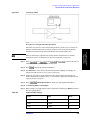
Do not exceed the operating input power, voltage, and current
level and signal type appropriate for the instrument being used, refer to
your instrument's Function Reference.
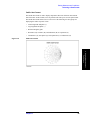
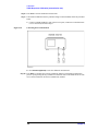
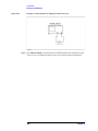
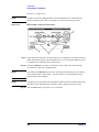
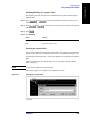
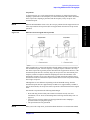
Electrostatic discharge(ESD) can damage the highly sensitive
microcircuits in your instrument. ESD damage is most likely to occur as
the test fixtures are being connected or disconnected. Protect them from
ESD damage by wearing a grounding strap that provides a high
resistance path to ground. Alternatively, ground yourself to discharge any
static charge built-up by touching the outer shell of any grounded
instrument chassis before touching the test port connectors.
Safety Summary
When you notice any of the unusual conditions listed below, immediately
terminate operation and disconnect the power cable.
Contact your local Agilent Technologies sales representative or
authorized service company for repair of the instrument. If you continue
to operate without repairing the instrument, there is a potential fire or
shock hazard for the operator.
- Instrument operates abnormally.
- Instrument emits abnormal noise, smell, smoke or a spark-like
light during operation.
- Instrument generates high temperature or electrical shock
during operation.
- Power cable, plug, or receptacle on instrument is damaged.
- Foreign substance or liquid has fallen into the instrument.
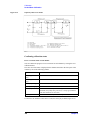
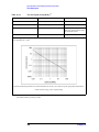
Herstellerbescheinigung
GERAUSCHEMISSION
LpA
< 70 dB
am Arbeitsplatz
normaler Betrieb
nach DIN 45635 T. 19
Manufacturer's Declaration
ACOUSTIC NOISE EMISSION
LpA
< 70 dB
operator position
normal operation
per ISO 7779
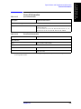
Regulatory compliance information
This product complies with the essential requirements of the following applicable European Directives, and
carries the CE marking accordingly:
The Low Voltage Directive 73/23/EEC, amended by 93/68/EEC
The EMC Directive 89/336/EEC, amended by 93/68/EEC
To obtain Declaration of Conformity, please contact your local Agilent Technologies sales office, agent or
distributor.
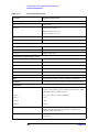
Safety notice supplement
・ This equipment complies with EN/IEC61010-1:2001.
・ This equipment is MEASUREMENT CATEGORY I (CAT I). Do not use for CAT II, III, or IV.
・ Do not connect the measuring terminals to mains.
・ This equipment is POLLUTION DEGREE 2, INDOOR USE product.
・ This equipment is tested with stand-alone condition or with the combination with the accessories supplied
by Agilent Technologies against the requirement of the standards described in the Declaration of
Conformity. If it is used as a system component, compliance of related regulations and safety requirements
are to be confirmed by the builder of the system.
Agilent E5070B/E5071B ENA Series RF Network Analyzers
User’s Guide
Eleventh Edition
FIRMWARE REVISIONS
This manual applies directly to instruments that have the firmware revision A.08.10.
For additional information about firmware revisions, see Appendix A.
Manufacturing No. E5070-90430
June 2007
Notices
The information contained in this document is subject to change without notice.
This document contains proprietary information that is protected by copyright. All rights
are reserved. No part of this document may be photocopied, reproduced, or translated to
another language without the prior written consent of Agilent Technologies.
Microsoft®,MS-DOS®,Windows®,Visual C++®,Visual Basic®,VBA® and Excel® are
registered
UNIX is a registered trademark in U.S. and other countries, licensed
exclusively through X/Open Company Limited.
Portions ©Copyright 1996, Microsoft Corporation. All rights reserved.
© Copyright 2002, 2003, 2004, 2005, 2006, 2007 Agilent Technologies
Manual Printing History
The manual’s printing date and part number indicate its current edition. The printing date
changes when a new edition is printed (minor corrections and updates that are incorporated
at reprint do not cause the date to change). The manual part number changes when
extensive technical changes are incorporated.
August 2002
First Edition (part number: E5070-90030)
March 2003
Second Edition (part number: E5070-90040, changes for firmware
version A.03.50)
July 2003
Third Edition (part number: E5070-90050)
January 2004
Fourth Edition (part number: E5070-90060, changes for firmware
version A.03.60)
March 2004
Fifth Edition (part number: E5070-90070)
August 2004
Sixth Edition (part number: E5070-90080, changes for firmware
version A.04.00)
May 2005
Seventh Edition (part number: E5070-90090, changes for firmware
version A.05.00)
November 2005
Eighth Edition (part number: E5070-90400, changes for firmware
version A.06.00)
May 2006
Ninth Edition (part number: E5070-90410, changes for firmware
version A.06.50)
February 2007
Tenth Edition (part number: E5070-90420, changes for firmware
version A.08.00)
June 2007
Eleventh Edition (part number: E5070-90430, changes for firmware
version A.08.10)
2
Safety Summary
The following general safety precautions must be observed during all phases of operation,
service, and repair of this instrument. Failure to comply with these precautions or with
specific WARNINGS elsewhere in this manual may impair the protection provided by the
equipment. Such noncompliance would also violate safety standards of design,
manufacture, and intended use of the instrument. Agilent Technologies assumes no liability
for the customer’s failure to comply with these precautions.
NOTE
The E5070B/E5071B complies with INSTALLATION CATEGORY II as well as
POLLUTION DEGREE 2 in IEC61010-1. The E5070B/E5071B is an INDOOR USE
product.
NOTE
The LEDs in the E5070B/E5071B are Class 1 in accordance with IEC60825-1,
CLASS 1 LED PRODUCT.
•
Ground the Instrument
To avoid electric shock, the instrument chassis and cabinet must be grounded with the
supplied power cable’s grounding prong.
•
DO NOT Operate in an Explosive Atmosphere
Do not operate the instrument in the presence of inflammable gasses or fumes.
Operation of any electrical instrument in such an environment clearly constitutes a
safety hazard.
•
Keep Away from Live Circuits
Operators must not remove instrument covers. Component replacement and internal
adjustments must be made by qualified maintenance personnel. Do not replace
components with the power cable connected. Under certain conditions, dangerous
voltage levels may remain even after the power cable has been disconnected. To avoid
injuries, always disconnect the power and discharge circuits before touching them.
•
DO NOT Service or Adjust the Instrument Alone
Do not attempt internal service or adjustment unless another person, capable of
rendering first aid and resuscitation, is present.
•
DO NOT Substitute Parts or Modify the Instrument
To avoid the danger of introducing additional hazards, do not install substitute parts or
perform unauthorized modifications to the instrument. Return the instrument to an
Agilent Technologies Sales and Service Office for service and repair to ensure that
safety features are maintained in operational condition.
•
Dangerous Procedure Warnings
Warnings, such as the example below, precede potentially dangerous procedures
throughout this manual. Instructions contained in the warnings must be followed.
WARNING
Dangerous voltage levels, capable of causing death, are present in this instrument.
Use extreme caution when handling, testing, and adjusting this instrument.
3
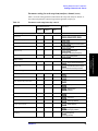
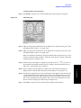
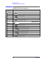
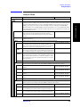
Safety Symbols
General definitions of safety symbols used on the instrument or in manuals are listed
below.
Instruction Manual symbol: the product is marked with this symbol when it is necessary for
the user to refer to the instrument manual.
Alternating current.
Direct current.
On (Supply).
Off (Supply).
In-position of push-button switch.
Out-position of push-button switch.
A chassis terminal; a connection to the instrument’s chassis, which includes all exposed
metal structure.
Stand-by.
WARNING
This warning sign denotes a hazard. It calls attention to a procedure, practice, or
condition that, if not correctly performed or adhered to, could result in injury or
death to personnel.
CAUTION
This Caution sign denotes a hazard. It calls attention to a procedure, practice, or condition
that, if not correctly performed or adhered to, could result in damage to or destruction of
part or all of the instrument.
NOTE
This Note sign denotes important information. It calls attention to a procedure, practice, or
condition that is essential for the user to understand.
4
Certification
Agilent Technologies certifies that this product met its published specifications at the time
of shipment from the factory. Agilent Technologies further certifies that its calibration
measurements are traceable to the United States National Institute of Standards and
Technology, to the extent allowed by the Institution’s calibration facility or by the
calibration facilities of other International Standards Organization members.
Documentation Warranty
The material contained in this document is provided "as is," and is subject to being
changed, without notice, in future editions. Further, to the maximum extent permitted by
applicable law, Agilent disclaims all warranties, either express or implied with regard to
this manual and any information contained herein, including but not limited to the implied
warranties of merchantability and fitness for a particular purpose. Agilent shall not be
liable for errors or for incidental or consequential damages in connection with the
furnishing, use, or performance of this document or any information contained herein.
Should Agilent and the user have a separate written agreement with warranty terms
covering the material in this document that conflict with these terms, the warranty terms in
the separate agreement will control.
Exclusive Remedies
The remedies provided herein are Buyer’s sole and exclusive remedies. Agilent
Technologies shall not be liable for any direct, indirect, special, incidental, or
consequential damages, whether based on contract, tort, or any other legal theory.
Assistance
Product maintenance agreements and other customer assistance agreements are available
for Agilent Technologies products.
For any assistance, contact your nearest Agilent Technologies Sales and Service Office.
Addresses are provided at the back of this manual.
5
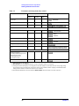
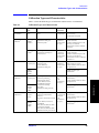
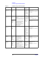
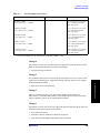
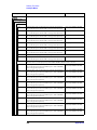
Typeface Conventions
Sample (bold)
Boldface type is used when a term is defined or
emphasis.
Sample (Italic)
Italic type is used for emphasis.
key
Indicates a hardkey (key on the front panel or
external keyboard) labeled “Sample.” “key” may
be omitted.
Sample menu/button/box
Indicates a menu/button/box on the screen labeled
“Sample” which can be selected/executed by
clicking. “menu,” “button,” or “box” may be
omitted.
Sample block/toolbar
Indicates a block (group of hardkeys) or a toolbar
(setup toolbar) labeled “Sample.”
Sample 1 - Sample 2 - Sample 3
Indicates a sequential operation of Sample 1,
Sample 2, and Sample 3 (menu, button, or box).
“-” may be omitted.
6
Documentation Map
The following manuals are available for the Agilent E5070B/E5071B.
•
User’s Guide (Part Number E5070-904x0, attached to Option ABA)
This manual describes most of the basic information needed to use the
E5070B/E5071B. It provides a function overview, detailed operation procedure for
each function (from preparation for measurement to analysis of measurement results),
measurement examples, specifications, and supplemental information. For
programming guidance on performing automatic measurement with the
E5070B/E5071B, please see the Programming Manual.
•
Installation and Quick Start Guide (Part Number E5070-900x1, attached to Option
ABA)
This manual describes installation of the instrument after it is delivered and the basic
procedures for applications and analysis. Refer to this manual when you use the
E5070B/E5071B for the first time.
•
Programmer’s Guide (Part Number E5070-900x2, attached to Option ABA)
This manual provides programming information for performing automatic
measurement with the E5070B/E5071B. It includes an outline of remote control,
procedures for detecting measurement start (trigger) and end (sweep end), application
programming examples, a command reference, and related information.
•
VBA Programmer’s Guide (Part Number E5070-900x3, attached to Option ABA)
This manual describes programming information for performing automatic
measurement with internal controller. It includes an outline of VBA programming,
some sample programming examples, a COM object reference, and related
information.
NOTE
The number position shown by “x” in the part numbers above indicates the edition number.
This convention is applied to each manual, CD-ROM (for manuals), and sample programs
disk issued.
7
VBA Macro
The Agilent folder (D:\Agilent) on the hard disk of the E5070B/E5071B contains the VBA
macros (VBA Projects) used in this manual.
The customer shall have the personal, non-transferable rights to use, copy, or modify the
VBA macros for the customer’s internal operations.
The customer shall use the VBA macros solely and exclusively for their own purposes and
shall not license, lease, market, or distribute the VBA macros or modification of any part
thereof.
Agilent Technologies shall not be liable for any infringement of any patent, trademark,
copyright, or other proprietary right by the VBA macros or their use. Agilent Technologies
does not warrant that the VBA macros are free from infringements of such rights of third
parties. However, Agilent Technologies will not knowingly infringe or deliver software
that infringes the patent, trademark, copyright, or other proprietary right of a third party.
8
Contents
1. Precautions
Software Installed . . . . . . . . . . . . . . . . . . . . . . . . . . . . . . . . . . . . . . . . . . . . . . . . . . . . . . . . . . . . . . . . . . . . . 26
Before contacting us . . . . . . . . . . . . . . . . . . . . . . . . . . . . . . . . . . . . . . . . . . . . . . . . . . . . . . . . . . . . . . . . . . . 27
2. Overview of Functions
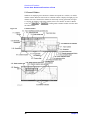
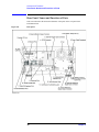
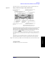
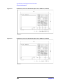
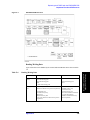
Front Panel: Names and Functions of Parts . . . . . . . . . . . . . . . . . . . . . . . . . . . . . . . . . . . . . . . . . . . . . . . . . 30
1. Standby Switch . . . . . . . . . . . . . . . . . . . . . . . . . . . . . . . . . . . . . . . . . . . . . . . . . . . . . . . . . . . . . . . . . . . 31
2. LCD Screen . . . . . . . . . . . . . . . . . . . . . . . . . . . . . . . . . . . . . . . . . . . . . . . . . . . . . . . . . . . . . . . . . . . . . . 31
3. ACTIVE CH/TRACE Block. . . . . . . . . . . . . . . . . . . . . . . . . . . . . . . . . . . . . . . . . . . . . . . . . . . . . . . . . 32
4. RESPONSE Block . . . . . . . . . . . . . . . . . . . . . . . . . . . . . . . . . . . . . . . . . . . . . . . . . . . . . . . . . . . . . . . . 33
5. STIMULUS Block . . . . . . . . . . . . . . . . . . . . . . . . . . . . . . . . . . . . . . . . . . . . . . . . . . . . . . . . . . . . . . . . 34
6. Floppy Disk Drive. . . . . . . . . . . . . . . . . . . . . . . . . . . . . . . . . . . . . . . . . . . . . . . . . . . . . . . . . . . . . . . . . 34
7. NAVIGATION Block . . . . . . . . . . . . . . . . . . . . . . . . . . . . . . . . . . . . . . . . . . . . . . . . . . . . . . . . . . . . . . 35
8. ENTRY Block . . . . . . . . . . . . . . . . . . . . . . . . . . . . . . . . . . . . . . . . . . . . . . . . . . . . . . . . . . . . . . . . . . . . 36
9. INSTR STATE Block . . . . . . . . . . . . . . . . . . . . . . . . . . . . . . . . . . . . . . . . . . . . . . . . . . . . . . . . . . . . . . 37
10. MKR/ANALYSIS Block. . . . . . . . . . . . . . . . . . . . . . . . . . . . . . . . . . . . . . . . . . . . . . . . . . . . . . . . . . . 38
11. Test Port. . . . . . . . . . . . . . . . . . . . . . . . . . . . . . . . . . . . . . . . . . . . . . . . . . . . . . . . . . . . . . . . . . . . . . . . 38
12. Front USB Port . . . . . . . . . . . . . . . . . . . . . . . . . . . . . . . . . . . . . . . . . . . . . . . . . . . . . . . . . . . . . . . . . . 39
13. Ground Terminal . . . . . . . . . . . . . . . . . . . . . . . . . . . . . . . . . . . . . . . . . . . . . . . . . . . . . . . . . . . . . . . . . 39
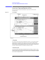
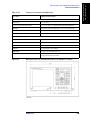
Screen Area: Names and Functions of Parts. . . . . . . . . . . . . . . . . . . . . . . . . . . . . . . . . . . . . . . . . . . . . . . . . 40
1. Menu Bar. . . . . . . . . . . . . . . . . . . . . . . . . . . . . . . . . . . . . . . . . . . . . . . . . . . . . . . . . . . . . . . . . . . . . . . . 40
2. Data Entry Bar. . . . . . . . . . . . . . . . . . . . . . . . . . . . . . . . . . . . . . . . . . . . . . . . . . . . . . . . . . . . . . . . . . . . 40
3. Softkey Menu Bar . . . . . . . . . . . . . . . . . . . . . . . . . . . . . . . . . . . . . . . . . . . . . . . . . . . . . . . . . . . . . . . . . 42
4. Instrument Status Bar . . . . . . . . . . . . . . . . . . . . . . . . . . . . . . . . . . . . . . . . . . . . . . . . . . . . . . . . . . . . . . 44
5. Channel Window . . . . . . . . . . . . . . . . . . . . . . . . . . . . . . . . . . . . . . . . . . . . . . . . . . . . . . . . . . . . . . . . . . 46
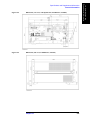
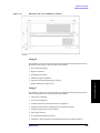
Rear Panel: Names and Functions of Parts . . . . . . . . . . . . . . . . . . . . . . . . . . . . . . . . . . . . . . . . . . . . . . . . . . 54
1. Handler I/O Port . . . . . . . . . . . . . . . . . . . . . . . . . . . . . . . . . . . . . . . . . . . . . . . . . . . . . . . . . . . . . . . . . . 55
2. Ethernet Port . . . . . . . . . . . . . . . . . . . . . . . . . . . . . . . . . . . . . . . . . . . . . . . . . . . . . . . . . . . . . . . . . . . . . 55
3. External Monitor Output Terminal (Video). . . . . . . . . . . . . . . . . . . . . . . . . . . . . . . . . . . . . . . . . . . . . . 55
4. GPIB Connector . . . . . . . . . . . . . . . . . . . . . . . . . . . . . . . . . . . . . . . . . . . . . . . . . . . . . . . . . . . . . . . . . . 55
5. External Trigger Input Connector (Ext Trig) . . . . . . . . . . . . . . . . . . . . . . . . . . . . . . . . . . . . . . . . . . . . 55
6. Fan. . . . . . . . . . . . . . . . . . . . . . . . . . . . . . . . . . . . . . . . . . . . . . . . . . . . . . . . . . . . . . . . . . . . . . . . . . . . . 55
7. Line Switch (Always ON). . . . . . . . . . . . . . . . . . . . . . . . . . . . . . . . . . . . . . . . . . . . . . . . . . . . . . . . . . . 55
8. Power Cable Receptacle (to LINE) . . . . . . . . . . . . . . . . . . . . . . . . . . . . . . . . . . . . . . . . . . . . . . . . . . . . 56
9. High Stability Frequency Reference Output Connector (Ref Oven, Option 1E5 only) . . . . . . . . . . . . 56
10. External Reference Signal Input Connector (Ref In) . . . . . . . . . . . . . . . . . . . . . . . . . . . . . . . . . . . . . 56
11. Internal Reference Signal Output Connector (Ref Out) . . . . . . . . . . . . . . . . . . . . . . . . . . . . . . . . . . . 57
12. Serial Number Plate . . . . . . . . . . . . . . . . . . . . . . . . . . . . . . . . . . . . . . . . . . . . . . . . . . . . . . . . . . . . . . 57
13. Certificate of Authenticity Label. . . . . . . . . . . . . . . . . . . . . . . . . . . . . . . . . . . . . . . . . . . . . . . . . . . . . 57
14. Rear USB port . . . . . . . . . . . . . . . . . . . . . . . . . . . . . . . . . . . . . . . . . . . . . . . . . . . . . . . . . . . . . . . . . . . 57
15. Reserved Port (Reserved) . . . . . . . . . . . . . . . . . . . . . . . . . . . . . . . . . . . . . . . . . . . . . . . . . . . . . . . . . . 57
16. Printer Parallel Port . . . . . . . . . . . . . . . . . . . . . . . . . . . . . . . . . . . . . . . . . . . . . . . . . . . . . . . . . . . . . . . 57
17. Mini-DIN Keyboard Port . . . . . . . . . . . . . . . . . . . . . . . . . . . . . . . . . . . . . . . . . . . . . . . . . . . . . . . . . . 57
18. Mini-DIN Mouse Port . . . . . . . . . . . . . . . . . . . . . . . . . . . . . . . . . . . . . . . . . . . . . . . . . . . . . . . . . . . . . 58
19. USB (USBTMC) Interface Port . . . . . . . . . . . . . . . . . . . . . . . . . . . . . . . . . . . . . . . . . . . . . . . . . . . . . 58
3. Setting Measurement Conditions
Initializing Parameters . . . . . . . . . . . . . . . . . . . . . . . . . . . . . . . . . . . . . . . . . . . . . . . . . . . . . . . . . . . . . . . . . 60
9
Contents
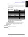
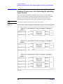
Setting Channels and Traces. . . . . . . . . . . . . . . . . . . . . . . . . . . . . . . . . . . . . . . . . . . . . . . . . . . . . . . . . . . . .
Setting upper limits of number of channels/traces . . . . . . . . . . . . . . . . . . . . . . . . . . . . . . . . . . . . . . . . . .
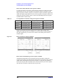
Setting channel display (layout of channel windows) . . . . . . . . . . . . . . . . . . . . . . . . . . . . . . . . . . . . . . .
Setting trace display . . . . . . . . . . . . . . . . . . . . . . . . . . . . . . . . . . . . . . . . . . . . . . . . . . . . . . . . . . . . . . . . .
Active channel . . . . . . . . . . . . . . . . . . . . . . . . . . . . . . . . . . . . . . . . . . . . . . . . . . . . . . . . . . . . . . . . . . . . .
Active trace . . . . . . . . . . . . . . . . . . . . . . . . . . . . . . . . . . . . . . . . . . . . . . . . . . . . . . . . . . . . . . . . . . . . . . . .
Parameter setting for each setup item (analyzer, channel, trace) . . . . . . . . . . . . . . . . . . . . . . . . . . . . . . .
Setting the System Z0. . . . . . . . . . . . . . . . . . . . . . . . . . . . . . . . . . . . . . . . . . . . . . . . . . . . . . . . . . . . . . . . . .
Setting Stimulus Conditions . . . . . . . . . . . . . . . . . . . . . . . . . . . . . . . . . . . . . . . . . . . . . . . . . . . . . . . . . . . . .
Setting sweep type . . . . . . . . . . . . . . . . . . . . . . . . . . . . . . . . . . . . . . . . . . . . . . . . . . . . . . . . . . . . . . . . . .
Setting the Sweep Range . . . . . . . . . . . . . . . . . . . . . . . . . . . . . . . . . . . . . . . . . . . . . . . . . . . . . . . . . . . . .
Turning stimulus signal output on/off. . . . . . . . . . . . . . . . . . . . . . . . . . . . . . . . . . . . . . . . . . . . . . . . . . . .
Setting fixed frequency at power sweep . . . . . . . . . . . . . . . . . . . . . . . . . . . . . . . . . . . . . . . . . . . . . . . . . .
Setting power level with Auto Power Range set function . . . . . . . . . . . . . . . . . . . . . . . . . . . . . . . . . . . .
Setting power range manually . . . . . . . . . . . . . . . . . . . . . . . . . . . . . . . . . . . . . . . . . . . . . . . . . . . . . . . . .
Setting the number of points . . . . . . . . . . . . . . . . . . . . . . . . . . . . . . . . . . . . . . . . . . . . . . . . . . . . . . . . . . .
Setting the sweep time . . . . . . . . . . . . . . . . . . . . . . . . . . . . . . . . . . . . . . . . . . . . . . . . . . . . . . . . . . . . . . .
Selecting Measurement Parameters . . . . . . . . . . . . . . . . . . . . . . . . . . . . . . . . . . . . . . . . . . . . . . . . . . . . . . .
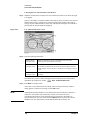
Definition of S-parameters . . . . . . . . . . . . . . . . . . . . . . . . . . . . . . . . . . . . . . . . . . . . . . . . . . . . . . . . . . . .
Setting up S-parameters . . . . . . . . . . . . . . . . . . . . . . . . . . . . . . . . . . . . . . . . . . . . . . . . . . . . . . . . . . . . . .
Selecting a Data Format . . . . . . . . . . . . . . . . . . . . . . . . . . . . . . . . . . . . . . . . . . . . . . . . . . . . . . . . . . . . . . . .
Rectangular display formats . . . . . . . . . . . . . . . . . . . . . . . . . . . . . . . . . . . . . . . . . . . . . . . . . . . . . . . . . . .
Polar format . . . . . . . . . . . . . . . . . . . . . . . . . . . . . . . . . . . . . . . . . . . . . . . . . . . . . . . . . . . . . . . . . . . . . . .
Smith chart format . . . . . . . . . . . . . . . . . . . . . . . . . . . . . . . . . . . . . . . . . . . . . . . . . . . . . . . . . . . . . . . . . .
Selecting a data format . . . . . . . . . . . . . . . . . . . . . . . . . . . . . . . . . . . . . . . . . . . . . . . . . . . . . . . . . . . . . . .
Setting the Scales . . . . . . . . . . . . . . . . . . . . . . . . . . . . . . . . . . . . . . . . . . . . . . . . . . . . . . . . . . . . . . . . . . . . .
Auto scale . . . . . . . . . . . . . . . . . . . . . . . . . . . . . . . . . . . . . . . . . . . . . . . . . . . . . . . . . . . . . . . . . . . . . . . . .
Manual scale adjustment on a rectangular display format . . . . . . . . . . . . . . . . . . . . . . . . . . . . . . . . . . . .
Manual scale adjustment on the Smith chart/polar format . . . . . . . . . . . . . . . . . . . . . . . . . . . . . . . . . . . .
Setting the value of a reference line using the marker . . . . . . . . . . . . . . . . . . . . . . . . . . . . . . . . . . . . . . .
Setting Window Displays . . . . . . . . . . . . . . . . . . . . . . . . . . . . . . . . . . . . . . . . . . . . . . . . . . . . . . . . . . . . . . .
Maximizing the specified window/trace display . . . . . . . . . . . . . . . . . . . . . . . . . . . . . . . . . . . . . . . . . . .
Turning off the display of graticule labels . . . . . . . . . . . . . . . . . . . . . . . . . . . . . . . . . . . . . . . . . . . . . . . .
Hiding Frequency Information . . . . . . . . . . . . . . . . . . . . . . . . . . . . . . . . . . . . . . . . . . . . . . . . . . . . . . . . .
Labeling a window . . . . . . . . . . . . . . . . . . . . . . . . . . . . . . . . . . . . . . . . . . . . . . . . . . . . . . . . . . . . . . . . . .
Setting display colors . . . . . . . . . . . . . . . . . . . . . . . . . . . . . . . . . . . . . . . . . . . . . . . . . . . . . . . . . . . . . . . .
61
61
62
64
66
66
67
69
70
70
70
73
73
74
77
78
78
80
80
80
81
81
82
83
84
85
85
85
87
87
88
88
88
89
89
91
4. Calibration
Measurement Errors and their Characteristics . . . . . . . . . . . . . . . . . . . . . . . . . . . . . . . . . . . . . . . . . . . . . . . 94
Drift Errors . . . . . . . . . . . . . . . . . . . . . . . . . . . . . . . . . . . . . . . . . . . . . . . . . . . . . . . . . . . . . . . . . . . . . . . . 94
Random Errors . . . . . . . . . . . . . . . . . . . . . . . . . . . . . . . . . . . . . . . . . . . . . . . . . . . . . . . . . . . . . . . . . . . . . 94
Systematic Errors . . . . . . . . . . . . . . . . . . . . . . . . . . . . . . . . . . . . . . . . . . . . . . . . . . . . . . . . . . . . . . . . . . . 95
Calibration Types and Characteristics . . . . . . . . . . . . . . . . . . . . . . . . . . . . . . . . . . . . . . . . . . . . . . . . . . . . . 99
Checking Calibration Status . . . . . . . . . . . . . . . . . . . . . . . . . . . . . . . . . . . . . . . . . . . . . . . . . . . . . . . . . . . . 102
Execution status of error correction for each channel . . . . . . . . . . . . . . . . . . . . . . . . . . . . . . . . . . . . . . 102
Execution status of error correction for each trace . . . . . . . . . . . . . . . . . . . . . . . . . . . . . . . . . . . . . . . . . 102
Acquisition status of calibration coefficient for each channel . . . . . . . . . . . . . . . . . . . . . . . . . . . . . . . . 103
Selecting Calibration Kit . . . . . . . . . . . . . . . . . . . . . . . . . . . . . . . . . . . . . . . . . . . . . . . . . . . . . . . . . . . . . . 105
Setting the trigger source for calibration . . . . . . . . . . . . . . . . . . . . . . . . . . . . . . . . . . . . . . . . . . . . . . . . . . 106
10
Contents
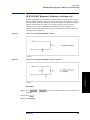
OPEN/SHORT Response Calibration (reflection test) . . . . . . . . . . . . . . . . . . . . . . . . . . . . . . . . . . . . . . . . 107
Procedure. . . . . . . . . . . . . . . . . . . . . . . . . . . . . . . . . . . . . . . . . . . . . . . . . . . . . . . . . . . . . . . . . . . . . . . . . 107
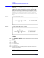
THRU Response Calibration (transmission test) . . . . . . . . . . . . . . . . . . . . . . . . . . . . . . . . . . . . . . . . . . . . 110
Procedure. . . . . . . . . . . . . . . . . . . . . . . . . . . . . . . . . . . . . . . . . . . . . . . . . . . . . . . . . . . . . . . . . . . . . . . . . 110
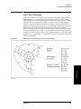
1-Port Calibration (reflection test) . . . . . . . . . . . . . . . . . . . . . . . . . . . . . . . . . . . . . . . . . . . . . . . . . . . . . . . 113
Procedure. . . . . . . . . . . . . . . . . . . . . . . . . . . . . . . . . . . . . . . . . . . . . . . . . . . . . . . . . . . . . . . . . . . . . . . . . 114
Enhanced Response Calibration . . . . . . . . . . . . . . . . . . . . . . . . . . . . . . . . . . . . . . . . . . . . . . . . . . . . . . . . . 115
Procedure. . . . . . . . . . . . . . . . . . . . . . . . . . . . . . . . . . . . . . . . . . . . . . . . . . . . . . . . . . . . . . . . . . . . . . . . . 116
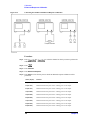
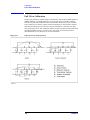
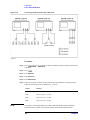
Full 2-Port Calibration . . . . . . . . . . . . . . . . . . . . . . . . . . . . . . . . . . . . . . . . . . . . . . . . . . . . . . . . . . . . . . . . 118
Procedure. . . . . . . . . . . . . . . . . . . . . . . . . . . . . . . . . . . . . . . . . . . . . . . . . . . . . . . . . . . . . . . . . . . . . . . . . 119
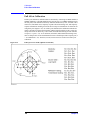
Full 3-Port Calibration . . . . . . . . . . . . . . . . . . . . . . . . . . . . . . . . . . . . . . . . . . . . . . . . . . . . . . . . . . . . . . . . 121
Procedure. . . . . . . . . . . . . . . . . . . . . . . . . . . . . . . . . . . . . . . . . . . . . . . . . . . . . . . . . . . . . . . . . . . . . . . . . 122
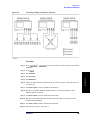
Full 4-Port Calibration . . . . . . . . . . . . . . . . . . . . . . . . . . . . . . . . . . . . . . . . . . . . . . . . . . . . . . . . . . . . . . . . 124
Procedure. . . . . . . . . . . . . . . . . . . . . . . . . . . . . . . . . . . . . . . . . . . . . . . . . . . . . . . . . . . . . . . . . . . . . . . . . 125
ECal (electronic calibration) . . . . . . . . . . . . . . . . . . . . . . . . . . . . . . . . . . . . . . . . . . . . . . . . . . . . . . . . . . . . 127
1-Port Calibration Using a 2-Port ECal Module . . . . . . . . . . . . . . . . . . . . . . . . . . . . . . . . . . . . . . . . . . . 127
Full 2-Port Calibration Using the 2-Port ECal Module. . . . . . . . . . . . . . . . . . . . . . . . . . . . . . . . . . . . . . 128
Unknown Thru Calibration . . . . . . . . . . . . . . . . . . . . . . . . . . . . . . . . . . . . . . . . . . . . . . . . . . . . . . . . . . . 130
Turning off ECal auto-detect function . . . . . . . . . . . . . . . . . . . . . . . . . . . . . . . . . . . . . . . . . . . . . . . . . . 131
Full 3-Port and Full 4-Port Calibration using 2-Port ECal . . . . . . . . . . . . . . . . . . . . . . . . . . . . . . . . . . . . . 132
Operational procedure . . . . . . . . . . . . . . . . . . . . . . . . . . . . . . . . . . . . . . . . . . . . . . . . . . . . . . . . . . . . . . . 132
Calibration Using 4-port ECal . . . . . . . . . . . . . . . . . . . . . . . . . . . . . . . . . . . . . . . . . . . . . . . . . . . . . . . . . . 135
Operational procedure . . . . . . . . . . . . . . . . . . . . . . . . . . . . . . . . . . . . . . . . . . . . . . . . . . . . . . . . . . . . . . . 135
2-port TRL calibration . . . . . . . . . . . . . . . . . . . . . . . . . . . . . . . . . . . . . . . . . . . . . . . . . . . . . . . . . . . . . . . . 137
Operational procedure . . . . . . . . . . . . . . . . . . . . . . . . . . . . . . . . . . . . . . . . . . . . . . . . . . . . . . . . . . . . . . . 138
3-port TRL calibration . . . . . . . . . . . . . . . . . . . . . . . . . . . . . . . . . . . . . . . . . . . . . . . . . . . . . . . . . . . . . . . . 140
Operational procedure . . . . . . . . . . . . . . . . . . . . . . . . . . . . . . . . . . . . . . . . . . . . . . . . . . . . . . . . . . . . . . . 141
4-port TRL calibration . . . . . . . . . . . . . . . . . . . . . . . . . . . . . . . . . . . . . . . . . . . . . . . . . . . . . . . . . . . . . . . . 144
Operational procedure . . . . . . . . . . . . . . . . . . . . . . . . . . . . . . . . . . . . . . . . . . . . . . . . . . . . . . . . . . . . . . . 145
Simplified calibration . . . . . . . . . . . . . . . . . . . . . . . . . . . . . . . . . . . . . . . . . . . . . . . . . . . . . . . . . . . . . . . . . 148
Simplified full 3/4-port calibration . . . . . . . . . . . . . . . . . . . . . . . . . . . . . . . . . . . . . . . . . . . . . . . . . . . . . 148
Simplified 3/4-port TRL calibration . . . . . . . . . . . . . . . . . . . . . . . . . . . . . . . . . . . . . . . . . . . . . . . . . . . . 149
Partial overwrite . . . . . . . . . . . . . . . . . . . . . . . . . . . . . . . . . . . . . . . . . . . . . . . . . . . . . . . . . . . . . . . . . . . . . 151
Procedure. . . . . . . . . . . . . . . . . . . . . . . . . . . . . . . . . . . . . . . . . . . . . . . . . . . . . . . . . . . . . . . . . . . . . . . . . 151
Improving accuracy of measurement using partial overwrite (thru calibration) along with ECal . . . . . 152
Unknown Thru Calibration . . . . . . . . . . . . . . . . . . . . . . . . . . . . . . . . . . . . . . . . . . . . . . . . . . . . . . . . . . . . . 153
Procedure. . . . . . . . . . . . . . . . . . . . . . . . . . . . . . . . . . . . . . . . . . . . . . . . . . . . . . . . . . . . . . . . . . . . . . . . . 153
Calibration between Ports of Different Connector Types. . . . . . . . . . . . . . . . . . . . . . . . . . . . . . . . . . . . . . 155
Operating procedure . . . . . . . . . . . . . . . . . . . . . . . . . . . . . . . . . . . . . . . . . . . . . . . . . . . . . . . . . . . . . . . . 156
Adapter Characterization . . . . . . . . . . . . . . . . . . . . . . . . . . . . . . . . . . . . . . . . . . . . . . . . . . . . . . . . . . . . . . 160
Concept . . . . . . . . . . . . . . . . . . . . . . . . . . . . . . . . . . . . . . . . . . . . . . . . . . . . . . . . . . . . . . . . . . . . . . . . . . 161
How to execute adapter characterization . . . . . . . . . . . . . . . . . . . . . . . . . . . . . . . . . . . . . . . . . . . . . . . . 162
Execution procedure of characterization for test fixture using probe . . . . . . . . . . . . . . . . . . . . . . . . . . . 165
Adapter Removal-Insertion. . . . . . . . . . . . . . . . . . . . . . . . . . . . . . . . . . . . . . . . . . . . . . . . . . . . . . . . . . . . . 167
About Adapter Removal . . . . . . . . . . . . . . . . . . . . . . . . . . . . . . . . . . . . . . . . . . . . . . . . . . . . . . . . . . . . . 167
About Adapter Insertion . . . . . . . . . . . . . . . . . . . . . . . . . . . . . . . . . . . . . . . . . . . . . . . . . . . . . . . . . . . . . 169
Procedure for Adapter Removal / Insertion . . . . . . . . . . . . . . . . . . . . . . . . . . . . . . . . . . . . . . . . . . . . . . 170
User-characterized ECal . . . . . . . . . . . . . . . . . . . . . . . . . . . . . . . . . . . . . . . . . . . . . . . . . . . . . . . . . . . . . . . 171
Precautions to take in using VBA macros. . . . . . . . . . . . . . . . . . . . . . . . . . . . . . . . . . . . . . . . . . . . . . . . 171
11
Contents
Storing user characteristics to the ECal module . . . . . . . . . . . . . . . . . . . . . . . . . . . . . . . . . . . . . . . . . . .
Backup and recovery of ECal module's built-in flash memory . . . . . . . . . . . . . . . . . . . . . . . . . . . . . . .
Executing User-characterized ECal . . . . . . . . . . . . . . . . . . . . . . . . . . . . . . . . . . . . . . . . . . . . . . . . . . . .
Confidence Check on Calibration Coefficients Using ECal . . . . . . . . . . . . . . . . . . . . . . . . . . . . . . . . . . .
Operational procedure. . . . . . . . . . . . . . . . . . . . . . . . . . . . . . . . . . . . . . . . . . . . . . . . . . . . . . . . . . . . . . .
Changing the Calibration Kit Definition . . . . . . . . . . . . . . . . . . . . . . . . . . . . . . . . . . . . . . . . . . . . . . . . . .
Definitions of terms . . . . . . . . . . . . . . . . . . . . . . . . . . . . . . . . . . . . . . . . . . . . . . . . . . . . . . . . . . . . . . . .
Defining parameters for standards . . . . . . . . . . . . . . . . . . . . . . . . . . . . . . . . . . . . . . . . . . . . . . . . . . . . .
Redefining a calibration kit. . . . . . . . . . . . . . . . . . . . . . . . . . . . . . . . . . . . . . . . . . . . . . . . . . . . . . . . . . .
Example of defining the TRL calibration kit . . . . . . . . . . . . . . . . . . . . . . . . . . . . . . . . . . . . . . . . . . . . .
Setting options for TRL calibration . . . . . . . . . . . . . . . . . . . . . . . . . . . . . . . . . . . . . . . . . . . . . . . . . . . .
Setting a media type for the calibration kit. . . . . . . . . . . . . . . . . . . . . . . . . . . . . . . . . . . . . . . . . . . . . . .
Saving and loading definition file of calibration kit . . . . . . . . . . . . . . . . . . . . . . . . . . . . . . . . . . . . . . . .
Default settings of pre-defined calibration kits. . . . . . . . . . . . . . . . . . . . . . . . . . . . . . . . . . . . . . . . . . . .
Specifying Different Standard for Each Frequency . . . . . . . . . . . . . . . . . . . . . . . . . . . . . . . . . . . . . . . . . .
Defining different standard for each frequency band . . . . . . . . . . . . . . . . . . . . . . . . . . . . . . . . . . . . . . .
Defining standard for each subclass . . . . . . . . . . . . . . . . . . . . . . . . . . . . . . . . . . . . . . . . . . . . . . . . . . . .
Disabling standard defined for a subclass. . . . . . . . . . . . . . . . . . . . . . . . . . . . . . . . . . . . . . . . . . . . . . . .
Notes on how frequency ranges are dealt when using subclasses . . . . . . . . . . . . . . . . . . . . . . . . . . . . .
Power Calibration. . . . . . . . . . . . . . . . . . . . . . . . . . . . . . . . . . . . . . . . . . . . . . . . . . . . . . . . . . . . . . . . . . . .
Turning ON or OFF power level error correction. . . . . . . . . . . . . . . . . . . . . . . . . . . . . . . . . . . . . . . . . .
Preparing power meter and sensor . . . . . . . . . . . . . . . . . . . . . . . . . . . . . . . . . . . . . . . . . . . . . . . . . . . . .
Selecting target port of error correction . . . . . . . . . . . . . . . . . . . . . . . . . . . . . . . . . . . . . . . . . . . . . . . . .
Setting loss compensation. . . . . . . . . . . . . . . . . . . . . . . . . . . . . . . . . . . . . . . . . . . . . . . . . . . . . . . . . . . .
Setting a tolerance for power calibration . . . . . . . . . . . . . . . . . . . . . . . . . . . . . . . . . . . . . . . . . . . . . . . .
Measuring calibration data . . . . . . . . . . . . . . . . . . . . . . . . . . . . . . . . . . . . . . . . . . . . . . . . . . . . . . . . . . .
Receiver Calibration. . . . . . . . . . . . . . . . . . . . . . . . . . . . . . . . . . . . . . . . . . . . . . . . . . . . . . . . . . . . . . . . . .
Turning ON/OFF receiver error correction. . . . . . . . . . . . . . . . . . . . . . . . . . . . . . . . . . . . . . . . . . . . . . .
Selecting target port for error correction . . . . . . . . . . . . . . . . . . . . . . . . . . . . . . . . . . . . . . . . . . . . . . . .
Measuring the calibration data . . . . . . . . . . . . . . . . . . . . . . . . . . . . . . . . . . . . . . . . . . . . . . . . . . . . . . . .
Vector-Mixer Calibration . . . . . . . . . . . . . . . . . . . . . . . . . . . . . . . . . . . . . . . . . . . . . . . . . . . . . . . . . . . . . .
Overview of vector-mixer calibration. . . . . . . . . . . . . . . . . . . . . . . . . . . . . . . . . . . . . . . . . . . . . . . . . . .
Measured mixer . . . . . . . . . . . . . . . . . . . . . . . . . . . . . . . . . . . . . . . . . . . . . . . . . . . . . . . . . . . . . . . . . . .
Calibration mixer (with IF filter) . . . . . . . . . . . . . . . . . . . . . . . . . . . . . . . . . . . . . . . . . . . . . . . . . . . . . .
Characterizing calibration mixer (with IF filter) . . . . . . . . . . . . . . . . . . . . . . . . . . . . . . . . . . . . . . . . . .
Characterizing procedure for calibration mixer (with IF filter) . . . . . . . . . . . . . . . . . . . . . . . . . . . . . . .
How to execute characterization of calibration mixer . . . . . . . . . . . . . . . . . . . . . . . . . . . . . . . . . . . . . .
Characterizing calibration mixer (with IF filter) for balance mixer measurement. . . . . . . . . . . . . . . . .
How to execute characterization. . . . . . . . . . . . . . . . . . . . . . . . . . . . . . . . . . . . . . . . . . . . . . . . . . . . . . .
Scalar-Mixer Calibration . . . . . . . . . . . . . . . . . . . . . . . . . . . . . . . . . . . . . . . . . . . . . . . . . . . . . . . . . . . . . .
Confirming calibration status . . . . . . . . . . . . . . . . . . . . . . . . . . . . . . . . . . . . . . . . . . . . . . . . . . . . . . . . .
Operational Procedure (when using mechanical calibration kit) . . . . . . . . . . . . . . . . . . . . . . . . . . . . . .
Operational procedure (when using ECal module). . . . . . . . . . . . . . . . . . . . . . . . . . . . . . . . . . . . . . . . .
172
176
177
179
179
181
182
183
185
188
190
191
192
193
202
202
203
204
205
208
208
209
215
215
218
218
220
220
221
221
223
223
224
224
224
225
226
230
230
233
234
235
238
5. Making Measurements
Setting Up the Trigger and Making Measurements . . . . . . . . . . . . . . . . . . . . . . . . . . . . . . . . . . . . . . . . . .
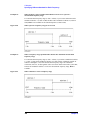
Sweep Order in Each Channel . . . . . . . . . . . . . . . . . . . . . . . . . . . . . . . . . . . . . . . . . . . . . . . . . . . . . . . .
Trigger Source. . . . . . . . . . . . . . . . . . . . . . . . . . . . . . . . . . . . . . . . . . . . . . . . . . . . . . . . . . . . . . . . . . . . .
Trigger Modes. . . . . . . . . . . . . . . . . . . . . . . . . . . . . . . . . . . . . . . . . . . . . . . . . . . . . . . . . . . . . . . . . . . . .
242
242
243
243
12
Contents
Setting Up the Trigger and Making Measurements . . . . . . . . . . . . . . . . . . . . . . . . . . . . . . . . . . . . . . . . 243
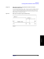
Setting the Point Trigger . . . . . . . . . . . . . . . . . . . . . . . . . . . . . . . . . . . . . . . . . . . . . . . . . . . . . . . . . . . . . . . 245
Procedure to Set the Point Trigger . . . . . . . . . . . . . . . . . . . . . . . . . . . . . . . . . . . . . . . . . . . . . . . . . . . . . 245
Setting the low-latency external trigger mode . . . . . . . . . . . . . . . . . . . . . . . . . . . . . . . . . . . . . . . . . . . . . . 246
Procedure to set the low-latency external trigger . . . . . . . . . . . . . . . . . . . . . . . . . . . . . . . . . . . . . . . . . . 246
External trigger delay time and point trigger interval . . . . . . . . . . . . . . . . . . . . . . . . . . . . . . . . . . . . . . . 247
Setting the Averaging Trigger Function . . . . . . . . . . . . . . . . . . . . . . . . . . . . . . . . . . . . . . . . . . . . . . . . . . . 249
Using the averaging trigger function. . . . . . . . . . . . . . . . . . . . . . . . . . . . . . . . . . . . . . . . . . . . . . . . . . . . 249
Executing a Trigger Only for Active Channel . . . . . . . . . . . . . . . . . . . . . . . . . . . . . . . . . . . . . . . . . . . . . . 250
Procedure to set the range . . . . . . . . . . . . . . . . . . . . . . . . . . . . . . . . . . . . . . . . . . . . . . . . . . . . . . . . . . . . 250
6. Data Analysis
Analyzing Data on the Trace Using the Marker . . . . . . . . . . . . . . . . . . . . . . . . . . . . . . . . . . . . . . . . . . . . . 252
About marker functions. . . . . . . . . . . . . . . . . . . . . . . . . . . . . . . . . . . . . . . . . . . . . . . . . . . . . . . . . . . . . . 252
Reading values on the trace. . . . . . . . . . . . . . . . . . . . . . . . . . . . . . . . . . . . . . . . . . . . . . . . . . . . . . . . . . . 253
Reading the Relative Value From the Reference Point on the Trace . . . . . . . . . . . . . . . . . . . . . . . . . . . 256
Reading only the actual measurement point/Reading the value interpolated between measurement points
257
Setting up markers for each trace/Setting up markers for coupled operations between traces . . . . . . . . 258
Listing all marker values in all channels displayed. . . . . . . . . . . . . . . . . . . . . . . . . . . . . . . . . . . . . . . . . 259
Specifying the display position of marker values . . . . . . . . . . . . . . . . . . . . . . . . . . . . . . . . . . . . . . . . . . 260
Aligning maker value displays . . . . . . . . . . . . . . . . . . . . . . . . . . . . . . . . . . . . . . . . . . . . . . . . . . . . . . . . 261
Displaying all marker values for displayed traces . . . . . . . . . . . . . . . . . . . . . . . . . . . . . . . . . . . . . . . . . 262
Searching for Positions that Match Specified Criteria . . . . . . . . . . . . . . . . . . . . . . . . . . . . . . . . . . . . . . . . 263
Setting search range . . . . . . . . . . . . . . . . . . . . . . . . . . . . . . . . . . . . . . . . . . . . . . . . . . . . . . . . . . . . . . . . 263
Automatically executing a search each time a sweep is done (search tracking). . . . . . . . . . . . . . . . . . . 264
Searching for the maximum and minimum measured values . . . . . . . . . . . . . . . . . . . . . . . . . . . . . . . . . 265
Searching for the target value (target search) . . . . . . . . . . . . . . . . . . . . . . . . . . . . . . . . . . . . . . . . . . . . . 266
Searching for the peak. . . . . . . . . . . . . . . . . . . . . . . . . . . . . . . . . . . . . . . . . . . . . . . . . . . . . . . . . . . . . . . 268
Determining the Bandwidth of the Trace (Bandwidth Search). . . . . . . . . . . . . . . . . . . . . . . . . . . . . . . . . . 270
Executing a Bandwidth Search . . . . . . . . . . . . . . . . . . . . . . . . . . . . . . . . . . . . . . . . . . . . . . . . . . . . . . . . 271
Obtaining the bandwidth of a trace (notch search) . . . . . . . . . . . . . . . . . . . . . . . . . . . . . . . . . . . . . . . . . . . 272
Executing a notch Search . . . . . . . . . . . . . . . . . . . . . . . . . . . . . . . . . . . . . . . . . . . . . . . . . . . . . . . . . . . . 273
Determining the Mean, Standard Deviation, and p-p of the Trace . . . . . . . . . . . . . . . . . . . . . . . . . . . . . . . 274
Displaying Statistics Data . . . . . . . . . . . . . . . . . . . . . . . . . . . . . . . . . . . . . . . . . . . . . . . . . . . . . . . . . . . . 274
Comparing Traces/Performing Data Math . . . . . . . . . . . . . . . . . . . . . . . . . . . . . . . . . . . . . . . . . . . . . . . . . 275
Performing Data Math Operations . . . . . . . . . . . . . . . . . . . . . . . . . . . . . . . . . . . . . . . . . . . . . . . . . . . . . 275
Performing Parameter Conversion of Measurement Results . . . . . . . . . . . . . . . . . . . . . . . . . . . . . . . . . . . 277
Operational Procedure. . . . . . . . . . . . . . . . . . . . . . . . . . . . . . . . . . . . . . . . . . . . . . . . . . . . . . . . . . . . . . . 277
Using the Equation Editor . . . . . . . . . . . . . . . . . . . . . . . . . . . . . . . . . . . . . . . . . . . . . . . . . . . . . . . . . . . . . 279
Procedure to start the equation editor . . . . . . . . . . . . . . . . . . . . . . . . . . . . . . . . . . . . . . . . . . . . . . . . . . . 279
Procedure to use the equation editor . . . . . . . . . . . . . . . . . . . . . . . . . . . . . . . . . . . . . . . . . . . . . . . . . . . . 279
Enabling/Disabling the equation editor. . . . . . . . . . . . . . . . . . . . . . . . . . . . . . . . . . . . . . . . . . . . . . . . . . 281
Entering the equation label . . . . . . . . . . . . . . . . . . . . . . . . . . . . . . . . . . . . . . . . . . . . . . . . . . . . . . . . . . . 281
7. Fixture Simulator
Overview of Fixture Simulator . . . . . . . . . . . . . . . . . . . . . . . . . . . . . . . . . . . . . . . . . . . . . . . . . . . . . . . . . . 284
Functions for single-ended (unbalanced) port. . . . . . . . . . . . . . . . . . . . . . . . . . . . . . . . . . . . . . . . . . . . . 285
13
Contents
Balance-unbalance conversion (option 313, 314, 413, or 414) . . . . . . . . . . . . . . . . . . . . . . . . . . . . . . .
Functions for balanced port (option 313, 314, 413, or 414) . . . . . . . . . . . . . . . . . . . . . . . . . . . . . . . . . .
Extending the Calibration Plane Using Network De-embedding. . . . . . . . . . . . . . . . . . . . . . . . . . . . . . . .
Using the Network De-embedding Function . . . . . . . . . . . . . . . . . . . . . . . . . . . . . . . . . . . . . . . . . . . . .
Converting the Port Impedance of the Measurement Result . . . . . . . . . . . . . . . . . . . . . . . . . . . . . . . . . . .
Converting the Port Impedance . . . . . . . . . . . . . . . . . . . . . . . . . . . . . . . . . . . . . . . . . . . . . . . . . . . . . . .
Determining Characteristics After Adding a Matching Circuit . . . . . . . . . . . . . . . . . . . . . . . . . . . . . . . . .
Using the Matching Circuit Function . . . . . . . . . . . . . . . . . . . . . . . . . . . . . . . . . . . . . . . . . . . . . . . . . . .
Obtaining Characteristics After Embedding/De-embedding 4-port Network . . . . . . . . . . . . . . . . . . . . . .
Operational Procedure . . . . . . . . . . . . . . . . . . . . . . . . . . . . . . . . . . . . . . . . . . . . . . . . . . . . . . . . . . . . . .
Evaluating Balanced Devices (balance-unbalance conversion function). . . . . . . . . . . . . . . . . . . . . . . . . .
Measurement parameters of balanced devices . . . . . . . . . . . . . . . . . . . . . . . . . . . . . . . . . . . . . . . . . . . .
Steps for Balance-Unbalance Conversion . . . . . . . . . . . . . . . . . . . . . . . . . . . . . . . . . . . . . . . . . . . . . . .
Steps for Measurement Parameter Setups. . . . . . . . . . . . . . . . . . . . . . . . . . . . . . . . . . . . . . . . . . . . . . . .
Checking device type and port assignment. . . . . . . . . . . . . . . . . . . . . . . . . . . . . . . . . . . . . . . . . . . . . . .
Converting Reference Impedance of Balanced Port . . . . . . . . . . . . . . . . . . . . . . . . . . . . . . . . . . . . . . . . .
Converting port reference impedance in differential mode . . . . . . . . . . . . . . . . . . . . . . . . . . . . . . . . . .
Converting port reference impedance in common mode . . . . . . . . . . . . . . . . . . . . . . . . . . . . . . . . . . . .
Determining the Characteristics that Result from Adding a Matching Circuit to a Differential Port . . . .
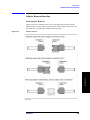
Example of Using Fixture Simulator . . . . . . . . . . . . . . . . . . . . . . . . . . . . . . . . . . . . . . . . . . . . . . . . . . . . .
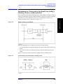
Measurement circuit example for a DUT with balanced port . . . . . . . . . . . . . . . . . . . . . . . . . . . . . . . .
Evaluation using an actual test fixture . . . . . . . . . . . . . . . . . . . . . . . . . . . . . . . . . . . . . . . . . . . . . . . . . .
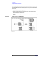
Problems in measurement with an actual test fixture . . . . . . . . . . . . . . . . . . . . . . . . . . . . . . . . . . . . . . .
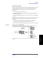
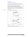
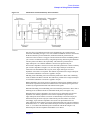
DUT evaluation using the E5070B/E5071B’s fixture simulator . . . . . . . . . . . . . . . . . . . . . . . . . . . . . .
Advantages of balanced DUT evaluation using fixture simulator . . . . . . . . . . . . . . . . . . . . . . . . . . . . .
286
286
287
287
288
288
289
289
292
293
295
297
300
301
301
302
303
303
305
308
308
308
309
310
312
8. Frequency-Offset Measurement (Option 008)
Overview . . . . . . . . . . . . . . . . . . . . . . . . . . . . . . . . . . . . . . . . . . . . . . . . . . . . . . . . . . . . . . . . . . . . . . . . . .
Overview of Frequency-Offset Measurement . . . . . . . . . . . . . . . . . . . . . . . . . . . . . . . . . . . . . . . . . . . .
Measurement of Mixers . . . . . . . . . . . . . . . . . . . . . . . . . . . . . . . . . . . . . . . . . . . . . . . . . . . . . . . . . . . . . . .
Measurement flow . . . . . . . . . . . . . . . . . . . . . . . . . . . . . . . . . . . . . . . . . . . . . . . . . . . . . . . . . . . . . . . . .
1. Setting Frequency-Offset . . . . . . . . . . . . . . . . . . . . . . . . . . . . . . . . . . . . . . . . . . . . . . . . . . . . . . . . . .
2. Setting External Signal Source . . . . . . . . . . . . . . . . . . . . . . . . . . . . . . . . . . . . . . . . . . . . . . . . . . . . . .
3. Avoid Spurious Function . . . . . . . . . . . . . . . . . . . . . . . . . . . . . . . . . . . . . . . . . . . . . . . . . . . . . . . . . .
4. Changing Frequency Data . . . . . . . . . . . . . . . . . . . . . . . . . . . . . . . . . . . . . . . . . . . . . . . . . . . . . . . . .
5. Implementing Mixer Calibration . . . . . . . . . . . . . . . . . . . . . . . . . . . . . . . . . . . . . . . . . . . . . . . . . . . .
6. Conversion Loss Measurement. . . . . . . . . . . . . . . . . . . . . . . . . . . . . . . . . . . . . . . . . . . . . . . . . . . . . .
Measurement of Harmonic Distortion . . . . . . . . . . . . . . . . . . . . . . . . . . . . . . . . . . . . . . . . . . . . . . . . . . . .
Measurement flow . . . . . . . . . . . . . . . . . . . . . . . . . . . . . . . . . . . . . . . . . . . . . . . . . . . . . . . . . . . . . . . . .
1. Setting Frequency-Offset Function. . . . . . . . . . . . . . . . . . . . . . . . . . . . . . . . . . . . . . . . . . . . . . . . . . .
2. Implementing Receiver Calibration . . . . . . . . . . . . . . . . . . . . . . . . . . . . . . . . . . . . . . . . . . . . . . . . . .
3. Setting Absolute Measurement Parameters . . . . . . . . . . . . . . . . . . . . . . . . . . . . . . . . . . . . . . . . . . . .
4. Harmonic Distortion Measurement . . . . . . . . . . . . . . . . . . . . . . . . . . . . . . . . . . . . . . . . . . . . . . . . . .
314
314
315
315
315
318
322
323
325
325
328
328
328
329
329
330
9. Analysis in Time Domain (Option 010)
Overview . . . . . . . . . . . . . . . . . . . . . . . . . . . . . . . . . . . . . . . . . . . . . . . . . . . . . . . . . . . . . . . . . . . . . . . . . . 334
Overview of time domain measurement . . . . . . . . . . . . . . . . . . . . . . . . . . . . . . . . . . . . . . . . . . . . . . . . . 334
Comparison to time domain reflectometry (TDR) measurement . . . . . . . . . . . . . . . . . . . . . . . . . . . . . . 334
14
Contents
Time domain function of E5070B/E5071B. . . . . . . . . . . . . . . . . . . . . . . . . . . . . . . . . . . . . . . . . . . . . . . 335
Transformation to time domain. . . . . . . . . . . . . . . . . . . . . . . . . . . . . . . . . . . . . . . . . . . . . . . . . . . . . . . . . . 336
Measurement flow. . . . . . . . . . . . . . . . . . . . . . . . . . . . . . . . . . . . . . . . . . . . . . . . . . . . . . . . . . . . . . . . . . 336
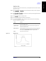
Selecting a type . . . . . . . . . . . . . . . . . . . . . . . . . . . . . . . . . . . . . . . . . . . . . . . . . . . . . . . . . . . . . . . . . . . . 337
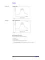
Setting the window . . . . . . . . . . . . . . . . . . . . . . . . . . . . . . . . . . . . . . . . . . . . . . . . . . . . . . . . . . . . . . . . . 339
Calculating necessary measurement conditions . . . . . . . . . . . . . . . . . . . . . . . . . . . . . . . . . . . . . . . . . . . 340
Setting the frequency range and the number of points . . . . . . . . . . . . . . . . . . . . . . . . . . . . . . . . . . . . . . 344
Setting display range . . . . . . . . . . . . . . . . . . . . . . . . . . . . . . . . . . . . . . . . . . . . . . . . . . . . . . . . . . . . . . . . 345
Enabling transformation function . . . . . . . . . . . . . . . . . . . . . . . . . . . . . . . . . . . . . . . . . . . . . . . . . . . . . . 345
Deleting Unnecessary Data in Time Domain (gating) . . . . . . . . . . . . . . . . . . . . . . . . . . . . . . . . . . . . . . . . 347
Measurement Flow . . . . . . . . . . . . . . . . . . . . . . . . . . . . . . . . . . . . . . . . . . . . . . . . . . . . . . . . . . . . . . . . . 347
Setting gate type . . . . . . . . . . . . . . . . . . . . . . . . . . . . . . . . . . . . . . . . . . . . . . . . . . . . . . . . . . . . . . . . . . . 347
Setting gate shape . . . . . . . . . . . . . . . . . . . . . . . . . . . . . . . . . . . . . . . . . . . . . . . . . . . . . . . . . . . . . . . . . . 348
Setting gate range . . . . . . . . . . . . . . . . . . . . . . . . . . . . . . . . . . . . . . . . . . . . . . . . . . . . . . . . . . . . . . . . . . 349
Enabling gating function . . . . . . . . . . . . . . . . . . . . . . . . . . . . . . . . . . . . . . . . . . . . . . . . . . . . . . . . . . . . . 350
Characteristics of Response in Time Domain. . . . . . . . . . . . . . . . . . . . . . . . . . . . . . . . . . . . . . . . . . . . . . . 351
Masking. . . . . . . . . . . . . . . . . . . . . . . . . . . . . . . . . . . . . . . . . . . . . . . . . . . . . . . . . . . . . . . . . . . . . . . . . . 351
Identifying mismatch type. . . . . . . . . . . . . . . . . . . . . . . . . . . . . . . . . . . . . . . . . . . . . . . . . . . . . . . . . . . . 352
10. Data Output
Saving and Recalling Instrument State . . . . . . . . . . . . . . . . . . . . . . . . . . . . . . . . . . . . . . . . . . . . . . . . . . . . 354
Compatibility of files related to saving and recalling . . . . . . . . . . . . . . . . . . . . . . . . . . . . . . . . . . . . . . . 354
Save procedure . . . . . . . . . . . . . . . . . . . . . . . . . . . . . . . . . . . . . . . . . . . . . . . . . . . . . . . . . . . . . . . . . . . . 356
Recall Procedure . . . . . . . . . . . . . . . . . . . . . . . . . . . . . . . . . . . . . . . . . . . . . . . . . . . . . . . . . . . . . . . . . . . 359
Recall Procedure Using “Recall by File Name” Feature . . . . . . . . . . . . . . . . . . . . . . . . . . . . . . . . . . . . 360
Priority of recalling the configuration file at startup. . . . . . . . . . . . . . . . . . . . . . . . . . . . . . . . . . . . . . . . 360
Saving/Recalling Instrument State for Each Channel into/from Memory . . . . . . . . . . . . . . . . . . . . . . . . . 361
Operational Procedure. . . . . . . . . . . . . . . . . . . . . . . . . . . . . . . . . . . . . . . . . . . . . . . . . . . . . . . . . . . . . . . 361
Saving Trace Data to a File. . . . . . . . . . . . . . . . . . . . . . . . . . . . . . . . . . . . . . . . . . . . . . . . . . . . . . . . . . . . . 362
Saving data as a CSV file . . . . . . . . . . . . . . . . . . . . . . . . . . . . . . . . . . . . . . . . . . . . . . . . . . . . . . . . . . . . 362
Saving data in Touchstone format . . . . . . . . . . . . . . . . . . . . . . . . . . . . . . . . . . . . . . . . . . . . . . . . . . . . . . 363
Saving the Screen Image to a File . . . . . . . . . . . . . . . . . . . . . . . . . . . . . . . . . . . . . . . . . . . . . . . . . . . . . . . 368
Saving the Screen Image to a File. . . . . . . . . . . . . . . . . . . . . . . . . . . . . . . . . . . . . . . . . . . . . . . . . . . . . . 368
Organizing Files and Folders . . . . . . . . . . . . . . . . . . . . . . . . . . . . . . . . . . . . . . . . . . . . . . . . . . . . . . . . . . . 369
To Open Windows Explorer . . . . . . . . . . . . . . . . . . . . . . . . . . . . . . . . . . . . . . . . . . . . . . . . . . . . . . . . . . 369
To Copy a File or Folder . . . . . . . . . . . . . . . . . . . . . . . . . . . . . . . . . . . . . . . . . . . . . . . . . . . . . . . . . . . . . 369
To Move a File or Folder. . . . . . . . . . . . . . . . . . . . . . . . . . . . . . . . . . . . . . . . . . . . . . . . . . . . . . . . . . . . . 370
To Delete a File or Folder . . . . . . . . . . . . . . . . . . . . . . . . . . . . . . . . . . . . . . . . . . . . . . . . . . . . . . . . . . . . 370
To Rename a File or Folder. . . . . . . . . . . . . . . . . . . . . . . . . . . . . . . . . . . . . . . . . . . . . . . . . . . . . . . . . . . 370
To Format a Floppy Disk . . . . . . . . . . . . . . . . . . . . . . . . . . . . . . . . . . . . . . . . . . . . . . . . . . . . . . . . . . . . 370
Printing Displayed Screen . . . . . . . . . . . . . . . . . . . . . . . . . . . . . . . . . . . . . . . . . . . . . . . . . . . . . . . . . . . . . 371
Supported printers . . . . . . . . . . . . . . . . . . . . . . . . . . . . . . . . . . . . . . . . . . . . . . . . . . . . . . . . . . . . . . . . . . 371
Printed/saved images. . . . . . . . . . . . . . . . . . . . . . . . . . . . . . . . . . . . . . . . . . . . . . . . . . . . . . . . . . . . . . . . 372
Print Procedure . . . . . . . . . . . . . . . . . . . . . . . . . . . . . . . . . . . . . . . . . . . . . . . . . . . . . . . . . . . . . . . . . . . . 372
11. Limit Test
Limit Test . . . . . . . . . . . . . . . . . . . . . . . . . . . . . . . . . . . . . . . . . . . . . . . . . . . . . . . . . . . . . . . . . . . . . . . . . . 376
Concept of limit test . . . . . . . . . . . . . . . . . . . . . . . . . . . . . . . . . . . . . . . . . . . . . . . . . . . . . . . . . . . . . . . . 376
15
Contents
Displaying judgment result of limit test . . . . . . . . . . . . . . . . . . . . . . . . . . . . . . . . . . . . . . . . . . . . . . . . .
Defining the limit line. . . . . . . . . . . . . . . . . . . . . . . . . . . . . . . . . . . . . . . . . . . . . . . . . . . . . . . . . . . . . . .
Turning the limit test ON/OFF . . . . . . . . . . . . . . . . . . . . . . . . . . . . . . . . . . . . . . . . . . . . . . . . . . . . . . . .
Limit line offset. . . . . . . . . . . . . . . . . . . . . . . . . . . . . . . . . . . . . . . . . . . . . . . . . . . . . . . . . . . . . . . . . . . .
Initializing the limit table . . . . . . . . . . . . . . . . . . . . . . . . . . . . . . . . . . . . . . . . . . . . . . . . . . . . . . . . . . . .
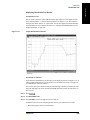
Ripple Test . . . . . . . . . . . . . . . . . . . . . . . . . . . . . . . . . . . . . . . . . . . . . . . . . . . . . . . . . . . . . . . . . . . . . . . . .
Concept of ripple test . . . . . . . . . . . . . . . . . . . . . . . . . . . . . . . . . . . . . . . . . . . . . . . . . . . . . . . . . . . . . . .
Displaying ripple test results. . . . . . . . . . . . . . . . . . . . . . . . . . . . . . . . . . . . . . . . . . . . . . . . . . . . . . . . . .
Configuring ripple limit . . . . . . . . . . . . . . . . . . . . . . . . . . . . . . . . . . . . . . . . . . . . . . . . . . . . . . . . . . . . .
Turning on/off ripple test and displaying results . . . . . . . . . . . . . . . . . . . . . . . . . . . . . . . . . . . . . . . . . .
Initializing the limit table . . . . . . . . . . . . . . . . . . . . . . . . . . . . . . . . . . . . . . . . . . . . . . . . . . . . . . . . . . . .
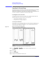
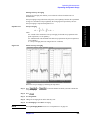
Bandwidth Test . . . . . . . . . . . . . . . . . . . . . . . . . . . . . . . . . . . . . . . . . . . . . . . . . . . . . . . . . . . . . . . . . . . . . .
Displaying Bandwidth Test Results . . . . . . . . . . . . . . . . . . . . . . . . . . . . . . . . . . . . . . . . . . . . . . . . . . . .
Set up bandwidth test . . . . . . . . . . . . . . . . . . . . . . . . . . . . . . . . . . . . . . . . . . . . . . . . . . . . . . . . . . . . . . .
Turning On/Off Bandwidth Test and Displaying Results . . . . . . . . . . . . . . . . . . . . . . . . . . . . . . . . . . . .
377
378
382
383
384
385
385
386
387
390
391
392
393
394
394
12. Optimizing Measurements
Expanding the Dynamic Range . . . . . . . . . . . . . . . . . . . . . . . . . . . . . . . . . . . . . . . . . . . . . . . . . . . . . . . . .
Lowering the receiver noise floor . . . . . . . . . . . . . . . . . . . . . . . . . . . . . . . . . . . . . . . . . . . . . . . . . . . . . .
Reducing Trace Noise . . . . . . . . . . . . . . . . . . . . . . . . . . . . . . . . . . . . . . . . . . . . . . . . . . . . . . . . . . . . . . . .
Turning on Smoothing . . . . . . . . . . . . . . . . . . . . . . . . . . . . . . . . . . . . . . . . . . . . . . . . . . . . . . . . . . . . . .
Improving Phase Measurement Accuracy . . . . . . . . . . . . . . . . . . . . . . . . . . . . . . . . . . . . . . . . . . . . . . . . .
Electrical Delay. . . . . . . . . . . . . . . . . . . . . . . . . . . . . . . . . . . . . . . . . . . . . . . . . . . . . . . . . . . . . . . . . . . .
Phase offset . . . . . . . . . . . . . . . . . . . . . . . . . . . . . . . . . . . . . . . . . . . . . . . . . . . . . . . . . . . . . . . . . . . . . . .
Specifying the velocity factor . . . . . . . . . . . . . . . . . . . . . . . . . . . . . . . . . . . . . . . . . . . . . . . . . . . . . . . . .
Setting Port Extensions and Loss Values . . . . . . . . . . . . . . . . . . . . . . . . . . . . . . . . . . . . . . . . . . . . . . . . . .
Setting port extensions . . . . . . . . . . . . . . . . . . . . . . . . . . . . . . . . . . . . . . . . . . . . . . . . . . . . . . . . . . . . . .
Setting loss values. . . . . . . . . . . . . . . . . . . . . . . . . . . . . . . . . . . . . . . . . . . . . . . . . . . . . . . . . . . . . . . . . .
Enabling port extensions and loss values . . . . . . . . . . . . . . . . . . . . . . . . . . . . . . . . . . . . . . . . . . . . . . . .
Using the auto port extension function . . . . . . . . . . . . . . . . . . . . . . . . . . . . . . . . . . . . . . . . . . . . . . . . . .
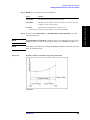
Reducing Measurement Error in High Temperature Environments. . . . . . . . . . . . . . . . . . . . . . . . . . . . . .
Procedure . . . . . . . . . . . . . . . . . . . . . . . . . . . . . . . . . . . . . . . . . . . . . . . . . . . . . . . . . . . . . . . . . . . . . . . .
Improving Measurement Throughput. . . . . . . . . . . . . . . . . . . . . . . . . . . . . . . . . . . . . . . . . . . . . . . . . . . . .
Using Fast Sweep Modes . . . . . . . . . . . . . . . . . . . . . . . . . . . . . . . . . . . . . . . . . . . . . . . . . . . . . . . . . . . .
Turning off the updating of information displayed on the LCD screen . . . . . . . . . . . . . . . . . . . . . . . . .
Turning off system error correction . . . . . . . . . . . . . . . . . . . . . . . . . . . . . . . . . . . . . . . . . . . . . . . . . . . .
Performing a Segment-by-Segment Sweep (segment sweep) . . . . . . . . . . . . . . . . . . . . . . . . . . . . . . . . . .
Concept of Segment Sweep . . . . . . . . . . . . . . . . . . . . . . . . . . . . . . . . . . . . . . . . . . . . . . . . . . . . . . . . . .
Conditions for setting up a segment sweep . . . . . . . . . . . . . . . . . . . . . . . . . . . . . . . . . . . . . . . . . . . . . .
Items that can be set for each segment . . . . . . . . . . . . . . . . . . . . . . . . . . . . . . . . . . . . . . . . . . . . . . . . . .
Sweep delay time and sweep time in a segment sweep . . . . . . . . . . . . . . . . . . . . . . . . . . . . . . . . . . . . .
Frequency base display and order base display . . . . . . . . . . . . . . . . . . . . . . . . . . . . . . . . . . . . . . . . . . .
Procedure . . . . . . . . . . . . . . . . . . . . . . . . . . . . . . . . . . . . . . . . . . . . . . . . . . . . . . . . . . . . . . . . . . . . . . . .
396
396
398
398
400
400
402
402
403
403
404
405
406
411
411
412
412
416
416
417
417
418
418
419
419
421
13. Setting and Using the Control and Management Functions
Setting the GPIB. . . . . . . . . . . . . . . . . . . . . . . . . . . . . . . . . . . . . . . . . . . . . . . . . . . . . . . . . . . . . . . . . . . . . 428
Setting talker/listener GPIB address of E5070B/E5071B . . . . . . . . . . . . . . . . . . . . . . . . . . . . . . . . . . . 428
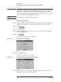
Setting system controller (USB/GPIB interface) when c drive volume label in hard disk is less than CP801
16
Contents
428
Setting system controller (USB/GPIB interface) when c drive volume label in hard disk is more than CP810
431
Setting the Internal Clock . . . . . . . . . . . . . . . . . . . . . . . . . . . . . . . . . . . . . . . . . . . . . . . . . . . . . . . . . . . . . . 433
Setting the Date and Time . . . . . . . . . . . . . . . . . . . . . . . . . . . . . . . . . . . . . . . . . . . . . . . . . . . . . . . . . . . . 433
Setting the Date/Time Display ON/OFF . . . . . . . . . . . . . . . . . . . . . . . . . . . . . . . . . . . . . . . . . . . . . . . . . 434
Setting the Mouse . . . . . . . . . . . . . . . . . . . . . . . . . . . . . . . . . . . . . . . . . . . . . . . . . . . . . . . . . . . . . . . . . . . . 435
Setup Step . . . . . . . . . . . . . . . . . . . . . . . . . . . . . . . . . . . . . . . . . . . . . . . . . . . . . . . . . . . . . . . . . . . . . . . . 435
Configuring the Network . . . . . . . . . . . . . . . . . . . . . . . . . . . . . . . . . . . . . . . . . . . . . . . . . . . . . . . . . . . . . . 438
Enabling/disabling network. . . . . . . . . . . . . . . . . . . . . . . . . . . . . . . . . . . . . . . . . . . . . . . . . . . . . . . . . . . 438
Setting IP address . . . . . . . . . . . . . . . . . . . . . . . . . . . . . . . . . . . . . . . . . . . . . . . . . . . . . . . . . . . . . . . . . . 439
Specifying computer name . . . . . . . . . . . . . . . . . . . . . . . . . . . . . . . . . . . . . . . . . . . . . . . . . . . . . . . . . . . 441
Remote Control Using HTTP . . . . . . . . . . . . . . . . . . . . . . . . . . . . . . . . . . . . . . . . . . . . . . . . . . . . . . . . . . . 443
Required Modification of Settings . . . . . . . . . . . . . . . . . . . . . . . . . . . . . . . . . . . . . . . . . . . . . . . . . . . . . 443
How to Start VNC Server Configuration . . . . . . . . . . . . . . . . . . . . . . . . . . . . . . . . . . . . . . . . . . . . . . . . 443
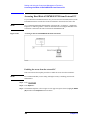
Accessing Hard Disk of E5070B/E5071B from External PC. . . . . . . . . . . . . . . . . . . . . . . . . . . . . . . . . . . 444
Enabling the access form the external PC. . . . . . . . . . . . . . . . . . . . . . . . . . . . . . . . . . . . . . . . . . . . . . . . 444
Accessing hard disk of E5070B/E5071B from external PC . . . . . . . . . . . . . . . . . . . . . . . . . . . . . . . . . . 446
Disabling USB Mass Storage Device . . . . . . . . . . . . . . . . . . . . . . . . . . . . . . . . . . . . . . . . . . . . . . . . . . . . . 447
Steps for Setting Modification . . . . . . . . . . . . . . . . . . . . . . . . . . . . . . . . . . . . . . . . . . . . . . . . . . . . . . . . 447
Locking the Front Keys, Keyboard, and/or Mouse (Touch Screen) . . . . . . . . . . . . . . . . . . . . . . . . . . . . . . 448
Locking the Front Keys, Keyboard, and/or Mouse. . . . . . . . . . . . . . . . . . . . . . . . . . . . . . . . . . . . . . . . . 448
Setting the Beeper (Built-in Speaker) . . . . . . . . . . . . . . . . . . . . . . . . . . . . . . . . . . . . . . . . . . . . . . . . . . . . . 449
Setting the Operation Complete Beeper . . . . . . . . . . . . . . . . . . . . . . . . . . . . . . . . . . . . . . . . . . . . . . . . . 449
Setting the Warning Beeper. . . . . . . . . . . . . . . . . . . . . . . . . . . . . . . . . . . . . . . . . . . . . . . . . . . . . . . . . . . 449
Turning off the LCD Screen Backlight. . . . . . . . . . . . . . . . . . . . . . . . . . . . . . . . . . . . . . . . . . . . . . . . . . . . 450
Turning off the LCD Screen Backlight . . . . . . . . . . . . . . . . . . . . . . . . . . . . . . . . . . . . . . . . . . . . . . . . . . 450
Checking the product information . . . . . . . . . . . . . . . . . . . . . . . . . . . . . . . . . . . . . . . . . . . . . . . . . . . . . . . 451
Checking the serial number. . . . . . . . . . . . . . . . . . . . . . . . . . . . . . . . . . . . . . . . . . . . . . . . . . . . . . . . . . . 451
Checking other product information . . . . . . . . . . . . . . . . . . . . . . . . . . . . . . . . . . . . . . . . . . . . . . . . . . . . 451
Setting the preset function . . . . . . . . . . . . . . . . . . . . . . . . . . . . . . . . . . . . . . . . . . . . . . . . . . . . . . . . . . . . . 453
Showing/hiding the confirmation buttons when presetting. . . . . . . . . . . . . . . . . . . . . . . . . . . . . . . . . . . 453
Setting the user preset function . . . . . . . . . . . . . . . . . . . . . . . . . . . . . . . . . . . . . . . . . . . . . . . . . . . . . . . . 453
Saving a user-preset instrument state . . . . . . . . . . . . . . . . . . . . . . . . . . . . . . . . . . . . . . . . . . . . . . . . . . . 454
System Recovery . . . . . . . . . . . . . . . . . . . . . . . . . . . . . . . . . . . . . . . . . . . . . . . . . . . . . . . . . . . . . . . . . . . . 455
Types of system recoveries . . . . . . . . . . . . . . . . . . . . . . . . . . . . . . . . . . . . . . . . . . . . . . . . . . . . . . . . . . . 455
Notes on executing system recovery . . . . . . . . . . . . . . . . . . . . . . . . . . . . . . . . . . . . . . . . . . . . . . . . . . . 455
Procedure to execute the factory function (1) . . . . . . . . . . . . . . . . . . . . . . . . . . . . . . . . . . . . . . . . . . . . . 456
Procedure to create the user backup image (1) . . . . . . . . . . . . . . . . . . . . . . . . . . . . . . . . . . . . . . . . . . . . 459
Procedure to execute the user recovery function (1). . . . . . . . . . . . . . . . . . . . . . . . . . . . . . . . . . . . . . . . 462
Procedure to execute the factory recovery function (2) . . . . . . . . . . . . . . . . . . . . . . . . . . . . . . . . . . . . . 465
Procedure to create the user backup image (2) . . . . . . . . . . . . . . . . . . . . . . . . . . . . . . . . . . . . . . . . . . . . 468
Procedure to execute the user recovery function (2). . . . . . . . . . . . . . . . . . . . . . . . . . . . . . . . . . . . . . . . 471
Calibration of the Touch Screen . . . . . . . . . . . . . . . . . . . . . . . . . . . . . . . . . . . . . . . . . . . . . . . . . . . . . . . . . 474
Initial Source Port Control function . . . . . . . . . . . . . . . . . . . . . . . . . . . . . . . . . . . . . . . . . . . . . . . . . . . . . . 475
14. Controlling E5091A
Connecting E5070B/E5071B and E5091A. . . . . . . . . . . . . . . . . . . . . . . . . . . . . . . . . . . . . . . . . . . . . . . . . 478
Required devices . . . . . . . . . . . . . . . . . . . . . . . . . . . . . . . . . . . . . . . . . . . . . . . . . . . . . . . . . . . . . . . . . . . 478
17
Contents
Connecting E5070B/E5071B and E5091A. . . . . . . . . . . . . . . . . . . . . . . . . . . . . . . . . . . . . . . . . . . . . . .
Powering on . . . . . . . . . . . . . . . . . . . . . . . . . . . . . . . . . . . . . . . . . . . . . . . . . . . . . . . . . . . . . . . . . . . . . .
Setting the E5091A. . . . . . . . . . . . . . . . . . . . . . . . . . . . . . . . . . . . . . . . . . . . . . . . . . . . . . . . . . . . . . . . . . .
Selecting ID for E5091A . . . . . . . . . . . . . . . . . . . . . . . . . . . . . . . . . . . . . . . . . . . . . . . . . . . . . . . . . . . .
Selecting the E5091A Model . . . . . . . . . . . . . . . . . . . . . . . . . . . . . . . . . . . . . . . . . . . . . . . . . . . . . . . . .
Assigning test ports. . . . . . . . . . . . . . . . . . . . . . . . . . . . . . . . . . . . . . . . . . . . . . . . . . . . . . . . . . . . . . . . .
Displaying the E5091A properties . . . . . . . . . . . . . . . . . . . . . . . . . . . . . . . . . . . . . . . . . . . . . . . . . . . . .
Setting control line . . . . . . . . . . . . . . . . . . . . . . . . . . . . . . . . . . . . . . . . . . . . . . . . . . . . . . . . . . . . . . . . .
Enabling control of E5091A . . . . . . . . . . . . . . . . . . . . . . . . . . . . . . . . . . . . . . . . . . . . . . . . . . . . . . . . . .
Calibration . . . . . . . . . . . . . . . . . . . . . . . . . . . . . . . . . . . . . . . . . . . . . . . . . . . . . . . . . . . . . . . . . . . . . . . . .
Performing Measurement . . . . . . . . . . . . . . . . . . . . . . . . . . . . . . . . . . . . . . . . . . . . . . . . . . . . . . . . . . . . . .
Trigger state and switching the setting of the E5091A. . . . . . . . . . . . . . . . . . . . . . . . . . . . . . . . . . . . . .
Operation . . . . . . . . . . . . . . . . . . . . . . . . . . . . . . . . . . . . . . . . . . . . . . . . . . . . . . . . . . . . . . . . . . . . . . . .
Connecting Two E5091As . . . . . . . . . . . . . . . . . . . . . . . . . . . . . . . . . . . . . . . . . . . . . . . . . . . . . . . . . . . . .
478
479
480
480
481
481
483
484
485
486
487
487
487
488
15. Measurement Examples
Measuring the SAW Bandpass Filter Using the Segment Sweep . . . . . . . . . . . . . . . . . . . . . . . . . . . . . . .
Evaluation Steps . . . . . . . . . . . . . . . . . . . . . . . . . . . . . . . . . . . . . . . . . . . . . . . . . . . . . . . . . . . . . . . . . . .
1. Determine the Segment Sweep Conditions . . . . . . . . . . . . . . . . . . . . . . . . . . . . . . . . . . . . . . . . . . . .
2. Create a Segment Sweep Table. . . . . . . . . . . . . . . . . . . . . . . . . . . . . . . . . . . . . . . . . . . . . . . . . . . . . .
3. Select the Segment Sweep as the Sweep Type . . . . . . . . . . . . . . . . . . . . . . . . . . . . . . . . . . . . . . . . . .
4. Execute the Calibration. . . . . . . . . . . . . . . . . . . . . . . . . . . . . . . . . . . . . . . . . . . . . . . . . . . . . . . . . . . .
5. Connect the DUT . . . . . . . . . . . . . . . . . . . . . . . . . . . . . . . . . . . . . . . . . . . . . . . . . . . . . . . . . . . . . . . .
6. Execute the Measurement . . . . . . . . . . . . . . . . . . . . . . . . . . . . . . . . . . . . . . . . . . . . . . . . . . . . . . . . . .
7. Define the Setup for Display . . . . . . . . . . . . . . . . . . . . . . . . . . . . . . . . . . . . . . . . . . . . . . . . . . . . . . .
Evaluating a Duplexer . . . . . . . . . . . . . . . . . . . . . . . . . . . . . . . . . . . . . . . . . . . . . . . . . . . . . . . . . . . . . . . .
Evaluation Steps . . . . . . . . . . . . . . . . . . . . . . . . . . . . . . . . . . . . . . . . . . . . . . . . . . . . . . . . . . . . . . . . . . .
1. Determine the Segment Sweep Conditions . . . . . . . . . . . . . . . . . . . . . . . . . . . . . . . . . . . . . . . . . . . .
2. Create a Segment Sweep Table. . . . . . . . . . . . . . . . . . . . . . . . . . . . . . . . . . . . . . . . . . . . . . . . . . . . . .
3. Select the Segment Sweep as the Sweep Type . . . . . . . . . . . . . . . . . . . . . . . . . . . . . . . . . . . . . . . . . .
4. Execute the Calibration. . . . . . . . . . . . . . . . . . . . . . . . . . . . . . . . . . . . . . . . . . . . . . . . . . . . . . . . . . . .
5. Connect the DUT . . . . . . . . . . . . . . . . . . . . . . . . . . . . . . . . . . . . . . . . . . . . . . . . . . . . . . . . . . . . . . . .
6. Define the Setup for Display . . . . . . . . . . . . . . . . . . . . . . . . . . . . . . . . . . . . . . . . . . . . . . . . . . . . . . .
7. Execute the Measurement . . . . . . . . . . . . . . . . . . . . . . . . . . . . . . . . . . . . . . . . . . . . . . . . . . . . . . . . . .
8. Define the Setup for the Segment Display and Scale . . . . . . . . . . . . . . . . . . . . . . . . . . . . . . . . . . . . .
9. Analyze the Parameters . . . . . . . . . . . . . . . . . . . . . . . . . . . . . . . . . . . . . . . . . . . . . . . . . . . . . . . . . . .
10. Define the Setup for a Limit Table . . . . . . . . . . . . . . . . . . . . . . . . . . . . . . . . . . . . . . . . . . . . . . . . . .
11. Execute the Limit Test . . . . . . . . . . . . . . . . . . . . . . . . . . . . . . . . . . . . . . . . . . . . . . . . . . . . . . . . . . .
Measuring the Deviation from a Linear Phase . . . . . . . . . . . . . . . . . . . . . . . . . . . . . . . . . . . . . . . . . . . . . .
Evaluation Steps . . . . . . . . . . . . . . . . . . . . . . . . . . . . . . . . . . . . . . . . . . . . . . . . . . . . . . . . . . . . . . . . . . .
1. Connect the DUT . . . . . . . . . . . . . . . . . . . . . . . . . . . . . . . . . . . . . . . . . . . . . . . . . . . . . . . . . . . . . . . .
2. Define the Measurement Conditions . . . . . . . . . . . . . . . . . . . . . . . . . . . . . . . . . . . . . . . . . . . . . . . . .
3. Execute the Calibration. . . . . . . . . . . . . . . . . . . . . . . . . . . . . . . . . . . . . . . . . . . . . . . . . . . . . . . . . . . .
4. Connect the DUT and Execute the Auto Scale. . . . . . . . . . . . . . . . . . . . . . . . . . . . . . . . . . . . . . . . . .
5. Specify the Electrical Delay . . . . . . . . . . . . . . . . . . . . . . . . . . . . . . . . . . . . . . . . . . . . . . . . . . . . . . . .
6. Measure the Deviation from a Linear Phase. . . . . . . . . . . . . . . . . . . . . . . . . . . . . . . . . . . . . . . . . . . .
Measuring an Unbalanced and Balanced Bandpass Filter . . . . . . . . . . . . . . . . . . . . . . . . . . . . . . . . . . . . .
Evaluation Steps . . . . . . . . . . . . . . . . . . . . . . . . . . . . . . . . . . . . . . . . . . . . . . . . . . . . . . . . . . . . . . . . . . .
1. Connecting the DUT . . . . . . . . . . . . . . . . . . . . . . . . . . . . . . . . . . . . . . . . . . . . . . . . . . . . . . . . . . . . . .
490
490
491
492
494
494
495
495
495
497
497
497
498
499
499
501
502
502
502
503
505
506
509
509
509
510
510
510
511
512
513
513
514
18
Contents
2. Setting the Measurement Conditions . . . . . . . . . . . . . . . . . . . . . . . . . . . . . . . . . . . . . . . . . . . . . . . . . 515
3. Performing Calibration . . . . . . . . . . . . . . . . . . . . . . . . . . . . . . . . . . . . . . . . . . . . . . . . . . . . . . . . . . . . 516
4. Setting a Balance Conversion Topology . . . . . . . . . . . . . . . . . . . . . . . . . . . . . . . . . . . . . . . . . . . . . . . 517
5. Selecting Measurement Parameters . . . . . . . . . . . . . . . . . . . . . . . . . . . . . . . . . . . . . . . . . . . . . . . . . . 517
6. Extending the Calibration Plane (removing the cause of error) . . . . . . . . . . . . . . . . . . . . . . . . . . . . . 519
7. Setting the Port Reference Impedances. . . . . . . . . . . . . . . . . . . . . . . . . . . . . . . . . . . . . . . . . . . . . . . . 519
8. Adding a Matching Circuit . . . . . . . . . . . . . . . . . . . . . . . . . . . . . . . . . . . . . . . . . . . . . . . . . . . . . . . . . 521
Measuring Parameters with Cable . . . . . . . . . . . . . . . . . . . . . . . . . . . . . . . . . . . . . . . . . . . . . . . . . . . . . . . 522
Overview of evaluation procedure . . . . . . . . . . . . . . . . . . . . . . . . . . . . . . . . . . . . . . . . . . . . . . . . . . . . . 522
1. Setting the Measurement Conditions . . . . . . . . . . . . . . . . . . . . . . . . . . . . . . . . . . . . . . . . . . . . . . . . . 522
2. Executing Calibration . . . . . . . . . . . . . . . . . . . . . . . . . . . . . . . . . . . . . . . . . . . . . . . . . . . . . . . . . . . . . 522
3. Connecting the DUT . . . . . . . . . . . . . . . . . . . . . . . . . . . . . . . . . . . . . . . . . . . . . . . . . . . . . . . . . . . . . . 523
4. Auto Scale . . . . . . . . . . . . . . . . . . . . . . . . . . . . . . . . . . . . . . . . . . . . . . . . . . . . . . . . . . . . . . . . . . . . . . 523
5. Setting the Time Domain Function . . . . . . . . . . . . . . . . . . . . . . . . . . . . . . . . . . . . . . . . . . . . . . . . . . . 524
Evaluating Transmission Characteristics of a Front End Module . . . . . . . . . . . . . . . . . . . . . . . . . . . . . . . 525
Overview of evaluation procedure . . . . . . . . . . . . . . . . . . . . . . . . . . . . . . . . . . . . . . . . . . . . . . . . . . . . . 525
1. Determining Measurement Conditions . . . . . . . . . . . . . . . . . . . . . . . . . . . . . . . . . . . . . . . . . . . . . . . . 526
2. Setting Channel Window Allocation. . . . . . . . . . . . . . . . . . . . . . . . . . . . . . . . . . . . . . . . . . . . . . . . . . 526
3. Setting the Test Ports. . . . . . . . . . . . . . . . . . . . . . . . . . . . . . . . . . . . . . . . . . . . . . . . . . . . . . . . . . . . . . 526
4. Setting Control Line . . . . . . . . . . . . . . . . . . . . . . . . . . . . . . . . . . . . . . . . . . . . . . . . . . . . . . . . . . . . . . 527
5. Setting Sweep Conditions . . . . . . . . . . . . . . . . . . . . . . . . . . . . . . . . . . . . . . . . . . . . . . . . . . . . . . . . . . 527
6. Setting Balance Conversion Topology . . . . . . . . . . . . . . . . . . . . . . . . . . . . . . . . . . . . . . . . . . . . . . . . 527
7. Selecting Measurement Parameter . . . . . . . . . . . . . . . . . . . . . . . . . . . . . . . . . . . . . . . . . . . . . . . . . . . 528
8. Executing Calibration . . . . . . . . . . . . . . . . . . . . . . . . . . . . . . . . . . . . . . . . . . . . . . . . . . . . . . . . . . . . . 528
9. Connecting DUT . . . . . . . . . . . . . . . . . . . . . . . . . . . . . . . . . . . . . . . . . . . . . . . . . . . . . . . . . . . . . . . . . 530
10. Executing Measurement . . . . . . . . . . . . . . . . . . . . . . . . . . . . . . . . . . . . . . . . . . . . . . . . . . . . . . . . . . 531
Executing Power Calibration . . . . . . . . . . . . . . . . . . . . . . . . . . . . . . . . . . . . . . . . . . . . . . . . . . . . . . . . . . . 533
Overview of execution procedure . . . . . . . . . . . . . . . . . . . . . . . . . . . . . . . . . . . . . . . . . . . . . . . . . . . . . . 533
1. Connecting Power Meter. . . . . . . . . . . . . . . . . . . . . . . . . . . . . . . . . . . . . . . . . . . . . . . . . . . . . . . . . . . 533
2. Setting Address of Power Meter . . . . . . . . . . . . . . . . . . . . . . . . . . . . . . . . . . . . . . . . . . . . . . . . . . . . . 534
3. Setting Stimulus Condition . . . . . . . . . . . . . . . . . . . . . . . . . . . . . . . . . . . . . . . . . . . . . . . . . . . . . . . . . 534
4. Executing Zero Adjustment and Calibration of Power Sensor . . . . . . . . . . . . . . . . . . . . . . . . . . . . . . 534
5. Setting Calibration Data Measurement Conditions. . . . . . . . . . . . . . . . . . . . . . . . . . . . . . . . . . . . . . . 534
6. Connecting Power Sensor . . . . . . . . . . . . . . . . . . . . . . . . . . . . . . . . . . . . . . . . . . . . . . . . . . . . . . . . . . 535
7. Measuring Calibration Data . . . . . . . . . . . . . . . . . . . . . . . . . . . . . . . . . . . . . . . . . . . . . . . . . . . . . . . . 535
16. Specifications and Supplemental Information
Definitions . . . . . . . . . . . . . . . . . . . . . . . . . . . . . . . . . . . . . . . . . . . . . . . . . . . . . . . . . . . . . . . . . . . . . . . . . 538
Corrected System Performance . . . . . . . . . . . . . . . . . . . . . . . . . . . . . . . . . . . . . . . . . . . . . . . . . . . . . . . . . 539
Uncorrected System Performance . . . . . . . . . . . . . . . . . . . . . . . . . . . . . . . . . . . . . . . . . . . . . . . . . . . . . . . 544
Test Port Output (Source) . . . . . . . . . . . . . . . . . . . . . . . . . . . . . . . . . . . . . . . . . . . . . . . . . . . . . . . . . . . . . . 545
Test Port Input. . . . . . . . . . . . . . . . . . . . . . . . . . . . . . . . . . . . . . . . . . . . . . . . . . . . . . . . . . . . . . . . . . . . . . . 547
General Information . . . . . . . . . . . . . . . . . . . . . . . . . . . . . . . . . . . . . . . . . . . . . . . . . . . . . . . . . . . . . . . . . . 551
Measurement Throughput Summary . . . . . . . . . . . . . . . . . . . . . . . . . . . . . . . . . . . . . . . . . . . . . . . . . . . . . 559
Measurement capabilities . . . . . . . . . . . . . . . . . . . . . . . . . . . . . . . . . . . . . . . . . . . . . . . . . . . . . . . . . . . . . . 562
Source control . . . . . . . . . . . . . . . . . . . . . . . . . . . . . . . . . . . . . . . . . . . . . . . . . . . . . . . . . . . . . . . . . . . . . . . 563
Trace functions . . . . . . . . . . . . . . . . . . . . . . . . . . . . . . . . . . . . . . . . . . . . . . . . . . . . . . . . . . . . . . . . . . . . . . 563
Data accuracy enhancement . . . . . . . . . . . . . . . . . . . . . . . . . . . . . . . . . . . . . . . . . . . . . . . . . . . . . . . . . . . . 564
Storage . . . . . . . . . . . . . . . . . . . . . . . . . . . . . . . . . . . . . . . . . . . . . . . . . . . . . . . . . . . . . . . . . . . . . . . . . . . . 565
19
Contents
System capabilities . . . . . . . . . . . . . . . . . . . . . . . . . . . . . . . . . . . . . . . . . . . . . . . . . . . . . . . . . . . . . . . . . . . 565
Automation . . . . . . . . . . . . . . . . . . . . . . . . . . . . . . . . . . . . . . . . . . . . . . . . . . . . . . . . . . . . . . . . . . . . . . . . . 566
17. Measurement Accessories
Test Port Cables . . . . . . . . . . . . . . . . . . . . . . . . . . . . . . . . . . . . . . . . . . . . . . . . . . . . . . . . . . . . . . . . . . . . .
N6314A 50 Ω N Type RF Cable (300 kHz ~ 9 GHz). . . . . . . . . . . . . . . . . . . . . . . . . . . . . . . . . . . . . . .
N6315A 50 Ω N Type RF Cable (300 kHz ~ 9 GHz). . . . . . . . . . . . . . . . . . . . . . . . . . . . . . . . . . . . . . .
Calibration Kits . . . . . . . . . . . . . . . . . . . . . . . . . . . . . . . . . . . . . . . . . . . . . . . . . . . . . . . . . . . . . . . . . . . . .
For Devices with N Type Connectors. . . . . . . . . . . . . . . . . . . . . . . . . . . . . . . . . . . . . . . . . . . . . . . . . . .
For Devices with 3.5 mm (SMA) Connectors . . . . . . . . . . . . . . . . . . . . . . . . . . . . . . . . . . . . . . . . . . . .
For Devices with 7 mm Connectors . . . . . . . . . . . . . . . . . . . . . . . . . . . . . . . . . . . . . . . . . . . . . . . . . . . .
For Devices with 7-16 Connectors . . . . . . . . . . . . . . . . . . . . . . . . . . . . . . . . . . . . . . . . . . . . . . . . . . . . .
Adaptors . . . . . . . . . . . . . . . . . . . . . . . . . . . . . . . . . . . . . . . . . . . . . . . . . . . . . . . . . . . . . . . . . . . . . . . . . . .
11853A 50 Ω N Type Accessory Kit . . . . . . . . . . . . . . . . . . . . . . . . . . . . . . . . . . . . . . . . . . . . . . . . . . .
11878A N type to 3.5 mm Adaptor Kit . . . . . . . . . . . . . . . . . . . . . . . . . . . . . . . . . . . . . . . . . . . . . . . . .
11854A 50 Ω BNC Accessory Kit . . . . . . . . . . . . . . . . . . . . . . . . . . . . . . . . . . . . . . . . . . . . . . . . . . . . .
11852B Minimum-loss pad. . . . . . . . . . . . . . . . . . . . . . . . . . . . . . . . . . . . . . . . . . . . . . . . . . . . . . . . . . .
System Accessories . . . . . . . . . . . . . . . . . . . . . . . . . . . . . . . . . . . . . . . . . . . . . . . . . . . . . . . . . . . . . . . . . .
System Racks and Cases. . . . . . . . . . . . . . . . . . . . . . . . . . . . . . . . . . . . . . . . . . . . . . . . . . . . . . . . . . . . .
GP-IB Cables . . . . . . . . . . . . . . . . . . . . . . . . . . . . . . . . . . . . . . . . . . . . . . . . . . . . . . . . . . . . . . . . . . . . .
82357A/B USB/GPIB Interface . . . . . . . . . . . . . . . . . . . . . . . . . . . . . . . . . . . . . . . . . . . . . . . . . . . . . . .
568
568
568
569
569
572
575
576
577
577
577
577
577
578
578
578
578
18. Information on Maintenance
Backing Up the Data . . . . . . . . . . . . . . . . . . . . . . . . . . . . . . . . . . . . . . . . . . . . . . . . . . . . . . . . . . . . . . . . .
Making Backup Files . . . . . . . . . . . . . . . . . . . . . . . . . . . . . . . . . . . . . . . . . . . . . . . . . . . . . . . . . . . . . . .
Removing/Mounting Removable Hard Disk . . . . . . . . . . . . . . . . . . . . . . . . . . . . . . . . . . . . . . . . . . . . . . .
Removing Removable Hard Disk . . . . . . . . . . . . . . . . . . . . . . . . . . . . . . . . . . . . . . . . . . . . . . . . . . . . . .
Mounting Removable Hard Disk . . . . . . . . . . . . . . . . . . . . . . . . . . . . . . . . . . . . . . . . . . . . . . . . . . . . . .
Writing System Correction Data from Backup Memory to Removable Hard Disk . . . . . . . . . . . . . . . .
Cleaning this Instrument. . . . . . . . . . . . . . . . . . . . . . . . . . . . . . . . . . . . . . . . . . . . . . . . . . . . . . . . . . . . . . .
Cleaning an LCD . . . . . . . . . . . . . . . . . . . . . . . . . . . . . . . . . . . . . . . . . . . . . . . . . . . . . . . . . . . . . . . . . .
Maintenance of Test Ports and Other Connectors/Ports . . . . . . . . . . . . . . . . . . . . . . . . . . . . . . . . . . . . .
Cleaning a Display Other than an LCD . . . . . . . . . . . . . . . . . . . . . . . . . . . . . . . . . . . . . . . . . . . . . . . . .
Replacement of Parts with Limited Service Life . . . . . . . . . . . . . . . . . . . . . . . . . . . . . . . . . . . . . . . . . . . .
Cautions Applicable to Requesting Repair, Replacement, Regular Calibration, etc. . . . . . . . . . . . . . . . .
Backing Up Data in the Hard Disk . . . . . . . . . . . . . . . . . . . . . . . . . . . . . . . . . . . . . . . . . . . . . . . . . . . . .
Devices to be Sent Back for Repair or Regular Calibration . . . . . . . . . . . . . . . . . . . . . . . . . . . . . . . . . .
Recommended Calibration Period . . . . . . . . . . . . . . . . . . . . . . . . . . . . . . . . . . . . . . . . . . . . . . . . . . . . .
580
580
581
581
581
583
584
584
584
584
585
586
586
586
586
A. Manual Changes
Manual Changes . . . . . . . . . . . . . . . . . . . . . . . . . . . . . . . . . . . . . . . . . . . . . . . . . . . . . . . . . . . . . . . . . . . . .
Change 15 . . . . . . . . . . . . . . . . . . . . . . . . . . . . . . . . . . . . . . . . . . . . . . . . . . . . . . . . . . . . . . . . . . . . . . . .
Change 14 . . . . . . . . . . . . . . . . . . . . . . . . . . . . . . . . . . . . . . . . . . . . . . . . . . . . . . . . . . . . . . . . . . . . . . . .
Change 13 . . . . . . . . . . . . . . . . . . . . . . . . . . . . . . . . . . . . . . . . . . . . . . . . . . . . . . . . . . . . . . . . . . . . . . . .
Change 12 . . . . . . . . . . . . . . . . . . . . . . . . . . . . . . . . . . . . . . . . . . . . . . . . . . . . . . . . . . . . . . . . . . . . . . . .
Change11 . . . . . . . . . . . . . . . . . . . . . . . . . . . . . . . . . . . . . . . . . . . . . . . . . . . . . . . . . . . . . . . . . . . . . . . .
Change 10 . . . . . . . . . . . . . . . . . . . . . . . . . . . . . . . . . . . . . . . . . . . . . . . . . . . . . . . . . . . . . . . . . . . . . . . .
Change 9 . . . . . . . . . . . . . . . . . . . . . . . . . . . . . . . . . . . . . . . . . . . . . . . . . . . . . . . . . . . . . . . . . . . . . . . . .
588
589
589
589
589
599
603
604
20
Contents
Change 8 . . . . . . . . . . . . . . . . . . . . . . . . . . . . . . . . . . . . . . . . . . . . . . . . . . . . . . . . . . . . . . . . . . . . . . . . . 605
Change 7 . . . . . . . . . . . . . . . . . . . . . . . . . . . . . . . . . . . . . . . . . . . . . . . . . . . . . . . . . . . . . . . . . . . . . . . . . 605
Change 6 . . . . . . . . . . . . . . . . . . . . . . . . . . . . . . . . . . . . . . . . . . . . . . . . . . . . . . . . . . . . . . . . . . . . . . . . . 606
Change 5 . . . . . . . . . . . . . . . . . . . . . . . . . . . . . . . . . . . . . . . . . . . . . . . . . . . . . . . . . . . . . . . . . . . . . . . . . 606
Change 4 . . . . . . . . . . . . . . . . . . . . . . . . . . . . . . . . . . . . . . . . . . . . . . . . . . . . . . . . . . . . . . . . . . . . . . . . . 609
Change 3 . . . . . . . . . . . . . . . . . . . . . . . . . . . . . . . . . . . . . . . . . . . . . . . . . . . . . . . . . . . . . . . . . . . . . . . . . 609
Change 2 . . . . . . . . . . . . . . . . . . . . . . . . . . . . . . . . . . . . . . . . . . . . . . . . . . . . . . . . . . . . . . . . . . . . . . . . . 609
Change 1 . . . . . . . . . . . . . . . . . . . . . . . . . . . . . . . . . . . . . . . . . . . . . . . . . . . . . . . . . . . . . . . . . . . . . . . . . 609
B. Troubleshooting
Troubleshooting . . . . . . . . . . . . . . . . . . . . . . . . . . . . . . . . . . . . . . . . . . . . . . . . . . . . . . . . . . . . . . . . . . . . . 612
Troubleshooting during Startup. . . . . . . . . . . . . . . . . . . . . . . . . . . . . . . . . . . . . . . . . . . . . . . . . . . . . . . . 612
Troubleshooting during Operation . . . . . . . . . . . . . . . . . . . . . . . . . . . . . . . . . . . . . . . . . . . . . . . . . . . . . 613
Troubleshooting for External Devices . . . . . . . . . . . . . . . . . . . . . . . . . . . . . . . . . . . . . . . . . . . . . . . . . . 616
Error Messages . . . . . . . . . . . . . . . . . . . . . . . . . . . . . . . . . . . . . . . . . . . . . . . . . . . . . . . . . . . . . . . . . . . . . . 617
A . . . . . . . . . . . . . . . . . . . . . . . . . . . . . . . . . . . . . . . . . . . . . . . . . . . . . . . . . . . . . . . . . . . . . . . . . . . . . . . 617
B . . . . . . . . . . . . . . . . . . . . . . . . . . . . . . . . . . . . . . . . . . . . . . . . . . . . . . . . . . . . . . . . . . . . . . . . . . . . . . . 617
C . . . . . . . . . . . . . . . . . . . . . . . . . . . . . . . . . . . . . . . . . . . . . . . . . . . . . . . . . . . . . . . . . . . . . . . . . . . . . . . 617
D . . . . . . . . . . . . . . . . . . . . . . . . . . . . . . . . . . . . . . . . . . . . . . . . . . . . . . . . . . . . . . . . . . . . . . . . . . . . . . . 618
E . . . . . . . . . . . . . . . . . . . . . . . . . . . . . . . . . . . . . . . . . . . . . . . . . . . . . . . . . . . . . . . . . . . . . . . . . . . . . . . 618
F. . . . . . . . . . . . . . . . . . . . . . . . . . . . . . . . . . . . . . . . . . . . . . . . . . . . . . . . . . . . . . . . . . . . . . . . . . . . . . . . 619
G . . . . . . . . . . . . . . . . . . . . . . . . . . . . . . . . . . . . . . . . . . . . . . . . . . . . . . . . . . . . . . . . . . . . . . . . . . . . . . . 620
H . . . . . . . . . . . . . . . . . . . . . . . . . . . . . . . . . . . . . . . . . . . . . . . . . . . . . . . . . . . . . . . . . . . . . . . . . . . . . . . 620
I . . . . . . . . . . . . . . . . . . . . . . . . . . . . . . . . . . . . . . . . . . . . . . . . . . . . . . . . . . . . . . . . . . . . . . . . . . . . . . . . 620
L . . . . . . . . . . . . . . . . . . . . . . . . . . . . . . . . . . . . . . . . . . . . . . . . . . . . . . . . . . . . . . . . . . . . . . . . . . . . . . . 622
M . . . . . . . . . . . . . . . . . . . . . . . . . . . . . . . . . . . . . . . . . . . . . . . . . . . . . . . . . . . . . . . . . . . . . . . . . . . . . . . 622
N . . . . . . . . . . . . . . . . . . . . . . . . . . . . . . . . . . . . . . . . . . . . . . . . . . . . . . . . . . . . . . . . . . . . . . . . . . . . . . . 622
O . . . . . . . . . . . . . . . . . . . . . . . . . . . . . . . . . . . . . . . . . . . . . . . . . . . . . . . . . . . . . . . . . . . . . . . . . . . . . . . 623
P. . . . . . . . . . . . . . . . . . . . . . . . . . . . . . . . . . . . . . . . . . . . . . . . . . . . . . . . . . . . . . . . . . . . . . . . . . . . . . . . 623
Q . . . . . . . . . . . . . . . . . . . . . . . . . . . . . . . . . . . . . . . . . . . . . . . . . . . . . . . . . . . . . . . . . . . . . . . . . . . . . . . 625
R . . . . . . . . . . . . . . . . . . . . . . . . . . . . . . . . . . . . . . . . . . . . . . . . . . . . . . . . . . . . . . . . . . . . . . . . . . . . . . . 625
S. . . . . . . . . . . . . . . . . . . . . . . . . . . . . . . . . . . . . . . . . . . . . . . . . . . . . . . . . . . . . . . . . . . . . . . . . . . . . . . . 626
T . . . . . . . . . . . . . . . . . . . . . . . . . . . . . . . . . . . . . . . . . . . . . . . . . . . . . . . . . . . . . . . . . . . . . . . . . . . . . . . 627
U . . . . . . . . . . . . . . . . . . . . . . . . . . . . . . . . . . . . . . . . . . . . . . . . . . . . . . . . . . . . . . . . . . . . . . . . . . . . . . . 628
V . . . . . . . . . . . . . . . . . . . . . . . . . . . . . . . . . . . . . . . . . . . . . . . . . . . . . . . . . . . . . . . . . . . . . . . . . . . . . . . 628
Warning Message . . . . . . . . . . . . . . . . . . . . . . . . . . . . . . . . . . . . . . . . . . . . . . . . . . . . . . . . . . . . . . . . . . . . 630
C. List of Default Values
List of Default Values, Save/Recall Settings, and Backup Settings . . . . . . . . . . . . . . . . . . . . . . . . . . . . . . 634
D. Softkey Functions
E5070B/E5071B Menu (Top Menu). . . . . . . . . . . . . . . . . . . . . . . . . . . . . . . . . . . . . . . . . . . . . . . . . . . . . . 650
Analysis Menu . . . . . . . . . . . . . . . . . . . . . . . . . . . . . . . . . . . . . . . . . . . . . . . . . . . . . . . . . . . . . . . . . . . . . . 651
Average Menu . . . . . . . . . . . . . . . . . . . . . . . . . . . . . . . . . . . . . . . . . . . . . . . . . . . . . . . . . . . . . . . . . . . . . . . 666
Calibration Menu . . . . . . . . . . . . . . . . . . . . . . . . . . . . . . . . . . . . . . . . . . . . . . . . . . . . . . . . . . . . . . . . . . . . 667
Display Menu . . . . . . . . . . . . . . . . . . . . . . . . . . . . . . . . . . . . . . . . . . . . . . . . . . . . . . . . . . . . . . . . . . . . . . . 694
Format Menu. . . . . . . . . . . . . . . . . . . . . . . . . . . . . . . . . . . . . . . . . . . . . . . . . . . . . . . . . . . . . . . . . . . . . . . . 698
Macro Setup Menu . . . . . . . . . . . . . . . . . . . . . . . . . . . . . . . . . . . . . . . . . . . . . . . . . . . . . . . . . . . . . . . . . . . 699
21
Contents
Marker Menu . . . . . . . . . . . . . . . . . . . . . . . . . . . . . . . . . . . . . . . . . . . . . . . . . . . . . . . . . . . . . . . . . . . . . . .
Marker Function Menu. . . . . . . . . . . . . . . . . . . . . . . . . . . . . . . . . . . . . . . . . . . . . . . . . . . . . . . . . . . . . . . .
Marker Search Menu . . . . . . . . . . . . . . . . . . . . . . . . . . . . . . . . . . . . . . . . . . . . . . . . . . . . . . . . . . . . . . . . .
Measurement Menu . . . . . . . . . . . . . . . . . . . . . . . . . . . . . . . . . . . . . . . . . . . . . . . . . . . . . . . . . . . . . . . . . .
Measurement Menu (Balance Measurement, SE-Bal) . . . . . . . . . . . . . . . . . . . . . . . . . . . . . . . . . . . . . . . .
Measurement Menu (Balanced Measurement, Bal-Bal) . . . . . . . . . . . . . . . . . . . . . . . . . . . . . . . . . . . . . .
Measurement Menu (Balanced Measurement, SE-SE-Bal) . . . . . . . . . . . . . . . . . . . . . . . . . . . . . . . . . . . .
Preset Menu . . . . . . . . . . . . . . . . . . . . . . . . . . . . . . . . . . . . . . . . . . . . . . . . . . . . . . . . . . . . . . . . . . . . . . . .
Save/Recall Menu. . . . . . . . . . . . . . . . . . . . . . . . . . . . . . . . . . . . . . . . . . . . . . . . . . . . . . . . . . . . . . . . . . . .
Scale Menu . . . . . . . . . . . . . . . . . . . . . . . . . . . . . . . . . . . . . . . . . . . . . . . . . . . . . . . . . . . . . . . . . . . . . . . . .
Stimulus Menu . . . . . . . . . . . . . . . . . . . . . . . . . . . . . . . . . . . . . . . . . . . . . . . . . . . . . . . . . . . . . . . . . . . . . .
Sweep Setup Menu . . . . . . . . . . . . . . . . . . . . . . . . . . . . . . . . . . . . . . . . . . . . . . . . . . . . . . . . . . . . . . . . . . .
System Menu . . . . . . . . . . . . . . . . . . . . . . . . . . . . . . . . . . . . . . . . . . . . . . . . . . . . . . . . . . . . . . . . . . . . . . .
Trigger Menu . . . . . . . . . . . . . . . . . . . . . . . . . . . . . . . . . . . . . . . . . . . . . . . . . . . . . . . . . . . . . . . . . . . . . . .
701
703
704
707
709
710
712
714
715
719
720
721
724
731
E. General Principles of Operation
System Description. . . . . . . . . . . . . . . . . . . . . . . . . . . . . . . . . . . . . . . . . . . . . . . . . . . . . . . . . . . . . . . . . . .
Synthesized Source . . . . . . . . . . . . . . . . . . . . . . . . . . . . . . . . . . . . . . . . . . . . . . . . . . . . . . . . . . . . . . . . .
Source Switcher . . . . . . . . . . . . . . . . . . . . . . . . . . . . . . . . . . . . . . . . . . . . . . . . . . . . . . . . . . . . . . . . . . .
Signal Separator . . . . . . . . . . . . . . . . . . . . . . . . . . . . . . . . . . . . . . . . . . . . . . . . . . . . . . . . . . . . . . . . . . .
Receiver . . . . . . . . . . . . . . . . . . . . . . . . . . . . . . . . . . . . . . . . . . . . . . . . . . . . . . . . . . . . . . . . . . . . . . . . .
Data Processing . . . . . . . . . . . . . . . . . . . . . . . . . . . . . . . . . . . . . . . . . . . . . . . . . . . . . . . . . . . . . . . . . . . . .
ADC . . . . . . . . . . . . . . . . . . . . . . . . . . . . . . . . . . . . . . . . . . . . . . . . . . . . . . . . . . . . . . . . . . . . . . . . . . . .
Digital Filter . . . . . . . . . . . . . . . . . . . . . . . . . . . . . . . . . . . . . . . . . . . . . . . . . . . . . . . . . . . . . . . . . . . . . .
IF Range Correction . . . . . . . . . . . . . . . . . . . . . . . . . . . . . . . . . . . . . . . . . . . . . . . . . . . . . . . . . . . . . . . .
Ratio Calculation . . . . . . . . . . . . . . . . . . . . . . . . . . . . . . . . . . . . . . . . . . . . . . . . . . . . . . . . . . . . . . . . . .
Port Characteristics Correction . . . . . . . . . . . . . . . . . . . . . . . . . . . . . . . . . . . . . . . . . . . . . . . . . . . . . . . .
Sweep Averaging . . . . . . . . . . . . . . . . . . . . . . . . . . . . . . . . . . . . . . . . . . . . . . . . . . . . . . . . . . . . . . . . . .
Raw Data Array . . . . . . . . . . . . . . . . . . . . . . . . . . . . . . . . . . . . . . . . . . . . . . . . . . . . . . . . . . . . . . . . . . .
Error Correction/Calibration Coefficient Data Array . . . . . . . . . . . . . . . . . . . . . . . . . . . . . . . . . . . . . . .
Port Extension. . . . . . . . . . . . . . . . . . . . . . . . . . . . . . . . . . . . . . . . . . . . . . . . . . . . . . . . . . . . . . . . . . . . .
Fixture Simulator . . . . . . . . . . . . . . . . . . . . . . . . . . . . . . . . . . . . . . . . . . . . . . . . . . . . . . . . . . . . . . . . . .
Corrected Data Array . . . . . . . . . . . . . . . . . . . . . . . . . . . . . . . . . . . . . . . . . . . . . . . . . . . . . . . . . . . . . . .
Corrected Memory Array . . . . . . . . . . . . . . . . . . . . . . . . . . . . . . . . . . . . . . . . . . . . . . . . . . . . . . . . . . . .
Equation Editor . . . . . . . . . . . . . . . . . . . . . . . . . . . . . . . . . . . . . . . . . . . . . . . . . . . . . . . . . . . . . . . . . . .
Data Math . . . . . . . . . . . . . . . . . . . . . . . . . . . . . . . . . . . . . . . . . . . . . . . . . . . . . . . . . . . . . . . . . . . . . . . .
Electrical Delay/Phase Offset . . . . . . . . . . . . . . . . . . . . . . . . . . . . . . . . . . . . . . . . . . . . . . . . . . . . . . . . .
Data Format/Group Delay . . . . . . . . . . . . . . . . . . . . . . . . . . . . . . . . . . . . . . . . . . . . . . . . . . . . . . . . . . .
Smoothing . . . . . . . . . . . . . . . . . . . . . . . . . . . . . . . . . . . . . . . . . . . . . . . . . . . . . . . . . . . . . . . . . . . . . . . .
Formatted Data Array/Formatted Memory Array . . . . . . . . . . . . . . . . . . . . . . . . . . . . . . . . . . . . . . . . .
Offset/Scale. . . . . . . . . . . . . . . . . . . . . . . . . . . . . . . . . . . . . . . . . . . . . . . . . . . . . . . . . . . . . . . . . . . . . . .
Display . . . . . . . . . . . . . . . . . . . . . . . . . . . . . . . . . . . . . . . . . . . . . . . . . . . . . . . . . . . . . . . . . . . . . . . . . .
734
734
735
735
735
736
736
736
737
737
737
737
737
737
737
737
738
738
738
738
738
738
738
738
738
739
F. Replacing the 8753ES with the E5070B/E5071B
Important Functional Differences. . . . . . . . . . . . . . . . . . . . . . . . . . . . . . . . . . . . . . . . . . . . . . . . . . . . . . . .
Channel and Trace Concepts. . . . . . . . . . . . . . . . . . . . . . . . . . . . . . . . . . . . . . . . . . . . . . . . . . . . . . . . . .
Measurement Parameters . . . . . . . . . . . . . . . . . . . . . . . . . . . . . . . . . . . . . . . . . . . . . . . . . . . . . . . . . . . .
Test Port Output Ranges . . . . . . . . . . . . . . . . . . . . . . . . . . . . . . . . . . . . . . . . . . . . . . . . . . . . . . . . . . . . .
742
742
742
742
22
Contents
Sweep Function . . . . . . . . . . . . . . . . . . . . . . . . . . . . . . . . . . . . . . . . . . . . . . . . . . . . . . . . . . . . . . . . . . . . 743
Calibration. . . . . . . . . . . . . . . . . . . . . . . . . . . . . . . . . . . . . . . . . . . . . . . . . . . . . . . . . . . . . . . . . . . . . . . . 744
Trigger System . . . . . . . . . . . . . . . . . . . . . . . . . . . . . . . . . . . . . . . . . . . . . . . . . . . . . . . . . . . . . . . . . . . . 745
Data Flow . . . . . . . . . . . . . . . . . . . . . . . . . . . . . . . . . . . . . . . . . . . . . . . . . . . . . . . . . . . . . . . . . . . . . . . . 746
Reading/Writing Data . . . . . . . . . . . . . . . . . . . . . . . . . . . . . . . . . . . . . . . . . . . . . . . . . . . . . . . . . . . . . . . 747
Screen Display and Marker Functions . . . . . . . . . . . . . . . . . . . . . . . . . . . . . . . . . . . . . . . . . . . . . . . . . . 748
Math Operation Functions on Traces . . . . . . . . . . . . . . . . . . . . . . . . . . . . . . . . . . . . . . . . . . . . . . . . . . . 748
Device Test Functions . . . . . . . . . . . . . . . . . . . . . . . . . . . . . . . . . . . . . . . . . . . . . . . . . . . . . . . . . . . . . . . 748
Analytical Functions . . . . . . . . . . . . . . . . . . . . . . . . . . . . . . . . . . . . . . . . . . . . . . . . . . . . . . . . . . . . . . . . 749
Save/Recall . . . . . . . . . . . . . . . . . . . . . . . . . . . . . . . . . . . . . . . . . . . . . . . . . . . . . . . . . . . . . . . . . . . . . . . 750
Test Sequence Program . . . . . . . . . . . . . . . . . . . . . . . . . . . . . . . . . . . . . . . . . . . . . . . . . . . . . . . . . . . . . . 750
Outputting to a Printer/Plotter . . . . . . . . . . . . . . . . . . . . . . . . . . . . . . . . . . . . . . . . . . . . . . . . . . . . . . . . . 750
GPIB Interface. . . . . . . . . . . . . . . . . . . . . . . . . . . . . . . . . . . . . . . . . . . . . . . . . . . . . . . . . . . . . . . . . . . . . 750
LAN Interface . . . . . . . . . . . . . . . . . . . . . . . . . . . . . . . . . . . . . . . . . . . . . . . . . . . . . . . . . . . . . . . . . . . . . 750
Other Functions . . . . . . . . . . . . . . . . . . . . . . . . . . . . . . . . . . . . . . . . . . . . . . . . . . . . . . . . . . . . . . . . . . . . 750
Comparing Functions . . . . . . . . . . . . . . . . . . . . . . . . . . . . . . . . . . . . . . . . . . . . . . . . . . . . . . . . . . . . . . . . . 751
23
Contents
24
1. Precautions
1
Precautions
This chapter describes cautions that must be observed in operating the E5070B/E5071B.
25
Precautions
Software Installed
Software Installed
The Windows operating system installed in this machine is customized for more effective
operation, and has different functions that are not part of the Windows operating system for
ordinary PCs (personal computers).
Therefore, do not attempt to use the system in ways other than those described in this
manual or to install Windows-based software (including anti-virus software) for ordinary
PCs as doing so may cause malfunctions.
Also note the followings.
•
Do not update the Windows operating system installed in this machine to the Windows
operating system for ordinary PCs. Doing so will cause malfunctions.
•
Do not attempt to update VBA (Visual Basic for Applications) software installed in this
machine to its equivalent developed for ordinary PCs. Doing so will cause
malfunctions.
•
Do not allow any computer virus to infect the system. This machine has no virus check
function nor anti-virus software installed.
Agilent Technologies will not be held liable for any failure or damage arising from
negligence regarding these prohibitions and warnings.
NOTE
If the pre-installed software is damaged somehow, resulting in errant behavior by the
machine, perform a system recovery. For further details of system recovery, refer to
“System Recovery” on page 455.
26
Chapter 1
Before contacting us
If you encounter the following problems during startup or operation of the
E5070B/E5071B, in which initial registration of the Windows 2000 Operating System has
been properly performed, execute system recovery and update the firmware version. As for
the system recovery procedure, refer to “System Recovery” on page 455.
The system starts up, but the normal measurement screen does not appear
•
The system automatically shuts down immediately after the startup, or the startup
process stops.
•
The measurement screen appears, but "Power on test fail" or "Calibration data lost" is
displayed in the instrument message/warning area against a red background in the
lower-left part of the screen. The system enters the service mode. (The instrument
status bar in the lower-right displays SVC in red).
Unstable Operation
•
The system hangs up while the instrument is controlled from VBA or external PCs.
•
The blue screen appears and the system hangs up.
•
The response is much slower than usual.
When execution of system recovery does not result in normal operation, a failure may have
occurred. Contact Agilent Technology’s Customer Contact listed at the end of this guide or
the company from which you bought the device.
For other problems, refer to “Troubleshooting” on page 612.
Chapter 1
27
1. Precautions
Precautions
Before contacting us
Precautions
Before contacting us
28
Chapter 1
2. Overview of Functions
2
Overview of Functions
This chapter describes the functions of the E5070B/E5071B that can be accessed from the
front panel, LCD screen, and rear panel.
29
Overview of Functions
Front Panel: Names and Functions of Parts
Front Panel: Names and Functions of Parts
This section describes the names and functions of the parts on the front panel of the
E5070B/E5071B. For more details on the functions displayed on the LCD screen, see
“Screen Area: Names and Functions of Parts” on page 40. For more about the functions of
softkeys, see Appendix D, “Softkey Functions,” on page 649.
Figure 2-1
Front panel
30
Chapter 2
Overview of Functions
Front Panel: Names and Functions of Parts
1. Standby Switch
Used for choosing between power-on ( | ) and standby (
NOTE
) states of the E5070B/E5071B.
To turn off the power for the E5070B/E5071B, be sure to follow the steps described below.
2. Next, if necessary, turn off the power supply to the “8. Power Cable Receptacle (to
LINE)” on page 56 on the rear panel.
Under normal use, never directly interrupt the power supply to the power cable
receptacle on the rear panel when the power supply is on. Always keep the “7. Line
Switch (Always ON)” on page 55 at (|). Never turn it off ( ).
If you directly interrupt the power supply to the power cable receptacle when the power
supply is on, or turn off the “7. Line Switch (Always ON)” on page 55, the shutdown
process will not work. This could damage the software and hardware of the
E5070B/E5071B and lead to device failure.
Turning on the power supply after a faulty shutdown may cause the system to start up in a
condition called “safe mode.” If this occurs, first shut down the system to put it into the
standby state and then turn on the power supply again to start up the system in normal
mode.
For more about turning the power supply on/off and putting it into the standby state, see
Chapter 1 “Installation Guide” in the Installation and Quick Start Guide.
2. LCD Screen
A 10.4-inch TFT color LCD used for displaying traces, scales, settings, softkeys, etc.
Either a standard color LCD or a touch screen color LCD (Option 016) is supplied. The
touch screen LCD allows you to manipulate softkeys by touching the LCD screen directly
with a finger. For more on the LCD screen, see “Screen Area: Names and Functions of
Parts” on page 40.
NOTE
Do not press the surface of the LCD screen (either standard or touch screen type)
with a sharp object (e.g., a nail, pen, or screwdriver). Pressing the surface with a
sharp-pointed object will damage the LCD screen surface or cause the screen to fail. Be
especially careful when using a touch screen LCD.
NOTE
Occasionally, a few pixels may appear on the screen as a fixed point of blue, green or
red. Please note that this is not a failure and does not affect the performance of your
product.
Chapter 2
31
2. Overview of Functions
1. First, press this standby switch or send a shutdown command from the external
controller to activate the shutdown process (the processing of software and hardware
necessary to turn off the power supply). This will put the E5070B/E5071B into the
standby state.
Overview of Functions
Front Panel: Names and Functions of Parts
3. ACTIVE CH/TRACE Block
A group of keys for selecting active channels and traces. For more on the concepts of
channels and traces, see “Setting Channels and Traces” on page 61.
32
Key
Selects the next channel as the active channel. (Each time
the key is pressed causes the active channel to step up from
the channel with the currently designated number to one
with a larger channel number.) A channel must be active
before you can define such parameters as the sweep range.
To change the settings for a channel, use this key to first
make the channel active.
Key
Selects the previous channel as the active channel. (Each
time the key is pressed causes the active channel to step
down from the channel with the currently designated
number to one with a smaller channel number.)
Key
Selects the next trace as the active trace. (Each time the key
is pressed causes the active trace to step up from the trace
with the currently designated number to one with a larger
channel number.) A trace must be active before you can
define measurement parameters and other settings. To
change the settings for a trace, use this key to first make the
trace active.
Key
Selects the previous trace as the active trace. (Each time the
key is pressed causes the active trace to step down from the
trace with the currently designated number to one with a
smaller trace number.)
Chapter 2
Overview of Functions
Front Panel: Names and Functions of Parts
4. RESPONSE Block
A group of keys used mainly for setting up response measurements on the
E5070B/E5071B.
Key
Key
Changes between normal and maximum display of the active
trace. In normal display, all of the traces defined on the
channel (both active and non-active) are displayed on the
screen. In maximum display, only the active trace is displayed
over the entire area, with non-active traces not displayed. To
maximize the active trace, double-click the area inside the
channel window (excluding the frame). Measurements are
also carried out on the non-active traces not displayed.
Displays the “Measurement Menu” on page 707 on the right
side of the screen. Manipulating the “Measurement Menu”
enables you to specify the measurement parameters (types of
S-parameters) for each trace.
Key
Displays the “Format Menu” on page 698 on the right side of
the screen. Manipulating the “Format Menu” enables you to
specify the data format (data transformation and graph
formats) for each trace.
Key
Displays the “Scale Menu” on page 719 on the right side of
the screen. Manipulating the “Scale Menu” enables you to
specify the scale for displaying a trace (magnitude per
division, value of the reference line, etc.) for each trace. You
can also specify the electrical delay and phase offset for each
trace.
Key
Displays the “Display Menu” on page 694 on the right side of
the screen. Manipulating the “Display Menu” enables you to
specify the number of channels and the channel window array,
the number and arrangement of traces, the setup for data math,
etc.
Key
Displays the “Average Menu” on page 666 on the right side of
the screen. Manipulating the “Average Menu” enables you to
define the averaging, smoothing, and IF bandwidth.
Key
Displays the “Calibration Menu” on page 667 on the right side
of the screen. Manipulating the “Calibration Menu” enables
you to turn the calibration and error correction on/off and
change definitions for calibration kits.
Chapter 2
33
2. Overview of Functions
Key
Changes between normal and maximum display of the active
channel window. In normal display, all of the defined channel
windows (both active and non-active) are displayed in split
views on the screen. In maximum display, only the active
channel window is displayed over the entire area, with
non-active windows not displayed. To maximize the active
channel, double-click the channel window frame.
Measurements are also carried out on the non-active channels
that are not displayed.
Overview of Functions
Front Panel: Names and Functions of Parts
5. STIMULUS Block
A group of keys for defining the stimulus values (signal sources and triggers).
Key
Displays the data entry bar for specifying the start value of
the sweep range in the upper part of the screen. (It also
displays the “Stimulus Menu” on page 720 for specifying
the sweep range on the right side of the screen.)
Key
Displays the data entry bar for specifying the stop value of
the sweep range in the upper part of the screen. (It also
displays the “Stimulus Menu” in the same way as
.)
Key
Displays the data entry bar for specifying the center value
of the sweep range in the upper part of the screen. (It also
displays the “Stimulus Menu” in the same way as
.)
Key
Displays the data entry bar for specifying the span value of
the sweep range in the upper part of the screen. (It also
displays the “Stimulus Menu” in the same way as
.)
Key
Key
Displays the “Sweep Setup Menu” on page 721 on the right
side of the screen. Manipulating the “Sweep Setup Menu”
enables you to specify the signal source power level, sweep
time, number of points, sweep type, etc.
Displays the “Trigger Menu” on page 731 on the right side
of the screen. Manipulating the “Trigger Menu” enables
you to specify the trigger mode and trigger source. You can
specify the trigger mode for each channel.
6. Floppy Disk Drive
A device for storing to and reading from a floppy disk the setup state of the
E5070B/E5071B, measurement data, calibration data, data on images displayed on the
LCD screen, VBA (Visual Basic for Applications) programs, etc. The floppy disk drive is
compatible with a 3.5-inch, 1.44 MB, DOS (Disk Operating System) formatted floppy
disk.
There is a floppy disk access lamp to the lower left of the floppy disk drive opening. When
the floppy disk drive is accessing a disk (for reading or writing), this lamp is lit green.
Pressing the disk eject button to the lower right of the floppy disk drive ejects the inserted
floppy disk.
NOTE
Insert a floppy disk into the floppy disk drive opening right side up in the direction of the
arrow marked on the disk.
Do not press the disk eject button while the floppy disk access lamp is on. Trying to
forcefully pull the floppy disk out while the lamp is on may damage the floppy disk or disk
drive.
34
Chapter 2
Overview of Functions
Front Panel: Names and Functions of Parts
7. NAVIGATION Block
The following descriptions show how the NAVIGATION block keys work both when the
focus is on a softkey menu and when the focus is on the data entry area. For more on
manipulating tables and dialog boxes, refer to the manipulation procedure for each of these
functions.
When the focus is on a softkey menu (softkey menu is selected)
When the focus is placed on a softkey menu (the menu title area in the uppermost part is
displayed in blue), the NAVIGATION block keys work as described below.
Knob
(turned clockwise or
counterclockwise)
Moves the softkey selection (highlighted display) up or down.
Moves the softkey selection (highlighted display) up or down.
Keys
Displays the softkey menu one layer above.
Key
Displays the softkey menu one layer below.
Key
Knob or
(pressed)
key
Executes the function of the selected softkey.
After pressing the data entry softkey, the focus automatically moves to the data entry area.
When the focus is on the data entry area (data entry area is selected)
When the focus is placed on the data entry area (the data entry bar is displayed in blue), the
NAVIGATION block keys work as described below.
Knob
(turned clockwise or
counterclockwise)
Increases or decreases the numeric value in the data entry area
in large steps.
Keys
Moves the cursor (|) in the data entry area laterally back and
forth. Use it together with the “8. ENTRY Block” keys to
change data one character at a time.
Keys
Knob or
(pressed)
Chapter 2
Increases or decreases the numeric value in the data entry area
in small steps.
key
Finishes the entry in the data entry area and moves the focus
to the softkey menu.
35
2. Overview of Functions
The keys and knob in the NAVIGATION block are used to navigate between softkey
menus, tables (limit table, segment table, etc.), or selected (highlighted) areas in a dialog
box as well as to change a numeric value in the data entry area by stepping up or down.
When selecting one of two or more objects (softkey menus, data entry areas, etc.) to
manipulate with the NAVIGATION block keys displayed on the screen, first press the
key in the “8. ENTRY Block” on page 36 to select the object to be manipulated
(placing focus on the object) and then manipulate the NAVIGATION block keys (knob) to
move among selected (highlighted) objects or change numeric values.
Overview of Functions
Front Panel: Names and Functions of Parts
8. ENTRY Block
A group of keys used for entering numeric data.
...
Keys (numeric keys)
Alternately changes the sign (+, −) of a numeric value in
the data entry area.
Key
Adds a prefix to the numeric data typed by using the
numeric key and
and then enters that data. One of the
two prefixes written on the surface of the key is
automatically selected depending on the parameter to be
entered.
is entered without a prefix.
Keys
Key
Key
Key
36
Type numeric characters or a decimal point at the position
of the cursor in the data entry area.
Turns off the data entry bar if it is displayed. If the dialog
box is displayed, cancels the entry and closes the dialog
box. If the data entry bar and dialog box are not displayed,
turns the softkey menu display on/off.
Deletes a character to the left of the cursor (|) in the data
entry area. When two or more characters in the data entry
area are selected (highlighted), deletes all of the
characters selected.
Changes the selection (focus) among the objects to be
manipulated by the NAVIGATION block keys and
ENTRY block keys. The objects to be manipulated by the
NAVIGATION block keys and ENTRY block keys
include softkey menus, data entry areas, tables (e.g.,
segment tables, limit tables, and marker tables), and
dialog boxes. When two or more of these are displayed on
the screen and need selecting, use this key to change the
selection (focus) among the objects to be manipulated.
When a softkey menu is selected, the menu name area at
the top of the menu is displayed in blue. When a data
entry area is selected, the data entry bar is displayed in
blue. When a table is selected, the frame of the table
window is displayed in light gray. While a dialog box is
displayed, the focus is fixed on the dialog box and cannot
be changed.
Chapter 2
Overview of Functions
Front Panel: Names and Functions of Parts
9. INSTR STATE Block
A group of keys related to the macro function, store and call function, control/management
function, and the presetting of the E5070B/E5071B (returning it to the preset state).
Key
Key
Key
Executes a VBA procedure called “main” that has a VBA
module named Module1.
Key
Stops the VBA procedure being executed.
Key
Displays the “Save/Recall Menu” on page 715 on the
right side of the screen. Manipulating the “Save/Recall
Menu” enables you to store to or read from the internal
hard disk or floppy disk the setup conditions, calibration
data, and trace data of the analyzer.
First, temporarily saves the data for the image displayed
on the LCD screen the moment this key is pressed *1 to
the internal memory (clipboard). Immediately after that,
displays the “System Menu” on page 724 on the right side
of the screen. Manipulating the “System Menu” enables
you to define the setup for the limit test and then execute
it or to define the setup for the control and management of
the analyzer. Using the Dump Screen Image key enables
you to store the image data in the clipboard to a file on the
internal hard disk or a floppy disk. Also, using the Print
key in the System menu enables you to print the image
data in the clipboard to a printer.
Displays the “Preset Menu” on page 714 on the right side
of the screen. Pressing OK in the “Preset Menu” enables
you to return the analyzer to the initial setup state, called
the preset setup. For details on the initial setup for each of
the functions, see Appendix C, “List of Default Values,”
on page 633.
*1.Strictly speaking, the temporary save occurs the moment the “System Menu” is manipulated. Therefore, this also occurs when the menu bar is used to execute 5 Instr State - 5
System.
Chapter 2
37
2. Overview of Functions
Key
Displays the “Macro Setup Menu” on page 699 on the
right side of the screen. Manipulating the “Macro Setup
Menu” enables you to start up the VBA editor or to
create, call, or store a VBA project.
Overview of Functions
Front Panel: Names and Functions of Parts
10. MKR/ANALYSIS Block
A group of keys used for analyzing the measurement results by using the markers, fixture
simulator, etc. For more on the functions of the keys in the MKR/ANALYSIS block, see
Chapter 2 “Overview of Functions” in the User’s Guide.
Displays the “Marker Menu” on page 701 on the right
side of the screen. Manipulating the “Marker Menu”
enables you to turn the markers on/off and move them by
entering stimulus values. You can place up to 10 markers
on each trace.
Key
Key
Key
Key
Displays the “Marker Search Menu” on page 704 on the
right side of the screen. Manipulating the “Marker Search
Menu” enables you to move a marker to a specific point
(maximum, minimum, peak, and a point with a target
value) on a trace. You can also find the bandwidth
parameters (up to six) and display them.
Displays the “Marker Function Menu” on page 703 on the
right side of the screen. Manipulating the “Marker
Function Menu” enables you to not only specify the
marker sweep range and the coupling of markers on a
channel but also to display statistics data on traces.
Displays the “Analysis Menu” on page 651 on the right
side of the screen. Manipulating the “Analysis Menu”
enables you to use the analytical function called the
fixture simulator.
11. Test Port
The port to which the DUT is connected. Options 213 and 214 each have two ports,
Options 314 and 314 each have three ports, and Options 413 and 414 each have four ports.
While signals are being output from a test port, the yellow LED above the test port is lit.
Connector type: 50 Ω, N-type, female
CAUTION
Do not apply DC voltage or current to the test port. Applying DC voltage or current may
lead to device failure. In particular, the capacitor might remain charged. Connect the
measurement sample (DUT) to the test port (or the test fixture, cables, etc. connected to the
test port) after the analyzer has been completely discharged.
The test ports comply with Installation Category I of IEC 61010-1.
38
Chapter 2
Overview of Functions
Front Panel: Names and Functions of Parts
12. Front USB Port
NOTE
We do not support connections to the USB port of devices other than designated printers,
ECal modules, the USB/GPIB interface, and multiport test sets.
13. Ground Terminal
Connected to the chassis of the E5070B/E5071B. You can connect a banana-type plug to
this terminal for grounding.
Chapter 2
39
2. Overview of Functions
A USB (Universal Serial Bus) port (number of parts: 1) specifically installed for an ECal
(Electronic Calibration) module, a USB/GPIB interface, a multiport test set or a printer.
Connecting a designated ECal module to this port enables ECal measurements to be taken.
Connecting a compatible printer to this port enables screen information on the
E5070B/E5071B to be printed. For more on executing ECal measurements, see Chapter 4,
“Calibration,” on page 93, and for printing, see “Printing Displayed Screen” on page 371.
The specifications of this port are identical to those of the “14. Rear USB port” on page 57.
Overview of Functions
Screen Area: Names and Functions of Parts
Screen Area: Names and Functions of Parts
This section describes the names and functions of parts on the LCD screen of the
E5070B/E5071B.
Figure 2-2
Screen display
1. Menu Bar
By using the mouse and keyboard to manipulate the menu bar, you can perform interface
operations that are equivalent to those of the keys in the ACTIVE CH/TRACE block,
RESPONSE block, STIMULUS block, MKR/ANALYSIS block, and INSTR STATE block
on the front panel of the E5070B/E5071B. The menus on the menu bar correspond to the
key blocks, and their submenus to the hardkeys inside the key blocks.
2. Data Entry Bar
Used to enter numeric data into the E5070B/E5071B. Press a hardkey or softkey to enter
data, and the data entry bar will appear at the top of the screen. To assign a title to a channel
window, an entry bar that allows you to enter letters and symbols by using the front panel
keys or mouse is displayed instead.
40
Chapter 2
Overview of Functions
Screen Area: Names and Functions of Parts
Data entry bar
NOTE
To manipulate the data entry bar by using the front panel keys, the data entry bar must be
selected as the object to manipulate (with the focus placed on it). When the focus is placed
on the data entry bar, the entire bar is displayed in blue. Pressing or clicking
in the
“8. ENTRY Block” on page 36 enables you to move the focus to the desired object.
2-1. Parameter Name
Displays the name of the parameter for which data will be entered.
2-2. Data Entry Area
When the data entry bar is displayed for the first time, the current settings are displayed on
it. You can change numeric values by typing from the keyboard or in the ENTRY block on
the front panel.
You can hide the frequency information in order to ensure its confidentiality or for other
reasons. For detailed information, see “Hiding Softkey's Frequency Information” on
page 89.
2-3. Step Button (Small)
Increases or decreases the numeric value in the data entry area in small steps. Use the
mouse to manipulate this button.
2-4. Step Button (Large)
Increases or decreases the numeric value in the data entry area in large steps. Use the
mouse to manipulate this button.
2-5. Enter Button
After typing numeric values in the data entry area by using the keyboard or the numeric
keys in the ENTRY block on the front panel, press this button to finish the entry. Use the
mouse to manipulate this button.
2-6. Close Button
Closes the data entry area (turns off the display). Use the mouse to manipulate this button.
Chapter 2
41
2. Overview of Functions
Figure 2-3
Overview of Functions
Screen Area: Names and Functions of Parts
3. Softkey Menu Bar
A group of keys on the screen called by the softeys and menu bars. You can manipulate
these keys by using the NAVIGATION block keys on the front panel, the mouse, or the
keyboard. When a touch screen LCD (Option 016) is used, you can perform manipulations
by directly touching the screen with your finger instead of using a mouse.
Figure 2-4
Softkey menu bar
NOTE
To manipulate a menu bar, it has to be selected as the object to manipulate (with the focus
placed on it). When the focus is placed on a menu bar, the menu title area at the top is
displayed in blue. Pressing or clicking on
in the “8. ENTRY Block” on page 36
enables you to move the focus to the desired object.
3-1. Softkey Menu Title
The title of the softkey menu is displayed here. Double-clicking on this part of the menu
bar displays the top layer of softkeys.
3-2. Scroll Arrow (Large)
When the softkeys in a menu overflow the screen, using this key enables you to scroll the
menu page by page. Both upward and downward scroll arrows are available. Use the
mouse to manipulate these buttons.
3-3. Softkeys
These are the actual keys you would use to perform setup. A displayed to the right of a
softkey indicates that pressing that softkey will display the lower layer of softkeys.
42
Chapter 2
Overview of Functions
Screen Area: Names and Functions of Parts
3-4. Highlighted Softkey
Pressing
and
on the front panel or pressing
on the keyboard causes the
highlighted (selected) softkey to be executed. You can change which softkey in the menu is
highlighted by turning
or pressing
on the keyboard. Pressing the
on the front panel or by pressing
key on the front panel or the
panel or the
key on the front
2. Overview of Functions
keyboard brings up the upper level softkey menu, and pressing the
key on the
key on the keyboard brings up the lower level softkey menu.
3-5. Selection Mark
Shows which softkey function is currently selected.
3-6. Softkey Status Display
Displays a softkey’s setup status.
You can hide the frequency information in order to ensure its confidentiality or for other
reasons. For detailed information, see “Hiding Softkey's Frequency Information” on
page 89.
3-7. Scroll Bar
When the softkeys in a menu overflow the screen, clicking on the blank part of the scroll
bar enables you to scroll the softkey menu up or down.
3-8. Scroll Box
You can scroll the softkey menu up or down by using the mouse to select and drag the
scroll box (pressing the button on the object to be moved and then releasing the button at
the desired location). The length and position of the scroll box indicate the length and
position of the currently displayed part of the softkey menu relative to the entire menu.
3-9. Scroll Arrow (Small)
Using this button, you can scroll the menu one softkey at a time. Both upward and
downward scroll arrows are available. Use the mouse to manipulate these buttons.
Chapter 2
43
Overview of Functions
Screen Area: Names and Functions of Parts
4. Instrument Status Bar
The instrument status bar displays the status of the entire instrument.
Figure 2-5
Instrument status bar
4-1. Instrument Message/Warning
Displays instrument messages and warnings. Instrument messages are displayed in gray
and warnings in red. For the meanings of the instrument messages and warnings, see
Appendix B, “Troubleshooting,” on page 611.
4-2. Display Update OFF Indicator
When updating of information displayed on the LCD screen is turned off, this indicator is
displayed.
4-3. Rf Output OFF Indicator
When the stimulus signal output is turned off, this indicator is displayed.
4-4. Measurement Status
Displays the measurement status of the E5070B/E5071B.
Setup
Setup for measurement in progress
Hold
Measurement on hold (idling)
Init
Measurement being initialized
Man
The trigger source is set to “Manual” and waiting for trigger.
Ext
The trigger source is set to “External” and waiting for trigger.
Bus
The trigger source is set to “Bus” and waiting for trigger.
Meas
A measurement is in progress.
4-5. VBA Status
Displays the state of the execution of the VBA program in the E5070B/E5071B.
Run
A VBA program is currently running.
Stop
A VBA program has stopped.
44
Chapter 2
Overview of Functions
Screen Area: Names and Functions of Parts
4-6. External Reference Signal Phase Lock
When the frequency reference signal is input to the “10. External Reference Signal Input
Connector (Ref In)” on page 56 on the rear panel and the measurement signal of the
E5070B/E5071B is phase-locked to the reference signal, ExtRef is displayed in blue.
Measurement signal is phase-locked to the external
reference signal.
ExtRef (displayed in gray)
Measurement signal is not phase-locked to the external
reference signal.
Even when the “9. High Stability Frequency Reference Output Connector (Ref Oven,
Option 1E5 only)” on page 56 and “10. External Reference Signal Input Connector (Ref
In)” on page 56 are connected, phase-locking may not occur immediately after power-on in
a low-temperature environment. (The “ExtRef” display remains gray, not blue.) In such a
case, wait a few minutes until the instrument has warmed up and the “ExtRef” display
turns blue.
4-7. Warm-up Status
Ready (displayed in blue)
Shows that warm-up of the instrument is completed.
Ready (displayed in gray)
Shows that warm-up of the instrument is not completed.
4-8. Service Mode
Indicates the service mode status.
SVC (displayed in blue)
The E5070B/E5071B is in service mode, which is used
for self-diagnosis and repair of the E5070B/E5071B.
Therefore, measurement performance will not be
guaranteed according to the specifications. If, under
normal use, the system remains in the service mode and
does not return to normal operating mode, there is a
possibility that the instrument is out of order.
SVC (displayed in red)
An abnormal condition has been detected inside the
E5070B/E5071B. The unit may be damaged. Notify the
Customer Contact listed at the end of this manual or the
distributor from whom the unit was purchased.
SVC (displayed in gray)
The E5070B/E5071B is in normal mode.
4-9. Date and Time
Displays the date and time generated by the internal clock. The display format is as
follows:
YYYY-MM-DD HH:MM
YYYY: Year (AD)
MM: Month
DD: Day
HH:MM: Time (0:00 to 23:59)
You can turn the date and time display on/off by manipulating the keys:
Setup - Show Clock.
Chapter 2
- Clock
45
2. Overview of Functions
NOTE
ExtRef (displayed in blue)
Overview of Functions
Screen Area: Names and Functions of Parts
5. Channel Window
Windows for displaying traces. Because a channel corresponds to a window, it is called a
channel window. When the outer frame of a channel window is displayed in light gray, the
channel is the active channel (the channel for which setup is being performed). In Figure
2-2 on page 40, channel 1 (the upper window) is the active channel. To make a channel
active, use
or
. Clicking inside a channel window will also make
the channel active.
Figure 2-6
Channel Window
46
Chapter 2
Overview of Functions
Screen Area: Names and Functions of Parts
5-1. Channel Title Bar
You can assign a title to each channel and have the title displayed on the bar. For more on
setting up a channel title bar, see “Labeling a window” on page 89.
5-2. Trace Name/Measurement Parameter
When an equation label is input using the equation editor, the measurement parameter
changes to the equation label. For details, refer to “Entering the equation label” on page
281.
5-3. Data Format
The data format of each trace is displayed here. For more on setting up data formats, see
“Selecting a Data Format” on page 81.
5-4. Scale Settings
The scale setting for each trace is displayed here. This example shows that “0.00dB/”
corresponds to 10 dB per division. “Ref 0.000dB” shows that the value of the reference line
is 0 dB. For more on setting scales, see “Setting the Scales” on page 85.
Chapter 2
47
2. Overview of Functions
The names of the traces (Tr1 through Tr9)on the channel and their measurement
parameters are displayed here. to the right of the trace name indicates the active trace
(the trace for which setup is being performed). To make a trace active, use
or
. Clicking the line where the trace name is placed (the mouse pointer changes
from
to
) also makes a trace active.
Overview of Functions
Screen Area: Names and Functions of Parts
5-5. Trace Status Area
The setup for each trace is displayed here.
Table 2-1
Trace status display
Classification
Contents inside [ ]
Meaning
Error correction
RO
Error correction: ON (OPEN (n) response calibration)
RS
Error correction: ON (SHORT (n) response calibration)
RT
Error correction: ON (THRU (n) response calibration)
ER
Error correction: ON (Enhanced response calibration)
F1
Error correction: ON (1-port calibration )
F2
Error correction: ON (Full 2-port calibration / 2-port TRL
calibration)
F3
Error correction: ON (Full 3-port calibration / 3-port TRL
calibration)
F4
Error correction: ON (Full 4-port calibration / 4-port TRL
calibration)
Nothing
Data trace: ON, Memory trace: OFF
M
Data trace: OFF, Memory trace: ON
D&M
Data trace: ON, Memory trace: ON
off
Data trace: OFF, Memory trace: OFF
D+M (D+M&M)
Execution of Data+Mem math
D−M (D−M&M)
Execution of Data−Mem math
D*M (D*M&M)
Execution of Data*Mem math
D/M (D/M&M)
Execution of Data/Mem math
Electrical delay
Del
A numeric value other than 0 (zero) is specified as the
electrical delay or phase offset.
Smoothing
Smo
Smoothing: ON
Gating
Gat
Gating: ON
Parameter conversion
Zr
Conversion: ON (Impedance: Reflection measurement)
Zt
Conversion: ON (Impedance: Transmission measurement)
Ztsh
Conversion: ON (Impedance: Transmission-Shunt
measurement)
Yr
Conversion: ON (Admittance: Reflection measurement)
Yt
Conversion: ON (Admittance: Transmission measurement)
Ytsh
Conversion: ON (Admittance: Transmission-Shunt
measurement)
1/S
Conversion: ON (Inverse S-parameter)
Conj
Conversion: ON (Conjugation)
Power correction
PC
Error correction: ON (Power calibration)
Receiver correction
RC
Error correction: ON (Receiver calibration)
Scalar-mixer
correction
Cor
Error correction: ON (Scalar-mixer calibration)
Turning on/off traces
Performing data math
48
Chapter 2
Overview of Functions
Screen Area: Names and Functions of Parts
Table 2-1
Trace status display
Classification
Contents inside [ ]
Meaning
Equation Editor
Equ
Equation editor: ON
Equ!
Equation editor: ON (The equation refers to invalid data.)
2. Overview of Functions
Chapter 2
49
Overview of Functions
Screen Area: Names and Functions of Parts
5-6. Reference Line Indicators
The indicators that indicate the position of the reference line for the Y-axis scale in the
rectangular display format. One indicator is to the right and the other is to the left of the
scale ( and ). To enter a numeric value for the position of the reference line, open the
data entry bar using the keys:
- Reference Position. You can also move the
position of the reference line by placing the mouse pointer on either of the two reference
line indicators (the pointer changes from
to .), moving the indicator vertically with
the left mouse button kept pressed, and then releasing the button at the desired location
(i.e., a drag-and-drop operation).
5-7. Trace Number
In the rectangular display format, the trace number is displayed in the same color as the
trace at the right end of each trace.
5-8. Properties
Displays the following properties.
Figure 2-7
Properties
Calibration Property
Displays the status of the obtained calibration coefficients
on the channel. For details, see “Acquisition status of
calibration coefficient for each channel” on page 103.
E5091A Property
Displays the assignment information of the test ports on the
channel. For details, see “Displaying the E5091A
properties” on page 483.
Balanced Measurement
Topology Property
Displays the topology for balanced measurement on the
channel. For details, see “Checking device type and port
assignment” on page 301.
5-9. Channel Status Bar
The status of each channel is displayed here (see parts 5-10 through 5-16).
50
Chapter 2
Overview of Functions
Screen Area: Names and Functions of Parts
5-10. Channel Measurement Status
Displays the update status of traces on the channel.
Measurement in progress. When the sweep time exceeds
1.5 seconds, ↑ is displayed at the point on the trace.
#
Invalid traces. The measurement conditions have changed,
but the traces on the channel currently displayed have not
been updated to match the new conditions.
(No display)
The measurement has not been executed.
5-11. Error Correction Status
Displays the execution status of error correction on the channel. For details, see “Execution
status of error correction for each channel” on page 102.
5-12. Power Calibration Status
Displays the execution status of power level error correction on the channel. For details,
see “Turning ON or OFF power level error correction” on page 208.
5-13. Port Extension Status
Shows whether the port extension is turned ON or OFF.
PExt (displayed in blue)
Port extension: ON
(not displayed)
Port extension: OFF
5-14. Fixture Simulator Status
Shows whether the fixture simulator is turned ON or OFF.
Sim (displayed in blue)
Fixture simulator: ON
(not displayed)
Fixture simulator: OFF
5-15. Averaging Status
Displays the averaging factor and averaging count when averaging is turned on.
n/m (displayed in blue)
Averaging: ON
(m: averaging factor; n: averaging count)
(not displayed)
Averaging: OFF
5-16. Sweep Range
Indicates the sweep range by using the start/stop or center/span.
5-17. IF Bandwidth/CW Frequency
Indicates the IF bandwidth when the sweep type is linear/log frequency or the CW
frequency when the sweep type is power.
Chapter 2
51
2. Overview of Functions
!
Overview of Functions
Screen Area: Names and Functions of Parts
5-18. Channel Number
Indicates the channel number.
5-19. Graticule Labels
Y-axis divisions in the rectangular display format. When traces in the rectangular display
format are overlaid, the Y-axis divisions for the active trace are displayed. The value of the
reference line (the division line between and ) is entered numerically by opening the
data entry bar using the keys:
+ Reference Value. You can change values of the
reference line at one-division intervals by placing the mouse pointer in the area of the
graticule label (the pointer changes from
to ), moving the pointer vertically with the
left mouse button pressed, and then releasing the button at the desired location.
5-20. Bandwidth Parameters
Turning on the bandwidth search function displays the bandwidth parameters here. For
more on the bandwidth search function, see “Determining the Bandwidth of the Trace
(Bandwidth Search)” on page 270.
5-21. Marker Numbers
The marker values are displayed in a list at positions 5-21, 5-22, and 5-23. Position 5-21
displays the marker numbers. For the active marker (the one for which setup and analysis
are being performed), > is displayed to the left of the marker number. For the reference
marker,
is displayed instead of the marker number.
5-22. Marker Stimulus Values
The marker stimulus value for each marker (the frequency/power level at the marker point)
is displayed here.
5-23. Marker Response Values
The marker response value for each marker (the measurement value at the marker point) is
displayed here. Two (or three) response values are displayed for data in Smith chart or
polar display format.
5-24. Markers
The markers used for reading values on a trace. Up to 10 markers can be displayed for each
trace.
Active marker (the one for which setup and analysis are being performed)
Non-active marker
Here, “n” denotes a marker number. For the reference marker, however, nothing is
displayed at the location of n. Clicking the marker or one of the “5-25. Marker Indicators”
makes the marker active.
52
Chapter 2
Overview of Functions
Screen Area: Names and Functions of Parts
5-25. Marker Indicators
Indicates the positions of markers on the stimulus axis.
Active marker indicator
Non-active marker indicator
5-26. Statistics Data
Turning on the statistics data function displays statistics data here. For more on the
statistics data function, see “Determining the Mean, Standard Deviation, and p-p of the
Trace” on page 274.
Chapter 2
53
2. Overview of Functions
You can also move a marker to the desired position by placing the mouse pointer on the
marker indicator or position of the marker itself (the pointer changes from
to
),
moving the indicator vertically with the left mouse button pressed, and then releasing the
button at the desired location.
Overview of Functions
Rear Panel: Names and Functions of Parts
Rear Panel: Names and Functions of Parts
This section describes the names and functions of the parts on the rear panel of the
E5070B/E5071B.
Figure 2-8
Rear panel
54
Chapter 2
Overview of Functions
Rear Panel: Names and Functions of Parts
1. Handler I/O Port
The terminal to which an automatic machine (handler) used on a production line is
connected. For more on using the handler I/O port, see the Programmer’s Guide.
Connector type: 36-pin Ribbon (Centronics) connector
2. Ethernet Port
Connector type: 8-pin RJ-45 connector
Base standard: 10Base-T/100Base-TX Ethernet (automatic data rate selection)
3. External Monitor Output Terminal (Video)
A terminal to which an external color monitor (display device) can be connected. By
connecting a color monitor to this terminal, the same information shown on the LCD
screen of the main body can be displayed on an external color monitor.
Connector type: 15-pin VGA connector, female
4. GPIB Connector
General Purpose Interface Bus (GPIB). The connection of an external controller and other
devices through this connector allows you to configure an automatic measurement system.
For more on the automatic measurement system using GPIB, see the Programmer’s Guide.
5. External Trigger Input Connector (Ext Trig)
A connector to which external trigger signals are input. This connector detects the
downward transition from the HIGH state in TTL signals as the trigger signal. To use this
connector to generate a trigger, you must set the trigger source to the “external” side (key
operation:
-Trigger Source - External).
Connector type: BNC connector, female
6. Fan
The cooling fan for controlling the temperature inside the E5070B/E5071B. This fan
exhausts heated air from inside the analyzer to the outside.
7. Line Switch (Always ON)
Always keep this switch on (|).
CAUTION
Do not use this switch to turn off ( ) the mains. Doing so may cause the analyzer to
fail. For more information, see the description of the “1. Standby Switch” on page 31.
Chapter 2
55
2. Overview of Functions
A terminal for connecting the E5070B/E5071B to a LAN (Local Area Network).
Connecting this instrument to a LAN enables you to access the hard disk drive of this
instrument from an external PC or to control this instrument by using SICL-LAN or telnet.
Overview of Functions
Rear Panel: Names and Functions of Parts
8. Power Cable Receptacle (to LINE)
The receptacle (outlet) to which the power cable is connected.
NOTE
To connect the device to a power source (outlet), use the supplied three-prong power cable
with a ground conductor.
The plug attached to the power cable (on the power outlet side or device side of the cable)
serves as the disconnecting device (device that cuts off power supply) of the
E5070B/E5071B. When the power supply must be cut off to avoid such danger as electric
shock, pull out the power cable plug (on the power outlet side or device side of the cable).
For the procedure for turning off the mains in normal use, see the description in “1.
Standby Switch” on page 31.
For more on the power supply, see Chapter 2 “Installation” in the Installation and Quick
Start Guide.
9. High Stability Frequency Reference Output Connector (Ref Oven,
Option 1E5 only)
When Option 1E5 (high stability frequency reference) is installed, the reference signal is
output from this connector.
Connector type: BNC connector, female
Output signal (Nominal): 10 MHz, +0 dBm ±3 dB
NOTE
When Option 1E5 (high stability frequency reference) is installed, connect this connector
to the “10. External Reference Signal Input Connector (Ref In)” on page 56 by using the
BNC(m)-BNC(m) cable included with the option.
10. External Reference Signal Input Connector (Ref In)
The reference signal input connector for phase-locking the measurement signal from the
E5070B/E5071B to the external frequency reference signal. Inputting the reference signal
to this connector improves the accuracy and frequency stability of the measurement signal
from the E5070B/E5071B.
Connector type: BNC connector, female
Input signal (Nominal): 10 MHz ±10 ppm, +0 dBm ±3 dB
NOTE
When the frequency reference signal is input to this connector, the measurement signal
from the E5070B/E5071B is automatically phase-locked to the reference signal. When an
input signal is not present, the frequency reference signal inside the E5070B/E5071B is
automatically used. The ExtRef on the instrument status bar is displayed in blue when the
system is phase-locked to the external reference signal and in gray when not phase-locked.
When using Option 1E5 (high stability frequency reference), connect this connector to the
“9. High Stability Frequency Reference Output Connector (Ref Oven, Option 1E5 only)”
on page 56 by using the BNC(m)-BNC(m) cable included with the option.
56
Chapter 2
Overview of Functions
Rear Panel: Names and Functions of Parts
11. Internal Reference Signal Output Connector (Ref Out)
A connector for outputting the internal frequency reference signal from the
E5070B/E5071B. By connecting this output connector to the external reference signal
input connector of another device, the device can be phase-locked to the internal reference
signal of the E5070B/E5071B and used under this condition.
2. Overview of Functions
Connector type: BNC connector, female
Output signal (Nominal): 10 MHz, +0 dBm ±3 dB
Output impedance (Nominal): 50 Ω
12. Serial Number Plate
The seal showing the serial number of the product.
13. Certificate of Authenticity Label
The label showing the information of the “Certificate of Authenticity.”
14. Rear USB port
A USB (Universal Serial Bus) port (number of ports: 2) specifically installed for an ECal
(Electronic Calibration), a USB/GPIB interface, a multiport test set or a printer. The
specifications of this port are identical to the “12. Front USB Port” on page 39.
15. Reserved Port (Reserved)
These two ports are not available for connections.
16. Printer Parallel Port
A 25-pin parallel port for printer connection. Connecting a designated printer to this port
allows screen information on the E5070B/E5071B to be printed. For more on printing, see
“Printing Displayed Screen” on page 371.
17. Mini-DIN Keyboard Port
A port to which a mini-DIN type keyboard is connected. The keyboard can be used to edit
VBA programs inside the E5070B/E5071B or to enter file names. Since the arrow keys and
numeric keys on the keyboard work in the same way as the arrow keys and numeric keys
on the front panel of the E5070B/E5071B, you can use it instead of front panel operation.
NOTE
Be sure to only use a keyboard designated for use with this instrument. Using a keyboard
other than those designated may cause erroneous input.
Chapter 2
57
Overview of Functions
Rear Panel: Names and Functions of Parts
18. Mini-DIN Mouse Port
The port to which a mini-DIN type mouse is connected. Using a mouse enables you to
more efficiently perform the operations of menu bars, softkeys, and dialog boxes as well as
selecting an active channel or an active trace. The mouse also enables you to move a
marker or the scale reference line by using drag-and-drop operations.
NOTE
Be sure to only use a mouse designated for use with this instrument. Using a mouse other
than those designated may cause erroneous input.
19. USB (USBTMC) Interface Port
Through this port, you can control the E5070B/E5071B from external controllers. For
more information on the measurement system using the USB port, see the Programmer's
Guide.
Connector Types: Universal serial bus (USB) jack, type B (4 contact positions), Female
Compliance Standards: USBTMC-USB488 and USB2.0
58
Chapter 2
3. Setting Measurement
Conditions
3
Setting Measurement Conditions
This chapter describes how to set up the measurement conditions for the Agilent
E5070B/E5071B Network Analyzer.
59
Setting Measurement Conditions
Initializing Parameters
Initializing Parameters
The E5070B/E5071B has three different initial settings as shown in Table 3-1 below.
Table 3-1
E5070B/E5071B Initial settings and methods for restoring them
Initial setting
Restore method
Preset state
• Press
- OK on the front panel*1
or
• Execute the :SYST:PRES command
*RST state
Execute the *RST command
Factory default setting
(how the E5070B/E5071B is set up prior to shipment
from the factory)
*1.Initialization may be executed without displaying the OK or Cancel button, depending
on the instrument setting state. For more information, see“Showing/hiding the confirmation buttons when presetting” on page 453.
The user can set items to be preset freely. For more information, see“Setting the user preset
function” on page 453.
For further details of each setting, refer to Appendix C, “List of Default Values,” on
page 633. To restore initial settings using commands, refer to the Programmer’s Guide and
VBA Programmer’s Guide.
60
Chapter 3
Setting Measurement Conditions
Setting Channels and Traces
Setting Channels and Traces
The E5070B/E5071B allows you to use up to 16 channels (when the number of traces is up
to 4) to perform measurement under 16 different stimulus conditions.
For each channel, up to 16 traces (measurement parameters) can be displayed (when the
number of channels is up to 4). Because multiple traces can be displayed for each channel,
no feature is provided to link the stimulus conditions between channels, and each channel
is always independent of the others. In other words, for the E5070B/E5071B, you need to
set the measurement conditions and execute calibration for each channel you use for
measurement.
With the E5070B/E5071B, you can change the number of available channels and the upper
limit of the number of traces. If you change the upper limit setting, you need to restart the
firmware of the E5070B/E5071B. Therefore, first, set the upper limit appropriately
depending on the numbers of channels and traces necessary for your measurement.
When you set items whose setting target is channels/traces (refer to “Parameter setting for
each setup item (analyzer, channel, trace)” on page 67), the target is the selected (active)
channel/trace. You can specify only the displayed channels/traces as active channels/traces.
Therefore, set the display of channels/traces before setting the measurement conditions.
You can select the upper limits of the number of channels and the number of traces from
the following combinations.
• 1 channels and 4 traces
• 2 channels and 4 traces
• 4 channels and 16 traces
• 9 channels and 9 traces
• 12 channels and 6 traces
• 16 channels and 4 traces
You may want to select the "1-channel, 4-trace" or "2-channel, 4-trace" configuration to
save the time required to save/call the instrument state file, since this takes longer with
other configurations.
NOTE
It’s important to realize that the combination used to save a state file must be the same used
to recall it; that is, you cannot save a state file with one combination of channels/traces and
recall it with another combination. For more details, see “Saving and Recalling Instrument
State” on page 354.
NOTE
When more than 1601 measurement points is set for 1 channel and 4 traces, the
E5070B/E5071B VBA macro function may not operate.
The selection procedure is as follows:
Step 1. Press
.
Step 2. Press Misc Setup.
Step 3. Press Channel/Trace Setup.
Step 4. Press the desired softkey to select the upper limits of the number of channels and the
number of traces.
Chapter 3
61
3. Setting Measurement
Conditions
Setting upper limits of number of channels/traces
Setting Measurement Conditions
Setting Channels and Traces
Step 5. Press Return. The dialog box that prompts you to restart the firmware appears. Click the
Yes button to restart the firmware.
Setting channel display (layout of channel windows)
The measurement result for each channel is displayed in its dedicated window (channel
window). You cannot have a single window display the measurement results from more
than one channel. This means that the setting of the window layout determines the number
of channels displayed on screen.
NOTE
The execution of measurement for each channel does not depend on how the channel is
displayed (channels that are not displayed can be measured). For information on executing
measurement for each channel (trigger mode and trigger source), refer to Chapter 5,
“Making Measurements,” on page 241.
The procedure for setting the window layout is as follows:
Step 1. Press
.
Step 2. Press Allocate Channels.
Step 3. Press the desired softkey to select the window layout (refer to Figure 3-1).
62
Chapter 3
Setting Measurement Conditions
Setting Channels and Traces
Figure 3-1
Layout of channel windows
3. Setting Measurement
Conditions
Chapter 3
63
Setting Measurement Conditions
Setting Channels and Traces
Setting trace display
Setting the number of traces
Depending on the measurement parameters of the traces displayed for each channel, the
sweep necessary for each channel is executed. For more information, refer to “Sweep
Order in Each Channel” on page 242.
You specify the trace display by setting the number of traces (upper limit of displayed trace
numbers). For example, if you set the number of traces to 3, traces 1 through 3 are
displayed.
The procedure for setting the number of traces is as follows:
Step 1. Press
or
number of traces.
Step 2. Press
to select the channel for which you want to set the
.
Step 3. Press Number of Traces.
Step 4. Press the desired softkey to set the number of traces.
Setting trace layout (graph layout)
Traces are laid out and displayed in the order of the trace number from graph 1 according
to the graph layout in the channel window.
You can select the graph layout from Figure 3-2.
If the number of traces is less than the number of graphs, nothing is displayed in the
remaining area. If the number of traces you set exceeds the number of graphs, excess traces
are superimposed from the first graph. For example, if you select
as the graph
layout and set the number of traces to 5, graph 1 (Gr1 in Figure 3-2) and graph 2 (Gr2 in
Figure 3-2) display traces 1 and 4 and traces 2 and 5, respectively, by superimposing, and
graph 3 (Gr3 in Figure 3-2) displays only trace 3 as shown in the figure below.
64
Chapter 3
Setting Measurement Conditions
Setting Channels and Traces
The procedure for setting the graph layout is as follows:
Step 1. Press
layout.
Step 2. Press
or
to select the channel for which you want to set the graph
.
Step 3. Press Allocate Traces.
Step 4. Press the desired softkey to select the graph layout (refer to Figure 3-2).
Figure 3-2
Graph layout
3. Setting Measurement
Conditions
Chapter 3
65
Setting Measurement Conditions
Setting Channels and Traces
Active channel
The active channel is the one whose settings can currently be changed. The window frame
of the active channel is displayed brighter than the window frames of the other channels.
To change the settings specific to a certain channel, you must first activate the channel.
To change the active channel, use the following hardkeys:
Hardkey
Function
Change the active channel to the next channel with the larger channel
number.
Change the active channel to the previous channel with the smaller channel
number.
Active trace
The active trace is the one whose settings can currently be changed. The trace name on the
screen (for example, Tr3) of the current active trace is highlighted and indicated with to
the left. To change the settings specific to a certain trace, you must first activate the trace.
To select the active trace, use the following hardkeys:
Hardkey
Function
Change the active trace to the next trace with the larger trace number.
Change the active trace to the previous trace with the smaller trace number.
66
Chapter 3
Setting Measurement Conditions
Setting Channels and Traces
Parameter setting for each setup item (analyzer, channel, trace)
Table 3-2 lists the setting parameters and indicates the setup item (analyzer, channel, or
trace) that each parameter controls along with the applicable setup key(s).
Table 3-2
Parameters and setup items they control
Parameter
Controlled Setup Items
Analyzer
Channel
Setup Key(s)
Trace
Stimulus Settings
Sweep range
√
Power, CW frequency
√
- Power
Sweep time/Sweep delay time
√
- Sweep Time/Sweep Delay
Number of points
√
- Points
Segment sweep
√
Sweep mode
√
- Sweep Type
/Edit Segment Table/Segment Display
3. Setting Measurement
Conditions
- Sweep Mode
Trigger Settings
√
Trigger source
Trigger mode
- Trigger Source/Restart/Trigger
√ (*1)
- Hold/Hold All Channels /Single
/Continuous/Continuous Disp Channels
Response Settings
Measurement parameter
√
Data format
√
Scale, Electrical delay, Phase offset
√ (*2)
Memory trace and data math
√
Window title
√
Graticule label in rectangular form
√
- Display /Data → Mem /Data Math
- Edit Title Label
/Title Label (ON/OFF)
- Graticule Label (ON/OFF)
Color inversion
√
- Invert Color
Frequency display ON/OFF
√
- Frequency (ON/OFF)
Display update ON/OFF
√
- Update (ON/OFF)
√
Averaging
- Averaging Restart
/Avg Factor/Averaging (ON/OFF)
√
Smoothing
Chapter 3
- Smo Aperture
/Smoothing (ON/OFF)
67
Setting Measurement Conditions
Setting Channels and Traces
Table 3-2
Parameters and setup items they control
Parameter
Controlled Setup Items
Analyzer
Channel
IF bandwidth
√
Calibration
√
Marker
Setup Key(s)
Trace
- IF Bandwidth
√ (*3)
Analysis
Fixture simulator
√ (*4)
- Fixture Simulator
√
Time domain
- Gating
- Transform
Parameter conversion
√
- Conversion
Limit test
√
- Limit Test
Saving and recalling data
√
Macro
√
System
Printing/Saving display
Screen/Beeper/GRIB settings/Network
Settings/Date & Time/Key
Lock/Backlight/Firmware
Revision/Service menu
√
Preset
√
*1. Hold All Channels for the analyzer.
*2. Auto Scale All and scale Divisions must be set up in rectangular form for each channel.
*3.Turning the marker table display on or off applies to the entire analyzer. On the other hand, the sweep range setting
of the marker must be performed for each channel. In the preset condition, marker coupling is enabled and marker
settings and movements are effective for all traces on a channel.
*4.The balanced-unbalanced conversion function (BalUn ON/OFF) must be turned on or off for each trace.
68
Chapter 3
Setting Measurement Conditions
Setting the System Z0
Setting the System Z0
NOTE
This function is available with the firmware version 3.01 or greater.
The procedure for setting the system characteristic impedance (Z0) is as follows:
Step 1. Press
.
Step 2. Press Set Z0.
Step 3. Enter the system Z0 using the ENTRY block keys on the front panel.
3. Setting Measurement
Conditions
Chapter 3
69
Setting Measurement Conditions
Setting Stimulus Conditions
Setting Stimulus Conditions
You can set the stimulus condition for each channel independently.
Setting sweep type
You can select the sweep type from the following four types.
Sweep type
Description
Linear
Sweeps frequencies in linear scale.
Log
Sweeps frequencies in logarithmic scale.
Segment
Performs a sweep with linear sweep conditions (segments) combined. For
more information, refer to “Performing a Segment-by-Segment Sweep
(segment sweep)” on page 417.
Power
Sweeps power levels in linear scale.
The procedure for selecting the sweep type is as follows:
Step 1. Press
sweep type.
or
Step 2. Press
.
to select the channel for which you want to set the
Step 3. Press Sweep Type.
Step 4. Press the desired softkey to select the sweep type.
Setting the Sweep Range
There are two ways to set the sweep range: by specifying the lowest and the highest values
and by specifying the center value and a span. Once the sweep range is set, it is possible to
change the range by substituting the lowest value, the highest value, or the center value
with a value (stimulus value) represented by a marker on the trace.
Figure 3-3
Setting the sweep range
70
Chapter 3
Setting Measurement Conditions
Setting Stimulus Conditions
Setting the Sweep Range with the Lowest and Highest Values
Step 1. Press
Step 2. Press
or
to select the channel whose sweep range will be set.
.
Step 3. Using the ENTRY block keys on the front panel, input the lowest value.
Step 4. Press
.
Step 5. Using the ENTRY block keys on the front panel, input the highest value.
Setting the Sweep Range with the Center Value and a Span
Step 1. Press
Step 2. Press
or
to select the channel whose sweep range will be set.
.
Step 3. Using the ENTRY block keys on the front panel, input the center value.
Step 4. Press
.
Step 5. Using the ENTRY block keys on the front panel, input a span value.
Step 1. In the channel window whose range must be set, place the active marker on the active trace
to a position that corresponds to the new range (to the lowest, highest, or center value).
Step 2. Press
.
Step 3. Press the softkey that corresponds to each value.
NOTE
Softkey
Function
Marker → Start
Sets the lowest value to the stimulus value of the active marker on the
currently active trace.
Marker → Stop
Sets the highest value to the stimulus value of the active marker on the
currently active trace.
Marker → Center
Sets the center value to the stimulus value of the active marker on the
currently active trace.
If the reference marker is on and the stimulus value of the active marker is expressed by a
value relative to the reference marker, the absolute stimulus value will be used to set the
new sweep range.
Chapter 3
71
3. Setting Measurement
Conditions
Setting the Sweep Range Using the Marker
Setting Measurement Conditions
Setting Stimulus Conditions
Figure 3-4
Setting the sweep range using the marker
72
Chapter 3
Setting Measurement Conditions
Setting Stimulus Conditions
Turning stimulus signal output on/off
You can turn on/off the stimulus signal output, but this will prevent you from performing
measurement. Therefore, you will not normally use this feature. This is mainly used to turn
the output back to on after it has been turned off by the power trip feature.
Follow these steps to turn the stimulus signal output on/off:
Step 1. Press
.
Step 2. Press Power.
Step 3. Press RF Out. Each press toggles between on/off.
When set to off, “RF OFF” is displayed in “4. Instrument Status Bar” on page 44.
Power trip
The power trip is a feature that the instrument uses to automatically turn off the output of
the stimulus signal to protect the instrument when a signal whose level exceeds the upper
limit is inputted to the test port.
Setting fixed frequency at power sweep
The procedure for setting the fixed frequency (CW frequency) at the power sweep is as
follows:
Step 1. Press
frequency.
or
Step 2. Press
.
to select the channel for which you want to set the fixed
Step 3. Press Power.
Step 4. Press CW Freq.
Step 5. Enter the fixed frequency using the ENTRY block keys on the front panel.
Chapter 3
73
3. Setting Measurement
Conditions
If the power output is automatically turned off by the power trip feature, remove the cause
of the over-input and turn on the power output according to the above steps to restart the
measurement.
Setting Measurement Conditions
Setting Stimulus Conditions
Setting power level with Auto Power Range set function
When the Auto Power Range set function is effective, the proper source attenuator and
power range are selected automatically, as shown by the figures below, according to the
maximum frequency and maximum output power of each channel (except for instruments
with option 213, 313, or 413).
NOTE
Figure 3-5
Under the following conditions, turn OFF the Auto Power Range set function and set the
power range and power level manually, according to Setting power range manually on
page 77.
•
When different power ranges are selected in multiple channel measurement settings. In
this case, an error message is displayed to avoid source attenuator damage. (For
example: When Channel 1’s stop frequency is 8 GHz and Channel 2’s stop frequency is
2 GHz with a 0 dBm setting, the error message “Continuous switching may damage
source attenuator” is displayed because each selected power range is different.
•
When you cannot obtain the desirable power sweep range. (For example, if you want to
set start power to - 25 dBm and stop power to 7 dBm at 2 GHz CW, you cannot set the
start power level below - 20 dBm when Auto Power Range set function is ON.)
Available power level and selected power range with Auto Power Range set function
ON (when maximum frequency is 3 GHz or below)
74
Chapter 3
Setting Measurement Conditions
Setting Stimulus Conditions
Figure 3-6
Available power level and selected power range with Auto Power Range set function
ON (when maximum frequency is over 3 GHz (for E5071B only))*1
Setting the level
or
Step 2. Press
.
to select the channel for which you want to set the
3. Setting Measurement
Conditions
Step 1. Press
power level.
Step 3. Press Power.
Step 4. Press Port Couple and select the on/off setting of the level coupling for all ports.
ON
The same power level is outputted to all ports.
OFF
A specific power level is outputted to each port independently.
NOTE
The power level of port 1 is coupled with the power level for all ports.
NOTE
If you change the on/off setting of the level coupling, all ports are automatically changed to
the same level value as that of port 1.
Step 5. When setting level for all ports (Port Couple ON)
1. Press Power.
2. Enter the power level using the ENTRY block keys on the front panel.
When setting level for each port (Port Couple OFF)
1. Press Port Power.
2. Press the softkey corresponding to each port (Port 1 Power to Port 4 Power).
*1. The available power level over 3 GHz changes according to measurement frequencies.
Chapter 3
75
Setting Measurement Conditions
Setting Stimulus Conditions
3. Enter the power level using the ENTRY block keys on the front panel.
Correcting attenuation of power level (using power slope feature)
You can use the power slope feature to correct the attenuation of a power level so that it is
simply proportional to the frequency (attenuation due to cables and so on), which improves
the accuracy of the level actually applied to the DUT.
Turning power slope feature on/off
Step 1. Press
or
will be turned on or off.
Step 2. Press
to select the channel for which the power slope feature
.
Step 3. Press Power.
Step 4. Press Slope [OFF] (Slope [ON]). Each press toggles between on/off.
Setting correction coefficient (correction amount for 1 GHz)
Step 1. Press
or
correction coefficient.
Step 2. Press
to select the channel for which you want to set the
.
Step 3. Press Power.
Step 4. Press Slope [xxx dB/GHz]. “xxx” represents the current set value.
Step 5. Enter the correction coefficient using the ENTRY block keys on the front panel.
76
Chapter 3
Setting Measurement Conditions
Setting Stimulus Conditions
Setting power range manually
By turning off the Auto Power Range set function, you can set the power level at the
frequency sweep independently for each test port manually, within the range of −20 dBm
to 10 dBm (for instruments with option 214, 314, or 414, the range of −55 dBm to 10 dBm)
and at a resolution of 0.05 dB.
Selecting range
When option 214, 314, or 414 is installed, you can select from the following power ranges.
Selectable power ranges
−20 dBm to 10 dBm
NOTE
−25 dBm to 7 dBm
−30 dBm to 2 dBm
−35 dBm to −3 dBm
−40 dBm to −8 dBm
−45 dBm to −13 dBm
−50 dBm to −18 dBm
−55 dBm to −23 dBm
The range selection is common to all ports: You cannot select it for each port
independently.
Step 1. Press
power range.
or
Step 2. Press
.
3. Setting Measurement
Conditions
The procedure for selecting the range is as follows:
to select the channel for which you want to set the
Step 3. Press Power.
Step 4. Turn OFF Auto Range.
Step 5. Press Power Ranges.
Step 6. Press the desired softkey to select the power range.
Chapter 3
77
Setting Measurement Conditions
Setting Stimulus Conditions
Setting the number of points
The number of points is the number of data items collected in one sweep. It can be set to
any number from 2 to 1601 for each channel independently.
NOTE
•
To obtain a higher trace resolution against the stimulus value, choose a larger number
of points.
•
To obtain higher throughput, keep the number of points to a smaller value within an
allowable trace resolution.
•
To obtain higher measurement accuracy after calibration, perform calibration using the
same number of points as in actual measurements.
When the upper limit of the number of channels and traces is set to 1Ch / 4 Tr 20001
Points in Channel/Trace Setup, the maximum number of measurement points will be
20001.
Setting the number of points
Step 1. Press
will be set.
or
Step 2. Press
.
to select the channel for which the number of points
Step 3. Press Points.
Step 4. Using the ENTRY block keys on the front panel, input the desired number of points.
Setting the sweep time
Sweep time is the time it takes to complete a sweep for each stimulus (source) port. Two
modes are available for setting the sweep time: manual sweep time mode and automatic
sweep time mode.
Manual Sweep Time Mode
In this mode, the sweep time is set manually. Once the sweep
time is set, changes in measurement conditions will not affect
the sweep time as long as it is within the analyzer's capability.
If the sweep time becomes lower than the analyzer’s lower
sweep time limit, the sweep time will be reset to the shortest
time within the conditions. If the sweep time exceeds the
analyzer’s upper sweep time limit, the sweep time will be
reset to the longest time within the conditions.
Automatic Sweep Time Mode
The sweep time is always kept to the shortest time possible
with the current measurement conditions.
Figure 3-7 shows the definitions of the sweep time and the sweep delay time.
78
Chapter 3
Setting Measurement Conditions
Setting Stimulus Conditions
Figure 3-7
Sweep Time and Sweep Delay Time
Sweep delay is time before starting a sweep for each stimulus (source) port
Step 1. Press
or
Step 2. Press
.
to select the channel for which sweep time will be set.
Step 3. Press Sweep Time.
Step 4. Using the ENTRY block keys on the front panel, input the desired sweep time (in seconds).
If the previous operation mode was automatic sweep time mode, entering a new sweep
time forces the machine to switch to manual sweep time mode.
Switching to Automatic Sweep Time Mode
Step 1. Press
or
automatic sweep time mode.
Step 2. Press
to select the channel which will be switched to
.
Step 3. Press Sweep Time.
Step 4. Press
.
By entering zero (seconds), automatic sweep time becomes effective.
Chapter 3
79
3. Setting Measurement
Conditions
Setting Up the Sweep Time (Manual Sweep Time Mode)
Setting Measurement Conditions
Selecting Measurement Parameters
Selecting Measurement Parameters
The E5070B/E5071B allows users to evaluate the DUT (device under test) characteristics
by using the following measurement parameters.
•
S-parameters
•
Mixed mode S-parameters
This section gives the definition of S-parameters and explains how to choose their values.
For the definition and use of mixed mode S-parameters, refer to “Evaluating Balanced
Devices (balance-unbalance conversion function)” on page 295.
Definition of S-parameters
S-parameters (scattering parameters) are used to evaluate how signals are reflected by and
transferred through the DUT. An S-parameter is defined by the ratio of two complex
numbers and contains information on the magnitude and phase of the signal. S-parameters
are typically expressed as follows.
Sout in
out: port number of the DUT from which the signal is output
in: port number of the DUT to which the signal is input
For example, S-parameter S21 is the ratio of the output signal of port 2 on the DUT with the
input signal of port 1 on the DUT, both expressed in complex numbers.
Setting up S-parameters
Step 1. Press
(or
) and
which measurement parameters will be set up.
Step 2. Press
(or
) to select the trace for
.
Step 3. Press a softkey that corresponds to the desired S-parameter.
S-parameters on the softkeys are expressed as follows.
Sout in
out: test port number of the E5070B/E5071B to which the DUT’s output signal is input
in: test port number of the E5070B/E5071B from which the signal is applied to the DUT
80
Chapter 3
Setting Measurement Conditions
Selecting a Data Format
Selecting a Data Format
The E5070B/E5071B allows you to display measured S-parameters by using the following
data formats:
R Rectangular display formats
•
•
•
•
•
•
•
•
•
Log magnitude format
Phase format
Expanded phase format
Positive phase format
Group delay format
Linear magnitude format
SWR format
Real format
Imaginary format
R Polar format
R Smith chart format
Rectangular display formats draw traces by assigning stimulus values (linear scale) to the
X-axis and response values to the Y-axis (Figure 3-8). Eight different formats are available
depending on the selection of data for the Y-axis (Table 3-3).
Figure 3-8
Rectangular display format
Chapter 3
81
3. Setting Measurement
Conditions
Rectangular display formats
Setting Measurement Conditions
Selecting a Data Format
Table 3-3
Eight types of rectangular display formats
Type
Y-axis Data Type
Y-axis Unit
Application Examples
Log magnitude format
Magnitude
dB
•Return loss measurement
•Insertion loss measurement (or
gain measurement)
Phase format
Phase (displayed in range from −180° to
+180°)
Degrees (°)
•Measurement of deviation
from linear phase
Expanded phase format
Phase (can be displayed above +180° and
below −180°)
Degrees (°)
•Measurement of deviation
from linear phase
Positive phase format
Phase (displayed in range from 0° to
+360°)
Degrees (°)
•Measurement of deviation
from linear phase
Group delay format
Signal transfer delays within the DUT
Seconds (s)
•Group delay measurement
Linear magnitude format
Magnitude
(Abstract
number)
•Reflection coefficient
measurement
SWR format
1----------+ ρ(ρ: reflection coefficient)
1–ρ
(Abstract
number)
•Measurement of standing wave
ratio
Real format
Real part of measured complex parameter
(Abstract
number)
Imaginary format
Imaginary part of measured complex
parameter
(Abstract
number)
Polar format
In the polar format, traces are drawn by expressing the magnitude as a displacement from
the origin (linear) and phase in an angle counterclockwise from the positive X-axis. This
data format does not have a stimulus axis, so frequencies must be read by using the marker.
The polar format allows users to select one of the following three data groups for
displaying the marker response values.
Figure 3-9
•
Linear magnitude and phase (°)
•
Log magnitude and phase (°)
•
Real and imaginary parts
Polar format
82
Chapter 3
Setting Measurement Conditions
Selecting a Data Format
Smith chart format
The Smith chart format is used to display impedances based on reflection measurement
data of the DUT. In this format, traces are plotted at the same spots as in the polar format.
The Smith chart format allows users to select one of the following five data groups for
displaying the marker response values.
Figure 3-10
•
Linear magnitude and phase (°)
•
Log magnitude and phase (°)
•
Real and imaginary parts
•
Resistance (Ω), reactance (Ω), and inductance (H) or capacitance (F)
•
Conductance (S), susceptance (S), and capacitance (F) or inductance (H)
Smith chart format
3. Setting Measurement
Conditions
Chapter 3
83
Setting Measurement Conditions
Selecting a Data Format
Selecting a data format
Use the following procedure to select a data format.
Step 1. Press
(or
) and
which the data format will be set.
Step 2. Press
(or
) to select the trace for
.
Step 3. Press the softkey that corresponds to the desired data format.
Softkey
Function
Log Mag
Selects the log magnitude format
Phase
Selects the phase format
Group Delay
Selects the group delay format
Smith - Lin / Phase
Selects the Smith chart format (with linear magnitude and phase as the
marker response values)
Smith - Log / Phase
Selects the Smith chart format (with log magnitude and phase as the
marker response values)
Smith - Real / Imag
Selects the Smith chart format (with the real and imaginary parts as the
marker response values)
Smith - R + jX
Selects the Smith chart format (with resistance and reactance as the
marker response values)
Smith - G + jB
Selects the Smith chart format (with conductance and susceptance as
the marker response values)
Polar - Lin / Phase
Selects the polar format (with linear magnitude and phase as the marker
response values)
Polar - Log / Phase
Selects the polar format (with log magnitude and phase as the marker
response values)
Polar - Real / Imag
Selects the polar format (with the real and imaginary parts as the marker
response values)
Lin Mag
Selects the linear magnitude format
SWR
Selects the SWR (standing wave ratio) format
Real
Selects the real format
Imaginary
Selects the imaginary format
Expand Phase
Selects the expanded phase format
Positive Phase
Selects the positive phase format
84
Chapter 3
Setting Measurement Conditions
Setting the Scales
Setting the Scales
Auto scale
The auto scale function is used to tailor each scale (scale/division and the reference line
value) automatically in such a way that traces will appear at the proper size on the screen
for easy observation.
Single Trace Auto Scale
Follow the procedure below to perform the auto scale function on a specific trace.
Step 1. Press
(or
) and
which the auto scale function will be performed.
Step 2. Press
(or
) to select the trace for
.
Step 3. Press Auto Scale.
Auto Scale on All Traces Within a Channel
Step 2. Press
) to select the channel for which the auto scale function
.
Step 3. Press Auto Scale All.
Manual scale adjustment on a rectangular display format
For a rectangular display format, four parameters are used to manually adjust the scales
(Table 3-3 and Figure 3-11).
Table 3-4
Adjustable scale features on a rectangular display format
Adjustable feature
Description
Divisions (Divisions)
Defines the number of divisions on the Y-axis. An even number
from 4 to 30 must be used. Once set, it is commonly applied to
all traces displayed in any rectangular format within that
channel.
Scale/Division (Scale/Div)
Defines the number of increments per division on the Y-axis.
The value applies only to the active trace.
Reference position
(Reference Position)
Defines the position of the reference line. The position must be
specified using the number assigned to each division on the
Y-axis starting at 0 (the least significant) running up to the
number of divisions being used (the most significant). The
position applies only to the active trace.
Reference line value
(Reference Value)
Defines the value corresponding to the reference line. It must be
set using the unit on the Y-axis. The reference line value applies
only to the active trace.
Chapter 3
85
3. Setting Measurement
Conditions
Step 1. Press
(or
will be performed.
Setting Measurement Conditions
Setting the Scales
Figure 3-11
Manual scale setup on a rectangular display format
Manually setting scales on a rectangular display format
Step 1. Press
(or
) and
which scale features will be adjusted.
Step 2. Press
(or
) to select the trace for
.
Step 3. Press the softkey that corresponds to the particular feature that needs to be adjusted.
NOTE
Softkey
Function
Divisions
Defines the number of divisions on the Y-axis.
Scale/Div
Defines the number of increments per division
on the Y-axis.
Reference Position
Defines the position of the reference line.
Reference Value
Defines the value corresponding to the
reference line.
It is also possible to turn off the display of graticule labels. For details, refer to “Turning off
the display of graticule labels” on page 88.
86
Chapter 3
Setting Measurement Conditions
Setting the Scales
Manual scale adjustment on the Smith chart/polar format
Manual scale adjustment on the Smith chart format or the polar format is done by using the
displacement (Scale/Div of the outermost circle, Figure 3-12).
Figure 3-12
Manual scale setup on the Smith chart/polar format
Step 1. Press
(or
which the scale will be adjusted.
Step 2. Press
) and
(or
) to select the trace for
.
Step 3. Press Scale/Div.
Step 4. Using the ENTRY block keys on the front panel, input the displacement of the outermost
circle.
Setting the value of a reference line using the marker
When using a rectangular display format, it is possible to change the reference line value to
be equal to the response value of the active marker on the active trace.
Setting the reference line value using the marker
Step 1. Place the active marker on the active trace on the position that corresponds to the new
reference line value.
Step 2. Press
or
.
Step 3. Press Marker → Reference to change the reference line value to the marker response
value.
NOTE
If the reference marker is on and the stimulus value of the active marker is expressed using
a value relative to the reference marker, the absolute stimulus value will be used to set the
new reference line value.
Chapter 3
87
3. Setting Measurement
Conditions
Manually setting scales on the Smith chart/polar format
Setting Measurement Conditions
Setting Window Displays
Setting Window Displays
Maximizing the specified window/trace display
When using multiple channels, it is possible to maximize a specific channel window on the
screen. When multiple traces are displayed in a channel window, it is also possible to
maximize a specific trace displayed within that channel window.
Maximizing a window
Step 1. Press
maximized.
(or
Step 2. Press
to maximize the channel window.
Press
) to select the channel whose window will be
one more time to reduce the window to its previous size.
Maximizing a trace display
Step 1. Press
(or
) to select the channel to which the trace belongs.
Step 2. Press
(or
Step 3. Press
to maximize the trace display.
Press
) to select the trace whose display will be maximized.
one more time to reduce the display to its previous size.
Turning off the display of graticule labels
When using a rectangular display format, the graph area can be expanded to the left by
turning off the display of graticule labels.
Turning off graticule label display
Step 1. Press
(or
will be turned on or off.
Step 2. Press
) to select the channel for which graticule label display
.
Step 3. Press Graticule Label to turn graticule label display on or off.
88
Chapter 3
Setting Measurement Conditions
Setting Window Displays
Hiding Frequency Information
You can hide the frequency information from the screen in order to ensure its
confidentiality or for other reasons.
Hiding Frequency Information on the Screen
Follow the steps below to hide frequency information on the measurement screen.
Step 1. Press
.
Step 2. Press Frequency turn off the frequency display.
NOTE
Turning off the frequency display using the Frequency key does not erase the frequency
display within the Stimulus softkey, which is turned on by pressing
,
,
, and
. The display of the softkey bar itself can be switched on or off by
pressing
.
Hiding Softkey's Frequency Information
- Service Menu.
Step 1. Press
Step 2. Press Security Level and select any of the following options for the frequency display.
Softkey
Function
OFF
Displays the frequency information.
Low
Hides the frequency information with a series of asterisks.
This can be turned to OFF by the Security Level menu.
High
Hides the frequency information with a series of asterisks.
This cannot be turned to OFF by the Security Level menu.
Resetting to OFF is only possible by executig Preset or Recall.
Labeling a window
It is possible to assign a unique name to a channel and display it on the screen. This feature
is useful in saving and/or printing measurement result for future reference.
Labeling a window
Step 1. Press
Step 2. Press
or
to select the channel to be labeled.
.
Step 3. Press Edit Title Label.
The title label input dialog box (see Figure 3-13) appears.
Chapter 3
89
3. Setting Measurement
Conditions
You can delete the frequency information from the measurement screen, which changes the
frequency information displayed in the Stimulus softkey and the data entry area for Hz unit
to asterisks (***).
Setting Measurement Conditions
Setting Window Displays
Figure 3-13
Title label input dialog box
Step 4. Using the keys in the dialog box, type a label and press Enter.
Step 5. Press Title Label to turn on the title display.
The title will appear within a frame at the top of the channel window (title bar, Figure
3-14.)
Figure 3-14
Title Display
90
Chapter 3
Setting Measurement Conditions
Setting Window Displays
Setting display colors
Selecting display mode
You can select the display mode of the LCD display from two modes: normal display
(background: black) or inverted display (background: white). In normal display, the colors
of items are preset so that you can recognize them easily on the display of the instrument.
On the other hand, in inverted display, they are preset to colors obtained by nearly inverting
the default settings of the normal display so that you can use data easily when storing it
into a graphic file.
The selection procedure is as follows:
Step 1. Press
.
Step 2. Press Invert Color to select the display color. OFF indicates the normal display; ON the
inverted display.
Setting display color for each item
You can set the display color to the normal display or the inverted display separately for
each of the following items.
R Labels and lines of graphs
R File display of the limit test and limit lines
R Background
You set the color of each item by specifying the amounts of red (R), green (G), and blue
(B) contained in the color. You can specify each level of R, G, and B in 6 steps (0 to 5).
Therefore, 216 colors in total are available by combining them. The table below shows the
R, G, and B values for the main colors as a reference.
R
G
B
R
G
B
R
G
B
White
5
5
5
Gray
2
2
2
Black
0
0
0
Light red
5
3
3
Red
5
0
0
Dark red
2
0
0
Light yellow
5
5
3
Yellow
5
5
0
Dark yellow
2
2
0
Light green
3
5
3
Green
0
5
0
Dark green
0
2
0
Light cyan
3
5
5
Cyan
0
5
5
Dark cyan
0
2
2
Light blue
3
3
5
Blue
0
0
5
Dark blue
0
0
2
Light magenta
5
3
5
Magenta
5
0
5
Dark magenta
2
0
2
The setting procedure is as follows:
Step 1. Press
.
Step 2. Press Misc Setup.
Step 3. Press Color Setup.
Step 4. Press Normal (for normal display) or Invert (for inverted display).
Chapter 3
91
3. Setting Measurement
Conditions
R Data/memory trace
Setting Measurement Conditions
Setting Window Displays
Step 5. Press the softkey corresponding to the item for which you want to set the display color.
Softkey
Function
Data Trace 1 to 9
Specifies the data trace of traces 1 to 9
Mem Trace 1 to 9
Specifies the memory trace of traces 1 to 9
Graticule Main
Specifies the graticule label and the outer lines of graphs
Graticule Sub
Specifies the grid of graphs
Limit Fail
Specifies the fail display in the limit test result
Limit Line
Specifies the limit line
Background
Specifies the background
Step 6. Press Red.
Step 7. Select the amount of red (R) from 0 to 5.
Step 8. Press Green.
Step 9. Select the amount of green (G) from 0 to 5.
Step 10. Press Blue.
Step 11. Select the amount of blue (B) from 0 to 5.
Resetting the display colors to the factory state
You can reset the display colors in normal display and inverted display to the preset factory
state.
The selection procedure is as follows:
Step 1. Press
.
Step 2. Press Misc Setup.
Step 3. Press Color Setup.
Step 4. Press Normal (for normal display) or Invert (for inverted display).
Step 5. Press Reset Color.
Step 6. Press OK.
92
Chapter 3
4. Calibration
4
Calibration
This chapter describes the calibration processes that should be used with the Agilent
E5070B/E5071B.
93
Calibration
Measurement Errors and their Characteristics
Measurement Errors and their Characteristics
It is important to understand the factors contributing to measurement errors in order to
determine the appropriate measures that should be taken to improve accuracy.
Measurement errors are classified into three categories:
•
Drift errors
•
Random errors
•
Systematic errors
Drift Errors
Drift errors are caused by deviations in the performance of the measuring instrument
(measurement system) that occur after calibration. Major causes are the thermal expansion
of connecting cables and thermal drift of the frequency converter within the measuring
instrument. These errors may be reduced by carrying out frequent calibrations as the
ambient temperature changes or by maintaining a stable ambient temperature during the
course of a measurement.
Random Errors
Random errors occur irregularly in the course of using the instrument. Since random errors
are unpredictable, they cannot be eliminated by calibration. These errors are further
classified into the following sub-categories depending on their causes.
•
Instrument noise errors
•
Switch repeatability errors
•
Connector repeatability errors
Instrument noise errors
Instrument noise errors are caused by electric fluctuations within components used in the
measuring instrument. These errors may be reduced by increasing the power of the signal
supplied to the DUT, narrowing the IF bandwidth, or enabling sweep averaging.
Switch repeatability errors
Switch repeatability errors occur due to the fact that the electrical characteristics of the
mechanical RF switch used in the measuring instrument change every time it is switched
on. These errors may be reduced by carrying out measurements under conditions in which
no switching operation takes place.
(You don’t need to worry about these errors since the E5070B/E5071B does not have
mechanical RF switches).
Connector repeatability errors
Connector repeatability errors are caused by fluctuations in the electrical characteristics of
connectors due to wear. These errors may be reduced by handling connectors with care.
94
Chapter 4
Calibration
Measurement Errors and their Characteristics
Systematic Errors
Systematic errors are caused by imperfections in the measuring instrument and the test
setup (cables, connectors, fixtures, etc.). Assuming that these errors are repeatable (i.e.,
predictable) and their characteristics do not change over time, it is possible to eliminate
them mathematically at the time of measurement by determining the characteristics of
these errors through calibration. There are six types of systematic errors, as follows.
Errors caused by signal leaks in the measuring system:
•
•
Directivity
Isolation (cross-talk)
Errors caused by reflections in the measuring system:
•
•
Source match
Load match
Errors caused by the frequency response of the receiver within the measuring instrument:
•
•
Reflection tracking
Transmission tracking
The E5070B/E5071B has two receivers for each test port the reference receiver and the test
receiver (transmission measurement or reflection measurement). You can perform
measurements with both of these receivers at the same time. Figure 4-1 shows the
architecture of the test ports of the E5070B/E5071B and systematic errors.
Figure 4-1
E5070B/E5071B port architecture and systematic errors
4. Calibration
Chapter 4
95
Calibration
Measurement Errors and their Characteristics
Directivity error (Ed)
Directivity errors are caused by the fact that, in a reflection measurement, signals other
than the reflection signal from the DUT are received by receiver T1 (Figure 4-1) through
the directivity coupler. When a certain port is a stimulus port, this error can be defined as a
constant value for each stimulus port because the state of the termination at the other ports
does not change. The number of directivity errors of the E5070B/E5071B is the number of
stimulus ports you use.
Ed1
Directivity error of port 1
Ed2
Directivity error of port 2
Ed3*1
Directivity error of port 3
Ed4*2
Directivity error of port 4
*1.Options 313, 314, 413, and 414 only
*2.Options 413 and 414 only
Isolation error (Ex)
An isolation error (crosstalk error) is caused by signals other than the transmission signal
of the DUT leaking to the test receiver of the transmission measurement port in
transmission measurements. When a certain port is a stimulus port, an isolation error is
defined for each of the other ports. Therefore, the number of isolation errors for the
E5070B/E5071B is the total number of combinations of stimulus ports and response ports.
Ex21, Ex31*1, and Ex41*2
Isolation error when port 1 is a stimulus port
Ex12, Ex32*1, and Ex42*2
Isolation error when port 2 is a stimulus port
Ex13*1, Ex23*1, and
Ex43*2
Isolation error when port 3 is a stimulus port
Ex14*2, Ex24*2, and
Ex34*2
Isolation error when port 4 is a stimulus port
*1.Options 313, 314, 413, and 414 only
*2.Options 413 and 414 only
96
Chapter 4
Calibration
Measurement Errors and their Characteristics
Source match error (Es)
A source match error is caused when the reflection signal of the DUT reflects at the signal
source and enters the DUT again. When a certain port is a stimulus port, this error can be
defined as a constant value for each stimulus port because the state of the signal source
switch does not change. The number of source match errors in the E5070B/E5071B is
equivalent to the number of stimulus ports you use.
Es1
Source match error of port 1
Es2
Source match error of port 2
Es3*1
Source match error of port 3
Es4*2
Source match error of port 4
*1.Options 313, 314, 413, and 414 only
*2.Options 413 and 414 only
Load match error (El)
A load match error is caused when part, but not all, of the signal transmitted in the DUT
reflects at a response port is measured by the receiver of the response port. When a certain
port is a stimulus port, a load match error is defined for each of the other ports. Therefore,
the number of load match errors for the E5070B/E5071B is the total number of
combinations of stimulus ports and response ports.
El21, El31*1, and El41*2
Load match error when port 1 is a stimulus port
El12, El32*1, and El42*2
Load match error when port 2 is a stimulus port
El13*1, El23*1, and El43*2
Load match error when port 3 is a stimulus port
El14*2, El24*2, and El34*2
Load match error when port 4 is a stimulus port
*1.Options 313, 314, 413, and 414 only
*2.Options 413 and 414 only
Reflection tracking error (Er)
Er1
Reflection tracking error of port 1
Er2
Reflection tracking error of port 2
Er3*1
Reflection tracking error of port 3
Er4*2
Reflection tracking error of port 4
*1.Options 313, 314, 413, and 414 only
*2.Options 413 and 414 only
Chapter 4
97
4. Calibration
A reflection tracking error is caused by the difference in frequency response between the
test receiver and the reference receiver of a stimulus port in reflection measurements. This
error can be defined as a constant value for each stimulus port because the combination of
the test receiver and the reference receiver of a stimulus port is always the same. The
number of reflection tracking errors for the E5070B/E5071B is simply the number of
stimulus ports you use.
Calibration
Measurement Errors and their Characteristics
Transmission tracking error (Et)
A transmission tracking error is caused by the difference in frequency response between
the test receiver of a response port and the reference receiver of a stimulus port in
transmission measurements. When a certain port is a stimulus port, a transmission tracking
error is defined for each of the other ports. Therefore, the number of transmission tracking
errors for the E5070B/E5071B is the total number of combinations of stimulus ports and
response ports.
Et21, Et31*1, and Et41*2
Transmission tracking error when port 1 is a stimulus port
Et12, Et32*1, and Et42*2
Transmission tracking error when port 2 is a stimulus port
Et13*1, Et23*1, and Et43*2
Transmission tracking error when port 3 is a stimulus port
Et14*2, Et24*2, and Et34*2
Transmission tracking error when port 4 is a stimulus port
*1.Options 313, 314, 413, and 414 only
*2.Options 413 and 414 only
98
Chapter 4
Calibration
Calibration Types and Characteristics
Calibration Types and Characteristics
Table 4-1 shows the different types of calibrations and the features of each method.
Table 4-1
Calibration Types and Characteristics
Calibration Method
Standard(s)
Used
Corrected Error Factor
Measurement
Parameters
Characteristics
No calibration
None
None
All parameters
• Low accuracy
• Calibration not required
Response
•OPEN or
Calibration*1
SHORT*2
S11
(Reflection
characteristics
at 1 port)
•Medium-level accuracy
•Quick calibration
•Isolation calibration improves the
accuracy in a reflection
measurement of a DUT with high
return loss
•Isolation (Ex)*3
S21
(1 direction
transmission
characteristics
at 2 ports)
•Medium-level accuracy
•Quick calibration
•Isolation calibration improves the
accuracy in a transmission
measurement of a device with high
insertion loss
Following 3 error terms:
•Directivity (Ed)
•Source Match (Es)
•Reflection Tracking (Er)
S11
(Reflection
characteristics
at 1 port)
•1-port measurement with the
highest degree of accuracy
•Quick calibration with low chance
of operator error
•LOAD*3
•Directivity (Ed)*3
•THRU
Following 2 error terms:
•Transmission Tracking (Et)
•LOAD*3
1-Port Calibration
Following 2 error terms:
•Reflection Tracking (Er)
ECal module
(2-port/4-port)
•OPEN
•SHORT
•LOAD
Full 2-Port
Calibration*1
ECal module
(2-port/4-port)
Full 3-Port
ECal module
Calibration*5*1
(2-port*6/
4-port)
•OPEN
•SHORT
•LOAD
•THRU
Chapter 4
Following 12 error terms:
•Directivity (Ed1,Ed2)
•Isolation (Ex21,Ex12)*3
•Source Match (Es1,Es2)
•Load Match (El12,El21)
•Transmission Tracking
(Et21,Et12)
•Reflection Tracking (Er1,Er2)
Following 27 error terms:
•Directivity (Ed1,Ed2,Ed3)
•Isolation
(Ex21,Ex31,Ex12,Ex32,Ex13,Ex2
3)*3
•Source Match (Es1,Es2,Es3)
•Load Match
(El21,El31,El12,El32,El13,El23)
•Transmission Tracking
(Et21,Et31,Et12,Et32,Et13,Et23)
•Reflection Tracking (Er1,Er2,Er3)
S11,S21,S12,S
22
(All
S-parameters
at 2 ports)
•Highly accurate 2-port
measurement*4
•Quick calibration with low chance
of operator error
•Highly accurate 2-port
measurement*4
S11,S21,S31,S
12,S22,S32,S1
3,S23,S33
(All
S-parameters
at 3 ports)
•Highly accurate 3-port
measurement*4
•Quick calibration with low chance
of operator error
•Highly accurate 3-port
measurement*4
99
4. Calibration
•OPEN
•SHORT
•LOAD
•THRU
•Highly accurate 1-port
measurement
Calibration
Calibration Types and Characteristics
Table 4-1
Calibration Types and Characteristics
Calibration Method
Standard(s)
Used
Corrected Error Factor
Measurement
Parameters
Characteristics
Simplified full 3-port
•Open
•Short
•Load
•Thru
Same as full 3-port calibration
S11, S21, S31,
S12, S22,
[S32], S13,
[S23], S33
(Part of thru
measurement
can be
skipped)
•High-accuracy 3-port
calibration*5*1
Full 4-Port
ECal module
Calibration*8*1
(2-port*6/
4-port)
Following 48 error terms:
•Directivity (Ed1,Ed2,Ed3,Ed4)
•Isolation
(Ex21,Ex31,Ex41,Ex12,Ex32,Ex4
2,Ex13,Ex23,Ex43,Ex14,Ex24,Ex
measurement*7*4
•Simpler procedure by skipping thru
measurement
S11,S21,S31,S
41,S12,S22,S3
2,S42,S13,S23
,S33,S43,S14,
S24,S34,S44
(All
S-parameters
at 4 ports)
•Highly accurate 4-port
S11, S21, S31,
[S41], S12,
S22, [S32],
[S42], S13,
[S23], S33,
S43, [S14],
[S24], S34,
S44
(Part of thru
measurement
can be
skipped)
•High-accuracy 4-port
measurement*4
•Quick calibration with low
chance of operator error
•OPEN
•SHORT
•LOAD
•THRU
34)*3
•Source Match (Es1,Es2,Es3,Es4)
•Load Match (El1,El2,El3,El4)
•Transmission Tracking
(Et21,Et31,Et41,Et12,Et32,Et42,E
t13,Et23,Et43,Et14,Et24,Et34)
•Reflection Tracking
(Er1,Er2,Er3,Er4)
•Open
•Short
•Load
•Thru
Same as full 4-port calibration
2-Port TRL
Calibration
•Reflection
(OPEN or
SHORT)
•THRU
•LINE
•MATCH
Following 12 error terms:
•Directivity (Ed1,Ed2)
•Source Match (Es1,Es2)
•Load Match (El1,El2)
•Transmission Tracking
(Et21,Et12)
•Reflection Tracking (Er1,Er2)
S11,S21,S12,S
22
(All
S-parameters
at 2 ports)
•Highly accurate 2-port
measurement
• Effective for non-coaxial device
measurement
3-Port TRL
•Reflection
(OPEN or
SHORT)
•THRU
•LINE
•MATCH
Following 27 error terms:
•Directivity (Ed1,Ed2,Ed3)
•Source Match (Es1,Es2,Es3)
•Load Match
(El21,El31,El12,El32,El13,El23)
•Transmission Tracking
(Et21,Et31,Et12,Et32,Et13,Et23)
•Reflection Tracking (Er1,Er2,Er3)
S11,S21,S31,S
12,S22,S32,S1
3,S23,S33
(All
S-parameters
at 3 ports)
•Highly accurate 3-port
measurement
•Effective for non-coaxial device
measurement
Simplified full 4-port
calibration*8*1
Calibration*5
100
•Highly accurate 4-port
measurement*4
measurement*7*4
•Simpler procedure by skipping thru
measurement
Chapter 4
Calibration
Calibration Types and Characteristics
Table 4-1
Calibration Types and Characteristics
Calibration Method
Standard(s)
Used
Corrected Error Factor
Measurement
Parameters
Characteristics
Simplified 3-port
•Reflection
(open or short)
•Thru
•Line
•Match
Same as 3-port TRL calibration
S11, S21, S31,
S12, S22,
[S32], S13,
[S23], S33
(Part of thru
(or line) and
line (or match)
measurement
can be
skipped)
•High-accuracy 3-port
•Reflection
(OPEN or
SHORT)
•THRU
•LINE
•MATCH
Following 48 error terms:
•Directivity (Ed1,Ed2,Ed3,Ed4)
•Source Match (Es1,Es2,Es3,Es4)
•Load Match (El1,El2,El3,El4)
•Transmission Tracking
(Et21,Et31,Et41,Et12,Et32,Et42,E
t13,Et23,Et43,Et14,Et24,Et34)
•Reflection Tracking
(Er1,Er2,Er3,Er4)
S11,S21,S31,S
41,S12,S22,S3
2,S42,S13,S23
,S33,S43,S14,
S24,S34,S44
(All
S-parameters
at 4 ports)
•Highly accurate 4-port
measurement
•Effective for non-coaxial device
measurement
•Reflection
(open or short)
•Thru
•Line
•Match
Same as 4-port TRL calibration
S11, S21, S31,
[S41], S12,
S22, [S32],
[S42], S13,
[S23], S33,
S43, [S14],
[S24], S34,
S44
(Part of thru
(or line) and
line (or match)
measurement
can be
skipped)
•High-accuracy 4-port
TRL calibration*5
4-Port TRL
Calibration*8
Simplified 4-port
TRL calibration*8
measurement*7
•Efective for non-coaxial device
measurement
•Simpler procedure by skipping
thru/line/match measurement
measurement*7
•Effective for non-coaxial device
measurement
•Simpler procedure by skipping
thru/line/match measurement
Chapter 4
4. Calibration
*1.The user may select whether or not to carry out isolation calibration.
*2.A general principle is to use an open standard if the impedance of the device is larger than 50 Ω and a SHORT
standard if it is less.
*3.Only when isolation calibration is carried out. Isolation calibration is not performed when the 2-port ECal module
and ECal Assistant VBA macro are used.
*4.ECal, using the internal through, is less accurate than a mechanical through in transmission measurements if the
latter is a perfect zero-length through. Otherwise, ECal is equal to or more accurate than a mechanical through,
except for the mechanical TRL precision cal kits.
*5.Only for options 313, 314, 413, and 414.
*6.Used with the EcalAssistant VBA macro pre-installed in the E5070B/E5071B.
*7.In the simplified calibration, because the calibration coefficients are calculated while omitting part of thru measurement data, the effect of errors when acquiring calibration data becomes larger than in the normal full 3/4-port
calibration or 3/4-port TRL calibration.
*8.Only for options 413 and 414.
101
Calibration
Checking Calibration Status
Checking Calibration Status
Execution status of error correction for each channel
You can check the execution status of error correction for each channel with the error
correction status.
The error correction status is indicated in the channel status bar in the lower part of the
window by the symbols in the below table.
Symbol
Execution status of error correction
Cor (displayed in blue)
Error correction: On (enabled for all traces)
Cor (displayed in gray)
Error correction: On (enabled for some traces)
Off (displayed in gray)
Error correction: Off
--- (displayed in gray)
Error correction: On (no calibration data)
C? (displayed in blue)
Error correction: On (Interpolation is being executed or the IF
bandwidth, power level, power range, sweep time, sweep delay time,
sweep mode, or sweep type is different from that when the calibration
was executed.)
C! (displayed in blue)
Error correction: On (Extrapolation is being executed.)
Execution status of error correction for each trace
You can check the status of the error correction actually executed for each trace with the
trace status area.
For a trace for which error correction is executed, the applied calibration type is indicated
in the trace status area by the symbols in the table below.
Symbol
Calibration type
RO
Open response calibration
RS
Short response calibration
RT
Thru response calibration
ER
Enhanced response calibration
F1
1-port calibration
F2
Full 2-port calibration/2-port TRL calibration
F3
Full 3-port calibration/3-port TRL calibration*1
F4
Full 4-port calibration/4-port TRL calibration*1
*1.The simplified full 3/4-port calibration and the simplified 3/4-port TRL calibration (that
acquire the calibration coefficients skipping part of measurement) are not discriminated
from the normal full 3/4-port calibration and 3/4-port TRL calibration, and F3 or F4 is
displayed.
If none of the symbols described above is displayed, error correction is not executed for the
102
Chapter 4
Calibration
Checking Calibration Status
trace.
For details on the trace status area, see “5-5. Trace Status Area” on page 48.
Acquisition status of calibration coefficient for each channel
You can check the acquisition status of the calibration coefficient for each channel with the
calibration property.
The calibration property displays the acquisition status of the calibration coefficient
between test ports for each channel in matrix format. Figure 4-2 shows an example of when
the calibration coefficients have been acquired for the full 2-port calibration between test
ports 1 and 2, the response calibration for test port 3, and the response calibration (THRU)
between test ports 4 and 3.
Figure 4-2
Example of calibration property display
NOTE
The simplified full 3/4-port calibration and the simplified 3/4-port TRL calibration are not
discriminated from the normal full-port and TRL calibrations, and F is displayed.
Conditions for clearing already acquired calibration coefficients
In the following cases, already acquired calibration coefficients are cleared.
Executing preset clears all calibration coefficients.
o
If S parameters required to calculate the calibration coefficient for the specified
calibration type and test ports and those required for the existing calibration coefficient
overlap, executing the acquisition of the calibration coefficient (measuring necessary
data and then pressing the Done softkey) clears the calibration coefficient for which
necessary S parameters overlap. Taking Figure 4-2 as an example, if you acquire the
calibration coefficient of the 1-port calibration for test port 4, neither calibration
coefficient is cleared. On the other hand, if you acquire the calibration coefficient for
the full 2-port calibration between test ports 2 and 3, the calibration coefficient of the
full 2-port calibration between test ports 1 and 2 and that of the response calibration for
test port 3 are cleared.
An asterisk (*) may appear in the upper-right area of the softkey displayed when selecting
a test port. This indicates that the existing calibration coefficient will be cleared if you
select the test port and execute the acquisition of the calibration coefficient.
Procedure to turn on/off calibration property display
Follow these steps to turn on/off the calibration property display.
Chapter 4
103
4. Calibration
NOTE
o
Calibration
Checking Calibration Status
Step 1. Press
or
the calibration property display.
Step 2. Press
to select the channel for which you want to turn on/off
.
Step 3. Press Property. Each press toggles the on/off setting.
104
Chapter 4
Calibration
Selecting Calibration Kit
Selecting Calibration Kit
Before executing calibration, you need to select a calibration kit.
If you use a calibration kit other than a predefined one, you need to define it. If the
connector type of the standard of the calibration kit you use has polarity (the distinction
between male and female), you need to change the standard class definition of the
calibration kit depending on the standard you actually use. For more information, see
“Changing the Calibration Kit Definition” on page 181.
NOTE
If you select a predefined calibration kit, (m) and (f) in the name (label) of the standard
displayed in the softkey indicate male (m) and female (f) for the analyzer’s connector,
respectively.
Follow these steps to select the calibration kit.
Step 1. Press
calibration kit.
Step 2. Press
or
to select the channel for which you want to select the
.
Step 3. Press Cal Kit.
Step 4. Select the calibration kit from the list below.
Function
85033E
Selects the calibration kit “85033E”
85033D
Selects the calibration kit “85033D”
85052D
Selects the calibration kit “85052D”
85032F
Selects the calibration kit “85032F”
85032B
Selects the calibration kit “85032B”
85036B/E
Selects the calibration kit “85036B/E”
85031B
Selects the calibration kit “85031B”
85050C/D
Selects the calibration kit “85050C/D”
85052C
Selects the calibration kit “85052C”
85038A/F/M
Selects the calibration kit “85038A/F/M”
User
Selects the second user-defined calibration kit “User”
4. Calibration
Softkey
NOTE
If the name (label) of the calibration kit has been changed, the label is displayed as the
softkey.
NOTE
An asterisk (*) on the upper right of the softkey corresponding to a predefined calibration
kit indicates that its definition value has been changed from the factory setting by the user.
Chapter 4
105
Calibration
Setting the trigger source for calibration
Setting the trigger source for calibration
You can set the trigger source for calibration before executing calibration.
You can select it from “Internal” or “System.” Setting it to “System” allows you to use the
same trigger source setting for calibration and measurement.
You can set the trigger source for calibration (which is usually set to “Internal”) to
“System,” which allows you to generate triggers at any timing from a PC for external
control or from the front panel for calibration in the same way as for measurement.
The setting of the point trigger and averaging trigger is also applied to the trigger for
calibration. When the trigger source for calibration is set to “System” and the trigger
source for measurement is set to “External” or “Manual” with the point trigger function set
to ON, a trigger is required for each measurement point during calibration.When the
averaging trigger function is set to ON, the sweep is performed the number of times
specified by the averaging factor for a single trigger during calibration.
NOTE
For the following types of calibration, the setting of the trigger source does not take effect.
Those calibration operations are controlled by the internal trigger.
•
Calibration using ECal
•
Power calibration
•
Receiver calibration
•
Mixer converter calibration
Follow these steps to set the trigger source for calibration.
Step 1. Press
.
Step 2. Press Cal Trig Source.
Step 3. Select the trigger source you want to use.
Softkey
Function
Internal
Selects “Internal.”
System
Selects “System.”
106
Chapter 4
Calibration
OPEN/SHORT Response Calibration (reflection test)
OPEN/SHORT Response Calibration (reflection test)
In OPEN or SHORT response calibration, calibration data are measured by connecting an
OPEN or SHORT standard, respectively, to the desired test port. For frequency response,
these calibrations effectively eliminate the reflection tracking error from the test setup in a
reflection test using that port (Figure 4-3). It is also possible to carry out isolation
calibration with a LOAD standard during OPEN/SHORT response calibration. An
isolation calibration will eliminate the directivity error from the test setup in a reflection
test using that port (Figure 4-4).
Figure 4-3
1-Port error model (OPEN/SHORT response)
Figure 4-4
1-Port error model (OPEN/SHORT response + isolation)
4. Calibration
Procedure
Step 1. Press
calibration.
Step 2. Press
or
to select the channel for which you want to perform the
.
Step 3. Press Calibrate.
Chapter 4
107
Calibration
OPEN/SHORT Response Calibration (reflection test)
Step 4. Select OPEN or SHORT response calibration.
Softkey
Function
Response (Open)
Displays softkeys for performing an OPEN response calibration
(response calibration with an OPEN standard)
Response (Short)
Displays softkeys for performing a SHORT response calibration
(response calibration with a SHORT standard)
Step 5. Press Select Port.
Step 6. Select the test port upon which you will perform OPEN/SHORT response calibration.
NOTE
Softkey
Function
1
Selects port 1
2
Selects port 2
3
Selects port 3
4
Selects port 4
An asterisk (*) in the upper-right of the softkey indicates that the existing calibration
coefficient will be cleared if you select the test port and execute the acquisition of the
calibration coefficient (pressing Done).
Step 7. Depending on the selection made in Step 4, connect an OPEN or SHORT calibration
standard to the test port (connector to which the DUT is to be connected) selected in Step 6.
Figure 4-5
Connecting the standard at OPEN/SHORT response calibration
108
Chapter 4
Calibration
OPEN/SHORT Response Calibration (reflection test)
Step 8. Press Open or Short to start the calibration measurement.
Step 9. If an isolation calibration must be performed using a LOAD standard, follow the procedure
below.
a. Connect a LOAD standard to the test port (connector to which the DUT is to be
connected) selected in Step 6.
Figure 4-6
Connecting the LOAD standard
b. Press Load (Optional) to start the measurement on the LOAD standard.
Step 10. Press Done to terminate the response calibration (and the LOAD isolation calibration)
process. Upon pressing this key, calibration coefficients will be calculated and saved. The
error correction function will also be automatically enabled.
4. Calibration
Chapter 4
109
Calibration
THRU Response Calibration (transmission test)
THRU Response Calibration (transmission test)
In THRU response calibration, calibration data are measured by connecting a THRU
standard to the desired test port. This calibration effectively eliminates the frequency
response transmission tracking error from the test setup in a transmission test using that
port (Figure 4-7). It is also possible to carry out an isolation calibration using a LOAD
standard in the process of THRU response calibration. An isolation calibration will
eliminate isolation error (crosstalk error) from the test setup in a transmission test using
that port.
Figure 4-7
2-Port error model (THRU response)
Figure 4-8
2-Port Error model (THRU response + isolation)
Procedure
Step 1. Press
calibration.
Step 2. Press
or
to select the channel for which you want to perform the
.
Step 3. Press Calibrate.
Step 4. Press Response (Thru).
Step 5. Press Select Ports.
Step 6. Select the test ports (and corresponding S parameters) upon which a THRU response
calibration is to be performed.
Softkey
Function
2-1 (S21)
Selects test port 2 (input) and test port 1 (output); Corresponds to the
determination of S21
110
Chapter 4
Calibration
THRU Response Calibration (transmission test)
Softkey
Function
3-1 (S31)
Selects test port 3 (input) and test port 1 (output); Corresponds to the
determination of S31
Selects test port 4 (input) and test port 1 (output); Corresponds to the
determination of S41
Selects test port 1 (input) and test port 2 (output); Corresponds to the
determination of S12
Selects test port 3 (input) and test port 2 (output); Corresponds to the
determination of S32
Selects test port 4 (input) and test port 2 (output); Corresponds to the
determination of S42
Selects test port 1 (input) and test port 3 (output); Corresponds to the
determination of S13
Selects test port 2 (input) and test port 3 (output); Corresponds to the
determination of S23
Selects test port 4 (input) and test port 3 (output); Corresponds to the
determination of S43
Selects test port 1 (input) and test port 4 (output); Corresponds to the
determination of S14
Selects test port 2 (input) and test port 4 (output); Corresponds to the
determination of S24
Selects test port 3 (input) and test port 4 (output); Corresponds to the
determination of S34
4-1 (S41)
1-2 (S12)
3-2 (S32)
4-2 (S42)
1-3 (S13)
2-3 (S23)
4-3 (S43)
1-4 (S14)
2-4 (S24)
3-4 (S34)
NOTE
An asterisk (*) in the upper right of the softkey indicates that the existing calibration
coefficient will be cleared if you select the test port and execute acquisition of the
calibration coefficient (pressing Done).
Step 7. Make a THRU connection between the test ports (between the connectors to which the
DUT will be connected) selected in Step 6.
Figure 4-9
Connecting at THRU response calibration
4. Calibration
Chapter 4
111
Calibration
THRU Response Calibration (transmission test)
Step 8. Press Thru to start the calibration measurement.
Step 9. If an isolation calibration must be performed using a LOAD standard, follow the procedure
below.
a. Connect a LOAD standard to each of the two test ports (connectors to which the DUT
is to be connected) selected in Step 6.
Figure 4-10
Connecting the LOAD standard
b. Press Isolation (Optional) to start the calibration measurement.
Step 10. Press Done to terminate the response calibration (and the LOAD isolation calibration)
process. Upon pressing this key, calibration coefficients will be calculated and saved. The
error correction function will also be automatically enabled.
112
Chapter 4
Calibration
1-Port Calibration (reflection test)
1-Port Calibration (reflection test)
In 1-port calibration, calibration data are measured by connecting an OPEN standard, a
SHORT standard, and a LOAD standard to the desired test port. This calibration effectively
eliminates the frequency response reflection tracking error, directivity error, and source
match error from the test setup in a reflection test using that port (Figure 4-11).
Figure 4-11
1-Port error model (1-port calibration)
Figure 4-12
Connecting the standard for 1-port calibration
4. Calibration
Chapter 4
113
Calibration
1-Port Calibration (reflection test)
Procedure
Step 1. Press
calibration.
Step 2. Press
or
to select the channel for which you want to perform the
.
Step 3. Press Calibrate.
Step 4. Press 1-Port Cal.
Step 5. Press Select Port.
Step 6. Select a test port (and corresponding S parameter) on which 1-port calibration will be
performed.
NOTE
Softkey
Function
1
Selects port 1
2
Selects port 2
3
Selects port 3
4
Selects port 4
An asterisk (*) in the upper-right of the softkey indicates that the existing calibration
coefficient will be cleared if you select the test port and execute acquisition of the
calibration coefficient (pressing Done).
Step 7. Connect an OPEN calibration standard to the test port (connector to which the DUT is to be
connected) selected in Step 6.
Step 8. Press Open to start the calibration measurement.
Step 9. Connect a SHORT calibration standard to the test port (connector to which the DUT is to
be connected) selected in Step 6.
Step 10. Press Short to start the calibration measurement.
Step 11. Connect a LOAD calibration standard to the test port (connector to which the DUT is to be
connected) selected in Step 6.
Step 12. Press Load to start the calibration measurement.
Step 13. Press Done to terminate the 1-port calibration process. Upon pressing this key, calibration
coefficients will be calculated and saved. The error correction function will also be
automatically enabled.
114
Chapter 4
Calibration
Enhanced Response Calibration
Enhanced Response Calibration
In enhanced response calibration, calibration data are measured by connecting an OPEN
standard, a SHORT standard, or a LOAD standard to the output port (or a THRU standard
between two ports).This calibration effectively eliminates the directivity error, crosstalk,
source match error, frequency response reflection tracking error, and frequency response
transmission tracking error from the test setup in a transmission or reflection test using
those ports (Figure 4-13).
Figure 4-13
2-Port Error Model (Enhanced Response)
4. Calibration
Chapter 4
115
Calibration
Enhanced Response Calibration
Figure 4-14
Connecting the Standard at Enhanced Response Calibration
Procedure
Step 1. Press
calibration.
Step 2. Press
or
to select the channel for which you want to perform the
.
Step 3. Press Calibrate.
Step 4. Press Enhanced Response.
Step 5. Press Ports to select the test ports on which an enhanced response calibration will be
performed.
Softkey display
Function
2-1(S21 S11)
Measure between test ports 1 and 2. selecting port 1 as the output.
3-1(S31 S11)
Measure between test ports 1 and 3. selecting port 1 as the output.
4-1(S41 S11)
Measure between test ports 1 and 4. selecting port 1 as the output.
1-2(S12 S22)
Measure between test ports 2 and 1. selecting port 2 as the output.
3-2(S32 S22)
Measure between test ports 2 and 3. selecting port 2 as the output.
4-2(S42 S22)
Measure between test ports 2 and 4. selecting port 2 as the output.
1-3(S13 S33)
Measure between test ports 3 and 1. selecting port 3 as the output.
2-3(S23 S33)
Measure between test ports 3 and 2. selecting port 3 as the output.
4-3(S43 S33)
Measure between test ports 3 and 4. selecting port 3 as the output.
116
Chapter 4
Calibration
Enhanced Response Calibration
NOTE
Softkey display
Function
1-4(S14 S44)
Measure between test ports 4 and 1. selecting port 4 as the output.
2-4(S24 S44)
Measure between test ports 4 and 2. selecting port 4 as the output.
3-4(S34 S44)
Measure between test ports 4 and 3. selecting port 4 as the output.
An asterisk (*) in the upper right of the softkey indicates that, if you select the test port and
execute acquisition of the calibration coefficient (press Done), the existing calibration
coefficient will be cleared.
Step 6. Connect an OPEN calibration standard to the output port.
Step 7. Press Open to start the calibration measurement.
Step 8. Disconnect the OPEN calibration standard that was connected in Step 8 and replace it with
a SHORT calibration standard.
Step 9. Press Short to start the calibration measurement.
Step 10. Disconnect the SHORT calibration standard that was connected in Step 8 and replace it
with a LOAD standard.
Step 11. Press Load to start the calibration measurement.
Step 12. Make a THRU connection between the two ports.
Step 13. Press Thru to start the calibration measurement.
Step 14. If an isolation calibration must be performed using a LOAD standard, follow the procedure
below.
a. Connect a LOAD standard to the two test ports.
b. Press Isolation (Optional) to start the calibration measurement.
Step 15. Press Return.
Chapter 4
117
4. Calibration
Step 16. Press Done to terminate the enhanced response calibration process. Upon pressing the key,
calibration coefficients will be calculated and saved. The error correction function will also
be automatically enabled.
Calibration
Full 2-Port Calibration
Full 2-Port Calibration
In full 2-port calibration, calibration data are measured by connecting an OPEN standard, a
SHORT standard, or a LOAD standard to two desired test ports (or a THRU standard
between two ports).This calibration effectively eliminates the directivity error, crosstalk,
source match error, frequency response reflection tracking error, and frequency response
transmission tracking error from the test setup in a transmission or reflection test using
those ports (Figure 4-15). This calibration makes it possible to perform measurements with
the highest possible accuracy. A total of twelve error terms, six each in the forward
direction and the reverse direction, are used in a calibration.
Figure 4-15
Full 2-port error model (forward)
118
Chapter 4
Calibration
Full 2-Port Calibration
Figure 4-16
Connecting standards in full 2-port calibration
Procedure
Step 1. Press
calibration.
Step 2. Press
or
to select the channel for which you want to perform the
.
Step 3. Press Calibrate.
Step 4. Press 2-Port Cal.
Step 5. Press Select Ports.
NOTE
Softkey
Function
1-2
Selects test ports 1 and 2
1-3
Selects test ports 1 and 3
1-4
Selects test ports 1 and 4
2-3
Selects test ports 2 and 3
2-4
Selects test ports 2 and 4
3-4
Selects test ports 3 and 4
An asterisk (*) in the upper-right of the softkey indicates that the existing calibration
coefficient will be cleared if you select the test port and execute the acquisition of the
Chapter 4
119
4. Calibration
Step 6. Select the test ports on which you will perform full 2-port calibration. (In the procedure
below, the selected test ports are denoted as x and y.)
Calibration
Full 2-Port Calibration
calibration coefficient (pressing Done).
Step 7. Press Reflection.
Step 8. Connect an OPEN calibration standard to test port x (the connector to which the DUT is to
be connected) selected in Step 6.
Step 9. Press Port x Open to start the calibration measurement (x denotes the test port to which the
standard is connected).
Step 10. Disconnect the OPEN calibration standard that was connected in Step 8 and replace it with
a SHORT calibration standard.
Step 11. Press Port x Short to start the calibration measurement (x denotes the test port to which the
standard is connected).
Step 12. Disconnect the SHORT calibration standard that was connected in Step 10 and replace it
with a LOAD standard.
Step 13. Press Port x Load to start the calibration measurement (x denotes the test port to which the
standard is connected).
Step 14. Repeat Step 8 to Step 13 for port y.
Step 15. Press Return.
Step 16. Press Transmission.
Step 17. Make a THRU connection between ports x and y (between the connectors to which the
DUT is to be connected) selected in Step 6.
Step 18. Press Port x-y Thru to start the calibration measurement (x and y denote the test ports
between which the THRU connection is being made).
Step 19. Press Return.
Step 20. If an isolation calibration must be performed using a LOAD standard, follow the procedure
below.
a. Press Isolation (Optional).
b. Connect a LOAD standard to each of the two test ports (connectors to which the DUT
is to be connected) selected in Step 6.
c. Press Port x-y Isol to start the calibration measurement (x and y denote the port
numbers to which the LOAD standard is connected).
Step 21. Press Return.
Step 22. Press Done to terminate the full 2-port calibration process. Upon pressing this key,
calibration coefficients will be calculated and saved. The error correction function will also
be automatically enabled.
120
Chapter 4
Calibration
Full 3-Port Calibration
Full 3-Port Calibration
In full 3-port calibration, calibration data are measured by connecting an OPEN standard, a
SHORT standard, or a LOAD standard to three desired test ports (or a THRU standard
between three ports). This calibration effectively eliminates the directivity error, crosstalk,
source match error, load match error, frequency response reflection tracking error, and
frequency response transmission tracking error from the test setup in a transmission or
reflection test using those ports (Figure 4-17). As in full 2-port calibration, this calibration
method also makes it possible to perform measurements with the highest possible
accuracy. There are unique error terms for directivity, source match, and reflection tracking
for each stimulus test port (3 × 3 ports = 9). As for isolation, load match, and transmission
tracking errors, there are unique terms for each combination between a stimulus port and a
response port (3 × 6 combinations = 18). Therefore, in total, 27 error terms are involved in
a full 3-port calibration.
Figure 4-17
Full 3-port error model (Options 313, 314, 413, and 414)
4. Calibration
Chapter 4
121
Calibration
Full 3-Port Calibration
Figure 4-18
Connecting standards in full 3-port calibration
Procedure
Step 1. Press
calibration.
Step 2. Press
or
to select the channel for which you want to perform the
.
Step 3. Press Calibrate.
Step 4. Press 3-Port Cal.
Step 5. Press Select Ports.
Step 6. Select the test ports on which you will perform full 3-port calibration. (In the procedure
below, the selected test ports are denoted as x, y, and z.)
NOTE
Softkey
Function
1-2-3
Selects test ports 1, 2, and 3
1-2-4
Selects test ports 1, 2, and 4
1-3-4
Selects test ports 1, 3, and 4
2-3-4
Selects test ports 2, 3, and 4
An asterisk (*) in the upper-right of the softkey indicates that the existing calibration
coefficient will be cleared if you select the test port and execute acquisition of the
122
Chapter 4
Calibration
Full 3-Port Calibration
calibration coefficient (pressing Done).
Step 7. Press Reflection.
Step 8. Connect an OPEN calibration standard to test port x (the connector to which the DUT is to
be connected) selected in Step 6.
Step 9. Press Port x Open to start the calibration measurement (x denotes the test port to which the
standard is connected).
Step 10. Disconnect the OPEN calibration standard that was connected in Step 8 and replace it with
a SHORT calibration standard.
Step 11. Press Port x Short to start the calibration measurement (x denotes the test port to which the
standard is connected).
Step 12. Disconnect the SHORT calibration standard that was connected in Step 10 and replace it
with a LOAD standard.
Step 13. Press Port x Load to start the calibration measurement (x denotes the test port to which the
standard is connected).
Step 14. Repeat Step 8 to Step 13 on port y.
Step 15. Repeat Step 8 to Step 13 on port z.
Step 16. Press Return.
Step 17. Press Transmission.
Step 18. Make a THRU connection between ports x and y (between the connectors to which the
DUT will be connected) selected in Step 6.
Step 19. Press Port x-y Thru to start the calibration measurement (x and y denote the test ports
between which a THRU connection is being made).
Step 20. Repeat Step 18 and Step 19 on ports x and z.
Step 21. Repeat Step 18 and Step 19 on ports y and z.
Step 22. Press Return.
a. Press Isolation (Optional).
b. Connect a LOAD standard to each of the three test ports x, y, and z (the connectors to
which the DUT is to be connected) selected in Step 6.
c. Press Port x-y Isol to start the calibration measurement.
d. Press Port x-z Isol to start the calibration measurement.
e. Press Port y-z Isol to start the calibration measurement.
Step 24. Press Return.
Step 25. Press Done to terminate the full 3-port calibration process. Upon pressing this key,
calibration coefficients will be calculated and saved. The error correction function will also
be automatically enabled.
Chapter 4
123
4. Calibration
Step 23. If an isolation calibration must be performed using a LOAD standard, follow the procedure
below.
Calibration
Full 4-Port Calibration
Full 4-Port Calibration
In full 4-port calibration, calibration data are measured by connecting an OPEN standard, a
SHORT standard, or a LOAD standard to the four test ports (or a THRU standard between
the four ports). This calibration effectively eliminates the directivity error, crosstalk, source
match error, load match error, frequency response reflection tracking error, and frequency
response transmission tracking error from the test setup in a transmission or reflection test
using those ports (Figure 4-19). As in full 2-port calibration, this calibration method also
makes it possible to perform measurements with the highest possible accuracy. There are
unique error terms for directivity, source match, and reflection tracking for each stimulus
test port (3 × 4 ports = 12). As for isolation, load match, and transmission tracking errors,
there are unique terms for each combination between a stimulus port and a response port (3
× 12 combinations = 36). Therefore, in total, 48 error terms are involved in a full 4-port
calibration.
Figure 4-19
Full 4-port error model (Options 413 and 414)
124
Chapter 4
Calibration
Full 4-Port Calibration
Figure 4-20
Connecting standards in full 4-port calibration
Procedure
Step 1. Press
calibration.
Step 2. Press
or
to select the channel for which you want to perform the
.
Step 3. Press Calibrate.
Step 5. Press Reflection.
Step 6. Connect an OPEN calibration standard to test port 1 (the connector to which the DUT is to
be connected).
Step 7. Press Port 1 Open to start the calibration measurement.
Step 8. Disconnect the OPEN calibration standard connected in Step 6 and replace it with a
SHORT calibration standard.
Step 9. Press Port 1 Short to start the calibration measurement.
Step 10. Disconnect the SHORT calibration standard connected in Step 8 and replace it with a
LOAD calibration standard.
Step 11. Press Port 1 Load to start the calibration measurement.
Step 12. Repeat Step 6 to Step 11 on test port 2.
Chapter 4
125
4. Calibration
Step 4. Press 4-Port Cal.
Calibration
Full 4-Port Calibration
Step 13. Repeat Step 6 to Step 11 on test port 3.
Step 14. Repeat Step 6 to Step 11 on test port 4.
Step 15. Press Return.
Step 16. Press Transmission.
Step 17. Make a THRU connection between ports 1 and 2 (between the connectors to which the
DUT will be connected).
Step 18. Press Port 1-2 Thru to start the calibration measurement.
Step 19. Repeat Step 17 and Step 18 on ports 1 and 3.
Step 20. Repeat Step 17 and Step 18 on ports 1 and 4.
Step 21. Repeat Step 17 and Step 18 on ports 2 and 3.
Step 22. Repeat Step 17 and Step 18 on ports 2 and 4.
Step 23. Repeat Step 17 and Step 18 on ports 3 and 4.
Step 24. Press Return.
Step 25. If an isolation calibration must be performed using a LOAD standard, follow the procedure
below.
a. Press Isolation (Optional).
b. Connect a LOAD standard to each of the four test ports (connectors to which the DUT
is to be connected).
c. Press Port 1-2 Isol to start the calibration measurement.
d. Press Port 1-3 Isolto start the calibration measurement.
e. Press Port 1-4 Isol to start the calibration measurement.
f. Press Port 2-3 Isol to start the calibration measurement.
g. Press Port 2-4 Isol to start the calibration measurement.
h. Press Port 3-4 Isol to start the calibration measurement.
Step 26. Press Return.
Step 27. Press Done to terminate the full 4-port calibration process. Upon pressing this key,
calibration coefficients will be calculated and saved. The error correction function will also
be automatically enabled. By pressing Done, previously saved calibration coefficients will
be overwritten with new ones.
126
Chapter 4
Calibration
ECal (electronic calibration)
ECal (electronic calibration)
ECal is a calibration method that uses solid-state circuit technology. ECal offers the
following advantages:
•
Simplified calibration process.
•
Shorter time required for calibration.
•
Reduced chance of erroneous operation.
•
Little degradation of performance due to wear because the ECal module employs PIN
diodes and FET switches.
1-Port Calibration Using a 2-Port ECal Module
Follow the procedure below to perform a 1-port calibration using the 2-port ECal module.
Step 1. Connect the USB port on the ECal module with the USB port on the E5070B/E5071B via a
USB cable. This connection may be made while the E5070B/E5071B’s power is on.
Step 2. Connect a port on the ECal module to the test port to be calibrated.
NOTE
You can connect the ports of the ECal and the test ports of the E5070B/E5071B arbitrarily.
Connected ports can be manually specified although they are automatically detected before
data measurement. For more information, “Turning off ECal auto-detect function” on
page 131.
NOTE
If you don’t use all of the ECal module’s ports, connect terminations to the unused ports.
Figure 4-21
Connecting ECal module (1-port calibration)
4. Calibration
Chapter 4
127
Calibration
ECal (electronic calibration)
Step 3. Press
calibration.
Step 4. Press
or
to select the channel for which you want to perform the
.
Step 5. Press ECal.
Step 6. Press 1 Port ECal.
Step 7. Perform a 1-port calibration.
Softkey
Function
Port 1
Performs a 1-port calibration on test port 1
Port 2
Performs a 1-port calibration on test port 2
Port 3*1
Performs a 1-port calibration on test port 3
Port 4*2
Performs a 1-port calibration on test port 4
*1.Only with Options 313, 314, 413, and 414.
*2.Only with Options 413 and 414.
Full 2-Port Calibration Using the 2-Port ECal Module
Follow the procedure below to perform a full 2-port calibration using the 2-port ECal
module.
Step 1. Connect the USB port on the ECal module with the USB port on the E5070B/E5071B via a
USB cable. This connection may be done while the E5070B/E5071B’s power is on.
Step 2. Connect port A and port B on the ECal module to the test ports to be calibrated.
NOTE
You can connect the ports of the ECal and the test ports of the E5070B/E5071B
arbitrarily.Connected ports can be manually specified although they are automatically
detected before data measurement. For more information, “Turning off ECal auto-detect
function” on page 131.
128
Chapter 4
Calibration
ECal (electronic calibration)
Figure 4-22
Connecting ECal module (full 2-port calibration)
Step 3. Press
calibration.
Step 4. Press
or
to select the channel for which you want to perform the
.
Step 5. Press ECal.
Step 6. To enable isolation calibration, press Isolation and confirm that the display has turned ON.
Step 7. Press 2 Port ECal. When using a 2-port E5070B/E5071B (Options 213 or 214), pressing
this key performs a 2-port ECal.
Step 8. When using a 3-port or 4-port E5070B/E5071B (Options 313, 314, 413, or 414), press one
of the softkeys below to start a full 2-port calibration.
Function
Port 1-2
Performs a full 2-port calibration between test ports 1 and 2
Port 1-3
Performs a full 2-port calibration between test ports 1 and 3
Port 1-4*1
Performs a full 2-port calibration between test ports 1 and 4
Port 2-3
Performs a full 2-port calibration between test ports 2 and 3
Port 2-4*1
Performs a full 2-port calibration between test ports 2 and 4
Port 3-4*1
Performs a full 2-port calibration between test ports 3 and 4
4. Calibration
Softkey
*1.Only with Options 413 and 414.
Chapter 4
129
Calibration
ECal (electronic calibration)
Unknown Thru Calibration
E5070B/E5071B allows you to perform thru calibration of ECal as unknown thru
calibration. In this function, the thru calibraion is done with thru standard in ECal,
however, the stored thru calibration data in ECal is not used. E5070B/E5071B performs
thru calibration as a unknown thru calibration.
For more detail on the unknown thru calibration, see “Unknown Thru Calibration” on
page 153.
Step 1. Press
.
Step 2. Press ECal.
Step 3. Press Unknown Thru to turn on.
Step 4. Perform your desired ECal calibration.
130
Chapter 4
Calibration
ECal (electronic calibration)
Turning off ECal auto-detect function
The ECal module automatically detects the connection between E5070B/E5071B's test
ports and ECal module's ports. You can turn off this function to set ports manually.
NOTE
Even if the connection is wrong with the auto-detect function turned off, no error is
displayed.
Step 1. Press
or
auto-detect function.
Step 2. Press
to select the channel for which you want to turn off the
.
Step 3. Press ECal.
Step 4. Press Orientation, and select Manual.
Softkey
Function
Auto
Turns on the auto-detect function.
Manual
Turns off the auto-detect function.
Step 5. Specify a test port of the E5070B/E5071B.
Softkey
Function
Port 1
Specifies port 1 of the E5070B/E5071B.
Port 2
Specifies port 2 of the E5070B/E5071B.
Port 3*1
Specifies port 3 of the E5070B/E5071B.
Port 4*2
Specifies port 4 of the E5070B/E5071B.
*1.Only with Options 313, 314, 413, and 414.
*2.Only with Options 413 and 414.
Step 6. Specify an Ecal port for the port of the E5070B/E5071B you specified.
Function
Port A
Specifies port A of Ecal.
Port B
Specifies port B of Ecal.
Port C*1
Specifies port C of Ecal.
Port D*2
Specifies port D of Ecal.
4. Calibration
Softkey
*1.Only with Ecal modules supporting 3 ports and 4 ports.
*2.Only with Ecal modules supporting 4 ports.
Chapter 4
131
Calibration
Full 3-Port and Full 4-Port Calibration using 2-Port ECal
Full 3-Port and Full 4-Port Calibration using 2-Port ECal
A VBA macro (ECal Assistant) is pre-installed in the E5070B/E5071B to carry out a full
3-port or a full 4-port calibration using the 2-port ECal.
NOTE
ECal Assistant does not perform isolation calibration.
Operational procedure
Step 1. Connect the USB port of the ECal module to the USB port on the E5070B/E5071B with a
USB cable. The connection may be made while the E5070B/E5071B’s power is on.
Step 2. Press
.
Step 3. Press Load Project.
Step 4. From the Open dialog box, select the VBA project file “D:\Agilent\ECalAssistant.VBA”
and press the Open button.
Step 5. Press
.
The dialog box shown in Figure 4-23 appears.
Figure 4-23
ECalAssistant (start) dialog box
Step 6. Press the Next button.
The dialog box shown in Figure 4-24 appears.
Figure 4-24
ECalAssistant (Port/Channel Selection) dialog box
Step 7. In the Select Ports area, click and select the 3-Port (for a full 3-port calibration) or the
4-Port (for a full 4-port calibration) radio button.
132
Chapter 4
Calibration
Full 3-Port and Full 4-Port Calibration using 2-Port ECal
Step 8. When a full 3-port calibration is carried out on an E5070B/E5071B with options 413 or
414, select the test ports to be calibrated from the drop-down list box below the 3-Port
button (either 1-2-3, 1-2-4, 1-3-4, or 2-3-4).
Step 9. In the Select Channel area, select the channel to be calibrated (one of channels 1 ~ 9).
Step 10. Press the Next button.
The dialog box shown in Figure 4-25 appears.
Figure 4-25
ECalAssistant (Connection) dialog box
Step 11. Following the connection diagram shown in the dialog box (Figure 4-25), connect ports A
and B of the ECal module to test ports on the E5070B/E5071B.
Note that the connection diagram shown in each dialog box that appears in each step
depends on the number of test ports on the E5070B/E5071B (options 313/314 or 413/414)
as well as the test port selection made in Step 8.
Step 12. Press the Measure button to start the measurement of calibration data.
Upon completion of measurement, the dialog box shown in Figure 4-26 will be displayed.
Figure 4-26
ECalAssistant (Measurement Complete) dialog box
4. Calibration
Step 13. Press the Next button.
The dialog box shown in Figure 4-27 appears.
Chapter 4
133
Calibration
Full 3-Port and Full 4-Port Calibration using 2-Port ECal
Figure 4-27
ECalAssistant (Connection) dialog box
Step 14. Re-connect the ECal module following the instructions given in each dialog box and
continue the calibration process.
Step 15. When all calibration data have been collected, a dialog box with the Complete! sign
appears as shown in Figure 4-28. Press the Done button to finish the calibration. If you
wish to cancel the calibration, press the Cancel button.
Figure 4-28
EcalAssistant (Finish) dialog box
134
Chapter 4
Calibration
Calibration Using 4-port ECal
Calibration Using 4-port ECal
The E5070B/E5071B allows you to perform calibration using the 4-port ECal module. It
provides much simpler operation than when using the 2-port ECal. Especially when using a
multi-port test set, calibration time and operator errors can be reduced significantly.
Operational procedure
To execute full 2-port calibration using the 4-port ECal module, follow these steps.
Step 1. Connect the USB cable between the USB port of the 4-port ECal module and the USB port
of the E5070B/E5071B. You can make this connection while the E5070B/E5071B’s power
is on.
Step 2. Connect the ports of the 4-port ECal module to the test ports you want to calibrate.
Connecting 4-port ECal module (for full 4-port calibration)
NOTE
You can connect the ports of the ECal and the test ports of the E5070B/E5071B
arbitrarily.Connected ports can be manually specified although they are automatically
detected before data measurement. For more information, “Turning off ECal auto-detect
function” on page 131.
NOTE
If you don’t use all of the ECal module’s ports, connect terminations to the unused ports.
Step 3. Press
calibration.
Step 4. Press
or
to select the channel for which you want to perform the
.
Step 5. Press ECal.
Chapter 4
135
4. Calibration
Figure 4-29
Calibration
Calibration Using 4-port ECal
Step 6. When you want to turn ON the isolation calibration, press Isolation (set to ON).
Step 7. Select the calibration type based on the list below.
Softkey
Function
1-Port ECal
Selects 1-port calibration
2-Port ECal
Selects full 2-port calibration
3-Port ECal*1
Selects full 3-port calibration
4-Port ECal*2
Selects full 4-port calibration
Thru ECal
Selects THRU calibration
*1.Options 313, 314, 413, and 414 only
*2.Options 413 and 414 only
Step 8. If you must select a port, the softkey for making this selection is displayed. Select a port
and start calibration. If you do not have to select a port, this step is skipped.
Step 9. The E5070B/E5071B detects the test ports connected to the ECal and then measurement
starts.
NOTE
If a test port to be calibrated is not connected to the ECal module, an error occurs.
136
Chapter 4
Calibration
2-port TRL calibration
2-port TRL calibration
The 2-port TRL calibration function lets you measure calibration data by connecting thru,
reflection (open or short), line, or match calibration standards to (between) 2 desired test
ports. This calibration provides the most accurate measurement for non-coaxial parts, using
12 error terms in total for calibration in the same way as full 2-port calibration.
NOTE
This function is available with firmware version A.06.00 or greater. For firmware version
A.06.00 or earlier, you can use VBA macros to define/save calibration kits and execute
calibration. For more information, see Appendix A, “Manual Changes,” on page 587.
Before executing TRL calibration, you need to modify the calibration kit definition you use
(or create a new one). For more information, see “Changing the Calibration Kit Definition”
on page 181.
Figure 4-30
2-port TRL error model (forward direction)
4. Calibration
Chapter 4
137
Calibration
2-port TRL calibration
Operational procedure
Figure 4-31
Connection of standards in 2-port TRL calibration
NOTE
The shapes of actual standards differ from those shown in Figure 4-31 which are just
symbols for illustration.
Step 1. Press
or
to select the channel for which you want to execute
calibration.
Step 2. Press
.
Step 3. Press Calibrate.
Step 4. Press 2-Port TRL Cal.
Step 5. Press Select Ports.
Step 6. Select the test ports for which you want to execute TRL 2-port calibration. (In the
following procedure, test ports you select here are expressed as test ports x and y.)
NOTE
Softkey
Function
1-2
Selects test ports 1 and 2.
1-3
Selects test ports 1 and 3.
1-4
Selects test ports 1 and 4.
2-3
Selects test ports 2 and 3.
2-4
Selects test ports 2 and 4.
3-4
Selects test ports 3 and 4.
An asterisk (*) in the upper right of the softkey indicates that a calibration coefficient exists
138
Chapter 4
Calibration
2-port TRL calibration
that will be cleared if you select the test port and execute acquisition of the calibration
coefficient (by pressing Done).
Step 7. Thru/Line to start the measurement of the calibration standard.
Softkey
Function
Port x-y Thru
Executes thru/line calibration for test ports x and y.
Step 8. Reflect to start the measurement of the calibration standard.
Softkey
Function
Port x Reflect
Executes reflection calibration for test port x.
Port y Reflect
Executes reflection calibration for test port y.
Step 9. Line/Match to start the measurement of the calibration standard.
Softkey
Function
x-y Line/Match*1
Executes line/match calibration for test ports x and y. Use this to perform
forward-direction measurement and reverse-direction measurement at the
same time.
*2
Executes line/match calibration for test ports x and y. Use this to perform
forward-direction measurement only.
*2
Executes line/match calibration for test ports x and y. Use this to perform
reverse-direction measurement only.
x-y Fwd (Syx)
x-y Rvs (Sxy)
*1.This is equivalent to measuring x-y Fwd (Syx) and x-y Rvs (Sxy).
*2.Measuring x-y Fwd (Syx) and x-y Rvs (Sxy) is equivalent to measuring x-y Line/Match.
Step 10. Press Done to finish TRL 2-port calibration. At this point, the calibration coefficient is
calculated and saved. The error correction function is automatically turned on.
4. Calibration
Chapter 4
139
Calibration
3-port TRL calibration
3-port TRL calibration
The 3-port TRL calibration function lets you measure calibration data by connecting thru,
reflection (open or short), line, or match calibration standards to (between) 3 desired test
ports. This calibration provides the most accurate measurement for non-coaxial parts, using
27 error terms in total for calibration in the same way as full 3-port calibration.
NOTE
This function is available with firmware version A.06.00 or later. For firmware version
A.06.00 or earlier, you can use VBA macros to define/save calibration kits and execute
calibration. For more information, see Appendix A, “Manual Changes,” on page 587.
Before executing TRL calibration, you need to modify the calibration kit definition you use
(or create a new one). For more information, see “Changing the Calibration Kit Definition”
on page 181.
Figure 4-32
3-port TRL error model (options 313, 314, 413, 414)
140
Chapter 4
Calibration
3-port TRL calibration
Figure 4-33
Connection of standards in 3-port TRL calibration
Operational procedure
NOTE
The shapes of actual standards differ from those shown in Figure 4-33 which are just
symbols for illustration.
Step 1. Press
or
to select the channel for which you want to execute
calibration.
Step 2. Press
.
Step 3. Press Calibrate.
Step 4. Press 3-Port TRL Cal.
Step 6. Select test ports for which you want to execute TRL 3-port calibration. (In the following
procedure, test ports you select here are expressed as test ports x, y, and z.)
NOTE
Softkey
Function
1-2-3
Selects test ports 1, 2, and 3.
1-2-4
Selects test ports 1, 2, and 4.
1-3-4
Selects test ports 1, 3, and 4.
2-3-4
Selects test ports 2, 3, and 4.
An asterisk (*) in the upper right of the softkey indicates that a calibration coefficient exists
that will be cleared if you select the test port and execute acquisition of the calibration
Chapter 4
141
4. Calibration
Step 5. Press Select Ports.
Calibration
3-port TRL calibration
coefficient (by pressing Done).
Step 7. Thru/Line to start the measurement of the calibration standard.
Softkey
Function
Port x-y Thru
Executes thru/line calibration for test ports x and y.
Port x-z Thru
Executes thru/line calibration for test ports x and z.
Port y-z Thru
Executes thru/line calibration for test ports y and z.
Step 8. Reflect to start the measurement of the calibration standard.
Softkey
Function
Port x Reflect
Executes reflection calibration for test port x.
Port y Reflect
Executes reflection calibration for test port y.
Port z Reflect
Executes reflection calibration for test port z.
Step 9. Line/Match to start the measurement of the calibration standard.
Softkey
Function
x-y Line/Match*1
Executes line/match calibration for test ports x and y. Use this to perform
forward-direction measurement and reverse-direction measurement at the
same time.
*2
Executes line/match calibration for test ports x and y. Use this to perform
forward-direction measurement only.
*2
Executes line/match calibration for test ports x and y. Use this to perform
reverse-direction measurement only.
x-y Fwd (Syx)
x-y Rvs (Sxy)
x-z Line/Match
x-z Fwd (Szx)
x-z Rvs (Sxz)
y-z Line/Match
y-z Fwd (Szy)
y-z Rvs (Syz)
Executes line/match calibration for test ports x and z. Use this to perform
forward-direction measurement and reverse-direction measurement at the
same time.
Executes line/match calibration for test ports x and z. Use this to perform
forward-direction measurement only.
Executes line/match calibration for test ports x and z. Use this to perform
reverse-direction measurement only.
Executes line/match calibration for test ports y and z. Use this to perform
forward-direction measurement and reverse-direction measurement at the
same time.
Executes line/match calibration for test ports y and z. Use this to perform
forward-direction measurement only.
Executes line/match calibration for test ports y and z. Use this to perform
reverse-direction measurement only.
*1.This is equivalent to measuring x-y Fwd (Syx) and x-y Rvs (Sxy).
*2.Measuring x-y Fwd (Syx) and x-y Rvs (Sxy) is equivalent to measuring x-y Line/Match.
142
Chapter 4
Calibration
3-port TRL calibration
Step 10. Press Done to finish TRL 3-port calibration. At this point, the calibration coefficient is
calculated and saved. The error correction function is automatically turned on.
4. Calibration
Chapter 4
143
Calibration
4-port TRL calibration
4-port TRL calibration
The 4-port TRL calibration function lets you measure calibration data by connecting thru,
reflection (open or short), line, or match calibration standards to (between) 4 test ports.
This calibration provides the most accurate measurement for non-coaxial parts, using 48
error terms in total for calibration in the same way as full 4-port calibration.
NOTE
This function is available with firmware version A.06.00 or later. For firmware version
A.06.00 or earlier, you can use VBA macros to define/save calibration kits and execute
calibration. For more information, see Appendix A, “Manual Changes,” on page 587.
Before executing TRL calibration, you need to modify the calibration kit definition you use
(or create a new one). For more information, see “Changing the Calibration Kit Definition”
on page 181.
Figure 4-34
4-port TRL error model (options 413, 414)
144
Chapter 4
Calibration
4-port TRL calibration
Figure 4-35
Connection of standards in 4-port TRL calibration
Operational procedure
NOTE
The shapes of actual standards differ from those shown in Figure 4-35 which are just
symbols for illustration.
Step 1. Press
or
to select the channel for which you want to execute
calibration.
Step 2. Press
.
Step 3. Press Calibrate.
4. Calibration
Step 4. Press 4-Port TRL Cal.
Step 5. Press Select Ports.
Step 6. Thru/Line to start the measurement of the calibration standard.
Softkey
Function
Port 1-2 Thru
Executes thru/line calibration for test ports 1 and 2.
Port 1-3 Thru
Executes thru/line calibration for test ports 1 and 3.
Port 1-4 Thru
Executes thru/line calibration for test ports 1 and 4.
Port 2-3 Thru
Executes thru/line calibration for test ports 2 and 3.
Port 2-4 Thru
Executes thru/line calibration for test ports 2 and 4.
Port 3-4 Thru
Executes thru/line calibration for test ports 3 and 4.
Chapter 4
145
Calibration
4-port TRL calibration
Step 7. Reflect to start the measurement of the calibration standard.
Softkey
Function
Port 1 Reflect
Executes reflection calibration for test port 1.
Port 2 Reflect
Executes reflection calibration for test port 2.
Port 3 Reflect
Executes reflection calibration for test port 3.
Port 4 Reflect
Executes reflection calibration for test port 4.
Step 8. Line/Match to start the measurement of the calibration standard.
Softkey
Function
1-2 Line/Match*1
Executes line/match calibration for test ports 1 and 2.Use this to perform
forward-direction measurement and reverse-direction measurement at the
same time.
*2
Executes line/match calibration for test ports 1 and 2.Use this to perform
forward-direction measurement only.
*2
Executes line/match calibration for test ports 1 and 2.Use this to perform
reverse-direction measurement only.
1-2 Fwd (S21)
1-2 Rvs (S12)
1-3 Line/Match
1-3 Fwd (S31)
1-3 Rvs (S13)
1-4 Line/Match
1-4 Fwd (S41)
1-4 Rvs (S14)
2-3 Line/Match
2-3 Fwd (S32)
2-3 Rvs (S23)
2-4 Line/Match
146
Executes line/match calibration for test ports 1 and 3.Use this to perform
forward-direction measurement and reverse-direction measurement at the
same time.
Executes line/match calibration for test ports 1 and 3.Use this to perform
forward-direction measurement only.
Executes line/match calibration for test ports 1 and 3.Use this to perform
reverse-direction measurement only.
Executes line/match calibration for test ports 1 and 4.Use this to perform
forward-direction measurement and reverse-direction measurement at the
same time.
Executes line/match calibration for test ports 1 and 4.Use this to perform
forward-direction measurement only.
Executes line/match calibration for test ports 1 and 4.Use this to perform
reverse-direction measurement only.
Executes line/match calibration for test ports 2 and 3.Use this to perform
forward-direction measurement and reverse-direction measurement at the
same time.
Executes line/match calibration for test ports 2 and 3.Use this to perform
forward-direction measurement only.
Executes line/match calibration for test ports 2 and 3.Use this to perform
reverse-direction measurement only.
Executes line/match calibration for test ports 2 and 4.Use this to perform
forward-direction measurement and reverse-direction measurement at the
same time.
Chapter 4
Calibration
4-port TRL calibration
Softkey
2-4 Fwd (S42)
2-4 Rvs (S24)
3-4 Line/Match
3-4 Fwd (S43)
3-4 Rvs (S34)
Function
Executes line/match calibration for test ports 2 and 4.Use this to perform
forward-direction measurement only.
Executes line/match calibration for test ports 2 and 4.Use this to perform
reverse-direction measurement only.
Executes line/match calibration for test ports 3 and 4. Use this to perform
forward-direction measurement and reverse-direction measurement at the
same time.
Executes line/match calibration for test ports 3 and 4. Use this to perform
forward-direction measurement only.
Executes line/match calibration for test ports 3 and 4. Use this to perform
reverse-direction measurement only.
*1.This is equivalent to measuring 1-2 Fwd (S21) and 1-2 Rvs (S12).
*2.Measuring 1-2 Fwd (S21) and 1-2 Rvs (S12) is equivalent to measuring 1-2 Line/Match.
Step 9. Press Done to finish TRL 4-port calibration. At this point, the calibration coefficient is
calculated and saved. The error correction function is automatically turned on.
4. Calibration
Chapter 4
147
Calibration
Simplified calibration
Simplified calibration
The simplified calibration calculates the calibration coefficients by skipping part of thru
measurement (and line measurement for TRL measurement) that is necessary for the full
3/4-port calibration and the 3/4-port TRL calibration.
Simplified full 3/4-port calibration
In the simplified full 3/4-port calibration, since the calibration coefficients are calculated
while omitting part of the thru measurement data, the effect of errors when acquiring
calibration data becomes larger than in the normal full 3/4-port calibration. Therefore, you
must pay special attention to the following points when measuring data for the simplified
full 3/4-port calibration.
o
o
The standard used for measurement must match its definition value.
•
Use a standard that provides good repeatability (stability).
•
Do not omit the length of the thru when defining the standard.
•
When using a user-created standard, verify the definition value.
•
For the N connector, note the discrimination between male and female.
Realize high reliability and repeatability for measurement.
•
Reduce the difference in external environment (such as temperature difference)
between conditions of measuring calibration data and conditions of measuring
actual data.
•
Set the power level of the stimulus signal to a value that does not generate
compression.
•
Narrow the IF bandwidth.
•
Increase the averaging factor.
•
Use a cable whose change in amplitude/phase characteristics when bent is small.
•
Use high-precision connectors.
The types of thru measurement you can omit are determined by the ports you select. Some
types of thru measurement cannot be omitted. The table below shows the types of thru
measurement that can be omitted.
Table 4-2
Types of thru measurement that can be omitted for simplified full 3-port
calibration
Ports used
Types of thru measurement that can be
omitted
Ports 1, 2, 3
2-3
Ports 1, 2, 4
2-4
Ports 1, 3, 4
1-4
Ports 2, 3, 4
2-4
148
Chapter 4
Calibration
Simplified calibration
NOTE
For the simplified full 3-port calibration, (Optional) is displayed on the softkey of the type
of thru measurement that can be omitted. For example, when the omittable thru
measurement is 2-3, 2-3 (Optional) is displayed. The display after the execution of the
omittable thru measurement is the same as that for a required thru measurement.
Table 4-3
Types of thru measurement that can be omitted for simplified full 4-port
calibration
NOTE
Required thru measurements
Types of thru measurement that can be
omitted
1-2, 1-3, 3-4
1-4, 2-3, 2-4
For the simplified full 4-port calibration, (Recommended) is displayed on the softkey of
the type of thru measurement that can be omitted. For example, when the omittable thru
measurement is 2-3, 2-3 (Recommended) is displayed.The display after the execution of
the omittable thru measurement is the same as that for a required thru measurement, and
the display for the remaining omittable thru measurement is 2-3 (Optional).
For the simplified full 4-port calibration, up to three thru measurements can be omitted, but
it is recommended to perform two or more types of calibration because omitting all of them
results in poor accuracy.
Simplified 3/4-port TRL calibration
In the simplified 3/4-port TRL calibration, because the calibration coefficients are
calculated while omitting part of the thru/line measurement data and line/match
measurement data, the effect of errors when acquiring calibration data becomes larger than
in the normal 3/4-port TRL calibration. Therefore, you must give more attention to data
measurement for the simplified full 3/4-port calibration than for the ordinary 3/4-port TRL
calibration. For details, refer to “Simplified full 3/4-port calibration” on page 148.
The table below shows omittalbe measurements.
Table 4-4
NOTE
Omittable measurements for simplified 3-port TRL calibration
Ports used
Omittable measurement
Ports 1, 2, 3
2-3
Ports 1, 2, 4
2-4
Ports 1, 3, 4
1-4
Ports 2, 3, 4
2-4
For the simplified 3-port TRL calibration, (Optional) is displayed on the softkey of the
omittable thru/line measurement. For example, when the omittable thru/line measurement
Chapter 4
149
4. Calibration
The types of thru/line measurement and line/match measurement you can omit are
determined by the ports you select. Some types of measurement cannot be omitted.You
cannot omit thru/line measurement only or line/match measurement only, even for an
omittable measurement path.
Calibration
Simplified calibration
is 2-3, 2-3 (Optional) is displayed. The display after the execution of the omittable thru/line
measurement is 2-3 Thru/Line.
For the softkey of an omittable line/match measurement, (Optional) is displayed as in the
case of the omittable thru/line measurement. For example, when the omittable line/match
measurement is 2-3, 2-3 (Optional) is displayed.The display after the execution of the
omittable line/match measurement is 2-3 Line/Match.
The softkeys (Fwd and Rvs) for forward measurement and reverse measurement for the
omittable line/match measurement do not change.
Table 4-5
NOTE
Required measurements and omittable measurements for simplified 4-port
TRL calibration
Required measurements
Omittable measurements
1-2, 1-3, 3-4
1-4, 2-3, 2-4
For the simplified 4-port TRL calibration, (Recommended) is displayed on the softkey of
the omittable thru/line measurement. For example, when the omittable thru/line
measurement is 2-3, 2-3 (Recommended) is displayed. The display after the execution of
the omittable thru/line measurement is 2-3 Thru/Line, and the display for the remaining
omittable thru/line measurement is 2-3 (Optional).
For the softkey of an omittable line/match measurement, (Recommended) is displayed as
in the case of the omittable thru/line measurement. For example, when the omittable
line/match measurement is 2-3, 2-3 (Recommended) is displayed.The display after the
execution of the omittable line/match measurement is 2-3 Line/Match, and the display for
the remaining omittable line/match measurement is 2-3 (Optional).
The softkeys (Fwd and Rvs) for forward measurement and reverse measurement for the
omittable line/match measurement do not change.
For the simplified 4-port TRL calibration, up to three thru/line measurements and
line/match measurements can be omitted, but omitting all of them results in poor accuracy.
150
Chapter 4
Calibration
Partial overwrite
Partial overwrite
The partial overwrite function is used to perform partial measurement after the execution
of calibration, and it overwrites the calibration coefficients.
There are three types of calibration coefficients: Er, Es, Ed for reflection, Et for
transmission, and Ex for isolation. If some of them do not provide satisfactory calibration,
you can use this function to re-calculate the calibration coefficients by measuring an
applicable standard only instead of measuring all standards again.
NOTE
When the calibration coefficients become inappropriate over time or the status on the
E5070B/E5071B side from the calibration surface changes due to replacement of a cable or
connector, you need to also perform thru measurement when partial overwite is required
for reflection or isolation measurement.
NOTE
Partial overwrite is not available if no calibration has been done.You cannot append
calibration coefficients to previous calibrations. For example, you cannot realize full 4-port
calibration by performing additional calibration for 1 port after the execution of full 3-port
calibration. The partial overwrite function is used to make measurements for previous
calibration coefficients and overwrite them.
Procedure
Follow these steps to execute the partial overwrite function. The example demonstrates
re-calibration for full 2-port thru calibration.
Step 1. Press
re-calibration.
Step 2. Press
or
to select the channel for which you want to execute
.
Step 3. Press Calibrate.
Step 4. Press 2-Port Cal.
Step 6. Select the test ports for which you want to perform re-calibration for full 2-port calibration.
(In the following procedure, the test ports you select are expressed as test ports x and y.)
Softkey
Function
1-2
Selects test ports 1 and 2.
1-3
Selects test ports 1 and 3.
1-4
Selects test ports 1 and 4.
2-3
Selects test ports 2 and 3.
2-4
Selects test ports 2 and 4.
3-4
Selects test ports 3 and 4.
Chapter 4
151
4. Calibration
Step 5. Press Select Ports.
Calibration
Partial overwrite
Step 7. Press Transmission.
Step 8. Make a thru connection between test ports x and y (between the connectors to which the
DUT is connected) selected in Step 6.
Step 9. Press Port x-y Thru (x and y are the thru-connected port numbers) to start the
re-measurement of the calibration standard.
Step 10. Press Return.
Step 11. Press Overwrite to finish the re-calibration for the full 2-port calibration.At this point, the
calibration coefficients are re-calculated and saved.
Improving accuracy of measurement using partial overwrite (thru
calibration) along with ECal
Inaccuracy caused by the ECal thru calibration standard can be reduced by performing thru
measurement with the calibration kit and partial overwrite after the execution of full N-port
calibration with ECal.
For example, follow these steps for full 2-port calibration.
Step 1. Execute full 2-port calibration according to the procedure of “Full 3-Port and Full 4-Port
Calibration using 2-Port ECal” on page 132 and save the calibration coefficients.
Step 2. Execute steps from Step 2 to Step 11 of “Partial overwrite” with the thru standard of the
calibration kit.
152
Chapter 4
Calibration
Unknown Thru Calibration
Unknown Thru Calibration
Unknown Thru Calibration is the preferred THRU methord of calibrating the
E5070B/E5071B to measure a non-insertable device. The major benefits of using a
unknown thru calibration are :
•
It is easy to perform.
•
Provides better accuracy than defined thru and is usually better than adapter removal.
•
Dose not relies on existing standard definitions that may no longer be accurate.
•
Causes minimal cable movement if the Thru standard has the same footprint as the
DUT. In fact, the DUT can often be treated as the Thru standard.
The thru must satisfy the following requirements:
1. Thru must be reciprocal (with S21 and S12 equal) in nature. It should have a consistent
behavior, independent of the direction from which it is used.
2. The electrical length of the thru should be known at an accuracy of ± 1/4 of
wavelength.
NOTE
Unknown Thru is NOT supported during a TRL calibration.
Procedure
The s-parameter of a thru can be determined when the following data is available:
1. Open, Short and Load measurement.
2. Actual, values derived from the calibration kit definitions.
To perform the Unknown Thru Calibration, follow the given procedure.
Procedure to select and define the name of the calibration kit
.
4. Calibration
Step 1. Press
Step 2. Press CalKit.
Step 3. Select desired calibration kit. (e.g. 85033D or user kit)
Step 4. Press Modify CalKIt.
Step 5. Press Define STDs.
Step 6. Press No Name.
Step 7. Press Label.
Step 8. Type a name for unknown thru calibration standard. (e.g. Unknown Thru)
NOTE
By changing the label to a different name (e.g. Unknown Thru1), the “No Name” standard
will adopt the specified new name.
Chapter 4
153
Calibration
Unknown Thru Calibration
Procedure to select the standard type and define the standard factor
Step 1. Press
.
Step 2. Press Modify Calkit.
Step 3. Press Define STDs.
Step 4. Press {Defined Name}.
Step 5. Press STD Type.
Step 6. Press Unknown Thru.
Step 7. Press Offset Delay, then enter approximate offset delay value of the unknown thru
standard.
Procedure to define the unknown thru
Step 1. Press
.
Step 2. Press Modify Calkit.
Step 3. Press Specify CLSs.
Step 4. Press Thru.
Step 5. Press Set All.
Step 6. Press {Defined Name}.
NOTE
Different unknown thru can be used for different ports.
Procedure to perform the unknown thru
Step 1. Press
.
Step 2. Press Calibrate.
Step 3. Press n-Port Cal*1.
Step 4. Press Transmission.
Step 5. Press {Defined Name} to execute mechanical unknown thru calibration.
Step 6. Complete Reflection, and Isolation (optional) for n-full port calibration.
*1.The 1-port calibration is not available.
154
Chapter 4
Calibration
Calibration between Ports of Different Connector Types
Calibration between Ports of Different Connector Types
When you perform calibration between ports of different connector types, you need to use
a different calibration kit for each test port. In addition, for transmission measurement
between 2 ports, you need to use adapters suitable for the connector types of both ports.
For example, in order to perform full 2-port calibration between port 1 of an N-type
connector and port 2 of a 3.5-mm connector, you need to use an N-type connector
calibration kit (for example, 85032F) for reflection measurement of port 1, a 3.5-mm
connector calibration kit (for example, 85033E) for reflection measurement of port 2, and
an N-3.5-mm adapter for transmission measurement between ports 1 and 2.
Because you cannot use a different calibration kit for each port in normal calibration of the
E5070B/E5071B, you need to use the following VBA macro to perform calibration
between ports of different connector types.
NOTE
Storage folder
VBA macro name (project name)
D:\Agilent
AdapterCharacterization.vba
Never delete this VBA macro, since even system recovery cannot restore it.
This VBA macro lets you select a calibration kit for each test port and each pair of test
ports when performing calibration. In addition, it lets you select any adapter (2-port
Touchstone file) whose characteristics have been determined for a standard between test
ports.
NOTE
This VBA macro has an adapter characterization function to obtain the characteristics of an
adapter and save them to a 2-port Touchstone file. For more information, see “Adapter
Characterization” on page 160.
4. Calibration
Chapter 4
155
Calibration
Calibration between Ports of Different Connector Types
Operating procedure
NOTE
This VBA macro changes the definition of the label of calibration kit 10 (calibration kit
corresponding to the lowest softkey) temporarily, performs calibration, and restores the
previous definition after completing calibration. Therefore, if the VBA macro is aborted
for some reason, the definition of calibration kit 10’s label may be lost.
When you use this VBA macro, it is recommended that you do not use calibration kit 10. If
you are, you should back up calibration kit 10 before using the VBA macro.
To back up a calibration kit, use the VBA macro “SavRecCalKit.vba”. You can download
this VBA macro from our product information Web site established for the Agilent
Technologies E5070B/E5071B.
1. Setting Stimulus Condition
Set the stimulus condition of the channel for which you will perform the calibration.
For information on the setting procedure, see Chapter 3, “Setting Measurement
Conditions.”
2. Starting VBA Macro
Load the VBA project and run it.
Step 1. Press
.
Step 2. Press Load Project.
Step 3. The Open dialog box appears. Specify the file name
“D:\Agilent\AdapterCharacterization.vba” and press Open.
Step 4. Press
Figure 4-36
to start the macro (Figure 4-36).
Adapter Characterization macro
3. Selecting a Channel
Select a channel (1 in Figure 4-36).
NOTE
The selected channel has no relation to the active channel.
156
Chapter 4
Calibration
Calibration between Ports of Different Connector Types
4. Setting Calibration Kit
Select a calibration kit for each test port and each pair of test ports and select a standard to
use for each reflection/transmission measurement.
Step 1. Press Specify Cal Kit (2 in Figure 4-36).
The Specify Cal Kit dialog box (Reflection tab) shown in Figure 4-37 appears.
Figure 4-37
Specify Cal Kit dialog box (Reflection tab)
Step 2. For each test port, select a calibration kit (1 in Figure 4-37) and a standard to use in the
open/short/load reflection measurements from the calibration kits (2 in Figure 4-37).
Step 3. Select the Thru tab (3 in Figure 4-37). The Specify Cal Kit dialog box (Thru tab) shown in
Figure 4-38 appears.
Figure 4-38
Specify Cal Kit dialog box (Thru tab)
4. Calibration
Step 4. For each test port, select a calibration kit (1 in Figure 4-38). In addition to the 10
calibration kits you can select for normal calibration, you can also select Adapter File.
When you want to use the adapter as the standard, select Adapter File.
From the calibration kits you have selected, select a standard to use for transmission
measurement (2 in Figure 4-38). If you select Adapter File as the calibration kit, you can
select an adapter file (2-port Touchstone file) under the
D:\Agilent\Data\AdapterCharacterization folder as the standard. In this case, you have to
specify the port connection mode (FWD/RVS) between the E5070B/E5071B and the
Chapter 4
157
Calibration
Calibration between Ports of Different Connector Types
adapter (3 in Figure 4-38).
FWD
Port 1 of the adapter (port 1 of the 2-port Touchstone file) is connected to the test port of
the smaller port number of the E5070B/E5071B.
RVS
Port 2 of the adapter (port 2 of the 2-port Touchstone file) is connected to the test port of
the smaller port number of the E5070B/E5071B.
For example, when setting ports 2 to 4, if you want to connect port 1 of the adapter to test
port 4 of the E5070B/E5071B and port 2 of the adapter to test port 2 of the
E5070B/E5071B, select RVS as the port connection mode.
When you select Adapter File, the comment contained in the adapter file is displayed at 4
in Figure 4-38.
NOTE
If the system Z0 written in the adapter file is different from the system Z0 of the
E5070B/E5071B, “file error” is displayed at 4 in Figure 4-38. In this case, you cannot set
the E5070B/E5071B to the adapter calibration mode.
Saving and loading calibration kit settings
You can save the selection of the calibration kit and standard for each test port (the setting
in the Reflection tab) and that for each pair of test ports (the setting in the Thru tab), as well
as load them for restoring whenever needed.
Press the Save button (5 in Figure 4-37 or 6 in Figure 4-38) to save the setting to a file.
Press the Recall button (4 in Figure 4-37 or 5 in Figure 4-38) or the Recall Cal Kit button
(3 in Figure 4-36) to recall the setting from the file.
NOTE
If the calibration kit definition is changed after saving the file, resulting in a contradiction
between the information in the file and that in the calibration kit definition, you can no
longer recall the settings from the file.
Step 5. Press Close (6 in Figure 4-37 or 7 in Figure 4-38) to finish the setting of the calibration
kits.
5. Performing Calibration
Set the E5070B/E5071B to the special calibration mode in which you can use a different
calibration kit for each test port (adapter calibration mode), then perform the calibration.
Step 1. Press Set Adapter Calibration Mode (4 in Figure 4-36) to set the E5070B/E5071B to the
adapter calibration mode.
NOTE
Do not terminate the VBA macro by force.
In the adapter calibration mode, if you terminate the VBA macro forcefully, for example,
with the
key before returning to the normal calibration mode with the Exit
button, normal calibration can no longer be performed and the label of calibration kit 10
remains altered. To return to the normal calibration mode, restart the firmware of the
E5070B/E5071B. In this case, you cannot restore the label of calibration kit 10.
Step 2. The screen showing the selected calibration kits for each test port and each pair of test ports
158
Chapter 4
Calibration
Calibration between Ports of Different Connector Types
based on the setting in “4. Setting Calibration Kit” on page 157 appears (Figure 4-39).
Figure 4-39
Display of calibration kit setting for adapter calibration mode
The calibration procedure in the adapter calibration mode is the same as that in the normal
calibration except that the standard connected for each calibration data measurement
differs. Therefore, when performing this calibration, you must use the same softkeys (the
menu displayed by
- Calibrate) you used in the normal calibration.
In the adapter calibration mode, the standard name is displayed in the softkey to perform
each calibration data measurement based on the setting in “4. Setting Calibration Kit” on
page 157.
Following the on-screen information in Figure 4-39 and the softkey label, connect the
appropriate standard and measure each type of calibration data to perform calibration.
Step 3. After calibration, press Exit to return the E5070B/E5071B to the normal calibration mode.
4. Calibration
6. Closing VBA Macro
Press Close (5 in Figure 4-36) to close the macro.
Chapter 4
159
Calibration
Adapter Characterization
Adapter Characterization
To perform calibration between ports of different connector types, you have to obtain the
characteristics of the adapter for use in transmission measurement in advance.
The adapter characterization function lets you obtain the adapter’s characteristics
(S-parameters) and save them to a 2-port Touchstone file.
Use the following VBA macro to execute the adapter characterization.
NOTE
Storage folder
VBA macro name (project name)
D:\Agilent
AdapterCharacterization.vba
Never delete this VBA macro, since even system recovery cannot restore it.
160
Chapter 4
Calibration
Adapter Characterization
Concept
Adapter characterization is a function that calculates the S-parameters of an adapter based
on 3 measurement results obtained by using open/short/load standards connected to the test
port, via the adapter, for which 1-port calibration has been performed. This VBA macro
uses test port 1 for this measurement.
The S-parameters of the adapter can be calculated from the above 3 measurement results.
However, you can calculate the S-parameters more accurately by connecting the adapter to
the test port in the reverse direction, measuring 3 more results in the same way as above,
and using the above 3 results with the 3 new results (a total of 6 measurement results). This
VBA macro uses test port 2 for the measurement made when the adapter is connected in
the reverse direction.
Figure 4-40
Adapter characterization
4. Calibration
Chapter 4
161
Calibration
Adapter Characterization
How to execute adapter characterization
1. Setting Stimulus Conditions
Set the stimulus conditions of the channel for which you will execute the adapter
characterization.
For information on the setting procedure, see Chapter 3, “Setting Measurement
Conditions.”
2. Performing Calibration
Perform 1-port calibration for test port 1 and test port 2 in the channel for which the
stimulus condition has been set. Use the connector type appropriate for the adapter for the
calibration surface of test port 1 and test port 2.
For information on the procedure for performing this calibration, see “1-Port Calibration
(reflection test)” on page 113.
3. Starting VBA Macro
Step 1. Press
.
Step 2. Press Load Project.
Step 3. The Open dialog box appears. Specify the file name
“D:\Agilent\AdapterCharacterization.vba” and press the Open button.
Step 4. Press
to start the macro.
Step 5. Select Characterize Adapter (1 in Figure 4-41) to display the Adapter Characterization
screen.
Figure 4-41
Adapter Characterization macro (Adapter Characterization screen)
4. Selecting Channel
Select the channel for which calibration has been performed (2 in Figure 4-41).
NOTE
The selected channel has no relation to the active channel.
162
Chapter 4
Calibration
Adapter Characterization
5. Setting Adapter Characterization
Step 1. Press Setup (3 in Figure 4-41). The Setup dialog box shown in Figure 4-42 appears.
Figure 4-42
Setup dialog box
Step 2. Make the setting of the calibration kit for the adapter that is connected to test port 1 of the
E5070B/E5071B in Cal Kit 1 (1 in Figure 4-42).
Step 3. Make the setting of the calibration kit for the adapter that is connected to test port 2 of the
E5070B/E5071B in Cal Kit 2 (2 in Figure 4-42).
When you calculate the S-parameters using measurement data in one direction only, you do
not have to make the setting in Cal Kit 2. In this case, check the box to the left of One-sided
measurement Only (6 in Figure 4-42).
1
Step 4. Enter the Delay of the adapter (3 in Figure 4-42) within an error of ± 4---------× f [s], where f is
the maximum measurement frequency [Hz]. For example, when the maximum value is 1
GHz, enter a value within an error of ±250 ps.
Step 6. By default, the S-parameters are saved so that the port of the adapter connected to test port
1 of the E5070B/E5071B corresponds to port 1 of the 2-port Touchstone file. To save the
S-parameters in reverse order, which means that the port of the adapter connected to test
port 1 of the E5070B/E5071B corresponds to port 2 of the 2-port Touchstone file, check
the box to the left of Swap ports while saving (5 in Figure 4-42).
Step 7. Press Close (7 in Figure 4-42) to finish setting the adapter characterization.
Chapter 4
163
4. Calibration
Step 5. Enter a comment about the adapter (4 in Figure 4-42). The comment entered here is
displayed in the comment field in the Specify Cal Kit dialog box (4 in Figure 4-37).
Calibration
Adapter Characterization
6. Measuring Data
Measure data when each standard is connected.
Step 1. Connect the adapter to test port 1 of the E5070B/E5071B.
Step 2. According to the setting of Cal Kit 1, connect each standard to the adapter and then press
the corresponding button (4 in Figure 4-41). When the data measurement is complete, the
button turns yellow.
When you calculate the S-parameters using measurement data in one direction only, the
data measurement is complete here.
Step 3. Connect the adapter to test port 2 of the E5070B/E5071B in the reverse direction.
Step 4. According to the setting of Cal Kit 2, connect each standard to the adapter and then press
the corresponding button (5 in Figure 4-41). When the data measurement is complete, the
button turns yellow.
7. Saving to a File
Calculate the S-parameters and save them to a file.
Step 1. Press the Save button (6 in Figure 4-41).
Step 2. The Save As dialog box appears. Enter a file name and press Save.
If you save the file under the D:\Agilent\Data\AdapterCharacterization folder, you can
select it as the standard Adapter file while setting the adapter calibration mode in the
Specify Cal Kit dialog box.
8. Closing VBA Macro
Press Close (7 in Figure 4-41) to close the macro.
164
Chapter 4
Calibration
Adapter Characterization
Execution procedure of characterization for test fixture using probe
The adapter characterization function also lets you obtain the characteristics of a test
fixture that is inserted between the instrument and a DUT that cannot be connected directly
to the instrument. In this case, a probe is used, and the obtained characteristics are saved to
a 2-port Touchstone file. The obtained result can be eliminated by using the network
de-embedding of the fixture simulator function, which permits measurement by
eliminating the effect of the test fixture.
NOTE
For more information on test fixture characterization using a probe, see Product Note
E5070/71-4.
1. Setting Stimulus Conditions
Set the stimulus condition of the channel for which you will execute the test fixture
characterization.
2. Performing Calibration
Perform 1-port calibration for the probe in the channel for which the stimulus condition has
been set.
3. Starting VBA Macro
Start the VBA macro to display the Adapter Characterization screen (Figure 4-41).
4. Selecting Channel
Select the channel for which calibration has been performed (2 in Figure 4-41).
5. Setting Characterization
Step 1. Press Setup (3 in Figure 4-41) to display the Setup dialog box (Figure 4-42).
Step 2. Make the setting of the calibration kit used in Cal Kit 1 (1 in Figure 4-42).
Step 3. Enter the Delay of the test fixture (3 in Figure 4-42).
Step 5. Check the box to the left of Swap ports while saving (5 in Figure 4-42) to align the
direction when specifying a file in the network de-embedding function.
Step 6. Check the box to the left of One-sided measurement Only (6 in Figure 4-42).
Step 7. Press Close (7 in Figure 4-42) to close the Setup dialog box.
Chapter 4
165
4. Calibration
Step 4. Enter a comment about the test fixture (4 in Figure 4-42). This comment is added to the
comment line at the beginning of the Touchstone file.
Calibration
Adapter Characterization
6. Measuring Data
Step 1. Connect the probe to the end of the test fixture on the DUT side.
Step 2. Depending on the setting of Cal Kit 1, connect each standard to the connector side of the
test fixture and then press the corresponding button (4 in Figure 4-41). When the data
measurement is complete, the button turns yellow.
7. Saving to file
Press the Save button (6 in Figure 4-41) to save the calculated S-parameters to a 2-port
Touchstone file.
8. Closing VBA Macro
Press Close (7 in Figure 4-41) to close the macro.
166
Chapter 4
Calibration
Adapter Removal-Insertion
Adapter Removal-Insertion
About Adapter Removal
Adapter removal is a technique used to remove any adapter characteristics form the
calibration plane. Usually, 2-port network analyzers removes adapter characteristics by
performing two sets of full 2-port calibration as shown below.
Figure 4-43
Adapter removal
4. Calibration
Chapter 4
167
Calibration
Adapter Removal-Insertion
However, this method is not suitable for a multi-port network analyzer because it will
require as many sets of full 2-port calibration as twice the number of port combinations.
Hence, E5070B/E5071B uses the following adapter removal process to remove adapter
characteristics.
1. Perform calibration with the adapter in use.
2. Remove the adapter from the port and measure Open, Short and Load values to
determine the adapter’s characteristics.
3. Remove the obtained adapter characteristics form the error coefficients in a embedding
fashion.
Figure 4-44
Adapter removal for E5070B/E5071B
168
Chapter 4
Calibration
Adapter Removal-Insertion
About Adapter Insertion
This above described method also makes it possible to add adapter characteristics to a port
with full n-port calibration. This allows you to make a measurement with the adapter.
E5070B/E5071B uses the following adapter insertion process to insert adapter
characteristics.
1. Perform calibration without the adapter in use.
2. Insert the adapter to the port and measure Open, Short and Load values to determine
the adapter’s characteristics.
3. Insert the obtained adapter characteristics to the error coefficients in an De-embedding
fashion.
In order to determine the adapter characteristics (with four unkown parameters) by making
three measurements (Open, Short and Load), the adapter must satisfy the following
requirements.
Figure 4-45
•
Adapter must be reciprocal (with S21 and S12 equal) in nature. It should have a
consistent behavior, independent of the direction from which it is used.
•
The electrical length of adapter should be known at an accuracy of ± 1/4 of wavelength.
Adapter insertion for E5070B/E5071B
4. Calibration
Chapter 4
169
Calibration
Adapter Removal-Insertion
Procedure for Adapter Removal / Insertion
The s-parameter of a reciprocal adapter can be determined when the following data is
available.
•
Open, Short, and Load measurements.
•
Actual values derived from the CalKit definitions.
•
An approximate length of the adapter.
•
Nature of the intended operation : removal or insertion.
Once the s-parameter has been determined, run de-embedding and update the error
coefficients.
NOTE
If the frequency setting is not zero span, an approximate length of the adapter should be
provided otherwise an error generated in the measurement.
Step 1. Perform a full n-port calibration.
Step 2. Press
.
Step 3. Press Calibrate.
Step 4. Press Adapter Removal.
Step 5. Select the port in/from which you want to insert/remove adapter characteristics from
Select Port .
Step 6. Press Cal Kit, and then select calibration kit.
Step 7. Select the adapter length.
NOTE
Softkey
Function
AUTO
Adapter automatic
Positive Value
Adapter removal
Negative Value
Adapter insertion
For adapter removal, the adapter length is positive . For adapter insertion, the adapter
length is negative.
Step 8. Press Open, Short, and Load respectively.
Step 9. Press Done to complete the process.
170
Chapter 4
Calibration
User-characterized ECal
User-characterized ECal
The E5070B/E5071B allows you to execute ECal calibration with user-defined
characteristics instead of the ECal characteristics defined as the factory default. This
feature is called User-characterized ECal, and it is used to execute ECal calibration when
an adapter is connected to the ECal module.
Before executing the User-characterized ECal, you have to measure data, such as
characteristics when the adapter is connected to the ECal module, and store them to the
built-in flash memory of the ECal module as the user characteristics.
Use the following VBA macro to acquire user characteristics and store them to the ECal
module’s built-in memory.
Storage folder
VBA macro name (project name)
D:\Agilent
EcalCharacterization.vba
NOTE
This function is available with firmware version 3.50 or higher.
NOTE
Never delete this VBA macro, since even system recovery cannot restore it.
Precautions to take in using VBA macros
o
Never connect/disconnect the USB cable.
Never connect/disconnect the USB cable between the ECal module and the
E5070B/E5071B while executing the VBA macro.
CAUTION
In particular, the above precaution must always be observed while the VBA macro is
storing data to the ECal module's built-in flash memory; disconnecting the USB cable
at this time may damage the ECal module.
Back up the flash memory contents.
The VBA macro provides a feature to back up the contents of the ECal module's
built-in flash memory. Before storing user characteristics to the ECal module, be sure
to use this feature to back up the flash memory’s current contents.
Chapter 4
171
4. Calibration
o
Calibration
User-characterized ECal
Storing user characteristics to the ECal module
Follow these steps to measure characteristics while an adapter is connected to the ECal
module and then to store them to the ECal module's built-in flash memory as user
characteristics.
NOTE
With the E5070B/E5071B with 2/3 ports (options 213, 214, 313, or 314), you cannot
measure the user characteristics of a 4-port ECal module and store them into the memory
by using this VBA macro.
1. Connecting ECal Module
Connect the USB cable between the USB port of the ECal module and that of the
E5070B/E5071B. You can make this connection while the E5070B/E5071B’s power is
ON.
2. Setting Stimulus Condition
Set the stimulus condition of the channel for which you want to measure the user
characteristics. For optimal accuracy, set the IF bandwidth to 1 kHz or less.
3. Executing Calibration
For the channel for which you have set the stimulus condition, execute full 4-port
calibration with a 4-port ECal module or full 2-port calibration between the test ports used
with a 2-port ECal module. Define the calibration surface as the connector surface
connected to each port of the ECal module in the state used to measure characteristics.
For information on how to perform calibration when the connector types of individual
ports differ, refer to “Calibration between Ports of Different Connector Types” on
page 155.
4. Starting the VBA MACRO
Step 1. Press
.
Step 2. Press Load Project.
Step 3. The Open dialog box appears. Specify the file name “D:\AgilentEcalCharacterization.vba”
and press Open.
Step 4. Press
to start the macro. The ECal part (1 in Figure 4-46) displays the
information of the ECal module connected to the E5070B/E5071B. Press Refresh (2 in
Figure 4-46) to update the information if you have connected another ECal module after
the macro has been started.
Figure 4-46
EcalCharacterization macro
172
Chapter 4
Calibration
User-characterized ECal
5. Measuring User Characteristics
Step 1. Select Characterize ECAL (1 in Figure 4-47) to display the User Characteristic
Measurement screen.
Figure 4-47
EcalCharacterization macro (User Characteristic Measurement screen)
Step 2. After connecting the adapter to the ECal module as necessary, connect each port of the
ECal module and the test port of the E5070B/E5071B.
Connecting ECal module (for 4 ports)
NOTE
You can select any port of the ECal module and any test port of the E5070B/E5071B for
connection; the E5070B/E5071B automatically recognizes the connected ports before
measurement.
Step 3. Press Measure (2 in Figure 4-47) to start measurement.
Chapter 4
173
4. Calibration
Figure 4-48
Calibration
User-characterized ECal
6. Storing the User Characteristics to the Memory
Step 1. When the measurement is complete, the User Characteristic Store screen shown in Figure
4-49 appears.
Specify a user number (a location number in the memory where you want to store the user
characteristics) using 1 in Figure 4-49. If the specified location number is not used for
storage, the parts Characterization, Connectors, and Adapter Description are left blank; if
already used, the stored contents are displayed.
Figure 4-49
User Characteristic Store screen
Step 2. Enter the following information.
Characterization
(2 in Figure 4-49)
Enter the information (operator, used analyzer, and so on) when
measuring user characteristics as necessary.
Connectors
(3 in Figure 4-49)
Select the connector types of the adapters for the ECal module’s test
ports. Male and female in the list of connected types indicate male and
female adapter, respectively. Select “No adapter” if no adapter is used on
a port.
Adapter Description
(4 in Figure 4-49)
Enter the detailed information on the adapters connected to each port as
necessary.
The information you have entered is displayed when checking the user characteristics
information by using the key strokes:
- ECal - Characterization Info.
Step 3. Press Write (5 in Figure 4-49).
At this time, if user characteristics are already stored for the specified user number, a
dialog appears to confirm overwriting. Click the OK button.
NOTE
Although the maximum number of user characteristics stored to the ECal’s memory is
usually five, this number may be limited by memory size because the size of
user-characteristics data is not fixed and increases in proportion to the number of
measurement points. An error occurs when the Write button is pressed if the total size
added the new user characteristics exceeds this limitation due to memory size.
174
Chapter 4
Calibration
User-characterized ECal
Step 4. The dialog box shown in Figure 4-50 is displayed to confirm execution. Press OK (1 in
Figure 4-50) to start storing the user characteristics.
CAUTION
Do not disconnect the USB cable or terminate the VBA macro by force while the VBA
macro is storing data to the ECal's built-in flash memory. Doing so may damage the
ECal module.
Figure 4-50
Execution Confirmation screen
The dialog box shown in Figure 4-51 appears while the VBA macro is storing data to
memory. Storing the user characteristics takes a few minutes depending on the amount of
data.
Figure 4-51
Screen while macro is storing data
Step 5. Another dialog box is displayed to notify completion of data storage. Click OK.
8. Closing the VBA macro
Press Close (3 in Figure 4-47) to close the macro.
4. Calibration
Chapter 4
175
Calibration
User-characterized ECal
Backup and recovery of ECal module's built-in flash memory
Follow these steps to back up the contents of the ECal module's built-in flash memory.
Step 1. Connect the USB cable between the USB port of the ECal module and that of the
E5070B/E5071B. You can make this connection while the E5070B/E5071B’s power is
ON.
Step 2. Start the VBA macro according to “4. Starting the VBA MACRO” on page 172.
Step 3. Select Backup Flash ROM (1 in Figure 4-52) to display the Backup screen.
Figure 4-52
EcalCharacterization macro (Backup screen)
Step 4. Recovery
1. Press Recover (2 in Figure 4-52).
2. The Open dialog box appears. Enter the file name of the contents you want to recover
and press Open.
If the serial number information stored in the file does not match that of the ECal
module connected to the E5070B/E5071B, a confirmation dialog box appears. Press
OK to continue the recovery only if a mismatch between these serial numbers is
allowed.
3. The dialog box shown in Figure 4-50 is displayed to confirm execution. Press OK (1 in
Figure 4-50) to start the recovery of the flash memory. The dialog box shown in Figure
4-51 appears while the VBA macro is storing data to the memory. The recovery of the
flash memory takes a few minutes depending on the amount of data.
CAUTION
Do not disconnect the USB cable or terminate the VBA macro by force while the VBA
macro is storing data to the ECal's built-in flash memory. Doing so may damage the
ECal module.
4. The Completion screen appears. Click OK.
Backup
1. Press Backup (3 in Figure 4-52).
2. The Save As dialog box appears. Enter the name of the file you want to save and press
Save.
Step 5. Press Close (4 in Figure 4-52) to close the macro.
176
Chapter 4
Calibration
User-characterized ECal
Executing User-characterized ECal
The execution procedure for the User-characterized ECal is the same as for normal ECal
except that it requires the user characteristics to be selected in advance.
Follow these steps to select the user characteristics.
Step 1. Press
calibration.
Step 2. Press
or
to select the channel for which you want to execute
.
Step 3. Press ECal.
Step 4. Press Characterization.
Step 5. Select a user characteristic according to the list below.
Softkey
Function
Factory
Factory-default characteristic (for normal ECal)
User1
User characteristic stored at location number 1 in ECal's flash memory
User2
User characteristic stored at location number 2 in ECal's flash memory
User3
User characteristic stored at location number 3 in ECal's flash memory
User4
User characteristic stored at location number 4 in ECal's flash memory
User5
User characteristic stored at location number 5 in ECal's flash memory
Step 6. To check the information on the user characteristics you have selected, press
Characterization Info. The dialog box shown in Figure 4-51 appears.
4. Calibration
Chapter 4
177
Calibration
User-characterized ECal
Figure 4-53
ECal Characterization Information screen
1:
The date when the user characteristics were measured
2:
The information you entered in Characterization (1 in Figure 4-49)
3:
The stimulus conditions when the user characteristics were measured
4:
The information you entered in Adapter Description (3 in Figure 4-49)
5:
The information you entered in Connectors (2 in Figure 4-49)
178
Chapter 4
Calibration
Confidence Check on Calibration Coefficients Using ECal
Confidence Check on Calibration Coefficients Using ECal
NOTE
This function is available with firmware version 3.50 or higher.
Using the ECal module, the E5070B/E5071B lets you verify the obtained calibration
coefficients to determine whether correct measurement is possible with them.
The E5070B/E5071B can set ECal to the state used to verify the measurement parameters
and then copy the appropriate characteristics of that verification state to the memory trace
from the ECal's built-in memory. This is done according to the measurement parameters of
the active trace of the active channel. While measuring ECal in this specified state, you can
compare the measurement results with those of the E5070B/E5071B and with the
appropriate measurement results stored in ECal in several different ways. These include
simultaneously displaying the data and memory traces or displaying the math operation
results between the data and memory traces. This enables you to verify the correctness of
measurement for each measurement parameter when the obtained calibration coefficients
are used.
Operational procedure
Follow these steps to verify the reliability of the calibration coefficients.
Step 1. Connect the USB cable between the USB port of the ECal module and that of the
E5070B/E5071B. You can make this connection while the E5070B/E5071B’s power is
ON.
Step 2. Press
verification.
Step 3. Press
or
to select the channel for which you want to perform the
.
Step 4. Select the S-parameter you want to verify.
NOTE
You cannot verify the mixed mode S-parameter.
NOTE
If you don’t use all of the ECal module’s ports, connect terminations to the unused
ports.
NOTE
You can use any of the Ecal’s ports for this connection. The connected port is automatically
detected and measurement is performed.
Chapter 4
179
4. Calibration
Step 5. Connect the test ports of the E5070B/E5071B corresponding to the selected S-parameter
(for example, ports 1 and 2 when the S-parameter is S21) and the ports of the ECal module.
Calibration
Confidence Check on Calibration Coefficients Using ECal
Figure 4-54
Connecting ECal module (for verification of S21)
Step 6. Press
.
Step 7. Press ECal.
Step 8. When using an adapter to the ECal, press Characterization and then press the softkey
corresponding to the characterization for the adapter you are using.
Step 9. Press Confidence Check.
Step 10. Compare the data trace and the memory trace and verify whether measurement is correct.
The following is the procedure for comparison when simultaneously displaying the data
trace and the memory trace.
a. Press
.
b. Press Display.
c. Press Data & Mem.
d. Press
.
e. Press Auto Scale.
f. Determine whether the difference between the traces is acceptable.
Step 11. For all of the parameters you want to verify, repeat Step 3 through Step 10.
180
Chapter 4
Calibration
Changing the Calibration Kit Definition
Changing the Calibration Kit Definition
In most measurements, the user can use pre-defined calibration kits as they are. However, it
may be necessary to change the definition of a calibration kit (or create a new one) when
changing the pre-defined connector between male and female (e.g. from OPEN (f) to
OPEN (m)*1) or when a special standard is used or a high degree of accuracy is demanded.
When it is necessary to change the definition of a calibration kit that contains a calibration
device but no calibration kit model, the user must fully understand error correction and the
system error model.
A user-defined calibration kit may be used in the following circumstances.
•
When the user wants to use connectors other than those pre-defined in the calibration
kits for the E5070B/E5071B (e.g., a SMA connector).
•
When the user wants to use different standards in place of one or more standards
pre-defined in the E5070B/E5071B. For example, when three offset SHORT standards
are used instead of OPEN, SHORT, and LOAD standards.
•
When the user wants to modify the standard model of a pre-defined calibration kit and
turn it into a more accurate model. It is possible to perform better calibration if the
performance of the actual standard is better reflected in the standard model. For
example, you may need to define the 7-mm LOAD standard as 50.4 Ω instead of 50.0
Ω.
4. Calibration
*1.The designations (m) and (f) in the name (label) of the standard indicate male (m) and female
(f) analyzer connectors.
Chapter 4
181
Calibration
Changing the Calibration Kit Definition
Definitions of terms
The terms used in this section are defined as follows:
Standard
An accurate physical device, for which the model
is clearly defined, used to determine system
errors. With the E5070B/E5071B, the user may
define up to 21 standards per calibration kit. Each
standard is numbered from 1 through 21. For
example, standard 1 for the 85033E 3.5-mm
calibration kit is a SHORT standard.
Standard type
The type of standard used to classify a standard
model based on its form and construction. Five
standard types are available: SHORT, OPEN,
LOAD, delay/THRU, and arbitrary impedance.
Standard coefficient
The numeric characteristics of the standard used
in the selected model. For example, the offset
delay (32 ps) of the SHORT standard in the
3.5-mm calibration kit is a standard coefficient.
Standard class
A group of standards used in a calibration process.
For each class, the user must select the standards
to use from the 21 available standards.
Subclass
You can register up to 8 standard types. This
capability lets you specify a different standard for
each frequency range. You must assign standards
to subclasses you use.
182
Chapter 4
Calibration
Changing the Calibration Kit Definition
Defining parameters for standards
Figure 4-55 and Figure 4-56 show the parameters used in defining standards.
Figure 4-55
Reflection Standard Model (SHORT, OPEN, or LOAD)
Figure 4-56
Transmission Standard Model (THRU)
4. Calibration
Z0
The offset impedance between the standard to be defined and the
actual measurement plane. Normally, this is set to the system’s
characteristic impedance.
Delay
The delay that occurs depending on the length of the transmission line
between the standard to be defined and the actual measurement plane.
In an OPEN, SHORT, or LOAD standard, the delay is defined as
one-way propagation time (sec.) from the measurement plane to the
standard. In a THRU standard, it is defined as one-way propagation
time (sec.) from one measurement plane to the other. The delay can be
Chapter 4
183
Calibration
Changing the Calibration Kit Definition
determined through measurement or by dividing the exact physical
length of the standard by the velocity coefficient.
Loss
This is used to determine the energy loss caused by the skin effect
along the length (one-way) of the coaxial cable. Loss is defined using
the unit of Ω/s at 1 GHz. In many applications, using the value 0 for
the loss should not result in significant error. The loss of a standard is
determined by measuring the delay (sec.) and the loss at 1 GHz and
then substituting them in the formula below.
loss ( dB ) × Z 0 ( Ω )
Ω
Loss ⎛ ----⎞ = -------------------------------------------------------⎝ s⎠
4.3429 ( dB ) × delay ( s )
C0, C1, C2, C3
It is extremely rare for an OPEN standard to have perfect reflection
characteristics at high frequencies. This is because the fringe
capacitance of the standard causes a phase shift that varies along with
the frequency. For internal calculation of the analyzer, an OPEN
capacitance model is used. This model is described as a function of
frequency, which is a polynomial of the third degree. Coefficients in
the polynomial may be defined by the user. The formula for the
capacitance model is shown below.
2
3
C = ( C0 ) + ( C1 × F ) + ( C2 × F ) + ( C3 × F )
F: measurement frequency
C0 unit: (Farads) (constant in the polynomial)
C1 unit: (Farads/Hz)
C2 unit: (Farads/Hz2)
C3 unit: (Farads/Hz3)
L0, L1, L2, L3
It is extremely rare for a SHORT standard to have perfect reflection
characteristics at high frequencies. This is because the residual
inductance of the standard causes a phase shift that varies along with
the frequency. It is not possible to eliminate this effect. For internal
calculation of the analyzer, a short-circuit inductance model is used.
This model is described as a function of frequency, which is a
polynomial of the third degree. Coefficients in the polynomial may be
defined by the user. The formula for the inductance model is shown
below.
2
3
L = ( L0 ) + ( L1 × F ) + ( L2 × F ) + ( L3 × F )
F: Measurement frequency
L0 unit: [Farads] (the constant in the polynomial)
L1 unit: [Farads/Hz]
L2 unit: [Farads/Hz2]
L3 unit: [Farads/Hz3]
In most existing calibration kits, THRU standards are defined as “zero-length THRU,” i.e.,
the delay and loss are both “0”. Such a THRU standard does not exist, however.
Calibration must be done with two test ports interconnected directly.
NOTE
The measurement accuracy depends on the conformity of the calibration standard to its
definition. If the calibration standard has been damaged or worn out, the accuracy will
decrease.
184
Chapter 4
Calibration
Changing the Calibration Kit Definition
Redefining a calibration kit
To change the definition of a calibration kit, follow the procedure below.
Defining a new calibration kit
1. Select the calibration kit to be redefined.
2. Define the type of standard. Select one from among the OPEN, SHORT, LOAD,
delay/THRU, and arbitrary impedance standards.
3. Define the standard coefficient.
4. Designate a standard class for the standard.
5. Save the data for the calibration kit that has been redefined.
Changing the pre-defined connector between male and female (e.g. OPNE (f) to OPEN
(m))
1. Select the calibration kit to be redefined.
2. Designate a standard class for the standard.
3. Save the data for the calibration kit that has been redefined.
Redefining a calibration kit
Step 1. Press
.
Step 2. Press Cal Kit.
Step 3. Select the calibration kit to be redefined according to the list below.
Function
85033E
Selects the “85033E” calibration kit
85033D
Selects the “85033D” calibration kit
85052D
Selects the “85052D” calibration kit
85032F
Selects the “85032F” calibration kit
85032B
Selects the “85032B” calibration kit
85036B/E
Selects the “85036B/E” calibration kit
85031B
Selects the “85031B” calibration kit
85050C/D
Selects the “85050C/D” calibration kit
85052C
Selects the “85052C” calibration kit
85038A/F/M
Selects the “85038A/F/M” calibration kit
User
Selects the fourth user-defined calibration kit
4. Calibration
NOTE
Softkey
If the names (labels) of calibration kits were changed prior to operation, the new names
will appear on the respective softkeys.
Chapter 4
185
Calibration
Changing the Calibration Kit Definition
Step 4. Press Modify Kit. To change the pre-defined connector type (e.g. OPEN(f) to OPEN (m))
skip to Step 14.
Step 5. Press Define STDs.
Step 6. Select the standard to be redefined from among standards numbered 1 through 21.
Step 7. Press STD Type.
Step 8. Select the type of standard according to the list below.
Softkey
Function
Open
Selects the OPEN standard
Short
Selects the SHORT standard
Load
Selects the LOAD standard
Delay/Thru
Selects the delay/THRU standard
Arbitrary
Selects the arbitrary impedance
None
Selects no standard type
Step 9. Set the standard coefficient according to the list below.
Softkey
Function
C0
Sets C0
C1
Sets C1
C2
Sets C2
C3
Sets C3
L0
Sets L0
L1
Sets L1
L2
Sets L2
L3
Sets L3
Offset Delay
Sets the offset delay
Offset Z0
Sets the offset Z0*1
Offset Loss
Sets the offset loss
Arb. Impedance
Sets an arbitrary impedance
Min. Frequency
Sets a start frequency.*2
Max. Frequency
Sets a stop frequency.*2
Connector Type
Selects a media type.
*1.Specify 1 Ω when Waveguide is set for the media type.
*2.Specify cutoff frequency when Waveguide is set for the media type.
186
Chapter 4
Calibration
Changing the Calibration Kit Definition
Step 10. Press Label and input a new label for the standard using the keypad displayed on the
screen.
Step 11. Press Return.
Step 12. Repeat Step 6 to Step 11 to redefine all standards for which changes are necessary.
Step 13. Press Return.
Step 14. Press Specify CLSs.
Step 15. Select the class to be redefined according to the list below.
Softkey
Function
Sub Class
Selects a subclass you want to use.
Open
Selects the OPEN class
Short
Selects the SHORT class
Load
Selects the LOAD class
Thru
Selects the THRU class
TRL Reflect
Selects TRL Reflect.
TRL Line/Match
Selcts TRL Line/Match.
Step 16. For TRL Thru, select ports.
Function
Port 1-2
Selects port 1 and port 2.
Port 1-3
Selects port 1 and port 3.
Port 1-4
Selects port 1 and port 4.
Port 2-3
Selects port 2 and port 3.
Port 2-4
Selects port 2 and port 4.
Port 3-4
Selects port 3 and port 4.
4. Calibration
NOTE
Softkey
Select Set All to use the same standards for all test ports.
Step 17. Select the test port according to the list below.
Softkey
Function
Port 1
Selects port 1
Port 2
Selects port 2
Port 3
Selects port 3
Port 4
Selects port 4
Chapter 4
187
Calibration
Changing the Calibration Kit Definition
NOTE
Select Set All to use the same standards for all test ports.
Step 18. Select the standards to be registered in the class from among standards numbered 1 through
21. To change the connectors between male and female (e.g. OPEN (f) to OPEN (m)),
select the appropriately labeled standards here.
Step 19. Repeat Step 17 and Step 18 until classes are defined for all test ports that need to be
redefined.
Step 20. Press Return.
Step 21. Repeat Step 15 to Step 20 to redefine all classes that need to be modified.
Step 22. Press Return.
Step 23. Press Label Kit and input a new label for the calibration kit by using the keypad displayed
on the screen.
Example of defining the TRL calibration kit
You need to enter the definition of the TRL calibration kit to perform TRL
calibration.Follow these steps to define the following calibration kit given as an example.
•
THRU (Delay 0 ps, Offset Loss 1.3 Gohm/s)
•
REFLECT(SHORT, Delay 0 ps)
•
MATCH (@0 to 2GHz)
•
LINE1 (50-ohm transmission line, Delay 54.0 ps @ 2G to 7GHz)
•
LINE2 (50-ohm transmission line, Delay 13.0 ps @ 7G to 32GHz)
Procedure to define the name of the calibration kit
Step 1. Press
.
Step 2. Press Cal Kit.
Step 3. Select a User kit that has not been registered.
Step 4. Press Modify Kit.
Step 5. Press Label Kit [User].
Step 6. Type in a name you want.
Procedure to define Thru and Reflect
Step 1. Press Define STDs.
Step 2. Press 1:No Name - Label.
Step 3. Type in THRU.
Step 4. Select STD Type - Delay/Thru.
Step 5. Set Offset Loss to 1.3Gohm/s, and Offset Delay to 0.
Step 6. Press Return to return to the Define STD menu.
188
Chapter 4
Calibration
Changing the Calibration Kit Definition
Step 7. In the same way, repeat Step 2 to Step 6 to enter the definition of REFLECT to No. 2.Select
SHORT for STD Type.
Procedure to define Match
Step 1. Press 3:No Name - Label.
Step 2. Type in MATCH <2G.
Step 3. Press STD Type - Load.
Step 4. Set Max Frequency to 2GHz.
Step 5. Press Return to return to the Define Std menu.
Procedure to define Line 1/2
Step 1. Press 4:No Name - Label.
Step 2. Type in LINE <7G.
Step 3. Press STD Type - Thru.
Step 4. Set Offset Delay to 54ps.
Step 5. Set Min Frequency to 2GHz.
Step 6. Set Max Frequency to 7GHz.
Step 7. Press Return to return to the Define Std menu.
Step 8. Press 5:No Name - Label.
Step 9. Type in LINE >7G.
Step 10. Press STD Type - Thru.
Step 11. Set Offset Delay to 13ps.
Step 12. Set Min Frequency to 7GHz.
Step 13. Press Return to return to the Define Std menu.
4. Calibration
Step 14. Press Return to return to the Modify Cal Kit menu.
Procedure to register Thru/Reflect/Match to sub class 1
Step 1. Press Specify CLSs - Sub Class.
Step 2. Select Sub Class1.
Step 3. Press TRL Thru - Set All - THRU - Return.
Step 4. Press TRL Reflect - REFLECT.
Step 5. Press TRL Line/Match - Set All - MATCH <2G - Return.
Procedure to register Line 1/2 to subclass 2/3
Step 1. Select Sub Class2.
Step 2. Press TRL Line/Match - Set All - LINE <7G - Return.
Chapter 4
189
Calibration
Changing the Calibration Kit Definition
Step 3. Select Sub Class3 .
Step 4. Press TRL Line/Match - Set All - LINE >7G - Return.
Step 5. Press
and check that the name you specified is selected as Cal Kit.
By assigning Match and Line 1/2 to subclass 1/2/3 respectively, you can calibrate 3
standards with different frequency bands for TRL line/match calibration.
Setting options for TRL calibration
This section describes how to set the reference impedance and measurement data of the
standard used for calculating the calibration plane for TRL calibration.
Step 1. Press
.
Step 2. Press Cal Kit, and select a calibration kit.
Step 3. Press Modify Cal Kit.
Step 4. Press TRL Option.
Step 5. Press Impedance to select the reference impedance.
Softkey
Function
Line
Calculates the calibration coefficient using the characteristic impedance of the
line standard as the reference impendence. The impedance of the line standard
is used as the center of the Smith chart, and the calibration coefficient is
calculated using the line standard’s as the direction.
System
Calculates the calibration coefficient using the system impedance as the
reference impendence. Select this when the line impedance and the test port
impedance differ.
Step 6. Press Reference Plane to select the measurement data of the standard used for calculating
the reference plane.
Softkey
Function
Thru
Uses the length of the thru/line standard to calculate the calibration plane.
Reflect
Uses the reflection coefficient of the reflection standard to calculate the
calibration plane.
190
Chapter 4
Calibration
Changing the Calibration Kit Definition
Setting a media type for the calibration kit
You can set a media type for the standard you use.
Setting procedure
Step 1. Press
.
Step 2. Press Cal Kit, and select a calibration kit.
Step 3. Press Modify Cal Kit.
Step 4. Press Define STDs, and select a standard.
Step 5. Press Media, and select a media type.
Softkey
Function
Coaxial
Selects coaxial as the media type.
Waveguide
Selects waveguide as the media type.
NOTE
If you select waveguide as the media type, set the system impedance and the characteristic
impedance to 1Ω.
NOTE
Depending on the media type you use, the calculation method of the electrical delay, which
is required to correct the phase delay, differs. For more information, see “Electrical Delay”
on page 400.
4. Calibration
Chapter 4
191
Calibration
Changing the Calibration Kit Definition
Saving and loading definition file of calibration kit
You can save the definition file of the calibration kit for each standard into a file on a
storage device (hard disk drive or floppy disk drive), then recall it later to reproduce the
definition.
Save procedure
Step 1. Press
.
Step 2. Press Cal Kit, and select a calibration kit you want to save.
Step 3. Press Modify Cal Kit.
Step 4. Press Export Cal Kit... to open the dialog box.
Step 5. Specify a folder, enter a file name, and press Save.
NOTE
The file is saved with the (.ckx) extension. Do not open and modify it directly.
NOTE
Never modify the contents (folders and files) of drives except for drive A: (floppy disk
drive) and drive D:. Modifying the contents of drives other than drive A: and drive D:
may give serous damage to the functions and performance of the E5070B/E5071B.
NOTE
When the floppy disk access lamp is lit, do not press the disk ejection button. Ejecting
a floppy disk forcefully when the lamp is lit may break the floppy disk or the disk drive.
Call procedure
Step 1. Press
.
Step 2. Press Cal Kit, and select a calibration kit you want to save.
Step 3. Press Modify Cal Kit.
Step 4. Press Import Cal Kit... to open the dialog box.
Step 5. Specify a folder, select a file name, and press Open.
NOTE
When the floppy disk access lamp is lit, do not press the disk ejection button. Ejecting
a floppy disk forcefully when the lamp is lit may break the floppy disk or the disk drive.
192
Chapter 4
Calibration
Changing the Calibration Kit Definition
Default settings of pre-defined calibration kits
The calibration kits 85033E, 85033D, 85052D, 85032F, 85032B, 85036B/E, 85031B,
85050C/D, and 85052C are pre-defined with their own default settings.
85033E
1. Short
2. Open
3. Broadband
4. Thru
Label
Short
Open
Broadband
Thru
STD Type
Short
Open
Load
Delay/Thru
C0 [×10-15 F]
0
49.43
0
0
C1 [×10-27 F/Hz]
0
-310.13
0
0
C2 [×10-36 F/Hz2]
0
23.17
0
0
C3 [×10-45 F/Hz3]
0
-0.16
0
0
L0 [×10-12 H]
2.0765
0
0
0
L1 [×10-24 H/Hz]
-108.54
0
0
0
L2 [×10-33 H/Hz2]
2.1705
0
0
0
L3 [×10-42 H/Hz3]
0.01
0
0
0
Offset Delay [s]
31.808 p
29.243 p
0
0
Offset Z0 [Ω]
50
50
50
50
Offset Loss [Ω/s]
2.36 G
2.2 G
2.2 G
2.2 G
Arb. Impedance [Ω]
50
50
50
50
1. Short
2. Open
3. Broadband
4. Thru
Short
Open
Broadband
Thru
85033D
Label
STD Type
Open
Load
Delay/Thru
F]
49.43
0
0
F/Hz]
0
-310.13
0
0
C2 [×10-36 F/Hz2]
0
23.17
0
0
C3 [×10-45 F/Hz3]
0
-0.16
0
0
L0 [×10-12 H]
2.0765
0
0
0
C0 [×10
C1
[×10-27
-108.54
0
0
0
2
2.1705
0
0
0
3
0.01
0
0
0
L1 [×10-24 H/Hz]
L2 [×10
L3
-33
[×10-42
H/Hz ]
H/Hz ]
Offset Delay [s]
31.808 p
29.243 p
0
0
Offset Z0 [Ω]
50
50
50
50
Offset Loss [Ω/s]
2.36 G
2.2 G
2.2 G
2.2 G
Arb. Impedance [Ω]
50
50
50
50
Chapter 4
4. Calibration
Short
0
-15
193
Calibration
Changing the Calibration Kit Definition
85052D
Label
STD Type
1. Short
2. Open
5. 3.5/2.92
6. 3.5/SMA
7. 2.92/SMA
Short
Open
3.5/2.92
3.5/SMA
3.5/SMA
Short
Open
Open
Open
Open
49.433
6.9558
5.9588
13.4203
C0 [×10
-15
F]
0
C1 [×10
-27
F/Hz]
0
-310.131
-1.0259
-11.195
-1.9452
C2 [×10-36 F/Hz2]
0
23.1682
-0.01435
0.5076
0.5459
C3 [×10-45 F/Hz3]
0
-0.15966
0.0028
-0.00243
0.01594
L0 [×10-12 H]
2.0765
0
0
0
0
L1 [×10-24 H/Hz]
-108.54
0
0
0
0
2.1705
0
0
0
0
-0.01
0
0
0
0
L2 [×10
L3
-33
[×10-42
H/Hz2]
3
H/Hz ]
Offset Delay [s]
31.785 p
29.243 p
0
0
0
Offset Z0 [Ω]
50
50
50
50
50
Offset Loss [Ω/s]
2.36 G
2.2 G
0
0
0
Arb. Impedance [Ω]
50
50
50
50
50
8. 2.4/1.85
9. Broadband
11. Thru
13. Adapter
Label
2.4/1.85
Broadband
Thru
Adapter
Open
Load
Delay/Thru
Delay/Thru
0
0
0
STD Type
C0 [×10
-15
F]
8.9843
C1 [×10
-27
F/Hz]
-13.9923
0
0
0
C2 [×10-36 F/Hz2]
0.3242
0
0
0
C3 [×10-45 F/Hz3]
-0.00112
0
0
0
L0 [×10-12 H]
0
0
0
0
L1 [×10-24 H/Hz]
0
0
0
0
L2 [×10-33 H/Hz2]
0
0
0
0
L3 [×10-42 H/Hz3]
0
0
0
0
Offset Delay [s]
0
0
0
94.75 p
Offset Z0 [Ω]
50
50
50
50
Offset Loss [Ω/s]
0
0
0
2.51 G
Arb. Impedance [Ω]
50
50
50
50
194
Chapter 4
Calibration
Changing the Calibration Kit Definition
85032F
1. Short(m)
7. Short(f)
8. Open(f)
Label
Short(m)
Open(m)
Short(f)
Open(f)
STD Type
Short
Open
Short
Open
C0 [×10-15 F]
0
89.939
0
89.939
-27
F/Hz]
0
2536.8
0
2536.8
[×10-36
2
F/Hz ]
0
-264.99
0
-264.99
-45
F/Hz3]
0
13.4
0
13.4
L0 [×10
-12
H]
3.3998
0
3.3998
0
L1 [×10
-24
H/Hz]
-496.4808
0
-496.4808
0
L2 [×10-33 H/Hz2]
34.8314
0
34.8314
0
L3 [×10-42 H/Hz3]
-0.7847
0
-0.7847
0
C1 [×10
C2
C3 [×10
Offset Delay [s]
45.955 p
41.19 p
45.955 p
40.8688 p
Offset Z0 [Ω]
49.99
50
49.99
50
Offset Loss [Ω/s]
1.087 G
930 M
1.087 G
930 M
Arb. Impedance [Ω]
50
50
50
50
9. Broadband
11. Thru
13. (f/f)Adapter
14. (m/m)Adapter
Label
Broadband
Thru
(f/f)Adapter
(m/m)Adapter
STD Type
Load
Delay/Thru
Delay/Thru
Delay/Thru
F]
0
0
0
0
F/Hz]
0
0
0
0
C2 [×10-36 F/Hz2]
0
0
0
0
C3 [×10-45 F/Hz3]
0
0
0
0
L0 [×10-12 H]
0
0
0
0
0
0
0
0
C0 [×10
-15
C1 [×10
-27
L1 [×10-24 H/Hz]
-33
H/Hz ]
0
0
0
0
[×10-42
H/Hz3]
0
0
0
0
L2 [×10
L3
2
Offset Delay [s]
0
0
339 p
339 p
Offset Z0 [Ω]
50
50
50
50
Offset Loss [Ω/s]
0
0
2.2 G
2.2 G
Arb. Impedance [Ω]
50
50
50
50
4. Calibration
NOTE
2. Open(m)
The designations (m) and (f) in the name (label) of the standard indicate male (m) and
female (f) analyzer connectors.
Chapter 4
195
Calibration
Changing the Calibration Kit Definition
85032B
1. Short(m)
3. Broadband
4. Thru
Label
Short(m)
Open(m)
Broadband
Thru
STD Type
Short
Open
Load
Delay/Thru
C0 [×10-15 F]
0
119.09
0
0
-27
F/Hz]
0
-36.955
0
0
[×10-36
2
F/Hz ]
0
26.258
0
0
-45
F/Hz3]
0
5.5136
0
0
L0 [×10
-12
H]
0
0
0
0
L1 [×10
-24
H/Hz]
0
0
0
0
L2 [×10-33 H/Hz2]
0
0
0
0
L3 [×10-42 H/Hz3]
0
0
0
0
Offset Delay [s]
93 f
0
0
0
Offset Z0 [Ω]
49.992
50
50
50
C1 [×10
C2
C3 [×10
Offset Loss [Ω/s]
700 M
700 M
700 M
700 M
Arb. Impedance [Ω]
50
50
50
50
7. Short(f)
8. Open(f)
Short(f)
Open(f)
Short
Open
0
62.14
C1 [×10-27 F/Hz]
0
-143.07
C2 [×10-36 F/Hz2]
0
82.92
C3 [×10-45 F/Hz3]
0
0.76
L0 [×10-12 H]
0
0
0
0
Label
STD Type
C0 [×10
-15
F]
L1 [×10-24 H/Hz]
-33
H/Hz ]
0
0
[×10-42
H/Hz3]
0
0
L2 [×10
L3
NOTE
2. Open(m)
2
Offset Delay [s]
17.817 p
17.411 p
Offset Z0 [Ω]
50.209
50
Offset Loss [Ω/s]
2.1002 G
700 M
Arb. Impedance [Ω]
50
50
The designations (m) and (f) in the name (label) of the standard indicate male (m) and
female (f) analyzer connectors.
196
Chapter 4
Calibration
Changing the Calibration Kit Definition
85036B/E
1. Short(m)
3. Broadband
4. Thru
Label
Short(m)
Open(m)
Broadband
Thru
STD Type
Short
Open
Load
Delay/Thru
C0 [×10-15 F]
0
63.5
0
0
-27
F/Hz]
0
84
0
0
[×10-36
2
F/Hz ]
0
56
0
0
-45
F/Hz3]
0
0
0
0
L0 [×10
-12
H]
0
0
0
0
L1 [×10
-24
H/Hz]
0
0
0
0
L2 [×10-33 H/Hz2]
0
0
0
0
L3 [×10-42 H/Hz3]
0
0
0
0
C1 [×10
C2
C3 [×10
Offset Delay [s]
0
0
0
0
Offset Z0 [Ω]
75
75
75
75
Offset Loss [Ω/s]
1.13 G
1.13 G
1.13 G
1.13 G
Arb. Impedance [Ω]
50
50
75
50
7. Short(f)
8. Open(f)
Short(f)
Open(f)
Label
STD Type
Short
Open
F]
0
41
F/Hz]
0
40
C2 [×10-36 F/Hz2]
0
5
C3 [×10-45 F/Hz3]
0
0
L0 [×10-12 H]
0
0
0
0
C0 [×10
-15
C1 [×10
-27
L1 [×10-24 H/Hz]
-33
H/Hz ]
0
0
[×10-42
H/Hz3]
0
0
L2 [×10
L3
2
Offset Delay [s]
17.544 p
17.544 p
Offset Z0 [Ω]
75
75
Offset Loss [Ω/s]
1.13 G
1.13 G
Arb. Impedance [Ω]
50
50
4. Calibration
NOTE
2. Open(m)
The designations (m) and (f) in the name (label) of the standard indicate male (m) and
female (f) analyzer connectors.
Chapter 4
197
Calibration
Changing the Calibration Kit Definition
85031B
Label
STD Type
1. Short
2. Open
3. Broadband
4. Thru
Short
Open
Broadband
Thru
Short
Open
Load
Delay/Thru
F]
0
92.85
0
0
F/Hz]
0
0
0
0
C2 [×10-36 F/Hz2]
0
7.2
0
0
C3 [×10-45 F/Hz3]
0
4.3
0
0
L0 [×10-12 H]
0
0
0
0
L1 [×10-24 H/Hz]
0
0
0
0
0
0
0
0
0
0
0
0
C0 [×10
-15
C1 [×10
-27
L2 [×10
L3
-33
[×10-42
H/Hz2]
3
H/Hz ]
Offset Delay [s]
0
0
0
0
Offset Z0 [Ω]
50
50
50
50
Offset Loss [Ω/s]
0.7 G
0.7 G
0.7 G
0.7 G
Arb. Impedance [Ω]
50
50
50
50
198
Chapter 4
Calibration
Changing the Calibration Kit Definition
85050C/D
1. Short(m)
3. Broadband
4. Thru
Label
Short
Open
Broadband
Thru
STD Type
Short
Open
Load
Delay/Thru
C0 [×10-15 F]
0
90.48 m
0
0
-27
F/Hz]
0
763.3 m
0
0
[×10-36
2
F/Hz ]
0
-63.82 m
0
0
-45
F/Hz3]
0
6.434 m
0
0
L0 [×10
-12
H]
356.6 m
0
0
0
L1 [×10
-24
H/Hz]
-33.39
0
0
0
L2 [×10-33 H/Hz2]
1.754
0
0
0
L3 [×10-42 H/Hz3]
-33.60 m
0
0
0
C1 [×10
C2
C3 [×10
Offset Delay [s]
0
0
0
0
Offset Z0 [Ω]
50
50
50
50
Offset Loss [Ω/s]
0
0
0
0
Arb. Impedance [Ω]
50
50
75
50
5. 2-18 Line
6. Lowband
Thru
Lowband
Label
STD Type
Delay/Thru
Load
F]
0
0
F/Hz]
0
0
C2 [×10-36 F/Hz2]
0
0
C3 [×10-45 F/Hz3]
0
0
L0 [×10-12 H]
0
0
0
0
C0 [×10
-15
C1 [×10
-27
L1 [×10-24 H/Hz]
H/Hz ]
0
0
[×10-42
H/Hz3]
0
0
Offset Delay [s]
23.190 p
0
Offset Z0 [Ω]
49.988
50
Offset Loss [Ω/s]
0.7 G
0
Arb. Impedance [Ω]
50
50
L3
2
The designation (m) in the name (label) of the standard indicates male analyzer connectors.
Chapter 4
199
4. Calibration
-33
L2 [×10
NOTE
2. Open(m)
Calibration
Changing the Calibration Kit Definition
85052C
Label
STD Type
1. Short
2. Open
5. 3.5/2.92
6. 3.5/SMA
7. 2.92/SMA
8. 2.4/1.85
Short
Open
3.5/2.92
3.5/SMA
2.92/SMA
2.4/1.85
Short
Open
Open
Open
Open
Open
49.433
6.9558
5.9588
13.4203
8.9843
-15
F]
0
-27
F/Hz]
0
-310.131
-1.0259
-11.195
-1.9452
-13.9923
C2 [×10-36 F/Hz2]
0
23.1682
-0.01435
0.5076
0.5459
0.3242
C3 [×10-45 F/Hz3]
0
-0.15966
0.0028
-0.00243
0.01594
-0.00112
L0 [×10-12 H]
2.0765
0
0
0
0
0
L1 [×10-24 H/Hz]
-108.54
0
0
0
0
0
2.1705
0
0
0
0
0
-0.01
0
0
0
0
0
C0 [×10
C1 [×10
L2 [×10
L3
-33
[×10-42
H/Hz2]
3
H/Hz ]
Offset Delay [s]
31.785 p
29.243 p
0
0
0
0
Offset Z0 [Ω]
50
50
50
50
50
50
Offset Loss [Ω/s]
2.36 G
2.2 G
0
0
0
0
Arb. Impedance [Ω]
50
50
50
50
50
50
Min Frequency [GHz]
0
0
0
0
0
0
Max Frequency [GHz]
999
999
999
999
999
999
Coax or Waveguide
Coax
Coax
Coax
Coax
Coax
Coax
9. Broadband
11. Thru
13. Adapter
15. 7-32 line
16. 2-7 line
17. 0-2 loads
Label
Broadband
Thru
Adapter
7-32 line
2-7 line
0-2 line
STD Type
Load
Delay/Thru
Delay/Thru
Delay/Thru
Delay/Thru
Delay/Thru
-15
F]
0
0
0
0
0
0
-27
F/Hz]
0
0
0
0
0
0
-36
F/Hz2]
0
0
0
0
0
0
[×10-45
F/Hz3]
0
0
0
0
0
0
L0 [×10
-12
H]
0
0
0
0
0
0
L1 [×10
-24
H/Hz]
0
0
0
0
0
0
L2 [×10-33 H/Hz2]
0
0
0
0
0
0
L3 [×10-42 H/Hz3]
0
0
0
0
0
0
C0 [×10
C1 [×10
C2 [×10
C3
Offset Delay [s]
0
0
160.5 p
13.013 p
53.988 p
999 p
Offset Z0 [Ω]
50
50
50
50
50
50
Offset Loss [Ω/s]
0
0
2.51 G
1.3 G
1.3 G
1.3 G
Arb. Impedance [Ω]
50
50
50
50
50
50
Min Frequency [GHz]
0
0
0
6.999
1.000
0
Max Frequency [GHz]
999
999
999
32.001
7.001
2.001
Coax or Waveguide
Coax
Coax
Coax
Coax
Coax
Coax
200
Chapter 4
Calibration
Changing the Calibration Kit Definition
85038A/F/M
Label
STD Type
1. Short
2. Open
3. Broadband
4. Thru
Short
Open
Broadband
Thru
Short
Open
Load
Delay/Thru
F]
0
32.0
0
0
F/Hz]
0
100
0
0
C2 [×10-36 F/Hz2]
0
-50.0
0
0
C3 [×10-45 F/Hz3]
0
100
0
0
L0 [×10-12 H]
0
0
0
0
L1 [×10-24 H/Hz]
0
0
0
0
0
0
0
0
0
0
0
0
C0 [×10
-15
C1 [×10
-27
L2 [×10
L3
-33
[×10-42
H/Hz2]
3
H/Hz ]
Offset Delay [s]
66.734 p
66.734 p
0
0
Offset Z0 [Ω]
50
50
50
50
Offset Loss [Ω/s]
0.63 G
0.63 G
0
0
Arb. Impedance [Ω]
50
50
50
50
4. Calibration
Chapter 4
201
Calibration
Specifying Different Standard for Each Frequency
Specifying Different Standard for Each Frequency
Defining different standard for each frequency band
This section demonstrates the procedure to define a different open standard for each
frequency band, based on the following information.
Table 4-6
Example of standard definition
Standard
Label name
Frequencies to be defined
Open
Open 3G
1 GHz - 3 GHz
Open
Open 6G
3 GHz - 6 GHz
Procedure
Step 1. Press
.
Step 2. Press Cal Kit.
Step 3. Select a calibration kit you want to define.
Step 4. Press Modify Kit.
Step 5. Press Define STDs.
Step 6. Select #1, press Label, and enter Open 3G using the character input pad that appears on the
screen.
Step 7. Select Open as the standard type (STD Type).
Step 8. Set a necessary standard coefficient.
Step 9. Enter 1G as the minimum frequency for Min Frequency.
Step 10. Enter 3G as the maximum frequency for Max Frequency.
Step 11. Press Return.
Step 12. In the same way, select #2, press Label, and enter Open 6G using the character input pad
that appears on the screen.
Step 13. Select Open as the standard type (STD Type).
Step 14. Set a necessary standard coefficient.
Step 15. Enter 3G as the minimum frequency for Min Frequency.
Step 16. Enter 6G as the maximum frequency for Max Frequency.
Step 17. Press Return.
202
Chapter 4
Calibration
Specifying Different Standard for Each Frequency
Defining standard for each subclass
This section demonstrates the procedure to specify a different OPEN standard for each
frequency band, using subclasses #1 and #2. In this example, the standards created in
“Defining different standard for each frequency band” on page 202 are used.
Procedure
Step 1. Press
.
Step 2. Press Cal Kit.
Step 3. Select a calibration kit you want to use. (In this example, use the calibration kit defined in
Step 3 of “Defining different standard for each frequency band” on page 202.)
Step 4. Press Modify Kit.
Step 5. Press Specify CLSs.
Step 6. Press Sub Class, and select Sub Class 1.
Step 7. Select the standard type Open, press Set All, make settings for all ports.
Step 8. Select #1 (Open 3G).
Step 9. Press Return.
Step 10. Then, press Sub Class, and select Sub Class 2.
Step 11. Select the standard type Open, press Set All, make settings for all ports.
Step 12. Select #2 (Open 6G).
Step 13. Press Return.
4. Calibration
Chapter 4
203
Calibration
Specifying Different Standard for Each Frequency
Disabling standard defined for a subclass
The following procedure shows how to disable a standard defined for a subclass. Note that
you cannot disable subclass 1 because at least one standard must exist. The following
procedure shows how to disable an OPEN standard of subclass 2.
Procedure
Step 1. Press
.
Step 2. Press Cal Kit.
Step 3. Select a calibration kit you want to use. (In this example, use the calibration kit defined in
Step 3 of “Defining different standard for each frequency band” on page 202.)
Step 4. Press Modify Kit.
Step 5. Press Specify CLSs.
Step 6. Press Sub Class, and select Sub Class 2.
Step 7. Select the standard type Open, press Set All, make settings for all ports.
Step 8. Select None.
Step 9. Press Return.
204
Chapter 4
Calibration
Specifying Different Standard for Each Frequency
Notes on how frequency ranges are dealt when using subclasses
By using several subclasses, you can set a different standard for each frequency, but note
the following on frequency ranges. The following table shows possible cases and whether
calibration is possible.
Table 4-7
Example 4-1
Possible cases of frequency ranges and whether calibration is possible
Possible cases of frequency ranges
Execution of
calibration
Example 4-1, “When frequency ranges specified with subclasses
overlap,”
Possible
Example 4-2, “When frequency ranges specified with subclasses
do not cover a part of a measurement frequency range,”
Impossible
Example 4-3, “When a frequency range specified with a subclass
lies outside the measurement frequency range,”
Possible
Example 4-4, “When a part of a frequency range specified with a
subclass lies outside the measurement frequency range,”
Possible
When frequency ranges specified with subclasses overlap
For the measurement frequency range (1 GHz - 8 GHz), if you execute calibration with a
standard of subclass 1 (1 GHz-5 GHz) and then with a standard of subclass 2 (4 GHz-8
GHz), the standard last executed is applied for the overlapping portion (4 GHz-5 GHz).
Figure 4-57
When frequency ranges overlap
4. Calibration
Chapter 4
205
Calibration
Specifying Different Standard for Each Frequency
Example 4-2
When frequency ranges specified with subclasses do not cover a part of a
measurement frequency range
For a measurement frequency range (1 GHz - 8 GHz), if you execute calibration with a
standard of subclass 1 (1 GHz-5 GHz) and then with a standard of subclass 2 (6 GHz-8
GHz), Done is not available for the undefined portion (5 GHz-6 GHz).
Figure 4-58
When a part of a frequency range is not covered
Example 4-3
When a frequency range specified with a subclass lies outside the measurement
frequency range
For a measurement frequency range (1 GHz - 5 GHz), if you define a standard of subclass
1 (1 GHz - 5 GHz) and a standard of subclass 2 (5 GHz-8 GHz), calibration possible for
subclass 2 although it is out of the measurement frequency range. The calibration
coefficients, however, are disregarded. (There is no check mark on the softkey.) Note that,
because the standard of subclass 1 covers the measurement frequency range, Done is
available.
Figure 4-59
When a subclass is out of a frequency range
206
Chapter 4
Calibration
Specifying Different Standard for Each Frequency
Example 4-4
When a part of a frequency range specified with a subclass lies outside the
measurement frequency range
For a measurement frequency range (1 GHz - 6 GHz), if you define a standard of subclass
1 (1 GHz - 5 GHz) and a standard of subclass 2 (5 GHz-8 GHz), a part of subclass 2 (6
GHz-8 GHz) lies outside the measurement frequency range, but the other part (5 GHz-6
GHz) lies within it, so calibration is possible.
Figure 4-60
When a part of a frequency range lies outside the range
4. Calibration
Chapter 4
207
Calibration
Power Calibration
Power Calibration
The E5070B/E5071B has a calibration feature for power level output that uses the a power
meter (power calibration).
The power calibration function outputs a stimulus signal with a more accurate power level
(closer to the set value) by measuring calibration data (power level) in advance with the
power meter and sensor. Then this function performs error correction of the power level by
using the calibration data.
Turning ON or OFF power level error correction
Power calibration data are acquired for each channel/test port, and you can turn ON/OFF
the power level error correction independently for any channel or test port.
The status of the power level error correction of each channel is indicated by one of the
symbols shown in Table 4-8 in the channel status bar in the lower part of the window.
Table 4-8
Power Calibration Status
Symbol
Status of power level error correction
PC (displayed in blue)
Error correction is performed for all stimulus ports
PC (displayed in gray)
Error correction is performed for some stimulus ports
PC? (displayed in
Error correction is performed for all stimulus ports; interpolated
calibration data*1 is used
PC? (displayed in
Error correction is performed for some stimulus ports; interpolated
calibration data*1 is used
--- (displayed in gray)
Error correction is not performed
(some stimulus ports have error correction set to on, but there is no
valid calibration data)
None
Error correction is not performed
(error correction is off for all stimulus ports)
blue)
gray)
*1.If you turn on the error correction fuction when the stimulus setting is different from
that when the power calibration data were acquired, power level error correction is performed with interpolated calibration data only when calibration data can be interpolated
(extrapolation is not performed for calibration data).
Procedure to turn ON/OFF power level error correction
Power level error correction is automatically turned on when you execute the measurement
of calibration data. You can turn it on or off as necessary by using the following procedure.
Step 1. Press
.
Step 2. Press Power Calibration.
Step 3. Select a port (see “Selecting target port of error correction”).
Step 4. Press Correction. Each press toggles this selection between ON/OFF.
208
Chapter 4
Calibration
Power Calibration
Preparing power meter and sensor
To execute power calibration, you need to prepare the power meter and power sensor used
to acquire power calibration data. Table 4-9 shows available power meters and
recommended power sensors for power calibration.
Table 4-9
Available power meters and recommended power sensors
Model name
Power meters
Agilent 437B
Agilent 438A
Agilent E4416A
Agilent E4417A
Agilent E4418A
Agilent E4418B
Agilent E4419A
Agilent E4419B
Agilent N1911A
Agilent N1912A
HP EPM-441A
HP EPM-442A
Power sensors
Agilent 8482A
Agilent E4412A
HP ECP-E18A
4. Calibration
Chapter 4
209
Calibration
Power Calibration
Preparing to control the power meter
When acquiring power calibration data, the power meter is controlled via GPIB from the
E5070B/E5071B.
To control the power meter from the E5070B/E5071B, connect the USB port of the
E5070B/E5071B and the GPIB connector of the power meter through the USB/GPIB
interface as shown in Figure 4-61 and set the GPIB address of the connected power meter
with the E5070B/E5071B.
NOTE
The USB/GPIB interface must be ready to use. For more information, see “Setting the
GPIB” on page 428.
Setting GPIB address of the power meter
Use the following procedure to set the GPIB address of the power meter:
Step 1. Press
.
Step 2. Press Misc Setup.
Step 3. Press GPIB Setup.
Step 4. Press Power Meter Address.
Step 5. Enter the GPIB address of the power meter you are using.
Figure 4-61
Connection between power meter and E5070B/E5071B
210
Chapter 4
Calibration
Power Calibration
Setting power sensor calibration factor table
NOTE
Before using the power sensor calibration factor table of the E5070B/E5071B, set the
calibration factor to 100% and then calibrate the power sensor.
When you use the 437B or 438A as the power meter, you need to set the power sensor
calibration factor table with the E5070B/E5071B.
If you use a power meter other than the 437B or 438A, refer to the following table.
Power sensor
Setting of calibration factor table
8482A
Set the calibration factor table with the E5070B/E5071B only when you do
not set the calibration factor table with the power meter.
If you set the calibration factor table with both the power meter and the
E5070B/E5071B, calibration is executed by both of them and you cannot
obtain correct measurement results.
E4412A
ECP-E18A
NOTE
You do not need to set the calibration factor table with the E5070B/E5071B.
Even if you set the calibration factor table with the E5070B/E5071B, this
setting would be ignored.
If you use the E4418A, E4419A, EPM-441A, or EPM-442A with firmware version
Ax.02.00 or earlier and you set the calibration factor table with the E5070B/E5071B,
calibration is executed by both the power meter and the E5070B/E5071B due to this
firmware version, and thus you cannot obtain correct measurement results. Therefore,
never set the calibration factor table under this condition with the E5070B/E5071B.
Use the following procedure to set the power sensor’s calibration factor table:
Step 1. Press
.
Step 2. Press Power Calibration.
Step 3. Press Sensor A Settings (for power sensor connected to channel A) or Sensor B Settings
(for power sensor connected to channel B).
4. Calibration
Step 4. Press Ref Cal Factor.
Step 5. Enter the reference calibration factor (the calibration factor at 50 MHz).
Step 6. According to the calibration factor data attached to the power sensor, set the frequency
(Frequency) and the coefficient (Factor) of the calibration factor table by using the
following hardkeys and softkeys.
NOTE
Pressing
- OK does not affect the current setting of the reference calibration factor
and the calibration factor table.
NOTE
For a frequency other than one set in the table, a value obtained by linear interpolation of
the calibration factors at the 2 points adjacent to the frequency is used. If a frequency is
lower than the lowest frequency in the table, the calibration factor at the lowest frequency
is used; if larger than the highest frequency in the table, the calibration factor at the highest
Chapter 4
211
Calibration
Power Calibration
frequency is used.
Hardkey
Function
If you select a cell and then press this key, you enter the mode that
allows you to edit the cell character by character. If you change a
value and then press this key, the value is entered in the cell.
Moves up or down in the cell selected in the table. In the
character-by-character edit mode, you can select an item or perform
a stepped change of data.
Moves right or left in the cell selected in the table.
...
Enters a value in the cell.
Softkey
Function
Delete
Deletes the line in which the selected cell is included.
Add
Adds a new line above the line in which the selected cell is included.
Clear Cal Factor Table - OK Resets the table.
NOTE
When setting the table by using the front panel keys or the keyboard, you need to first set
the focus on (select) the operation target (table or softkey). You can change the focus by
pressing
in the ENTRY block. When the focus is placed on the table, the window
frame of the table is displayed as bright as the window frame of the active channel. When
the focus is placed on the softkey menu, the softkey menu title area is displayed in blue.
212
Chapter 4
Calibration
Power Calibration
Figure 4-62
Example of creating power sensor calibration factor table
Saving power sensor calibration factor table
You can save the power sensor calibration factor table as a CSV (Comma Separated Value)
format file.
Step 1. Press
.
Step 2. Press Power Calibration.
Step 3. Press Sensor A Settings or Sensor B Settings.
Step 4. Press Export to CSV File to open the Save As dialog box. For information on the Save As
dialog box, see the description in Figure 10-9, “Printers window,” on page 372. At this
time, CSV File (extension*.csv) is selected as the file type.
Recalling power sensor calibration factor table
By recalling a power sensor calibration factor table saved in the CSV format according to
“Saving power sensor calibration factor table” on page 213, you can set the power sensor
calibration factor table.
Step 1. Press
.
Step 2. Press Power Calibration.
Step 3. Press Sensor A Settings or Sensor B Settings.
Step 4. Press Import from CSV File to open the Open dialog box. For information on the Open
dialog box, see the description in Figure 10-10, “File menu in Printers window,” on
page 373. At this time, CSV File (extension*.csv) is selected as the file type.
Chapter 4
213
4. Calibration
Step 5. Enter a file name in the File Name box and press the Save button to save the power sensor
calibration factor table.
Calibration
Power Calibration
Step 5. Select the CSV format file you want to import and press the Open button to recall the
power sensor calibration factor table.
NOTE
This operation is not guaranteed under the following two conditions: 1) you imported a
CSV format file created/edited on a spreadsheet program, or 2) you imported a CSV format
file that had been exported according to “Saving power sensor calibration factor table” on
page 213 but then modified.
214
Chapter 4
Calibration
Power Calibration
Selecting target port of error correction
The power level error correction is executed for each channel/test port. You can set the
following items for each channel/test port:
•
•
•
•
•
ON/OFF of error correction
Setting of loss compensation
Selection of the power sensor
Number of power level measurements at one measurement point
Calibration data
Follow the steps below to select the test port for which you want to set/execute power level
error correction.
Step 1. Press
.
Step 2. Press Power Calibration.
Step 3. Press
or
to select the channel.
Step 4. Press Select Port.
Step 5. Press the softkey corresponding to the test port you want to select.
Setting loss compensation
If you need to apply a signal with a more accurate power level to the DUT, you can use the
loss compensation feature to obtain calibration data for correcting the difference in power
loss due to the difference in connection method (cable, adapter, etc.) between the time
when the power calibration data are measured and when the actual DUT is measured.
The loss compensation feature corrects the power measurement result based on the preset
power loss data. More specifically, if you turn on the loss compensation, the measurement
result of the power level obtained in the power calibration data measurement is a value
obtained by adding the loss value set in the loss compensation table to the measured power
value.
Turning ON/OFF loss compensation
Step 1. Press
4. Calibration
Follow these steps to turn ON/OFF the loss compensation.
.
Step 2. Press Power Calibration.
Step 3. Select a port (see “Selecting target port of error correction” on page 215).
Step 4. Press Loss Compen.
Step 5. Press Compensation. Each press toggles the selection between ON/OFF.
Chapter 4
215
Calibration
Power Calibration
Creating loss compensation table
Follow these steps to set the loss compensation table.
Step 1. Press
.
Step 2. Press Power Calibration.
Step 3. Select a port (see “Selecting target port of error correction” on page 215).
Step 4. Press Loss Compen.
Step 5. Set the frequency (Frequency) and the loss (Loss) of the loss compensation table by using
the following hardkeys and softkeys.
NOTE
Pressing
- OK does not affect the current setting of the loss compensation table.
NOTE
For a frequency other than one set in the table, a value obtained by linear interpolation of
the losses at the 2 points adjacent to the frequency is used. If a frequency is lower than the
lowest frequency in the table, the loss at the lowest frequency is used; if larger than the
highest frequency in the table, the loss at the highest frequency is used.
Hardkey
Function
If you select a cell and then press this key, you enter the mode that
allows you to edit the cell character by character. If you change a
value and then press this key, the value is entered in the cell.
Moves up or down in the cell selected in the table. In the
character-by-character edit mode, you can select an item or perform
a stepped change of data.
Moves right or left in the cell selected in the table.
...
NOTE
Enters a value in the cell.
Softkey
Function
Delete
Deletes the line in which the selected cell is included.
Add
Adds a new line above the line in which the selected cell is included.
Clear Loss Table - OK
Resets the table.
When setting the table by using the front panel keys or the keyboard, you need to first set
focus on (select) the operation target (table or softkey). You can change the focus by
pressing
in the ENTRY block. When the focus is placed on the table, the window
frame of the table is displayed as bright as the window frame of the active channel. When
the focus is placed on the softkey menu, the softkey menu title area is displayed in blue.
216
Chapter 4
Calibration
Power Calibration
Saving loss compensation table
You can save the loss compensation table as a CSV (Comma Separated Value) format file.
Step 1. Press
.
Step 2. Press Power Calibration.
Step 3. Select a port (see “Selecting target port of error correction” on page 215).
Step 4. Press Loss Compen.
Step 5. Press Export to CSV File to open the Save As dialog box. For information on the Save As
dialog box, see the description in Figure 10-9, “Printers window,” on page 372. At this
time, CSV File (extension*.csv) is selected as the file type.
Step 6. Enter a file name in the File Name box and press the Save button to save the loss
compensation table.
Recalling loss compensation table
By recalling a loss compensation table saved in the CSV format according to the “Saving
loss compensation table” on page 217, you can set this loss compensation table.
NOTE
It is possible to recall a file from a different channel/port from where it was saved.
Step 1. Press
.
Step 2. Press Power Calibration.
Step 3. Select a port (see “Selecting target port of error correction” on page 215).
Step 4. Press Loss Compen.
Step 5. Press Import from CSV File to open the Open dialog box. For information on the Open
dialog box, see the description in Figure 10-10, “File menu in Printers window,” on
page 373. At this time, CSV File (extension*.csv) is selected as the file type.
Step 6. Select the CSV format file you want to import and press the Open button to recall the loss
compensation table.
This operation is not guaranteed under the following two conditions: 1) you imported a
CSV format file created/edited on a spreadsheet program, or 2) you imported a CSV format
file that had been exported according to “Saving loss compensation table” on page 217 but
then modified.
Chapter 4
217
4. Calibration
NOTE
Calibration
Power Calibration
Setting a tolerance for power calibration
When a tolerance is set, an error message is displayed and the power calibration is aborted
if the averaged measured power value during the power calibration goes outside the
specified tolerance.
If the power calibration is aborted, the power-level error-correction function is not turned
on.
This function notifies you of failed power calibration, which normally takes a long time if
an error occurs in the measurement results, by displaying an error without having to wait
for the end of the power calibration.
Setting the tolerance
Follow these steps to set the tolerance for power calibration.
Step 1. Press
.
Step 2. Press Power Calibration.
Step 3. Press Tolerance.
Step 4. Enter the tolerance value for power calibration.
Measuring calibration data
NOTE
Before measuring calibration data, you need to execute the zero adjustment and calibration
of the power sensor. For information on how to execute these operations, see the manual of
the power meter you are using.
When using the power sensor calibration factor table of the E5070B/E5071B, set the
calibration factor to 100% and execute the calibration of the power sensor.
Step 1. Press
.
Step 2. Press Power Calibration.
Step 3. Select a port (see “Selecting target port of error correction” on page 215).
Step 4. Press Use Sensor. Each press toggles between channel A and channel B. If you use a
power meter with one channel, channel A is always selected.
Step 5. Press Num of Readings.
Step 6. Enter the number of power level measurements at one measurement point (averaging
factor).
Step 7. Connect the power sensor for the selected channel to the selected port as shown in the
figure below.
218
Chapter 4
Calibration
Power Calibration
Figure 4-63
Connection of power sensor
Step 8. Press Take Cal Sweep to start the measurement of calibration data.
NOTE
If the power meter GPIB address is not set correctly or if the power sensor is not connected
to the specified channel, an error occurs and calibration data are not measured.
You can abort the measurement by pressing Abort during measurement.
When the measurement is complete, the power level error correction is automatically
turned on.
NOTE
Chapter 4
219
4. Calibration
If appropriate calibration data cannot be obtained, an error may occur for each sweep after
the measurement of calibration data is complete. In this event, turn off the power level
error correction, check the connection and setting, and then measure the calibration data
again.
Calibration
Receiver Calibration
Receiver Calibration
The E5070B/E5071B has a function to calibrate the gain of the individual receivers in
absolute value measurement.
The receiver calibration function calibrates the gain of the receiver by inputting the output
power of a stimulus port that has been assigned a correct value by the power calibration to
the port of the receiver you need to calibrate.
NOTE
Receiver calibration is valid only for the parameters of absolute value measurement.
Turning ON/OFF receiver error correction
The receiver calibration data are acquired for each channel/test port, so the error correction
of the power level can be turned ON/OFF independently for any channel or port.
The status of the power level error correction for each channel is indicated by one of the
symbols in the channel status bar in the lower part of the window, as shown in Table 4-10.
Table 4-10
Receiver Calibration Status
Symbol
Status of receiver error correction
RC (displayed in blue)
Error correction is performed for all of the receiver ports.
RC (displayed in
Error correction is performed for some of the receiver ports.
blue)
RC? (displayed in
Error correction is performed for all of the receiver ports. Interpolated
calibration data is used.
RC? (displayed in
grey)
Error correction is performed for some of the receiver ports.
Interpolated calibration data is used.
RC! (displayed in
Error correction is performed for all of the receiver ports. Extrapolated
calibration data is used.
RC! (displayed in
Error correction is performed for some of the receiver ports.
Extrapolated calibration data is used.
--- (displayed in gray)
Error correction is not performed.
(At least one receiver port is turned on for error correction, but valid
calibration data are not available.)
None
Error correction is not performed.
(Error correction is turned off for all of the receiver ports.)
grey)
blue)
grey)
Turning receiver error correction ON/OFF
The error correction of the receiver is automatically turned on when the calibration data are
measured. You can also turn this ON/OFF explicitly by following the steps below.
Step 1. Press
.
Step 2. Press Receiver Calibration.
220
Chapter 4
Calibration
Receiver Calibration
Step 3. Select a port (see “Selecting target port for error correction”).
Step 4. Press Correction. Each time the key is pressed, ON and OFF switches over alternately.
Selecting target port for error correction
The error correction of receiver ports is performed for each channel/port, and you can set
the following items for them:
•
•
Turning on or off error correction
Calibration data
Step 1. Press
.
Step 2. Press Receiver Calibration.
Step 3. Press
or
to select a channel.
Step 4. Press Select Port.
Step 5. Press the softkey corresponding to the port you want to calibrate.
Measuring the calibration data
NOTE
The power calibration information on both the receiver port and source port is used to
calculate calibration coefficients. The accuracy of receiver calibration will increase if
power calibration is implemented for both the receiver port and the source port before
starting receiver calibration. For information on power calibration, refer to “Power
Calibration” on page 208.
Step 1. Press
.
Step 2. Press Receiver Calibration.
Step 3. Select a port (see “Selecting target port for error correction” on page 221).
Step 4. Press Source Port.
Step 6. Refer to Figure 4-64 to connect the selected stimulus port by cable to any port you want to
calibrate.
Chapter 4
221
4. Calibration
Step 5. Select the stimulus port for which you want to perform power calibration.
Calibration
Receiver Calibration
Figure 4-64
Example of connection between output port and receiver port
Step 7. Press Take Cal Sweep to start measurement of calibration data. This step allows the gain
of the receiver to be calibrated, turning on the error correction function automatically.
222
Chapter 4
Calibration
Vector-Mixer Calibration
Vector-Mixer Calibration
The E5070B/E5071B has a vector-mixer calibration function for use in measuring
frequency conversion devices.
The vector-mixer calibration allows you to measure the magnitude, phase and group delay
of the mixer’s conversion loss by using in combination calibration standards
(OPEN/SHORT/LOAD) and calibration mixer with an IF filter, as well as the network
de-embedding function incorporated in the E5070B/E5071B.
You can also perform balanced mixer measurements by using two calibration mixers that
each has an IF filter.
NOTE
Note that the vector-mixer calibration is only available for swept IF measurement, not for
fixed IF or fixed RF measurement.
Overview of vector-mixer calibration
Figure 4-65 shows an outline of vector-mixer calibration.
Vector-mixer calibration is implemented by eliminating the characteristics of the
calibration mixer and IF filter by using the network de-embedding function after full 2-port
calibration has been completed. As shown in Figure 4-65, using the up/down conversion
method allows you to specify the same sweep measurement frequency for the input and
output ports, thus enabling full 2-port calibration at the end of the target port.
Consequently, only the characteristics of the measured mixer (DUT) can be obtained by
using the network de-embedding function, after eliminating the characteristics of the
calibration mixer with an IF filter from all measurement results.
NOTE
Since the up/down conversion method is used in vector-mixer calibration, the
frequency-offset function is not used.
4. Calibration
Chapter 4
223
Calibration
Vector-Mixer Calibration
Figure 4-65
Overview of vector-mixer calibration
As shown in Figure 4-65, the vector-mixer calibration requires the characteristics data for
the calibration mixer with IF filter.
Measured mixer
A measured mixer (DUT) signifies an unknown target mixer of measurement. However, a
measured mixer meeting the requirements for a calibration mixer can be used as a
calibration mixer.
Calibration mixer (with IF filter)
The calibration mixer is required for supporting the measurement system of the up/down
conversion. You must also evaluate in advance the frequency response characteristics of
the calibration mixer. The vector-mixer calibration method obtains the characteristics of
the measured mixer alone by using the network de-embedding function to eliminate the
characteristics of the calibration mixer from the measurement result. You can use the IF
filter to select any required frequency conversion component such as RF+LO, RF-LO, and
LO-RF. The calibration mixer and IF filter can be seen as a part of the test system setup,
just like the network analyzer and the test cable; they are connected at the same location
during the entire calibration or measurement.
NOTE
The frequency range must be equal to or greater than that of the measured mixer. If you
want to test multiple mixers with a single setup, select a wide range of calibration mixers
that can cover all frequencies of the target test devices.
Characterizing calibration mixer (with IF filter)
In vector-mixer calibration, you must characterize the calibration mixer with the IF filter.
As shown in Figure 4-66, connect the target mixer (with IF filter) to the port of the network
224
Chapter 4
Calibration
Vector-Mixer Calibration
analyzer on which vector calibration has been performed and then connect an OPEN,
SHORT or LOAD standard to the end of the IF filter to start reflection measurement. The
signals measured at the test port include the reflection signal from the mixer’s RF port, the
IF signal (IF+) converted by the mixer and then reflected by the IF filter, and the IF signal
(IF-) passing through the IF filer and then reflected by the calibration standard.
The characteristics of the calibration mixer can be described in a 1-port error model, and
each error item can be determined from ΓO, ΓS, and ΓL, which are obtained in the
reflection measurement of individual standards.
Characteristics evaluation of calibration mixer (with IF filter)
NOTE
The calibration mixer must be reciprocal. The term “reciprocal” means the magnitude and
phase of the conversion loss are equal both in the forward and reverse directions. The
forward conversion loss occurs during the measurement of the output signal at the IF port
while inputting measurement signals into the RF port. In contrast, the reverse conversion
loss occurs during measurement of the output signal at the RF port while inputting
measurement signals into the IF port.
NOTE
For precise calibration, the conversion loss in each direction must be less than 10 dB using
a calibration mixer and IF filter in combination. Exceeding 15 dB of the conversion loss in
any direction may deteriorate the calibration accuracy significantly.
Characterizing procedure for calibration mixer (with IF filter)
The E5070B/E5071B has a pre-installed VBA macro (Vector Mixer Characterization) for
characterizing the calibration mixer with an IF filter.
Storage Folder
VBA Macro (Project Name)
D:\Agilent
MixerCharacterization.vba
Chapter 4
225
4. Calibration
Figure 4-66
Calibration
Vector-Mixer Calibration
How to execute characterization of calibration mixer
1. Setting Stimulus Conditions
Set the stimulus conditions for the channel you want to calibrate. For the necessary steps,
refer to “Setting Stimulus Conditions” on page 70.
You must also set the external signal source in advance. For the necessary steps, refer to “2.
Setting External Signal Source” on page 318.
2. Running VBA Macro
NOTE
Full 2-port calibration is recommended for characterizing the calibration mixer with the IF
filter, although 1-port calibration is also available. This is because using full 2-port
calibration simplifies the evaluation procedures, which are described in “Overview of
vector-mixer calibration” on page 223. For detailed information on full 2-port calibration,
see “Full 2-Port Calibration” on page 118.
Load the VBA project and then run it.
Step 1. Press
.
Step 2. Press Load & Project.
Step 3. Specify “D:\Agilent\MixerCharacterization.vba” for the file name in the Open dialog box
and then press the Open button.
Step 4. Press
Figure 4-67
to run the macro (see Figure 4-67).
Vector Mixer Characterization Macro
3. Selecting Measurement Port
Select the 1-port calibration port (1 in Figure 4-67).
NOTE
Select any port if full 2-port calibration is set.
226
Chapter 4
Calibration
Vector-Mixer Calibration
4. Setting IF Frequency
Select IF frequency from RF+LO, RF-LO and LO-RF (2 in Figure 4-67), depending on the
IF frequency of the calibration mixer.
NOTE
The number displayed in the Vector Mixer Characterization macro is the frequency set in
the E5070B/E5071B and read from it. You must also set the minimum IF frequency at
move than 0 kHz.
IF BW must be set to much smaller value than IF frequency.
5. Selecting a Calibration Kit
Select a calibration kit (3 in Figure 4-67).
NOTE
The mechanical calibration kit displayed in the Vector Mixer Characterization macro is the
frequency registered in the E5070B/E5071B and read from it. If an ECal module is
connected to the E5070B/E5071B, ECal will be selected automatically.
6. Measuring Calibration Mixer with IF Filter (when using calibration kit)
Connect the calibration mixer to one of the test ports on which 1-port calibration has been
done, as shown in Figure 4-68.
Connection of calibration mixer (with IF filter)
NOTE
Select any port if full 2-port calibration is set.
NOTE
As shown in Figure 4-68, we recommend that you characterize the calibration mixer with
an IF filter when the power splitter for distributing the LO signal is connected to the
4. Calibration
Figure 4-68
Chapter 4
227
Calibration
Vector-Mixer Calibration
measured mixer. In vector-mixer calibration, where the up/down conversion method is
used, the power of the LO signal is distributed to the calibration mixer and the measured
mixer through the power splitter. During a characteristics evaluation of the calibration
mixer, the LO power level used by the drive of the calibration mixer must be equal to the
LO power level with the measured mixer connected. This is because the mixer’s
conversion loss and reflection coefficient are significantly affected by the power level of
the LO signal.
Step 1. Select CalKit (3 in Figure 4-67).
Step 2. Select the type number of the calibration kit from CalKit menu (3 in Figure 4-67).
Step 3. Press the Open button (5 in Figure 4-67) to start measurement in OPEN.
Step 4. Press the Short button (6 in Figure 4-67) to start measurement in SHORT.
Step 5. Press the Load button (7 in Figure 4-67) to start measurement in LOAD.
7. Measuring Calibration Mixer with IF Filter (when using ECal module)
Figure 4-69
Characterizing calibration mixer using ECal
Step 6. Select ECal (1 in Figure 4-69).
Step 7. Select the port used for the ECal module (2 in Figure 4-69).
Step 8. Press the Measure button (3 in Figure 4-69) to start measurement.
8. Saving Characteristic Data and Closing VBA Macro
Step 1. Press the Save button (8 in Figure 4-67) to open the Save screen (Figure 4-70).
Step 2. Press the Save button (1 in Figure 4-70) to specify a name for the characteristic data of the
calibration mixer with IF filter. Then save it to a Touchstone file.
228
Chapter 4
Calibration
Vector-Mixer Calibration
Figure 4-70
Saving characteristic data of calibration mixer (with IF filter)
NOTE
If you check the Setup Option (9 in Figure 4-67), the saved characteristic data will be set
for the specified port of the active channel as the characteristic data file of the network
de-embedding, and the fixture simulator function will be enabled. If unchecked, only the
characteristic data will be saved.
Step 3. Press the Close button (10 in Figure 4-67) to exit the macro.
4. Calibration
Chapter 4
229
Calibration
Vector-Mixer Calibration
Characterizing calibration mixer (with IF filter) for balance mixer
measurement
The VBA macro (Vector Mixer Characterization) provided with the E5070B/E5071B
allows you to characterize the calibration mixer (with IF filter) to be used for the balanced
mixer measurement. The characterizing procedures of the calibration mixer with IF filter
used for balance mixer measurement are basically the same as those used for normal mixer
measurement; however, two characteristic data of the calibration mixer with IF filter are
required for balanced mixer measurement, as shown in Figure 4-71.
Connect the target calibration mixer (with IF filter) to the port of the network analyzer on
which calibration has been performed and then connect the OPEN, SHORT and LOAD
standards to the end of the IF filter to start reflection measurement and characterization.
For a balanced mixers, the phase difference of the LO signals between the calibration
mixers with IF filter will remain as an error, since each calibration mixer with IF filter is
characterized independently. Therefore, you must calibrate the phase difference between
the two characterized calibration mixers with IF filters.
Figure 4-71
Characteristics evaluation of calibration mixer (with IF filter) for balance mixer
How to execute characterization
1. Characterizing Calibration Mixer (with IF filter)
Measure the characteristic data of each calibration mixer with the IF filter used for
balanced mixer measurement, using any two ports.
230
Chapter 4
Calibration
Vector-Mixer Calibration
Set the stimulus conditions for the channel you want to calibrate. For the necessary steps,
refer to “Setting Stimulus Conditions” on page 70.
You must also set the external signal source in advance. For the necessary steps, refer to “2.
Setting External Signal Source” on page 318.
NOTE
If you characterize a calibration mixer with an IF filter, we recommend that you perform
full 4-port calibration in advance, since it simplifies the evaluation procedures. For detailed
information on full 4-port calibration, see “Full 4-Port Calibration” on page 124.
Step 1. Press
.
Step 2. Press Load & Project.
Step 3. Specify “D:\Agilent\MixerCharacterization.vba” for the file name in the Open dialog box
and then press the Open button.
Step 4. Press
to run the macro (see Figure 4-72).
Step 5. Select Port 1 (1 in Figure 4-72) to characterize the calibration mixer 1 with IF filter. In this
case, the data are saved to a temporary file (MIXER_1.s2p).
NOTE
For detailed information on characterizing the calibration mixer, see “Characterizing
procedure for calibration mixer (with IF filter)” on page 225.
Step 6. Select Port 2 (1 in Figure 4-72) to characterize calibration mixer 2 with IF filter. Here, the
data are also saved to a temporary file (MIXER_2.s2p).
NOTE
For detailed information on characterizing the calibration mixer, see “Characterizing
procedure for calibration mixer (with IF filter)” on page 225.
Step 7. Press (Optional) Balanced Mixer (2 in Figure 4-72).
Figure 4-72
Vector Mixer Characterization Macro
4. Calibration
Step 8. As the Vector Mixer Characterization Macro is running, the data files of the pre-measured
calibration mixer with IF filter (MIXER_1.s2p, MIXER_2.s2p) are read automatically into
Chapter 4
231
Calibration
Vector-Mixer Calibration
the macro (1 in Figure 4-73).
NOTE
If failure occurs when reading the data file for the calibration mixer with IF filter, the
characterization may have done by using only one port instead of using two ports.
Figure 4-73
Balanced Mixer Characterization Macro
Step 9. Select the measurement port as shown in Figure 4-73 (2 in Figure 4-73) and then connect a
THRU between the IF ports of the calibration mixers to correct the phase difference of the
LO signals for the calibration mixers with IF filters.
Step 10. Pressing the Execute (3 in Figure 4-73) button executes a phase error correction and
overwrites the results on the original data file.
NOTE
You cannot run the Execute function when selecting the measurement port if the data file
of the calibration mixer with IF filter (*.s2p) has not been set for the network removal
function of the fixture simulator.
NOTE
The phase error correction data reflects the phase difference of the LO signals for the phase
information of the calibration mixer’s data file, which is registered in any two ports.
Step 11. Press the Close button (4 in Figure 4-73) to exit macro.
232
Chapter 4
Calibration
Scalar-Mixer Calibration
Scalar-Mixer Calibration
The E5070B/E5071B has a scalar-mixer calibration function for measuring frequency
conversion devices.
Scalar-mixer calibration allows you to measure the magnitude value and reflection
parameter of the mixer’s conversion loss with very high accuracy by performing
calibration using calibration standards (OPEN/SHORT/LOAD) in combination as well as a
power meter.
For measurement of the conversion loss in a frequency conversion device, normal full
2-port calibration is not available because of the frequency difference between the stimulus
port and the response port. Therefore, scalar-mixer calibration allows you to correct the
error term that resides in a full 2-port error model by using the error model and an
expression based on a new concept.
You can correct the following error elements by using the scalar-mixer calibration.
•
The reflection between the output port of the network analyzer and the input port of the
measured mixer (vector error correction).
•
The reflection between the output port of the measured mixer and the input port of the
network analyzer (vector error correction).
•
Transmission frequency characteristics at different frequencies (scalar error
correction).
In scalar-mixer calibration, use the power meter to measure the transmission tracking error
(ESTF) of the signal source in both the output and input frequencies in order to calculate
the transmission tracking in the frequency-offset (ETF). The transmission tracking of the
receiver in the output frequency (ERTF) can be determined by dividing the transmission
tracking (ETF) calculated based on the output frequency in full 2-port calibration by the
receiver’s transmission tracking (ESTF). Multiplying the signal source transmission
tracking (ESTF) by the receiver transmission tracking (ERTF) provides the transmission
tracking in the frequency-offset (ETF). Since ESTF and ERTF are products of two power
measurements, the resulting correction coefficient is a scalar parameter.
Chapter 4
233
4. Calibration
The frequency-offset error model can be described by the flow graph in Figure 4-74. From
the flow graph it can be seen that the model is divided in two halves: the stimulus port and
the response port. By conceptualizing the error model in these two halves, each error term
can be isolated to either of the model’s halves depending on the frequency at which it was
generated. The majority of the signals will only affect measurements by causing errors at
the same frequency. Two error signals that are functions of both halves of the
frequency-offset model are isolation (EXF) and transmission tracking (ETF). EXF is set to
zero because it is cannot be detected by the frequency change. ETF must be divided into
two types of errors: one associated with the stimulus side at the input frequencies and the
other associated with the response side at the output frequencies. As previously discussed,
calculating the transmission tracking (ETF) based on both stimulus and response sides is
the key to using error correction during frequency-offset measurements.
Calibration
Scalar-Mixer Calibration
Figure 4-74
frequency-offset error model
Confirming calibration status
Error correction status of each channel
You can confirm the progress of error correction for each channel by viewing the error
calibration status.
The error correction status is displayed in the channel status bar in the lower part of the
window by one of the following symbols:
Symbol
Execute status of error correction
Cor (displayed in
Error Correction: On (enabled for all traces)
Cor (displayed in
Error Correction: On (enabled for some traces)
Off (displayed in gray)
Error Correction: Off
--- (displayed in gray)
Error correction: On (no calibration data)
C? (displayed in blue)
Error correction: On (interpolation is being executed or the IF
bandwidth, sweep delay time, power level, or sweep type is different
from when calibration was executed.)
C! (displayed in blue)
Error correction: On (extrapolation is being executed.)
blue)
gray)
For the traces in which the scalar-mixer is valid, the status [S2] is added (Figure 4-75).
234
Chapter 4
Calibration
Scalar-Mixer Calibration
Figure 4-75
Status indication for the traces in which scalar-mixer is valid
NOTE
In scalar-mixer calibration, the normal calibration coefficient is invalid while the
frequency-offset sweep is in progress; in this case the scalar-mixer calibration coefficient is
used instead. Turning the frequency-offset sweep (Frequency Offset) OFF switches over
to the normal calibration coefficient; however, the information on the scalar-mixer
calibration coefficient is retained.
Operational Procedure (when using mechanical calibration kit)
NOTE
Before starting scalar-mixer calibration, verify that the frequency-offset (Frequency
Offset) is ON. If the frequency-offset is not valid, you cannot start scalar-mixer calibration.
Step 1. Press
Step 2. Press
or
to select the channel you want to calibrate.
.
Step 3. Press Mixer/Converter Calibration.
Step 4. Press Scalar Cal (Manual).
Step 5. Press Select Ports.
Step 6. Select the test port from the list below for starting scalar-mixer calibration. In the following
steps, x and y signify the selected test ports.
Function
Port 1
Selects test port 1
Port 2
Selects test port 2
Port 3
Selects test port 3
Port 4
Selects test port 4
2-1 (fwd)
Selects forward direction for test ports 1 and 2
1-2 (rev)
Selects reverse direction for test ports 1 and 2
1, 2 (both)
Selects both directions for test ports 1 and 2
3-1 (fwd)
Selects forward direction for test ports 1 and 3
1-3 (rev)
Selects reverse direction for test ports 1 and 3
1, 3 (both)
Selects both directions for test ports 1 and 3
4-1 (fwd)
Selects forward direction for test ports 1 and 4
Chapter 4
4. Calibration
Softkey
235
Calibration
Scalar-Mixer Calibration
NOTE
Softkey
Function
1-4 (rev)
Selects reverse direction for test port 1 and 4
1, 4 (both)
Selects both directions for test port 1 and 4
3-2 (fwd)
Selects forward direction for test port 2 and 3
2-3 (rev)
Selects reverse direction for test port 2 and 3
2, 3 (both)
Selects both directions for test port 2 and 3
4-2 (fwd)
Selects forward direction for test port 2 and 4
2-4 (rev)
Selects reverse direction for test port 2 and 4
2, 4 (both)
Selects both directions for test port 2 and 4
4-3 (fwd)
Selects forward direction for test port 3 and 4
3-4 (rev)
Selects reverse direction for test port 3 and 4
3, 4 (both)
Selects both directions for test port 3 and 4
For the scalar-mixer calibration, only one direction with 2-ports calibration is available.
“One direction” means the forward or reverse direction. Two directions may be used
among the same ports, but this would not be full 2-port scalar-mixer calibration but simply
the simultaneous operation of single-direction scalar-mixer calibrations.
Step 7. The following steps are provided for the case where you have selected both x and y.
Figure 4-76
Connection of standards in scalar-mixer calibration
Step 8. Press Reflection.
236
Chapter 4
Calibration
Scalar-Mixer Calibration
Step 9. Connect the OPEN calibration standard to the test port x (connector for the DUT) you have
selected in Step 6.
Step 10. Press Port x @Freq x Open to start measurement of the calibration standard.
Step 11. Press Port x @Freq y Open to start measurement of the calibration standard.
Step 12. Disconnect the OPEN calibration standard you connected in Step 9 and then connect
SHORT calibration standard in its place.
Step 13. Press Port x@Freq x Short to start measurement of the calibration standard.
Step 14. Press Port x@Freq y Short to start measurement of the calibration standard.
Step 15. Disconnect the SHORT calibration standard you connected in Step 12 and then connect
LOAD calibration standard in its place.
Step 16. Press Port x@Freq x Load to start measurement of the calibration standard.
Step 17. Press Port x@Freq y Load to start measurement of the calibration standard.
Step 18. Follow steps Step 9 to Step 17 for port y.
Step 19. Press Return.
Step 20. Press Transmission.
Step 21. Connect a THRU between the test ports x and y (between the connectors for the DUT) you
selected in Step 6.
Step 22. Press Port y-x@Freq y Thru to start measurement of the calibration standard.
Step 23. Press Port x-y@Freq x Thru to start measurement of the calibration standard.
Step 24. Press Return.
Step 25. Press Power Meter.
NOTE
In scalar-mixer calibration, the power meter is used. For more on how to set the power
meter, see “Preparing to control the power meter” on page 210.
Step 27. Connect the power sensor for the selected channel to the selected port, as shown in Figure
4-77.
Chapter 4
237
4. Calibration
Step 26. Press Use Sensor. Each time the key is pressed, Channels A and B switch over alternately.
If you are using a one-channel power meter, select Channel A.
Calibration
Scalar-Mixer Calibration
Figure 4-77
Connection of power sensor
Step 28. Press Port x@Freq x.
Step 29. Press Port x@Freq y.
Step 30. Press Port y@Freq x.
Step 31. Press Port y@Freq y.
Step 32. Press Return.
Step 33. Press Done to exit the scalar-mixer calibration. This step allows the calibration coefficient
to be calculated, turning on the error correction function automatically.
Operational procedure (when using ECal module)
To start calibration, refer to “Operational Procedure (when using mechanical calibration
kit)” on page 235; the steps up to Step 7 in that procedure are common to this procedure.
Step 1. Select a test port and then press Power Meter.
NOTE
In scalar-mixer calibration, the power meter is used. For more information on how to set
the power meter, see “Preparing to control the power meter” on page 210.
Step 2. Press Use Sensor. Each time the key is pressed, Channels A and B switch over alternately.
If you are using a one-channel power meter, select Channel A.
Step 3. Connect the power sensor for the selected channel to the selected port, as shown in Figure
4-78.
238
Chapter 4
Calibration
Scalar-Mixer Calibration
Figure 4-78
Connection of power sensor
Step 4. Press Port x@Freq x.
Step 5. Press Port x@Freq y.
Step 6. Press Port y@Freq x.
Step 7. Press Port y@Freq y.
Step 8. Press Return.
Step 9. Connect the test port you selected in Step 1 to the ECal module, as shown in Figure 4-79,
and then press ECal & Done.
NOTE
Chapter 4
239
4. Calibration
If the ECal module is not connected to the E5070B/E5071B, the ECal & Done menu item
will not be not available. In addition, if the ECal module is not connected to the test port of
the calibration target, an error may occur. For information on connecting the ECal module,
see “ECal (electronic calibration)” on page 127.
Calibration
Scalar-Mixer Calibration
Figure 4-79
Connection of ECal Module
Step 10. The above steps allow the calibration coefficient to be calculated, turning on the error
correction function automatically.
240
Chapter 4
5
Making Measurements
241
5. Making Measurement
This chapter explains how to carry out measurements with the Agilent E5070B/E5071B by
using the trigger function.
Making Measurements
Setting Up the Trigger and Making Measurements
Setting Up the Trigger and Making Measurements
The E5070B/E5071B has one trigger source. When this trigger source detects a trigger
signal that has occurred, a sweep is performed for channels in the “Initiate” state in the
order of channel 1 to channel 16. You set the “Initiate” or “Idle” status of each channel by
changing the trigger mode. For details on the trigger system, refer to Programmer's Guide.
NOTE
The execution of measurement for each channel does not depend on whether the channel is
displayed. Channels that have been activated can be measured even if they are not
displayed.
For each channel, a sweep is performed only for the stimulus ports needed to update the
parameters of the displayed trace.
Sweep Order in Each Channel
In a channel, each test port is set to a stimulus port in the order of port number and updates
each trace (Table 5-1).
Table 5-1
Sweep Order in Each Channel
Sweep Order
Stimulus Port
Updated Trace
Port 1
S11, S21, S31*1, S41*2
Port 2
S12, S22, S32*1, S42*2
Port 3*1
S13*1, S23*1, S33*1, S43*2
Port 4*2
S14*2, S24*2, S34*2, S44*2
*1.Option 313, 314, 413, or 414 only
*2.Option 413 or 414 only
NOTE
If full 2-, 3-, or 4-port error correction is in effect, no trace between calibrated ports is
updated until the last calibrated port is swept as the stimulus port.
Sweep is not executed for stimulus ports that are not required for updating traces.
242
Chapter 5
Making Measurements
Setting Up the Trigger and Making Measurements
Trigger Source
The trigger source generates a cue signal that initiates a measurement process. Four types
of trigger sources are available as shown in Table 5-2.
Table 5-2
Trigger Sources
Trigger Sources
Function
Internal (Internal)
Uses a consecutive signal generated by the firmware as a
trigger source. Triggers are sent immediately following the
completion of each measurement.
External (External)
Uses the external trigger input terminal (BNC) as a trigger
source.
Manual (Manual)
A trigger is generated by pressing
Bus (Bus)
A trigger is generated by executing a *TRG command.
- Trigger.
Trigger Modes
You can set the trigger mode for each channel independently. This allows you to control the
operation of each channel after a trigger signal is detected by setting the channel’s status
with the trigger mode.
Table 5-3
Trigger mode
Trigger mode name
Function
Sweep stop (Hold)
The status (“Idle” status) in which the sweep is stopped. When
a trigger signal is detected, the sweep is not performed.
Single sweep (Single)
An “Initiate” status. When a trigger signal is detected, a sweep
is performed. After completion of the sweep, the “Idle” status
is activated.
Continuous sweep
(Continuous)
An “Initiate” status. When a trigger signal is detected, a sweep
is performed. After completion of the sweep, the “Initiate”
status is maintained. The sweep is repeated each time a trigger
signal is detected.
Setting Up the Trigger and Making Measurements
1. Selecting a Trigger Source
Follow the procedure below to select a trigger source.
.
Step 2. Press Trigger Source.
Chapter 5
243
5. Making Measurement
Step 1. Press
Making Measurements
Setting Up the Trigger and Making Measurements
Step 3. Press the softkey that corresponds to the desired trigger source.
Softkey
Function
Internal
Selects internal trigger source
External
Selects external trigger source
Manual
Selects manual trigger source
Bus
Selects bus trigger source
2. Selecting a Trigger Mode
Follow the procedure below to select a trigger mode.
Step 1. Press
be set.
Step 2. Press
(or
) to select the channel for which the trigger mode will
.
Step 3. Press the softkey that corresponds to the desired trigger mode.
Softkey
Function
Hold
Sets active channel trigger mode to hold sweep mode
Single
Sets active channel trigger mode to single sweep mode
Continuous
Sets active channel trigger mode to continuous sweep mode
Hold All Channels
Sets all channel trigger modes to hold sweep mode
Continuous Disp Channels
Sets trigger modes of all displayed channels (
to continuous sweep mode
- Display)
Step 4. Repeat Step 1 to Step 3 until each channel is set for its trigger mode.
3. Generating the Trigger
Next, it is necessary to generate a trigger by using the trigger source selected in “1.
Selecting a Trigger Source” on page 243.
NOTE
Once the internal trigger source is selected, a series of triggers is continuously generated as
soon as the setting becomes effective.
Pressing
244
- Restart during a sweep forces the analyzer to abort the sweep.
Chapter 5
Making Measurements
Setting the Point Trigger
Setting the Point Trigger
The point trigger provides a point measurement at every trigger, and it can be used to
change the trigger event to point trigger mode.
Table 5-4
NOTE
Trigger mode
Trigger event name
Function
On (On Point)
Point measurement is performed when trigger is applied.
Off (On Sweep)
Measurement is performed for all measurement points when
trigger is applied.
When the trigger source is selected as the internal trigger, the point trigger does not work.
Procedure to Set the Point Trigger
1. Selecting a Trigger Event
Follow the procedure below to select a trigger event.
Step 1. Press
.
Step 2. Press Trigger Event.
Step 3. Press the softkey that corresponds to the desired trigger event.
Softkey
Function
On Point
Measures at each measurement point
On Sweep
Measures all measurement points
245
5. Making Measurement
Chapter 5
Making Measurements
Setting the low-latency external trigger mode
Setting the low-latency external trigger mode
In the low-latency external trigger mode, variations in delay time between the reception of
a trigger and the start of a one-point measurement are decreased for point trigger
measurement by using trigger pulses supplied to the external trigger input terminal. In
addition, using this mode will allow you to decrease the variations in the time required to
be ready for the next measurement trigger after execution of a one-point measurement.
This mode allows you to perform continuous point trigger measurement in sync with
external trigger pulses and accurately set a trigger delay time at each point-trigger point.
NOTE
The time required for measurement at each measurement point varies depending on the
settings of the E5070B/E5071B and the type of measurement. For more information, see
“External trigger delay time and point trigger interval” on page 247.
The low-latency external trigger mode becomes available by turning on the point trigger
function and setting the trigger source to “External.”
Table 5-5
NOTE
Low-latency external trigger mode
Low-latency external trigger
mode
Function
On
Sets the low-latency external trigger mode to ON.
The external trigger delay time becomes valid.
Off
Sets the low-latency external trigger mode to OFF.
If the trigger source is not the external trigger, the low-latency external trigger mode does
not work if it is specified to ON.
The setting of the low-latency external trigger mode is valid for all channels.
Procedure to set the low-latency external trigger
1. Setting the low-latency external trigger
If the trigger source is set to “External” and the trigger event to “On” (On Point), set the
low-latency external trigger mode.
Step 1. Press
.
Step 2. Press Low Latency.
Softkey
Function
ON
Sets the-low latency external trigger mode to ON.
OFF
Sets the-low latency external trigger mode to OFF.
2. Setting the external trigger delay time
Set the external trigger delay time at each point. The setting resolution is 10 μs.
246
Chapter 5
Making Measurements
Setting the low-latency external trigger mode
Step 1. Press
.
Step 2. Press Ext Trig Delay.
Step 3. Enter an external trigger delay time.
External trigger delay time and point trigger interval
External trigger pulses, supplied until the next measurement becomes ready after the start
of a one-point measurement, are ignored, and the next trigger is generated by a pulse
supplied after the completion of the one-point measurement.
The time until the next trigger can be accepted after the start of a one-point measurement
depends on the IFBW and other settings of the analyzer. For example, in the case of a
frequency’s zero-span measurement, the time until the next measurement is ready after the
start of a one-point measurement is obtained by dividing the time required for a single
sweep in On Sweep mode, instead of On Point mode, by the number of measurement
points. If you use the point trigger function with external trigger pulses that are wider than
this time, point trigger measurement is performed at each pulse input.
The figure below shows the timing chart of an external trigger when the point trigger
function is on.
Figure 5-1
Timing chart of external trigger (trigger event = on, trigger source = external,
low-latency external trigger mode = on)
247
5. Making Measurement
Chapter 5
Making Measurements
Setting the low-latency external trigger mode
The table below describes signals and times in the figure.
Signal, time
Description
External Trig
External trigger signal to be supplied.
Sampling
Time while the E5070B/E5071B is actually performing
measurement.
Index
/Index signal of the handler I/O port. When the point trigger
function is ON and the low-latency external trigger mode is ON, it
goes to the High level only before staring measurement of the first
sweep point and returns to the Low level after completing
measurement of all measurement points.
Point Trigger
Period
Time until the E5070B/E5071B is ready to accept a trigger for the
next measurement point. The value depends on the measurement
conditions and the settings of the E5070B/E5071B.
td1
Time set as the external trigger delay time.
td2
Time that the E5070B/E5071B requires internally for setting. This
depends on the settling time for setting the frequency, IF
frequency band, and so on. For zero-span measurement, td2 =
about 150 μs (reference value).
248
Chapter 5
Making Measurements
Setting the Averaging Trigger Function
Setting the Averaging Trigger Function
The averaging trigger function is used to execute the sweep the number of times specified
by the averaging factor with a single trigger when the sweep averaging function is ON.
Averaging trigger
Function
On
Performs the sweep the number of times specified by the
averaging factor with a single trigger.
Off
Performs the sweep once with a single trigger.
The averaging factor is cleared before the start of measurement.
NOTE
When the point trigger function is on, its setting has priority, and you need to generate
triggers based on “(number of measurement points)×(averaging factor)”.
When the sweep averaging function is off, sweep is performed only once even if the
averaging trigger function is set to on.
The averaging trigger function is valid for all channels.Note that you can set the sweep
averaging function for each channel.
Using the averaging trigger function
1. Setting the averaging trigger function
When the sweep averaging function is on, follow these steps to set the averaging trigger
function.
Step 1. Press
.
Step 2. Press Avg Trigger.
Softkey
Function
ON
Sets the averaging trigger function to ON.
OFF
Sets the averaging trigger function to OFF.
2. Executing averaging measurement
Step 1. Press
.
Chapter 5
249
5. Making Measurement
Step 2. Press Single. The averaging factor is cleared before the start of measurement, the sweep is
executed the number of times specified by the averaging factor, and then the instrument
waits for the next trigger.
Making Measurements
Executing a Trigger Only for Active Channel
Executing a Trigger Only for Active Channel
Follow the procedure below to set the effective range of a trigger.
Procedure to set the range
Step 1. Press
.
Step 2. Press Trigger Scope.
NOTE
Softkey
Function
All Channel
A trigger is executed for all channels.
Active Channel
A trigger is executed only for the active channel.
When you set the effective range of a trigger to “Active Channel” when the trigger mode is
continuous sweep mode (INIT:CONT:ON), the channel to be triggered is changed only by
swtching channels.
250
Chapter 5
6. Data Analysis
6
Data Analysis
This chapter explains how to use the analytical functions of the Agilent E5070B/E5071B.
251
Data Analysis
Analyzing Data on the Trace Using the Marker
Analyzing Data on the Trace Using the Marker
About marker functions
The marker can be used in the following ways:
•
Reading a measured value as numerical data (as an absolute value or a relative value
from the reference point)
•
Moving the marker to a specific point on the trace (marker search)
•
Analyzing trace data to determine a specific parameter
•
Using the value of the marker to change the stimulus (sweep range) and scale (value of
the reference line)
For the procedure used to change the sweep range and scale by using the marker, refer to
“Setting the Sweep Range Using the Marker” on page 71 and “Setting the value of a
reference line using the marker” on page 87.
The E5070B/E5071B is capable of displaying up to 10 markers on each trace. Each marker
has a stimulus value (the value on the X-axis in rectangular display format) and a response
value (the value on the Y-axis in rectangular display format). The Smith chart and polar
formats each have two marker response values (log amplitude and phase).
252
Chapter 6
Reading values on the trace
You can read the value of a marker displayed on the trace.
In rectangular display format, the marker response value is always in the same data format
as that of the Y-axis. On the contrary, one format for the marker response values (two
values: main and auxiliary) can be selected from among several types. The selection is
performed in the data format.
Table 6-1
Marker Response Values for Smith Chart/Polar Data Formats
Softkey for selecting data
format
Marker response value
Main
Auxiliary
Smith - Lin / Phase
Linear amplitude
Phase
Smith - Log / Phase
Log amplitude
Phase
Smith - Real / Imag
Real component
Imaginary component
Smith - R + jX
Resistance
Reactance*1
Smith - G + jX
Conductance
Susceptance*1
Polar - Lin / Phase
Linear amplitude
Phase
Polar - Log / Phase
Log amplitude
Phase
Polar - Real / Imag
Real component
Imaginary component
*1.Inductance or capacitance is also displayed.
For setting up data formats, refer to “Selecting a Data Format” on page 81.
Reading a Value on the Trace
Step 1. Press
or
Step 2. Press
Step 3. Press
NOTE
or
to activate the channel on which a marker is used.
to activate the trace on which a marker is used.
.
At this point, marker 1 is turned on and becomes active (you can operate the marker).
When using marker 1, you can omit Step 4.
Chapter 6
253
6. Data Analysis
Data Analysis
Analyzing Data on the Trace Using the Marker
Data Analysis
Analyzing Data on the Trace Using the Marker
Step 4. Select a marker and turn it on. The softkey used to turn on a marker is also used to activate
that marker.
Softkey
Function
Marker 1
Turns on marker 1 and activates marker 1
Marker 2
Turns on marker 2 and activates marker 2
Marker 3
Turns on marker 3 and activates marker 3
Marker 4
Turns on marker 4 and activates marker 4
More Markers - Marker 5
Turns on marker 5 and activates marker 5
More Markers - Marker 6
Turns on marker 6 and activates marker 6
More Markers - Marker 7
Turns on marker 7 and activates marker 7
More Markers - Marker 8
Turns on marker 8 and activates marker 8
More Markers - Marker 9
Turns on marker 9 and activates marker 9
Ref Marker
Turns on the reference marker and activates reference marker
Step 5. Change the marker stimulus value in the entry area. This operation enables you to move the
marker to a point on the desired trace.
The value in the entry area can be changed by one of the following methods.
NOTE
To change the value in the entry area, the figure in the box should be highlighted. If the
figure is not highlighted, press the softkey for the marker you are using (marker 1 to
marker 9, Ref Marker) or
to highlight the figure.
•
Enter a numeric value using the ENTRY block key on the front panel.
•
Turn the rotary knob (
•
Press the up or down arrow key (
•
Using the mouse, click one of the buttons (VW) on the right side of the entry area.
) on the front panel.
) on the front panel.
You can move the marker by dragging and dropping either one of the marker position
pointers above and below the graph (WV) (pressing the button on the object to be moved
and releasing the button on the destination). In rectangular display format, you can move a
marker itself by dragging and dropping it.
Step 6. When using other markers, repeat Step 4 and Step 5.
Step 7. Read the marker stimulus value and marker response value displayed in the upper-left part
of the trace screen.
254
Chapter 6
Step 8. To turn off marker(s), press the Clear Marker Menu and then press one of the softkeys as
follows:
NOTE
Softkey
Function
All OFF
Turns off all of the markers on the active trace
Marker 1 to Marker 9
Turns off one of markers 1 through 9 on active
trace
Ref Marker
Turns off reference markers on active trace
In the preset configuration, the marker settings on traces in a channel are coupled (Marker
Couple is turned on). For marker coupling, refer to “Setting up markers for each
trace/Setting up markers for coupled operations between traces” on page 258.
Chapter 6
255
6. Data Analysis
Data Analysis
Analyzing Data on the Trace Using the Marker
Data Analysis
Analyzing Data on the Trace Using the Marker
Reading the Relative Value From the Reference Point on the Trace
You can convert the marker reading into a relative value from the reference point.
Figure 6-1
Delta marker mode
Converting From a Reference Point to a Relative Value
Step 1. Following Step 1 to Step 5 in “Reading values on the trace” on page 253, place the
reference marker on the point to be used as the reference.
Step 2. Press Ref Marker Mode to turn on the reference mode.
With the reference mode turned on, the stimulus values and response values are indicated
in relative values referred to by the position of the reference marker.
Step 3. Following Step 4 to Step 5 in “Reading values on the trace” on page 253, place markers 1
through 9 on the desired points to read the values.
NOTE
Pressing Marker → Ref Marker enables you to place the reference marker at the position of
the currently active marker. The reference mode will then turn on automatically.
256
Chapter 6
Reading only the actual measurement point/Reading the value
interpolated between measurement points
The point on the trace on which a marker can be placed differs depending on how the
discrete marker mode is set up.
Figure 6-2
Turning on discrete
mode
(Discrete ON)
A marker moves only between actual measurement points. When a
specific marker stimulus value is specified as a numerical value, the
marker is placed at the measurement point closest to the specified
value. A marker that is placed between interpolated points with the
discrete mode off automatically moves to the nearest measurement
point when the discrete mode is turned on.
Turning off discrete
mode
(Discrete OFF)
The marker can move from one actual measurement point to
another. Because it is interpolated, it can also move in the space
between measurement points.
Marker discrete mode
Turning Discrete Mode On or Off
Step 1. Press
(or
) and
which the discrete mode is set up.
Step 2. Press
(or
) to activate the trace on
.
Step 3. Press Discrete to turn the discrete mode on or off.
Chapter 6
257
6. Data Analysis
Data Analysis
Analyzing Data on the Trace Using the Marker
Data Analysis
Analyzing Data on the Trace Using the Marker
Setting up markers for each trace/Setting up markers for coupled
operations between traces
Makers can be set up and moved either in coupled operation for all traces in a channel or
independently for each trace.
Figure 6-3
Marker coupling
Marker Couple is on
(Coupling ON)
Markers are set up and moved in coupled operation on all traces in a
channel.
Marker Couple is off
(Coupling OFF)
Markers are set up and moved independently for each trace.
Turning Marker Coupling On or Off
Step 1. Press
will be set.
(or
Step 2. Press
.
) to activate the channel on which the marker couple
Step 3. Press Couple to turn the marker coupling on or off.
258
Chapter 6
Listing all marker values in all channels displayed
You can list all of the marker values in all of the displayed channels on the screen.
Turning On the Marker Table Display
Step 1. Press
.
Step 2. Press Marker Table to turn on the marker table display.
The marker table appears in the lower part of the screen (Figure 6-4).
Figure 6-4
Marker table ON
Chapter 6
259
6. Data Analysis
Data Analysis
Analyzing Data on the Trace Using the Marker
Data Analysis
Analyzing Data on the Trace Using the Marker
Specifying the display position of marker values
This section describes how to specify the marker value display position as a percentage for
each active trace.
Figure 6-5
Marker coupling
Marker Info X Pos
Specifies the horizontal display position by the width of the display
area as a percentage.
Marker Info Y Pos
Specifies the vertical display position by the height of the display area
as a percentage.
Operational procedure
Step 1. Press
(or
marker coupling.
Step 2. Press
) to activate the channel for which you want to set
.
Step 3. Press Annotation Options.
Step 4. Ptress Marker Info X Pos to set the horizontal display position.
Step 5. Press Marker Info Y Pos to set the vertical display position.
260
Chapter 6
Aligning maker value displays
This section describes how to align maker value displays.
Figure 6-6
Marker coupling
On
(Align ON)
Displays marker values to align to the display position of trace 1.
Off
(Align OFF)
Displays marker values in the display position defined for each trace.
Operational procedure
Step 1. Press
.
Step 2. Press Annotation Options.
Step 3. Press Align to toggle on/off.
Chapter 6
261
6. Data Analysis
Data Analysis
Analyzing Data on the Trace Using the Marker
Data Analysis
Analyzing Data on the Trace Using the Marker
Displaying all marker values for displayed traces
This section describes how to display all marker values for displayed traces.
Figure 6-7
Marker coupling
Display all
(Active Only OFF)
Displays all marker values for displayed traces.
Displays active markers
(Active Only ON)
Displays markers for the active trace only.
Operational procedure
Step 1. Press
.
Step 2. Press Annotation Options.
Step 3. Press Active Only to toggle on/off.
262
Chapter 6
Searching for Positions that Match Specified Criteria
You can search for a position that matches your specified criteria by using the Marker
Search feature.
Marker Search allows you to search for a position that matches any of the following
criteria.
R Maximum value
R Minimum value
R Target (a point that has a target measurement value)
•
•
•
Target nearest to marker position
Target on left-hand side nearest to marker position
Target on right-hand side nearest to marker position
R Peak
•
•
•
Maximum peak (for a positive peak), minimum peak (for a negative peak)
Peak on left-hand side nearest to marker position
Peak on right-hand side nearest to marker position
Setting search range
The Marker Search feature allows you to set part of the sweep range as the search target
(Partial Search feature) as well as the entire search range. For the Partial Search feature,
you can select whether to couple traces in the channel.
Procedure to Turn On/Off Trace Coupling within Search Range
Step 1. Press
search range.
Step 2. Press
range.
Step 3. Press
or
or
to activate the channel for which you want to set the
to activate the trace for which you want to set the search
.
Step 4. Press Search Range.
Step 5. Press Couple to toggle on/off trace coupling within the search range.
Chapter 6
263
6. Data Analysis
Data Analysis
Searching for Positions that Match Specified Criteria
Data Analysis
Searching for Positions that Match Specified Criteria
Procedure to Set Search Range
Step 1. Press
search range.
or
to activate the channel for which you want to set the
Step 2. If the trace coupling within the search range is off, press
activate the trace for which you want to set the search range.
Step 3. Press
or
to
.
Step 4. Press Search Range.
Step 5. Press Search Range to turn on the Partial Search feature.
Step 6. Press Start.
Step 7. Enter the start value (lower limit) of the search range using the ENTRY block keys on the
front panel.
Step 8. Press Stop.
Step 9. Enter the stop value (upper limit) of the search range using the ENTRY block keys on the
front panel.
Automatically executing a search each time a sweep is done (search
tracking)
Search tracking is a function that sets a search to be repeated every time a sweep is done
even if the execution key for the search (maximum, minimum, peak, and target) is not
pressed. This function facilitates observation of measurement results such as the maximum
value of traces (e.g., the insertion loss of a band pass filter).
Performing Search Tracking
Step 1. Press
(or
) and
which you want to set up search tracking.
Step 2. Press
(or
) to activate the trace on
.
Step 3. Press Tracking and turn the search tracking function on or off.
264
Chapter 6
Searching for the maximum and minimum measured values
You can search for the maximum or minimum measured value on the trace and move a
marker to that point (Figure 6-8).
Figure 6-8
Searching for maximum and minimum measured values
Search for maximum
(Max)
Move active marker to point on trace where measured value is
greatest
Search for minimum
(Min)
Move active marker to point on trace where measured value is
lowest
Searching for Maximum and Minimum Values
Step 1. Following Step 1 to Step 4 in “Reading values on the trace” on page 253, activate the
marker you are using to search for the maximum and minimum values.
Step 2. Press
.
Step 3. Press the corresponding softkey to move the marker to the maximum or minimum
measured value.
NOTE
Softkey
Function
Max
Performs a search for the maximum value
Min
Performs a search for the minimum value
When the data format is in Smith chart or polar format, execute the search only for the
main response value.
Chapter 6
265
6. Data Analysis
Data Analysis
Searching for Positions that Match Specified Criteria
Data Analysis
Searching for Positions that Match Specified Criteria
Searching for the target value (target search)
The target search function enables you to move the marker to the point having the target
measured value.
Target and Transition Types
A target is a point that has a specific measured value on the trace. Targets can be divided
into the two groups shown below depending on their transition type.
Figure 6-9
Transition type: Positive
(Positive)
When the value of the target is larger than the measured value that
immediately precedes it (on the left side)
Transition type:
Negative
(Negative)
When the value of the target is smaller than the measured value that
precedes immediately it (on the left side)
Target and transition types
About the target search function
The target search is a function that searches for a target that matches the pre-defined target
value and transition type(s) (positive, negative, or both positive and negative) and then
moves the marker to that target.
The following three methods are available for executing the target search:
Target search
(Search Peak)
The marker moves to the peak with maximum response value if the
peak polarity is Positive or Both or to the peak with minimum
response value if the peak polarity is Negative.
Search left
(Search Left)
Executes the search from the current marker position to the smaller
stimulus values and moves the marker to first target encountered.
Search right
(Search Right)
Executes the search from the current marker position to the larger
stimulus values and moves the marker to first target encountered.
266
Chapter 6
Figure 6-10
Target search (when transition type is set to “both positive and negative”)
Executing a Target Search
Step 1. Following Step 1 to Step 4 in “Reading values on the trace” on page 253, activate the
marker you are using for the target search.
Step 2. Press
.
Step 3. Press Target.
Step 4. Press Target Value and enter the target value in the entry area that appears.
This causes the target search to be executed based on the definitions of the newly set target
value and the currently set transition type.
Step 5. Press Target Transition.
Step 6. Select a transition type.
Softkey
Function
Positive
Selects Positive as transition type
Negative
Selects Negative as transition type
Both
Selects Both Positive and Negative as transition type
This sets the target search to be executed based on the definitions of the currently set target
value and the newly set transition type.
Step 7. Press the corresponding softkey to move the marker to the target.
NOTE
Softkey
Function
Search Target
Executes target search
Search Left
Executes left search
Search Right
Executes right search
When the data format is in Smith chart or polar format, execute the search for the main
response value of the two marker response values.
Chapter 6
267
6. Data Analysis
Data Analysis
Searching for Positions that Match Specified Criteria
Data Analysis
Searching for Positions that Match Specified Criteria
Searching for the peak
The peak search function enables you to move the marker to the peak on the trace.
Definition of the peak
A peak is a measurement point whose value is greater or smaller than the adjoining
measurement points on its right and left sides. Peaks are classified into the following two
types depending on the difference in magnitude from the measurement points on either side
of it.
Positive peak
(Positive)
A peak whose measured value is greater than those of the
measurement points on either side of it (peak polarity: positive)
Negative peak
(Negative)
A peak whose measured value is smaller than those of the
measuring points on either side of it (peak polarity: negative)
About the peak search function
The peak search is a function that searches for a peak that matches a pre-defined lower
limit for the peak excursion value and peak polarity (positive or negative) and then moves
the marker to the peak being searched.
The peak excursion value is the smaller of the differences in measured values from the
adjoining peaks of the opposite polarity.
Figure 6-11
Positive peak/Negative peak and peak excursion value
The following three methods are available for executing the peak search:
Peak search
(Search Peak)
Moves the marker to the maximum peak when peak polarity is
Positive or Both. Moves the marker to the minimum peak when
peak polarity is Negative.
Left search
(Search Left)
Executes the search from current marker position to the smaller
stimulus values and moves the marker to first peak encountered.
Right search
(Search Right)
Execute the search from current marker position to the larger
stimulus values and moves the marker to first peak encountered.
268
Chapter 6
Figure 6-12
Peak search (when peak polarity is positive)
Executing a Peak Search
Step 1. Following Step 1 to Step 4 in “Reading values on the trace” on page 253, activate the
marker you are using for the peak search.
Step 2. Press
.
Step 3. Press Peak.
Step 4. Press Peak Excursion and enter the lower limit for the peak excursion value.
This sets the peak search to be executed based on the definitions of the newly set lower
limit for the peak excursion value and the currently set peak polarity.
Step 5. Press Peak Polarity.
Step 6. Select a peak polarity.
Softkey
Function
Positive
Selects Positive as peak polarity
Negative
Selects Negative as peak polarity
Both
Selects Both Positive and Negative as peak polarity
This sets the peak search to be executed based on the definitions of the currently set lower
limit for the peak excursion value and the newly set peak polarity.
Step 7. Press the corresponding softkey to move the marker to the peak.
NOTE
Softkey
Function
Search Peak
Executes peak search
Search Left
Executes left search
Search Right
Executes right search
When the data format is in Smith chart or polar format, execute the search for the main
response value of the two marker response values.
Chapter 6
269
6. Data Analysis
Data Analysis
Searching for Positions that Match Specified Criteria
Data Analysis
Determining the Bandwidth of the Trace (Bandwidth Search)
Determining the Bandwidth of the Trace (Bandwidth Search)
The bandwidth search is a function for determining the bandwidth of the trace, center
frequency, cut-off points (on the higher frequency and the lower frequency sides), Q, and
insertion loss, based on the position of the active marker. The definitions of the parameters
determined through the bandwidth search are shown in Figure 6-13 and Table 6-2. The user
specifies the defined bandwidth value as shown in Figure 6-13.
Figure 6-13
Bandwidth parameters
Table 6-2
Definitions of Bandwidth Parameters
Bandwidth Parameter
Definition
Insertion loss (loss)
The measured value of the position of the active marker at
the time the bandwidth search is executed.
Lower frequency cut-off point
(low)
Lowest frequency of two measurement points, both
separated by the defined bandwidth value from the active
marker position.
Higher frequency cut-off point
(high)
Highest frequency of two measurement points, both
separated by the defined bandwidth value from the active
marker position.
Center frequency (cent)
Frequency at the midpoint between the lower frequency
high + low
cut-off and higher frequency cut-off points. ( --------------------------- ).
2
Bandwidth (BW)
The difference in frequency between the higher frequency
cut-off and lower frequency cut-off points ( high – low ).
Q
Value obtained by dividing the center frequency by the
cent
bandwidth ( ----------- ).
BW
Executing a Bandwidth Search
Step 1. Place the active marker at the desired point on the trace on which the bandwidth search is
270
Chapter 6
executed. The response value of this active marker itself is the insertion loss in the
bandwidth search (loss).
Step 2. Press
.
Step 3. Press Bandwidth Value and enter the defined bandwidth value in the entry area that
appears.
Step 4. Press Bandwidth to turn on the bandwidth search. In the upper left of the trace display, six
bandwidth parameters are displayed (Figure 6-14).
Figure 6-14
Bandwidth search results (defined bandwidth = −3 dB)
Chapter 6
271
6. Data Analysis
Data Analysis
Determining the Bandwidth of the Trace (Bandwidth Search)
Data Analysis
Obtaining the bandwidth of a trace (notch search)
Obtaining the bandwidth of a trace (notch search)
The notch search function is used to obtain the bandwidth, center frequency, cutoff points
(high-frequency side and low-frequency side), Q, and insertion loss of a trace based on the
active marker position. The notch search function starts from the left side of the active
marker position, and ends when points that meet the conditions are found.
Figure 6-15 and Table 6-3 show the definition of parameters obtained by the notch search
function. The notch value in Figure 6-15 must be specified by the user.
Figure 6-15
Bandwidth parameters
Table 6-3
Definition of bandwidth parameters
Bandwidth parameter name
Definition
Insertion loss (loss )
Measurement value at the active marker position when the
notch search is executed.
Lower cutoff point (low)
Lower frequency of the 2 points on both sides that have the
measurement value apart from the active marker position by
the notch value.
Higher cutoff point (high)
Higher frequency of the 2 points on both sides that have the
measurement value apart from the active marker position by
the notch value.
Center frequency (cent)
Frequency of the middle point between the lower cutoff
high + low
point and the higher cutoff point ( --------------------------- ).
2
Bandwidth (BW)
Frequency difference between the higher cutoff point and
the lower cutoff point ( high – low ).
Q
Value obtained by dividing the center frequency by the
cent
bandwidth ( ----------- ).
BW
272
Chapter 6
Executing a notch Search
Step 1. Place the active marker on the desired point on the trace on which the notch search is
executed. The response value of this active marker itself is the insertion loss in the notch
search (loss).
Step 2. Press
.
Step 3. Press Notch Value and enter the notch value in the entry area that appears.
Step 4. Press Notch to turn on the notch search. In the upper left of the trace display, six bandwidth
parameters are displayed. (See Figure 6-16).
Figure 6-16
Notch Search Results (notch value = −3 dB)
Chapter 6
273
6. Data Analysis
Data Analysis
Obtaining the bandwidth of a trace (notch search)
Data Analysis
Determining the Mean, Standard Deviation, and p-p of the Trace
Determining the Mean, Standard Deviation, and p-p of the
Trace
You can easily determine the statistics data for a trace (mean, standard deviation, and
peak-to-peak). Figure 6-17 and Table 6-4 show the definitions for the statistics data
elements.
Figure 6-17
Parameters used for calculating statistics data
Table 6-4
Definitions of Statistics Data
Statistics data element
Definition
n
Mean (mean)
∑ xi
i=1 ------------n
(n: number of points; xi: measured value at the i-th measurement
point)
Standard deviation
(s. dev)
n
∑ 〈 xi – mean〉
2
i=1
----------------------------------------n–1
(n: number of points; xi: measured value at the i-th measurement
point; mean: Mean)
Peak-to-peak (p - p)
Max – Min
(Max: greatest measured value; Min: smallest measured value
Displaying Statistics Data
Step 1. Press
(or
which statistics data is required.
Step 2. Press
) and
(or
) to activate the trace for
.
Step 3. Press Statistics to turn on the display of statistics data.
274
Chapter 6
Comparing Traces/Performing Data Math
Each of the traces for which measured data is displayed is provided with an additional
trace, called a memory trace, that temporarily stores measured data. You can use the
memory trace to compare traces on the screen or to perform complex data math between
the memory trace and measured data.
The following data math operations are available:
Data / Memory
Divides the measured data by the data in the memory trace. This
function can be used to evaluate the ratio of two traces (e.g., evaluating
gain or attenuation).
Data * Memory
Multiplies the measured data by a memory trace.
Data − Memory
Subtracts a memory trace from the measured data. This function can be
used, for example, to subtract a vector error that has been measured and
stored (e.g., directivity) from data subsequently measured on a device.
Data + Memory
Adds the measured data and the data in the memory trace.
Performing Data Math Operations
Step 1. Press
(or
be stored in memory.
Step 2. Press
) and
(or
) to activate the trace to
.
Step 3. Press Data → Mem to store the measured data in memory.
Step 4. Press Data Math.
Step 5. Select the data math operation to perform.
Softkey
Function
OFF
Turns off data math functions (Do not perform data math)
Data / Mem
Divides measured data by memory trace and stores result in data trace
Data * Mem
Multiplies data trace by memory trace and stores result in data trace
Data − Mem
Subtracts memory trace from data trace and stores result in data trace
Data + Mem
Adds data trace and memory trace and stores result in data trace
Step 6. Press Display.
Step 7. Select the type of data to display on the screen.
Softkey
Function
Data
Displays only data trace on the screen
Mem
Displays only memory trace stored by Data → Mem operation on the
screen
Chapter 6
275
6. Data Analysis
Data Analysis
Comparing Traces/Performing Data Math
Data Analysis
Comparing Traces/Performing Data Math
Softkey
Function
Data & Mem
Displays data trace and memory trace on the screen. You can now easily
compare the data trace and memory trace on the screen.
Off
Trace is not displayed
Step 8. Send the trigger to make measurements.
276
Chapter 6
Performing Parameter Conversion of Measurement Results
You can use the parameter conversion function to convert the measurement results of the
S-parameter ( S ab ) to the following parameters.
R Equivalent impedance ( Z r ) and equivalent admittance ( Y r ) in reflection
measurement
1 + S ab
1Z r = Z 0a × -----------------, Y r = ---1 – S ab
Zr
R Equivalent impedance ( Z t ) and equivalent admittance ( Y t ) in transmission
measurement
2 × Z 0a × Z 0b
1
Z t = ----------------------------------- – ( Z 0a + Z 0b ), Y t = ---Zt
S ab
1
S ab
R Inverse S-parameter ( ------- )
where:
Z 0a
Characteristic impedance of port a*1
Z 0b
Characteristic impedance of port b*1
Operational Procedure
ON/OFF
Step 1. Press
marker.
or
Step 2. Press
Step 3. Press
or
to activate a channel on which you want to use the
to activate a trace on which you want to use the marker.
.
Step 4. Press Conversion.
Step 5. Press Conversion to turn ON the conversion function.
*1.When the fixture simulator function is ON and the port impedance function is ON, the value
set in the port impedance conversion is used. In other cases, the system Z0 (preset value: 50
Ω) is used.
Chapter 6
277
6. Data Analysis
Data Analysis
Performing Parameter Conversion of Measurement Results
Data Analysis
Performing Parameter Conversion of Measurement Results
Selecting Conversion Target Parameter
Step 1. Press
marker.
or
Step 2. Press
Step 3. Press
or
to activate the channel on which you want to use the
to activate the trace on which you want to use the marker.
.
Step 4. Press Conversion.
Step 5. Press Function.
Step 6. Press the softkey corresponding to the parameter to which you want to convert the result.
When the conversion function is ON, the selected parameter is displayed in “5-5. Trace
Status Area” on page 48.
278
Chapter 6
Using the Equation Editor
Measurement data (corrected data) can be calculated by creating a equation using the
equation editor.
The equation editor can create a equation label, too. The created equation label is displayed
on the measurement parameter area of the screen. For details, refer to “Entering the
equation label” on page 281
The following describes how to use the equation editor.
Procedure to start the equation editor
Step 1. Press
equation editor.
Step 2. Press
editor.
Step 3. Press
or
or
to activate the channel for which you want to use the
to activate the trace for which you want to use the equation
.
Step 4. Press Equation Editor....
Procedure to use the equation editor
The following screen appears when starting the equation editor.
Figure 6-18
Equation editor
Chapter 6
279
6. Data Analysis
Data Analysis
Using the Equation Editor
Data Analysis
Using the Equation Editor
1. A field to enter an equation and equation label
An equation and equation label are input here. An equation label can be omitted.
2. Display the history of equations
Registered10 equations are displayed in order of newest first. You can reset the equation by
selecting an equation displayed and then pressing the OK button.
NOTE
Turning off the E5070B/E5071B clears the registered equation history, while preset does
not clear it.
3. Enter a equation
Enter an equation using functions, reference data, constants, numeric keys, and calcuation
keys. Characters are not case-sensitive.
NOTE
If you enter a parameter in the equation which is not measured (for example, you input S22
although only S11 has been measured), the correct calibration result cannot be displayed.
In this case, “Equ!” is displayed in the trace status area on the screen.
NOTE
Mutual conversion is automatically made for functions, “scalar” and “complex,”
•
Scalar(x) -> complex(x, 0)
•
Complex(x, y) -> scalar(x)
4. Enter letters
Enter letters such as an equation label by displaying the keboard. You can also input letters
directly from the keyboard without using this button.
5. Apply button
The entered equation and equation label are updated.
6. Close button
Close the equation editor.
280
Chapter 6
Enabling/Disabling the equation editor
The following procedure describes how to enable/disable the equation entered using the
equation editor.
Step 1. Press
equation editor.
Step 2. Press
aditor.
Step 3. Press
or
to activate the channel for which you want to use the
or
to activate the trace for which you want to use the equation
.
Step 4. Press Equation.
Softkey
Function
ON
Enables the equation editor.
OFF
Disables the equation editor.
Entering the equation label
You can enter an equation label using the equation editor. After inputting, the measurement
parameter of the active trace is displayed on the screen as the equation label (Figure 6-19).
By entering the equation label and “=” prior to the equation, it is recognized as the equation
label.
For the procedure to start the equation editor, refer to “Procedure to start the equation
editor” on page 279.
NOTE
A space is not available for the equation label.
The following figure is the example of the equation label, “myTr”.
Figure 6-19
Entering the equation label
Chapter 6
281
6. Data Analysis
Data Analysis
Using the Equation Editor
Data Analysis
Using the Equation Editor
282
Chapter 6
7. Fixture Simulator
7
Fixture Simulator
This chapter explains how to use the fixture simulator functions of the Agilent
E5070B/E5071B.
283
Fixture Simulator
Overview of Fixture Simulator
Overview of Fixture Simulator
The fixture simulator is a function that uses software in the E5070B/E5071B to simulate
various measurement conditions based on the measurement results. The six functions are
as follows.
•
Network de-embedding
•
Port reference impedance conversion
•
Matching circuit embedding
•
4-port network embedding/de-embedding
•
Balance-unbalance conversion*1
•
Differential/Common port reference impedance conversion*1
•
Differential matching circuit embedding*1
Figure 7-1 shows the data processing flow diagram of the fixture simulator.
Figure 7-1
Data processing flow diagram of fixture simulator
*1.Option 313, 314, 413, or 414 only.
284
Chapter 7
Fixture Simulator
Overview of Fixture Simulator
Port extension is an independent function from the fixture simulator, but if the fixture
simulator function is on, data processing is automatically executed as a function of the
fixture simulator to improve the data processing efficiency. (Measurement result is the
same as when the fixture simulator is turned off.) Port extension moves the calibration
reference location by setting an electrical delay for a single-ended port. Port extension can
eliminate only electrical delay (phase shift) for each single-ended port. Loss or mismatch
cannot be eliminated by this function.
Functions for single-ended (unbalanced) port
Network de-embedding
A function that uses software to remove an arbitrary network (50 Ω system) defined by a
two-port Touchstone data file from each test port (single-ended) and to extend the
calibration plane. This makes it possible to remove networks that create error elements
between the calibration plane and the DUT, thereby enabling a more realistic evaluation of
the DUT.
For the setup procedure of the network de-embedding function, see “Extending the
Calibration Plane Using Network De-embedding” on page 287.
Port reference impedance conversion
A function that uses software to convert an S-parameter measured with a 50 Ω port
reference impedance into a value measured with an arbitrary impedance.
For the setup procedure of port reference impedance conversion, see “Converting the Port
Impedance of the Measurement Result” on page 288.
Matching circuit embedding
A function for converting an original measurement result into a characteristic determined
under the condition of inserting a matching circuit between the DUT and the test port
(single-ended). The matching circuit to be inserted is either selected from the five
predetermined circuit models or provided by a designated arbitrary circuit defined in a
two-port Touchstone file.
For the setup procedure used for matching circuit embedding, see “Determining
Characteristics After Adding a Matching Circuit” on page 289.
4-port network embedding/de-embedding
This is a feature to embed (in terms of numerical calculation) your desired network that
you have defined in a 4-port Touchstone data file into measurement results or to de-embed
it from them.
For information on how to operate this function, refer to “Obtaining Characteristics After
Embedding/De-embedding 4-port Network” on page 292.
NOTE
When defined in the 4-port Touchstone data file, a 4-port network assumes that ports 1 and
2 are connected to the analyzer and that ports 3 and 4 are connected to the DUT.
Chapter 7
285
7. Fixture Simulator
The following three functions are applied to single-ended ports (unbalanced ports).
Balance-unbalance conversion can additionally be applied to single-ended ports.
Fixture Simulator
Overview of Fixture Simulator
Balance-unbalance conversion (option 313, 314, 413, or 414)
A function that uses software to convert the measurement results in an unbalanced DUT
state, which are obtained by connecting the DUT to the test port of the E5070B/E5071B,
into measurement results in a balanced state. Two test ports of the E5070B/E5071B are
connected to one balanced port of the DUT.
For the setup procedure used for balance-unbalance conversion, see “Evaluating Balanced
Devices (balance-unbalance conversion function)” on page 295.
Functions for balanced port (option 313, 314, 413, or 414)
The following two functions are applied to a balanced (differential) port converted by
balance-unbalance conversion.
Differential port impedance conversion
A function for converting the differential mode port impedance of a balanced port after an
balance-unbalance conversion. Balance-unbalance conversion automatically converts the
differential mode port impedance at the balanced port into 2Z0 and the common mode port
impedance into Z0/2, compared with the two pre-conversion port impedances of Z0.
Differential port impedance conversion further converts a differential port impedance after
balance-unbalance conversion into an arbitrary port impedance.
For the setup procedure used for differential port impedance conversion, see “Converting
Reference Impedance of Balanced Port” on page 302.
Differential matching circuit embedding
A function for converting the measurement results obtained from balance-unbalance
conversion into a characteristic under the condition of inserting a matching circuit in the
balanced port.
For setup procedure of differential matching circuit embedding, see “Determining the
Characteristics that Result from Adding a Matching Circuit to a Differential Port” on
page 305.
286
Chapter 7
Fixture Simulator
Extending the Calibration Plane Using Network De-embedding
Extending the Calibration Plane Using Network
De-embedding
Figure 7-2
Port extension and calibration plane extension using network de-embedding
Using the Network De-embedding Function
Step 1. Prepare a two-port Touchstone data file (.s2p format) corresponding to the network to be
removed.
Step 2. Press
- Fixture Simulator - De-Embedding.
Step 3. Press Select Port.
Step 4. Press 1, 2, 3, or 4 to select the test port from which the network de-embedding is
performed.
Step 5. Press User File.
Step 6. Using the dialog box that appears, select the Touchstone data file defining the
characteristics of the network to be removed. Once the file is selected, the selection of
Select Type automatically changes to User. To cancel a user-defined file that has been set
up, press Select Type - None.
Step 7. Repeat Step 3 to Step 6 to set up the Touchstone data file for each port from which a
network is to be removed.
Step 8. Press De-Embedding to turn the network de-embedding function ON.
Step 9. Press Return.
Step 10. If Fixture Simulator is OFF, press the key again to turn it ON.
Chapter 7
287
7. Fixture Simulator
Network de-embedding is a function for performing measurements, test port by test port,
by removing the characteristics of an arbitrary network defined by a Touchstone data file.
By removing the characteristics of the cable, test fixtures, etc. between the actual
calibration plane and the DUT, the calibration plane can be correspondingly extended. The
network de-embedding function can be used together with the port extension function (see
Figure 7-2).
Fixture Simulator
Converting the Port Impedance of the Measurement Result
Converting the Port Impedance of the Measurement Result
The measured value obtained by using a port impedance of 50 Ω can be converted into a
measured value at an arbitrary port impedance.
Figure 7-3
Port impedance conversion function
Converting the Port Impedance
Step 1. Press
- Fixture Simulator - Port Z Conversion.
Step 2. Specify the port reference impedance for the required port.
•
Select Port 1 Z0 Real, Port 2 Z0 Real, Port 3 Z0 Real, or Port 4 Z0 Real to set the port
reference impedance in “Real” format.
•
Select Port 1 Z0 Real and Port 1 Z0 Imag, Port 2 Z0 Real and Port2 Z0 Imag, Port 3
Z0 Real and Port 3 Z0 Imag, or Port 4 Z0 Real and Port 4 Z0 Imag to set the port
reference impedance in “Complex” format.
Step 3. Press Port Z Conversion to change the port impedance conversion function to the ON
state.
Step 4. Press Return.
Step 5. If Fixture Simulator is OFF, press the key again to turn it ON.
288
Chapter 7
Fixture Simulator
Determining Characteristics After Adding a Matching Circuit
Determining Characteristics After Adding a Matching
Circuit
Using the matching circuit embedding function, you can easily obtain the resulting
characteristics after adding a matching circuit for each test port (Figure 7-4).
Figure 7-4
Matching circuit function
7. Fixture Simulator
Define the matching circuit to be added by one of the following methods:
•
Select one of the five predetermined circuit models and specify the values for the
elements in the circuit model.
•
Use a user file (in two-port Touchstone data format) that defines the matching circuit to
be added.
The circuit models used for defining matching circuits are shown in Figure 7-5.
Using the Matching Circuit Function
Step 1. Press
- Fixture Simulator - Port Matching.
Step 2. Press Select Port.
Step 3. Press 1, 2, 3, or 4 to select the port to which a matching circuit is to be added.
Step 4. To add a matching circuit defined in a user file, execute the following operations:
a. Press User File.
b. In the dialog box that appears, select the two-port Touchstone data file (.s2p format) for
the matching circuit to be added.
Once a user file is specified, the selection of Select Circuit automatically changes to User.
In this case, you do not need to execute Step 5 and Step 6.
Chapter 7
289
Fixture Simulator
Determining Characteristics After Adding a Matching Circuit
Figure 7-5
Circuit models for defining matching circuits
NOTE
In the 2-port matching circuit embedding or the 2-port network de-embedding feature, if
the normalized impedance value specified in the user file (2-port Touchstone data file) is
different from the port reference impedance setting value of the analyzer, it is
automatically converted to adapt to the analyzer setting.
When a 2-port Touchstone data file is read in, data for up to 3202 frequency points are read
in using interpolation according to the measurement frequency point setting of the
analyzer. If the number of frequency points in the file is greater than 3202, excess data are
ignored.
For a network defined in the user file, it is assumed that port 1 is connected to the test port
and port 2 is connected to the DUT.
290
Chapter 7
Fixture Simulator
Determining Characteristics After Adding a Matching Circuit
Step 5. Press Select Circuit.
Step 6. Select a matching circuit model (Figure 7-5).
Function
None
No matching circuit is added.
Series L - Shunt C
Selects a circuit model consisting of a series inductor and a shunt
capacitor
Shunt C - Series L
Selects a circuit model consisting of a shunt capacitor and a series
inductor
Shunt L - Series C
Selects a circuit model consisting of a shunt inductor and a series
capacitor
Series C - Shunt L
Selects a circuit model consisting of a series capacitor and a shunt
inductor
Shunt L - Shunt C
Selects a circuit model consisting of a shunt inductor and a shunt
capacitor
User
Selects the circuit model defined in the user file imported by
performing Step 4
7. Fixture Simulator
Softkey
Step 7. Specify the values of the elements in the selected circuit model.
NOTE
Softkey
Function
C
Specifies capacitance [F]
G
Specifies conductance [S]
L
Specifies inductance [H]
R
Specifies resistance [Ω]
When either of the two components of Series-C, "C" and "G", is set to 0, the component is
defined as "Open"; when both components are set to 0, they are defined as "Short."
When either of the two components of Shunt-L, “L” and “R”, is set to 0, the component is
defined as "Short"; when both components are set to 0, they are defined as "Open."
Step 8. Repeat Step 3 to Step 7 to set up the matching circuit for each port used.
Step 9. Press Port Matching to turn the matching circuit function ON.
Step 10. Press Return.
Step 11. If Fixture Simulator is OFF, press the key again to turn it ON.
Chapter 7
291
Fixture Simulator
Obtaining Characteristics After Embedding/De-embedding 4-port Network
Obtaining Characteristics After Embedding/De-embedding
4-port Network
The 4-port network embedding/de-embedding feature allows you to add (embed) or
remove (de-embed) data of your desired 4-port network defined in a 4-port Touchstone
data file to or from measurement values through software-based processing. The
embedding/de-embedding supports three types of connection as shown in Figure 7-6.
NOTE
This function is available with firmware version 3.50 or greater.
Figure 7-6
Connection that enables embedding/de-embedding network (4-port touchstone data)
292
Chapter 7
Fixture Simulator
Obtaining Characteristics After Embedding/De-embedding 4-port Network
Operational Procedure
Step 1. Prepare a 4-port touchstone data file (.s4p format) corresponding to a network you want to
embed/de-embed.
Step 2. Press
- Fixture Simulator - De-Embedding S4P.
Step 3. Press Topology - Select Topology and select a network connection type (topology) from
A, B, or C (Figure 7-6).
connect ports 1 and 2 of the 4-port network.
NOTE
For topology A:
Select measurement port numbers of the analyzer to which you want to
connect nwk1-P1 and nwk1-P2 in Figure 7-6. For example, when you
connect nwk1-P1 and nwk1-P2 to measurement ports 1 and 2,
respectively, as shown in Figure 7-6, specify Ports =“1-2”.
For topology B:
Select measurement port numbers of the analyzer to which you want to
connect nwk1-P1, nwk1-P2, and dut-P1 in Figure 7-6. For example,
when you connect nwk1-P1, nwk1-P2, and dut-P1 to measurement
ports 1, 2, and 3, respectively, as shown in Figure 7-6, specify
Ports=“1-2-3”.
For topology C:
Select measurement port numbers of the analyzer to which you want to
connect nwk1-P1, nwk1-P2, nwk2-P1, and nwk2-P2 in Figure 7-6. For
example, when you connect nwk1-P1, nwk1-P2, nwk2-P1, and
nwk2-P2 to measurement ports 1, 2, 3, and 4, respectively, as shown in
Figure 7-6, specify Ports=“1-2-3-4”.
When defined in the 4-port Touchstone data file, a 4-port network assumes that ports 1 and
2 are connected to the analyzer and that ports 3 and 4 are connected to the DUT.
For measuring a 4-port DUT with a 4-port network embed/de-embed only on one side,
select topology C instead of A, set embedding/de-embedding on the desired side, and
specify no processing (None) on the other side.*1
For measuring a 3-port DUT with a 4-port network embed/de-embed on one side and a
2-port network on the other side, select topology B instead of A, embed/de-embed a 4-port
network on one side, and embed/de-embed a 2-port network on the other side using the
2-port matching circuit embedding feature or the 2-port network de-embedding feature.*1
Step 5. Press User File (nwk1) and select a 4-port Touchstone data file you want to use for network
1.
*1.Selecting topology A will result in unexpected measurement.
Chapter 7
293
7. Fixture Simulator
Step 4. Press Ports to select measurement port numbers of the analyzer to which you want to
Fixture Simulator
Obtaining Characteristics After Embedding/De-embedding 4-port Network
Step 6. Press Type (nwk1) and select a processing type for network 1.
NOTE
Softkey
Function
None
Specifies no-processing (equivalent to turning off the feature)
Embed
Selects embedding
De-Embed
Selects de-embedding
If you have not specified an appropriate file in Step 5, you cannot select embedding
(Embed) or de-embedding (De-embed). If you have not specified an appropriate file and
you try to select embedding/de-embedding, an error occurs and no-processing (None) is
automatically selected.
Step 7. If you have selected topology C, also make the necessary settings for network 2 (nwk2).
Step 8. Press De-Embedding S4P to turn ON the 4-port network embedding/de-embedding
feature.
Step 9. Press Return.
Step 10. If Fixture Simulator is OFF, press the key to turn it ON.
NOTE
When the 4-port network embedding/de-embedding feature reads a 4-port Touchstone data
file, it does not automatically convert the file’s normalized impedance value to adapt to the
port reference impedance setting value of the analyzer. If a 4-port Touchstone data file that
has a different normalized impedance value than that of the port reference impedance
setting value that is read in by the analyzer, correct measurement results will not be
obtained. Therefore, when you create a 4-port Touchstone file, be sure that the normalized
impedance value in the data file is the same as the port reference impedance value of the
analyzer specified for actual measurement. When you create a 4-port Touchstone file using
the VBA macro on the E5070B/E5071B, set the port reference impedance value to your
desired value before executing the macro.
A Touchstone data file is defined for a single normalized impedance value. Thus, when
reading in a Touchstone data file with the 4-port network embedding/de-embedding
feature, be sure to specify the same port reference impedance value to every measurement
port pair connected to the same 4-port network. Taking the topology C in Figure 7-6 for
example, the port reference impedance of the analyzer measurement port pair of ports 1
and 2 and that of the measurement port pair of ports 3 and 4 must be set to the same value.
When a 4-port Touchstone data file is read in, data for up to 3202 frequency points are read
in by using interpolation according to the measurement frequency point setting of the
analyzer. If the number of frequency points in the file is greater than 3202, excess data are
ignored.
294
Chapter 7
Fixture Simulator
Evaluating Balanced Devices (balance-unbalance conversion function)
Evaluating Balanced Devices (balance-unbalance conversion
function)
The balance-unbalance conversion function simulates a measurement under a balanced
state based on measurement results obtained in an unbalanced state (Figure 7-7). This
function enables you to evaluate devices with balanced ports.
Be sure to set the impedances of the two unbalanced ports equal to each other. For more
details on setting up port impedance for unbalanced ports, refer to “Converting the Port
Impedance of the Measurement Result” on page 288.
Figure 7-7
Balance-unbalance conversion
The types of devices that can be evaluated using the E5070B/E5071B are shown in Figure
7-8.
NOTE
To evaluate a balanced device, an E5070B/E5071B with at least three test ports (option
313, 314, 413, or 414) is required.
Chapter 7
295
7. Fixture Simulator
NOTE
Fixture Simulator
Evaluating Balanced Devices (balance-unbalance conversion function)
Figure 7-8
Types of balanced devices that can be evaluated with E5070B/E5071B
In the terminology of the E5070B/E5071B, ports after the balance conversion are called
logical ports (or DUT ports).
You can freely assign the test ports of the E5070B/E5071B to logical ports (ports a to d in
Figure 7-8).
296
Chapter 7
Fixture Simulator
Evaluating Balanced Devices (balance-unbalance conversion function)
Measurement parameters of balanced devices
Turn on the balance-unbalance conversion function to measure the following parameters.
R Mixed mode S-parameter
R Imbalance parameter
R CMRR (Common Mode Rejection Ratio)
Mixed mode S-parameter
Figure 7-9
Notation of mixed mode S-parameter
Figure 7-10 to Figure 7-12 show the mixed mode S-parameter when measuring each
balanced device.
Chapter 7
297
7. Fixture Simulator
By turning on the balance-unbalance conversion function, you can obtain the S-parameter
of the balanced port separately for two modes, the differential mode and the common
mode. Figure 7-9 shows the notation of the S-parameter in balance measurement (mixed
mode S-parameter).
Fixture Simulator
Evaluating Balanced Devices (balance-unbalance conversion function)
Figure 7-10
Mixed mode S-parameter when measuring a single-ended - balanced device
Figure 7-11
Mixed mode S-parameter when measuring a balanced - balanced device
Figure 7-12
Mixed mode S-parameter when measuring a single-ended - single-ended - balanced
device
298
Chapter 7
Fixture Simulator
Evaluating Balanced Devices (balance-unbalance conversion function)
Imbalance parameter
By turning on the balance-unbalance conversion function, you can select the imbalance
parameter of the balanced port as the measurement parameter. Figure 7-13 to Figure 7-15
show the imbalance parameter you can select when measuring each balanced device.
Parameter when measuring a single-ended - balanced device (Imbalance)
Figure 7-14
Parameter when measuring a balanced - balanced device (Imbalance1, Imbalance2)
Figure 7-15
Parameter when measuring a single-ended - single-ended - balanced device
(Imbalance1, Imbalance2, Imbalance3, Imbalance4)
CMRR (Common Mode Rejection Ratio)
By turning on the balance-unbalance conversion function, you can select CMRR (ratio
between the transmission characteristic in the differential mode and that in the common
mode) of the balanced port as the measurement parameter. The table below shows the
CMRR parameter you can select when measuring each balanced device.
Single-ended - balanced device
S ds21
-----------S cs21
Chapter 7
S sd12
-----------S sc12
S dd21
------------S cc21
Balanced - balanced device
Single-ended - single-ended - balanced device
and
S ds31
-----------S cs31
and
S ds32
----------S cs32
299
7. Fixture Simulator
Figure 7-13
Fixture Simulator
Evaluating Balanced Devices (balance-unbalance conversion function)
Steps for Balance-Unbalance Conversion
NOTE
When using three test ports, perform a full three-port calibration on the test ports to be
used. When using four test ports, perform a full four-port calibration.
Extend the calibration plane, if necessary, by using the port extension function or network
de-embedding function. For more on the port extension and network de-embedding
functions, see “Extending the Calibration Plane Using Network De-embedding” on
page 287.
Step 1. Press
.
Step 2. Press Fixture Simulator.
Step 3. Press Topology.
Step 4. Press Device.
Step 5. Select the balanced/unbalanced topology.
Softkey
Function
SE-Bal
Establishes port 1 on the DUT as an unbalanced port and port 2 as a balanced
port
Bal-Bal
Establishes both port 1 and port 2 on the DUT as balanced ports
SE-SE-Bal
Establishes port 1 and port 2 on the DUT as unbalanced ports and port 3 as a
balanced port
Step 6. Select each port on the analyzer to which a port on the DUT is connected.
⋅ When you have selected SE-Bal in Step 5:
Softkey
Function
Port 1 (se)
Selects a port on the analyzer from among 1, 2, 3, and 4 for connection to
logical 1 (Port a in Figure 7-8)
Port 2 (bal)
Selects two ports on the analyzer from among 1-2, 1-3, 1-4, 2-1, 2-3, 2-4, 3-1,
3-2, 3-4, 4-1, 4-2, and 4-3 for connection to logical port 2 (Port b and Port c in
Figure 7-8)
⋅ When you have selected Bal-Bal in Step 5:
Softkey
Function
Port 1 (bal)
Selects two ports on the analyzer from among 1-2, 1-3, 1-4, 2-1, 2-3, 2-4, 3-1,
3-2, 3-4, 4-1, 4-2, and 4-3 for connection to logical port 1 (Port a and Port b in
Figure 7-8)
Port 2 (bal)
Selects two ports on the analyzer from among 1-2, 1-3, 1-4, 2-1, 2-3, 2-4, 3-1,
3-2, 3-4, 4-1, 4-2, and 4-3 for connection to logical port 2 (Port c and Port d in
Figure 7-8)
⋅ When you have selected SE-SE-Bal in Step 5:
Softkey
Function
Port 1 (se)
Selects a port on the analyzer from among 1, 2, 3, and 4 for connection to
logical 1 (Port a in Figure 7-8)
300
Chapter 7
Fixture Simulator
Evaluating Balanced Devices (balance-unbalance conversion function)
Softkey
Function
Port 2 (se)
Selects a port on the analyzer from among 1, 2, 3, and 4 for connection to
logical 2 (Port b in Figure 7-8)
Port 3 (bal)
Selects two ports on the analyzer from among 1-2, 1-3, 1-4, 2-1, 2-3, 2-4, 3-1,
3-2, 3-4, 4-1, 4-2, and 4-3 for connection to logical port 3 (Port c and Port d in
Figure 7-8)
Step 7. Press Return.
Step 9. Press Fixture Simulator to turn on the fixture simulator function.
Steps for Measurement Parameter Setups
Performing balance-unbalance conversion enables you to make measurements with mixed
mode S-parameters, imbalance parameters and CMRR. Parameters that can be used differ
depending on the balance-unbalance topology specified in Step 5 in “Steps for
Balance-Unbalance Conversion” on page 300.
Step 1. Press
(or
- Fixture Simulator - Measurement).
Step 2. Select the measurement parameter.
Checking device type and port assignment
You can check the device type and the port assignment for the balance-unbalance
conversion by displaying the balance measurement topology property as shown in Figure
7-16.
Figure 7-16
Balance measurement topology property
Procedure to Turn On/Off Balance Measurement Topology Property Display
Follow these steps to turn on/off the balance measurement topology property display.
Step 1. Press
.
Step 2. Press Fixture Simulator.
Step 3. Press Topology.
Step 4. Press Property. Each press toggles between on/off.
Chapter 7
301
7. Fixture Simulator
Step 8. Press BalUn to turn on the balanced/unbalanced state conversion function.
Fixture Simulator
Converting Reference Impedance of Balanced Port
Converting Reference Impedance of Balanced Port
By using the port impedance conversion function, you can specify the impedance of each
test port. As a result of this conversion, the impedance of the balanced port in differential
mode is set to a value twice as large as the impedance of the two unbalanced ports before
conversion, and in common mode to a value one-half as large (Figure 7-17).
NOTE
Be sure to set the impedances of the two unbalanced ports equal to each other. For more
details on setting up port impedance for unbalanced ports, refer to “Converting the Port
Impedance of the Measurement Result” on page 288.
Figure 7-17
Port impedance after a balance-unbalance conversion
As described above, the impedance of the balanced port is automatically specified as the
result of specifying the impedance of the two unbalanced ports prior to balance-unbalance
conversion. However, the port impedance can be changed to an arbitrary value by using the
differential port impedance conversion function and the common port impedance
conversion function.
302
Chapter 7
Fixture Simulator
Converting Reference Impedance of Balanced Port
Converting port reference impedance in differential mode
If you turn on the differential port impedance conversion function, the port reference
impedance in the differential mode is converted to an arbitrary value specified with this
function instead of the value in Figure 7-17.
Procedure to Turn On/Off Differential Port Reference Impedance Conversion
Function
Step 2. Press Diff Z Conversion to set the differential impedance conversion function to ON.
You can only turn on or off Differential Port Impedance Conversion for all of the balanced
ports together, not for each port individually. If you want to turn off only a specific port, set
the reference impedance of the port to the value in Figure 7-17.
Procedure to Set Differential Port Reference Impedance
- Press Fixture Simulator - Diff Z Conversion.
Step 1.
Step 2. Specify the port reference impedance in differential mode.
•
Select the balanced port from Port 1 (bal) Real, Port 2 (bal) Real, or Port 3 (bal) Real
to set the differential port reference impedance in “Real” format.
•
Select Port 1 (bal) Real and Port 1 (bal) Imag, Port 2 (bal) Real and Port2 (bal) Imag,
or Port 3 (bal) Real and Port 3 (bal) Imag to set the differential port reference
impedance in “Complex” format.
Ports 1, 2, and 3 refer to the logical ports 1, 2, and 3.
NOTE
Converting port reference impedance in common mode
If you turn on the common port impedance conversion function, the port reference
impedance in the common mode is converted to an arbitrary value specified with this
function instead of the value in Figure 7-17.
Procedure to Turn On/Off Common Port Reference Impedance Conversion
- Press Fixture Simulator - Cmn Z Conversion.
Step 1.
Step 2. Press Cmn Z Conversion to set the common port impedance conversion function to ON.
You can only turn on or off Common Port Impedance Conversion for all of the ports
together, not for each port individually. If you want to turn off only a specific port, set the
impedance of the port to the value in Figure 7-17.
Procedure to set common port reference impedance
- Press Fixture Simulator - Cmn Z Conversion.
Step 1.
Step 2. Specify the port reference impedance in common mode.
•
Select the balanced port from Port 1 (bal) Real, Port 2 (bal) Real, or Port 3 (bal) Real
Chapter 7
303
7. Fixture Simulator
- Press Fixture Simulator - Diff Z Conversion.
Step 1.
Fixture Simulator
Converting Reference Impedance of Balanced Port
to set the differential port reference impedance in “Real” format.
•
NOTE
Select Port 1 (bal) Real and Port 1 (bal) Imag, Port 2 (bal) Real and Port2 (bal) Imag,
or Port 3 (bal) Real and Port 3 (bal) Imag to set the common port reference impedance
in “Complex” format.
Ports1, 2, and 3 refer to the logical ports 1, 2, and 3.
304
Chapter 7
Fixture Simulator
Determining the Characteristics that Result from Adding a Matching Circuit
to a Differential Port
Determining the Characteristics that Result from Adding a
Matching Circuit to a Differential Port
You can obtain the characteristics resulting from the pseudo addition of a balance matching
circuit to a balanced port created by balance-unbalance conversion. By using the matching
circuit function, you can obtain the characteristics resulting from the addition of an
arbitrary matching circuit for each test port (Figure 7-18).
7. Fixture Simulator
Figure 7-18
Balance matching circuit function
Define the matching circuit to be added by one of the following methods:
•
•
Use a predetermined circuit model and specify the values for the elements in the circuit
model.
Use a user file (in two-port Touchstone format) to define the matching circuit to be
added.
Figure 7-19 shows the circuit models used in defining a balance matching circuit.
Figure 7-19
Circuit models used to define balance matching circuit
Chapter 7
305
Fixture Simulator
Determining the Characteristics that Result from Adding a Matching Circuit
to a Differential Port
NOTE
For a network defined in a user file, it is assumed that port 1 is connected to the test port
and port 2 is connected to the DUT.
The setup steps are shown below.
Step 1. Press
- Fixture Simulator - Diff. Matching.
Step 2. Press Select Port.
Step 3. Press 1, 2, or 3 to select the port on the DUT to which a differential matching circuit will
be added.
Step 4. To add a matching circuit defined in a user file, perform the following operations:
a. Press User File.
b. Using the dialog box that appears, select the 2-port Touchstone data file (.s2p format)
for the matching circuit to be added.
Once you have specified the user file, the selection of Select Circuit automatically changes
to User. In this case, you do not have to execute Step 5 and Step 6.
Step 5. Press Select Circuit.
Step 6. Select a differential matching circuit model (Figure 7-19).
Softkey
Function
None
The matching circuit is not added.
Shunt L - Shunt C
Selects a circuit model consisting of a shunt inductor and a shunt
capacitor
User
Selects the circuit model defined in the user file imported in Step 4
Step 7. Specify the values for the elements in the circuit model selected.
NOTE
Softkey
Function
C
Specifies the capacitance [F]
G
Specifies the conductance [S]
L
Specifies the inductance [H]
R
Specifies the resistance [Ω]
When either of the two components of Shunt-L, “L” and “R”, is set to 0, the component is
defined as "Short”; when both components are set to 0, they are defined as "Open."
Step 8. Repeat Step 3 to Step 7 to set up the differential matching circuit to be added to the selected
ports on the DUT.
Step 9. Press Diff. Matching to turn the differential matching circuit ON.
Step 10. Press Return.
306
Chapter 7
Fixture Simulator
Determining the Characteristics that Result from Adding a Matching Circuit
to a Differential Port
Step 11. If Fixture Simulator is OFF, press the key again to turn it ON.
7. Fixture Simulator
Chapter 7
307
Fixture Simulator
Example of Using Fixture Simulator
Example of Using Fixture Simulator
In this section, the fixture simulation function is explained based on an evaluation example
for a DUT (balanced SAW filter) with a balanced port.
Measurement circuit example for a DUT with balanced port
Figure 7-20 shows an example of a measurement circuit used to evaluate a balanced SAW
filter. DUT port 1 is an unbalanced port connected to source impedance Rs and input
matching circuit L1. DUT port 2 is a balanced port connected to an output matching circuit
(C1, C2, and L2) and load resistance RL.
Figure 7-20
Measurement circuit of balance SAW filter
Evaluation using an actual test fixture
Generally, a test fixture as shown in Figure 7-21 is fabricated for evaluating the
characteristics of a DUT in a measurement circuit by using a network analyzer.
In typical use, a network analyzer performs measurements at a 50 Ω port reference
impedance and in a single-ended (unbalanced) state. Therefore, DUT port 1 can be
connected directly to the test port of the network analyzer.
On the other hand, DUT port 2 is a balanced port that cannot be connected directly to the
test port of the network analyzer. Usually, a balun (BALance-UNbalance transformer) is
used to convert the DUT’s balanced port to an unbalanced port and to connect the
converted port to the test port of the network analyzer. Matching circuits are mounted in
the test fixture as shown in Figure 7-21.
308
Chapter 7
Fixture Simulator
Example of Using Fixture Simulator
Figure 7-21
DUT evaluation using an actual test fixture
7. Fixture Simulator
Problems in measurement with an actual test fixture
Evaluating a balanced device with an actual test fixture involves the following problems:
•
Calibration cannot be performed at the DUT’s terminals. (A DUT’s terminals are in the
test fixture and calibration standards cannot be connected to them. In addition, it is very
difficult to obtain calibration standards that can be used to calibrate a balanced port.)
As a result, calibration is performed at appropriate connectors connected to the test
fixture, and the network between the calibration reference plane and the DUT’s
terminals induces measurement errors.
•
Different test fixtures must be fabricated for evaluating different types of DUTs
because they require different characteristic impedances and matching circuits.
•
An actual balun does not have ideal characteristics, so measurement error cannot be
avoided. Furthermore, a common mode signal evaluation cannot be performed when an
actual balun is used.
Chapter 7
309
Fixture Simulator
Example of Using Fixture Simulator
DUT evaluation using the E5070B/E5071B’s fixture simulator
The E5070B/E5071B’s fixture simulator function simulates a test fixture by using internal
software instead of using an actual test fixture for evaluating DUTs.
Figure 7-22 shows an example connection for evaluating a DUT with the
E5070B/E5071B’s fixture simulator function. The unbalanced port of the DUT should be
directly connected to a test port of the E5070B/E5071B, and the balanced port of the DUT
should be connected to two other test ports of the E5070B/E5071B. The actual
measurement by the E5070B/E5071B is performed at single-ended ports with a 50 Ω port
reference impedance.
Figure 7-22
DUT connection when fixture simulator is used
Figure 7-23 shows the measurement circuit simulated by the fixture simulator based on
actual measurement with the test fixture shown in Figure 7-22.
310
Chapter 7
Fixture Simulator
Example of Using Fixture Simulator
Figure 7-23
Measurement circuit simulated by fixture simulator
7. Fixture Simulator
First, the effect of an undesired network can be eliminated by port extension and/or
network de-embedding. In Figure 7-22, since calibration standards cannot be connected to
the DUT terminals to perform calibration, calibration should be performed at the
connectors to the test fixture. Using port extension and/or network de-embedding enables
you to remove an undesired network by using data processing and moving the calibration
reference plane to the DUT’s side equivalently. This function is performed for a
single-ended port even if balance-unbalance conversion is applied to the port.
Port reference impedance conversion converts measured S-parameters to those at arbitrary
port reference impedance. In Figure 7-22, since the single-ended port of the DUT is
connected to the E5070B/E5071B’s test port (50 Ω, single-ended), port reference
impedance conversion is not required. This function is performed for a single-ended port
even if balance-unbalance conversion is applied to the port.
Matching circuit embedding converts measured S-parameters to those when a matching
circuit is added to the DUT’s terminal. This function is performed for a single-ended port
even if balance-unbalance conversion is applied to the port.
Balance-unbalance conversion converts S-parameters measured at an unbalanced state to
mixed-mode S-parameters measured at a balanced state. The balanced port signal can be
evaluated by using differential mode and common mode signals.
Differential matching circuit embedding converts measured S-parameters to those when a
matching circuit is added to the DUT’s differential mode port.(L2 in Figure 7-23)
Differential port reference impedance conversion converts a differential port reference
impedance to an arbitrary impedance. Port reference impedance Z [Ω] at the two
single-ended ports before balance conversion is automatically converted to 2Z [Ω] for
differential mode port and Z/2 [Ω] for common mode port after balance conversion.
Accordingly, if port reference impedance conversion is not performed for the two
single-ended ports before balance conversion, differential mode port reference impedance
Zd becomes 50 Ω × 2 = 100 Ω, and common mode port reference impedance Zc becomes
50 Ω / 2 = 25 Ω. Since the differential port is terminated with 200 Ω in Figure 7-20,
differential port reference impedance Zd should be set to 200 Ω.
Chapter 7
311
Fixture Simulator
Example of Using Fixture Simulator
Advantages of balanced DUT evaluation using fixture simulator
Balanced device evaluation using the fixture simulator offers the following advantages:
•
Calibration reference plane can be easily moved to the DUT’s terminal after calibration
is performed at the connectors where calibration standards can be connected.
Undesired network can be removed to eliminate measurement errors (port extension,
network de-embedding).
•
Characteristics of a DUT, including desired matching circuits, can be obtained easily
(matching circuit embedding, differential matching circuit embedding). Port reference
impedance can be set freely (port reference impedance conversion, differential port
reference impedance conversion).
•
Differential mode and common mode signal evaluation (mixed-mode S-parameter
evaluation) can be performed easily (balance-unbalance conversion).
312
Chapter 7
8. Frequency Offset
Measurement
(Option 008)
8
Frequency-Offset Measurement (Option
008)
This chapter describes the frequency-translating device measurement and absolute
measurement, including harmonic distortion measurement, made by using the
frequency-offset mode (option 008).
313
Frequency-Offset Measurement (Option 008)
Overview
Overview
Overview of Frequency-Offset Measurement
The E5070B/E5071B option 008 provides a frequency-offset function and an absolute
measurement function.
Generally with network analyzers, the frequency must be the same both at the signal source
and at the receiver, so frequency-translating devices such as mixers or converters cannot be
measured. To enable the analyzer to measure frequency conversion devices, the receiver
frequency must be synchronized with a frequency consisting of the input frequency and a
certain added offset, which is called frequency-offset sweep.
The E5070B/E5071B option 008 provides not only this frequency-offset sweep but
state-of-the-art mixer calibration features: vector-mixer calibration and scalar-mixer
calibration. "Vector-Mixer Calibration" on page 223 allows you to measure the conversion
loss, phase, reflection parameter, and group delay of the mixer. "Scalar-Mixer Calibration"
on page 233 performs high-accuracy measurement for the magnitude and reflection
parameter of mixer conversion loss.
Moreover, the E5070B/E5071B option 008 supports an absolute measurement function.
The network analyzers normally measure the ratio of the test signal’s magnitude and phase
to the reference signal. In contrast, the absolute measurement function performs a
measurement of the absolute value of the test signal’s magnitude. In combination with the
frequency-offset function, the absolute measurement function provides measurements that
include measurement of harmonic distortion. It also provides high-accuracy measurement
when combined with "Power Calibration" on page 208 and "Receiver Calibration" on page
220.
314
Chapter 8
Frequency-Offset Measurement (Option 008)
Measurement of Mixers
Measurement of Mixers
The frequency-offset function allows you to measure frequency-translating devices such as
mixers.
Measurement flow
Table 8-1 shows the measurement flow.
Table 8-1
Flow of Mixer Measurement
Item
Description
"1. Setting
Frequency-Offset" on page
315
Sets frequency-offset
"2. Setting External Signal
Source" on page 318
Sets external signal source (source of LO signal)
"4. Changing Frequency
Data" on page 323
•
•
•
•
•
•
Procedures for setting frequency at each port
Procedures for enabling frequency-offset function
Preparations for controlling external signal source
Procedures for setting external signal source GPIB address
Procedures for selecting external signal source
Procedures for setting external signal source frequency
Procedures for setting external signal source power level
Procedures for controlling external signal source
8. Frequency Offset
Measurement
(Option 008)
"3. Avoid Spurious
Function" on page 322
•
•
Enables avoid spurious function.
•
Procedures for controlling avoid spurious function
Changes frequency data.
•
Procedures for changing frequency data
"5. Implementing Mixer
Calibration" on page 325
Implements mixer calibration
"6. Conversion Loss
Measurement" on page 325
Measures conversion loss of mixer
•
•
•
Connection of measured mixer
Procedures for setting measurement parameters
Procedures for changing measurement data
1. Setting Frequency-Offset
The frequency-offset function allows you to implement the measurements in which
frequencies are different for each port, such as in mixer measurement. The frequency set
for each port can be applied to the port even if it is for stimulus or receiver.
NOTE
You can set the frequency-offset for each channel independently.
Chapter 8
315
Frequency-Offset Measurement (Option 008)
Measurement of Mixers
Procedures for setting frequency at each port.
The frequencies set at Port-n (n: any port number) should be a multiplier (Mn), divisor (Dn)
and offset (On) for the basic frequency setting shown in the following formula (refer to
Figure 8-1):
<Port (n) Frequency> = <Basic Frequency> × Mn / Dn + On
Figure 8-1
Example of frequency setting at each port
NOTE
The basic frequency is a frequency range set by the
STIMULUS block.
and
keys in the
Follow the steps below to set the frequency at each port.
Step 1. Press
is to be set.
(or
) to activate the channel on which the frequency-offset
Step 2. Press
-Frequency Offset to display “Frequency Offset Menu.”
Step 3. Press Port n (n: any port number) to display “Port n Menu.”
Step 4. Set the frequency for Port-n by using the following softkeys:
NOTE
Softkey
Function
Multiplier
Sets a multiplier for the basic frequency
Divisor
Sets a divisor for the basic frequency
Offset
Sets an offset frequency for the basic frequency
Start
Sets a start frequency of the sweep range for Port-n
Stop
Sets a stop frequency of the sweep range for Port-n
You can use both the Multiplier/Divisor/Offset key and Start/Stop key to set the frequency
316
Chapter 8
Frequency-Offset Measurement (Option 008)
Measurement of Mixers
for each port. The use of the Multiplier/Divisor/Offset key is recommended as a rule. In
this way, the offset value is automatically retained even if you have changed the setting
range of the basic frequency, since the correlation of the frequencies among ports is
defined as a formula. Using Start/Stop key will set M and O, which can be determined
from the specified frequency and the normal frequency, while maintaining the preset D.
Procedures for enabling frequency-offset function
Follow the steps below to enable the frequency-offset function.
Step 1. Press
is to be set.
(or
) to activate the channel on which the frequency-offset
Step 2. Press
-Frequency Offset to display “Frequency Offset Menu.”
Step 3. Press Frequency Offset to enable the frequency-offset function (ON).
NOTE
Keep in mind the following when you turn ON the frequency-offset function:
If Swept is selected for the Sweep Mode, it will be changed to Stepped (from Std
Swept to Std Stepped, and from Fast Swept to Fast Stepped).
•
The phase information of the measurement value becomes meaningless. Therefore, the
view of Phase, Group Delay, Smith, Polar, Real, Imaginary, Expand Phase or
Positive Phase specified with the
key has no actual meaning. In addition, any
other function in the Conversion menu of the
key that cannot be calculated
without phase information, including the parameter conversion function, will not
operate correctly.
•
Fixture Simulator and Time Domain (Transform, Gating) are changed to OFF.
•
If the measured frequency exceeds the measurable range (300 kHz to 3 GHz, or 8.5
GHz), an error will occur during the measurement.
Step 4. Once the frequency-offset function is enabled, the frequencies (Figure 8-2) set at each port
are displayed for each measured trace in the lower part of the screen.
Figure 8-2
Frequency-offset sweep
NOTE
If the frequency-offset function is turned ON, the number of sweeps during measurement
will increase. For example, you can use two sweeps to measure the S-parameters of a
2-port setup in a normal frequency sweep; however, four sweeps are needed when the
frequency-offset function is turned ON. This holds true regardless of whether the ports
have the same frequency setting.
Chapter 8
317
8. Frequency Offset
Measurement
(Option 008)
•
Frequency-Offset Measurement (Option 008)
Measurement of Mixers
2. Setting External Signal Source
The E5070B/E5071B allows you to control the external signal source that is connected to
USB/GPIB interface.
Preparations for controlling external signal source
To control the external signal source from the E5070B/E5071B, you must connect its USB
port and the external signal source’s GPIB connector via the USB/GPIB interface as shown
in Figure 8-3. Then on the E5070B/E5071B you must specify the GPIB address and the
type of external signal source.
Figure 8-3
Connection between external signal source and E5070B/E5071B
NOTE
The settings of the USB/GPIB interface must be made in advance. See "Setting the GPIB"
on page 428 for more information.
NOTE
To use an external signal source, we recommend that you connect the E5070B/E5071B’s
internal reference signal output connector and the external signal source’s external
reference signal input connector with BNC cable. This ensures stable measurement
because the external signal source is phase-locked on the E5070B/E5071B’s frequency
reference signal.
318
Chapter 8
Frequency-Offset Measurement (Option 008)
Measurement of Mixers
Procedures for setting external signal source GPIB address
Follow the steps below to set GPIB address of the external signal source.
Step 1. Press
.
Step 2. Press Misc Setup.
Step 3. Press GPIB Setup.
Step 4. Press Signal Generator Address.
Step 5. Press Address.
Step 6. Type the GPIB address of the external signal source you want to use.
Procedures for selecting external signal source
The E5070B/E5071B can use the external signal sources shown in Table 8-2.
Table 8-2
Type
Model
1
User-defined Commands
2
8643A, 8644B, 8664A, 8665A/B
3
8648A/B/C/D, ESG Series, PSG Series
For type 1, the user-defined commands can be used to control the external signal source.
Four commands can be defined: preset, turning on RF output, setting frequency, and setting
power. Definitions are required for frequency and power level settings.
The factory-state definitions are shown in Table 8-3.
Table 8-3
Factory-state Command Definitions
Function
Command
Description
Preset
“”
Not defined
Turning on RF output
“R3”
Frequency setting
“FR %f% HZ”
Frequency (Hz) is set to %f%
Power level setting
“AP %p% DM”
Power level (dBm) is set to %p%
Follow the steps below to select an external signal source.
Step 1. Press
.
Step 2. Press Misc Setup.
Step 3. Press GPIB Setup.
Step 4. Press Signal Generator Address.
Chapter 8
319
8. Frequency Offset
Measurement
(Option 008)
NOTE
Available External Signal Sources
Frequency-Offset Measurement (Option 008)
Measurement of Mixers
Step 5. Select the external signal source you want to use.
NOTE
Switching Time allows you to set the wait time after setting the external signal source’s
frequency and power in ms.
Procedures for setting external signal source frequency
The frequencies set to the external signal source should be a multiplier (MLO), divisor
(DLO), and offset (OLO) for the basic frequency setting as shown in the following formula
(refer to Figure 8-4 or Figure 8-5):
<LO Frequency> = <Basic Frequency> × MLO / DLO + OLO
Figure 8-4
Example of external signal source frequency setting (swept IF measurement)
Figure 8-5
Example of external signal source frequency setting (fixed IF measurement)
320
Chapter 8
Frequency-Offset Measurement (Option 008)
Measurement of Mixers
NOTE
The basic frequency is a frequency range set by the
STIMULUS block.
and
keys in the
Follow the steps below to set the external signal source frequency.
Step 1. Press
- Frequency Offset to display the “Frequency Offset Menu.”
Step 2. Press External Source.
Step 3. Set a frequency for the external signal source by using the following softkeys:
Function
Multiplier
Sets a multiplier for the basic frequency
Divisor
Sets a divisor for the basic frequency
Offset
Sets an offset frequency for the basic frequency
Start
Sets a start frequency of the sweep range for the external
signal source
Stop
Sets a stop frequency of the sweep range for the external
signal source
You can use both the Multiplier/Divisor/Offset key and the Start/Stop key to set the
external signal source frequency. The use of the Multiplier/Divisor/Offset key is
recommended as a rule. This allows you to automatically retain the offset value even if you
have changed the setting range of the basic frequency, since the external signal source
frequency is defined as a formula. Using the Start/Stop key will set M and O, which can be
determined from the specified frequency and the normal frequency, while maintaining the
preset D.
Procedures for setting external signal source power level
Follow the steps below to set the external signal source power level.
Step 1. Press
- Frequency Offset to display the “Frequency Offset Menu.”
Step 2. Press External Source to display the “External Source Menu.”
Step 3. Press Power.
Step 4. Set the power level.
NOTE
The mixer’s conversion loss and reflection coefficients are significantly affected by the
power level variation of the external signal source (LO signal). The Slope provided in the
“External Source Menu” allows you to set a correction in dB/GHz for the power level
variation that may occur when you change the external signal source frequency.
Chapter 8
321
8. Frequency Offset
Measurement
(Option 008)
NOTE
Softkey
Frequency-Offset Measurement (Option 008)
Measurement of Mixers
Procedures for controlling external signal source
Follow the steps below to control an external signal source.
Step 1. Press
- Frequency Offset to display the “Frequency Offset Menu.”
Step 2. Press External Source to display the “External Source Menu.”
Step 3. Press Frequency Format to turn it ON. The frequency setting of the external signal source
(LO) is displayed as shown in Figure 8-6.
Figure 8-6
Display of external signal source setting
Step 4. Press Control to turn the external signal source control ON, which allows you to send
setting values such as frequency to the external signal source and start the control. If the
external signal source control is turned ON, (Ctrl) will be displayed on the screen as shown
in Figure 8-7.
Figure 8-7
Display of external signal source control
NOTE
If the external signal source control fails, the GPIB setting may be wrong. See "Setting the
GPIB" on page 428.
3. Avoid Spurious Function
The E5070B/E5071B has the avoid spurious function (Figure 8-8). This function allows
you to implement measurement by avoiding the spurious signal generated from the
following signals:
•
•
•
Stimulus signal and its harmonics
Local signal within the receiver and its harmonics
For an external signal source (if LO Frequency is turned ON), the set signal and its
harmonics
322
Chapter 8
Frequency-Offset Measurement (Option 008)
Measurement of Mixers
Avoid Spurious Function
NOTE
You cannot avoid all spurious signals by using the avoid spurious function.
8. Frequency Offset
Measurement
(Option 008)
Figure 8-8
Procedures for controlling spurious avoidance function
Follow the steps below to control the spurious avoidance function.
Step 1. Press
- Frequency Offset to display the “Frequency Offset Menu.”
Step 2. Press Avoid Spurious to turn it ON.
NOTE
Even if the frequency-offset function is turned OFF, the function is available when the
external signal source (LO Frequency) is ON.
NOTE
If the Swept is selected for the Sweep Mode, it will be changed to Stepped (from Std
Swept to Std Stepped, and from Fast Swept to Fast Stepped).
4. Changing Frequency Data
The frequency-offset function offers the capability to change the frequency data of each
trace to any desired frequency.
Procedures for changing frequency data
Step 1. Press
(or
) and
which you want to change the frequency.
Step 2. Press
Chapter 8
(or
) to activate the trace for
-Frequency Offset to display the “Frequency Offset Menu.”
323
Frequency-Offset Measurement (Option 008)
Measurement of Mixers
Step 3. Use the X-Axis key to set the frequency data.
Softkey
Function
Normal
Sets the basic frequency as frequency data
RF+LO
Sets IF frequency (RF+LO) as frequency data
RF-LO
Sets IF frequency (RF-LO) as frequency data
LO-RF
Sets IF frequency (LO-RF) as frequency data
Base
Sets the basic frequency as frequency data
Stimulus
Sets the stimulus port frequency as frequency data
Response
Sets the response port frequency as frequency data
NOTE
When Frequency Offset is OFF, and LO Frequency is ON (mixer measurement by
vector-mixer calibration), Normal, RF+LO, RF-LO and LO-RF are enabled. When
Frequency Offset is ON, Base, Stimulus and Response are enabled. You can change the
frequency data for each trace.
NOTE
If you use the LO-RF setting, you can display information in the same way as with the
mixer measurement function of the Agilent PNA series by changing the measurement data
according to the steps below.
Step 1. Press
(or
) and
which you want to change the measurement data.
Step 2. Press
(or
) to activate the trace for
-Frequency Offset to display the “Frequency Offset Menu.”
Step 3. Use the X-Axis key to change the frequency data.
Step 4. Use the LO-RF key to change the frequency data to IF frequency.
Step 5. Convert the measurement data to a complex conjugate number.
Step 6. Press the
Conversion key to display the “Conversion Menu.”
Step 7. Press Function to select Conjugation.
Step 8. Press Conversion to turn it ON.
NOTE
The basic frequency is a frequency range set by the
STIMULUS bloc.
NOTE
If you change the frequency data, it will affect all of the measurement values, such as the
marker’s read value, conversion parameter, and conversion into time domain.
324
and
keys in the
Chapter 8
Frequency-Offset Measurement (Option 008)
Measurement of Mixers
5. Implementing Mixer Calibration
The E5070B/E5071B provides a vector-mixer calibration function and a scalar calibration
function for measuring frequency conversion devices.
For detailed information on mixer calibration, see "Vector-Mixer Calibration" on page 223
and "Scalar-Mixer Calibration" on page 233.
6. Conversion Loss Measurement
Conversion loss is a typical measurement parameter of a mixer. As shown in Figure 8-9,
conversion loss indicates the level of efficiency in which input frequency is converted to
another frequency. Furthermore, conversion loss can be defined as a proportion of output
frequency power to input frequency power at a given LO signal level. The following
description is based on an example of conversion loss measurement by using the
vector-mixer calibration.
NOTE
You must implement vector-mixer calibration in advance. For detailed information on
vector-mixer calibration, see "Vector-Mixer Calibration" on page 223.
Figure 8-9
Conversion loss of mixer
8. Frequency Offset
Measurement
(Option 008)
Connection of measured mixer
Connect the calibration mixer with the IF filter, measured mixer and external signal source,
as shown in Figure 8-10.
Chapter 8
325
Frequency-Offset Measurement (Option 008)
Measurement of Mixers
Figure 8-10
Connection of measured mixer
NOTE
If two or more spectrum components are involved at a similar level, it is necessary to use a
filter in order to prevent unnecessary spectrum components from entering the receiver port;
in this way, you can prevent the total magnitude from reaching a damage level of 6.3 Vp-p.
Procedure for setting measurement parameters
Follow the steps below to set the measurement parameters. In this case, we measure each
parameter of magnitude, phase, and group delay in conversion loss (S12).
Step 1. Press
Step 2. Press
(or
) to activate the channel you want to measure.
to set Num of Traces to 3.
Step 3. Press Allocate Traces to select the Graph Layout (
Step 4. Press
to set the measurement parameter to S12.
Step 5. Press
to set LogMag (magnitude) to Trace 1.
Step 6. Press
Step 7. Press
Step 8. Press
Step 9. Press
Step 10. Press
326
).
to select Trace 2.
to set the measurement parameter to S12.
to set Phase (phase) to Trace 2.
to select Trace 3.
to set the measurement parameter to S12.
Chapter 8
Frequency-Offset Measurement (Option 008)
Measurement of Mixers
Figure 8-11
Step 11. Press
to set Group Delay (group delay) to Trace 3.
Step 12. Press
to use Auto Scale All for trace scale optimization (Figure 8-11).
Example of conversion loss measurement
NOTE
For additional information about the absolute measurements, see Agilent application note
1463-6 “Accurate Frequency-Translating Device Measurements by using the
Frequency-Offset Mode, 5989-1420EN”.
Chapter 8
327
8. Frequency Offset
Measurement
(Option 008)
Step 13. Change the frequency data to the desired frequency as required. For detailed information
on changing the frequency data, see "Procedures for changing frequency data" on page
323.
Frequency-Offset Measurement (Option 008)
Measurement of Harmonic Distortion
Measurement of Harmonic Distortion
Using the frequency-offset function and absolute measurement function in combination
allows you to measure harmonic distortion of nonlinear devices such as mixers and
amplifiers.
Measurement flow
Table 8-4 shows the measurement flow.
Table 8-4
Measurement Flow of Harmonic Distortion
Item
Description
"1. Setting
Frequency-Offset" on page
315
Sets frequency-offset function
"2. Implementing Receiver
Calibration" on page 329
Implements receiver calibration
"3. Setting Absolute
Measurement Parameters"
on page 329
Sets absolute measurement parameters
"4. Harmonic Distortion
Measurement" on page 330
Implements harmonic distortion measurement
•
Procedures for setting absolute measurement parameters
•
Connection of DUT
•
Procedures for setting measurement parameters
1. Setting Frequency-Offset Function
The frequency-offset function allows you to make measurements while the frequencies are
different at each test port. In this case, measurement is done by using the setting example
for measurement frequency in Figure 8-12. For the setting of frequency-offset sweep, see
"1. Setting Frequency-Offset" on page 315.
328
Chapter 8
Frequency-Offset Measurement (Option 008)
Measurement of Harmonic Distortion
Figure 8-12
Example of measurement frequency
2. Implementing Receiver Calibration
For detailed information on receiver calibration, see "Receiver Calibration" on page 220.
3. Setting Absolute Measurement Parameters
The frequency-offset function has an added absolute measurement function.
Procedures for setting absolute measurement parameters
Follow the steps below to set the absolute measurement parameters.
Step 1. Press
(or
) and
(or
which you want to implement absolute measurement.
Step 2. Press
) to activate the trace for
to display the “Measurement Menu.”
Step 3. Press Absolute to select measurement parameters.
Softkey*1
Function
A (n)
Absolute measurement in Port 1, test receiver
B (n)
Absolute measurement in Port 2, test receiver
C (n)
Absolute measurement in Port 3, test receiver
D (n)
Absolute measurement in Port 4, test receiver
R1 (n)
Absolute measurement in Port 1, reference receiver
R2 (n)
Absolute measurement in Port 2, reference receiver
Chapter 8
329
8. Frequency Offset
Measurement
(Option 008)
Receiver calibration is required for the absolute measurement. Receiver calibration of the
port to be used for the measurement increases the accuracy in the absolute measurement.
Frequency-Offset Measurement (Option 008)
Measurement of Harmonic Distortion
Softkey*1
Function
R3 (n)
Absolute measurement in Port 3, reference receiver
R4 (n)
Absolute measurement in Port 4, reference receiver
*1. n in the parentheses is the stimulus port number.
4. Harmonic Distortion Measurement
Harmonic distortion is a typical measurement parameter of nonlinear devices such as
mixers and amplifiers. As shown in Figure 8-13, the second and third distortions increase
by square and cube values of the fundamental signal, respectively. Thus the distortion
component increases as a function of the fundamental signal power, and the harmonic
distortion can be measured as the proportion of the 2nd and 3rd harmonic power levels to
the fundamental signal power level.
Figure 8-13
Harmonic distortion
Connection of DUT
Connect the DUT, as shown in Figure 8-14.
330
Chapter 8
Frequency-Offset Measurement (Option 008)
Measurement of Harmonic Distortion
Figure 8-14
Connection of DUT
Procedures for setting measurement parameters
NOTE
Receiver calibration is required before starting absolute measurement. For detailed
information on receiver calibration, see "Receiver Calibration" on page 220.
Step 1. Press
(or
) and
(or
which you want to implement absolute measurement.
Step 2. Press
) to activate the trace for
to display the “Measurement Menu.”
Step 3. Press Absolute to select absolute measurement parameters (B (1)). Accordingly, the
stimulus port and test port are set to 1 and 2, respectively.
Step 4. In this case, the segment sweep function is used to perform faster measurement. For
detailed information on segment sweep, see "Performing a Segment-by-Segment Sweep
(segment sweep)" on page 417.
Step 5. Press
-Edit Segment Table to display the “Edit Segment Table Menu.”
Step 6. Set Frequency Mode to Center/Span.
Step 7. Refer to Table 8-5 to input numbers in the segment table, and then press Return to return to
the “Sweep Setup Menu.”
Table 8-5
Segment Table Settings
Center
Span
Point
500 MHz
0 Hz
1
1 GHz
1 MHz
5
2 GHz
1 MHz
5
Chapter 8
331
8. Frequency Offset
Measurement
(Option 008)
Follow the steps below to set the measurement parameters. In this case, we measure the
harmonic distortion magnitude by using the frequency-offset sweep and the absolute
measurement function, based on the E5070B/E5071B’s internal signal source.
Frequency-Offset Measurement (Option 008)
Measurement of Harmonic Distortion
Table 8-5
Segment Table Settings
Center
Span
Point
3 GHz
1 MHz
5
3.5 GHz
0 Hz
1
Step 8. Set Segment Display to Freq Base.
Step 9. Press Sweep Type to select Segment.
Step 10. Press
to use Auto Scale All for trace scale optimization (Figure 8-15).
Figure 8-15
Example of Harmonic Distortion Measurement
NOTE
If you use the network analyzer as a tuning receiver like a spectrum analyzer, the setting
must be the same at both the frequency point at which the harmonic is generated and the
measurement point. Spectrum analyzers can detect all of the signals residing in the range of
sweep frequencies, but network analyzers can only detect the signals residing in the
measurement frequency point.
NOTE
For additional information about the absolute measurements, see Agilent application note
1463-6 “Accurate Frequency-Translating Device Measurements by using the
Frequency-Offset Mode, 5989-1420EN”.
332
Chapter 8
9. Analysis in Time Domain
(Option 010)
9
Analysis in Time Domain (Option 010)
This chapter describes how to deal with responses in the time domain by using the time
domain function (Option 010).
333
Analysis in Time Domain (Option 010)
Overview
Overview
Overview of time domain measurement
The E5070B/E5071B Option 010 provides the time domain function, which is used to
mathematically transform waveforms in the frequency domain that can be measured with a
general network analyzer to waveforms in the time domain.
Figure 9-1 shows waveforms in the frequency domain and in the time domain when using
the same cable. The waveform in the frequency domain shows ripples due to mismatches,
but it is difficult to estimate their locations. On the other hand, from the waveform in the
time domain, you can determine the locations and magnitudes of mismatches.
Figure 9-1
Example of measurement in time domain and in frequency domain
Comparison to time domain reflectometry (TDR) measurement
The time domain function of the E5070B/E5071B is similar to the time domain
reflectometry (TDR) measurement in that it displays the response in the time domain.
In the TDR measurement, a pulse or step signal is inputted to the DUT and the change of
the reflected wave over time is measured.
On the other hand, the time domain function of the E5070B/E5071B changes the frequency
of the input signal to the DUT, performs measurement in the frequency domain, and
transforms the result to the response in the time domain using the inverse Fourier
transform.
334
Chapter 9
Analysis in Time Domain (Option 010)
Overview
Time domain function of E5070B/E5071B
The time domain function of the E5070B/E5071B is divided into the following two types
of functions. You can use them at the same time.
•
Transformation function
Transforms measurement data in the frequency domain to data in the time domain. For
more information, refer to “Transformation to time domain” on page 336.
•
Gating function
Deletes unnecessary data in the time domain from original data in the time domain. For
more information, refer to “Deleting Unnecessary Data in Time Domain (gating)” on
page 347.
9. Analysis in Time Domain
(Option 010)
Chapter 9
335
Analysis in Time Domain (Option 010)
Transformation to time domain
Transformation to time domain
The transformation function lets you transform a response in the frequency domain to the
corresponding response in the time domain.
Measurement flow
Table 9-1 shows the measurement flow of this transformation.
Table 9-1
Flow of transformation to time domain
Item
Description
“Selecting a type” on
page 337
Selects the transformation type from the following.
•
•
Band pass mode
You can set the sweep range arbitrarily. This is suitable for devices through
which signals within a certain frequency range pass such as filters.
Low pass mode
Simulates the TDR measurement. This mode is suitable for devices through
which dc current or signals of many frequencies pass, such as cables.
The low pass mode provides two types of modes: low pass step and low
pass impulse.
“Setting the window” on
page 339
Sets the window to reduce the ringing phenomenon, in which a waveform’s
waves are caused due to the fact that the frequency domain is finite.
“Calculating necessary
measurement conditions” on
page 340
Calculates the following values to obtain the necessary resolution and
measurement range in the time domain.
“Setting the frequency range
and the number of points” on
page 344
Sets the sweep range and the number of points to the values calculated above.
“Setting display range” on
page 345
Sets the range displayed on the graph.
“Enabling transformation
function” on page 345
Enables the transformation function.
336
•
•
•
Sweep range
Number of points
Window width
Chapter 9
Analysis in Time Domain (Option 010)
Transformation to time domain
Selecting a type
There are two types of transformation to the time domain: band pass and low pass. The
appropriate transformation type depends on the DUT.
Comparison between band pass mode and low pass mode
Item
Appropriate DUT
Input signal
Band pass
DUTs that do not operate with dc current
such as band pass filters.
You can simulate the response to the
impulse signal.
Selection of the
sweep range
You can select the sweep range arbitrarily.
Transmission/
reflection
measurement
Identification of
mismatches
You can perform both transmission and
reflection measurements.
You can identify the locations of
mismatches.
Resolution
Available data
format
R Liner magnitude format
•
•
You can identify the locations of
mismatches and the type of impedance
(capacitive or inductive).
The resolution in the time domain
increases by two times over that in the
band pass mode.
R Real format
•
In the low pass mode, the real
format is useful because the time
axis data do not have phase
information.
9. Analysis in Time Domain
(Option 010)
In the reflection measurement, it
indicates the mean of the reflection
coefficient within the frequency
sweep range.
In the transmission measurement,
it indicates the mean of the
transmission coefficient within the
frequency sweep range.
Low pass
DUTs that operate with dc current such as
cables.
You can simulate the TDR measurement.
You can simulate the response to both the
impulse signal and step signal.
Because dc data are estimated from the
first few points, the frequencies of
measurement points must be multiples of
the start frequency.
You can perform both transmission and
reflection measurements.
R Log magnitude format
•
•
In the reflection measurement, it
indicates the mean of the return
loss within the frequency sweep
range.
In the transmission measurement,
it indicates the mean of the
transmission gain within the
frequency sweep range.
R SWR format
•
In the reflection measurement, it
indicates the mean of SWR
(standing wave ratio) within the
frequency sweep range.
Chapter 9
337
Analysis in Time Domain (Option 010)
Transformation to time domain
Impulse signal and step signal
The E5070B/E5071B lets you simulate the response from the DUT to two types of signals:
impulse signal and step signal. The impulse signal is a pulse-shape signal in which the
voltage rises from 0 to a certain value and returns to 0 again. The pulse width depends on
the frequency sweep range. The step signal is a signal in which the voltage rises from 0 to a
certain value. The rise time depends on the maximum frequency within the frequency
sweep range.
NOTE
For more information on how the frequency span setting affects the pulse width and the
rise time, refer to “Calculating necessary measurement conditions” on page 340.
Figure 9-2
Step signal and impulse signal
Operation
Step 1. Press
(or
) and
which you want to set the transformation type.
(or
) to activate a trace for
- Press Transform to display the “Transform” menu.
Step 2.
Step 3. Type and then press one of the following softkeys to specify the type.
Softkey
Function
Bandpass
Sets the transformation type to “band pass.”
Lowpass Step
Sets the transformation type to “lowpass step.”
Lowpass Imp.
Sets the transformation type to “lowpass impulse.”
Step 4. Press
338
to display the “Format” menu and then select the data format.
Chapter 9
Analysis in Time Domain (Option 010)
Transformation to time domain
Setting the window
Because the E5070B/E5071B transforms data within a finite frequency domain to data in
the time domain, an unnatural change of data at the end points within the frequency domain
occurs. For this reason, the following phenomena occur.
•
Width of impulse signal and rise time of step signal
A time width occurs in the impulse signal and a rise time occurs in the step signal.
•
Sidelobe
Sidelobes (small peaks around the maximum peak) occur in the impulse signal and the
step signal. Ringing occurs on the trace due to sidelobes, which reduces the dynamic
range.
By using the window function, you can lower the level of sidelobes. However, the width of
the impulse and the rise time of the step become larger as a penalty. You can select from
three types of windows: maximum, normal, and minimum. Table 9-2 shows the relation
between the window and the sidelobe/impulse width.
Table 9-2
Characteristics of windows
Window
Sidelobe level of
impulse signal
Width of impulse
(50% in low pass
mode*1)
Sidelobe level of
step signal
Rise time of step
signal (10 − 90%)
Minimum
−13 dB
0.60/frequency span
−21 dB
0.45/frequency span
Normal
−44 dB
0.98/frequency span
−60 dB
0.99/frequency span
Maximum
−75 dB
1.39/frequency span
−70 dB
1.48/frequency span
*1.The value in the band pass mode is twice the value in the low pass mode.
Figure 9-3
Effect of window on response from a short circuit in time domain
Chapter 9
339
9. Analysis in Time Domain
(Option 010)
The window function is available only when the response in the time domain is displayed.
It does not have any effect when the response in frequency domain is displayed. Figure 9-3
shows the effect of the window when measuring the reflection of a short circuit in the time
domain.
Analysis in Time Domain (Option 010)
Transformation to time domain
Operation
Step 1. Press
(or
) and
which you want to set the window.
Step 2. Press
(or
) to activate a trace for
and then press Transform to display the “Transform” menu.
Step 3. Press Window and then select a window type.
NOTE
Softkey
Function
Maximum
Sets the window type to maximum. β of the Kaiser Bessel function is set to
13.
Normal
Sets the window type to normal. β of the Kaiser Bessel function is set to 6.
Minimum
Sets the window type to minimum. β of the Kaiser Bessel function is set to
0.
Rise Time
Sets the window by specifying the impulse width or the step rise time. The
lower limit can be set to the value when the window is the minimum, the
upper limit when the window is the maximum.
Kaiser Beta
Sets the window by specifying the β value of the Kaiser Bessel function.
The Kaiser Bessel function determines the shape of the window. The
allowable setting range is 0 to 13.
By specifying Kaiser Beta, Impulse Width, or Rise Time, you can specify a window that is
not classified into the three window types. Conversely, when you specify a window type,
these values are set automatically.
Calculating necessary measurement conditions
To use the transformation function efficiently, you need to make the following three
settings appropriately.
•
•
•
Resolution of the response
Measurement range
Sidelobe
This section describes the details of these settings.
340
Chapter 9
Analysis in Time Domain (Option 010)
Transformation to time domain
Effect of frequency sweep range on response resolution
Figure 9-3 shows an example when measuring the same cable while changing the sweep
span. When measured in a narrower sweep range, the overlap between two peaks is larger
than when measured in a wider sweep range. By performing measurement in a wider
sweep range, adjacent peaks can be clearly separated, which means that the response
resolution is smaller.
Figure 9-4
Effect of frequency sweep range on resolution
The resolution is equal to the width defined at the point of 50% of the impulse signal or the
rise time defined at the points of 10% and 90% of the step signal. (Figure 9-5)
Figure 9-5
Definitions of impulse width and step rise time
Chapter 9
341
9. Analysis in Time Domain
(Option 010)
The sweep range affects the width of the impulse signal and the rise time of the step signal.
The width of the impulse signal and the rise time of the step signal are inversely
proportional to the sweep range. Therefore, the wider the sweep range is, the shorter these
times are.
Analysis in Time Domain (Option 010)
Transformation to time domain
Effect of the window function on the response resolution
Lowering the sidelobe level with the window function elongates the width of the impulse
signal and the rise time of the step signal. As described in “Effect of frequency sweep
range on response resolution” on page 341, because the response resolution is equal to the
width of the impulse signal and the rise time of the step signal, lowering the sidelobe level
enlarges the response resolution. Table 9-3 shows the relationship between the response
resolution and the window setting.
Table 9-3
Correspondence of window setting and response resolution
Window
Low pass step
Low pass impulse
Band pass
Minimum
0.45/frequency span
0.60/frequency span
1.20/frequency span
Normal
0.99/frequency span
0.98/frequency span
1.95/frequency span
Maximum
1.48/frequency span
1.39/frequency span
2.77/frequency span
Figure 9-6 shows how the response changes as the window shape changes. If the
magnitudes of adjacent peaks are comparable, you need to make the resolution higher; if
they differ significantly, you need to set the window so that smaller peaks with lower
sidelobes appear.
Figure 9-6
Effect of window on response resolution
Effect of the transformation type on the response resolution
Although both transformation types, band pass and low pass impulse, simulate the
response of the impulse signal, the impulse width in the low pass impulse mode is half the
width of that in the band pass mode as shown in Table 9-1. Therefore, the resolution is
better in the low pass mode. If the DUT can be measured in the low pass mode, response
data with better resolution is obtained in the low pass mode.
342
Chapter 9
Analysis in Time Domain (Option 010)
Transformation to time domain
Measurement range
In the time domain function, the measurement range means the range within which the
response can be measured without repetition. The repetition of the response occurs because
measurement in the frequency domain is performed discretely instead of continuously. The
measurement range is inversely proportional to the frequency difference between adjacent
measurement points. The frequency difference between measurement points ΔF is
expressed as follows by using the span of the sweep frequency F span and the number of
points Nmeas .
F span
ΔF = ----------------------N meas – 1
Therefore, the measurement range is proportional to the number of points− 1 and inversely
proportional to the span of the sweep range. To enlarge the measurement range, use one of
the following methods:
•
•
NOTE
Increase the number of points.
Narrow the span of the sweep range.
When you change the above settings after performing calibration, you need to perform
calibration again.
The sweep range is expressed as time or distance. The time of the measurement range
T span is as follows:
1T span = -----ΔF
The distance of the measurement range L span is expressed as follows using the velocity
factor V and the speed of light in a vacuum c (3×10⁸ m/s).
NOTE
The maximum length of the DUT that can be measured in the transmission measurement is
L span . On the other hand, in the reflection measurement, because the signal goes and
returns, it is 1/2 of L span .
The velocity factor varies depending on the material through which the signal propagates:
0.66 for polyethylene and 0.7 for PTFE.
Changes in the settings and the changes in the response
Table 9-4 shows the effect of changes in the measurement conditions on the response
Chapter 9
343
9. Analysis in Time Domain
(Option 010)
Vc
L span = ------ΔF
Analysis in Time Domain (Option 010)
Transformation to time domain
resolution and the measurement range.
Table 9-4
Effects of setting changes
Change in setting
Response resolution
Measurement range
Sidelobe
Widening the sweep range
Becomes smaller
Becomes narrower
Does not change
Setting the window type to maximum
Becomes larger
Does not change
Becomes lower
Increasing the number of points
Does not change
Becomes wider
Does not change
Setting the frequency range and the number of points
Operation
Step 1. Press
(or
) to activate the channel you want to set.
The frequency range and the number of points are common to all of the traces in the
channel. If you want to use different settings, make them on another channel.
NOTE
- Press Sweep Type - Lin Freq to set the sweep type to “linear sweep.”
Step 2.
When the sweep type is set to other than the “linear sweep,” the time domain function is
not available.
NOTE
Step 3. Use the following keys to set the sweep range.
Key stroke
Function
Sets the start frequency
Sets the stop frequency
Sets the center frequency
Sets the frequency span
- Press Points and then enter the number of points.
Step 4.
Step 5. When performing measurement in the low pass mode, press
- Transform - Set
Freq Low Pass to adjust the frequency range so that it is appropriate for the low pass
mode. The frequency changes depending on the stop frequency as shown below.
Condition of stop frequency
Frequency setting
> 300 kHz × the number of points
Start frequency = stop frequency/number of points
< 300 kHz × the number of points
Start frequency: 300 kHz
Stop frequency = 300 kHz × number of points
When the frequency settings satisfy the conditions shown above, the Set Freq Low Pass
key is displayed in gray.
344
Chapter 9
Analysis in Time Domain (Option 010)
Transformation to time domain
Setting display range
The E5070B/E5071B has the following limitations on the display range you can set.
Lower limit
− T span *1
Upper limit
T span *1
The number of response points displayed on the graph is the same as the number of points
regardless of the response resolution.
Operation
Step 1. Press
(or
) and
which you want to set the display range.
(or
) to activate the trace for
- Press Transform to display the “Transform” menu.
Step 2.
Step 3. Press each of the following softkeys and then specify the display range. At the side of the
set value in the data entry bar, the distance corresponding to the set time is displayed
(Figure 9-7). The displayed distance is a value taking the velocity factor into consideration.
Softkey
Function
Start
Sets the start value of the display range in time
Stop
Sets the stop value of the display range in time
Center
Sets the center value of the display range in time
Span
Sets the span of the display range in time
You cannot use hardkeys to set the display. The hardkeys are dedicated to specifying the
sweep range.
Figure 9-7
Data entry bar
Enabling transformation function
Operation
Step 1. Press
(or
) and
which you want to use the transformation type.
Step 2.
(or
) to activate the trace for
- Press Transform to display the “Transform” menu.
Step 3. Press Transform to enable (ON) the transformation function.
*1. T span is the measurement range expressed in time obtained in “Measurement range” on
page 343.
Chapter 9
345
9. Analysis in Time Domain
(Option 010)
NOTE
Analysis in Time Domain (Option 010)
Transformation to time domain
NOTE
The following requirements must be met to enable the transformation function.
•
•
The sweep mode is the linear sweep.
There are three or more measurement points.
346
Chapter 9
Analysis in Time Domain (Option 010)
Deleting Unnecessary Data in Time Domain (gating)
Deleting Unnecessary Data in Time Domain (gating)
Measurement Flow
Table 9-1 shows the measurement flow, and Figure 9-8 shows the change in the waveform
at each step of the flow.
Table 9-5
Measurement flow
Item
Description
1. Measurement in frequency
domain
Executes measurement in frequency domain
2. Transformation to time domain
Enables transformation function and transforms measurement data to
data in time domain
3. Setting the gate
Makes the following settings of the gate to select the necessary domain:
• Gate type
• Gate shape
• Gate range
4. Transformation back to
frequency domain
Disables transformation function and displays response in frequency
domain corresponding to the data selected with the gate
Figure 9-8
Measurement flow
9. Analysis in Time Domain
(Option 010)
Setting gate type
The E5070B/E5071B lets you choose from the following two gate types:
Gate type
Description
Band pass
Deletes response outside the gate range
Notch
Deletes response inside the gate range
Chapter 9
347
Analysis in Time Domain (Option 010)
Deleting Unnecessary Data in Time Domain (gating)
Operational procedure
Step 1. Press
(or
) and
which you want to set the gate type.
(or
) to activate the trace for
- Press Gating to display the “Gating” menu.
Step 2.
Step 3. Press Type to toggle between band pass (Bandpass) and notch (Notch).
Setting gate shape
The gate is a filter whose shape looks like a band pass filter. There are several parameters
that indicate the gate shape. Figure 9-9 shows their definitions.
Figure 9-9
Parameters of gate shape
Table 9-1 compares the characteristics according to the gate shape. When the shape is
“minimum,” the cutoff time is shorter and the response is deleted abruptly, but the sidelobe
level and band pass ripples become larger. When it is “maximum,” cutoff is gentler, but the
sidelobe level and the band pass ripple become smaller. The minimum gate span in Table
9-1 is the minimum gate range you can set. This value is defined as the minimum gate span
necessary for the existence of the pass band and is equal to 2 times the cutoff time.
Table 9-6
Comparison of gate characteristics
Gate shape
Passband ripple
Sidelobe level
Cutoff time
Minimum gate span
Minimum
±0.13 dB
−48 dB
1.4/frequency span
2.8/frequency span
Normal
±0.01 dB
−68 dB
2.8/frequency span
5.6/frequency span
Wide
±0.01 dB
−57 dB
4.4/frequency span
8.8/frequency span
Maximum
±0.01 dB
−70 dB
12.7/frequency span
25.4/frequency span
348
Chapter 9
Analysis in Time Domain (Option 010)
Deleting Unnecessary Data in Time Domain (gating)
Operational procedure
Step 1. Press
(or
) and
which you want to set the gate shape.
(or
) to activate a trace for
- Press Gating to display the “Gating” menu.
Step 2.
Step 3. Press Shape and then select the gate shape from the following.
Softkey
Function
Maximum
Sets the gate shape to “maximum.”
Normal
Sets the gate shape to “normal.”
Wide
Sets the gate shape to “wide.”
Minimum
Sets the gate shape to “minimum.”
Setting gate range
Specify the gate range in time. The ends of the range are defined as the −6 dB attenuation
points shown in Figure 9-9. You can set the gate range by specifying the start and stop
times or the center and span. The E5070B/E5071B has the following limitations on the
gate range you can set.
Lower limit
− Tspan *1
Upper limit
T span *1
Operational procedure
Step 1. Press
(or
) and
which you want to set the gate range.
(or
) to activate the trace for
- Press Gating to display the “Gating” menu.
Step 2.
NOTE
Softkey
Function
Start
Sets the start time
Stop
Sets the stop time
Center
Sets the center of the gate in time
Span
Sets the gate span in time
No Hardkey is provided for this setting. The hardkeys are dedicated to setting the sweep
*1. T span is the measurement range expressed in time obtained in “Measurement range” on
page 343.
Chapter 9
349
9. Analysis in Time Domain
(Option 010)
Step 3. Press each of the following softkeys to specify the gate range. At the side of the set value
area in the data entry bar, the distance corresponding to the set time is displayed as shown
in Figure 9-7. The displayed distance is a value that takes the velocity factor into
consideration.
Analysis in Time Domain (Option 010)
Deleting Unnecessary Data in Time Domain (gating)
range.
You can set the center and span by dragging and dropping flags indicating the gate range
(Figure 9-10).
NOTE
Enabling gating function
When you enable the gating function, data within the specified range is deleted. When the
transformation function is enabled, the flags indicating the gate range is displayed as
shown in Figure 9-10.
NOTE
In Figure 9-10, the gate type is set to band pass. When it is set to notch, the directions of the
flags indicating the ends of the gate range are reversed.
Figure 9-10
Screen when transformation function and gate function are enabled
Operational procedure
Step 1. Press
(or
) and
which you want to use the gate function.
(or
) to activate the trace for
- Press Gating to display the “Gating” menu.
Step 2.
Step 3. Use Gating to enable (ON) the gate function.
350
Chapter 9
Analysis in Time Domain (Option 010)
Characteristics of Response in Time Domain
Characteristics of Response in Time Domain
This section describes masking and the identification of the mismatch type, which are
important for analyzing the response in the time domain.
Masking
Masking is a phenomenon in which a mismatch at a location near the calibration surface
affects the response at the next mismatch location. This occurs because energy reflected by
a mismatch at the location nearest to the calibration surface does not reach the next
mismatch location. For example, when you measure the reflection of a cable that has 2
mismatch locations reflecting 50% of the input voltage, the first mismatch reflects 50% of
the measurement signal. The remaining 50% reaches the next mismatch and its 50%, which
is 25% of the entire measurement signal, is reflected. Therefore, in the response in the time
domain, the second mismatch looks smaller.
NOTE
In this example, the transmission line is assumed to have no loss. However, because there
actually is loss, the signal is attenuated as the distance from the calibration surface
becomes greater.
Figure 9-11 shows an example of masking due to loss. It compares masking when a short
termination is directly connected to the calibration surface and masking when a 6-dB
attenuator is inserted. In either case, total reflection occurs at the short termination. In the
latter case, the signal is attenuated in both ways, and the return loss appears to be −12 dB.
Figure 9-11
Example of masking
9. Analysis in Time Domain
(Option 010)
Chapter 9
351
Analysis in Time Domain (Option 010)
Characteristics of Response in Time Domain
Identifying mismatch type
The transformation in the low pass mode simulates the response in the TDR measurement.
In addition to mismatch locations, the response includes information on the mismatch type.
Figure 9-12 shows each mismatch type and the response waveform corresponding to it. In
the low pass mode, you can simulate the response of the step signal and the impulse signal.
From the viewpoint of mathematics, the response of the impulse signal is the waveform
obtained by differentiating the response of the step signal.
Figure 9-12
Mismatch type and response in low pass mode
352
Chapter 9
10
Data Output
353
10. Data Output
This chapter explains the concepts behind saving/recalling internal data and printing the
information that is displayed on the screen. Procedures for performing these tasks with the
Agilent E5070B/E5071B are also given.
Data Output
Saving and Recalling Instrument State
Saving and Recalling Instrument State
You can save the instrument state of the E5070B/E5071B into a file on mass storage (hard
disk drive or floppy disk drive) and then recall it later to reproduce that state. You can
select the stored data from the following four types.
Table 10-1
Stored data
Type
Stored data and usage
State only
(State Only)
Saves the setting*1 of the E5070B/E5071B and reproduces the state when it was saved
by recalling it later into the E5070B/E5071B.
State and
calibration data
(State & Cal)
Saves the setting*1 of the E5070B/E5071B and calibration data (calibration coefficient
State and trace
(State & Trace)
Saves the setting*1 of the E5070B/E5071B and traces (error-corrected data array *2
State, calibration
data, and traces
(All)
array *2) to reproduce the state when it was saved by recalling it later into the
E5070B/E5071B. At this time, you can perform error correction of measured values
by using the recalled calibration data.
and error-corrected memory array*2) to reproduce the state when it was saved by
recalling it later into the E5070B/E5071B. At this time, the traces are also recalled and
displayed on the screen.
Saves the setting*1 of the E5070B/E5071B, calibration data, and traces to reproduce
the state when it was saved by recalling it later into the E5070B/E5071B. At this time,
the calibration data and traces are also recalled.
*1.For information on the saved target, refer to Appendix C, “List of Default Values.”
*2.For information on each array, refer to “Data Processing” on page 736.
In addition, the “user-preset” function is provided to allow the user to freely set up an
instrument state recalled when the preset function is executed. For more information on
how to set it up, see “Setting the user preset function” on page 453 .
Compatibility of files related to saving and recalling
The compatibility of saving/recalling the instrument state file is as follows:
R Compatibility between different models
•
Files saved with the E5070B cannot be recalled with the E5071B.
•
Files saved with the E5070A can be recalled with the E5070B, although the
opposite is not possible.
•
Files saved with the E5071A can be recalled with the E5071B, although the
opposite is not possible.
Recalling
Saved
file
354
E5070B*1
E5071B*2
E5070A
E5071A
E5070B*1
Y
N
N
N
E5071B*2
N
Y
N
N
E5070A
Y
N
Y
N
E5071A
N
Y
N
Y
Chapter 10
Data Output
Saving and Recalling Instrument State
Y:
Recall is possible.
N:
Recall is impossible.
*1.Includes E5070A equipped with power sweep feature.
*2.Includes E5071A equipped with power sweep feature.
R Compatibility between models that have different options (number of ports and power
range expansion)
•
If the stored data is “state only (State Only),” files saved with a model having a
smaller number of ports can be recalled with a model having a larger number of
ports, but the opposite is not possible.
•
Files saved with a model not having the power range expansion feature can be
recalled with a model having the power range expansion feature, but the opposite is
not possible.
Recalling
Power range expansion
Number of ports
Option number
Without
Saved
file
With
Y:
Y/c:
Without
With
2
3
4
2
3
4
213
313
413
214
314
414
2
213
Y
Y/c
Y/c
Y
Y/c
Y/c
3
313
N
Y
Y/c
N
Y
Y/c
4
413
N
N
Y
N
N
Y
2
214
N
N
N
Y
Y/c
Y/c
3
314
N
N
N
N
Y
Y/c
4
414
N
N
N
N
N
Y
Recall is possible.
N:
Recall is impossible.
Only when the stored data is “state only (State Only),” recall is possible.
R Compatibility when the maximum number of channels/traces is different
•
You cannot recall files saved by specifying all channels/traces (All) as the save
target.
•
If the number channels/traces at recall does not exceed that at save, you cannot
recall files saved by specifying the displayed channel/trace (Disp Only) as the save
target.
R Compatibility when the firmware version is different
•
Files that are saved with later firmware versions cannot be recalled by prior
firmware versions.
•
Because Auto Power Range set function is added in firmware version 3.60, when
recalling files that are saved with lower firmware versions, Auto Power Range set
function is turned on with 3.60 and above firmware versions.*1
•
When Files that are saved with 3.54 and below include calibration data, only states
and trace data are recalled with 3.60 and later firmware versions.
10. Data Output
R Compatibility when the system spec. version (available with “:SERV:SREV?”) is
different
*1.Except for options 213, 313, and 413.
Chapter 10
355
Data Output
Saving and Recalling Instrument State
•
NOTE
When Files that are saved with different system spec. versions include calibration
data, only states and trace data are recalled.
If you recall an incompatible file, an error occurs and the device recovers to the presetting.
Save procedure
Selecting Content to be Saved
NOTE
This setting takes effect both when saving the entire instrument state into a file and when
saving the instrument state for each channel into memory.
Step 1. Press
.
Step 2. Press Save Type.
Step 3. Press the softkey corresponding to the content of the instrument state you want to save.
Softkey
Function
State Only
Selects saving the state of the E5070B/E5071B only
State & Cal
Selects saving the state and calibration data of the E5070B/E5071B
State & Trace
Selects saving the state and traces of the E5070B/E5071B
All
Selects saving the state, calibration data, and traces of the
E5070B/E5071B
Selecting Save Target Channel/Trace
Step 1. Press
.
Step 2. Press Channel/Trace and select the save target from all channels/traces (All) or displayed
channel/traces only (Disp Only).
If you specify the displayed channel/traces only as the save target, you can reduce the file
size. However, for channels/traces that are not displayed, you cannot recall and reproduce
the instrument state separately held for each channel/trace at a later time.
356
Chapter 10
Data Output
Saving and Recalling Instrument State
Saving Instrument State
Follow the procedure below to save internal data from the E5070B/E5071B.
Step 1. Press
.
Step 2. Press Save State.
Step 3. When you want to use a pre-defined file name (State01.sta - State08.sta,
Autorec.sta)
Press State01 - State08 or Autorec.
NOTE
If “A:\Autorec.sta” or “D:\Autorec.sta” is found on the system at startup, the
E5070B/E5071B is automatically configured using the saved settings. When both files are
found, “A:\Autorec.sta” is recalled. To disable the auto recall function, delete the
Autorec.sta files.
NOTE
An asterisk (*) in the upper right of the softkey indicates that the corresponding file of the
softkey already exists. If you save into the existing file, the existing file is copied as
“backup.sta” and then overwritten.
When you want to use another file name or a file name on the floppy disk
1. Press File Dialog... to open the Save As dialog box. Figure 10-1 illustrates the Save As
dialog box.
2. Select the folder and input a file name using the external keyboard and mouse.
3. Click Save
Figure 10-1
Save As dialog box
10. Data Output
Chapter 10
357
Data Output
Saving and Recalling Instrument State
On the E5070B/E5071B, the following drives are available for saving/recalling files.
Select the appropriate drive from the Save In pull-down menu shown in Figure 10-1
Drive
Description
3.5” Floppy [A:]
Select this drive when saving or recalling a file to/from a floppy disk*1.
[D:]
Select this drive when saving or recalling a file to/from the hard disk drive
(D drive).
*1.When using the built-in floppy disk drive on the E5070B/E5071B, insert a 1.44 MB
floppy disk formatted in DOS format.
NOTE
Do not modify any files and folders in drives other than drive A: and drive D:. Doing
so will cause malfunctions.
NOTE
Do not press the disk eject button while the floppy disk access lamp is on. Trying to
forcefully pull the floppy disk out while the lamp is on may damage the floppy disk or disk
drive.
Typing in a file name from the front panel
You can enter a file name using the Input from the front panel buttons on the dialog box
when storing a file.
Figure 10-2
Input from Front Panel
358
Chapter 10
Data Output
Saving and Recalling Instrument State
Recall Procedure
Follow the procedure below to recall internal data from the E5070B/E5071B.
NOTE
If you recall a file that includes traces (its content was set to State &Trace or All when it
was saved), the trigger source is automatically set to Manual.
Step 1. Press
.
Step 2. Press Recall State.
Step 3. When you want to recall State01.sta - State08.sta, Autorec.sta
Press State01 - State08 or Autorec.
When you want to recall other files
1. Press File Dialog... to open the Open dialog box. Figure 10-3 illustrates the Open dialog
box.
2. Select the folder and the file using the external keyboard and mouse.
3. Click Open.
Open dialog box
NOTE
Do not press the disk eject button while the floppy disk access lamp is on. Trying to
forcefully pull the floppy disk out while the lamp is on may damage the floppy disk or disk
drive.
NOTE
When a user file is used in “Extending the Calibration Plane Using Network
De-embedding” on page 287, “Determining Characteristics After Adding a Matching
Circuit” on page 289, or “Determining the Characteristics that Result from Adding a
Matching Circuit to a Differential Port” on page 305 and the setup status is saved, a recall
error will occur if the user file is not located in the same folder as when the state was saved.
Chapter 10
359
10. Data Output
Figure 10-3
Data Output
Saving and Recalling Instrument State
Recall Procedure Using “Recall by File Name” Feature
You can use the recall feature with the Recall by File Name softkey for files you have
named freely and saved in the D:\State folder. This function lets you recall a file you have
named freely and saved by simple softkey operation, eliminating annoying operation using
the Open dialog box.
NOTE
Although there is no limit to the number of files saved in a folder, only up to 50 files are
displayed on the softkeys. If more than 50 files are saved in a folder, they are sorted in the
order of numbers 0 to 9 and alphabetic characters A to Z and the first 50 files are displayed
as softkeys.
Although there is no limit to the number of characters of a file name, only up to 12
characters are displayed on the softkey. If a file name exceeds 12 characters, the first 12
characters are displayed on the softkey and the remaining characters are omitted and
replaced with "...".
Note that different files may be displayed on softkeys with the same name or a saved file is
not displayed on any softkey because of the above limitations.
Step 1. Press
.
Step 2. Press Recall by File Name.
Step 3. Files that have been named and saved in the D:\State folder are displayed on softkeys.
Press the key for the file you want to recall.
Priority of recalling the configuration file at startup
If several instrument configuration files exist at the startup of the E5070B/E5071B, only
one file is recalled and set at a time in the following order of priority.
If these files do not exist, the normal preset (factory preset) is executed.
Priority
Recalled file
1
Configuration file for the auto-recall function in the A drive
2
Configuration file for the auto-recall function in the D drive
3
Configuration file for the user-preset function in the D drive*1
*1.Executed when the preset operation mode is User and the file (D:\UserPreset.sta) exists.
360
Chapter 10
Data Output
Saving/Recalling Instrument State for Each Channel into/from Memory
Saving/Recalling Instrument State for Each Channel
into/from Memory
The E5070B/E5071B allows you to save/recall the instrument state for each channel
independently. This function allows you to save the instrument state of the active channel
independently into one of four registers (A to D, volatile memory) and to recall the
instrument state from the register to restore it as the state of the currently active channel.
As in the case of saving the entire state of the instrument into a file, you can select items to
be saved from four kinds (Table 10-1).
Since you can recall the instrument state for each channel that was saved with this function
from a different channel that the one used to save it, this function is very useful for copying
an instrument state between channels.
NOTE
Unlike when saving the entire instrument state, the instrument state for each channel is
saved into volatile memory instead of a file, so if you turn off the power, this state is lost.
Operational Procedure
Saving Instrument State for Each Channel
Step 1. Press
Step 2. Press
or
to activate a channel whose state you want to save.
.
Step 3. Press Save Channel.
Step 4. Press one of State A to State D to save the instrument state of the active channel to the
specified register.
NOTE
For registers having saved data, the * symbol is displayed to the right of their softkey label.
If you specify one of these, its content is overwritten.
Recalling Instrument State for Each Channel
Step 1. Press
restore.
or
Step 2. Press
.
to activate a channel whose state you want to recall and
Step 3. Press Recall Channel.
Step 4. Press the softkey of the register in which the state you want to restore is saved. This
instrument state is recalled to the active channel.
Deleting the Saved Instrument States (clearing all registers)
.
10. Data Output
Step 1. Press
Step 2. Press Save Channel.
Step 3. Press Clear States. The contents of all the registers are deleted.
Chapter 10
361
Data Output
Saving Trace Data to a File
Saving Trace Data to a File
Saving data as a CSV file
The E5070B/E5071B allows the user to save data for the active trace on the active channel
to a CSV file (file extension *.csv) and to load the data into PC application software for
further processing.
Trace data are saved in the format shown below.
Example 10-1
Example of saved trace data
"# Channel 1"
"# Trace 1"
Frequency,
Formatted Data,
Formatted Data
+3.00000000000E+005, +1.41837599227E-002, +1.43446459328E-006
+4.27985000000E+007, +1.41275293412E-002, +2.02407834551E-004
+8.52970000000E+007, +1.41334093048E-002, +4.00643331604E-004
+1.27795500000E+008, +1.41240661092E-002, +6.09250514670E-004
+1.70294000000E+008, +1.41402155348E-002, +8.05620003993E-004
The first line shows the number of the active channel at the time the data was saved.
The second line shows the number of the active trace at the time the data was saved.
The third line is a header line indicating the contents of each item of trace data written on
the fourth line onward.
The fourth line onward shows the trace data. The amount of data is determined by the
number of points (frequency) assigned to the trace.
Saving Trace Data
Follow the procedure below to save trace data from the E5070B/E5071B.
Step 1. Press
Step 2. Press
Step 3. Press
or
or
to select the channel that contains the trace to be saved.
to select the trace to be saved.
to open the Save/Recall menu.
Step 4. Press Save Trace Data to open the Save As dialog box. When the dialog box appears, use
the external keyboard and mouse to complete the task. For more information on the Save
As dialog box, see Figure 10-1, “Save As dialog box,” on page 357. Note that “CSV Files
(*.csv)” will already be selected as the file type when the dialog box first opens.
Step 5. Select the destination folder and input a file name. Press Save to save the file.
NOTE
Do not press the disk eject button while the floppy disk access lamp is on. Trying to
forcefully pull the floppy disk out while the lamp is on may damage the floppy disk or disk
drive.
362
Chapter 10
Data Output
Saving Trace Data to a File
Saving data in Touchstone format
You can also save trace data of a E5070B/E5071B active channel to a Touchstone format
file, based on 1- to 4-port models.
Touchstone file data format
You can save data in “log magnitude - angle”, “linear magnitude - angle”, or “real number
- imaginary number.”
When AUTO is selected, the data format is automatically set according to the display
format of the active trace. However, when the display format of the active trace is set to
one other than log magnitude format (LogMag), linear magnitude format (LinMag), or
real-imaginary number format (Real/Imag), the data format is automatically set to
real-imaginary number.
You can use data saved in Touchstone format for a circuit simulator such as Agilent
Advanced Design System (ADS) on your PC (personal computer) or workstation. For
more information on the ADS, refer to the operation manual that comes with the system.
NOTE
The fixture simulator function enables you to recall to the E5070B/E5071B the s2p (2-port
Touchstone file) file type used to save user-defined matching circuit information. However,
no other type of file saved in Touchstone format can be recalled to the E5070B/E5071B.
The function for saving data in Touchstone format is available from the front panel with the
firmware version A.06.50. or higher. Accordingly, the function for saving data in
Touchstone format by using VBA macro has been deleted.
When using the E5070B/E5071B with a firmeware version A.06.00 or lower, you can save
data in Touchstone format using VBA macro. For details, refer to Appendix A, “Manual
Changes,” on page 587.
File types of Touchstone files
File types of the E5070B/E5071B Touchstone files are s1p, s2p, s3p, and s4p. The file type
indicates the number of ports of the data structure that is output to the Touchstone file.
Data structure in Touchstone file
Data structure of the Touchstone file consists of a header part and a data part. The contents
of the file is text data, which is ready to be read with a general text editor.
The header part consists of the returned value of *IDN?, file created date, calibration state,
list of all S parameters of a specified port, and format information.
The header parts of s1p and s4p are shown below.
Table 10-2
Header of s1p
Chapter 10
10. Data Output
!Agilent Technologies,E5071B,<ID>,<FW Revision>
!Date <Date>
!Data & Calibration Information
!Freq Sww:Method(Stat)
# Hz S FMT R Z0
363
Data Output
Saving Trace Data to a File
Table 10-3
Header of s4p
!Agilent Technologies,E5071B,<ID>,<FW Revision>
!Date <Date>
!Data & Calibration Information
!Freq Sww:Method(Stat) Sxw:Method(Stat) Syw:Method(Stat) Szw:Method(Stat)
•
•
Swz:Method(Stat) Sxz:Method(Stat) Syz:Method(Stat) Szz:Method(Stat)
# Hz S FMT R Z0
Each item has the following meaning.
Sww to Szz
S parameters of the selected test port; corresponds in ascending order,
beginning with 1 to w.
Stat
State of S parameter calibration (ON or OFF)
ON = Calibration is performed.
OFF =Calibration is not performed.
FMT
Data format
RI = Real number- imaginary number
MA = Linear magnitude - angle
DB = Log magnitude - angle
Z0
Reference impedance value
The structure of the data part depends on the combination of the selected file type and
specified port.
NOTE
When the S parameter of a port on which calibration is not performed is specified, if data
measured with the S parameter exists, that data are output to a Touchstone file. If no
measurement data exists, 0 (for log magnitude - angle, log magnitude = -200 dB) is output
in the corresponding field.
Figure 10-4 through Figure 10-7 show the data structures of files saved in Touchstone
format.
Figure 10-4
1-port Touchstone file
364
Chapter 10
Data Output
Saving Trace Data to a File
Figure 10-5
2-port Touchstone file
Figure 10-6
3-port Touchstone file
10. Data Output
Chapter 10
365
Data Output
Saving Trace Data to a File
Figure 10-7
4-port Touchstone file
Restrictions when saving data in Touchstone format
The following restrictions apply when saving measurement data into Touchstone format.
•
When both fixture simulation and port impedance conversion are on, all Z0 of the ports
to be saved must be set to the same value. If Z0 is different among the ports, no error
occurs, but only the Z0 of the smallest port number is output to the header.
•
When the time domain function is on, the saved data are not the displayed data but the
data of the S parameter before conversion.
•
For data saved in touchstone format, data operation, time domain, parameter
conversion, data format, and smoothing are not reflected in the output data.
•
An error occurs when attempting to save data that use the frequency offset function.
Saving procedure
Follow the steps below to save trace data in Touchstone format.
Step 1. Press
or
Step 2. Press
.
to activate a channel in which a trace exists to be saved.
Step 3. Press SnP - SnP Format.
Step 4. Press the softkey that corresponds to the data format you want to save.
Softkey
Function
Auto
Data format is automatically set according to the display format of
the active trace.*1
366
Chapter 10
Data Output
Saving Trace Data to a File
Softkey
Function
LogMag/Angle
Select “log magnitude - angle” data format
LinMag/Angle
Select “linear magnitude - angle” data format
Real/Imaginary
Select “real - imaginary number” data format
*1. When the display format of the active trace is set to one other than log magni-
tude format (LogMag), linear magnitude format (LinMag), or real-imaginary
number format (Real/Imag), the data format is automatically set to real-imaginary number.
Step 5. Press the softkey for s1p, s2p, s3p, or s4p according to the file type you want to save.
Step 6. Press the softkey that corresponds to the combination of ports that you want to save. For
example, when pressing s3p in Step5, softkeys displayed are 1-2-3, 1-2-4, 1-3-4, and 2-3-4.
If you want to save the data of the channel for which port 1, port 2, and port 4 are
measured, press 1-2-4.
Step 7. SaveAs dialog box opens. For its operations, use an external keyboard and mouse. For
Save As dialog box, refer to Figure 10-1, “Save As dialog box,” on page 357.
Step 8. Specify the folder to which the file should be saved, enter a file name, and then press Save
to save the file.
NOTE
When saving data in a sweep process, the data during sweep is saved into a Touchstone
file. That is, the previous sweep data is saved as data that has not been swept; or, if sweep
was not performed previously, zero data might be saved. Therefore, you should set the
active channel to the HOLD state when saving data into a Touchstone file.
10. Data Output
Chapter 10
367
Data Output
Saving the Screen Image to a File
Saving the Screen Image to a File
Along with printing, the E5070B/E5071B allows the user to save screen images as bitmap
(.bmp) or portable network graphics (.png) files. Saved files can be loaded into PC
application software for further processing.
Saving the Screen Image to a File
Follow the procedure below to save a screen image to a file.
Step 1. Display the screen to be saved as a file.
NOTE
If you want to save the screen with a white background, set the display mode to inverted
display before saving the screen. For details about display mode, see “Selecting display
mode” on page 91.
Step 2. Press
NOTE
to display the System menu. Use the softkey listed below.
Softkey
Function
Dump Screen Image
Saves the screen image to a file
The screen image at the time
is pressed is the image that will be saved. For details,
see “Printed/saved images” on page 372.
Step 3. Press Dump Screen Image to open the Save As dialog box. For more information on the
Save As dialog box, see the descriptions associated with Figure 10-1, “Save As dialog
box,” on page 357. Note that “Bitmap Files (*.bmp)” or “Portable Network Graphics
(*.png)” is selected as the file type when the dialog box first opens.
Step 4. Select the file type.
Step 5. Select the destination folder and type a file name. Press Save to save the screen image of
E5070B/E5071B to a file.
368
Chapter 10
Data Output
Organizing Files and Folders
Organizing Files and Folders
You can organize files and folders (copy, move, delete, rename, or format a floppy disk)
with Windows© Explorer©.
Figure 10-8
Windows Explorer
NOTE
Do not modify any files and folders in drives other than drive A: and drive D:. Doing
so will cause malfunctions.
To Open Windows Explorer
Step 1. Press
.
Step 2. Press Explorer....
To Copy a File or Folder
Step 1. Select a source file or folder in Windows Explorer.
Step 2. Select Edit - Copy from the menu bar.
Step 3. Open the destination folder.
Step 4. Select Edit - Paste from the menu bar.
10. Data Output
Chapter 10
369
Data Output
Organizing Files and Folders
To Move a File or Folder
Step 1. Select a source file or folder in Windows Explorer.
Step 2. Select Edit - Cut from the menu bar.
Step 3. Open the destination folder.
Step 4. Select Edit - Paste from the menu bar.
To Delete a File or Folder
Step 1. Select a file or folder you want to delete in Windows Explorer.
Step 2. Select Edit - Delete from the menu bar.
To Rename a File or Folder
Step 1. Select a file or folder you want to rename in Windows Explorer.
Step 2. Select File - Rename from the menu bar.
Step 3. Type the new name of the file or folder and then press
.
To Format a Floppy Disk
NOTE
All files and folders in the floppy disk are erased by formatting.
Step 1. Put a floppy disk into the floppy disk drive that you want to format.
Step 2. Use the right mouse button to click the A drive in Windows Explorer.
Step 3. Click Format... in the shortcut menu.
Step 4. Follow the instructions in the dialog box to format the floppy disk.
370
Chapter 10
Data Output
Printing Displayed Screen
Printing Displayed Screen
By connecting a printer to the parallel port or USB port of the E5070B/E5071B, you can
print the displayed screen of the E5070B/E5071B.
Supported printers
For the latest information of the supported printers for the E5070B/E5071B, refer to
“Printer Compatibility“ of http://www.agilent.com/find/ena_support/.
NOTE
The drivers for all supported printers at the time of shipment are installed in the
E5070B/E5071B. If you use a printer newly supported after purchasing the product, you
need to install the printer driver for the printer in the E5070B/E5071B.
10. Data Output
Chapter 10
371
Data Output
Printing Displayed Screen
Printed/saved images
The display image saved in the volatile memory (clipboard) is printed/saved. If no image is
saved in the clipboard, the image displayed at the time of print execution is printed/saved.
Saving image to clipboard
also has a screen capture feature. When you press
, the image displayed
on the screen immediately before pressing is saved in the clipboard.
NOTE
The image in the clipboard is cleared when you execute print/save.
Print Procedure
Preparation before printing
Follow these steps to prepare for printing:
Step 1. Turns off the E5070B/E5071B.
Step 2. Turn on the printer and connect it to the E5070B/E5071B.
NOTE
Do not connect a printer that is not supported to the E5070B/E5071B.
Step 3. Turn on the E5070B/E5071B.
Step 4. Press
.
Step 5. Press Printer Setup. The Printers window (Figure 10-9) opens. The icons of the printers
that have been connected are displayed in the window. When you connect a print for the
first time, it is automatically registered and its icon is added in the window. Figure 10-9
shows an example of a Printers window that displays the icons of the HP Deskjet 930C and
the HP Deskjet 940C.
Figure 10-9
Printers window
372
Chapter 10
Data Output
Printing Displayed Screen
Step 6. The printer with the check mark ( ) on its icon is selected as the default printer for
printing. If you want to change it, select (highlight) the icon of your preferred printer in the
Printers window and then click Set as Default Printer (1 in Figure 10-10) in the File menu.
Figure 10-10
File menu in Printers window
Step 7. Click Printing Preferences... (2 in Figure 10-10) in the File menu. The Printing
Preferences dialog box for the selected printer appears. Set items necessary before printing
such as Page Size (1 in Figure 10-11) and then click the OK button (2 in Figure 10-11).
NOTE
For information on the Printing Preferences dialog box, refer to your printer's manual.
Figure 10-11
Printing Preferences dialog box (for HP Deskjet 930C)
Chapter 10
10. Data Output
Step 8. Click Close (4 in Figure 10-10) in the File menu.
373
Data Output
Printing Displayed Screen
Executing print
Follow these steps to print the screen information:
Step 1. Display the screen you want to print.
Step 2. Press
to save the currently displayed screen onto the clipboard.
Step 3. As necessary, press Invert Image to toggle between [OFF] for printing in colors close to
the actually displayed screen and [OFF] for printing in inverse colors.
Step 4. Press Print to start printing.
To cancel the printing in progress, press Abort Printing.
NOTE
If you start printing when the printer is not ready (for example, it is not turned on) by
mistake, the Printers Folder dialog box shown in Figure 10-12 may appear. In this case,
click Cancel to close the Printers Folder dialog box, prepare your printer, and then start
printing again.
Figure 10-12
Printers Folder dialog box
374
Chapter 10
11. Limit Test
11
Limit Test
This chapter describes the concepts behind the limit test , the ripple test, and the bandwidth
test. It also explains how to perform it using the Agilent E5070B/E5071B.
375
Limit Test
Limit Test
Limit Test
The limit test feature allows you to set the limit line for each trace and then perform the
pass/fail judgment for the measurement result.
Concept of limit test
The limit test is a function to perform pass/fail judgment based on the limit line you set
with the limit table.
In the limit test, if the upper limit or lower limit indicated by the limit line is not exceeded,
the judgment result is pass; if it is exceeded, the judgment result is fail for all measurement
points on the trace. Measurement points in a stimulus range with no limit line are judged as
pass.
NOTE
The targets of the pass/fail judgment are measurement points only. Parts interpolated
between measurement points are not judged.
You define the limit line by specifying the stimulus value (Begin Stimulus) and response
value (Begin Response) of the begin point, the stimulus value (End Stimulus) and response
value (End Response) of the end point, and the type (lower limit/upper limit). For more
information, refer to “Defining the limit line” on page 378.
When the limit test is on, measurement points that fail are displayed in red on the screen
and the trace’s pass/fail judgment result based on the results of individual measurement
points (fail if one or more measurement points on the trace fail) is also displayed. You can
check the pass/fail judgment result for the channel (fail if one or more traces fail in any of
the limit test, the ripple test or the bandwidth test within the channel) on the screen as well.
For more information, refer to “Displaying judgment result of limit test” on page 377.
In addition to viewing the screen, you can check the judgment result of the limit test by the
following methods.
•
Beep that occurs when the judgment result is fail.
•
Using the status register (for more information, refer to the Programmer's Guide).
376
Chapter 11
Displaying judgment result of limit test
Judgment result of measurement points and trace
Measurement points that fail are displayed in red on the screen. The judgment result of the
trace is indicated by Pass or Fail displayed in the upper right part of the graph.
Figure 11-1
Result display of measurement points and trace
Judgment result of channels
If a channel has a judgment result of fail, the message shown in Figure 11-2 appears on the
screen (it will be judged as failed if one or more unsatisfactory trace exists in any of the
limit test, the ripple test or the bandwidth test within the channel.)
Figure 11-2
Channel fail message
Follow these steps to turn on/off the display of the channel fail message.
Step 1. Press
.
Step 2. Press Limit Test.
Step 3. Press Fail Sign. Each press toggles between on/off.
Chapter 11
377
11. Limit Test
Limit Test
Limit Test
Limit Test
Limit Test
Defining the limit line
To use the limit test, you must first define the limit line. You can define a limit table for
each trace, and you can define up to 100 limit lines (segments) in a limit table.
Defining a segment
The following steps describe how to define a segment.
Step 1. Press
will be used.
Step 2. Press
used.
Step 3. Press
or
or
to activate the channel on which the limit test function
to activate the trace on which the limit test function will be
to display the Analysis menu.
Step 4. Press Limit Test to display the softkeys associated with the limit test.
Step 5. Press Edit Limit Line to display the limit table shown in Figure 11-3. Using the limit table,
create/edit a segment. Initially, no segments are entered in the limit table.
At the same time, the Edit Limit Line menu used to create/edit the limit table is displayed.
The following lists the functions that correspond to the softkeys shown.
Softkey
Function
Delete
Deletes the segment containing the selected cell from the limit table.
Add
Adds a segment before the segment containing the selected cell to the
limit table.
Clear Limit Table
Clears all of the limit table data.
Export to CSV File
Exports the limit table to a file in CSV (comma-separated value)
format. For more information, see “Saving/calling the limit table” on
page 381.
Import from CSV File
Imports a limit table saved in CSV (separated-separated value)
format. For more information, see “Saving/calling the limit table” on
page 381.
Return
Exits the Edit Limit Line menu and closes the limit table display.
378
Chapter 11
Figure 11-3
Limit table
Step 6. Press Add to add a segment to the limit table and then specify the segment parameter
values shown below.
Segment Parameter
Description
Type
Select the type of segment from the following:
OFF
Segment not used for the limit test
MIN
Segment at which the minimum is specified
MAX
Segment at which the maximum is specified
Begin Stimulus*1*2
Specify starting point for stimulus value on the limit line
End Stimulus*1*2
Specify ending point for stimulus value on the limit line
Begin Response*3*4
Specify starting point for response value on the limit line
End Response*3*4
Specify ending point for response value on the limit line
*1.The range in which stimulus values can be specified is from -500 G to +500 G. When a
value outside the range is entered, a suitable value within the range is specified.
*2.Once the stimulus value is specified, changing the sweep range of the E5070B/E5071B
does not affect the stimulus value.
*3.The range in which response values can be specified is from -500 M to +500 M. When a
value outside this range is entered, a suitable value within the range is specified.
*4.After the response value is specified, changing formats results in changing the units but
not the value.
Chapter 11
379
11. Limit Test
Limit Test
Limit Test
Limit Test
Limit Test
Figure 11-4
Example of limit lines (when limit table is set as Figure 11-3)
NOTE
You can define a limit line that is able to freely overlap the stimulus range of another limit
line.
Defining one limit line having the same type as a second limit line whose stimulus range
overlaps with the first one results in two or more limit values at the same measurement
point. In this case, the limit value to be used in the limit test is defined as follows:
•
When two or more limit values whose type is set to maximum (MAX) exist, the
smallest one is used as the maximum.
•
When two or more limit values whose type is set to minimum (MIN) exist, the largest
one is used as the minimum.
NOTE
Even if the span of the sweep range on the E5070B/E5071B is set to 0, enter the two
parameters of Begin Stimulus and End Stimulus.
NOTE
When two or more response values are returned as a result of using the Smith or polar chart
format, the first response value of the marker provides the object of the limit test.
380
Chapter 11
Saving/calling the limit table
You can save the limit table to a file that you can then freely bring up on the screen later
and use. You can import a file saved in CSV format (extension: *.csv) into spreadsheet
software on a PC for later use (a numerical value will be saved as strings that include its
unit).
The limit table is saved in the following format.
Example 11-1
Limit Table Saved in CSV Format
"# Channel 1"
"# Trace 1"
Type, Begin Stimulus, End Stimulus, Begin Response, End Response
MAX, 200.0000000 MHz, 400.0000000 MHz, -100 dB, -100 dB
MAX, 490.0000000 MHz, 510.0000000 MHz, -10 dB, -10 dB
MIN, 490.0000000 MHz, 510.0000000 MHz, -20 dB, -20 dB
MIN, 600.0000000 MHz, 800.0000000 MHz, -100 dB, -100 dB
On the first line, the channel number of the active channel that was valid when the file was
saved is output.
On the second line, the trace number of the active trace that was valid when the file was
saved is output.
The third line provides the header showing the items for the segments to be output on the
fourth and later lines.
Data on segments are output on the fourth and later lines.
Saving/calling the limit table
The following steps describe how to save/call the limit table. Use the external keyboard
and mouse for the operations listed below.
Step 1. Display the limit table.
Step 2. In the Edit Limit Line menu, press Export to CSV File to open the Save As dialog box. For
more information on the Save As dialog box, refer to the description provided in Figure
10-1, “Save As dialog box,” on page 357. In this step, CSV (extension: *.csv) is selected as
the file type.
Step 3. Specify the folder in which to save the file and enter the file name. Press Save to save the
limit table displayed on the screen to the file.
Step 4. Conversely, to recall a saved limit table, press Import from CSV File in the Edit Limit Line
menu to display the Open dialog box. For a description of the parts of the Open dialog box,
see Figure 10-3, “Open dialog box,” on page 359. In this step, CSV (extension: *.csv) is
selected as the file type.
Step 5. After specifying the folder containing the file, select the file. Press Open to display the
limit table on the screen.
NOTE
The limit table can be called from any trace of any channel, regardless the channel
or trace as of saving in a file.
Chapter 11
381
11. Limit Test
Limit Test
Limit Test
Limit Test
Limit Test
Turning the limit test ON/OFF
You can set the limit test ON/OFF for each trace individually.
Setting the limit test ON/OFF
The following steps explain how to set the limit test ON/OFF.
Step 1. Press
will be used.
or
Step 2. Press
used.
Step 3. Press
or
to activate the channel on which the limit test function
to activate the trace on which the limit test function will be
to display the Analysis menu.
Step 4. Press Limit Test to display the Limit Test menu.
Softkey
Function
Limit Test
Sets the limit test ON/OFF.
Limit Line
Sets the limit line display ON/OFF.
Edit Limit Line
Opens the limit table for editing the limit line.*1
*1.To use the limit test function, you must first define the limit line. For more on how to
define the limit line, see “Defining the limit line” on page 378.
Step 5. Press Limit Test to turn the limit test ON. To display the limit line on the screen, press
Limit Line.
382
Chapter 11
Limit line offset
By adding a certain offset to the limit value, you can adjust the limit line so that it conforms
to the device output.
Step 1. Press
or
limit test function.
Step 2. Press
function.
Step 3. Press
or
to activate the channel to which you want to apply the
to activate the trace to which you want to apply the limit test
to display the Analysis menu.
Step 4. Press Limit Test to display the softkeys for the limit test.
Step 5. Press Limit Line Offsets to display the limit line offset function menu. The following
functions correspond to each softkey.
Figure 11-5
Softkey
Function
Stimulus Offset
Adds a certain offset to the stimulus value of the entire segment in the
limit table. (Stimulus offset)
Amplitude Offset
Adds a certain offset to the response value of the entire segment in the
limit table. (Amplitude offset)
Marker Amp. Ofs.
Adds the amplitude offset by the same amount as the retrieved value of the
active marker. You can confirm the current value set for the amplitude
offset by pressing Amplitude Offset. (Marker amplitude offset)
Return
Ends the limit line offset menu.
Stimulus offset
Chapter 11
383
11. Limit Test
Limit Test
Limit Test
Limit Test
Limit Test
Figure 11-6
Amplitude offset
Figure 11-7
Marker amplitude offset
Initializing the limit table
The following operations initialize the limit table.
•
At power-on
•
When presetting
•
When calling a limit table with zero segments
•
When Clear Limit Table - OK is pressed in the Edit Limit Line menu
384
Chapter 11
Ripple Test
Independently of the limit test, you can evaluate the measurement results on a pass/fail
basis by setting a limit for the ripple. This function is called the ripple test.
Concept of ripple test
The ripple test is a function for evaluating the results on a pass/fail basis based on the
ripple limit, which is set using the ripple limit table. You can specify up to 12 frequency
bands, which permits a test for each frequency band.
The ripple test judges the measurement as "Pass" when the ripple value specified with the
ripple limit is not exceeded by any of the measurement points on the trace; otherwise, it
judges the measurement as "Fail." For the measurement points in a stimulus range without
a specified ripple limit, the test judges the measurement as "Pass."
NOTE
The measurement point alone is the target of evaluation for pass/fail. The interpolated part
between measurement points is not evaluated.
The ripple limit is defined with the start point stimulus value, end point stimulus value,
ripple limit value, and type (on/off.) For detailed information, see “Configuring ripple
limit” on page 387.
While the ripple test function is turned on, the measurement points corresponding to a
“fail” judgment will be indicated in red on the screen, and the trace’s test results based on
the results of each measurement point will be displayed (judged as “fail” if one or more red
measurement point exist on the trace). For information on how to display the results, see
“Turning on/off ripple test and displaying results” on page 390. You can also confirm the
channel test results on the screen (judged as “fail” if one or more failed traces appear in the
limit test, ripple test, or bandwidth test within the channel).
Chapter 11
385
11. Limit Test
Limit Test
Ripple Test
Limit Test
Ripple Test
Displaying ripple test results
Measurement point and test results
Failed measurement points will be displayed in red on the screen. The test result for the
trace will be indicated as Pass or Fail in the upper-right area of the graph. You can also
display the ripple value at the selected frequency band.
The result will be displayed as Ripln:Pass (or Fail) for each trace. n denotes the trace
number. Bn will be followed by the ripple value (if the ripple display is turned off, only Bn
will be displayed without the ripple value).
For example, in Figure 11-8, “Sample ripple test results,” Ripl1:Pass in the first line
indicates the result for trace 1. The value following B3 is the ripple value at the third
frequency band specified in the ripple test. Similarly, the second line indicates the test
result for trace 2, showing the ripple value at the first frequency band.
For information on how to display the results, see “Turning on/off ripple test and
displaying results” on page 390.
Figure 11-8
Sample ripple test results
Test result for channel
If a channel has a judgment result of “fail,” the message will be displayed as shown in
Figure 11-2. (It will be judged as failed if one or more failed traces are found in the limit
test, ripple test, or bandwidth test within the channel.)
You can also specify the On/Off setting for the Fail Sign in the limit test menu and as well
as in the bandwidth test menu. From the ripple test menu, follow the steps below to turn it
on/off.
386
Chapter 11
Step 1. Press
.
Step 2. Press Ripple Limit.
Step 3. Press Fail Sign. This menu toggles between on and off.
In addition to the screen, the following features also let you confirm the test results:
•
Beep notifying that the result was “fail”
•
Status register (for further information, see the Programmer's Guide)
Configuring ripple limit
You must configure the ripple limit before you can use the ripple test function. You can
specify a ripple limit table for each trace, where up to 12 ripple limit bands (frequency
bands) can be configured.
Operational procedure
Follow the steps below to configure the ripple limits.
Step 1. Press
or
ripple test function.
Step 2. Press
test function.
Step 3. Press
or
to activate the channel to which you want to apply the
to activate the trace to which you want to apply the ripple
to display the Analysis menu.
Step 4. Press Ripple Limit to display the softkeys for to the ripple test.
Step 5. Press Edit Ripple Limit to display the ripple limit table shown in Figure 11-9 on page 388,
and create or edit the bands. Note that no frequency band is provided in the ripple limit
table by default. The Edit Ripple Limit menu is also displayed, which can be used for
creating or editing the frequency band. The following are functions corresponding to each
softkey.
Softkey
Function
Delete
Deletes the frequency band with the selected cell in the ripple limit table.
Add
Adds a frequency band ahead of the one for the selected cell in the ripple
limit table.
Clear Limit Table
Clears all of the data within the ripple limit table.
Export to CSV File
Outputs the ripple limit table to a file in the csv format. For further
information, see “Saving/recalling ripple limit table” on page 389.
Import from CSV File
Calls the ripple limit table saved in the csv format. For further
information, see “Saving/recalling ripple limit table” on page 389.
Return
Ends the Edit Ripple Limit menu to close the ripple limit table.
Chapter 11
387
11. Limit Test
Limit Test
Ripple Test
Limit Test
Ripple Test
Figure 11-9
Ripple limit table
Step 6. Press Add to add a frequency band to the ripple limit table and then specify the following
parameters for the frequency band:
Parameter
Description
Type
Selects a frequency type, either ON or OFF.
ON
Band used for the ripple test.
OFF
Band not used for the ripple test.
Begin Stimulus*1*2
Specifies the start point for the stimulus value in the ripple test.
End Stimulus*1*2
Specifies the end point for the stimulus value in the ripple test.
Max Ripple
Specifies the ripple limit value.
*1. Acceptable range for the stimulus value: -500G to +500G. If any outranging value is
specified, it will be reset to fall within the range.
*2. Even if the E5070B/E5071B's sweep range is changed after the stimulus value has been
set, the stimulus value is not susceptible.
388
Chapter 11
Figure 11-10
Example of ripple limit configuration (for limit table in Figure 11-9)
NOTE
The individual frequency bands for the ripple test can overlap each other; in this case, the
ripple limit test is performed for each frequency band.
NOTE
Even if the E5070B/E5071B's span value is set to zero, you must enter a parameter for both
Begin Stimulus and End Stimulus.
NOTE
If the data format is Smith chart or polar, the limit test is performed for the main response
value among the two marker response values.
Saving/recalling ripple limit table
The ripple limit table can be saved in a file and recalled later for use on the screen. The file
is saved in the csv format (with the extension *.csv), and values are saved as a character
string with the unit. The csv formatted file can also be reused in spreadsheet software made
for PCs.
The ripple limit table is saved in the following format:
Example 11-2
Sample Ripple Limit Table Saved in CSV Format
"# Channel 1"
"# Trace 1"
Type,
Begin Stimulus,
ON, 933.0000000 MHz,
ON, 938.0000000 MHz,
ON, 953.0000000 MHz,
Chapter 11
End Stimulus,
964.0000000 MHz,
953.0000000 MHz,
960.0000000 MHz,
MaxRipple
1.5 dB
500 mdB
300 mdB
389
11. Limit Test
Limit Test
Ripple Test
Limit Test
Ripple Test
In the first line, the channel number for the active channel at the time of file saving will be
output.
In the second line, the trace number for the active trace at the time of file saving will be
output.
The third line is a header indicating the segment items that are output from the fourth line
onward.
From the fourth line onward, the segment data are output.
Operational procedure
Follow the steps below to save/recall the ripple limit table. This operation should be done
by using the external keyboard and/or mouse.
Step 1. Display the ripple limit table.
Step 2. Press Export to CSV File from the Edit Ripple Limit menu to open the dialog box. For
information on the Save As dialog box, see the description in Figure 10-1, “Save As dialog
box,” on page 357. At this time, CSV Files (with the extension *.csv) is selected as the file
type.
Step 3. Specify any folder in which you want to save the file, and enter the file name. Press Save
to save the ripple limit table displayed on the screen to a file.
Step 4. To recall the saved ripple limit table, press Import from CSV File from the Edit
RippleLimit menu to display the Open dialog box. For detailed information on each field
of the Open dialog box, see Figure 10-3, “Open dialog box,” on page 359. At this time,
CSV Files (with the extension *.csv) is selected as the file type.
Step 5. Specify the folder that contains the file, and then select the file. Press Open to recall the
saved limit table on the screen.
NOTE
You can recall a limit table from a trace on any channel independently of the channel and
trace that were active when the limit table was saved to the file.
Turning on/off ripple test and displaying results
You can set the limit test ON/OFF for each trace individually.
Operational procedure
Follow the steps below to configure the on/off setting of the ripple test and the display
method.
Step 1. Press
or
ripple test function.
Step 2. Press
test function.
Step 3. Press
390
or
to activate the channel to which you want to apply the
to activate the trace to which you want to apply the ripple
to display the Analysis menu.
Chapter 11
Step 4. Press Ripple Limit to display the Ripple Limit menu.
Softkey
Function
Ripple Test
Sets the ripple test ON/OFF.
Ripple Limit
Sets the ripple limit line display ON/OFF.
Ripple Value
Sets how the ripple values are displayed. Available settings are off,
absolute value (difference between maximum and minimum values
within the band) display, and margin (difference between absolute value
of ripple and ripple limit) display.
Ripple Value Band
Selects the band for which you want to display the ripple value.
Edit Ripple Limit
Opens the ripple limit table for editing the ripple limit.*1
*1.To use the ripple test function, you must first define the ripple limit. For more on how to
define the ripple limit, see “Configuring ripple limit” on page 387.
Step 5. Press Ripple Test to turn the ripple test ON. You can display the limit lines on the screen
by turning on Ripple Limit.
Initializing the limit table
The following operations initialize the limit table.
•
At power-on
•
When presetting
•
When calling a ripple table with zero frequency bands
•
When Clear Limit Table - OK is pressed in the Edit Ripple Limit menu
Chapter 11
391
11. Limit Test
Limit Test
Ripple Test
Limit Test
Bandwidth Test
Bandwidth Test
The bandwidth test function can be used for testing bandwidth for the band-pass filters.
The bandwidth test finds the peak of a signal in the passband and locates a point on each
side of the passband at an amplitude below the peak specified in test setup. The frequency
between these two points is the bandwidth of the filter. Then the obtained bandwidth is
compared to miminum and maximum allowable bandwidth that you specify beforehand.
Figure 11-11
Bandwidth Test
392
Chapter 11
Displaying Bandwidth Test Results
Test Result for Trace
The test result of the trace will be indicated in the upper-right area of the graph for each
trace, following BWn:. "n" denotes the trace number (see Figure 11-12). The results are
shown as Pass, Wide, Narrow, or >Span (Fail). You can also display the bandwidth value.
For information on how to display the results, see “Turning On/Off Bandwidth Test and
Displaying Results” on page 394.
Figure 11-12
Sample Bandwidth Test Results
Test Results for Channel
If any channel is unsatisfactory, the message will be displayed as shown in Figure 11-2. (It
will be judged as failed if one or more failed traces are found for the limit test, ripple test,
or bandwidth test within the channel.)
You can also specify this On/Off setting from the Fail Sign, which is provided in the limit
test menu and ripple test menu. From the bandwidth test menu, follow the steps below to
turn it on/off.
Step 1. Press
.
Step 2. Press Bandwidth Limit.
Step 3. Press Fail Sign. This menu toggles between on and off.
In addition to the screen, the following features also let you confirm the test results:
•
Beep notifying the result was unsatisfactory
Chapter 11
393
11. Limit Test
Limit Test
Bandwidth Test
Limit Test
Bandwidth Test
•
Status register (for further information, see the Programmer's Guide)
Set up bandwidth test
You must set up the bandwidth threshold and the upper and lower limits before you can use
the bandwidth test function. You can specify the threshold, upper limit, and lower limit for
each trace.
Operational procedure
Follow the steps below to set up the bandwidth test.
Step 1. Press
or
bandwidth test function.
Step 2. Press
or
bandwidth test function.
Step 3. Press
to activate the channel to which you want to apply the
to activate the trace to which you want to apply the
to display the Analysis menu.
Step 4. Press Bandwidth Limit to display the softkeys for the bandwidth test.
Step 5. Press N dB Points to specify the bandwidth threshold. The unit is dB.
Step 6. Press Min Bandwidth to enter the lower limit for the bandwidth. Similarly, press Max
Bandwidth to enter the upper limit for the bandwidth. The unit is Hz for both Min and Max
bandwidths.
NOTE
If the data format is Smith chart or polar, the limit test is performed for the main response
value among the two marker response values.
Turning On/Off Bandwidth Test and Displaying Results
You can configure the on/off setting of the bandwidth test function for each trace
independently.
Operational procedure
Follow the steps below to configure the on/off setting of the bandwidth test.
Step 1. Press
or
bandwidth test function.
Step 2. Press
or
bandwidth test function.
Step 3. Press
to activate the channel to which you want to apply the
to activate the trace to which you want to apply the
to display the Analysis menu.
Step 4. Press Bandwidth Limit to display the softkeys for the bandwidth test.
Step 5. Press BW Test and turn on the bandwidth test. You can display the bandwidth marker on
the screen by turning on BW Marker. To display the bandwidth value, turn on BW Display.
394
Chapter 11
12. Optimizing Measurements
12
Optimizing Measurements
This chapter describes how to optimize your measurements when using the Agilent
E5070B/E5071B.
395
Optimizing Measurements
Expanding the Dynamic Range
Expanding the Dynamic Range
The dynamic range is the finite difference between the maximum input power level and the
minimum measurement power level (noise floor) of the analyzer. In evaluating a
characteristic accompanied by a large change in the amplitude (the pass band and stop band
of a filter, for example), it is important to increase the dynamic range.
Lowering the receiver noise floor
Lowering the noise floor of the receiver enables you to expand the dynamic range. The
following methods can be used to lower the receiver noise floor.
•
“Narrowing the IF bandwidth” on page 396
•
“Turning on Sweep Averaging” on page 397
Narrowing the IF bandwidth
Narrowing the receiver IF bandwidth enables you to reduce the effect of random noise on
measurements. Narrowing the IF bandwidth to 1/10 the original bandwidth causes the
receiver noise floor to decrease by 10 dB.
Figure 12-1
Effects of narrowing the IF bandwidth
To specify the IF bandwidth, follow the steps described below.
Step 1. Press
bandwidth.
Step 2. Press
or
to select a channel on which to specify the IF
.
Step 3. Press IF Bandwidth.
Step 4. Change the IF bandwidth in the data entry area.
396
Chapter 12
Optimizing Measurements
Expanding the Dynamic Range
Turning on Sweep Averaging
Using sweep averaging also enables you to reduce the effects of random noise on
measurements.
Sweep averaging averages data from each point (vector quantity) based on the exponential
average of a continuous sweep weighted by the averaging factor specified by the user.
Sweep averaging is expressed in Equation 12-1.
Sweep Averaging
S
1
A n = ----n- + ⎛ 1 – ---⎞ × A n – 1
⎝
F
F⎠
where:
An = Result of the calculation of sweep averaging for the nth sweep operation at the
point in question (a vector quantity)
Sn = Measurement value obtained at the nth sweep operation at the point in question (a
vector quantity)
F = Sweep averaging factor (an integer between 1 and 999)
Figure 12-2
Effects of sweep averaging
Define the sweep averaging by following the steps below.
Step 1. Press
or
sweep averaging.
Step 2. Press
to select the channel on which you want to define the
.
Step 3. Press Avg Factor.
Step 4. Change the averaging factor in the data entry area.
Step 5. Press Averaging to turn ON the averaging.
NOTE
Pressing Averaging Restart resets n to 1 in Equation 12-1 on page 397.
Chapter 12
397
12. Optimizing Measurements
Equation 12-1
Optimizing Measurements
Reducing Trace Noise
Reducing Trace Noise
Any of the following methods can be used to lower the trace noise.
•
Turning on sweep averaging
•
Turning on smoothing
•
Narrowing the IF bandwidth
For more about sweep averaging and the IF bandwidth, see “Turning on Sweep Averaging”
on page 397 and “Narrowing the IF bandwidth” on page 396.
Turning on Smoothing
Smoothing can be used to reduce noise that has relatively small peaks. By turning on
smoothing, the value of each point on a trace is represented by the moving average over the
values of several nearby points. The smoothing aperture (percentage of sweep span)
defines the range of points to be included in the calculation of the moving average.
NOTE
You can define the smoothing trace by trace.
Figure 12-3
Effects of smoothing (log magnitude format)
398
Chapter 12
Optimizing Measurements
Reducing Trace Noise
Figure 12-4
Effects of smoothing (group delay format)
12. Optimizing Measurements
Setting up smoothing
Set up the smoothing operation by following the steps below.
Step 1. Press
(or
) and
which smoothing will be defined.
Step 2. Press
(or
) to activate the trace on
.
Step 3. Press Smo Aperture.
Step 4. Change the smoothing aperture (%) in the data entry area.
Step 5. Press Smoothing to turn ON smoothing.
Chapter 12
399
Optimizing Measurements
Improving Phase Measurement Accuracy
Improving Phase Measurement Accuracy
This section describes the following functions that can be used to improve phase
measurement accuracy.
•
•
•
“Electrical Delay” on page 400
“Setting port extensions” on page 403
“Phase offset” on page 402
Electrical Delay
Electrical Delay is a function that adds or removes a pseudo-lossless transmission line with
a variable length corresponding to the receiver input. Using this function enables you to
improve the resolution in phase measurement and thereby measure deviation from the
linear phase. You can specify the electrical delay trace by trace.Depending on the media
type, the calculation method of the electrical delay, which is required to correct the phase
delay, differs.
Procedure
Step 1. Press
(or
) and
(or
trace for which you want to specify the electrical delay.
Step 2. Press
) to activate the phase
.
Step 3. Press Electrical Delay.
Step 4. Change the electrical delay (in seconds) in the data entry area.
Step 5. Press Media, and select a media type for calculating the electrical delay. If the electrical
delay is 0 second, the calculation result is always the same regardless of media type.
Softkey
Function
Coaxial
Selects Coaxial as the media type.
Waveguide
Selects Waveguide as the media type.
Step 6. If you have selected Waveguide as the media type, press Cutoff Frequency, and specify a
cutoff frequency.
NOTE
The cutoff frequency is available only when the media type is Waveguide.
For how to determine the deviation from a linear phase, see “Measuring the Deviation from
a Linear Phase” on page 509.
Procedure using marker
Step 1. Press
(or
) and
which you want to set the electrical delay.
(or
) to activate the trace for
Step 2. Place the active marker in an appropriate position.
400
Chapter 12
Optimizing Measurements
Improving Phase Measurement Accuracy
Step 3. Press
.
Step 4. Press Marker → Delay to set the electrical delay to the group delay value at the position of
the active marker (a value smoothed with the aperture of 20% regardless of the smoothing
setting).
NOTE
An absolute value is used regardless of the reference marker mode’s on/off status.
12. Optimizing Measurements
Chapter 12
401
Optimizing Measurements
Improving Phase Measurement Accuracy
Phase offset
Phase offset is a function used to add or subtract a predetermined value relative to the
frequency to and from the trace. Using this function enables you to simulate the phase
offset occurring as a result of, say, adding a cable.
The phase offset can be specified from −360° to +360°.
Using the Phase Offset Function
Step 1. Press
(or
) and
which you want to specify the phase offset.
Step 2. Press
(or
) to activate the trace for
.
Step 3. Press Phase Offset.
Step 4. Enter the phase offset (°) in the data entry area.
Specifying the velocity factor
The velocity factor is the ratio of the propagation velocity of a signal in a coaxial cable to
the propagation velocity of that signal in free space. The velocity factor for a common
cable is about 0.66. The propagation velocity depends on the dielectric constant (εr) of the
dielectric substance in the cable.
1
Velocity factor = -------εr
By specifying the velocity factor, you can match the equivalent length (in meters)
appearing in the data entry area to the actual physical length when using the “Electrical
Delay” on page 400 or “Setting port extensions” on page 403 to specify the electrical delay
(in seconds).
You can define the velocity factor channel by channel.
Using the velocity factor
Step 1. Press
(or
the velocity factor.
Step 2. Press
) to activate the channel for which you want to specify
.
Step 3. Press Velocity Factor.
Step 4. Enter the velocity factor in the data entry area.
402
Chapter 12
Optimizing Measurements
Setting Port Extensions and Loss Values
Setting Port Extensions and Loss Values
Setting port extensions
Port extension corrects the electrical delay of each test port (phase shift) only. It cannot
remove errors caused by the loss in and incorrect matching of cables, adapters, or test
fixtures.
NOTE
You can define port extension channel by channel. Setting port extension for one particular
channel does not affect other channels.
Operational procedure
Step 1. Press
extension.
Step 2. Press
or
to activate the channel for which you want to set port
.
Step 3. Press Port Extensions.
Step 4. Set port extension for each test port.
Softkey
Function
Extension Port 1
Sets port extension (in seconds) for test port 1.
Extension Port 2
Sets port extension (in seconds) for test port 2.
Extension Port 3*1
Sets port extension (in seconds) for test port 3.
Extension Port 4*2
Sets port extension (in seconds) for test port 4.
*1.Only with Options 313, 314, 413, and 414.
*2.Only with Options 413 and 414.
Chapter 12
403
12. Optimizing Measurements
Port Extension is a function for moving the calibration reference plane by specifying the
electrical delay. This function is useful, for example, when you cannot directly perform
calibration at the DUT terminal because the DUT is inside the test fixture. In such a case,
this function enables you to first perform calibration at the test fixture terminal and then
move the calibration plane to the DUT terminal by extending the port.
Optimizing Measurements
Setting Port Extensions and Loss Values
Setting loss values
In addition to port extension, you can set loss values for each port. By correcting loss due
to port extension, more accurate measurement results are obtained.
There are two types of loss value settings: loss values at two frequency points for a
specified port, and a DC loss value. You can make these settings at the same time for each
port.
NOTE
You can set loss values channel by channel. Setting loss values for one particular channel
does not affect other channels.
1. Setting loss values
Step 1. Press
values.
Step 2. Press
or
to activate the channel for which you want to set loss
.
Step 3. Press Port Extensions.
Step 4. Press Loss.
Step 5. Press Select Port to select the port for which you want to set a loss value.
Step 6. Press Loss1 [OFF] to toggle to Loss1 [ON] (enabled), and enter a loss value (Loss1) and a
frequency (Freq1).
Step 7. If you want to set loss at two frequency points, press Loss2 [OFF] to toggle to Loss [ON]
(enabled), and enter a loss value (Loss2) and a frequency (Freq2).
Step 8. If you want to set loss values for other ports, repeat Step 5 to Step 7.
NOTE
When you specify two frequency points, set the lower frequency to Loss1, and the higher
one to Loss2.
Equation 12-2
Expression to calculate loss using Loss 1
f
Loss(f) = Loss1 × ⎛ --------------⎞
⎝ Freq1⎠
Equation 12-3
Expression to calculate loss using Loss 1 and Loss 2
n
f
Loss(f) = Loss1 × ⎛ --------------⎞
⎝ Freq1⎠
log 10 Loss1
-------------Loss2n = ----------------------------Freq1
log 10 -------------Freq2
404
Chapter 12
Optimizing Measurements
Setting Port Extensions and Loss Values
2. Setting a DC loss value
Step 1. Press
loss value.
Step 2. Press
or
to activate the channel for which you want to set a DC
.
Step 3. Press Port Extensions.
Step 5. Press Select Port to select the port for which you want to set a DC loss value.
Step 6. Press Loss at DC, and enter a DC loss value.
Step 7. If you want to set a DC loss value for other ports, repeat Step 5 to Step 6.
Enabling port extensions and loss values
Step 1. Press
or
port extensions and loss values.
Step 2. Press
to activate the channel for which you want to enable
.
Step 3. Press Port Extensions.
Step 4. Turn on Extensions.
Chapter 12
405
12. Optimizing Measurements
Step 4. Press Loss.
Optimizing Measurements
Setting Port Extensions and Loss Values
Using the auto port extension function
The auto port extension function measures port extension and loss values for each port
using the OPEN/SHORT standard connected to the port, automatically calculates them,
and set them.
When the auto port extension function is completed, the port extensions and loss values are
updated to the calculated values.
NOTE
You can use both open and short measurement values in the auto port extension function.
Note that in this case, the average value of the calculation results is used for updating.
NOTE
You can set the auto port extension function channel by channel. Setting the auto port
extension function for one particular channel does not affect other channels.
NOTE
When the sweep type is power sweep or the frequency offset function is ON, the auto port
extension is not available.
1. Selecting a port(s)
Select the port(s) for which you want to use the auto port extension function.
Step 1. Press
port extension.
Step 2. Press
or
to activate the channel for which you want to set auto
.
Step 3. Press Port Extensions.
Step 4. Press Auto Port Extension.
Step 5. Press Select Ports to select the port(s) for which you want to use the auto port extension
function.
2. Setting frequencies used for calculation
Set the frequency points with which you want to calculate a loss value.
Step 1. Press
port extension.
Step 2. Press
or
to activate the channel for which you want to set auto
.
Step 3. Press Port Extensions.
Step 4. Press Auto Port Extension.
406
Chapter 12
Optimizing Measurements
Setting Port Extensions and Loss Values
Step 5. Method to set the frequencies used for calculation.
Function
Current Span
Executed using the frequency range set currently.
Active Marker
Executed using the frequency at the active marker.*1 In this case, the result
is applied to Loss1. Loss2 is ignored.
User Span
Executed using a start value and a stop value you set.
*1.Even if the active marker has been disabled, it is automatically enabled.
Step 6. If you have selected User Span, use User Span Start and User Span Stop to set a start
value and a stop value.
NOTE
For Current Span and User Span, a frequency point at 1/4 of the frequency range is set to
Freq1; a frequency point at 3/4 of the frequency range is set to Freq2. (See Figure 12-5.)
NOTE
If the setting is not made before starting OPEN/SHORT standard measurement, it does not
affect the calculation result.
Figure 12-5
Frequency points in a frequency range (Freq1 and Freq2)
Chapter 12
407
12. Optimizing Measurements
Softkey
Optimizing Measurements
Setting Port Extensions and Loss Values
3. Specifying a loss value as a calculation target
Specify whether you want to include a loss value in the calculation result.
Step 1. Press
port extension.
Step 2. Press
or
to activate the channel for which you want to set auto
.
Step 3. Press Port Extensions.
Step 4. Press Auto Port Extension.
Step 5. Press Include Loss to turn it on.
NOTE
Softkey
Function
ON
Calculates a loss value.
OFF
Does not calculate a loss value.
If the setting is not made before starting the measurement of the OPEN/SHORT standard, it
does not affect the calculation result.
4. Specifying a DC loss value as a calculation target
Specify whether you want to include a DC loss value in the calculation result.
Step 1. Press
port extension.
Step 2. Press
or
to activate the channel for which you want to set auto
.
Step 3. Press Port Extensions.
Step 4. Press Auto Port Extension.
Step 5. Press Adjust Mismatch to turn it on.
NOTE
Softkey
Function
ON
Calculates a DC loss value.
OFF
Does not calculate a DC loss.
If the setting is not made before starting the measurement of the OPEN/SHORT standard, it
does not affect the calculation result.
408
Chapter 12
Optimizing Measurements
Setting Port Extensions and Loss Values
5. Measuring the OPEN/SHORT standard and executing calculation
Calculate port extensions and loss values based on the calculation results using the
OPEN/SHORT standard.
Step 2. Press
or
to activate the channel for which you want to set auto
.
Step 3. Press Port Extensions.
Step 4. Press Auto Port Extension.
Step 5. If you use the OPEN standard, press Measure OPEN, and select the port(s) for which you
want to execute measurement. Execution is restricted to ports selected in “1. Selecting a
port(s)” on page 406.
Softkey
Function
All
Measures the OPEN standards for all ports selected in “1. Selecting a
port(s)” on page 406.
Port 1
Measures the OPEN standard for port 1.
Port 2
Measures the OPEN standard for port 2.
Port 3*1
Measures the OPEN standard for port 3.
Port 4*2
Measures the OPEN standard for port 4.
*1.Only with Options 313, 314, 413, and 414.
*2.Only with Options 413 and 414.
Step 6. If you use the SHORT standard, press Measure SHORT, and select the port(s) for which
you want to execute measurement. Execution is restricted to ports selected in “1. Selecting
a port(s)” on page 406.
Softkey
Function
All
Measures the SHORT standards for all ports selected in “1. Selecting a
port(s)” on page 406.
Port 1
Measures the SHORT standard for port 1.
Port 2
Measures the SHORT standard for port 2.
Port 3*1
Measures the SHORT standard for port 3.
Port 4*2
Measures the SHORT standard for port 4.
*1.Only with Options 313, 314, 413, and 414.
*2.Only with Options 413 and 414.
NOTE
If a port extension value or loss value has been set, the value is updated to the calculated
result.
Chapter 12
409
12. Optimizing Measurements
Step 1. Press
port extension.
Optimizing Measurements
Setting Port Extensions and Loss Values
NOTE
If you execute both open measurement and short measurement, the average of the
calculation results is reflected to the port extension and loss value.
6. Deleting the result of open/short measurement
When you exit from the softkey menu in the same level after open/short measurement, the
measurement results are deleted. Note that you can use a GPIB command.
NOTE
Port extension and loss values that have been calculated are not cleared.
410
Chapter 12
Optimizing Measurements
Reducing Measurement Error in High Temperature Environments
Reducing Measurement Error in High Temperature
Environments
NOTE
The high temperature measurement mode must be turned off when the analyzer is used at
an ambient temperature below 28°C. Otherwise, the measurement accuracy may be
degraded.
Procedure
Step 1. Press
.
Step 2. Press Service Menu.
Step 3. Press High Temperature to turn ON/OFF the high temperature measurement mode.
Chapter 12
411
12. Optimizing Measurements
The E5070B/E5071B is designed to obtain the best measurement accuracy at the ambient
temperature range of 23°C ± 5°C. The high temperature measurement mode of the
E5070B/E5071B reduces measurement error (drift error) at an ambient temperature of
28°C to 33°C.
Optimizing Measurements
Improving Measurement Throughput
Improving Measurement Throughput
This section explains the following three methods to improve the measurement throughput.
•
•
•
“Using Fast Sweep Modes” on page 412
“Turning off the updating of information displayed on the LCD screen” on page 416
“Turning off system error correction” on page 416
Using Fast Sweep Modes
The E5070B/E5071B provides four sweep modes: “Stepped mode” and “swept mode,” and
their accelerated versions “fast stepped mode” and “fast swept mode.” You can shorten
sweep time as shown in Table 12-1 by using the swept mode or its fast modes.
NOTE
If it is not necessary to shorten the sweep time, use the stepped mode (preset
configuration).
Table 12-1
Sweep time criteria (each measurement point interval)
Measurement
point interval
Table 12-2
→
Shorter (faster sweep)
2 MHz or less
Swept
Fast swept
→
2 MHz to 5 MHz
Fast swept
→
5 MHz to 8 MHz
Fast swept
→
8 MHz to 10 MHz
Fast swept
→
10 MHz to 30 MHz
Fast swept
→
30 MHz to 50 MHz
Fast swept
Fast stepped
→
50 MHz to 70 MHz
Fast stepped
→
70 MHz or more
Fast stepped
→
Longer (slower sweep)
Fast stepped
→
Stepped
→
Stepped
Swept
Fast stepped
→
Stepped
Fast stepped
→
Stepped
Swept
→
Swept
Stepped
→
Swept
Fast swept
Stepped
→
Swept
→
Swept
Swept
→
Fast stepped
Stepped
→
→
Fast stepped
Stepped
Fast swept
Characteristics of sweep mode
Stepped
Measurement
reliability
Sweep time
Restrictions
on
measurement
412
Swept
Fast stepped
Fast swept
High
Relatively low
Relatively low
Low
Long
(Except when the
measurement point
interval is
approximately 10
MHz or more)
Short
(Only when the
measurement point
interval is
approximately 10
MHz or less)
Short
(Shortest when the
measurement point
interval is
approximately 30
MHz or more)
Short
(Shortest when the
measurement point
interval is
approximately 30
MHz or less)
No particular
restriction
DUTs with long
electrical delay
cannot be measured
correctly
No particular
restriction
DUTs with long
electrical delay
cannot be measured
correctly
Chapter 12
Optimizing Measurements
Improving Measurement Throughput
Swept mode
As shown in Figure 12-6, in the stepped mode, the frequency is changed stepwise and
sampling is performed at a fixed frequency for each measurement point. On the other hand,
in the swept mode, sampling is performed with the frequency always swept for each
measurement point.
When the IF bandwidth is 5 kHz or less, the sweep is performed in the stepped mode even
if the swept mode has been specified (the fast stepped mode when the fast swept mode is
specified).
Figure 12-6
Difference between stepped and swept modes
In the stepped mode, a certain time should be allowed until the frequency becomes stable at
each measurement point, since the frequency is changed stepwise. Therefore, the sweep
time in the swept mode is generally shorter than that in the stepped mode. However, if the
measurement point interval is extremely large, the sweep to the next measurement point
frequency cannot be completed within the sampling time due to the limitations of the
instrument’s frequency sweep speed. This causes a certain waiting time until the start of
measurement of the next measurement point, and thus in this case the swept mode actually
has a longer sweep time.
Although there is some difference depending on the IF bandwidth setting, when the
measurement point interval is approximately 10 MHz or less (approximately 30 MHz or
less for the fast mode), the sweep time in the swept mode is shorter than that in the stepped
mode.
Note that the swept mode has the following disadvantages.
•
•
•
NOTE
DUTs with long electrical delay time cannot be measured correctly. For more
information, refer to “Notes for measuring DUTs with long electrical delay time” on
page 414.
Trace noise may increase compared to the stepped mode because sampling is
performed while sweeping the frequency.
The specifications are not guaranteed
When you use the swept mode, you should confirm that there is no measurement-related
Chapter 12
413
12. Optimizing Measurements
NOTE
Optimizing Measurements
Improving Measurement Throughput
problem before performing the actual measurement.
Notes for measuring DUTs with long electrical delay time
When sweeping the frequency of a signal applied to the DUT ( F ), there is a frequency
difference between the input side and output side of the DUT due to the delay time that
occurs in the DUT ( ΔT ). This frequency difference ( ΔF ) becomes larger as the electrical
delay time of the DUT becomes longer and the frequency sweep speed becomes faster, as
shown in the following equation.
ΔF =
dF
× ΔT
dt
When measuring a DUT with long electrical delay time, if you perform measurement
(sampling) while sweeping the measurement signal as in the swept mode, a measurement
error occurs due to the difference between the frequency outputted from the source port
and the frequency actually measured at the receiver port. Especially for the fast swept
mode, the effect of this error becomes larger due to the faster frequency sweep speed.
Therefore, when measuring a DUT with a long electrical delay time, generally use the
stepped mode to prevent the measurement error described above. However, if you need to
shorten the sweep time, evaluate the measurement error as described below to determine
the sweep mode that should be used.
Procedure to select the fastest possible sweep mode when measuring a DUT with a
long electrical delay time
Step 1. Perform measurement in both the stepped mode and the fast swept mode.
Step 2. Compare the measurement results of the two modes to evaluate the measurement error
when using the fast swept mode and determine the sweep mode to use as shown below.
Degree of measurement error
No problem for required accuracy
Problem for
required accuracy
NOTE
Only part of the
sweep range
Entire sweep
range
Sweep mode you should use
Fast swept mode
For range with problem: Fast stepped mode
For range without problem: Fast swept mode
(use segment sweep)
Fast stepped mode
By changing the sweep conditions as follows, you can decrease the measurement error
when using the fast swept mode. (But these steps increase the measurement time.)
•
Narrow the IF bandwidth
•
Elongate the sweep time
414
Chapter 12
Optimizing Measurements
Improving Measurement Throughput
Fast mode
The fast mode is a sweep mode in which the sweep time is shortened by decreasing the
waiting time before sampling (stepped mode) or speeding up the sweep (swept mode) to
the limit of the analog performance.
Note that, because the instrument is adjusted to the limit of the analog performance when
using the fast mode, a correct measurement may not be obtained due to factors such as
increased trace noise, depending on the DUT and measurement conditions. In addition, for
the fast mode, the instrument specifications are not guaranteed.
NOTE
When you use the fast mode, you should confirm that there is no measurement-related
problem before performing the actual measurement.
Procedure to select the sweep mode
Step 1. Press
.
Step 2. Press Sweep Mode.
Step 3. Press the softkey corresponding to the appropriate sweep mode.
Softkey
Function
Std Stepped
Selects the stepped mode
Std Swept
Selects the swept mode
Fast Stepped
Selects the fast stepped mode
Fast Swept
Selects the fast swept mode
Chapter 12
415
12. Optimizing Measurements
You can always shorten the sweep time by using the fast stepped mode rather than the
stepped mode. On the other hand, although there is some difference depending on the IF
bandwidth setting, when the measurement point interval is approximately 2 MHz or higher,
you can shorten the sweep time by using the fast swept mode rather than the swept mode.
Optimizing Measurements
Improving Measurement Throughput
Turning off the updating of information displayed on the LCD screen
Turning off the updating of information displayed on the LCD screen eliminates the
processing time required to update displays within the analyzer, improving measurement
throughput. If it is not necessary to check displayed information during measurements,
turning off real-time updating is an effective means of improving throughput.
The updating of information displayed on the LCD screen can be switched using the
following procedure:
Turning off the updating of information
Step 1. Press
.
Step 2. Press Update to switch the updating of displayed information on the LCD screen on/off.
When the LCD screen update is turned off, Update Off appears on “4. Instrument Status
Bar” on page 44.
Turning off system error correction
The E5070B/E5071B executes “IF Range Correction” on page 737 and “Port
Characteristics Correction” on page 737 in the data processing flow shown in Figure E-2,
“Data Processing Flowchart,” on page 736, by using the system calibration data set at the
factory. This system error correction process is not required if the user performs proper
calibration by using the
and the softkeys that subsequently appear, which
automatically turns on error correction.
By turning off system error correction, you can reduce the data processing time needed
during measurement and thus improve measurement throughput.
NOTE
When you turn ON/OFF system error correction, all calibration data set by user calibration
is deleted.
Procedure
Step 1. Press
.
Step 2. Press Service Menu.
Step 3. Press System Correction. Figure 12-7 appears.
Figure 12-7
Dialog box for changing system error correction
Step 4. Press OK to turn ON/OFF system error correction.
416
Chapter 12
Optimizing Measurements
Performing a Segment-by-Segment Sweep (segment sweep)
Performing a Segment-by-Segment Sweep (segment sweep)
This section describes the concept of the segment sweep and how to perform it.
Concept of Segment Sweep
•
By skipping the frequency range, which does not need to be measured, you can sweep
and measure only the portions you need.
•
You can define the optimum measurement conditions for each of the segments you
designate. For example, you can specify as many points as possible in a segment
requiring high trace resolution and as few points as possible in a segment not requiring
high resolution. This shortens the measurement time, enabling you to optimize the
overall measurement throughput by not having to perform the entire operation under
the same measurement conditions of a particular frequency range.
To evaluate a band pass filter having the transmission characteristics shown in Figure 12-8,
for example, you can select the frequency ranges you need from A through G and
determine the measurement conditions shown in the Table . This enables you to measure
them simultaneously in one sweep operation.
Figure 12-8
Characteristics of a DUT on which a Segment Sweep is to be performed
Table 12-3
Frequency ranges (segments) from Figure 12-8 and their measurement
conditions
Start frequency
Stop frequency
Number of points
IF Bandwidth
Sweep mode
A
440 MHz
915 MHz
50
50 kHz
Stepped
B
915 MHz
980 MHz
130
70 kHz
Fast Stepped
C
980 MHz
1.035 GHz
60
50 kHz
Stepped
E
1.07 GHz
2 GHz
100
70 kHz
Fast Swept
G
2.6 GHz
3 GHz
40
70 kHz
Fast Swept
Chapter 12
417
12. Optimizing Measurements
To perform a segment sweep, you must define two or more frequency ranges, called
segments, and then specify the number of points, IF bandwidth, power level, sweep mode,
sweep delay time, and sweep time for each segment. All segments are swept sequentially
as if swept in one sweep operation.
Optimizing Measurements
Performing a Segment-by-Segment Sweep (segment sweep)
Conditions for setting up a segment sweep
The following conditions apply when setting up a segment sweep.
•
The frequency range of a segment must not overlap with that of another segment. (The
start frequency of a segment must be higher than the stop frequency of the immediately
preceding segment.)
•
The start frequency of segment 1 must be greater than 300 kHz and the stop frequency
of the last segment less than 3 GHz (E5070B) or 8.5 GHz (E5071B).
•
When the start frequency and stop frequency of a segment are not the same, you can
define from 2 to 1601 points in a segment.
•
When the start frequency and stop frequency of a segment are the same, you can define
from 1 to 1601 points in a segment.
•
You can set the total number of points in the segment table from 2 to 1601.
•
You can set the number of segments in the segment table to between 1 and 201.
Items that can be set for each segment
For the segment sweep, you can set the sweep range, the number of points, IF bandwidth,
power level, sweep delay time, sweep mode, and sweep time for each segment.
You can set the items in the following table to ON/OFF for each segment. If you enable the
segment-by-segment setting, you can make the setting for each segment in the segment
table; if you disable it, the setting in the following table is used.
Item
When segment-by-segment setting is disabled
IF bandwidth
For all segments, the IF bandwidth for the linear/log sweep (set
with
- IF Bandwidth) is set.
Power level
For all segments, the power level for the linear/log sweep (set
with
- Power) is set.
Sweep delay time
For all segments, 0 is set.
Sweep mode
For all segments, the sweep mode for the linear/log sweep (set
with
- Sweep Mode) is set.
Sweep time
For all segments, the auto sweep time mode is set.
418
Chapter 12
Optimizing Measurements
Performing a Segment-by-Segment Sweep (segment sweep)
Sweep delay time and sweep time in a segment sweep
The definitions for sweep delay time and sweep time, which you can specify in the
segment sweep, are shown in Figure 12-9.
Figure 12-9
Sweep delay time and sweep time in segment sweep
12. Optimizing Measurements
Frequency base display and order base display
You can choose between frequency-based and order-based display as the method of
displaying traces when executing a segment sweep.
Figure 12-10
Concept of segment display
Chapter 12
419
Optimizing Measurements
Performing a Segment-by-Segment Sweep (segment sweep)
Figure 12-11
Comparison of methods used to displaying segments
420
Chapter 12
Optimizing Measurements
Performing a Segment-by-Segment Sweep (segment sweep)
Procedure
Creating a segment table
or
Step 2. Press
.
to select the channel for which you want to create the
Step 3. Press Edit Segment Table.
The segment table appears in the lower part of the screen.
Step 4. To change the frequency range setting mode or to set the IF bandwidth, power level, sweep
delay time, sweep mode, and sweep time for each segment, use the following softkeys.
NOTE
When setting the segment table using the front panel keys or keyboard, you need to place
focus on (select) the operation target (segment table of softkey) first. You can change the
focus by pressing
in the ENTRY block. When the focus is placed on the segment
table, the window frame of the segment table is displayed as bright as the window frame of
the active channel. When the focus is placed on the softkey menu, the softkey menu title
area is displayed in blue.
Softkey
Function
Freq Mode
Switches the frequency range setting mode (start/stop or center/span)
List IFBW
Toggles ON/OFF the IF bandwidth setting for each segment; the row for
setting (IFBW) only appears in the segment table when this is ON
List Power
Toggles ON/OFF the power level setting for each segment; the row for
setting (Power) only appears in the segment table when this is ON
List Delay
Toggles ON/OFF the sweep delay time setting for each segment; the row for
setting (Delay) only appears in the segment table when this is ON
List Sweep Mode
Toggles ON/OFF the sweep mode setting for each segment; the row for
setting (Sweep Mode) only appears in the segment table when this is ON
List Time
Toggles ON/OFF the sweep time setting for each segment; the row for
setting (Time) only appears in the segment table when this is ON
Chapter 12
421
12. Optimizing Measurements
Step 1. Press
segment table.
Optimizing Measurements
Performing a Segment-by-Segment Sweep (segment sweep)
Step 5. Enter each item in the following table for each added segment (line) to create the segment
table.
Start
Sets the start value of the sweep range
Stop
Sets the stop value of the sweep range
Center
Sets the center value of the sweep range
Span
Sets the span value of the sweep range
Points
Sets the number of points
IFBW
Sets the IF bandwidth
Power
Sets the power level; the power range is common to the settings for the
linear/log sweep (
- Power Ranges)
Delay
Sets the sweep delay time
Sweep Mode
Sets the sweep mode; you need to select one of the following items:
Time
STD STEPPED
Stepped mode
STD SWEPT
Swept mode
FAST STEPPED
Fast stepped mode
FAST SWEPT
Fast swept mode
Sets the sweep time; to specify the auto setting (AUTO), enter 0 as the sweep
time
To create the segment table, use the following keys.
Hardkey
Function
If you select a cell and then press this key, you enter the mode that allows
you to edit the cell character by character. If you change a value and then
press this key, the value is entered in the cell.
Moves up and down in the cell selected in the segment table. In the
character-by-character edit mode, you can select an item or perform a
stepwise change of data.
Moves left and right in the cell selected in the segment table.
Softkey
Function
Delete
Deletes the line containing the selected cell.
Add
Adds a new line above the line containing the selected cell.
Clear Segment Table OK
Resets the segment table. As a result, the initialized segment 1 remains.
422
Chapter 12
Optimizing Measurements
Performing a Segment-by-Segment Sweep (segment sweep)
Figure 12-12
Example of creating segment table
12. Optimizing Measurements
Useful functions when using a mouse
By right-clicking on the selected cell, you can use the following shortcut menu.
Shortcut
Function
Copy
Copies the value in the selected cell into the clipboard (internal temporary
storage memory)
Paste
Pastes the value data in the clipboard to a newly selected cell
Insert
Adds a new line above the selected cell
Delete
Deletes the line containing the selected cell
In the character-by-character edit mode, you can also use the following shortcut menu.
Shortcut
Function
Undo
Undoes the change and restore the value before the change
Cut
Cuts the selected string and store it into the clipboard (temporary memory)
Copy
Copies the selected string into the clipboard
Paste
Pastes the string in the clipboard to a newly selected cell
Delete
Deletes the selected string
Select All
Selects the entire string in the cell
Chapter 12
423
Optimizing Measurements
Performing a Segment-by-Segment Sweep (segment sweep)
Executing segment sweep
To execute a segment sweep by using the segment table you have created, you must specify
the sweep type for that sweep operation by following the steps below.
Step 1. Press
(or
segment sweep operation.
Step 2. Press
) to select the channel on which you will execute the
.
Step 3. Press Sweep Type.
Step 4. Press Segment.
Setting up the segment display
Define the method of displaying traces when the segment sweep is executed by following
the steps described below.
Step 1. Press
segment display.
(or
Step 2. Press
.
) to select the channel on which you will define the
Step 3. Press Segment Display.
Step 4. Select the segment display.
Softkey
Function
Freq Base
Displays the X-axis as the axis for linear frequencies (frequency-based
display)
Order Base
Displays the X-axis as the axis for the points (order-based display)
424
Chapter 12
Optimizing Measurements
Performing a Segment-by-Segment Sweep (segment sweep)
Saving a newly created segment table in CSV format
As discussed in “Creating a segment table” on page 421, you can export the newly created
segment table as a CSV (comma-separated value) formatted file (so it can be used easily in
software that requires a different format).
Step 1. Press
.
Step 3. Press Export to CSV File to open the Save As dialog box. For more information on the
Save As dialog box, see Figure 10-1, “Save As dialog box,” on page 357. Note that “CSV
Files (*.csv)” will already be selected as the file type when the dialog box first opens.
Step 4. Type the file name in the File Name area and press Save to save the segment table.
Calling a segment table saved in CSV Format
By importing a segment table created following the steps described in “Saving a newly
created segment table in CSV format” on page 425 (inputting a file in a different software
format), you can set up the segment table.
NOTE
It is possible to recall a file from a different channel where it was saved.
Step 1. Press
.
Step 2. Press Edit Segment Table.
Step 3. Press Import from CSV File to open the Open dialog box. For more information on the
Open dialog box, see Figure 10-3, “Open dialog box,” on page 359. Note that “CSV Files
(*.csv)” will already be selected as the file type when the dialog box first opens.
Step 4. Select the CSV format file to be imported, and press Open to call up the segment table.
NOTE
You cannot import a CSV-formatted file created/edited in spreadsheet software into the
E5070B/E5071B. Furthermore, you cannot import a CSV-formatted file previously
exported following the steps in “Saving a newly created segment table in CSV format” on
page 425 if a change has been made to that file.
Chapter 12
425
12. Optimizing Measurements
Step 2. Press Edit Segment Table.
Optimizing Measurements
Performing a Segment-by-Segment Sweep (segment sweep)
426
Chapter 12
13.Setting and Using the
Control and Management
Functions
13
Setting and Using the Control and
Management Functions
This chapter describes how to set and use the control and management functions not
directly linked with measurement or analysis.
427
Setting and Using the Control and Management Functions
Setting the GPIB
Setting the GPIB
This section describes how to set the interface necessary to use the GPIB (General Purpose
Interface Bus) of the E5070B/E5071B. For information on the concept and concrete
implementation of the auto measurement using GPIB, refer to “Programmers Guide.”
Setting talker/listener GPIB address of E5070B/E5071B
When controlling the E5070B/E5071B using GPIB commands from the external controller
connected to the GPIB connector, you need to set the talker/listener GPIB address of the
E5070B/E5071B.
Follow these steps to make this setting:
Step 1. Press
.
Step 2. Press Misc Setup.
Step 3. Press GPIB Setup.
Step 4. Press Talker/Listener Address.
Step 5. Enter the address using the ENTRY block keys on the front panel.
Setting system controller (USB/GPIB interface) when c drive volume
label in hard disk is less than CP801
When controlling an external device from the E5070B/E5071B, connect the USB port of
the E5070B/E5071B and the GPIB port of the external device through the USB/GPIB
interface.
Follow these steps to set the USB/GPIB interface when c drive volume label in hard disk is
less than CP801:
NOTE
Do not connect two or more USB/GPIB interfaces.
NOTE
82357B USB/GPIB interface can not be used if not the c drive volume label in hard disk is
more than CP810. When use the 82357B USB/GPIB interface, hard disk is requred to
change.
Step 1. Connect the USB port of the E5070B/E5071B to the USB/GPIB interface. The USB/GPIB
Interface Detected dialog box (Figure 13-1) appears.
428
Chapter 13
Setting and Using the Control and Management Functions
Setting the GPIB
Figure 13-1
USB/GPIB Interface Detected dialog box
Step 2. Confirm that VISA Interface Name is set to GPIB0 (1 in Figure 13-1) and SICL Interface
Name is set to hpib7 (2 in Figure 13-1) and then click the Accept button (3 in Figure 13-1).
If the setting is correct, the procedure is complete. If the setting is different, click the Edit
button (4 in Figure 13-1).
Figure 13-2
USB to GPIB Configuration dialog box
If you need to check/change the setting of the USB/GPIB interface after connecting the
USB/GPIB interface, follow these steps:
Step 1. Press
.
Step 2. Press Misc Setup.
Step 3. Press GPIB Setup.
Step 4. Press System Controller Configuration.
Chapter 13
429
13.Setting and Using the
Control and Management
Functions
Step 3. The USB to GPIB Configuration dialog box (Figure 13-2) appears. Make the setting
enclosed in the thick lines in Figure 13-2 (1 in Figure 13-2) according to the figure and then
click the OK button (2 in Figure 13-2).
Setting and Using the Control and Management Functions
Setting the GPIB
Step 5. The IO Config dialog box (Figure 13-3) appears. Select (highlight) GPIB0 hpib7 (1 in
Figure 13-3) and then click the Edit button (2 in Figure 13-3).
NOTE
In the IO Config dialog box, do not click buttons other than specified here or do not change
other settings because doing so may cause serious damage to the functions of the
E5070B/E5071B.
Figure 13-3
IO Config dialog box
Step 6. The USB to GPIB Configuration dialog box (Figure 13-2) appears. Check/change the
setting of the USB/GPIB interface and then click the OK button (2 in Figure 13-2).
Step 7. In the USB to GPIB Configuration dialog box, click the OK button (3 in Figure 13-3).
430
Chapter 13
Setting and Using the Control and Management Functions
Setting the GPIB
Setting system controller (USB/GPIB interface) when c drive volume
label in hard disk is more than CP810
When controlling an external device from the E5070B/E5071B, connect the USB port of
the E5070B/E5071B and the GPIB port of the external device through the USB/GPIB
interface.
Follow these steps to set the USB/GPIB interface when c drive volume label in hard disk is
more than CP810:
NOTE
Do not connect two or more USB/GPIB interfaces.
NOTE
82357B USB/GPIB interface can not be used if not the c drive volume label in hard disk is
more than CP810. When use the 82357B USB/GPIB interface, hard disk is requred to
change.
Step 1. Connect the USB/GPIB interface to the USB port of the E5070B/E5071B. The USB/GPIB
Interface Detected dialog box (Figure 13-4) appears.
Figure 13-4
USB/GPIB Interface Detected dialog box
13.Setting and Using the
Control and Management
Functions
Step 2. Choose the “When a new 82357 is plugged in” in Show this dialog flame, then click OK
button.
Chapter 13
431
Setting and Using the Control and Management Functions
Setting the GPIB
If you need to check/change the setting of the USB/GPIB interface after connecting the
USB/GPIB interface, follow these steps:
Step 1. Press
.
Step 2. Press Misc Setup.
Step 3. Press GPIB Setup.
Step 4. Press System Controller Configuration.
Step 5. Agilent Connection Expert (Figure 13-5) appears. After selecting the USB/GPIB(GPIB0) (1
in Figure 13-5), click Change Properties... button (2 in Figure 13-5).
Step 6. Screen of USB/GPIB Interface appears. Check/change the setting of the USB/GPIB
interface (3 in Figure 13-5)and then click the OK button.
Figure 13-5
USB to GPIB Configuration dialog box
NOTE
In Agilent Connection Expert, do not click buttons other than specified here or do not
change other settings because doing so may cause serious damage to the functions of the
E5070B/E5071B.
NOTE
It is required to connect the USB/GPIB Interface to “GPIB0” as VISA Interface ID, in
order to control:
•
Power Meter for the Power Calibration
•
External Signal Source for the Frequency Offset
432
Chapter 13
Setting and Using the Control and Management Functions
Setting the Internal Clock
Setting the Internal Clock
The E5070B/E5071B has the built-in clock that keeps track of the date and time. This
clock is used for the following functions.
•
To display the current date and time in the instrument status bar at the lower part of the
screen
•
To write date and time information when saving internal data or a VBA program
Setting the Date and Time
Step 1. Press
.
Step 2. Press Misc Setup.
Step 3. Press Clock Setup.
Step 4. Press Set Date and Time.
The dialog box in Figure 13-5 appears.
13.Setting and Using the
Control and Management
Functions
Figure 13-6
Date/Time Properties Dialog Box (“Date & Time” Tab)
Step 5. Set the date in the Date area, and set the time in the Time area.
Step 6. Press the Time Zone tab.
The dialog box in Figure 13-6 appears.
Chapter 13
433
Setting and Using the Control and Management Functions
Setting the Internal Clock
Figure 13-7
Date/Time Properties Dialog Box (“Time Zone” Tab)
Step 7. In the drop-down list box select a time zone.
Step 8. To make the summertime setting automatically, check Automatically adjust clock for
daylight saving changes to assign the check mark (√) to it.
Step 9. Press the OK button.
Setting the Date/Time Display ON/OFF
The date/time display in the instrument status bar can be switched on/off using the
following procedure.
Step 1. Press
.
Step 2. Press Misc Setup.
Step 3. Press Clock Setup.
Step 4. Press Show Clock to switch the date/time display on/off.
434
Chapter 13
Setting and Using the Control and Management Functions
Setting the Mouse
Setting the Mouse
The user can change the setup for the mouse connected to the E5070B/E5071B and the
movement of the pointer.
Setup Step
NOTE
Be sure to use a mouse and a keyboard for mouse setup operations.
Step 1. Press
.
Step 2. Press Misc Setup.
Step 3. Press Control Panel to open the Control Panel window.
Figure 13-8
Control Panel Window
13.Setting and Using the
Control and Management
Functions
Step 4. Double-click the Mouse icon (1 in Figure 13-8) in the Control Panel window.
NOTE
Do not click icons other than specified here or do not change other settings because doing
so may cause serious damage to the functions of the E5070B/E5071B.
Chapter 13
435
Setting and Using the Control and Management Functions
Setting the Mouse
Step 5. The Mouse Properties dialog box (Figure 13-9) is displayed.
Define the setup for a right-handed/left-handed person in the Buttons configuration area.
Define also the setup for double-click speed in the Double-click speed area.
Figure 13-9
Mouse Properties Dialog Box (Buttons tab)
Step 6. Click the Pointers tab (Figure 13-10).
Figure 13-10
Mouse Properties Dialog Box (Pointers tab)
436
Chapter 13
Setting and Using the Control and Management Functions
Setting the Mouse
Step 7. Enter a registration name into the Scheme box and specify the shapes of pointers for the
registration name in the box below.
To create a registration name, click the Save As... button. Enter the registration name into
the Save Scheme dialog box that appears, and click the OK button.
Step 8. Click the Motion tab (Figure 13-11).
Figure 13-11
Mouse Properties Dialog Box (Motion tab)
Step 10. Click the OK button.
Step 11. Click the × button (2 in Figure 13-8) at the corner in the Control Panel window.
Chapter 13
437
13.Setting and Using the
Control and Management
Functions
Step 9. Specify the pointer speed in the Pointer speed area and the pointer trail in the Pointer trail
area.
Setting and Using the Control and Management Functions
Configuring the Network
Configuring the Network
NOTE
When you use the E5070B/E5071B by connecting it to your LAN, consult your network
administrator and make the setting of the LAN correctly.
This section describes how to set the following basic items necessary to connect the
E5070B/E5071B to the LAN (Local Area Network).
R “Enabling/disabling network” on page 438
R “Setting IP address” on page 439
R “Specifying computer name” on page 441
If you need detail network settings, consult your network administrator and perform
operation in the same way as the Windows 2000® PC.
Enabling/disabling network
You can enable/disable the network connection function of the E5070B/E5071B.
Follow these steps to enable/disable the network connection function.
Step 1. Use the LAN cable to connect the E5070B/E5071B to the LAN.
Step 2. Press
.
Step 3. Press Misc Setup.
Step 4. Press Network Setup.
Step 5. Press Network Configuration to open the Network and Dial-up Connections window
(Figure 13-12).
Figure 13-12
Network and Dial-up Connections window
438
Chapter 13
Setting and Using the Control and Management Functions
Configuring the Network
Step 6. When switching from disable to enable:
Double-click the Local Area Connection icon (1 in Figure 13-12) in the Network and
Dial-up connections window to enable the network connection function.
When switching from enable to disable:
Double-click the Local Area Connection icon (1 in Figure 13-12) in the Network and
Dial-up Connections window. The Local Area Connection Status dialog box (Figure
13-13) appears. Click the Disable button (1 in Figure 13-13) to disable the network
connection function.
Figure 13-13
Local Area Connection Status dialog box
13.Setting and Using the
Control and Management
Functions
Step 7. Click the × button (2 in Figure 13-12) in the upper right of the Network and Dial-up
Connections window.
Setting IP address
Follow these steps to set the IP address:
Step 1. Press
.
Step 2. Press Misc Setup.
Step 3. Press Network Setup.
Step 4. Press Network Configuration.
Step 5. Double-click the Local Area Connection icon (1 in Figure 13-12) in the Network and
Dial-up Connections window. The Local Area Connection Status dialog box (Figure
13-13) appears. Click the Properties button (2 in Figure 13-13).
Chapter 13
439
Setting and Using the Control and Management Functions
Configuring the Network
Step 6. The Local Area Connection Properties dialog box (Figure 13-14) appears. Select
(highlight) Internet Protocol (TCP/IP) (1 in Figure 13-14) and then click the Properties
button (2 in Figure 13-14).
Figure 13-14
Local Area Connection Properties dialog box
Step 7. The Internet Protocol (TCP/IP) Properties dialog box (Figure 13-15) appears. Click (select)
Use the following IP address (1 in Figure 13-15) and then enter the IP address (2 in
Figure 13-15), the subnet mask (3 in Figure 13-15), and the gateway address (4 in Figure
13-15).
If the IP address can be obtained automatically (if the DHCP server can be used), click
(select) Obtain an IP address automatically (5 in Figure 13-15).
Figure 13-15
Internet Protocol (TCP/IP) Properties dialog box
440
Chapter 13
Setting and Using the Control and Management Functions
Configuring the Network
Step 8. In the Internet Protocol (TCP/IP) Properties dialog box, click the OK button (6 in Figure
13-15).
Step 9. In the Local Area Connection Properties dialog box, click the OK button (3 in Figure
13-14).
Step 10. In the Local Area Connection Status dialog box, click the Close button (3 in Figure 13-13).
Step 11. Click the × button (2 in Figure 13-12) in the upper right of the Network and Dial-up
Connections window.
Specifying computer name
Follow these steps to specify the computer name:
Step 1. Press
.
Step 2. Press Misc Setup.
Step 3. Press Network Setup.
Step 5. The System Properties dialog box (Figure 13-16) appears. Click the Properties button (1
in Figure 13-16).
Figure 13-16
System Properties dialog box
Chapter 13
441
13.Setting and Using the
Control and Management
Functions
Step 4. Press Network Identification.
Setting and Using the Control and Management Functions
Configuring the Network
Step 6. The Identification Changes dialog box (Figure 13-17) appears. Enter the computer name in
the Computer Name box (1 in Figure 13-17).
Figure 13-17
Identification Changes dialog box
Step 7. The Network Identification dialog box (Figure 13-18) appears. Click the OK button.
Figure 13-18
Network Identification dialog box
Step 8. In the Identification Changes dialog box, click the OK button (2 in Figure 13-17).
Step 9. In the System Properties dialog box, click the OK button (2 in Figure 13-16).
Step 10. The System Settings Change dialog box (Figure 13-19) appears. Click the Yes button to
restart the E5070B/E5071B.
Figure 13-19
System Settings Change dialog box
NOTE
Until the E5070B/E5071B is restarted, changed setting does not take effect.
442
Chapter 13
Setting and Using the Control and Management Functions
Remote Control Using HTTP
Remote Control Using HTTP
You can access the web page installed in the E5070B/E5071B by using the hypertext
transfer protocol (http) and the E5070B/E5071B's IP address from the external PC's web
browser. Through the built-in web page, you can control the E5070B/E5071B remotely and
display the measurement screen on external PCs.
The following browsers are recommended:
•
Java Script enabled browser
•
Internet Explorer 5
•
Netscape 4.7
The following information will help you to remotely control the E5070B/E5071B via the
built-in web page.
Required Modification of Settings
Network
Enabling Web Server
Enable the web server for the E5070B/E5071B so that it may allow access from an external
PC. Follow these steps:
Step 1. Press
.
Step 2. Press Misc Setup - Network Setup.
Step 3. Press Web Server to turn it on. The default is OFF.
NOTE
This function is available only when the Internet Information Services (IIS) is installed in
the E5070B/E5071B. The web server softkey is not displayed if the IIS is not installed.
NOTE
The external PC must have the Java™ Runtime Environment installed.
How to Start VNC Server Configuration
To restrict external access, set a password for the VNC server configuration.
The following is a description of how to start the VNC server configuration. Visit the web
site at http://www.realvnc.com for information on the password setting procedure and
VNC server.
Step 1. Press
.
Step 2. Press Misc Setup - Network Setup.
Step 3. Press VNC Server Configuration to start the VNC Server Properties.
Chapter 13
443
13.Setting and Using the
Control and Management
Functions
Configure the E5070B/E5071B's network correctly. For detailed information on
configuration and notes, see “Configuring the Network” on page 438.
Setting and Using the Control and Management Functions
Accessing Hard Disk of E5070B/E5071B from External PC
Accessing Hard Disk of E5070B/E5071B from External PC
If you connect the E5070B/E5071B to LAN, you can access the hard disk (D drive) in the
E5070B/E5071B as a network drive from an external PC connected to the same LAN.
NOTE
See “Connecting Hard Disk (Shared Folder) of External PC” of Chapter 6, “Application
Programs” in VBA Programmer’s Guide for information on accessing the hard disk of the
external PC connected to the same LAN from the E5070B/E5071B.
Figure 13-20
Accessing to drive D of E5070B/E5071B from external PC
Enabling the access form the external PC
This section shows the simplest procedure to enable the access from the external PC.
NOTE
It is recommended that you use setting with higher security consulting your network
administrator.
Step 1. Press
.
Step 2. Press Explorer....
Step 3. The Windows Explorer (refer to Figure 10-8 on page 369) opens. Select (highlight) USER
(D:) and then click Properties in the File menu.
444
Chapter 13
Setting and Using the Control and Management Functions
Accessing Hard Disk of E5070B/E5071B from External PC
Step 4. The USERS(D:) Properties dialog box (Figure 13-21) appears. Select the Sharing tab.
Figure 13-21
USERS(D:) Properties dialog box (General tab)
13.Setting and Using the
Control and Management
Functions
Step 5. Click the New Share button (1 in Figure 13-22).
Figure 13-22
USERS(D:) Properties dialog box (Sharing tab)
Chapter 13
445
Setting and Using the Control and Management Functions
Accessing Hard Disk of E5070B/E5071B from External PC
Step 6. The New Share dialog box (Figure 13-23) appears. Enter the share name (name used when
accessed from the external PC) in the Share Name box (1 in Figure 13-23) and click the
OK button (2 in Figure 13-23).
Figure 13-23
New Share dialog box
Step 7. In the USERS(D:) Properties dialog box, click the OK button (2 in Figure 13-22).
Accessing hard disk of E5070B/E5071B from external PC
This section describes the procedure to connect to the hard disk (D drive) in the
E5070B/E5071B to which access has been made possible according to the procedure
described in “Enabling the access form the external PC” on page 444 from the external PC,
taking Windows NT ® as an example.
NOTE
For information on connection, see your PC's operation manual.
Step 1. From the Start menu, click Programs - Windows Explorer to start the Explorer.
Step 2. From the Explorer's menu, click Tools - Map Network Drive....
Step 3. The Map Network Drive dialog box appears. Select an appropriate drive, enter
\\C_NAME\S_NAME as the network path and then click the OK button.
C_NAME in the network path is the computer name of the E5070B/E5071B and S_NAME
is the share name of the D drive. For information on how to set the computer name, refer to
“Specifying computer name” on page 441; for information on how to set the share name,
refer to “Enabling the access form the external PC” on page 444.
Step 4. The dialog box to enter the user name and the password appears. Enter an appropriate user
name and password and then click the OK button.
The user name and password differ depending on the setting made when enabling access
from the external PC. When you have set them according to “Enabling the access form the
external PC” on page 444, you can make connection using the user name, agena, without
the password.
446
Chapter 13
Setting and Using the Control and Management Functions
Disabling USB Mass Storage Device
Disabling USB Mass Storage Device
You can disable any USB-compatible external mass storage devices in order to ensure
confidentiality or for other reasons.
Steps for Setting Modification
The following procedure shows how to disable a USB Mass Storage Device.
Step 1. Press
.
Step 2. Press Explorer....
Step 3. Double-click DisableUsbStorage.exe from D:\Agilent\Service.
Step 4. Click OK in the SUCCEEDED message window that appears. If any USB mass storage
device is connected to the E5070B/E5071B under this condition, the Hardware Wizard will
start, but the USB mass storage device will not work.
Step 1. Press
.
Step 2. Press Explorer....
Step 3. Double-click EnableUsbStorage.exe from D:\Agilent\Service.
Step 4. Click OK in the SUCCEEDED message window that appears.
NOTE
If you do not want any USB mass storage device to ever be enabled at any time, delete
EnableUsbStorage.exe from the E5070B/E5071B after DisableUsbStorage.exe has been
completed.
These two programs will not be recovered automatically by applying the firmware update
or other such action. Before deleting any of these programs, you should make a backup
copy to a recording medium such as a floppy disk and store it separately.
NOTE
If the program fails to run, it is possible that you have not logged in as a user in the
Administrators Group. When you want to execute any of the above programs, make sure to
log in as a user in the Administrators Group.
Chapter 13
447
13.Setting and Using the
Control and Management
Functions
The procedure shows how to enable a USB Mass Storage Device.
Setting and Using the Control and Management Functions
Locking the Front Keys, Keyboard, and/or Mouse (Touch Screen)
Locking the Front Keys, Keyboard, and/or Mouse (Touch
Screen)
You can lock (disable) the front keys, keyboard, and/or mouse (touch screen). This feature
prevents erroneous operation caused by inadvertently touching any of these devices.
Locking the Front Keys, Keyboard, and/or Mouse
Step 1. Press
.
Step 2. Press Misc Setup.
Step 3. Press Key Lock.
Step 4. Press the corresponding key to switch the lock on/off.
Table 13-1
NOTE
Softkey
Function
Front Panel & Keyboard Lock
Switches the lock for the front panel keys and
keyboard on/off.
Touch Screen & Mouse Lock
Switches the lock for the touch screen and
mouse on/off.
You cannot use a locked device to unlock that same device. To unlock the front panel keys,
keyboard, touch screen and mouse that have been locked, press the Standby switch to turn
off the power supply and then turn it on again. When setting at power-on, the front panel
keys, keyboard, touch screen and mouse are all in an unlocked condition.
448
Chapter 13
Setting and Using the Control and Management Functions
Setting the Beeper (Built-in Speaker)
Setting the Beeper (Built-in Speaker)
The E5070B/E5071B has a built-in speaker that sounds a beep tone. The beeper allows you
to make two types of settings shown in Table 13-2.
Table 13-2
Type
Function
Operation
complete beeper
Warning beeper
Sounds a beep tone to inform the user that operations have
completed.
•
When calibration data measurements are done
•
When data storage has completed
Sounds a beep tone to prompt the user to use caution.
When an instrument error occurs (An error message appears at
the same time.)
•
When a limit test fails
13.Setting and Using the
Control and Management
Functions
•
The warning beeper sounds slightly longer than the operation complete beeper.
Setting the Operation Complete Beeper
Step 1. Press
.
Step 2. Press Misc Setup.
Step 3. Press Beeper.
Step 4. Press Beep Complete to switch the operation complete beeper on/off.
Pressing Test Beep Complete allows you to hear and check the beep tone of the operation
complete beeper.
Setting the Warning Beeper
Step 1. Press
.
Step 2. Press Misc Setup.
Step 3. Press Beeper.
Step 4. Press Beep Warning to switch the warning beeper on/off.
Pressing Test Beep Warning allows you to hear and check the beep tone of the warning
beeper.
Chapter 13
449
Setting and Using the Control and Management Functions
Turning off the LCD Screen Backlight
Turning off the LCD Screen Backlight
You can switch off the backlight (illumination) of the LCD screen of the E5070B/E5071B.
This extends the life of the backlight when using it continuously over a long period.
Turning off the LCD Screen Backlight
Step 1. Press
.
Step 2. Press Backlight to switch the backlight on/off.
Switching off the backlight causes indications on the LCD screen to be almost invisible.
The backlight that has been switched off can be turned on again by pressing
. When
the LCD backlight is off,
works as a key for switching the backlight back on.
450
Chapter 13
Setting and Using the Control and Management Functions
Checking the product information
Checking the product information
Checking the serial number
The serial number of the E5070B/E5071B can be checked using the following procedure.
Procedure to check the serial number
Step 1. Press
.
Step 2. Press Service Functions.
Step 3. Press Enable Options.
The serial number is displayed in the softkey menu bar.
NOTE
The serial number can be also checked by following the procedure of “Checking other
product information.”
13.Setting and Using the
Control and Management
Functions
Checking other product information
The product information installed in the E5070B/E5071B can be checked using the
following procedure.
The product information that can be checked are as follows.
•
Firmware Revision
•
Option
•
Date when firmware was construct
•
Serial Number
•
IP Address
•
MAC Address
•
USB ID
Procedure
Step 1. Press
.
Step 2. Press Firmware Revision.
The Firmware Revision dialog box (Figure 13-24) appears.
Chapter 13
451
Setting and Using the Control and Management Functions
Checking the product information
Figure 13-24
Firmware Revision dialog box
Step 3. Press OK to close the dialog box.
452
Chapter 13
Setting and Using the Control and Management Functions
Setting the preset function
Setting the preset function
Showing/hiding the confirmation buttons when presetting
The preset function can be executed without displaying the OK and Cancel softkey buttons
when pressing the preset button of the E5070B/E5071B.
Operational procedure
Step 1. Press
.
Step 2. Press Misc Setup.
Step 3. Press Preset Setup.
Step 4. Confirm to toggle on (show)/off (hide) the confirmation buttons.
Setting the user preset function
If no user preset instrument state is stored, you cannot set the user preset function. For
more information on saving instrument states, see “Saving a user-preset instrument state”
on page 454.
Operational procedure
Step 1. Press
.
Step 2. Press Misc Setup.
Step 3. Press Preset Setup.
Step 4. Press State.
Step 5. Use one of the following keys for the desired setting.
Table 13-3
Softkey
Function
Factory
Specifies the normal preset function.
User
Specifies the user-preset function.
Cancel
Returns to the softkey display in one upper level.
Chapter 13
453
13.Setting and Using the
Control and Management
Functions
You can save the instrument state of the E5070B/E5071B into a file in the mass storage,
and then recall it with the preset function to reproduce that state.
Setting and Using the Control and Management Functions
Setting the preset function
Saving a user-preset instrument state
To execute the user-preset function, you must have a preset setting file that has been saved.
Follow these steps to save a preset instrument state of the E5070B/E5071B.
Operational procedure
Step 1. Sets up a preset instrument state you want to save.
Step 2. Press
.
Step 3. Press Save State.
Step 4. Pressing User Pres saves the instrument state.
454
Chapter 13
Setting and Using the Control and Management Functions
System Recovery
System Recovery
By executing system recovery, you can return the system of the E5070B/E5071B (the
Windows operating system and the firmware) to the factory state (at the time of
purchase*1).
The system recovery procedures vary depending on the mother board the E5070B/E5071B
is equipped with. The recovery procedures are indicated for each serial number of the
factory-equipped mother board type; they may not conform to the actual board, if it was
replaced for servicing. In this case, follow the step (2) below to perform a system recovery.
Types of system recoveries
The following two types of system recoveries are available.
R Factory recovery
Returns the contents of the C drive to the factory state.
R User recovery*2
Notes on executing system recovery
Executing system recovery causes the following:
R In addition to the Windows operating system and the firmware, the following settings
of the E5070B/E5071B are returned to the factory state.
•
•
•
Network setting
GPIB setting
Printer setting
R The driver for the supported printer installed after purchase is deleted.
R You need to execute initial registration again.
Files you created using the save function (files in the D drive) are not affected, but we
recommend backing them up before executing system recovery for precautionary
purposes. For more information on backup, refer to “Making Backup Files” on page 580.
*1.If the hard disk failed and has been replaced after purchase, the state when the replacement
was performed is recovered.
*2.This function is available when the volume label on the hard disk is CP600 or higher.
Chapter 13
455
13.Setting and Using the
Control and Management
Functions
Returns the contents of the C drive to a user-specified state. To use this function, you
must prepare for recovery in advance. For information on preparation, see “Procedure
to create the user backup image (1)” on page 459 or “Procedure to create the user
backup image (2)” on page 468 for information on the execution. Also, see “Procedure
to execute the user recovery function (1)” on page 462 or “Procedure to execute the
user recovery function (2)” on page 471.
Setting and Using the Control and Management Functions
System Recovery
Procedure to execute the factory function (1)
This procedure is valid for the E5070B : JP1KKxxxxx, MY42300632 and below, E5071B :
JP1KKxxxxx, MY42301396 and below. If your unit doesn’t follow the procedure written
below, please refer to “Procedure to execute the factory recovery function (2)” on page 465
for the detail.
This section describes how to return the contents of the C drive to the factory state.
NOTE
You need the keyboard for this operation.
Step 1. Shut down the E5070B/E5071B.
Step 2. Connect the keyboard to the E5070B/E5071B.
Step 3. Insert the disk for the system recovery into the floppy disk drive of the E5070B/E5071B.
Step 4. Press the standby switch of the E5070B/E5071B to turn it on.
Step 5. When the screen as shown in the figure below appears, press and hold
keyboard until this screen disappears.
NOTE
of the
After several seconds, the next screen appears automatically even if you do not press any
key, so do not miss it.
If the above message does not appear, the instrument is at fault; contact your local Agilent
customer center listed at the end of this manual or distributor.
456
Chapter 13
Setting and Using the Control and Management Functions
System Recovery
Step 6. The following screen appears. Check that Floppy is selected (highlighted) (if Floppy is not
selected, select it with
of the keyboard), and press
of the keyboard. If you want to cancel the
Agilent Technologies System Utilities
Recovery & Backup Options for the E5070/71B
Choose One of the following:
_________________________________________________________________
1. Recover Factory Backup Image
2. Create User Backup Image
3. Recover User Backup Image
4. Exit
_________________________________________________________________
Enter a Choice: _
NOTE
If the above message does not appear, the instrument or the disk for the system recovery is
at fault; contact your local Agilent customer center listed at the end of this manual or
distributor.
Chapter 13
457
13.Setting and Using the
Control and Management
Functions
Step 7. The message as shown below appears. Press
factory recovery, press
here.
of the keyboard.
Setting and Using the Control and Management Functions
System Recovery
Step 8. The message as shown below appears. Press
factory recovery, press
here.
of the keyboard. If you want to cancel the
You chose to Restore your system by installing the original factory
installed OS and system software.
WARNING: Press C to Continue only if you are sure that you want
to proceed. The C: Drive will be completely overwritten with no
chance of recovering any data. Use Option 1 to recover the system
from a serious malfunction caused by corrupted or inadvertently
deleted files on the system's primary C: partition.
Press C to Continue or E to Exit: _
Step 9. The message as shown below appears. Press
of the keyboard to start the factory
recovery. If you want to cancel the factory recovery, press
here.
CAUTION! Interrupting this process may leave the system in an
unstable state. Allow the software to complete the
backup and recovery process. This may take up to 20
minutes depending on the system configuration.
Press C to Continue or E to Exit: _
CAUTION
Never turn off the power during the system recovery because doing so may cause
serious damage to the E5070B/E5071B.
Step 10. The factory recovery will be complete in about 5 minutes. When the factory recovery is
complete, the message as shown below appears. Press
,
, and
of the
keyboard at the same time to restart.
Remove the disk and Press CLT+ALT+DEL to restart your
system.
NOTE
If the above message does not appear, the instrument is at fault; contact your local Agilent
customer center listed at the end of this manual or distributor.
Step 11. After restart, the screen for initial registration appears. Execute initial registration. For
information on the execution procedure, refer to Installation/Quick Start Guide.
Step 12. For the E5070B/E5071B equipped with the Option 016 touch screen, execute the
calibration of the touch screen. For information on the execution procedure, refer to
“Calibration of the Touch Screen” on page 474.
458
Chapter 13
Setting and Using the Control and Management Functions
System Recovery
Procedure to create the user backup image (1)
This procedure is valid for the E5070B : JP1KKxxxxx, MY42300632 and below, E5071B :
JP1KKxxxxx, MY42301396 and below. If your unit doesn’t follow the procedure written
below, please refer to “Procedure to create the user backup image (2)” on page 468 for the
detail.
This section describes how to create the user backup image. The C drive contents saved in
this creation are recalled when the user recovery function is executed.
NOTE
This function is available when the volume label on the hard disk is CP600 or higher.
NOTE
You need the keyboard for this operation.
Step 1. Shut down the E5070B/E5071B.
Step 2. Connect the keyboard to the E5070B/E5071B.
Step 3. Insert the disk for the system recovery into the floppy disk drive of the E5070B/E5071B.
Step 4. Press the standby switch of the E5070B/E5071B to turn it on.
NOTE
of the
13.Setting and Using the
Control and Management
Functions
Step 5. When the screen as shown in the figure below appears, press and hold
keyboard until this screen disappears.
After several seconds, the next screen appears automatically even if you do not press any
key, so do not miss it.
If the above message does not appear, the instrument is at fault; contact your local Agilent
customer center listed at the end of this manual or distributor.
Chapter 13
459
Setting and Using the Control and Management Functions
System Recovery
Step 6. The following screen appears. Check that Floppy is selected (highlighted) (if Floppy is not
selected, select it with
of the keyboard), and press
Step 7. The message as shown below appears. Press
create user backup image, press
here.
of the keyboard.
of the keyboard. If you want to cancel the
Agilent Technologies System Utilities
Recovery & Backup Options for the E5070/71B
Choose One of the following:
_________________________________________________________________
1. Recover Factory Backup Image
2. Create User Backup Image
3. Recover User Backup Image
4. Exit
_________________________________________________________________
Enter a Choice: _
NOTE
If the above message does not appear, the instrument or the disk for the system recovery is
at fault; contact your local Agilent customer center listed at the end of this manual or
distributor.
460
Chapter 13
Setting and Using the Control and Management Functions
System Recovery
Step 8. The message as shown below appears. Press
create user backup image, press
here.
of the keyboard. If you want to cancel the
You chose to create a backup image file of your system.
The system will perform a quick integrity check of the file
structure on the C: Drive. It will then copy the C: partition to
an image file and store it on the System Recovery partition.
Press C to Continue or E to Exit: _
Step 9. The message as shown below appears. Press
of the keyboard to start the create user
backup image. If you want to cancel the create user backup image, press
here.
CAUTION! Interrupting this process may leave the system in an
unstable state. Allow the software to complete the
backup and recovery process. This may take up to 20
minutes depending on the system configuration.
Press C to Continue or E to Exit: _
CAUTION
Step 10. The create user backup image will be complete in about 5 minutes. When the create user
backup image is complete, the message as shown below appears. Press
,
, and
of the keyboard at the same time to restart.
Remove the disk and Press CLT+ALT+DEL to restart your
system.
NOTE
If the above message does not appear, the instrument is at fault; contact your local Agilent
customer center listed at the end of this manual or distributor.
Chapter 13
461
13.Setting and Using the
Control and Management
Functions
Never turn off the power during the create user backup image because doing so may
cause serious damage to the E5070B/E5071B.
Setting and Using the Control and Management Functions
System Recovery
Procedure to execute the user recovery function (1)
This procedure is valid for the E5070B : JP1KKxxxxx, MY42300632 and below, E5071B :
JP1KKxxxxx, MY42301396 and below. If your unit doesn’t follow the procedure written
below, please refer to “Procedure to execute the user recovery function (2)” on page 471
for the detail.
Returns the contents of the C drive to a user-specified state. To use this function, you must
create the user backup image in advance. For more information, see the description
“Procedure to create the user backup image (1)” on page 459.
NOTE
This function is available when the volume label on the hard disk is CP600 or higher.
NOTE
You need the keyboard for this operation.
Step 1. Shut down the E5070B/E5071B.
Step 2. Connect the keyboard to the E5070B/E5071B.
Step 3. Insert the disk for the system recovery into the floppy disk drive of the E5070B/E5071B.
Step 4. Press the standby switch of the E5070B/E5071B to turn it on.
Step 5. When the screen as shown in the figure below appears, press and hold
keyboard until this screen disappears.
NOTE
of the
After several seconds, the next screen appears automatically even if you do not press any
key, so do not miss it.
If the above message does not appear, the instrument is at fault; contact your local Agilent
customer center listed at the end of this manual or distributor.
462
Chapter 13
Setting and Using the Control and Management Functions
System Recovery
Step 6. The following screen appears. Check that Floppy is selected (highlighted) (if Floppy is not
selected, select it with
of the keyboard), and press
of the keyboard. If you want to cancel the
Agilent Technologies System Utilities
Recovery & Backup Options for the E5070/71B
Choose One of the following:
_________________________________________________________________
1. Recover Factory Backup Image
2. Create User Backup Image
3. Recover User Backup Image
4. Exit
_________________________________________________________________
Enter a Choice: _
NOTE
If the above message does not appear, the instrument or the disk for the system recovery is
at fault; contact your local Agilent customer center listed at the end of this manual or
distributor.
Chapter 13
463
13.Setting and Using the
Control and Management
Functions
Step 7. The message as shown below appears. Press
user recovery, press
here.
of the keyboard.
Setting and Using the Control and Management Functions
System Recovery
Step 8. The message as shown below appears. Press
user recovery, press
here.
of the keyboard. If you want to cancel the
You chose to recover your own system backup image file.
WARNING: Press C to Continue only if you are sure that you want
to proceed. The C: partition will be completely overwritten with no
chance of recovering any data. Use Option 3 to recover the system
from a serious malfunction caused by corrupted or inadvertently
deleted files on the system's primary C: partition.
Press C to Continue or E to Exit: _
Step 9. The message as shown below appears. Press
If you want to cancel the user recovery, press
of the keyboard to start the user recovery.
here.
CAUTION! Interrupting this process may leave the system in an
unstable state. Allow the software to complete the
backup and recovery process. This may take up to 20
minutes depending on the system configuration.
Press C to Continue or E to Exit: _
CAUTION
Never turn off the power during the system recovery because doing so may cause
serious damage to the E5070B/E5071B.
Step 10. The user recovery will be complete in about 5 minutes. When the user recovery is
complete, the message as shown below appears. Press
,
, and
of the
keyboard at the same time to restart.
Remove the disk and Press CLT+ALT+DEL to restart your
system.
NOTE
If the above message does not appear, the instrument is at fault; contact your local Agilent
customer center listed at the end of this manual or distributor.
464
Chapter 13
Setting and Using the Control and Management Functions
System Recovery
Procedure to execute the factory recovery function (2)
This procedure is valid for the E5070B : MY42300633, and above, E5071B : Y42301397
and above. If your unit doesn’t follow the procedure written below, please refer to
“Procedure to execute the factory function (1)” on page 456 for the detail.
This section describes how to return the contents of the C drive to the factory state.
NOTE
You need the keyboard for this operation.
Step 1. Shut down the E5070B/E5071B.
Step 2. Connect the keyboard to the E5070B/E5071B.
Step 3. Insert the disk for the system recovery into the floppy disk drive of the E5070B/E5071B.
Step 4. Press the standby switch of the E5070B/E5071B to turn it on.
Step 5. When the screen as shown in the figure below appears, press and hold
keyboard until this screen disappears.
of the
13.Setting and Using the
Control and Management
Functions
NOTE
After several seconds, the next screen appears automatically even if you do not press any
key, so do not miss it.
If the above message does not appear, the instrument is at fault; contact your local Agilent
customer center listed at the end of this manual or distributor.
Chapter 13
465
Setting and Using the Control and Management Functions
System Recovery
Step 6. The following screen appears. Select “+Removable Devices” with
keyboard, and press
of the
of the keyboard.
Step 7. The message as shown below appears. Press
user recovery, press
here.
of the keyboard. If you want to cancel the
Agilent Technologies System Utilities
Recovery & Backup Options for the E5070/71B
Choose One of the following:
_________________________________________________________________
1. Recover Factory Backup Image
2. Create User Backup Image
3. Recover User Backup Image
4. Exit
_________________________________________________________________
Enter a Choice: _
NOTE
If the above message does not appear, the instrument or the disk for the system recovery is
at fault; contact your local Agilent customer center listed at the end of this manual or
distributor.
466
Chapter 13
Setting and Using the Control and Management Functions
System Recovery
Step 8. The message as shown below appears. Press
factory recovery, press
here.
of the keyboard. If you want to cancel the
You chose to Restore your system by installing the original factory
installed OS and system software.
WARNING: Press C to Continue only if you are sure that you want
to proceed. The C: Drive will be completely overwritten with no
chance of recovering any data. Use Option 1 to recover the system
from a serious malfunction caused by corrupted or inadvertently
deleted files on the system's primary C: partition.
Press C to Continue or E to Exit: _
Step 9. The message as shown below appears. Press
of the keyboard to start the factory
recovery. If you want to cancel the factory recovery, press
here.
CAUTION! Interrupting this process may leave the system in an
unstable state. Allow the software to complete the
backup and recovery process. This may take up to 20
minutes depending on the system configuration.
Press C to Continue or E to Exit: _
Never turn off the power during the system recovery because doing so may cause
serious damage to the E5070B/E5071B.
Step 10. The factory recovery will be complete in about 5 minutes. When the factory recovery is
complete, the message as shown below appears. Press
,
, and
of the
keyboard at the same time to restart.
Remove the disk and Press CLT+ALT+DEL to restart your
system.
NOTE
If the above message does not appear, the instrument is at fault; contact your local Agilent
customer center listed at the end of this manual or distributor.
Step 11. After restart, the screen for initial registration appears. Execute initial registration. For
information on the execution procedure, refer to Installation/Quick Start Guide.
Step 12. For the E5070B/E5071B equipped with the Option 016 touch screen, execute the
calibration of the touch screen. For information on the execution procedure, refer to
“Calibration of the Touch Screen” on page 474.
Chapter 13
467
13.Setting and Using the
Control and Management
Functions
CAUTION
Setting and Using the Control and Management Functions
System Recovery
Procedure to create the user backup image (2)
This procedure is valid for the E5070B : MY42300633, and above, E5071B : Y42301397
and above. If your unit doesn’t follow the procedure written below, please refer to
“Procedure to create the user backup image (1)” on page 459 for the detail.
This section describes how to create the user backup image. The C drive contents saved in
this creation are recalled when the user recovery function is executed.
NOTE
This function is available when the volume label on the hard disk is CP600 or higher.
NOTE
You need the keyboard for this operation.
Step 1. Shut down the E5070B/E5071B.
Step 2. Connect the keyboard to the E5070B/E5071B.
Step 3. Insert the disk for the system recovery into the floppy disk drive of the E5070B/E5071B.
Step 4. Press the standby switch of the E5070B/E5071B to turn it on.
Step 5. When the screen as shown in the figure below appears, press and hold
keyboard until this screen disappears.
NOTE
of the
After several seconds, the next screen appears automatically even if you do not press any
key, so do not miss it.
If the above message does not appear, the instrument is at fault; contact your local Agilent
customer center listed at the end of this manual or distributor.
468
Chapter 13
Setting and Using the Control and Management Functions
System Recovery
Step 6. The following screen appears. Select “+Removable Devices” with
keyboard, and press
of the
of the keyboard.
of the keyboard. If you want to cancel the
Agilent Technologies System Utilities
Recovery & Backup Options for the E5070/71B
Choose One of the following:
_________________________________________________________________
1. Recover Factory Backup Image
2. Create User Backup Image
3. Recover User Backup Image
4. Exit
_________________________________________________________________
Enter a Choice: _
NOTE
If the above message does not appear, the instrument or the disk for the system recovery is
at fault; contact your local Agilent customer center listed at the end of this manual or
distributor.
Chapter 13
469
13.Setting and Using the
Control and Management
Functions
Step 7. The message as shown below appears. Press
create user backup image, press
here.
Setting and Using the Control and Management Functions
System Recovery
Step 8. The message as shown below appears. Press
create user backup image, press
here.
of the keyboard. If you want to cancel the
You chose to create a backup image file of your system.
The system will perform a quick integrity check of the file
structure on the C: Drive. It will then copy the C: partition to
an image file and store it on the System Recovery partition.
Press C to Continue or E to Exit: _
Step 9. The message as shown below appears. Press
of the keyboard to start the create user
backup image. If you want to cancel the create user backup image, press
here.
CAUTION! Interrupting this process may leave the system in an
unstable state. Allow the software to complete the
backup and recovery process. This may take up to 20
minutes depending on the system configuration.
Press C to Continue or E to Exit: _
CAUTION
Never turn off the power during the create user backup image because doing so may
cause serious damage to the E5070B/E5071B.
Step 10. The create user backup image will be complete in about 5 minutes. When the create user
backup image is complete, the message as shown below appears. Press
,
, and
of the keyboard at the same time to restart.
Remove the disk and Press CLT+ALT+DEL to restart your
system.
NOTE
If the above message does not appear, the instrument is at fault; contact your local Agilent
customer center listed at the end of this manual or distributor.
470
Chapter 13
Setting and Using the Control and Management Functions
System Recovery
Procedure to execute the user recovery function (2)
This procedure is valid for the E5070B : MY42300633, and above, E5071B : Y42301397
and above. If your unit doesn’t follow the procedure written below, please refer to
“Procedure to execute the user recovery function (1)” on page 462 for the detail.
Returns the contents of the C drive to a user-specified state. To use this function, you must
create the user backup image in advance. For more information, see the description
“Procedure to create the user backup image (1)” on page 459.
NOTE
This function is available when the volume label on the hard disk is CP600 or higher.
NOTE
You need the keyboard for this operation.
Step 1. Shut down the E5070B/E5071B.
Step 2. Connect the keyboard to the E5070B/E5071B.
Step 3. Insert the disk for the system recovery into the floppy disk drive of the E5070B/E5071B.
Step 4. Press the standby switch of the E5070B/E5071B to turn it on.
NOTE
13.Setting and Using the
Control and Management
Functions
Step 5. When the screen as shown in the figure below appears, press and hold
keyboard until this screen disappears.
of the
After several seconds, the next screen appears automatically even if you do not press any
key, so do not miss it.
If the above message does not appear, the instrument is at fault; contact your local Agilent
customer center listed at the end of this manual or distributor.
Chapter 13
471
Setting and Using the Control and Management Functions
System Recovery
Step 6. The following screen appears. Select “+Removable Devices” with
keyboard, and press
of the
of the keyboard.
Step 7. The message as shown below appears. Press
user recovery, press
here.
of the keyboard. If you want to cancel the
Agilent Technologies System Utilities
Recovery & Backup Options for the E5070/71B
Choose One of the following:
_________________________________________________________________
1. Recover Factory Backup Image
2. Create User Backup Image
3. Recover User Backup Image
4. Exit
_________________________________________________________________
Enter a Choice: _
NOTE
If the above message does not appear, the instrument or the disk for the system recovery is
at fault; contact your local Agilent customer center listed at the end of this manual or
distributor.
472
Chapter 13
Setting and Using the Control and Management Functions
System Recovery
Step 8. The message as shown below appears. Press
user recovery, press
here.
of the keyboard. If you want to cancel the
You chose to recover your own system backup image file.
WARNING: Press C to Continue only if you are sure that you want
to proceed. The C: partition will be completely overwritten with no
chance of recovering any data. Use Option 3 to recover the system
from a serious malfunction caused by corrupted or inadvertently
deleted files on the system's primary C: partition.
Press C to Continue or E to Exit: _
Step 9. The message as shown below appears. Press
If you want to cancel the user recovery, press
of the keyboard to start the user recovery.
here.
CAUTION! Interrupting this process may leave the system in an
unstable state. Allow the software to complete the
backup and recovery process. This may take up to 20
minutes depending on the system configuration.
Press C to Continue or E to Exit: _
Never turn off the power during the system recovery because doing so may cause
serious damage to the E5070B/E5071B.
Step 10. The user recovery will be complete in about 5 minutes. When the user recovery is
complete, the message as shown below appears. Press
,
, and
of the
keyboard at the same time to restart.
Remove the disk and Press CLT+ALT+DEL to restart your
system.
NOTE
If the above message does not appear, the instrument is at fault; contact your local Agilent
customer center listed at the end of this manual or distributor.
Chapter 13
473
13.Setting and Using the
Control and Management
Functions
CAUTION
Setting and Using the Control and Management Functions
Calibration of the Touch Screen
Calibration of the Touch Screen
When you have executed system recovery on the E5070B/E5071B equipped with an
Option 016 touch screen, you have to calibrate the touch screen. Follow the procedure
described below to calibrate the touch screen.
Step 1. Press
.
Step 2. Press Service Menu.
Step 3. Press Test Menu.
Step 4. Press Adjust Touch Screen.
The touch screen calibration screen (Figure 13-25) appears.
Figure 13-25
Touch Panel Calibration Screen
Step 5. Touch the x mark on the upper left with your finger. The mark x appears also on the lower
left, upper right, and lower right. Touch the x marks in that order with your finger.
Touching the four locations described above with your finger automatically concludes the
touch screen calibration.
NOTE
With no operation on the touch screen calibration screen for a preset time, it automatically
closes and the previous measurement screen reappears.
474
Chapter 13
Setting and Using the Control and Management Functions
Initial Source Port Control function
Initial Source Port Control function
Firmware Rev. A.03.54 and later provides an additional feature, "Initial Source Port
Control." It protects the output amplifier inside the instrument against any potential
damage due to transient voltage that may be externally applied. After the firmware is
installed, this feature is activated at power-on. When activated, this feature attenuates the
output signal and turns off the test port LED each time a sweep finishes. At the same time,
it switches the stimulus signal output test port in the trigger hold state to a pre-selected test.
A test port 1 is selected at power-on.
The Init Src Ctrl feature lets you select the stimulus signal output test port in the trigger
hold state. By setting the stimulus signal output test port to a test port which hardly
experience transient voltage, this feature can reduce the possibility that the output
amplifiers of the instrument may be damaged by transient voltage. Transient voltage occurs
when the active DUT is connected or an external DC power supply is turned on. A test port
not used or a test port to which the DUT input terminal is connected can be regarded as a
test port which hardly experience transient voltage. The following table shows the degree
of tolerance to transient voltage of each test with this feature. Connect the DUT so that
transient voltage is not applied to test ports with low tolerance.
Test Port to select
(Stimulus signal output test port)
Low tolerance test ports Connected
to the instrument's output
amplifier.(Recommended
connection: test port not used or
DUT input terminal)
High tolerance test ports connected to
50W termination inside the
instrument.(Recommended
connection: DUT output terminal)
When test port 1 is selected
Test port 1, test port 3
Test port 2, test port 4
When test port 2 is selected
Test port 2, test port 3
Test port 1, test port 4
When test port 3is selected
Test port 3, test port 1
Test port 2, test port 4
When test port 4 is selected
Test port 4, test port 1
Test port 2, test port 3
We recommended you to use this feature in single measurement (when performing manual
measurement) or :INIT:CONT OFF (when using a program) since the stimulus signal
output destination is switched to the selected test port only in the trigger hold state
Usage:
(When performing manual measurement)
Trigger:
-Single is recommended.
Turning on the Init Src Ctlrl feature:
Specifying the Init Src port:
-Service-Init Src Ctrl [ON]
-Service-Init Src Port [1|2|3|4]
(When using a SCPI program. Sample program to set Port 1 to Initial Source Port.)
:INIT:CONT OFF
:SYSTem:ISPControl[:STATe] ON
:SYSTem:ISPControl:PORT 1
Chapter 13
475
13.Setting and Using the
Control and Management
Functions
Table 13-4
Setting and Using the Control and Management Functions
Initial Source Port Control function
To disable the Initial Source Port Control feature (applicable to Rev.A.03.54 and
later):
When using the front panel menu -
Service-Init Src Ctrl [OFF]
When using the SCPI command - SYSTem:ISPControl[:STATe] OFF
When using the VBA command - SCPI.SYSTem.ISPControl.STATe = False
476
Chapter 13
14. Controlling E5091A
14
Controlling E5091A
This chapter explains how to control the E5091A multiport test set.
477
Controlling E5091A
Connecting E5070B/E5071B and E5091A
Connecting E5070B/E5071B and E5091A
Required devices
The devices required to connect the E5070B/E5071B to the E5091A are listed below.
•
•
•
•
E5070B/E5071B
E5091A
N-type to N-type cable (supplied with the E5091A, Agilent part number: 8120-4782)
USB cable (supplied with the E5091A, Agilent part number: 8121-0770)
Connecting E5070B/E5071B and E5091A
As shown in Figure 14-1, connect the USB cable between the rear panel of the
E5070B/E5071B and that of the E5091A.
Figure 14-1
Connection between E5070B/E5071B and E5091A (rear view)
NOTE
Do not switch on/off devices connected via the USB ports (front or rear panel) or
connect/disconnect devices to the USB ports while the E5070B/E5071B is measuring with
the E5091A.
478
Chapter 14
Controlling E5091A
Connecting E5070B/E5071B and E5091A
As shown in Figure 14-2, connect the N-type cable between the front panel of the
E5070B/E5071B and that of the E5091A. Make the connection so that the numbers of the
test ports of the E5070B/E5071B and those of the interconnection ports of the E5091A
match.
Figure 14-2
Connection between E5070B/E5071B and E5091A (front view)
Powering on
After connecting the E5070B/E5071B and the E5091A, follow these steps to power both
devices on.
Step 2. Immediately after power-on, all of the port connection indicator LEDs of the E5091A go
on. Then, after the E5070B/E5071B detects the E5091A, the LEDs that indicate the
connected test ports remain on.
NOTE
If the E5070B/E5071B is not powered on or if the E5070B/E5071B and the E5091A are
not connected via the USB cable, all of the LEDs stay on.
Chapter 14
479
14. Controlling E5091A
Step 1. Turn on the E5070B/E5071B and the E5091A.
Controlling E5091A
Setting the E5091A
Setting the E5091A
This section describes the settings of the E5091A. Table 14-1 shows the flow used for item
setting.
Table 14-1
Setting flow for E5091A
Item
Description
“Selecting ID for E5091A” on page 480
Selects the ID of the E5091A you want to
set
“Selecting the E5091A Model” on
page 481
Selects the E5091A model you want to set
“Assigning test ports” on page 481
Assigns test ports of the E5070B/E5071B
and those of the E5091A
“Displaying the E5091A properties” on
page 483
Displays the E5091A property to check the
port setting
“Setting control line” on page 484
Makes the setting of the control line that
controls the DUT
“Enabling control of E5091A” on
page 485
Enables functions to control the E5091A
Selecting ID for E5091A
Set the target ID to the ID of the connected E5091A.
Step 1. Press
- Multiport Test Set Setup to display the E5091A setup menu.
Step 2. Select Test Set 1 for ID 1 and Test Set 2 for ID 2. The ID is set with the bit switch on the
rear panel of the E5091A (Figure 14-3).
NOTE
Change the ID bit switch setting while the E5070B/E5071B is turned off.
Figure 14-3
ID bit switch of E5091A
480
Chapter 14
Controlling E5091A
Setting the E5091A
Selecting the E5091A Model
Select the E5091A model you want to set. For the E5091A-016, you can select the 13-port
device or 16-port device function.
Softkey
Model
E5091_9
Select the E5091A option 009.
E5091_13
Select the E5091A option 016 for the 13-port device function.
E5091_16
Select the E5091A option 016 for the 16-port device function.
Step 1. Press
- E5091A Setup to display the E5091A setup menu.
Step 2. After the execution of “Selecting ID for E5091A” on page 480, select the model by
pressing Select Test Set.
NOTE
If the model you use and the selected softkey is different, the configuration will not be
reflected. Also, no error message will appear. For the correlation between the model and
the softkey, refer to the Table 14-2.
Table 14-2
The Model you use and the softkey you select
E5091_009
E5091_013
E5091_016
E5091A-009
Yes
No
No
E5091A-016
No
Yes
Yes
Assigning test ports
Before calibration and measurement, you need to assign the test ports of the E5091A. You
can set the connection ports for each channel and perform measurement while switching
the connection for each channel.
Step 1. Press
- Multiport Test Set Setup to display the E5091A setup menu.
Step 2. Press
(or
connection ports.
) to activate the channel for which you want to set the
Step 3. Use the corresponding softkey to assign the test ports for the connection between the
E5091A and the interconnection ports.
NOTE
The port name of the softkey indicates the E5091A interconnection port.
Table 14-3
When the E5091A-009 is Connected
Softkey
Function
Port1
Selects a test port of the E5091A to which you want to connect port 1 of the
E5091A. You can select the port from A or T1*1.
Chapter 14
481
14. Controlling E5091A
Operational procedure
Controlling E5091A
Setting the E5091A
Table 14-3
When the E5091A-009 is Connected
Softkey
Function
Port2
Selects a test port of the E5091A to which you want to connect port 2 of the
E5091A. You can select the port from T1*1 or T2.
Port3
Selects a test port of the E5091A to which you want to connect port 3 of the
E5091A. You can select the port from R1+, R2+, or R3+.
Port4
Selects a test port of the E5091A to which you want to connect port 4 of the
E5091A. You can select the port from R1-, R2-, or R3-.
*1.If port T1 has already been assigned to port 2 when you try to assign port T1 to port 1,
port T2 is automatically assigned to port 2. If port T1 has already been assigned to port
1 when you try to assign port T1 to port 2, port A is automatically assigned to port 1.
Table 14-4
Table 14-5
When the E5091A-013 is Connected
Softkey
Function
Port1
Selects a test port of the E5091A to which you want to connect port 1 of the
E5091A. You can select the port from A1, T1, T2, or T3.
Port2
Selects a test port of the E5091A to which you want to connect port 2 of the
E5091A. You can select the port from T1, T2, T3, or T4.
Port3
Selects a test port of the E5091A to which you want to connect port 3 of the
E5091A. You can select the port from R1+, R2+, R3+, or R4+
Port4
Selects a test port of the E5091A to which you want to connect port 4 of the
E5091A. You can select the port from R1-, R2-, R3-, or R4-
When the E5091A-016 is Connected
Softkey
Function
Port1
Selects a test port of the E5091A to which you want to connect port 1 of the
E5091A. You can select the port from A1, A2, A3, A4, A, T1, T2, or T3.
Port2
Selects a test port of the E5091A to which you want to connect port 2 of the
E5091A. You can select the port from B1, B2, B3, B4, T1, T2, T3, or T4.
Port3
Selects a test port of the E5091A to which you want to connect port 3 of the
E5091A. You can select the port from R1+, R2+, R3+, or R4+.
Port4
Selects a test port of the E5091A to which you want to connect port 4 of the
E5091A. You can select the port from R1-, R2-, R3-, or R4.
Port5
Selects a test port of the E5091A to which you want to connect port 5 of the
E5091A. You can select the port from X1 or X2.
Port6
Selects a test port of the E5091A to which you want to connect port 6 of the
E5091A. You can select the port from Y1 or Y2.
Port7
Selects a test port of the E5091A to which you want to connect port 7 of the
E5091A. You can select the port from Z1 or Z2.
Step 4. Execute Step. 2 through Step. 3 for all channels for which you want to perform sweep.
482
Chapter 14
Controlling E5091A
Setting the E5091A
NOTE
The same test ports cannot be connected to each port. In such a case, the other test
ports’settings will be automatically changed.
Displaying the E5091A properties
By displaying the E5091A properties shown in Figure 14-4, you can obtain the assignment
information of the test ports for each channel. This is useful when you need to check the
test port assignment, for example, when you perform calibration.
Figure 14-4
E5091A properties
Operational procedure
Step 1. Press
- Multiport Test Set Setup to display the E5091A setup menu.
Step 2. After the execution of “Selecting ID for E5091A” on page 480 and “Selecting the E5091A
Model” on page 481, press Property to enable it (ON) to display the E5091A’s properties.
The enable (ON)/disable (OFF) setting of the E5091A properties display is executed for all
channels.
Chapter 14
483
14. Controlling E5091A
NOTE
Controlling E5091A
Setting the E5091A
Setting control line
The E5070B/E5071B can control the output from the control line (Figure 14-5) of the
E5091A and control the DUT (for example, switching the frequency band of the front end
module). The procedure is shown below. For the specifications of the DUT control line,
refer to E5091A Users & Service Guide.
Figure 14-5
Control line
Operational procedure
Step 1. Press
Step 2. Press
control line.
- E5091A Setup to display the E5091A setup menu.
or
to activate the channel for which you want to set the
Step 3. After the execution of “Selecting ID for E5091A” on page 480 and “Selecting the E5091A
Model” on page 481, press Control Lines to display the settings menu for the DUT control
line.
Step 4. Use the corresponding softkey to set the control line of the E5091A.
Softkey
Function
Line 1, Line 2, Line 3, Line 4,
Line 5, Line 6, Line 7, Line 8
Set High/Low of each line of the control line.
Step 5. Execute Step. 3 through Step. 4 for all channels that you want to sweep.
484
Chapter 14
Controlling E5091A
Setting the E5091A
Enabling control of E5091A
If you enable control of the E5091A, it becomes possible to switch the measurement path
and the output function of the control line of the E5091A during measurement.
NOTE
The E5070B/E5071B needs the additional time (about 3 ms) to control the E5091A when
you have enabled control of the E5091A.
Operational procedure
Step 1. Press
- Multiport Test Set Setup to display the E5091A setup menu.
Step 2. After the execution of “Selecting ID for E5091A” on page 480 and “Selecting the E5091A
Model” on page 481, press Control to enable (ON) control of the E5091A.
NOTE
The enable (ON)/disable (OFF) setting of the control function of the E5091A is executed
for all channels.
14. Controlling E5091A
Chapter 14
485
Controlling E5091A
Calibration
Calibration
Follow these steps to perform calibration with the E5091A connected:
Step 1. Press
active channel.
(or
) to set the channel that you want to calibrate to the
Step 2. Follow “Displaying the E5091A properties” on page 483 to display the E5091A properties.
Step 3. According to the procedures in Chapter 4, “Calibration,” on page 93, perform the
calibration. Check the corresponding E5091A test ports shown in the calibration properties
as the port names of the E5070B/E5071B are displayed on the calibration menu, connect
the calibration standard to the corresponding test ports of the E5091A, and perform the
calibration.
486
Chapter 14
Controlling E5091A
Performing Measurement
Performing Measurement
Trigger state and switching the setting of the E5091A
The following table shows how the setting in the E5091A is switched from when the
trigger state is the stop state. For more information on the trigger state, refer to
E5070B/E5071BProgrammers Guide.
Trigger state
Switching the setting of E5091A
Stop
The setting is not switched.
Trigger wait
The setting of the internal switch and the output of the control
line are switched according to the setting of the channel swept
first.
The connections of the test ports and the output of the control
line are switched according to the setting of the channel swept
first.
Measurement
Measurement is performed following the procedure below.
Execute a sweep for the first channel.
↓
Set the connections of the test ports and the output of the control
line according to the settings of the channel swept second.
↓
Execute a sweep for the second channel.
↓
…
Stop or trigger wait
The setting is not switched for the stop state; it is switched for
the trigger wait state.
Operation
Perform operations by referring to Chapter 5, “Making Measurements,” on page 241.
Chapter 14
487
14. Controlling E5091A
↓
Set the connections of the test ports and the output of the control
line according to the setting of the channel swept last.
↓
Execute a sweep for the last channel.
Controlling E5091A
Connecting Two E5091As
Connecting Two E5091As
Give consideration to the following items when you make measurements by using two
E5091As.
•
Set their IDs to different values. The instruments will not work correctly if their IDs are
the same.
•
Connect calibration standards and the DUT only after confirming the connection and
port assignment of the E5091As.
488
Chapter 14
15
Measurement Examples
489
15. Measurement Examples
This chapter introduces examples of actual device measurements made by using the
Agilent E5070B/E5071B.
Measurement Examples
Measuring the SAW Bandpass Filter Using the Segment Sweep
Measuring the SAW Bandpass Filter Using the Segment
Sweep
This section illustrates how to use the segment sweep function to evaluate a SAW bandpass
filter with a center frequency of 947.5 MHz.
Evaluation Steps
Here, the DUT is evaluated by following the steps described in Table 15-1.
Table 15-1
Evaluating the DUT Using the Segment Sweep
Step
Description
“1. Determine the Segment Sweep
Conditions” on page 491
The segment sweep conditions are determined according to the
characteristics of the DUT.
“2. Create a Segment Sweep Table”
on page 492
The segment sweep conditions are entered in the E5070B/E5071B.
“3. Select the Segment Sweep as the
Sweep Type” on page 494
The segment sweep is selected as the sweep type.
“4. Execute the Calibration” on
page 494
A 2-port ECal is performed between the test ports connecting the
DUT.
“5. Connect the DUT” on page 495
The DUT is connected.
“6. Execute the Measurement” on
page 495
A trigger is applied to perform the measurement.
“7. Define the Setup for Display” on
page 495
The choice is made between frequency base and order base as the
method of displaying segments.
490
Chapter 15
Measurement Examples
Measuring the SAW Bandpass Filter Using the Segment Sweep
1. Determine the Segment Sweep Conditions
Figure 15-1 shows the results of evaluating the transmission characteristics of the SAW
bandpass filter in the range of 440 MHz to 3 GHz by using the linear sweep.
Figure 15-1
Transmission characteristics of SAW bandpass filter (440 MHz to 3 GHz, linear
sweep)
The measurement conditions are determined for each frequency range. Here, the segment
sweep is performed following the sweep conditions shown in Table 15-2.
Table 15-2
Determining Sweep Conditions (using markers shown in Figure 15-1)
Frequency Range
Measurement Conditions
Stop
Number of Points
IF Bandwidth
440 MHz
915 MHz
(Marker 1)
47
70 kHz
915 MHz
(Marker 1)
980 MHz
(Marker 2)
130
100 kHz
980 MHz
(Marker 2)
1.035 GHz
(Marker 3)
55
70 kHz
1.07 GHz
(Marker 4)
2 GHz
(Marker 5)
93
70 kHz
2.6 GHz
(Marker 6)
3 GHz
41
70 kHz
Chapter 15
491
15. Measurement Examples
Start
Measurement Examples
Measuring the SAW Bandpass Filter Using the Segment Sweep
2. Create a Segment Sweep Table
Follow the steps below to make entries in the segment sweep table.
Step 1. Display the segment table.
Setup Description
Presetting
Displaying the segment table
Key Operation
- OK
- Edit Segment Table
Step 2. Display the IF bandwidth setting column in the segment table.
Setup Description
Key Operation
Moving the focus to the softkey menu
Display of IF bandwidth setting column: ON
NOTE
List IFBW (turn it ON)
When setup items (power level, delay time, sweep mode, and sweep time in this case) are
not displayed in the segment table, the setting for the channel in use applies to all segments.
Step 3. Enter the setup data in the segment table.
Setup Description
Key Operation
Moving the focus to the segment table (select)
Segment 1
Start frequency: 440 MHz
Stop frequency: 915 MHz
Number of points: 47
IF bandwidth: 70 kHz
Segment 2
Start frequency: 915 MHz
Stop frequency: 980 MHz
Number of points: 130
IF bandwidth: 100 kHz
Segment 3
Start frequency: 980 MHz
Stop frequency: 1.035 GHz
492
Chapter 15
Measurement Examples
Measuring the SAW Bandpass Filter Using the Segment Sweep
Setup Description
Key Operation
Number of points: 55
IF bandwidth: 70 kHz
Segment 4
Start frequency: 1.07 GHz
Stop frequency: 2 GHz
Number of points: 93
IF bandwidth: 70 kHz
Segment 5
Start frequency: 2.6 GHz
Stop frequency: 3 GHz
Number of points: 41
IF bandwidth: 70 kHz
Figure 15-2
Completed segment table
493
15. Measurement Examples
Chapter 15
Measurement Examples
Measuring the SAW Bandpass Filter Using the Segment Sweep
3. Select the Segment Sweep as the Sweep Type
The segment sweep is selected as the sweep type.
Setup Description
Key Operation
Sweep type: Segment sweep
- Sweep Type - Segment
4. Execute the Calibration
In this step, a 2-port ECal is executed on the two ports to be used.
Step 1. Connect the ECal module across test ports 1 and 2.
Figure 15-3
Connecting the ECal module
Step 2. Execute the 2-port ECal.
Setup Description
Executing a 2-port ECal between test ports 1
and 2
494
Key Operation
- ECal - 2 Port ECal - 1-2
Chapter 15
Measurement Examples
Measuring the SAW Bandpass Filter Using the Segment Sweep
5. Connect the DUT
The DUT is connected across test ports 1 and 2.
Figure 15-4
Connecting the DUT
6. Execute the Measurement
A trigger is applied to perform the measurement.
Setup Description
Trigger mode: Single
Key Operation
- Single (Or Continuous)
7. Define the Setup for Display
The choice is made between frequency base and order base as the segment display mode.
Setup Description
Key Operation
Segment display: Frequency base or order base
- Segment Display Frequency Base | Order Base
495
15. Measurement Examples
Chapter 15
Measurement Examples
Measuring the SAW Bandpass Filter Using the Segment Sweep
Figure 15-5
Segment display: frequency base
Figure 15-6
Segment display: order base
496
Chapter 15
Measurement Examples
Evaluating a Duplexer
Evaluating a Duplexer
This section illustrates how to evaluate a duplexer (Tx center frequency: 1.88 GHz, Rx
center frequency: 1.96 GHz).
Evaluation Steps
Here, the DUT is evaluated by following the steps described in Table 15-3.
Table 15-3
Evaluating the DUT Using the Segment Sweep
Step
Description
“1. Determine the Segment Sweep
Conditions” on page 497
Segment sweep conditions are determined according to the
characteristics of the DUT.
“2. Create a Segment Sweep Table” on
page 498
The segment sweep conditions are entered in the
E5070B/E5071B.
“3. Select the Segment Sweep as the Sweep
Type” on page 499
The segment sweep is selected as the sweep type.
“4. Execute the Calibration” on page 499
A full 3-port calibration is executed by using the 2-port
ECal module.
“5. Connect the DUT” on page 501
The DUT is connected.
“6. Define the Setup for Display” on page 502
The number of traces to be displayed, split display, and
measurement parameters are specified.
“7. Execute the Measurement” on page 502
A trigger is applied to execute the measurement.
“8. Define the Setup for the Segment Display
and Scale” on page 502
The setup for segment display and for the scale are defined.
“9. Analyze the Parameters” on page 503
The evaluation parameters for the duplexer are determined.
“10. Define the Setup for a Limit Table” on
page 505
The setup for the limit table is defined.
“11. Execute the Limit Test” on page 506
The limit test is executed.
1. Determine the Segment Sweep Conditions
A segment sweep is performed by following the sweep conditions shown in Table 15-4.
Table 15-4
Sweep Conditions
Stop
Number of Points
1.73 GHz
1.83 GHz
50
1.83 GHz
2.03 GHz
400
2.03 GHz
2.13 GHz
50
3.65 GHz
4.03 GHz
38
5.5 GHz
6.02 GHz
52
Chapter 15
497
15. Measurement Examples
Start
Measurement Examples
Evaluating a Duplexer
2. Create a Segment Sweep Table
Entries are made in the segment sweep table following the steps described below.
Step 1. Display the segment table.
Setup Description
Presetting
Key Operation
- OK
Displaying the segment table
- Edit Segment Table
Step 2. Enter the setup data in the segment table (Figure 15-7).
NOTE
In this step, the IF Bandwidth, power level, delay time, and sweep time are not entered
segment by segment. By turning off the display of those parameters on the segment table,
you can use, in each segment without making a change, the IF Bandwidth (preset value: 70
kHz) of the channel specified by using
- IF Bandwidth; Power level (preset value: 0
dBm) of the channel specified by using
- Power; Sweep delay time (preset
value: 0 second) of the channel specified by using
- Sweep Delay; Sweep
mode (preset value: Stepped mode) of the channel specified by using
Sweep Mode; and Sweep time (preset value: Automatic) of the channel specified by using
- Sweep Time.
Figure 15-7
Completed segment table
498
Chapter 15
Measurement Examples
Evaluating a Duplexer
3. Select the Segment Sweep as the Sweep Type
The segment sweep is selected as the sweep type.
Setup Description
Key Operation
Sweep type: Segment sweep
(Moves the focus to the softkey menu)
- Return - Sweep Type - Segment
(or
- Sweep Type - Segment)
4. Execute the Calibration
In this step, a 2-port ECal module and 3-/4-port module installed in the E5070B/E5071B
are used to execute calibration on the three ports used in the measurement.
Step 1. Connect the USB port of the 2-port ECal module and the USB port of the E5070B/E5071B
with a USB cable. The connection may be made while the unit is powered.
Step 2. Load and execute the 3-/4-port ECal programs.
Setup Description
Key Operation
Opening the VBA Project Open dialog box
Loading “ECalAssistant.VBA”
- Load Project
Select “D:\Agilent\ECalAssistant.VBA” and
press the Open button.
Executing the program
Step 3. The EcalAssistant (start) dialog box appears (Figure 15-8).
Figure 15-8
EcalAssistant (start) dialog box
Step 4. Press the Next button to display the EcalAssistant (port/channel selection) dialog box
(Figure 15-9).
499
15. Measurement Examples
Chapter 15
Measurement Examples
Evaluating a Duplexer
Figure 15-9
EcalAssistant (port/channel selection) dialog box
Step 5. Following the instructions in the dialog box, select the type of ECal, test ports, and the
channel.
Setup Description
Key Operation
Select Ports
ECal type: Full 3-port calibration
3 Port
Test ports to be used for ECal: 1, 2, and 3
1, 2, 3
Select Channel
Channel on which ECal is to be executed:
Channel 1
Channel: 1
Step 6. Press the Next button. The EcalAssistant (connection) dialog box (Figure 15-10) appears.
Figure 15-10
EcalAssistant (connection) dialog box
Step 7. Connect the ECal module to the test ports according to the instructions in the dialog box
and then press Measure.
Setup Description
Key Operation
Executing calibration between ports 1 and 2
(After making the connections shown in Figure
15-11 (a)), press Measure - Next
Executing calibration between ports 1 and 3
(After making the connections shown in Figure
15-11 (b)), press Measure - Next
Executing calibration between ports 2 and 3
(After making the connections shown in Figure
15-11 (c)), press Measure - Next
500
Chapter 15
Measurement Examples
Evaluating a Duplexer
Figure 15-11
Connecting the ECal module
Step 8. The EcalAssistant (complete) dialog box (Figure 15-12) appears. Press the Done button to
terminate the calibration.
Figure 15-12
ECalAssistant (complete) dialog box
5. Connect the DUT
The DUT is connected to test ports 1, 2, and 3.
Figure 15-13
Connecting the DUT
501
15. Measurement Examples
Chapter 15
Measurement Examples
Evaluating a Duplexer
6. Define the Setup for Display
The setup for display is defined.
Setup Description
Key Operation
Number of traces to be displayed: 5
Trace placement: Trisected
- Number of Traces - 5
Allocate Traces -
Measurement Parameter
Trace 1: S13
- S13
Trace 2: S21
-
- S21
Trace 3: S23
-
- S23
Trace 4: S33
-
- S33
Trace 5: S11
-
- S11
7. Execute the Measurement
A trigger is applied to execute the measurement.
Setup Description
Key Operation
Trigger mode: Single (or continuous)
- Single (or Continuous)
8. Define the Setup for the Segment Display and Scale
The setup for the scale is defined.
Setup Description
Key Operation
Segment display: Order base
- Segment Display - Order
Base
Reference Line Position
Trace 1: 10
-
Trace 2: 10
- Reference Position -
Trace 3: 10
- Reference Position -
Trace 4: 9
- Reference Position -
Trace 5: 9
- Reference Position -
502
- Reference Position -
Chapter 15
Measurement Examples
Evaluating a Duplexer
Figure 15-14
Measurement result (segment display: order base)
9. Analyze the Parameters
The parameters for the duplexer are determined.
Step 1. Determine the insertion loss and 3-dB bandwidth for Tx.
Setup Description
Key Operation
Marker coupling: OFF
- Couple (Turn it OFF)
Activating Trace 1
Marker 1: ON
Search/Tracking: ON
- Tracking (Turn it ON)
Moving the marker to the trace maximum
Max
Bandwidth search: ON
Bandwidth (Turn it ON.)
In the example shown in Figure 15-15, insertion loss (loss) is 1.243 dB, and the 3-dB
bandwidth (BW) is 85.53 MHz.
Step 2. Determine the insertion loss and 3-dB bandwidth for the Rx.
Key Operation
Activating Trace 2
Marker 1: ON
Search/Tracking: ON
Chapter 15
- Tracking (Turn it ON.)
503
15. Measurement Examples
Setup Description
Measurement Examples
Evaluating a Duplexer
Setup Description
Key Operation
Moving Marker 1 to the trace maximum
Max
Bandwidth search: ON
Bandwidth (Turn it ON)
In the example shown in Figure 15-15, the insertion loss (loss) is 1.627 dB and the 3-dB
bandwidth (BW) is 71.04 MHz.
Step 3. Determine the isolation between Tx and Rx.
Setup Description
Key Operation
Activating Trace 3
Marker 1: ON
Search/Tracking: ON
- Tracking (Turn it ON)
Moving Marker 1 to the peak near 1.92 GHz
Peak - Search Left or Search Right (press as
many times as necessary)
In the example shown in Figure 15-15, isolation (response value of marker 1) is 6.612 dB.
Step 4. Determine the return loss of Tx.
Setup Description
Key Operation
Activating Trace 4
Marker 1: ON
Search/Tracking: ON
- Tracking (Turn it ON)
Moving Marker 1 to the peak in the pass band
Peak - Search Left or Search Right (press as
many times as necessary)*1
*1. If you cannot move the marker to the desired peak, use Peak Excursion to change the
peak deviation and then execute the search again. (Example: Peak Excursion ).
In the example of Figure 15-15, return loss (response value of Marker 1) is 12.65 dB.
Step 5. Determine the return loss of Rx.
Setup Description
Key Operation
Activating Trace 5
Marker 1: ON
Search/Tracking: ON
504
- Tracking (Turn it ON)
Chapter 15
Measurement Examples
Evaluating a Duplexer
Setup Description
Key Operation
Moving Marker 1 to the peak in the pass band
Peak - Search Left|Search Right (press as
many times as necessary)*1
*1. If you cannot move the marker to the desired peak, use Peak Excursion to change the
peak deviation and then execute the search again. (Example: Peak Excursion ).
In the example of Figure 15-15, return loss (response value of Marker 1) is 13.80 dB.
Step 6. Turn on the marker table display.
Setup Description
Key Operation
Marker table display: ON
Figure 15-15
- Marker Table (Turn it ON)
Analyzing duplexer parameters
10. Define the Setup for a Limit Table
Follow the steps below to make entries in the limit table.
Step 1. Display the limit table for Trace 1 (S13).
Key Operation
Activating Trace 1
Displaying a limit table
Chapter 15
- Limit Test - Edit Limit Line
505
15. Measurement Examples
Setup Description
Measurement Examples
Evaluating a Duplexer
Step 2. Enter the setup data in the limit table for trace 1 (Figure 15-16).
Figure 15-16
Completed limit table for trace 1
Step 3. Display the limit table for Trace 2 (S21).
Setup Description
Key Operation
Activating Trace 2
Step 4. Enter the setup data in the limit table for trace 2 (Figure 15-17).
Figure 15-17
Completed limit table for trace 2
11. Execute the Limit Test
The limit test is executed.
Step 1. Turn on the limit line and limit test for Trace 1.
Setup Description
Key Operation
Activating Trace 1
Limit Line: ON
Limit Test: ON
506
- Limit Test - Limit Line (Turn it ON)
Limit Test (Turn it ON)
Chapter 15
Measurement Examples
Evaluating a Duplexer
Step 2. Turn on the limit line and limit test for Trace 2.
Setup Description
Key Operation
Activating Trace 2
Limit Line: ON
Limit Line (Turn it ON)
Limit Test: ON
Limit Test (Turn it ON)
Step 3. Apply a trigger to execute the measurement.
Setup Description
Trigger Mode: Single
Figure 15-18
Key Operation
- Single (or Continuous)
Limit test results
Step 4. Maximize the screen display of Trace 1 to examine its details.
Setup Description
Key Operation
Activating Trace 1
Maximizing the display of Trace 1
507
15. Measurement Examples
Chapter 15
Measurement Examples
Evaluating a Duplexer
Figure 15-19
Enlarged display of trace 1
Step 5. Maximize the screen display of Trace 2 to examine its details.
Figure 15-20
Setup Description
Key Operation
Activating Trace 2
(The display of Trace 2 is
maximized.)
Enlarged display of trace 2
508
Chapter 15
Measurement Examples
Measuring the Deviation from a Linear Phase
Measuring the Deviation from a Linear Phase
This section illustrates how to determine the deviation from a linear phase in the pass band
of a 1.09-GHz bandpass filter.
Evaluation Steps
Here, the DUT is evaluated by following the steps described in Table 15-5.
Table 15-5
Evaluating the Deviation from a Linear Phase
Step
Description
“1. Connect the DUT” on page 509
The DUT is connected.
“2. Define the Measurement Conditions” on
page 510
The measurement conditions are defined.
“3. Execute the Calibration” on page 510
The calibration is executed.
“4. Connect the DUT and Execute the Auto
Scale” on page 510
The DUT is connected again to execute the auto scale
function.
“5. Specify the Electrical Delay” on page 511
The electrical delay is specified.
“6. Measure the Deviation from a Linear
Phase” on page 512
The statistics data function (peak-to-peak) is used to
determine the deviation from a linear phase.
1. Connect the DUT
Connect the DUT as shown in Figure 15-21.
Figure 15-21
Connecting the DUT
509
15. Measurement Examples
Chapter 15
Measurement Examples
Measuring the Deviation from a Linear Phase
2. Define the Measurement Conditions
The measurement conditions are defined by following the steps described below.
Setup Description
Key Operation
Presetting
- OK
Center frequency: 1.09 GHz
Frequency span: 20 MHz
Measurement parameter: S21
- S21
Data format: Expand Phase
- Expand Phase
Executing the Auto Scale
- Auto Scale
3. Execute the Calibration
The THRU response calibration is executed.
Setup Description
Key Operation
Executing the THRU response
(A THRU standard is connected instead of a
DUT)
Thru - Done
- Calibrate - Response (Thru) -
4. Connect the DUT and Execute the Auto Scale
The DUT is connected again as shown in Figure 15-21 to execute the auto scale.
Setup Description
Executing the auto scale
510
Key Operation
- Auto Scale
Chapter 15
Measurement Examples
Measuring the Deviation from a Linear Phase
Figure 15-22
Phase characteristics of the DUT
5. Specify the Electrical Delay
The electrical delay is entered to flatten the phase trace.
Setup Description
Entering the electrical delay
Figure 15-23
Key Operation
- Electrical Delay (Flattening a trace)
Entering the electrical delay
511
15. Measurement Examples
Chapter 15
Measurement Examples
Measuring the Deviation from a Linear Phase
6. Measure the Deviation from a Linear Phase
The statistics data is used to read the deviation from a linear phase (peak-to-peak) (Figure
15-24).
Setup Description
Key Operation
Executing the auto scale
Displaying the statistics data
Figure 15-24
- Auto Scale
- Statistics (Turn it ON.)
Measuring the deviation from a linear phase
512
Chapter 15
Measurement Examples
Measuring an Unbalanced and Balanced Bandpass Filter
Measuring an Unbalanced and Balanced Bandpass Filter
This section introduces an example of actually evaluating the unbalanced and balanced
SAW bandpass filter with a center frequency of 942.5 MHz. Figure 15-25 shows the
measurement circuit in the condition for evaluating a DUT.
Figure 15-25
Measurement circuit
Evaluation Steps
Here, the DUT is evaluated by following the steps described in Table 15-6.
Table 15-6
Evaluating the Deviation from a Linear Phase
Description
“1. Connecting the DUT” on page 514
The DUT is connected.
“2. Setting the Measurement Conditions” on
page 515
The measurement conditions are defined.
“3. Performing Calibration” on page 516
The full 3-port calibration is executed.
“4. Setting a Balance Conversion Topology” on
page 517
The balance conversion topology is specified.
“5. Selecting Measurement Parameters” on page 517
The mixed-mode S-parameters are selected.
“6. Extending the Calibration Plane (removing the
cause of error)” on page 519
The calibration reference plane is extended.
“7. Setting the Port Reference Impedances” on
page 519
The port reference impedances are specified.
“8. Adding a Matching Circuit” on page 521
A matching circuit is added.
Chapter 15
513
15. Measurement Examples
Step
Measurement Examples
Measuring an Unbalanced and Balanced Bandpass Filter
1. Connecting the DUT
Connect the DUT to the E5070B/E5071B by using the instrument’s three test ports (Figure
15-26).
Figure 15-26
Connecting the DUT
514
Chapter 15
Measurement Examples
Measuring an Unbalanced and Balanced Bandpass Filter
2. Setting the Measurement Conditions
Follow the procedure below to set the measurement conditions. The measurement
parameters for balanced measurements should be set after unbalanced-balanced
conversion. Here, set the measurement parameters for observing the characteristics
achieved during unbalanced measurements.
Setting Description
Preset for setting
Key Operation
- OK
Center frequency: 940 MHz
Frequency span: 200 MHz
Number of traces: 2
Trace-1 measurement parameter: S21
Trace-2 measurement parameter: S31
Figure 15-27
- Num of Traces - 2
- S21
- S31
Allocate a trace to upper and lower displays
- Allocate Traces -
Auto-scale all traces
- Auto Scale All
Results of unbalanced measurements
515
15. Measurement Examples
Chapter 15
Measurement Examples
Measuring an Unbalanced and Balanced Bandpass Filter
3. Performing Calibration
Perform a full three-port calibration for the three ports to be used.
Step 1. Set the type and conditions of calibration.
Setting Description
Calibration kit to use: 85033D
Key Operation
- Cal Kit - 85033D
Type of calibration: Full three-port calibration
Calibrate - 3-Port Cal
Test ports to calibrate: 1, 2, 3
Select Ports - 1-2-3 (check only)
Step 2. Perform a reflection calibration.
Setting Description
Key Operation
Select reflection calibration
Reflection
Perform Port 1 calibration
(With the OPEN connected) Port 1 OPEN
(With the SHORT connected) Port 1 SHORT
(With the LOAD connected) Port 1 LOAD
Perform Port 2 calibration
(With the OPEN connected) Port 2 OPEN
(With the SHORT connected) Port 2 SHORT
(With the LOAD connected) Port 2 LOAD
Perform Port 3 calibration
(With the OPEN connected) Port 3 OPEN
(With the SHORT connected) Port 3 SHORT
(With the LOAD connected) Port 3 LOAD
Step 3. Perform a transmission calibration.
Setting Description
Key Operation
Select transmission calibration
Return - Reflection
Perform a Port 1-to-Port 2 calibration
(With thru connection) Port 1-2 Thru
Perform a Port 1-to-Port 3 calibration
(With thru connection) Port 1-3 Thru
Perform a Port 2-to-Port 3 calibration
(With thru connection) Port 2-3 Thru
Step 4. Finish the calibration.
Setting Description
Key Operation
Complete the calibration and then calculate
and store calibration coefficients.
Return - Done (This causes Correction to turn
ON.)
Calibration property display: ON
Return - Return - Property (Turns it ON.)
516
Chapter 15
Measurement Examples
Measuring an Unbalanced and Balanced Bandpass Filter
4. Setting a Balance Conversion Topology
Follow the procedure below to set the balanced conversion topology.
Table 15-7
Setting Description
Key Operation
Set port 1 on the DUT to unbalanced and port 2
on the DUT to balanced.
- Fixture Simulator - Topology Device - SE-Bal (check only)
Set the connecting destination of port 1 on the
DUT (unbalanced) to test port 1 of the
analyzer.
Port 1 (se) - 1 (check only)
Set the connecting destination of port 2 on the
DUT (balanced) to test ports 2 and 3 of the
analyzer.
Port 2 (bal) - 2-3 (check only)
5. Selecting Measurement Parameters
Step 1. Display four traces.
Setting Description
Number of traces: 4
Trace allocation: 4-part split
Key Operation
- Number of Traces - 4
Allocate Traces -
Step 2. Set the measurement parameter (mixed mode S-parameter) and data format for trace 1.
Setting Description
Key Operation
Fixture simulator: ON
- Fixture Simulator Fixture Simulator (turns it ON)
Unbalanced-balanced conversion of trace 1:
ON
BalUn (turns it ON)
Measurement parameter: Sds21
- Sds21
Step 3. Set the measurement parameter (mixed mode S-parameter) and data format for trace 2.
Setting Description
Key Operation
Unbalanced-balanced conversion of trace 2:
ON
BalUn (turns it ON)
Chapter 15
- Fixture Simulator -
- Scs21
517
15. Measurement Examples
Measurement parameter: Scs21
-
Measurement Examples
Measuring an Unbalanced and Balanced Bandpass Filter
Step 4. Set the measurement parameter (mixed mode S-parameter) and data format for trace 3.
Setting Description
Key Operation
Unbalanced-balanced conversion of trace 3:
ON
BalUn (turns it ON)
Measurement parameter: Sss11
Data format: Smith chart (marker display:
R+jX)
-
- Fixture Simulator -
- Sss11
- Smith - R + jX
Step 5. Set the measurement parameter (mixed mode S-parameter) and data format for trace 4.
Setting Description
Key Operation
Unbalanced-balanced conversion of trace 4:
ON
BalUn (turns it ON)
Measurement parameter: Sdd22
Data format: Smith chart (marker display:
R+jX)
-
- Fixture Simulator -
- Sdd22
- Smith - R + jX
Figure 15-28 shows the setting results for each parameter.
Figure 15-28
Measurement results after unbalanced-balanced conversion
518
Chapter 15
Measurement Examples
Measuring an Unbalanced and Balanced Bandpass Filter
6. Extending the Calibration Plane (removing the cause of error)
In this section you will use the port extension function to remove an electrical delay caused
by cables or fixtures located between the calibration reference plane and the DUT to be
evaluated. If you can provide a two-port Touchstone data file representing the
characteristics of the network to be removed, the network removal function allows you to
remove the network and extend the calibration reference plane.
Follow the procedure below to set port extension for each test port.
Setting Description
Key Operation
Port extension of test port 1: 260 ps
- Port Extensions - Extension Port 1 -
Port extension of test port 2: 260 ps
Extension Port 2 -
Port extension of test port 3: 260 ps
Extension Port 3 -
Port extension: ON
Extensions (turns it ON)
Figure 15-29 shows the results of extending the calibration reference plane.
Figure 15-29
Results of extending the calibration reference plane
7. Setting the Port Reference Impedances
Chapter 15
519
15. Measurement Examples
With the reference impedances of two test ports in unbalanced measurements set to Z0,
conversion of those ports into balanced ports permits the impedance of the balanced ports'
common mode to be automatically set to Z0/2 and the impedance of their differential mode
to be automatically set to 2Z0.
Measurement Examples
Measuring an Unbalanced and Balanced Bandpass Filter
Step 1. Set the port reference impedance of port 1 on the DUT (unbalanced) to 50 Ω.
Setting Description
Key Operation
Reference impedance of test port 1: 50 Ω
- Fixture Simulator Port Z conversion - Port 1 Z0 -
Step 2. In order to set the impedance of the differential mode of port 2 on the DUT (balanced) to
200 Ω, set the impedances of two unbalanced ports before conversion each to 100 Ω.
NOTE
Setting Description
Key Operation
Reference impedance of test port 2: 100 Ω
Port 2 Z0 -
Reference impedance of test port 3: 100 Ω
Port 3 Z0 -
Always set the reference impedances of the two test ports before balanced conversion to
the same value.
Step 3. Turn on the port reference impedance conversion function.
Setting Description
Key Operation
Port reference impedance conversion: ON
Port Z Conversion (turns it ON)
The reference impedance of the command mode of port 2 on the DUT is set to 50 Ω. The
impedance of the differential mode of that port may be set and modified independently of
setting the two-port reference impedances before balanced conversion. For more
information, see “Converting Reference Impedance of Balanced Port” on page 302.
Figure 15-30 shows the results of port reference impedance conversion.
Figure 15-30
Results of port reference impedance conversion
520
Chapter 15
Measurement Examples
Measuring an Unbalanced and Balanced Bandpass Filter
8. Adding a Matching Circuit
Here, add an inductance of 47 nH in parallel to port 2 on the DUT (balanced). It is also
possible to add a matching circuit to the port before unbalanced-balanced conversion. For
more information, see “Determining the Characteristics that Result from Adding a
Matching Circuit to a Differential Port” on page 305.
Setting Description
Key Operation
Selecting a matching circuit:
Shunt L - Shunt C
Return (or
- Fixture Simulator) Diff. Matching - Select Circuit - Shunt
L-Shunt C
Inductance: 47 nH
L-
C=0, G=0, R=0
(checks that C, G, and R have been set to 0.)
Differential matching circuit function: ON
Diff. Matching (turns it ON)
Figure 15-31 shows the results of adding a matching circuit.
Figure 15-31
Results of adding a matching circuit (47 nH)
521
15. Measurement Examples
Chapter 15
Measurement Examples
Measuring Parameters with Cable
Measuring Parameters with Cable
This section introduces an example of how to detect the location of a mismatch that occurs
in a cable by using the time domain function.
Overview of evaluation procedure
In this example, a DUT is evaluated according to the steps shown in Table 15-8.
Table 15-8
Evaluation Procedure for Deviation from Linear Phase
Step
Description
“1. Setting the Measurement
Conditions” on page 522
Set the measurement conditions.
“2. Executing Calibration” on
page 522
Execute calibration.
“3. Connecting the DUT” on page 523
Connect the DUT.
“4. Auto Scale” on page 523
Execute auto scale.
“5. Setting the Time Domain
Function” on page 524
Set the time domain function.
1. Setting the Measurement Conditions
Follow these steps to set the measurement conditions:
Setting Description
Presetting
Key Operation
- OK
Stop frequency: 3 GHz
Number of points: 201
Specifying the low-pass mode sweep condition
Measurement parameter: S11
- Points - Transform
- Set Freq Low Pass
- S11
2. Executing Calibration
By following “1-Port Calibration (reflection test)” on page 113, execute 1-port calibration
on port 1.
522
Chapter 15
Measurement Examples
Measuring Parameters with Cable
3. Connecting the DUT
Connect the DUT as shown in Figure 15-32.
Figure 15-32
Connecting the DUT
4. Auto Scale
Execute the auto scale function.
Setting Description
Executing auto scale
Figure 15-33
Key Operation
- Auto Scale
Response in frequency domain
523
15. Measurement Examples
Chapter 15
Measurement Examples
Measuring Parameters with Cable
5. Setting the Time Domain Function
Set the conversion function to display the response in time the domain. If you enable this
setting, the response in time domain is displayed as shown in Figure 15-34. A peak
indicating a small mismatch appears at the location of the connector.
Setting Description
Key Operation
Data format: real
- Real
Setting the transformation type to low-pass
impulse
- Transform - Lowpass Imp.
Setting the window type to maximum.
Window - Maximum
Setting the display range: from 0 s to 10 ns
Start -
Stop Enabling the transformation function
Executing auto scale
Figure 15-34
Transform (set to ON)
- Auto Scale
Response in time domain
524
Chapter 15
Measurement Examples
Evaluating Transmission Characteristics of a Front End Module
Evaluating Transmission Characteristics of a Front End
Module
This example shows how to measure the transmission characteristics of a 6-port front end
module, as shown in Figure 15-35, by using the E5070B/E5071B and the E5091A.
Figure 15-35
Front end module
Overview of evaluation procedure
In this example, a DUT is evaluated according to the procedure shown in Table 15-9.
Table 15-9
Evaluation Procedure for 6-port Front End Module
Description
“1. Determining Measurement Conditions” on
page 526
Determine the measurement conditions such as the
sweep conditions and measurement ports.
“2. Setting Channel Window Allocation” on
page 526
Set the allocation of the channel windows on the screen.
“3. Setting the Test Ports” on page 526
Determine the test port assignment for each channel.
“4. Setting Control Line” on page 527
Set the E5091A's control line.
“5. Setting Sweep Conditions” on page 527
Set the sweep range and the number of points.
“6. Setting Balance Conversion Topology” on
page 527
Set the balance port and unbalance port assignment.
“7. Selecting Measurement Parameter” on
page 528
Set the measurement parameter.
“8. Executing Calibration” on page 528
Perform calibration using 4-port ECal.
“9. Connecting DUT” on page 530
Connect the DUT.
Chapter 15
525
15. Measurement Examples
Procedure
Measurement Examples
Evaluating Transmission Characteristics of a Front End Module
Table 15-9
Evaluation Procedure for 6-port Front End Module
Procedure
Description
“10. Executing Measurement” on page 531
Execute the measurement and perform auto scale.
1. Determining Measurement Conditions
In this example, perform measurement under the measurement conditions in Table 15-9.
Table 15-10
Channel
Sweep conditions
Start
frequency
Stop
frequency
NOP
1
400 MHz
1.4 GHz
201
2
880 MHz
1 GHz
101
3
1.34 GHz
2.34 GHz
201
4
1.665 GHz 2.015 GHz
101
Test port assignment
Control line
Meas.
parameter
Calibration
Type
Port
Port 1 - Port A
Port 2 - Port T1
Port 3 - Port R1+
Port 4 - Port R1-
Line 1: Low
Line 2: High
S12
Full 2-Port
1,2
Line 1: Low
Line 2: Low
Sds21
Full 3-Port
1,3,4
Port 1 - Port A
Port 2 - Port T2
Port 3 - Port R2+
Port 4 - Port R1-
Line 1: High
Line 2: Low
S12
Full 2-Port
1,2
Line 1: Low
Line 2: Low
S31
Full 2-Port
1,3
2. Setting Channel Window Allocation
Set the screen to split into 2 rows and 2 columns to assign channel windows after preset.
Setting Description
Key Operation
Execute preset
- OK
Allocate channel windows
- Allocate Channels -
3. Setting the Test Ports
Step 1. Display the E5091A setup menu and select the 9-port model for ID1.
Setting Description
Key Operation
Display the E5091A setup menu
Select the 9-port model for ID1
- Multiport Test Set Setup
Test Set 1 - Select Test Set - E5091_9
Step 2. Display the E5091A properties.
Setting Description
Key Operation
Display the E5091A properties
Property
526
Chapter 15
Measurement Examples
Evaluating Transmission Characteristics of a Front End Module
Step 3. Select the test ports assigned to ports 1 to 4 for channel 1.
Setting Description
Key Operation
Assign test port A to port 1.
Port1 - A
Assign test port T1 to port 2.
Port2 - T1
Assign test port R1+ to port 3.
Port3 - R1+
Assign test port R1- to port 4.
Port4 - R1-
Step 4. Assign test ports for channels 2, 3, and 4. Press the
channel and then make the setting in the same way as Step 3.
key to switch the active
Step 5. Enable the control of the E5091A.
Setting Description
Key Operation
Enable the control of the E5091A.
Control (set it to ON)
4. Setting Control Line
Step 1. Set the bits of the control line for channel 1.
Setting Description
Key Operation
Set channel 1 to the active channel.
Line 1: Low
Control Lines (check only)
Line 2: High
Control Lines - Line 1 (set it to High)
Step 2. Set the control line for channels 2, 3, and 4 according to the same procedure as in Step 1.
5. Setting Sweep Conditions
Step 1. Set the sweep conditions for channel 1.
Setting Description
Key Operation
Set channel 1 to the active channel.
Start frequency: 400 MHz
Stop frequency: 1.4 GHz
- Point -
Step 2. Set sweep conditions for channels 2, 3, and 4 according to the same procedure as in Step 1.
6. Setting Balance Conversion Topology
For channel 2, set the balance conversion topology in order to perform measurement that
Chapter 15
527
15. Measurement Examples
Number of points: 201
Measurement Examples
Evaluating Transmission Characteristics of a Front End Module
includes the balanced port.
Setting Description
Key Operation
Set channel 2 to the active channel.
activated)
(press it until channel 2 is
Set DUT port 1 to unbalance and DUT port 2 to
balance.
- Fixture Simulator - Topology Device - SE-Bal
Set the destination to which DUT port 1
(unbalance) is connected to test port 1 of the
analyzer.
Port 1 (se) - 1
Set the destination to which DUT port 2
Port 2 (bal) - 3-4
(balance) is connected to test ports 3 and 4 of the
analyzer.
Unbalance-balance conversion for trace 1: ON
BalUn (set it to ON)
Fixture simulator: ON
Fixture Simulator (set it to ON)
7. Selecting Measurement Parameter
Set the measurement parameter for channel 1.
Step 1. Select the measurement parameter for trace 1 of channel 1.
Setting Description
Key Operation
Set channel 1 to the active channel.
activated)
Measurement parameter for trace 1: S12
NOTE
(press it until channel 1 is
- S12
The subscript of the measurement parameter means the test port of the E5070B/E5071B.
Check the test port assignment and select the measurement parameter.
Step 2. Set measurement parameter for channels 2, 3, and 4 according to the same procedure as in
Step 1.
8. Executing Calibration
Step 1. Display the Ecal menu.
Setting Description
Display the ECal menu.
528
Key Operation
- ECal
Chapter 15
Measurement Examples
Evaluating Transmission Characteristics of a Front End Module
Step 2. Set channel 1 to the active channel.
Setting Description
Key Operation
Switch the active channel.
Step 3. Check the test ports assigned to ports 1 to 4 in the E5091A properties and connect the
4-port ECal module to those ports.
Figure 15-36
Connecting the 4-port ECal
Step 4. Execute the calibration.
Key Operation
Select full 2-port calibration.
2-Port ECal
Select the port and execute the calibration.
1-2
Chapter 15
529
15. Measurement Examples
Setting Description
Measurement Examples
Evaluating Transmission Characteristics of a Front End Module
Step 5. Perform calibration for channels 2, 3, and 4 according to the same procedure as in Step 2 to
Step 4.
NOTE
Because the test port assignment setting for channels 1 and 2 and that for channels 3 and 4
are the same, you need not change the ECal connection.
9. Connecting DUT
Connect the DUT as shown in Figure 15-37.
Figure 15-37
Connecting 6-port front end module
530
Chapter 15
Measurement Examples
Evaluating Transmission Characteristics of a Front End Module
10. Executing Measurement
Step 1. Display the trigger menu.
Description
Key Operation
Display the trigger menu.
Step 2. Set the trigger source to “manual.”
Setting Description
Key Operation
Set the trigger source to “manual.”
Trigger Source - Manual
Step 3. Set the trigger mode for channel 1 to “continuous.”
Setting Description
Key Operation
Set channel 1 to the active channel.
Set the trigger mode to “continuous.”
Continuous
Step 4. Set the trigger mode for channels 2, 3, and 4 to “continuous” according to the same
procedure as in Step 3.
Step 5. Execute the measurement.
Setting Description
Key Operation
Generate a trigger event.
Trigger
Step 6. Repeat the following procedure to execute auto scale for all of the channels.
Setting Description
Key Operation
Set the active channel.
Execute auto scale.
- Auto Scale
Step 7. After all of the procedures are completed, the screen shown in Figure 15-38 appears.
531
15. Measurement Examples
Chapter 15
Measurement Examples
Evaluating Transmission Characteristics of a Front End Module
Figure 15-38
Example of measuring a front end module
532
Chapter 15
Measurement Examples
Executing Power Calibration
Executing Power Calibration
This section shows an example of executing power calibration using the E4418B power
meter and the E4412A power sensor.
Overview of execution procedure
In this example, power calibration is executed according to the steps shown in Table 15-11.
Table 15-11
Execution Procedure of Power Calibration
Step
Description
“1. Connecting Power Meter” on page 533
Connects the power meter to the E5070B/E5071B.
“2. Setting Address of Power Meter” on
page 534
Configures the power meter's GPIB address with the
E5070B/E5071B.
“3. Setting Stimulus Condition” on page 534
Sets conditions such as the power level and frequency.
“4. Executing Zero Adjustment and
Calibration of Power Sensor” on page 534
Executes zero adjustment and calibration of the power
sensor.
“5. Setting Calibration Data Measurement
Conditions” on page 534
Selects the port, selects the power sensor, sets the number
of measurements at one point, and sets the tolerance during
power calibration.
“6. Connecting Power Sensor” on page 535
Connects the power sensor.
“7. Measuring Calibration Data” on page 535
Executes the measurement of calibration data.
1. Connecting Power Meter
Connect the E4418B (GPIB address: 14) to the E5070B/E5071B as shown in Figure 15-39.
Figure 15-39
Connecting power meter
533
15. Measurement Examples
Chapter 15
Measurement Examples
Executing Power Calibration
2. Setting Address of Power Meter
Follow these steps to configure the power meter's GPIB address.
Setting Description
GPIB address of the power meter: 14
Key Operation
- Misc Setup - GPIB Setup - Power Meter
Address -
3. Setting Stimulus Condition
Follow these steps to configure the stimulus conditions:
Setting Description
Presetting
Key Operation
- OK
Sweep type: Power
- Sweep Type - Power Sweep
Fixed frequency: 1 GHz
- Power - CW Freq -
Power range: -40 dBm to -8 dBm
- Power - Power Ranges - -40 to -8
Start value: -40 dBm
Stop value: -10 dBm
Number of points: 61
- Points -
4. Executing Zero Adjustment and Calibration of Power Sensor
Execute the zero adjustment and calibration of the power sensor according to the E4418B
Power Meter User's Guide.
5. Setting Calibration Data Measurement Conditions
Follow these steps to set the calibration data measurement conditions:
Setting Description
Key Operation
Selecting the test port: 1
- Power Calibration - Select Port - 1
Selection of power sensor: A
- Power Calibration - Use Sensor [ A ]
Number of measurements at one
measurement point: 4
- Power Calibration - Num of Readings -
Tolerance during power calibration: 5 dB
- Power Calibration - Tolerance -
534
Chapter 15
Measurement Examples
Executing Power Calibration
6. Connecting Power Sensor
Connect the power sensor as shown in Figure 15-40.
Figure 15-40
Connecting power sensor
7. Measuring Calibration Data
Follow this step to measure the calibration data:
Setting Description
Measuring calibration data
- Power Calibration - Take Cal Sweep
535
15. Measurement Examples
Chapter 15
Key Operation
Measurement Examples
Executing Power Calibration
536
Chapter 15
16. Specifications and
Supplemental Information
16
Specifications and Supplemental
Information
This chapter provides specifications and supplemental information for the
Agilent E5070B/E5071B Network Analyzer.
537
Specifications and Supplemental Information
Definitions
Definitions
All specifications apply over a 5°C to 40°C range (unless otherwise stated) and 90 minutes
after the instrument has been turned on.
Specification (spec.):
Warranted performance. Specifications include guardbands to
account for the expected statistical performance distribution,
measurement uncertainties, and changes in performance due
to environmental conditions.
Supplemental information is intended to provide information that is helpful for using the
instrument but that is not guaranteed by the product warranty. This information is denoted
as either typical or nominal.
Typical (typ.):
Expected performance of an average unit that does not include
guardbands. It is not guaranteed by the product warranty.
Nominal (nom.):
A general, descriptive term that does not imply a level of
performance. It is not guaranteed by the product warranty.
538
Chapter 16
Corrected System Performance
The specifications in this section apply for measurements made with the Agilent
E5070B/E5071B Network Analyzer under the following conditions:
•
•
•
Table 16-1
No averaging applied to data
Environmental temperature of 23°C ±5°C, with less than 1°C deviation from the
calibration temperature
Response and isolation calibration not omitted
System Dynamic Range
Description
Specification
Supplemental Information
System Dynamic Range*1*2
300 kHz to 3 MHz
IF bandwidth = 3 kHz
85 dB
3 MHz to 1.5 GHz
95 dB
98 dB
1.5 GHz to 3 GHz
97 dB
100 dB
3 GHz to 4 GHz
96 dB
99 dB
4 GHz to 6 GHz
92 dB
94 dB
6 GHz to 7.5 GHz
87 dB
90 dB
7.5 GHz to 8.5 GHz
80 dB
83 dB
300 kHz to 3 MHz
IF bandwidth = 10 Hz
110 dB
3 MHz to 1.5 GHz
120 dB
123 dB
1.5 GHz to 3GHz
122 dB
125 dB
3 GHz to 4 GHz
121 dB
124 dB
4 GHz to 6 GHz
117 dB
119 dB
6 GHz to 7.5 GHz
112 dB
115 dB
7.5 GHz to 8.5 GHz
105 dB
108 dB
*1.The test port dynamic range is calculated as the difference between the test port rms noise floor and the source
maximum output power. The effective dynamic range must take measurement uncertainty and interfering signals
into account.
*2.May be limited to 90 dB at particular frequencies below 350MHz or above 4.25GHz due to spurious receiver
residuals.
Chapter 16
539
16. Specifications and
Supplemental Information
Specifications and Supplemental Information
Corrected System Performance
Specifications and Supplemental Information
Corrected System Performance
Table 16-2
Corrected System Performance With Type-N Device Connectors, 85032F
Calibration Kit
Network analyzer: E5070B/E5071B, Calibration kit: 85032F (Type-N, 50 Ω), Calibration: full 2-port
IF bandwidth = 10 Hz, No averaging applied to data, Environmental temperature = 23°C±5°C with <1°C deviation
from calibration temperature, Isolation calibration not omitted
Specification (dB)
Description
3 MHz to 3 GHz
3 GHz to 6 GHz
6 GHz to 8.5 GHz
Directivity
49
40
38
Source Match
41
36
35
Load Match
49
40
37
Reflection Tracking
±0.011
±0.032
±0.054
Transmission Tracking
±0.016
±0.062
±0.088
Transmission Uncertainty (Specification)
Reflection Uncertainty (Specification)
540
Chapter 16
Table 16-3
Corrected System Performance With Type-N Device Connectors, 85092C
Electronic Calibration Module
Network analyzer: E5070B/E5071B, Calibration module: 85092C (Type-N, 50 Ω) electronic calibration (ECal)
module, Calibration: full 2-port
IF bandwidth = 10 Hz, No averaging applied to data, Environmental temperature = 23°C±5°C with <1°C deviation
from calibration temperature, Isolation calibration not omitted
Specification (dB)
Description
3 MHz to 3 GHz
3 GHz to 6 GHz
6 GHz to 8.5 GHz
Directivity
52
52
47
Source Match
45
41
36
Load Match
47
44
39
Reflection Tracking
±0.040
±0.060
±0.070
Transmission Tracking
±0.039
±0.069
±0.136
Transmission Uncertainty (Specification)
Reflection Uncertainty (Specification)
Chapter 16
541
16. Specifications and
Supplemental Information
Specifications and Supplemental Information
Corrected System Performance
Specifications and Supplemental Information
Corrected System Performance
Table 16-4
Corrected System Performance With 3.5 mm Device Connector Type, 85033E
Calibration Kit
Network analyzer: E5070B/E5071B, Calibration kit: 85033E (3.5 mm, 50 Ω), Calibration: full 2-port
IF bandwidth = 10 Hz, No averaging applied to data, Environmental temperature = 23°C±5°C with <1°C deviation
from calibration temperature, Isolation calibration not omitted
Specification (dB)
Description
3 MHz to 3 GHz
3 GHz to 6 GHz
6 GHz to 8.5 GHz
Directivity
46
38
38
Source Match
43
37
36
Load Match
46
38
38
Reflection Tracking
±0.006
±0.009
±0.010
Transmission Tracking
±0.016
±0.065
±0.079
Transmission Uncertainty (Specification)
Reflection Uncertainty (Specification)
542
Chapter 16
Table 16-5
Corrected System Performance With 3.5 mm Device Connector Type, 85093C
Electronic Calibration Module
Network analyzer: E5070B/E5071B, Calibration module: 85093C (3.5 mm, 50 Ω) electronic calibration (ECal)
module, Calibration: full 2-port
IF bandwidth = 10 Hz, No averaging applied to data, Environmental temperature = 23°C±5°C with <1°C deviation
from calibration temperature, Isolation calibration not omitted
Specification (dB)
Description
3 MHz to 3 GHz
3 GHz to 6 GHz
6 GHz to 8.5 GHz
Directivity
52
51
47
Source Match
44
39
34
Load Match
47
44
40
Reflection Tracking
±0.030
±0.050
±0.070
Transmission Tracking
±0.039
±0.069
±0.117
Transmission Uncertainty (Specification)
Reflection Uncertainty (Specification)
Chapter 16
543
16. Specifications and
Supplemental Information
Specifications and Supplemental Information
Corrected System Performance
Specifications and Supplemental Information
Uncorrected System Performance
Uncorrected System Performance
Table 16-6
Uncorrected System Performance (Correction: Off, System Correction: On)
Description
Specification
3 MHz to 3 GHz
3 GHz to 6 GHz
6 GHz to 8.5 GHz
Directivity
25 dB
20 dB
15 dB
Source Match
25 dB
20 dB
15 dB
Load Match
17 dB
12 dB
10 dB
Transmission Tracking
± 1.0 dB
± 1.0 dB
± 1.0 dB
Reflection Tracking
± 1.0 dB
± 1.0 dB
± 1.0 dB
544
Chapter 16
Test Port Output (Source)
Table 16-7
Test Port Output Frequency
Description
Specification
Range
E5070B
E5071B
300 kHz to 3 GHz
300 kHz to 8.5 GHz
Resolution
1 Hz
Source Stability
Standard
Option 1E5
±5 ppm (5°C to 40°C, typical)
±0.05 ppm (23°C±5°C, typical)
±0.5 ppm/year (typical)
CW Accuracy
Standard
Option 1E5
Table 16-8
Supplemental Information
±5 ppm, 23°C±5°C
±1 ppm, 23°C±5°C
Test Port Output Power*1
Description
Specification
Level Accuracy (at 23°C±5°C)
300 kHz to 10 MHz
10 MHz to 8.5 GHz
±0.650 dB (at 0 dBm, 50 MHz
absolute, Source attenuator 0 dB)
±1.0 dB (at 0 dBm, relative to 50
MHz reference, Source attenuator
0 dB)
Level Accuracy (high temperature mode: ON)
300 kHz to 8.5 GHz
±2.5 dB (at 0 dBm, relative to 50
MHz reference, Source attenuator
0 dB)
±3.5 dB (at 0 dBm, relative to 50
MHz reference, Source attenuator
0 dB)
4.25 GHz to 8.5 GHz
Chapter 16
±1.0 dB (at 0 dBm, relative to 50
MHz reference, Source attenuator
0 dB)
±0.8 dB (at 0 dBm, 50 MHz
absolute, Source attenuator 0 dB)
±1.5 dB (at 0 dBm, relative to 50
MHz reference, Source attenuator
0 dB)
Level Accuracy (swept mode)
300 kHz to 4.25 GHz
Level Linearity (23°C±5°C)
10 MHz to 3 GHz
3 GHz to 4.25 GHz
4.25 GHz to 6 GHz
6 GHz to 8.5 GHz
Supplemental Information
±0.75 dB (at −15 dBm to 10 dBm)
±0.75 dB (at −15 dBm to 9 dBm)
±0.75 dB (at −15 dBm to 7 dBm )
±0.75 dB (at −15 dBm to 5 dBm )
545
16. Specifications and
Supplemental Information
Specifications and Supplemental Information
Test Port Output (Source)
Specifications and Supplemental Information
Test Port Output (Source)
Table 16-8
Test Port Output Power*1
Description
Specification
Supplemental Information
Level Linearity (high temperature mode: ON)
300 kHz to 3 GHz
3 GHz to 4.25 GHz
4.25 GHz to 6 GHz
6 GHz to 8.5 GHz
±1.5 dB (at −15 dBm to 10 dBm)
±1.5 dB (at −15 dBm to 9 dBm)
±2.0 dB (at −15 dBm to 7 dBm)
±2.0 dB (at −15 dBm to 5 dBm)
Level Linearity (swept mode)
300 kHz to 3 GHz
3 GHz to 4.25 GHz
4.25 GHz to 6 GHz
6 GHz to 8.5 GHz
±1.5 dB (at −15 dBm to 10 dBm)
±1.5 dB (at −15 dBm to 9 dBm)
±3 dB (at −15 dBm to 7 dBm)
±3 dB (at −15 dBm to 5 dBm)
Range
(Source attenuator 0 dB)
300 kHz to 3 GHz
3 GHz to 4.25 GHz
4.25 GHz to 6 GHz
6 GHz to 8.5 GHz
−15 dBm to 10 dBm
−15 dBm to 9 dBm
−15 dBm to 7 dBm
−15 dBm to 5 dBm
−50 dBm to 10 dBm
−50 dBm to 9 dBm
−50 dBm to 7 dBm
−50 dBm to 5 dBm
(non-harmonics spurious may
limit power range)
300 kHz to 3 GHz
3 GHz to 4.25 GHz
4.25 GHz to 6 GHz
6 GHz to 8.5 GHz
Sweep Range (Source attenuator 0 dB)
300 kHz to 3 GHz
3 GHz to 4.25 GHz
4.25 GHz to 6 GHz
6 GHz to 8.5 GHz
−15 dBm to 10 dBm
−15 dBm to 9 dBm
−15 dBm to 7 dBm
−15 dBm to 5 dBm
Level Resolution
0.05 dB
−20 dBm to 10 dBm
−20 dBm to 9 dBm
−20 dBm to 7 dBm
−20 dBm to 5 dBm
*1.Source output performance on port 1 only. Other port output performance is typical.
Table 16-9
Test Port Output Signal Purity
Description
Specification
Supplemental Information
Harmonics (2nd or 3rd)
10 MHz to 2 GHz
2 GHz to 3 GHz
3 GHz to 8.5 GHz
< −25 dBc (at 5 dBm, typical)
< −15 dBc (at 5 dBm, typical)
< −10 dBc (at 5 dBm, typical)
Non-Harmonic Spurious
10 MHz to 3 GHz
3 GHz to 8.5 GHz
< −25 dBc (at 5 dBm, typical)
< −10 dBc (at 5 dBm, typical)
546
Chapter 16
Test Port Input
Table 16-10
Test Port Input Levels
Description
Specification
Supplemental Information
Maximum Test Port Input Level
300 kHz to 3 GHz
3 GHz to 4.25 GHz
4.25 GHz to 6 GHz
6 GHz to 8.5 GHz
+10 dBm
+9 dBm
+7 dBm
+5 dBm
Damage Level
300 kHz to 8.5 GHz
RF +20 dBm*1,
±10 VDC (Source attenuator = 0
dB),
±25 VDC (Source attenuator = 5
dB or more), typical
Crosstalk*2
3 MHz to 3 GHz
3 GHz to 6 GHz
6 GHz to 7.5 GHz
7.5 GHz to 8.5 GHz
−120 dB
−109 dB
−99 dB
−89 dB
*1. The damage level for the case, that more than two signal spectra are applied like mixer measurement is summed
amplitude of 6.3 Vp-p is the damage level.
*2. Response calibration not omitted.
Chapter 16
547
16. Specifications and
Supplemental Information
Specifications and Supplemental Information
Test Port Input
Specifications and Supplemental Information
Test Port Input
Table 16-11
Test Port Input (Trace Noise)
Description
Specification
Supplemental Information
Trace Noise*1 Magnitude
300 kHz to 3 MHz
(source power level = +10 dBm)
5 mdB rms (typical)
8 mdB rms (high temperature
mode: ON, typical)
3 MHz to 3 GHz
(source power level = +10 dBm)
1 mdB rms (23°C±5°C)
4 mdB rms (high temperature
mode: ON, typical)
3 GHz to 4.25 GHz
(source power level = +9 dBm)
1.2 mdB rms (23°C±5°C)
4.8 mdB rms (high temperature
mode: ON, typical)
4.25 GHz to 6 GHz
(source power level = +7 dBm)
3.6 mdB rms (23°C±5°C)
7.2 mdB rms (high temperature
mode: ON, typical)
6 GHz to 7.5 GHz
(source power level = +5 dBm)
3.6 mdB rms (23°C±5°C)
7.2 mdB rms (high temperature
mode: ON, typical)
7.5 GHz to 8.5 GHz
(source power level = +5 dBm)
6 mdB rms (23°C±5°C)
9.6 mdB rms (high temperature
mode: ON, typical)
Trace Noise*1 Phase
300 kHz to 3 MHz
(source power level = +10 dBm)
0.035 ° rms (23°C±5°C, typical)
0.05 ° rms (high temperature
mode: ON, typical)
3 MHz to 3 GHz
(source power level = +10 dBm)
0.007 ° rms (23°C±5°C, typical)
0.02 ° rms (high temperature
mode: ON, typical)
3 GHz to 4.25 GHz
(source power level = +9 dBm)
0.008 ° rms (23°C±5°C, typical)
0.024 ° rms (high temperature
mode: ON, typical)
4.25 GHz to 6 GHz
(source power level = +7 dBm)
0.025 ° rms (23°C±5°C, typical)
0.042 ° rms (high temperature
mode: ON, typical)
6 GHz to 7.5 GHz
(source power level = +5 dBm)
0.025 ° rms (23°C±5°C, typical)
0.042 ° rms (high temperature
mode: ON, typical)
7.5 GHz to 8.5 GHz
(source power level = +5 dBm)
0.042 ° rms (23°C±5°C, typical)
0.06 ° rms (high temperature
mode: ON, typical)
*1.Trace noise is defined as a ratio measurement of a through, at IFBW = 3 kHz.
548
Chapter 16
Table 16-12
Test Port Input (Stability)
Description
Specification
Supplemental Information
Stability Magnitude*1
3 MHz to 3 GHz
0.005 dB/°C
(at 23 °C±5°C, typical)
3 GHz to 6 GHz
0.01 dB/°C
(at 23 °C±5°C, typical)
6 GHz to 8.5 GHz
0.04 dB/°C
(at 23 °C±5°C, typical)
Stability Phase*1
3 MHz to 3 GHz
0.1 °/°C
(at 23 °C±5°C, typical)
3 GHz to 6 GHz
0.2 °/°C
(at 23 °C±5°C, typical)
6 GHz to 8.5 GHz
0.8 °/°C
(at 23 °C±5°C, typical)
*1.Stability is defined as a ratio measurement at the test port.
Table 16-13
Test Port Input (Dynamic Accuracy)
Accuracy of the test port input power reading is relative to −10 dBm reference input power level.
Specification
Supplemental Information
Chapter 16
549
16. Specifications and
Supplemental Information
Specifications and Supplemental Information
Test Port Input
Specifications and Supplemental Information
Test Port Input
Table 16-14
Test Port Input (Group Delay)*1
Description
Specification
Aperture (selectable)
(frequency span)/(number of points − 1)
Maximum Aperture
25% of frequency span
Supplemental Information
Minimum Delay
Limited to measuring no more
than 180° of phase change within
the minimum aperture.
Accuracy
See graph below, typical
The following graph shows group delay accuracy with type-N full 2-port calibration and a 10 Hz IF bandwidth. Insertion
loss is assumed to be < 2 dB.
In general, the following formula can be used to determine the accuracy, in seconds, of specific group delay measurement:
± Phase Accuracy (deg) / [360 × Aperture (Hz)]
*1.Group delay is computed by measuring the phase change within a specified step (determined by the frequency
span and the number of points per sweep).
550
Chapter 16
General Information
Table 16-15
System Bandwidths
Description
Supplemental Information
IF Bandwidth Settings
Range
Table 16-16
10 Hz to 100 kHz
Nominal settings are:
10, 15, 20, 30, 40, 50, 70, 100, 150, 200, 300, 400, 500, 700, 1k, 1.5k,
2k, 3k, 4k, 5k, 7k, 10k, 15k, 20k, 30k, 40k, 50k, 70k, 100kHz
Front Panel Information
Description
Supplemental Information
RF Connectors
Type
Type-N, female, 50 Ω (nominal)
Display
Size
10.4 in TFT color LCD
Resolution
VGA (640 × 480)*1
*1.Valid pixels are 99.99 % and more. Below 0.01 % (approx. 30 points) of fixed points of black, blue, green or red
are not regarded as failure.
Chapter 16
551
16. Specifications and
Supplemental Information
Specifications and Supplemental Information
General Information
Specifications and Supplemental Information
General Information
Table 16-17
Rear Panel Information
Description
Supplemental Information
External Trigger Connector
Type
BNC, female
Input level
LOW threshold voltage: 0.5 V
HIGH threshold voltage: 2.1 V
Input level range: 0 to + 5 V
Pulse width
≥ 2 μsec, typical
Polarity
Negative (downward) only
External Reference Signal Input Connector
Type
BNC, female
Input Frequency
10 MHz ± 10 ppm, typical
Input Level
0 dBm ± 3 dB, typical
Internal Reference Signal Output Connector
Type
BNC, female
Output Frequency
10 MHz ± 10 ppm, typical
Signal Type
Sine Wave, typical
Output Level
0 dBm ± 3 dB into 50 Ω, typical
Output Impedance
50 Ω, nominal
VGA Video Output
15-pin mini D-Sub; female; drives VGA compatible monitors
GPIB
24-pin D-Sub (Type D-24), female; compatible with IEEE-488
Parallel Port
36-pin D-Sub (Type 1284-C), female; provides connection to printers
USB-Host Port
Universal Serial Bus jack, Type A configuration (4 contacts inline,
contact 1 on left); female; provides connection to printer, ECal module,
USB/GPIB interface or multiport test set
Contact 1
Vcc: 4.75 to 5.25 VDC, 500 mA, maximum
Contact 2
−Data
Contact 3
+Data
Contact 4
Ground
USB (USBTMC*1) interface Port
Universal Serial Bus jack, Type B configuration (4 contacts inline);
female; provides connection to an external PC; compatible with
USBTMC-USB488 and USB 2.0.
LAN
10/100BaseT Ethernet, 8-pin configuration; auto selects between the
two data rates
552
Chapter 16
Table 16-17
Rear Panel Information
Description
Supplemental Information
Handler I/O Port
36-pin centronics, female; provides connection to handler system
Line Power*2
Frequency
47 Hz to 63 Hz
Voltage
90 to 132 VAC, or 198 to 264 VAC (automatically switched)
VA Max
350 VA max.
*1.USB Test and Measurement Class (TMC) interface that communicates over USB, complying with the IEEE 488.1
and IEEE 488.2 standards.
*2.A third-wire ground is required.
Table 16-18
EMC, Safety and Environment
Description
Supplemental Information
EMC
European Council Directive 89/336/EEC, 93/68/EEC
IEC 61326-1:1997 +A1:1998 / EN 61326-1:1997 +A1:1998
CISPR 11:1997 +A1:1999 / EN 55011:1998 +A1:1999
Group 1, Class A
IEC 61000-4-2:1995 / EN 61000-4-2:1995 +A1:1998
4 kV CD / 8 kV AD
IEC 61000-4-3:1995 / EN 61000-4-3:1996 +A1:1998
3 V/m, 80-1000 MHz, 80% AM
IEC 61000-4-4:1995 / EN 61000-4-4:1995
1 kV power / 0.5 kV Signal
IEC 61000-4-5:1995 / EN 61000-4-5:1995
0.5 kV Normal / 1 kV Common
IEC 61000-4-6:1996 / EN 61000-4-6:1996
3 V, 0.15-80 MHz, 80% AM
IEC 61000-4-11:1994 / EN 61000-4-11:1994
100% 1cycle
Note: The performance criterion B is adopted for ESD immunity test,
and criterion A for other immunity tests. Temporary deviation from test
limit due to accidental measurement of test signal is considered normal
performance.
This ISM device complies with Canadian ICES-001.
Cet appareil ISM est conforme à la norme NMB-001 du Canada.
AS/NZS 2064.1/2 Group 1, Class A
Safety
Chapter 16
553
16. Specifications and
Supplemental Information
Specifications and Supplemental Information
General Information
Specifications and Supplemental Information
General Information
Table 16-18
EMC, Safety and Environment
Description
Supplemental Information
European Council Directive 73/23/EEC
IEC 61010-1:1990+A1+A2 / EN 61010-1:1993+A2
INSTALLATION CATEGORY II, POLLUTION DEGREE 2
INDOOR USE
IEC60825-1:1994 CLASS 1 LED PRODUCT
CAN/CSA C22.2 No. 1010.1-92
Environment
This product complies with the WEEE Directive (2002/96/EC) marking
requirements. The affixed label indicates that you must not discard this
electrical/ electronic product in domestic household waste.
Product Category : With reference to the equipment types in the WEEE
Directive Annex I, this product is classed as a “Monitoring and Control
instrumentation” product.
Do not dispose in domestic household waste.
To return unwanted products, contact your local Agilent office, or see
www.agilent.com/environment/product/ for more information.
554
Chapter 16
Table 16-19
Analyzer Environment and Dimensions
Description
Supplemental Information
Operating Environment
Temperature
+5 °C to +40 °C
Error-Corrected Temperature Range
23 °C ± 5 °C with < 1°C deviation from calibration temperature
Humidity
20% to 80% at wet bulb temperature < +29 °C (non-condensing)
Altitude
0 to 2,000 m (0 to 6,561 feet)
Vibration
0.21 G maximum, 5 Hz to 500 Hz
Non-Operating Storage Environment
Temperature
−10 °C to +60 °C
Humidity
20% to 90% at wet bulb temperature < +40 °C (non-condensing)
Altitude
0 to 4,572 m (0 to 15,000 feet)
Vibration
0.5 G maximum, 5 Hz to 500 Hz
Dimensions
See Figure 16-1 through Figure 16-5.
Weight (Net)
17.5 kg (Option 213/214, nominal)
19.5 kg (Option 413/414, nominal)
Figure 16-1
Dimensions (front view, E5071B with Option 413, in millimeters, nominal)
Chapter 16
555
16. Specifications and
Supplemental Information
Specifications and Supplemental Information
General Information
Specifications and Supplemental Information
General Information
Figure 16-2
Dimensions (front view, E5071B with Option 313, in millimeters, nominal)
Figure 16-3
Dimensions (front view, E5071B with Option 213, in millimeters, nominal)
556
Chapter 16
Figure 16-4
Dimensions (rear view, with Option 1E5, in millimeters, nominal)
Figure 16-5
Dimensions (side view, in millimeters, nominal)
Chapter 16
557
16. Specifications and
Supplemental Information
Specifications and Supplemental Information
General Information
Specifications and Supplemental Information
General Information
Figure 16-6
Dimensions (top view, in millimeters, nominal)
558
Chapter 16
Measurement Throughput Summary
Table 16-20
Typical Cycle Time for Measurement Completion*1*2 (ms)
Number of Points
51
201
401
1601
Start 1 GHz, Stop 1.2 GHz, 100 kHz IF bandwidth
Uncorrected
4
5
7
18
2-port cal
5
8
13
42
Start 300 kHz, Stop 3 GHz, 100 kHz IF bandwidth
Uncorrected
11
12
13
23
2-port cal
20
23
25
46
Start 300 kHz, Stop 8.5 GHz, 100 kHz IF bandwidth
Uncorrected
19
24
24
24
2-port cal
37
46
48
50
*1.Typical performance.
*2.Sweep mode: Fast swept. Analyzer display turned off with :DISP:ENAB OFF. Number of traces = 1. System error
correction: OFF.
Table 16-21
Typical Cycle Time for Measurement Completion*1*2 (ms)
Number of Points
51
201
401
1601
Start 1 GHz, Stop 1.2 GHz, 100 kHz IF bandwidth
Uncorrected
4
6
8
22
2-port cal
5
10
16
56
Start 300 kHz, Stop 3 GHz, 100 kHz IF bandwidth
Uncorrected
11
12
13
23
2-port cal
20
24
25
55
Start 300 kHz, Stop 8.5 GHz, 100 kHz IF bandwidth
Uncorrected
20
24
24
26
2-port cal
37
46
47
57
*1.Typical performance.
*2.Sweep mode: Fast swept. Analyzer display turned off with :DISP:ENAB OFF. Number of traces = 1. System error
correction: ON.
Chapter 16
559
16. Specifications and
Supplemental Information
Specifications and Supplemental Information
Measurement Throughput Summary
Specifications and Supplemental Information
Measurement Throughput Summary
Typical Cycle Time for Measurement Completion*1*2 (ms)
Table 16-22
Number of Points
51
201
401
1601
Start 1 GHz, Stop 1.2 GHz, 100 kHz IF bandwidth
Uncorrected
7
17
29
90
2-port cal
12
32
55
178
Start 300 kHz, Stop 3 GHz, 100 kHz IF bandwidth
Uncorrected
14
27
43
130
2-port cal
26
50
84
258
Start 300 kHz, Stop 8.5 GHz, 100 kHz IF bandwidth
Uncorrected
16
30
49
146
2-port cal
30
57
96
291
*1.Typical performance.
*2.Sweep mode: Std Stepped. Analyzer display turned off with :DISP:ENAB OFF. Number of traces = 1. System
error correction: ON
Cycle Time (ms)*1*2vs. Number of Points
Table 16-23
Number of
Points
Sweep mode: Fast Swept
System error correction: OFF
Sweep mode: Fast Swept
System error correction: ON
Sweep mode: Std Stepped
System error correction: ON
3
4
4
4
11
4
4
4
51
4
4
7
101
4
5
11
201
5
6
17
401
8
8
29
801
11
13
52
1601
18
23
90
*1.Typical performance.
*2.Start 1 GHz, Stop 1.2 GHz, 100 kHz IF bandwidth, Error correction: OFF, Display update: OFF, Number of traces
= 1.
560
Chapter 16
Table 16-24
Data Transfer Time*1 (ms)
Number of Points
51
201
401
1601
64-bit floating point
5
16
29
109
ASCII
21
79
156
617
REAL 64
2
2
3
5
ASCII
34
128
254
995
SCPI over GPIB*2
SCPI over 100 Mbps LAN (Telnet)*2
SCPI over 100 Mbps LAN (SICL-LAN)*2
REAL 64
4
4
5
8
ASCII
6
14
26
95
REAL 64
4
4
5
8
ASCII
6
14
26
95
1
1
1
1
SCPI over USB (SICL-USB)*3
COM*4
Variant type
*1.Typical performance.
*2.Measured using a VEE 6.0 program running on a 733 MHz Pentium III HP Kayak, Transferred complex S11 data,
using :CALC{1-16}:DATA:SDAT?.
*3.Measured using a VEE 7.0 program running on a 500 MHz Pentium III DELL Opt-Plex, Transferred complex S11
data, using :CALC{1-16}:DATA:FDAT?.
*4.Measured using an E5070B/E5071B VBA macro running inside the analyzer. Transferred complex S11 data.
Chapter 16
561
16. Specifications and
Supplemental Information
Specifications and Supplemental Information
Measurement Throughput Summary
Specifications and Supplemental Information
Measurement capabilities
Measurement capabilities
Number of measurement channels
Up to 16 independent measurement channels. A measurement channel is
coupled to stimulus response settings including frequency, IF
bandwidth, power level, and number of points.
Number of display windows
Each measurement channel has a display window. Up to 16 display
windows (channels) can be displayed.
Number of traces
Four display modes (selectable)
16 data traces and 16 memory traces per channel at 4-channel mode
9 data traces and 9 memory traces per channel at 9-channel mode
6 data traces and 6 memory traces per channel at 12-channel mode
4 data traces and 4 memory traces per channel at 16-channel mode
Measurement choices
Opt. 213/214: S11, S21, S12, S22
Opt. 313/314: S11, S21, S31, S12, S22, S32, S13, S23, S33, Mixed-mode
S-parameters, Balance parameters, CMRR
Opt. 413/414: S11, S21, S31, S41, S12, S22, S32, S42, S13, S23, S33, S43,
S14, S24, S34, S44, Mixed mode S-parameters, Balance parameters,
CMRR
Measurement parameter conversion
Available to convert S-parameters into reflection impedance,
transmission impedance, reflection admittance, transmission
admittance, and 1/S.
Data formats
Log magnitude, linear magnitude, phase, extended phase, positive
phase, group delay, SWR, real, imaginary, Smith chart, polar.
Data markers
10 independent markers per trace. Reference marker available for delta
marker operation. Smith chart format includes 5 marker formats: linear
magnitude/phase, log magnitude/phase, real/imaginary, R + jX, and G +
jB. Polar chart format includes 3 marker formats: linear
magnitude/phase, log magnitude/phase, and real/imaginary.
Marker functions
Marker search
Marker-to functions
Search range
Tracking
Max value, Min value, peak, peak left, peak right, target, target left,
target right, bandwidth parameters with user-defined bandwidth values.
Set start, stop, center to active marker stimulus value; set reference to
active marker response value; set electrical delay to group delay at
active marker.
User definable.
Performs marker search continuously or on demand.
Time domain functions
562
Transformation
Selectable transformation type from bandpass, lowpass impulse,
lowpass step.
Selectable window from maximum, normal and minimum.
Gated functions
Selectable gated filter type from bandpass, notch.
Selectable gate shape from maximum, normal and wide.
Chapter 16
Source control
Measured number of points per sweep
User definable from 2 to 1601.
Sweep mode
Normal stepped, normal swept, fast stepped and fast swept.
Sweep type
Linear sweep, segment sweep, log sweep and power sweep.
Segment sweep
Define independent sweep segments. Set number of points, test port
power levels, IF bandwidth, delay time, sweep time and sweep mode
independently for each segment.
Sweep trigger
Set to continuous, hold, or single, sweep with internal, external, manual,
or bus trigger.
Power
Set source power from -15 dBm (-50 dBm for option 214/314/414) to 10
dBm. The power slope function and the power calibration function
compensate source power level error.
Trace functions
Display data
Display current measurement data, memory data, or current
measurement and memory data simultaneously.
Trace math
Vector addition, subtraction, multiplication or division of measured
complex values and memory data.
Title
Add custom title to each channel window. Titles are printed on
hardcopies of displayed measurements.
Autoscale
Automatically selects scale resolution and reference value to vertically
center the trace.
Electrical delay
Offset measured phase or group delay by a defined amount of electrical
delay, in seconds.
Phase Offset
Offset measured phase or group delay by a defined amount in degrees.
Statistics
Calculates and displays mean, standard deviation and peak-to-peak
deviation of the data trace.
Chapter 16
563
16. Specifications and
Supplemental Information
Specifications and Supplemental Information
Source control
Specifications and Supplemental Information
Data accuracy enhancement
Data accuracy enhancement
Measurement calibration significantly reduces measurement uncertainty
due to errors caused by system directivity, source and load match,
tracking and crosstalk. Full 2-port, 3-port, or 4-port calibration removes
all the systematic errors for the related test ports to obtain the most
accurate measurements.
Measurement calibration
Calibration types available
Response
Response and isolation
Enhanced response
Simultaneous magnitude and phase correction of frequency response
errors for either reflection or transmission measurements.
Compensates for frequency response and crosstalk errors of
transmission measurements.
Compensates for frequency response and source match errors.
One-port calibration
Available on test port 1, port 2, port 3, or port 4 to correct for directivity,
frequency response and source match errors.
Full 2-port/3-port/4-port calibration
Compensates for directivity, source match, reflection tracking, load
match, transmission tracking and crosstalk. Crosstalk calibration can be
omitted.
TRL calibration
Interpolated error correction
With any type of accuracy enhancement applied, interpolated mode
recalculates the error coefficients when the test frequencies are changed.
The number of points can be increased or decreased and the start/stop
frequencies can be changed.
Velocity factor
Enter the velocity factor to calculate the equivalent physical length.
Reference port extension
Redefine the measurement plane from the plane where the calibration
was done.
564
Chapter 16
Storage
Internal hard disk drive
Store and recall instrument states, calibration data, and trace data on 3
GB, minimum, internal hard drive. Trace data can be saved in CSV
(comma separated value) format. All files are MS-DOS® -compatible.
Instrument states include control settings, limit lines, segment sweep
tables, and memory trace data.
File sharing
Internal hard disk drive (D:) can be accessed from an external
Windows® PC through LAN. And The hard disk drive of an external
Windows® PC can be accessed from the analyzer through LAN.
Disk drive
Instrument states, calibration data, and trace data can be stored on an
internal 3.5 inch 1.4MB floppy disk in MS-DOS® -compatible format.
Screen hardcopy
Printouts of instrument display are directly produced on a printer. The
analyzer provides USB and parallel interfaces.
System capabilities
Familiar graphical user interface
The ENA Series analyzer employs a graphical user interface based on
the Windows® operating system. There are three ways to operate the
instrument manually: you can use a hardkey interface, a touch screen
interface (Opt. 016), or a mouse interface.
Limit lines
Define the test limit lines that appear on the display for pass/fail testing.
Defined limits may be any combination of horizontal/sloping lines and
discrete data points.
Fixture Simulator
Balanced-unbalanced conversion
Convert data from single-ended measurement to balanced measurement
parameters (mixed-mode S-parameters), balance parameter or CMRR
by using internal software.
Network De-embedding
De-embed an arbitrary circuit defined by a two-port Touchstone data file
for each test port. This function eliminates error factors between the
calibration plane and DUT and expands the calibration plane for each
test port. This function can be used with the port extension function.
4-port Network Embedding/De-embedding
Embed or de-embed an arbitrary circuit defined by a four-port
Touchstone data file.
Port reference impedance conversion
Convert S-parameters measured in 50 Ω reference impedance to data in
other reference impedance levels by using internal software. This
conversion can be performed for both single-ended (unbalanced)
measurement ports and converted balanced measurement ports.
Matching circuit
Add one of the predefined matching circuits or a circuit defined by a
two-port Touchstone data file to each single-ended test port or converted
balanced (differential) test port by using internal software.
Chapter 16
565
16. Specifications and
Supplemental Information
Specifications and Supplemental Information
Storage
Specifications and Supplemental Information
Automation
Automation
Methods
Internal analyzer execution
Controlling via GPIB
Applications can be developed in a built-in VBA® (Visual Basic for
Applications) language. Applications can be executed from within the
analyzer via COM (component object model) or using SCPI.
The GPIB interface operates to IEEE 488.2 and SCPI protocols. The
analyzer can be controlled by a GPIB external controller.
The analyzer can control external devices using a USB/GPIB interface.
LAN
Standard conformity
566
10 Base-T or 100 Base-TX (automatically switched), Ethertwist, RJ45
connector
Protocol
TCP/IP
Function
Telnet, SICL-LAN
Chapter 16
17. Measurement Accessories
17
Measurement Accessories
This chapter introduces the accessories that can be used with the Agilent E5070B/E5071B
for various measurements.
567
Measurement Accessories
Test Port Cables
Test Port Cables
The following cables are used to connect the DUT and the network analyzer.
N6314A 50 Ω N Type RF Cable (300 kHz ~ 9 GHz)
An RF cable 610 mm in length with male N type connectors on both ends.
N6315A 50 Ω N Type RF Cable (300 kHz ~ 9 GHz)
An RF cable 610 mm in length with a male and a female N type connector on each end.
568
Chapter 17
Measurement Accessories
Calibration Kits
Calibration Kits
Calibration kits are used to improve the accuracy of the analyzer in various measurements.
The electronic type reduces the time required for calibration, mis-connections, and wear on
connectors since it requires fewer changes of connection than the mechanical type.
Specifications for calibration kits and the availability of particular calibration kits are
subject to change without prior notice. Contact the nearest Agilent Technology sales office
or the supplier of your analyzer for more information before placing an order.
For Devices with N Type Connectors
Coaxial Mechanical Calibration Kits
85032F Mechanical Calibration Kit N Type 50 Ω (30 kHz ~ 9 GHz)
The 85032F kit includes the following items.
Agilent Cat. No.
Description
85032-60017
50 Ω N type (m), terminated
85032-60018
50 Ω N type (f), terminated
85032-60013
50 Ω N type (m), open
85032-60014
50 Ω N type (f), open
85032-60016
50 Ω N type (m), short
85032-60015
50 Ω N type (f), short
Also, the following options are available for the 85032F.
Option
Agilent Cat. No.
Description
Option 100
85032-60021
With a 50 Ω N type (f)-(f) adaptor.
Option 200
85032-60019
With a 50 Ω N type (m)-(m) adaptor.
Option 300
85032-60020
With a N type (m)-(f) adaptor.
Option 500
85054-60001
With two 50 Ω N type (f) to 7 mm
adaptors.
85054-60009
With two 50 Ω N type (m) to 7 mm
adaptors.
Chapter 17
569
17. Measurement Accessories
Two types of calibration kit – the coaxial mechanical calibration kit and coaxial electronic
calibration kit – are available. Each kit comes with N type connectors or 3.5 mm (SMA)
connectors.
Measurement Accessories
Calibration Kits
85054D Economy Mechanical Calibration Kit N Type (dc ~ 18 GHz)
The 85054D includes the followings.
Agilent Cat. No.
Description
85054-60025
N type (m), short
85054-60026
N type (f), short
85054-60027
N type (m), open
85054-60028
N type (f), open
85054-60031
N type (f) to 7 mm adaptor
85054-60032
N type (m) to 7 mm adaptor
85054-60037
N type (f)-(f) adaptor
85054-60038
N type (m)-(m) adaptor
85054-60046
N type (m), terminated
85054-60047
N type (f), terminated
85036B Mechanical Calibration Kit N Type 75 Ω (dc ~ 3 GHz)
The 85036B kit includes the following items.
Agilent Cat. No.
Description
00909-60019
75 Ω N type (m), broadband load
00909-60020
75 Ω N type (f), broadband load
85036-60012
75 Ω N type (m), short
85036-60011
75 Ω N type (f), short
85032-60007
75 Ω N type (m), open
85032-20001
75 Ω N type (f), open body
85036-60019
75 Ω N type (f), open center conductor extender
85036-60013
75 Ω N type (m)-(m) adaptor
85036-60014
75 Ω N type (f)-(f) adaptor
85036-60015
75 Ω N type (m)-(f) adaptor
85036E Mechanical Calibration Kit N Type 75 Ω (dc ~ 3 GHz)
The 85036E kit includes the following items.
Agilent Cat. No.
Description
00909-60019
75 Ω N type (m), broadband load
85036-60016
75 Ω N type (m), combination open/short
570
Chapter 17
Measurement Accessories
Calibration Kits
Coaxial Electronic Calibration Kits
85092C RF Two-Port ECal Module (300 kHz ~ 9 GHz)
Description
Option M0F
Module with 50 Ω N type (m)/N type (f) connectors
Option 00M
Module with 50 Ω N type (m)/N type (m) connectors
Option 00F
Module with 50 Ω N type (f)/N type (f) connectors
17. Measurement Accessories
Option
N4431A RF Four-Port ECal Module (300 kHz ~ 9 GHz)
Option
Description
Option 020
Module with four 50 Ω N type (f) connectors
Chapter 17
571
Measurement Accessories
Calibration Kits
For Devices with 3.5 mm (SMA) Connectors
Coaxial Mechanical Calibration Kits
85033E Mechanical Calibration Kit 3.5 mm 50 Ω (30 kHz ~ 9 GHz)
The 85033E kit includes the following items.
Agilent Cat. No.
Description
85033-60016
3.5 mm (m), terminated
85033-60017
3.5 mm (f), terminated
85033-60018
3.5 mm (m), open
85033-60019
3.5 mm (f), open
85033-60020
3.5 mm (m), short
85033-60021
3.5 mm (f), short
8710-1761
Torque wrench
Also, the following options are available for the 85033E.
Option
Agilent Cat. No.
Description
Option 100
85027-60005
With a 3.5 mm (f)-(f) adaptor.
Option 200
85027-60007
With a 3.5 mm (m)-(m) adaptor.
Option 300
85027-60006
With a 3.5 mm (m)-(f) adaptor.
Option 400
1250-1744
With a 3.5 mm (f) to N type 50 Ω (m)
adaptor.
1250-1743
With a 3.5 mm (m) to N type 50 Ω (m)
adaptor.
1250-1745
With a 3.5 mm (f) to N type 50 Ω (f)
adaptor.
1250-1750
With a 3.5 mm (m) to N type 50 Ω (f)
adaptor.
1250-1746
With two 3.5 mm (m) to 7 mm
adaptors.
1250-1747
With two 3.5 mm (f) to 7 mm adaptors.
Option 500
572
Chapter 17
Measurement Accessories
Calibration Kits
85052C Mechanical Calibration Kit 3.5 mm (45 MHz ~ 26.5 GHz)
The 85052C kit includes the following items.
Description
00902-60003
3.5 mm (m), terminated
00902-60004
3.5 mm (f), terminated
85052-60006
3.5 mm (m), short
85052-60007
3.5 mm (f), short
85052-60008
3.5 mm (m), open
85052-60009
3.5 mm (f), open
85052-60032
3.5 mm (f)-(f) adaptor
85052-60033
3.5 mm (m)-(m) adaptor
85052-60034
3.5 mm (f)-(m) adaptor
85052-60035
3.5 mm high-precision short airline
85052-60036
3.5 mm high-precision long airline
17. Measurement Accessories
Agilent Cat. No.
85052D Economy Mechanical Calibration Kit 3.5 mm (45 MHz to 26.5 GHz)
The 85052D kit includes the following items.
Agilent Cat. No.
Description
00902-60003
3.5 mm (m), terminated
00902-60004
3.5 mm (f), terminated
85052-60006
3.5 mm (m), short
85052-60007
3.5 mm (f), short
85052-60008
3.5 mm (m), open
85052-60009
3.5 mm (f), open
85052-60012
3.5 mm (f)-(f) adaptor
85052-60013
3.5 mm (f)-(m) adaptor
85052-60014
3.5 mm (m)-(m) adaptor
Chapter 17
573
Measurement Accessories
Calibration Kits
Coaxial Electronic Calibration Kits
85093C RF Two-Port ECal Module (300 kHz ~ 9 GHz)
Option
Description
Option M0F
Module with 3.5 mm (m)/3.5 mm (f) connectors
Option 00M
Module with 3.5 mm (m)/3.5 mm (m) connectors
Option 00F
Module with 3.5 mm (f)/3.5 mm (f) connectors
N4431A RF Four-Port ECal Module (300 kHz ~ 9 GHz)
Option
Description
Option 010
Module with four 3.5 mm (f) connectors
574
Chapter 17
Measurement Accessories
Calibration Kits
For Devices with 7 mm Connectors
Coaxial Mechanical Calibration Kits
85031B Mechanical Calibration Kit 7 mm 50 Ω (300 kHz ~ 6 GHz)
The 85031B kit includes the following items.
Description
00909-60008
7 mm , broadband load
85031-60001
7 mm , combination open/short
17. Measurement Accessories
Agilent Cat. No.
85050C Mechanical Calibration Kit 7 mm 50 Ω (45 MHz ~ 18 GHz)
The 85050C kit includes the following items.
Agilent Cat. No.
Description
00909-60008
7 mm , lowband load
85050-60003
7 mm , airline
85050-60005
TRL 7 mm - 7mm, adaptor
85050-60006
7 mm , broadband load
85050-80008
7 mm , short(threaded center conductor style)
85050-80009
7 mm , short(collet style)
85052-80010
7 mm , open
85050D Mechanical Calibration Kit 7 mm 50 Ω (45 MHz ~ 18 GHz)
The 85050D kit includes the following items.
Agilent Cat. No.
Description
85050-60006
7 mm , broadband load
85050-80007
7 mm , short
85052-80010
7 mm , open
Chapter 17
575
Measurement Accessories
Calibration Kits
For Devices with 7-16 Connectors
Coaxial Mechanical Calibration Kits
85038A Mechanical Calibration Kit 7-16 50 Ω (DC ~ 7.5 GHz)
The 85038A kit includes the following items.
Agilent Cat. No.
Description
85038-80007
7-16 (m) broadband load
85038-80006
7-16 (f) broadband load
85038-80005
7-16 (m) short
85038-80004
7-16 (f) short
85038-80003
7-16 (m) open
85038-80002
7-16 (f) open
85038F Mechanical Calibration Kit 7-16 50 Ω (DC ~ 7.5 GHz)
The 85038F kit includes the following items.
Agilent Cat. No.
Description
85038-80006
7-16 (f) broadband load
85038-80004
7-16 (f) short
85038-80002
7-16 (f) open
11906-80016
7-16 (f) - (f) adaptor
85038M Mechanical Calibration Kit 7-16 50 Ω (DC ~ 7.5 GHz)
The 85038M kit includes the following items.
Agilent Cat. No.
Description
85038-80007
7-16 (m) broadband load
85038-80005
7-16 (m) short
85038-80003
7-16 (m) open
11906-80015
7-16 (m) - (m) adaptor
576
Chapter 17
Measurement Accessories
Adaptors
Adaptors
11853A 50 Ω N Type Accessory Kit
The 11853A kit includes the following items.
Description
1250-1472
N type (f)-(f) adaptor kit (two adaptors)
1250-1475
N type (m)-(m) adaptor kit (two adaptors)
11511A
N type (f), short
11512A
N type (m), short
17. Measurement Accessories
Agilent Cat. No.
11878A N type to 3.5 mm Adaptor Kit
The 11878A kit includes the following items.
Agilent Cat. No.
Description
1250-1744
3.5 mm (f) to N type 50 Ω (m) adaptor
1250-1743
3.5 mm (m) to N type 50 Ω (m) adaptor
1250-1745
3.5 mm (f) to N type 50 Ω (f) adaptor
1250-1750
3.5 mm (m) to N type 50 Ω (f) adaptor
11854A 50 Ω BNC Accessory Kit
The 11854A kit includes the following items.
Agilent Cat. No.
Description
1250-0929
BNC (m), short
1250-1473
BNC (m) to N type (m) adaptor kit (two adaptors)
1250-1474
BNC (f) to N type (f) adaptor kit (two adaptors)
1250-1476
BNC (f) to N type (m) adaptor kit (two adaptors)
1250-1477
BNC (m) to N type (f) adaptor kit (two adaptors)
11852B Minimum-loss pad
Option
Description
Option 004
N type connectors, 50Ω (m) to 75Ω (f)
Chapter 17
577
Measurement Accessories
System Accessories
System Accessories
System Racks and Cases
CAUTION
Option
Agilent Cat. No.
Description
Option 1CN
5063-9229
Handle kit (two handles)
Option 1CM
5063-9216
Rack mount kit (without handles)
Option 1CP
5188-4430
Rack mount/handle kit
E3663AC
Rack mount rail kit (with a rack mount
kit and a handle kit)
9211-2658
Transit case
When installing the Rack mount/handle kit (Option 1CP), please follow the prescribed
procedure, or it could result in damage the instrument.
Please refer to the Installation and Quick Start Guide chapter 2, “how to Install the
Rack-mount and Handle Kit (Option 1CP)” for more detail.
GP-IB Cables
The following GPIB cables can be used to connect the analyzer with an external device
such as a computer.
10833A GPIB cable
1.0 m (3.3 ft)
10833B GPIB cable
2.0 m (6.6 ft)
10833C GPIB cable
3.0 m (9.9 ft)
10833D GPIB cable
0.5 m (1.6 ft)
82357A/B USB/GPIB Interface
The 82357A/B can be used to connect the E5070B/E5071B with an external device
controlled by the E5070B/E5071B.
NOTE
82357B USB/GPIB interface can not be used if not the c drive volume label in hard disk is
more than CP810. When use the 82357B USB/GPIB interface, hard disk is requred to
change.
578
Chapter 17
18. Information on
Maintenance
18
Information on Maintenance
This chapter explains the measures you should take to maintain the Agilent
E5070B/E5071B.
579
Information on Maintenance
Backing Up the Data
Backing Up the Data
Be sure to back up regularly your important data (including program) files in this
instrument to a CD-R or other backup medium. Agilent Technologies shall not be liable for
any data damages caused by troubles of this instrument.
Making Backup Files
Making backup files on a floppy disk
You can make backup files on a floppy disk using the copy function. See “Organizing Files
and Folders” on page 369 for making a copy.
Making backup files on the hard disk of an external PC
You can make backup files on the hard disk of an external PC using following methods.
NOTE
•
You can access to drive D: of the E5070B/E5071B from an external PC via LAN, and
copy your important data files on the drive D: to the external PC. See “Accessing Hard
Disk of E5070B/E5071B from External PC” on page 444 for details.
•
You can transfer your important data files on the drive D: of the E5070B/E5071B to the
external PC using :MMEM:TRAN command via GPIB. See Programmer’s Guide for
details.
Do not modify any files and folders in drives other than drive A: and drive D:. Doing so
will cause malfunctions.
580
Chapter 18
Information on Maintenance
Removing/Mounting Removable Hard Disk
Removing/Mounting Removable Hard Disk
This section provides information on how to mount and remove a removable hard disk as
well as write the system correction data. Whether a hard disk is removable can be
ascertained by referring to the serial number. For further information, see “Change 9” on
page 604 in the “Manual Changes.”
CAUTION
For calibration or repair of the E5070B/E5071B, send it with the removable hard disk
mounted.
If you replace the removable hard disk, make sure to retrieve the system correction data
from the backup memory. For detailed procedures, refer to“Writing System Correction
Data from Backup Memory to Removable Hard Disk” on page 583.
If you require a backup removable hard disk, we recommend that you purchase the
E5070U/E5071U-Opt018 hard disk drive.
Removing Removable Hard Disk
Follow the steps below to remove a removable hard disk.
Before removing a hard disk, you must turn off the unit’s power and then disconnect the
power cord from the outlet.
Step 1. Unscrew the four screws that hold the cover panel (1 in Figure 18-1, P/N 0515-2146).
Step 2. Remove the panel.
Step 3. Unscrew the four screws that hold the removable hard disk (1 in Figure 18-2,
P/N0515-0374).
Step 4. Carefully remove the flat cable (2 in Figure 18-2, P/N E5070-61638.*1) from the
removable hard disk. Release the cable’s connector by pressing the locking hooks at the
sides of the connector.
Mounting Removable Hard Disk
Follow the steps below to mount a removable hard disk.
Step 1. Connect the removable hard disk to the flat cable's connector (2 in Figure 18-2).
Step 2. Secure the removable hard disk in place with the four screws (1 in Figure 18-2).
Step 3. Secure the cover panel in place with the four screws (1 in Figure 18-1).
*1.Flat cable with connector outfitted
Chapter 18
581
18. Information on
Maintenance
CAUTION
Information on Maintenance
Removing/Mounting Removable Hard Disk
Figure 18-1
Mounting/Removing Removable Hard Disk -1
Figure 18-2
Mounting/Removing Removable Hard Disk -2
582
Chapter 18
Information on Maintenance
Removing/Mounting Removable Hard Disk
Writing System Correction Data from Backup Memory to Removable
Hard Disk
The following procedure shows how to write the system correction data stored in the
backup memory to the newly mounted removable hard disk.
Step 1. Turn on the E5070B/E5071B.
Step 2. Press
.
Step 3. Press Load Project... in the softkey menu.
Step 4. A dialog box appears for you to select the program to be loaded. Select
RestoreSysCorFile.vba from the D:\Agilent\Service folder and then press the Open button.
Step 5. Press
.
Step 6. The RestoreSysCorFile dialog box appears (Figure 18-3). Click OK.
RestoreSysCorFile Dialog Box
CAUTION
Once the program has terminated, restart the E5070B/E5071B to enable the system
correction data.
18. Information on
Maintenance
Figure 18-3
Chapter 18
583
Information on Maintenance
Cleaning this Instrument
Cleaning this Instrument
This section describes how to clean the instrument.
WARNING
To protect yourself from electrical shock, be sure to unplug the power cable from the
outlet before cleaning the instrument.
Never clean the internal components of the instrument.
Cleaning an LCD
Use one of the following methods to clean the display surface regularly.
NOTE
•
For normal cleaning, rub the surface gently with a dry, soft cloth.
•
When stains are difficult to remove, gently wipe the surface with cloth damped with a
small amount of ethanol or isopropyl alcohol.
You can clean the standard type LCD (no touch screen function) with a cloth dipped in
water and then wrung tightly.
Do not use chemicals other than ethanol and isopropyl alcohol to wet the cleaning cloth.
To clean a touch screen type LCD (Option 016), do not wet the cloth with water.
Maintenance of Test Ports and Other Connectors/Ports
Test ports on the front panel of the E5070B/E5071B are fitted with N Type connectors (f).
Stains or other damage to these connectors would significantly affect the accuracy in
measurements in the RF range. Always pay attention to the following precautions.
•
Always keep the connectors free from stains and dust.
•
Do not touch the contact surface on the connectors.
•
Do not plug damaged or scratched connectors into the test ports.
•
Use compressed air for cleaning connectors. Do not use abrasives under any
circumstance.
The above precautions must also be observed in maintaining connectors and ports other
than these test ports.
Cleaning a Display Other than an LCD
To remove stains on parts other than the LCD, test ports, and other connectors/ports of the
instrument, wipe them gently with a soft cloth that is dry or wetted with a small amount of
water and wrung tightly.
584
Chapter 18
Information on Maintenance
Replacement of Parts with Limited Service Life
Replacement of Parts with Limited Service Life
This instrument incorporates parts with limited service life as shown in Table 18-1. Using
the recommended replacement time shown in Table 18-1 as a guide, request the
Company’s Service Center to replace these parts. However, a part may need to be replaced
at an earlier time than that listed in the table, depending on such conditions as location,
frequency of use, and where it is stored.
NOTE
Each service life and recommended replacement time listed below is for reference only and
does not imply a guarantee of the part’s service life.
Table 18-1
Parts with Limited Service Life
Service Life (Parts supplier reference
value)
Recommended
replacement time
Hard Disk Drive*1
5 years or 20,000 operating hours,
whichever comes earlier
3 years
Floppy disk drive*2
5 years or 30,000 operating hours,
whichever comes earlier
4 years
Main fan*2
50,000 operating hours
5 years
CPU fan*2
50,000 operating hours
5 years
Power supply*2
50,000 operating hours (Depends on the
service life of the power supply cooling
fun)
5 years
LCD screen backlight*3
50,000 operating hours
5 years
Touch screen (function)
One million times (dotting life)
5 years
18. Information on
Maintenance
Part Name
*1.Exchanging hard disk drives causes the contents written after shipment from the factory
(LAN setup, etc.)to be initialized to the state at the time of shipment. The programs and
data stored in Drive D (user directory) are erased.
*2.The service life may be significantly shorter when used in a dusty and dirty environment.
*3.When the unit is used for automatic measurements in a production line and the
on-screen information is not required, the life of the LCD backlight can be saved by
turning it off. As for the method of turning the backlight off, refer to “Turning off the
LCD Screen Backlight” on page 450.
Chapter 18
585
Information on Maintenance
Cautions Applicable to Requesting Repair, Replacement, Regular
Calibration, etc.
Cautions Applicable to Requesting Repair, Replacement,
Regular Calibration, etc.
Backing Up Data in the Hard Disk
The user is requested to back up the stored programs and data into external media by using
the instrument’s storing function before requesting the Company’s Service Center to repair
the instrument or replace hard disks.
See “Making Backup Files” on page 580 for how to make backup files.
Please take note that the Company will not be held liable to any extent for potential erasure
or change of stored programs or data due to the repair or replacement of hard disks
performed by the Company. When a hard disk itself fails, the programs and data stored in it
cannot be recovered.
Devices to be Sent Back for Repair or Regular Calibration
If it is necessary to send the unit to the Service Center of Agilent Technologies for repair or
regular calibration, please follow the instructions below.
Equipment to be Sent
When requesting repair or regular calibration of the unit by our Service Center, send only
the E5070B/E5071B main unit without any installed option you may have ordered. Unless
specifically instructed, it is not necessary to send accessories and calibration kits.
Packing
Use the original package and shock absorbers, or equivalent antistatic packing materials,
when sending the unit.
Shipping Address
For the location of the nearest Agilent Technologies Service Center, contact the Customer
Contact listed at the end of this brochure.
Recommended Calibration Period
The recommended calibration period for this instrument is one year. The user is
recommended to request the Company’s Service Center to perform regular calibration
every year.
586
Chapter 18
A. Manual Changes
A
Manual Changes
This appendix contains the information required to adapt this manual to versions or
configurations of the E5070B/E5071B manufactured earlier than the current printing date
of this manual. The information in this manual applies directly to E5070B/E5071B units
having the serial number printed on the title page of this manual.
587
Manual Changes
Manual Changes
Manual Changes
To adapt this manual to your E5070B/E5071B, refer to Table A-1, and Table A-2.
Table A-1
Table A-2
Manual Changes by Serial Number
Serial Prefix or Number
Make Manual Changes
MY42100211 (E5070B), MY42100407
(E5071B)
Change 2
MY421, JP1KK
Change 5
MY422
Change 6
MY423
Change 9
Manual Changes by Firmware Version
Version
Make Manual Changes
A.03.0x
Change 1
A.03.53
Change 3
A.03.54
Change 4
A.03.62
Change 7
A.04.00
Change 8
A.05.00
Change 10
A.06.00
Change 11, 12, 13
A.06.50
Change 14
A.08.01
Change 15
The ten-character serial number is stamped on the serial number plate (Figure A-1) on the
rear panel.
Figure A-1
Example of Serial Number Plate
588
Appendix A
Manual Changes
Manual Changes
Change 15
The firmware rivision A.08.01 or lower does not support the following functions. Please
delete the descriptions about these functions from this manual.
o
Notch search function
Change 14
The firmware rivision A.06.50 or lower does not support the following functions. Please
delete the descriptions about these functions from this manual.
o
Equation editor function
o
User definition variable function
o
Function to trigger only the active channel
o
Change of the dialog box for checking the puroduct information
o
Calibration kits, 85038A/F/M, have been added
o
Available power meters, N1911A/N1912A, have been added.
o
Function to remove/insert adapter characteristics.
o
Unknown Thru Calibration function
Change 13
The firmware rivision A.06.00 or lower does not support the following functions. Please
delete the descriptions about these functions from this manual.
Low latency external trigger function
o
Averaging trigger function
o
Function of tolerance setting at power calibration
o
Function of trigger source setting at calibration
o
Function of data saving in touchstone format by using front panel
o
Function of simplified full 3/4 port calibration by using front panel
o
Simplified 3/4 port TRL calibration function
o
Partial overwrite function
A. Manual Changes
o
Change 12
For the TRL/LRM calibration with the firmware version A.06.00 or lower, follow the steps
below.
Performing TRL/LRM Calibration
Use the following VBA macro to perform the TRL/LRM calibration.
Folder
VBA macro name (project name)
D:\Agilent
TRL_LRM_cal.vba
Appendix A
589
Manual Changes
Manual Changes
This VBA macro lets you perform 2-/3-/4-port TRL/LRM calibration for any selected port.
TRL/LRM calibration provides a level of accuracy equivalent to full 2-/3-/4-port
calibration using short, open, thru (SLOT) standards.
To perform TRL calibration, you need to prepare thru, reflection (open or short), and line
standards. The thru and line must have the same reference impedance Z0 and transfer
constant (i.e., be the same material). In the case of LRM calibration, you need to prepare a
match instead of a line standard.
NOTE
Do NOT delete this VBA macro. This VBA macro cannot be recovered even performing
the system recovery once deleted.
NOTE
You can perform LRL calibration using a line standard instead of the thru standard because
this VBA macro lets you define an arbitrary value as the delay of the thru standard. To
perform LRL calibration, define the delay value of the line at the thru definition and then
measure the thru calibration data by using the line standard.
Note on Use
Set the power level to -10 dBm or less in order to accurately measure a DUT close to the
open or short state.
Operating Procedure
1. Setting stimulus conditions
Set the stimulus conditions of the channel for which you perform the calibration.
For information on the setting procedure, see Chapter 3, “Setting Measurement
Conditions.”
2. Setting VBA macro
Load the VBA project for the TRL/LRM calibration and run it.
Step 1. Press
.
Step 2. Press Load & Run.
Step 3. Press TRL_LRM_cal to start the macro.
Step 4. When the message shown in Figure A-2 appears, press OK to turn off the system error
correction.
590
Appendix A
Manual Changes
Manual Changes
Figure A-2
Turning off system error correction
NOTE
The System Correction Off button does not appear when system error correction has
already been turned off.
2-port TRL/LRM calibration operating procedure
1. Selecting Test Port
Select test ports (1 in Figure A-3).
NOTE
For more information on starting VBA macro, see “Operating Procedure” on page 590
.
A. Manual Changes
Figure A-3
TRL/LRM main control panel
NOTE
The TRL/LRM calibration VBA macro automatically detects the ENA’s active channel,
and calibration is performed for the active channel.
2. Defining Calibration Kit
Define the calibration kit you use.
Step 1. Press the Define Cal kit button (2 in Figure A-3) to bring up the calibration kit definition
screen shown in Figure A-4.
Appendix A
591
Manual Changes
Manual Changes
Figure A-4
Calibration kit definition screen
Step 2. Define each standard as follows
Reference impedance (Z0)
Enter a value of the reference impedance of thru, line and match (1 in Figure A-4).
Reflection
Select a standard type (2 in Figure A-4) and enter a delay value (3 in Figure A-4) in ps.
Thru
Enter a delay value (4 in Figure A-4) in ps. If necessary, also enter its offset loss value (5 in
Figure A-4) in Gohm/sec.
Match
Enter a frequency range (6 in Figure A-4) in GHz. Check the match you use for calibration
(7 in Figure A-4).
Line
You can define 3 lines: Line 1, Line 2, and Line 3.
Enter a delay value (8 in Figure A-4) in ps and enter a frequency range (9 in Figure A-4) in
GHz.
Check the lines you use for calibration (7 in Figure A-4).
592
Appendix A
Manual Changes
Manual Changes
NOTE
When you define each calibration standard, the following points should be considered.
•
Reference impedance Z0 must be set to the same value as the ENA’s system impedance
Z0 value.
•
When you use Line 1, Line 2, and Line 3, their defined frequency ranges must overlap
by at least 10 kHz.
Saving and loading calibration kit definitions
Press the Save button (11 in Figure A-4) to save the definition of the current calibration kit
to a file. Press the Recall button (12 in Figure A-4) to recall the definition of a calibration
kit from a previously saved file.
NOTE
If you save as “D:\Agilent\Data\TRL_LRM_cal\Default.dat,” the file is handled as the
default definition file. The default definition file is automatically recalled when the macro
starts.
NOTE
The factory-shipped default definition file has the same content as
“D:\Agilent\Trldata\SysDefault.dat.” Copy “D:\Agilent\Trldata\SysDefault.dat” to the
default definition file in order to restore the default definition file to its factory-shipped
condition.
Do not change “D:\Agilent\Trldata\SysDefault.dat.”
Initializing calibration kit definition
Press the default button (13 in Figure A-4) to recall the definition of a calibration kit from
the default definition file (“D:\Agilent\Data\TRL_LRM_cal\Default.dat”).
Step 3. Press the Close button (14 in Figure A-4) to finish defining the calibration kit.
3. Performing Calibration
NOTE
The definition of the frequency range of the line standard and match standard used for
measurement must cover the sweep range of the channel for which you perform
calibration.
If the Thru, Reflection, Match, and Line keys do not appear, go back to the calibration kit
definition menu and confirm that the frequency range definitions of match and lines are
correctly entered to cover the ENA’s measurement frequency range.
Step 1. Measure calibration data.
In this example, 2-port TRL/LRM calibration between test ports 1 and 2 (1 in Figure A-5)
is performed by using the Match, Line 1, and Line 2 standards.
Appendix A
593
A. Manual Changes
Measure necessary calibration data and enable error correction.
Manual Changes
Manual Changes
Figure A-5
Performing 2-port TRL/LRM calibration
Step 2. Press the Thru button (1 in Figure A-6).
Step 3. Make the through condition for test ports 1 and 2 and press the [ ]Thru 1-2 button (2 in
Figure A-6). The through measurement is performed, and an asterisk appears at the [ ]Thru
1-2 button and then a check mark [v] also appears on the Thru button.
Figure A-6
Example of performing 2-port TRL/LRM calibration
Step 4. Press the Reflection button (3 in Figure A-6).
Step 5. Connect the Reflection standard to test port 1 and press the [ ]Reflection1 button. The
reflection measurement is performed, and an asterisk appears at the [ ]Reflection1 button.
Step 6. Connect the Reflection standard to test port 2 and press the [ ]Reflection2 button. The
reflection measurement is performed, and an asterisk appears at the [ ]Reflection2 button
and then a check mark [v] also appears on the Reflection button.
Step 7. Press the Match button (4 in Figure A-6).
Step 8. Connect the Match standard to test port 1 and press the [ ]Match1 button. The match
measurement is performed, and an asterisk appears at the [ ]Match1 button.
Step 9. Connect the Match standard to test port 2 and press the [ ]Match2 button. The reflection
measurement is performed, and an asterisk appears at the [ ]Match2 button and then a
check mark [v] also appears on the Match button.
Step 10. Press the Line1 button (5 in Figure A-6).
Step 11. Connect the Line 1 standard between test ports 1 and 2 and press the [ ]Line1 1-2 button.
594
Appendix A
Manual Changes
Manual Changes
The line measurement is performed, and an asterisk appears at the [ ]Line1 1-2 button and
then a check mark [v] also appears on the Line1 button.
Step 12. Press the Line2 button (6 in Figure A-6).
Step 13. Connect the Line 2 standard between test ports 1 and 2 and press the [ ]Line2 1-2 button.
The line measurement is performed, and an asterisk appears at the [ ]Line2 1-2 button and
then a check mark [v] also appears on the Line2 button.
NOTE
When the frequency ranges of the line and the match overlap, the data of the line is used in
the overlapped frequency area. When the frequency ranges of multiple lines overlap, the
data of the line measured later is used in the overlapped frequency areas.
NOTE
Isolation calibration measurement is not available.
Step 14. When all of the necessary calibration measurements are completed, press the Update Cal
Coef button (7 in Figure A-6). The calibration coefficient is calculated and the error
correction is turned ON. In the calibration property display (ON/OFF with [Cal] Property), the state is indicated by “F” (same as full n-port SOLT calibration).
4. Closing macro
Press the X button (8 in Figure A-6) to exit from the macro.
Multiport TRL/LRM calibration operating procedure
1. Selecting Test Port Select test ports (1 in Figure A-7). As shown in Figure A-7, 3- and
4-port TRL/LRM calibration can be performed with any combination of test ports.
For more information on starting a VBA macro, see “Operating Procedure” on page 590.
Figure A-7
Selecting test port
NOTE
The TRL/LRM calibration VBA macro automatically detects the ENA’s active channel,
and calibration is performed for the active channel. The macro does not perform calibration
for the ENA’s inactive channels.
A. Manual Changes
NOTE
2. Defining Calibration Kit
Appendix A
595
Manual Changes
Manual Changes
For more information on defining a calibration kit, see ??.
3. Performing Calibration
Measure the necessary calibration data and enable error correction.
NOTE
The definition of the frequency range of the line standard and match standard used for
measurement must cover the sweep range of the channel for which you perform
calibration.
If the Thru, Reflection, Match, and Line keys do not appear, go back to the calibration kit
definition menu and confirm that the frequency range definitions of match and lines are
correctly entered to cover the ENA’s measurement frequency range.
NOTE
In multiport TRL/LRM calibration, the through and line calibration measurements are not
performed for all of the paths among the test ports. The following table shows the
measured paths of the through and line calibration measurements. The through and line
calibration data of non-measured paths are mathematically derived from the through and
line calibration data of the measured paths.
596
Appendix A
Manual Changes
Manual Changes
Calibration Type
Measurement ports of
Reflection and Match cal.
Measurement paths of Thru
and Line cal.
3-port TRL/LRM cal. for
Ports: 1-2-3
All ports (1, 2, and 3)
1-2 and 1-3
3-port TRL/LRM cal. for
Ports: 1-2-4
All ports (1, 2, and 4)
1-2 and 1-4
3-port TRL/LRM cal. for
Ports: 1-3-4
All ports (1, 3, and 4)
1-3 and 3-4
3-port TRL/LRM cal. for
Ports: 2-3-4
All ports (2, 3, and 4)
2-3 and 3-4
4-port TRL/LRM cal. for
Ports: 1-2-3-4
All ports (1, 2, 3, and 4)
1-2, 1-3, and 3-4
Step 1. Measure calibration data.
In this example, 3-port TRL/LRM calibration for test ports 1, 2, and 3 (1 in Figure A-8) is
performed by using the Match, Line 1, and Line 2 standards.
Figure A-8
Performing multiport TRL/LRM calibration
Step 2. Press the Thru button (2 in Figure A-8).
Step 4. Make the through condition for test ports 1 and 3, and press the [ ]Thru 1-3 button (2 in
Figure A-9). The through measurement is performed, and an asterisk appears at the [ ]Thru
1-3 button and then a check mark [v] (3 in Figure A-9) also appears on the Thru button.
Appendix A
597
A. Manual Changes
Step 3. Make the through condition for test ports 1 and 2 and press the [ ]Thru 1-2 button (1 in
Figure A-9). The through measurement is performed, and an asterisk appears at the [ ]Thru
1-2 button.
Manual Changes
Manual Changes
Figure A-9
Example of performing multiport TRL/LRM calibration
Step 5. Press the Reflection button (4 in Figure A-9).
Step 6. Connect the Reflection standard to test port 1 and press the [ ]Reflection1 button. The
reflection measurement is performed, and an asterisk appears at the [ ]Reflection1 button.
Step 7. Connect the Reflection standard to test port 2 and press the [ ]Reflection2 button. The
reflection measurement is performed, and an asterisk appears at the [ ]Reflection2 button.
Step 8. Connect the Reflection standard to test port 3 and press the [ ]Reflection3 button. The
reflection measurement is performed, and an asterisk appears at the [ ]Reflection3 button
and then a check mark [v] also appears on the Reflection button.
Step 9. Press the Match button (5 in Figure A-9).
Step 10. Connect the Match standard to test port 1 and press the [ ]Match1 button. The match
measurement is performed, and an asterisk appears at the [ ]Match1 button.
Step 11. Connect the Match standard to test port 2 and press the [ ]Match2 button. The match
measurement is performed, and an asterisk appears at the [ ]Match2 button.
Step 12. Connect the Match standard to test port 3 and press the [ ]Match3 button. The match
measurement is performed, and an asterisk appears at the [ ]Match3 button and then a
check mark [v] also appears on the Match button.
Step 13. Press the Line1 button (6 in Figure A-9).
Step 14. Connect the Line 1 standard between test ports 1 and 2 and press the [ ]Line1 1-2 button.
The line measurement is performed, and an asterisk appears at the [ ]Line1 1-2 button.
Step 15. Connect the Line 1 standard between test ports 1 and 3 and press the [ ]Line1 1-3 button.
The line measurement is performed, and an asterisk appears at the [ ]Line1 1-3 button and
then a check mark [v] also appears on the Line1 button.
Step 16. Press the Line2 button (7 in Figure A-9).
Step 17. Connect the Line 2 standard between test ports 1 and 2, and press the [ ]Line2 1-2 button.
598
Appendix A
Manual Changes
Manual Changes
The line measurement is performed, and an asterisk appears at the [ ]Line2 1-2 button.
Step 18. Connect the Line 2 standard between test ports 1 and 3 and press the [ ]Line2 1-3 button.
The line measurement is performed, and an asterisk appears at the [ ]Line2 1-3 button and
then a check mark [v] also appears on the Line2 button.
NOTE
When the frequency ranges of the line and the match overlap, the data of the line is used in
the overlapped frequency area. When the frequency ranges of multiple lines overlap, the
data of the line measured later is used in the overlapped frequency areas.
NOTE
Isolation calibration measurement is not available.
Step 19. When all of the necessary calibration measurements are completed, press the Update Cal
Coef button (8 in Figure A-9). The calibration coefficient is calculated and the error
correction is turned ON. In the calibration property display (ON/OFF with [Cal] Property), the state is indicated by “F” (same as full n-port SOLT calibration).
4. Closing macro Press the X button (9 in Figure A-9) to exit from the macro.
Change11
With the firmware version A.06.00 or lower, follow the steps below to save measurement
data into a file in Touchstone format.
Saving data in Touchstone format
Use the following VBA macro to save measurement data into a file in Touchstone format.
NOTE
Folder
VBA macro name (project name)
D:\Agilent
SaveToTouchstone.vba
Don’t delete this VBA macro. This VBA macro cannot be restored by executing system
recovery.
NOTE
You can save data in “real number - imaginary number”, “dB - angle” or “amplitude angle.”
You can use data saved in Touchstone format for a circuit simulator such as Agilent
Advanced Design System (ADS) on your PC (personal computer) or workstation. For
more information on the ADS, refer to the operation manual that comes with the system.
NOTE
You cannot recall data saved in Touchstone format on the E5070B/E5071B.
For information on data structure in a saved file, refer to “Data structure in Touchstone
file” on page 601.
Appendix A
599
A. Manual Changes
This VBA macro saves measurement data of any channel into a Touchstone format file,
based on 1- to 4-port models.
Manual Changes
Manual Changes
Note on use
When the fixture simulator is ON and the port impedance conversion is ON, Z0 of all ports
to be saved must be set to the same value.
Operating Procedure
1. Starting VBA macro
Step 1. Press [Macro Setup].
Step 2. Press Load Project.
Step 3. The Open dialog box appears. Specify the file name “D:\Agilent\SaveToTouchstone.vba”
and press the Open button.
Step 4. Press [Macro Run] to start the macro. (Refer to Figure A-10.)
Figure A-10
SaveToTouchstone dialog box
2. Saving data
Step 1. Select the number of ports (1 in Figure A-10) and test ports (2 in Figure A-10).
NOTE
You can selects 1 port or 2 ports as the number of ports when the maximum number of
channels/traces is 16 channels/4 traces or 12 channels/6 traces.
Step 2. Select a channel (3 in Figure A-10).
NOTE
The channel selected in this step has no relation to the active channel.
Step 3. Select the data saving format (4 in Figure A-10).
real - imaginary (RI)
real and imaginary parts
magnitude - angle (MA)
linear magnitude and phase (degree)
dB - angle (DB)
logarithmic magnitude (dB) and phase (degree)
Step 4. Press the Save button (5 in Figure A-10). Measurement of necessary data for the selected
channel in Step 2 starts.
NOTE
Regardless of the state of the trigger system, measurement is automatically performed
600
Appendix A
Manual Changes
Manual Changes
once.
NOTE
Regardless of the on/off state of the balance-unbalance conversion, measurement is
performed without the balance-unbalance conversion.
Step 5. When the measurement is complete, the Save As dialog box appears. Specify a file name
and press the Save button.
Step 6. When saving to the file is complete, the start screen appears again.
3. Closing VBA macro
Step 1. Press the Close button (6 in Figure A-10) to exit from the macro.
Data structure in Touchstone file
Figure A-11 through Figure A-14 show the data structure of a file saved in Touchstone
format. The content of the file is text data, which is ready to be read with a general text
editor.
Figure A-11
One-port Touchstone file
A. Manual Changes
Appendix A
601
Manual Changes
Manual Changes
Figure A-12
Two-port Touchstone file
Figure A-13
Three-port Touchstone file
602
Appendix A
Manual Changes
Manual Changes
Figure A-14
Four-port Touchstone file
Change 10
The firmware revision A.05.00 or lower does not support the following functions. Please
delete the descriptions about these functions from this manual.
User preset function
o
Function to display the marker values for non-active traces.
o
Function to change the display position where the marker values are displayed.
o
Function to align the marker values.
o
User recovery function*1
o
TRL calibration by softkeys
o
Function to set the waveguide as the media type.
o
Loss correction.
o
Function to automaticall calculate the port extension and loss values.
o
Function to turn off the auto-detect function of the Ecal module (Manual setting is
available).
o
Conversion function for differential/common port reference impedance of the fixture
simulator in “Complex” format.
A. Manual Changes
o
*1.This function is available when the volume label on the C-drive is CP600 or higher.
Appendix A
603
Manual Changes
Manual Changes
o
Function to have the multiport test set E5091A-016 correspond to this instrument.
o
Function to select the 85052C as the calibration kit.
o
Function to specify up to eight calibration standards for each calibration class.
o
Reading/Writing files of the calibration standard.
o
Function to set the number of measurement points to a maximum of 20001.*1
Change 9
The equipment with prefix MY423 or earlier does not support the USB (USBTMC)
interface port nor the removable hard disk function. Please refer to the following
specifications for the rear view and the side view.
Figure A-15
Dimensions (rear view, with Option 1E5, in millimeters, nominal)
*1.This function is available when the channel/trace is set to Ch 1 / Tr 4 20001 Points.
604
Appendix A
Manual Changes
Manual Changes
Figure A-16
Dimensions (side view, in millimeters, nominal)
Change 8
The firmware revision A.04.00 or below does not support the following functions. Please
disregard the descriptions of these functions in this manual.
Offset limit line function
o
Ripple test function
o
Bandwidth test function
o
Enhanced response calibration
o
Frequency information appearing as asterisks
o
Disable USB mass storage devices
Change 7
The firmware revision A.03.62 or below does not support the following functions. Please
delete the descriptions about these functions in this manual.
o
Scalar-mixer calibration
o
Vector-mixer calibration
o
Absolute measurement function and receiver calibration
o
Frequency offset function (including the avoid spurious function)
o
External signal generator control function
o
Point trigger function
o
Z/Y Transmission-Shunt conversion
o
Imbalance 3 and 4 parameters for SE-SE-Bal measurement (Fixture simulator)
Appendix A
605
A. Manual Changes
o
Manual Changes
Manual Changes
o
Assignable x-axis such as RF+LO, RF-LO, and LO-RF frequencies for each active
trace
o
Conjugation for converting vector mixer measurement parameters
o
7 mm calibration kits such as 85031B and 85050C/D
o
Calibration data and calibration coefficient clear functions
Change 6
Use Following specifications for the serial prefix MY422.
Table A-3
Description
Specification
Supplemental Information
Damage Level
300 kHz to 8.5 GHz
RF +20 dBm,
±14 VDC (Source attenuator = 0
dB),
±25 VDC (Source attenuator = 5
dB or more), typical
Change 5
Use Following specifications for the serial prefix MY421 and JP1KK.
Table A-4
System Dynamic Range
Description
Specification
Supplemental Information
System Dynamic Range*1*2
300 kHz to 3 MHz
IF bandwidth = 3 kHz
85 dB
3 MHz to 1.5 GHz
95 dB
98 dB
1.5 GHz to 4 GHz
97 dB
100 dB
4 GHz to 6 GHz
93 dB
95 dB
6 GHz to 7.5 GHz
88 dB
91 dB
7.5 GHz to 8.5 GHz
81 dB
84 dB
300 kHz to 3 MHz
IF bandwidth = 10 Hz
110 dB
3 MHz to 1.5 GHz
120 dB
123 dB
1.5 GHz to 4 GHz
122 dB
125 dB
4 GHz to 6 GHz
118 dB
120 dB
6 GHz to 7.5 GHz
113 dB
116 dB
7.5 GHz to 8.5 GHz
106 dB
109 dB
606
Appendix A
Manual Changes
Manual Changes
*1.The test port dynamic range is calculated as the difference between the test port rms noise floor and the source
maximum output power. The effective dynamic range must take measurement uncertainty and interfering signals
into account.
*2.May be limited to 90 dB at particular frequencies below 350MHz or above 4.25GHz due to spurious receiver
residuals.
Table A-5
Test Port Output Power*1
Description
Specification
Level Accuracy (at 23°C±5°C)
300 kHz to 10 MHz
10 MHz to 8.5 GHz
±0.650 dB (at 0 dBm, 50 MHz
absolute)
±1.0 dB (at 0 dBm, relative to 50
MHz reference)
Level Accuracy (high temperature mode: ON)
300 kHz to 8.5 GHz
±1.0 dB (at 0 dBm, relative to 50
MHz reference)
±0.8 dB (at 0 dBm, 50 MHz
absolute)
±1.5 dB (at 0 dBm, relative to 50
MHz reference)
Level Accuracy (swept mode)
300 kHz to 4.25 GHz
±2.5 dB (at 0 dBm, relative to 50
MHz reference)
±3.5 dB (at 0 dBm, relative to 50
MHz reference)
4.25 GHz to 8.5 GHz
Level Linearity (23°C±5°C)
10 MHz to 4.25 GHz
4.25 GHz to 6 GHz
6 GHz to 8.5 GHz
Supplemental Information
±0.75 dB (at −15 dBm to 10 dBm)
±0.75 dB (at −15 dBm to 8 dBm)
±0.75 dB (at −15 dBm to 6 dBm)
±1.5 dB (at −15 dBm to 10 dBm)
±2.0 dB (at −15 dBm to 8 dBm)
±2.0 dB (at −15 dBm to 6 dBm)
Level Linearity (swept mode)
300 kHz to 4.25 GHz
4.25 GHz to 6 GHz
6 GHz to 8.5 GHz
±1.5 dB (at −15 dBm to 10 dBm)
±3 dB (at −15 dBm to 8 dBm)
±3 dB (at −15 dBm to 6 dBm)
Range
Standard
300 kHz to 4.25 GHz
4.25 GHz to 6 GHz
6 GHz to 8.5 GHz
−15 dBm to 10 dBm
−15 dBm to 8 dBm
−15 dBm to 6 dBm
Extended Power Range (with option 214, 314,
414)
300 kHz to 4.25 GHz
4.25 GHz to 6 GHz
6 GHz to 8.5 GHz
Appendix A
−50 dBm to 10 dBm
−50 dBm to 8 dBm
−50 dBm to 6 dBm
(non-harmonics spurious may
limit power range)
607
A. Manual Changes
Level Linearity (high temperature mode: ON)
300 kHz to 4.25 GHz
4.25 GHz to 6 GHz
6 GHz to 8.5 GHz
Manual Changes
Manual Changes
Table A-5
Test Port Output Power*1
Description
Sweep Range (without extended power range)
300 kHz to 4.25 GHz
4.25 GHz to 6 GHz
6 GHz to 8.5 GHz
Level Resolution
Specification
Supplemental Information
−15 dBm to 10 dBm
−15 dBm to 8 dBm
−15 dBm to 6 dBm
−20 dBm to 10 dBm
−20 dBm to 8 dBm
−20 dBm to 6 dBm
0.05 dB
*1.Source output performance on port 1 only. Other port output performance is typical.
Table A-6
Test Port Input Levels
Description
Specification
Supplemental Information
Maximum Test Port Input Level
300 kHz to 4.25 GHz
4.25 GHz to 6 GHz
6 GHz to 8.5 GHz
+10 dBm
+8 dBm
+6 dBm
Damage Level
300 kHz to 8.5 GHz
+20 dBm, ±25 VDC, typical
Crosstalk*1
3 MHz to 3 GHz
3 GHz to 6 GHz
6 GHz to 7.5 GHz
7.5 GHz to 8.5 GHz
−120 dB
−110 dB
−100 dB
−90 dB
*1.Response calibration not omitted.
Table A-7
Test Port Input (Trace Noise)
Description
Specification
Supplemental Information
Trace Noise*1 Magnitude
300 kHz to 3 MHz
(source power level = +10 dBm)
5 mdB rms (typical)
8 mdB rms (high temperature
mode: ON, typical)
3 MHz to 4.25 GHz
(source power level = +10 dBm)
1 mdB rms (23°C±5°C)
4 mdB rms (high temperature
mode: ON, typical)
4.25 GHz to 6 GHz
(source power level = +8 dBm)
3 mdB rms (23°C±5°C)
6 mdB rms (high temperature
mode: ON, typical)
6 GHz to 7.5 GHz
(source power level = +6 dBm)
3 mdB rms (23°C±5°C)
6 mdB rms (high temperature
mode: ON, typical)
7.5 GHz to 8.5 GHz
(source power level = +6 dBm)
5 mdB rms (23°C±5°C)
8 mdB rms (high temperature
mode: ON, typical)
Trace Noise*1 Phase
608
Appendix A
Manual Changes
Manual Changes
Table A-7
Test Port Input (Trace Noise)
Description
Specification
Supplemental Information
300 kHz to 3 MHz
(source power level = +10 dBm)
0.035 ° rms (23°C±5°C, typical)
0.05 ° rms (high temperature
mode: ON, typical)
3 MHz to 4.25 GHz
(source power level = +10 dBm)
0.007 ° rms (23°C±5°C, typical)
0.02 ° rms (high temperature
mode: ON, typical)
4.25 GHz to 6 GHz
(source power level = +8 dBm)
0.021 ° rms (23°C±5°C, typical)
0.035 ° rms (high temperature
mode: ON, typical)
6 GHz to 7.5 GHz
(source power level = +6 dBm)
0.021 ° rms (23°C±5°C, typical)
0.035 ° rms (high temperature
mode: ON, typical)
7.5 GHz to 8.5 GHz
(source power level = +6 dBm)
0.035 ° rms (23°C±5°C, typical)
0.05 ° rms (high temperature
mode: ON, typical)
*1.Trace noise is defined as a ratio measurement of a through, at IFBW = 3 kHz.
Change 4
The firmware revision A.03.54 or below does not support the following functions. Please
delete the descriptions about these functions in this manual.
o
Auto Power Range set function
Change 3
o
Initial Source Port Control function
Change 2
Figure 16-4 dimensions of rear view was changed. Eligible serial numbers are
MY42100211 (for E5070B), MY42100407 (for E5071B) and later. For the earlier serial
number equipment, please refer to original attached manuals.
Change 1
The firmware revision A.03.0x does not support the following functions. Please delete the
descriptions about these functions in this manual
o
User Characterized ECal
o
Confidence check on calibration coefficients using ECal
o
4-port network embedding/de-embedding (Fixture simulator)
Appendix A
609
A. Manual Changes
The equipments that firmware revision at the factroy shipment is A.03.53 or below is not
eligible for the following specs. support the following functions. Please refer to original
attached manuals about them.
Manual Changes
Manual Changes
o
Simplified full 3/4 port calibration
o
Loading and executing program in batch process
610
Appendix A
B
Troubleshooting
611
B. Troubleshooting
This Chapter describes the steps to take in troubleshooting when your Agilent
E5070B/E5071B appears to be operating improperly. Explanations are also given for the
error warning messages displayed on the screen.
Troubleshooting
Troubleshooting
Troubleshooting
This section describes the steps you should take when you believe the Agilent
E5070B/E5071B is operating improperly. The results of these simple investigative
procedures may help you avoid the down-time and inconvenience of repair service. The
troubleshooting instructions are divided into three categories:
R “Troubleshooting during Startup” on page 612
R “Troubleshooting during Operation” on page 613
R “Troubleshooting for External Devices” on page 616
Troubleshooting during Startup
The System Does Not Start Up.
•
Turning on (|) the standby switch does not start up the system.
³ Confirm that the power cable is properly plugged in.
³ Confirm that the line switch on the rear panel is turned on ( ). For the information
on the line switch on the rear panel, see “7. Line Switch (Always ON)” on page 55.
When taking all the above measures does not result in normal operation, there is a
possibility of a failure. Unplug the power cable immediately, and contact Agilent
Technology’s Customer Contact listed at the end of this guide or the company from which
you bought the device.
The system starts up, but the normal measurement screen does not appear.
•
The system starts up, but it automatically shuts down immediately.
•
The system starts up, but it enters the service mode (The instrument status bar in the
lower right part of the screen displays SVC in red).
•
The measurement screen appears after startup, but the date and time displayed on the
instrument status bar in the lower right part of the screen differ greatly from the
previous settings.
•
The measurement screen appears after startup, but the power-on test is failed, with
Error Message 241 appearing against a red background in the instrument
message/warning area in the lower left part of the screen.
³ Execute the system recovery. For information on the execution procedure, see
“System Recovery” on page 455.
There is a possibility of a failure. Contact Agilent Technology’s Customer Contact listed at
the end of this guide or the company from which you bought the device.
NOTE
Occasionally, a few pixels may appear on the screen as a fixed point of blue, green or
red. Please note that this is not a failure and does not affect the performance of your
product.
612
Appendix B
Troubleshooting
Troubleshooting
Troubleshooting during Operation
The Sweep Action Stops during Measurement or Is Not Executed.
•
The sweep action stops during measurement or is not executed, but the front keys and
softkeys are operational.
There is a possibility of a failure. Contact Agilent Technology’s Customer Contact listed at
the end of this guide or the company from which you bought the device.
The Error Message “Port N receiver overload” (N denotes a port number) is
Displayed.
•
During the measurement of an amplifier, Error Messages 221 through 224 “Port N
receiver overload” (N denotes a port number) on page 623 are displayed.
This error occurs when the input to a test port exceeds the maximum input level in the
measurement of an amplifier. The measurement value obtained in such a case is not
correct. In the worst case, a failure (damage to the receiver) may occur.
³ Change the measurement condition so that the input to the test port does not exceed
the maximum input level.
When this message is displayed with nothing connected to the test port, there is a
possibility of a failure of the instrument. Contact Agilent Technology’s Customer
Contact listed at the end of this guide or the company from which you bought the
device.
A Clearly Abnormal Measurement Value
•
The measurement value is not reproducible, or clearly abnormal.
³ Confirm that the DUT, connection cables, and other parts are connected correctly.
³ Confirm that the connectors and cables used to connect the DUT are free from
damage and poor contact.
³ Confirm that the calibration has been executed correctly. If you have not acquired a
correct error correction factor, you cannot obtain a correct measurement value.
³ Confirm that the calibration kit was selected correctly.
³ Confirm that the calibration kit is defined correctly.
³ Confirm that if the stimulus signal output is turned on.
When taking all these measures does not result in a correct measurement value, there is a
possibility of a failure. Contact Agilent Technology’s Customer Contact listed at the end of
this guide or the company from which you bought the device.
The System Cannot be Operated Manually (Front Panel Keys, Keyboard, Touch
Screen and Mouse)
•
The keyboard or mouse becomes inoperable.
•
The front panel key or keyboard becomes inoperable.
³ Using the mouse, turn System – Key Lock – Front Panel & Keyboard Lock OFF.
Appendix B
613
B. Troubleshooting
³ Confirm that the keyboard or mouse is connected correctly. When it is connected
correctly, turn off the power once, and restart the system.
Troubleshooting
Troubleshooting
•
The touch screen becomes inoperable.
³ Using the front panel keys, turn System – Key Lock – Touch Screen & Mouse
Lock OFF.
³ Execute the calibration of the touch screen. For information on the execution
procedure, see “Calibration of the Touch Screen” on page 474.
•
The mouse becomes inoperable.
³ Using the front panel keys, turn System – Key Lock – Touch Screen & Mouse
Lock OFF.
•
All of the front panel keys, keyboard, and mouse become inoperable.
³ Confirm that the keyboard or mouse is connected correctly. When it is connected
correctly, turn off the power once, and restart the system.
•
The keyboard and mouse have been connected after power-on.
³ Turn off the power once, and restart the system.
When taking all these measures does not recover operability, there is a possibility of a
failure. Contact Agilent Technology’s Customer Contact listed at the end of this guide or
the company from which you bought the device.
The Screen Freezes and All Operations Become Impossible.
•
The measurement in progress or screen update is stalled and all of the front panel keys,
keyboard, mouse, and touch screen (Option 016) are inoperable.
³ Press the standby switch to turn off the power once, and restart the system.
When a similar symptom reappears, there is a possibility of a failure. Contact Agilent
Technology’s Customer Contact listed at the end of this guide or the company from which
you bought the device.
The System Freezes while in Operation.
•
The system freezes while in operation.
³ Press the standby switch to turn off the power once, and restart the system.
The Rear Cooling Fan Does Not Operate.
There is a possibility of a failure. Contact Agilent Technology’s Customer Contact listed at
the end of this guide or the company from which you bought the device.
You Cannot Save a File in a Floppy Disk.
•
You cannot save a file in a floppy disk.
³ Confirm that the floppy disk is initialized. If not, initialize it.
³ Confirm that the floppy disk is inserted correctly. Insert a floppy disk until the eject
button pops up fully.
³ Confirm that the floppy disk is not write-protected. If it is, unprotect the disk.
³ Confirm that the floppy disk has free space. If it does not, delete unnecessary files or
use a new floppy disk.
When taking all these measures does not make it possible to save a file, there is a
614
Appendix B
Troubleshooting
Troubleshooting
possibility of a failure. Contact Agilent Technology’s Customer Contact listed at the end of
this guide or the company from which you bought the device.
B. Troubleshooting
Appendix B
615
Troubleshooting
Troubleshooting
You Cannot Read a File from a Floppy Disk.
•
You cannot read a file from a floppy disk.
³ Confirm that the floppy disk is inserted correctly. Insert the floppy disk until the
eject button pops up fully.
³ A stored file may be damaged by a magnetic field. Confirm that the file can be read
on a PC.
When taking all these measures does not make it possible to read the file, there is a
possibility of a failure. Contact Agilent Technology’s Customer Contact listed at the end of
this guide or the company from which you bought the device.
An Error or Warning Message Appears.
When an error or warning message is displayed on the instrument message/warning area in
the lower part of the screen, refer to Error Messages on page 617 and Warning Messages
on page 630.
Troubleshooting for External Devices
Cannot Output to a Printer
•
Cannot output a measurement screen or data to a printer.
•
Attempting to output to a printer causes Error Messages 120 and 121 on page 624 to
appear.
³ Confirm that the power to the printer is on and that the line cable is connected
correctly.
³ Confirm that the connector cable of the printer is connected correctly.
³ Confirm that the printer is online.
³ Confirm that the printer has not run out of paper.
³ Confirm that the printer has not run out of ink.
When taking all these measures does not result in printer output, there is a possibility of a
failure. Contact Agilent Technology’s Customer Contact listed at the end of this guide or
the company from which you bought the device.
Does Not Respond to an External Controller/Fails to Function Normally
•
A GPIB device does not respond to the external controller, or fails to function
normally.
³ Confirm that the GPIB address is defined correctly.
³ Confirm that the GPIB cable is connected.
³ Confirm that another instrument connected by the GPIB cable has the same GPIB
address.
³ Confirm that the GPIB cable connection forms a loop.
When taking all these measures does not result in correct operation of the GPIB devices,
there is a possibility of a failure. Contact Agilent Technology’s Customer Contact listed at
the end of this guide or the company from which you bought the device.
616
Appendix B
Troubleshooting
Error Messages
Error Messages
An error message is displayed against a red background in the instrument message/warning
area in the lower left part of the screen. Pushing a front panel key or executing :DISP:CCL
command clears the error message. Errors caused by the operation of a front panel key
simply appear on the display. They are not stored in the error queue with some exceptions.
An error with a positive error number is one uniquely defined for this instrument. On the
other hand, an error with a negative error number is basically one defined for common
GPIB devices in IEEE488.2
A
20
Additional standard needed
The GPIB command that turns ON the calibration function has been sent before all of the
data measurements needed to calculate the calibration factor have been completed. In
1-port calibration, for example, when measurements completed for OPEN and SHORT
standards but not yet for LOAD standard,
You have tried to turn on the calibration function by calculating 1-port calibration
coefficient using SENS:CORR:COLL:SAVE or SENS:CORR:OFFS:COLL:SAVE.Be sure
to measure all necessary calibration data before sending commands.This error is not
generated by front key operations.
B
-168
Block data not allowed
An block-data element has been received at a position where this instrument does not
accept one.
C
240
Calibration data lost
This error occurs when a file containing the system calibration data is not found or in a
damaged state at time of the startup of this instrument, indicating a failure of this
instrument. Contact an Agilent Technology sales office or the company from which you
bought the instrument.
22
Calibration method not selected
This error occurs when the command for validating the calibration data,
SENS:CORR:COLL:SAVE or SENS:CORR:OFFS:COLL:SAVE is executed before the
command for selecting a calibration type, SENS:CORR:COLL:METH:xxxx or
SENS:CORR:OFFS:COLL:METH:xxxx, is executed.This error is not generated by front
key operations.
Character data not allowed
A character data element (not violating the standard) has been received at a position where
this instrument does not accept one. Double quotes (“) are omitted where it is necessary to
place a parameter in double quotes (“), for example.
Appendix B
617
B. Troubleshooting
-148
Troubleshooting
Error Messages
-100
Command error
A comprehensive syntax error has occurred showing that this instrument cannot detect a
more detailed error. This code simply shows that a command error defined in 11.5.1.1.4,
IEEE488.2 has occurred.
60
Continuous switching may damage source attenuator
This error occurs when different source attenuator (power range) settings are present
during measurement on two or more channels. Performing such measurement for a long
time is not recommended because of the possibility of the source attenuator being
damaged. The measurement value is normal. This error occurs only on models with the
extended power output (Option 214, 314, and 414). In firmware 3.60 and later, Auto Power
Range set function may cause this error according to a channel setting. Refer to “Setting
power level with Auto Power Range set function” on page 74.
D
-222
Data out of range
A data element (not violating the standard) outside the range defined by this instrument has
been received. This error occurs when an integer-based command for which the parameter
can be rounded exceeds the range of -65536 to +65536 or when a real-number-based
command for which the parameter can be rounded exceeds the range of -9.9e37 to +9.9e37,
for example.
This error occurs also when a numeric value other than a specified one is entered into a
command in which the “port number” and “CalKit number” are specified as parameters
and hence the parameters are not rounded. Such commands are, for example,
CALC:FSIM:BAL:TOP:BBAL:PPOR, SENS:CORR:COLL:ACQ:OPEN,
SENS:CORR:COLL:ECAL:SOLT3, SENS:CORR:COLL:CKIT:ORD:LOAD, etc.
-104
Data type error
The parser has recognized a data element that must not exist. Block data has been sent
instead of numeric value data or character string data that had been expected, for example.
E
32
ECal module not in appropriate RF path
This error occurs when an ECal command, SENS:CORR:COLL:ECAL:SOLTn or
SENS:CORR:OFFS:COLL:ECAL:xxxx, is executed with the port on the ECal module not
connected correctly to the instrument. When the auto-detect function is turned OFF,
(SENS:CORR:COLL :ECAL:ORI OFF), however, this error does not occur even when the
port on the ECal module is not connected correctly to the instrument .
-200
Execution error
An error associated with execution has been generated for which this instrument cannot
specify the error message. This code shows that an error associated with execution defined
in 11.5.1.1.5, IEEE488.2 has occurred. This error occurs also when a calibration
measurement is aborted.
-123
Exponent too large
The absolute value of the exponent exceeds 32,000 (see 7.7.2.4.1, IEEE488.2).
618
Appendix B
Troubleshooting
Error Messages
-178
Expression data not allowed
An expression-data element has been received at a position where this instrument does not
accept one.
-170
Expression error
When the expression data is put to syntactic analysis, an error not corresponding to one of
Error Numbers -171 through -179 occurs.
F
31
Failed to configure ECal module
This error occurs when the control of the ECal module fails at time of executing an ECal
command, SENS:CORR:COLL:ECAL:SOLTn or SENS:CORR:OFFS:COLL:ECAL
:xxxx. The failure results from the failure to connect the ECal module to the USB port,
failure of the ECal module, etc.
76
Failed to control signal generator
This error occurs when the external signal source fails to respond during measurement,
though it is enabled (SENS:OFFS:LOC:STAT ON and SENS:OFFS:LOC:CONT ON).
Ensure the connection of the external signal source.
102
Failed to copy file
This error occurs when copying a file (MMEM:COPY command) fails.
104
Failed to create directory
This error occurs when creating a directory (MMEM:MDIR command) fails.
103
Failed to delete file
This error occurs when deleting a file (MMEM:DEL command) fails.
100
Failed to read file
This error occurs when a 2-port touchstone file
(CALC:FSIM:SEND:PMC:PORT:USER:FIL command), the formatted data array
(MMEM:LOAD:FDAT command) and limit table (MMEM:STOR:LIM command) for the
active trace on the active channel, segment sweep table (MMEM:LOAD:SEGM
command) for the active channel, a VBA project file (MMEM:LOAD:PROG command),
etc. cannot be read normally.
101
Failed to write file
This error occurs when the formatted data array (MMEM:STOR:FDATcommand) and
limit table (MMEM:STOR:LIM command) for the active trace on the active channel,
segment sweep table (MMEM:STOR:SEGM command) for the active channel, display
image (MMEM:STOR:IMAG command) for the LCD screen, a VBA project file
(MMEM:STOR:PROG command), etc. cannot be written normally.
-257
File name error
Appendix B
619
B. Troubleshooting
A file name error. This message appears when an error exists in the file name and hence a
command is not executed correctly. This error occurs when you try to copy to an unsuitable
file name, for example.
Troubleshooting
Error Messages
-256
File name not found
The file name specified is not found and hence the command is not executed correctly. This
error occurs when you try to read a file that does not exist in a disk or a disk is not correctly
inserted into the drive to read or write a file, for example.
107
File transfer failed
This error occurs when writing data into or reading data from a file (MMEM:TRAN
command) fails.
56
Fixture Simulator not allowed
This error occurs when the fixture simulator is executed (CALC:FSIM:STAT ON) under
the condition of the frequency offset is enabled (SENS:OFFS ON).
The fixture simulator is allowed to use when the frequency offset is not enabled.
24
Frequency offset enabled
This error occurs when the normal calibration (SENS:CORR:COLL:OPEN etc.) is
performed under the condition of the frequency offset is enabled (SENS:OFFS ON).
25
Frequency offset not enabled
This error occurs when the scalar-mixer calibration (SENS:CORR:OFFS:COLL:OPEN
etc.) is performed under the condition of the frequency offset is not enabled (SENS:OFFS
OFF).
62
Frequency out of range
This error occurs when the setting of frequency exceeds output frequency range under the
condition of the frequency offset is enabled (SENS:OFFS ON).
G
-105
GET not allowed
A group execution trigger (GET) has been received in the program message (see 7.7,
IEEE488.2).
H
-114
Header suffix out of range
The unit of the header is outside the range. The header is invalid in the unit for numeric
parameters following a SCPI command.
I
-224
Illegal parameter value
The parameter value is not suitable. This error occurs when the CALC:PAR:DEF
command is used to specify an S-parameter that does not exist in the model (S44 in the
case of a 2-port model), for example.
-282
Illegal program name
This error occurs when a nonexistent VBA program name is specified by the
PROG:SEL:NAME command.
620
Appendix B
Troubleshooting
Error Messages
-213
Init ignored
Because another measurement is in progress, the request for initiating a measurement
(“INIT” command) is ignored.
35
Insufficient ECal module memory
This error occurs when the embedded memory is insufficient to save the user property in
ECal module during the user definition ECal processing.
-161
Invalid block data
Block data has been expected, but the block data that appears is invalid for some reason
(see 7.7.6.2, IEEE488.2). The END message is received before the length of block data has
been filled, for example.
28
Invalid calibration method
If the type of calibration is not specified or not correct when partial overwrite is executed
with the GPIB command, this error occurs. This error does not occur for operation with
front keys.
-101
Invalid character
An invalid character exists in the program message character string.
-141
Invalid character data
An invalid character is found in the character data element, or the parameter received is
not valid.
-121
Invalid character in number
A character that is invalid for the data type subject to syntactic analysis has been received.
For example, a letter is found in a decimal numeric value or a numeric character “9” in
octal data.
500
Invalid equation expression
This error occurs when the invalid equation is specified in the equation of the equation
editor.
501
Invalid equation label
This error occurs when the invalid equation label is specified in the equation of the
equation editor.
A space is not available for the equation label.
-171
Invalid expression
The expression-data element is invalid (see 7.7.7.2, IEEE488.2). Parentheses are not
paired, or illegal characters are used, for example.
-103
Invalid separator
The parser (a syntactic analysis program) had been expecting a delimiter, but a character
that is not a delimiter has been sent.
Invalid string data
Character string data has been expected, but the character string data that appears is invalid
for some reason (see 7.7.5.2, IEEE488.2). The END message is received before the ending
quotation mark character appears, for example.
-131
Invalid suffix
Appendix B
621
B. Troubleshooting
-151
Troubleshooting
Error Messages
The suffix does not comply with the syntax defined in 7.7.3.2, IEEE488.2. Or it does not
suit E5070B/E5071B.
L
53
Log sweep requires 2 octave minimum span
The span of sweep range is not satisfied the requirement for logarithmic sweep. The sweep
type is automatically changed to linear sweep when this error occurs.
For example, this error occurs when, with the start and stop frequency are set 1 MHz and 2
MHz respectively, the sweep type is changed to logarithmic sweep.
Set the stop frequency to more than four times as many as the start frequency. And then
select logarithmic sweep.
M
-109
Missing parameter
The number of parameters is less than that required for the command, or the parameter has
not been entered. For example, the command SENS{1-6}:SWE:POIN requires one more
parameter.
Therefore, when a message “SENS1:SWE:POIN” is sent to a correct program message
“SENS1:SWE:POIN 201” this instrument receives the former message as an invalid one
because all parameters have not been entered. Enter command parameters correctly.
N
70
No GPIB system controller
The GPIB system controller is not set properly.
This error occurs when USB/GPIB interface is not connected or the interface setting is
improper, during the measurement for power calibration data or for that in scalar-mixer
calibration.
It also occurs when USB/GPIB interface is not connected or the interface setting is
improper, though the control of the external signal source is enabled.
Ensure the connection of USB/GPIB interface and its setting.
52
No valid memory trace
This error occurs when you have executed either DISP:WIND:TRAC:MEM ON command
to display memory trace, or any other command to enable data calculation using memory
trace (CALC:MATH:FUNC command with other than NORM is specified), though no
valid data exists in memory trace.This error is not generated by front key operations.
-120
Numeric data error
An error resulting from the numeric value data (including numeric value data having no
decimal point representation) has occurred. A numeric value error other than Errors -121
through -129 has occurred.
-128
Numeric data not allowed
An numeric-value-data element (not violating the standard) has been received at a position
622
Appendix B
Troubleshooting
Error Messages
where this instrument does not accept one.
O
200
Option not installed
The command received has been ignored because of the mismatch between the contents of
an option for this instrument and the command.
For example, this error occurs when the source attenuator (power range) is set at a value
other than zero (SOUR:POW:ATT command) in a model not having the extended power
output option.
It also occurs when you try to enable the time domain function in a model not having the
time domain option.This holds true for the frequency offset option.
This error is not generated by front key operations.
-225
Out of memory
Insufficient memory is available in this instrument to perform the required operation.
P
-220
Parameter error
When a parameter-related error other than Errors -221 through -229 occurs, that error is
displayed.
-108
Parameter not allowed
The number of parameters exceeds that required for the command.
For instance, when a program message “:SENS1:SWE:TYPE LIN, SEGM” is sent instead
of a correct program message with a command “:SENS1:SWE:TYPE LIN” which requires
a parameter, the instrument receives the message as the number of parameters is invalid.
See the command reference to confirm the required number of parameters.
41
Peak not found
This error occurs when, after specifying a peak and executing the
CALC:MARK:FUNC:EXEC and CALC:FUNC:EXEC commands, the specified peak is
not found in the marker search analysis.
220
Phase lock loop unlocked
This error occurs when the PLL circuit of this instrument becomes unlocked while the
measurement is in progress. The measurement value is not correct. This error may occur
when an external reference out of specification is connected to this instrument. Should an
error occur with an external reference not connected, this instrument is faulty. Contact an
Agilent Technology sales office or the company from which you bought the instrument.
221
Port 1 receiver overload
If this error occurs, the stimulus signal output is automatically turned to off.
Appendix B
623
B. Troubleshooting
The input to Test Port 1 exceeds the maximum input level. The measurement value is not
correct. When a DUT is an amplifier or the like, this error may occur, damaging the
receiver in the worst case. Should this error occur with a passive part used as the DUT or
with nothing connected to the test port, this instrument is faulty. Contact an Agilent
Technology sales office or the company from which you bought the instrument.
Troubleshooting
Error Messages
222
Port 2 receiver overload
The input to Test Port 2 exceeds the maximum input level. The measurement value is not
correct. When a DUT is an amplifier or the like, this error may occur, damaging the
receiver in the worst case. Should this error occur with a passive part used as the DUT or
with nothing connected to the test port, this instrument is faulty. Contact an Agilent
Technology sales office or the company from which you bought the instrument.
If this error occurs, the stimulus signal output is automatically turned to off.
223
Port 3 receiver overload (for Options 313, 314, 413, and 414 only)
The input to Test Port 3 exceeds the maximum input level. The measurement value is not
correct. When a DUT is an amplifier or the like, this error may occur, damaging the
receiver in the worst case. Should this error occur with a passive part used as the DUT or
with nothing connected to the test port, this instrument is faulty. Contact an Agilent
Technology sales office or the company from which you bought the instrument.
If this error occurs, the stimulus signal output is automatically turned to off.
224
Port 4 receiver overload (For Options 413 and 414 only)
The input to Test Port 4 exceeds the maximum input level. The measurement value is not
correct. When a DUT is an amplifier or the like, this error may occur, damaging the
receiver in the worst case. Should this error occur with a passive part used as the DUT or
with nothing connected to the test port, this instrument is faulty. Contact an Agilent
Technology sales office or the company from which you bought the instrument.
If this error occurs, the stimulus signal output is automatically turned to off.
73
Power meter not settled
The measurement value of the power meter is unstable, or it goes outside the tolerance.
This error occurs when the power meter’s measurement value does not become stable
within about 10 seconds during measurement for power calibration data or that for
scalar-mixer calibration data.
This error also occurs when the power calibration value exceeds the set tolerance.
In addition, it occurs when the power meter fails to respond for any reason, such as
power-down for example, during measurement under the same conditions.
Ensure a firm connection of the power sensor.
241
Power on test failed
This error occurs when the power-on test fails, indicating a failure of this instrument.
Contact an Agilent Technology sales office or the company from which you bought the
instrument.
61
Power unleveled
The out power level exceeds available range.
For example, if the level after correction exceeds the power level that can be outputted
when correcting the power level with the power calibration and power slope feature, this
error occurs.
Check that the power level is set correctly, the power calibration has been performed
correctly and the correction value of the power slope is set correctly.
120
Printer error
624
Appendix B
Troubleshooting
Error Messages
This error occurs when the previous printing is still in progress or the printer fails (offline,
short of paper, etc.) at time of outputting the display image on the LCD screen to the printer
(HCOP:IMM command).
121
Print failed
This error occurs when printing fails for reasons other than Error 120, Printer error.
-284
Program currently running
This error occurs when the PROG:SEL:STAT RUN command is executed with the VBA
program in the Run state.
-112
Program mnemonic too long
The length of the header exceeds 12 characters (see 7.6.1.4.1, IEEE488.2).
-286
Program runtime error
An error occurring when VBA is executed.
Q
-430
Query DEADLOCKED
The state that generates a “DEADLOCKED” Query error (see 6.3.1.7, IEEE488.2). This
error occurs when both input and output buffers have become full, preventing the
instrument from continuing processing, for example.
-400
Query error
A comprehensive query error has occurred showing that this instrument cannot detect a
more detailed error. This code simply shows that a query error defined in 11.5.1.1.7 and
6.3, IEEE488.2 has occurred.
-410
Query INTERRUPTED
The state that generates a “INTERRUPTED” Query error (see 6.3.2.3, IEEE488.1). This
error occurs when data bytes (DAB) or GET are received before the transmission of the
response after a query has not been completed, for example.
-420
Query UNTERMINATED
The state that generates an “UNTERMINATED” Query error (see 6.3.2, IEEE488.2). This
error occurs when this instrument is designated as the talker and an incomplete program
message is received, for example.
-440
Query UNTERMINATED after indefinite response
After a query asking for an indefinite response has been run, another query is received in
the same program message (See 6.5.7.5.7, IEEE488.2).
-350
Queue overflow
The queue contains a specific code in place of the code which caused this error. The code
indicates that the error occurred because of no space available in the queue, but the error is
not recorded.
B. Troubleshooting
R
105
Recall failed
Appendix B
625
Troubleshooting
Error Messages
This error occurs when reading an instrument status file (State01.sta, etc.)
(MMEM:LOAD:STAT command) fails.
S
106
Save failed
This error occurs when writing an instrument status file (State01.sta, etc.)
(MMEM:STOR:STAT command) fails.
33
Selected parameter not valid for confidence check
This error occurs when the mix mode S parameter has been selected for the S parameter
you want to check, while using the confidence check function for calibration coefficient.
57
SnP request not valid for selected measurement
This error occurs when you try to save data to a Touchstone file but no measurement has
been executed.
This error also occurs when you try to save a Touchstone file with power sweep
measurement specified or with the frequency offset function set to ON.
50
Specified channel hidden
This error occurs when an attempt is made to activate a channel not on display using the
DISP:WIND:ACT command. This error is not generated by front key operations.
23
Specified error term does not exist
The error occurs when the calibration coefficient type of the parameter specified in the
read/write command of the calibration coefficient (SENS:CORR:COEF) is invalid for the
calibration type selected by the calibration type selection command
(SENS:CORR:COEF:METH:xxxx.) This error is not generated by front key operations.
21
Specified ports overlapped
This error occurs when a port number is duplicated in a command requiring two or more
port numbers as parameters. Such commands are, for example,
CALC:FSIM:BAL:TOP:SSB:PPOR 1,2,3,3. Specify port setup correctly to avoid
duplication of ports. This error is not generated by front key operations.
51
Specified trace dose not exist
This error occurs when CALC:PAR:SEL command is executed to activate more traces than
specified by CALC:PAR:COUN command.This error is not generated by front key
operations.
26
Standard not selected
This error occurs when you execute the measurement under the condition that the standard
is not selected for the subclass (the standard number is set to 0).
-150
String data error
When a character-string-data element is put to syntactic analysis, an error not
corresponding to one of Error Numbers -151 through -159 occurs.
-158
String data not allowed
A character-string-data element has been received at a position where this instrument does
not accept one.
626
Appendix B
Troubleshooting
Error Messages
-138
Suffix not allowed
A suffix is attached to a numeric value element to which a suffix is not allowed to be
attached.
-134
Suffix too long
The unit is too long.
The unit is expressed in 12 or more characters (see 7.7.3.4, IEEE488.2).
55
Sweep mode changed to stepped sweep
You cannot change the sweep mode to the swept mode.
This error occurs when you change the sweep mode to the swept mode/high speed swept
mode under the conditions where the sweep type is set to power sweep, power slope
function is enabled (ON, correction coefficient is other than zero), power calibration is ON,
frequency offset is enabled, spurious avoidance of frequency offset is enabled, or external
signal source control is enabled.
-102
Syntax error
A command or data type that is not recognized exists.
-310
System error
One of the errors designated as “system errors” in this instrument has occurred.
T
40
Target value not found
This error occurs when the target is not found during the marker search analysis after
specifying the target and executing the CALC:MARK:FUNC:EXEC and
CALC:FUNC:EXEC commands. This error occurs also when the bandwidth is not found
after executing the bandwidth marker command, CALC:MARK:BWID:DATA?
-124
Too many digits
The number of digits of the argument of the decimal numeric-value-data element exceeds
255 with the preceding 0 removed (see 7.7.2.4.1, IEEE488.2).
-223
Too much data
The block-, expression-, or character-string-type program data that has been received
conforms with the standard. But it exceeds the amount that can be processed under the
condition of the memory or conditions specific to memory-related devices. In this
instrument, this error occurs when the number of characters exceeds 254 in a
character-string parameter.
54
Transform, Gate not allowed
This message appears when you turn on the gating/conversion function of the time domain
feature, while frequency offset is enabled, measurement points are set to two, or sweep
type is set to other than linear sweep
-211
Trigger ignored
Appendix B
627
B. Troubleshooting
Turn off the frequency offset (SENS:OFFS OFF command), set the measurement points to
three or more and the sweep type to linear sweep, and then turn on the gating/conversion
function.
Troubleshooting
Error Messages
This instrument receives and detects a trigger command (“TRIG”) or an external trigger
signal. But it is ignored due to the timing condition (This instrument is not in the wait-fortrigger state, for example). Change the setup so that a trigger command or an external
trigger signal can be sent after the instrument has entered the wait-for- trigger state.
U
300
Unable to estimate adapter length
Adapter length can not be estimated at zero span. Change the frequency span other than 0.
-113
Undefined header
A command not defined in this instrument, though not illegal in the syntactic structure, has
been received. For example, when a message “:DISP:WIND1:TABL:MEM ON” is sent to
a correct program message “:DISP:WIND1:TRAC1:MEM ON,” the message sent is
received as an undefined command by this instrument. See the command reference and use
correct commands.
This error occurs also when a port not existing on this model is specified in a command
specifying a port number as an index. Such commands are
CALC:FSIM:SEND:DEEM:PORTn:xxxx, CALC:FSIM:SEND:PMC:PORTn:xxxx,
CALC:FSIM:SEND:ZCON:PORTn:Z0:R, and SENS:CORR:EXT:PORTn:TIME; they
include PORTn as a part.
34
User characterization not found in module
This error occurs when the selected user profile is not detected in the ECal memory, while
reading it from the ECal module, written by the user definition ECal.
V
30
Valid Ecal module not found
This error occurs when the number of ports of the ECal module connected is less than the
necessary number of ports. This error occurs, for example, when a 4-port Cal executing
command, SENS:CORR:COLL:ECAL:SOLT4, is executed with a 2-port ECal module
connected. This error is not generated by front key operations.
71
Valid power meter not found
Valid power meter is not connected (see Table 4-9 on page 209).
This error occurs when the E5070B/E5071B and the power meter is not connected with
USB/GPIB interface, the GPIB addresses do not match between the power meter and the
E5070B/E5071B’s power meter, or the power meter is turned off, during the measurement
for power calibration data or for that in scalar-mixer calibration.
It also occurs when inoperable power meter is connected.
Ensure the connection of the power meter, GPIB addresses and power supply.
72
Valid power sensor not found
No valid sensor is connected to the power meter.
This error occurs when no power sensor is connected to the specified channel of the power
meter, during the measurement for power calibration data or for that in scalar-mixer
calibration.
628
Appendix B
Troubleshooting
Error Messages
Ensure the connection of the power sensor.
75
Valid signal generator not found
No valid external signal source is connected.
This error occurs when the specified type of external signal source is not connected to the
specified GPIB address, though the control of the external signal source is enabled
(SENS:OFFS:LOC:STAT ON and SENS:OFFS:LOC:CONT ON).
It also occurs when USB/GPIB interface is set but not connected.
Ensure the external signal source and the connection of USB/GPIB interface.
B. Troubleshooting
Appendix B
629
Troubleshooting
Warning Message
Warning Message
A warning message is displayed in the instrument message/Warning area in the lower left
part of the display against a gray background. Pushing a front panel key or executing
:DISP:CCL command clears the message.
This message simply appears on the display, being not known to a remote environment
such as a GPIB. This message is not displayed when another error (against a red
background) has already been displayed in the instrument message/Warning area.
The warning messages for this instrument are as follows:
Auto port extension not allowed
This message appears when you try to execute the auto port extension when the sweep type
is power sweep or the frequency offset function is ON.
If this message is displayed, the auto port extension is not available.
Calibration extrapolated
The frequency range that can be calibrated with the ECal module is exceeded. In this case,
the calibration data for the minimum frequency or maximum frequency are used instead of
the data exceeding the allowable frequency range for calibration.
Fixture simulator not allowed
This message appears when enabling the frequency offset, while the fixture simulator
function is turned on.
If this message is displayed, the fixture simulator function is automatically turned off.
Log sweep requires 2 octave minimum span
If you change the sweep range that does not satisfy the necessary condition of the
frequency span (the stop frequency is about 4 times or more of the start frequency) when
the sweep type is set to the log sweep, this message is displayed.
If this message is displayed, the sweep type is automatically set to the linear sweep.
For example, if you attempt to change the log type to the log sweep when the start
frequency is set to 1 MHz and the stop frequency to 2 MHz, this error occurs.
Set the stop frequency to a value of about 4 times or more the start frequency and then set
the low seep.
Peak not found
This warning message is displayed when, with the tracking turned on, the peak specified by
the marker search has not been found by the time the sweep is finished (with the tracking
executed).
Segment table changed
This warning message is displayed when the setting specified segment by segment in the
segment table is automatically changed by a change in the other setting.
For example, this warning message is displayed when, with the power specified segment
by segment in the segment table, the power setting for a segment is adjusted by a change in
the power range setting.
Sweep mode changed to stepped sweep
630
Appendix B
Troubleshooting
Warning Message
This message appears when you set the sweep type to power sweep, power slope function
to enabled (ON, correction coefficient is other than zero), power calibration to ON,
frequency offset to enabled, spurious avoidance of frequency offset to enabled, or external
signal source control to enabled, while the sweep mode is set to swept mode or high speed
swept mode.
When this message is displayed, the sweep mode is automatically set to step mode (during
swept mode) or high speed step mode (during high speed swept mode).
Target value not found
This warning message is displayed when, with the tracking turned on, the target specified
by the marker search has not been found by the time the sweep is finished (with the
tracking executed).
This warning message is displayed also when, with the bandwidth marker displayed, the
setting for the bandwidth marker is changed at the end of the sweep, or when, with the
active marker changed or moved, the bandwidth is not found.
Transform, Gate not allowed
This message appears when you have set the measurement points to two, sweep type to
other than linear sweep, or frequency offset to enabled, while the gating/conversion
function of the time domain feature is turned on.
If this message is displayed, the gating/conversion function is automatically turned off.
User Preset File not found
This warning message is displayed if no user preset file (D:\UserPreset.sta) exists when
executing the SYST:UPR command.
If this message is displayed, a normal preset (SYST:PRES) will be performed.
For details on setting the user preset function, see“Setting the user preset function” on
page 453.
B. Troubleshooting
Appendix B
631
Troubleshooting
Warning Message
632
Appendix B
C. List of Default Values
C
List of Default Values
This appendix gives the default values, settings for Save/Recall of an object, and settings
for backing up an object when using the Agilent E5070B/E5071B.
633
List of Default Values
List of Default Values, Save/Recall Settings, and Backup Settings
List of Default Values, Save/Recall Settings, and Backup
Settings
The table below shows the following settings for the Agilent E5070B/E5071B.
•
Factory-shipped settings
•
Settings valid when you press
command)
•
Settings valid when you execute the *RST command
•
Settings that permit Save/Recall of a setup state
(Or when you execute the :SYST:PRES
In the table, states that can be saved/recalled are denoted in the following manner:
√: Save/Recall can be performed
Blank: Save/Recall cannot be performed
•
Settings that are backed up (set state not affected by turning power ON/OFF)
In the table, a setting that is automatically backed up is denoted in the following
manner:
√: Backup operation performed
Blank: Backup operation not performed
•
Available means of defining a setting
In the table, the following symbols are used to denote the method(s) that can be used to
define a setting.
K: Using the front panel key (including the mouse and keyboard)
C: Using the SCPI command or COM object
NOTE
In the table, the ← symbol shows that the setup is the same as that in the box to the left.
634
Appendix C
Key Operation
Factory-shipped Setting
Default Value
Save/
Recall
*RST
Backup
Available
Means of
Defining a
Setting
S11
←
←
√
K/C
Sss11
(When Fixture Simulator is set on,
set Topology at SE-Bal, and, BalUn
on in Analysis mode)
←
←
√
K/C
Sdd11
(When Fixture Simulator is set on,
set Topology at Bal-Bal, and BalUn
on in Analysis mode)
←
←
√
K/C
Sss11
(When Fixture Simulator is set on,
set Topology at SE-SE-Bal, and
BalUn on in Analysis mode)
←
←
√
K/C
Log Mag
←
←
√
K/C
Divisions
10
←
←
√
K/C
Scale/Div
10.000 dB/div
←
←
√
K/C
5 Div
←
←
√
K/C
Reference Position
Reference Value
0.0000 dB
←
←
√
K/C
Electrical Delay
0.0000 s
←
←
√
K/C
Phase Offset
0.0000 °
←
←
√
K/C
←
←
√
K/C
Allocate Channels
Number of Traces
1
Allocate Traces
←
←
√
K/C
←
←
√
K/C
Display
Data
←
←
√
K/C
Data Math
OFF
←
←
√
K/C
Equation
OFF
←
←
√
K/C
Title Label
OFF
←
←
√
K/C
Graticule Label
ON
←
←
√
K/C
Invert Color
OFF
←
←
√
K/C
Frequency
ON
←
←
√
K/C
Update
ON
←
←
√
K/C
Avg Factor
16
←
←
√
K/C
Averaging
OFF
←
←
√
K/C
Avg Trigger
OFF
←
←
√
K/C
SMO Aperture
Smoothing
IF Bandwidth
1.5000%
←
←
√
K/C
OFF
←
←
√
K/C
70 kHz
←
←
√
K/C
Appendix C
635
C. List of Default Values
List of Default Values
List of Default Values, Save/Recall Settings, and Backup Settings
List of Default Values
List of Default Values, Save/Recall Settings, and Backup Settings
Key Operation
Factory-shipped Setting
Default Value
Save/
Recall
*RST
Correction
Backup
Available
Means of
Defining a
Setting
OFF
←
←
1
←
←
K/C
1
←
←
K/C
2-1 (S21)
←
←
K/C
2-1 (S21 S11)
←
←
K/C
1
←
←
K/C
1-2
←
←
K/C
1-2-3
←
←
K/C
1-2
←
←
K/C
1-2-3
←
←
K/C
√
K/C
Calibrate
Response (Open)
Select Port
Response (Short)
Select Port
Response (Thru)
Select Ports
Enhanced
Response
Select Ports
1-Port Cal
Select Port
2-Port Cal
Select Ports
3-Port Cal
Select Ports
2-Port TRL Cal
Select Ports
3-Port TRL Cal
Select Ports
Adapter Removal
Select Port
Adapter Length
1
←
←
K/C
AUTO
←
←
K/C
2-1 (S21 S11)
←
←
K/C
OFF
←
←
ECal
Enhanced
Response
Isolation
√
K/C
Factory
←
←
√
K/C
Orientation
Auto
←
←
√
K/C
Unknown Thru
OFF
←
←
√
K/C
OFF
←
←
√
K/C
85033E
←
←
√
K/C
Define STDs
←
←
√
K
Open
←
←
√
K
Characterization
Property
Cal Kit
Modify Cal Kit
Define STDs
Specify CLSs
Open
636
Appendix C
Key Operation
Factory-shipped Setting
Default Value
Save/
Recall
*RST
Backup
Available
Means of
Defining a
Setting
Port Extensions
Extensions
OFF
←
←
√
K/C
Auto Port
Extension
1,2,3,4
←
←
√
K/C
Current Span
←
←
√
K/C
User Span
Start
300.00 kHz
←
←
√
K/C
User Span
Stop
3.0000 GHz (E5070B)
8.5000 GHz (E5071B)
←
←
√
K/C
Adjust
Mismatch
OFF
←
←
√
K/C
Select Ports
Method
Include Loss
OFF
←
←
√
K/C
Extension Port1
OFF
←
←
√
K/C
Extension Port2
OFF
←
←
√
K/C
Extension Port3
OFF
←
←
√
K/C
Extension Port4
OFF
←
←
√
K/C
Loss
1
←
←
√
K/C
Loss1
OFF
←
←
√
K/C
Loss1
0.0000 dBm
←
←
√
K/C
Freq1
1.0000 GHz
←
←
√
K/C
Loss2
OFF
←
←
√
K/C
Loss2
0.0000 dBm
←
←
√
K/C
Select Port
Freq2
1.0000 GHz
←
←
√
K/C
Loss at DC
0.0000 dBm
←
←
√
K/C
1.0000
←
←
√
K/C
√
K/C
Velocity Factor
Power Calibration
Select Port
1
←
←
Correction
OFF
←
←
Use Sensor
A
←
←
Num of Readings
1
←
←
√
K/C
5.000 dB
←
←
√
K/C
OFF
←
←
√
K/C
100.00%
Non-changing
←
√
K/C
100.00%
Non-changing
←
√
K/C
Tolerance
K
K
Loss Compen
Compensation
Sensor A Settings
Ref Cal Factor
Sensor B Settings
Ref Cal Factor
Appendix C
637
C. List of Default Values
List of Default Values
List of Default Values, Save/Recall Settings, and Backup Settings
List of Default Values
List of Default Values, Save/Recall Settings, and Backup Settings
Key Operation
Factory-shipped Setting
Default Value
Save/
Recall
*RST
Backup
Available
Means of
Defining a
Setting
Receiver Calibration
Select Port
1
←
←
Correction
OFF
←
←
1
←
←
K
2-1 (fwd)
←
←
K
A
←
←
K
2-1 (fwd)
←
←
K
Source Port
Mixer/Converter
Calibration
K
√
K/C
When Frequency Offset is set on,
this softkey is enabled.
Scalar Cal
(Manual)
Select Ports
Power Meter
Use Sensor
Scalar Cal (ECal)
Select Ports
Power Meter
A
←
←
Internal
←
←
√
K/C
300.00 kHz
←
←
√
K/C
3.0000 GHz (E5070A)
8.5000 GHz (E5071A)
←
←
√
K/C
1.50015 GHz (E5070A)
4.25015 GHz (E5071A)
←
←
√
K/C
2.9997 GHz (E5070A)
8.4997 GHz (E5071A)
←
←
√
K/C
Power
0 dBm
←
←
√
K/C
Power Ranges
Use Sensor
Cal Trig Source
K
Power
-25 to 7
←
←
√
K/C
Auto Range
ON
←
←
√
K/C
Port Couple
ON
←
←
√
K/C
Port 1 Power
0 dBm
←
←
√
K/C
Port 2 Power
0 dBm
←
←
√
K/C
Port 3 Power
0 dBm
←
←
√
K/C
Port 4 Power
0 dBm
←
←
√
K/C
Port Power
Power
Slope [xx dB/GHz]
Slope [ON/OFF]
CW Freq
RF Out
638
0 dB/GHz
←
←
√
K/C
OFF
←
←
√
K/C
300.00 kHz
←
←
√
K/C
ON
←
←
√
K/C
Appendix C
Key Operation
Factory-shipped Setting
Default Value
Save/
Recall
*RST
Backup
Available
Means of
Defining a
Setting
Sweep Time
AUTO
←
←
√
K/C
Sweep Delay
0.0000 s
←
←
√
K/C
Sweep Mode
Std Stepped
←
←
√
K/C
201
←
←
√
K/C
Linear
←
←
√
K/C
Points
Sweep Type
Edit Segment Table
Freq Mode
Start/Stop
←
←
√
K/C
List IFBW
OFF
←
←
√
K/C
List Power
OFF
←
←
√
K/C
List Delay
OFF
←
←
√
K/C
List Sweep Mode
OFF
←
←
√
K/C
List Time
OFF
←
←
√
K/C
Order Base
←
←
√
K/C
OFF
←
←
√
K/C
Multiplier
1.0000
←
←
√
K/C
Divisor
1.0000
←
←
√
K/C
Segment Display
Frequency Offset
Frequency Offset
Port 1
Offset
0.0000 Hz
←
←
√
K/C
Start
300.00 kHz
←
←
√
K/C
Stop
8.5000 GHz
←
←
√
K/C
Multiplier
1.0000
←
←
√
K/C
Divisor
1.0000
←
←
√
K/C
Port 2
Offset
0.0000 Hz
←
←
√
K/C
Start
300.00 kHz
←
←
√
K/C
Stop
8.5000 GHz
←
←
√
K/C
Multiplier
1.0000
←
←
√
K/C
Divisor
1.0000
←
←
√
K/C
Port 3
Offset
0.0000 Hz
←
←
√
K/C
Start
300.00 kHz
←
←
√
K/C
Stop
8.5000 GHz
←
←
√
K/C
Multiplier
1.0000
←
←
√
K/C
Divisor
1.0000
←
←
√
K/C
Port 4
Offset
0.0000 Hz
←
←
√
K/C
Start
300.00 kHz
←
←
√
K/C
Stop
8.5000 GHz
←
←
√
K/C
Appendix C
639
C. List of Default Values
List of Default Values
List of Default Values, Save/Recall Settings, and Backup Settings
List of Default Values
List of Default Values, Save/Recall Settings, and Backup Settings
Key Operation
Factory-shipped Setting
Default Value
Save/
Recall
*RST
Backup
Available
Means of
Defining a
Setting
Frequency Offset
External Source
LO Frequency
Multiplier
OFF
←
←
√
K/C
0.0000
←
←
√
K/C
Divisor
1.0000
←
←
√
K/C
Offset
0.0000 Hz
←
←
√
K/C
Start
0.0000 Hz
←
←
√
K/C
Stop
0.0000 Hz
←
←
√
K/C
Control
OFF
←
←
√
K/C
Power
-10 dBm
←
←
√
K/C
0 dB/GHz
←
←
√
K/C
OFF
←
←
√
K/C
OFF
←
←
√
K/C
Normal
(When Frequency Offset is set off.)
←
←
√
K/C
Response
(When Frequency Offset is set on.)
←
←
√
K/C
Continuous (Ch1)
Hold (Ch2 to 9)
←
Hold
(all channels)
√
K/C
Internal
←
←
√
K/C
Trigger Event
On Sweep
←
←
√
K/C
Trigger Scope
All Channel
←
←
√
K/C
Ext Trig Delay
0.0000 s
←
←
√
K/C
Low Latency
OFF
←
←
√
K/C
Marker 1 is turned on immediately
after the marker softkey menu is
displayed.
←
←
√
K/C
OFF
←
←
√
K/C
3.0000 dB
←
←
√
K/C
Positive
←
←
√
K/C
Target Value
0.0000 dB
(When Target is selected)
←
←
√
K/C
Target Transition
Both
(When Target is selected)
←
←
√
K/C
OFF
←
←
√
K/C
Slope
[xxdB/GHz]
Slope [ON/OFF]
Avoid Spurious
X-Axis
Continuous
Trigger Source
Marker 1
Ref Marker Mode
Peak
Peak Excursion
Peak Polarity
Target
Tracking
640
Appendix C
Key Operation
Factory-shipped Setting
Default Value
Save/
Recall
*RST
Backup
Available
Means of
Defining a
Setting
Search Range
OFF
←
←
√
K/C
Start
0.0000 Hz
←
←
√
K/C
Stop
0.0000 Hz
←
←
√
K/C
Search Range
Couple
ON
←
←
√
K/C
Bandwidth
OFF
←
←
√
K/C
-3.0000 dB
(When one of the marker is on)
←
←
√
K/C
Bandwidth Value
OFF
←
←
√
K/C
-3.0000 dB
(When one of the marker is on)
←
←
√
K/C
Discrete
OFF
←
←
√
K/C
Couple
ON
←
←
√
K/C
Marker Table
OFF
←
←
√
K/C
Statistics
OFF
←
←
√
K/C
Marker Info X Pos
1%
←
←
√
K/C
Marker Info Y Pos
1%
←
←
√
K/C
Align
ON
←
←
√
K/C
Active Only
ON
←
←
√
K/C
OFF
←
←
√
K/C
SE-BAL
←
←
√
K/C
Port1 (se)
1 (When SE-Bal is selected as the
device)
(When SE-SE-Bal is selected as the
device)
←
←
√
K/C
Port1 (bal)
1-2 (When Bal-Bal is selected as the
device)
←
←
√
K/C
Port2 (bal)
2-3 (SE-Bal is selected as the device)
3-4 (Bal-Bal is selected as the
device)
←
←
√
K/C
Port2 (se)
2 (When SE-SE-Bal is selected as
the device)
←
←
√
K/C
Port3 (bal)
3-4 (When SE-SE-Bal is selected as
the device)
←
←
√
K/C
OFF
←
←
√
K/C
Notch
Notch Value
Annotation Options
Fixture Simulator
Fixture Simulator
Topology
Device
Property
Appendix C
641
C. List of Default Values
List of Default Values
List of Default Values, Save/Recall Settings, and Backup Settings
List of Default Values
List of Default Values, Save/Recall Settings, and Backup Settings
Key Operation
Factory-shipped Setting
Default Value
Save/
Recall
*RST
Backup
Available
Means of
Defining a
Setting
Fixture Simulator
BalUn
OFF
←
←
√
K/C
OFF
←
←
√
K/C
Port Matching
Port Matching
1
←
←
√
K/C
None
←
←
√
K/C
C
0.000e-12 F
←
←
√
K/C
G
0.0000 S
←
←
√
K/C
L
0.000e-9 H
←
←
√
K/C
R
0.0000 Ω
←
←
√
K/C
Port
ZConversion
OFF
←
←
√
K/C
Port1 Z0 Real
50.000 Ω
←
←
√
K/C
Port1 Z0 Imag
0.000 Ω
←
←
√
K/C
Port2 Z0 Real
50.000 Ω
←
←
√
K/C
Port2 Z0 Imag
0.000 Ω
←
←
√
K/C
Port3 Z0 Real
50.000 Ω
←
←
√
K/C
Port3 Z0 Imag
0.000 Ω
←
←
√
K/C
Port4 Z0 Real
50.000 Ω
←
←
√
K/C
Port4 Z0 Imag
0.000 Ω
←
←
√
K/C
Select Port
Select Circuit
Port ZConversion
De-Embedding
OFF
←
←
√
K/C
Select Port
1
←
←
√
K/C
Select Type
None
←
←
√
K/C
OFF
←
←
√
K/C
2
←
←
√
K/C
None
←
←
√
K/C
0.000e-12 F
←
←
√
K/C
De-Embedding
Diff Matching
Diff Matching
Select Bal Port
Select Circuit
C
G
0.0000 S
←
←
√
K/C
L
0.000e-9 H
←
←
√
K/C
R
0.0000 Ω
←
←
√
K/C
OFF
←
←
√
K/C
Diff ZConversion
Diff
ZConversion
Port1 (bal) Real
100.00 Ω
←
←
√
K/C
Port1 (bal) Imag
0.00 Ω
←
←
√
K/C
Port2 (bal) Real
100.00 Ω
←
←
√
K/C
Port2 (bal) Imag
0.00 Ω
←
←
√
K/C
642
Appendix C
Key Operation
Factory-shipped Setting
Default Value
Save/
Recall
*RST
Backup
Available
Means of
Defining a
Setting
Fixture Simulator
Diff ZConversion
Port3 (bal) Real
100.00 Ω
←
←
√
K/C
Port3 (bal) Imag
0.00 Ω
←
←
√
K/C
OFF
←
←
√
K/C
25.000 Ω
←
←
√
K/C
Port1 (bal) Imag
0.000 Ω
←
←
√
K/C
Port2 (bal) Real
25.000 Ω
←
←
√
K/C
Port2 (bal) Imag
0.000 Ω
←
←
√
K/C
Port3 (bal) Real
25.000 Ω
←
←
√
K/C
Port3 (bal) Imag
0.000 Ω
←
←
√
K/C
Cmn ZConversion
Cmn Z
Conversion
Port1 (bal) Real
Gating
OFF
←
←
√
K/C
Start
-10.000ns
←
←
√
K/C
Stop
10.000ns
←
←
√
K/C
Center
0.0000s
←
←
√
K/C
Gating
Span
20.000ns
←
←
√
K/C
Type
Bandpass
←
←
√
K/C
Normal
←
←
√
K/C
Shape
Transform
OFF
←
←
√
K/C
Start
-10.000ns
←
←
√
K/C
Stop
10.000ns
←
←
√
K/C
Center
0.0000s
←
←
√
K/C
Transform
Span
20.000ns
←
←
√
K/C
Type
Bandpass
←
←
√
K/C
Window
Impulse Width
Kaiser Beta
Normal
←
←
√
K/C
229.55ps
←
←
√
K/C
6.0000
←
←
√
K/C
Conversion
OFF
←
←
√
K/C
Z:Reflection
←
←
√
K/C
Limit Test
OFF
←
←
√
K/C
Limit Line
OFF
←
←
√
K/C
Conversion
Function
Limit Test
Appendix C
643
C. List of Default Values
List of Default Values
List of Default Values, Save/Recall Settings, and Backup Settings
List of Default Values
List of Default Values, Save/Recall Settings, and Backup Settings
Key Operation
Factory-shipped Setting
Default Value
Save/
Recall
*RST
Backup
Available
Means of
Defining a
Setting
Limit Test
Limit Line Offsets
Stimulus Offset
0Hz
←
←
√
K/C
Amplitude
Offset
0Hz
←
←
√
K/C
ON
←
←
√
K/C
Ripple Limit Test
OFF
←
←
√
K/C
Ripple Limit
OFF
←
←
√
K/C
Ripple Value
OFF
←
←
√
K/C
Fail Sign
Ripple Limit
1
←
←
√
K/C
ON
←
←
√
K/C
BW Test
OFF
←
←
√
K/C
BW Display
OFF
←
←
√
K/C
BW Marker
OFF
←
←
√
K/C
N dB Points
0dB
←
←
√
K/C
Min Bandwidth
0Hz
←
←
√
K/C
Max Bandwidth
0Hz
←
←
√
K/C
Fail Sign
ON
←
←
√
K/C
Echo Window
OFF
←
←
√
K/C
Save Type
State&Cal
←
←
√
K/C
Channel/Trace
Disp Only
←
←
√
K/C
Auto
←
←
√
K/C
Ripple Band
Fail Sign
Bandwidth Limit
Save SnP
SnP Format
644
Appendix C
Key Operation
Factory-shipped Setting
Default Value
Save/
Recall
*RST
Invert Image
ON
←
←
√
Backup
Available
Means of
Defining a
Setting
K/C
Multiport Test Set
Setup
Test Set 1
E5091_9
←
←
√
K/C
Control
OFF
←
←
√
K/C
Property
OFF
←
←
√
K/C
A
←
←
√
K/C
Select Test Set
Port 1
Port 2
T1
←
←
√
K/C
Port 3
R1+
←
←
√
K/C
Port 4
R1-
←
←
√
K/C
*1
Port 5
X1
←
←
√
K/C
Port 6*1
Y1
←
←
√
K/C
Port 7*1
Z1
←
←
√
K/C
LOW
←
←
√
K/C
Control Lines
Line 1
...
Line 8
Test Set 2
E5091_9
←
←
√
K/C
Control
OFF
←
←
√
K/C
Property
OFF
←
←
√
K/C
A
←
←
√
K/C
Select Test Set
Port 1
Port 2
T1
←
←
√
K/C
Port 3
R1+
←
←
√
K/C
Port 4
R1-
←
←
√
K/C
*1
Port 5
X1
←
←
√
K/C
Port 6*1
Y1
←
←
√
K/C
Port 7*1
Z1
←
←
√
K/C
LOW
←
←
√
K/C
Control Lines
Line 1
...
Line 8
Appendix C
645
C. List of Default Values
List of Default Values
List of Default Values, Save/Recall Settings, and Backup Settings
List of Default Values
List of Default Values, Save/Recall Settings, and Backup Settings
Key Operation
Factory-shipped Setting
Default Value
Save/
Recall
Backup
*RST
Available
Means of
Defining a
Setting
Misc Setup
Beeper
Beep Complete
ON
←
←
√
K/C
Beep Warning
ON
←
←
√
K/C
Talker/Listener
Address
17
Non-changing
←
√
K
Power Meter
Address
13
Non-changing
←
√
K/C
GPIB Setup
Signal
Generator
Address
19
←
←
√
K/C
100.00 ms
←
←
√
K/C
““
←
←
√
K/C
“R3“
←
←
√
K/C
Set
Frequenc
y
“FR %f% HZ“
←
←
√
K/C
Set Power
Level
“AP %p% DM“
←
←
√
K/C
This softkey is selected when
instrument is shipped from factory.
←
←
√
K/C
Telnet Server
OFF
Non-changing
←
√
K
SICL-LAN
Server
OFF
Non-changing
←
√
K
SICL-LAN
Address
17
Non-changing
←
√
K
Address
Switching
Time
Custom
Commands
Preset
Turn RF
Out ON
8643A,
8644B,
8664A,
8665A/B
8648A/B/C/D,
ESG Series,
PSG Series
Network Setup
Web Server
Network Device
OFF
Non-changing
←
√
K
ENABLE
Non-changing
←
√
K
ON
←
←
Clock Setup
Show Clock
646
√
K/C
Appendix C
Key Operation
Factory-shipped Setting
Default Value
Save/
Recall
Backup
*RST
Available
Means of
Defining a
Setting
Misc Setup
Key Lock
Front Panel &
Keyboard Lock
OFF
←
←
K/C
Touch Screen &
Mouse Lock
OFF
←
←
K/C
Color Setup
Normal
Data Trace 1
Red:5 Green:5 Blue:0
←
←
√
K/C
Data Trace 2
Red:0 Green:5 Blue:5
←
←
√
K/C
Data Trace 3
Red:5 Green:0 Blue:5
←
←
√
K/C
Data Trace 4
Red:0 Green:5 Blue:0
←
←
√
K/C
Data Trace 5
Red:5 Green:4 Blue:0
←
←
√
K/C
Data Trace 6
Red:5 Green:3 Blue:3
←
←
√
K/C
Data Trace 7
Red:3 Green:4 Blue:5
←
←
√
K/C
Data Trace 8
Red:5 Green:4 Blue:4
←
←
√
K/C
Data Trace 9
Red:3 Green:4 Blue:3
←
←
√
K/C
Mem Trace 1
Red:3 Green:3 Blue:0
←
←
√
K/C
Mem Trace 2
Red:0 Green:3 Blue:3
←
←
√
K/C
Mem Trace 3
Red:3 Green:0 Blue:3
←
←
√
K/C
Mem Trace 4
Red:0 Green:3 Blue:0
←
←
√
K/C
Mem Trace 5
Red:3 Green:2 Blue:0
←
←
√
K/C
Mem Trace 6
Red:3 Green:1 Blue:1
←
←
√
K/C
Mem Trace 7
Red:1 Green:2 Blue:3
←
←
√
K/C
Mem Trace 8
Red:3 Green:2 Blue:2
←
←
√
K/C
Mem Trace 9
Red:1 Green:2 Blue:1
←
←
√
K/C
Graticule
Main
Red:3 Green:3 Blue:3
←
←
√
K/C
Graticule
Sub
Red:1 Green:1 Blue:1
←
←
√
K/C
Limit Fail
Red:5 Green:0 Blue:0
←
←
√
K/C
Limit Line
Red:3 Green:0 Blue:0
←
←
√
K/C
Background
Red:0 Green:0 Blue:0
←
←
√
9 Channels 9 Traces
Non-changing
←
√
K
Factory
Non-changing
←
√
K
ON
Non-changing
←
√
K
Channel/Trace
Setup
K/C
Preset Setup
State
Confirm
Appendix C
647
C. List of Default Values
List of Default Values
List of Default Values, Save/Recall Settings, and Backup Settings
List of Default Values
List of Default Values, Save/Recall Settings, and Backup Settings
Key Operation
Factory-shipped Setting
Default Value
Save/
Recall
*RST
Backlight
ON
←
←
Backup
Available
Means of
Defining a
Setting
K/C
Service Menu
System Correction
ON
←
←
√
K/C
Avoid Spurious
ON
←
←
√
K/C
High Temperature
OFF
Non-changing
←
√
K/C
Init Src Ctrl
ON
←
←
√
K/C
Init Src Port
Port 1
←
←
√
K/C
Security Level
None
←
←
√
K/C
*1.Only when the E5091A-016 is selected.
648
Appendix C
D. Softkey Functions
D
Softkey Functions
This appendix explains the functions of softkeys and hardkeys supplied on the Agilent
E5070B/E5071B.
649
Softkey Functions
E5070B/E5071B Menu (Top Menu)
E5070B/E5071B Menu (Top Menu)
Key Operation
Double-click on each
softkey menu title
Function
Displays the top menu of each menu item below. A preset operation will not cancel the menu display.
Measurement
Same as
Format
Same as
. See “Format Menu” on page 698.
Scale
Same as
. See “Scale Menu” on page 719.
Display
Same as
. See “Display Menu” on page 694.
Average
Same as
. See “Average Menu” on page 666.
Calibration
Same as
. See “Calibration Menu” on page 667.
Stimulus
Displays the same softkey for setting up the sweep range that appears when
. See “Measurement Menu” on page 707.
,
,
, or
is pressed. See “Stimulus Menu” on page 720.
Sweep Setup
Same as
Trigger
Same as
. See “Trigger Menu” on page 731.
Marker
Same as
. See “Marker Menu” on page 701.
Marker Search
Same as
. See “Marker Search Menu” on page 704.
Marker Function
Same as
. See “Marker Function Menu” on page 703.
Analysis
Same as
Macro Setup
Same as
. See “Macro Setup Menu” on page 699.
Save/Recall
Same as
. See “Save/Recall Menu” on page 715.
System
Same as
Preset
Same as
650
. See “Sweep Setup Menu” on page 721.
. See “Analysis Menu” on page 651.
. See “System Menu” on page 724.
. See “Preset Menu” on page 714.
Appendix D
Softkey Functions
Analysis Menu
Analysis Menu
Key Operation
Function
SCPI Command
Displays softkeys for performing analysis functions.
Fixture Simulator
Fixture Simulator
Enables or disables the fixture simulator function. When using one or more :CALC{1-16}:FSIM:STAT
of the six functions provided with the fixture simulator, the fixture
simulator function must be enabled using this key along with all desired
functions.
Topology*1
Displays softkeys for setting the balanced measurement topology (the types of DUT ports and the connecting
method to test the ports).
Displays softkeys for selecting the types of DUT ports in a balanced measurement.
Device
SE-Bal
Evaluates mixed mode S parameters between a single-end (unbalanced)
port and balanced port on the DUT. In the succeeding procedure, the
single-end port and the balanced port will be treated as port 1 on the DUT
(logical port 1) and port 2 on the DUT (logical port 2), respectively.
Bal-Bal*2
:CALC{1-16}:FSIM:BAL:DEV BBAL
Evaluates mixed mode S parameters between two balanced ports on the
DUT. In the succeeding procedure, the two balanced ports will be treated as
port 1 on the DUT (logical port 1) and port 2 on the DUT (logical port 2).
SE-SE-Bal*2
Evaluates mixed mode S parameters between two single-end (unbalanced) :CALC{1-16}:FSIM:BAL:DEV SSB
ports and balanced port on the DUT. In the succeeding procedure, the two
single-end ports will be treated as port 1 on the DUT (logical port 1) and
port 2 on the DUT (logical port 2), and the balanced port as port 3 on the
DUT (logical port 3).
Cancel
Returns to the softkey display screen one level higher.
:CALC{1-16}:FSIM:BAL:DEV SBAL
Displays softkeys for selecting the analyzer port (test port) to which (single-end) port 1 on the DUT will be
connected. This key will be displayed only when SE-Bal or SE-SE-Bal in the Device menu is selected.
Port1 (se)
1
Selects test port 1 on the analyzer for connection with (single-end) port 1 on :CALC{1-16}:FSIM:BAL:TOP:SBAL
:CALC{1-16}:FSIM:BAL:TOP:SSB
the DUT.
2
Selects test port 2 on the analyzer for connection with (single-end) port 1 on :CALC{1-16}:FSIM:BAL:TOP:SBAL
:CALC{1-16}:FSIM:BAL:TOP:SSB
the DUT.
3
Selects test port 3 on the analyzer for connection with (single-end) port 1 on :CALC{1-16}:FSIM:BAL:TOP:SBAL
:CALC{1-16}:FSIM:BAL:TOP:SSB
the DUT.
4*2
Selects test port 4 on the analyzer for connection with (single-end) port 1 on :CALC{1-16}:FSIM:BAL:TOP:SBAL
:CALC{1-16}:FSIM:BAL:TOP:SSB
the DUT.
Returns to the softkey display screen one level higher.
Cancel
Port1 (bal)
*2
Displays softkeys for selecting the analyzer ports (test ports) to which (balanced) port 1 on the DUT will be
connected. This key will be displayed only when Bal-Bal in the Device menu is selected.
1-2
Selects test ports 1 and 2 on the analyzer for connection with (balanced)
port 1 on the DUT (ports a and b in Table 7-8 on page 296) respectively.
:CALC{1-16}:FSIM:BAL:TOP:BBAL
1-3
Selects test ports 1 and 3 on the analyzer for connection with (balanced)
port 1 on the DUT (ports a and b in Table 7-8 on page 296) respectively.
:CALC{1-16}:FSIM:BAL:TOP:BBAL
1-4
Selects test ports 1 and 4 on the analyzer for connection with (balanced)
port 1 on the DUT (ports a and b in Table 7-8 on page 296) respectively.
:CALC{1-16}:FSIM:BAL:TOP:BBAL
2-1
Selects test ports 2 and 1 on the analyzer for connection with (balanced)
port 1 on the DUT (ports a and b in Table 7-8 on page 296) respectively.
:CALC{1-16}:FSIM:BAL:TOP:BBAL
Appendix D
651
D. Softkey Functions
Displays softkeys for setting up fixture simulator functions. The fixture simulator is software that uses
measurement results to simulate various measurement conditions. The fixture simulator consists of the following
six functions: balanced/unbalanced conversion (use Topology and BalUn to set up), matching circuit (use Port
Matching), port impedance conversion (use Port Z Conversion), network de-embedding (use De-Embedding),
differential matching circuit (use Diff. Matching), and differential impedance conversion (use Diff. Z Conversion).
To use each of the above functions, each must be enabled at the same time you enable the fixture simulator using
the Fixture Simulator key below.
Softkey Functions
Analysis Menu
Key Operation
Function
SCPI Command
(Continued)
Fixture Simulator
Topology*1
Port1 (bal)*2
2-3
Selects test ports 2 and 3 on the analyzer for connection with (balanced)
port 1 on the DUT (ports a and b in Table 7-8 on page 296) respectively.
:CALC{1-16}:FSIM:BAL:TOP:BBAL
2-4
Selects test ports 2 and 4 on the analyzer for connection with (balanced)
port 1 on the DUT (ports a and b in Table 7-8 on page 296) respectively.
:CALC{1-16}:FSIM:BAL:TOP:BBAL
3-1
Selects test ports 3 and 1 on the analyzer for connection with (balanced)
port 1 on the DUT (ports a and b in Table 7-8 on page 296) respectively.
:CALC{1-16}:FSIM:BAL:TOP:BBAL
3-2
Selects test ports 3 and 2 on the analyzer for connection with (balanced)
port 1 on the DUT (ports a and b in Table 7-8 on page 296) respectively.
:CALC{1-16}:FSIM:BAL:TOP:BBAL
3-4
Selects test ports 3 and 4 on the analyzer for connection with (balanced)
port 1 on the DUT (ports a and b in Table 7-8 on page 296) respectively.
:CALC{1-16}:FSIM:BAL:TOP:BBAL
4-1
Selects test ports 4 and 1 on the analyzer for connection with (balanced)
port 1 on the DUT (ports a and b in Table 7-8 on page 296) respectively.
:CALC{1-16}:FSIM:BAL:TOP:BBAL
4-2
Selects test ports 4 and 2 on the analyzer for connection with (balanced)
port 1 on the DUT (ports a and b in Table 7-8 on page 296) respectively.
:CALC{1-16}:FSIM:BAL:TOP:BBAL
Cancel
Returns to the softkey display screen one level higher.
4-3
Selects test ports 4 and 3 on the analyzer for connection with (balanced)
port 1 on the DUT (ports a and b in Table 7-8 on page 296) respectively.
Port2 (bal)
:CALC{1-16}:FSIM:BAL:TOP:BBAL
Displays softkeys for selecting the analyzer ports (test ports) to which (balanced) port 2 on the DUT will be
connected. This key will be displayed only when SE-Bal or Bal-Bal in the Device menu is selected.
1-2
Selects test ports 1 and 2 on the analyzer for connection with (balanced)
port 2 on the DUT (ports b and c for SE-Bal or ports c and d for Bal-Bal in
Table 7-8 on page 296) respectively.
:CALC{1-16}:FSIM:BAL:TOP:BBAL
:CALC{1-16}:FSIM:BAL:TOP:SBAL
1-3
Selects test ports 1 and 3 on the analyzer for connection with (balanced)
port 2 on the DUT (ports b and c for SE-Bal or ports c and d for Bal-Bal in
Table 7-8 on page 296) respectively.
:CALC{1-16}:FSIM:BAL:TOP:BBAL
:CALC{1-16}:FSIM:BAL:TOP:SBAL
1-4*2
Selects test ports 1 and 4 on the analyzer for connection with (balanced)
port 2 on the DUT (ports b and c for SE-Bal or ports c and d for Bal-Bal in
Table 7-8 on page 296) respectively.
:CALC{1-16}:FSIM:BAL:TOP:BBAL
:CALC{1-16}:FSIM:BAL:TOP:SBAL
2-1
Selects test ports 2 and 1 on the analyzer for connection with (balanced)
port 2 on the DUT (ports b and c for SE-Bal or ports c and d for Bal-Bal in
Table 7-8 on page 296) respectively.
:CALC{1-16}:FSIM:BAL:TOP:BBAL
:CALC{1-16}:FSIM:BAL:TOP:SBAL
2-3
Selects test ports 2 and 3 on the analyzer for connection with (balanced)
port 2 on the DUT (ports b and c for SE-Bal or ports c and d for Bal-Bal in
Table 7-8 on page 296) respectively.
:CALC{1-16}:FSIM:BAL:TOP:BBAL
:CALC{1-16}:FSIM:BAL:TOP:SBAL
2-4*2
Selects test ports 2 and 4 on the analyzer for connection with (balanced)
port 2 on the DUT (ports b and c for SE-Bal or ports c and d for Bal-Bal in
Table 7-8 on page 296) respectively.
:CALC{1-16}:FSIM:BAL:TOP:BBAL
:CALC{1-16}:FSIM:BAL:TOP:SBAL
3-1
Selects test ports 3 and 1 on the analyzer for connection with (balanced)
port 2 on the DUT (ports b and c for SE-Bal or ports c and d for Bal-Bal in
Table 7-8 on page 296) respectively.
:CALC{1-16}:FSIM:BAL:TOP:BBAL
:CALC{1-16}:FSIM:BAL:TOP:SBAL
3-2
Selects test ports 3 and 2 on the analyzer for connection with (balanced)
port 2 on the DUT (ports b and c for SE-Bal or ports c and d for Bal-Bal in
Table 7-8 on page 296) respectively.
:CALC{1-16}:FSIM:BAL:TOP:BBAL
:CALC{1-16}:FSIM:BAL:TOP:SBAL
3-4*2
Selects test ports 3 and 4 on the analyzer for connection with (balanced)
port 2 on the DUT (ports b and c for SE-Bal or ports c and d for Bal-Bal in
Table 7-8 on page 296) respectively.
:CALC{1-16}:FSIM:BAL:TOP:BBAL
:CALC{1-16}:FSIM:BAL:TOP:SBAL
652
Appendix D
Softkey Functions
Analysis Menu
Key Operation
Function
SCPI Command
(Continued)
Fixture Simulator
Topology*1
Port2 (bal)
Selects test ports 4 and 1 on the analyzer for connection with (balanced)
port 2 on the DUT (ports b and c for SE-Bal or ports c and d for Bal-Bal in
Table 7-8 on page 296) respectively.
:CALC{1-16}:FSIM:BAL:TOP:BBAL
:CALC{1-16}:FSIM:BAL:TOP:SBAL
4-2*2
Selects test ports 4 and 2 on the analyzer for connection with (balanced)
port 2 on the DUT (ports b and c for SE-Bal or ports c and d for Bal-Bal in
Table 7-8 on page 296) respectively.
:CALC{1-16}:FSIM:BAL:TOP:BBAL
:CALC{1-16}:FSIM:BAL:TOP:SBAL
4-3*2
Selects test ports 4 and 3 on the analyzer for connection with (balanced)
port 2 on the DUT (ports b and c for SE-Bal or ports c and d for Bal-Bal in
Table 7-8 on page 296) respectively.
:CALC{1-16}:FSIM:BAL:TOP:BBAL
:CALC{1-16}:FSIM:BAL:TOP:SBAL
Cancel
Returns to the softkey display screen one level higher.
Port2 (se)*2
Displays softkeys for selecting the analyzer port (test port) to which (single-end) port 2 on the DUT will be
connected. This key will be displayed only when SE-SE-Bal in the Device menu is selected.
1
Selects test port 1 on the analyzer for connection with (single-end) port 2 on :CALC{1-16}:FSIM:BAL:TOP:SSB
the DUT.
2
Selects test port 2 on the analyzer for connection with (single-end) port 2 on :CALC{1-16}:FSIM:BAL:TOP:SSB
the DUT.
3
Selects test port 3 on the analyzer for connection with (single-end) port 2 on :CALC{1-16}:FSIM:BAL:TOP:SSB
the DUT.
4
Selects test port 4 on the analyzer for connection with (single-end) port 2 on :CALC{1-16}:FSIM:BAL:TOP:SSB
the DUT.
Cancel
Returns to the softkey display screen one level higher.
Port3 (bal)*2
Displays softkeys for selecting the analyzer ports (test ports) to which (balanced) port 3 on the DUT will be
connected. This key will be displayed only when SE-SE-Bal in the Device menu is selected.
1-2
Selects test ports 1 and 2 on the analyzer for connection with (balanced)
port 3 on the DUT (ports c and d in Table 7-8 on page 296) respectively.
:CALC{1-16}:FSIM:BAL:TOP:SSB
1-3
Selects test ports 1 and 3 on the analyzer for connection with (balanced)
port 3 on the DUT (ports c and d in Table 7-8 on page 296) respectively.
:CALC{1-16}:FSIM:BAL:TOP:SSB
1-4
Selects test ports 1 and 4 on the analyzer for connection with (balanced)
port 3 on the DUT (ports c and d in Table 7-8 on page 296) respectively.
:CALC{1-16}:FSIM:BAL:TOP:SSB
2-1
Selects test ports 2 and 1 on the analyzer for connection with (balanced)
port 3 on the DUT (ports c and d in Table 7-8 on page 296) respectively.
:CALC{1-16}:FSIM:BAL:TOP:SSB
2-3
Selects test ports 2 and 3 on the analyzer for connection with (balanced)
port 3 on the DUT (ports c and d in Table 7-8 on page 296) respectively.
:CALC{1-16}:FSIM:BAL:TOP:SSB
2-4
Selects test ports 2 and 4 on the analyzer for connection with (balanced)
port 3 on the DUT (ports c and d in Table 7-8 on page 296) respectively.
:CALC{1-16}:FSIM:BAL:TOP:SSB
3-1
Selects test ports 3 and 1 on the analyzer for connection with (balanced)
port 3 on the DUT (ports c and d in Table 7-8 on page 296) respectively.
:CALC{1-16}:FSIM:BAL:TOP:SSB
3-2
Selects test ports 3 and 2 on the analyzer for connection with (balanced)
port 3 on the DUT (ports c and d in Table 7-8 on page 296) respectively.
:CALC{1-16}:FSIM:BAL:TOP:SSB
3-4
Selects test ports 3 and 4 on the analyzer for connection with (balanced)
port 3 on the DUT (ports c and d in Table 7-8 on page 296) respectively.
:CALC{1-16}:FSIM:BAL:TOP:SSB
4-1
Selects test ports 4 and 1 on the analyzer for connection with (balanced)
port 3 on the DUT (ports c and d in Table 7-8 on page 296) respectively.
:CALC{1-16}:FSIM:BAL:TOP:SSB
4-2
Selects test ports 4 and 2 on the analyzer for connection with (balanced)
port 3 on the DUT (ports c and d in Table 7-8 on page 296) respectively.
:CALC{1-16}:FSIM:BAL:TOP:SSB
Appendix D
653
D. Softkey Functions
4-1*2
Softkey Functions
Analysis Menu
Key Operation
Function
SCPI Command
(Continued)
Fixture Simulator
Topology*1
Port3 (bal)*2
4-3
Selects test ports 4 and 3 on the analyzer for connection with (balanced)
port 3 on the DUT (ports c and d in Table 7-8 on page 296) respectively.
Cancel
Returns to the softkey display screen one level higher.
:CALC{1-16}:FSIM:BAL:TOP:SSB
Property
:CALC{1-16}:FSIM:BAL:TOP:PROP:S
Enables or disables the display of the balanced measurement topology
property. When enabled, calibration status information between test ports TAT
will be displayed in a matrix format in the lower-right corner of the channel
window.
Return
Returns to the softkey display screen one level higher.
BalUn*1
Enables or disables the balanced/unbalanced conversion function of active :CALC{1-16}:FSIM:BAL:PAR{1-16}:ST
AT
trace. This function uses internal software to convert the results obtained
from an unbalanced test port on the E5070B/E5071B into characteristics of
a balanced port. The port converted into a balanced port will be
characterized by a common mode signal and a differential mode signal.
Measurement parameters are expressed as mixed mode S parameters. Use
the Topology to select the type of DUT port and the connection method to
test the ports.
Balun OFF
Disables the balanced/unbalanced conversion function of all displayed
traces.
None
Enables the balanced/unbalanced conversion function of all displayed
traces.
None
All Traces*1
Balun ON
All Traces*1
Measurement
Same as
Port Matching
Displays softkeys for setting up the matching circuit function. Based on the measurement results, the matching
circuit function uses internal software to determine characteristics with a matching circuit inserted between the
DUT and the test ports.
. See “Measurement Menu” on page 707.
Port Matching
Enables or disables the matching circuit function.
Select Port
Displays softkeys for selecting the test port to which a matching circuit is added.
:CALC{1-16}:FSIM:SEND:PMC:STAT
1
Selects test port 1 for adding a matching circuit.
:CALC{1-16}:FSIM:SEND:PMC:
PORT1
2
Selects test port 2 for adding a matching circuit.
:CALC{1-16}:FSIM:SEND:PMC:
PORT2
3*1
Selects test port 3 for adding a matching circuit.
:CALC{1-16}:FSIM:SEND:PMC:
PORT3
4*2
Selects test port 4 for adding a matching circuit.
:CALC{1-16}:FSIM:SEND:PMC:
PORT4
Cancel
Returns to the softkey display screen one level higher.
Select Circuit
Displays softkeys for selecting the type of matching circuit to be added.
None
Does not add any matching circuit to the port selected in the Select Port
menu.
:CALC{1-16}:FSIM:SEND:PMC:
PORT{1-4} NONE
SeriesL ShuntC
Adds a series L - shunt C type matching circuit to the port selected in the
Select Port menu.
:CALC{1-16}:FSIM:SEND:PMC:
PORT{1-4} SLPC
ShuntC SeriesL
Adds a shunt C - series L type matching circuit to the port selected in the
Select Port menu.
:CALC{1-16}:FSIM:SEND:PMC:
PORT{1-4} PCSL
ShuntL SeriesC
Adds a shunt L - series C type matching circuit to the port selected in the
Select Port menu.
:CALC{1-16}:FSIM:SEND:PMC:
PORT{1-4} PLSC
SeriesC ShuntL
Adds a series C - shunt L type matching circuit to the port selected in the
Select Port menu.
:CALC{1-16}:FSIM:SEND:PMC:
PORT{1-4} SCPL
654
Appendix D
Softkey Functions
Analysis Menu
Key Operation
Function
SCPI Command
(Continued)
Fixture Simulator
Port Matching
Select Circuit
ShuntL ShuntC
Adds a shunt L - shunt C type matching circuit to the port selected in the
Select Port menu.
User
Adds a user-defined matching circuit to the port selected in the Select Port :CALC{1-16}:FSIM:SEND:PMC:
PORT{1-4} USER
menu. The user-defined matching circuit must be prepared in the 2-port
Touchstone data format and loaded onto the E5070B/E5071B from the User
File menu.
Cancel
Returns to the softkey display screen one level higher.
:CALC{1-16}:FSIM:SEND:PMC:
PORT{1-4} PLPC
Sets the value of C for the matching circuit selected in the Select Circuit
menu for addition to the port selected in the Select Port menu.
:CALC{1-16}:FSIM:SEND:PMC:
PORT{1-4}:PAR:C
G
Sets the value of G for the matching circuit selected in the Select Circuit
menu for addition to the port selected in the Select Port menu.
:CALC{1-16}:FSIM:SEND:PMC:
PORT{1-4}:PAR:G
L
Sets the value of L for the matching circuit selected in the Select Circuit
menu for addition to the port selected in the Select Port menu.
:CALC{1-16}:FSIM:SEND:PMC:
PORT{1-4}:PAR:L
R
Sets the value of R for the matching circuit selected in the Select Circuit
menu for addition to the port selected in the Select Port menu.
:CALC{1-16}:FSIM:SEND:PMC:
PORT{1-4}:PAR:R
User File
Opens a dialog box for loading a user-defined 2-port Touchstone data file.
The loaded matching circuit can be added to ports by selecting User in the
Select Circuit menu.
:CALC{1-16}:FSIM:SEND:PMC:
PORT{1-4}:USER:FIL
Return
Returns to the softkey display screen one level higher.
Port ZConversion
Displays softkeys for setting up the port impedance conversion function. This function is included in internal
software that converts S parameters determined with a 50 W reference port impedance to S parameters for
arbitrary port impedance.
Port
ZConversion
Enables or disables the port impedance conversion function.
:CALC{1-16}:FSIM:SEND:ZCON:
STAT
Port 1 Z0 Real
Sets the reference impedance (real format) of port 1.
:CALC{1-16}:FSIM:SEND:ZCON:
PORT1:Z0
:CALC{1-16}:FSIM:SEND:ZCON:
PORT1:REAL
Port 1 Z0 Imag
Sets the reference impedance (complex format) of port 1.
:CALC{1-16}:FSIM:SEND:ZCON:
PORT1:IMAG
Port 2 Z0 Real
Sets the reference impedance (real format) of port 2.
:CALC{1-16}:FSIM:SEND:ZCON:
PORT2:Z0
:CALC{1-16}:FSIM:SEND:ZCON:
PORT2:REAL
Port 2 Z0 Imag
Sets the reference impedance (complex format) of port 2.
:CALC{1-16}:FSIM:SEND:ZCON:
PORT2:IMAG
Port 3 Z0 Real*1
Sets the reference impedance (real format) of port 3.
:CALC{1-16}:FSIM:SEND:ZCON:
PORT3:Z0
:CALC{1-16}:FSIM:SEND:ZCON:
PORT3:REAL
Port 3 Z0 Imag*1 Sets the reference impedance (complex format) of port 3.
Port 4 Z0 Real*2
Sets the reference impedance (real format) of port 4.
Port 4 Z0 Imag*2 Sets the reference impedance (complex format) of port 4.
Return
D. Softkey Functions
C
:CALC{1-16}:FSIM:SEND:ZCON:
PORT3:IMAG
:CALC{1-16}:FSIM:SEND:ZCON:
PORT4:Z0
:CALC{1-16}:FSIM:SEND:ZCON:
PORT4:REAL
:CALC{1-16}:FSIM:SEND:ZCON:
PORT4:IMAG
Returns to the softkey display screen one level higher.
Appendix D
655
Softkey Functions
Analysis Menu
Key Operation
Function
SCPI Command
(Continued)
Fixture Simulator
De-Embedding
Displays softkeys for setting up the network de-embedding function. Network de-embedding is a function used to
eliminate any user-defined network (with a reference impedance of 50 W) supplied in a 2-port Touchstone data
file, from desired test ports to extend the calibration plane.
De-Embedding
Enables or disables the network de-embedding function.
Select Port
Displays softkeys for selecting test ports for which network de-embedding will be performed.
:CALC{1-16}:FSIM:SEND:DEEM:STA
T
1
Selects test port 1 for performing network de-embedding.
:CALC{1-16}:FSIM:SEND:DEEM:
PORT1
2
Selects test port 2 for performing network de-embedding.
:CALC{1-16}:FSIM:SEND:DEEM:
PORT2
3*1
Selects test port 3 for performing network de-embedding.
:CALC{1-16}:FSIM:SEND:DEEM:
PORT3
4*2
Selects test port 4 for performing network de-embedding.
:CALC{1-16}:FSIM:SEND:DEEM:
PORT4
Cancel
Returns to the softkey display screen one level higher.
Select Type
Displays softkeys for selecting the type of network de-embedding to be performed on the test port selected in the
Select Port menu.
None
Does not allow network de-embedding on the test port selected in the Select :CALC{1-16}:FSIM:SEND:DEEM:
PORT{1-4} NONE
Port menu.
User
De-embeds a user-defined network from the test port selected in the Select :CALC{1-16}:FSIM:SEND:DEEM:
PORT{1-4} USER
Port menu. The user-defined network should be prepared in the 2-port
Touchstone data format and loaded onto the E5070B/E5071B from the User
File menu.
Cancel
Returns to the softkey display screen one level higher.
Opens a dialog box for reading a 2-port Touchstone data file prepared by
the user. Selecting User in the Select Type menu will de-embed the loaded
network.
User File
Returns to the softkey display screen one level higher.
Return
Diff Matching
:CALC{1-16}:FSIM:SEND:DEEM:
PORT{1-4}:USER:FIL
*1
Displays softkeys for setting up the differential matching circuit function. This function uses internal software to
convert the characteristics of a balanced port to those with an inserted differential matching circuit.
Diff. Matching
Enables or disables the differential matching circuit function.
Select Bal Port
Displays softkeys for selecting a balanced port to which a differential matching circuit will be added.
:CALC{1-16}:FSIM:BAL:DMC:STAT
1*2
Selects port 1 on the DUT for adding a differential matching circuit.
:CALC{1-16}:FSIM:BAL:DMC:BPOR1
2
Selects port 2 on the DUT for adding a differential matching circuit.
:CALC{1-16}:FSIM:BAL:DMC:
BPOR{1-2}
3*2
Selects port 3 on the DUT for adding a differential matching circuit.
:CALC{1-16}:FSIM:BAL:DMC:BPOR1
Cancel
Returns to the softkey display screen one level higher.
Select Circuit
Displays softkeys for selecting the type of differential matching circuit.
None
Does not allow a differential matching circuit to be added to the balanced
port selected in the Select Bal Port menu.
:CALC{1-16}:FSIM:BAL:DMC:
BPOR{1-2} NONE
ShuntL ShuntC
Adds a shunt L - shunt C type differential matching circuit to the port
selected in the Select Bal Port menu.
:CALC{1-16}:FSIM:BAL:DMC:
BPOR{1-2} PLPC
User
Adds a user-defined differential matching circuit to the port selected in the :CALC{1-16}:FSIM:BAL:DMC:
Select Bal Port menu. The user-defined differential matching circuit should BPOR{1-2} USER
be provided in the 2-port Touchstone data format and loaded onto the
E5070B/E5071B from the User File menu.
Cancel
Returns to the softkey display screen one level higher.
656
Appendix D
Softkey Functions
Analysis Menu
Key Operation
Function
SCPI Command
(Continued)
Fixture Simulator
Diff Matching*1
Sets the value of C for the shunt L - shunt C differential matching circuit to :CALC{1-16}:FSIM:BAL:DMC:
BPOR{1-2}:PAR:C
be added to the balanced port selected in the Select Bal Port menu.
G
Sets the value of G for the shunt L - shunt C differential matching circuit to :CALC{1-16}:FSIM:BAL:DMC:
BPOR{1-2}:PAR:G
be added to the balanced port selected in the Select Bal Port menu.
L
Sets the value of L for the shunt L - shunt C differential matching circuit to :CALC{1-16}:FSIM:BAL:DMC:
BPOR{1-2}:PAR:L
be added to the balanced port selected in the Select Bal Port menu.
R
Sets the value of R for the shunt L - shunt C differential matching circuit to :CALC{1-16}:FSIM:BAL:DMC:
BPOR{1-2}:PAR:R
be added to the balanced port selected in the Select Bal Port menu.
User File
Opens a dialog box for reading a 2-port Touchstone data file prepared by
the user. Selecting User in the Select Circuit menu adds the loaded
differential matching circuit.
:CALC{1-16}:FSIM:BAL:DMC:
BPOR{1-2}:USER:FIL
Returns to the softkey display screen one level higher.
Return
Diff ZConversion
D. Softkey Functions
C
*1
Displays softkeys for setting up the differential impedance conversion function. When the reference impedance of
two unbalanced ports is expressed as Z0, an automatic conversion sets the differential mode reference impedance
of the converted balanced port to 2Z0 and the common mode reference impedance to Z0/2. Differential impedance
conversion is a function that further converts 2Z0 into another reference impedance.
Diff
ZConversion
Enables or disables the differential impedance conversion function.
:CALC{1-16}:FSIM:BAL:DZC:STAT
Port1 (bal)
Sets the differential reference impedance (real format) of balanced port 1.
:CALC{1-16}:FSIM:BAL:DZC:
BPOR1:Z0
:CALC{1-16}:FSIM:BAL:DZC:
BPOR1:REAL
Real
*2
Imag*2
Sets the differential reference impedance (complex format) of balanced port :CALC{1-16}:FSIM:BAL:DZC:
BPOR1:IMAG
1.
Port2 (bal) Real
Sets the differential reference impedance (real format) of balanced port 2.
Port2 (bal) Imag
Sets the differential reference impedance (complex format) of balanced port :CALC{1-16}:FSIM:BAL:DZC:
BPOR{1-2}:IMAG
2.
Port3 (bal)
Sets the differential reference impedance (real format) of balanced port 3.
Port1 (bal)
Real
*2
:CALC{1-16}:FSIM:BAL:DZC:
BPOR{1-2}:Z0
:CALC{1-16}:FSIM:BAL:DZC:
BPOR{1-2}:REAL
:CALC{1-16}:FSIM:BAL:DZC:
BPOR1:Z0
:CALC{1-16}:FSIM:BAL:DZC:
BPOR1:REAL
Imag*2
Sets the differential reference impedance (complex format) of balanced port :CALC{1-16}:FSIM:BAL:DZC:
BPOR1:IMAG
3.
Return
Returns to the softkey display screen one level higher.
Port3 (bal)
Return
Returns to the softkey display screen one level higher.
Appendix D
657
Softkey Functions
Analysis Menu
Key Operation
Function
SCPI Command
(Continued)
Fixture Simulator
Cmn
ZConversion*1
Displays softkeys for setting up the common impedance conversion function. When the reference impedance of
two unbalanced ports is expressed as Z0, an automatic conversion sets the differential mode reference impedance
of the converted balanced port to 2Z0 and the common mode reference impedance to Z0/2. Common impedance
conversion is a function that further converts Z0/2 into another reference impedance.
Cmn
ZConversion
Enables or disables the common impedance conversion function.
:CALC{1-16}:FSIM:BAL:CZC:STAT
Port1 (bal)
Sets the common reference impedance (real format) of balanced port 1.
:CALC{1-16}:FSIM:BAL:CZC:
BPOR1:Z0
:CALC{1-16}:FSIM:BAL:CZC:
BPOR1:REAL
Real*2
Port1 (bal)
Sets the common reference impedance (complex format) of balanced port 1. :CALC{1-16}:FSIM:BAL:CZC:
BPOR1:IMAG
Imag*2
Port2 (bal) Real
Sets the common reference impedance (real format) of balanced port 2.
Port2 (bal) Imag
Sets the common reference impedance (complex format) of balanced port 2. :CALC{1-16}:FSIM:BAL:CZC:
Port3 (bal)
Sets the common reference impedance (real format) of balanced port 3.
:CALC{1-16}:FSIM:BAL:CZC:
BPOR{1-2}:Z0
:CALC{1-16}:FSIM:BAL:CZC:
BPOR{1-2}:REAL
BPOR{1-2}:IMAG
Real
*2
Port3 (bal)
:CALC{1-16}:FSIM:BAL:CZC:
BPOR1:Z0
:CALC{1-16}:FSIM:BAL:CZC:
BPOR1:REAL
Sets the common reference impedance (complex format) of balanced port 3. :CALC{1-16}:FSIM:BAL:CZC:
BPOR1:IMAG
Imag*2
Returns to the softkey display screen one level higher.
Return
De-Embedding S4P Displays the softkey to make the setting of the 4-port network embedding/de-embedding feature. The 4-port
network embedding/de-embedding feature is the feature to embed or de-embed your desired network that you have
defined in a 4-port touchstone data file.
De-Embedding
S4P
Toggles ON/OFF the 4-port network embedding/de-embedding feature.
Topology
Displays the softkey to assign a topology (the connection method between the analyzer and the DUT).
Select
Topology
:CALC{1-16}:FSIM:EMB:STAT
Displays the softkey to select the type of the topology (see Figure 7-6).
Selects topology A (connecting the 2 ports of the analyzer and the DUT).
:CALC{1-16}:FSIM:EMB:TYPE A
*1
Selects topology B (connecting the 2 ports of the analyzer and the DUT).
:CALC{1-16}:FSIM:EMB:TYPE B
C*2
Selects topology C (connecting the 2 ports of the analyzer and the DUT).
:CALC{1-16}:FSIM:EMB:TYPE C
Cancel
Returns to the softkey display screen one level higher.
A
B
Ports*1
Displays the softkey to select a port of the analyzer (test port) that you want to connect to the DUT. (When you
select A on the Select Topology menu.)
1-2
Sets the ports of the analyzer connected to ports a and b in Figure 7-6 to test :CALC{1-16}:FSIM:EMB:TOP:A:PORT
1,2
ports 1 and 2, respectively.
1-3*1
Sets the ports of the analyzer connected to ports a and b in Figure 7-6 to test :CALC{1-16}:FSIM:EMB:TOP:A:PORT
1,3
ports 1 and 3, respectively.
1-4*2
Sets the ports of the analyzer connected to ports a and b in Figure 7-6 to test :CALC{1-16}:FSIM:EMB:TOP:A:PORT
1,4
ports 1 and 4, respectively.
2-1
Sets the ports of the analyzer connected to ports a and b in Figure 7-6 to test :CALC{1-16}:FSIM:EMB:TOP:A:PORT
2,1
ports 2 and 1, respectively.
2-3*1
Sets the ports of the analyzer connected to ports a and b in Figure 7-6 to test :CALC{1-16}:FSIM:EMB:TOP:A:PORT
2,3
ports 2 and 3, respectively.
658
Appendix D
Softkey Functions
Analysis Menu
Key Operation
Function
SCPI Command
(Continued)
Fixture Simulator
De-Embedding S4P
Topology
Ports
Sets the ports of the analyzer connected to ports a and b in Figure 7-6 to test :CALC{1-16}:FSIM:EMB:TOP:A:PORT
2,4
ports 2 and 4, respectively.
3-1*1
Sets the ports of the analyzer connected to ports a and b in Figure 7-6 to test :CALC{1-16}:FSIM:EMB:TOP:A:PORT
3,1
ports 3 and 1, respectively.
3-2*1
Sets the ports of the analyzer connected to ports a and b in Figure 7-6 to test :CALC{1-16}:FSIM:EMB:TOP:A:PORT
3,2
ports 3 and 2, respectively.
3-4*2
Sets the ports of the analyzer connected to ports a and b in Figure 7-6 to test :CALC{1-16}:FSIM:EMB:TOP:A:PORT
3,4
ports 3 and 4, respectively.
4-1*2
Sets the ports of the analyzer connected to ports a and b in Figure 7-6 to test :CALC{1-16}:FSIM:EMB:TOP:A:PORT
4,1
ports 4 and 1, respectively.
4-2*2
Sets the ports of the analyzer connected to ports a and b in Figure 7-6 to test :CALC{1-16}:FSIM:EMB:TOP:A:PORT
4,2
ports 4 and 2, respectively.
4-3*2
Sets the ports of the analyzer connected to ports a and b in Figure 7-6 to test :CALC{1-16}:FSIM:EMB:TOP:A:PORT
4,3
ports 4 and 3, respectively.
Cancel
Returns to the softkey display screen one level higher.
1-2-3
Sets the ports of the analyzer connected to ports a, b, and c in Figure 7-6 to :CALC{1-16}:FSIM:EMB:TOP:B:PORT
1,2,3
test ports 1, 2, and 3, respectively.
1-2-4*2
Sets the ports of the analyzer connected to ports a, b, and c in Figure 7-6 to :CALC{1-16}:FSIM:EMB:TOP:B:PORT
1,2,4
test ports 1, 2, and 4, respectively.
1-3-2
Sets the ports of the analyzer connected to ports a, b, and c in Figure 7-6 to :CALC{1-16}:FSIM:EMB:TOP:B:PORT
1,3,2
test ports 1, 3, and 2, respectively.
1-3-4*2
Sets the ports of the analyzer connected to ports a, b, and c in Figure 7-6 to :CALC{1-16}:FSIM:EMB:TOP:B:PORT
1,3,4
test ports 1, 3, and 4, respectively.
1-4-2*2
Sets the ports of the analyzer connected to ports a, b, and c in Figure 7-6 to :CALC{1-16}:FSIM:EMB:TOP:B:PORT
1,4,2
test ports 1, 4, and 2, respectively.
1-4-3*2
Sets the ports of the analyzer connected to ports a, b, and c in Figure 7-6 to :CALC{1-16}:FSIM:EMB:TOP:B:PORT
1,4,3
test ports 1, 4, and 3, respectively.
2-1-3
Sets the ports of the analyzer connected to ports a, b, and c in Figure 7-6 to :CALC{1-16}:FSIM:EMB:TOP:B:PORT
2,1,3
test ports 2, 1, and 3, respectively.
2-1-4*2
Sets the ports of the analyzer connected to ports a, b, and c in Figure 7-6 to :CALC{1-16}:FSIM:EMB:TOP:B:PORT
2,1,4
test ports 2, 1, and 4, respectively.
2-3-1
Sets the ports of the analyzer connected to ports a, b, and c in Figure 7-6 to :CALC{1-16}:FSIM:EMB:TOP:B:PORT
2,3,1
test ports 2, 3, and 1, respectively.
2-3-4*2
Sets the ports of the analyzer connected to ports a, b, and c in Figure 7-6 to :CALC{1-16}:FSIM:EMB:TOP:B:PORT
2,3,4
test ports 2, 3, and 4, respectively.
2-4-1*2
Sets the ports of the analyzer connected to ports a, b, and c in Figure 7-6 to :CALC{1-16}:FSIM:EMB:TOP:B:PORT
2,4,1
test ports 2, 4, and 1, respectively.
2-4-3*2
Sets the ports of the analyzer connected to ports a, b, and c in Figure 7-6 to :CALC{1-16}:FSIM:EMB:TOP:B:PORT
2,4,3
test ports 2, 4, and 3, respectively.
3-1-2
Sets the ports of the analyzer connected to ports a, b, and c in Figure 7-6 to :CALC{1-16}:FSIM:EMB:TOP:B:PORT
3,1,2
test ports 3, 1, and 2, respectively.
3-1-4*2
Sets the ports of the analyzer connected to ports a, b, and c in Figure 7-6 to :CALC{1-16}:FSIM:EMB:TOP:B:PORT
3,1,4
test ports 3, 1, and 4, respectively.
3-2-1
Sets the ports of the analyzer connected to ports a, b, and c in Figure 7-6 to :CALC{1-16}:FSIM:EMB:TOP:B:PORT
3,2,1
test ports 3, 2, and 1, respectively.
Appendix D
659
D. Softkey Functions
2-4*2
Softkey Functions
Analysis Menu
Key Operation
Function
SCPI Command
(Continued)
Fixture Simulator
De-Embedding S4P
Topology
Ports
3-2-4*2
Sets the ports of the analyzer connected to ports a, b, and c in Figure 7-6 to :CALC{1-16}:FSIM:EMB:TOP:B:PORT
3,2,4
test ports 3, 2, and 4, respectively.
3-4-1*2
Sets the ports of the analyzer connected to ports a, b, and c in Figure 7-6 to :CALC{1-16}:FSIM:EMB:TOP:B:PORT
3,4,1
test ports 3, 4, and 1, respectively.
3-4-2*2
Sets the ports of the analyzer connected to ports a, b, and c in Figure 7-6 to :CALC{1-16}:FSIM:EMB:TOP:B:PORT
3,4,2
test ports 3, 4, and 2, respectively.
4-1-2*2
Sets the ports of the analyzer connected to ports a, b, and c in Figure 7-6 to :CALC{1-16}:FSIM:EMB:TOP:B:PORT
4,1,2
test ports 4, 1, and 2, respectively.
4-1-3*2
Sets the ports of the analyzer connected to ports a, b, and c in Figure 7-6 to :CALC{1-16}:FSIM:EMB:TOP:B:PORT
4,1,3
test ports 4, 1, and 3, respectively.
4-2-1*2
Sets the ports of the analyzer connected to ports a, b, and c in Figure 7-6 to :CALC{1-16}:FSIM:EMB:TOP:B:PORT
4,2,1
test ports 4, 2, and 1, respectively.
4-2-3*2
Sets the ports of the analyzer connected to ports a, b, and c in Figure 7-6 to :CALC{1-16}:FSIM:EMB:TOP:B:PORT
4,2,3
test ports 4, 2, and 3, respectively.
4-3-1*2
Sets the ports of the analyzer connected to ports a, b, and c in Figure 7-6 to :CALC{1-16}:FSIM:EMB:TOP:B:PORT
4,3,1
test ports 4, 3, and 1, respectively.
4-3-2*2
Sets the ports of the analyzer connected to ports a, b, and c in Figure 7-6 to :CALC{1-16}:FSIM:EMB:TOP:B:PORT
4,3,2
test ports 4, 3, and 2, respectively.
Cancel
Returns to the softkey display screen one level higher.
Ports*2
Displays the softkey to select a port of the analyzer (test port) that you want to connect to the DUT. (When you
select A on the Select Topology menu.)
1-2-3-4
Sets the ports of the analyzer connected to ports a, b, c and d in Figure 7-6
to test ports 1, 2, 3, and 4, respectively.
:CALC{1-16}:FSIM:EMB:TOP:C:POR
T 1,2,3,4
1-2-4-3
Sets the ports of the analyzer connected to ports a, b, c and d in Figure 7-6
to test ports 1, 2, 4, and 3, respectively.
:CALC{1-16}:FSIM:EMB:TOP:C:POR
T 1,2,4,3
1-3-2-4
Sets the ports of the analyzer connected to ports a, b, c and d in Figure 7-6
to test ports 1, 3, 2, and 4, respectively.
:CALC{1-16}:FSIM:EMB:TOP:C:POR
T 1,3,2,4
1-3-4-2
Sets the ports of the analyzer connected to ports a, b, c and d in Figure 7-6
to test ports 1, 3, 4, and 2, respectively.
:CALC{1-16}:FSIM:EMB:TOP:C:POR
T 1,3,4,2
1-4-2-3
Sets the ports of the analyzer connected to ports a, b, c and d in Figure 7-6
to test ports 1, 4, 2, and 3, respectively.
:CALC{1-16}:FSIM:EMB:TOP:C:POR
T 1,4,2,3
1-4-3-2
Sets the ports of the analyzer connected to ports a, b, c and d in Figure 7-6
to test ports 1, 4, 3, and 2, respectively.
:CALC{1-16}:FSIM:EMB:TOP:C:POR
T 1,4,3,2
2-1-3-4
Sets the ports of the analyzer connected to ports a, b, c and d in Figure 7-6
to test ports 2, 1, 3, and 4, respectively.
:CALC{1-16}:FSIM:EMB:TOP:C:POR
T 2,1,3,4
2-1-4-3
Sets the ports of the analyzer connected to ports a, b, c and d in Figure 7-6
to test ports 2, 1, 4, and 3, respectively.
:CALC{1-16}:FSIM:EMB:TOP:C:POR
T 2,1,4,3
2-3-1-4
Sets the ports of the analyzer connected to ports a, b, c and d in Figure 7-6
to test ports 2, 3, 1, and 4, respectively.
:CALC{1-16}:FSIM:EMB:TOP:C:POR
T 2,3,1,4
2-3-4-1
Sets the ports of the analyzer connected to ports a, b, c and d in Figure 7-6
to test ports 2, 3, 4, and 1, respectively.
:CALC{1-16}:FSIM:EMB:TOP:C:POR
T 2,3,4,1
2-4-1-3
Sets the ports of the analyzer connected to ports a, b, c and d in Figure 7-6
to test ports 2, 4, 1, and 3, respectively.
:CALC{1-16}:FSIM:EMB:TOP:C:POR
T 2,4,1,3
2-4-3-1
Sets the ports of the analyzer connected to ports a, b, c and d in Figure 7-6
to test ports 2, 4, 3, and 1, respectively.
:CALC{1-16}:FSIM:EMB:TOP:C:POR
T 2,4,3,1
660
Appendix D
Softkey Functions
Analysis Menu
Key Operation
Function
SCPI Command
(Continued)
Fixture Simulator
De-Embedding S4P
Topology
Ports*2
Sets the ports of the analyzer connected to ports a, b, c and d in Figure 7-6
to test ports 3, 1, 2, and 4, respectively.
:CALC{1-16}:FSIM:EMB:TOP:C:POR
T 3,1,2,4
3-1-4-2
Sets the ports of the analyzer connected to ports a, b, c and d in Figure 7-6
to test ports 3, 1, 4, and 2, respectively.
:CALC{1-16}:FSIM:EMB:TOP:C:POR
T 3,1,4,2
3-2-1-4
Sets the ports of the analyzer connected to ports a, b, c and d in Figure 7-6
to test ports 3, 2, 1, and 4, respectively.
:CALC{1-16}:FSIM:EMB:TOP:C:POR
T 3,2,1,4
3-2-4-1
Sets the ports of the analyzer connected to ports a, b, c and d in Figure 7-6
to test ports 3, 2, 4, and 1, respectively.
:CALC{1-16}:FSIM:EMB:TOP:C:POR
T 3,2,4,1
3-4-1-2
Sets the ports of the analyzer connected to ports a, b, c and d in Figure 7-6
to test ports 3, 4, 1, and 2, respectively.
:CALC{1-16}:FSIM:EMB:TOP:C:POR
T 3,4,1,2
3-4-2-1
Sets the ports of the analyzer connected to ports a, b, c and d in Figure 7-6
to test ports 3, 4, 2, and 1, respectively.
:CALC{1-16}:FSIM:EMB:TOP:C:POR
T 3,4,2,1
4-1-2-3
Sets the ports of the analyzer connected to ports a, b, c and d in Figure 7-6
to test ports 4, 1, 2, and 3, respectively.
:CALC{1-16}:FSIM:EMB:TOP:C:POR
T 4,1,2,3
4-1-3-2
Sets the ports of the analyzer connected to ports a, b, c and d in Figure 7-6
to test ports 4, 1, 3, and 2, respectively.
:CALC{1-16}:FSIM:EMB:TOP:C:POR
T 4,1,3,2
4-2-1-3
Sets the ports of the analyzer connected to ports a, b, c and d in Figure 7-6
to test ports 4, 2, 1, and 3, respectively.
:CALC{1-16}:FSIM:EMB:TOP:C:POR
T 4,2,1,3
4-2-3-1
Sets the ports of the analyzer connected to ports a, b, c and d in Figure 7-6
to test ports 4, 2, 3, and 1, respectively.
:CALC{1-16}:FSIM:EMB:TOP:C:POR
T 4,2,3,1
4-3-1-2
Sets the ports of the analyzer connected to ports a, b, c and d in Figure 7-6
to test ports 4, 3, 1, and 2, respectively.
:CALC{1-16}:FSIM:EMB:TOP:C:POR
T 4,3,1,2
4-3-2-1
Sets the ports of the analyzer connected to ports a, b, c and d in Figure 7-6
to test ports 4, 3, 2, and 1, respectively.
:CALC{1-16}:FSIM:EMB:TOP:C:POR
T 4,3,2,1
Cancel
Returns to the softkey display screen one level higher.
Type (nwk1)
Displays the softkey to select the processing (embedding/de-embedding) of the network 1 (nwk1).
None
Select disabled (not embedded nor de-embedded).
:CALC{1-16}:FSIM:EMB:NETW1:TYP
E NONE
Embed
Select embedding.
:CALC{1-16}:FSIM:EMB:NETW1:TYP
E EMB
De-Embed Select de-embedding.
Cancel
:CALC{1-16}:FSIM:EMB:NETW1:TYP
E DEEM
Returns to the softkey display screen one level higher.
User File
(nwk1)
Opens the dialog box to read in a 4 port touchstone data file that the user
prepared for the network 1. You can embed/de-embed the network read in
here.
Type (nwk2)
Displays the softkey to select the processing (embedding/de-embedding) of the network 2 (nwk2).
:CALC{1-16}:FSIM:EMB:NETW1:FIL
None
Select disabled (not embedded nor de-embedded).
:CALC{1-16}:FSIM:EMB:NETW2:TYP
E NONE
Embed
Select embedding.
:CALC{1-16}:FSIM:EMB:NETW2:TYP
E EMB
Appendix D
661
D. Softkey Functions
3-1-2-4
Softkey Functions
Analysis Menu
Key Operation
Function
SCPI Command
(Continued)
Fixture Simulator
De-Embedding S4P
Topology
Type (nwk2)
De-Embed Select de-embedding.
Cancel
Returns to the softkey display screen in one level higher.
User File
(nwk2)
Opens the dialog box to read in a 4 port touchstone data file that the user
prepared for the network 2. You can embed/de-embed the network read in
here.
Return
Returns to the softkey display screen one level higher.
Return
Return
Gating
:CALC{1-16}:FSIM:EMB:NETW2:TYP
E DEEM
:CALC{1-16}:FSIM:EMB:NETW2:FIL
Returns to the softkey display screen one level higher.
Returns to the softkey display screen one level higher.
Displays softkeys for setting up the gating function of the time domain function.
Gating
Enables or disables the gating function.
:CALC{1-16}:FILT:TIME:STAT
Start
Sets the start value of the gate.
:CALC{1-16}:FILT:TIME:STAR
Stop
Sets the stop value of the gate.
:CALC{1-16}:FILT:TIME:STOP
Center
Sets the center value of the gate.
:CALC{1-16}:FILT:TIME:CENT
Span
Sets the span value of the gate.
:CALC{1-16}:FILT:TIME:SPAN
Type
Sets a type of the gate (bandpass/notch).
:CALC{1-16}:FILT:TIME:SPAN
Shape
Displays softkeys for selecting a shape of the gate.
Maximum
Selects the maximum shape.
:CALC{1-16}:FILT:TIME:SHAP MAX
Wide
Selects the wide shape.
:CALC{1-16}:FILT:TIME:SHAP WIDE
Normal
Selects the normal shape.
:CALC{1-16}:FILT:TIME:SHAP NORM
Minimum
Selects the minimum shape.
:CALC{1-16}:FILT:TIME:SHAP MIN
Cancel
Returns to the softkey display screen one level higher.
Return
Transform
Returns to the softkey display screen one level higher.
Displays softkeys for setting up the transform function of the time domain function.
Transform
Enables or disables the transform function.
:CALC{1-16}:TRAN:TIME:STAT
Start
Sets the start value.
:CALC{1-16}:TRAN:TIME:STAR
Stop
Sets the stop value.
:CALC{1-16}:TRAN:TIME:STOP
Center
Sets the center value.
:CALC{1-16}:TRAN:TIME:CENT
Span
Sets the span value.
:CALC{1-16}:TRAN:TIME:SPAN
Set Freq Low Pass
Changes the frequency range to match with the low-pass type
transformation.
:CALC{1-16}:TRAN:TIME:LPFR
Type
Displays softkeys for selecting a type of the transform.
Bandpass
Selects the bandpass mode.
:CALC{1-16}:TRAN:TIME BPAS
Lowpass Step
Selects the lowpass step mode.
:CALC{1-16}:TRAN:TIME LPAS
:CALC{1-16}:TRAN:TIME:STIM STEP
Lowpass Imp
Selects the lowpass impulse mode.
:CALC{1-16}:TRAN:TIME LPAS
:CALC{1-16}:TRAN:TIME:STIM STEP
Cancel
Returns to the softkey display screen one level higher.
662
Appendix D
Softkey Functions
Analysis Menu
Key Operation
Function
SCPI Command
(Continued)
Transform
Window
Displays softkeys for selecting a type of the window.
Selects the maximum type.
:CALC{1-16}:TRAN:TIME KBES 13
Selects the normal type.
:CALC{1-16}:TRAN:TIME KBES 6
Minimum
Selects the minimum type.
:CALC{1-16}:TRAN:TIME KBES 0
User
Displays softkeys for setting up the user window shape.
Impulse Width
Sets the impulse width value.
:CALC{1-16}:TRAN:TIME IMP:WIDT
Rise Time
Sets the rise time of the step signal.
:CALC{1-16}:TRAN:TIME STEP:RTIM
Kaiser Beta
Sets the b value of Kaiser Bessel window.
:CALC{1-16}:TRAN:TIME KBES
Return
Returns to the softkey display screen one level higher.
Return
Conversion
Returns to the softkey display screen one level higher.
Displays softkeys for setting up the conversion function.
Conversion
Enables or disables the conversion function.
Function
Displays softkeys for selecting a converted parameter.
:CALC{1-16}:CONV
Z:Reflection
Selects the equivalent impedance in reflection measurement.
:CALC{1-16}:CONV:FUNC ZREF
Z:Transmission
Selects the equivalent impedance in transmission measurement.
:CALC{1-16}:CONV:FUNC ZTR
Z:Trans-Shunt
Selects the equivalent impedance in transmission-shunt measurement.
:CALC{1-16}:CONV:FUNC ZTSH
Y:Reflection
Selects the equivalent admittance in reflection measurement.
:CALC{1-16}:CONV:FUNC YREF
Y:Transmission
Selects the equivalent admittance in transmission measurement.
:CALC{1-16}:CONV:FUNC YTR
Y:Trans-Shunt
Selects the equivalent admittance in transmission-shunt measurement.
:CALC{1-16}:CONV:FUNC YTSH
1/S
Selects the inverse S-parameter.
:CALC{1-16}:CONV:FUNC INV
Conjugation
Selects the conjugation.
:CALC{1-16}:CONV:FUNC CONJ
Cancel
Returns to the softkey display screen one level higher.
Return
Returns to the softkey display screen one level higher.
Limit Test
Displays softkeys for setting up the limit test function.
Limit Test
Enables or disables the limit test function.
:CALC{1-16}:LIM
Limit Line
Enables or disables the limit line display.
:CALC{1-16}:LIM:DISP
Edit Limit Line
Displays softkeys for editing the limit line.
Delete
Deletes the line at the cursor from the limit table.
Add
Adds a new segment to the limit table under the line on which the cursor is :CALC{1-16}:LIM:DATA
located.
Clear Limit Table Displays softkeys for clearing the contents of the limit table.
OK
Deletes all segments in the limit table.
Cancel
Returns to the softkey display screen one level higher.
Export to CSV
File
Limit Line Offset
:CALC{1-16}:LIM:DATA
:CALC{1-16}:LIM:DATA
Exports (saves the data in formats used by other software) the limit table to :MMEM:STOR:LIM
a CSV (comma-separated value) file.
Import from CSV Imports (loads the data from files in different formats) a CSV
File
(comma-separated value) file to the limit table.
Return
:CALC{1-16}:LIM:DATA
:MMEM:LOAD:LIM
Returns to the softkey display screen one level higher.
Displays softkeys for setting up the limit line offset function.
Stimulus Offset
Sets the stimulus offsets.
:CALC{1-16}:LIM:OFFS:STIM
Amplitude
Offset
Sets the amplitude offsets.
:CALC{1-16}:LIM:OFFS:AMPL
Appendix D
663
D. Softkey Functions
Maximum
Normal
Softkey Functions
Analysis Menu
Key Operation
Function
SCPI Command
(Continued)
Limit Test
Limit Line Offset
Marker ->
Amplitude
Offset
Marker to limit offset. Centers the limit lines around the current marker
position by using the limit amplitude offset function.
Return
Returns to the softkey display screen one level higher.
Fail Sign
Turns on/off the display of the limit test fail sign.
Return
Returns to the softkey display screen one level higher.
Ripple Limit
:CALC{1-16}:LIM:OFFS:MARK
:DISP:FSIG
Displays softkeys for setting up the ripple limit
Ripple Limit Test
Enables or disables the ripple limit test function.
:CALC{1-16}:RLIM
Ripple Limit
Enables or disables the ripple limit line display.
:CALC{1-16}:RLIM:DISP:LINE
Ripple Value
Displays softkeys for setting up the ripple value function.
OFF
Disables the display of ripple value.
:CALC{1-16}:RLIM:DISP:VAL OFF
ABS
Sets the absolute value as the display type of the ripple value.
:CALC{1-16}:RLIM:DISP:VAL ABS
MAR
Sets the margin as the display type of the ripple value.
:CALC{1-16}:RLIM:DISP:VAL MAR
Ripple Band
Displays softkeys for setting up the ripple value function.
Sets the value of ripple band to 1.
1
:CALC{1-16}:RLIM:DISP:SEL
:
:
12
Sets the value of ripple band to 12.
Cancel
Returns to the softkey display screen one level higher.
Edit Ripple Limit
:
:CALC{1-16}:RLIM:DISP:SEL
Displays softkeys for editing the ripple limit line.
Delete
Deletes the line at the cursor from the limit table.
Add
Adds a new segment to the limit table under the line on which the cursor is :CALC{1-16}:RLIM:DATA
located.
Clear Limit Table Displays softkeys for clearing the contents of the limit table.
OK
Deletes all segments in the limit table.
Cancel
Returns to the softkey display screen one level higher.
Export to CSV
File
:CALC{1-16}:RLIM:DATA
:MMEM:LOAD:RLIM
Returns to the softkey display screen one level higher.
Fail Sign
Turns on/off the display of the ripple limit test fail sign.
Return
Returns to the softkey display screen one level higher.
Bandwidth Limit
:CALC{1-16}:RLIM:DATA
Exports (saves the data in formats used by other software) the limit table to :MMEM:STOR:RLIM
a CSV (comma-separated value) file.
Import from CSV Imports (loads the data from files in different formats) a CSV
(comma-separated value) file to the limit table.
File
Return
:CALC{1-16}:RLIM:DATA
:DISP:FSIG
Displays softkeys for setting up the bandwidth limit test function.
BW Test
Enables or disables the bandwidth test function.
:CALC{1-16}:BLIM
BW Display
Enables or disables the bandwidth display.
:CALC{1-16}:BLIM:DISP:VAL
BW Marker
Enables or disables the bandwidth marker display.
:CALC{1-16}:BLIM:DISP:MARK
N dB Points
Sets the threshold of bandwidth test.
:CALC{1-16}:BLIM:DB
Min Bandwidth
Sets the lower limit value.
:CALC{1-16}:BLIM:MIN
Max Bandwidth
Sets the upper limit value.
:CALC{1-16}:BLIM:MAX
Fail Sign
Turns on/off the display of the bandwide limit test fail sign.
:DISP:FSIG
Return
Returns to the softkey display screen one level higher.
Return
Returns to the “E5070B/E5071B Menu (Top Menu)” on page 650.
664
Appendix D
Softkey Functions
Analysis Menu
*1. Only with Options 313, 314, 413, and 414.
*2. Only with Options 413 and 414.
D. Softkey Functions
Appendix D
665
Softkey Functions
Average Menu
Average Menu
Key Operation
Function
SCPI Command
Displays softkeys for setting averaging options.
Averaging Restart
Resets the counter and restarts from “1”.
:SENS{1-16}:AVER:CLE
Avg Factor
Sets the averaging factor. The averaging factor must be defined as an
integer from 1 to 999.
:SENS{1-16}:AVER:COUN
Averaging
Enables or disables averaging execution.
:SENS{1-16}:AVER
Ave Trigger
Enables or disables averaging trigger.
:TRIG:AVER
Smo Aperture
Sets the smoothing aperture using a percentage against the sweep span
:CALC{1-16}:SMO:APER
Smoothing
Enables or disables the smoothing function. When enabled, the letters
“Smo” will appear in the trace status area.
:CALC{1-16}:SMO:STAT
IF Bandwidth
Sets the IF bandwidth. For more about the effective range of the IF
bandwidth, refer to “Specifications and Reference Data”. If an input value
is out of the range, it will automatically be modified to the closest value in
the effective range. A narrow IF bandwidth slows down the sweep speed,
but improves the S/N ratio.
:SENS{1-16}:BAND or
:SENS{1-16}:BWID
Return
Returns to the “E5070B/E5071B Menu (Top Menu)” on page 650.
666
Appendix D
Softkey Functions
Calibration Menu
Calibration Menu
Key Operation
Function
SCPI Command
Displays softkeys for setting and executing calibrations.
Correction
Enables or disables error correction.
Calibrate
Displays softkeys for selecting calibration options.
Select Port
Displays softkeys for selecting options for response calibration using the OPEN standard.
Displays softkeys for selecting a test port.
1
Selects test port 1.
:SENS{1-16}:CORR:COLL:METH:OPEN 1
2
Selects test port 2.
:SENS{1-16}:CORR:COLL:METH:OPEN 2
*1
3
Selects test port 3.
:SENS{1-16}:CORR:COLL:METH:OPEN 3
4*2
Selects test port 4.
:SENS{1-16}:CORR:COLL:METH:OPEN 4
Cancel
Returns to the softkey display screen one level higher.
Open
Executes a response calibration using the OPEN standard on the
test port selected in the Select Port menu. This calibration is
effective for eliminating response tracking errors.
:SENS{1-16}:CORR:COLL:OPEN
Load (Optional)
Executes an isolation calibration using the LOAD standard on the
test port selected in the Select Port menu. This calibration is
effective for eliminating directivity errors.
:SENS{1-16}:CORR:COLL:LOAD
Done
Terminates a calibration process and calculates the calibration
coefficients.
:SENS{1-16}:CORR:COLL:SAVE
Cancel
Displays softkeys for canceling a calibration.
OK
Cancels a calibration process and clears the measurement data of
standard.
Cancel
Returns to the softkey display screen one level higher.
Return
Response (Short)
Select Port
:SENS{1-16}:CORR:COLL:CLE
Returns to the softkey display screen one level higher.
Displays softkeys for selecting options for a response calibration using the SHORT standard.
Displays softkeys for selecting a test port.
1
Selects test port 1.
:SENS{1-16}:CORR:COLL:METH:SHOR 1
2
Selects test port 2.
:SENS{1-16}:CORR:COLL:METH:SHOR 2
*1
3
Selects test port 3.
:SENS{1-16}:CORR:COLL:METH:SHOR 3
4*2
Selects test port 4.
:SENS{1-16}:CORR:COLL:METH:SHOR 4
Cancel
Returns to the softkey display screen one level higher.
Short
Executes a SHORT calibration on the test port selected in the Select :SENS{1-16}:CORR:COLL:SHOR
Port menu. This calibration is effective for eliminating reflection
tracking errors.
Load (Optional)
Executes an isolation calibration using the LOAD standard on the
test port selected in the Select Port menu. This calibration is
effective for eliminating directivity errors.
:SENS{1-16}:CORR:COLL:LOAD
Done
Terminates a calibration process and calculates the calibration
coefficients.
:SENS{1-16}:CORR:COLL:SAVE
Cancel
Displays softkeys for canceling a calibration.
OK
Cancels a calibration process and clears the measurement data of
standard.
Cancel
Returns to the softkey display screen one level higher.
Return
:SENS{1-16}:CORR:COLL:CLE
Returns to the softkey display screen one level higher.
Appendix D
667
D. Softkey Functions
Response (Open)
:SENS{1-16}:CORR:STAT
Softkey Functions
Calibration Menu
Key Operation
Function
SCPI Command
(Continued)
Calibrate
Response (Thru)
Select Ports
Displays softkeys for selecting options for response calibrations using the THRU standard.
Displays softkeys for selecting test ports.
2-1 (S21)
Selects the transmission test (measurement of S21) for test port
1→2.
:SENS{1-16}:CORR:COLL:METH:THRU 2,1
3-1 (S31)*1
Selects the transmission test (measurement of S31) for test port
1→3.
:SENS{1-16}:CORR:COLL:METH:THRU 3,1
4-1 (S41)*2
Selects the transmission test (measurement of S41) for test port
1→4.
:SENS{1-16}:CORR:COLL:METH:THRU 4,1
1-2 (S12)
Selects the transmission test (measurement of S12) for test port
2→1.
:SENS{1-16}:CORR:COLL:METH:THRU 1,2
3-2 (S32)*1
Selects the transmission test (measurement of S32) for test port
2→3.
:SENS{1-16}:CORR:COLL:METH:THRU 3,2
4-2 (S42)*2
Selects the transmission test (measurement of S42) for test port
2→4.
:SENS{1-16}:CORR:COLL:METH:THRU 4,2
1-3 (S13)*1
Selects the transmission test (measurement of S13) for test port
3→1.
:SENS{1-16}:CORR:COLL:METH:THRU 1,3
2-3 (S23)*1
Selects the transmission test (measurement of S23) for test port
3→2.
:SENS{1-16}:CORR:COLL:METH:THRU 2,3
4-3 (S43)*2
Selects the transmission test (measurement of S43) for test port
3→4.
:SENS{1-16}:CORR:COLL:METH:THRU 4,3
1-4 (S14)*2
Selects the transmission test (measurement of S14) for test port
4→1.
:SENS{1-16}:CORR:COLL:METH:THRU 1,4
2-4 (S24)*2
Selects the transmission test (measurement of S24) for test port
4→2.
:SENS{1-16}:CORR:COLL:METH:THRU 2,4
3-4 (S34)*2
Selects the transmission test (measurement of S34) for test port
4→3.
:SENS{1-16}:CORR:COLL:METH:THRU 3,4
Cancel
Returns to the softkey display screen one level higher.
Thru
Executes a THRU response calibration on the test ports selected in :SENS{1-16}:CORR:COLL:THRU
the Select Ports menu. This calibration is effective for eliminating
transmission tracking errors.
Isolation
(Optional)
Executes an isolation calibration on the test ports selected in the
Select Ports menu. This calibration is effective for eliminating
isolation errors.
:SENS{1-16}:CORR:COLL:ISOL
Done
Terminates a calibration process and calculates the calibration
coefficients.
:SENS{1-16}:CORR:COLL:SAVE
Cancel
Displays softkeys for canceling a calibration.
OK
Cancels a calibration process and clears the measurement data of
standard.
Cancel
Returns to the softkey display screen one level higher.
Return
Enhanced
Response
Select Port
:SENS{1-16}:CORR:COLL:CLE
Returns to the softkey display screen one level higher.
Displays softkeys for executing enhanced response calibrations.
Displays softkeys for selecting a test port.
2-1 (S21 S11) Selects the transmission test (measurement of S21) for test port
:SENS{1-16}:CORR:COLL:METH:ERES 2,1
1→2.
668
Appendix D
Softkey Functions
Calibration Menu
Key Operation
Function
SCPI Command
(Continued)
Calibrate
Enhanced
Response
Select Port
:SENS{1-16}:CORR:COLL:METH:ERES 3,1
Selects the transmission test (measurement of S41) for test port
1→4.
:SENS{1-16}:CORR:COLL:METH:ERES 4,1
1-2 (S12 S22) Selects the transmission test (measurement of S12) for test port
:SENS{1-16}:CORR:COLL:METH:ERES 1,2
Selects the transmission test (measurement of S32) for test port
2→3.
:SENS{1-16}:CORR:COLL:METH:ERES 3,2
Selects the transmission test (measurement of S42) for test port
2→4.
:SENS{1-16}:CORR:COLL:METH:ERES 4,2
Selects the transmission test (measurement of S13) for test port
3→1.
:SENS{1-16}:CORR:COLL:METH:ERES 1,3
Selects the transmission test (measurement of S23) for test port
3→2.
:SENS{1-16}:CORR:COLL:METH:ERES 2,3
Selects the transmission test (measurement of S43) for test port
3→4.
:SENS{1-16}:CORR:COLL:METH:ERES 4,3
Selects the transmission test (measurement of S14) for test port
4→1.
:SENS{1-16}:CORR:COLL:METH:ERES 1,4
Selects the transmission test (measurement of S24) for test port
4→2.
:SENS{1-16}:CORR:COLL:METH:ERES 2,4
Selects the transmission test (measurement of S34) for test port
4→3.
:SENS{1-16}:CORR:COLL:METH:ERES 3,4
S44)*2
Cancel
Returns to the softkey display screen one level higher.
S11)*1
4-1 (S41
S11)*2
2→1.
3-2 (S32
S22)*1
4-2 (S42
S22)*2
1-3 (S13
S33)*1
2-3 (S23
S33)*1
4-3 (S43
S33)*2
1-4 (S14
S44)*2
2-4 (S24
S44)*2
3-4 (S34
Open
Executes an OPEN calibration on the test port selected in the Select :SENS{1-16}:CORR:COLL:OPEN
Port menu.
Short
Executes a SHORT calibration on the test port selected in the Select :SENS{1-16}:CORR:COLL:SHOR
Port menu.
Load
Executes a LOAD calibration on the test port selected in the Select :SENS{1-16}:CORR:COLL:LOAD
Port menu.
Thru
Executes a THRU response calibration on the test ports selected in :SENS{1-16}:CORR:COLL:THRU
the Select Ports menu.
Isolation
(Optional)
Executes an isolation calibration on the test ports selected in the
Select Ports menu.
:SENS{1-16}:CORR:COLL:ISOL
Done
Terminates a calibration process and calculates the calibration
coefficients.
:SENS{1-16}:CORR:COLL:SAVE
Cancel
Displays softkeys for canceling a calibration.
OK
Cancels a calibration process and clears the measurement data of
standard.
Cancel
Returns to the softkey display screen one level higher.
Return
:SENS{1-16}:CORR:COLL:CLE
Returns to the softkey display screen one level higher.
Appendix D
669
D. Softkey Functions
Selects the transmission test (measurement of S31) for test port
1→3.
3-1 (S31
Softkey Functions
Calibration Menu
Key Operation
Function
SCPI Command
(Continued)
Calibrate
Displays softkeys for executing 1-port calibrations.
1-Port Cal
Displays softkeys for selecting a test port.
Select Port
1
Selects test port 1.
:SENS{1-16}:CORR:COLL:METH:SOLT1 1
2
Selects test port 2.
:SENS{1-16}:CORR:COLL:METH:SOLT1 2
*1
3
Selects test port 3.
:SENS{1-16}:CORR:COLL:METH:SOLT1 3
4*2
Selects test port 4.
:SENS{1-16}:CORR:COLL:METH:SOLT1 4
Select Port
Returns to the softkey display screen one level higher.
Cancel
Open
Executes an OPEN calibration on the test port selected in the Select :SENS{1-16}:CORR:COLL:OPEN
Port menu.
Short
Executes a SHORT calibration on the test port selected in the Select :SENS{1-16}:CORR:COLL:SHOR
Port menu.
Executes a LOAD calibration on the test port selected in the Select :SENS{1-16}:CORR:COLL:LOAD
Load
Port menu.
Done
Terminates a calibration process and calculates the calibration
coefficients.
Cancel
Displays softkeys for canceling a calibration.
OK
Cancels a calibration process and clear the measurement data of
standard.
Cancel
Returns to the softkey display screen one level higher.
:SENS{1-16}:CORR:COLL:CLE
Returns to the softkey display screen one level higher.
Return
Displays softkeys for executing a full 2-port calibration.
2-Port Cal
Select Ports
:SENS{1-16}:CORR:COLL:SAVE
*1
Displays softkeys for selecting test ports.
1-2
Selects test ports 1 and 2.
:SENS{1-16}:CORR:COLL:METH:SOLT2 1,2
1-3
Selects test ports 1 and 3.
:SENS{1-16}:CORR:COLL:METH:SOLT2 1,3
1-4
Selects test ports 1 and 4.
:SENS{1-16}:CORR:COLL:METH:SOLT2 1,4
2-3
Selects test ports 2 and 3.
:SENS{1-16}:CORR:COLL:METH:SOLT2 2,3
2-4*2
Selects test ports 2 and 4.
:SENS{1-16}:CORR:COLL:METH:SOLT2 2,4
3-4*2
Selects test ports 3 and 4.
:SENS{1-16}:CORR:COLL:METH:SOLT2 3,4
Cancel
Returns to the softkey display screen one level higher.
*2
Reflection
Displays softkeys for executing reflection calibrations. Symbols x and y refer to the two test ports selected in the
Select Ports menu (x and y are always 1 and 2, respectively, for models with Option 213 or 214).
Port x Open
Executes an OPEN reflection calibration on test port x.
:SENS{1-16}:CORR:COLL:OPEN x
Port x Short
Executes a SHORT reflection calibration on test port x.
:SENS{1-16}:CORR:COLL:SHOR x
Port x Load
Executes a LOAD reflection calibration on test port x.
:SENS{1-16}:CORR:COLL:LOAD x
Port y Open
Executes an OPEN reflection calibration on test port y.
:SENS{1-16}:CORR:COLL:OPEN y
Port y Short
Executes a SHORT reflection calibration on test port y.
:SENS{1-16}:CORR:COLL:SHOR y
Port y Load
Executes a LOAD reflection calibration on test port y.
:SENS{1-16}:CORR:COLL:LOAD y
Return
Returns to the softkey display screen one level higher.
670
Appendix D
Softkey Functions
Calibration Menu
Key Operation
Function
SCPI Command
(Continued)
Calibrate
2-Port Cal
Transmission
Displays softkeys for executing transmission calibrations. Symbols x and y refer to the two test ports selected in
the Select Ports menu (x and y are always 1 and 2, respectively, for models with Option 213 or 214).
Port x-y Thru Executes a THRU calibration on test ports x and y.
Isolation
(Optional)
Returns to the softkey display screen one level higher.
Displays softkeys for executing isolation calibrations. Symbols x and y refer to the two test ports selected in the
Select Ports menu (x and y are always 1 and 2, respectively, for models with Option 213 or 214).
Port x-y Isol
Executes an isolation calibration on test ports x and y.
Return
Returns to the softkey display screen one level higher.
:SENS{1-16}:CORR:COLL:ISOL x,y
:SENS{1-16}:CORR:COLL:ISOL y,x
Done
Terminates a calibration process and calculates the calibration
coefficients.
:SENS{1-16}:CORR:COLL:SAVE
Overwrite
Terminates partial overwrite and recalculates the calibration
coefficients.
:SENS{1-16}:CORR:COLL:PART:SAVE
Cancel
Displays softkeys for canceling a calibration.
OK
Cancels a calibration process and clears the measurement data of
standard.
Cancel
Returns to the softkey display screen one level higher.
Return
Returns to the softkey display screen one level higher.
3-Port Cal*1
Displays softkeys for executing full 3-port calibrations.
Select Ports*2
:SENS{1-16}:CORR:COLL:CLE
Displays softkeys for selecting test ports.
1-2-3
Selects test ports 1, 2, and 3.
:SENS{1-16}:CORR:COLL:METH:SOLT3 1,2,3
1-2-4
Selects test ports 1, 2, and 4.
:SENS{1-16}:CORR:COLL:METH:SOLT3 1,2,4
1-3-4
Selects test ports 1, 3, and 4.
:SENS{1-16}:CORR:COLL:METH:SOLT3 1,3,4
2-3-4
Selects test ports 2, 3, and 4.
:SENS{1-16}:CORR:COLL:METH:SOLT3 2,3,4
Cancel
Returns to the softkey display screen one level higher.
Reflection
Displays softkeys for executing reflection calibrations. Symbols x, y, and z refer to the three test ports selected in
the Select Ports menu (x, y, and z are always 1, 2, and 3, respectively, for models with Option 313 or 314).
Port x Open
Executes an OPEN reflection calibration on test port x.
:SENS{1-16}:CORR:COLL:OPEN x
Port x Short
Executes a SHORT reflection calibration on test port x.
:SENS{1-16}:CORR:COLL:SHOR x
Port x Load
Executes a LOAD reflection calibration on test port x.
:SENS{1-16}:CORR:COLL:LOAD x
Port y Open
Executes an OPEN reflection calibration on test port y.
:SENS{1-16}:CORR:COLL:OPEN y
Port y Short
Executes a SHORT reflection calibration on test port y.
:SENS{1-16}:CORR:COLL:SHOR y
Port y Load
Executes a LOAD reflection calibration on test port y.
:SENS{1-16}:CORR:COLL:LOAD y
Port z Open
Executes an OPEN reflection calibration on test port z.
:SENS{1-16}:CORR:COLL:OPEN z
Port z Short
Executes a SHORT reflection calibration on test port z.
:SENS{1-16}:CORR:COLL:SHOR z
Port z Load
Executes a LOAD reflection calibration on test port z.
:SENS{1-16}:CORR:COLL:LOAD z
Return
Returns to the softkey display screen one level higher.
Transmission
Displays softkeys for executing transmission calibrations. Symbols x, y, and z refer to the three test ports selected
in the Select Ports menu (x, y, and z are always 1, 2, and 3, respectively, for models with Option 313 or 314).
Port x-y Thru Executes a THRU calibration on test ports x and y.
:SENS{1-16}:CORR:COLL:THRU x,y
:SENS{1-16}:CORR:COLL:THRU y,x
Port x-z Thru Executes a THRU calibration on test ports x and z.
:SENS{1-16}:CORR:COLL:THRU x,z
:SENS{1-16}:CORR:COLL:THRU z,x
Appendix D
671
D. Softkey Functions
Return
:SENS{1-16}:CORR:COLL:THRU x,y
:SENS{1-16}:CORR:COLL:THRU y,x
Softkey Functions
Calibration Menu
Key Operation
Function
SCPI Command
(Continued)
Calibrate
3-Port Cal*1
Transmission
Port y-z Thru Executes a THRU calibration on test ports y and z.
Return
Isolation
(Optional)
:SENS{1-16}:CORR:COLL:THRU y,z
:SENS{1-16}:CORR:COLL:THRU z,y
Returns to the softkey display screen one level higher.
Displays softkeys for executing isolation calibrations. Symbols x, y, and z refer to the three test ports selected in
the Select Ports menu (x, y, and z are always 1, 2, and 3, respectively, for models with Option 313 or 314).
Port x-y Isol
Executes an isolation test on test ports x and y.
:SENS{1-16}:CORR:COLL:ISOL x,y
:SENS{1-16}:CORR:COLL:ISOL y,x
Port x-z Isol
Executes an isolation test on test ports x and z.
:SENS{1-16}:CORR:COLL:ISOL x,z
:SENS{1-16}:CORR:COLL:ISOL z,x
Port y-z Isol
Executes an isolation test on test ports y and z.
:SENS{1-16}:CORR:COLL:ISOL y,z
:SENS{1-16}:CORR:COLL:ISOL z,y
Return
Returns to the softkey display screen one level higher.
Done
Terminates a calibration process and calculates the calibration
coefficients.
:SENS{1-16}:CORR:COLL:SAVE
Overwrite
Terminates partial overwrite and recalculates the calibration
coefficients.
:SENS{1-16}:CORR:COLL:PART:SAVE
Cancel
Displays softkeys for canceling a calibration.
OK
Cancels a calibration process and clears the measurement data of
standard.
Cancel
Returns to the softkey display screen one level higher.
Return
Returns to the softkey display screen one level higher.
4-Port Cal*2
Displays softkeys for executing full 4-port calibrations.
Reflection
:SENS{1-16}:CORR:COLL:CLE
Displays softkeys for executing reflection calibrations.
Port 1 Open
Executes an OPEN calibration on test port 1.
:SENS{1-16}:CORR:COLL:OPEN 1
Port 1 Short
Executes a SHORT calibration on test port 1.
:SENS{1-16}:CORR:COLL:SHOR 1
Port 1 Load
Executes a LOAD calibration on test port 1.
:SENS{1-16}:CORR:COLL:LOAD 1
Port 2 Open
Executes an OPEN calibration on test port 2.
:SENS{1-16}:CORR:COLL:OPEN 2
Port 2 Short
Executes a SHORT calibration on test port 2.
:SENS{1-16}:CORR:COLL:SHOR 2
Port 2 Load
Executes a LOAD calibration on test port 2.
:SENS{1-16}:CORR:COLL:LOAD 2
Port 3 Open
Executes an OPEN calibration on test port 3.
:SENS{1-16}:CORR:COLL:OPEN 3
Port 3 Short
Executes a SHORT calibration on test port 3.
:SENS{1-16}:CORR:COLL:SHOR 3
Port 3 Load
Executes a LOAD calibration on test port 3.
:SENS{1-16}:CORR:COLL:LOAD 3
Port 4 Open
Executes an OPEN calibration on test port 4.
:SENS{1-16}:CORR:COLL:OPEN 4
Port 4 Short
Executes a SHORT calibration on test port 4.
:SENS{1-16}:CORR:COLL:SHOR 4
Port 4 Load
Executes a LOAD calibration on test port 4.
:SENS{1-16}:CORR:COLL:LOAD 4
Return
Returns to the softkey display screen one level higher.
Transmission
Displays softkeys for executing transmission calibrations.
Port 1-2 Thru Executes a THRU calibration between test ports 1 and 2.
:SENS{1-16}:CORR:COLL:THRU 1,2
:SENS{1-16}:CORR:COLL:THRU 2,1
Port 1-3 Thru Executes a THRU calibration between test ports 1 and 3.
:SENS{1-16}:CORR:COLL:THRU 1,3
:SENS{1-16}:CORR:COLL:THRU 3,1
Port 1-4 Thru Executes a THRU calibration between test ports 1 and 4.
:SENS{1-16}:CORR:COLL:THRU 1,4
:SENS{1-16}:CORR:COLL:THRU 4,1
672
Appendix D
Softkey Functions
Calibration Menu
Key Operation
Function
SCPI Command
(Continued)
Calibrate
4-Port Cal*2
Transmission
:SENS{1-16}:CORR:COLL:THRU 2,3
:SENS{1-16}:CORR:COLL:THRU 3,2
Port 2-4 Thru Executes a THRU calibration between test ports 2 and 4.
:SENS{1-16}:CORR:COLL:THRU 2,4
:SENS{1-16}:CORR:COLL:THRU 4,2
Port 3-4 Thru Executes a THRU calibration between test ports 3 and 4.
:SENS{1-16}:CORR:COLL:THRU 3,4
:SENS{1-16}:CORR:COLL:THRU 4,3
Return
Returns to the softkey display screen one level higher.
Isolation
(Optional)
Displays softkeys for executing isolation calibrations.
Port 1-2 Isol
Executes an isolation calibration on test ports 1 and 2.
:SENS{1-16}:CORR:COLL:ISOL 1,2
:SENS{1-16}:CORR:COLL:ISOL 2,1
Port 1-3 Isol
Executes an isolation calibration on test ports 1 and 3.
:SENS{1-16}:CORR:COLL:ISOL 1,3
:SENS{1-16}:CORR:COLL:ISOL 3,1
Port 1-4 Isol
Executes an isolation calibration on test ports 1 and 4.
:SENS{1-16}:CORR:COLL:ISOL 1,4
:SENS{1-16}:CORR:COLL:ISOL 4,1
Port 2-3 Isol
Executes an isolation calibration on test ports 2 and 3.
:SENS{1-16}:CORR:COLL:ISOL 2,3
:SENS{1-16}:CORR:COLL:ISOL 3,2
Port 2-4 Isol
Executes an isolation calibration on test ports 2 and 4.
:SENS{1-16}:CORR:COLL:ISOL 2,4
:SENS{1-16}:CORR:COLL:ISOL 4,2
Port 3-4 Isol
Executes an isolation calibration on test ports 3 and 4.
:SENS{1-16}:CORR:COLL:ISOL 3,4
:SENS{1-16}:CORR:COLL:ISOL 4,3
Return
Returns to the softkey display screen one level higher.
Done
Terminates a calibration process and calculates the calibration
coefficients.
:SENS{1-16}:CORR:COLL:SAVE
Overwrite
Terminates partial overwrite and recalculates the calibration
coefficients.
:SENS{1-16}:CORR:COLL:PART:SAVE
Cancel
Displays softkeys for canceling a calibration.
OK
Cancels a calibration process and clears the measurement data of
standard.
Cancel
Returns to the softkey display screen one level higher.
Return
:SENS{1-16}:CORR:COLL:CLE
Returns to the softkey display screen one level higher.
Return
Returns to the softkey display screen one level higher.
2-Port TRL Cal
Displays softkeys for executing 2-port TRL calibrations.
Select Ports*1
D. Softkey Functions
Port 2-3 Thru Executes a THRU calibration between test ports 2 and 3.
Displays softkeys for selecting test ports.
1-2
Selects test ports 1 and 2.
:SENS{1-16}:CORR:COLL:METH:TRL2 1,2
1-3
Selects test ports 1 and 3.
:SENS{1-16}:CORR:COLL:METH:TRL2 1,3
1-4*2
Selects test ports 1 and 4.
:SENS{1-16}:CORR:COLL:METH:TRL2 1,4
2-3
Selects test ports 2 and 3.
:SENS{1-16}:CORR:COLL:METH:TRL2 2,3
*2
Selects test ports 2 and 4.
:SENS{1-16}:CORR:COLL:METH:TRL2 2,4
3-4*2
Selects test ports 3 and 4.
:SENS{1-16}:CORR:COLL:METH:TRL2 3,4
Cancel
Returns to the softkey display screen one level higher.
2-4
Appendix D
673
Softkey Functions
Calibration Menu
Key Operation
Function
SCPI Command
(Continued)
Calibrate
2-Port TRL Cal
Displays softkeys for executing THRU/LINE calibrations. Symbols x and y refer to the two test ports selected in
the Select Ports menu (x and y are always 1 and 2, respectively, for models with Option 213 or 214).
Thru/Line
x-y Thru/Line Executes a THRU/LINE calibration on test ports x and y.
:SENS{1-16}:CORR:COLL:TRLT x,y
:SENS{1-16}:CORR:COLL:TRLT y,x
Returns to the softkey display screen one level higher.
Return
Displays softkeys for executing reflection calibrations. Symbols x and y refer to the two test ports selected in the
Select Ports menu (x and y are always 1 and 2, respectively, for models with Option 213 or 214).
Reflect
Port x
Reflect
Executes a OPEN/SHORT reflection calibration on test port x.
:SENS{1-16}:CORR:COLL:TRLR x
Port y
Reflect
Executes a OPEN/SHORT reflection calibration on test port y.
:SENS{1-16}:CORR:COLL:TRLR y
Return
Returns to the softkey display screen one level higher.
Displays softkeys for executing LINE/MATCH calibrations. Symbols x and y refer to the two test ports selected in
the Select Ports menu (x and y are always 1 and 2, respectively, for models with Option 213 or 214).
Line/Match
x-y
Line/Match
Executes a LINE/MATCH calibration on test ports x and y.
:SENS{1-16}:CORR:COLL:TRLL x,y
:SENS{1-16}:CORR:COLL:TRLL y,x
x-y Fwd(Syx) Executes a forward LINE/MATCH calibration on test ports x and y. :SENS{1-16}:CORR:COLL:TRLL y,x
x-y Rvs(Sxy)
Executes a reverse LINE/MATCH calibration on test ports x and y. :SENS{1-16}:CORR:COLL:TRLL x,y
Return
Returns to the softkey display screen one level higher.
Done
Terminates a calibration process and calculates the calibration
coefficients.
Cancel
Displays softkeys for canceling a calibration.
OK
Cancels a calibration process and clears the measurement data of
standard.
Cancel
Returns to the softkey display screen one level higher.
:SENS{1-16}:CORR:COLL:CLE
Returns to the softkey display screen one level higher.
Return
3-Port TRL Cal
:SENS{1-16}:CORR:COLL:SAVE
*1
Select Ports*2
Displays softkeys for executing 3-port TRL calibrations.
Displays softkeys for selecting test ports.
1-2-3
Selects test ports 1, 2, and 3.
:SENS{1-16}:CORR:COLL:METH:TRL3 1,2,3
1-2-4
Selects test ports 1, 2, and 4.
:SENS{1-16}:CORR:COLL:METH:TRL3 1,2,4
1-3-4
Selects test ports 1, 3, and 4.
:SENS{1-16}:CORR:COLL:METH:TRL3 1,3,4
2-3-4
Selects test ports 2, 3, and 4.
:SENS{1-16}:CORR:COLL:METH:TRL3 2,3,4
Cancel
Returns to the softkey display screen one level higher.
Thru/Line
Displays softkeys for executing THRU/LINE calibrations. Symbols x, y and z refer to the three test ports selected
in the Select Ports menu (x, y, and z are always 1, 2, and 3, respectively, for models with Option 313 or 314).
x-y Thru/Line Executes a THRU/LINE calibration on test ports x and y.
:SENS{1-16}:CORR:COLL:TRLT x,y
:SENS{1-16}:CORR:COLL:TRLT y,x
x-z Thru/Line Executes a THRU/LINE calibration on test ports x and z.
:SENS{1-16}:CORR:COLL:TRLT x,z
:SENS{1-16}:CORR:COLL:TRLT z,x
y-z Thru/Line Executes a THRU/LINE calibration on test ports y and z.
:SENS{1-16}:CORR:COLL:TRLT y,z
:SENS{1-16}:CORR:COLL:TRLT z,y
Return
Returns to the softkey display screen one level higher
674
Appendix D
Softkey Functions
Calibration Menu
Key Operation
Function
SCPI Command
(Continued)
Calibrate
3-Port TRL Cal*1
Reflect
Displays softkeys for executing reflection calibrations. Symbols x, y and z refer to the three test ports selected in
the Select Ports menu (x, y, and z are always 1, 2, and 3, respectively, for models with Option 313 or 314).
Executes a OPEN/SHORT reflection calibration on test port x.
:SENS{1-16}:CORR:COLL:TRLR x
Port y
Reflect
Executes a OPEN/SHORT reflection calibration on test port y.
:SENS{1-16}:CORR:COLL:TRLR y
Port z
Reflect
Executes a OPEN/SHORT reflection calibration on test port z.
:SENS{1-16}:CORR:COLL:TRLR z
Return
Returns to the softkey display screen one level higher.
Line/Match
x-y
Line/Match
Displays softkeys for executing LINE/MATCH calibrations. Symbols x, y, and z refer to the three test ports
selected in the Select Ports menu (x, y, and z are always 1, 2, and 3 respectively, for models with Option 213 or
214).
Executes a LINE/MATCH calibration on test ports x and y.
:SENS{1-16}:CORR:COLL:TRLL x,y
:SENS{1-16}:CORR:COLL:TRLL y,x
x-y Fwd(Syx) Executes a forward LINE/MATCH calibration on test ports x and y. :SENS{1-16}:CORR:COLL:TRLL y,x
x-y Rvs(Sxy)
Executes a reverse LINE/MATCH calibration on test ports x and y. :SENS{1-16}:CORR:COLL:TRLL x,y
x-z
Line/Match
Executes a LINE/MATCH calibration on test ports x and z.
x-z Fwd(Szx)
Executes a forward LINE/MATCH calibration on test ports x and z. :SENS{1-16}:CORR:COLL:TRLL z,x
x-z Rvs(Sxz)
Executes a reverse LINE/MATCH calibration on test ports x and z. :SENS{1-16}:CORR:COLL:TRLL x,z
y-z
Line/Match
Executes a LINE/MATCH calibration on test ports y and z.
y-z Fwd(Szy)
Executes a forward LINE/MATCH calibration on test ports y and z. :SENS{1-16}:CORR:COLL:TRLL z,y
y-z Rvs(Syz)
Executes a reverse LINE/MATCH calibration on test ports y and z. :SENS{1-16}:CORR:COLL:TRLL y,z
Return
Returns to the softkey display screen one level higher.
Done
Terminates a calibration process and calculates the calibration
coefficients.
Cancel
Displays softkeys for canceling a calibration.
OK
Cancels a calibration process and clears the measurement data of
standard.
Cancel
Returns to the softkey display screen one level higher.
Return
4-Port TRL Cal*2
Thru/Line
:SENS{1-16}:CORR:COLL:TRLL x,z
:SENS{1-16}:CORR:COLL:TRLL z,x
:SENS{1-16}:CORR:COLL:TRLL y,z
:SENS{1-16}:CORR:COLL:TRLL z,y
:SENS{1-16}:CORR:COLL:SAVE
:SENS{1-16}:CORR:COLL:CLE
Returns to the softkey display screen one level higher.
Displays softkeys for executing 4-port TRL calibrations.
Displays softkeys for executing THRU/LINE calibrations.
1-2 Thru/Line Executes a THRU/LINE calibration for test port 1→2.
:SENS{1-16}:CORR:COLL:TRLT 1,2
:SENS{1-16}:CORR:COLL:TRLT 2,1
1-3 Thru/Line Executes a THRU/LINE calibration for test port 1→3.
:SENS{1-16}:CORR:COLL:TRLT 1,3
:SENS{1-16}:CORR:COLL:TRLT 3,1
1-4 Thru/Line Executes a THRU/LINE calibration for test port 1→4.
:SENS{1-16}:CORR:COLL:TRLT 1,4
:SENS{1-16}:CORR:COLL:TRLT 4,1
2-3 Thru/Line Executes a THRU/LINE calibration for test port 2→3.
:SENS{1-16}:CORR:COLL:TRLT 2,3
:SENS{1-16}:CORR:COLL:TRLT 3,2
2-4 Thru/Line Executes a THRU/LINE calibration for test port 2→4.
:SENS{1-16}:CORR:COLL:TRLT 2,4
:SENS{1-16}:CORR:COLL:TRLT 4,2
3-4 Thru/Line Executes a THRU/LINE calibration for test port 3→4.
:SENS{1-16}:CORR:COLL:TRLT 3,4
:SENS{1-16}:CORR:COLL:TRLT 4,3
Return
Returns to the softkey display screen one level higher.
Appendix D
675
D. Softkey Functions
Port x
Reflect
Softkey Functions
Calibration Menu
Key Operation
Function
SCPI Command
(Continued)
Calibrate
4-Port TRL Cal*2
Reflect
Displays softkeys for executing reflection calibrations.
Port 1 Reflect Executes a OPEN/SHORT reflection calibration on test port 1.
:SENS{1-16}:CORR:COLL:TRLR 1
Port 2 Reflect Executes a OPEN/SHORT reflection calibration on test port 2.
:SENS{1-16}:CORR:COLL:TRLR 2
Port 3 Reflect Executes a OPEN/SHORT reflection calibration on test port 3.
:SENS{1-16}:CORR:COLL:TRLR 3
Port 4 Reflect Executes a OPEN/SHORT reflection calibration on test port 4.
:SENS{1-16}:CORR:COLL:TRLR 4
Return
Line/Match
1-2
Line/Match
Returns to the softkey display screen one level higher.
Displays softkeys for executing LINE/MATCH calibrations.
Executes a LINE/MATCH calibration on test ports 1→2.
:SENS{1-16}:CORR:COLL:TRLL 1,2
:SENS{1-16}:CORR:COLL:TRLL 2,1
1-2 Fwd(S21) Executes a forward LINE/MATCH calibration on test ports 1 and 2. :SENS{1-16}:CORR:COLL:TRLL 2,1
1-2 Rvs(S12)
Executes a reverse LILNE/MATCH calibration on test ports 1 and :SENS{1-16}:CORR:COLL:TRLL 1,2
2.
1-3
Line/Match
Executes a LINE/MATCH calibration on test ports 1→3.
:SENS{1-16}:CORR:COLL:TRLL 1,3
:SENS{1-16}:CORR:COLL:TRLL 3,1
1-3 Fwd(S31) Executes a forward LINE/MATCH calibration on test ports 1 and 3. :SENS{1-16}:CORR:COLL:TRLL 3,1
1-3 Rvs(S13)
Executes a reverse LILNE/MATCH calibration on test ports 1 and :SENS{1-16}:CORR:COLL:TRLL 1,3
3.
1-4
Line/Match
Executes a LINE/MATCH calibration on test ports 1→4.
:SENS{1-16}:CORR:COLL:TRLL 1,4
:SENS{1-16}:CORR:COLL:TRLL 4,1
1-4 Fwd(S41) Executes a forward LINE/MATCH calibration on test ports 1 and 4. :SENS{1-16}:CORR:COLL:TRLL 4,1
1-4 Rvs(S14)
Executes a reverse LINE/MATCH calibration on test ports 1 and 4. :SENS{1-16}:CORR:COLL:TRLL 1,4
2-3
Line/Match
Executes a LINE/MATCH calibration on test ports 2→3.
:SENS{1-16}:CORR:COLL:TRLL 2,3
:SENS{1-16}:CORR:COLL:TRLL 3,2
2-3 Fwd(S32) Executes a forward LINE/MATCH calibration on test ports 2 and 3. :SENS{1-16}:CORR:COLL:TRLL 3,2
2-3 Rvs(S23)
Executes a reverse LINE/MATCH calibration on test ports 2 and 3. :SENS{1-16}:CORR:COLL:TRLL 2,3
2-4
Line/Match
Executes a LINE/MATCH calibration on test ports 2→4.
:SENS{1-16}:CORR:COLL:TRLL 2,4
:SENS{1-16}:CORR:COLL:TRLL 4,2
2-4 Fwd(S42) Executes a forward LINE/MATCH calibration on test ports 2 and 4. :SENS{1-16}:CORR:COLL:TRLL 4,2
2-4 Rvs(S24)
Executes a reverse LINE/MATCH calibration on test ports 2 and 4. :SENS{1-16}:CORR:COLL:TRLL 2,4
3-4
Line/Match
Executes a LINE/MATCH calibration on test ports 3→4.
:SENS{1-16}:CORR:COLL:TRLL 3,4
:SENS{1-16}:CORR:COLL:TRLL 4,3
3-4 Fwd(S43) Executes a forward LINE/MATCH calibration on test ports 3 and 4. :SENS{1-16}:CORR:COLL:TRLL 4,3
3-4 Rvs(S34)
Executes a reverse LINE/MATCH calibration on test ports 3 and 4. :SENS{1-16}:CORR:COLL:TRLL 3,4
Return
Returns to the softkey display screen one level higher.
Done
Terminates a calibration process and calculates the calibration
coefficients.
Cancel
Displays softkeys for canceling a calibration.
OK
Cancels a calibration process and clears the measurement data of
standard.
Cancel
Returns to the softkey display screen one level higher.
Return
:SENS{1-16}:CORR:COLL:SAVE
:SENS{1-16}:CORR:COLL:CLE
Returns to the softkey display screen one level higher.
676
Appendix D
Softkey Functions
Calibration Menu
Key Operation
Function
SCPI Command
(Continued)
Calibrate
Adapter Removal
Select Port
Displays softkeys for executing adapter removal/insertion.
Displays softkeys for selecting a test port.
Selects test port 1.
:SENS{1-16}:CORR:COLL:METH:ADAP:REM
1
2
Selects test port 2.
:SENS{1-16}:CORR:COLL:METH:ADAP:REM
2
3*1
Selects test port 3.
:SENS{1-16}:CORR:COLL:METH:ADAP:REM
3
4*2
Selects test port 4.
:SENS{1-16}:CORR:COLL:METH:ADAP:REM
4
Cancel
Returns to the softkey display screen one level higher.
Cal Kit
Displays softkeys for selecting calibration kits.
Open
Executes an OPEN calibration on the test port selected in the Select :SENS{1-16}:CORR:COLL:OPEN
Port menu.
Short
Executes a SHORT calibration on the test port selected in the Select :SENS{1-16}:CORR:COLL:SHOR
Port menu.
Load
:SENS{1-16}:CORR:COLL:CKIT
Executes a LOAD calibration on the test port selected in the Select :SENS{1-16}:CORR:COLL:LOAD
Port menu.
Adapter Length
Sets the adapter length on the test port selected in the Select Port
menu.
:SENS{1-16}:CORR:COLL:ADAP{1-4}:LENG
Done
Terminates a calibration process and calculates the calibration
coefficients.
:SENS{1-16}:CORR:COLL:SAVE
Cancel
Displays softkeys for canceling a calibration.
OK
Cancels a calibration process and clears the measurement data of
standard.
Cancel
Returns to the softkey display screen one level higher.
Return
:SENS{1-16}:CORR:COLL:CLE
Returns to the softkey display screen one level higher.
Appendix D
677
D. Softkey Functions
1
Softkey Functions
Calibration Menu
Key Operation
Function
SCPI Command
(Continued)
Displays softkeys for executing ECal (Electronic Calibrations).
ECal
:CALC{1-16}:SEL:FORM GDEL
Displays softkeys for executing 1-port ECal
1-Port ECal
Port 1
Executes a 1-port ECal on test port 1.
:SENS{1-16}:CORR:COLL:ECAL:SOLT1 1
Port 2
Executes a 1-port ECal on test port 2.
:SENS{1-16}:CORR:COLL:ECAL:SOLT1 2
Port 3*1
Executes a 1-port ECal on test port 3.
:SENS{1-16}:CORR:COLL:ECAL:SOLT1 3
Port 4*2
Executes a 1-port ECal on test port 4.
:SENS{1-16}:CORR:COLL:ECAL:SOLT1 4
Return
Returns to the softkey display screen one level higher.
Options 213 and 214: Execute a 2-port ECal.
Options 313, 314, 413, and 414: Display softkeys for executing a 2-port ECal.
2-Port ECal
Port 1-2*1
Executes a 2-port ECal on test ports 1 and 2.
:SENS{1-16}:CORR:COLL:ECAL:SOLT2 1,2
Port 1-3*1
Executes a 2-port ECal on test ports 1 and 3.
:SENS{1-16}:CORR:COLL:ECAL:SOLT2 1,3
Port 1-4*2
Executes a 2-port ECal on test ports 1 and 4.
:SENS{1-16}:CORR:COLL:ECAL:SOLT2 1,4
Port 2-3*1
Executes a 2-port ECal on test ports 2 and 3.
:SENS{1-16}:CORR:COLL:ECAL:SOLT2 2,3
Port 2-4*2
Executes a 2-port ECal on test ports 2 and 4.
:SENS{1-16}:CORR:COLL:ECAL:SOLT2 2,4
Port 3-4*2
Executes a 2-port ECal on test ports 3 and 4.
:SENS{1-16}:CORR:COLL:ECAL:SOLT2 3,4
Return*1
Returns to the softkey display screen one level higher.
Options 313 and 314: Execute a 3-port ECal.
Options 413 and 414: Display softkeys for executing a 3-port ECal.
3-Port ECal
Port 1-2-3*2
Executes a 3-port ECal on test ports 1, 2, and 3.
:SENS{1-16}:CORR:COLL:ECAL:SOLT3 1,2,3
Port 1-2-4*2
Executes a 3-port ECal on test ports 1, 2, and 4.
:SENS{1-16}:CORR:COLL:ECAL:SOLT3 1,2,4
Port 1-3-4*2
Executes a 3-port ECal on test ports 1, 3, and 4.
:SENS{1-16}:CORR:COLL:ECAL:SOLT3 1,3,4
Port 2-3-4*2
Executes a 3-port ECal on test ports 2, 3, and 4.
:SENS{1-16}:CORR:COLL:ECAL:SOLT3 2,3,4
Return*2
Returns to the softkey display screen one level higher.
4-Port ECal*2
Executes a 4-port ECal.
Thru ECal
Displays softkeys for executing a THRU ECal.
:SENS{1-16}:CORR:COLL:ECAL:SOLT4
1,2,3,4
2-1 (S21)
Executes a THRU ECal for test port 1→2.
:SENS{1-16}:CORR:COLL:ECAL:THRU 2,1
3-1 (S31)*1
Executes a THRU ECal for test port 1→3.
:SENS{1-16}:CORR:COLL:ECAL:THRU 3,1
4-1 (S41)*2
Executes a THRU ECal for test port 1→4.
:SENS{1-16}:CORR:COLL:ECAL:THRU 4,1
1-2 (S12)
Executes a THRU ECal for test port 2→1.
:SENS{1-16}:CORR:COLL:ECAL:THRU 1,2
*1
3-2 (S32)
Executes a THRU ECal for test port 2→3.
:SENS{1-16}:CORR:COLL:ECAL:THRU 3,2
4-2 (S42)*2
Executes a THRU ECal for test port 2→4.
:SENS{1-16}:CORR:COLL:ECAL:THRU 4,2
1-3 (S13)*1
Executes a THRU ECal for test port 3→1.
:SENS{1-16}:CORR:COLL:ECAL:THRU 1,3
2-3 (S23)*1
Executes a THRU ECal for test port 3→2.
:SENS{1-16}:CORR:COLL:ECAL:THRU 2,3
4-3 (S43)*2
Executes a THRU ECal for test port 3→4.
:SENS{1-16}:CORR:COLL:ECAL:THRU 4,3
1-4 (S14)*2
Executes a THRU ECal for test port 4→1.
:SENS{1-16}:CORR:COLL:ECAL:THRU 1,4
2-4 (S24)*2
Executes a THRU ECal for test port 4→2.
:SENS{1-16}:CORR:COLL:ECAL:THRU 2,4
*2
3-4 (S34)
Executes a THRU ECal for test port 4→3.
:SENS{1-16}:CORR:COLL:ECAL:THRU 3,4
Return
Returns to the softkey display screen one level higher.
678
Appendix D
Softkey Functions
Calibration Menu
Key Operation
Function
SCPI Command
(Continued)
ECal
Displays softkeys for executing an ENHANCED RESPONSE ECal.
Enhanced
Response
Executes a THRU ECal for test port 1→2.
:SENS{1-16}:CORR:COLL:ECAL:ERES 2,1
3-1 (S31 S11)*1
Executes a THRU ECal for test port 1→3.
:SENS{1-16}:CORR:COLL:ECAL:ERES 3,1
4-1 (S41 S11)*2
Executes a THRU ECal for test port 1→4.
:SENS{1-16}:CORR:COLL:ECAL:ERES 4,1
1-2 (S12 S22)
Executes a THRU ECal for test port 2→1.
:SENS{1-16}:CORR:COLL:ECAL:ERES 1,2
*1
Executes a THRU ECal for test port 2→3.
:SENS{1-16}:CORR:COLL:ECAL:ERES 3,2
4-2 (S42 S22)*2
Executes a THRU ECal for test port 2→4.
:SENS{1-16}:CORR:COLL:ECAL:ERES 4,2
1-3 (S13 S33)*1
Executes a THRU ECal for test port 3→1.
:SENS{1-16}:CORR:COLL:ECAL:ERES 1,3
2-3 (S23 S33)*1
Executes a THRU ECal for test port 3→2.
:SENS{1-16}:CORR:COLL:ECAL:ERES 2,3
4-3 (S43 S33)*2
Executes a THRU ECal for test port 3→4.
:SENS{1-16}:CORR:COLL:ECAL:ERES 4,3
1-4 (S14 S44)*2
Executes a THRU ECal for test port 4→1.
:SENS{1-16}:CORR:COLL:ECAL:ERES 1,4
2-4 (S24 S44)
*2
Executes a THRU ECal for test port 4→2.
:SENS{1-16}:CORR:COLL:ECAL:ERES 2,4
3-4 (S34 S44)
*2
Executes a THRU ECal for test port 4→3.
:SENS{1-16}:CORR:COLL:ECAL:ERES 3,4
3-2 (S32 S22)
Return
Returns to the softkey display screen one level higher.
Isolation
Enables or disables isolation calibration.
:SENS{1-16}:CORR:COLL:ECAL:ISOL
Unknown Thru
Enables or disables unknown thru calibration.
:SENS{1-16}:CORR:COLL:ECAL:UTHR
Characterization
Displays softkeys for selecting the ECal characteristic.
Factory
Selects the factory-default characteristic.
User1
Selects the characteristic stored at location number 1 in the ECal's :SENS{1-16}:CORR:COLL:ECAL:UCH CHAR1
flash memory.
User2
Selects the characteristic stored at location number 2 in the ECal's :SENS{1-16}:CORR:COLL:ECAL:UCH CHAR2
flash memory.
User3
Selects the characteristic stored at location number 3 in the ECal's :SENS{1-16}:CORR:COLL:ECAL:UCH CHAR3
flash memory.
User4
Selects the characteristic stored at location number 4 in the ECal's :SENS{1-16}:CORR:COLL:ECAL:UCH CHAR4
flash memory.
User5
Selects the characteristic stored at location number 5 in the ECal's :SENS{1-16}:CORR:COLL:ECAL:UCH CHAR5
flash memory.
Cancel
Returns to the softkey display screen one level higher.
:SENS{1-16}:CORR:COLL:ECAL:UCH CHAR0
Characterization
Info
Displays the information of the selected ECal characteristic.
None
Confidence Check
Executes the confidence check of the calibration coefficients.
:SENS{1-16}:CORR:COLL:ECAL:CCH
Orientation
Port 1
Selects port 1.
Port A
Selects port A as port 1.
:SENS{1-16}:CORR:COLL:ECAL:PATH 1,1
Port B
Selects port B as port 1.
:SENS{1-16}:CORR:COLL:ECAL:PATH 1,2
Port C
Selects port C as port 1.
:SENS{1-16}:CORR:COLL:ECAL:PATH 1,3
Port D
Selects port D as port 1.
:SENS{1-16}:CORR:COLL:ECAL:PATH 1,4
Return
Returns to the softkey display screen one level higher.
Port 2
Port A
Selects port 2.
Selects port A as port 2.
Appendix D
:SENS{1-16}:CORR:COLL:ECAL:PATH 2,1
679
D. Softkey Functions
2-1 (S21 S11)
Softkey Functions
Calibration Menu
Key Operation
Function
SCPI Command
(Continued)
ECal
Orientation
Port 2
Selects port 2.
Port B
Selects port B as port 2.
:SENS{1-16}:CORR:COLL:ECAL:PATH 2,2
Port C
Selects port C as port 2.
:SENS{1-16}:CORR:COLL:ECAL:PATH 2,3
Port D
Selects port D as port 2.
:SENS{1-16}:CORR:COLL:ECAL:PATH 2,4
Return
Returns to the softkey display screen one level higher.
Port 3
Selects port 3.
Port A
Selects port A as port 3.
:SENS{1-16}:CORR:COLL:ECAL:PATH 3,1
Port B
Selects port B as port 3.
:SENS{1-16}:CORR:COLL:ECAL:PATH 3,2
Port C
Selects port C as port 3.
:SENS{1-16}:CORR:COLL:ECAL:PATH 3,3
Port D
Selects port D as port 3.
:SENS{1-16}:CORR:COLL:ECAL:PATH 3,4
Return
Returns to the softkey display screen one level higher.
Port 4
Selects port 4.
Port A
Selects port A as port 4.
:SENS{1-16}:CORR:COLL:ECAL:PATH 4,1
Port B
Selects port B as port 4.
:SENS{1-16}:CORR:COLL:ECAL:PATH 4,2
Port C
Selects port C as port 4.
:SENS{1-16}:CORR:COLL:ECAL:PATH 4,3
Port D
Selects port D as port 4.
:SENS{1-16}:CORR:COLL:ECAL:PATH 4,4
Return
Returns to the softkey display screen one level higher.
Return
Returns to the softkey display screen one level higher.
Displays the softkey that clears the calibration coefficient except for the scalar-mixer calibration coefficient.
Clear
OK
Clears all the calibration coefficient.
Cancel
Returns to the softkey display screen one level higher.
:SENS{1-16}:CORR:CLE
Property
Enables or disables the display of calibration property. When
enabled, calibration status information between test ports will be
displayed in a matrix format in the lower-right corner of the
channel window.
Cal Kit
Displays softkeys for selecting calibration kits. Up to twenty calibration kits may be defined. Calibration kits
85033E, 85033D, 85052D, 85032F, 85032B, 85036B/E, 85031B, 85050C/D, 85052C and 85038A/F/M are
pre-defined with default settings.
:SENS{1-16}:CORR:PROP
85033E
Selects calibration kit 85033E.
:SENS{1-16}:CORR:COLL:CKIT 1
85033D
Selects calibration kit 85033D.
:SENS{1-16}:CORR:COLL:CKIT 2
85052D
Selects calibration kit 85052D.
:SENS{1-16}:CORR:COLL:CKIT 3
85032F
Selects calibration kit 85032F.
:SENS{1-16}:CORR:COLL:CKIT 4
85032B
Selects calibration kit 85032B.
:SENS{1-16}:CORR:COLL:CKIT 5
85036B/E
Selects calibration kit 85036B/E.
:SENS{1-16}:CORR:COLL:CKIT 6
85031B
Selects calibration kit 85031B.
:SENS{1-16}:CORR:COLL:CKIT 7
85050C/D
Selects calibration kit 85050C/D.
:SENS{1-16}:CORR:COLL:CKIT 8
85052C
Selects calibration kit 85052C.
:SENS{1-16}:CORR:COLL:CKIT 9
85038A/F/M
Selects calibration kit 85038A/F/M.
:SENS{1-16}:CORR:COLL:CKIT 10
User
Selects calibration kit User.
:SENS{1-16}:CORR:COLL:CKIT 11
:
:
User
Selects calibration kit User.
Cancel
Returns to the softkey display screen one level higher.
680
:SENS{1-16}:CORR:COLL:CKIT 20
Appendix D
Softkey Functions
Calibration Menu
Key Operation
Function
SCPI Command
(Continued)
Modify Cal Kit
Define STDs
1. (Std Name)
Displays softkeys for changing the definition of the calibration kit CALC{1-16}:SEL:FORM SCOM
selected in the Cal Kit menu.
Displays softkeys for defining the standard for a calibration kit. The label (Std Name) on each softkey represents
the name of each standard. As a default setting, undefined standards are tagged with a No Name label. Up to 21
standards may be defined.
Displays softkeys for changing the definition of 1. (Std Name).
Defines the name of the standard No.1. Once named, the new name :SENS{1-16}:CORR:COLL:CKIT:STAN1:LAB
will appear as a label for the corresponding softkey, which is
represented as (Std Name) in this manual.
STD Type
Displays softkeys for setting the types of standards. A standard type is a classification of a standard based on its
form and construction. There are five standard types: OPEN, SHORT, LOAD, delay/THRU, and arbitrary
impedance.
Open
Selects “OPEN” as the standard type.
:SENS{1-16}:CORR:COLL:CKIT:STAN1:TYPE
OPEN
Short
Selects “SHORT” as the standard type.
:SENS{1-16}:CORR:COLL:CKIT:STAN1:TYPE
SHOR
Load
Selects “LOAD” as the standard type.
:SENS{1-16}:CORR:COLL:CKIT:STAN1:TYPE
LOAD
Delay/
Thru
Selects “delay/THRU” as the standard type.
:SENS{1-16}:CORR:COLL:CKIT:STAN1:TYPE
THRU
Arbitrary
Selects “arbitrary impedance” as the standard type.
:SENS{1-16}:CORR:COLL:CKIT:STAN1:TYPE
ARBI
None
Does not select any standard type.
:SENS{1-16}:CORR:COLL:CKIT:STAN1:TYPE
NONE
Cancel
Returns to the softkey display screen one level higher.
C0
Sets the value of C0 (F) for the standard. The fringe capacitance (F) :SENS{1-16}:CORR:COLL:CKIT:STAN1:C0
of a standard is determined by the following formula:
2
3
C = ( C0 ) + ( C1 × F ) + ( C2 × F ) + ( C3 × F )
(F: measurement frequency [Hz])
C1
Sets the value of C1 (F/Hz) for the standard.
:SENS{1-16}:CORR:COLL:CKIT:STAN1:C1
C2
Sets the value of C2 (F/Hz2) for the standard.
:SENS{1-16}:CORR:COLL:CKIT:STAN1:C2
C3
Sets the value of C3 (F/Hz3) for the standard.
:SENS{1-16}:CORR:COLL:CKIT:STAN1:C3
L0
Sets the value of L0 (H) for the standard. The residual inductance
(H) of a standard is determined by the following formula:
:SENS{1-16}:CORR:COLL:CKIT:STAN1:L0
2
3
L = ( L0 ) + ( L1 × F ) + ( L2 × F ) + ( L3 × F )
(F: measurement frequency [Hz])
L1
Sets the value of L1 (H/Hz) for the standard.
2
:SENS{1-16}:CORR:COLL:CKIT:STAN1:L1
L2
Sets the value of L2 (H/Hz ) for the standard.
:SENS{1-16}:CORR:COLL:CKIT:STAN1:L2
L3
Sets the value of L3 (H/Hz3) for the standard.
:SENS{1-16}:CORR:COLL:CKIT:STAN1:L3
Offset Delay
Sets the offset delay (sec.) for the standard. The offset delay is a
delay caused by the length of the transmission line between the
standard to be defined and the actual measurement plane. For the
OPEN, SHORT, and LOAD standards, input the one-way
transmission time (sec.) from the measurement plane to the
standard. For the THRU standard, input the one-way transmission
time (sec.) from one measurement plane to the other. The offset
delay can be obtained either by measuring it or by dividing the
exact physical length of the standard by the velocity factor.
:SENS{1-16}:CORR:COLL:CKIT:STAN1:DEL
Appendix D
681
D. Softkey Functions
Label
Softkey Functions
Calibration Menu
Key Operation
Function
SCPI Command
(Continued)
Modify Cal Kit
Define STDs
1. (Std Name)
Offset Z0
Sets the impedance Z0 between the measurement plane and the
standard being defined. Normally, this value is set to the
characteristic impedance of the system.
Offset Loss
:SENS{1-16}:CORR:COLL:CKIT:STAN1:LOSS
Sets the offset loss for the standard. The offset loss is an energy
loss due to skin effect on the length of single coaxial cable. Input
the energy loss at 1 GHz using the unit W/sec. In most applications,
setting the offset loss to “0” should not affect the result. The offset
loss of a standard can be determined by measuring the offset delay
and the loss at 1 GHz and then substituting them in the following
formula:
:SENS{1-16}:CORR:COLL:CKIT:STAN1:Z0
loss ( dB ) × Z 0 ( Ω )
Loss ( Ω ⁄ s ) = -------------------------------------------------------4.3429 ( dB ) × delay ( s )
Arb.
Impedance
Sets the value for the LOAD standard. Use this option to input an
arbitrary impedance that is different from the system impedance.
:SENS{1-16}:CORR:COLL:CKIT:STAN1:ARB
Min.
Frequency
Sets the minimum frequency for the standard.
:SENS{1-16}:CORR:COLL:CKIT:STAN1:FMIN
Max.
Frequency
Sets the maximum frequency for the standard.
:SENS{1-16}:CORR:COLL:CKIT:STAN1:FMAX
Media
Sets the media type of the standard.
:SENS{1-16}:CORR:COLL:CKIT:STAN1:CHAR
Return
Returns to the softkey display screen one level higher.
2. (Std Name)
Displays softkeys for changing the definition of 2. (Std Name). The lower-level softkeys displayed are the same as
those for 1. (Std Name).
.
.
.
.
21. (Std Name)
Displays softkeys for changing the definition of 21. (Std Name). The lower-level softkeys displayed are the same as
those for 1. (Std Name).
Return
Returns to the softkey display screen one level higher.
Specify CLSs
Sub Class
Sub Class 1
Displays softkeys for setting the classes of standard. A standard class refers to a set of standards that are used in
the process of calibration. For each class of OPEN, SHORT, LOAD, and THRU, designate standards to be used
from among the 21 standards.
Displays softkeys for setting multiple calibration kits.
Selects sub class 1.
.
.
.
.
Sub Class 8
:SENS{1-16}:CORR:COLL:CKIT:ORD 1
Selects sub class 8.
682
.
.
:SENS{1-16}:CORR:COLL:CKIT:ORD 8
Appendix D
Softkey Functions
Calibration Menu
Key Operation
Function
SCPI Command
(Continued)
Modify Cal Kit
Specify CLSs
Displays softkeys for selecting standards for the OPEN standard class.
Open
Displays softkeys for selecting standards for the OPEN standard class that applies to
Set All
Does not include 1. (Std Name) in the OPEN standard class.
:SENS{1-16}:CORR:COLL:CKIT:ORD:THRU
x,y,0
1. (Std
Name)
Includes 1. (Std Name) in the OPEN standard class.
:SENS{1-16}:CORR:COLL:CKIT:ORD:OPEN
x,1
2. (Std
Name)
Includes 2. (Std Name) in the OPEN standard class.
:SENS{1-16}:CORR:COLL:CKIT:ORD:OPEN
x,2
.
.
.
.
21. (Std
Name)
Includes 21. (Std Name) in the OPEN standard class.
Cancel
Returns to the softkey display screen one level higher.
.
.
:SENS{1-16}:CORR:COLL:CKIT:ORD:OPEN
x,21
Port 1
Displays softkeys for selecting standards for the OPEN standard class that applies only to test port 1. The
lower-level softkeys are the same as those for Set All.
Port 2
Displays softkeys for selecting standards for the OPEN standard class that applies only to test port 2. The
lower-level softkeys are the same as those for Set All.
Port 3*1
Displays softkeys for selecting standards for the OPEN standard class that applies only to test port 3. The
lower-level softkeys are the same as those for Set All.
Port 4*2
Displays softkeys for selecting standards for the OPEN standard class that applies only to test port 4. The
lower-level softkeys are the same as those for Set All.
Return
Returns to the softkey display screen one level higher.
Short
Displays softkeys for selecting standards for the SHORT standard :SENS{1-16}:CORR:COLL:CKIT:ORD:SHOR
class. The lower-level softkeys displayed are the same as those for
Open.
Load
:SENS{1-16}:CORR:COLL:CKIT:ORD:LOAD
Displays softkeys for selecting standards for the LOAD standard
class. The lower-level softkeys displayed are the same as those for
Open.
Appendix D
683
D. Softkey Functions
None
Softkey Functions
Calibration Menu
Key Operation
Function
SCPI Command
(Continued)
Modify Cal Kit
Specify CLSs
Displays softkeys for setting the THRU standard class.
Thru
Displays softkeys for selecting standard for the THRU standard class that applies to all test ports.
Set All
None
Does not include 1. (Std Name) in the THRU standard class.
:SENS{1-16}:CORR:COLL:CKIT:ORD:THRU
x,y,0
1. (Std
Name)
Includes 2. (Std Name) in the THRU standard class.
:SENS{1-16}:CORR:COLL:CKIT:ORD:THRU
x,y,1
.
.
.
.
21. (Std
Name)
Includes 21.( Std Name) in the THRU standard class.
Cancel
Returns to the softkey display screen one level higher.
.
.
:SENS{1-16}:CORR:COLL:CKIT:ORD:THRU
x,y,21
Port 1-2
Displays softkeys for selecting standards for the THRU standard class that applies to test ports 1 and 2. The
lower-level softkeys are the same as those for Set All.
Port 1-3
Displays softkeys for selecting standards for the THRU standard class that applies to test ports 1 and 3. The
lower-level softkeys are the same as those for Set All.
Port 1-4
Displays softkeys for selecting standards for the THRU standard class that applies to test ports 1 and 4. The
lower-level softkeys are the same as those for Set All.
Port 2-3
Displays softkeys for selecting standards for the THRU standard class that applies to test ports 2 and 3. The
lower-level softkeys are the same as those for Set All.
Port 2-4
Displays softkeys for selecting standards for the THRU standard class that applies to test ports 2 and 4. The
lower-level softkeys are the same as those for Set All.
Port 3-4
Displays softkeys for selecting standards for the THRU standard class that applies to test ports 3 and 4. The
lower-level softkeys are the same as those for Set All.
Return
Returns to the softkey display screen one level higher.
Displays softkeys for setting the TRL THRU standard. The
lower-level softkeys displayed are the same as those for Thru.
TRL Thru
:SENS{1-16}:CORR:COLL:CKIT:ORD:TRLT
TRL Reflect
Does not include 1. (Std Name) in the TRL reflection standard class. :SENS{1-16}:CORR:COLL:CKIT:ORD:TRLR 0
None
1. (Std Name) Includes 1. (Std Name) in the TRL reflection standard class.
.
.
.
.
21. (Std
Name)
Includes 21. (Std Name) in the TRL reflection standard class.
Cancel
Returns to the softkey display screen one level higher.
:SENS{1-16}:CORR:COLL:CKIT:ORD:TRLR 1
.
.
:SENS{1-16}:CORR:COLL:CKIT:ORD:TRLR
21
TRL Line/Match
Displays softkeys for setting the TRL LINE/MATCH standard. The :SENS{1-16}:CORR:COLL:CKIT:ORD:TRLL
lower-level softkeys displayed are the same as those for Thru.
Return
Returns to the softkey display screen one level higher.
TRL Option
Impedance
Displays softkeys for setting the TRL calibration.
Selects the reference impedance.
:SENS{1-16}:CORR:COLL:CKIT:TRL:IMP
Reference Plane Selects the measurement data for the standard used to calculate the :SENS{1-16}:CORR:COLL:CKIT:TRL:RPL
reference plane.
Return
Returns to the softkey display screen one level higher.
684
Appendix D
Softkey Functions
Calibration Menu
Key Operation
Function
SCPI Command
(Continued)
Modify Cal Kit
Label Kit
Allows the user to label the calibration kit.
Restore Cal Kit
Displays softkeys for initializing the definition of calibration kit.
Restores the definition of the calibration kit selected by Cal Kit to
factory default settings.
Cancel
Returns to the softkey display screen one level higher.
:SENS{1-16}:CORR:COLL:CKIT:RES
Export Cal Kit...
Exports the contents of the calibration kit to a file.
:MMEM:STOR:CKIT{1-20}
Import Cal Kit...
Imports a saved calibration kit file.
:MMEM:LOAD:CKIT{1-20}
Return
Returns to the softkey display screen one level higher.
Port Extensions
Auto Port
Extension
Select Ports
Displays softkeys for extending ports.
Displays softkeys for setting the auto port extension.
Displays softkeys for selecting the test port with which you want to perform the auto port extension.
Port 1
Selects test port 1
:SENS{1-16}:CORR:EXT:AUTO:PORT 1
Port 2
Selects test port 2
:SENS{1-16}:CORR:EXT:AUTO:PORT 2
Port 3
Selects test port 3
:SENS{1-16}:CORR:EXT:AUTO:PORT 3
Port 4
Selects test port 4
:SENS{1-16}:CORR:EXT:AUTO:PORT 4
Return
Returns to the softkey display screen one level higher.
Measure OPEN
D. Softkey Functions
OK
:SENS{1-16}:CORR:COLL:CKIT:LAB
Executes the measurement of the open standard.
All
Executes the measurement for all the selected ports.
:SENS{1-16}:CORR:EXT:AUTO:MEAS OPEN
Port 1
Executes the measurement for test port 1.
:SENS{1-16}:CORR:EXT:AUTO:MEAS OPEN
Port 2
Executes the measurement for test port 2.
:SENS{1-16}:CORR:EXT:AUTO:MEAS OPEN
Port 3
Executes the measurement for test port 3.
:SENS{1-16}:CORR:EXT:AUTO:MEAS OPEN
Port 4
Executes the measurement for test port 4.
:SENS{1-16}:CORR:EXT:AUTO:MEAS OPEN
Return
Returns to the softkey display screen one level higher.
Measure
SHORT
Executes the measurement of the short standard.
All
Executes the measurement for all the selected ports.
:SENS{1-16}:CORR:EXT:AUTO:MEAS SHOR
Port 1
Executes the measurement for test port 1.
:SENS{1-16}:CORR:EXT:AUTO:MEAS SHOR
Port 2
Executes the measurement for test port 2.
:SENS{1-16}:CORR:EXT:AUTO:MEAS SHOR
Port 3
Executes the measurement for test port 3.
:SENS{1-16}:CORR:EXT:AUTO:MEAS SHOR
Port 4
Executes the measurement for test port 4.
:SENS{1-16}:CORR:EXT:AUTO:MEAS SHOR
Return
Returns to the softkey display screen one level higher.
Method
Sets the frequency calculated by the auto port extension function.
Current Span Sets the current sweep range.
:SENS{1-16}:CORR:EXT:AUTO:CONF CSPN
Active Marker Sets the frequency of the active marker.
:SENS{1-16}:CORR:EXT:AUTO:CONF AMKR
User Span
Sets the arbitrary start value and stop value.
:SENS{1-16}:CORR:EXT:AUTO:CONF USPN
User Span
Start
Sets the start value.
:SENS{1-16}:CORR:EXT:AUTO:STAR
User Span
Stop
Sets the stop value.
:SENS{1-16}:CORR:EXT:AUTO:STOP
Return
Returns to the softkey display screen one level higher.
Appendix D
685
Softkey Functions
Calibration Menu
Key Operation
Function
SCPI Command
(Continued)
Port Extensions
Auto Port
Extension
Adjust Mismatch Enables/disables the function to use the DC loss value for the
:SENS{1-16}:CORR:EXT:AUTO:DCOF
Include
Enables/disables the loss value calculation.
:SENS{1-16}:CORR:EXT:AUTO:LOSS
Return
Returns to the softkey display screen one level higher.
calculation.
Extensions
Enables or disables the port extension function.
:SENS{1-16}:CORR:EXT
Extension Port 1
Sets the value for test port 1 extension (sec.).
:SENS{1-16}:CORR:EXT:PORT 1
Extension Port 2
Sets the value for test port 2 extension (sec.).
:SENS{1-16}:CORR:EXT:PORT 2
Extension Port 3*1
Sets the value for test port 3 extension (sec.).
:SENS{1-16}:CORR:EXT:PORT 3
Extension Port 4*2
Sets the value for test port 4 extension (sec.).
:SENS{1-16}:CORR:EXT:PORT 4
Loss
Sets the loss value.
Select Ports
Display the softkey to select the test port.
Port 1
Select test port 1.
None
Port 2
Select test port 2.
None
Port 3
Select test port 3.
None
Port 4
Select test port 4.
None
Return
Returns to the softkey display screen one level higher.
Loss1
Toggles on/off loss 1 on the selected port.
:SENS{1-16}:CORR:EXT:PORT{1-4}:INCL1
Loss1
Sets the loss value of loss 1 on the selected port.
:SENS{1-16}:CORR:EXT:PORT{1-4}:LOSS1
Freq1
Sets the frequency of loss 1 on the selected port.
:SENS{1-16}:CORR:EXT:PORT{1-4}:FREQ1
Loss2
Toggles on/off the loss 2 on the selected port.
:SENS{1-16}:CORR:EXT:PORT{1-4}:INCL2
Loss2
Sets the loss value of the loss 2 on the selected port.
:SENS{1-16}:CORR:EXT:PORT{1-4}:LOSS2
Freq2
Sets the frequency of the loss 2 on the selected port.
:SENS{1-16}:CORR:EXT:PORT{1-4}:FREQ2
Loss at DC
Sets the DC loss value.
:SENS{1-16}:CORR:EXT:PORT{1-4}:LDC
Return
Returns to the softkey display screen one level higher.
Return
Returns to the softkey display screen one level higher.
Velocity Factor
Sets the velocity factor.
:SENS{1-16}:CORR:RVEL:COAX
Set Z0
Sets the system characteristic impedance value.
:SENS:CORR:IMP
686
Appendix D
Softkey Functions
Calibration Menu
Key Operation
Function
SCPI Command
(Continued)
Power Calibration
Select Port
Displays the softkey to execute the power calibration.
Displays the softkey to select the test port you want to calibrate.
Selects test port 1.
None
2
Selects test port 2.
None
3
Selects test port 3.
None
4
Selects test port 4.
None
Cancel
Returns to the softkey display screen one level higher.
Correction
Toggles on/off the power level error correction.
:SOUR{1-16}:POW:PORT{1-4}:CORR
Take Cal Sweep
Executes the measurement of power calibration data.
:SOUR{1-16}:POW:PORT{1-4}:CORR:COLL
Abort
Aborts the measurement of power calibration data.
None
Use Sensor
Selects the channel of the power sensor you want to use for the
measurement of power calibration data.
None
Num of Readings
Sets the number of power level measurements per measurement
point (averaging factor).
:SOUR{1-16}:POW:PORT{1-4}:CORR:COLL:A
VER
Tolerance
Sets the tolerance for power calibration.
:SOUR:POW:PORT{1-4}:CORR:COLL:NTOL
Loss Compen
Displays the softkey to set the loss correction.
Compensation
Toggles on/off the loss correction.
:SOUR{1-16}:POW:PORT{1-4}:CORR:COLL:T
ABL:LOSS
Delete
Deletes the cursor line on the loss correction table.
:SOUR{1-16}:POW:PORT{1-4}:CORR:COLL:T
ABL:LOSS:DATA
Add
Inserts a new segment above the cursor line on the loss correction
table.
:SOUR{1-16}:POW:PORT{1-4}:CORR:COLL:T
ABL:LOSS:DATA
Clear Loss Table Displays the softkey to clear the loss correction table.
OK
Deletes all segments in the loss correction table.
Cancel
Returns to the softkey display in one level higher.
Export to CSV
File
Exports (writes in another software format) the content of the loss
correction table as a CSV (comma separated value) format file.
None
:MMEM:STOR:PLOS{1-4}
Import from CSV Imports a saved CSV (comma separated value) format file into the :MMEM:LOAD:PLOS{1-4}
File
loss correction table.
Return
Sensor A Settings
Returns to the softkey display in one level higher.
Displays the softkey to set the calibration coefficient for the power sensor connected to channel A.
Ref Cal Factor
Sets the value of the reference calibration coefficient.
:SOUR:POW:PORT:CORR:COLL:ASEN:RCF
Delete
Deletes the cursor line on the calibration coefficient table.
:SOUR:POW:PORT:CORR:COLL:TABL:ASEN:
DATA
Add
Inserts a new segment above the cursor line on the calibration
coefficient table.
:SOUR:POW:PORT:CORR:COLL:TABL:ASEN:
DATA
Clear Loss Table Displays the softkey to clear the calibration coefficient table.
OK
Deletes all segments in the calibration coefficient table.
Cancel
Returns to the softkey display in one level higher.
Export to CSV
File
Exports (writes in another software format) the content of the
calibration coefficient table as a CSV (comma separated value)
format file.
None
:MMEM:STOR:ASCF
Import from CSV Imports a saved CSV (comma separated value) format file into the :MMEM:LOAD:ASCF
File
calibration coefficient table.
Return
Returns to the softkey display in one level higher.
Appendix D
687
D. Softkey Functions
1
Softkey Functions
Calibration Menu
Key Operation
Function
SCPI Command
(Continued)
Power Calibration
Sensor B Settings
Displays the softkey to execute the power calibration.
Displays the softkey to set the calibration coefficient for the power sensor connected to channel B.
Ref Cal Factor
Sets the value of the reference calibration coefficient.
:SOUR:POW:PORT:CORR:COLL:BSEN:RCF
Delete
Deletes the cursor line on the calibration coefficient table.
:SOUR:POW:PORT:CORR:COLL:TABL:BSEN:
DATA
Add
Inserts a new segment above the cursor line on the calibration
coefficient table.
:SOUR:POW:PORT:CORR:COLL:TABL:BSEN:
DATA
Clear Loss Table Displays the softkey to clear the calibration coefficient table.
OK
Deletes all segments in the calibration coefficient table.
Cancel
Returns to the softkey display in one level higher.
Export to CSV
File
Exports (writes in another software format) the content of the
calibration coefficient table as a CSV (comma separated value)
format file.
None
:MMEM:STOR:BSCF
Import from CSV Imports a saved CSV (comma separated value) format file into the :MMEM:LOAD:BSCF
calibration coefficient table.
File
Return
Return
Receiver Calibration
Select Port
Returns to the softkey display one level higher.
Returns to the softkey display screen one level higher.
Displays the softkey to execute the receiver calibration.
Displays the softkey to select the test port you want to calibrate.
1
Selects test port 1.
None
2
Selects test port 2.
None
3
Selects test port 3.
None
4
Selects test port 4.
None
Cancel
Returns to the softkey display screen one level higher.
Correction
Enables or disables error correction.
Source Port
Displays the softkey to select the source port you want to use for receiver calibration.
:SENS{1-16}:CORR:REC{1-4}
1
Selects test port 1 as the source port.
None
2
Selects test port 2 as the source port.
None
3
Selects test port 3 as the source port.
None
4
Selects test port 4 as the source port.
None
Cancel
Returns to the softkey display screen one level higher.
Take Cal Sweep
Executes the measurement of receiver calibration data.
Return
Returns to the softkey display screen one level higher.
688
:SENS{1-16}:CORR:REC{1-4}:COLL:ACQ
Appendix D
Softkey Functions
Calibration Menu
Key Operation
Function
SCPI Command
(Continued)
Mixer/Converter
Calibration
Displays the softkey to execute a scalar-mixer calibration.
Scalar Cal (Manual) Displays the softkey to execute a scalar-mixer calibration by using the calibration kits.
Select Ports
Displays the softkey to select test ports and calibration methods you want to use.
Select 1-port calibration for the test port 1.
Port 1
:SENS{1-16}:CORR:OFFS:COLL:METH:
SOLT1
:
Select 1-port calibration for the test port 4.
:SENS{1-16}:CORR:OFFS:COLL:METH:
SOLT1
2-1 (fwd)
Select a scalar-mixer calibration for test port 1→2 (forward).
:SENS{1-16}:CORR:OFFS:COLL:METH:
SMIX2
1-2 (rev)
Select a scalar-mixer calibration for test port 2→1 (reverse).
:SENS{1-16}:CORR:OFFS:COLL:METH:
SMIX2
2,1 (both)
Select a scalar-mixer calibration for test port 1→2 and 2→1 (both
directions).
:SENS{1-16}:CORR:OFFS:COLL:METH:
SMIX2
Port 4
*2
:
:
:
4-3 (fwd)*2
Select a scalar-mixer calibration for test port 3→4 (forward).
:SENS{1-16}:CORR:OFFS:COLL:METH:
SMIX2
3-4 (rev)*2
Select a scalar-mixer calibration for test port 4→3 (reverse).
:SENS{1-16}:CORR:OFFS:COLL:METH:
SMIX2
3,4 (both)*2
Select a scalar-mixer calibration for test port 3→4 and 4→3 (both
directions).
:SENS{1-16}:CORR:OFFS:COLL:METH:
SMIX2
Cancel
Returns to the softkey display in one level higher.
Reflection
Displays the softkey to execute standard (OPEN, SHORT, and LOAD) measurements.
Port x @
Freq x
[Open]
Executes an OPEN reflection calibration on test port x by using the :SENS{1-16}:CORR:OFFS:COLL:OPEN
frequency that is set in test port x. The x changes by the selected
test port and calibration method.
Port x @
Freq y
[Open]
Executes an OPEN reflection calibration on test port x by using the :SENS{1-16}:CORR:OFFS:COLL:OPEN
frequency that is set in test port y. The x and y change by the
selected test port and calibration method.
Port x @
Freq x
[Short]
Executes a SHORT reflection calibration on test port x by using the :SENS{1-16}:CORR:OFFS:COLL:SHOR
frequency that is set in test port x. The x changes by the selected
test port and calibration method.
Port x @
Freq y
[Short]
Executes a SHORT reflection calibration on test port x by using the :SENS{1-16}:CORR:OFFS:COLL:SHOR
frequency that is set in test port y. The x and y change by the
selected test port and calibration method.
Port x @
Freq x
[Broadband]
Executes a LOAD reflection calibration on test port x by using the :SENS{1-16}:CORR:OFFS:COLL:LOAD
frequency that is set in test port x. The x changes by the selected
test port and calibration method.
Port x @
Freq y
[Broadband]
Executes a LOAD reflection calibration on test port x by using the :SENS{1-16}:CORR:OFFS:COLL:LOAD
frequency that is set in test port y. The x and y change by the
selected test port and calibration method.
:
:
Return
D. Softkey Functions
:
:
:
Returns to the softkey display in one level higher.
Appendix D
689
Softkey Functions
Calibration Menu
Key Operation
Function
SCPI Command
(Continued)
Mixer/Converter
Calibration
Scalar Cal (Manual)
Transmission
Displays the softkey to execute THRU standard measurements.
Thru x-y @
Freq x
[Thru]
Executes a THRU calibration on test ports x and y by using the
frequency that is set in test port x. The x and y change by the
selected test port and calibration method.
:SENS{1-16}:CORR:OFFS:COLL:THRU
Thru y-x @
Freq y
[Thru]
Executes a THRU calibration on test ports y and x by using the
frequency that is set in test port y. The x and y change by the
selected test port and calibration method.
:SENS{1-16}:CORR:OFFS:COLL:THRU
Return
Returns to the softkey display in one level higher.
Power Meter
Displays the softkey to execute a power calibration.
Use Sensor
Selects the channel of the power sensor you want to use for the
measurement of power calibration data.
Port x @
Freq x
Executes a power calibration on test port x by using the frequency :SENS{1-16}:CORR:OFFS:COLL:PMET
that is set in test port x. The x changes by the selected test port and
calibration method.
Port x @
Freq y
Executes a power calibration on test port x by using the frequency :SENS{1-16}:CORR:OFFS:COLL:PMET
that is set in test port y. The x and y change by the selected test port
and calibration method.
Port y @
Freq x
Executes a power calibration on test port y by using the frequency :SENS{1-16}:CORR:OFFS:COLL:PMET
that is set in test port x. The x and y change by the selected test port
and calibration method.
Port y @
Freq y
Executes a power calibration on test port y by using the frequency :SENS{1-16}:CORR:OFFS:COLL:PMET
that is set in test port y. The y changes by the selected test port and
calibration method.
Return
Returns to the softkey display in one level higher.
Done
Terminates a calibration process and calculates the calibration
coefficients.
Cancel
Displays the softkey to cancel a calibration.
OK
Cancels a calibration process and clear the measurement data of
standard.
Cancel
Returns to the softkey display in one level higher.
:SENS{1-16}:CORR:OFFS:COLL:PMET
:SENS{1-16}:CORR:OFFS:COLL:SAVE
:SENS{1-16}:CORR:OFFS:COLL:CLE
Returns to the softkey display in one level higher.
Return
Scalar Cal (ECal)
Select Ports
Displays the softkey to execute a scalar-mixer calibration by using the ECal.
Displays the softkey to select test ports and calibration methods you want to use for scalar-mixer calibration.
Select 1-port calibration for the test port 1.
Port 1
None
:
:
:
Port 4*2
Select 1-port calibration for the test port 4.
None
2-1 (fwd)
Select a scalar-mixer calibration for test port 1→2 (forward).
None
1-2 (rev)
Select a scalar-mixer calibration for test port 2→1 (reverse).
None
2,1 (both)
Select a scalar-mixer calibration for test port 1→2 and 2→1 (both
directions).
None
:
:
:
4-3 (fwd)
Select a scalar-mixer calibration for test port 3→4 (forward).
None
3-4 (rev)*2
Select a scalar-mixer calibration for test port 4→3 (reverse).
None
*2
690
Appendix D
Softkey Functions
Calibration Menu
Key Operation
Function
SCPI Command
(Continued)
Mixer/Converter
Calibration
Scalar Cal (ECal)
Select Ports
Select a scalar-mixer calibration for test port 3→4 and 4→3 (both
directions).
Cancel
Returns to the softkey display in one level higher.
Power Meter
None
Displays the softkey to execute a power calibration.
Use Sensor
Selects the channel of the power sensor you want to use for the
measurement of power calibration data.
Port x @
Freq x
Executes a power calibration on test port x by using the frequency :SENS{1-16}:CORR:OFFS:COLL:PMET
that is set in test port x. The x changes by the selected test port and
calibration method.
Port x @
Freq y
Executes a power calibration on test port x by using the frequency :SENS{1-16}:CORR:OFFS:COLL:PMET
that is set in test port y. The x and y change by the selected test port
and calibration method.
Port y @
Freq x
Executes a power calibration on test port y by using the frequency :SENS{1-16}:CORR:OFFS:COLL:PMET
that is set in test port x. The x and y change by the selected test port
and calibration method.
Port y @
Freq y
Executes a power calibration on test port y by using the frequency :SENS{1-16}:CORR:OFFS:COLL:PMET
that is set in test port y. The y changes by the selected test port and
calibration method.
Return
Returns to the softkey display one level higher.
ECal & Done
Executes a scalar-mixer calibration and calculates the calibration
coefficient. The GPIB command and parameter change by the
selected test port and calibration method.
Cancel
Displays the softkey to cancel a calibration.
OK
Cancels a calibration process and clear the measurement data of
standard.
Cancel
Returns to the softkey display one level higher.
Return
Clear
:SENS{1-16}:CORR:OFFS:COLL:SMIX2
:SENS{1-16}:CORR:OFFS:COLL:SOLT1
:SENS{1-16}:CORR:OFFS:COLL:CLE
Displays the softkey that clears the scalar-mixer calibration coefficient.
Clears the scalar-mixer calibration coefficient.
Cancel
Returns to the softkey display screen one level higher.
Return
:SENS{1-16}:CORR:OFFS:COLL:PMET
Returns to the softkey display one level higher.
OK
Cal Trig Source
D. Softkey Functions
3,4 (both)*2
:SENS{1-16}:CORR:OFFS:CLE
Returns to the softkey display screen one level higher.
Displays the softkey to set the trigger source for calibration.
Internal
Sets the trigger source at calibration to “Internal”.
:SENS{1-16}:CORR:TRIG:SOUR:FREE ON
System
Sets the trigger source at calibration to the same trigger source
setting used when measurement is made.
:SENS{1-16}:CORR:TRIG:SOUR:FREE OFF
Return
Returns to the “E5070B/E5071B Menu (Top Menu)” on page 650.
*1. Only with Options 313, 314, 413, and 414.
*2. Only with Options 413 and 414.
Appendix D
691
Softkey Functions
Display Menu
Display Menu
Key Operation
Function
SCPI Command
Displays softkeys for setting up display options.
Allocate Channels
Displays softkeys for setting the number of channels to be displayed and the channel window arrangement. The
execution of measurements does not depend on the display status of each channel (measurements can be
performed on channels that are not displayed). The user can set up each channel for measurements (by selecting
the sweep mode and the trigger source) from the “Trigger Menu” on page 731.
Displays channel 1 using the entire display screen.
:DISP:SPL D1
Displays channel windows by bisecting the screen horizontally with channel :DISP:SPL D12
1 on the left and channel 2 on the right.
Displays channel windows by bisecting the screen vertically, with channel 1
displayed above channel 2.
:DISP:SPL D1_2
:DISP:SPL D112
Displays channel windows by splitting the screen vertically (with the left
window occupying 2/3 of the screen), with channel 1 on the left and channel
2 on the right.
Displays channel windows by splitting the screen vertically (with the upper :DISP:SPL D1_1_2
window occupying 2/3 of the screen), and channel 1 displayed above channel
2.
Displays channel windows by trisecting the screen horizontally, with
channels 1, 2, and 3 displayed from left to right.
:DISP:SPL D123
Displays channel windows by trisecting the screen vertically with channels 1, :DISP:SPL D1_2_3
2, and 3 arranged from top to bottom.
:DISP:SPL D12_33
Displays channel windows by bisecting the screen vertically and then
bisecting the upper window horizontally with channels 1, 2, and 3 displayed,
respectively, in the upper-left corner, upper-right corner, and bottom.
:DISP:SPL D11_23
Displays channel windows by bisecting the screen vertically and then
bisecting the lower window horizontally with channels 1, 2, and 3 displayed,
respectively, in the top, lower-left corner, and lower-right corner.
Displays channel windows by bisecting the screen horizontally and then
bisecting the left window vertically, with channels 1, 2, and 3 displayed,
respectively, in the upper-left corner, lower-left corner, and on the right.
:DISP:SPL D13_23
Displays channel windows by bisecting the screen horizontally and then
bisecting the right window vertically, with channels 1, 2, and 3 displayed,
respectively, on the left, in the upper-right corner, and lower-right corner.
:DISP:SPL D12_13
Displays channel windows by splitting the screen horizontally into four equal :DISP:SPL D1234
parts, with channels 1, 2, 3, and 4 displayed from left to right.
Displays channel windows by splitting the screen vertically into four equal
parts, with channels 1, 2, 3, and 4 displayed from top to bottom.
:DISP:SPL D1_2_3_4
Displays channel windows by bisecting the screen both vertically and
horizontally with channels 1, 2, 3, and 4 in the upper-left, upper-right,
lower-left corner, and lower-right corners, respectively.
:DISP:SPL D12_34
:DISP:SPL D123_456
Displays channel windows by trisecting the screen horizontally and then
bisecting each window vertically, with channels 1, 2, 3, 4, 5, and 6 displayed.
Displays channel windows by bisecting the screen horizontally and trisecting :DISP:SPL D12_34_56
each window vertically, with channels 1, 2, 3, 4, 5, and 6 displayed.
Displays channel windows by splitting the screen horizontally into four equal :DISP:SPL D1234_5678
parts and then bisecting each window vertically, with channels 1, 2, 3, and 4
displayed in upper windows from left to right, and channels 5, 6, 7, and 8
displayed in lower windows from left to right.
692
Appendix D
Softkey Functions
Display Menu
Key Operation
Function
SCPI Command
(Continued)
Allocate Channels
:DISP:SPL D12_34_56_78
Displays channel windows by splitting the screen vertically into four equal
parts and then bisecting each window horizontally, with channels 1, 3, 5, and
7 displayed in left windows from top to bottom, and channels 2, 4, 6, and 8
displayed in right windows from top to bottom.
D. Softkey Functions
Displays channels 1, 2, and 3 from the left of the upper part, channels 4,5, and :DISP:SPL D123_456_789
6 from the left of the middle part, and channels 7, 8, and 9 from the left of the
lower part in the display area divided into 9 as softkey labels.
Displays channels 1, 2, 3, and 4 from the left of the upper part, channels 5, 6, :DISP:SPL D1234__9ABC
7, and 8 from the left of the middle part, and channels 9, 10, 11, and 12 from
the left of the lower part in the display area divided into 12 as softkey labels.
Displays channels 1, 2, and 3 from the left of the 1st line, channels 4, 5, and 6 :DISP:SPL D123__ABC
from the left of the 2nd line, channels 7, 8, and 9 from the left of the 3rd line,
and channels 10, 11, and 12 from the left of the 4th line in the display area
divided into 12 as softkey labels.
Displays channels 1, 2, 3, and 4 from the left of the 1st line, channels 5, 6, 7, :DISP:SPL D1234_CDEF
and 8 from the left of the 2nd line, channels 9, 10, 11, and 12 from the left of
the 3rd line, and channels 13, 14, 15, and 16 from the left of the 4th line in the
display area divided into 16 as softkey labels.
Cancel
Number of Traces
Returns to the softkey display screen one level higher.
Displays softkeys for setting the number of traces.
1
Sets the number of traces to one for the active channel.
:CALC{1-16}:PAR:COUN 1
2
Sets the number of traces to two for the active channel.
:CALC{1-16}:PAR:COUN 2
3
Sets the number of traces to three for the active channel.
:CALC{1-16}:PAR:COUN 3
4
Sets the number of traces to four for the active channel.
:CALC{1-16}:PAR:COUN 4
5
Sets the number of traces to five for the active channel.
:CALC{1-16}:PAR:COUN 5
6
Sets the number of traces to six for the active channel.
:CALC{1-16}:PAR:COUN 6
7
Sets the number of traces to seven for the active channel.
:CALC{1-16}:PAR:COUN 7
8
Sets the number of traces to eight for the active channel.
:CALC{1-16}:PAR:COUN 8
9
Sets the number of traces to nine for the active channel.
:CALC{1-16}:PAR:COUN 9
Cancel
Returns to the softkey display screen one level higher.
Allocate Traces
Displays softkeys for setting up the trace display arrangement. Traces are displayed based on the order determined
from the graph arrangement currently being used. If the number of traces is less than the number of graphs,
nothing will be displayed in the extra area(s). If the number of traces is more than the number of graphs, the
remaining traces will be displayed by going back to the first graph, overlapping existing traces.
Displays channel 1 using the entire channel window.
:DISP:WIND{1-16}:SPL D1
Displays graphs by bisecting the screen horizontally with graph 1 on the left
and graph 2 on the right.
:DISP:WIND{1-16}:SPL D1_2
Displays graphs by bisecting the screen vertically, with graph 1 displayed
above graph 2.
:DISP:WIND{1-16}:SPL D12
Displays graphs by splitting the screen vertically (with the left window
occupying 2/3 of the screen), with graph 1 on the left and graph 2 on the
right.
:DISP:WIND{1-16}:SPL D112
Displays graphs by splitting the screen vertically (with the upper window
occupying 2/3 of the screen), and graph 1 displayed above graph 2.
:DISP:WIND{1-16}:SPL D1_1_2
Displays graphs by trisecting the screen horizontally, with graphs 1, 2, and 3 :DISP:WIND{1-16}:SPL D123
displayed from left to right.
Displays graphs by trisecting the screen vertically with graphs 1, 2, and 3
arranged from top to bottom.
Appendix D
:DISP:WIND{1-16}:SPL D1_2_3
693
Softkey Functions
Display Menu
Key Operation
Function
SCPI Command
(Continued)
Allocate Traces
:DISP:WIND{1-16}:SPL D12_33
Displays graphs by bisecting the screen vertically and then bisecting the
upper window horizontally with graphs 1, 2, and 3 displayed, respectively, in
the upper-left corner, upper-right corner, and bottom.
:DISP:WIND{1-16}:SPL D11_23
Displays graphs by bisecting the screen vertically and then bisecting the
lower window horizontally with graphs 1, 2, and 3 displayed, respectively, in
the top, lower-left corner, and lower-right corner.
Displays graphs by bisecting the screen horizontally and then bisecting the
left window vertically, with graphs 1, 2, and 3 displayed, respectively, in the
upper-left corner, lower-left corner, and on the right.
:DISP:WIND{1-16}:SPL D13_23
Displays graphs by bisecting the screen horizontally and then bisecting the
right window vertically, with graphs 1, 2, and 3 displayed, respectively, on
the left, in the upper-right corner, and lower-right corner.
:DISP:WIND{1-16}:SPL D12_13
Displays graphs by splitting the screen horizontally into four equal parts, with :DISP:WIND{1-16}:SPL D1234
graphs 1, 2, 3, and 4 displayed from left to right.
Displays graphs by splitting the screen vertically into four equal parts, with
graphs 1, 2, 3, and 4 displayed from top to bottom.
:DISP:WIND{1-16}:SPL D1_2_3_4
Displays graphs by bisecting the screen both vertically and horizontally with :DISP:WIND{1-16}:SPL D12_34
graphs 1, 2, 3, and 4 in the upper-left, upper-right, lower-left corner, and
lower-right corners, respectively.
Displays graphs by trisecting the screen horizontally and then bisecting each :DISP:WIND{1-16}:SPL D123_456
window vertically, with graphs 1, 2, 3, 4, 5, and 6 displayed.
Displays graphs by bisecting the screen horizontally and trisecting each
window vertically, with graphs 1, 2, 3, 4, 5, and 6 displayed.
:DISP:WIND{1-16}:SPL D12_34_56
Displays graphs by splitting the screen horizontally into four equal parts and :DISP:WIND{1-16}:SPL
then bisecting each window vertically, with graphs 1, 2, 3, and 4 displayed in D1234_5678
upper windows from left to right, and graphs 5, 6, 7, and 8 displayed in lower
windows from left to right.
:DISP:WIND{1-16}:SPL
Displays graphs by splitting the screen vertically into four equal parts and
then bisecting each window horizontally, with graphs 1, 3, 5, and 7 displayed D12_34_56_78
in left windows from top to bottom, and graphs 2, 4, 6, and 8 displayed in
right windows from top to bottom.
Displays graphs 1, 2, and 3 from the left of the upper part, graphs 4,5, and 6
from the left of the middle part, and graphs 7,8, and 9 from the left of the
lower part in the display area divided into 9 as softkey labels
:DISP:WIND{1-16}:SPL
D123_456_789
Displays graphs 1, 2, 3, and 4 from the left of the upper part, graphs 5, 6, 7,
and 8 from the left of the middle part, and graphs 9, 10, 11, and 12 from the
left of the lower part in the display area divided into 12 as softkey labels.
:DISP:WIND{1-16}:SPL
D1234__9ABC
Displays graphs 1, 2, and 3 from the left of the 1st line, graphs 4, 5, and 6
from the left of the 2nd line, graphs 7, 8, and 9 from the left of the 3rd line,
and graphs 10, 11, and 12 from the left of the 4th line in the display area
divided into 12 as softkey labels.
:DISP:WIND{1-16}:SPL
D123__ABC
Displays graphs 1, 2, 3, and 4 from the left of the 1st line, graphs 5, 6, 7, and :DISP:WIND{1-16}:SPL
8 from the left of the 2nd line, graphs 9, 10, 11, and 12 from the left of the 3rd D1234_CDEF
line, and graphs 13, 14, 15, and 16 from the left of the 4th line in the display
area divided into 16 as softkey labels.
Return
Display
Returns to the softkey display screen one level higher.
Displays softkeys for selecting between data trace and memory trace for on-screen display.
Data
Selects data trace for on-screen display. If the data math option was enabled
in the Data Math menu, the computation results will also be displayed.
Mem
Selects memory trace for on-screen display. To store data for a memory trace, :DISP:WIND{1-16}:TRAC{1-16}:ME
M
go back to the previous menu and press Data Æ Mem.
694
:DISP:WIND{1-16}:TRAC{1-16}:ST
AT
Appendix D
Softkey Functions
Display Menu
Key Operation
Function
SCPI Command
(Continued)
Display
Selects both data trace and memory trace for on-screen display. By storing
data obtained under certain conditions, it is possible to compare them to new
measurement results (data trace) obtained under different conditions. To store
data for a memory trace, go back to the previous menu and press Data Æ
Mem.
:DISP:WIND{1-16}:TRAC{1-16}:ME
M
:DISP:WIND{1-16}:TRAC{1-16}:ST
AT
OFF
Turns off both the data trace and memory trace.
:DISP:WIND{1-16}:TRAC{1-16}:ME
M
:DISP:WIND{1-16}:TRAC{1-16}:ST
AT
Cancel
Returns to the softkey display screen one level higher.
Data → Mem
Stores the measured data for the current active trace in memory. Stored data
can be displayed using the memory trace option. To enable/disable the
memory trace, go to the Display menu.
Data Math
Displays softkeys for selecting the types of data processing to be performed.
OFF
Disables the data processing function. Raw measurement data will be stored
as a data trace.
:CALC{1-16}:MATH:FUNC NORM
Data / Mem
Divides the measured data by the memory trace data (normalization) and
stores the results as a data trace. This function is used to evaluate the ratio
between two traces (e.g., to evaluate gains and attenuations).
:CALC{1-16}:MATH:FUNC DIV
Data * Mem
Multiplies the measured data by the memory trace data and stores the result
as a data trace.
:CALC{1-16}:MATH:FUNC MULT
Data - Mem
Subtracts the memory trace data from the measured data (vector operation)
and stores the results as a data trace. This function is useful in determining
vector errors (e.g., directivity) and storing them for data compensation for
future measurements.
:CALC{1-16}:MATH:FUNC SUBT
Data + Mem
Adds the measured data to the memory trace data and stores the result as a
data trace.
:CALC{1-16}:MATH:FUNC ADD
Cancel
Returns to the softkey display screen one level higher.
:CALC{1-16}:MATH:MEM
Equation Editor...
Opens the equation editor dialog to enter an equation or equation label.
:CALC{1-16}:EQU:TEXT
Equation
Turns on/off the equation editor. When the equation editor is ON, trace data
are calculated based on the equation specified using the equation editor.
:CALC{1-16}:EQU:STAT
Edit Title Label
Displays the input bar for editing title labels. Each channel is allowed to have :DISP:WIND{1-16}:TITL:DATA
a title label up to 100 characters in length. However, the entire title bar may
not be displayed depending on the width of the channel window.
Title Label
Enables or disables the title label display. Once a title label is assigned, it can :DISP:WIND{1-16}:TITL
be displayed within the title bar at the top of a channel window by enabling
the title label display. Title labels are useful for adding extra information to
saved data and printouts.
Graticule Label
Enables or disables the graticule label display for the Y-axis in a rectangular
display format. Disabling the graticule label display will result in expanded
graph areas.
:DISP:WIND{1-16}:LAB
Invert Color
Inverts the display colors for all channel windows. Inverting colors from the
normal display will create white backgrounds.
:DISP:IMAG
Frequency
Enables or disables the frequency display on the screen. This function is
useful for protecting critical information by making it impossible to obtain
frequencies used in measurements just by glancing at the screen.
:DISP:ANN:FREQ:STAT
Update
:DISP:ENAB
Enables or disables screen updates. When disabled, the analyzer can save
time required for screen updates and thus improve measurement throughput.
If it is not necessary to confirm results on the screen, this is an effective way
to improve throughput.
Return
Returns to the “E5070B/E5071B Menu (Top Menu)” on page 650.
Appendix D
695
D. Softkey Functions
Data & Mem
Softkey Functions
Format Menu
Format Menu
Key Operation
Function
SCPI Command
Displays softkeys for setting up data formats.
Log Mag
Displays traces in a rectangular display format with log magnitude (dB) on :CALC{1-16}:SEL:FORM MLOG
the Y-axis and frequencies on the X-axis (log magnitude format).
Phase
Displays traces in a rectangular display format with phase (-180× to +180×) :CALC{1-16}:SEL:FORM PHAS
on the Y-axis and frequencies on the X-axis (phase format).
Group Delay
Displays traces in a rectangular display format with group delay (s) on the
Y-axis and frequencies on the X-axis (group delay format).
Smith
Displays softkeys for setting up smith chart.
:CALC{1-16}:SEL:FORM GDEL
Lin / Phase
Displays traces in Smith chart format. The marker response values are
linear magnitude and phase (×).
:CALC{1-16}:SEL:FORM SLIN
Log / Phase
Displays traces in Smith chart format. The marker response values are log
magnitude (dB) and phase (×).
:CALC{1-16}:SEL:FORM SLOG
Real / Imag
Displays traces in Smith chart format. The marker response values are the
real and imaginary parts.
:CALC{1-16}:SEL:FORM SCOM
R + jX
Displays traces in Smith chart format. The marker response values are
resistance (W) and reactance (W).
:CALC{1-16}:SEL:FORM SMIT
G + jB
Displays traces in Smith chart format. The marker response values are
conductance (S) and susceptance (S).
:CALC{1-16}:SEL:FORM SMGB
Cancel
Returns to the softkey display screen one level higher.
Ploar
Displays softkeys for setting up polar format.
Lin / Phase
Displays traces in polar format. The marker response values are linear
magnitude and phase (×).
:CALC{1-16}:SEL:FORM PLIN
Log / Phase
Displays traces in polar format. The marker response values are log
magnitude (dB) and phase (×).
:CALC{1-16}:SEL:FORM PLOG
Real / Imag
Displays traces in polar format. The marker response values are the real and :CALC{1-16}:SEL:FORM POL
imaginary parts.
Cancel
Returns to the softkey display screen one level higher.
Lin Mag
Displays traces in a rectangular display format with linear magnitude on the :CALC{1-16}:SEL:FORM MLIN
Y-axis and frequencies on the X-axis (linear magnitude format).
SWR
Displays traces in a rectangular display format with SWR (standing wave
ratio) on the Y-axis and frequencies on the X-axis (SWR format).
:CALC{1-16}:SEL:FORM SWR
Real
Displays traces in a rectangular display format with the real part on the
Y-axis and frequencies on the X-axis (real format).
:CALC{1-16}:SEL:FORM REAL
Imaginary
Displays traces in a rectangular display format with the imaginary part on
the Y-axis and frequencies on the X-axis (imaginary format).
:CALC{1-16}:SEL:FORM IMAG
Expand Phase
Displays traces in a rectangular display format with expanded phase (×) on :CALC{1-16}:SEL:FORM UPH
the Y-axis and frequencies on the X-axis (expanded phase format).
Positive Phase
Displays traces in a rectangular display format with phase (0× to +360×) on :CALC{1-16}:SEL:FORM PPH
the Y-axis and frequencies on the X-axis (positive phase format).
Return
Returns to the “E5070B/E5071B Menu (Top Menu)” on page 650.
696
Appendix D
Softkey Functions
Macro Setup Menu
Macro Setup Menu
Key Operation
Function
SCPI Command
Displays the macro setup menu.
Starts the VBA editor. A keyboard and mouse are necessary to use this
editor.
None
New Project
Creates a new VBA project.
None
Load Project
Opens a dialog box for loading a saved VBA project.
:MMEM:LOAD:PROG
Load & Run
Displays programs (VBA projects) stored under D:\VBA as a list of softkeys.
(program name)
Loads the program whose name is shown in the softkey label and executes None
it.
:
:
(program name)
Loads the program whose name is shown in the softkey label and executes
it.
Return
Returns to the softkey display screen one level higher.
Save Project
Opens a dialog box for saving a VBA project.
:MMEM:STOR:PROG
Close Editor
Closes the currently open VBA editor.
None
Select Macro
Displays a list of all macros in the form of softkeys from which they can be executed.
(macro name)
D. Softkey Functions
VBA Editor
Executes the macro that corresponds to the softkey.
:
:
(macro name)
Executes the macro that corresponds to the softkey.
Cancel
Returns to the softkey display screen one level higher.
:PROG:NAME
:PROG:STAT
Stop
Stops execution of a program after executing the line of code being
executed at the time the Stop key is pressed.
:PROG:STAT
Continue
Resumes execution of a program that has been stopped.
:PROG:STAT
Echo Window
Enables or disables the echo window display at the bottom of the screen.
:DISP:TABL
:DISP:TABL:TYPE
Clear Echo
Clears text displayed in the echo window.
:DISP:ECHO:CLE
User Menu
Displays user menu softkeys.
Button 1
Executes the procedure assigned to Button 1. Softkey label can be modified None
using a command.
Button 2
Executes the procedure assigned to Button 2. Softkey label can be modified None
using a command.
Button 3
Executes the procedure assigned to Button 3. Softkey label can be modified None
using a command.
Button 4
Executes the procedure assigned to Button 4. Softkey label can be modified None
using a command.
Button 5
Executes the procedure assigned to Button 5. Softkey label can be modified None
using a command.
Button 6
Executes the procedure assigned to Button 6. Softkey label can be modified None
using a command.
Button 7
Executes the procedure assigned to Button 7. Softkey label can be modified None
using a command.
Button 8
Executes the procedure assigned to Button 8. Softkey label can be modified None
using a command.
Button 9
Executes the procedure assigned to Button 9. Softkey label can be modified None
using a command.
Appendix D
697
Softkey Functions
Macro Setup Menu
Key Operation
Function
SCPI Command
(Continued)
User Menu
Button 10
Executes the procedure assigned to Button 10. Softkey label can be
modified using a command.
Return
Returns to the softkey display screen one level higher.
Preset User Menu
Returns the softkey labels of user menu to the initial settings.
Return
Returns to the “E5070B/E5071B Menu (Top Menu)” on page 650.
698
None
None
Appendix D
Softkey Functions
Marker Menu
Marker Menu
Key Operation
Function
SCPI Command
Activates marker 1 and displays an input dialog box for setting the stimulus value for marker 1. Also displays
softkeys for setting and moving each marker.
Enables marker 1 if it is disabled. Also activates marker 1 and displays an
input dialog box for setting the stimulus value.
:CALC{1-16}:MARK1
:CALC{1-16}:MARK1:ACT
:CALC{1-16}:MARK1:X
Marker 2
Enables marker 2 if it is disabled. Also activates marker 2 and displays an
input dialog box for setting the stimulus value.
:CALC{1-16}:MARK2
:CALC{1-16}:MARK2:ACT
:CALC{1-16}:MARK2:X
Marker 3
Enables marker 3 if it is disabled. Also activates marker 3 and displays an
input dialog box for setting the stimulus value.
:CALC{1-16}:MARK3
:CALC{1-16}:MARK3:ACT
:CALC{1-16}:MARK3:X
Marker 4
Enables marker 4 if it is disabled. Also activates marker 4 and displays an
input dialog box for setting the stimulus value.
:CALC{1-16}:MARK4
:CALC{1-16}:MARK4:ACT
:CALC{1-16}:MARK4:X
More Markers
Displays softkeys for setting markers 5 to 9.
Marker 5
Enables marker 5 if it is disabled. Also activates marker 5 and displays an
input dialog box for setting the stimulus value.
:CALC{1-16}:MARK5
:CALC{1-16}:MARK5:ACT
:CALC{1-16}:MARK5:X
Marker 6
Enables marker 6 if it is disabled. Also activates marker 6 and displays an
input dialog box for setting the stimulus value.
:CALC{1-16}:MARK6
:CALC{1-16}:MARK6:ACT
:CALC{1-16}:MARK6:X
Marker 7
Enables marker 7 if it is disabled. Also activates marker 7 and displays an
input dialog box for setting the stimulus value.
:CALC{1-16}:MARK7
:CALC{1-16}:MARK7:ACT
:CALC{1-16}:MARK7:X
Marker 8
Enables marker 8 if it is disabled. Also activates marker 8 and displays an
input dialog box for setting the stimulus value.
:CALC{1-16}:MARK8
:CALC{1-16}:MARK8:ACT
:CALC{1-16}:MARK8:X
Marker 9
Enables marker 9 if it is disabled. Also activates marker 9 and displays an
input dialog box for setting the stimulus value.
:CALC{1-16}:MARK9
:CALC{1-16}:MARK9:ACT
:CALC{1-16}:MARK9:X
Return
Returns to the softkey display screen one level higher.
Ref Marker
:CALC{1-16}:MARK10
Enables the reference marker if it is disabled (the reference marker mode
[Ref Marker Mode] is enabled at the same time). Also activates the reference :CALC{1-16}:MARK10:ACT
:CALC{1-16}:MARK10:X
marker and displays an input dialog box for setting the stimulus value.
Clear Marker Menu
Displays softkeys for turning off each marker.
All OFF
Turns off all markers on the active trace.
None
Marker 1
Turns off marker 1 on the active trace.
:CALC{1-16}:MARK1
Marker 2
Turns off marker 2 on the active trace.
:CALC{1-16}:MARK2
Marker 3
Turns off marker 3 on the active trace.
:CALC{1-16}:MARK3
Marker 4
Turns off marker 4 on the active trace.
:CALC{1-16}:MARK4
Marker 5
Turns off marker 5 on the active trace.
:CALC{1-16}:MARK5
Marker 6
Turns off marker 6 on the active trace.
:CALC{1-16}:MARK6
Marker 7
Turns off marker 7 on the active trace.
:CALC{1-16}:MARK7
Marker 8
Turns off marker 8 on the active trace.
:CALC{1-16}:MARK8
Marker 9
Turns off marker 9 on the active trace.
:CALC{1-16}:MARK9
Ref Marker
Turns off the reference marker on the active trace.
:CALC{1-16}:MARK10
Return
Returns to the softkey display screen one level higher.
Marker Æ Ref Marker
D. Softkey Functions
Marker 1
Replaces the stimulus value of the reference marker with that of the active None
marker. As a result, the reference marker will be placed at the same position
as the active marker.
Appendix D
699
Softkey Functions
Marker Menu
Key Operation
Function
SCPI Command
(Continued)
Ref Marker Mode
:CALC{1-16}:MARK{1-10}:REF
Enables or disables the reference marker mode. When enabled, stimulus
values and response values of markers 1 to 9 will be displayed using values
relative to the reference marker. When disabled, the reference marker will
not appear on the screen.
Return
Returns to the “E5070B/E5071B Menu (Top Menu)” on page 650.
700
Appendix D
Softkey Functions
Marker Function Menu
Marker Function Menu
Key Operation
SCPI Command
Function
Displays softkeys for setting the sweep range using markers and other marker options.
Sets the starting frequency to the stimulus value of the active marker on the :CALC{1-16}:MARK{1-10}:SET STAR
active trace. Even if the reference marker is enabled and a relative stimulus
value is displayed, the absolute value will be used.
Marker → Stop
Sets the ending frequency to the stimulus value of the active marker on the :CALC{1-16}:MARK{1-10}:SET STOP
active trace. Even if the reference marker is enabled and a relative stimulus
value is displayed, the absolute value will be used.
Marker → Center
Sets the center frequency to the stimulus value of the active marker on the :CALC{1-16}:MARK{1-10}:SET CENT
active trace. Even if the reference marker is enabled and a relative stimulus
value is displayed, the absolute value will be used.
Marker → Reference
Sets the value of the reference line to the response value of the active
marker on the active trace. A softkey having the same function is also
provided in “Scale Menu” on page 719.
Marker → Delay
Sets the electrical delay to the value of the group delay at the position of the :CALC{1-16}:MARK{1-10}:SET DEL
active marker (a value smoothed with the aperture of 20% regardless of the
setting of smoothing).
Discrete
Enables or disables the discrete marker function. When enabled, the marker :CALC{1-16}:MARK{1-10}:DISC
will be placed at the nearest measurement point from the specified marker
stimulus value. When disabled, the marker will be placed at the point
corresponding to the specified marker stimulus value (by interpolating gaps
between measurement points).
Couple
Enables or disables marker coupling. When enabled, marker settings and
movements become effective for all traces on a channel. When disabled,
marker settings and movements are done independently on each trace.
Marker Table
:DISP:TABL
Enables or disables the marker table display. The marker table lists the
values of markers for all traces defined on a channel using the bottom third :DISP:TABL:TYPE MARK
of the screen. If a channel holds too many markers to be displayed in the
display area, use the scroll bar on the right to view the entire table.
Statistics
Enables or disables the display of statistics. When enabled, the following
three statistical data items (Mean value, Standard deviation, Peak-to-peak)
will be displayed on the screen. For details, see “Determining the Mean,
Standard Deviation, and p-p of the Trace” on page 274.
Annotation Options
Displays softkeys for the appearance of the marker values displayed on the screen.
:CALC{1-16}:MARK{1-10}:SET RLEV
:CALC{1-16}:MARK{1-10}:COUP
:CALC{1-16}:MST
Marker Info X Pos
Specifies the horizontal display position by the width of the display area as :DISP{1-16}:WIND:TRAC{1-16}:ANN:
MARK:POS:X
a percentage.
Marker Info Y Pos
Specifies vertical display position by the height of the display area as a
percentage.
:DISP{1-16}:WIND:TRAC{1-16}:ANN:
MARK:POS:Y
Align
Enables or disables the mode to align the display position of the marker
value for each trace to trace 1.
:DISP:WIND{1-16}:ANN:MARK:ALIG
Active Only
Toggles on/off the display of marker values for active traces only.
:DISP:WIND{1-16}:ANN:MARK:SING
Return
Returns to the “E5070B/E5071B Menu (Top Menu)” on page 650.
Appendix D
701
D. Softkey Functions
Marker → Start
Softkey Functions
Marker Search Menu
Marker Search Menu
Key Operation
Function
SCPI Command
Displays softkeys for performing searches using markers.
Max
Moves the active marker to a position on the trace that represents :CALC{1-16}:MARK{1-10}:FUNC:EXEC
:CALC{1-16}:MARK{1-10}:FUNC:TYPE MAX
the maximum response value.
Min
Moves the active marker to a position on the trace that represents :CALC{1-16}:MARK{1-10}:FUNC:EXEC
:CALC{1-16}:MARK{1-10}:FUNC:TYPE MIN
the minimum response value.
Peak
Displays softkeys for setting and performing a peak search. A peak refers to a point where the response value is
larger (positive peak) or smaller (negative peak) than those of adjacent measurement points on either side in a
rectangular display format. A peak search picks up points that satisfy definitions given by Peak Excursion and
Peak Polarity among all the peaks. If the Smith chart format or polar format is used, the main response value,
among the two response values, will be used to perform searches (e.g., resistance in the Smith (R+jX) format).
Search Peak
In the rectangular display format, the active marker will move to
the peak with maximum response value among the peaks that
match the definition if the peak polarity is Positive or Both, or to
the peak with minimum response value if the peak polarity is
Negative.The search is performed based on conditions defined by
Peak Excursion and Peak Polarity.
:CALC{1-16}:MARK{1-10}:FUNC:EXEC
:CALC{1-16}:MARK{1-10}:FUNC:TYPE PEAK
Search Left
In a rectangular display format, moves the active marker to the
peak on its left under the given conditions. The search is
performed based on conditions defined by Peak Excursion and
Peak Polarity.
:CALC{1-16}:MARK{1-10}:FUNC:EXEC
:CALC{1-16}:MARK{1-10}:FUNC:TYPE LPE
Search Right
In a rectangular display format, moves the active marker to the
peak on its right under the given conditions. The search is
performed based on conditions defined by Peak Excursion and
Peak Polarity.
:CALC{1-16}:MARK{1-10}:FUNC:EXEC
:CALC{1-16}:MARK{1-10}:FUNC:TYPE RPE
Peak Excursion
Sets the peak offset (and performs Search Peak at the same time). :CALC{1-16}:MARK{1-10}:FUNC:PEXC
Peak offset is the difference between the response value of a peak
and those of adjacent peaks of opposite polarity (the vertical
interval between the tip and the base of a slope, one each on the
left and right) in a rectangular display format. The smaller of the
two will be used. The peak search will detect peaks with an offset
larger than the set value.
Peak Polarity
Displays softkeys for selecting the polarity of peaks.