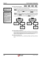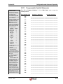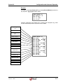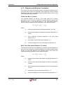
1
VOLUME 3B Fi rmwar eRevi si ons21. 74/ 25. 74 Omn i 3 0 0 0/ 6 0 0 0Fl o wCo mp u t e r Us e rMa n u a l Ef f ect i veJune2007 L i q u i dOr i f i c e/ Di f f e r e n t i a l Pr e s s u r eMe t e r s Volume 3b Configuration and Advanced Operation CONFIGURATION AND ADVANCED OPERATION Contents of Volume 3 Figures of Volume 3 ........................................................................................................... x About Our Company.......................................................................................................... xi Contacting Our Corporate Headquarters ........................................................................ xi Getting User Support ............................................................................................................. xi About the Flow Computer Applications ......................................................................... xii About the User Manual..................................................................................................... xii Target Audience..................................................................................................................... xii Manual Structure .................................................................................................................. xiii Volume 1. System Architecture and Installation ......................................................... xiii Volume 2. Basic Operation ......................................................................................... xiii Volume 3. Configuration and Advanced Operation ..................................................... xiii Volume 4. Modbus Database Addresses and Index Numbers ................................xiv Volume 5. Technical Bulletins .....................................................................................xiv Conventions Used in this Manual ....................................................................................... xiv Trademark References .......................................................................................................... xv Copyright Information and Modifications Policy............................................................... xvi Warranty, Licenses and Product Registration .............................................................. xvi 21/25.74+ 06/07 ® i OMNI 6000 / OMNI 3000 User Manual Contents of Volume 3 1. Overview of Firmware Revisions 21/25.74 ............................................................ 1-1 1.1. Number of Meter Runs - Type of Flowmeters ...................................................... 1-1 1.2. Product Configuration ........................................................................................... 1-2 1.3. Configurable Sensors per Meter Run................................................................... 1-2 1.4. Temperature, Pressure and Differential Pressure Transmitters ........................ 1-2 1.5. Densitometers ........................................................................................................ 1-2 1.6. Multivariable Flow Transmitters ........................................................................... 1-2 1.7. Station Capability ................................................................................................... 1-2 1.8. Auxiliary Inputs ...................................................................................................... 1-3 1.9. Number of Products - Information Stored per Product ...................................... 1-3 1.10. Orifice Flow Calculation Standards...................................................................... 1-3 1.11. Type of Products Measured .................................................................................. 1-3 1.12. Batching and Interface Detection ......................................................................... 1-3 1.13. PID Control Functions ........................................................................................... 1-4 1.14. Flow Weighted Averages ...................................................................................... 1-4 1.15. User-Programmable Digital I/O ............................................................................. 1-4 1.16. User-Programmable Logic Functions .................................................................. 1-4 1.17. User-Programmable Alarm Functions ................................................................. 1-4 1.18. User-Programmable Variables .............................................................................. 1-4 1.19. User Display Setups .............................................................................................. 1-4 1.20. User Report Templates .......................................................................................... 1-5 1.21. Serial Communication Links ................................................................................. 1-5 1.22. Peer-to-Peer Communications.............................................................................. 1-5 1.23. Archive Data ........................................................................................................... 1-5 ii 1.24. OmniCom Software Communications Package ............................................... 1-5 1.25. OmniView Software Communications Package ............................................... 1-5 ® 21/25.74+ 06/07 Volume 3b Configuration and Advanced Operation 2. Flow Computer Configuration ............................................................................... 2-1 2.1. Introduction ............................................................................................................ 2-1 2.2. Configuring with the Keypad in Program Mode .................................................. 2-1 2.2.1. Entering the Program Mode....................................................................................... 2-1 2.2.2. Changing Data ............................................................................................................ 2-1 2.2.3. Menu Selection Method.............................................................................................. 2-2 2.2.4. Random Access Method ............................................................................................ 2-2 Example: ..................................................................................................................... 2-2 2.2.5. Passwords ................................................................................................................... 2-3 Local Keypad Access.................................................................................................. 2-3 Changing Passwords at the Keypad........................................................................... 2-4 2.3. Getting Help ............................................................................................................ 2-4 2.4. Program Inhibit Switch .......................................................................................... 2-4 2.5. Configuring the Physical Inputs / Outputs ......................................................... 2-5 2.5.1. Miscellaneous I/O Configuration (Misc. Setup Menu) ............................................. 2-5 2.5.2. Physical I/O Points not Available for Configuration ............................................... 2-6 2.5.3. Password Maintenance Settings............................................................................... 2-6 2.5.4. I/O Module Settings .................................................................................................... 2-7 2.5.5. Meter Station I/O Assignments ................................................................................. 2-8 Auxiliary Input Assignment.......................................................................................... 2-9 2.5.6. Meter Run I/O Assignments ..................................................................................... 2-10 2.5.7. PID Control I/O Assignments................................................................................... 2-13 2.5.8. Analog Output Assignments ................................................................................... 2-15 2.5.9. Front Panel Counter Settings .................................................................................. 2-16 2.5.10.Programmable Boolean Statements ...................................................................... 2-17 2.5.11.Programmable Variable Statements ...................................................................... 2-19 2.5.12.User Display Settings .............................................................................................. 2-21 User Display #1 ......................................................................................................... 2-21 User Display #2 ......................................................................................................... 2-21 User Display #3 ......................................................................................................... 2-21 User Display #4 ......................................................................................................... 2-22 User Display #5 ......................................................................................................... 2-22 User Display #6 ......................................................................................................... 2-22 User Display #7 ......................................................................................................... 2-22 User Display #8 ......................................................................................................... 2-22 2.5.13.Digital I/O Point Settings ......................................................................................... 2-23 2.5.14.Serial Input / Output Settings ................................................................................ 2-25 21/25.74+ 06/07 ® iii OMNI 6000 / OMNI 3000 User Manual Contents of Volume 3 2.5.15.Peer-to-Peer Communications Settings ................................................................ 2-27 Transaction #1 .......................................................................................................... 2-28 Transaction #2 .......................................................................................................... 2-28 Transaction #3 .......................................................................................................... 2-28 Transaction #4 .......................................................................................................... 2-29 Transaction #5 .......................................................................................................... 2-29 Transaction #6 .......................................................................................................... 2-29 Transaction #7 .......................................................................................................... 2-29 Transaction #8 .......................................................................................................... 2-29 Transaction #9 .......................................................................................................... 2-30 Transaction #10 ........................................................................................................ 2-30 Transaction #11 ........................................................................................................ 2-30 Transaction #12 ........................................................................................................ 2-30 Transaction #13 ........................................................................................................ 2-30 Transaction #14 ........................................................................................................ 2-31 Transaction #15 ........................................................................................................ 2-31 Transaction #16 ........................................................................................................ 2-31 2.5.16.Custom Modbus Data Packet Settings ............................................................... 2-32 Custom Modbus Data Packet #1 (Addressed at 001) .............................................. 2-32 Custom Modbus Data Packet #2 (Addressed at 201) .............................................. 2-32 Custom Modbus Data Packet #3 (Addressed at 401) .............................................. 2-32 2.5.17.Programmable Logic Controller Setup ................................................................. 2-33 2.5.18.Archive File Setup ................................................................................................... 2-33 2.6. Setting Up the Time and Date ............................................................................. 2-34 2.6.1. Accessing the Time/Date Setup Submenu............................................................. 2-34 2.6.2. Time and Date Settings ............................................................................................ 2-34 2.7. Configuring the Meter Station............................................................................. 2-35 2.7.1. Accessing the Station Setup Submenu .................................................................. 2-35 2.7.2. Meter Station Settings .............................................................................................. 2-35 Auxiliary Inputs .......................................................................................................... 2-38 2.8. Configuring Meter Runs ...................................................................................... 2-39 2.8.1. Accessing the Meter Run Setup Submenu ............................................................ 2-39 2.8.2. Meter Run Settings ................................................................................................... 2-39 2.9. Configuring Meter Temperature ......................................................................... 2-42 2.9.1. Accessing the Temperature Setup Submenu ........................................................ 2-42 2.9.2. Meter Temperature Settings .................................................................................... 2-42 2.9.3. Meter Density Temperature Settings ...................................................................... 2-44 iv ® 21/25.74+ 06/07 Volume 3b Configuration and Advanced Operation 2.10. Configuring Meter Pressure ................................................................................ 2-45 2.10.1.Accessing the Pressure Setup Submenu ............................................................. 2-45 2.10.2.Meter Pressure Settings ......................................................................................... 2-45 2.10.3.Meter Density Pressure Settings ........................................................................... 2-47 2.11. Configuring Meter Relative Density (Specific Gravity) / Density ..................... 2-48 2.11.1.Accessing the Gravity/Density Setup Submenu .................................................. 2-48 2.11.2.Meter Relative Density / Density Settings ............................................................. 2-48 Relative Density / Density Data ................................................................................ 2-48 Digital Densitometer Factors .................................................................................... 2-50 2.12. Configuring PID Control Outputs ....................................................................... 2-52 2.12.1.Accessing the PID Control Setup Submenu ......................................................... 2-52 2.12.2.PID Control Output Settings ................................................................................... 2-52 Operating Mode ........................................................................................................ 2-52 Tuning Adjustments .................................................................................................. 2-53 Primary Controlled (Setpoint) Variable ..................................................................... 2-54 Secondary Controlled (Setpoint) Variable ................................................................ 2-54 2.13. Configuring Differential Pressure ....................................................................... 2-55 2.13.1.Accessing the Differential Pressure Setup Submenu ......................................... 2-55 2.13.2.Meter Differential Pressure Settings ..................................................................... 2-55 2.14. Configuring Products .......................................................................................... 2-58 2.14.1.Accessing the Fluid Data & Analysis Setup Submenu ........................................ 2-58 2.14.2.Product Settings ...................................................................................................... 2-58 Product #1 ................................................................................................................. 2-58 Product #2 ................................................................................................................. 2-59 Product #3 ................................................................................................................. 2-60 Product #4 ................................................................................................................. 2-60 Product #5 ................................................................................................................. 2-60 Product #6 ................................................................................................................. 2-61 Product #7 ................................................................................................................. 2-61 Product #8 ................................................................................................................. 2-61 Product #9 ................................................................................................................. 2-62 Product #10 ............................................................................................................... 2-62 Product #11 ............................................................................................................... 2-62 Product #12 ............................................................................................................... 2-63 Product #13 ............................................................................................................... 2-63 Product #14 ............................................................................................................... 2-63 Product #15 ............................................................................................................... 2-64 Product #16 ............................................................................................................... 2-64 2.15. Configuring Batches ............................................................................................ 2-65 21/25.74+ 06/07 ® v OMNI 6000 / OMNI 3000 User Manual Contents of Volume 3 2.16. Configuring Miscellaneous Factors ................................................................... 2-66 2.16.1.Accessing the Factor Setup Submenu .................................................................. 2-66 2.16.2.Factor Settings......................................................................................................... 2-66 Totalizer Rollover and Decimal Place Resolution ..................................................... 2-67 More Factors and System Constants ....................................................................... 2-67 2.17. Configuring Printers ............................................................................................ 2-68 2.17.1.Accessing the Printer Setup Submenu ................................................................. 2-68 2.17.2.Printer Settings ........................................................................................................ 2-68 3. User-Programmable Functions .............................................................................. 3-1 3.1. Introduction ............................................................................................................ 3-1 3.2. User-Programmable Boolean Flags and Statements ......................................... 3-1 3.2.1. What is a Boolean? ..................................................................................................... 3-1 Physical Digital I/O Points (1001 1024) .................................................................. 3-2 Programmable Boolean Points (1025 1088) .......................................................... 3-2 Programmable Accumulator Points (1089 One-Shot Boolean Points (1501 Scratch Pad Boolean Points (1650 1099) ................................................... 3-2 1649) .................................................................. 3-3 1699) .............................................................. 3-3 3.2.2. Sign (+, -) of Analog or Calculated Variables (5001 8999) ................................ 3-3 3.2.3. Boolean Statements and Functions ......................................................................... 3-3 Example 1: Meter Failure Alarm for Two-Meter Run Application ........................... 3-5 Example 2: Automatic Run Switching for 4-Meter Run Application ....................... 3-6 3.2.4. How the Digital I/O Assignments are Configured ................................................... 3-8 3.3. User Programmable Variables and Statements ................................................ 3-10 3.3.1. Variable Statements and Mathematical Operators Allowed ................................. 3-10 Example 1: ................................................................................................................ 3-11 Example 2: ................................................................................................................ 3-11 Example 3: ................................................................................................................ 3-12 Example 4: ................................................................................................................ 3-12 3.3.2. Using Boolean Variables in Variable Statements .................................................. 3-12 Example: ................................................................................................................... 3-12 3.3.3. Entering Values Directly into the User Variables .................................................. 3-13 3.3.4. Using the Variable Expression as a Prompt .......................................................... 3-13 3.3.5. Password Level Needed to Change the Value of a User Variable ....................... 3-13 3.3.6. Using Variables in Boolean Expressions ............................................................... 3-14 Example: ................................................................................................................... 3-14 3.4. User Configurable Display Screens ................................................................... 3-15 Example: ................................................................................................................... 3-17 vi ® 21/25.74+ 06/07 Volume 3b Configuration and Advanced Operation 4. Flow Equations and Algorithms for US Customary Units (Revision 21.74) ..... 4-1 4.1. Flow Rate for Liquid Orifice Metering .................................................................. 4-1 4.1.1. Mass Flow Rate at Flowing Conditions .................................................................... 4-1 ‟qm‟ (lbm/sec) ............................................................................................................... 4-1 ‟Qm‟ (Klbm/hr) .............................................................................................................. 4-1 4.1.2. Volumetric Gross Flow Rate at Flowing Conditions „Qv‟ (Bbl/hr) .......................... 4-1 4.1.3. Volumetric Net Flow Rate at Base Conditions „Qb‟ (Bbl/hr) ................................... 4-1 4.1.4. Nomenclature .............................................................................................................. 4-2 4.1.5. Diameters and Diameter Correlations ...................................................................... 4-3 Orifice Plate Bore „d‟ (inches) ..................................................................................... 4-3 Meter Tube (Pipe) Internal Diameter „D‟ (inches) ....................................................... 4-3 Diameter (Beta) Ratio „ ‟............................................................................................. 4-4 Pipe Reynolds Number „RD‟ and „Rd‟ ......................................................................... 4-4 4.1.6. Velocity of Approach Factor „Ev‟ .............................................................................. 4-5 4.1.7. Discharge Coefficients „Cd‟ ........................................................................................ 4-6 Orifice Flowmeters with Flange Taps (RG Equation) „Cd(FT)‟ .................................... 4-6 Orifice Flowmeters with Pipe Taps „Cd(PT)‟................................................................ 4-7 4.1.8. Fluid Expansion Factor „Y‟......................................................................................... 4-8 4.2. Densities and Other Properties of Liquids .......................................................... 4-9 4.2.1. Flowing Density „ f‟ for Crude Oil and Refined Products ....................................... 4-9 Volume Correction Factor „VCF‟ ................................................................................. 4-9 Correction Factor for Pressure on Liquid „CPL‟.......................................................... 4-10 4.2.2. Density Calculated from Digital Densitometer Output Frequency ...................... 4-11 Solartron Density (gm/cc) ...................................................................................... 4-11 Additional Equation for Velocity of Sound Effects (Solartron Only) ....................... 4-12 Sarasota Density (gm/cc).......................................................................................... 4-13 UGC Density (gm/cc) ................................................................................................ 4-14 4.3. Equations for Propylene, Ethane/Propane C3+ Mixes, and Ethylene ............. 4-15 4.3.1. Propylene Calculations ............................................................................................ 4-15 4.3.2. Density of Ethane/Propane C3+ Mixes ................................................................... 4-15 4.3.3. Physical Properties of Ethylene .............................................................................. 4-15 4.4. PID Control............................................................................................................ 4-16 4.4.1. Primary Variable error % „ep‟ ................................................................................... 4-16 Forward Action .......................................................................................................... 4-16 Reverse Action .......................................................................................................... 4-16 4.4.2. Secondary Variable error % „es‟............................................................................... 4-16 Forward Action .......................................................................................................... 4-16 Reverse Action .......................................................................................................... 4-16 21/25.74+ 06/07 ® vii OMNI 6000 / OMNI 3000 User Manual Contents of Volume 3 4.4.3. Control Output % „C0‟ (Before Startup Limit Function) ......................................... 4-16 Controlling on Primary Variable ................................................................................ 4-16 Controlling on Secondary Variable ........................................................................... 4-16 4.4.4. Integral Error „ e‟...................................................................................................... 4-16 Controlling on Primary Variable ................................................................................ 4-16 Controlling on Secondary Variable ........................................................................... 4-16 5. Flow Equations and Algorithms for SI (Metric) Units (Revision 25.74) ............. 5-1 5.1. Flow Rate for Liquid Differential Pressure Devices (Orifice, Nozzle and Venturi)................................................................................. 5-1 5.1.1. Mass Flow Rate at Flowing Conditions .................................................................... 5-1 „qm‟ (Kg/sec) ................................................................................................................ 5-1 „Qm‟ (tonne/hr) ............................................................................................................. 5-1 5.1.2. Volumetric Gross Flow Rate at Flowing Conditions „Qv‟ (m3/hr) ........................... 5-1 5.1.3. Volumetric Net Flow Rate at Base Conditions „Qb‟ (m3/hr)..................................... 5-1 5.1.4. Nomenclature .............................................................................................................. 5-2 5.1.5. Diameters and Diameter Correlations ...................................................................... 5-3 Orifice Plate Bore or Nozzle / Venturi Throat Diameter „d‟ (mm) ................................ 5-3 Meter Tube (Pipe) Internal Diameter „D‟ (mm)............................................................ 5-3 Diameter (Beta) Ratio „ ‟............................................................................................. 5-4 Pipe Reynolds Number „RD‟ ....................................................................................... 5-4 5.1.6. Coefficient of Discharge „C‟ ....................................................................................... 5-5 Coefficient of Discharge for Orifice Plates ‟C(OP)‟ ........................................................ 5-5 Coefficient of Discharge for ISA 1932 Nozzles „C(IN)‟ ............................................... 5-6 Coefficient of Discharge for Long Radius Nozzles „C(LN)‟ ......................................... 5-6 Coefficient of Discharge for Classical Venturi Tubes ................................................. 5-6 Coefficient of Discharge for Venturi Nozzles „C(VN)‟ ................................................. 5-7 5.1.7. Fluid Expansion Factor „ ‟ ......................................................................................... 5-8 Expansion Factor at Upstream Conditions „ 1‟............................................................ 5-8 5.2. Densities Calculated from Digital Densitometer Output Frequency ................. 5-9 5.2.1. Solartron Density (Kg/m3) ....................................................................................... 5-9 Uncompensated Density ............................................................................................. 5-9 Temperature Compensated Density ........................................................................... 5-9 Temperature and Pressure Compensated Density .................................................. 5-10 Additional Equation for Velocity of Sound Effects (Solartron Only) ....................... 5-10 3 5.2.2. Sarasota Density (Kg/m ) ......................................................................................... 5-11 5.2.3. UGC Density (Kg/m3) ................................................................................................ 5-12 Uncorrected Density ................................................................................................. 5-12 Corrected Density ..................................................................................................... 5-12 viii ® 21/25.74+ 06/07 Volume 3b Configuration and Advanced Operation 5.3. PID Control............................................................................................................ 5-13 5.3.1. Primary Variable error % „ep‟ ................................................................................... 5-13 Forward Action .......................................................................................................... 5-13 Reverse Action .......................................................................................................... 5-13 5.3.2. Secondary Variable error % „es‟............................................................................... 5-13 Forward Action .......................................................................................................... 5-13 Reverse Action .......................................................................................................... 5-13 5.3.3. Control Output % „C0‟ (Before Startup Limit Function)......................................... 5-13 Controlling on Primary Variable ................................................................................ 5-13 Controlling on Secondary Variable ........................................................................... 5-13 5.3.4. Integral Error „ e‟...................................................................................................... 5-13 Controlling on Primary Variable ................................................................................ 5-13 Controlling on Secondary Variable ........................................................................... 5-13 21/25.74+ 06/07 ® ix OMNI 6000 / OMNI 3000 User Manual Contents of Volume 3 Figures of Volume 3 Fig. 1-1. Typical Gas Flow Metering Configuration Using Turbine and Orifice Flowmeters .................... 1-1 Fig. 2-1. Figure Showing Program Inhibit Switch ..................................................................................... 2-4 Fig. 3-1. Figure Showing Automatic Four-Meter Flow Zone Thresholds ................................................. 3-6 Fig. 3-2. Figure Showing Four-Meter Run Valve Switching ..................................................................... 3-7 Fig. 3-3. Keypad Layout - A through Z Keys .......................................................................................... 3-16 x ® 21/25.74+ 06/07 Volume 3b Configuration and Advanced Operation About Our Company Measure the Difference! OMNI flow computers Our products are currently being used world-wide at: Offshore oil and gas production facilities Crude oil, refined products, LPG, NGL and gas transmission lines Storage, truck and marine loading/offloading terminals Refineries; petrochemical and cogeneration plants. OMNI Flow Computers, Inc. is the world‟s leading manufacturer and supplier of panel-mount custody transfer flow computers and controllers. Our mission is to continue to achieve higher levels of customer and user satisfaction by applying the basic company values: our people, our products and productivity. Our products have become the international flow computing standard. OMNI Flow Computers pursues a policy of product development and continuous improvement. As a result, our flow computers are considered the “brain” and “cash register” of liquid and gas flow metering systems. Our staff is knowledgeable and professional. They represent the energy, intelligence and strength of our company, adding value to our products and services. With the customer and user in mind, we are committed to quality in everything we do, devoting our efforts to deliver workmanship of high caliber. Teamwork with uncompromising integrity is our lifestyle. Contacting Our Corporate Headquarters OMNI Flow Computers, Inc. 12620 West Airport Ste #100 Sugar Land Texas 77478 Phone: 281-240-6161 Fax: 281-240-6162 World-wide Web Site: http://www.omniflow.com E-mail Addresses: [email protected] Getting User Support Technical and sales support is available world-wide through our corporate or authorized representative offices. If you require user support, please contact the location nearest you (see insert) or our corporate offices. Our staff and representatives will enthusiastically work with you to ensure the sound operation of your flow computer. 21/25.74+ 06/07 ® xi OMNI 6000 / OMNI 3000 User Manual For Your Information About the Flow Computer Applications OMNI 6000 and OMNI 3000 Flow Computers are integrable into the majority of liquid and gas flow measurement and control systems. The current firmware revisions of OMNI 6000/OMNI 3000 Flow Computers are: 20.74/24.74: Turbine/Positive Displacement/Coriolis Liquid Flow Metering Systems with K Factor Linearization (US/metric units) 21.74/25.74: Orifice/Differential Pressure Liquid Flow Metering Systems (US/metric units) 22.74/26.74: Turbine/Positive Displacement Liquid Flow Metering Systems with Meter Factor Linearization (US/metric units) 23.74/27.74: Orifice/Turbine Gas Flow Metering Systems (US/metric units) About the User Manual This manual applies to .74+ firmware revisions of OMNI 6000 and OMNI 3000 Flow Computers. It is structured into 5 volumes and is the principal part of your flow computer documentation. Target Audience As a user‟s reference guide, this manual is intended for a sophisticated audience with knowledge of liquid and gas flow measurement technology. Different user levels of technical know-how are considered in this manual. You need not be an expert to operate the flow computer or use certain portions of this manual. However, some flow computer features require a certain degree of expertise and/or advanced knowledge of liquid and gas flow instrumentation and electronic measurement. In general, each volume is directed towards the following users: Volume 1. System Architecture and Installation Installers System/Project Managers Engineers/Programmers Advanced Operators Operators Volume 2. Basic Operation All Users Volume 3. Configuration and Advanced Operation Engineers/Programmers Advanced Operators Volume 4. Modbus Database Addresses and Index Numbers Engineers/Programmers Advanced Operators Volume 5. Technical Bulletins Users with different levels of expertise. xii ® 21/25.74+ 06/07 Volume 3b Configuration and Advanced Operation Manual Structure The User Manual comprises 5 volumes; each contained in separate binding for easy manipulation. You will find a detailed table of contents at the beginning of each volume. Volume 1. System Architecture and Installation Volume 1 is generic to all applications and considers both US and metric units. This volume describes: Basic hardware/software features Installation practices Calibration procedures Flow computer specifications Volume 2. Basic Operation User Reference Documentation - The User Manual is structured into five volumes. Volumes 1 and 5 are generic to all flow computer application revisions. Volumes 2, 3 and 4 are application specific. These have four versions each, published in separate documents; i.e., one per application revision per volume. You will receive the version that corresponds to your application revision. The volumes respective to each application revision are: Revision 20/24.74: Volume #s 2a, 3a, 4a Revision 21/25.74: Volume #s 2b, 3b, 4b Revision 22/26.74: Volume #s 2c, 3c, 4c Revision 23/27.74: Volume #s 2d, 3d, 4d For example, if your flow computer application revision is 20/24.74, you will be supplied with 3a & 4a, along with Volumes 1, 2, & 5. Volume 2 is generic to all applications and considers both US and metric units. It covers the essential and routine tasks and procedures that may be performed by the flow computer operator. Both US and metric units are considered. General computer-related features are described, such as: The application-related topics may include: Batching operations Proving functions PID control functions Audit trail Other application specific functions Depending on your application, some of these topics may not be included in your specific documentation. An index of display variables and corresponding key press sequences that are specific to your application are listed at the end of each version of this volume. Volume 3. Configuration and Advanced Operation Volume 3 is intended for the advanced user. It refers to application specific topics and is available in four separate versions (one for each application revision). This volume covers: 21/25.74+ 06/07 Overview of keypad functions Adjusting the display Clearing and viewing alarms Computer totalizing Printing and customizing reports Application overview Flow computer configuration data entry User-programmable functions Modbus Protocol implementation Flow equations and algorithms ® xiii OMNI 6000 / OMNI 3000 User Manual Volume 4. Modbus For Your Information Database Addresses and Index Numbers Volume 4 is intended for the system programmer (advanced user). It comprises a descriptive list of database point assignments in numerical order, within our firmware. This volume is application specific, for which there is one version per application revision. Volume 5. Technical Bulletins Manual Updates and Technical Bulletins Volume 5 of the User Manual is a compendium of Technical Bulletins. They contain updates to the user manual. You can view and print updates from our website: http://www.omniflow.com Volume 5 includes technical bulletins that contain important complementary information about your flow computer hardware and software. Each bulletin covers a topic that may be generic to all applications or specific to a particular revision. They include product updates, theoretical descriptions, technical specifications, procedures, and other information of interest. This is the most dynamic and current volume. Technical bulletins may be added to this volume after its publication. You can view and print these bulletins from our website. Conventions Used in this Manual Typographical Conventions - These are standard graphical/text elements used to denote types of information. For your convenience, a few conventions where established in the manual‟s layout design. These highlight important information of interest to the reader and are easily caught by the eye. Several typographical conventions have been established as standard reference to highlight information that may be important to the reader. These will allow you to quickly identify distinct types of information. CONVENTION USED Sidebar Notes / InfoTips Example: INFO - Sidebar notes are used to highlight important information in a concise manner. Keys / Key Press Sequences Example: [Prog] [Batch] [Meter] [n] Screen Displays Example: Use Up/Down Arrows To Adjust Contrast; Left, Right Arrows To Adjust Backlight xiv DESCRIPTION Sidebar notes or “InfoTips” consist of concise information of interest which is enclosed in a grayshaded box placed on the left margin of a page. These refer to topics that are either next to them, or on the same or facing page. It is highly recommended that you read them. Keys on the flow computer keypad are denoted with brackets and bold face characters (e.g.: the „up arrow‟ key is denoted as []). The actual function of the key as it is labeled on the keypad is what appears between brackets. Key Press sequences that are executed from the flow computer keypad are expressed in a series of keys separated by a space (as shown in the example). Sample screens that correspond to the flow computer display appear surrounded by a dark gray border with the text in bold face characters and mono-spaced font. The flow computer display is actually 4 lines by 20 characters. Screens that are more than 4 lines must be scrolled to reveal the text shown in the manual. ® 21/25.74+ 06/07 Volume 3b Configuration and Advanced Operation CONVENTION USED Headings Example: 2. Chapter Heading 2.3. Section Heading 2.3.1. Subsection Heading Figure Captions Example: Fig. 2-3. Figure No. 3 of Chapter 2 Page Numbers Example: 2-8 Application Revision and Effective Publication Date Examples: All.74 06/07 20/24.74 06/07 21/25.74 06/07 22/26.74 06/07 23/27.73 06/07 DESCRIPTION Sequential heading numbering is used to categorize topics within each volume of the User Manual. The highest heading level is a chapter, which is divided into sections, which are likewise subdivided into subsections. Among other benefits, this facilitates information organization and cross-referencing. Figure captions are numbered in sequence as they appear in each chapter. The first number identifies the chapter, followed by the sequence number and title of the illustration. Page numbering restarts at the beginning of every chapter and technical bulletin. Page numbers are preceded by the chapter number followed by a hyphen. Technical bulletins only indicate the page number of that bulletin. Page numbers are located on the outside margin in the footer of each page. The contents of Volume 1 and Volume 5 are common to all application revisions and are denoted as All.74. Content of Volumes 2, 3 and 4 are application specific and are identified with the application number. These identifiers are included on every page in the inside margin of the footer, opposite the page number. The publication/effective date of the manual follows the application identification. The date is expressed as month/year (e.g.: June 2007 is 06/07). Trademark References The following are trademarks of OMNI Flow Computers, Inc.: OMNI 3000 OMNI 6000 OmniCom Other brand, product and company names that appear in this manual are trademarks of their respective owners. 21/25.74+ 06/07 ® xv OMNI 6000 / OMNI 3000 User Manual For Your Information Copyright Information and Modifications Policy This manual is copyright protected. All rights reserved. No part of this manual may be used or reproduced in any form, or stored in any database or retrieval system, without prior written consent of OMNI Flow Computers, Inc., Sugar Land, Texas, USA. Making copies of any part of this manual for any purpose other than your own personal use is a violation of United States copyright laws and international treaty provisions. OMNI Flow Computers, Inc., in conformance with its policy of product development and improvement, may make any necessary changes to this document without notice. Warranty, Licenses and Product Registration Product warranty and licenses for use of OMNI flow computer firmware and of OmniCom Configuration PC Software are included in the first pages of each Volume of this manual. We require that you read this information before using your OMNI flow computer and the supplied software and documentation. Important! If you have not done so already, please complete and return to us the product registration form included with your flow computer. We need this information for warranty purposes, to render you technical support and serve you in future upgrades. Registered users will also receive important updates and information about their flow computer and metering system. Copyright 1991-2007 by OMNI Flow Computers, Inc. All Rights Reserved. xvi ® 21/25.74+ 06/07 Volume 3b Configuration and Advanced Operation 1. Overview of Firmware Revisions 21/25.74 Orifice / Differential Pressure Liquid Flow Metering Systems 1.1. Number of Meter Runs - Type of Flowmeters Minimum 1 run, maximum 4 runs - orifice meters (stacked or unstacked). PID P D DP T T SP DP STREAM #1 PID P D DP T T SP DP STREAM #2 PID P D DP T T SP DP STREAM #3 PID P D DP T T SP DP STREAM #4 P D A A A A T PRODUCT INTERFACE DETECT Fig. 1-1. 21/25.74+ 06/07 AUXILIARY INPUTS Typical Liquid Flow Metering Configuration Using Orifice Flowmeters ® 1-1 Chapter 1 Overview of Firmware Revision 21.74 1.2. Product Configuration Parallel runs measuring the same product or independent runs with different products. 1.3. Configurable Sensors per Meter Run Differential pressure, meter temperature and pressure, meter density, densitometer temperature and pressure. 1.4. Temperature, Pressure and Differential Pressure Transmitters All transmitters can be either 4-20mA, 1-5V or Honeywell DE digital protocol types. In addition, temperature sensors can be directly connected as four wire DIN or American curve RTD probes connected directly. 1.5. Densitometers Can be configured for any combination or mix of individual or shared densitometers of any type (analog specific gravity, analog API density, analog density (grs/cc), digital Solartron pulse, digital Sarasota pulse or digital UGC pulse); the maximum number that can be connected is five. Each densitometer can be specified at either flowing or reference conditions. 1.6. Multivariable Flow Transmitters These special type of smart digital instrumentation devices (e.g.: Coriolis and ultrasonic liquid and gas flowmeters) incorporate multiple sensors that can be accessed by one or more flow computers. Up to four multivariable transmitters (one per meter run) can be connected to the OMNI flow computer. These devices use serial data communication links to transfer data to and from the flow computer, requiring an „SV‟ type combination module. Honeywell multivariable transmitters require an „HV‟ combo module. Point-to-point configurations and direct pulse trains are also acceptable connectivity options. 1.7. Station Capability Meter runs may be combined or subtracted in any mode to provide station flow rates and totalizers. These can be used in 'Check/Pay' meter systems to monitor flows and alarms, if deviations exceed a preset limit. 1-2 ® 21/25.74+ 06/07 Volume 3b Configuration and Advanced Operation 1.8. Auxiliary Inputs Four auxiliary inputs are provided for miscellaneous sensors (e.g.: BS&W, viscosity monitors, etc.), and can be individually selected to be 4-20mA or 4-wire RTD probe. 1.9. Number of Products - Information Stored per Product Information for sixteen different products can be stored. Product setup information includes: name, type of product, meter factors for each flowmeter, gravity/density override, and calculation algorithm to be used when running the product. 1.10. Orifice Flow Calculation Standards Orifice flow is calculated in conformance with AGA 3. 1.11. Type of Products Measured The products that can be measured are: Crude oil and refined products NGLs using API 2540 LPGs using GPA TP16, GPA TP27 Propylene using API 11.3.3.2 Ethylene using IUPAC/NIST 1045 or API 2565/API 11.3.2 Ethane-propane and C3+ mixes (SG: 0.350 - 0.660) using calculations based on GPA TP1 and TP2. Inferred mass calculation mode densitometers and volume flowmeters is also standard. 1.12. Batching and Interface Detection Six batch setups per meter run can be programmed with alphanumeric batch ID tag, product number to run, and expected size of batch. Individual meter run batch preset down counters provide 'batch end warning' and 'batch end reached' alarms. Batches can be ended manually or automatically on size of batch, change of product, beginning of new day, day of the week or day of the month. Product interface detection is achieved using a meter run densitometer or a separate station interface detector densitometer mounted ahead of the meter runs. Line pack count down counters allow up to three product interfaces to be tracked between the interface detector gravitometer and the valve manifold, allowing pre-emptive product cuts. 21/25.74+ 06/07 ® 1-3 Chapter 1 Overview of Firmware Revision 21.74 1.13. PID Control Functions Four independent control loops are provided for control of a primary variable with either high or low override control by a secondary variable. Contact closure inputs are activated to provide a startup and shutdown ramp function for each control loop, if needed. Primary setpoint can be adjusted via an analog input, a keypad entry, or communication link. Control loops are not dedicated and may be cascaded. Data is processed every 500 msec. 1.14. Flow Weighted Averages Flow weighted averages are calculated for all input variables and correction factors based on daily totals and running batch totals. 1.15. User-Programmable Digital I/O Each I/O point is individually configurable as either an input or output with variable 'delay on' and 'delay off'. Pulse widths are adjustable when used as auxiliary totalizer outputs or sampler outputs. 1.16. User-Programmable Logic Functions Sixty-four logic statements can be user-programmed to control meter run switching and provide user auxiliary control functions. 1.17. User-Programmable Alarm Functions Sixteen of the programmable logic statements described above can be used to contain custom text messages which can be displayed, logged and printed. 1.18. User-Programmable Variables Sixty-four user variables can be programmed to manipulate data for display and printing or remote access via a communication port. Typical uses include, special units conversions, customer averaging algorithms for leak detection, special limit checking and control functions. The programmable variable statements can also be used to type cast data of one type to another (i.e., change a floating point variable to an integer type so that a PLC or DCS system can make use of it). 1.19. User Display Setups The user may specify eight key press combinations which recall display screens. Each user display screen can show four variables each with a descriptive tag defined by the user. 1-4 ® 21/25.74+ 06/07 Volume 3b Configuration and Advanced Operation 1.20. User Report Templates Using OmniCom the user can generate custom report templates or edit existing templates. These are uploaded into the flow computer. Custom templates for the snapshot, batch end, daily and prove reports can be defined. 1.21. Serial Communication Links Up to six serial data links are available for communications with other devices such as printers, SCADA systems, PLC‟s and other OMNI flow computers. Ports communicate using a superset of the Modbus protocol (ASCII or RTU). Printer data is ASCII data. Baud rate is up to 38.4 Kbps. 1.22. Peer-to-Peer Communications OMNI flow computers can be user configured to communicate with each other as equal peers. Groups of data variables can be exchanged or broadcast between other flow computers. Multiple flow computers can share resources such as a PLC. 1.23. Archive Data Two types of data archiving are possible in the flow computer: (1) Formatted ASCII text using custom report templates, (2) Raw data using archive records and files. 1.24. OmniCom Package Software Communications OmniCom software is provided with each flow computer, and allows the user to configure the computer on-line or off-line using a personal computer. 1.25. OmniView Package Software Communications A Man-Machine Interface package for the OMNI Flow Computer is also available as an option. 21/25.74+ 06/07 ® 1-5 Chapter 1 1-6 Overview of Firmware Revision 21.74 ® 21/25.74+ 06/07 Volume 3b Configuration and Advanced Operation 2. Flow Computer Configuration 2.1. Introduction Configuration data is stored in the computer's battery backed-up RAM memory which will retain its data for at least 1 to 2 months with no power applied. Configuration data can be entered using one of three methods: 1) Configure off-line using the OmniCom then uploading all data at once. PC configuration program and 2) Configure on-line using the OmniCom PC configuration program which uploads each change as it is entered. 3) Enter configuration data via the front panel keypad using the Program Mode. Methods 1) and 2) require an IBM compatible PC running the OmniCom Configuration Software and are described in a Technical Bulletin on OmniCom (Volume 5) and in OmniCom Help. Method 3) is described here. 2.2. Configuring with the Keypad in Program Mode 2.2.1. Entering the Program Mode INFO - Key presses are denoted in bold face between brackets; e.g.: the enter key appears in this manual as [Enter]. th The 4 line of the display is used to show the user key presses. While in the Display Mode press the [Prog] key. The front panel Program LED above the key will glow green and the following selection menu will be displayed on the first three lines of the LCD display. Press Keys to Select Group Entry, or Press “Prog” to Exit 2.2.2. Changing Data Data can be accessed using a sequential list of menu prompts or in a random access manner by going directly to a specific group of entries. 21/25.74+ 06/07 ® 2-1 Chapter 2 Flow Computer Configuration 2.2.3. Menu Selection Method INFO - Characters in „[ ]‟ refer to key presses. *** SETUP MENU *** Misc Configuration _ Time/Date Setup Station Setup Meter Run Setup Temperature Setup Pressure Setup Grav/Density Setup PID Control Setup DP Inches of Water Product Setup Batch Preset Setup Batch Sequence Factor Setup Printer Setup TIP - It is best to use the menu selection method when programming an application for the first time as every possible option and variable will be prompted. Once a computer is in operation and you become familiar with the application you can decide to use the faster Random Access Method. To use the menu selection method, while in the Program Mode (program LED on) press [Setup] [Enter]. A Setup Menu similar to the one on the right will be displayed. Use the []/[] (up/down arrow) keys to move the cursor to the appropriate entry and press [Enter] to access a particular submenu. The first menu, 'Misc Configuration', should always be completed first as these entries specify the number and type of input and output devices connected to the flow computer; i.e., the menu items following the 'Misc Configuration' menu do not ask for configuration data unless a transducer has been defined. 2.2.4. Random Access Method In addition to the Setup Menu, the data is also presented in related groups such as Temperature, Pressure, Meter, etc. You press the group key of your choice to get to a data area. By specifying a meter run before or after a group you go directly to the data for that group and that group only. Once a group is selected use the 'Up/Down' arrow keys to step to a specific data entry within the group. You can view data and, assuming a valid password has been entered, change its value as required. If an error is made, press [Clear], re-enter the correct data and press [Enter] to enter the new value. The cursor will automatically step to the next data item in that group unless that would cause a total change of screen (i.e., you can always verify your entry). A list of data groups and associated key presses is listed later in this chapter. Example: Pressing [Temp] will allow you access to temperature data for all meter runs. Pressing [Meter] [1] [Temp] or [Temp] [Meter] [1] will allow access to only Meter Run #1 temperature data. For example, pressing [Meter] [1] [Temp] will display the following until the [Enter] key is pressed. th The 4 line of the display is used to show the user key presses. 2-2 Press Group Press Meter ® Keys to Select Entry, or “Prog” to Exit 1 Temp 21/25.74+ 06/07 Volume 3b Configuration and Advanced Operation Pressing the [Enter] key will display a screen similar to this: TEMPERATURE #1 Deg.F Low Limit 30.0 High Limit 125.0 Override 60.0 2.2.5. Passwords INFO - Most entry groups occupy multiple screens so be sure to use the []/[] to scroll and see all data. Except when changing transducer high/low alarm limits, a password is usually asked for when changing the configuration data within the computer. The flow computer has independent password protection of the following: Local Keypad Access / Modbus Port #1 (selectable) (Physical Serial Port #1) Modbus Port #2 - (Physical Serial Port #2) Modbus Port #3 - (Physical Serial Port #3) Modbus Port #4 - (Physical Serial Port #4) Local Keypad Access Three password levels are provided: Privileged Level Allows complete access to all entries within the flow computer including keypad passwords 1, 1A and 2 below. The initial privileged password for each Modbus port is selected via this password level. Level 1 This level allows technician access to most entries within the flow computer with the exception of I/O Points assignments, programmable variables and Boolean statements. Level 1A This level allows technician access to the following entries only: Densitometer Factor) Level 2 Correction Factors (Pycnometer Allows access to the operator type entries. These entries include: Transducer Manual Overrides Product Gravity Overrides Batching Operations 21/25.74+ 06/07 ® 2-3 Chapter 2 Flow Computer Configuration Changing Passwords at the Keypad INFO - Characters in „[ ]‟ refer to key presses. 1) At the keypad press [Prog] [Setup] [Enter]. 2) With the cursor blinking on 'Misc Configuration', press [Enter]. 3) With the cursor blinking on 'Password Maint?', press [Enter]. 4) Enter the Privileged Level Password (up to 6 Characters) and press [Enter]. 5) The Level 1, 1A and Level 2 passwords can now be viewed and changed if required. INFO - See Technical Bulletin TB-960701 in Volume 5 for setting Level B and Level C passwords using OmniCom. Note: Serial PortLevel B and Level C passwords for each Modbus port cannot be viewed or changed from the keypad. INFO - The Help System is not limited to just the Program Mode. Context sensitive help is available in all modes of operation. 1) Scroll down to access each of the Modbus serial port 'Level A' passwords. These are labeled „Serial 1 Passwd‟ (if Modbus Protocol is selected), 'Serial 2 Passwd', Serial 3 Passwd', and 'Serial 4 Passwd‟ corresponding to the physical port numbering for Modbus Ports 1, 2, 3 and 4. 2.3. Getting Help Context sensitive help is available for most data entries. Help is summoned by pressing the [Display/Enter/Help] key twice, within one second, with the cursor on the data field in question. Help screens are frequently more than 1 full screen so always use the []/[] keys to scroll in case there is more. Press [Prog] or [Enter] once to exit the help system and return to your original screen. 2.4. Program Inhibit Switch A 'Program Inhibit Switch' mounted behind the front panel prevents unauthorized changing of data when in the 'Inhibit' position. Most data can be viewed while the switch is in the program inhibit position, but any attempt to alter data will be ignored and cause 'PROGRAM LOCKOUT' to be displayed on the bottom line of the LCD display. The inner enclosure of the flow computer can be locked or sealed within the outer enclosure blocking access to the 'Program Inhibit Switch'. CAUTION! These units have an integral latching mechanism which first must be disengaged by lifting the bezel upwards before withdrawing the unit from the case. Fig. 2-1. 2-4 Figure Showing Program Inhibit Switch ® 21/25.74+ 06/07 Volume 3b Configuration and Advanced Operation 2.5. Tip - It is best to use the Menu Selection Method (see 2.2.3, this chapter) when programming an application for the first time as every possible option and variable will be prompted. Once a computer is in operation and you become familiar with the application you can decide to use the faster Random Access Method (see 2.2.4, this chapter). 2.5.1. INFO - Characters in „[ ]‟ refer to key presses. INFO - The first menu item, 'Misc Configuration', should always be completed first as these entries specify the number and type of input and output devices connected to the flow computer. You are advise to complete all entries under this menu before proceeding. Only transducers that have been assigned to physical I/O points will be available for further configuration (i.e., the menu items following the 'Misc Configuration' menu do not ask for or accept configuration data unless a transducer has been defined). (See 2.5.2, this chapter) 21/25.74+ 06/07 Configuring the Physical Inputs / Outputs The OMNI Flow Computer can accept many I/O modules and be configured to match just about any combination of measurement transmitters. Configuring the physical I/O means setting up the number of meter runs, what types of transducers are to be used and to which physical I/O points they are connected. Miscellaneous I/O Configuration (Misc. Setup Menu) The physical I/O configuration of the flow computer is changed by entering the „Misc. Setup‟ menu while the 'Select Group Entry' screen is displayed (see 9.2.1. “Entering the Program Mode”). Press Keys to Select Group Entry, or Press "Prog" to Exit Setup Press [Setup] then [Enter] and the following selection menu will be displayed: *** SETUP MENU *** Misc Configuration _ Time/Date Setup Station Setup The cursor automatically appears at the „Misc Configuration‟ option. Press [Enter] and the following selection menu will be displayed: *** Misc. Setup *** Password Maint?(Y) Check Modules ?(Y) Config Station?(Y) Config Meter “n” Config PID ? “n” Config D/A Out“n” Front Pnl Counters Program Booleans ? Program Variables? User Display ? “n” Config Digital“n” Serial I/O “n” Peer/Peer Comm(Y)? Custom Packet “n” Archive File “n” ® 2-5 Chapter 2 Flow Computer Configuration 2.5.2. Physical I/O Points not Available for Configuration Configuration parameter groups are only prompted as needed. Meter runs and transducers which are not assigned to a physical I/O point will not be available for configuration. In these cases the following message will be displayed: Variable Selected is Not Assigned to a Physical I/O Point If this message is displayed check the I/O point assignment for the variable. 2.5.3. Password Maintenance Settings INFO - Characters in ‟{ }‟ refer to password levels. Characters in „[ ]‟ refer to key presses. TIP - Use the blank lines provided next to each configuration option to write down the corresponding settings you entered in the flow computer. Some of these entries may not appear on the display or in OmniCom. Depending on the various configuration settings of your specific metering system, only those configuration options which are applicable will be displayed. Note: In the privileged password area all passwords are visible upon entering the correct privileged password. In all other cases when requested for a password, upon entering the password, the OMNI will display all entered characters as asterisk. 2-6 Enter [Y] at „Password Maint ?‟ of the „Misc Setup‟ menu to open the following entries: {PL} Privileged _______________ Enter the privileged password to allow you to view and change all configuration data including other passwords. {PL} Level 1 _______________ Enter the Level 1 password to allow entry of all configuration data except entries which determine the physical I/O personality of the computer. {PL} Level 1A _______________ Enter the Level 1A password to allow entry of Density Correction Factors only. {PL} Level 2 _______________ Enter the Level 2 password which is required for operator type entries such as gravity overrides and meter factors. {PL} Serial Port #1 Password _______________ Enter the Serial Port password. All data in the Modbus database except passwords can be read via the serial ports. These passwords allow writes to the Modbus database. Password protection can be disabled by entering a blank field as a password. {PL} Lockout Switch Active? N _______________ Enter [N] for the lockout switch to be inactive for this serial port. Enter [Y] for the lockout switch to be active for this serial port. {PL} Serial Port #2 Password _______________ Enter the Serial Port #2 Password. {PL} Lockout Switch Active? N _______________ {PL} Serial Port #3 Password _______________ {PL} Lockout Switch Active? N _______________ {PL} Serial Port #4 Password _______________ {PL} Lockout Switch Active? N _______________ {PL} Serial Port #5 Password _______________ {PL} Lockout Switch Active? N _______________ {PL} Serial Port #6 Password _______________ ® 21/25.74+ 06/07 Volume 3b Configuration and Advanced Operation INFO - Characters in ‟{ }‟ refer to password levels. Characters in „[ ]‟ refer to key presses. TIP - Use the blank lines provided next to each configuration option to write down the corresponding settings you entered in the flow computer. Some of these entries may not appear on the display or in OmniCom. Depending on the various configuration settings of your specific metering system, only those configuration options which are applicable will be displayed. CAUTION! If you change the number or type of installed I/O modules, you must perform the „Check Modules‟ Function to inform the computer that you wish to use the new hardware configuration. {PL} Lockout Switch Active? N _______________ {PL} Model # (0=3000, 1=6000) _______________ This entry is used by the OmniCom configuration software to determine the maximum I/O capability of the computer. Enter [0] to select OMNI 3000 or [1] to select OMNI 6000. {PL} Disable Download? _______________ Enter [Y] to disable OmniCom from downloading the configuration file to the OMNI flow computer. {PL} Reconfigure Archive _______________ Enter [Y] to reconfigure archive records definition. Enter [N] when finished. {PL} Archive Run (Y/N) _______________ Enter [Y] to start the archive running. {PL} Reset All Totalizers ? (Y/N) _______________ Reset All RAM and Reset Totalizers will only display after the privileged password has been entered. It will clear to zero all internal totalizers. You can change totalizer decimal place settings after entering [Y]. The three electromechanical totalizers on the front of the computer cannot be zeroed. {PL} Reset All RAM ? (Y/N) _______________ Resetting all RAM will clear all configuration data, calibration data and totalizers. This means that all configuration data will have to be re-entered. {PL} Input Calibrate Default ? _______________ Entering a [Y] here will set all the analog input calibration constants used to scale zero and span settings to the default value. This will require you to re calibrate all the inputs. You can also do this on a channel by channel basis by entering the input channel number. {PL} D/A Calibrate Default ? _______________ Entering a [Y] here will set all the analog output calibration constants used to scale zero and span settings to the default value. This will require you to re-calibrate all the outputs. You can also do this on a channel by channel basis by entering the output channel number. 2.5.4. I/O Module Settings Enter [Y] at „Check Modules ?‟ of the „Misc Setup‟ menu and a screen similar to the following will display: MODULE S-WARE H-WARE A-1 Y Y B-1 Y Y D-2 Y Y S-2 Y Y Update S-Ware ? {PL} Update S-Ware ? (Y) _______________ A table is displayed showing all of the physically installed I/O modules versus the I/O modules recognized by the software (see display example above). You must answer the 'Update Software' question entering [Y] whenever you change the number or type of installed modules. The available I/O point numbers are allocated to each module at this time according to the type and number of each module (see Volume 1 for more information). 21/25.74+ 06/07 ® 2-7 Chapter 2 Flow Computer Configuration 2.5.5. Meter Station I/O Assignments INFO - The number of process variable I/O points available depends on the number of combo modules installed (see Chapter 2 in Volume 1 for more information). Point numbers range from 01 through 24. Assign [0] to „invalidate the assigning of a variable. Enter [Y] at „Config Station ?‟ of the „Misc Setup‟ menu to open the following entries: {PL} Station Configured As: _______________ Station Totals and Flows Defined As: Define which meter runs will be included in the station flow rates and totalizers. Meter data can be added or subtracted. Example: Entering [1] [+] [2] [-] [3] [-] [4] defines the station flows and totals as the result of Meter Runs #1 and #2 added together, subtracted by the flows of Meters #3 and #4. Enter [0] for no station totalizers. I/O Type Mismatch - The computer will not let you assign the same I/O point # to incompatible transducer types; i.e., an I/O point cannot be assigned as a temperature input for Meter Run #1 and a pressure input for Meter Run #2. If the „I/O Type Mismatch‟ message is displayed, recheck the I/O. Shared Transducers Enter the same I/O point to share transducers between meter runs. Correcting a Mistake Enter an I/O point # of [0] to cancel an incorrectly entered I/O point #, then enter the correct number. Assigning I/O Point #99 This indicates that the associated variable will be available for display and be used in all calculations, but will not be obtained via a live input. The variable value is usually downloaded into the flow computer database via a communication port or via a user variable statement. {PL} Density I/O Point # _______________ Enter the I/O point number that corresponds to the station density or gravity input used as the product interface detector. Digital densitometers can be corrected for temperature and pressure effects using the station pressure and temperature points. Digital pulse th densitometers can only be assigned I/O point numbers corresponding to the 4 input channel of a B Type Combo Module, or Channels 3 or 4 of an E/D Type Combo Module. Density Tag _______________ Enter the 8-character tag name used to identify this density transducer on the LCD display. Enter Density Type _______________ Enter the densitometer type: 0 = No density type selected 1 = 4-20mA output signal linear with API gravity units (many API devices are actually designed to drive non-linear API chart recorders; they are usually linear with relative density units) 2 = 4-20mA output signal linear with relative density (SG) units 3 = 4-20mA output signal linear with grs/cc density 4 = Solartron digital pulse, 5=Sarasota digital pulse, 6=UGC digital pulse. {PL} Temperature I/O Point # _______________ Enter the I/O point number to which the temperature sensor used to compensate the station densitometer is connected. When a digital densitometer is used as the station transducer, it can be corrected for temperature effects by assigning a temperature I/O point. For the station product interface densitometer, enter a meter run temperature sensor in cases where a separate temperature transmitter is not available. st RTD probes should be assigned to the 1 channel on A, B, E/D or E type combo modules. nd RTD probes can also be assigned to the 2 channel of these combo modules. Temperature Transducer Tag _______________ Enter the 8-character tag name used to identify this temperature transducer on the LCD display. Temp Type (0=DIN,1=AM,2=4-20) _______________ Enter the densitometer temperature transmitter type: 0 = RTD Probes that follow a DIN curve and = 0.0385 1 = RTD Probes that follow an American curve and = 0. 0392 2 = Honeywell smart transmitter connected to an „H‟ combo module or a transducer with a 4-20mA linear output. 2-8 ® 21/25.74+ 06/07 Volume 3b Configuration and Advanced Operation {PL} Pressure I/O Point # INFO - Characters in ‟{ }‟ refer to password levels. Characters in „[ ]‟ refer to key presses. _______________ Enter the I/O point number to which the pressure transmitter used to compensate the station digital densitometers is connected. When a digital densitometer is used as the product interface detector, it can be corrected for pressure effects by assigning a station pressure point. If a separate pressure transmitter is not available, enter a meter pressure transmitter I/O point. TIP - Use the blank lines provided next to each configuration option to write down the corresponding settings you entered in the flow computer. Some of these entries may not appear on the display or in OmniCom. Depending on the various configuration settings of your specific metering system, only those configuration options which are applicable will be displayed. Pressure Transducer Tag _______________ Enter the 8-character tag name used to identify this pressure transducer on the LCD display. Auxiliary Input Assignment {PL} Auxiliary Input #1 I/O Point # _______________ Enter the physical I/O point number to which this auxiliary input is connected. Auxiliary Inputs can be used to enter miscellaneous variables. Auxiliary Input #1 Tag _______________ Enter the 8-character tag name used to identify this transducer on the LCD display. Auxiliary Input Type _______________ Enter the Auxiliary Input Type: 0 = RTD Probes that follow a DIN curve and = 0.0385 1 = RTD Probes that follow an American curve and = 0. 0392 2 = Honeywell smart transmitter connected to an „H‟ combo module or a transducer with a 4-20mA linear output. {PL} Auxiliary Input #2 I/O Point # _______________ Auxiliary Input #2 Tag _______________ Auxiliary Input Type _______________ {PL} Auxiliary Input #3 I/O Point # _______________ Auxiliary Input #3 Tag _______________ Auxiliary Input Type _______________ {PL} Auxiliary Input #4 I/O Point # 21/25.74+ 06/07 _______________ Auxiliary Input #4 Tag _______________ Auxiliary Input Type _______________ ® 2-9 Chapter 2 Flow Computer Configuration 2.5.6. Meter Run I/O Assignments Config Meter Runs Physical I/O information for up to 4 meter runs can be entered. Transducers that are not assigned an I/O point will not be available for display or further configuration. INFO - The number of process variable I/O points available depends on the number of combo modules installed (see Chapter 2 in Volume 1 for more information). Point numbers range from 01 through 24. Assign [0] to „invalidate the assigning of a variable. I/O Type Mismatch - The computer will not let you assign the same I/O point # to incompatible transducer types; i.e., an I/O point cannot be assigned as a temperature input for Meter Run #1 and a pressure input for Meter Run #2. If the „I/O Type Mismatch‟ message is displayed, recheck the I/O. Shared Transducers Enter the same I/O point to share transducers between meter runs. Correcting a Mistake Enter an I/O point # of [0] to cancel an incorrectly entered I/O point #, then enter the correct number. Assigning I/O Point #99 This indicates that the associated variable will be available for display and be used in all calculations, but will not be obtained via a live input. The variable value is usually downloaded into the flow computer database via a communication port or via a user variable statement. Enter [1], [2], [3] or [4] at „Config Meter "n"‟ of the „Misc Setup‟ menu to open the following entries: {PL} Select Device Type _______________ Each meter run may use either differential pressure (orifice) or multivariable transmitter. Enter one of the following to select your device type: 0 = differential pressure (orifice) flowmeter 1 = Rosemount 3095FB multivariable transmitter connected to an „SV‟ combo module (see TB-980501 “Rosemount 3095FB Multivariable Sensor Issues”) 2 = Honeywell SMV3000 multivariable transmitter connected to an „HV‟ combo module (see TB-980502 “Communicating with Honeywell SMV3000 Multivariable Transmitters”) {PL} SV Module Port # Meter #1 Meter #2 Meter #3 Meter #4 _______ _______ _______ _______ 3095FB This entry only appears when the device type selected is a Rosemount multivariable transmitter. Enter the port number of the SV combo module that is connected to this Rosemount 3095FB multivariable transmitter. Port numbers 1 and 2 are on the SV-1 combo module. Port numbers 3 and 4 are on the SV-2 combo module. SV ports can be connected to multiple 3095FB multivariables as long as each 3095FB has its own unique Modbus ID. {PL} SV Modbus ID _______ _______ _______ _______ This entry only appears when the device type selected is a Rosemount 3095FB multivariable transmitter. Each Rosemount 3095FB multivariable transmitter connected to a SV combo module port must have a unique Modbus ID. Enter the unique Modbus ID of the 3095FB transmitter which will be providing differential pressure, temperature and pressure for each corresponding meter run. {PL} DP (Low Range) I/O Point # _______ _______ _______ _______ Enter the I/O point used to input the signal from the differential pressure or multivariable sensor for each applicable meter run, according to the following: In the case of stacked DP installations, enter the I/O point to be used for the low range cell. When the device type is a Honeywell SMV3000 transmitter, entering an I/O point in this field will cause the OMNI to automatically assign I/O points for the meter run temperature and pressure variables. The assigned I/O points cannot be changed by the user. When Rosemount 3095FB multivariable transmitters are used no entry is needed as the flow computer automatically assigns these I/O points. Duplicate I/O assignments can be made when a transducer is shared between meter runs. (e.g.: forward and reverse flow). DP (Low Range) Tag _______ _______ _______ _______ Enter the 8-character tag name used to identify this transducer on the LCD display. {PL} DP High Range I/O Point # _______ _______ _______ _______ This entry applies only when device type „0‟ is selected. Enter the I/O point used to input the signal from the high range differential pressure (DP) signal for this meter run. Duplicate I/O assignments can be made when a transducer is shared between meter runs. (e.g.: forward and reverse flow). Enter [0] if stacked DP transmitters are not used. DP High Range Tag _______ _______ _______ _______ Enter the 8-character tag name used to identify this transducer on the LCD display. 2-10 ® 21/25.74+ 06/07 Volume 3b INFO - Characters in ‟{ }‟ refer to password levels. Characters in „[ ]‟ refer to key presses. TIP - Use the blank lines provided next to each configuration option to write down the corresponding settings you entered in the flow computer. Some of these entries may not appear on the display or in OmniCom. Depending on the various configuration settings of your specific metering system, only those configuration options which are applicable will be displayed. Configuration and Advanced Operation {PL} Temperature I/O Point # Meter #1 Meter #2 Meter #3 Meter #4 _______ _______ _______ _______ Enter the I/O point number used to input the temperature signal for each meter run. Duplicate I/O assignments are allowed when a sensor is shared by more than one meter run. When Honeywell SMV3000 multivariable transmitters are used, this I/O point is automatically assigned by the flow computer when the DP I/O point is assigned. It cannot be changed by the user. When 3095FB multivariable transmitters are used, this I/O point is automatically assigned by the flow computer and need not be entered by the user. Temperature Transducer Tag _______ _______ _______ _______ Enter the 8-character tag name used to identify this temperature transducer on the LCD display. Temp Transducer Type _______ _______ _______ _______ Enter the Temperature Transmitter Type: 0 = RTD Probes that follow a DIN curve and = 0.0385 1 = RTD Probes that follow an American curve and = 0. 0392 2 = Honeywell smart transmitter connected to an „H‟ combo module or a transducer with a 4-20mA linear output. {PL} Pressure I/O Point # _______ _______ _______ _______ Enter the I/O point number used to input the pressure signal for each meter run. Duplicate I/O assignments are allowed when a sensor is shared by more than one meter run. When Honeywell SMV3000 multivariable transmitters are used, this I/O point is automatically assigned by the flow computer when the DP I/O point is assigned. It cannot be changed by the user. When 3095FB multivariable transmitters are used, this I/O point is automatically assigned by the flow computer and need not be entered by the user. Pressure Transducer Tag _______ _______ _______ _______ Enter the 8-character tag name used to identify this pressure transducer on the LCD display. {PL} Density I/O Point # _______ _______ _______ _______ Enter the I/O point number used to input the density signal for each corresponding meter run. Duplicate I/O assignments are allowed when a densitometer is shared by more than one meter run. Digital pulse densitometers can only be assigned I/O point numbers corresponding to the th rd th 4 input channel of a B type Combo Module or the 3 and 4 input channels of an E/D combo module. Density Transducer Tag _______ _______ _______ _______ Enter the 8-character tag name used to identify this density transducer on the LCD display. Densitometer Type _______ _______ _______ _______ Enter the densitometer type: 0 = No density type selected 1 = 4-20mA output signal linear with API gravity units (many API devices are actually designed to drive non-linear API chart recorders; they are usually linear with relative density units) 2 = 4-20mA output signal linear with relative density (SG) units 3 = 4-20mA output signal linear with grs/cc density 4 = Solartron digital pulse 5 = Sarasota digital pulse 6 = UGC digital pulse. 21/25.74+ 06/07 ® 2-11 Chapter 2 Flow Computer Configuration Meter #1 Meter #2 Meter #3 Meter #4 {PL} Dens Temperature I/O Point # _______ _______ _______ _______ Enter the I/O point number used to input the signal applied to compensate for temperature effects at the densitometer for each meter run. If the densitometer has no temperature sensor fitted, enter the same I/O point assignment as the meter run temperature sensor. Dens Temp Transmitter Tag _______ _______ _______ _______ Enter the 8-character tag name used to identify this density temperature transducer on the LCD display. Dens Temp Transmitter Type _______ _______ _______ _______ Enter the Densitometer Temperature Transmitter Type: 0 = RTD Probes that follow a DIN curve and = 0.0385 1 = RTD Probes that follow an American curve and = 0.0392 2 = Honeywell smart transmitter connected to an „H‟ combo module or a transducer with a 4-20mA linear output. {PL} Dens Pressure I/O Point # _______ _______ _______ _______ Enter the I/O point number used to input the signal applied to compensate for pressure effects at the densitometer for each meter run. If the densitometer has no pressure sensor fitted, enter the same I/O point assignment as the meter run pressure sensor. Dens Press Transducer Tag _______ _______ _______ _______ Enter the 8-character tag name used to identify this density pressure transducer on the LCD display. 2-12 ® 21/25.74+ 06/07 Volume 3b Configuration and Advanced Operation 2.5.7. PID Control I/O Assignments Proportional Integral Derivative (PID) -- For practical reasons we refer to PID Control Loops in this manual. However, your flow computer actually performs the Proportional Integral (PI) function and does not apply the derivative term. The addition of the derivative term would greatly complicate tuning of the control loop and besides is not normally applicable to the types of flow and pressure control used in pipelines. Valid Assignments for Primary and Secondary Variables - Any integer or floating point variable within the database can be assigned to be the primary or secondary controlled variable (see Volume 4 for a complete listing of database addresses and index numbers). Enter [1], [2], [3] or [4] at „Config PID ? "n"‟ of the „Misc Setup‟ menu to open the following entries: {PL} Assign Primary Variable Loop #1 Loop #2 Loop #3 Loop #4 _______ _______ _______ _______ Enter the database index number of the primary variable in the PID loop (see the sidebar). Remark ____________ ____________ ____________ ____________ Enter a remark in this 16-character field which identifies and documents the function of each variable assignment. Action (Forward/Reverse) _______ _______ _______ _______ Enter [F] (forward action) if the value of the primary variable increases as the controller output % increases. Enter [R] (reverse action) if the value of the primary variable decreases as the controller output % increases. {PL} Remote Setpoint I/O Point # _______ _______ _______ _______ Enter the I/O point number that the remote set point analog input signal is connected to (0124). Assign this point to 99 in cases where the set point will be downloaded via a communication port. Enter [0] if you will not be using a remote setpoint. {PL} Assign Secondary Variable _______ _______ _______ _______ Enter the database index number of the secondary variable in the PID loop (see the sidebar). Remark ____________ ____________ ____________ ____________ Enter a remark in this 16-character field which identifies and documents the function of each variable assignment. Action (Forward/Reverse) _______ _______ _______ _______ Enter [F] (forward action) if the value of the primary variable increases as the controller output % increases. Enter [R] (reverse action) if the value of the primary variable decreases as the controller output % increases. 21/25.74+ 06/07 ® 2-13 Chapter 2 Flow Computer Configuration {PL} Error Select (Low/High) INFO - Characters in ‟{ }‟ refer to password levels. Characters in „[ ]‟ refer to key presses. TIP - Use the blank lines provided next to each configuration option to write down the corresponding settings you entered in the flow computer. Some of these entries may not appear on the display or in OmniCom. Depending on the various configuration settings of your specific metering system, only those configuration options which are applicable will be displayed. Loop #1 Loop #2 Loop #3 Loop #4 _______ _______ _______ _______ This entry is used to determine under what circumstances the primary or secondary variable is to be controlled. There are two modes of low/high error select: Mode #1: The controller will attempt to control the primary variable but will switch to controlling the secondary variable, should the controller be trying to drive the secondary variable ABOVE its setpoint. An example of this mode would be controlling flow rate (primary) while not exceeding a MAXIMUM delivery pressure (secondary). Mode #2: The controller will attempt to control primary variable but will switch to controlling the secondary variable, should the controller be trying to drive the secondary variable BELOW its setpoint. An example of this mode would be controlling flow rate (primary) while not dropping below a MINIMUM pressure value (secondary). Considering these modes, select your entry according to the following flow diagram. MODE #1 MODE #2 Are both primary and secondary actions forward? Are both primary and secondary actions forward? yes Enter [L] (Low Error Select) yes no yes Is secondary action forward? Enter [H] (High Error Select) no yes Is secondary action forward? no no Enter [H] (High Error Select) {PL} Startup Mode (Last/Manual) Enter [L] (Low Error Select) _______ _______ _______ _______ This entry determines how the computer handles a system reset such as a momentary loss of power. Enter [L] (Last) to cause the PID loop to stay in the operating mode it was last in before the system reset. Enter [M] (Manual) to cause the PID loop to startup with the PID loop in manual control mode and with the valve open % as it was before the system reset. {PL} PID Control Output Tag _______ _______ _______ _______ Enter an 8-character tag name used to identify the PID controller output % signal on the LCD display. 2-14 ® 21/25.74+ 06/07 Volume 3b Configuration and Advanced Operation 2.5.8. Analog Output Assignments INFO - Characters in ‟{ }‟ refer to password levels. Characters in „[ ]‟ refer to key presses. TIP - Use the blank lines provided next to each configuration option to write down the corresponding settings you entered in the flow computer. Some of these entries may not appear on the display or in OmniCom. Depending on the various configuration settings of your specific metering system, only those configuration options which are applicable will be displayed. Press [n] [Enter] at „Config D/A Out "n"‟ of the „Misc Setup‟ menu to open the following entries (n = D/A Output #): {L1} Analog Output #1 Assign at 4mA at 20mA __________ __________ __________ Under „Assign‟, enter the database index number of the variable that will be assigned to the digital-to-analog output points. Under „at 4mA‟ and „at 20mA‟, enter the required scaling parameters in engineering units at 4mA and 20mA (e.g.: For Meter #1 Net Flow Rate assign 7102. Typical scaling might be 4mA=0.0 Bbls/hr and 20mA=1000.0 Bbls/hr). Remark _______________ Enter a remark in this 16-character field which identifies and documents the function of each digital-to-analog output. {L1} Analog Output #2 __________ Remark {L1} Analog Output #3 __________ __________ __________ __________ __________ __________ __________ __________ __________ __________ __________ __________ __________ __________ __________ __________ __________ __________ __________ __________ __________ _______________ __________ Remark 21/25.74+ 06/07 __________ _______________ Remark {L1} Analog Output #13 __________ _______________ Remark {L1} Analog Output #12 __________ _______________ Remark {L1} Analog Output #11 __________ _______________ Remark {L1} Analog Output #10 __________ _______________ Remark {L1} Analog Output #9 __________ _______________ Remark {L1} Analog Output #8 __________ _______________ Remark {L1} Analog Output #7 __________ _______________ Remark {L1} Analog Output #6 __________ _______________ Remark {L1} Analog Output #5 __________ _______________ Remark {L1} Analog Output #4 __________ __________ __________ _______________ ® 2-15 Chapter 2 Flow Computer Configuration {L1} Analog Output #14 Assign at 4mA at 20mA __________ __________ __________ Remark {L1} Analog Output #15 _______________ __________ Remark {L1} Analog Output #16 __________ __________ __________ _______________ __________ Remark {L1} Analog Output #18 __________ _______________ Remark {L1} Analog Output #17 __________ __________ __________ _______________ __________ Remark __________ __________ _______________ 2.5.9. Front Panel Counter Settings Enter [Y] at „Front Pnl Counters‟ of the „Misc Setup‟ menu to open the following entries: Counter A {L1} Assign Front Panel Counter__________ Counter B Counter C __________ __________ Enter the database index number of the accumulator variable that will be output to this electromechanical counter. The unit of measure is the same as that shown on the LCD for the totalizer (i.e., barrels, klbs, 3 m , etc.) The maximum count rate is limited to 10 counts per second. Count rates higher than 10 pulses per second will cause the computer to remember how many counts did not get output and continue to output after the flow stops until all buffered counts are output. Remark ____________ ____________ ____________ Enter a remark in this 16-character field which identifies and documents the function of each front panel counter. Pulses/Unit __________ __________ __________ Enter the number of pulses per unit (volume, mass). 2-16 ® 21/25.74+ 06/07 Volume 3b Configuration and Advanced Operation 2.5.10. Programmable Boolean Statements Program Booleans - These 64 Boolean statements are evaluated every 100 msec starting at Point 1025 continuing through 1088. Each statement can contain up to 3 Boolean variables, optionally preceded by the slash (/) denoting the NOT Function and separated by a valid Boolean operator: Operator Symbol NOT / AND & OR + EXOR * EQUAL = IF ) GOTO G MOVE : COMPARE % Example: 1025:1002&/1003 Boolean 1025 is true when point 1002 is true AND point 1003 is NOT true. Note: Points 1002 and 1003 in this example reflect the status of Physical I/O Points 2 and 3. There are no limitations as to what Boolean points can be used in a statement. Statements can contain the results from other statements. Example: 1026: /1025+1105 Boolean 1026 is true when Boolean 1025 is NOT true OR Point 1105 is true. Using the „=‟ operator, the result of a statement can initiate a command. Example: 1027: 1719=1026 Request a „Snapshot Report‟ when Boolean 1026 is true. Note: See Volume 4 for detailed list of Booleans and Status Commands. 21/25.74+ 06/07 Enter [Y] at „Program Booleans ?‟ of the „Misc Setup‟ menu to open the following entries: Boolean Point 10xx Equation or Statement Comment or Remark 25: _______________________ _______________________ 26: _______________________ _______________________ 27: _______________________ _______________________ 28: _______________________ _______________________ 29: _______________________ _______________________ 30: _______________________ _______________________ 31: _______________________ _______________________ 32: _______________________ _______________________ 33: _______________________ _______________________ 34: _______________________ _______________________ 35: _______________________ _______________________ 36: _______________________ _______________________ 37: _______________________ _______________________ 38: _______________________ _______________________ 39: _______________________ _______________________ 40: _______________________ _______________________ 41: _______________________ _______________________ 42: _______________________ _______________________ 43: _______________________ _______________________ 44: _______________________ _______________________ 45: _______________________ _______________________ 46: _______________________ _______________________ 47: _______________________ _______________________ 48: _______________________ _______________________ 49: _______________________ _______________________ 50: _______________________ _______________________ 51: _______________________ _______________________ 52: _______________________ _______________________ 53: _______________________ _______________________ 54: _______________________ _______________________ 55: _______________________ _______________________ ® 2-17 Chapter 2 Flow Computer Configuration Boolean Point 10xx Equation or Statement Comment or Remark TIP - Use the blank lines provided next to each configuration option to write down the corresponding settings you entered in the flow computer. 56: _______________________ _______________________ 57: _______________________ _______________________ 58: _______________________ _______________________ 59: _______________________ _______________________ Program Booleans - These 64 Boolean statements are evaluated every 100 msec starting at Point 1025 continuing through 1088. Each statement can contain up to 3 Boolean variables, optionally preceded by the slash (/) denoting the NOT Function and separated by a valid Boolean operator: Operator Symbol NOT / AND & OR + EXOR * EQUAL = IF ) GOTO G MOVE : COMPARE % 60: _______________________ _______________________ 61: _______________________ _______________________ 62: _______________________ _______________________ 63: _______________________ _______________________ 64: _______________________ _______________________ 65: _______________________ _______________________ 66: _______________________ _______________________ 67: _______________________ _______________________ 68: _______________________ _______________________ 69: _______________________ _______________________ 70: _______________________ _______________________ 71: _______________________ _______________________ Example: 1025:1002&/1003 Boolean 1025 is true when point 1002 is true AND point 1003 is NOT true. Note: Points 1002 and 1003 in this example reflect the status of Physical I/O Points 2 and 3. There are no limitations as to what Boolean points can be used in a statement. Statements can contain the results from other statements. Example: 1026: /1025+1105 Boolean 1026 is true when Boolean 1025 is NOT true OR Point 1105 is true. Using the „=‟ operator, the result of a statement can initiate a command. Example: 1027: 1719=1026 Request a „Snapshot Report‟ when Boolean 1026 is true. 72: _______________________ _______________________ 73: _______________________ _______________________ 74: _______________________ _______________________ 75: _______________________ _______________________ 76: _______________________ _______________________ 77: _______________________ _______________________ 78: _______________________ _______________________ 79: _______________________ _______________________ 80: _______________________ _______________________ 81: _______________________ _______________________ 82: _______________________ _______________________ 83: _______________________ _______________________ 84: _______________________ _______________________ 85: _______________________ _______________________ 86: _______________________ _______________________ 87: _______________________ _______________________ 88: _______________________ _______________________ 2-18 ® 21/25.74+ 06/07 Volume 3b Configuration and Advanced Operation 2.5.11. Programmable Variable Statements Programmable Variables These 64 variable statements are evaluated every 500 msec starting at the statement that determines the value of Points 7025 through 7088. Each statement can contain up to 3 variables or constants. Variables can be optionally preceded by the „$‟ symbol denoting the ABSOLUTE value of the variable is to be used. Constants are identified by placing a ‟#‟ symbol ahead of the number. These and other operators are: Operator Symbol ABSOLUTE $ CONSTANT # POWER & MULTIPLY * DIVIDE / ADD + SUBTRACT EQUAL = IF ) GOTO G MOVE : COMPARE % INDIRECT “ The order of precedence is: 1) ABSOLUTE 2) POWER 3) MULTIPLY/DIVIDE 4) ADD/SUBTRACT In cases where operators have the same precedence, statements are evaluated left to right. E.g.: The value of floating point variable 7035 is defined as: 7035:7027�.5*7026 The power operator is evaluated first (the value of Point 7035 is set equal to the square root of the number contained in Point 7027) and the result is multiplied by the number stored in variable 7026. Note that statements can contain the results of other statements. (See OmniCom Help for more information by pressing [F1] on your PC keyboard in the “Configure Variable Statement‟ menu.) 21/25.74+ 06/07 Enter [Y] at „Program Variables ?‟ of the „Misc Setup‟ menu to open the following entries: Prog Variable 70xx Equation or Statement Comment or Remark 25: _______________________ _______________________ 26: _______________________ _______________________ 27: _______________________ _______________________ 28: _______________________ _______________________ 29: _______________________ _______________________ 30: _______________________ _______________________ 31: _______________________ _______________________ 32: _______________________ _______________________ 33: _______________________ _______________________ 34: _______________________ _______________________ 35: _______________________ _______________________ 36: _______________________ _______________________ 37: _______________________ _______________________ 38: _______________________ _______________________ 39: _______________________ _______________________ 40: _______________________ _______________________ 41: _______________________ _______________________ 42: _______________________ _______________________ 43: _______________________ _______________________ 44: _______________________ _______________________ 45: _______________________ _______________________ 46: _______________________ _______________________ 47: _______________________ _______________________ 48: _______________________ _______________________ 49: _______________________ _______________________ 50: _______________________ _______________________ 51: _______________________ _______________________ 52: _______________________ _______________________ 53: _______________________ _______________________ 54: _______________________ _______________________ 55: _______________________ _______________________ ® 2-19 Chapter 2 Flow Computer Configuration Prog Variable 70xx TIP - Use the blank lines provided next to each configuration option to write down the corresponding settings you enter in the flow computer. Note: See Volume 4 for detailed list of Booleans and Status Commands Valid Numeric Variables These are any long integer or floating point number within the database (Points 5000-8999), including Boolean variables. For the purpose of evaluation, Boolean variables have the value of 1.0 if they are True and 0.0 if they are False. 2-20 Equation or Statement Comment or Remark 56: _______________________ _______________________ 57: _______________________ _______________________ 58: _______________________ _______________________ 59: _______________________ _______________________ 60: _______________________ _______________________ 61: _______________________ _______________________ 62: _______________________ _______________________ 63: _______________________ _______________________ 64: _______________________ _______________________ 65: _______________________ _______________________ 66: _______________________ _______________________ 67: _______________________ _______________________ 68: _______________________ _______________________ 69: _______________________ _______________________ 70: _______________________ _______________________ 71: _______________________ _______________________ 72: _______________________ _______________________ 73: _______________________ _______________________ 74: _______________________ _______________________ 75: _______________________ _______________________ 76: _______________________ _______________________ 77: _______________________ _______________________ 78: _______________________ _______________________ 79: _______________________ _______________________ 80: _______________________ _______________________ 81: _______________________ _______________________ 82: _______________________ _______________________ 83: _______________________ _______________________ 84: _______________________ _______________________ 85: _______________________ _______________________ 86: _______________________ _______________________ 87: _______________________ _______________________ 88: _______________________ _______________________ ® 21/25.74+ 06/07 Volume 3b Configuration and Advanced Operation 2.5.12. User Display Settings Valid Index Number Assignments - Any 32-bit integer or floating point variable within the database can be assigned to be viewed via a user display (see Volume 4 for a complete listing). Valid Key Press Sequences - You may select a sequence of up to 4 key presses to recall each display. This does not count the [Display/Enter] key press which must be used to signal the end of the sequence. Each key is identified by the red A through Z character on each valid key. Valid keys are listed below [A] - also labeled [Gross] [B] - also labeled [Net] [C] - also labeled [Mass] [D] - also labeled [Energy] [E] - also labeled [S.G./API] [F] - also labeled [Control] [G] - also labeled [Temp] [H] - also labeled [Press] [I] - also labeled [Density] [J] - also labeled [D.P.] [K] - also labeled [Orifice] [L] - also labeled [Meter] [M] - also labeled [Time] [N] - also labeled [Counts] [O] - also labeled [Factor] [P] - also labeled [Preset] [Q] - also labeled [Batch] [R] - also labeled [Analysis] [S] - also labeled [Print] [T] - also labeled [Prove] [U] - also labeled [Status] [V] - also labeled [Alarms] [W] - also labeled [Product] [X] - also labeled [Setup] [Y] - also labeled [Input] [Z] - also labeled [Output] The [ ]/[ ]/[ ]/[ ] (Up/ Down/Left/Right arrow) keys and the [Prog], [Alpha Shift] and [Clear] keys cannot be used in a key press sequence. 21/25.74+ 06/07 Enter 1 through 8 for the selected user display at „User Display ? “n”‟ of the „Misc Setup‟ menu to open the following entries: User Display #1 Key Press Sequence _______________ Using the keys marked A through Z, enter the sequence of key presses needed to recall the selected user display (see the side bar for details). A maximum of 4 keys are allowed. User key press sequences take priority over any existing resident key press sequences. Variable #1 Tag _______________ Enter an 8-character tag name used to identify the display variable on the LCD display. Variable #1 Index # _______________ Enter the database index number of the variable that you want to appear on the LCD display. Each variable within the flow computer database is assigned an index number or address. Any Boolean integer or floating point variable within the database can be displayed. Variable #1 Decimal Places _______________ Enter the number of digits to the right of the decimal point for the variable. Valid entries are 0 through 7. The computer will display each variable using the display resolution that you have selected, except in cases where the number is too large or too small. In either case, the flow computer will adjust the decimal position or default to scientific display mode. Tag Index # Decimals Variable #2 ____________ ________ ____________ Variable #3 ____________ ________ ____________ Variable #4 ____________ ________ ____________ User Display #2 Key Press Sequence _______________ Tag Index # Decimals Variable #1 ____________ ________ ____________ Variable #2 ____________ ________ ____________ Variable #3 ____________ ________ ____________ Variable #4 ____________ ________ ____________ Tag Index # Decimal Pos. Variable #1 ____________ ________ ____________ Variable #2 ____________ ________ ____________ Variable #3 ____________ ________ ____________ Variable #4 ____________ ________ ____________ User Display #3 Key Press Sequence _______________ ® 2-21 Chapter 2 Flow Computer Configuration User Display #4 Valid Index Number Assignments - Any 32-bit integer or floating point variable within the database can be assigned to be viewed via a user display (see Volume 4 for a complete listing). Valid Key Press Sequences - You may select a sequence of up to 4 key presses to recall each display. This does not count the [Display/Enter] key press which must be used to signal the end of the sequence. Each key is identified by the red A through Z character on each valid key. Valid keys are listed below [A] - also labeled [Gross] [B] - also labeled [Net] [C] - also labeled [Mass] [D] - also labeled [Energy] [E] - also labeled [S.G./API] [F] - also labeled [Control] [G] - also labeled [Temp] [H] - also labeled [Press] [I] - also labeled [Density] [J] - also labeled [D.P.] [K] - also labeled [Orifice] [L] - also labeled [Meter] [M] - also labeled [Time] [N] - also labeled [Counts] [O] - also labeled [Factor] [P] - also labeled [Preset] [Q] - also labeled [Batch] [R] - also labeled [Analysis] [S] - also labeled [Print] [T] - also labeled [Prove] [U] - also labeled [Status] [V] - also labeled [Alarms] [W] - also labeled [Product] [X] - also labeled [Setup] [Y] - also labeled [Input] [Z] - also labeled [Output] The [ ]/[ ]/[ ]/[ ] (Up/ Down/Left/Right arrow) keys and the [Prog], [Alpha Shift] and [Clear] keys cannot be used in a key press sequence. 2-22 Key Press Sequence _______________ Tag Index # Decimal Pos. Variable #1 ____________ ________ ____________ Variable #2 ____________ ________ ____________ Variable #3 ____________ ________ ____________ Variable #4 ____________ ________ ____________ User Display #5 Key Press Sequence _______________ Tag Index # Decimal Pos. Variable #1 ____________ ________ ____________ Variable #2 ____________ ________ ____________ Variable #3 ____________ ________ ____________ Variable #4 ____________ ________ ____________ User Display #6 Key Press Sequence _______________ Tag Index # Decimal Pos. Variable #1 ____________ ________ ____________ Variable #2 ____________ ________ ____________ Variable #3 ____________ ________ ____________ Variable #4 ____________ ________ ____________ Tag Index # Decimal Pos. Variable #1 ____________ ________ ____________ Variable #2 ____________ ________ ____________ Variable #3 ____________ ________ ____________ Variable #4 ____________ ________ ____________ Tag Index # Decimal Pos. Variable #1 ____________ ________ ____________ Variable #2 ____________ ________ ____________ Variable #3 ____________ ________ ____________ Variable #4 ____________ ________ ____________ User Display #7 Key Press Sequence _______________ User Display #8 Key Press Sequence _______________ ® 21/25.74+ 06/07 Volume 3b Configuration and Advanced Operation 2.5.13. Digital I/O Point Settings TIP - Use the blank lines provided next to each configuration option to write down the corresponding settings you entered in the flow computer. Some of these entries may not appear on the display or in OmniCom. Depending on the various configuration settings of your specific metering system, only those configuration options which are applicable will be displayed. Config Digital ”n” - Assign each physical I/O point to a Modbus address of a Boolean variable. There are no limitations as to what Boolean points can be assigned to physical I/O points. Enter [0] (zero) for Modbus control. Assigning as Pulse Outputs - Meter and Station Accumulators may be output in the form of pulses. Pulse Width - Pulse width is measured using 10msec ticks; i.e., 100 = 1 second. Pulses per Unit - Pulses per unit entry can be used to provide unit conversion (e.g.: entering 4.2 pulses per barrel will give 1 pulse every 10 gallons as there are 42 gallons in a barrel). The units of volume, mass and energy flow are the same as is displayed on the LCD. Assigning as Control Output - Any internal alarm or Boolean can be output. 21/25.74+ 06/07 Enter 1 through 24 for the selected digital I/O Point at „Config Digital “n”‟ of the „Misc Setup‟ menu to open the following entries: Assign Digital I/O #1 Remark Digital I/O #2 Remark Digital I/O #3 Remark Digital I/O #4 Remark Digital I/O #5 Remark Digital I/O #6 Remark Digital I/O #7 Remark Digital I/O #8 Remark Digital I/O #9 Remark Digital I/O #10 Remark Digital I/O #11 Remark Digital I/O #12 Remark ________ Pulse Width Pulse/Unit or Delay On ________ ________ Delay Off ________ ________ _______________ ________ ________ ________ ________ ________ _______________ ________ ________ ________ ________ ________ _______________ ________ ________ ________ ________ ________ _______________ ________ ________ ________ ________ ________ _______________ ________ ________ ________ ________ ________ _______________ ________ ________ ________ ________ ________ _______________ ________ ________ ________ ________ ________ _______________ ________ ________ ________ ________ ________ _______________ ________ ________ ________ ________ ________ _______________ ________ ________ ________ ________ ________ _______________ ________ ________ ________ ________ ________ _______________ ® 2-23 Chapter 2 Flow Computer Configuration Assign Delay On/Off - Used to delay or stretch a control output. The delay is measured using 100msec ticks; i.e., 10 = 1 second. Assigning as Status or Command Inputs Switches, etc., can be used to trigger events within the flow computer, such as end a batch or start a prove sequence (see the facing page for more details). 1700 Dummy Boolean Assign all physical I/O points which will be used only in Boolean statements for sequencing or control to 1700. This sets up the points as an input only. Note: See Volume 4 for valid assignments. Digital I/O #13 Remark Digital I/O #14 Remark Digital I/O #15 Remark Digital I/O #16 Remark Digital I/O #17 Remark Digital I/O #18 Remark Digital I/O #19 Remark Digital I/O #20 Remark Digital I/O #21 Remark Digital I/O #22 Remark Digital I/O #23 Remark Digital I/O #24 Remark 2-24 ________ Pulse Width Pulse/Unit or Delay On ________ ________ Delay Off ________ ________ _______________ ________ ________ ________ ________ ________ _______________ ________ ________ ________ ________ ________ _______________ ________ ________ ________ ________ ________ _______________ ________ ________ ________ ________ ________ _______________ ________ ________ ________ ________ ________ _______________ ________ ________ ________ ________ ________ _______________ ________ ________ ________ ________ ________ _______________ ________ ________ ________ ________ ________ _______________ ________ ________ ________ ________ ________ _______________ ________ ________ ________ ________ ________ _______________ ________ ________ ________ ________ ________ _______________ ® 21/25.74+ 06/07 Volume 3b Configuration and Advanced Operation 2.5.14. Serial Input / Output Settings Baud Rates Available 300, 600, 1200, 2400, 4800, 9600, 19200, 38400. Data Bits - 7 or 8 - 7 for ASCII Modbus, 8 for RTU Modbus. Stop Bits - 0, 1 or 2. Parity Bit - Odd, Even, None. Transmitter Carrier Key Delay - Delays indicated in selection options are approximate only. Modbus Type - Select the protocol type which matches the Modbus master device. If the master can support either ASCII or RTU, choose RTU protocol as it is approximately twice as efficient as the ASCII protocol. Serial Ports #3 and #4 have additional protocol options. Modicon Compatible OmniCom will not operate if downloading configuration with this entry set to „Y‟. Enter [1], [2], [3], [4], [5] or [6] at „Serial I/O “n”‟ of the „Misc Setup‟ menu to open the following entries: {L1} Baud Rate (Computer Default 9600) {L1} Number of Stop Bits (Computer Default 1) {L1} Number of Data Bits (Computer Default 8) {L1} Parity Bit (Even/Odd/None) (Computer Default N) {L1} Transmit Carrier Key Delay (Computer Default 0) Enter one of the following options: 0 = 0 msec delay 1 = 50 msec delay 2 = 100 msec delay 3 = 150 msec delay You must enter [0] for Transmitter Carrier Key Delay for any port that will be used with a shared printer. {L1} Serial Port Type (Computer Port #1 = Default = Printer) This entry corresponds to Serial Port #1 only. Enter one of the following options: 0 = Printer 1 = Modbus RTU {L1} Modbus Protocol Type (Computer Default 2) This entry does not apply to Serial Port #1 when a printer is selected as the port type. Enter the type of protocol to be used on this port: 0 = Modbus RTU 1 = Modbus ASCII 2 = Modbus RTU (modem) Serial Port #4 has the following additional options: 3 = Allen Bradley Full Duplex 4 = Allen Bradley Half Duplex Mixed protocols are not allowed on a communication link. All devices must use the same protocol type. The RTU protocol is preferred as it is twice the speed of the ASCII. Selecting 'Modbus RTU Modem' provides RTU protocol with relaxed timing which is usually needed when communicating via smart modems. These modems have been found to insert intercharacter delays which cause a premature end of message to be detected by the flow computer. IMPORTANT: You must select either 'Modbus RTU' or 'Modbus RTU Modem' protocol for the port that will be used to communicate with OmniCom PC configuration software. {L1} Modbus ID (Computer Default 1) This entry does not apply to Serial Port #1 when a printer is selected as the port type. Enter the Modbus slave ID number that this serial port will respond to (1 through 247 acceptable). This entry will be disabled for Serial Port #1 if a printer is selected as the port type. 21/25.74+ 06/07 ® 2-25 Chapter 2 Flow Computer Configuration {L1} Modicon Compatible (Y/N) (Computer Default N) INFO - Characters in ‟{ }‟ refer to password levels. Characters in „[ ]‟ refer to key presses. TIP - Use the blank lines provided next to each configuration option to write down the corresponding settings you entered in the flow computer. Some of these entries may not appear on the display or in OmniCom. Depending on the various configuration settings of your specific metering system, only those configuration options which are applicable will be displayed. Skip CRC/LCR Check - If you have disabled the error checking on incoming messages, you must substitute dummy bytes in the message string. Outgoing messages will always include the error checking bytes. 2-26 Enter [Y] to configure these Modbus ports to be compatible with Modicon PLC equipment (e.g.: 984 series) and DCS systems (e.g.: Honeywell TDC3000 systems using the Advanced Process Manager APM-SI). This entry will be disabled for Serial Port #1 if a printer is selected as the port type. In this mode the point number indexes requested and transmitted while using the Modbus RTU modes are actually one less than the index number documented in this manual. ASCII mode transmissions use the address documented in this manual. Data is counted in numbers of 16 bit registers rather than points. i.e., To request two 4 byte IEEE floating point variables, index numbers 7101 and 7102, would require the host to ask for 4 registers starting at index 7100. IEEE Floating Point data bytes are transmitted in swapped format: NORMAL IEEE FLOAT FORMAT Byte #1 Byte #2 Biased Exponent MS Mantissa Byte #3 Byte #4 Mantissa LS Mantissa ORDER TRANSMITTED Byte #1 Byte #2 Byte #3 Byte #4 Mantissa LS Mantissa Biased Exponent MS Mantissa {L1} CRC Enabled (Computer Default Y) Many protocols use either a CRC, LRC or BCC error check to ensure that data received is not corrupted. The flow computer can be configured to ignore the error checking on incoming messages. This allows software developers an easy means of debugging communications software. Error checking should only be disabled temporarily when debugging the master slave communication link. The computer expects dummy characters in place of the CRC, LRC or BCC. Enter [Y] to perform error checking on incoming messages. For maximum data integrity always enter [Y] during normal running conditions. Enter [N] to disable error checking on incoming messages. This entry will be disabled for Serial Port #1 if a printer is selected as the port type. ® 21/25.74+ 06/07 Volume 3b Configuration and Advanced Operation 2.5.15. Peer-to-Peer Communications Settings INFO - Characters in ‟{ }‟ refer to password levels. Characters in „[ ]‟ refer to key presses. TIP - Use the blank lines provided next to each configuration option to write down the corresponding settings you entered in the flow computer. Some of these entries may not appear on the display or in OmniCom. Depending on the various configuration settings of your specific metering system, only those configuration options which are applicable will be displayed. TIP - For maximum efficiency, always start Modbus ID numbers from 1. Serial Port #2 of the flow computer can be configured to act as a simple Modbus slave port or as a peer-to-peer communication link. Using the peer-to-peer link allows multiple flow computers to be interconnected and share data. Enter [Y] at „Peer / Peer Comm (Y) ?‟ of the „Misc Setup‟ menu to open the following submenu: {L1} Activate Redundancy Mode _______________ The active redundancy mode feature allows two flow computers to operate as a pair. Each flow computer receives the same process signals and performs the same calculations; i.e., in “redundancy”. This mode is typically used in critical applications where failure of a flow computer cannot be tolerated. Enter [Y] to allow both flow computers to manage the peer-to-peer link between them and automatically switch between being the master or slave computer. Important data such as meter factors and PID control settings can be continually exchanged between flow computers ensuring that at any time, should a failure occur to one, the other unit would be able to assume control of the PID and ticketing functions. The redundancy mode requires that four digital I/O ports be cross-connected to sense watchdog failure modes using the following points 2714=Input master status, 2864=Output Master status, 2713 Input watchdog status, 2863 = Output of watchdog status. (See Technical Bulletin TB-980402 in Volume 5.) {L1} Next Master in Sequence _______________ This entry does not appear if the Active Redundancy Mode is active. Enter the Modbus ID number of the next flow computer in sequence in the peer-to-peer communication sequence to pass over control. After the flow computer completes all of it's transactions it will attempt to pass over master control of the Modbus link to this Modbus ID. For maximum efficiency, always start Modbus ID definitions from 1. Enter the Modbus ID of this flow computer, if there are no other peers to become masters in sequence on the communication link. Enter [0] to disable the peer-to-peer feature and use Serial Port #2 as a standard Modbus slave port. {L1} Last Master in Sequence ID # _______________ This entry does not appear if the Active Redundancy Mode is active. Enter the Modbus ID number of the last OMNI (the highest Modbus ID number) to become master in the peer-topeer communication sequence. This is required for error recovery. Should this flow computer be unable to hand over control to the 'next master in sequence' (see previous entry), it will attempt to establish communications with a Modbus slave with a higher Modbus ID. It will keep trying until the ID number exceeds this entry. At that point the flow computer will start at Modbus ID #1. Enter the Modbus ID of this flow computer if it is the only master on the link. {L1} Retry Timer _______________ Should any slave device fail to respond to a communication request, the master device will retry to establish communications several times. Enter the number of 50 millisecond ticks that the flow computer should wait for a response from the slave device. To ensure fast recovery from communication failures, set this entry to as low a number as possible. Enter [3] for peerto-peer links involving only OMNI flow computers. Other Modbus devices may require more time to respond. 21/25.74+ 06/07 ® 2-27 Chapter 2 Flow Computer Configuration Transaction #1 {L1} Target Slave ID # INFO - Characters in ‟{ }‟ refer to password levels. Characters in „[ ]‟ refer to key presses. _______________ Each transfer of data is called a transaction. Enter the Modbus ID # of the other slave involved in the transaction. Modbus ID „0‟ can be used to broadcast write to all Modbus slave devices connected to the peer-to-peer link. Other valid IDs range from 1-247. Read/Write ? _______________ Enter [R] if data will be read from the slave. Enter [W] if data will be written to the slave. INFO - The OMNI Flow Computer determines what Modbus function code and what data type is involved by the Modbus index number of the data within the OMNI‟s database. Function codes used are: 01=Read Multiple Booleans 15=Write Multiple Booleans 03=Read Multiple Variables 16=Write Multiple Variables TIP - Use the blank lines provided next to each configuration option to write down the corresponding settings you entered in the flow computer. Some of these entries may not appear on the display or in OmniCom. Depending on the various configuration settings of your specific metering system, only those configuration options which are applicable will be displayed. TIP - For maximum efficiency, always start Modbus ID numbers from 1. Source Index # _______________ Enter the database index number or address of the Modbus point where the data is to be obtained, corresponding to the first data point of the transaction. This is the slave‟s database index number when the transaction is a „read‟, and the master‟s database index number when the transaction is a „write‟. Refer to Volume 4 for a list of available database addresses or index numbers. Number of Consecutive Points _______________ Enter the number of contiguous points to transfer. Each transaction can transfer multiple data points that can be any valid data type recognized by the OMNI. The maximum number of points that can be transferred depends on the type of data: IEEE floats (4bytes each) 32-bit Integers (4 bytes each) 16-bit integers (2 bytes each) Packed coils or status (8 to a byte) 62 maximum 62 maximum 125 maximum 2000 maximum The OMNI automatically knows what Modbus function to use and what data types are involved by the Modbus index number of the data within the flow computer database. The destination index number determines the data type when the transactions is a „read‟. The source index number determines the data type when the transaction is a „write‟. Destination Index # _______________ Enter the database index number or address of where the data is to be stored (destination index or address). If the transaction is a „read‟, this will be the index number within the master OMNI‟s database. If the transaction is a „write‟, this will be the register number within the remote slave‟s database. Transaction #2 {L1} Slave ID # _______________ Read/Write ? _______________ Source Index # _______________ Number of Consecutive Points _______________ Destination Index # _______________ Transaction #3 {L1} Slave ID # 2-28 _______________ Read/Write ? _______________ Source Index # _______________ Number of Consecutive Points _______________ Destination Index # _______________ ® 21/25.74+ 06/07 Volume 3b Configuration and Advanced Operation Transaction #4 TIP - Use the blank lines provided next to each configuration option to write down the corresponding settings you entered in the flow computer. Some of these entries may not appear on the display or in OmniCom. Depending on the various configuration settings of your specific metering system, only those configuration options which are applicable will be displayed. {L1} Slave ID # _______________ Read/Write ? _______________ Source Index # _______________ Number of Consecutive Points _______________ Destination Index # _______________ Transaction #5 {L1} Slave ID # _______________ Read/Write ? _______________ Source Index # _______________ Number of Consecutive Points _______________ Destination Index # _______________ Transaction #6 {L1} Slave ID # _______________ Read/Write ? _______________ Source Index # _______________ Number of Consecutive Points _______________ Destination Index # _______________ Transaction #7 {L1} Slave ID # _______________ Read/Write ? _______________ Source Index # _______________ Number of Consecutive Points _______________ Destination Index # _______________ Transaction #8 {L1} Slave ID # 21/25.74+ 06/07 _______________ Read/Write ? _______________ Source Index # _______________ Number of Consecutive Points _______________ Destination Index # _______________ ® 2-29 Chapter 2 Flow Computer Configuration Transaction #9 INFO - Characters in ‟{ }‟ refer to password levels. Characters in „[ ]‟ refer to key presses. TIP - Use the blank lines provided next to each configuration option to write down the corresponding settings you entered in the flow computer. Some of these entries may not appear on the display or in OmniCom. Depending on the various configuration settings of your specific metering system, only those configuration options which are applicable will be displayed. INFO - The OMNI Flow Computer determines what Modbus function code and what data type is involved by the Modbus index number of the data within the OMNI‟s database. Function codes used are: 01=Read Multiple Booleans 15=Write Multiple Booleans 03=Read Multiple Variables 16=Write Multiple Variables {L1} Slave ID # _______________ Read/Write ? _______________ Source Index # _______________ Number of Consecutive Points _______________ Destination Index # _______________ Transaction #10 {L1} Slave ID # _______________ Read/Write ? _______________ Source Index # _______________ Number of Consecutive Points _______________ Destination Index # _______________ Transaction #11 {L1} Slave ID # _______________ Read/Write ? _______________ Source Index # _______________ Number of Consecutive Points _______________ Destination Index # _______________ Transaction #12 {L1} Slave ID # _______________ Read/Write ? _______________ Source Index # _______________ Number of Consecutive Points _______________ Destination Index # _______________ Transaction #13 {L1} Slave ID # 2-30 _______________ Read/Write ? _______________ Source Index # _______________ Number of Consecutive Points _______________ Destination Index # _______________ ® 21/25.74+ 06/07 Volume 3b Configuration and Advanced Operation Transaction #14 TIP - Use the blank lines provided next to each configuration option to write down the corresponding settings you entered in the flow computer. Some of these entries may not appear on the display or in OmniCom. Depending on the various configuration settings of your specific metering system, only those configuration options which are applicable will be displayed. {L1} Slave ID # _______________ Read/Write ? _______________ Source Index # _______________ Number of Consecutive Points _______________ Destination Index # _______________ Transaction #15 {L1} Slave ID # _______________ Read/Write ? _______________ Source Index # _______________ Number of Consecutive Points _______________ Destination Index # _______________ Transaction #16 {L1} Slave ID # 21/25.74+ 06/07 _______________ Read/Write ? _______________ Source Index # _______________ Number of Consecutive Points _______________ Destination Index # _______________ ® 2-31 Chapter 2 Flow Computer Configuration 2.5.16. Custom Modbus Data Packet Settings INFO - Packets defined are usually read-only and must always be retrieved as a packet. When Modicon 984 is selected these packet setup entries are used to define a logical array of variables which can be read or written in any grouping. The number of data points is always input in terms of OMNI “logical” elements; i.e., an IEEE floating point number comprises two 16bit words but is considered one logical element. Custom Modbus Data Packets are provided to reduce the number of polls needed to read multiple variables which may be in different areas of the database. Groups of data points of any type of data can be concatenated into one packet by entering each data group starting index numbers 001, 201 and 401. The number of data bytes in a custom packet in non-Modicon compatible mode cannot exceed 250 (RTU mode) or 500 (ASCII mode). When Modicon compatible is selected, the number of data bytes in a custom packet cannot exceed 400 (RTU mode) or 800 (ASCII mode). INFO - Characters in ‟{ }‟ refer to password levels. Characters in „[ ]‟ refer to key presses. Custom Modbus Data Packet #1 (Addressed at 001) Enter [1], [2] or [3] to select a data packet at „Custom Packet “n”‟ of the „Misc Setup‟ menu to open the entries below. Under Index #, enter the database address or Modbus index number for each start data point of each group. Under Points, enter the number of consecutive data points to include in each data group. Index # | Points Index # | Points Index # | Points Index # | Points #1_______|_____ #2_______|_____ #3_______|_____ #4_______|_____ TIP - Use the blank lines provided next to each configuration option to write down the corresponding settings you entered in the flow computer. Some of these entries may not appear on the display or in OmniCom. Depending on the various configuration settings of your specific metering system, only those configuration options which are applicable will be displayed. #5_______|_____ #6_______|_____ #7_______|_____ #8_______|_____ #9_______|_____ #10_______|_____ #11_______|_____#12_______|_____ #13_______|_____ #14_______|_____ #15_______|_____#16_______|_____ #17_______|_____ #18_______|_____ #19_______|_____#20_______|_____ Custom Modbus Data Packet #2 (Addressed at 201) Index # | Points Index # | Points Index # | Points Index # | Points #1_______|_____ #2_______|_____ #3_______|_____ #4_______|_____ #5_______|_____ #6_______|_____ #7_______|_____ #8_______|_____ Custom Modbus Data Packet #3 (Addressed at 401) Index # | Points Index # | Points Index # | Points Index # | Points #1_______|_____ #2_______|_____ #3_______|_____ #4_______|_____ #5_______|_____ #6_______|_____ #7_______|_____ #8_______|_____ #9_______|_____ #10_______|_____ #11_______|_____#12_______|_____ #13_______|_____ #14_______|_____ #15_______|_____#16_______|_____ #17_______|_____ #18_______|_____ #19_______|_____#20_______|_____ 2-32 ® 21/25.74+ 06/07 Volume 3b Configuration and Advanced Operation 2.5.17. Programmable Logic Controller Setup Note: See Technical Bulletin TB-960702 “Communicating with AllenBradley Programmable Logic Controllers” in Volume 5 for information on the „PLC Group “n”‟ submenu. 2.5.18. Archive File Setup Note: See Technical Bulletin on “Storing Archive Data within the Flow Computer” in Volume 5 for information on the „Archive File “n”‟ submenu. 21/25.74+ 06/07 ® 2-33 Chapter 2 Flow Computer Configuration 2.6. INFO - The first menu, 'Misc Configuration', should always be completed first as these entries specify the number and type of input and output devices connected to the flow computer; i.e., the menus following the 'Misc Configuration' menu do not ask for configuration data unless a transducer has been defined. Flow Computer Configuration via the Menu Selection Method - It is best to use this method when programming an application for the first time as every possible option and variable will be prompted. Once a computer is in operation and you become familiar with the application you can decide to use the faster Random Access Method described below. Once you have finished entering data in a setup submenu, press the [Prog] key to return to the „Select Group Entry‟ screen. Proceed as described in this manual for each setup option. Setting Up the Time and Date 2.6.1. Accessing the Time/Date Setup Submenu Applying the Menu Selection Method (see sidebar), in the „Select Group Entry‟ screen (Program Mode) press [Setup] [Enter] and a menu similar to the following will be displayed: *** SETUP MENU *** Misc Configuration Time/Date Setup _ Station Setup Use the []/[] (up/down arrow) keys to move the cursor to „Time/Date Setup‟ and press [Enter] to access the submenu. 2.6.2. Time and Date Settings {L1} OMNI Time ____:____:____ Enter Current Time using the correct method 'hh:mm:ss'. To change only the hour, minutes or seconds, move cursor to the respective position and enter the new setting. {L1} OMNI Date ____/____/____ Enter Current Date using the correct method 'mm/dd/yy' or ‟dd/mm/yy‟. To change only the month, day or year, move cursor to the respective position and enter the new setting. {L1} Select Date Format Type _____________ Select date format required by entering [Y] or [N]: Y= month/day/year, N=day/month/year). Time and Date Setup via the Random Access Method - Setup entries require that you be in the Program Mode. In the Display Mode press the [Prog] key. The Program LED will glow green and the „Select Group Entry‟ screen will appear. Then press [Time] [Enter] and use [] / [] keys to scroll. 2-34 ® 21/25.74+ 06/07 Volume 3b Configuration and Advanced Operation 2.7. INFO - The first menu, 'Misc Configuration', should always be completed first as these entries specify the number and type of input and output devices connected to the flow computer; i.e., the menu items following the 'Misc Configuration' menu do not ask for configuration data unless a transducer has been defined. Meter Station Setup via the Random Access Method - Setup entries require that you be in the Program Mode. In the Display Mode press the [Prog] key. The Program LED will glow green and „Select Group Entry‟ screen will appear. Then press [Meter] [Enter] and use [] / [] keys to scroll. Meter Station Run Switching Flow Rate Thresholds - The OMNI flow computer has 3 Boolean flags which are set or reset depending on the station flow rate: Run Switching Flag #1 at Modbus database point 1824. Run Switching Flag #2 at Modbus database point 1825. Run Switching Flag #3 at Modbus database point 1826. Each of these flags has a low threshold and high threshold flow rate. Each flag is set when the station flow rate exceeds the corresponding high threshold value. These flags reset when the station flow rate falls below the respective low threshold limit. See Chapter 3 for more information on how to include these flags in Boolean statements to automatically switch meter runs depending on flow rates. 21/25.74+ 06/07 Configuring the Meter Station 2.7.1. Accessing the Station Setup Submenu Applying the Menu Selection Method (see sidebar), in the „Select Group Entry‟ screen (Program Mode) press [Setup] [Enter] and a menu similar to the following will be displayed: *** SETUP MENU *** Misc Configuration Time/Date Setup Station Setup _ Use the []/[] (up/down arrow) keys to move the cursor to „Station Setup‟ and press [Enter] to access the submenu. 2.7.2. Meter Station Settings {L1} Station ID _______________ Enter 8 alphanumeric characters maximum. This string variable usually appears in user custom reports (Modbus database point 4815). Flow Low Alarm Limit _______________ Enter the flow rate below which the Station Low Flow Alarm activates (Modbus database point 1810). Flow rates 5% below this value activate the Low Low Alarm (Modbus database point 1809). Flow High Alarm Limit _______________ Enter the flow rate above which the Station High Flow Alarm activates (Modbus database point 1811). Flow rates 5% above this value activate the High High Alarm (Modbus database point 1812). {L1} Gross Flow Rate Full Scale _______________ Enter the gross flow rate at full-scale for the meter station. Sixteen-bit integer variables representing station gross and net flow rate are included in the database at 3802 and 3804. These variables are scaled using this entry and stored as percentage of full scale with a resolution of 0.1% (i.e., 0 to 999 = 0% to 99.9%) {L1} Mass Flow Rate Full Scale _______________ Enter the mass flow rate at full-scale for the meter station. A 16-bit integer variable representing station mass flow rate is included in the database at 3806. This variable is scaled using this entry and stored as percentage of full scale with a resolution of 0.1% (i.e., 0 to 1000 = 0% to 100.0%) Flag #1 {L1} Run Switching Threshold Low Flag #2 Flag #3 _________ _________ _________ Enter the flow rate Low Threshold value which resets each Station Run Switching Flag when the station gross flow rate falls below this limit (see sidebar). {L1} Run Switching Threshold High _________ _________ _________ Enter the flow rate High Threshold value which sets each Station Run Switching Flag when the station gross flow rate exceeds this limit (see sidebar) ® 2-35 Chapter 2 Flow Computer Configuration {L1} Run Switching Operating Mode INFO - Characters in ‟{ }‟ refer to password levels. Characters in „[ ]‟ refer to key presses. TIP - Use the blank lines provided next to each configuration option to write down the corresponding settings you entered in the flow computer. Some of these entries may not appear on the display or in OmniCom. Depending on the various configuration settings of your specific metering system, only those configuration options which are applicable will be displayed. INFO - See the previous chapter for a description of batching features of the OMNI flow computer. _______________ In multi-meter run systems the flow computer can be configured to automatically open and close meter run block valves depending upon orifice differential pressure. Enter [Y] to select „Automatic‟ mode if you have a multi-run system and wish to have the flow computer control the MOV block valves. Enter [N] to select 'Manual' mode if you wish to operate the valves via the keypad of the flow computer manually or via a Modbus link. Ignore this entry if you do not have MOVs which are controlled by the flow computer. {L1} Run Switching Delay Timer _______________ Enter the amount of time in seconds that you want the flow computer to allow for each meter run block valve to open and flow rate to be established. If, after this amount of time differential pressure or flow rate has not been detected, the meter run block valve will be given the 'close' command and the meter run alarmed as being out of service. The flow computer will not attempt to open a meter run which is out of service until it is placed back in service, either via the flow computer keypad or via a Modbus command. {L1} Run Switching Threshold Low DP% _______________ A meter run will be closed when the differential pressure across the orifice falls below this threshold percentage of its maximum range. Orifice runs are closed starting from the highest meter run number to the lowest. The last meter run is always left open but may be closed via manual command. {L1} Run Switching Threshold High DP% _______________ A meter run will be opened when the differential pressure across the orifice of the last run opened exceeds this percentage of its maximum range. Meter runs are opened in order from lowest to highest skipping any meter runs which may not be in service. Runs placed back in service will automatically be utilized when the flow computer 'wraps around' (i.e., opens the highest numbered meter run and then starts looking for any runs that may have been out of service previously). {L2} Use Common Batch Stack? _______________ Enter [Y] to set up the flow computer to use a common product on all four meter runs; i.e., to run the same product at the same time on all 4 meter runs. Enter [N] to run different products at the same time on each meter run. (See Volume 2b on Batching Operations.) {L2} Batch Preset Warning _______________ Enter the quantity of Batch Preset Counter Units for the Batch Preset Warning. This entry displays only when Common Batch Stack is selected. The Batch preset counters are activated when a non-zero number is entered for batch size on the batch sequence stack (see Volume 2b on Batching Operations). The batch preset reached flag (database point 1819) will be activated whenever the batch preset counter counts down to zero. The batch warning flag (database point 1818) will be activated when the batch preset counter is equal or less than this entry. {PL} Batch Preset Units _______________ Enter the selected Batch Preset Counter Units: 0 = Net (standard) volume units (GSV) 1 = Gross (actual) volume units (IV) 2 = Mass units. {L1} Relative Density /Density Rate of Change _______________ This entry displays only when a Station Density I/O Point has been assigned. It is used to detect product changes in the pipeline (product interface). Enter the Gravity (US units) or Density (metric units) Rate of Change in relative density units per barrel for this limit. The Relative Density/Density Rate of Change Flag (database point 1813) is activated if the flowing gravity/density measured by the station densitometer exceeds this preset rate of change per net barrel or cubic meter. 2-36 ® 21/25.74+ 06/07 Volume 3b Configuration and Advanced Operation {L1} Line Pack Delay INFO - Characters in ‟{ }‟ refer to password levels. Characters in „[ ]‟ refer to key presses. TIP - Use the blank lines provided next to each configuration option to write down the corresponding settings you entered in the flow computer. Some of these entries may not appear on the display or in OmniCom. Depending on the various configuration settings of your specific metering system, only those configuration options which are applicable will be displayed. _______________ This entry displays only when a Station Density I/O Point has been assigned. In many cases, the station densitometer that detects the product interfaces is installed many net barrels in advance of the metering skid to provide prior warning of a product change. 3 Enter the Line Pack Delay as the quantity of net barrels or net m between the product interface detector densitometer or gravitometer and the valve manifold used to end the batch. A Delayed Gravity Rate of Change Flag (database point 1814) is set when this number of 3 barrels or m has been measured after the Product Interface Flag (database point 1813) is activated; i.e., a line pack delay is counted down to zero when a product interface is detected. {L1} Relative Density / Density Sample Time _______________ This entry displays only when a Station Density I/O Point has been assigned. It is used with the previous entry to determine the relative density/density rate of change. Estimate the minimum amount of time in seconds it takes for a product change to be complete and set this timer by entering approximately 1/4 to 1/3 of that time. False triggering of the product interface detection flag can be eliminated by ensuring that any density change must exist for at least this many seconds. Auxiliary Input Setup via the Random Access Method - Setup entries require that you be in the Program Mode. In the Display Mode press the [Prog] key. The Program LED will glow green and „Select Group Entry‟ screen will appear. Then press [Analysis] [Input] [Enter] or [Analysis] [Input] [n] [Enter] (n = Auxiliary Input # 1, 2, 3 or 4). Use [] / [] keys to scroll. Note: * Not Valid when a RTD Probe is specified. 21/25.74+ 06/07 ® 2-37 Chapter 2 Flow Computer Configuration Auxiliary Inputs Auxiliary Input Setup via the Random Access Method - Setup entries require that you be in the Program Mode. In the Display Mode press the [Prog] key. The Program LED will glow green and „Select Group Entry‟ screen will appear. Then press [Analysis] [Input] [Enter] or [Analysis] [Input] [n] [Enter] (n = Auxiliary Input # 1, 2, 3 or 4). Use [] / [] keys to scroll. Low Alarm Limit Input #1 Input #2 Input #3 Input#4 _______ _______ _______ _______ Enter the auxiliary input signal value below which the Low Alarm activates. High Alarm Limit _______ _______ _______ _______ Enter the auxiliary input signal value above which the High Alarm activates. {L2} Override Value _______ _______ _______ _______ Enter the value (in engineering units) which will be substituted for the transducer value, depending on the override code selected. An „*‟ displayed along side of the value indicates that the override value is substituted. {L2} Override Code _______ _______ _______ _______ Enter the Override Code which represents the strategy used regarding each auxiliary input override value: Note: * Not Valid when a RTD Probe is specified. 0 1 2 3 = = = = Never use override value Always use override value On transmitter failure, use override value On transmitter failure, use last hour's average. {L1} Value at 4mA* _______ _______ _______ _______ Enter the value in engineering units that produces a transducer output of 4mA or 1 volt, or the „lower range limit‟ (LRV) of Honeywell Smart Transmitters. {L1} Value at 20mA* _______ _______ _______ _______ Enter the value in engineering units that produces a transducer output of 20mA or 5 volts, or „upper range limit‟ (URV) of Honeywell Smart Transmitters. {L1} Damping Code _______ _______ _______ _______ This entry only applies to Honeywell digital transmitters connected to an „H‟ type combo module. The process variable (I.e., temperature/pressure) is filtered by the transmitter before being sent to the flow computer. The time constant used depends on this entry. For Pressure Transmitters, enter the selected Damping Code: 0 1 2 3 4 = = = = = 0 seconds 0.16 seconds 0.32 seconds 0.48 seconds 1 seconds 5 6 7 8 9 = = = = = 2 seconds 4 seconds 8 seconds 16 seconds 32 seconds For Temperature Transmitters, enter the selected Damping Code: 0 1 2 3 4 2-38 = = = = = 0 seconds 0.3 seconds 0.7 seconds 1.5 seconds 3.1 seconds 5 6 7 8 9 = = = = = ® 6.3 seconds 12.7 seconds 25.5 seconds 51.1 seconds 102.3 seconds 21/25.74+ 06/07 Volume 3b Configuration and Advanced Operation 2.8. INFO - The first menu, 'Misc Configuration', should always be completed first as these entries specify the number and type of input and output devices connected to the flow computer; i.e., the menu items following the 'Misc Configuration' menu do not ask for configuration data unless a transducer has been defined. Flow Computer Configuration via the Menu Selection Method - It is best to use this method when programming an application for the first time as every possible option and variable will be prompted. Once a computer is in operation and you become familiar with the application you can decide to use the faster Random Access Method described below. Once you have finished entering data in a setup submenu, press the [Prog] key to return to the „Select Group Entry‟ screen. Proceed as described in this manual for each setup option. Meter Run Setup via the Random Access Method Setup entries require that you be in the Program Mode. In the Display Mode press the [Prog] key. The Program LED will glow green and the „Select Group Entry‟ screen will appear. Then press [Meter] [n] [Enter] (n = Meter Run # 1, 2, 3 or 4). Use [] / [] keys to scroll. Alternate Access to Meter Run Settings from Meter Station Setup - After entering the Meter Station Settings, without exiting, press the [] key and you will scroll down through each Meter Run setup entry. Configuring Meter Runs 2.8.1. Accessing the Meter Run Setup Submenu Applying the Menu Selection Method (see sidebar), in the „Select Group Entry‟ screen (Program Mode) press [Setup] [Enter] and a menu similar to the following will be displayed: *** SETUP MENU Time/Date Setup Station Setup Meter Run Setup *** _ Use the []/[] (up/down arrow) keys to move the cursor to „Meter Run Setup‟ and press [Enter] to access the submenu. 2.8.2. Meter Run Settings Meter #1 {L1} Meter ID Meter #2 Meter #3 Meter #4 ________ ________ ________ ________ Enter the ID of the flowmeter (up to 8 alphanumeric characters) for each meter run. This ID usually appears on reports. Flow Low Limit ________ ________ ________ ________ Enter the flow rate for each meter run below which the Flow Low Alarm (database point 1n21) activates. Flow rates 5% below this value will activate the Low Low Alarm (Modbus database point 1n20). Flow High Limit ________ ________ ________ ________ Enter the flow rate for each meter run above which the Flow High Alarm (database point 1n22) activates. Flow rates 5% above this value will activate the High High Alarm (Modbus database point 1n23). Gross Flow at Full Scale ________ ________ ________ ________ Enter the gross flow rate at full-scale for each meter run. Sixteen-bit integer variables representing meter run gross and net flow rate are included in the database at 3n42 and 3n40 respectively. These variables are scaled using this entry and stored as percentage of full scale with a resolution of 0.1% (i.e., 0 to 1000 = 0% to 100.0%) Mass Flow at Full Scale ________ ________ ________ ________ Enter the mass flow rate at full-scale for each meter run. A 16-bit integer variable representing meter run mass flow rate is included in the database at 3n44. This variable is scaled using this entry and stored as percentage of full scale with a resolution of 0.1% (i.e., 0 to 1000 = 0% to 100.0%) {L1} Alarm Meter Inactive _______________ Enter Y if you require the flow computer to monitor the meter alarm if it is inactive. {L1} Meter Factor (Default 1.0000) _______________ Meter Factor is used to calculate Net and Mass Flowrate. The acceptable range is .8 to 1.2 {L1} Low Flow Cutoff ________ ________ ________ ________ Differential pressure signals lower than the value entered here will not be totalized. Differential pressure is expressed as 'inches of water'. {L1} Orifice Measured Diameter 21/25.74+ 06/07 ® ________ ________ ________ ________ 2-39 Chapter 2 Flow Computer Configuration Enter the diameter in inches or millimeters of the orifice bore at the orifice plate reference temperature. The actual diameter of the orifice bore is calculated continuously based on the flowing temperature of the fluid. Meter #1 Meter #2 Meter #3 Meter #4 INFO - Characters in ‟{ }‟ refer to password levels. Characters in „[ ]‟ refer to key presses. TIP - Use the blank lines provided next to each configuration option to write down the corresponding settings you entered in the flow computer. Some of these entries may not appear on the display or in OmniCom. Depending on the various configuration settings of your specific metering system, only those configuration options which are applicable will be displayed. Meter Run Setup via the Random Access Method Setup entries require that you be in the Program Mode. In the Display Mode press the [Prog] key. The Program LED will glow green and the „Select Group Entry‟ screen will appear. Then press [Meter] [n] [Enter] (n = Meter Run # 1, 2, 3 or 4). Use [] / [] keys to scroll. {L1} Orifice Reference Temp ________ ________ ________ ________ Enter the temperature in F or C that corresponds to the temperature of the orifice plate when the bore was measured. {L1} Orifice Expansion Coefficient ________ ________ ________ ________ Enter the expansion coefficient for the type of material of the orifice plate (see table below). The orifice bore diameter will expand and contract depending upon the temperature and thermal expansion coefficient for the type of plate material. The orifice equations require the linear coefficient of expansion. US Units -6 Metric Units -5 Mild Steel Plate: -100 to 300 F = 6.20 x e 304/316 Stainless Steel: -100 to 300 F = 9.25 x e -73.3 to 148.9 C = 1.67 x e -7 to 154 F = 7.95 x e -21.6 to 67.8 C = 1.430 x e Monel: -6 -6 {L1} Pipe Measured Diameter -73.3 to 148.9 C = 1.12 x e -5 -5 ________ ________ ________ ________ Enter the diameter in inches or millimeters of the meter tube pipe at the reference temperature. The actual diameter of the meter tube used in the equations is calculated continuously based on the flowing temperature of the fluid. {L1} Pipe Reference Temperature ________ ________ ________ ________ Enter the temperature in F or C that corresponds to the temperature of the metering tube when the orifice diameter was measured. {L1} Pipe Expansion Coefficient ________ ________ ________ ________ Enter the expansion coefficient for the type of material of the pipe. The meter tube diameter will expand and contract depending upon the temperature and thermal expansion coefficient for the type of pipe material. The orifice equations require the linear coefficient of expansion. US Units -6 Metric Units -5 Mild Steel Plate: -100 to 300 F = 6.20 x e 304/316 Stainless Steel: -100 to 300 F = 9.25 x e -73.3 to 148.9 C = 1.67 x e -7 to 154 F = 7.95 x e -21.6 to 67.8 C = 1.430 x e Monel: -6 -6 -73.3 to 148.9 C = 1.12 x e -5 -5 {L1} Use Downstream Pressure ? ________ ________ ________ ________ Static pressure of the flowing fluid can be obtained from either the upstream or downstream pressure tap. Enter [Y] if downstream pressure is used. Enter [N] if upstream pressure is used. {L1} Type of DP Taps ________ ________ ________ ________ The flow computer must be informed as to where the differential pressure taps are located on the orifice metering tube. Enter the type of orifice plate tap locations or type of differential head device: For Revision 21.72+ (US units), enter the type of orifice plate tap locations: 0 = Orifice flange taps 1 = Orifice pipe taps For Revision 25.72+ (metric units), enter the type of orifice plate tap locations or type of differential head device: 0 1 2 3 4 = = = = = Orifice corner taps Orifice D and D/2 taps Orifice flange taps ISA 1932 nozzle Long radius nozzle 5 6 7 8 = = = = {L1} Viscosity Venturi tube; Discharge Coefficient = 0.984 Venturi tube; Discharge Coefficient = 0.995 Venturi tube; Discharge Coefficient = 0.985 Venturi nozzle ________ ________ ________ ________ Enter the viscosity of the measured fluid in centipoise (US units) or Pascals per second (metric) at flowing temperature and pressure. 2-40 ® 21/25.74+ 06/07 Volume 3b Configuration and Advanced Operation Meter #1 {L1} Isentropic Exponent INFO - Characters in ‟{ }‟ refer to password levels. Characters in „[ ]‟ refer to key presses. TIP - Use the blank lines provided next to each configuration option to write down the corresponding settings you entered in the flow computer. Some of these entries may not appear on the display or in OmniCom. Depending on the various configuration settings of your specific metering system, only those configuration options which are applicable will be displayed. Meter #2 Meter #3 Meter #4 ________ ________ ________ ________ Enter the isentropic exponent of the fluid at flowing temperature and pressure. Enter [0] to set the Y factor to 1.0. This exponent is a ratio and has no units of measure (dimensionless). {L1} %S&W Input Select ________ ________ ________ ________ Select which Auxiliary Input is to be used to input BS&W% (%S&W) for this meter run. The flow computer will use this input to determine net standard volume (BS&W corrected volume). Select 'none' if no correction is required. Enter the auxiliary input used for %S&W: 0 = None 1 = Use Auxiliary Input #1 2 = Use Auxiliary Input #2 3 = Use Auxiliary Input #3 4 = Use Auxiliary Input #4 5 = Use Modbus Meter Run Setup via the Random Access Method Setup entries require that you be in the Program Mode. In the Display Mode press the [Prog] key. The Program LED will glow green and the „Select Group Entry‟ screen will appear. Then press [Meter] [n] [Enter] (n = Meter Run # 1, 2, 3 or 4). Use [] / [] keys to scroll. 21/25.74+ 06/07 ® 2-41 Chapter 2 Flow Computer Configuration 2.9. INFO - The first menu, 'Misc Configuration', should always be completed first as these entries specify the number and type of input and output devices connected to the flow computer; i.e., the menu items following the 'Misc Configuration' menu do not ask for configuration data unless a transducer has been defined. Flow Computer Configuration via the Menu Selection Method - It is best to use this method when programming an application for the first time as every possible option and variable will be prompted. Once a computer is in operation and you become familiar with the application you can decide to use the faster Random Access Method described below. Once you have finished entering data in a setup submenu, press the [Prog] key to return to the „Select Group Entry‟ screen. Proceed as described in this manual for each setup option. Meter Temperature Setup via the Random Access Method - Setup entries require that you be in the Program Mode. In the Display Mode press the [Prog] key. The Program LED will glow green and the „Select Group Entry‟ screen will appear. Then press [Temp] [Enter], or [Temp] [Meter] [n] [Enter] or [Meter] [n] [Temp] [Enter] (n = Meter Run # 1, 2, 3 or 4). Use [] / [] keys to scroll. Note: * Not Valid when a RTD Probe is specified. 2-42 Configuring Meter Temperature 2.9.1. Accessing the Temperature Setup Submenu Applying the Menu Selection Method (see sidebar), in the „Select Group Entry‟ screen (Program Mode) press [Setup] [Enter] and a menu similar to the following will be displayed: *** SETUP MENU *** Station Setup Meter Run Setup Temperature Setup _ Use the []/[] (up/down arrow) keys to move the cursor to „Temperature Setup‟ and press [Enter] to access the submenu. 2.9.2. Meter Temperature Settings Station Low Alarm Limit Meter #1 Meter #2 Meter #3 Meter #4 ________ ________ ________ ________ ________ Enter the temperature at or below which the flowmeter temperature low alarm activates. High Alarm Limit ________ ________ ________ ________ ________ Enter the temperature above which the flowmeter temperature high alarm activates. {L2} Override Value ________ ________ ________ ________ ________ Enter the flowmeter temperature value that is substituted for the live transducer value, depending on the override code. An „*‟ displayed along side of the value indicates that the override value is substituted. {L2} Override Code ________ ________ ________ ________ ________ Enter the Override Code which represents the strategy used regarding the temperature for each meter run override value: 0 1 2 3 = = = = Never use override value Always use override value On transmitter failure, use override value On transmitter failure, use last hour's average. {L1} Value at 4mA* ________ ________ ________ ________ ________ Enter the flowmeter temperature in engineering units at 4mA or 1volt. In the case of a smart transmitter being used in the digital mode, this is the 'lower range value‟ (LRV) of the transmitter. Honeywell SMV3000 devices can be reconfigured via this entry. For the Fisher Rosemount 3095FB device, this entry is for information only; it comes from the 3095FB and cannot be changed by the user. {L1} Value at 20mA*________ ________ ________ ________ ________ Enter the flowmeter temperature in engineering units at 20mA or 5 Volts. In the case of a smart transmitter being used in the digital mode, this is the 'upper range value‟ (URV) of the transmitter. Honeywell SMV3000 devices can be reconfigured via this entry. For the Fisher Rosemount 3095FB device, this entry is for information only; it comes from the 3095FB and cannot be changed by the user. ® 21/25.74+ 06/07 Volume 3b Configuration and Advanced Operation Station INFO - Characters in ‟{ }‟ refer to password levels. TIP - Use the blank lines provided next to each configuration option to write down the corresponding settings you entered in the flow computer. Some of these entries may not appear on the display or in OmniCom. Depending on the various configuration settings of your specific metering system, only those configuration options which are applicable will be displayed. 21/25.74+ 06/07 Meter #1 Meter #2 Meter #3 Meter #4 {L1} Damping Code________ ________ ________ ________ ________ This entry only applies when using smart transmitters connected in the digital mode to an 'H‟, „HV' or 'SV' type combo module. The process variable (i.e., temperature) is filtered by the transmitter before being sent to the flow computer. The time constant used depends on this selection. For Honeywell 0 1 2 3 4 = = = = = For Rosemount 0 1 2 3 4 = = = = = Transmitters, enter the selected Damping Code: 0 seconds 0.3 seconds 0.7 seconds 1.5 seconds 3.1 seconds 5 6 7 8 9 = = = = = 6.3 seconds 12.7 seconds 25.5 seconds 51.1 seconds 102.3 seconds Transmitters, enter the selected Damping Code: 0.108 seconds 0.216 seconds 0.432 seconds 0.864 seconds 1.728 seconds 5 6 7 8 9 = = = = = ® 3.456 seconds 6.912 seconds 13.824 seconds 27.648 seconds N/A 2-43 Chapter 2 Flow Computer Configuration 2.9.3. Meter Density Temperature Settings INFO - The first menu, 'Misc Configuration', should always be completed first as these entries specify the number and type of input and output devices connected to the flow computer; i.e., the menus following the 'Misc Configuration' menu do not ask for configuration data unless a transducer has been defined. Flow Computer Configuration via the Menu Selection Method - It is best to use this method when programming an application for the first time as every possible option and variable will be prompted. Once a computer is in operation and you become familiar with the application you can decide to use the faster Random Access Method described below. Once you have finished entering data in a setup submenu, press the [Prog] key to return to the „Select Group Entry‟ screen. Proceed as described in this manual for each setup option. Meter Density Temperature Setup via the Random Access Method To access these settings, in the Program Mode press [Density] [Temp] [Enter]. INFO - The Density Temperature sensor is used to compensate for temperature expansion effects which effect the periodic time of oscillation of the densitometer. 2-44 Station Low Alarm Limit Meter #1 Meter #2 Meter #3 Meter #4 ________ ________ ________ ________ ________ Enter the temperature at or below which the densitometer temperature low alarm activates. High Alarm Limit ________ ________ ________ ________ ________ Enter the temperature at or above which the densitometer temperature high alarm activates. {L2} Override Value ________ ________ ________ ________ ________ Enter the density temperature value that is substituted for the live transducer value, depending on the override code. An „*‟ displayed along side of the value indicates that the override value is substituted. {L2} Override Code ________ ________ ________ ________ ________ Enter the Override Code which represents the strategy used regarding the density temperature for each meter run override value: 0 1 2 3 = = = = Never use override value Always use override value On transmitter failure, use override value On transmitter failure, use last hour's average. {L1} Value at 4mA* ________ ________ ________ ________ ________ Enter the density temperature in engineering units at 4mA or 1volt. In the case of a smart transmitter being used in the digital mode, this is the 'lower range value' (LRV) of the transmitter. Honeywell SMV3000 devices can be reconfigured via this entry. For the Fisher Rosemount 3095FB device, this entry is for information only; it comes from the 3095FB and cannot be changed by the user. {L1} Value at 20mA*________ ________ ________ ________ ________ Enter the density temperature in engineering units at 20mA or 5volt. In the case of a smart transmitter being used in the digital mode, this is the 'upper range value' (URV) of the transmitter. Honeywell SMV3000 devices can be reconfigured via this entry. For the Fisher Rosemount 3095FB device, this entry is for information only; it comes from the 3095FB and cannot be changed by the user. {L1} Damping Code________ ________ ________ ________ ________ This entry only applies when using smart transmitters connected in the digital mode to an 'H‟, „HV' or 'SV' type combo module. The process variable (i.e., density temperature) is filtered by the transmitter before being sent to the flow computer. The time constant used depends on this entry. For Honeywell 0 1 2 3 4 = = = = = For Rosemount 0 1 2 3 4 = = = = = Transmitters, enter the selected Damping Code: 0 seconds 0.3 seconds 0.7 seconds 1.5 seconds 3.1 seconds 5 6 7 8 9 = = = = = 6.3 seconds 12.7 seconds 25.5 seconds 51.1 seconds 102.3 seconds Transmitters, enter the selected Damping Code: 0.108 seconds 0.216 seconds 0.432 seconds 0.864 seconds 1.728 seconds 5 6 7 8 9 = = = = = ® 3.456 seconds 6.912 seconds 13.824 seconds 27.648 seconds N/A 21/25.74+ 06/07 Volume 3b Configuration and Advanced Operation 2.10. Configuring Meter Pressure INFO - The first menu, 'Misc Configuration', should always be completed first as these entries specify the number and type of input and output devices connected to the flow computer; i.e., the menu items following the 'Misc Configuration' menu do not ask for configuration data unless a transducer has been defined. Flow Computer Configuration via the Menu Selection Method - It is best to use this method when programming an application for the first time as every possible option and variable will be prompted. Once a computer is in operation and you become familiar with the application you can decide to use the faster Random Access Method described below. Once you have finished entering data in a setup submenu, press the [Prog] key to return to the „Select Group Entry‟ screen. Proceed as described in this manual for each setup option. Meter Pressure Setup via the Random Access Method - Setup entries require that you be in the Program Mode. In the Display Mode press the [Prog] key. The Program LED will glow green and the „Select Group Entry‟ screen will appear. Then press [Press] [Enter], or [Press] [Meter] [n] [Enter] or [Meter] [n] [Press] [Enter] (n = Meter Run # 1, 2, 3 or 4). Use [] / [] keys to scroll. 2.10.1. Accessing the Pressure Setup Submenu Applying the Menu Selection Method (see sidebar), in the „Select Group Entry‟ screen (Program Mode) press [Setup] [Enter] and a menu similar to the following will be displayed: *** SETUP MENU *** Meter Run Setup Temperature Setup Pressure Setup _ Use the []/[] (up/down arrow) keys to move the cursor to „Pressure Setup‟ and press [Enter] to access the submenu. 2.10.2. Meter Pressure Settings Station Low Alarm Limit Meter #1 Meter #2 Meter #3 Meter #4 ________ ________ ________ ________ ________ Enter the pressure at or below which the pressure low alarm activates. High Alarm Limit ________ ________ ________ ________ ________ Enter the pressure at or above which the pressure high alarm activates. {L2} Override Value ________ ________ ________ ________ ________ Enter the flowmeter pressure value that is substituted for the live transducer value, depending on the override code. An „*‟ displayed along side of the value indicates that the override value is substituted. {L2} Override Code ________ ________ ________ ________ ________ Enter the Override Code which represents the strategy used regarding the flowmeter pressure for each meter run override value: 0 1 2 3 = = = = Never use override value Always use override value On transmitter failure, use override value On transmitter failure, use last hour's average. {L1} Value at 4mA* ________ ________ ________ ________ ________ Enter the flowmeter pressure in engineering units at 4mA or 1 volt. In the case of a smart transmitter being used in the digital mode, this is the 'lower range value' (LRV) of the transmitter. Honeywell SMV3000 devices can be reconfigured via this entry. For the Fisher Rosemount 3095FB device, this entry is for information only; it comes from the 3095FB and cannot be changed by the user. {L1} Value at 20mA*________ ________ ________ ________ ________ Enter the flowmeter pressure in engineering units at 20mA or 5 volts. In the case of a smart transmitter being used in the digital mode, this is the 'upper range value' (URV) of the transmitter. Honeywell SMV3000 devices can be reconfigured via this entry. For the Fisher Rosemount 3095FB device, this entry is for information only; it comes from the 3095FB and cannot be changed by the user. 21/25.74+ 06/07 ® 2-45 Chapter 2 Flow Computer Configuration Station INFO - Characters in ‟{ }‟ refer to password levels. TIP - Use the blank lines provided next to each configuration option to write down the corresponding settings you entered in the flow computer. Some of these entries may not appear on the display or in OmniCom. Depending on the various configuration settings of your specific metering system, only those configuration options which are applicable will be displayed. 2-46 Meter #1 Meter #2 Meter #3 Meter #4 {L1} Damping Code________ ________ ________ ________ ________ This entry only applies when using smart transmitters connected in the digital mode to an 'H‟, „HV' or 'SV' type combo module. The process variable (i.e., pressure) is filtered by the transmitter before being sent to the flow computer. The time constant used depends on this entry. For Honeywell 0 1 2 3 4 = = = = = For Rosemount 0 1 2 3 4 = = = = = Transmitters, enter the selected Damping Code: 0 seconds 0.16 seconds 0.32 seconds 0.48 seconds 1 seconds 5 6 7 8 9 = = = = = 2 seconds 4 seconds 8 seconds 16 seconds 32 seconds Transmitters, enter the selected Damping Code: 0.108 seconds 0.216 seconds 0.432 seconds 0.864 seconds 1.728 seconds 5 6 7 8 9 = = = = = ® 3.456 seconds 6.912 seconds 13.824 seconds 27.648 seconds N/A 21/25.74+ 06/07 Volume 3b Configuration and Advanced Operation 2.10.3. Meter Density Pressure Settings INFO - Characters in ‟{ }‟ refer to password levels. TIP - Use the blank lines provided next to each configuration option to write down the corresponding settings you entered in the flow computer. Some of these entries may not appear on the display or in OmniCom. Depending on the various configuration settings of your specific metering system, only those configuration options which are applicable will be displayed. Meter Density Pressure Setup via the Random Access Method - To access these settings, in the Program Mode press [Density] [Press] [Enter]. INFO - The Density Pressure sensor is used to compensate for pressure effects which effect the periodic time of oscillation of the densitometer. Station Low Alarm Limit Meter #1 Meter #2 Meter #3 Meter #4 ________ ________ ________ ________ ________ Enter the pressure at or below which the densitometer low alarm activates. High Alarm Limit ________ ________ ________ ________ ________ Enter the pressure at or above which the densitometer high alarm activates. {L2} Override Value ________ ________ ________ ________ ________ Enter the density pressure value that is substituted for the live transducer value, depending on the override code. An „*‟ displayed along side of the value indicates that the override value is substituted. {L2} Override Code ________ ________ ________ ________ ________ Enter the Override Code which represents the strategy used regarding the density pressure for each meter run override value: 0 1 2 3 = = = = Never use override value Always use override value On transmitter failure, use override value On transmitter failure, use last hour's average. {L1} Value at 4mA* ________ ________ ________ ________ ________ Enter the density pressure in engineering units at 4mA or 1 volt. In the case of a smart transmitter being used in the digital mode, this is the 'lower range value' (LRV) of the transmitter. Honeywell SMV3000 devices can be reconfigured via this entry. {L1} Value at 20mA*________ ________ ________ ________ ________ Enter the density pressure in engineering units at 20mA or 5 volt. In the case of a smart transmitter being used in the digital mode, this is the 'upper range value' (URV) of the transmitter. Honeywell SMV3000 devices can be reconfigured via this entry. {L1} Damping Code________ ________ ________ ________ ________ Note: * Not Valid when a RTD Probe is specified. This entry only applies when using smart transmitters connected in the digital mode to an 'H‟, „HV' or 'SV' type combo module. The process variable (i.e., density pressure) is filtered by the transmitter before being sent to the flow computer. The time constant used depends on this entry. For Honeywell 0 1 2 3 4 = = = = = For Rosemount 0 1 2 3 4 21/25.74+ 06/07 = = = = = Transmitters, enter the selected Damping Code: 0 seconds 0.16 seconds 0.32 seconds 0.48 seconds 1 seconds 5 6 7 8 9 = = = = = 2 seconds 4 seconds 8 seconds 16 seconds 32 seconds Transmitters, enter the selected Damping Code: 0.108 seconds 0.216 seconds 0.432 seconds 0.864 seconds 1.728 seconds 5 6 7 8 9 = = = = = ® 3.456 seconds 6.912 seconds 13.824 seconds 27.648 seconds N/A 2-47 Chapter 2 Flow Computer Configuration 2.11. Configuring Meter Relative Density (Specific Gravity) / Density INFO - The first menu, 'Misc Configuration', should always be completed first as these entries specify the number and type of input and output devices connected to the flow computer; i.e., the menu items following the 'Misc Configuration' menu do not ask for configuration data unless a transducer has been defined. Flow Computer Configuration via the Menu Selection Method - It is best to use this method when programming an application for the first time as every possible option and variable will be prompted. Once a computer is in operation and you become familiar with the application you can decide to use the faster Random Access Method described below. Once you have finished entering data in a setup submenu, press the [Prog] key to return to the „Select Group Entry‟ screen. Proceed as described in this manual for each setup option. 2.11.1. Accessing the Gravity/Density Setup Submenu Applying the Menu Selection Method (see sidebar), in the „Select Group Entry‟ screen (Program Mode) press [Setup] [Enter] and a menu similar to the following will be displayed: *** SETUP MENU *** Temperature Setup Pressure Setup Grav/Density Setup _ Use the []/[] (up/down arrow) keys to move the cursor to „Grav/Density Setup‟ and press [Enter] to access the submenu. 2.11.2. Meter Relative Density / Density Settings Relative Density / Density Data Station Low Alarm Limit Meter #1 Meter #2 Meter #3 Meter #4 ________ ________ ________ ________ ________ Enter the API gravity/relative density/density below which the densitometer low alarm activates. High Alarm Limit ________ ________ ________ ________ ________ Enter the gravity/density above which the densitometer high alarm activates. {L2} Override Value ________ ________ ________ ________ ________ Enter the API gravity/relative density/density value that is substituted for the live transducer value, depending on the override code. An „*‟ displayed along side of the value indicates that the override value is substituted. Each product setup can specify a gravity override to be used when ever that product is run. The override gravity in the product setup area overrides any transducer override. {L2} Override Code ________ ________ ________ ________ ________ Enter the Override Code which represents the strategy used regarding the relative density/density for each meter run override value: 0 1 2 3 4 5 2-48 = = = = = = Never use override value Always use override value On transmitter failure, use override value On transmitter failure, use last hour's average On transmitter failure, use station transducer value On transmitter failure, use absolute value of override relative density (gravity)/density of the running product. ® 21/25.74+ 06/07 Volume 3b Configuration and Advanced Operation Station Meter Specific Gravity/Density Setup via the Random Access Method - Setup entries require that you be in the Program Mode. In the Display Mode press the [Prog] key. The Program LED will glow green and the „Select Group Entry‟ screen will appear. Then enter the key press sequence that corresponds to the options you want to configure: Specific Gravity: To access these settings, press [S.G.] [Enter] or [S.G.] [Meter] [n] [Enter] or [Meter] [n] [S.G./API] [Enter]. Density: To access these settings, press [Density] [Enter] or [Density] [Meter] [n] [Enter] or [Meter] [n] [Density] [Enter]. Digital Densitometers: To access these settings, press [Factor] [Density] [Meter] [n] [Enter] or [Density] [Factor] [Meter] [n] [Enter]. (“n” represents the meter run # 1, 2, 3 or 4). Note: Digital densitometers can only be configured via the Random Access Method. Meter #1 Meter #2 Meter #3 Meter #4 {L1} Value at 4 mA ________ ________ ________ ________ ________ These entries only apply if an analog densitometer is specified during the 'Config Meter Run' in 'Misc. Setup'. Engineering units that the transmitter outputs at 4mA or 1volt, or „lower range limit‟ (LRV) of Honeywell Smart Transmitters. {L1} Value at 20 mA________ ________ ________ ________ ________ These entries only apply if an analog gravitometer or densitometer is specified during the 'Config Meter Run' in 'Misc. Setup'. Engineering units that the transmitter outputs at 20mA or 5 Volts, or „upper range limit‟ (URV) of Honeywell Smart Transmitters. {L1A} Factor A ________ ________ ________ ________ ________ The „Factor A‟ and Factor B‟ entries only apply if an analog (4-20mA density linear) or a digital densitometer is specified during the 'Config Meter Run' in 'Misc. Setup'. It is not available when using specific gravity gravitometers. Enter the Pycnometer Density correction factor (Limit: 0.8 to 1.2). (Usually very close to 1.0000). The densitometer factor is used to correct for minor calibration shifts of the densitometer. This factor is determined by checking the density reading versus the actual density measured using a pycnometer. You may enter an 'A' and 'B' correction factor for each densitometer. The actual factor used depends on a selection in the product setup area. {L1A} Factor B ________ ________ ________ ________ ________ The „Factor A‟ and Factor B‟ entries only apply if an analog (4-20mA density linear) or a digital densitometer is specified during the 'Config Meter Run' in 'Misc. Setup'. It is not available when using specific gravity gravitometers. Enter the Pycnometer Density correction factor (Limit: 0.8 to 1.2). (Usually very close to 1.0000). The densitometer factor is used to correct for minor calibration shifts of the densitometer. This factor is determined by checking the density reading versus the actual density measured using a pycnometer. You may enter an 'A' and 'B' correction factor for each densitometer. The actual factor used depends on a selection in the product setup area. INFO - Densitometer constants are usually on a calibration certificate supplied by the densitometer manufacturer. Usually they are based on SI or metric units. For US customary applications you must ensure that the constants entered are based on grs/cc, F and PSIg. Constants are always displayed using scientific notation; e.g.: K0=-1.490205E+00 (grs/cc) To enter K0, press [Clear] and press [-1.490205] [Alpha Shift] [E] [+00] [Enter]. 21/25.74+ 06/07 ® 2-49 Chapter 2 Flow Computer Configuration Digital Densitometer Factors INFO - Characters in ‟{ }‟ refer to password levels. TIP - Use the blank lines provided next to each configuration option to write down the corresponding settings you entered in the flow computer. Some of these entries may not appear on the display or in OmniCom. Depending on the various configuration settings of your specific metering system, only those configuration options which are applicable will be displayed. INFO - The first menu, 'Misc Configuration', should always be completed first as these entries specify the number and type of input and output devices connected to the flow computer; i.e., the menu items following the 'Misc Configuration' menu do not ask for configuration data unless a transducer has been defined. Flow Computer Configuration via the Menu Selection Method - It is best to use this method when programming an application for the first time as every possible option and variable will be prompted. Once a computer is in operation and you become familiar with the application you can decide to use the faster Random Access Method described below. Once you have finished entering data in a setup submenu, press the [Prog] key to return to the „Select Group Entry‟ screen. Proceed as described in this manual for each setup option. 2-50 The following additional entries are required if a digital densitometer is specified during the 'Config Meter Run' in the 'Misc. Setup' menu. There are three selections which refer to digital densitometers: 4 = Solartron, 5 = Sarasota, 6 = UGC. ({L1} Password Level required.) Solartron Constants: Station Meter #1 Meter #2 Meter #3 Meter #4 K0 ________ ________ ________ ________ ________ K1 ________ ________ ________ ________ ________ K2 ________ ________ ________ ________ ________ K18 ________ ________ ________ ________ ________ K19 ________ ________ ________ ________ ________ K20A ________ ________ ________ ________ ________ K20B ________ ________ ________ ________ ________ K21A ________ ________ ________ ________ ________ K21B ________ ________ ________ ________ ________ KR ________ ________ ________ ________ ________ KJ ________ ________ ________ ________ ________ Sarasota Constants: Station Meter #1 Meter #2 Meter #3 Meter #4 D0 ________ ________ ________ ________ ________ T0 ________ ________ ________ ________ ________ Tcoef ________ ________ ________ ________ ________ Tcal ________ ________ ________ ________ ________ Pcoef ________ ________ ________ ________ ________ Pcal ________ ________ ________ ________ ________ ® 21/25.74+ 06/07 Volume 3b Configuration and Advanced Operation UGC Constants: Meter Specific Gravity/Density Setup via the Random Access Method - Setup entries require that you be in the Program Mode. In the Display Mode press the [Prog] key. The Program LED will glow green and the „Select Group Entry‟ screen will appear. Then enter the key press sequence that corresponds to the options you want to configure: Specific Gravity: To access these settings, press [S.G.] [Enter] or [S.G.] [Meter] [n] [Enter] or [Meter] [n] [S.G./API] [Enter]. Density: To access these settings, press [Density] [Enter] or [Density] [Meter] [n] [Enter] or [Meter] [n] [Density] [Enter]. Digital Densitometers: To access these settings, press [Factor] [Density] [Meter] [n] [Enter] or [Density] [Factor] [Meter] [n] [Enter]. (“n” represents the meter run # 1, 2, 3 or 4). Note: Digital densitometers can only be configured via the Random Access Method. Station Meter #1 Meter #2 Meter #3 Meter #4 K0 ________ ________ ________ ________ ________ K1 ________ ________ ________ ________ ________ K2 ________ ________ ________ ________ ________ TC ________ ________ ________ ________ ________ Kt1 ________ ________ ________ ________ ________ Kt2 ________ ________ ________ ________ ________ Kt3 ________ ________ ________ ________ ________ Pc ________ ________ ________ ________ ________ Kp1 ________ ________ ________ ________ ________ Kp2 ________ ________ ________ ________ ________ Kp3 ________ ________ ________ ________ ________ INFO - Densitometer constants are usually on a calibration certificate supplied by the densitometer manufacturer. Usually they are based on SI or metric units. For US customary applications you must ensure that the constants entered are based on grs/cc, F and PSIg. Constants are always displayed using scientific notation; e.g.: K0=-1.490205E+00 (grs/cc) To enter K0, press [Clear] and press [-1.490205] [Alpha Shift] [E] [+00] [Enter]. 21/25.74+ 06/07 ® 2-51 Chapter 2 INFO - Characters in ‟{ }‟ refer to password levels. TIP - Use the blank lines provided next to each configuration option to write down the corresponding settings you entered in the flow computer. Some of these entries may not appear on the display or in OmniCom. Depending on the various configuration settings of your specific metering system, only those configuration options which are applicable will be displayed. Flow Computer Configuration via the Menu Selection Method - It is best to use this method when programming an application for the first time as every possible option and variable will be prompted. Once a computer is in operation and you become familiar with the application you can decide to use the faster Random Access Method described below. Once you have finished entering data in a setup submenu, press the [Prog] key to return to the „Select Group Entry‟ screen. Proceed as described in this manual for each setup option. Flow Computer Configuration 2.12. Configuring PID Control Outputs 2.12.1. Accessing the PID Control Setup Submenu Applying the Menu Selection Method (see sidebar), in the „Select Group Entry‟ screen (Program Mode) press [Setup] [Enter] and a menu similar to the following will be displayed: *** SETUP MENU *** Pressure Setup Grav/Density Setup PID Control Setup _ Use the []/[] (up/down arrow) keys to move the cursor to „PID Control Setup‟ and press [Enter] to access the submenu. 2.12.2. PID Control Output Settings Loop #1 Loop #2 Loop #3 Loop #4 _______ _______ _______ _______ Operating Mode Manual Valve Open (Y/N) Enter [Y] to adjust the valve open % and adjust using the []/[] keys. Enter [N] to change to AUTO mode. Local Setpoint (Y/N) _______ _______ _______ _______ Enter [Y] to use a local set point and adjust using the []/[] keys. Enter [N] for Remote Set Point Mode. Secondary Setpoint Value _______ _______ _______ _______ Enter the value in engineering units for the set point of the secondary variable. The primary variable will be the controlled variable until the secondary variable reaches this set point. The secondary variable will not be allowed to drop below or rise above this set point, depending on the "Error Select" entry in the „Config PID‟ menu. PID Control Output Setup via the Random Access Method - Setup entries require that you be in the Program Mode. In the Display Mode press the [Prog] key. The Program LED will glow green and the „Select Group Entry‟ screen will appear. Then press [Control] [n] [Enter] (n = PID Control Loop # 1, 2, 3 or 4). Use [] / [] keys to scroll. 2-52 ® 21/25.74+ 06/07 Volume 3b Configuration and Advanced Operation Tuning Adjustments INFO - The first menu, 'Misc Configuration', should always be completed first as these entries specify the number and type of input and output devices connected to the flow computer; i.e., the menus following the 'Misc Configuration' menu do not ask for configuration data unless a transducer has been defined. PID Startup, Stop and Shutdown Ramp Command Points - These have been added to eliminate the need to manipulate the PID permissives directly. Using these command points greatly simplifies operation of the PID ramping functions. (See database points 1727-1730, 17881791, 1792-1795 respectively.) {L1} Primary Gain Factor _______ _______ _______ _______ Enter a value between 0.01 to 99.99 for the Primary Gain Factor (Gain=1/Proportional Band). {L1} Primary Repeats per Minute _______ _______ _______ _______ Enter a value between 0.0 and 40.00 for the Primary Repeats per Minute Factor (the reciprocal of the reset period). {L1} Secondary Gain Factor _______ _______ _______ _______ Enter a value between 0.01 to 99.99 for the Secondary Gain Factor (Gain=1/Proportional Band). The actual controller gain factor used when controlling the secondary variable is the product of this entry and the 'Primary Gain Factor'. Tune the primary control variable first and then use this entry to adjust for stable control of the secondary variable. {L1} Secondary Repeats per Minute_______ _______ _______ _______ Enter a value between 0 and 40.00 for the Secondary Repeats per Minute Factor (the reciprocal of the reset period). {L1} Deadband % _______ _______ _______ _______ Enter the dead band percent range. PID Control will only compensate for setpoint deviations out of this range. The control output will not change as long as the process input and the setpoint error (deviation) is within this dead band percentage limit range. {L1} Startup Ramp % _______ _______ _______ _______ Enter the maximum percentage to which the valve movement is limited per 500 msec at startst up. The control output is clamped at 0% until the 1 PID Permissive (PID #1-#4 database points 1722-1725) is set true. The control output % is then allowed to increase at the start-up ramp rate. {L1} Shutdown Ramp % _______ _______ _______ _______ Enter the maximum percentage to which the valve movement is limited per 500 msec at st shutdown. When the 1 PID Permissive is lost, the control output will ramp-down towards 0% at the shutdown ramp rate. During the ramp-down phase, a 2 PID Permissive (PID #1-#4 database points 1752-1755) nd is used to provide a “ramp hold” function. If this 2 permissive is true, 100 msec before entering the ramp-down phase, the control output % will ramp-down and be held at the minimum ramp-down limit % (see the following entry) until it goes false. The control output will then immediately go to 0% (see sidebar). nd {L1} Minimum Ramp to % _______ _______ _______ _______ Enter the minimum percentage that the control output will be allowed to ramp down to. In many cases, it is important to deliver a precise amount of product. This requires that the control output be ramped to some minimum % and held there until the required delivery is complete. The control output is then immediately set to 0%. 21/25.74+ 06/07 ® 2-53 Chapter 2 Flow Computer Configuration Primary Controlled (Setpoint) Variable INFO - Characters in ‟{ }‟ refer to password levels. TIP - Use the blank lines provided next to each configuration option to write down the corresponding settings you entered in the flow computer. Some of these entries may not appear on the display or in OmniCom. Depending on the various configuration settings of your specific metering system, only those configuration options which are applicable will be displayed. Flow Computer Configuration via the Menu Selection Method - It is best to use this method when programming an application for the first time as every possible option and variable will be prompted. Once a computer is in operation and you become familiar with the application you can decide to use the faster Random Access Method described below. Once you have finished entering data in a setup submenu, press the [Prog] key to return to the „Select Group Entry‟ screen. Proceed as described in this manual for each setup option. 2-54 {L1} Low Limit _______ _______ _______ _______ Enter the engineering unit value below which the primary setpoint variable is not allowed to drop while in the remote setpoint mode. {L1} High Limit _______ _______ _______ _______ Enter the engineering unit value above which the primary setpoint variable is not allowed to rise while in the remote setpoint mode. {L1} Zero Value (at 4mA) _______ _______ _______ _______ Enter the minimum scale value in engineering units of the remote setpoint at 4mA (1 volt) input. This entry is ALWAYS required even if you do not intend to use a remote setpoint input for the PID controller. The PID algorithm uses this value to determine the zero value for the primary controlled variable. {L1} Full Scale Value (at 20mA) _______ _______ _______ _______ Enter the maximum scale value in engineering units of the remote setpoint at 20mA (5 volt) input. This entry is ALWAYS required even if you do not intend to use a remote setpoint input for the PID controller. The PID algorithm uses this value to determine the maximum (full) scale value for the primary controlled variable, which is usually 2 times the normal operating setpoint setting. Secondary Controlled (Setpoint) Variable {L1} Zero Value _______ _______ _______ _______ If a secondary controlled variable is used, enter the value in engineering units of the variable which will represent zero. {L1} Full Scale Value _______ _______ _______ _______ Enter the value in engineering units of the secondary variable at controller full scale, which is usually 2 times the normal operating setpoint setting. ® 21/25.74+ 06/07 Volume 3b Configuration and Advanced Operation 2.13. Configuring Differential Pressure INFO - The first menu, 'Misc Configuration', should always be completed first as these entries specify the number and type of input and output devices connected to the flow computer; i.e., the menus following the 'Misc Configuration' menu do not ask for configuration data unless a transducer has been defined. Flow Computer Configuration via the Menu Selection Method - It is best to use this method when programming an application for the first time as every possible option and variable will be prompted. Once a computer is in operation and you become familiar with the application you can decide to use the faster Random Access Method described below. Once you have finished entering data in a setup submenu, press the [Prog] key to return to the „Select Group Entry‟ screen. Proceed as described in this manual for each setup option. Meter Differential Pressure Setup via the Random Access Method Setup entries require that you be in the Program Mode. In the Display Mode press the [Prog] key. The Program LED will glow green and the „Select Group Entry‟ screen will appear. Then press [D.P.] [Enter], or [D.P.] [Meter] [n] [Enter] or [Meter] [n] [D.P.] [Enter] (n = Meter Run # 1, 2, 3 or 4). Use [] / [] keys to scroll. 21/25.74+ 06/07 2.13.1. Accessing the Differential Pressure Setup Submenu Applying the Menu Selection Method (see sidebar), in the „Select Group Entry‟ screen (Program Mode) press [Setup] [Enter] and a menu similar to the following will be displayed: *** SETUP MENU *** Grav/Density Setup PID Control Setup DP Inches of Water _ Use the []/[] (up/down arrow) keys to move the cursor to „DP Inches of Water‟ and press [Enter] to access the submenu. 2.13.2. Meter Differential Pressure Settings Station Low Alarm Limit Meter #1 Meter #2 Meter #3 Meter #4 ________ ________ ________ ________ ________ Enter the flowing differential pressure in inches of water (US units), or kPa or mBar (metric), at the orifice below which the differential pressure low alarm digital point activates. High Alarm Limit ________ ________ ________ ________ ________ Enter the flowing differential pressure in inches of water (US units), or kPa or mBar (metric), at the orifice above which the differential pressure high alarm digital point activates. {L2} Override Value ________ ________ ________ ________ ________ Enter the differential pressure value in inches of water (US units), or kPa or mBar (metric), that will substitute the live transducer value, depending on the override code. An „*‟ displayed along side of the value indicates that the override value is substituted. {L2} Override Code ________ ________ ________ ________ ________ Enter the Override Code which represents the strategy used regarding the differential pressure for each meter run override value: 0 1 2 3 = = = = Never use override value Always use override value On transmitter failure, use override value On transmitter failure, use last hour's average. ® 2-55 Chapter 2 Flow Computer Configuration Station INFO - Characters in ‟{ }‟ refer to password levels. TIP - Use the blank lines provided next to each configuration option to write down the corresponding settings you entered in the flow computer. Some of these entries may not appear on the display or in OmniCom. Depending on the various configuration settings of your specific metering system, only those configuration options which are applicable will be displayed. Note: Differential pressure is expressed as “inches of water”. Meter #2 Meter #3 Meter #4 {L1} Low DP @4mA________ ________ ________ ________ ________ Enter the differential pressure (DP) in inches of water (US units), or kPa or mBar (metric), that the transducer outputs at 4mA or 1volt. In the case of a smart transmitter being used in the digital mode, this is the 'lower range value' (LRV) of the transmitter. Honeywell SMV3000 devices can be reconfigured via this entry. For the Fisher Rosemount 3095FB device, this entry is for information only, it comes from the 3095FB and cannot be changed by the user. {L1} Low DP @20mA________ ________ ________ ________ ________ Enter the differential pressure (DP) in inches of water (US units), or kPa or mBar (metric), that the transducer outputs at 20mA or 5 Volts. In the case of a smart transmitter being used in the digital mode, this is the 'upper range value' (URV) of the transmitter. Honeywell SMV3000 devices can be reconfigured via this entry. For the Fisher Rosemount 3095FB device, this entry is for information only, it comes from the 3095FB and cannot be changed by the user. {L1} Damping Code________ ________ ________ ________ ________ This entry only applies when using smart transmitters connected in the digital mode to an 'H‟, „HV' or 'SV' type combo module. The process variable (i.e., differential pressure) is filtered by the transmitter before being sent to the flow computer. The time constant used depends on this entry. For Honeywell 0 1 2 3 4 = = = = = 0 1 2 3 4 = = = = = Transmitters, enter the selected Damping Code: 0 seconds 0.16 seconds 0.32 seconds 0.48 seconds 1 seconds For Rosemount 2-56 Meter #1 5 6 7 8 9 = = = = = 2 seconds 4 seconds 8 seconds 16 seconds 32 seconds Transmitters, enter the selected Damping Code: 0.108 seconds 0.216 seconds 0.432 seconds 0.864 seconds 1.728 seconds 5 6 7 8 9 = = = = = ® 3.456 seconds 6.912 seconds 13.824 seconds 27.648 seconds N/A 21/25.74+ 06/07 Volume 3b Configuration and Advanced Operation Station INFO - The first menu, 'Misc Configuration', should always be completed first as these entries specify the number and type of input and output devices connected to the flow computer; i.e., the menu items following the 'Misc Configuration' menu do not ask for configuration data unless a transducer has been defined. Flow Computer Configuration via the Menu Selection Method - It is best to use this method when programming an application for the first time as every possible option and variable will be prompted. Once a computer is in operation and you become familiar with the application you can decide to use the faster Random Access Method described below. Once you have finished entering data in a setup submenu, press the [Prog] key to return to the „Select Group Entry‟ screen. Proceed as described in this manual for each setup option. Meter Differential Pressure Setup via the Random Access Method Setup entries require that you be in the Program Mode. In the Display Mode press the [Prog] key. The Program LED will glow green and the „Select Group Entry‟ screen will appear. Then press [D.P.] [Enter], or [D.P.] [Meter] [n] [Enter] or [Meter] [n] [D.P.] [Enter] (n = Meter Run # 1, 2, 3 or 4). Use [] / [] keys to scroll. 21/25.74+ 06/07 Meter #1 Meter #2 Meter #3 Meter #4 {L1} Hi DP at 4mA ________ ________ ________ ________ ________ Enter the differential pressure in engineering units that the high range DP transmitter outputs at 4mA or 1volt, or „lower range limit‟ (LRV) of Honeywell ST3000 Smart Transmitters. {L1} Hi DP at 20mA________ ________ ________ ________ ________ Enter the differential pressure in engineering units that the high range DP transmitter outputs at 20mA or 5 Volts, or ‟upper range limit‟ (URV) of Honeywell ST3000 Smart Transmitters. {L1} Damping Code________ ________ ________ ________ ________ This entry only applies when using smart transmitters connected in the digital mode to an 'H‟, „HV' or 'SV' type combo module. The process variable (i.e., differential pressure) is filtered by the transmitter before being sent to the flow computer. The time constant used depends on this entry. For Honeywell 0 1 2 3 4 = = = = = Transmitters, enter the selected Damping Code: 0 seconds 0.16 seconds 0.32 seconds 0.48 seconds 1 seconds For Rosemount 0 1 2 3 4 = = = = = = = = = = 2 seconds 4 seconds 8 seconds 16 seconds 32 seconds Transmitters, enter the selected Damping Code: 0.108 seconds 0.216 seconds 0.432 seconds 0.864 seconds 1.728 seconds High DP Select % 5 6 7 8 9 5 6 7 8 9 = = = = = 3.456 seconds 6.912 seconds 13.824 seconds 27.648 seconds N/A ________ ________ ________ ________ ________ The flow computer will automatically switch over to the signal from the high range DP transmitter when the signal from the low range transmitter exceeds this percent of its range. The switch over will not occur if the high range transmitter has failed or is not installed. Low DP Select % ________ ________ ________ ________ ________ The flow computer will automatically switch over to the signal from the low range DP transmitter when the signal from the high range transmitter falls below this percent of its range. The switch over will not occur if the high range transmitter has failed or is not installed. ® 2-57 Chapter 2 Flow Computer Configuration 2.14. Configuring Products INFO - The first menu, 'Misc Configuration', should always be completed first as these entries specify the number and type of input and output devices connected to the flow computer; i.e., the menu items following the 'Misc Configuration' menu do not ask for configuration data unless a transducer has been defined. Flow Computer Configuration via the Menu Selection Method - It is best to use this method when programming an application for the first time as every possible option and variable will be prompted. Once a computer is in operation and you become familiar with the application you can decide to use the faster Random Access Method described below. Once you have finished entering data in a setup submenu, press the [Prog] key to return to the „Select Group Entry‟ screen. Proceed as described in this manual for each setup option. Product Setup via the Random Access Method Setup entries require that you be in the Program Mode. In the Display Mode press the [Prog] key. The Program LED will glow green and the „Select Group Entry‟ screen will appear. Then press [Product] [Enter] or [Product] [n] [Enter] (n = Product # 1 through 16). Use [] / [] keys to scroll. 2.14.1. Accessing the Fluid Data & Analysis Setup Submenu Applying the Menu Selection Method (see sidebar), in the „Select Group Entry‟ screen (Program Mode) press [Setup] [Enter] and a menu similar to the following will be displayed: *** SETUP MENU *** PID Control Setup DP Inches of H2O Product Setup _ Use the []/[] (up/down arrow) keys to move the cursor to „Fluid Data & Analysis‟ and press [Enter] to access the submenu. 2.14.2. Product Settings Product #1 {L1} Product Name _______________ Enter the name of the product (up to 8 alphanumeric characters), right justified. {L1} Table Select _______________ Enter the number that corresponds to the API or GPA table to use for the product: 0 = 1 = 2 = 3 = 4 = 5 = 6 = 7 = 8 = 9 = 10= 11= API 2540 Table 24A API 2540 Table 24B Table 24C GPA TP16 Mass Calculation Propylene API MPMS 11.3.3.2 9 E/P Mix P/P Mix Ethylene IUPAC Ethylene NIST 1045 Ethylene API 2565/11.3.2 Carbon Dioxide CO2PAC 12= Table 24 - 1952 Edition 14= ASTM D1555 15 = GPA 23/24E 16= Benzene 17= Toluene 18= m-xylene 19= Styrene 20= Xylene 21= p-Xylene 22= Cyclohexane 23= Ethylbenzene 24= Cumene 25= Aromatic Hydrocarbon 300 - 350 Deg F 148.9 - 176.7 Deg C 26= Aromatic Hydrocarbon 350 - 400 Deg F 148.9 - 176.7 C 13= ASTM D1550/1551 {L2} API Relative Density / Reference Density Override _______________ This entry will appear depending on which table is selected above. Enter the API Gravity/Density at reference conditions. It is used to calculate the Volume Correction Factor (VCF) and the Pressure Correction Factor (CPL). A positive override value causes the flow computer to use the gravity/density value in the API algorithms and calculate VCF and C PL. The override gravity can also be entered as specific gravity (see next entry). To use the live measured density or gravity value (obtained from a densitometer/gravitometer) in the equations, enter any minus number representative of the API products. The flow computer will then correct the signal from the densitometer or gravitometer to 60 F, if required (this may be at flowing or reference conditions - see Meter Run I/O Point Configuration). By selecting an override code of „5‟, the flow computer can be instructed to use the „absolute‟ value of this entry as gravity at reference temperature. 2-58 ® 21/25.74+ 06/07 Volume 3b Configuration and Advanced Operation {L2} Relative Density (Specific Gravity) Override INFO - Characters in ‟{ }‟ refer to password levels. TIP - Use the blank lines provided next to each configuration option to write down the corresponding settings you entered in the flow computer. INFO - The following data, rounded to 4 digits, is from GPA 2145-92 and TP16: Product Ethane Propane HD5 S.G. .3562 .5070 .5010 .5050 .5100 Propylene* .5228 Iso-Butane .5629 .5650 n-Butane .5840 .5850 Iso-Pentane .6247 n-Pentane .6311 n-Hexane .6638 Natural Gasolines .6650 n-Heptane .6882 n-Octane .7070 n-Nonane .7219 n-Decane .7342 * Propylene figures are derived from API 11.3.3.2. INFO - API 2540; Tables 23A or 23B are also automatically used when applicable. Table 24A applies to Generalized Crude Oils (SG range: 1.076-.6110; Dens range: 1075-610.4). Table 24B applies to Generalized Products (SG range: 1.076-.6535; Dens range: 1075-652.8). GPA TP16 applies to LPG/NGL Products (SG range: .637-.495. These calculation methods use API Chapter 11.2.1 or 11.2.2 to calculate the pressure correction factor CPL. 21/25.74+ 06/07 _______________ This entry will appear depending on which table is selected above. You may enter an override gravity as either API or SG units when measuring crude oil or generalized refined products. The Computer will accept any positive override value and use it in the calculations. To use the live measured density or gravity value (obtained from a densitometer/gravitometer) in the equations, enter any minus number representative of SG products. The flow computer will then correct the signal form the densitometer or gravitometer to 60 F, if required (this may be flowing at flowing or reference conditions - see Meter Run I/O Point Configuration By selecting an override code of „5‟, the flow computer can be instructed to use the „absolute‟ value of this entry as gravity at reference temperature. Alpha Coefficient _______________ This entry only applies to API 2540, Table 24C. These equations require you enter a value for 'alpha'. This alpha value is used to calculate the volume correction factor 'VCF'. Enter the thermal expansion coefficient at reference temperature as 0.000xxxx. F Factor Override _______________ This entry only applies to API 2540, Table 24C.. Enter „0.0‟ if you wish the flow computer to use API 11.2.1 or 11.2.2 to calculate the compressibility factor 'F' used in the CPL equation. Enter the compressibility factor 'F' value if you wish to override the API calculated value. Vapor Pressure _______________ This entry applies only when GPA TP16 is entered for table select. The GPA TP16 standard specifies that the equilibrium pressure of the flowing fluid be calculated according to GPA TP15. Two equations are specified. The first designed for mainly pure products such as propanes, butanes and natural gasolines requires no input data other than the temperature at flowing conditions and the specific gravity at reference conditions. The second improved correlation is suitable for use with more varied NGL mixes where different product mixes could have the same specific gravity but different equilibrium pressures. If you wish to use the improved second method enter the absolute vapor pressure in PSIa at 100 F. Enter a minus number to use the normal TP15 method for propanes, butanes and natural gasolines. Density Correction Factor A/B _______________ The calibration of some densitometer devices varies with the product. Enter [0] to select Density Factor A to correct the densitometer. Enter [1] to select Density Factor B to correct the densitometer. Product #2 {L1} Product Name _______________ {L1} Table Select _______________ {L2} API Relative Density (Gravity) Override _______________ {L2} Relative Density (Specific Gravity) Override _______________ {L2} Alpha Coefficient _______________ {L2} F Factor Override _______________ {L2} Vapor Pressure _______________ {L2} Density Correction Factor A/B _______________ ® 2-59 Chapter 2 Flow Computer Configuration Product #3 INFO - The first menu, 'Misc Configuration', should always be completed first as these entries specify the number and type of input and output devices connected to the flow computer; i.e., the menu items following the 'Misc Configuration' menu do not ask for configuration data unless a transducer has been defined. Flow Computer Configuration via the Menu Selection Method - It is best to use this method when programming an application for the first time as every possible option and variable will be prompted. Once a computer is in operation and you become familiar with the application you can decide to use the faster Random Access Method described below. Once you have finished entering data in a setup submenu, press the [Prog] key to return to the „Select Group Entry‟ screen. Proceed as described in this manual for each setup option. Product Setup via the Random Access Method Setup entries require that you be in the Program Mode. In the Display Mode press the [Prog] key. The Program LED will glow green and the „Select Group Entry‟ screen will appear. Then press [Product] [Enter] or [Product] [n] [Enter] (n = Product # 1 through 16). Use [] / [] keys to scroll. 2-60 {L1} Product Name _______________ {L1} Table Select _______________ {L2} API Relative Density (Gravity) Override _______________ {L2} Relative Density (Specific Gravity) Override _______________ {L2} Alpha Coefficient _______________ {L2} F Factor Override _______________ {L2} Vapor Pressure _______________ {L2} Density Correction Factor A/B _______________ Product #4 {L1} Product Name _______________ {L1} Table Select _______________ {L2} API Relative Density (Gravity) Override _______________ {L2} Relative Density (Specific Gravity) Override _______________ {L2} Alpha Coefficient _______________ {L2} F Factor Override _______________ {L2} Vapor Pressure _______________ {L2} Density Correction Factor A/B _______________ Product #5 {L1} Product Name _______________ {L1} Table Select _______________ {L2} API Relative Density (Gravity) Override _______________ {L2} Relative Density (Specific Gravity) Override _______________ {L2} Alpha Coefficient _______________ {L2} F Factor Override _______________ {L2} Vapor Pressure _______________ {L2} Density Correction Factor A/B _______________ ® 21/25.74+ 06/07 Volume 3b Configuration and Advanced Operation Product #6 INFO - Characters in ‟{ }‟ refer to password levels. TIP - Use the blank lines provided next to each configuration option to write down the corresponding settings you entered in the flow computer. INFO - The following data, rounded to 4 digits, is from GPA 2145-92 and TP16: Product Ethane Propane HD5 S.G. .3562 .5070 .5010 .5050 .5100 Propylene* .5228 Iso Butane .5629 .5650 n-Butane .5840 .5850 Iso Pentane .6247 n-Pentane .6311 n-Hexane .6638 Natural Gasolines .6650 n-Heptane .6882 n-Octane .7070 n-Nonane .7219 n-Decane .7342 * Propylene figures are derived from API 11.3.3.2. INFO - API 2540; Tables 23A or 23B are also automatically used when applicable. Table 24A applies to Generalized Crude Oils (SG range: 1.076-.6110; Dens range: 1075-610.4). Table 24B applies to Generalized Products (SG range: 1.076-.6535; Dens range: 1075-652.8). GPA TP16 applies to LPG/NGL Products (SG range: .637-.495. These calculation methods use API Chapter 11.2.1 or 11.2.2 to calculate the pressure correction factor CPL. 21/25.74+ 06/07 {L1} Product Name _______________ {L1} Table Select _______________ {L2} API Relative Density (Gravity) Override _______________ {L2} Relative Density (Specific Gravity) Override _______________ {L2} Alpha Coefficient _______________ {L2} F Factor Override _______________ {L2} Vapor Pressure _______________ {L2} Density Correction Factor A/B _______________ Product #7 {L1} Product Name _______________ {L1} Table Select _______________ {L2} API Relative Density (Gravity) Override _______________ {L2} Relative Density (Specific Gravity) Override _______________ {L2} Alpha Coefficient _______________ {L2} F Factor Override _______________ {L2} Vapor Pressure _______________ {L2} Density Correction Factor A/B _______________ Product #8 {L1} Product Name _______________ {L1} Table Select _______________ {L2} API Relative Density (Gravity) Override _______________ {L2} Relative Density (Specific Gravity) Override _______________ {L2} Alpha Coefficient _______________ {L2} F Factor Override _______________ {L2} Vapor Pressure _______________ {L2} Density Correction Factor A/B _______________ ® 2-61 Chapter 2 Flow Computer Configuration Product #9 INFO - The first menu, 'Misc Configuration', should always be completed first as these entries specify the number and type of input and output devices connected to the flow computer; i.e., the menu items following the 'Misc Configuration' menu do not ask for configuration data unless a transducer has been defined. Flow Computer Configuration via the Menu Selection Method - It is best to use this method when programming an application for the first time as every possible option and variable will be prompted. Once a computer is in operation and you become familiar with the application you can decide to use the faster Random Access Method described below. Once you have finished entering data in a setup submenu, press the [Prog] key to return to the „Select Group Entry‟ screen. Proceed as described in this manual for each setup option. Product Setup via the Random Access Method Setup entries require that you be in the Program Mode. In the Display Mode press the [Prog] key. The Program LED will glow green and the „Select Group Entry‟ screen will appear. Then press [Product] [Enter] or [Product] [n] [Enter] (n = Product # 1 through 16). Use [] / [] keys to scroll. 2-62 {L1} Product Name _______________ {L1} Table Select _______________ {L2} API Relative Density (Gravity) Override _______________ {L2} Relative Density (Specific Gravity) Override _______________ {L2} Alpha Coefficient _______________ {L2} F Factor Override _______________ {L2} Vapor Pressure _______________ {L2} Density Correction Factor A/B _______________ Product #10 {L1} Product Name _______________ {L1} Table Select _______________ {L2} API Relative Density (Gravity) Override _______________ {L2} Relative Density (Specific Gravity) Override _______________ {L2} Alpha Coefficient _______________ {L2} F Factor Override _______________ {L2} Vapor Pressure _______________ {L2} Density Correction Factor A/B _______________ Product #11 {L1} Product Name _______________ {L1} Table Select _______________ {L2} API Relative Density (Gravity) Override _______________ {L2} Relative Density (Specific Gravity) Override _______________ {L2} Alpha Coefficient _______________ {L2} F Factor Override _______________ {L2} Vapor Pressure _______________ {L2} Density Correction Factor A/B _______________ ® 21/25.74+ 06/07 Volume 3b Configuration and Advanced Operation Product #12 INFO - Characters in ‟{ }‟ refer to password levels. TIP - Use the blank lines provided next to each configuration option to write down the corresponding settings you entered in the flow computer. INFO - The following data, rounded to 4 digits, is from GPA 2145-92 and TP16: Product Ethane Propane HD5 S.G. .3562 .5070 .5010 .5050 .5100 Propylene* .5228 Iso Butane .5629 .5650 n-Butane .5840 .5850 Iso Pentane .6247 n-Pentane .6311 n-Hexane .6638 Natural Gasolines .6650 n-Heptane .6882 n-Octane .7070 n-Nonane .7219 n-Decane .7342 * Propylene figures are derived from API 11.3.3.2. INFO - API 2540; Tables 23A or 23B are also automatically used when applicable. Table 24A applies to Generalized Crude Oils (SG range: 1.076-.6110; Dens range: 1075-610.4). Table 24B applies to Generalized Products (SG range: 1.076-.6535; Dens range: 1075-652.8). GPA TP16 applies to LPG/NGL Products (SG range: .637-.495. These calculation methods use API Chapter 11.2.1 or 11.2.2 to calculate the pressure correction factor CPL. 21/25.74+ 06/07 {L1} Product Name _______________ {L1} Table Select _______________ {L2} API Relative Density (Gravity) Override _______________ {L2} Relative Density (Specific Gravity) Override _______________ {L2} Alpha Coefficient _______________ {L2} F Factor Override _______________ {L2} Vapor Pressure _______________ {L2} Density Correction Factor A/B _______________ Product #13 {L1} Product Name _______________ {L1} Table Select _______________ {L2} API Relative Density (Gravity) Override _______________ {L2} Relative Density (Specific Gravity) Override _______________ {L2} Alpha Coefficient _______________ {L2} F Factor Override _______________ {L2} Vapor Pressure _______________ {L2} Density Correction Factor A/B _______________ Product #14 {L1} Product Name _______________ {L1} Table Select _______________ {L2} API Relative Density (Gravity) Override _______________ {L2} Relative Density (Specific Gravity) Override _______________ {L2} Alpha Coefficient _______________ {L2} F Factor Override _______________ {L2} Vapor Pressure _______________ {L2} Density Correction Factor A/B _______________ ® 2-63 Chapter 2 Flow Computer Configuration Product #15 INFO - The first menu, 'Misc Configuration', should always be completed first as these entries specify the number and type of input and output devices connected to the flow computer; i.e., the menu items following the 'Misc Configuration' menu do not ask for configuration data unless a transducer has been defined. Flow Computer Configuration via the Menu Selection Method - It is best to use this method when programming an application for the first time as every possible option and variable will be prompted. Once a computer is in operation and you become familiar with the application you can decide to use the faster Random Access Method described below. Once you have finished entering data in a setup submenu, press the [Prog] key to return to the „Select Group Entry‟ screen. Proceed as described in this manual for each setup option. {L1} Product Name _______________ {L1} Table Select _______________ {L2} API Relative Density (Gravity) Override _______________ {L2} Relative Density (Specific Gravity) Override _______________ {L2} Alpha Coefficient _______________ {L2} F Factor Override _______________ {L2} Vapor Pressure _______________ {L2} Density Correction Factor A/B _______________ Product #16 {L1} Product Name _______________ {L1} Table Select _______________ {L2} API Relative Density (Gravity) Override _______________ {L2} Relative Density (Specific Gravity) Override _______________ {L2} Alpha Coefficient _______________ {L2} F Factor Override _______________ {L2} Vapor Pressure _______________ {L2} Density Correction Factor A/B _______________ Product Setup via the Random Access Method Setup entries require that you be in the Program Mode. In the Display Mode press the [Prog] key. The Program LED will glow green and the „Select Group Entry‟ screen will appear. Then press [Product] [Enter] or [Product] [n] [Enter] (n = Product # 1 through 16). Use [] / [] keys to scroll. 2-64 ® 21/25.74+ 06/07 Volume 3b Configuration and Advanced Operation 2.15. Configuring Batches Applying the Menu Selection Method, in the „Select Group Entry‟ screen (Program Mode) press [Setup] [Enter] and a menu similar to the following will be displayed: *** SETUP MENU *** Product Setup Batch Preset Setup Batch Sequence _ Use the []/[] (up/down arrow) keys to move the cursor to „Batch Preset Setup‟ and „Batch Sequence‟, then press [Enter] to access these submenus. Note: See Chapter 3 “Computer Batching Operations” in Volume 2 for information on configuring your flow computer for batches. 21/25.74+ 06/07 ® 2-65 Chapter 2 Flow Computer Configuration 2.16. Configuring Miscellaneous Factors INFO - The first menu, 'Misc Configuration', should always be completed first as these entries specify the number and type of input and output devices connected to the flow computer; i.e., the menu items following the 'Misc Configuration' menu do not ask for configuration data unless a transducer has been defined. Flow Computer Configuration via the Menu Selection Method - It is best to use this method when programming an application for the first time as every possible option and variable will be prompted. Once a computer is in operation and you become familiar with the application you can decide to use the faster Random Access Method described below. Once you have finished entering data in a setup submenu, press the [Prog] key to return to the „Select Group Entry‟ screen. Proceed as described in this manual for each setup option. Factor Setup via the Random Access Method Setup entries require that you be in the Program Mode. In the Display Mode press the [Prog] key. The Program LED will glow green and the „Select Group Entry‟ screen will appear. Then press [[Factor] [Enter], or [Factor] [Meter] [n] [Enter], or [Meter] [n] [Factor](n = Meter Run # 1, 2, 3, or 4). Use [] / [] keys to scroll. 2.16.1. Accessing the Factor Setup Submenu Applying the Menu Selection Method (see sidebar), in the „Select Group Entry‟ screen (Program Mode) press [Setup] [Enter] and a menu similar to the following will be displayed: *** SETUP MENU *** Batch Preset Setup Batch Sequence Factor Setup _ Use the []/[] (up/down arrow) keys to move the cursor to „Factor Setup‟ and press [Enter] to access the submenu. 2.16.2. Factor Settings {L1} Weight of Water (Absolute Density of Water _______________ Enter the weight of one barrel of water at 60 F and 14.696 PSIa (US units) or 1 cubic meter at 15 C and 101.325 kPaa (metric). This entry is used to convert from relative density (SG) and 3 API gravity units to mass or density (Kg/m ). (From GPA 2145-92: 8.3372 Lbs/Gal. = 350.162 Lbs/BBL. This is the true weight of water, NOT the conversion factor used to convert grs/cc to 3 lbs/bbl, sometimes given as 350.507.) The default metric setting is 999.1Kgs/m (GPA 214594). {L1} Cubic Feet to Barrels Conversion Factor _______________ AGA-3 equations provide flowing volume in actual and standard cubic feet. For liquid applications the flow computer displays volumes using gross and net barrels. Enter the conversion factor needed to convert cubic feet to barrels (default is 5.6145). {L1} Grams/Cubic Centimeter to Pounds/Cubic Foot _______________ Flowing density measured by an online densitometer provides grams per cubic centimeter (grs/cc) density units while the AGA-3 equations requires that density be measured in pounds per cubic foot (lbs/CF). Enter the conversion factor needed to convert grams/cc to lbs/CF (default is 62.428). {L1} Alarm Deadband % _______________ Nuisance alarms can occur when input variables spend any amount of time near the high or low alarm set points. These nuisance alarms can swamp the alarm log with useless alarms leaving no room for real alarms. This entry sets a percentage limit based on the 'high alarm' entry. A variable must return within the high/low alarm limits by more than this amount before the alarm is cleared. Example: High limit is 100 F, Low limit is 20 F, Alarm deadband is set to 2%. A transducer input which exceeded 100 F will set the 'high alarm'. The transducer signal must drop 2 percent below the high alarm setpoint (98 F) before the alarm will clear. {L1} Alarm Timer in Seconds _______________ Nuisance alarms can occur if input variables are toggling in and out of alarm. These nuisance alarms can swamp the alarm log with useless alarms leaving no room for real alarms. When an alarm occurs, it is recorded immediately in the alarm log and the Nuisance Alarm Timer is started. If the same alarm occurs again while the timer is active, it will not be recorded in the log. Enter '0' seconds if you would like to record the alarm every time it occurs. 2-66 ® 21/25.74+ 06/07 Volume 3b Configuration and Advanced Operation {L1} Atmospheric Pressure _______________ Enter the Atmospheric Pressure in PSIa (US units) or kPaa or mBara (metric units). This is used to convert flowing (gauge) pressure readings in PSIg to PSIa (US units) or kPa or mBar to kPaa or mBara (metric units). Totalizer Rollover and Decimal Place Resolution The following are read-only entries that cannot be changed via OmniCom. To change totalizer resolution you must first 'Reset All Totals' in the 'Password Maintenance' menu from the front panel keypad of the flow computer. You will then be given the opportunity to set the totalizing resolution. Valid decimal place settings are: XX; X.X; X.XX; and X.XXX. Roll All Totalizers (# Digits) INFO - Characters in ’{ }’ refer to password levels. Characters in ‘[ ]’ refer to key presses. _______________ This entry is read-only from OmniCom and can only be changed at the keypad of the flow computer after resetting all totalizers. Totalizers within the computer can be rolled at 8 or 9 significant digits. Volume (Gross & Net) Totalizer Decimal Places TIP - Use the blank lines provided next to each configuration option to write down the corresponding settings you entered in the flow computer. Some of these entries may not appear on the display or in OmniCom. Depending on the various configuration settings of your specific metering system, only those configuration options which are applicable will be displayed. Factor Setup via the Random Access Method Setup entries require that you be in the Program Mode. In the Display Mode press the [Prog] key. The Program LED will glow green and the ‘Select Group Entry’ screen will appear. Then press [[Factor] [Enter], or [Factor] [Meter] [n] [Enter], or [Meter] [n] [Factor](n = Meter Run # 1, 2, 3, or 4). Use [Ç] / [È] keys to scroll. _______________ This entry is read-only from OmniCom and can only be changed at the keypad of the flow computer after resetting all totalizers. This setting represents the number of decimal places for gross and net totalizer resolution. Mass Totalizer Decimal Places _______________ This entry is read-only from OmniCom and can only be changed at the keypad of the flow computer after resetting all totalizers. This setting represents the number of decimal places for mass totalizer resolution. More Factors and System Constants {PL} Decimal Places Correction Factor _______________ This entry determines the resolution (number of decimal places) for correction factors CTL, CPL and CCF which appear on the Batch, Daily and Snapshot reports. Enter the number of decimal places required for these factors: 4 = Meter factors, densitometer pycnometer factors and for strict adherence to API standard MPMS 12.2 (default) 5 = Normal API internal rounding and truncating rules with the exception of the last round which is to 5 places 6 = No internal rounding and truncating and round the final result to 6 places {PL} Select Averaging Method _______________ Two averaging methods are available: “Flow Weighted” and “Time Weighted”. BOTH methods do not modify the averaged variable if there is no flow taking place. Enter [Y] to select flow weighted averaging, or [N] to select time weighted averaging. Flow Weighted Averages (FWA) are: FWA = ∑ [(SampleValues taken every 500msec ) × (Flow Increment)] Total Flow Time Weighted Averages (TWA) are: TWA = ∑ All Sample Values taken every 500msec Total Number of 500 msec Samples 21/25.74+ 06/07 ® 2-67 Chapter 2 Flow Computer Configuration 2.17. Configuring Printers INFO - Characters in ‟{ }‟ refer to password levels. INFO - The first menu, 'Misc Configuration', should always be completed first as these entries specify the number and type of input and output devices connected to the flow computer; i.e., the menu items following the 'Misc Configuration' menu do not ask for configuration data unless a transducer has been defined. Flow Computer Configuration via the Menu Selection Method - It is best to use this method when programming an application for the first time as every possible option and variable will be prompted. Once a computer is in operation and you become familiar with the application you can decide to use the faster Random Access Method described below. Once you have finished entering data in a setup submenu, press the [Prog] key to return to the „Select Group Entry‟ screen. Proceed as described in this manual for each setup option. Printer Setup via the Random Access Method Setup entries require that you be in the Program Mode. In the Display Mode press the [Prog] key. The Program LED will glow green and the „Select Group Entry‟ screen will appear. Then press [Print] [Setup] [Enter] and use [] / [] keys to scroll. 2-68 2.17.1. Accessing the Printer Setup Submenu Applying the Menu Selection Method (see sidebar), in the „Select Group Entry‟ screen (Program Mode) press [Setup] [Enter] and a menu similar to the following will be displayed: *** SETUP MENU Batch Sequence Factor Setup Printer Setup *** _ Use the []/[] (up/down arrow) keys to move the cursor to „Printer Setup‟ and press [Enter] to access the submenu. 2.17.2. Printer Settings {L1} Computer ID _______________ Appears on all reports. Enter up to 8 alphanumeric characters to identify the flow computer. {L1} Print Interval in Minutes _______________ Enter the number of minutes between each interval report. Entering [0] will disable interval reports. The maximum allowed is 1440 minutes which will provide one interval report per 24hour period. {L1} Print Interval Start Time _______________ Enter the start time from which the interval report timer is based (e.g.: entering „01:00‟ with a Print Interval of 120 minutes will provide an interval report every odd hour only). {L1} Daily Report Time _______________ Enter the hour at which the daily report will print at the beginning of the contract day (e.g.: 07:00). {L1} Disable Daily Report ? _______________ Enter [Y] to disable the Daily Report (default is 'N'). This simply blocks the report from printing. Data will still be sent to the historical buffers (last 8) and archive if archive is setup. {L1} Daylight Savings Start _______________ Enter the day/month/year that daylight savings time begins. {L1} Daylight Savings End _______________ Enter the day/month/year that daylight savings time ends. {L1} Clear Daily Totals at Batch End _______________ Enter [N] to provide 24 hour totals of all flow through the flowmeter regardless of what product is run. Select [Y] to clear the totalizers at the end of each batch. This would mean that the daily totalizers would not necessarily represent 24 hours of flow but the amount of flow since the last batch end or the daily report ® 21/25.74+ 06/07 Volume 3b Configuration and Advanced Operation {L1} Auto Hourly Batch Select TIP - Use the blank lines provided next to each configuration option to write down the corresponding settings you entered in the flow computer. Some of these entries may not appear on the display or in OmniCom. Depending on the various configuration settings of your specific metering system, only those configuration options which are applicable will be displayed. _______________ Enter [Y] to automatically cause a batch end every hour on the hour. If customized reports are selected a batch end report will be printed. If default reports are selected no batch end report will be printed. {L1} Auto Weekly Batch Select _______________ Enter a number 1 through 7 to automatically print a batch end report in addition to a daily report on a specific day of the week (0=No batch end, 1=Monday, 2=Tuesday, etc.). {L1} Auto Month Batch Select _______________ Enter a number 1 through 31 to automatically print a batch end report in place of a daily report on a specific day of the month (0=No batch end). {L1} Print Priority _______________ Enter [0] when the computer is connected to a dedicated printer. If several computers are sharing a common printer, one computer must be designated as the master and must be assigned the number 1. The remaining computers must each be assigned a different Print Priority number between 2 and 12. {L1} Number of Nulls _______________ For slow printers without an input buffer, a number of null characters can be sent after each carriage return or line feed. A number between 0-255 will be accepted. Set this to „0‟ if your printer supports hardware handshaking and you have connected pin 20 of the printer connector to terminal 6 of the flow computer (see 7.2.1 in Volume 1). {L1} Use Default Snapshot Report? Common Printer Control Codes Epson, IBM & Compatible: Condensed Mode= OF Cancel Condensed= 12 OKI Data Models: Condensed Mode= ID Cancel Condensed= IE HP Laser Jet II & Compatible: Condensed= 1B266B3253 Cancel Cond= 1B266B3053 _______________ Entering [Y] instructs the flow computer to use the default snapshot report format for Snapshot report. Enter [N] if you have downloaded your own custom snapshot templates using the OmniCom program. {L1} Use Default Batch Report? _______________ Entering [Y] instructs the flow computer to use the default Batch report format for Batch End. Enter [N] if you have downloaded your own custom batch templates using the OmniCom program. {L1} Use Default Daily Report? _______________ Entering [Y] instructs the flow computer to use the default Daily report format for Daily reports. Enter [N] if you have downloaded your own custom daily templates using the OmniCom program. {L1} Printer Condensed Mode Control String _______________ Certain default report templates exceed 80 columns when the computer is configured for 4 meter runs and a station. Enter the hexadecimal character string which will put the printer into the condensed print mode. Data must be in sets of 2 characters (i.e., 05 not 5). Maximum 5 control characters. {L1} Printer Normal Mode Control String _______________ Enter the hexadecimal character string which when sent to the printer will cancel the condensed print mode. Data must be in sets of 2 characters (i.e., 05 not 5) Maximum 5 control characters {L1} Company Name _______________ Two lines of the display allow entry of the Company Name. On each line enter a maximum of 19 characters and press [Enter]. Both lines are concatenated and appear on all reports. {L1} Location _______________ Two lines of the display allow entry of the location of the flow computer. On each line enter a maximum of 19 characters and press [Enter]. Both lines are concatenated and appear on all reports. 21/25.74+ 06/07 ® 2-69 Chapter 2 2-70 Flow Computer Configuration ® 21/25.74+ 06/07 Volume 3b Configuration and Advanced Operation 3. User-Programmable Functions 3.1. Introduction The computer performs many functions, displays and prints large amounts of data, but there are always some application-specific control functions, calculations or displays that cannot be anticipated. The OMNI Flow Computer incorporates several programmable features that enable the user to easily customize the computer to fit a specific application. User-programmable Boolean Flags and Statements User-programmable Variables and Statements User-configurable Display Screens User-customized Report Templates The first three Items are explained here. The last item requires the use of the OmniCom PC configuration software that comes with the flow computer. 3.2. User-Programmable Boolean Flags and Statements 3.2.1. What is a Boolean? A Boolean point is simply a single bit register within the computer (sometimes called a flag) which has only two states, On or Off (True or False, 1 or 0). These Boolean flags or points are controlled and/or monitored by the flow computer and represent alarms, commands and status points. Each Boolean point is given an identifying number within the data base of the computer allowing the state (On or Off) to be monitored or modified by assigning that Boolean point to a physical digital I/O point or accessing it via a communication port. A maximum of 24 physical digital I/O points are available for monitoring limit switches, status signals or controlling relays or lamps. 21/25.74+ 06/07 ® 3-1 Chapter 3 User-Programmable Functions Boolean points are numbered as follows: INFO - The 4-digit „point‟ numbers referred to in this chapter are Modbus index numbers used to identify each variable (Boolean or other) within the Modbus database. A complete listing and descriptions of database points is included in Volume 4. 1001 through 1024 1025 through 1088 1089 through 1099 1100 through 1199 1200 through 1299 1300 through 1399 1400 through 1499 1500 through 1699 1700 through 1799 1800 through 1899 2100 through 2199 2200 through 2299 2300 through 2399 2400 through 2499 2600 through 2623 2700 through 2759 2800 through 2876 2877 through 2899 Physical Digital I/O Points 1 through 24 Programmable Boolean Points (64 total) Programmable Pulse outputs (11 total) Meter Run #1 Boolean Points (Alarms, Status etc.) Meter Run #2 Boolean Points (Alarms, Status etc.) Meter Run #3 Boolean Points (Alarms, Status etc.) Meter Run #4 Boolean Points (Alarms, Status etc.) Scratchpad Storage for Results of Boolean Statements Command or Status Inputs Station Boolean Flags (Alarms, Status etc.) Meter Run #1 Totalizer Roll-over Flags Meter Run #2 Totalizer Roll-over Flags Meter Run #3 Totalizer Roll-over Flags Meter Run #4 Totalizer Roll-over Flags Miscellaneous Station Boolean Points (Alarms, Status etc.) Miscellaneous Boolean Command and Status Points Station Totalizer Roll-over Flags More Miscellaneous Boolean Command and Status Points Physical Digital I/O Points (1001 1024) Each of the physical digital I/O points is assigned to a valid Boolean point number as detailed above. Points 1700 through 1799 are command inputs which are described later, all other point assignments indicate that the I/O point is to be set up as an output point. Output points which are dedicated as flow accumulator outputs can be set up for pulse widths ranging from 10 msec to 100 sec in 10 msec increments. All other output point assignments have associated 'time ON delay' and 'time OFF delay' timers which are adjustable from 0.0 to 1000 sec in 100 msec increments. Programmable Boolean Points (1025 1088) There are 64 user flags or Boolean points are available and are controlled by 64 Boolean statements or equations. These are provided to perform sequencing and control functions. Each statement or equation is evaluated every 100 msec. starting at point 1025 and ending at point 1088. The results of these Boolean statements can then assigned to physical digital I/O points. There are no restrictions as to what Boolean points can be used in a Boolean statement including the results of other Boolean statements or the status of physical I/O points. Programmable Accumulator Points (1089 1099) There are 11 Programmable points that are used with Variable Points 7089 through 7099 for programming pulse outputs for Digital I/O or Front Panel Counters. 3-2 ® 21/25.74+ 06/07 Volume 3b Configuration and Advanced Operation One-Shot Boolean Points (1501 1649) The 149 Boolean flags located between 1501 and 1650 are used to store temporary data that has been received via the Modbus link or put there by a Boolean statement. These Boolean variables can be sent to a digital output or used in the Boolean statements described above. Scratch Pad Boolean Points (1650 1699) The 50 Boolean flags located between 1650 and 1699 can be use as momentary commands. When set true they remain on for two seconds. 3.2.2. Sign (+, -) of Analog or Calculated Variables 8999) (5001 The sign of analog or calculated variables can also be used in a Boolean statements by simply specifying the point number. The Boolean value of the variable is 'true ' if it is positive and 'false' if it has a negative value. 3.2.3. Boolean Statements and Functions Each Boolean statement consists of up to 3 variables optionally preceded by the Boolean 'NOT' function and separated by one of the Boolean functions 'AND', 'OR', 'Exclusive OR' or 'EQUAL' . The following symbols are used to represent the functions: Function Symbol NOT / AND & OR + EX OR * EQUAL = IF ) GOTO G MOVE RANGE : INDIRECT “ COMPARE % TIMER FUNCTION , The '=' function allows a statement to be used to change the state of the Boolean point on the left of the equal sign (usually a command point). Evaluation precedence is left to right. The “,” (Timer Function). You can delay activating or deactivating a Boolean point in increments of 100mS ticks to avoid momentary alarms or to allow time for status flags to remain on for extended periods so they can be detected via Modbus reads. This operator works in the same manner as the “Delay On” and “Delay Off” settings when configuring a digital output. 21/25.74+ 06/07 ® 3-3 Chapter 3 User-Programmable Functions To program the Boolean points proceed as follows: From the Display Mode press [Prog] [Setup] [Enter] [Enter] and the following menu will be displayed: *** Misc. Setup *** Password Maint?(Y) Check Modules ?(Y) Config Station?(Y) Config Meter "n" Config PID ? "n" Config D/A Out "n" Front Pnl Counters Program Booleans ? _ Program Variables ? User Display ? "n" Scroll down to 'Set Boolean ? (Y)' and enter [Y]. Assuming that no Booleans are as yet programmed, the display shows: Boolean Point #10xx 25: _ Rmk 26: Note that the cursor is on the line labeled 25: At this point enter the Boolean equation that will cause Boolean point 1025 to be ON (True) / OFF (False). INFO - Points 1005 and 1006 reflect the current status of physical I/O Points 05 and 06 which could be inputs connected to the outside world or outputs controlling relays, etc. For example, to turn Boolean 1025 ON whenever Boolean 1005 is OFF, OR whenever 1006 is ON, enter [/1005+1006] (note the use of the '/' to indicate the 'NOT' function). Boolean Point #10XX 25: /1005+1006 Rmk 26: _ Boolean 1025 could then be used in the statement following which defines Boolean 1026. For example, by including Boolean 1205 which indicates that Meter #2 is active and flowing (see following page), Boolean 1026 will be ON whenever 'Meter 2 is active and flowing' AND (1005 is NOT ON OR 1006 is ON). TIP - Leave plenty of empty statements between programmed ones. This will allow you to modify the execution order of your program if you need to later. Boolean Point #10xx 25: /1005+1006 Rmk 26: 1205&1025 Use the 'Up/Down' arrow keys to scroll though all 64 programmable Boolean points. 3-4 ® 21/25.74+ 06/07 Volume 3b Configuration and Advanced Operation Remember that the Boolean statements are evaluated in order starting from 1025 proceeding to 1088 . For maximum speed always ensure that statements used in other statements are evaluated ahead of time by placing them in the correct order. Example 1: Meter Failure Alarm for Two-Meter Run Application INFO - Use the Exclusive OR function „*‟ to compare 2 points. The result of an Exclusive OR of 2 points is true only if both points are different states. INFO - Booleans 1025, 1026 and 1027 are only used as an example here. Any unused programmable Booleans can be used for this function. Object: Using signals from 'flow sensing switches' inserted into the pipeline, provide an alarm output which activates whenever the signals from the flow switches and flow meter signals differ, also provide a snapshot report by setting command point 1719. How the hardware is configured: Physical I/O points 02 and 03 are setup as inputs by assigning them to 1700 (see the Command and Status Booleans on a later page). They are connected to flow sensing switches on meter runs 1 and 2 respectively. The switches activate with flow. Physical I/O point 04 is connected to a 'meter fail alarm bell'. The output is assigned to Programmable Boolean 1027. A 'delay ON' of 5 seconds is selected to eliminate spurious alarms which would occur during startup and shutdown. A 'delay OFF' of 5 seconds is selected to ensures that the alarm bell remains on for at least 5 seconds. The Booleans are programmed as follows: True if Meter #1 fails. True if Meter #2 fails. Request snapshot if either meter fails. BOOLEAN POINT #10xx 25: 1105*1002 26: 1205*1003 27: 1719=1025+1026 28: Notes: Boolean Point 1025 is true (Meter 1 failed) whenever 'Meter 1 Active' (Point 1105) differs from 'Flow Detected' Flow Switch 1 (Point 02). Boolean Point 1026 is true (Meter 2 failed) whenever 'Meter 2 Active' (Point 1205) differs from 'Flow Detected' Flow Switch 2 (Point 03). Boolean Point 1027 is true (Meter 1 OR 2 failed) whenever point 1025 OR 0126 are true. The Boolean Command Bit 1719 is set when Boolean Point 1027 is true. 21/25.74+ 06/07 ® 3-5 Chapter 3 User-Programmable Functions Example 2: Automatic Run Switching for 4-Meter Run Application Object: To improve metering accuracy by automatically selecting the correct flow meter run to be active in a multi run application. Small turbines need to be protected from over-speeding while for best accuracy larger turbines should be valved off when the flow drops below their minimum rate. In the example shown, except when switching from one flow meter to the other, only one flow meter run is active at one time. This is one example only. The number of runs open for a given application at any flow rate obviously depends on the size of the flow meters used. Fig. 3-1. Figure Showing Automatic Four-Meter Flow Zone Thresholds Switching is based on the station flow gross flow rate which is compared to preset switching thresholds entered by the user (See 'Meter Station Settings' in Chapter 2). Threshold Flags 1, 2 and 3 are set and reset according to the actual station flow rate. The first task is identify the 4 zones and assign programmable Boolean points to them. This allows us to include them in further Boolean statements. Zone 1 = NOT Flag 1 AND NOT Flag 2 AND NOT Flag 3 Zone 2 = Flag 1 AND NOT Flag 2 AND NOT Flag 3 Zone 3 = Flag 1 AND Flag 2 AND NOT Flag3 Zone 4 = Flag 1 AND Flag 2 AND Flag 3 3-6 ® 21/25.74+ 06/07 Volume 3b Configuration and Advanced Operation As each statement can have only 3 terms in it we must pre-process some part of the equations. The term 'NOT Flag 2 AND NOT Flag 3' appears in Zone 1 and 2 equations. Now we assign valid point numbers to our statements and rewrite them the way they will be input. First one term needs to be pre-processed to simplify: 1025 = NOT Flag 2 AND NOT Flag 3 25: /1825&/1826 Next the flow Zones are defined: Zone 1 = NOT Flag 1 AND NOT Flag 2 AND NOT Flag 3 26: /1824&1025 Zone 2 = Flag 1 AND NOT Flag 2 AND NOT Flag 3 27: 1824&1025 Zone 3 = Flag 1 AND Flag 2 AND NOT Flag 3 28: 1824&1825&/1826 Zone 4 = Flag 1 AND Flag 2 AND Flag 3 29: 1824&1825&1826 The program thus far looks like: / Flag 2 & / Flag 3 BOOLEAN POINT #10xx 25: 1105*1002 26: 1205*1003 27: 1719=1025+1026 28: 1824&1825&/1826 29: 1824&1825&1826 Zone 1 Zone 2 Zone 3 Zone 4 In our example each meter run valve (V1, V2, V3 and V4) fails closed, energizes to open. A limit switch mounted on each valve indicates the fully open position (SW1, SW2, SW3 and SW4). Fig. 3-2. 21/25.74+ 06/07 Figure Showing Four-Meter Run Valve Switching ® 3-7 Chapter 3 User-Programmable Functions 3.2.4. How the Digital I/O Assignments are Configured We will use Physical I/O Points 11, 12, 13 and 14 to connect to valve limit switches SW1, SW2, SW3 and SW4 respectively. The switches activate when the appropriate valve is fully open. The points are designated as inputs by assigning them to the dummy input Boolean Point 1700 (see the Command and Status Booleans on a later page). Their data base point numbers are simply their I/O point number preceded by 10 (e.g.: I/O Point 11 = 1011). Physical I/O points 15, 16, 17 and 18 are wired so as to open the meter run valves V1, V2, V3 and V4. They will be assigned to the Boolean Flags 32 (Point 1032) through 35 (Point 1035) which represent the required state of V1 through V4 as explained below. The Boolean equations are as follows: V1 = (NOT SW2 AND NOT SW3 AND NOT SW4) OR Zone 1 Valve #1 is opened when the flow is in Zone 1 and will remain open until at least 1 of the other 3 valves is fully open. Valves V2, V3 and V4 are programmed in a similar fashion. V2 = (NOT SW1 AND NOT SW3 AND NOT SW4) OR Zone 2 V3 = (NOT SW1 AND NOT SW2 AND NOT SW4) OR Zone 3 V4 = (NOT SW1 AND NOT SW2 AND NOT SW3) OR Zone 4 To simplify we pre-process the common terms. The term 'NOT SW3 AND NOT SW4' is used to determine V1 and V2. The term 'NOT SW1 AND NOT SW2' is used to determine V3 and V4. Assigning the next valid point numbers to our statements and re-write them the way they will be input. 1030 = NOT SW3 AND NOT SW4 30: /1013&/1014 1031 = NOT SW1 AND NOT SW2 31: /1011&/1012 The final Equations to determined the state of V1, V2, V3 and V4 are as follows: V1= NOT SW2 AND (NOT SW3 AND NOT SW4) OR Zone 1 32: /1012&1030+1026 V2 =NOT SW1 AND (NOT SW3 AND NOT SW4) OR Zone 2 33: /1011&1030+1027 V3= (NOT SW1 AND NOT SW2) AND NOT SW4 OR Zone 3 34: 1031&/1014+1028 V4 =(NOT SW1 AND NOT SW2) AND NOT SW3 OR Zone 4 35: 1031&/1013+1029 The computer evaluates each expression from left to right, so the order of the variables in the above statements is critical. The logic requires that the OR variable comes last. 3-8 ® 21/25.74+ 06/07 Volume 3b Configuration and Advanced Operation The final program consists of 11 statements: Zone 1 BOOLEAN POINT #10xx 25: /1825&/1826 26: /1824&1025 27: 1824&1025 28: 1824&1825&/1826 29: 1824&1825&1826 30: /1013&/1014 31: /1011&/1012 32: /1012&1030+1026 33: /1011&1030+1027 34: 1031&/1014+1028 35: 1031&/1013+1029 Zone 2 Zone 3 Zone 4 V1 V2 V3 V4 The only thing left to do now is assign Booleans 1032, 1033, 1034 and 1035 to the appropriate digital I/O points which control V1, V2, V3 and V4. Here is a summary of all of the digital I/O as assigned: INFO - A list of Modbus database addresses and index numbers is included in Volume 4 of the OMNI User Manual. 1026 is set by 1834 and cleared by 1835. 21/25.74+ 06/07 PHYSICAL I/O POINT ASSIGNED TO BOOLEAN WIRED TO SYMBOL 11 12 13 14 15 16 17 18 1700 1700 1700 1700 1032 1033 1034 1035 Valve 1 Fully Open Switch Valve 2 Fully Open Switch Valve 3 Fully Open Switch Valve 4 Fully Open Switch Valve 1 Actuator Valve 2 Actuator Valve 3 Actuator Valve 4 Actuator SW1 SW2 SW3 SW4 V1 V2 V3 V4 Any pulse signal can be latched by using a small program similar to the following: BOOLEAN POINT #10xx 25: /1834&/1026 26: /1835&/1025 27: ® 3-9 Chapter 3 User-Programmable Functions 3.3. User Programmable Variables and Statements There are 64 user-programmable floating point variables within the flow computer numbered 7025 through 7088. The value stored in each of these variables depends on an associated equation or statement. These statements are evaluated every 500 msec and the resultant variable values can be displayed on the LCD display, printed on a report, output to a D-A output, or accessed via one of the communication ports. Typical uses for the variables and statements include providing measurement units conversions, special averaging functions, limit checking and comparisons. 3.3.1. Variable Statements and Mathematical Operators Allowed Each statement can contain up to 3 variables or constants. The following symbols are used to represent the functions: Operator TIP - The order of precedence is: ABSOLUTE, POWER, MULTIPLY & DIVIDE, ADD & SUBTRACT. Where operators have the same precedence the order is left to right. Symbol Description ADD + Add the two variables or constants SUBTRACT - Subtract the RH variable or constant from LH MULTIPLY * Multiply the two variables or constants DIVIDE / Divide the two variables or constants CONSTANT # The number following is interpreted as a constant POWER & Raise the LH variable to the power of the RH ABSOLUTE $ Use the abs. unsigned value of variable following EQUAL = Make the variable on left equal to the expression on the right. IF STATEMENT ) The Logical Value of the variable to the left of the ) operator is true, evaluate the rest of the statement. TIP – RH = Right Hand Variable. LH = Left Hand Variable 3-10 GOTO STATEMENT G Go to a different variable MOVE RANGE : Move statement or result to another variable. EXACT COMPARE % Compare a value with or equal to TOTALIZE , Used to create custom totalizers where Remainders need to be carried into the custom totalizer in the next calculation cycle. INDIRECT REFERENCE ; Use the contents of the point following to Determine the address of the target data base point. WRITE ASCII STRING “ Write the ASCII string data contained between the quotes to the address to the left of the = sign ® 21/25.74+ 06/07 Volume 3b Configuration and Advanced Operation To program the user variables proceed as follows: From the Display Mode press [Prog] [Setup] [Enter] [Enter] and the following menu will be displayed: *** Misc. Setup *** Password Maint?(Y) Check Modules ?(Y) Config Station?(Y) Config Meter "n" Config PID ? "n" Config D/A Out"n" Front Pnl Counters Program Booleans ? Program Variables? _ Scroll down to 'Program Variables ? (Y)' and enter [Y]. Assuming that no variables are as yet programmed, the display shows: PROG. VARIABLE #70xx 25: _ 26: 27: Note that the cursor is on the line labeled 25:. At this point enter the variable equation that will calculate the value of variable 7025. Example 1: To provide a variable (7025) which represents Meter Run #1 gross flow rate in „MCF per day' in place of the usual MCF per hour, multiply the 'MCF per hour' variable (7101) by the constant 24. PROG. VARIABLE #70xx 25: 7101*#24 26: 7101*#.7_ 27: bbls/hr x 24 = bbls/day bbls/hr x 0.7 = gal/min Example 2: To provide a variable that represents 'gallons per minute' (7026) we can convert the 'barrels per hour' variable (7101) to gallons by multiplying by 0.7 (0.7 = 42/60 which is the number of gallons in a barrel / divided by the number of minutes in an hour). bbls/hr x = bbls/day 21/25.74+ 06/07 PROG. VARIABLE #70xx 25: 7101*#24 26: 27: ® 3-11 Chapter 3 User-Programmable Functions Example 3: To provide a variable (7028) that represents meter run #1 temperature in 'degrees Celsius' we subtract 32 from the 'degrees Fahrenheit' variable (7105) and divide the result (7027) by 1.8. Example 4: Gross barrels within the flow computer are simply flow meter counts divided by the flow meter 'K-Factor' (pulses per barrel); i.e., gross barrels are not meter factored. To provide a variable (7029) which represents Meter Run #1 gross meter factored barrels, multiply the batch gross barrel totalizer (5101) by the batch flow weighted average meter factor (5114). bbls/hr x 24 = bbls/day PROG. VARIABLE #70xx 25: 7101*#24 26: 7101*#.7_ 27: 7105-#32 28: 7027/#1.8 29: 5101*5114 bbls/hr x 0.7 = gal/min F - 32.0 ( F - 32.0) / 1.8 = C Gross bbls x Mtr Factor 3.3.2. Using Boolean Variables in Variable Statements Boolean points used in a programmable variable statement are assigned the value 1.0 when the Boolean value is TRUE and 0.0 when the Boolean value is FALSE. By multiplying by a Boolean the user can set a variable to 0.0 when the Boolean point has a value FALSE. Example: Provide a variable (7025) which functions as a 'Report Number'. The report number which will appear on each 'batch end report' must increment automatically after each batch and reset to zero at the contract day start hour on January 1 of each year. Add 1.0 at Batch End Clear batch report number on Jan 1 Contract Hour PROG. VARIABLE #70xx 25: 7025+1835 26: 1834)7025=#0 27: Boolean 1835 is true one calculation cycle at the end of a batch. Boolean point 1834 is equal to 1.0 for one calculation cycle on the contract day start hour on January 1. If statement 1834 is true we reset counter 7025. 3-12 ® 21/25.74+ 06/07 Volume 3b Configuration and Advanced Operation 3.3.3. Entering Values Directly into the User Variables In some cases it may be necessary to enter data directly into a user variable (not the expression, just the variable). For example, to preset the 'Report Number' Variable 7025 in the example above we proceed as follows. While in the Display Mode press [Prog] [Input] [Enter], the following will display: USER VARIABLE #7025 Value 1234 7025+1835 Current value (can be changed by the user). Expression for this variable (cannot be changed from this entry). 3.3.4. Using the Variable Expression as a Prompt Entering plain text into the expression associated with the variable causes the computer no problems. It ignores the text and leaves the variable unchanged. For example: USER VARIABLE 7025 Value ? .00018 Enter Lbs to SCF ? 3.3.5. Password Level Needed to Change the Value of a User Variable The first four variables, 7025, 7026, 7027 and 7028 require „Level 2‟ password. the remaining variables require „Level 1‟. 21/25.74+ 06/07 ® 3-13 Chapter 3 User-Programmable Functions 3.3.6. Using Variables in Boolean Expressions Note: See the beginning of this chapter on how to program a Boolean expression if necessary: In some cases it is also necessary to trigger some type of an event based on the value of a calculated variable. Boolean variables used in the Boolean expressions and described in the previous text can have only one of two values, ON or OFF (TRUE or FALSE). How can the floating point numbers described in this chapter be used in a Boolean expression? Simply using the fact that a variable can be either positive (TRUE) or negative (FALSE). Any variable or floating point can be used in a Boolean expression. Example: Provide an alarm and snapshot report which will occur when the absolute difference in net flow rate between Meter Runs #1 and #2 exceeds 10 bbls/hr, but only when Meter Run #1 flow rate is greater than 1000 bbls/hr. Result can be positive or negative. Absolute flow difference minus 10. PROG. VARIABLE #70xx 30: 7102-7202 31: $7030-#10 32: 7102-#1000 Positive if flow rate is greater than 1000. Variable 7031 will be positive (TRUE) if Meter Runs #1 and #2 flow rates differ by more than 10 bbls/hr. Variable 7032 will be positive (TRUE) when Meter Run #1 flow rate exceeds 1000 bbls/hr . User variables 7031 and 7032 shown above must both be positive for the alarm to be set. In addition, we will require that the condition must exist for 5 minutes to minimize spurious alarms. The alarm will be activated by Physical I/O Point #02 and we will use Boolean statements 1025 and 1026. Enter the following Boolean statements (1025 and 1026 used as example only): True when both are positive. Snapshot report when alarm active. BOOLEAN POINT #10xx 25: 7031&7032 26: 1719=1002 27: To complete the example we assign Digital I/O Point #02 (Point # 1002) to 1025 and select a 'delay on' of 3000 to provide a 5 minute delay on activate (3000 ticks = 3000 x 100 msec = 300 seconds). Set the „delay off‟ to 0. 3-14 ® 21/25.74+ 06/07 Volume 3b Configuration and Advanced Operation 3.4. User Configurable Display Screens The user can specify up to eight display screen setups. Each display screen can be programmed to show four variables, each with a descriptive tag. Any variable within the data base can be selected for display. Steps needed to configure a display screen are: INFO - The computer checks for the user display key presses first so you may override an existing display screen by selecting the same key press sequence. 1) Specify a sequence of up to four key presses that will be used to recall the display. Key presses are identified by the A through Z character on each key. For each variable (four maximum): 2) Specify the eight character string to be used to identify the variable. Any valid characters on the keypad can be used. 3) Specify the database index or point number. 4) Specify the display resolution of the variable (i.e., how many digits to the right of the decimal point). Should the number exceed the display capacity, the decimal will be automatically shifted right to counter the overflow. The computer will shift to scientific display mode if the integer part of the number exceeds +/- 9,999,999. To configure the user display screens proceed as follows: From the Display Mode press [Prog] [Setup] [Enter] [Enter] and the following menu will be displayed: *** Misc. Setup *** Password Maint?(Y) Check Modules ?(Y) Config Station?(Y) Config Meter "n" Config PID ? "n" Config D/A Out"n" Front Pnl Counters Program Booleans ? Program Variables? User Display ? "n" _ Scroll down to 'User Display ? "n"‟ and enter 1 through 8 to specify which screen you wish to configure. 21/25.74+ 06/07 ® 3-15 Chapter 3 User-Programmable Functions The screen for Display #1 shows: USER DISPLAY #1 Key Press _ Var #1 Tag Var #1 Index Var #1 Dec. Var #2 Tag Var #2 Index Var #2 Dec. Var #3 Tag Var #3 Index Var #3 Dec. Var #4 Tag Var #4 Index Var #4 Dec. Use the 'UP/DOWN' arrows to scroll through the screen. For 'Key Press' enter the key press sequence (up to 4 keys) that will be used to recall this display. The keys are identified by the letters A through Z. Fig. 3-3. 3-16 Keypad Layout - A through Z Keys ® 21/25.74+ 06/07 Volume 3b Configuration and Advanced Operation Example: You wish to recall 'User Display #1' by pressing [Gross] [Meter] [1], select the key sequence [A] [L] [O] as shown below. USER DISPLAY #1 Key Press A L O Var #1 Tag Var #1 Index Var #1 Dec. Continue configuring User Display #1 by entering the description tag, index number and decimal position required for each variable. Press [Gross] [Meter] [1] Description Tag Index # for Meter #1 Flow Rate Display XXXX.XX Description Tag Index # for Meter #1 Batch Barrels Display XXXX.XX Description Tag Index # for Meter #1 Preset Count Display XXXX.XX Description Tag USER DISPLAY #1 Key Press A L O Var #1 Tag M1 MSCF Var #1 Index 7101 Var #1 Dec. 2 Var #2 Tag M1 MMSCF Var #2 Index 5101 Var #2 Dec. 0 Var #3 Tag M1 PRSET Var #3 Index 5116 Var #3 Dec. 0 Var #4 Tag M1 MFACT Var #4 Index 5114 Var #4 Dec. 4 Var #4 Tag _ Index # for Meter #1 Batch F.W.A. M/F Display XXXX.XX Description Tag 21/25.74+ 06/07 ® 3-17 Chapter 3 User-Programmable Functions In the preceding example, User Display #1 is used to display Meter Run #1: Variable #1 Flow rate in MSCF per Hour Variable #2 Accumulated Batch MSCF Variable #3 Meter Factor for the Batch Variable #4 Not Used The screen is recalled by pressing [Gross] [Meter] [1] [Enter] and displays: USER DISPLAY # 1 M1 MSCF 1234.56 M1 MMSCF 123456789 M1 MFACT 1.0000 3-18 ® 21/25.74+ 06/07 Volume 3b Configuration and Advanced Operation 4. Flow Equations and Algorithms for US Customary Units (Revision 21.74) 4.1. Flow Rate for Liquid Orifice Metering The practical flow equations expressed in this section are based on the following standards: American Gas Association (AGA 3). American Petroleum Institute (API 14.3) and Gas Processors Association (GPA 8185-92): Orifice Metering of Natural Gas and other Related Hydrocarbon Fluids, Part 4: Background, Development, Implementation Procedure, and Subroutine Documentation for Empirical Flange-Tapped Discharge Coefficient Equation. 4.1.1. Mass Flow Rate at Flowing Conditions ‟qm‟ (lbm/sec) qm = N1 Cd E V Y d2 f ‟Qm‟ (Klbm/hr) Q m = qm 4.1.2. 3600 1000 Volumetric Gross Flow Rate at Flowing Conditions „Qv‟ (Bbl/hr) Qv = Qm NCF Bbl f 4.1.3. Volumetric Net Flow Rate at Base Conditions „Qb‟ (Bbl/hr) Qb = Qm NCF Bbl b 21.74+ 01/06 ® 4-1 Chapter 4 Flow Equations and Algorithms for US Customary Units (Revision 21.74) 4.1.4. Nomenclature The following symbols are used in the flow rate equations. Some of these require further elaboration or calculation, which can be found in the indicated standards. qm = mass flow rate at flowing (actual) conditions for liquid orifice flowmeters, in pounds mass per second (lbm/sec) Qm = mass flow rate at flowing (actual) conditions for liquid orifice flowmeters, in thousands of pounds mass per hour (Klbm/hr) Qv = volume (gross) flow rate at flowing (actual) conditions for liquid orifice flowmeters, in barrels per hour (Bbl/hr) Qb = volume (net) flow rate at base (standard/reference) conditions for liquid orifice flowmeters, in barrels per hour (Bbl/hr) N1 = factor of combined numerical constants and unit conversions = 0.0997424 Cd = coefficient of discharge (dimensionless see 5.1.7 this chapter) EV = velocity of approach factor (dimensionless chapter) see 5.1.6 this Y = fluid expansion factor (1.0 for incompressible dimensionless see 5.1.8 this chapter) fluids; d = orifice plate bore diameter at flowing temperature, in inches (see 5.1.5 this chapter) f = fluid density at flowing conditions (actual temperature and pressure), in pounds mass per cubic foot (lbm/CF) = differential pressure, in inches of water at 60 F, which is the static pressure difference measured between the upstream and downstream flange tap holes b = fluid density at base conditions (standard/reference temperature and pressure), in pounds mass per cubic foot (lbm/CF) NCF-Bbl = constant conversion factor from cubic foot to barrel (user entered; default = 5.614555) 4-2 ® 21.74 01/06 Volume 3b Configuration and Advanced Operation 4.1.5. Diameters and Diameter Correlations The various orifice meter flow equations require calculating the diameters of the orifice plate bore or meter tube (internally), and the beta ratio. These calculated diameters are also used to calculate the pipe Reynolds number, which is used in calculating discharge coefficients. Orifice Plate Bore ‘d’ (inches) The calculated diameter (in inches) of the orifice plate bore at flowing temperature is used in the flow equations to calculate flow rates and the pipe Reynolds number. It is the internal diameter of the orifice plate measuring aperture (bore) computed at flowing temperature, and is defined as follows: ( ) d = dr ⎡1 + α 1 Tf - Tr ⎤ ⎥ 1 ⎦ ⎣⎢ Where: d = orifice plate bore diameter at flowing temperature, in inches dr = reference orifice plate bore diameter at reference temperature, in inches α1 = linear coefficient of thermal expansion of the orifice plate material, in/in⋅°F Tf = temperature of the fluid at flowing conditions, in °F Tr1 = reference temperature for the orifice plate bore diameter, in °F Meter Tube (Pipe) Internal Diameter ‘D’ (inches) The calculated internal meter tube diameter (in inches) at flowing temperature is used in the flow equations to calculate the diameter ratio and the pipe Reynolds number. It is the inside diameter of the upstream section of the meter tube computed at flowing temperature, and is defined as follows: [ ( D = D r 1 + α 2 Tf - Tr2 )] Where: D = upstream internal meter tube diameter at flowing temperature, in inches Dr = reference meter tube internal diameter at reference temperature, in inches α2 = linear coefficient of thermal expansion of the meter tube material, in in/in⋅°F Tf = temperature of the fluid at flowing conditions, in °F Tr2 = reference temperature for the meter tube internal diameter, in °F 21.74+ 01/06 ® 4-3 Chapter 4 Flow Equations and Algorithms for US Customary Units (Revision 21.74) Diameter (Beta) Ratio „ ‟ Dimensionless Values Both the diameter (beta) ratio and pipe Reynolds number are dimensionless; however, consistent units must be used. The diameter ratio (or beta ratio) is defined as the calculated orifice plate bore diameter divided by the calculated meter tube internal diameter: = d D Where: d = orifice plate bore diameter at flowing temperature, in inches D = upstream meter tube (pipe) internal diameter at flowing temperature, in inches Pipe Reynolds Number „RD‟ and „Rd‟ The pipe Reynolds number is used in the equation for calculating the coefficient of discharge for orifice flowmeters. It is a correlating parameter used to represent the change in the orifice plate coefficient of discharge with reference to either the meter tube diameter (RD) or the bore diameter (Rd), and the fluid mass flow rate (its velocity through the orifice), the fluid density, and the fluid viscosity. Pipe Reynolds Number Referenced to the Meter Tube Diameter „RD‟ The following equation applies to orifice, nozzle and Venturi differential pressure flow metering devices, except for pipe-tapped orifice flowmeters. RD = 4 qm D Where: RD = pipe Reynolds number referenced to the upstream internal meter tube diameter (dimensionless) qm = mass flow rate at flowing (actual) conditions for differential pressure flowmeters, in lbm/sec = universal constant = 3.14159 = absolute (dynamic) viscosity of fluid at flowing conditions, in lbm/ft sec D = upstream internal meter tube diameter at flowing temperature, in inches 4-4 ® 21.74 01/06 Volume 3b Configuration and Advanced Operation Pipe Reynolds Number Referenced to the Bore Diameter „Rd‟ The following equation applies only to pipe-tapped orifice meters. Rd = 4 qm d Where: Rd = pipe Reynolds number referenced to the orifice plate bore or nozzle/Venturi throat diameter qm = mass flow rate at flowing (actual) conditions for differential pressure flowmeters, lbm/sec = Pi, universal constant = 3.14159 = absolute (dynamic) viscosity of fluid at flowing conditions, in lbm/ft sec d = orifice plate bore or nozzle/Venturi throat diameter at flowing temperature, in inches 4.1.6. Velocity of Approach Factor „Ev‟ Dimensionless Values The calculated velocity of approach factor is dimensionless; however, consistent units must be used. The velocity of approach factor is used in the orifice flowmeter equations to calculate the flow rate. It relates the velocity of the flowing fluid in the flowmeter approach section (upstream meter tube) to the fluid velocity in the orifice plate. The velocity of approach factor is defined by the following expression: 1 Ev = 1 - 4 Where: Ev = velocity of approach factor = diameter (beta) ratio (see 5.1.5 this chapter) 21.74+ 01/06 ® 4-5 Chapter 4 Flow Equations and Algorithms for US Customary Units (Revision 21.74) 4.1.7. Discharge Coefficients ‘Cd’ Dimensionless Values The calculated coefficient of discharge is dimensionless; however, consistent units must be used. The equations for the coefficient of discharge (Cd) have been determined from test data and correlated as a function of the diameter ratio (β), the meter tube diameter (D), and the pipe Reynolds number (RD). It is used in the flow rate equations. Orifice Flowmeters with Flange Taps (RG Equation) ‘Cd(FT)’ The Reader-Harris/Gallager (RG) equation for concentric, square-edged, flangetapped orifice flowmeter coefficient of discharge [Cd(FT)] is a function of the orifice geometry and of a specified pipe Reynolds number, and is defined as follows: 0.7 ⎧ ⎛ 6 ⎞ ⎪ C (FT ) + 0.000511 ⎜ 10 β ⎟ ⎪ i ⎜ RD ⎟ ⎪ ⎝ ⎠ C d (FT ) = ⎨ 0.8 ⎡ ⎪ ⎛ 19000 β ⎞ ⎢ ⎜ ⎟ + 0.0210 + 0.0049 ⎪ ⎜ R ⎟ D ⎝ ⎠ ⎪⎩ ⎢⎣ ⎫ ⎪ ⎪ ⎪ 0.35 ⎬ ⎤ 6 ⎛ ⎞ ⎪ ⎥ × β 4 ⎜ 10 ⎟ ⎪ ⎜ RD ⎟ ⎥ ⎪⎭ ⎝ ⎠ ⎦ Where: Cd(FT) = coefficient of discharge at a specified pipe Reynolds number for flange-tapped orifice flowmeters Ci(FT) = coefficient of discharge at an infinite pipe Reynolds number for flange-tapped orifice flowmeters = Ci(CT) + Tap Term Where: Ci(CT) = coefficient of discharge at an infinite pipe Reynolds number for corner-tapped orifice flowmeters ⎧ 0.5961 + 0.0291 β 2 ⎪ ⎡ = ⎨ ⎪ + 0.003 (1 - β) ⎢ max ⎣⎢ ⎩ 0.2290 β 8 ⎛ D ⎜⎜ 2.8 - r , 0.0 N4 ⎝ ⎫ ⎪ ⎞⎤⎬ ⎟⎟ ⎥ ⎪ ⎠ ⎦⎥ ⎭ Tap Term = Upstrm + Dnstrm [ ⎧ 0.0433 + 0.0712 e-8.5L1 ⎪ ⎪ 0.8 ⎡ Upstrm = ⎨ ⎛ 19000 β ⎞ ⎟ ⎪ × ⎢ 1 - 0.23 ⎜ ⎢ ⎝ RD ⎠ ⎪⎩ ⎣ ⎧ ⎡ ⎪ − 0.0116 ⎢ ⎛⎜ 2 L 2 ⎞⎟ ⎪ ⎢ ⎝ 1- β ⎠ ⎪ ⎣ Dnstrm = ⎨ ⎡ ⎪ 11 . ⎪ × β ⎢ 1 - 0.14 ⎢ ⎪⎩ ⎣ ® 4-6 0.1145 e-6.0L1 ⎤ ⎛ 4 ⎞ ⎥ × ⎜ β ⎟ ⎜ 1- β4 ⎟ ⎥ ⎝ ⎠ ⎦ ⎛ 2 L2 ⎞ - 0.52 ⎜ ⎟ ⎝ 1- β ⎠ ⎛ 19000 β ⎞ ⎜ ⎟ ⎝ RD ⎠ 0.8 ⎤ ⎥ ⎥ ⎦ 13 . ⎤ ⎥ ⎥ ⎦ ] ⎫⎪⎪ ⎬ ⎪ ⎪⎭ ⎫ ⎪ ⎪ ⎪ ⎬ ⎪ ⎪ ⎪⎭ 21.74 01/06 Volume 3b Configuration and Advanced Operation Where: N4 = e 1.0 when ‘D’ is in inches = Napierian constant = 2.71828 L1 = dimensionless correction for upstream tap location = N4/D = L2 L2 = Dr = reference meter tube temperature, in inches dimensionless correction for downstream tap location internal diameter at reference β = diameter (beta) ratio (see 5.1.5 this chapter) RD = pipe Reynolds number referenced to the upstream internal meter tube diameter (see 5.1.5 this chapter) Orifice Flowmeters with Pipe Taps ‘Cd(PT)’ ⎡ ⎛E C d (PT ) = K 0 ⎢1 + ⎜⎜ ⎢⎣ ⎝ R d ⎞⎤ ⎟⎥ ⎟ ⎠⎥⎦ Where: Cd(PT) = coefficient of discharge at a specified pipe Reynolds number for orifice flowmeters with pipe taps K0 = coefficient when the orifice Reynolds number ‘Rd’ is infinitely large = 1+ Ke 15 E ( ) d 10 6 Where: Ke = flow coefficient when the orifice Reynolds number ‘Rd’ is equal to [d(106)/15] ⎧ 0.0182 0.06 ⎞ 2 ⎛ + ⎜ 0.44 ⎟ β ⎪ 0.5925 + ⎝ D D ⎠ ⎪ 0.225 ⎞ 5 ⎛ ⎪ 14 = ⎨ + ⎜ 0.935 + ⎟ β + 1.35 β ⎝ ⎠ D ⎪ 5 ⎪ ⎛ 1.43 ⎞ 2 ⎪ + ⎜⎝ 0.5 ⎟⎠ × ( 0.25 - β ) D ⎩ ⎫ ⎪ ⎪ ⎪ ⎬ ⎪ ⎪ ⎪ ⎭ Where: D = meter tube diameter, in inches (see 5.1.5 this chapter) β = diameter (beta) ratio (see 5.1.5 this chapter) d = orifice plate bore diameter, in inches (see 5.1.5 this chapter) E = d 830 - 5000 β + 9000 β 2 - 4200 β 3 + B ( ) Rd = pipe Reynolds number referenced to the diameter of the orifice plate bore (see 5.1.5 this chapter) 21.74+ 01/06 ® 4-7 Chapter 4 Flow Equations and Algorithms for US Customary Units (Revision 21.74) 4.1.8. Fluid Expansion Factor ‘Y’ ( Y = 1 - 0.41 + 0.35 β 4 ) xκ 1 Where: Y = fluid expansion factor β = diameter (beta) ratio (see 5.1.5 this chapter) x1 = ratio of differential pressure to absolute static pressure measured at the upstream tap When the upstream static pressure is measured: X1 = ΔP N 3 Pf 1 When the downstream static pressure is measured: X1 = ΔP N 3 Pf + ΔP 2 Where: ΔP = orifice differential pressure N3 = unit conversion factor Pf1 = absolute static pressure at the upstream pressure tap Pf2 = absolute static pressure at the downstream pressure tap x1 κ = acoustic ratio κ = isentropic exponent ® 4-8 21.74 01/06 Volume 3b Configuration and Advanced Operation 4.2. Densities and Other Properties of Liquids 4.2.1. Flowing Density ‘ρf’ for Crude Oil and Refined Products ρ f = ρ b × VCF × C PL Where: ρf = fluid density at flowing conditions, in pounds mass per cubic foot (lbm/CF) = ρ (gr cc ) × WH2O 0.999012 Where: WH2O = the weight in pounds of one cubic foot water at 60°F and 14,696 pounds per square inch absolute (PSIa) ρb = fluid density at reference conditions, in pounds mass per cubic foot (lbm/CF) = relative density at 60°F and equilibrium pressure multiplied by the weight in pounds of one cubic foot water ‘WH2O’ at 60°F and 14,696 pounds per square inch absolute (PSIa) VCF = volume correction factor (ASTM D1250) CPL = correction factor for pressure on liquid Volume Correction Factor ‘VCF’ ( VCF = Exp − α Τ × Δ Τ × [ 1 + ( 0.8 × αΤ × Δ Τ ) ] ) Where: VCF = volume correction factor αT = correction for expansion at reference temperature = 21.74+ 01/06 ( ( K 0 + K 1 × RHO T RHOΤ 2 ) ) ® 4-9 Chapter 4 Flow Equations and Algorithms for US Customary Units (Revision 21.74) Where: K0 & K1 = physical constants derived from mathematical data published in the API MPMS, as follows: Product Type Crude Oil Fuel Oil Jet Group API Tables 6A, 23A 6B, 23B 6B, 23B Gasoline 6B, 23B API Gravity 0 to 100 0 to 37 37.1 to 47.9 52.1 to 85 Relative Density 0.6110 to 1.0760 0.8400 to 1.0760 0.7890 to 0.8395 0.6535 to 0.7705 K0 341.0957 103.8720 330.3010 192.4571 K1 0.0 0.2701 0.0 0.2438 RHOT = product density at reference temperature = 141.5 × ρ H2 0 API + 131.5 Where: ρH20 = density of water API = API gravity When product is between jet group and gasoline: αΤ = A+ B (RHO T )2 Where: A & B are numerical constants obtained from API Standards as follows: Between Jet & Gasoline 6B, 23B API Tables 48.0 to 52.0 API Gravity Relative Density 0.7710 to 0.7885 A -0.0018684 B 1489.067 Correction Factor for Pressure on Liquid ‘CPL’ C PL = 1 - ( 1 P - Pe ) × F Where: P = flowing pressure in pounds per square inch gauge (PSIg) Pe = equilibrium vapor pressure calculated from the correlations developed by Dr. R. W. Hankinson, et al., of Phillips Petroleum Company for members of the GPA, and published as GPA Technical Publication NO 15. F = Compressibility factor for hydrocarbons; using API MPMS 11.2.1 for liquids 0 to 90 API relative density; and using API MPMS 11.2.2 for hydrocarbons ranging 0.35 to 0.637 relative density and -50°F to 140°F. ® 4-10 21.74 01/06 Volume 3b Configuration and Advanced Operation 4.2.2. Density Calculated from Digital Densitometer Output Frequency Density and Relative Density Values Determined from Densitometer and Gravitometer Frequency Signals - The equations used to determine the density and relative density via density transducers are provided by the respective manufacturers. The calculations expressed in this section are performed by the OMNI to determine the density from frequency signals received from the following third party densitometers and gravitometers: T Solartron™ T Sarasota™ T UGC™ Solartron™ Density (gm/cc) Solartron™ density is calculated using the frequency signal produced by a Solartron frequency densitometer, and applying temperature and pressure corrections as detailed below. UNCOMPENSATED DENSITY: ( D = K 0 + (K 1 × t) + K 2 × t 2 ) Where: D = uncompensated density, in gm/cc K0 ⎫ ⎪ K 1 ⎬ = calibration constants supplied by Solartron K 2 ⎪⎭ t = densitometer oscillation time period, in microseconds (μsec) TEMPERATURE COMPENSATED DENSITY: DT = D × [ 1 + K 18 ( Tf - 68) ] + [ K 19 ( Tf - 68) ] Where: DT = temperature corrected density, in gm/cc D = uncompensated density, in gm/cc K 18 ⎫ ⎬ = calibration constants supplied by Solartron K 19 ⎭ Tf = Temperature in °F 21.74+ 01/06 ® 4-11 Chapter 4 Flow Equations and Algorithms for US Customary Units (Revision 21.74) TEMPERATURE AND PRESSURE COMPENSATED DENSITY: D PT = D T × [ 1 + (K 20 × P) + (K 21 × Pf ) ] Where: DPT = temperature and pressure compensated density, in gm/cc DT = temperature compensated density, in gm/cc K20 = K 20A + (K 20B × P) K21 = K 21A + (K 21B × P) Densitometer Calibration Constants - In many cases the densitometer constants supplied by the manufacturers are based on SI or Metric units. You must ensure that the constants entered are based on gr/cc, degrees Fahrenheit and PSIg. Contact the densitometer manufacture or OMNI if you require assistance. K 20A ⎫ K 20B ⎪⎪ ⎬ = calibration constants supplied by Solartron K 21A ⎪ K 21B ⎪⎭ Pf = flowing pressure in PSIg Additional Equation for Velocity of Sound Effects (Solartron™ Only) For LPG Products in the range of 0.350 - 0.550 gr/cc the following term can be applied to the temperature and pressure compensated density Dtp. Dvos = Dpt + Kr (Dpt - Kj) 3 Users wishing to implement the above term are advised to contact Solartron™ to obtain a reworked calibration sheet containing the coefficients 'Kr' and 'Kj'. (Typically, Kr = 1.1 and Kj = 0.5) User not wishing to implement the above term should enter 0.0 for Kr. ® 4-12 21.74 01/06 Volume 3b Configuration and Advanced Operation Sarasota Density (gm/cc) Sarasota density is calculated using the frequency signal produced by a Sarasota densitometer, and applying temperature and pressure corrections as shown below: [d (t - t )] ⎡ 2 + K (t - t ) ⎤ ⎢ ⎥ 0 D c = DCF × t0' ' 0 ' 0 ⎢⎣ ' t0' ⎥⎦ Where: Dc = corrected density, in gm/cc DCF = density correction factor Note: * D0’ must be expressed in the units of gm/cc. d0 = calibration constant, in mass/volume* t = densitometer oscillation period in microseconds (μsec) t0 = calibration constant, in microseconds t0' = Tcoef x (Tf - Tcal) + Pcoef x (Pf - Pcal) + t0 where: Tf = flowing temperature, in °F Tcoef = temperature coefficient, in μsec/°F Pf = flowing pressure, in PSIg Pcoef = pressure coefficient, in μsec/PSIg Pcal = calibration pressure, in PSIg K = spool calibration constant 21.74+ 01/06 ® 4-13 Chapter 4 Flow Equations and Algorithms for US Customary Units (Revision 21.74) UGC Density (gm/cc) Density and Relative Density Values Determined from Densitometer and Gravitometer Frequency Signals - The equations used to determine the density and relative density via density transducers are provided by the respective manufacturers. UGC density is calculated using the frequency signal produced by a UGC densitometer, and applying temperature and pressure corrections as shown below: UNCORRECTED DENSITY: ( D = K 0 + (K 1 × t) + K 2 × t 2 ) Where: D = uncorrected density, in gm/cc K0 ⎫ ⎪ K 1 ⎬ = calibration constants of density probe, entered via the keypad K 2 ⎪⎭ t = densitometer oscillation time period, in microseconds (μsec) CORRECTED DENSITY: [( [( ) ] ⎧ K D2 + K D + K Ρ3 Ρ2 Ρ1 × (Ρf - Ρc ) ⎪ D c = DCF × ⎨ ⎪⎩ + K t 3 D 2 + K t 2 D + K t1 × (Tf - Tc ) + density ) ] ⎫ ⎪ ⎬ ⎪⎭ Where: Dc = corrected density, in gm/cc DCF = density correction factor D = uncorrected density, in gm/cc Densitometer Calibration Constants - In many cases the densitometer constants supplied by the manufacturers are based on SI or Metric units. You must ensure that the constants entered are based on gr/cc, degrees Fahrenheit and PSIg. Contact the densitometer manufacture or OMNI if you require assistance. K Ρ1 ⎫ ⎪ K Ρ2 ⎬ = pressure constants K Ρ3 ⎪⎭ Ρf = flowing pressure, in PSIg Ρc = calibration pressure, in PSIg K t1 ⎫ ⎪ K t2 ⎬ = temperature constants K t3 ⎪⎭ Tf = flowing temperature, in °F Tc = calibration temperature, in °F ® 4-14 21.74 01/06 Volume 3b Configuration and Advanced Operation 4.3. Equations for Propylene, Ethane/Propane C3+ Mixes, and Ethylene 4.3.1. Propylene Calculations Net Flow Rate = Gross Flow Rate x CCF x MF Mass Flow Rate = Gross Flow Rate x MF x SGf x WH2O Where: MF = meter factor CCF = ratio of calculated flowing density „ f‟ to density at 60 F and saturation pressure f = calculated density at flowing temperature and pressure using API MPMS 11.3.3.2, in pounds per cubic foot (lbs/CF) SGf = WH2O = f 0.0161846 0.999012 the weight in pounds of one cubic foot water at 60 F and 14,696 pounds per square inch absolute (PSIa) 4.3.2. Density of Ethane/Propane C3+ Mixes Density at Flowing Temperature and Pressure is calculated based on a computer algorithm developed by Phillips Petroleum Aug. 1992. The algorithm was based on data points published in GPA TP1, TP2 and TP15 publications. 4.3.3. Physical Properties of Ethylene The density of ethylene is calculated based on the following standards: Union of Pure and Applied Chemistry Ethylene Tables (IUPAC) NIST 1045 (formerly NBS 1045) API MPMS 11.3.2.1 (formerly API 2565). This is the unmodified original standard. 21.74+ 01/06 ® 4-15 Chapter 4 Flow Equations and Algorithms for US Customary Units (Revision 21.74) 4.4. PID Control 4.4.1. Primary Variable error % „ep‟ Forward Action ep = Primary Setpoint % Span - Primary Variable % Span Reverse Action ep = Primary Variable % Span - Primary Setpoint % Span 4.4.2. Secondary Variable error % „es‟ Forward Action es = Sec Gain * (Sec Setpoint % Span - Sec Variable % Span) Reverse Action es = Sec Gain * (Sec Variable % Span - Sec Setpoint % Span) 4.4.3. Control Output % „C0‟ (Before Startup Limit Function) Controlling on Primary Variable C0 = Primary Gain x (ep + e) Controlling on Secondary Variable C0 = Primary Gain x (es + 4.4.4. Integral Error „ e) e‟ Controlling on Primary Variable e = (Rpts/minp x Sample period x ep) + e n-1 Controlling on Secondary Variable e 4-16 = (Rpts/mins x Sample period x es) + ® e n-1 21.74 01/06 Volume 3b Configuration and Advanced Operation 5. Flow Equations and Algorithms for SI (Metric) Units (Revision 25.74) 5.1. Flow Rate for Liquid Differential Pressure Devices (Orifice, Nozzle and Venturi) The practical flow equations expressed below are based on the International Standard ISO 5167-1: Measurement of Fluid Flow by Means of Pressure Differential Devices, Part 1: Orifice Plates, Nozzles and Venturi Tubes Inserted in Circular Cross-section Conduits Running Full. 5.1.1. Mass Flow Rate at Flowing Conditions „qm‟ (Kg/sec) qm C 1- 4 2 4 d2 2 1 „Qm‟ (tonne/hr) Q m = qm 3600 1000 5.1.2. Volumetric Gross Flow Rate at Flowing Conditions „Qv‟ (m3/hr) Qv = Qm 1000 5.1.3. Volumetric Net Flow Rate at Base Conditions „Qb‟ (m3/hr) Qb = 25.74+ 01/06 ® Qm b 1000 5-1 Chapter 5 Flow Equations and Algorithms for S.I. (Metric) Units (Revision 25.4) 5.1.4. Nomenclature The following symbols are used in the flow rate equations. Some of these require further elaboration or calculation, which can be found on the following pages in this chapter and in the indicated standards. qm = mass flow rate at flowing (actual) conditions for differential pressure flowmeters, in kilograms per second (Kg/sec) Qm = mass flow rate at flowing (actual) conditions for differential pressure flowmeters, in tonne per hour (tonne/hr) Qv = volume (gross) flow rate at flowing (actual) conditions for differential pressure flowmeters, in cubic meters per hour (m3/hr) Qb = volume (net) flow rate at base (standard/reference) conditions for differential pressure flowmeters, in cubic meters per hour (m3/hr) C = coefficient of discharge (dimensionless = diameter (beta) ratio (dimensionless 1 = fluid expansion factor (dimensionless see 6.1.6 this chapter) see 6.1.5 this chapter) see 6.1.7 this chapter) = Pi (universal constant) = 3.14159 d = orifice plate bore (throat) diameter at flowing temperature conditions, in meters (see 6.1.5 this chapter) = differential pressure, in Pascals (Pa), which is the static pressure difference measured between the upstream and downstream tap holes (or in the throat of a Venturi tube). = fluid density at flowing conditions (actual temperature and pressure), in kilograms per cubic meter (kg/m3) b = fluid density at base conditions (standard/reference temperature and pressure), in kilograms per cubic meter (kg/m3) 5-2 ® 25.74+ 01/06 Volume 3b Configuration and Advanced Operation 5.1.5. Diameters and Diameter Correlations The various flow equations require calculating the diameters of the orifice plate bore or nozzle/Venturi throat, the meter tube or pipe (internally), and the diameter (beta) ratio. These calculated diameters are also used to calculate the pipe Reynolds number, which is used in calculating discharge coefficients. Orifice Plate Bore or Nozzle / Venturi Throat Diameter ‘d’ (mm) The calculated diameter (in millimeters) of the orifice plate bore or of the throat of the nozzle or Venturi tube at flowing temperature is used in the flow equations to calculate flow rates and the pipe Reynolds number. It is the internal diameter of the orifice plate measuring aperture (bore), or the throat of the nozzle or the Venturi tube, computed at flowing temperature. It is defined as follows: [ ( d = dr 1 + α 1 T f - Tr 1 )] Where: d = orifice plate bore (or nozzle/Venturi throat) diameter at flowing temperature, in mm dr = reference orifice plate bore diameter or throat at reference temperature, in mm α1 = linear coefficient of thermal expansion of the orifice plate or nozzle/Venturi throat material, in mm/mm⋅°C Tƒ = temperature of the fluid at flowing conditions, in °C Tr1 = reference temperature for the orifice plate bore or nozzle/Venturi throat diameter, in °C Meter Tube (Pipe) Internal Diameter ‘D’ (mm) The calculated internal diameter of the meter tube (in millimeters) at flowing temperature is used in the flow equations to calculate the diameter ratio and the pipe Reynolds number. It is the inside diameter of the upstream section of the meter tube computed at flowing temperature, and is defined as: [ ] D = D r 1 + α 2 ( Tf - Tr2 ) Where: D = meter tube internal diameter at flowing temperature, in mm Dr = reference meter tube internal diameter at reference temperature, in mm α2 = linear coefficient of thermal expansion of the meter tube material, in mm/mm⋅°C Tf = temperature of the fluid at flowing conditions, in °C Tr2 = reference temperature for the meter tube internal diameter, in °C 25.74+ 01/06 ® 5-3 Chapter 5 Flow Equations and Algorithms for S.I. (Metric) Units (Revision 25.4) Diameter (Beta) Ratio ‘β’ Dimensionless Values Both the diameter (beta) ratio and the pipe Reynolds number are dimensionless; however, consistent units must be used. The diameter ratio (or beta ratio) is defined as the calculated orifice plate bore diameter divided by the calculated meter tube internal diameter: β = d D Where: d = orifice plate bore diameter at flowing temperature, in mm D = meter tube internal diameter at flowing temperature, in mm Pipe Reynolds Number ‘RD’ The pipe Reynolds number is used in the equation for calculating the coefficient of discharge for differential pressure flowmeters. It is a correlating parameter used to represent the change in the device’s coefficient of discharge with reference to the meter tube diameter, the fluid mass flow rate (its inertia or velocity through the device), the fluid density, and the fluid viscosity, It is a parameter that expresses the ratio between the inertia and viscous forces, and is calculated using the following equation: RD = 4 qm π × μ × D Where: RD = pipe Reynolds number (see 6.1.5 this chapter) qm = mass flow rate at flowing (actual) conditions, in kg/sec π = universal constant = 3.14159 μ = absolute (dynamic) viscosity of fluid at flowing conditions, in Pascals⋅second D = meter tube internal diameter at flowing temperature, in meters ® 5-4 25.74+ 01/06 Volume 3b Configuration and Advanced Operation 5.1.6. Coefficient of Discharge ‘C’ INFO - The coefficient of discharge, as defined for and incompressible fluid flow, relates the actual flow rate (at flowing conditions) to the theoretical (reference) flow rate through a device. Calibration of standard primary devices by means of incompressible fluids (liquids) shows that the discharge coefficient is dependent only on the pipe Reynolds number (RD) for a given primary device in a given installation. The numerical value of the coefficient of discharge (C) is the same for different installation whenever such installations are geometrically similar and the flows are characterized by identical pipe Reynolds numbers. (ISO 5167-1: 1991; page 3.) Note: For pipelines with: D ≤ 58.62mm and L1 ≥ 0.4333 use 4 4 -1 0.039 = β (1-β ) in the discharge coefficient equation for orifice plates. Dimensionless Values The discharge coefficient is dimensionless; however, consistent units must be used. The equations for the coefficient of discharge (C) have been determined from test data and correlated as a function of the diameter ratio (β), the pipe diameter (D), and the pipe Reynolds number (RD). It is used in the flow rate equations and is defined by the following equations: Coefficient of Discharge for Orifice Plates ’C(OP)’ The discharge coefficient for orifice plates is given by the Stolz equation: ⎛ 10 6 C (OP ) = 0.5959 + 0.0312 β 2.1 - 0.184 β 8 + 0.0029 β 2.5 ⎜ ⎜ RD ⎝ ( + 0.09 L 1 β 4 1 − β 4 ) −1 ⎞ ⎟ ⎟ ⎠ 0.75 − 0.0337 L'2 β 3 Where: C(OP) = discharge coefficient for orifice plate β = diameter (beta) ratio (see 6.1.5 this chapter) RD = pipe Reynolds number (see 6.1.5 this chapter) L1 = relative upstream pressure tapping spacing = l1/D Where: l1 = D = distance of the upstream tapping from the upstream orifice plate face pipe diameter L’2 = relative downstream pressure tapping spacing = l’2/D Where: l’2 = D = distance of the downstream downstream orifice plate face pipe diameter tapping from the FOR CORNER TAPPINGS: L1 = L’2 = 0 FOR D AND D/2 TAPPINGS: L1 = 1 L’2 = 0.47 FOR FLANGE TAPPINGS: 25.4 L1 = L’2 = D 25.74+ 01/06 ® 5-5 Chapter 5 Flow Equations and Algorithms for S.I. (Metric) Units (Revision 25.4) Coefficient of Discharge for ISA 1932 Nozzles ‘C(IN)’ C (IN) = 0.99 - 0.2262 β 4.1 ( 2 - 0.00175 β - 0.0033 β 4.15 ) ⎛ 10 6 ⎜ ⎜ RD ⎝ ⎞ ⎟ ⎟ ⎠ 1.15 Where: C(IN) = discharge coefficient for ISA 1932 nozzle β = diameter (beta) ratio (see 6.1.5 this chapter) RD = pipe Reynolds number (see 6.1.5 this chapter) Coefficient of Discharge for Long Radius Nozzles ‘C(LN)’ C (LN) = 0.9965 - 0.00653 β 0.5 ⎛ 10 6 ⎜ ⎜ RD ⎝ ⎞ ⎟ ⎟ ⎠ 0.5 Where: C(LN) = discharge coefficient for long radius nozzle β = diameter (beta) ratio (see 6.1.5 this chapter) RD = pipe Reynolds number (see 6.1.5 this chapter) Coefficient of Discharge for Classical Venturi Tubes Venturi Tube with a Rough Cast / Fabricated Convergent Section ‘C(VTR/F)’ C(VTR/F) = 0.984 When: 100 mm ≤ D ≤ 800 mm 0.3 ≤ β ≤ 0.75 5 2 x 10 ≤ RD ≤ 2 x 10 6 Where: C(VTR/F) = discharge coefficient for classical Venturi tube with an “as cast” convergent section β = diameter (beta) ratio (see 6.1.5 this chapter) RD = pipe Reynolds number (see 6.1.5 this chapter) ® 5-6 25.74+ 01/06 Volume 3b Configuration and Advanced Operation Venturi Tube with a Machined Convergent Section ‘C(VTM)’ C(VTM) = 0.995 When: 50 mm ≤ D ≤ 250 mm 0.4 ≤ β ≤ 0.75 5 2 x 10 ≤ RD ≤ 1 x 10 6 Where: C(VTM) = discharge coefficient for a classical Venturi tube with a machined convergent section β = diameter (beta) ratio (see 6.1.5 this chapter) RD = pipe Reynolds number (see 6.1.5 this chapter) Venturi Tube with a Rough-welded Sheet-iron Convergent Section ‘C(VTRS)’ C(VTRS) = 0.985 When: 200 mm ≤ D ≤ 1200 mm 0.4 ≤ β ≤ 0.7 5 2 x 10 ≤ RD ≤ 2 x 10 6 Where: C(VTRS) = discharge coefficient for a classical Venturi tube with a roughwelded sheet-iron convergent section β = diameter (beta) ratio (see 6.1.5 this chapter) RD = pipe Reynolds number (see 6.1.5 this chapter) Coefficient of Discharge for Venturi Nozzles ‘C(VN)’ C( VN) = 0.9858 - 0.196 β 4.5 Where: C = discharge coefficient for Venturi nozzle β = diameter (beta) ratio (see 6.1.5 this chapter) 25.74+ 01/06 ® 5-7 Chapter 5 Flow Equations and Algorithms for S.I. (Metric) Units (Revision 25.4) 5.1.7. Fluid Expansion Factor ‘ε’ Dimensionless Values The fluid expansion factor is dimensionless; however, consistent units must be used. The fluid expansion factor (ε) is used to take into account the compressibility of the fluid in calculating the flow rate. This coefficient is determined from correlating the diameter ratio (β), the differential pressure (ΔΡ), the flowing isentropic exponent (κ), and the absolute static pressure (Ρ) at upstream (ε1) or downstream (ε2) conditions. In addition to these variables, the pressure ratio is also correlated for fluids flowing through nozzle type and Venturi type devices. Expansion Factor at Upstream Conditions ‘ε1’ The fluid expansion factor at upstream (pressure) conditions is given by the following expressions: Orifice Plates ( ε 1 = 1 - 0.41 + 0.35β 4 ) κΔΡΡ 1 Where: ε1 = fluid expansion factor at upstream (pressure) conditions β = diameter (beta) ratio (see 6.1.5 this chapter) ΔΡ = differential pressure Ρ1 = absolute upstream static pressure of the fluid κ = isentropic exponent Nozzles, Long Radius Nozzles, Venturi Tubes and Venturi Nozzles ε1 = ⎛ 1 - β4 ⎞ ⎛ 1 - τ ( κ -1)/ κ ⎞ ⎛ κ τ 2/ κ ⎞ ⎟ × ⎜ ⎟ ⎜ ⎟ × ⎜ ⎜ ⎜ κ - 1⎟ ⎟ ⎜ 1 - τ ⎟⎠ ⎝ ⎝ ⎠ ⎝ 1 - β 4 τ 2/ κ ⎠ Where: ε1 = fluid expansion factor at upstream (pressure) conditions κ = isentropic exponent τ = pressure ratio = Ρ1 Ρ2 Ρ1 = absolute upstream static pressure of the fluid Ρ2 = absolute downstream static pressure of the fluid β = diameter (beta) ratio (see 6.1.5 this chapter) ® 5-8 25.74+ 01/06 Volume 3b Configuration and Advanced Operation 5.2. Density and Specific Gravity Values Determined from Densitometer and Gravitometer Frequency Signals - The equations used to determine the density and specific gravity via gas density and specific gravity transducers are provided by the respective manufacturers. 5.2.1. Densities Calculated from Digital Densitometer Output Frequency The calculations expressed in this section are performed by the OMNI to determine the density from frequency signals received from the following third party densitometers and gravitometers: T Solartron™ T Sarasota™ T UGC™ Solartron™ Density (Kg/m3) Solartron™ density is calculated using the frequency signal produced by a Solartron frequency densitometer, and applying temperature and pressure corrections as detailed below. Uncompensated Density ( D = K 0 + (K 1 × t) + K 2 × t 2 Where: D = uncompensated density, in Kg/m ) 3 K0 ⎫ ⎪ K 1 ⎬ = calibration constants supplied by Solartron K 2 ⎪⎭ t = densitometer oscillation time period, in microseconds (μsec) Temperature Compensated Density D T = D × [ 1 + K 18 (Tf - 20 ) ] + [ K 19 (Tf - 20 ) ] Where: 3 DT = temperature corrected density, Kg/m D = uncompensated density, in Kg/m 3 K 18 ⎫ ⎬ = calibration constants supplied by Solartron K 19 ⎭ Tf = Temperature in °C 25.74+ 01/06 ® 5-9 Chapter 5 Flow Equations and Algorithms for S.I. (Metric) Units (Revision 25.4) Temperature and Pressure Compensated Density D PT = D T × [ 1 + (K 20 × P) + (K 21 × Pf ) ] Where: DPT = temperature and pressure compensated density, in Kg/m DT = temperature compensated density, in Kg/m 3 3 K20 = K 20A + (K 20B × P) K21 = K 21A + (K 21B × P) Solartron Calibration Constants - These calibration constants are usually based on Bar pressure units. They must be converted to kPa based pressure units. K 20A ⎫ K 20B ⎪⎪ ⎬ = calibration constants supplied by Solartron K 21A ⎪ K 21B ⎪⎭ Pf = flowing pressure in kPa.g Additional Equation for Velocity of Sound Effects (Solartron™ Only) Densitometer Calibration Constants - In many cases the densitometer constants supplied by the manufacturers are based on SI or Metric units. You must ensure that the constants entered are based on 3 kg/m , degrees Celsius and kPa⋅gauge. Contact the densitometer manufacture or OMNI if you require assistance. For LPG Products in the range of 0.350 - 0.550 gr/cc the following term can be applied to the temperature and pressure compensated density Dtp. Dvos = Dpt + Kr (Dpt - Kj) Users wishing to implement the above term are advised to contact Solartron™ to obtain a reworked calibration sheet containing the coefficients 'Kr' and 'Kj'. (Typically, Kr = 1.1 and Kj = 0.5) User not wishing to implement the above term should enter 0.0 for Kr. ® 5-10 3 25.74+ 01/06 Volume 3b Configuration and Advanced Operation 5.2.2. Sarasota Density (Kg/m3) Sarasota density is calculated using the frequency signal produced by a Sarasota densitometer, and applying temperature and pressure corrections as shown below: [d (t - t )] ⎡ 2 + K (t - t ) ⎤ ⎢ ⎥ 0 D c = DCF × t0' ' 0 ' 0 ' t 0' ⎢⎣ ⎥⎦ Where: Dc = corrected density, in Kg/m 3 DCF = density correction factor Note: * D0’ must be expressed 3 in the units of Kg/m . d0 = calibration constant, in mass/volume* t = densitometer oscillation period in microseconds (μsec) t0 = calibration constant, in microseconds t0' = Tcoef x (Tf - Tcal) + Pcoef x (Pf - Pcal) + t0 where: Tf = flowing temperature, in °C Tcoef = temperature coefficient, in μsec/°C Pf = flowing pressure, in kPa.g Pcoef = pressure coefficient, in μsec/ kPa.g Pcal = calibration pressure, in kPa.g K = spool calibration constant 25.74+ 01/06 ® 5-11 Chapter 5 Flow Equations and Algorithms for S.I. (Metric) Units (Revision 25.4) 5.2.3. UGC Density (Kg/m3) Density and Relative Density Values Determined from Densitometer and Gravitometer Frequency Signals - The equations used to determine the density and relative density via density transducers are provided by the respective manufacturers. UGC density is calculated using the frequency signal produced by a UGC densitometer, and applying temperature and pressure corrections as shown below: Uncorrected Density ( D = K 0 + (K 1 × t) + K 2 × t 2 ) Where: D = uncorrected density, in Kg/m 3 K0 ⎫ ⎪ K 1 ⎬ = calibration constants of density probe, entered via the keypad K 2 ⎪⎭ t = densitometer oscillation time period, in microseconds (μsec) Corrected Density [( [( ) ] ⎧ K D2 + K D + K Ρ3 Ρ2 Ρ1 × (Ρf - Ρc ) ⎪ D c = DCF × ⎨ ⎪⎩ + K t 3 D 2 + K t 2 D + K t1 × (Tf - Tc ) + density ) ] ⎫ ⎪ ⎬ ⎪⎭ Where: Dc = corrected density, in Kg/m 3 DCF = density correction factor D = uncorrected density, in Kg/m Densitometer Calibration Constants - In many cases the densitometer constants supplied by the manufacturers are based on SI or Metric units. You must ensure that the constants entered are based on 3 kg/m , degrees Celsius and kPa⋅gauge. Contact the densitometer manufacture or OMNI if you require assistance. 3 K Ρ1 ⎫ ⎪ K Ρ2 ⎬ = pressure constants K Ρ3 ⎪⎭ Ρf = flowing pressure, in kPa.g Ρc = calibration pressure, in kPa.g K t1 ⎫ ⎪ K t2 ⎬ = temperature constants K t3 ⎪⎭ Tf = flowing temperature, in °C Tc = calibration temperature, in °C ® 5-12 25.74+ 01/06 Volume 3b Configuration and Advanced Operation 5.3. PID Control 5.3.1. Primary Variable error % ‘ep’ Forward Action ep = Primary Setpoint % Span - Primary Variable % Span Reverse Action ep = Primary Variable % Span - Primary Setpoint % Span 5.3.2. Secondary Variable error % ‘es’ Forward Action es = Sec Gain * (Sec Setpoint % Span - Sec Variable % Span) Reverse Action es = Sec Gain * (Sec Variable % Span - Sec Setpoint % Span) 5.3.3. Control Output % ‘C0’ (Before Startup Limit Function) Controlling on Primary Variable C0 = Primary Gain x (ep + ∑e) Controlling on Secondary Variable C0 = Primary Gain x (es + ∑e) 5.3.4. Integral Error ‘∑e’ Controlling on Primary Variable ∑e = (Rpts/minp x Sample period x ep) + ∑e n-1 Controlling on Secondary Variable ∑e = (Rpts/mins x Sample period x es) + ∑e n-1 25.74+ 01/06 ® 5-13