Download Arbitrary Inductance Calculator User`s Manual

Rev 1.0
1 Jul 2008
The World Leader in Electromagnetic Physics
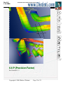
Arbitrary Inductance Calculator User’s Manual
By Robert J Distinti M.S. ECE
46 Rutland Ave.
Fairfield Ct 06825.
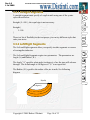
This document details the use of the Arbitrary Inductance (ArbI) calculating software.
This software uses New Electromagnetism to calculate the inductance of inductors. This
software is a limited version of the software developed for my master thesis; see
www.distinti.com/docs/neThesis.pdf.
This software is limited as follows:
1) Copper structures with dimensions no less than 100 microns (0.1 mils).
2) Core materials with μ R = 1, ε R = 1 (same as free space)
3) Low frequency
a. Skin depth larger than max cross section of inductor under test
b. Low frequency inductors (wavelength of highest frequency componenet at least
4 time longer than length of inductor under test: wavelength=c/freq);
Please Read
This software is distributed freely and is intended solely for experimental purposes. This
software is not intended to be used for any other purpose what so ever. www.distinti.com
assumes no liability for the use of this software or the use of the results produced by this
software for any purpose.
Copyright © 2008 Robert J Distinti.
Page 1 of 35
Rev 1.0
1 Jul 2008
The World Leader in Electromagnetic Physics
1 INSTALLATION....................................................................................... 4
1.1 SYSTEM REQUIREMENTS:......................................................................... 4
1.2 INSTALLATION ......................................................................................... 4
2 GETTING STARTED............................................................................... 5
2.1 RUNNING THE SOFTWARE ........................................................................ 5
3 SPECIFYING A SHAPE ........................................................................ 11
3.1 THE SYNTAX OF AN INDUCTANCE SHAPE SPECIFICATION ...................... 11
3.1.1 Comments....................................................................................... 11
3.1.2 Analysis Specification .................................................................... 12
3.1.3 Common Parameters...................................................................... 12
3.1.4 Shape Specification ........................................................................ 12
3.1.5 Shape Specific Parameters ............................................................ 12
3.2 BUILT-IN SHAPES .................................................................................. 12
3.3 ARBITRARY SHAPES .............................................................................. 14
3.3.1 Straight Segments........................................................................... 16
3.3.2 Left/Right Segments........................................................................ 16
3.3.3 Important consideration when using Arbitrary Inductor. ............. 17
4 SAMPLING AND PRECISION SPECIFICATION............................ 18
4.1.1 L and Even/Odd segments.............................................................. 21
4.1.2 Check sample plane spacing for circular segments....................... 23
4.1.3 The Precision Factor P .................................................................. 23
5 GROUND PLANES................................................................................. 26
5.1 SINGLE GROUND PLANES ...................................................................... 26
5.2 DUAL GROUND PLANES ........................................................................ 28
6 PARAMETERS ....................................................................................... 30
6.1 A ........................................................................................................... 30
6.2 B, C, D, N ............................................................................................. 30
6.3 H ........................................................................................................... 30
6.4 HOGP ................................................................................................... 30
6.5 L ........................................................................................................... 31
6.6 P (PRECISION FACTOR).......................................................................... 32
6.7 NGP ...................................................................................................... 33
6.8 NGPI..................................................................................................... 33
6.9 NH ........................................................................................................ 33
6.10 NW ..................................................................................................... 33
6.11 R ......................................................................................................... 33
Copyright © 2008 Robert J Distinti.
Page 2 of 35
Rev 1.0
1 Jul 2008
The World Leader in Electromagnetic Physics
6.12 UP....................................................................................................... 33
6.13 W ........................................................................................................ 34
APPENDIX A. ............................................................................................. 35
Copyright © 2008 Robert J Distinti.
Page 3 of 35
Rev 1.0
1 Jul 2008
The World Leader in Electromagnetic Physics
1 Installation
1.1 System requirements:
1) Microsoft Windows (Me, 2000, Xp, NT) – it should run under Vista.
2) 250Mb Minimum memory (estimated)
3) OpenGL compatible graphics card (most cards are compatible).
1.2 Installation
The installation of this software is very simple. Follow the steps below:
1) Create a new directory on your hard drive (Example c:\arbInd\)
2) Copy the files listed below from the website to your new directory
3) Installation is complete. See next section to run the code.
These are the files:
1) ArbInd.exe (the application)
2) borlndmm.dll
3) cc3270mt.dll
4) dbrtl100.bpl
5) rtl100.bpl
6) vcl100.bpl
7) vclactnband100.bpl
8) vcldb100.bpl
9) vclx100.dll
This software does not affect your Windows installation in any way.
To uninstall the software: simply delete the directory containing the above
files from your computer.
Copyright © 2008 Robert J Distinti.
Page 4 of 35
Rev 1.0
1 Jul 2008
The World Leader in Electromagnetic Physics
2 Getting Started
2.1 Running the software
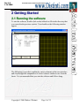
To start the software, double click on the ArbInd.exe file in the directory that
you created in the previous section. You should see the following window
appear.
The following screen-shots explain the various elements of the user interface
and step through the computation of a basic inductor similar to one from the
thesis. It is recommended that you start the software and follow along.
Copyright © 2008 Robert J Distinti.
Page 5 of 35
Rev 1.0
1 Jul 2008
The World Leader in Electromagnetic Physics
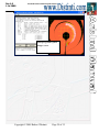
This is the input window
where you specify the
inductor that you would like
to compute. It comes up with
a default inductor
specification.
Copyright © 2008 Robert J Distinti.
Page 6 of 35
Rev 1.0
1 Jul 2008
The World Leader in Electromagnetic Physics
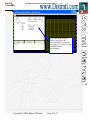
The Open button allows you to
load the input window from a
“notepad” compatible text file.
For this introduction we are not
going to use the Open button.
This is the text output window. This
will show the inductance results in
henries or it will display any syntax
errors found in the input
Copyright © 2008 Robert J Distinti.
Page 7 of 35
Rev 1.0
1 Jul 2008
The World Leader in Electromagnetic Physics
This is the graphic output window.
It is presently empty, showing only
a 50 mil grid pattern (the yellow
lines).
The grid pattern is there to give
you a size reference.
When you are done specifying (or
changing) your inductor, you must
then click the “parse” button for
the software to read your
specification and construct it in the
virtual world.
Click the Parse Input button now.
The min and max dimension (in mils) are displayed
for your reference.
Copyright © 2008 Robert J Distinti.
Page 8 of 35
Rev 1.0
1 Jul 2008
The World Leader in Electromagnetic Physics
The drawing coordinates are shown at
right.
Note: the yellow grid pattern extends only
two inches around the origin (0,0,0)
Y
X
Z
The origin is here.
All inductors begin from the origin.
All inductors (except spirals) begin
drawing toward negative Z.
Clicking the compute button sets
the computation in motion and
returns the inductance in the output
window. The M-field map is also
computed and displayed in the
graphic output.
Copyright © 2008 Robert J Distinti.
Page 9 of 35
Rev 1.0
1 Jul 2008
The World Leader in Electromagnetic Physics
The default inductor results in 269nH. This inductor is experiment #1 from
the thesis.
The next sections details the different ways that an inductor can be specified.
Copyright © 2008 Robert J Distinti.
Page 10 of 35
Rev 1.0
1 Jul 2008
The World Leader in Electromagnetic Physics
3 Specifying a shape
3.1 The Syntax of an Inductance shape
specification
The input window is the place to specify the inductor shape to be tested.
The text in the input window is parsed by simple text parser that reads the
specification and constructs an inductor. You may find it easier to edit these
specifications in notepad or some other ANSI compatible text editor. Then
cut-and-paste them into the input widow, or open the .txt file using the open
button described previously.
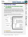
The following diagram details the different sections of an inductor
specification. These sections are described in more detail in the following
paragraphs.
Comments
Analysis
Specification
Common
Parameters
Shape Specification
Shape Specific
Parameters
; Standard inductor shape specification (no Gr
; All dimensions in mils (1000ths of inch)
; see page 58 of thesis for detailed description
inductance_LF{
H 1.35
;Height = copper thickness (mi
W 50
;Width = trace width (mils)
NH 3
;Number of Sample points acro
NW 5 ;Number of sample points across
L 30
; Distance between sample plan
P 2.7
; Precision factor (%) --do not
shape rectangle{
A 2600
; A Dimension
B 3300
; B Dimension
C 600
; C Dimension
D 200
; D Dimension
N3
; Number of turn
} ; This closes the shape specification
} ;This closes the inductance specification
33..11..11 C
Coom
mm
meennttss
All text following a semicolon (;) to the end of a line is ignored by the text
parser. This allows the insertion of comments for human understanding.
Copyright © 2008 Robert J Distinti.
Page 11 of 35
Rev 1.0
1 Jul 2008
The World Leader in Electromagnetic Physics
33..11..22 A
Annaallyyssiiss S
Sppeecciiffiiccaattiioonn
The only analysis specification that the software presently recognizes is
inductance_LF. This stands for low frequency inductance analysis. This
line is required.
33..11..33 C
Coom
mm
moonn P
Paarraam
meetteerrss
The common parameters are independent of the shape of the inductor and
typically control the numerical integration and other features. These
parameters are described in more detail in section 6.
33..11..44 S
Shhaappee S
Sppeecciiffiiccaattiioonn
The Shape specification section defines the inductor shape. There are 4
built-in shapes (Rectangle, circle, spiral and cspiral (corner lead spiral));
these shapes match those used in my graduate thesis.
There is also an arbitrary shape specification which allows an arbitrary shape
to be specified (presently the arbitrary shapes must have same trace width
and height through out.)
The shapes are covered in more detail in the sections that follows.
33..11..55 S
Shhaappee S
Sppeecciiffiicc P
Paarraam
meetteerrss
These parameters are specific to the shape specified. The parameters are
described in the section that follows.
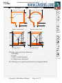
3.2 Built-in Shapes
The 4 built inductors shapes are shown in the following diagram
Copyright © 2008 Robert J Distinti.
Page 12 of 35
Rev 1.0
1 Jul 2008
The World Leader in Electromagnetic Physics
Rectangle
Circle
A
A
H=Copper Thickness
H=Copper Thickness
B
W
W
D
D
C
C
Spiral: Center-lead
Spiral: Corner-lead
W
B
W
B
C
C
C
C
A
H=Copper Thickness
N=Number of turns
A
H=Copper Thickness
N=Number of turns
The shape codes used in the software are
1) Rectangle
2) Circle
3) Spiral (center lead spiral)
4) CSpiral (corner lead spiral)
The following is an example specification for a rectangular inductor.
Copyright © 2008 Robert J Distinti.
Page 13 of 35
Rev 1.0
1 Jul 2008
The World Leader in Electromagnetic Physics
; Standard inductor shape specification (no Ground plane)
; All dimensions in mils (1000ths of inch)
inductance_LF{
H 1.35 ;Height = copper thickness (mils) – 1oz=1.35 2oz=2.7
W 50
;Width = trace width (mils)
NH 3
;Number of Sample points across the height
NW 5
;Number of sample points across the width
L 30
; Distance between sample planes (cuts)
P 2.7
; Precision factor (%) --do not make greater than 2.7
shape rectangle{
A 2600
; A Dimension
B 3300
; B Dimension
C 600
; C Dimension
D 200
; D Dimension
N3
; Number of turns (Spirals only)
}
}
Most of the parameters shows above are self-explanatory; for full details see
section 6.
You can cut-and-paste the above text into the input window. You can
change the inductor shape by replacing the word “Rectangle” with the
appropriate shape code listed above.
3.3 Arbitrary Shapes
This software also allows the specification of an arbitrary shape. The shape
code used for an arbitrary inductor is “Arbitrary”. Inside the brackets (see
example below) list as many “Straight”, “Left” or “Right” segments as
desired (the total number of segments must be an odd number for best
results).
Copyright © 2008 Robert J Distinti.
Page 14 of 35
Rev 1.0
1 Jul 2008
The World Leader in Electromagnetic Physics
; Arbitrary inductor shape specification
; All dimensions in mils (1000ths of inch)
inductance_LF{
H 1.35 ;Height = copper thickness (mils) – 1oz=1.35 2oz=2.7
W 50
;Width = trace width (mils)
NH 3
;Number of Sample points across the height
NW 5
;Number of sample points across the width
L 30
; Distance between sample planes (cuts)
P 2.7
; Precision factor (%) --do not make greater than 2.7
shape Arbitrary{
straight{L 200} ; A straight Section of 200 mils
left{}
; a 90 degree Left turn of radius W*0.51
right{}
; a 90 degree Right turns
Straight{L 50} ; A straight section of 50 mils length
Right{A 45 R 200} ; A right turn of 45 degrees with radius 200 mils
}
}
Copyright © 2008 Robert J Distinti.
Page 15 of 35
Rev 1.0
1 Jul 2008
The World Leader in Electromagnetic Physics
33..33..11 S
Sttrraaiigghhtt S
Seeggm
meennttss
A straight segment must specify a Length in mils using one of the syntax
styles shown below.
Straight {L=100} ; the equal sign is not necessary
Straight {
L 100
}
There is a lot of flexibility in the text parser; you can try different styles that
suite your tastes.
33..33..22 LLeefftt//R
Riigghhtt S
Seeggm
meennttss
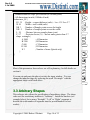
The Left and Right segments allow you specify circular segments or corners
of rectangular inductors.
The Left and Right Segments require two parameters. The parameters are
Angle (A) and Radius ( R ).
The Angle “A” specifies what angle (in degrees) of arc the turn will advance
through. The default angle is 90 degrees is “A” is not specified.
The Radius ( R ) specifies the radius of the arc in mils. See following
diagram.
R(mils)
A (degrees)
Copyright © 2008 Robert J Distinti.
Page 16 of 35
Rev 1.0
1 Jul 2008
The World Leader in Electromagnetic Physics
R specifies the Radius to the centerline of the trace (W/2). R defaults to
W*0.51 if not specified. The software will not let you set R to less than
W/2.
The length of the arc is found with the following equation
L(arc) =
πRA
180
(Length through centerline of arc)
33..33..33 IIm
mppoorrttaanntt ccoonnssiiddeerraattiioonn w
whheenn uussiinngg
A
Arrbbiittrraarryy IInndduuccttoorr..
The number of segments should always be odd. The reason for this is found
in section 4.1.1.
Copyright © 2008 Robert J Distinti.
Page 17 of 35
Rev 1.0
1 Jul 2008
The World Leader in Electromagnetic Physics
4 Sampling and Precision
Specification
The sampling specification consists of 3 parameters (NW, NH and L) and
the Precision specification consists of 1 parameter (P).
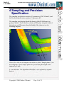
The sampling specification details the density of the M-field map (see
graduate thesis). The M-field is evaluate at NW points along the width of
the inductor and NH points along the height of the inductor (see the
following diagram)
NW=5
NH=3
L
These NW x NH sets of samples form what are called “Sample planes” (see
next diagram). These sample planes are spaced along the length of the
inductor by L mils.
L is not absolute. The algorithm will adjust L on a segment by segment
basis to
Copyright © 2008 Robert J Distinti.
Page 18 of 35
Rev 1.0
1 Jul 2008
The World Leader in Electromagnetic Physics
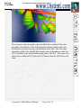
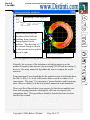
The red arrows show the points where the M-field is evaluated. The color
map shows the intensity of the field (interpolated between the points) and
the direction of red arrows show the direction of the field. The color map
normalizes white to the peak M-field sample point of the inductor under test
(IUT) and black to the min M-field sample point of the IUT. The same color
shown on two different IUT plots does NOT means that the M-Fields are the
same.
Copyright © 2008 Robert J Distinti.
Page 19 of 35
Rev 1.0
1 Jul 2008
The World Leader in Electromagnetic Physics
Beginning of first segment
The red arrows show the
direction of the M-Field
resulting from a current
change applied to the
inductor. The direction of
the current change is shown
by the current source symbol
drawn at right.
End of last segment
Figure 1: The applied current change which results in shown M-Field directions (red-arrows)
Naturally, the accuracy of the inductance calculation improves as the
number of sample points increase (by increasing NW,NH and decreasing L);
however, like many numerical algorithms the time to compute the results
increases.
From experience I have found that for the printed circuits tested in the thesis,
the NW=5, NH=3, L=30 are sufficient to achieve results to within 1% of
convergence. The term “1% convergence” means that the result from using
these values is within 1% of the best possible numerical result obtainable.
There is an Excel Spread sheet (convergence.xls) that shows multiple runs
done with varying parameters detailing the effect on convergence and
computation time. This spreadsheet should be found in the same location
that this file is found.
Copyright © 2008 Robert J Distinti.
Page 20 of 35
Rev 1.0
1 Jul 2008
The World Leader in Electromagnetic Physics
44..11..11 LL aanndd E
Evveenn//O
Odddd sseeggm
meennttss
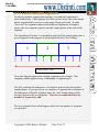
In order to optimize sample plane spacing, even and odd segments are
treated differently. Odd segments (see blue sections below) have the sample
planes (represented by arrows) evenly spaced from end to end. In order
“dove-tail” the segments and prevent inefficient duplication of samples
planes, the even segments (green) omit the sample planes at the ends of the
segment.
The algorithm will reduce L as needed in order to fit the sample planes into a
given segment for the purpose of achieving the desired “dove-tailing.”
1
3
2
Evaluated End To End
Note: this diagram shows three straight segments as an example. This
sampling scheme applies to any combination of segment types.
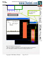
The AIA evaluates the inductance of a structure between the first and last
sample planes. If you specify an even number of segments the evaluation of
the inductance will not be complete since the “end” sample plane will be
missing (shown in the next diagram). Thus it is recommended that the
number of segments be odd.
The next example shows what happens when an even number of segments
are specified.
Copyright © 2008 Robert J Distinti.
Page 21 of 35
Rev 1.0
1 Jul 2008
The World Leader in Electromagnetic Physics
This section missing
from inductance
evaluation
Not evaluated to the end
Figure 2: Even Segments cause data truncation
There are a number of techniques to ensure that the number of segments is
odd. The simplest method is to divide an existing segment in two.
Copyright © 2008 Robert J Distinti.
Page 22 of 35
Rev 1.0
1 Jul 2008
The World Leader in Electromagnetic Physics
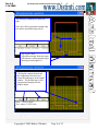
44..11..22 C
Chheecckk ssaam
mppllee ppllaannee ssppaacciinngg ffoorr cciirrccuullaarr
sseeggm
meennttss
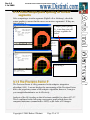
After computing a circular segments (Right/Left or Arbitrary); check the
output graphic to ensure that the curves are not too segmented. If they are,
then decrease L.
If sample plane spacing
(L) is too long you will
get large segments for
circles
Decreasing L
44..11..33 TThhee P
Prreecciissiioonn FFaaccttoorr P
P
The Precision Factor is a key parameter for the adaptive integration
algorithm (AIA). I can not divulge the true meaning of the Precision Factor
due to the proprietary nature of the adaptive algorithm; however, I can give
you enough information to use it effectively.
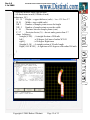
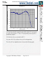
Analysis of the AIA teaches us that it becomes unstable for values of P>2.7.
This is confirmed in the following convergence graph which shows the
computed inductance (normalized to 100%) as the value of P changes.
Copyright © 2008 Robert J Distinti.
Page 23 of 35
Rev 1.0
1 Jul 2008
The World Leader in Electromagnetic Physics
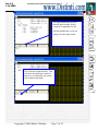
Convergence vs. P
100.2
Computed Inductance (normalized to 100%)
100.1
100
99.9
99.8
99.7
99.6
99.5
99.4
99.3
99.2
0
0.5
1
1.5
2
2.5
3
3.5
P (Precision factor)
The chart shows that the computed results will be within 0.1% convergence
for values of P less than 2.6. Above 2.7 the algorithm quickly degrades as
predicted by analysis.
All of the thesis data was calculated with P=1.
The value of P=2.45 is sufficient for any real world application.
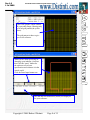
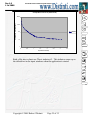
The effect of P on computation time is shown in the following graph.
Copyright © 2008 Robert J Distinti.
Page 24 of 35
Rev 1.0
1 Jul 2008
The World Leader in Electromagnetic Physics
Compuation Time Vs. P (inductor #1)
Computation Time (Seconds)
10000
1000
Series1
100
10
1
0
0.5
1
1.5
2
2.5
3
3.5
P (Precision Factor)
Both of the above charts use Thesis inductor #1. This inductor comes up as
the default test in the input windows when the application is started.
Copyright © 2008 Robert J Distinti.
Page 25 of 35
Rev 1.0
1 Jul 2008
The World Leader in Electromagnetic Physics
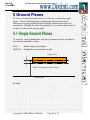
5 Ground Planes
PC traces are typically layered next to, or between, conducting copper
planes. These conducting planes significantly affect the measured
inductance (see my graduate thesis for details) and therefore need to be
considered. Although the term “Ground plane” is used, these planes do not
need to be connected to any potential.
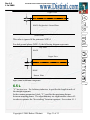
5.1 Single Ground Planes
To specify a single ground plane, only two parameters need to be added to
the common parameter section.
NGP 1
; Enable single ground plane
HOGP 65 ; Height above ground plane in mils
Copper Trace
H/2
HOGP= Height above Ground Plane
Ground Plane
Example
Copyright © 2008 Robert J Distinti.
Page 26 of 35
Rev 1.0
1 Jul 2008
The World Leader in Electromagnetic Physics
; Standard inductor shape specification
; All dimensions in mils (1000ths of inch)
; see page 58 of thesis for detailed description
inductance_LF{
H 1.35 ;Height = copper thickness (mils) - 1oz=1.35 2oz=2.7
W 50
;Width = trace width (mils)
NH 3
;Number of Sample points across the height
NW 5
;Number of sample points across the width
L 30
; Distance between sample planes (cuts)
P 2.7
; Precision factor (%) --do not make greater than 2.7
NGP 1
; Enable single ground plane
HOGP 65 ; Height above ground plane in mils
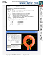
shape circle{
A 260
; A Dimension
B 330
; B Dimension
C 60
; C Dimension
D 100
; D Dimension
}
}
The ground plane
image is seen below
the grid pattern.
Copyright © 2008 Robert J Distinti.
Page 27 of 35
Rev 1.0
1 Jul 2008
The World Leader in Electromagnetic Physics
5.2 Dual Ground Planes
To specify a dual ground plane, three parameters need to be added to the
common parameters section of the specification. These are:
NGP 2
; Enable dual ground plane
HOGP 65 ; Height above ground plane in mils
NGPI 10 ; Number of Ground plane image pairs
If NGPI is not specified, it defaults to 70 image pairs. For description of the
meaning of “number of ground plane images pairs”, see my graduate thesis.
Note: NGPI is only meaningful if NGP = 2; it is ignored for other values of
NGP.
; Standard inductor shape specification
; All dimensions in mils (1000ths of inch)
; see page 58 of thesis for detailed description
inductance_LF{
H 1.35 ;Height = copper thickness (mils) - 1oz=1.35 2oz=2.7
W 50
;Width = trace width (mils)
NH 3 ;Number of Sample points across the height
NW 5 ;Number of sample points across the width
L 30 ; Distance between sample planes (cuts)
P 2.7 ; Precision factor (%) --do not make greater than 2.7
NGP 2 ; Enable dual ground plane
NGPI 4 ;limit to 4 image pairs (70 is default)
HOGP 65 ; Height above ground plane in mils
shape circle{
A 260
; A Dimension
B 330
; B Dimension
C 60
; C Dimension
D 100
; D Dimension
}
}
Copyright © 2008 Robert J Distinti.
Page 28 of 35
Rev 1.0
1 Jul 2008
The World Leader in Electromagnetic Physics
Multiple ground plane
images seen.
Copyright © 2008 Robert J Distinti.
Page 29 of 35
Rev 1.0
1 Jul 2008
The World Leader in Electromagnetic Physics
6 Parameters
This section gives detailed description of the parameters used to specify an
inductor.
6.1 A
The parameters A is used differently depending upon the shape selected.
For “built-in” shapes, “A” represents dimension A of the “Built-in” shapes.
See section 3.2 for a list of the built in shapes.
For Arbitrary Shapes, “A” represents the angle (in degrees) through which a
“Right turn” or “Left turn” will progress (see section 3.3.2)
6.2 B, C, D, N
These are “Built-in” shape specific parameters. Please see section 3.2 for
their meaning.
6.3 H
H is the trace height in mils. Use 1.35 for 1oz copper and 2.7 for 2 oz
copper.
6.4 HOGP
HOGP is height above ground plane. This is the distance from the surface of
the ground plane to the centerline of the trace.
Copyright © 2008 Robert J Distinti.
Page 30 of 35
Rev 1.0
1 Jul 2008
The World Leader in Electromagnetic Physics
Copper Trace
H/2
HOGP= Height above Ground Plane
Ground Plane
This value is ignored if the parameter NGP=0
For dual ground planes (NGP=2), the following diagram represents
Top Plane
HOGP
Copper Trace
H/2
HOGP
Bottom Plane
Figure 3: Dual Ground Plane configuration
6.5 L
“L” has two uses. For Arbitrary inductors, it specifies the length in mils of
the straight segments.
In the common parameters block, “L” specifies the maximum distance
between sampling planes. The algorithm may use slight smaller values of L
in order to optimize the “dove-tailing” between segments. See section 4.1.1
Copyright © 2008 Robert J Distinti.
Page 31 of 35
Rev 1.0
1 Jul 2008
The World Leader in Electromagnetic Physics
NW=5
NH=3
L
6.6 P (Precision Factor)
See Section 4.1.3
Copyright © 2008 Robert J Distinti.
Page 32 of 35
Rev 1.0
1 Jul 2008
The World Leader in Electromagnetic Physics
6.7 NGP
Number of ground planes.
NGP=0 for no ground planes
NGP=1 for single ground planes
NGP>=2 for Dual Ground planes
6.8 NGPI
Number of Ground Plane Image Pairs. When considering dual ground
planes (NGP=2) the precision of the results depends upon the number of
ground plane images that are processed. See graduate theses for more
details.
The computation time for dual conducting planes is based on the number of
image reflection that the user desires. The number of images that require
volume integration is 1+NGPI*2. The adaptive algorithm processes these
reflected images very quickly.
6.9 NH
The number of sample points along the height of the inductor.
6.10 NW
The number of sample points across the width of the inductor.
6.11 R
The radius of left or right turns in mils. Defaults W*0.51 which gives very
tight turns.
6.12 UP
An optional parameter in a “Left”, “Right” or “Straight” segment of an
arbitrary inductor specification. To be used to route traces up/down to create
Copyright © 2008 Robert J Distinti.
Page 33 of 35
Rev 1.0
1 Jul 2008
The World Leader in Electromagnetic Physics
helixes or to pass traces over one another. Defaults to 0. Do not use, has not
been tested yet.
6.13 W
Width of the inductor trace in mils.
Copyright © 2008 Robert J Distinti.
Page 34 of 35
Rev 1.0
1 Jul 2008
The World Leader in Electromagnetic Physics
A
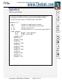
Appppeennddiixx A
A..
Inductor specifications
; This uses the arbitrary inductor to specify experimental inductor #1
; The purpose of this is to test to ensure that the Arbitrary shape
; can give the same value as a built in shape. And it does
;
inductance_LF{
NH 3
; Number of sample points in height
NW 5
; Number of sample points across width
L 30
; Distance between cuts
P 2.45
; Precision factor (%) --do not make greater than 2.7
shape arbitrary{
H 1.35 ;Height = copper thickness
W 50
;Width = trace width
straight{L=150}
right{R=50}
straight{L=900}
left{R=50}
straight{L=3200}
left{R=50}
straight{L=2500}
left{R=50}
straight{L=3200}
left{R=50}
straight{L=900}
right{R=50}
straight{L=150}
}
}
Copyright © 2008 Robert J Distinti.
Page 35 of 35