Download FPS-ATLAS Tutorial - Connect - University of British Columbia

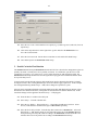
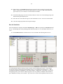
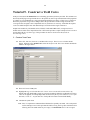
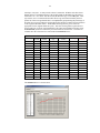
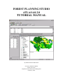
1
FOREST PLANNING STUDIO
ATLAS 6.0.2.0
TUTORIAL MANUAL
By: Mark Perdue and John Nelson
University of British Columbia
Faculty of Forestry
Department of Forest Resources Management
February 4, 2009
2
TABLE OF CONTENTS
TABLE OF CONTENTS ............................................................................................................................. 2
INTRODUCTION ........................................................................................................................................ 4
DOWNLOADING FPS-ATLAS FROM THE FRST 424 WEB PAGE (RECOMMENDED)..................................... 4
DOWNLOADING FPS-ATLAS FROM THE FTP SITE ..................................................................................... 5
STARTING ATLAS-FPS ON THE UBC FORESTRY LAB COMPUTERS ........................................................... 5
TUTORIAL 1. OPEN A DATABASE FOR WORK WITH FPS............................................................ 7
1. CREATE A WORKING FILE ................................................................................................................... 7
OPEN FOREST PLANNING STUDIO................................................................................................................ 7
LOAD AN EXISTING FPS DATABASE............................................................................................................ 8
TUTORIAL 2. HARVEST SIMULATION ............................................................................................. 11
2. SCHEDULE HARVEST FLOW ............................................................................................................... 11
2. MODULE CONFIGURATION ................................................................................................................ 13
3. APPLY A TREATMENT ........................................................................................................................ 14
4. INITIATE A RUN ................................................................................................................................. 15
5. FIND THE MAXIMUM HARVEST VOLUME .......................................................................................... 19
TUTORIAL 2 SUPPLEMENTAL (LINKING ESTIMATES OF LTSY AND EXTREME DEPARTURES TO FPS RUNS)
.................................................................................................................................................................. 21
TUTORIAL 3. CONSTRAINTS AND HARVEST PARAMETERS .................................................... 24
6. CREATE A CONSTRAINT SET (CSET).................................................................................................... 24
2. APPLY THE NO HARVEST CSET ......................................................................................................... 25
3. DEFINE THE RESERVE ZONE SPATIALLY ............................................................................................ 26
4. RUN THE SIMULATION ....................................................................................................................... 28
EDIT THE COLOUR PALETTE ...................................................................................................................... 29
TUTORIAL 4. APPLY AN ADJACENCY CONSTRAINT................................................................... 31
1. CREATE AN ADJACENCY CONSTRAINT .............................................................................................. 31
RUN THE SIMULATION ............................................................................................................................... 32
TUTORIAL 5. SCHEDULE WITH SORTS............................................................................................ 34
1. SELECT THE RESERVE & ADJACENCY RULE SET ............................................................................... 34
CLOSE THE BROWSER................................................................................................................................ 34
RESET THE DEFAULT SORT ....................................................................................................................... 34
RUN THE SIMULATION ............................................................................................................................... 34
2. RANDOM HARVEST PRIORITY/SORT .................................................................................................. 36
RUN THE SIMULATION ............................................................................................................................... 36
TUTORIAL 6. SCHEDULE LONG ROTATIONS ................................................................................ 37
1. LONG ROTATIONS ............................................................................................................................. 37
RUN THE SIMULATION ............................................................................................................................... 38
TUTORIAL 7. SET MINIMUM LEVELS OF OLD FOREST.............................................................. 39
APPLY THE CSET ....................................................................................................................................... 40
RUN THE SIMULATION ............................................................................................................................... 40
TUTORIAL 8. SCHEDULE PARTIAL CUT HARVESTS .................................................................. 43
1.
2.
CREATE A PARTIAL CUT STAND GROUP ............................................................................................ 43
PARTIAL CUT IN THE FIRST ROTATION .............................................................................................. 45
3
RUN THE SIMULATION ............................................................................................................................... 46
TUTORIAL 9. CONSTRUCT A YIELD CURVE ................................................................................. 48
1. CREATE A NEW CURVE ..................................................................................................................... 48
RUN THE SIMULATION ............................................................................................................................... 53
TUTORIAL 10. EDIT INDIVIDUAL POLYGONS .............................................................................. 54
1. QUERY THE DATABASE ..................................................................................................................... 54
EDIT POLYGON .......................................................................................................................................... 54
TUTORIAL 11 EDIT BY FENCING POLYGONS................................................................................ 56
1. QUERY THE DATABASE ..................................................................................................................... 56
FENCE THE QUERIED POLYGONS ................................................................................................................ 56
TUTORIAL 12 APPLY COMMERCIAL THINNING .......................................................................... 58
1. CREATE A VOLUME-AGE CURVE FOR THINNED FIR STANDS ......................................................... 58
2. CREATE TWO NEW STAND GROUPS .................................................................................................... 58
IDENTIFY STANDS ELIGIBLE FOR COMMERCIAL THINNING ....................................................................... 59
FREQUENTLY ASKED QUESTIONS ................................................................................................... 64
4
INTRODUCTION
This manual provides some basic examples of the FOREST PLANNING STUDIO (FPS) – ATLAS
PROGRAM. These tutorials are nested and hierarchical so that the each tutorial prepares the user for the
next. More specific and detailed explanations of FPS are available in the FPS-ATLAS manual. The
manual and the FPS program are available at no cost on the FRST 424 web site or the ATLAS FTP site.
Downloading FPS-ATLAS from the FRST 424 Web Page (Recommended)
1.1. System Requirements
FPS requires the following software (check your versions) and system specifications.
Windows 2000, Windows XP
Microsoft Access 2000 or later
1.2. Connect to the FRST 424 web site at UBC http://courses.forestry.ubc.ca/frst424 Choose the
Modelling tab and select ATLAS Model Documentation & Tutorials.
1.3. Under the heading FPS-ATLAS FILES, download “FPS-ATLAS Install Program Files (Zipped)”
to a temporary folder (e.g D:\tmp). This downloads a file named Giz_May_06.zip. WARNING:
DO NOT PLACE THE FILE WAY DOWN IN THE FOLDER STRUCTURE (e.g. C:\my
stuff\junk\morejunk\junkagain\...\etc.
1.4. Unzip this file using the unzip to folder option and you will get the following structure:
1.5. Open the Install_Version folder and run Setup.exe to install FPS. It will install the program in
the folder Program Files\Forest Planning Studio, and a subfolder called Components.
1.6. Now move to the Update_Version folder. Copy the files in the subfolders (Components and
Forest Planning Studio) and overwrite the files in the corresponding folders found in Program
Files\Forest Planning Studio, and the subfolder Components.
1.7. From the FRST 424 web site, download FPS-ATLAS Tutorial Database (Gavin 2009) to a
working folder on your hard drive. This downloads the file Gavin_2009.zip. Unzip this file and
you have Gavin_2009.mdb. You can now open this file with FPS.
5
Downloading FPS-ATLAS from the FTP Site
1.8. System Requirements
FPS requires the following software (check your versions) and system specifications.
Windows 2000, Windows XP
Microsoft Access 2000 or later
1.9. Connect to the UBC FTP Site using FTP software such as WS_FTP (this software can be found on
the web at www.ipswitch.com).
atlas.forestry.ubc.ca
Login as atlas1
Password=atlas-1
Directory = Atlas\ATLAS-PROGRAM\FPS_Program\Version_6\
1.10. Copy the files in the Install_Version folder to temporary folder on your hard drive. WARNING:
DO NOT PLACE THE FILE WAY DOWN IN THE FOLDER STRUCTURE (e.g. C:\my
stuff\junk\morejunk\junkagain\...\etc. Within the Install_Version folder, run Setup.exe to install
FPS. It will install the program in the folder Program Files\Forest Planning Studio, and a
subfolder called Components.
1.11. From the FTP site, copy the files in the folder Update_Version to a temporary folder on your hard
drive. Now copy these files to overwrite the files in the folders Program Files\Forest Planning
Studio, and the subfolder Components.
1.12. From the FTP copy Atlas\ATLAS-PROGRAM\FPS_Program\tutorials\Gavin_2009.zip to a
working folder on your hard drive. Unzip this file and you have Gavin_2009.mdb. You can now
open this file with FPS.
Starting ATLAS-FPS on the UBC Forestry Lab Computers
You need to move a few files and set some defaults before running ATLAS-FPS on the computers in the
forestry labs. The file Gavin_2009.mdb is a MSAccess database for the Gavin Block of the AFRF and is
used in the training tutorials. The file Palette.mdb is an MS Access database file that controls viewing
options (map colours and legends).
1.
On your User drive, create a folder called “atlas”, and under “atlas” create another folder called
“runs” (e.g. U:\atlas\runs)
2.
Copy the file “Gavin_2008.zip” from the FRST 424 web page (Modelling\Atlas Model
Documentation & Tutorials) to U:\atlas (the file is zipped, so unzip it when downloaded =
Gavin_2009.mdb)
3.
Copy the file Palette.mdb from the FRST 424 web page (Modelling\Atlas Model Documentation
& Tutorials) to U:\atlas (the file is zipped, so unzip it when downloaded)
4.
Start FPS (it’s under the Forestry Applications menu as Forest Planning Studio). Under tools,
choose palette location. Select the file Palette.mdb in U:\atlas. Close the program and then restart it. FPS will now use this palette file each time it is opened (you will have do this the first
time you run it on a different computer in the labs).
6
5.
You will also need to set a default directory in the run window (U:\atlas\runs) so that you don’t fill
your U: drive with megabytes of output files. You will be given instructions on this in the
tutorials that follow.
The file containing the tutorials is on the FRST 424 web page modelling\Atlas Model Documentation &
Tutorials\Documents\FPS-ATLAS Tutorials 2009. There are 12 tutorials that you can progress through at
your own pace.
There is also a program manual (ATLAS User Manual) in the same place that has detailed program
information and formulation examples. I have printed 1-2 copies that I will leave in the class room.
Finally, the web site www.forestry.ubc.ca\atlas-simfor has quite a few extension reports on the model and
its application to various planning problems.
7
Tutorial 1. Open a Database for Work with FPS
1. Create a Working File
FPS automatically saves changes to the mdb file as you work. The advantage of this design is that current
edits are never lost, the disadvantage is that the original file is not retained. It is therefore prudent to
create a working file from the original file.
1.1. In Windows Explorer create a folder named ATLAS to save your FPS work (FSC students should
create this folder on their U drive as described in the Introduction). Save the file
Gavin_2009.mdb as a backup. To create a working file, make a copy of Gavin_2009.mdb and
rename it GavinTut.mdb.
1.2. To backup your work at the end of each tutorial, zip working file (e.g. GavinTut.zip). You can
continue working on GavinTut.mdb, but if for some reason you need a backup, just unzip
GavinTut.zip.
Open Forest Planning Studio
2.1. You will likely need to create a shortcut on your desktop to FPS.exe that is located in
C:\Program Files\Forest Planning Studio. Once the shortcut is established, double click on the
shortcut to open the FPS program.
2.2. The FPS window should appear as shown below.
File Folder
8
Load an Existing FPS Database
3.1. Click on the File menu and select Open. Browse for the file GavinTut.mdb and open it. You
will not have all the files shown below, but you will have GavinTut.mdb.
3.2. Below is a description of the FPS toolbar icons. These toolbars are used regularly so it is
helpful to become familiar with the icon names and functions.
Run icon
Configuration Editor
Toggle Browser
New View
Rule Set Editor
Zoom In
Pan
Fit
Zoom Out
Fence
Period Selector
9
3.3. Managing the Rule Set, Browser and Configuration windows. You will find three windows
open. The default locations of these windows are: Browser and RuleSet on the right side and the
Configuration at the bottom. You can move these windows to wherever you like. We suggest
that you dock the RuleSet window on the left side, dock Browser at the top and leave the
Configuration window docked at the bottom, as shown below. To dock these windows, just drag
and drop to the appropriate location. You should only have these windows open when you
need them. Do not maximize these windows and use the FPS Toolbar icons to open and
close them as needed. Maximizing the windows will tend to cover up other windows that
you have neglected to close, resulting in a mess.
3.4. Close the Browser, RuleSet and Configuration windows using the FPS Toolbar icons.
3.5. To view the map of this database, click on the New Viewer icon. Do not maximize the Viewer
window. Maximizing the window will tend to cover up other windows that you have
neglected to close, resulting in a mess that will come back to bite you. Always close the
Viewer window when it is not needed. The information presented in the Viewer depends on the
Viewer settings from the previous FPS session. The current settings are indicated by checkmarks
in the Viewer Control that is located on the left of the viewer window.
In the Viewer Control, click on the box adjacent to the Polygon topology view. Expand the
Polygon topology view by clicking the + to the left of the checkmark. Continue to select, by
clicking in the radio buttons, and expand to the Attribute and Age categories. The Map Viewer
should display the age-class of each polygon and the Palette file is used to display the age-class
legend.
Explore some other views available in the Viewer. Note that this particular database does not
have roads, superblocks, raster cells or streams defined. Close the Viewer by clicking the X at the
top right corner of the Viewer.
10
Viewer control
Close viewer
11
Tutorial 2. Harvest Simulation
FPS simulates spatially explicit harvest scenarios based on target harvest levels & harvest priorities (found
in the Flow & Parameters tab in the RuleSet window) and user-defined harvest constraints (CSets found in
the Browser window). This tutorial describes the first of these two basic procedures, i.e. Flow &
Parameters.
2. Schedule Harvest Flow
1.1. Open the Rule Set Editor. The Rule Set window should appear as shown below. Rule Sets
contain user-defined harvest flow targets and run parameters such as harvest priorities for age or
distance and switches for Superblocks. It also provides an interface to set criteria for edge and
interior forest calculations. Different Rule Sets can be created and saved. Each Rule Set is
tabbed. In the figure below only the default Rule Set is shown.
1.2. Create a new Rule Set. Right-click with the mouse inside the Rule Set window, select New Rule
Set from the dropdown menu. The Forest Planning Studio – Create New Record window should
appear as below. Enter the name Crash in the Description and Abbrev boxes. Select OK to save
the new Rule Set
12
1.3. Ensure that the Crash tab is selected. Select the Flow tab from the Rule Set window. Highlight
the Year or Flow box within the Flow window with the mouse. While the box is highlighted,
depress the Ctrl + Down-arrow to create a row. Enter the Year 10 and a Flow of 200,000 m3,
This value represents the total volume cut within that planning period (e.g. 10 years). In
FPS this periodic harvest volume is all cut in the specified year (10).
1.4. With the cursor in the Rule Set window click the right mouse button. Select the Configure
Flows…, the Configure Planning Horizon window should appear (shown below). Enter a Time
Increment of 10 (if not already displayed), a Final Year of 240 and Use last value to fill in the
Flow of 200,000 m3. The Year and Flow should now be filled in for the entire planning horizon.
1.5. Select the Parameters (Param) tab. Set the Default Sort to 1-Age and the Default Extra Sort to
0-none (always check the sort setting after creating a new Rule Set). The other boxes should be
unmarked, the Edge Contrast as 6-old scraps, 1-regen/shrub and the Edge Depth to 100m.
These setting are shown below. Check that the remaining windows (i.e. Zone, AUnit, Range,
Edge) are empty. The AgeClass tab will have some values in it and these should remain as they
are.
1.6. Close the Rule Set window by toggling it off with the FPS icon or clicking in the top right hand
corner.
13
2. Module Configuration
The Configuration window contains the modules that will be run during each planning period. There are
numerous modules that can be added, but they also affect FPS computing time, therefore include only those
modules necessary.
2.1. Edit the configuration
2.1.1. Select the Configuration Editor icon. The default Configuration window should be similar
to that shown below.
2.1.2.
The checkmarks indicate modules that are active. To activate or deactivate a module, left
click in the box to the left of the module name. These changes are automatically saved.
2.2. Create a new configuration
2.2.1.
Locate the mouse pointer within the Configuration window, right click and select New
Configuration from the drop-down menu.
2.2.2.
Enter Minimum in the Description and Abbreviation (Abbrev) windows. Select OK. The
Minimum configuration should appear as a tab in the Configuration window.
2.2.3.
Locate the mouse pointer within the Minimum configuration window and then right click.
From the drop-down menu select Append. The Select FPS Components to add to the
current configuration window should appear as below.
14
Highlight the Scheduler_V6000 component with the left button of the mouse. Select OK. The
Scheduler_V6000 should now be displayed in the Minimum configuration window. Repeat step
2.2.4 to include Report Ages, Report Areas, Report Volumes and GrowingStock… The
Configuration window should appear as below. You can now close the configuration window.
2.2.4.
3. Apply a Treatment
3.3. Apply Clearcut treatments to Stand Groups 1-FIR, 2-PL/S and 3-Decid.
3.3.1. From the FPS toolbar select the Toggle Browser icon. The Browser window should appear
as shown below. Open the (Stand Group) SGrp tab. Six Stand Groups are listed.
15
3.3.2. Select Stand Group 1 – FIR by double clicking with the left-mouse-button. The Stand
Group 1 – FIR window should appear as below.
3.3.3. Click the Clearcut treatment radio button. Enter Minimum and Maximum values of 50 and
999 respectively. These are the minimum and maximum ages that define when the
treatment is allowed.
3.3.4. Close the Stand Group window by selecting the X in the top right corner. Accept the
changes to Stand Group 1 – FIR. The Stand Group window will be used again in upcoming
tutorials and reviewed in detail in Tutorial 7.
3.3.5. Repeat steps 3.1.2 through 3.1.5 for Stand Group 2 – PL/S and Stand Group 3 – Decid.
Close the Browser window.
4. Initiate a Run
4.1. To initiate a run, click on the Run icon located on the FPS toolbar. The following window should
appear.
16
4.2. Click the Start button. The simulation should have produced a harvest schedule of Flow, Harvest
and Area values similar to those shown below. Notice that the Flow targets are achieved through
the first 18 planning periods (Year 180) but decline rapidly beyond that period. These results
have been automatically saved, in this example in C:\program files\forest planning studio\runs
(U:\ATLAS\runs when running on the FSC computer labs). Unless a default folder for the run
files is created, every run will produce a new folder that can become confusing and waste disk
space. To avoid this do the following.
4.2.2. Change the name from U:\January 18, 00@09-45-… to U:\Atlas\runs
4.2.3. Right click anywhere in the run window and select Save Directory as Default (see Fig.
below). Now, all output files go to this folder, and will overwrite files from previous runs.
This is OK because we can always replicate a previous run.
17
Right click to set
default directory
Note the Growing stock graph in the lower right corner of the Run window. Growing stock is measured as
the total volume, regardless of age (i.e. not merchantable growing stock above the minimum harvest age).
The blue line represents the growing stock in areas that are not eligible for harvest, and it steadily increases
with time as these stands age in the absence of harvesting and natural disturbance. The green line is the
growing stock that is not restricted from harvest and it rapidly declines until near the end of the planning
horizon. This corresponds with the crash in the harvest schedule when there isn’t sufficient timber to
support the 200,000 m3/decade target. The red line is the total of the reserved and non-reserved growing
stocks.
4.3. To view results in more detail, double click on a Year and from the drop-down menu select
Polygon. For each Period of the simulation, you can view the attributes of each polygon. A
portion of this detailed summary table is shown below. Use the Period selector arrows to cycle
through the planning periods and observe how the attributes of each polygon change.
18
4.4. To view these results spatially with the Map Viewer highlight any Year shown in the Run
window, drag and then drop this value into the Map Viewer. The Period Selector should become
activated.
4.4.1. In the Viewer legend, left click on the box adjacent to the Polygon topology view. Expand
the Polygon topology view, continue to select, by left clicking in the circles, and then
expand the Attribute and Age categories. The Map Viewer should display the age-classes of
each polygon while the Viewer Palette should display the age-class legend.
4.4.2. Use the Period Selector to cycle through the planning periods and observe the polygon ages.
You can have the viewer display the current age value of each polygon by expanding the Format tree at the
top of the Viewer Control and selecting Text (See Fig. below).
19
5. Find the Maximum Harvest Volume
In the previous example the Flow targets were not achieved throughout the entire planning horizon. You
will now modify the harvest flows so that the target is met in all periods. There are an infinite number of
ways of doing this, so you need some guidelines. In our case, we want to maximize the early period
harvest and gradually drop down to a long run sustained yield harvest. Further, the drop in harvest from
one period to the next cannot exceed 10%, and the harvest is never to drop below the LRSY.
Create another Rule Set named Conv + LRSY. Note that FPS recognizes this as Rule Set 2. Note that the
parameters set in the old Rule Set are not transferred into the new Rule Set. The desired parameters
must be entered for each new Rule Set.
5.1. In Conv+LRSY, modify the harvest targets according to the table below. The harvest flows
(targets) in this table were derived by trial and error and represent one possible solution to our
scheduling problem.
5.2. Set the harvest priority (sort) to Age
NOTE –harvest targets to the nearest 1000m3 are quire sufficient for this tutorial. In
general, we played with the first 3-5 periods until they worked, then we moved on to the
latter periods. We then had to come back to the earlier periods for some final adjustments.
Year
10
20
30
40
50
60
70
80
90
100
110
120
130
140
150
160
170
180
190
200
210
220
230
240
Flow(m3) Harvest(m3) Area
200,000
201,370
474
195,000
195,815
505
190,000
199,048
523
188,000
188,438
482
186,000
187,776
463
185,000
191,146
495
185,000
190,846
529
185,000
187,986
504
185,000
185,790
496
185,000
186,147
561
185,000
190,441
671
185,000
191,200
686
185,000
191,506
641
185,000
186,805
644
185,000
188,667
672
185,000
189,600
726
185,000
188,482
753
185,000
186,657
826
185,000
189,527
958
185,000
185,553
899
185,000
188,004
927
185,000
187,193
1,043
185,000
185,709
1,204
185,000
185,868
1,624
You should get the results shown in the following figure.
20
Note that the growing stock displays similar trends to the last harvest schedule, but it hasn’t hit rock bottom
(yet).
Question:
What happens if you run the simulation for another 100 years at 185,000 m3/decade (years 240-340 at
185,000 m3/decade?
An alternative harvest schedule following the same objectives (maximize early harvest, maximum 10%
decline and harvest always >= LTSY) is shown in the following Figure. Note that the simulation was run
for 340 years rather than 240 years, and that LTSY is lower over 340 years than it was for the 240 year run.
21
Note that the growing stock first declines rapidly and then declines at a slower rate. Ideally, we would like
the harvest and the growing stock to stabilize in the long-term in order to have more confidence that LRSY
has been reached.
Tutorial 2 Supplemental (Linking Estimates of LTSY and Extreme Departures to
FPS Runs)
This supplemental section links some basic conversion concepts (e.g. LTSY, extreme departures) to harvest
scheduling with FPS.
The Table below shows the area (ha) in the THLB and the N-THLB by age class as determined by an
external query of the database.
AgeCls
THLB
N-THLB
0-20
938.7
434.1
21-40
83.7
61.3
41-60
462.7
0.0
61-80
1,235.7
0.0
81-100
317.4
0.0
101-120
1,670.4
3.5
121-140
503.0
32.8
141-160
30.4
1.6
161-180
85.6
16.3
181-200
46.7
0.0
201-220
125.1
0.0
240+
260.6
0.0
Total
5,760.1
549.6
22
Initial Age-Class
1800
1600
1400
1200
1000
Ha
N-THLB
THLB
800
600
400
200
0
0-20 2140
4160
6180
81- 101- 121- 141- 161- 181- 201- 240+
100 120 140 160 180 200 220
Age-Class
Figure showing the initial age class distribution by the THLB and N-THLB.
A query of the database shows that Stand Groups 1,2,and 3 have 4005, 817 and 938 ha in the THLB,
respectively. If these are to be harvested at age 50 years, the volume/ha cut is 118, 88 and 78 m3/ha,
respectively. Therefore, our estimate of LTSY is 12,353 m3/yr or 123,530 m3/decade.
Estimate of LTSY
StandGroup_Id SumOfArea (ha) m3/ha@ age 50
LTSY m3/yr
1
4,005.3
118
9,453
2
817.2
88
1,438
3
937.6
78
1,463
Total
5,760.1
12,353
Note how close this estimate of LTSY is to that found in the alternate harvest schedule shown at the end of
Tutorial 2 when the planning horizon was extended to 340 years.
Extreme Departure
Another good starting point is to see how the forest behaves at an extreme departure (harvest everything as
soon as it is available). By setting the harvest target higher than that which can ever be cut (e.g. 2,000,000
m3/decade), we can see that a very high harvest is achieved every 50 years (next Figure). Create a new
RuleSet called Max_Departure with these flows and Age as the harvest priority. Because of the initial age
class distribution, there are still some stands that are harvested in between each 50 year peak.
23
Figure showing the extreme departure. Note how the growing stock pattern is the “inverse” of the harvest.
In periods of high harvest, the growing stock rapidly declines and in periods of low harvest, the growing
stock increases rapidity.
At his point, you should have four RuleSet tabs as shown below. If you want to re-run a previous harvest
schedule (RuleSet), just select the appropriate RuleSet and run the model. This is how FPS-ATLAS allows
us to create multiple harvest scenarios within one database (e.g. GavinTut.mdb), and it is the reason we
don’t need to save our output files every time we run the model.
AT THIS POINT YOU SHOULD EXIT FPS AND ZIP YOUR DATABASE (GavinTut.zip). THIS
WILL BE YOUR BACKUP IN CASE YOU MAKE SERIOUS ERRORS IN SUBSEQUENT
TUTORIALS. ZIPPING THE DATABASE AT REGULAR INTERVALS IS YOUR BEST BACKUP METHOD.
24
Tutorial 3. Constraints and Harvest Parameters
(Continue with the database GavinTut.mdb)
To model with FPS it is necessary to define the constraints (CSets) that will affect harvest scheduling. In
Tutorial 2 harvesting was scheduled without constraints, however, in practice there are always numerous
constraints. Often, constraints vary throughout a forest estate and therefore it is necessary to define and
apply a number of different Csets. Further, one of the real values of forest-estate modeling is the
opportunity to observe the consequences of various scenarios. Therefore, a variety of different CSets are
created and applied to each area within the forest estate. This tutorial describes the basic procedures
necessary to define these constraints.
6. Create a Constraint Set (CSet)
A Constraint Set is a collection of management objectives that impose constraints on harvesting. FPS
allows a number of constraints to be identified and applied as a single set; the Constraint Set.
1.1. Select File, then New, then highlight Constraint Set, and then OK to accept the selection. The
New Constraint Set window should appear. Check the Disable Harvesting? box.. In the
Description box type: No Harvest.
1.2. To save the No Harvest constraint set, close the New Constraint Set window and then accept the
changes.
1.3. Select the Toggle Browser button, the Browser window should appear. Select the CSet tab at the
bottom of the Browser window. You will see the No Harvest Cset listed (Fig below). Note:
You may have to click the Exec icon or the press the F5 key to refresh the window.
25
1.4. Now make a new RuleSet called Conv+LTSY+RSV. Copy the harvest flows from the RuleSet
CONV+LTSY and paste them into the new RuleSet CONV+LTSY+RSV. Also set the harvest
priority to Age in the new RuleSet. We are making a new RuleSet that will use the harvest flows
from CONV+LTSY, but it will also be linked to the No Harvest CSet. CSets must be linked to a
RuleSet to be active.
Close the RuleSet window.
2. Apply the No Harvest CSet
2.1. Now that the No Harvest CSet has been defined it is necessary to apply it to a spatial unit (i.e. a
Clique, a Zone, an Access Unit, or a Range.
2.2. This newly created CSet can be applied to an existing Zone or, alternatively, a new Zone can be
created. To create a new Zone, select: File, New, Zone, OK. Type in Reserve Zone and the New
Zone window should appear as in the Figure below. Note that two zones (Zone 1 is the THLB
and Zone 2 is the N-THLB) already exist, so you new Zone is number 3. Close this window and
accept the change.
2.3. In the Browser window, open the Reserve Zone window and select the Constraints tab. In the
Constraints page highlight the Constraints Set box and then simultaneously press the Ctrl +
Down-arrow keys. A drop-down list of CSets, including No Harvest, should appear. Doubleclick on No Harvest to apply this CSet to the Reserve Zone. As a default, this CSet will be
applied for a Duration of 999 years (see Fig. below). Accept the changes.
26
Close the Browser widow.
3. Define the Reserve Zone spatially
3.1. It is always necessary to physically define spatial units. Once the Reserve Zone has been created
it is necessary to add the desired polygons to it.
3.2. In the Viewer’s legend, expand the Polygon topology view by pressing the + beside it, and then
select Zone from this expanded list. Expand the Id to view the Zone legend. Reserve Zone
should be included in this list. If not, select Refresh from the Window caption on the FPS toolbar.
If the Reserve Zone is still not listed the Zone was not properly created.
3.3. Polygons, the basic spatial elements in FPS, can be assigned to Zones by fencing operations,
polygon edits or executing SQL operations. This example will demonstrate the fencing
operation.
27
3.3.1. On the FPS toolbar, press the Fence icon
. The mouse’s pointer can now be used to
“digitize” around polygons (i.e. fence) that you want to select in the Viewer map. As long
as any portion of a polygon is contained within the Fence, it will be selected. Select the
polygons located in the south-west portion of the Gavin Lake map (See Fig below) by left
digitizing the fence. To close the Fence, right click. .
3.2.2. With the pointer located anywhere in the Viewer, right click and select Fence Operation. A
dialog box listing the selected polygons should appear. This list can now be edited,
polygons can be added by typing in the polygon number and selecting Add, polygons can
also be deleted from this list by highlighting the polygon and then depressing the Delete
key. Edit your list so that the only those polygons listed below are included on your list.
28
3.2.3. In the Fence Operation window, the Choose polygon zone value, and select 3 Reserve
Zone. Then click the Apply button and answer yes.
3.2.4. Reserve Zone and its No Harvest CSet are now applied spatially and are visible on the
Map Viewer. In the Viewer Control, select Zone and you will see the new Reserve Zone.
Select the Browser and click on the Zone tab, Reserve Zone should have Constraint Set #1
(No Harvest) applied to Zone
Close the Browser.
4. Run the simulation
4.1. Make sure that you are still in the Conv+LTSY+RSV RuleSet. FPS will now include the No
Harvest Constraint for the Reserve Zone. Click the Run button and you should get the following
harvest schedule.
Open the Viewer and ensure that the polygons in the Reserve Zone are never harvested (they all grow
older).
29
4.2. Now create a new RuleSet called NewFlow+RSV. Be sure to set Age as the harvest priority and
apply the No Harvest CSet to the Reserve Zone (recall that Csets are not automatically
transferred to new RuleSets – they must be manually linked each time a new RuleSet is created).
Then add the flow targets shown in the Figure below (the easiest way to do this is to copy the
flows from the Conv_LTSY+RSV RuleSet and paste them into the new RuleSet). The new
harvest flows have been adjusted downwards to reflect the loss of the THLB caused by the
reserve zone. This was done through trial and error (i.e. iteration) until the harvest flow objectives
were met (transition to new LTSY).
Close the RuleSet window.
Note the growing stock …what happens if you run the simulation for 340 years?
At this point you should have the following RuleSets (i.e. management scenarios) in your model.
Edit the Colour Palette
To edit the colour palette of the Reserve Zone (or any other Zone or legend) click on the colour box next to
the component that you would like to change. A colour box will pop up on your screen and you can choose
30
the colour you want from here, select OK to apply the changes. Alternatively, right-click on the component
title, select Edit and then select the colour and apply as above.
We hope you are wondering what is going on with Zone 2 (N-THLB) and why we don’t have a No
Harvest Cset applied to it. The answer is that the polygons within this zone are permanently reserved
using the State field (RSV) in the polygon window. There are a number of ways to reserve polygons from
harvest, and this is one of them. You can observe the state field in the Viewer Control by clicking on the
State button.
BE SURE TO EXIT FPS AND ZIP THE DATABASE AS A BACKUP
31
Tutorial 4. Apply an Adjacency Constraint
Constraints can be applied at various spatial scales and FPS can accommodate these variations through its
hierarchy of spatial units. There are 4 mandatory spatial units: Range, Access Unit, Zone and Polygon. In
Tutorial 3, the No Harvest CSet was applied to a Zone. This tutorial illustrates how different spatial
constraints can be applied at various scales.
1. Create an Adjacency Constraint
1.1. Create a new RuleSet called RSV+Adjacency. Set the harvest priority to Age and copy/paste the
flows from the RuleSet NewFlow+RSV.
1.2. Open the Zone tab in the Browser, double click on Reserve Zone, and add the No Harvest CSet.
Save the Zone.
1.3. Using the menu File\New\Constraint Set, create a new CSet that imposes a 20-year adjacency
constraint. In the Description box, enter 20-yr adjacency. Check the Green Up Age (y) box and
enter 20 immediately below it. Save the CSet by closing and saving changes.
1.4. Apply the 20-yr Adjacency CSet to Access Unit 1. Open the Browser and select the Access Unit
(AU) tab. There should be a single Access Unit (AUnit1) listed and it should not have any CSets.
Double click on AUnit 1 to open it. On the Constraints tab, highlight Duration or Constraint Set,
depress the Ctrl and down-arrow keys simultaneously. The 20-year adjacency CSet may not be
immediately listed. If another CSet is listed double click on that CSet and a drop down menu
should produce the 20-year adjacency CSet. Select the 20-year adjacency CSet. Close the
AUnit 1 Window and accept the changes.
32
Run the simulation
2.1. The following Figure shows the harvest levels resulting from the RSV +Adjacency RuleSet.
Note the “saw-tooth” pattern of the harvest schedule that has peaks approximately 20 years apart (20 year
adjacency). This is the classic pattern that develops when adjacency constraints are applied and the model
has to struggle to meet that harvest flow targets.
2.2. Modify the harvest flows in the RuleSet RSV+Adjacency to match those in the following Figure.
These harvest targets are one solution to smoothing out harvest levels throughout the planning
horizon. They were derived by trial and error (iteration) and represent one possible solution for a
transition to LTSY.
33
Fig showing modified flows for the RSV+Adjacency scenario.
Note that the harvest and the growing stock have stabilized in the long-term, giving us more confidence in
the LTSY estimate than found in our previous runs.
ZIP YOUR DATABASE TO BACKUP YOUR WORK BEFORE PROCEEDING TO THE NEXT
TUTORIAL
34
Tutorial 5. Schedule with Sorts
In the previous tutorials, polygons were scheduled for harvest using the oldest-first (Age) priority. This
was manually set in the Default Sort drop-down menu located in the Parameters (Param) window of the
Rule Set Editor. This procedure assumes that all polygons within the forest estate are currently and
continually accessible, or that accessibility is irrelevant. If access is important, a more realistic schedule is
achieved by queuing stands according to their proximity to a mill, although this is also a simplification of
operational complexity. The distance to the mill is determined during data base preparation. This tutorial
resets the Default Sort to illustrate the consequences of queuing based on the minimum distance to the mill
priority. In new Rule Sets the Distance priority is generally set by default.
To view the distances to mill for each polygon in the Gavin Lake database, use the Viewer Control and
select Polygon topology, Attributes and Distance. Notice that distance radiates from two different road
systems that access the area.
Note: Harvest schedules can be further defined by applying the Default Extra Sort, although this is not
discussed in this tutorial.
1. Select the Reserve & Adjacency Rule Set
3.1. Create a new RuleSet called Dist+Reserve+Adjacency.
3.2. Copy your flows from the RuleSet Reserve+Adjacency and apply the same Csets that were
applied under the previous RuleSet (no harvest on the reserve zone and 20-yr adjacency on the
AU).
Close the Browser.
Reset the Default Sort
2.1. In the Parameters tab, from the Default Sort dropdown menu select 0 – Distance.
2.2. Save the changes to the Rule Set by closing the Rule Set Editor.
Run the simulation
3.1. The following Figure shows the harvest volumes for Dist+Reserve+Adjacency Rule Set sorted
by Distance (harvest flows have not been adjusted to smooth out the flows).
35
Harvest volumes for Dist+Reserve+Adjacency Rule Set sorted by Distance (harvest flows not adjusted).
3.2. Create a new Rule Set and find the maximum harvest volume that meets the objectives (maximize
early harvest, maximum 10% decline to LTSY). The following figure shows one solution.
36
3.3. Activate the Map Viewer and observe the harvest schedule in the Viewer. Notice how it tends to
radiate out from access points at the NW and NE portions of the forest estate.
2. Random Harvest Priority/Sort
3.3. Create a new RuleSet called Rand+Reserve+Adjacency. Copy and paste the flows from the
RuleSet Dist+Reserve+Adjacency and apply the same Csets that were applied under the previous
RuleSet (no harvest on the reserve zone and 20-yr adjacency on the AU).
3.4. In the Parameters tab, from the Default Sort dropdown menu select 2 – Random.
Run the simulation
3.5. The following Figure shows a harvest schedule for the Rand+Reserve+Adjacewncy Rule Set
sorted by Random (harvest flows not adjusted).
Try running the simulation 5-6 times. Each time you will get a different solution. This is handy for
estimating variation in the harvest schedule.
3.6. Iterate a new harvest schedule by changing the flow targets until you achieve the objectives
(maximize early harvest subject to a maximum 10% decline to LTSY). Left as a student exercise.
37
Tutorial 6. Schedule Long Rotations
Forest Planning Studio models long rotation lengths at the stand level through the Stand Group settings for
minimum age.
1. Long Rotations
You will be changing the minimum harvest age of a stand group, and since stand groups are independent of
the RuleSets (unlike Csets), you can’t replicate previous runs that used a minimum harvest age of 50 years.
However, in a subsequent tutorial you will change the minimum harvest age back to its original value. You
just need to remember the correct minimum harvest age to be used in each RuleSet. If changes to the stand
groups become substantial (lots of work to reverse) then it is better to make a new working copy of the
database so that the original runs are preserved in the original database. We will do this in the latter
tutorials that use partial cutting and commercial thinning.
Open GavinTut.mdb with FPS create a new RuleSet called Long Rotations. Copy and paste the flows from
the RuleSet Dist_Reserve_Adjacency and paste them into Long Rotations. Add the 20-yr adjacency Cset
to the access unit (AU) and the no harvest Cset to the Reserve Zone. Also make sure that the Default Sort is
Distance.
1.1. From the Browser window select the SGrp folder.
1.2. Select SGrp 1 - FIR by double clicking on it. The Stand Group 1 – FIR window should appear
as below.
1.3. Select the Age Window; Clearcut should already be highlighted. Reset the Minimum harvest age
to 180 years.
1.4. Select the Goto SGrp folder and again Clearcut should be selected. Open the dropdown menu
adjacent to the Clearcut treatment. Select <myself>. With this setting all stands within Stand
Group 1 – FIR will be harvested between the ages of 180 and 999 years. Once harvested these
stands will return as Stand Group 1 – FIR for the same treatment in the next rotation.
1.5. Close the Stand Group 1 – FIR window and accept the changes.
38
Run the simulation
2.1. The following Figure shows the harvest volumes for Long Rotations sorted by Distance with a
minimum harvest age of 180 in Stand Group 1 – FIR type stands.
2.2. Create a new Rule Set called Long Rotations 2 (Sort= Distance and the same Csets as above) and
find a harvest schedule that smoothes out the large peaks and valleys. It will have a lower harvest
level in the first 50 years than in the remaining periods. Watch your growing stock to see if longterm harvests can be increased or if they need to be decreased. No answer is provided – this is
your exercise to adjust the harvest flows.
39
Tutorial 7. Set Minimum Levels of Old Forest
In FPS another method of maintaining portions of old forest within forest estates is to define (ages) and set
minimum portions of the estate as old forest.
Create a new Rule Set called Minimum Old Seral by copying flows from Dist+Reserve+Adjacency with
the Distance sort. The minimum and maximum harvest ages should be 50 and 999 years, respectively. Be
sure to update the No Harvest CSet on the Reserve Zone and the adjacency CSet on the Access Unit in your
new Rule Set.
1.
Use the procedures described in Tutorial 3 to create a CSet, named Minimum Old Seral.
2.
Apply one constraint.
2.1. In the CSet window, select the Old Seral tab. Check the Cover1 box, the Min Age (y) and Min %
in coverage and older boxes should become highlighted. Enter a minimum age of 180 years and
minimum percent coverage of 20%.
2.2. Close the CSet window and accept the changes.
40
Apply the CSet
3.1. Apply the Minimum Old Seral CSet to Stand Group 1 – FIR.
Run the simulation
4.1. The following Figure shows the harvest volumes using the Minimum Old Seral RuleSet with the
Distance sort.
41
4.2. To understand how FPS applied this Rule Set:
4.2.1. With the Viewer control set to Polygon topology, Attributes and Age check the Map Viewer
to see that 20% of the forest appears as ages 180-years or greater. Note: another method of
checking these results, and other results, is to generate text files. First append the
ReportConstraintsGrid module in the configuration window. When the run window is
opened, expand the tree structure under ConstraintGrid, and check the boxes as shown
below. After the run is made, double click on ConstraintGrid.txt – this will open the text
file with Notepad. This file reports targets and achieved values for all constraints and
spatial units that were selected with the check boxes. Subsequent runs will include the
constraints.txt file provided the module is included in the configuration window and the
appropriate boxes are checked in the run window. Other modules, such as
ReportVolumesGrid, can be appended to the configuration window to produce similar text
files. These files can easily be imported or copied into a spreadsheet for analysis and
graphing.
The Constraint Grid report is shown in the following Figure. The first column is the period, followed by
each stand group. For stand group 1- Fir, the minimum old seral was 20% and this target value appears just
before period 0. The following rows show the percentage of 180+ year old stands (by area) in each period.
The minimum taget of 20% isn’t reached until period 7 (41.78%), so no harvesting of stand group 1 – Fir
occurred before this period. The last few period are very close to 20%, suggesting the constraint is also
binding during these periods.
42
4.2.2. Try smoothing out the harvest flows to get a more desirable harvest schedule. For a starting
point, try 40,000 for years 10-60 and 110,000 for years 70-240.
Left as a Student Exercise
43
Tutorial 8. Schedule Partial Cut Harvests
To this point, clearcutting has been the only silviculture treatment considered. FPS can apply five basic
treatments to polygons. Three of these treatments (thinning, clearcut and partial cut) generate harvest
volumes while two treatments (succession and rehabilitation) do not. There are important differences in
how FPS applies these various treatments and this tutorial applies a partial cut harvest as an example of
how silviculture treatments can be simulated.
Because we will be making substantial changes to the stand groups, you need to make a copy of
GavinTut.mdb and rename it GavinTut_2.mdb. Open GavinTut_2.mdb with FPS and use this new
database for this tutorial. Open the RuleSet window and delete all the RuleSets except Minimum Old
Seral. To delete a RuleSet, click on its tab and then right click anywhere in the RuleSet and select Delete
RuleSet from the drop down menu.
Create a new RuleSet named Partial Cut and make sure Distance is set as the default sort. Copy the flows
from the RuleSet Minimum Old Seral. In the Browser, apply the No Harvest CSet to the Reserve Zone
and the 20-yr Adjacency CSet to the Access Unit.
1. Create a Partial Cut Stand Group
Stand groups are used to describe the silviculture treatments that are applied to polygons. Stand groups are
linked to the volume-age curves.
1.1. Select File, then New, then Stand Group. The New Stand Group window should appear.
Name the new Stand Group Partial Cut.
44
1.2. Select the Age Window. Notice the five silviculture treatments options available in FPS. Select
the Partial cut treatment and set a Minimum of 180 and a Maximum of 999. These age limits are
set to ensure that the partial cut is applied within a period that is consistent with the associated
Yield Curve. A more detailed discussion of Yield Curves is provided in Tutorial 8.
1.3. Select the Goto SGrp tab. Notice the five treatments and that the treatment Partial should already
be selected. The box to the right of this should say <myself> indicating that after a polygon has
been harvested it will be return to the same Stand Group, i.e. it will Goto the Partial Cut Stand
Group.
1.4. Select the Treatment Values tab. Notice that there are three conditions, each associated with a
treatment. Set the Residual Growing Stock to 351 m3/ha. Partial Cut stands may now be
harvested so long as a residual growing stock of 351 m3/ha is retained. This level of residual
growing stock is based on an arbitrary objective of maintaining mule deer winter range.
Guidelines indicate that 70% and 90% of growing stock should be maintained in partial harvests
within mule deer winter range. The lower bounds being appropriate when there is a high portion
of suitable winter habitat within the planning area.
To be more specific about how FPS applies partial cuts, in this example, if a polygon is 180 years
or older, it is harvested down to the Residual Growing Stock of 351 m3/ha as set in the Treatment
Values tab. After harvest the new stand age is set to the age where the Residual Growing Stock
occurs on the Volume/Age curve, in this example 130 years. In this example, every 50 years
74m3/ha are harvested, and the age of the polygon cycles between 180 and 130 years.
1.4.1. Checkmark the Ignore Adjacency.
45
1.5. Select the Curves tab. Notice that there two options; Age (volume age curve) and CCE (clear cut
equivalency).
1.6. Click on the drop down arrow at the right of the Age box and select the Partial Cut Curve.
Leave the CCE box blank.
1.7. Select the Constraints tab. Ensure that no constraints are selected for this Stand Group.
1.8. Close and accept the new Partial Cut Stand Group.
2. Partial Cut in the First Rotation
The Partial Cut Stand Group and Partial Cut Growth & Yield Curve describe the management regime for
partially cut stands. Currently there are no partially cut stands. To confirm this, open the Viewer and
expand Polygon topology view in the Viewer Control. Select Stand Group and expand its legend. The
Partial Cut Stand Group should be listed in the legend but no polygons will be identified with this Stand
Group in the Map Viewer.
To apply partial cuts the desired polygons, their Stand Group must be changed to the Partial Cut Stand
Group just created or their existing Stand Groups need to be edited to apply a partial cut. In this example
the existing Stand Group (Stand Group 1 – FIR) will be changed to a partial cut system.
Polygons can be changed individually or through Stand Group edits (individual polygon changes will be
discussed in more detail in Tutorial 9, fencing edits are discussed in more detail in Tutorial 10). In this
tutorial the changes will be applied to all Stand Group 1 – FIR polygons.
2.1. From the Browser window select SGrp tab.
2.2. Select SGrp 1 - FIR with a double click.
2.3. Select the Age Window. The Stand Group 1 – FIR window should appear as below. Select
Partial, set the Minimum and Maximum ages to 180 and 999 respectively.
2.4. Select the GoTo SGrp window. From the drop down menu select <Partial Cut>. After each
Stand Group 1 – FIR stand is partial-cut, the stand will become part of the Partial Cut Stand
Group and will grow and yield volume according to the Partial Cut Growth and Yield Curve.
All future harvests will be partial cuts according to the Partial Cut Stand Group.
46
2.5. Right clicking on the Partial Cut stand group in the GoTo SGrp window will open this stand
group. Check that the Values tab shows the Residual Growing Stock is 351 m3/ha and that the
Ignore Adjacency box is checked. Close the Partial Cut window.
2.6. On the FIR stand group, select the Treatment Values tab. Enter 351 as the residual growing stock
and check the ignore adjacency box.
2.7. Select the Curves tab and in the Age box select the Partial Cut curve. Leave the CCE box blank.
2.8. Close the stand group window and accept the changes.
Run the Simulation
After the simulation is complete confirm that Stand Group 1 – FIR was replaced by the Partial Cut Stand
Group. Scroll through the various planning periods within the Map Viewer as described in Tutorial 2 (3.4 –
3.44).
3.1. The Partial Cut RuleSet with the Distance sort set resulted in the following harvest levels.
To confirm that the model is working correctly, open the Viewer and drag the run into it. Select Stand
Group in the Viewer Control and cycle through the periods. You should see that Stand Group 1 – FIR is
converted to the Partial Cut stand group. Now select Attribute – Output Only – Treat_State. As you cycle
through the periods you can observe which polygons are clear cut, partially cut and those that continue to
grow undisturbed. Finally, select Attribute - Age in the Viewer Control, and expand the Format tree (near
47
the top of the Viewer Control) and check the Text box. As you cycle through the periods you will see that
when stands to be partially cut reach 180 years of age, the age is reset to 130 years.
3.2. Create a new Rule Set named Partial Cut Flow (with the same sort and CSets as Partial Cut)
and smooth out the harvest schedule. You will need to start low and take a few steps up to
LTSY.
48
Tutorial 9. Construct a Yield Curve
In the previous tutorial the Partial Cut curve estimating growth and yield was provided. This estimate was
derived by modifying even-aged-stand curves to the partial cut (uneven-age stands) based on the proportion
of volume cut. For stands that are evenly proportioned to different age-classes, a single curve is sufficient.
Where the proportions of age-classes change (such as the period when a stand is being converted from
even-aged to uneven-aged) a more complicated series of yield curves is necessary. With FPS this requires
a series of Stand Groups because each Stand Group is associated with a single Yield Curve.
Output from stand-level yield models such as TYPSY, VDYP and FORECAST, or single-tree based
models such as TASS can be imported into FPS. This tutorial provides a simple example of how to create a
growth and yield curve (Volume/Age). This procedure can also be used to create ECA(CCE) or
UserATtr/Age curves.
1. Create a New Curve
1.1. Select File, then New, then Curve, and then OK to accept. The New Curve window should
appear. Name the curve Partial Cut2. Select the Properties tab. The Curve window should look
similar to the figure below.
1.2. Enter an X Initial of 130 years.
1.3. Highlight the Age or Value box then Ctrl + Down Arrow to create cells to enter values. By
default each click should add a single 10-year-interval (Delta X default is 10 although any integer
value can be applied, for example Equivalent Clearcut Area [ECA] curves often use 1, 3 or 5 year
intervals). Create 17 – 10-year intervals. Each yield Value must be entered individually.
1.4. Calculate the yield values
1.4.1. First, it is important to understand how FPS describes partially cut stands. After each partial
cut the stand age reverts to the equivalent Residual Growing Stock age (this is different from
Thinning where the stand retains its pre-cut age). The Partial Cut curve is an even-aged
49
stand up to 180-years. At 180-years the volume is 438m3/ha. With the mule deer winter
habitat objective of maintaining 80% of the original stand, the Residual Growing Stock is
438m3/ha * 0.8 = 351 m3/ha. For this reason, the Minimum Age is set to 180 years. After
age 180, the curve is constructed to describe the two-age-class stand created by the first
partial cut of the even-aged stand. This is accomplished by proportioning the percentage of
Residual Growing Stock and New Growing Stock (the amount of volume harvested) relative
to the original total stand volume. The Residual Growing Stock is grown at the rate
appropriate for the original stand (180-years). The New Growing Stock (regeneration) is
grown at the rate of a newly regenerated stand. The values and calculations used to create
the Partial Cut yield curve used in the previous tutorial are shown below. The final two
columns show the values that were entered into the Partial Cut curve.
Partial Cut First Pass
Even-Age Even-Age Top Layer Second Layer Second Layer
Yield
Yield
Age
Yield
180
438
350
0
0
190
452
362
10
0
200
465
372
20
0
210
477
382
30
0
220
489
391
40
0
230
500
400
50
24
240
511
409
60
32
250
512
410
70
39
260
513
410
80
46
270
514
411
90
52
280
515
412
100
57
290
516
413
110
62
300
516
413
120
67
310
516
413
130
71
320
516
413
140
75
330
516
413
150
78
340
516
413
160
82
The Partial Cut curve is shown below.
Stand Age
130
140
150
160
170
180
190
200
210
220
230
240
250
260
270
280
290
Stand
Volume
350
362
372
382
391
424
440
449
456
463
469
475
480
484
488
491
494
50
1.4.2. Use the following three tables to construct three new yield curves (Partial Cut2, Partial
Cut3, Partial Cut4) for the second, third and fourth partial cuts. The volume-age values
for these curves is in the final two columns of each table.
Partial Cut Second Pass
Even-Age Even-Age Top Layer
Yield
220
230
240
250
260
270
280
290
300
310
320
330
340
350
360
370
380
489
500
511
512
513
514
515
516
516
516
516
516
516
516
516
516
516
293
300
307
307
308
308
309
310
310
310
310
310
310
310
310
310
310
Second
Second Layer Third Layer Third Layer Stand Age
Layer Age
Yield
Age
Yield
100
110
120
130
140
150
160
170
180
190
200
210
220
230
240
250
260
57
62
67
71
75
78
82
85
88
90
93
95
98
100
102
102
103
0
10
20
30
40
50
60
70
80
90
100
110
120
130
140
150
160
0
0
1
7
15
24
32
39
46
52
57
62
67
71
75
78
82
130
140
150
160
170
180
190
200
210
220
230
240
250
260
270
280
290
Stand
Volume
351
362
374
385
398
410
422
433
443
452
460
467
474
481
487
490
494
51
Even-Age Even-Age
Yield
310
516
320
516
330
516
340
516
350
516
360
516
370
516
380
516
390
516
400
516
410
516
420
516
430
516
440
516
450
516
460
516
470
516
Partial Cut Third Pass
Top Layer Second Layer Second Layer Third Layer Third Layer Fourth Layer
Fourth
Stand Age Stand Yield
Age
Yield
Age
Yield
Age
Layer Yield
206
190
90
90
52
0
0
130
349
206
200
93
100
57
10
0
140
357
206
210
95
110
62
20
1
150
365
206
220
98
120
67
30
7
160
378
206
230
100
130
71
40
15
170
393
206
240
102
140
75
50
24
180
407
206
250
102
150
78
60
32
190
419
206
260
103
160
82
70
39
200
430
206
270
103
170
85
80
46
210
440
206
280
103
180
88
90
52
220
449
206
290
103
190
90
100
57
230
457
206
300
103
200
93
110
62
240
465
206
310
103
210
95
120
67
250
472
206
320
103
220
98
130
71
260
478
206
330
103
230
100
140
75
270
485
206
340
103
240
102
150
78
280
490
206
350
103
250
102
160
82
290
494
52
Even-Age Even-Age
Yield
410
516
420
516
430
516
440
516
450
516
460
516
470
516
480
516
490
516
500
516
510
516
520
516
530
516
540
516
550
516
560
516
570
516
Partial Cut Fourth Pass
Top Layer Second Layer Second Layer Third Layer Third Layer
Fourth
Fourth
Fifth Layer Fifth Layer Stand Age Stand Yield
Age
Yield
Age
Yield
Layer Age Layer Yield
Age
Yield
103
290
103
190
90
100
57
0
0
130
354
103
300
103
200
93
110
62
10
0
140
361
103
310
103
210
95
120
67
20
1
150
370
103
320
103
220
98
130
71
30
7
160
382
103
330
103
230
100
140
75
40
15
170
397
103
340
103
240
102
150
78
50
24
180
411
103
350
103
250
102
160
82
60
32
190
422
103
360
103
260
103
170
85
70
39
200
433
103
370
103
270
103
180
88
80
46
210
443
103
380
103
280
103
190
90
90
52
220
452
103
390
103
290
103
200
93
100
57
230
460
103
400
103
300
103
210
95
110
62
240
467
103
410
103
310
103
220
98
120
67
250
474
103
420
103
320
103
230
100
130
71
260
481
103
430
103
330
103
240
102
140
75
270
487
103
440
103
340
103
250
102
150
78
280
490
103
450
103
350
103
260
103
160
82
290
494
53
Create three new Stand Groups (Partial Cut2, Partial Cut3, and Partial Cut4) and assign the appropriate
Yield Curve to each. Repeat the values used in the Partial Cut Stand Group for the Treatment Values. In
the GoTo SGrp tab of the Partial Cut stand group, select <Partial Cut2>. In the Age Windows for Partial
Cut2, Partial Cut3 and Partial Cut4, set the Minimum age to 210 years to ensure the desired 80% retention
is maintained. For Stand Group Partial Cut2 the GoTo window should be set to Partial Cut3. For Stand
Group Partial Cut3 the GoTo window should be set to Partial Cut4 and for Stand Group Partial Cut4
the GoTo window should be set to <myself>.
Run the Simulation
2.1. Use your Partial Cut Ruleset to generate a harvest schedule. You should extend the harvest
flows to year 340 to allow the model to cycle through all of the partial cutting stands groups.
You will notice that the harvest flows have to be reduced in the long term to be sustainable. You
should observe the stand groups and ages in the Viewer to confirm that the model is working
correctly. With a bit of tinkering on your flows, you should get a smooth harvest schedule
similar to that shown below.
54
Tutorial 10. Edit Individual Polygons
1. Query the Database
1.1. In the Viewer Control select Polygon topology view, then select Stand Group and expand the
Stand Group legend.
1.2. Locate the pointer on the Map Viewer and right click. A drop down menu will appear, then select
Execute SQL.
1.3. The Forest Planning Studio – Select Polygons window should appear. To find polygon number
156 enter the number after the equal sign. Select Execute. Polygon 156 should appear in the
lower box of the window.
1.4. Select OK to view, on the Map Viewer, Polygon 156 should be highlighted on the Map Viewer.
Edit Polygon
2.1. Locate the pointer on Polygon 156 and with the right button on the mouse single click. From the
drop down menu select Edit Poly = 156.
55
4.2. Select the Properties tab with the left mouse button. Polygon (156) window should appear.
Notice that the Stand Group displayed is 1- FIR. Explore the other tabs.
4.3. Polygon 156 is classified as Stand Group 1 – FIR in this database.
4.4. To edit the Stand Group open the drop-down menu, a complete list of Stand Groups should
appear. Select Partial Cut4 and close the Polygon (156) window to accept the changes.
4.5. To confirm these changes were made repeat steps 2.1 and 2.2 to view the Stand Group. To
observe the change on the Map Viewer it is often necessary to close the existing view and open
another view.
56
Tutorial 11 Edit by Fencing Polygons
1. Query the Database
1.1. In the Viewer control, select Stand Groups. In the Viewer right click for the drop-down menu and
select Execute SQL.
1.2. To find all polygons within Stand Group 1 – FIR type the command exactly as shown below.
Select Execute. All polygons within the Stand Group 1 should be listed as shown below. Select
OK to view the query.
Fence the queried polygons
2.1. From the Map Viewer drop-down menu select Fence Operation. The queried polygons should be
listed in the Fence Operation window. From drop-down menu select Partial Cut4. Select Apply
and Yes to Execute the update. Those polygons have now been edited into the Partial Cut4
Stand Group. Refresh the Map Viewer to confirm that these changes were made.
57
2.2. Now we will return the Partial Cut4 polygons to Stand Group 1 – FIR. To do this, just repeat the
above steps but first select all the Partial Cut4 stand groups (# 10 or 11, depending on your
database) and change them back to Stand Group 1- FIR. Refresh the Map Viewer to confirm that
these changes were made (the changes are necessary for the next tutorial).
58
Tutorial 12 Apply Commercial Thinning
The objective of this tutorial is to learn how FPS models commercial thinning. A query will be used to
identify FIR stands eligible for commercial thinning. These stands will be commercially Thinned (51%
volume removal) at 70 years, with a final Clearcut harvest at 150 years. To do this, two new Stand Groups
and a new Age-Volume Curve will be created and then selected FIR stands will be assigned to these new
Stand Groups. Continue using the GavinTut_2.mdb database.
1. Create a Volume-Age Curve for THINNED FIR Stands
1.1. At age 70, remove 51% of the volume (100m3/ha/195m3/ha = approximately 51%). Now the
THINNED FIR curve is similar to the original FD stand, except the volumes are reduced by
100m3/ha, as shown below. Save and close the new THINNED FIR Curve.
2. Create two new Stand Groups
2.3. Create a Stand Group named THINNED FIR and a Stand Group named YOUNG FIR.
2.4. Open the YOUNG FIR Stand Group.
2.4.2. In the Age window, select Thinning and assign a Minimum of 70 and a Maximum of 100.
2.4.3. In the GoTo SGrp tab, select Thinning and THINNED FIR.
2.4.4. In the Treatment Values tab, select Thinning and enter 51%.
2.4.5. In the Curves tab select Age and the FD curve.
2.4.6. Save and close the YOUNG FIR Stand Group.
59
2.5. Open the THINNED FIR Stand Group.
2.5.2. In the Age window, select Clearcut and assign a Minimum of 150 and a Maximum of 999.
2.5.3.
In the GoTo SGrp tab select YOUNG FIR.
2.5.4.
In the Curves tab, within the Age box, select the newly created THINNED FIR curve.
2.5.5.
Save and close the THINNED FIR Stand Group.
Identify Stands Eligible for Commercial Thinning
2.1. Open the Map Viewer and select the Stand Group from the Viewer Control.
2.1.1.
Right mouse click within the Map Viewer to open the drop-down menu. Select Execute
SQL. Modify the syntax to match that shown below. Select Execute and OK, eligible
stands should be highlighted, as shown below. This selects all polygons assigned to the
FIR Stand Group (# 1) that are between 70 and 100 years old.
60
2.2. Right mouse click in the Map Viewer and from the drop down menu select Fence Operation.
2.2.2.
From the Choose polygon stand group value drop down menu select YOUNG FIR (as
shown below). Select Apply, and accept the changes. The new stand groups and curve
as shown in the Figures below.
Check in the viewer that these changes have been made.
61
2.3. Create a new Rule Set named Thin. Set the Default Sort = Age and the Default Extra Sort = by
SGroup.
2.4. Under Tools/User Customization, select the SGrp tab and move these two Stand Groups to the
top of the priority list to ensure they will be Thinned at 70 years and Clearcut at 150 years.
Without these additional sorts, these polygons may not be thinned at 70 years. For example, they
may be thinned at 110 years, in which case the 51% removal no longer corresponds to the newly
created yield curve.
2.5. In the Thin RuleSet, Set the harvest Flows to 200,000 m3/decade for years 10-240. Ensure that
there are no CSets applied to any zones, cliques, access units or ranges.
Run the model and you should get results similar to those in the following Figure.
62
Run the model and check that the polygons are being Thinned and Clearcut at the prescribed times.
To confirm that the model is working correctly, select Stand Group in the Viewer Control and cycle
through the periods. You should see that Young Fir is converted to Thinned Fir which is subsequently
converted back to Young Fir. Now select Attribute – Output Only – Treat_State. As you cycle through the
periods you can observe which polygons are thinned, clear cut, partially cut and those that continue to grow
undisturbed. Finally, select Attribute - Age in the Viewer Control, and expand the Format tree (near the top
of the Viewer Control) and check the Text box. As you cycle through the periods you will see that three is
no change in age when the Young Fir stands are thinned, but when the Thinned Fir stands reach 150 years
they are clearcut and the age is reset to 0.
63
2.5.2. You can examine the harvest details of Polygon 299 by double clicking on any period in the run window and selecting the polygon option as
shown below.
Note that in Period 1 Polygon 299 is Thinned at 84 years. Prior to being cut, the volume (Vol_ha_PR) was 241 m3/ha , after thinning the volume
should be 141 m3/ha (Vol_ha). These volumes are derived by interpolating the yield curves at 84 years of age. It is important to note that the age of
the polygon does not change when thinned. Select Period 8 and notice after being Clearcut, Polygon 299 is returned to the Young Fir Stand Group.
Try smoothing out the harvest flows. Left as a student exercise.
64
Frequently Asked Questions
•
How do I make a new record (clique, zone, etc.)? – see file menu – new.
•
How do I delete a record (clique, zone, etc.)? First make sure it is empty, then right click and select
delete.
•
How do I add a constraint set? – ctrl <down>, then double click to get list box.
•
How do I add a flow in the Rule Set? – ctrl <down>. Also use right click to configure flows and/or
copy flows o another Rule Set.
•
How do I move a zone to another new access unit, or access unit to another range? – use the zone or
access unit forms.
•
Viewer colours are wrong – you probably have the display order wrong. See tools – palette
customization to change order of layers.
•
Viewer doesn’t update surface types, SGC, etc. First try F5 to refresh the screen. If no success, you
probably are dealing with a “persistent” variable that is only loaded when the program starts. Try
closing and re-starting FPS-ATLAS.
•
Windows (forms) don’t update after I change them. Either hit F5 or tab off and on to refresh them.
You can also use the Exec button on the browser.
•
Run time is slow – turn off optional reports.
•
Edge definition is incomplete – either you haven’t defined edge, or it is not defined for this Rule Set.
See Rule Set parameters or Edge Definition Table in the database.
•
Rule Set parameters complain about edge and seral stages – means you haven’t defined seral stages
and/or edge. Add these through the browser and re-start.
•
I keep getting new directories every time I run it – set a default directory in the run window.
•
I’m frustrated with this model. Try these: 1) go have coffee, rest and try again, 2) read the manual, 3)
call an analyst, and 4) pay big bucks for another model (and analyst).