Download uWATER–PA: Ubiquitous WebGIS Analysis Toolkit for Extensive

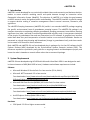
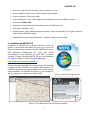
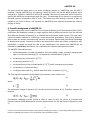
uWATER–PA:
Ubiquitous WebGIS Analysis Toolkit for Extensive Resources
Pumping Assessment
Version 1.0
User’s Manual
Yi-Chen E. Yang
Yu-Feng F. Lin
Miscellaneous Publication 194
Illinois State Water Survey
Prairie Research Institute
University of Illinois at Urbana-Champaign
June 30, 2011
Revision: October 27, 2011
Illinois Non-Exclusive Research Use License
http://www.isws.illinois.edu/gws/sware/agreement.asp?pkg=uwsw&sp=pg1
uWATER–PA
1. Introduction
uWATER is a tool developed for non–technically minded citizens and community and business decisionmakers to access scientific modeling results and spatial datasets through an interactive online
Geographic Information System (WebGIS). The objective of uWATER is to bridge the gap between
scientific research results and general public understanding. The uWATER interface is general enough
to support decision making in numerous management issues in natural resources, economics, and
agriculture.
The uWATER–Pumping Assessment (uWATER–PA) toolkit is an extended uWATER package targeting
the specific environmental issue of groundwater pumping impacts. The uWATER–PA package is an
excellent alternative to evaluating complex groundwater pumping assessment issues before investing
significant time, labor, and funds in monitoring and detailed scientific study. It incorporates simulation
of the physics of groundwater flow and user interaction into GIS software. A graphical user interface
makes both data entry and interpretation of results intuitive to non-technical individuals. Results are
presented as colored maps showing well drawdown (change in groundwater level), and these results
can be saved in GIS format for future reference.
Both uWATER and uWATER–PA are free-download plug-in packages for the free GIS software ArcGIS
Explorer Desktop (AGX) developed by the Environmental Systems Research Institute (ESRI). This
document represents a preliminary user guide for an ongoing research and development project, and
hence the code is viewed as a research effort rather than a commercial package.
2. System Requirements
uWATER–PA was developed using AGX SDK with Microsoft Visual Basic 2008. It was designed to work
in the environment of AGX (Build 1500 or later). Hardware and software requirements include:
Software

Microsoft Windows XP Service Pack 2 or later version (32 bit, 64 bit)

Microsoft .NET Framework 3.5 or later version
Free download at: http://www.microsoft.com/downloads/details.aspx?FamilyId=5b2c0358915b-4eb5-9b1d-10e506da9d0f&displaylang=en

Microsoft XML Core Services (MSXML) 4.0 Service Pack 2 or later version
Free download at: http://msdn.microsoft.com/en-us/data/bb190600.aspx

Internet Explorer 7.0 or later version
Free download at: http://www.microsoft.com/windows/internet-explorer/default.aspx

ArcGIS Explorer Desktop (Build 1500 or later)
Free download at: http://www.esri.com/software/arcgis/explorer/download.html
Hardware

CPU Speed: 2.2 GHz or higher recommended
1
uWATER–PA

Processor: Intel Core Duo, Pentium 4, Xeon Processors or later

Memory/RAM: 1 GB minimum, 2 GB or higher recommended

Display Properties: 24 bit color depth

Screen Resolution: 1024 x 768 or higher recommended at normal size (96dpi); the best
resolution is 1680 x 1050

Swap Space: Determined by the operating system, 500 MB minimum

Disk Space: 300 MB or more

Video/Graphics: 24-bit capable graphics accelerator, video card OpenGL 2.0 or higher compliant,
video memory 256 MB or higher

Bandwidth Connection Speed (optional): 1.5 Mbps or higher recommended
3. Installation of uWATER–PA
Installation of uWATER–PA is simplified because it does not
require a conventional executable file (such as an .exe or .dll
file) on the destination computer. Instead, uWATER–PA uses an
AGX Application Configuration file (.ncfg) that installs
automatically on any computer on which AGX is properly
installed. To begin installing uWATER–PA, one must download
the .ncfg file (Figure 1) from the program Web page:
http://www.isws.illinois.edu/gws/sware/
Double-clicking the uWATER–PA.ncfg icon opens AGX and adds
a customized tab, uWATER, to the default AGX interface. The
uWATER tab includes two control buttons that, when clicked,
launch uWATER1.1 or uWATER–PA (Figure 2), the interface of Figure 1. The uWATER–PA ArcGIS
which is designed as a dockable window in AGX.
Explorer Application Configuration file
Figure 2. The uWATER tab in ArcGIS Explorer Desktop
2
uWATER–PA
The users should be aware there is no actual installation process for uWATER-PA after the AGX is
installed. Starting uWATER-PA is like opening a word file (.doc), and the MS-WORD program starts
along with it. Therefore, uWATER-PA will not be available if the user only starts AGX, which is similar to
opening MS-WORD but not opening a word file (.doc). The advantage of this process is to significantly
decrease technical maintenance from IT staff. The default map area setting is zoomed to (but not
limited to) the State of Illinois, USA, because the uWATER-PA was originally developed for research
projects in Illinois.
4. Scientific background of uWATER–PA
The governing equation used in uWATER–PA to compute drawdown is the Theis equation (Theis, 1935).
It describes the drawdown caused by a single pumping well at different distances from the well and
after different durations of pumping in an idealized two-dimensional aquifer system. There are many
numerical models available for simulating a three-dimensional groundwater flow system. However,
these models are usually computationally intensive and require sophisticated professional knowledge
to develop and operate. Assuming a uniform two-dimensional system will reduce computation time
significantly. It should be noted that due to this simplification, the results from uWATER–PA are
intended as a preliminary assessment, not a replacement of sophisticated numerical models.
The uWATER–PA model assumes:

an idealized pattern of radial groundwater flow surrounding a single, constantly pumping well
open to an infinitely-extending (i.e., no boundaries) confined aquifer* (Figure 3)

the pumping rate of this well is Q [L3/T]

the pumping duration is t [T]

the transmissivity of the confined aquifer is T [L2/T] and it is assumed to be isotropic

the storativity is S [dimensionless]

the original water level is h0, and the water level after t at distance r [L] is h(r,t).
The Theis equation expresses the drawdown (s) at distance r after duration t as:
(1)
where
(2)
The exponential integral in Equation (1) is known as the well function: W (u). Therefore, equation (1)
becomes:
(3)
Groundwater textbooks typically provide a table of values of W(u) for various u. Srivastava and
Guzman-Guzman (1998) developed an accurate approximation for the well function (Equations 4 and
5):
3
*Users have to be careful that if the aquifer is NOT infinitely-extending, boundary (i.e., aquifer edge) effects might occur and
results from uWATER-PA will require more interpretation from groundwater experts.
uWATER–PA
(4)
(5)
where C1 is Euler’s constant, i.e. C1 = 0.5615
Figure 3. Drawdown surrounding a single pumping well open to a confined aquifer (modified from
Freeze and Cherry, 1979)
For the uWATER–PA drawdown computation, the pumping rate (Q) and the pumping duration (t) of the
new well are required as user inputs. The transmissivity (T) and storativity (S) of the confined aquifer,
which are critical controls of groundwater flow in the aquifer, are also required inputs. The existing
wells locations are required for the well impact assessment. Presently, a grid-based shapefile is the
only format currently acceptable in uWATER–PA for T and S inputs. Since the distance calculation is an
inherent capability of AGX, the distance (r) is easily computed and used in the above functions. Using
all of these parameters, uWATER–PA will compute the drawdown(s) in the vicinal cells of the new well.
Transmissivities are computed using the geometric mean of arithmetic and harmonic mean along the
shortest path between the vicinal cells and the new well as suggested by De Lucia et al., 2009.
Therefore, the transmissivity in each cell will be different and, to a certain degree, approximates a
heterogeneous aquifer.
5. uWATER–PA Interface
The uWATER–PA interface includes three major tabs (Figure 4). The Data Input tab (Figure 4a) is used
to define units and to import the necessary data from AGX to uWATER–PA. The Impact Assessment tab
(Figure 4b) is employed to specify the properties of the proposed new pumping well and the display
settings for the computation and results. The Impact System (Figure 4c) tab shows the legend used to
display the significance of the additional drawdown caused by the new pumping well. This legend is
4
uWATER–PA
based on the ratio between the additional drawdown at one location to the maximum additional
drawdown at the proposed new pumping well location.
(a)
(b)
(c)
Figure 4. The uWATER–PA interface: (a) Data Input, (b) Impact Assessment, (c) Impact System
The user must first select the units to be used in uWATER–PA (Figure 4a). For common management
usage, these units may be U.S. customary units (miles for distance, ft2/day for transmissivity, and
gallons/day for pumping rate) or S.I. Metric (kilometers for distance, m2/day for transmissivity, and
liters/day for pumping rate). The button Add a well on the map using the cursor then allows the user to
directly locate the new well anywhere on the map. This second step employs direct user-software
interaction, making the decision process visual and intuitive. The user also must enter a Distance of
Interest (i.e., a radial distance from the well within which results will be displayed). Alternatively,
marking a check box will cause results to be displayed for the entire aquifer. The third step is to import
transmissivity (T) and storativity (S) data from AGX into uWATER–PA. Shapefiles containing these data
must be preloaded into AGX; the user selects each shapefile with the cursor, displays its attributes, and
selects the attributes representing transmissivity and storativity. A similar procedure is required to
import a shapefile representing existing wells from AGX into uWATER–PA.
The Impact Assessment tab (Figure 4b) allows the user to enter maximal and actual pumping rates and
durations. Sliding bars provide a convenient way to use different pumping rates and durations.
Optionally, the user can check a box to show the drawdown distribution as a color-coded impact map.
Otherwise uWATER–PA will only show the impacted wells (automatically generated results using
spatial query in uWATER-PA) using a color-coded system. When the pumping rates and durations have
been entered, the user clicks either the Compute Impact with Maximal Pumping button or the
Compute Impact with Actual Pumping button for additional drawdown calculation.
5
uWATER–PA
It should be noted that uWATER–PA does not require a predevelopment water-level surface as input
data, so the program output consists of additional drawdown caused by the proposed new pumping
well. The absolute value of additional drawdown is given in the pop-up window of each cell. The
maximum additional drawdown value caused by pumping from the proposed well is used for
normalization of the result display. The impact in areas within the designated radius surrounding the
proposed well is shown using color coding adapted from the Homeland Security Advisory System
(Figure 4c). The degree of impact is calculated using the impact ratio (Figure 5), which is the ratio of the
additional drawdown in a cell to the maximum additional drawdown (i.e., the drawdown in the cell
containing the proposed well). Areas with extreme, high, elevated, perceptible, and low impacts are
shown in red, orange, yellow, blue, and green, respectively. The same color scheme is used for the
impacts on existing wells. Note that, regardless of the input data and grid size, the grid cell containing
the proposed pumping well is always red because the impact ratio within the cell is always 1.
Extreme
high
elevated
perceptible
low
Figure 5. The calculation of impact ratio in uWATER–PA (not with real scale)
6. Example
An example using McHenry County, Illinois as a hypothetical case is provided in this section to
demonstrate the functionality of uWATER–PA. This example illustrates the computation of additional
groundwater drawdown caused by a potential well and its impacts on existing wells. It should be noted
that uWATER-PA itself is only a toolkit and does not contain any dataset (e.g. T, S, and existing wells
location). All files downloaded with uWATER-PA are only used for demonstration purposes. Since
transmissivity (T) and storativity (S) data are neither nationally nor globally available, more
hydrogeological studies to enlarge this database will certainly increase the benefit of uWATER-PA and
are strongly suggested by the development team. Meanwhile, the results of uWATER-PA can be saved
(right-click on the resulted layer) as Map Content Files (.nmc), (the default of AGX). It should be noted
that AGX and its plug-in cannot create a shapefile, which is intentionally restricted by the ESRI.
Therefore, model parameters such as pumping rates and durations cannot be saved.
6
uWATER–PA
1) Launch the uWATER–PA main program. Under the “Home” tab, use the Add Content button to
browse and add the shapefile McHenry_T.shp, McHenry_S.shp and McHenry_wells_L14.shp in the
uWATER–PA-testdata folder downloaded with the program (Figure 6). McHenry_wells_L14.shp
contains the locations of existing wells pumping from flow model layer 14, the Ancell Unit, which
will become the impact assessment target in this example.
Figure 6. Adding the required shapefiles.
2) Under the “uWATER” tab, click the uWATER–PA button to open the uWATER–PA interface. The
interface is designed to be docked along with “Contents.” Select the “U.S. Customary Units”
radiobutton since the unit of transmissivity used here is ft2 per day (Figure 7).
Figure 7. Selecting U.S. Customary Units.
7
uWATER–PA
3) Click Add a well on the map using the cursor button on the uWATER–PA interface and move the
cursor to the map. The cursor will become a cross, and the user can click on the map to locate the
potential well. In this example, a site in the middle of McHenry County is chosen. The potential well
is displayed as a glass of water. After locating the potential well, type in “8” miles as the “Distance
of Interest” on the uWATER–PA interface (Figure 8).
Figure 8. Using the cursor to add a potential well directly to the map.
4) Use the cursor to highlight mchenry_t.shp in “Contents” and click the Select Transmissivity layer
button on the uWATER–PA interface. The selected transmissivity layer will display on the uWATER–
PA interface (Figure 9).
Figure 9. Selecting the transmissivity layer shapefile.
8
uWATER–PA
5) Click on the Show attributes button on the “Data Input” tab. All attributes in the selected
transmissivity layer will display in the dropdown list. In this example, there are 21 columns
representing the transmissivity data for 21 geological layers. Highlight T14 from the dropdown list
since wells pumped from geological layer 14 are the targets in this example (Figure 10).
Figure 10. Identifying the transmissivity of geological layer 14: “T14.”
6) Follow a similar procedure as in steps 4 and 5 to identify the characteristics of storativity with
mchenry_s.shp and highlight S14 from the dropdown list (Figure 11).
Figure 11. Identifying storativity characteristics.
9
uWATER–PA
7) Use the cursor to highlight mchenry_wells_l14.shp in “Contents” and click the Select wells layer
button on the “Data Input” tab. The selected well layer will display on the uWATER–PA interface
(Figure 12). This step completes the Data Input procedure.
Figure 12. Selecting the existing wells shapefile.
8) Click the “Impact Assessment” tab on uWATER–PA interface and check the “Show the drawdown
distribution (more time needed)” checkbox. This procedure will allow additional drawdown
distribution to be shown in the final results (Figure 13).
Figure 13. Checking “Show the drawdown distribution (more time needed)”.
10
uWATER–PA
9) Type in 200,000 gallons per day as the maximal pumping rate and use the slide bar to select
100,000 gallons per day as the actual pumping rate (Figure 14). This design allows users to change
actual pumping rate in the future if necessary.
Figure 14. Inputting the pumping rate information.
10) Repeat step 9 for the pumping duration. Use 365 days as the maximal duration and 30 days as the
actual duration (Figure 15).
Figure 15. Inputting pumping duration information.
11
uWATER–PA
11) Click the Compute Impact with Maximal Pumping button to compute the results. The progress bar
will show the current progress (Figure 16). Since the Compute Impact with Maximal Pumping
button is clicked, uWATER–PA will ignore the current pumping rate and duration. The resulting
drawdown will be calculated using maximal pumping rate and duration.
Figure 16. Computing the results.
12) Because “Show the drawdown distribution (more time needed)” has been checked, when the
program finishes, a folder “Impact ratio (Maximum Impact)” will be created with additional
drawdown distribution. The user can click the “Impact System” tab on the interface to show the
additional drawdown legend. The color scheme illustrates the degree of impact for each cell. The
user can also click on any cell and a pop-up window will display. The pop-up window provides
detailed information about the additional drawdown caused by the potential well (Figure 17).
Figure 17. Displaying the results of the additional drawdown distribution.
12
uWATER–PA
13) A folder titled “Interested mchenry_wells_l14 within 8 miles (Maximum Impact)” will be created
with all impacted existing wells. The default symbol for impacted wells is a pushpin. The same color
scheme as for the impact ratio is used with the pushpins to illustrate the degree of impact on each
well. Pop-up windows will also display when the user clicks on wells he or she is interested in.
Detailed information about additional drawdown near this well will be displayed (Figure 18).
Figure 18. Displaying the impact on existing wells.
7. Future Development
At the bottom of the uWATER–PA interface “Data Input” tab, the developer reserved a place to
preview future developments in stream depletion analysis for which uWATER-PA will be used to
estimate the stream depletion impact caused by a new pumping well. This function is currently
disabled but is scheduled to be released in the next version. Another ongoing development is to add
the computation function for Map Content Files (.nmc) which allows users to compare the difference
between two uWATER-PA simulations.
8. Known Issues Related to Operation
One known issue in the current version is the adjustment of display resolution. The suggested
resolution is 1680 x 1050, which is the best resolution to display the uWATER-PA interface. A higher
resolution will have no problem operating the interface, but some blank areas might appear on the
screen. A lower resolution (e. g. 1024 x 760) will encounter some difficulties in fully displaying the
interface. In this case, the user has to undock the interface from the AGX main program and adjust the
boundary to display all buttons on the interface. This issue has no effect on the computation results
although the display of the interface might seem unbalanced.
There might be two versions of AGX (Build 1700) available for download; one requires administrative
permissions to install and the other does not. The former version with administrative permissions is
fully compatible with uWATER-PA if ArcGIS 10.0 is installed on the test system.
13
uWATER–PA
9. Acknowledgements, Availability, and References
Support for development of uWATER and uWATER–PA was provided by McHenry County, Illinois, USA
and the State of Illinois. This revision was updated mainly based the test by J. Fernando Rios
(University at Buffalo), Ming Ye (Florida State University), and Liying Wang (Florida State University).
Their technical review (Rios et al., 2011) was very helpful and highly appreciated. The uWATER and
uWATER–PA packages (program, example files, and user’s manual) are free to download at
http://www.isws.illinois.edu/gws/sware.
Please contact Yu-Feng Forrest Lin ([email protected]) for questions or comments.
The citations for the software and manual are as follows:
Yang, Y. C. E. and Lin, Y. F. (2011) uWATER-PA: Ubiquitous WebGIS Analysis Toolkit for Extensive
Resources – Pumping Assessment, User’s Manual. Illinois State Water Survey, Prairie Research Institute,
University of Illinois at Urbana-Champaign.
Related articles are available at:
Yang, Y. C. E. and Lin, Y. F. (2011) A New GIScience Application for Visualized Natural Resources
Management and Decision Support. Transactions in GIS 15 (s1): 109-124.
Yang, Y.C. E. and Lin, Y.F. (2011) Feature Article: Making the Results of Analysis Accessible: ArcGIS
Explorer plug-in aids natural resources management. ArcUser 14, no. 1: 22 - 25.
http://www.esri.com/news/arcuser/0111/uwater.html
Freeze, R. A. and Cherry, J. A. (1979) Groundwater. Prentice-Hall, Inc. Englewood Cliffs, NJ. 604 pp.
De Lucia, M., de Fouquet, C., Lagneau, V. and Bruno, R. (2009) Equivalent block transmissivity in an
irregular 2D polygonal grid for one-phase flow: A sensitivity analysis. C. R. Geoscience, 341: 327–
338.
Rios, J.F., Ye, M., and Wang, L. (2011) Software Spotlight - uWATER-PA: Ubiquitous WebGIS Analysis
Toolkit for Extensive Resources – Pumping Assessment. Ground Water 49, no.6: 776-780. DOI:
10.1111/j.1745-6584.2011.00872.x
14