1
User's Manual
Composite Compressive
Strength Modeller
A Windows™ based composite design tool
for engineers
Version 2.0
2013
M. P. F. Sutcliffe†, X. J. Xin†,
N. A. Fleck† and P. T. Curtis*
†
Engineering Department
Cambridge University
Cambridge, CB2 1PZ, U.K.
*
DSTL Farnborough
GU14 0LW, U.K.
CONTENTS
1. INTRODUCTION .............................................................................................................................4
2. INSTALLATION ..............................................................................................................................5
2.1 System requirements............................................................................................................5
2.2 The CCSM package.............................................................................................................5
2.5 Setting up CCSM.................................................................................................................5
3. QUICK START ...............................................................................................................................5
3.1 How to use CCSM...............................................................................................................6
3.2 A quick start example ..........................................................................................................7
4. DETAILED GUIDE AND ADVANCED TUTORIALS ............................................................................13
4.1 Nomenclature convention in CCSM..................................................................................13
4.2 Details for each form .........................................................................................................17
4.2.1 Laminate elastic properties forms .............................................................................17
4.2.2 Elastic Properties Tutorial.........................................................................................19
4.2.3 Deformation analysis ................................................................................................21
4.2.4 Deformation Analysis Tutorial .................................................................................21
4.2.5 Failure analysis .........................................................................................................23
4.2.5.1 Conventional Failure Criteria ................................................................................23
4.2.5.2 BFS Failure Criteria...............................................................................................24
4.2.6 Conventional Failure Analysis Tutorial....................................................................25
4.2.7 BFS Compressive Failure Analysis Tutorial ............................................................27
4.3 Materials Databases...........................................................................................................29
4.3.1 DataBase (Elastic Property Data) .............................................................................29
4.3.2 DataBase (Strength):.................................................................................................29
4.3.3 Database for the bridging analysis............................................................................29
APPENDIX A THEORETICAL BACKGROUND ....................................................................................31
A.1 Lamina stress-strain relationships.....................................................................................31
A.1.1 The orthotropic lamina.............................................................................................31
A.1.2 The generally orthotropic lamina.............................................................................34
A.2 Classic laminate theory (with bending) ............................................................................36
A.3 Laminate compliances ......................................................................................................40
A.4 Determination of lamina stresses and strains....................................................................40
A.5 Conventional lamina failure criteria .................................................................................41
A.5.1 Maximum stress .......................................................................................................41
A.5.2 Maximum strain .......................................................................................................41
A.5.3 Tsai-Hill ...................................................................................................................42
A.5.4 Tsai-Wu....................................................................................................................42
A.6 BFS compressive failure criterion ....................................................................................43
A.7 Laminate failure analysis..................................................................................................45
A.8 Failure of notched laminates.............................................................................................45
A.9 Interpolation and extrapolation of the bridging analysis data ..........................................50
A.9.1 For points inside the macro grid of the look-up table ..............................................51
A.9.2 For points outside the macro grid of the look-up table ............................................53
B.10 References.......................................................................................................................55
2
Acknowledgements
The authors are grateful for helpful advice from Dr C Soutis, Ms V Hawyes, Mr P Schwarzel and
Mr I Turner, for additional programming help from Mr A Curtis and for financial support from
the Procurement Executive of the Ministry of Defence, contract 2029/267, and from the US
Office of Naval Research grant 0014-91-J-1916.
Disclaimer: Although the calculations and implementation in this program are believed to be
reliable, the authors cannot guarantee the accuracy of the results produced by this program and
shall not be responsible for errors, omissions or damages arising out of use of this program.
3
Composite Compressive Strength Modeller
User's Manual
1. Introduction
Welcome to the Composite Compressive Strength Modeller (CCSM) – a design tool for
deformation analysis and failure prediction of composite materials.
CCSM incorporates the following features:
1. Classical laminate theory for the prediction of laminate elastic properties;
2. Stress and strain analysis when in-plane forces and/or bending moments are applied;
3. Unnotched failure prediction by conventional failure criteria and the Budiansky-Fleck
compressive failure criterion;
4. Compressive failure prediction for notched composite plates.
5. A user-expandable database to store material and geometrical properties.
The program is a tool to predict laminate failure, once the loads on a section of the laminate are
known. For simple geometries it may be clear what the loading is, while for more complicated
geometries the program may be used as part of a larger calculation to check for failure at critical
points in the structure.
CCSM is written in Microsoft® Visual Basic TM language using Visual Studio 2012and it runs in
TM
operating system. It is structured so that the user, with a basic
the Microsoft® Windows
knowledge of composite mechanics, can use it with little reference to the manual. However, the
user would benefit from reading through this manual, in particular the Quickstart section, chapter
3 and the detailed guide, chapter 4. CCSM 2.0 updates and simplifies Version 1.4.
This manual consists of the following chapters:
1. Introduction.
2. Installation:
Instructions on how to install CCSM
3. Quick Start:
A 'quick start', self-sufficient chapter illustrating how to
use the CCSM package.
4. Detailed guide
Detailed guide to all aspects of the program with tutorials
Appendix A
Theoretical Background: underlying principles of CCSM
4
2. Installation
2.1 System requirements
CCSM uses Microsoft .NET Framework 4 (or above) which needs to be installed before running
the application.
2.2 The CCSM package
The CCSM deployment file contains the following items:
* User's manual;
* A Quickstart manual;
* Application and data files.
2.5 Setting up CCSM
To install CCSM run the setup.exe program. If you want to change the database then you will
need write permission for CCSM.MDB.
3. Quick Start
This chapter contains an introductory example of the use of CCSM. The chapter is intended to be
followed at a computer running CCSM: commands and data to type in to CCSM are listed.
CCSM is written in Visual Basic (VB), a package designed to produce especially user-friendly
graphical interfaces. The user should work through the various forms in CCSM by following the
logic of a problem. For example, in order to calculate the stiffness of the laminate, sufficient
information about each lamina should be provided first. Similarly, analysis of stress and strain
would be meaningless without previously calculating the laminate properties and specifying the
applied loads.
CCSM contains a number of forms for each stage of the analysis. Details at each stage are filled
in using text boxes containing data, option buttons, and command buttons.
5
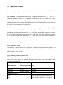
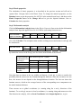
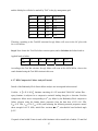
3.1 How to use CCSM
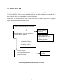
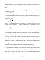
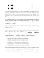
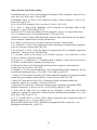
The following flow chart shows what to do in CCSM. In each form in CCSM corresponding to
each box in the flow chart, there is an information box providing information about what to do
next. Boxes in which to input data have a white background.
Further help can be obtained from the ? buttons and from the manual. Details of the program
authors are included using the About button.
Start CCSM by clicking the CCSM icon
from within Windows
Use the database
if needed
Elastic properties: input ply properties;
calculate laminate stiffness
either
or
Use the More Elastic
Properties form to look at
further laminate and ply
stiffness properties
Deformation analysis:
Calculate stresses and
strains for each ply
Failure analysis:
Calculate unnotched and
notched strength
Use the database
if needed
A flow diagram showing the structure of CCSM
6
3.2 A quick start example
This section goes through a simple analysis to illustrate the essential features of CCSM. More
advanced tutorials are given in chapter 4.
The problem.
Determine the stiffness and compliance matrices for a [0 o / ± 45o / 0o ]s
symmetric laminate consisting of 0.1 mm thick unidirectional AS/3501 carbon fibre – epoxy
laminae. Also find the stresses and strains for each lamina when the laminate is subjected to a
single uniaxial force per unit length Nx=200 MN/mm. Use the Tsai-Wu failure criterion to decide
the load level corresponding to first ply failure.
The following lamina stiffness and strength data are given: longitudinal modulus E11=138 GPa,
transverse modulus E22=9 GPa, shear modulus G12=6.9 GPa, Poisson's ratio ν12=0.3,
longitudinal tensile strength, denoted as SL(+)=1448 MPa, longitudinal compressive strength,
SL(-)=1172 MPa, Transverse tensile strength, ST(+)=48.3 GPa, Transverse compressive strength,
ST(-)=248 GPa, in-plane shear strength, SLT=62.1 GPa (taken from R. F. Gibson's Principles of
Composite Material Mechanics, Table 2.2, P.48, 1994).
A step by step illustration is given below:
Step 1: Starting CCSM
After starting Windows, launch the Compressive Composite Strength Modeller program. The
Geometry and elastic analysis: form is then loaded automatically and the cursor will be blinking
in the Composite name text box.
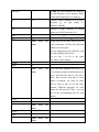
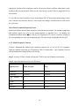
Step 2: Entering elastic properties data.
In this step laminate data and elastic properties are entered. All white text boxes are input boxes,
and the light yellow boxes are output or information boxes. Now type in the following data,
according to the problem:
Which input box
What you type or do Note
Composite:
AS/3501
Optional
Comments:
Quickstart example
Optional
Total number of plies
8
Ply No.
1
Type the current ply number into this box
Angle
0
Type the angle into this box (in degrees)
7
Thickness
In mm The total thickness box displays
0.1
the total thickness of the laminate, based
on the entered thicknesses for each ply.
E11
138
Lamina's Young's modulus in first (fibre)
direction E11 (in local lamina coordinates), in GPa
E22
9
Lamina's Young's modulus in second
(transverse to fibre) direction E 22
Nu12
0.3
Poisson's ratio ν12
G12
6.9
In-plane shear modulus G12
(click
Data)
Ply No.
2
Angle
45
(click
Data)
Ply No.
3
Angle
-45
(click
Data)
Ply No.
4
Angle
0
(click
Data)
Save
Ply At this point, all necessary data for ply No.
1 have been input. Click the Save Ply Data
button to save the input.
The ply arrangement grid is filled for each
ply where data has been saved.
For ply Nos. 2 to No 4, the input
procedures will be similar.
Save
Ply Notice that after inputting data for ply No.
1, the Lamina properties and thickness text
boxes still hold the data for Ply No.1.
Those data, because expressed in local
lamina co-ordinate, are valid for other
plies as long as they are for the same
material. Different properties for each
lamina are allowed in CCSM – you just
type in the corresponding data for each
lamina.
Save
Ply
Save
Ply
8
Ply Nos. 5-8
Ply data for plies 5-8 have been
automatically filled in, because the
laminate type option is by default
symmetric. The ply geometry and
property data are symmetrical about the
centre line.
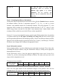
Step 3. Calculating the stiffness of the laminate
At this point, data for all laminae have been entered. Now click the Calculate button to calculate
the laminate stiffness. The first 5 components represent E x , E y , Gxy , ν xy and ν yx , for the
laminate, using standard notation for an orthotropic laminate. The sixth component, E' , is the
appropriate elastic modulus for an orthotropic material such that G = K2 / E' , where G is the
elastic energy release rate and K is the mode I stress intensity factor. Further details of the
meanings of these symbols are given in the Theory section, Appendix B.
Section 4.2.1 covers in more detail the various controls on the Elastic analysis form. In particular
it explains in detail how the Ply Input, Ply Editing and Change All tools can be used to speed
up the input and modifications to the laminate geometry. In brief, the different columns in the Ply
Input tool refer to different angles required for the Previous, Current (=) and Next ply. Click Save
Ply Data to store changes after clicking on the appropriate button.
Step 4 Deformation analysis
In our example problem, we wish to find the stresses and strains in each ply. This is done, after
calculating the laminate stiffness, using the Deformation Analysis, clicking on the appropriate
button under the GoTo tool.
On the Deformation analysis: form, first input the applied load, in this case 0.2 in the Force
resultant Nx text box (converting from MN/mm to MN/m). The other text boxes can be left
empty as these components are zero.
The input text boxes should be:
Force resultants
Nx
on laminate
0.2
Ny
N xy
Mx
My
M xy
This is the only input needed for the deformation analysis in this problem. Now click the
Calculate button. The mid-plane strains and curvatures will be calculated, and shown as:
Mid-plane strains
Ex
Ey
Gamma xy
Kx
Ky
K xy
and curvatures
3075
1934
~0.
~0.
~0.
~0.
9
where ~0 is a very small value (of the order of rounding errors). The mid-plane shear strain γ xy
(Gamma xy) and all curvatures are zero, because the laminate is symmetric and there are no
bending components.
Though the stresses for all plies have been calculated, only stresses in one ply will be shown in
the Stress State grid (the first ply by default). Stresses at the top, middle and bottom of each
selected ply are shown; this takes into account the possibility of linear variation in the stress in
the presence of bending. At the present example, the stresses in each ply is constant. The bottom
row shows the average stress through the full thickness of the laminate. The results are shown as:
Through
thickness t
Stress state for ply No. 1
of selected
ply
Sigma_x
Sigma_y
Tau_xy
top
421.697
-9.161
0.
middle
421.697
-9.161
0.
bottom
421.697
-9.161
0.
Laminate
stresses
250
0.
0.
These stresses are in global coordinates (i.e. running along the x and y directions of the laminate).
To see the ply stresses in local coordinates (i.e. running along and transverse to the fibre direction
in each ply), click on the appropriate Output Option.
To display the ply stresses of other plies, navigate through the ply arrangement grid either
clicking with a mouse or using cursor keys. The current ply is highlighted in this grid.
Notice that in the Output Option box, the "stress" option is set as the default. Clicking the
"strain" option will display strain data giving:
Through
thickness t
Strain state for ply No. 1
of selected
ply
Epsilon_x
Epsilon_y
Gamma_xy
top
3075
-1934
~0.
middle
3075
-1934
~0.
bottom
3075
-1934
~0.
Laminate
strains
10
Note that strains are output in microstrain. It can be seen that there are stress discontinuities at the
ply interfaces, while the strains are continuous across the interface:- this reflects the basic
assumption of the classical laminate theory.
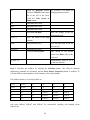
Step 5: Failure analysis
To predict laminate failure, click on the Failure Analysis button, once the laminate properties
have been entered and the laminate stiffness calculated.
There are five failure analysis criteria available in CCSM: the maximum stress, the maximum
strain, the Tsai-Hill, the Tsai-Wu and the Budiansky-Fleck-Soutis (BFS) compressive failure
criteria. All these criteria are lamina failure criteria. Select the "Tsai-Wu" option for the present
problem.
Now type in the following strength data for the material AS/3501:
Which input box:
What you type:
Note
Longitudinal tensile strength SL(+)
1448
In MPa.
Longitudinal compressive strength SL(-)
1172
Transverse tensile strength ST(+)
48.3
Transverse compressive strength ST(-)
248
In-plane shear strength SLT
62.1
Click on the Save Data - All Plies button, to store this data.
Instead of typing the above data in each input text box, you can make use of the Database menu.
Click on the Database button. All relevant data which have been stored in the database will
appear in the list box on the left side of the form. Click on the required material's name in this
list, which is 'AS/3501' in the present example, then click the Take record as input button. You
will return to the Failure analysis form with the selected strength data displayed in the
appropriate input text boxes. Now click on the Save Data - All Plies button as before.
Finally we need to input the Force pattern which is applied to the laminate. Enter the appropriate
data in the force input boxes, e.g.
Force pattern
Nx
applied to laminate
0.2
Ny
N xy
11
Mx
My
M xy
Note that it is only the ratio of forces that is required here, so that a pattern
Force pattern
Nx
applied to laminate
1
Ny
N xy
Mx
My
M xy
would convey exactly the same information.
When the necessary data for the failure analysis have been input, click the Calculate button. The
output boxes below the input force pattern show the failure loads,
Forces to give failure
Nx
Ny
N xy
Mx
My
M xy
0.327
0
0
0
0
0
telling us that the force to cause the first ply failure, when the Tsai-Wu failure criterion is
applicable, will be Nx=0.327 MN/m with Ny=Nxy=Mx=My=Mxy=0. The magnitude of the
input load Nx=0.2 MN/m will not affect the actual value of the failure load Nx. The relative
magnitudes of the load components are determined by the input values of Nx: Ny: Nxy: Mx: My:
Mxy ; the failure loads scales with this load pattern.
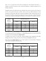
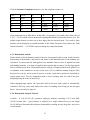
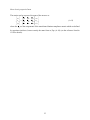
Observe also that in the ply arrangement grid on the left side, the fourth column marked "Fails
first?" shows which plies have failed. For the present case, all the 45/-45 degree plies fail at the
same time. Hence the grid appears as:
No.
Angle
Thick.
Fails
first?
1
0
0.1
2
45
0.1
Yes
3
-45
0.1
Yes
4
0
0.1
5
0
0.1
6
45
0.1
Yes
7
-45
0.1
Yes
8
0
0.1
In this section we have covered the Tsai-Wu failure criterion for unnotched strength. The
advanced tutorials in Section 4.2 give further information on the failure analysis, including an
illustration using the Budiansky-Fleck-Soutis model for compressive failure, and the prediction
of both the unnotched and the notched strength of laminates.
12
4. Detailed guide and advanced tutorials
This section is a detailed guide to the use of CCSM. Section 4.1 contains information about the
nomenclature used in CCSM. Section 4.2 contains further information and advanced tutorials for
each form in CCSM. To help use the full capability of CCSM, it is suggested that you go through
these tutorials. Finally section 4.3 contains details of the databases used by CCSM.
4.1 Nomenclature convention in CCSM
This section describes in detail the nomenclature used in CCSM.
Global co-ordinate: the two co-ordinates of the global (laminate) system are denoted by x and y.
The first axis of the global co-ordinate system, the x axis, coincides with the fibre direction of the
0 degree plies.
Local co-ordinate: the two axial directions of the local co-ordinates of a lamina are denoted by 1
and 2. The first axis of the local (lamina) co-ordinate system, the 1 axis, coincides with the fibre
direction of the lamina.
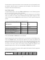
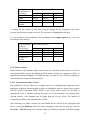
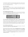
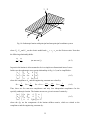
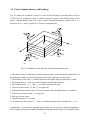
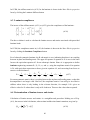
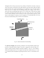
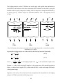
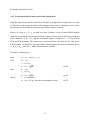
The sign convention for lamina orientation with relation to the global co-ordinate is illustrated in
Fig. 1.
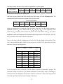
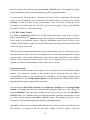
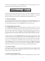
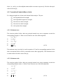
The stress resultants used for the laminate analysis are defined in Fig. 2.
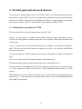
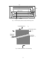
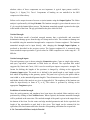
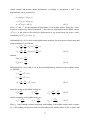
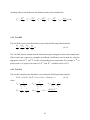
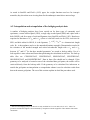
The laminated plate geometry and ply numbering system is illustrated in Fig. 3.
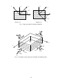
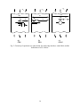
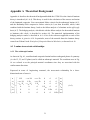
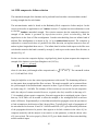
The nomenclature for the Budiansky-Fleck-Soutis compressive failure theory is illustrated in Fig.
4. For the compressive failure case, the stress in the longitudinal fibre direction σL will be
negative.
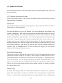
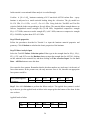
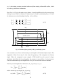
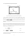
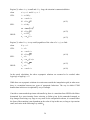
The definitions of a or R, b, and w for the three types of specimens for the bridging analysis are
shown in Fig. 5. Note that for the centre notch panels a and w are the semi-notch length and the
semi-width of the specimen.
13
2
Y
1
Y
2
+θ
X
X
−θ
Negative θ
Positive θ
1
Fig. 1 Sign convention for lamina orientation.
Z
X
Y
Mx
My
Nxy
Nx
Mxy
Nyx
Myx
Ny
Fig. 2 Coordinate system and stress resultants for laminates plate.
14
top
1
2
t
Z(0)
Z(2) Z(1)
middle surface
Z(k-1)
k
t/2
Z(k)
Z(N)
N
Z
bottom
Fig. 3 Laminate plate geometry and ply numbering system.
Longitudinal stress
τ
−σ
L
Transverse stress
σ
T
Kink band
inclination
Initial fibre
waviness φ
β
Fig. 4 Infinite band model of microbuckling
15
2w
(a)
CEN
2w
w
b
l
L
L
L
2a
−σ
−σ
−σ
a
b
2R
l
(b)
SEN
b
l
(c)
HOLE
Fig. 5 Geometry of specimens (a) centre notch, (b) single edge notch (c) central hole, and the
definitions of a, R, b and w.
16
4.2 Details for each form
More detailed information on each of the separate forms are grouped together in this section, with
associated tutorials.
4.2.1 Laminate elastic properties forms
In this section further features of the Geometry and Elastic Analysis and More Elastic Laminate
Properties forms are explained.
Introduction
The laminate geometry and lamina elastic properties are input in this form. Boxes in which to
input data have a white background.
First enter the number of plies in the laminate. Click on the appropriate option button if the
laminate is unsymmetric. Then enter the elastic properties, thickness and ply angle of the first ply
and click Save Ply Data. It is assumed by default that all plies have the same properties and ply
thickness, although this can subsequently be overwritten by typing in data for each ply and saving
the ply data. A composite name and comments are optional and can be entered at any time. The
database button accesses a database of lamina elastic properties. Use the ply arrangement box to
navigate through the plies, either by clicking on the relevant ply or using cursor keys, to see the
saved material properties. When all the ply data have been saved, the laminate properties are
calculated using the Calculate button. The total thickness box displays the total laminate
thickness, based on the ply thicknesses entered.
Materials Data Input Option
There are two choices for defining the elastic data for each ply. The Engineering option requires
conventional stiffness moduli for the lamina, such as might be obtained from tests on a
unidirectional laminate. The stiffnesses are defined in local co-ordinates (i.e. along and transverse
to the fibre direction), so do not change with the ply orientation. The Micromechanics option
requires data stiffness about the constituent fibres and matrix, and the fibre volume fraction.
These are used to estimate laminate properties using standard equations, as detailed in Appendix
B.1.1 and in Gibson, 1994.
Laminate Type
By default when starting CCSM, it is assumed that the laminate is symmetric. For a symmetric
option, only data for plies at or above the centreline can be directly input. If an unsymmetric
laminate is required, then the appropriate laminate type option should be chosen. Subsequently
17
clicking on the symmetric button will cause all data below the centre line to be overwritten.
Fast input
Once data for the first ply has been filled in, the lamina elastic properties and thickness become
the default for subsequent plies. However the ply angle needs to be entered for each ply, and all
the data needs to be saved. The Ply Input buttons give a fast method of inputting this data. The
columns refer to the ply position, relative to the current one, as highlighted in the ply
arrangement grid. The row denotes the ply angle. Thus clicking on the Next column and the 90
row increases the number in the Ply Number data box by one, and puts 90 in the Ply Angle data
box. Now the data can be saved, either by clicking the Save Ply Data button, or by hitting the
Enter key on the keyboard (the default action for the Enter key, in this case the Save Ply Data
button, is highlighted on the screen). The data boxes for ply number and angle can speedily be
changed using the Previous, current or Next columns, repeatedly clicking on the appropriate
column to increment or decrease the ply number as required, and keeping track of the current ply
using the ply arrangement highlighting. When the required ply number and angle have been put
in the input data boxes this information, plus the materials and thickness data, can be saved using
the Save Ply Data button.
Ply Editing
Use the ply arrangement box to navigate through the plies, using either the mouse or cursor keys.
The saved material properties for the highlighted ply are displayed. Several plies can be selected
for cutting or deleting by dragging with the mouse. Plies are pasted above the selected ply. If
strength properties have already been defined for the laminate, these properties are associated
with each ply and are cut and paste with the plies. The total number of plies is automatically
updated when plies are cut or pasted. The number of plies can also be changed by entering a new
number in the Total Number of Plies box.
Change All
The materials properties and thickness of all plies can be changed at once, by entering the new
data in the input data box, and then clicking on the appropriate button.
Laminate Elastic Properties
Laminate stiffnesses Ex etc have the normal definitions for an elastic orthotropic laminate, when
the laminate is symmetric, see Appendix B1.1 and B.3 for details.
For unsymmetric matrices, due to coupling between different loads, it is not possible to define
stiffnesses such as Ex for the laminate in the normal sense. However, the inverse of the
18
appropriate element of the compliance matrix can give an effective stiffness where there is only
loading in the relevant direction. These are the values that are quoted. Refer to Appendix B.3 for
more details.
E' is an effective elastic modulus, for use in the relation GE'=K2 between the strain energy release
rate G and the stress intensity factor K, where mode one loading is considered and a crack runs in
the y direction.
More Elastic Laminate Properties Form
In this form further derived elastic properties of the laminate are output. The laminate compliance
and stiffness matrix are given in the format detailed in Appendix B.1.1. In addition, the
transformed stiffness matrix Q for each ply (see Appendix B.1.2) can be viewed by clicking on
the corresponding row in the ply arrangement grid. The selected ply is highlighted in this grid.
4.2.2 Elastic Properties Tutorial
Problem: Determine the stiffness and compliance matrices for a [+45/-45/-45/+45] symmetric
angle-ply laminate consisting of 0.25 mm thick T300/934 carbon fibre – epoxy laminae. Find out
also the transformed lamina stiffness for each ply.
Step 1. Activate CCSM by double clicking the CCSM icon in the Windows environment.
Step 2. Input data into the text boxes as following:
Input text box:
What you type:
Note
Composite:
T300/934
Optional
Comments:
Tutorial 1.
Optional
Total
plies
number
of 4
Ply No.
1
Angle
45
Thickness
0.25
in mm
19
E11
Click the Database button. See Section 4.3 for details on
Click on T300/934 in the name changing database entries.
list to the left of the form.
Click the Take record as
Input button.
E22
(automatically filled)
Nu12
(automatically filled)
G12
(automatically filled)
click Save Ply Data
Note the change in the ply
arrangement grid.
Ply No. 2
click –45 button in the Next
column
Angle
Automatically filled
Thickness
Automatically filled
Uses the same data as for the
previous ply
Click on Save Ply Data
This should be the default
action when Enter is hit on the
keyboard
Ply Nos. 3-4
Automatically filled in for a
symmetric laminate
Step 3. Calculate the stiffness by clicking the Calculate button. The effective laminate
engineering constants are calculated, and the More Elastic Properties Button is enabled. To
view the stiffness and compliance of the laminate, click on this button.
The stiffness matrix is viewed by default, as:
43.497
29.697
~0.
~0.
~0.
~0.
29.697
43.497
~0.
~0.
~0.
~0.
~0.
~0.
34.322
~0.
~0.
~0.
~0.
~0.
~0.
3.62E-6
2.47E-6
1.89E-6
~0.
~0.
~0.
2.47E-6
3.62E-6
1.89E-6
~0.
~0.
~0.
1.89E-6
1.89E-6
2.86E-6
with units MPa.m, MPa.m2 and MPa.m3 for extensional, coupling and bending terms
respectively.
20
Click the Laminate Compliance button to view the compliance matrix, as:
0.043
-0.029
~0.
~0.
~0.
~0.
-0.029
0.043`
~0.
~0.
~0.
~0.
~0.
~0.
0.029
~0.
~0.
~0.
~0.
~0.
~0.
5.74E5
-2.96E5
-1.84E5
~0.
~0.
~0.
-2.96E5
5.74E5
-1.84E5
~0.
~0.
~0.
-1.84E5
-1.84E5
5.95E5
where again units are in MPa and m. In this table ~0 represents a very small value (in the order of
1.E-17 ~ 1.E-20) which is due to numerical rounding and should be practically taken as zero. The
default output format is to have up to three digits after the decimal point. Very small or large
numbers can be displayed in scientific notation. In the Elastic Properties form, choose the "Data
format/Scientific4: +1.2345E00" option to change the output data format.
4.2.3 Deformation analysis
Further details of the deformation analysis form are investigated in this section. In this form the
deformation of the laminate, and stresses and strains in the individual plies of the laminate, are
calculated. You must enter the load applied to the laminate either in terms of applied line loads
and bending moments, or in terms of applied (micro)strains and curvatures. Use the input option
box to switch between these. Deformation data for each ply is displayed either in the global (x-y)
co-ordinates of the laminate or in terms of the local (1-2) co-ordinates running along the fibre
direction for each ply, and in terms of stresses or strains. Again these options are controlled by
output option boxes. The ply arrangement table is used to display data for each of the plies,
navigating using the mouse or arrow keys.
When changing input options, the equivalent load for the new input option is automatically
calculated. This may cause small loads of the order of rounding errors being put into the input
boxes – these can safely be ignored.
4.2.4 Deformation Analysis Tutorial
Problem. A [+45/-45/-45/+45] symmetric angle-ply laminate consisting of 0.25 mm thick
AS/3501 carbon fibre – epoxy laminae is subjected to a single uniaxial force per unit length
Nx=50 MN/mm. Determine the mid-plane strain and the resulting stresses along the x and y axes
in each lamina.
21
Step 1 Elastic properties
The calculation of elastic properties is as described in the previous section and will not be
repeated here. Navigate back to the Elastic Form. To change the material properties, use the
Database button to put the properties for AS/3501 in the material input boxes, and then use the
Elastic Properties button in the Change All tool to give the required laminate. Now reCalculate the elastic properties.
Step 2. Deformation analysis
Click the Deformation Analysis button in the Elastic Properties form to invoke the deformation
analysis form. Input the applied force Nx=0.05 MN/m (converting from mm to m)
Force resultants
applied to laminate
Nx
0.05
Ny
N xy
Mx
My
M xy
Now click Calculate. The mid-plane strain and the resulting stresses and strains in each ply will
be calculated as
Mid-plane strain
E0 x
2137
E0 y
–1485
Gamma xy K x
~0.
~0.
Ky
~0.
K xy
~0.
By default the stresses in the first ply are also shown at the bottom of the form as:
Location through
the thickness t of
selected ply
top
middle
bottom
Average over
laminate
Stress state for ply No. 1 (MPa)
Sigma_x
50.
50.
50.
50.
Sigma_y
0.
0.
0.
0.
Tau_xy
21.1614
21.1614
21.1614
0.
Note that data are shown at the top, middle and bottom of each ply in order to consider the
possibility that the stresses are not constant through the thickness. Since the curvatures are zero
here, the stresses do not depend on the through-thickness location. The last row shows the
laminate stresses, which are the averaged stresses of the corresponding stress components over
the whole laminate thickness.
These stresses are in global co-ordinates (i.e. running along the x and y directions of the
laminate). To see the ply stresses in local co-ordinates (i.e. running along and transverse to the
fibre direction in each ply), click on Local Coordinates in the Output Option box, to give
22
Location through
the thickness t of
selected ply
top
middle
bottom
Average over
laminate
Stress state for ply No. 1 (MPa)
Sigma_1
46.1614
46.1614
46.1614
Sigma_2
3.8386
3.8386
3.8386
Tau_12
-25.0
-25.0
-25.0
To display the ply stresses of other plies, navigate through the ply arrangement grid either
clicking with a mouse or using cursor key. The current ply is highlighted in this grid.
To view strains in local coordinates, click on Strain in the Output Option box, to give the
microstrains in the first ply,
Location through
thickness t
of selected ply
top
middle
bottom
Average over
laminate
Strain state for ply No. 1
Epsilon_x
326.1583
326.1583
326.1583
Epsilon_y
326.1583
326.1583
326.1583
Gamma_xy
-3623.1884
-3623.1884
-3623.1884
4.2.5 Failure analysis
Further details of the laminate failure analysis form are described in this section. As well as
conventional failure criteria, the Budiansky-Fleck-Soutis criterion for compressive failure of
unnotched and notched laminates is included. Sections 4.2.6 and 4.2.7 give Tutorial examples for
conventional and compressive failure analysis.
4.2.5.1 Conventional Failure Criteria
The prediction of first ply failure due to in-plane stresses is a straightforward application of the
appropriate multiaxial lamina strength criterion in combination with the lamina stress analysis
from the classical lamination theory. Details of the various failure criteria are described in
Appendix B. Since a laminate generally has plies at several orientations, the ultimate loadcarrying capacity of the laminate may be higher than the first ply failure. The analysis of
subsequent ply failure is not implemented in CCSM.
After choosing your failure criterion, ply data should first be entered in the appropriate data
boxes, or using the Database. Where the failure strengths are the same for each ply, click the
Save Data - All Plies button. For a laminate made up of different materials, individual strength
23
data for each ply can be entered using the Save Data - This Ply button. The strength of each ply
can be examined by clicking and navigating through the ply arrangement table.
You must specify the load pattern – the ratio of all non-zero force components. The absolute
values of these components are not important. The failure analysis is performed by clicking
Calculate. CCSM will find out the proportionality factor for failure, scaling the forces
accordingly. The failure loads are given below the input force pattern. The ply grid identifies
plies which fail first (i.e. at the failure load)(.
4.2.5.2 BFS Failure Criteria
The model of unnotched strength used in CCSM assumes that failure occurs in the 0° plies by
plastic microbuckling. The notched strength of the composite is then predicted using the FleckSoutis model of microbuckle growth, giving the longitudinal (axial) stress or strain of the
laminate at failure and the length of the microbuckled region emanating from the end of the notch
at this critical peak failure load.
While the analysis predicts the failure due to plastic microbuckling, the user should also be aware
that other modes of failure may occur; for example elastic microbuckling, splitting, fibre crushing
or matrix failure. This criterion should not be used if off-axis plies could fail first (this could be
checked using conventional failure criteria). Refer to the Appendix B for a more detailed
explanation, references and comments on the validity of these models.
Unnotched strength
The BFS failure model for unnotched strength is used in a similar way to the conventional failure
analysis. The unnotched strength of the laminate can be predicted based on either a
micromechanics model or using strength data for each lamina, such as might be obtained from
unidirectional tests. The Strength Input Options are used to change this. Further details of these
strength inputs are given in Appendix B, section B.6.
After choosing the BFS failure criterion and the Input ply strengths from the Strength Input
Options, ply strength data should be entered in the appropriate data boxes, either directly or
using the Database. Where the failure strengths are the same for each ply, click the Save Data All Plies button. For a laminate made up of different materials, individual strength data for each
ply can be entered using the Save Data - This Ply button. The strength of each ply can be
examined by clicking and navigating through the ply arrangement table.
In the BFS criterion, the stress pattern, rather than the force pattern is used as input. Because the
BFS criterion is a compressive one, the axial stress "Sigma_L" must be negative. Again the
24
absolute values of these components are not important. A typical input pattern would be
Sigma_L=–1, Sigma_T=0, Tau=0. Components of bending are not modelled in the BFS
compressive failure theory.
Failure can be output in terms of stresses or (micro)strains using the Output Option. The failure
analysis is performed by clicking Calculate. The laminate strength is given when the stresses in a
0° ply exceed the lamina failure stresses. The laminate unnotched strength is printed on the right,
in the middle of the form. The ply grid identifies the plies which fail first.
Notched Strength
The Fleck-Soutis model of notched strength assumes that a microbuckle and associated
delamination damage grows from the edge of a sharp notch or hole. The resistance to damage can
be modelled using the unnotched strength and a compressive 'fracture toughness'. The laminate
unnotched strength can be input directly, after changing the Strength Input Options, or
predicted as described in the previous section. The fracture toughness Kc is measured using
centre-notched coupon specimens. Typical values for CFRP composites are in the range 40 – 50
MPa√m.
Notched strength inputs
The notch geometry type is chosen using the Geometries option. Centre or single edge notches,
and open, equivalent, countersunk or filled holes are allowed. The equivalent hole model
suggested by Soutis and Curtis, 1996 is used to model post-impact compressive strength. The
format for defining the lengths of the specimen is changed by clicking on the appropriate
Geometry input option. The notch size is defined by the notch length or semi length a or the
hole radius R depending on the geometry option. The panel size is given by the panel width or
semi-width w, or the unnotched ligament length b. These dimensions are illustrated in section 4.1
and further details of the analysis are given in Appendix B.6. The toughness of the laminate can
either be input directly in terms of Gc or Kc. This choice is governed by clicking on the
apporpriate Toughness option.
Prediction of notched strength
Once the notch geometry and toughness have been input, the notched failure analysis can be
performed by clicking on the Calculate button. Where required, the laminate unnotched strength
will be predicted at the same time. The notched strength of the panel is given in the output box at
the bottom of the form. For the centre and edge notched geometries and for the open hole, the
length of the microbuckle at peak load is also given. This length can be estimated for the
equivalent, filled and countersunk holes from the corresponding calculation for an open hole.
4.2.6 Conventional Failure Analysis Tutorial
25
In this tutorial a conventional failure analysis is worked through.
Problem. A [90 / 0 / 90]s laminate consisting of 0.25 mm thick AS/3501 carbon fibre – epoxy
laminae is subjected to a tensile uniaxial loading along the x direction. The ply moduli are
E1 =138 GPa, E 2 =9 GPa, ν12 =0.3, G12 =6.9 GPa. Using both the Tsai-Hill and Tsai-Wu
criterion, find the loads corresponding to first ply failure. The material failure strength data are as
follows: longitudinal tensile strength SL(+)=1448 MPa, longitudinal compressive strength
SL(-)=1172 MPa, transverse tensile strength ST(+)=48.3 MPa, transverse compressive strength
ST(-)=248 MPa, in-plane shear SLT=62.1 MPa.
Step 1 Elastic properties
Follow the procedures described in Tutorial 1 to input the laminate material properties and
geometry. Click Calculate to calculate the elastic properties of the laminate.
Step 2 Failure Analysis input
Select the Tsai-Hill Failure Criterion option. Either type in the strength data for SL(+), SL(-),
ST(+), ST(-) and SLT or use the Database button to input the strength data for AS/3501, clicking
on this material in the material list, and then clicking on Take record as Input. Use the Save
Data – All Plies button to store this data.
Now enter the force pattern. Remember that the absolute numbers are irrelevant, it is the ratio of
forces that matters. In the present case, the only non-zero force is Nx, therefore an appropriate
force pattern would be:
Force pattern applied
Nx
to laminate
1
Ny
N xy
Mx
My
M xy
Step 3. Now click Calculate to perform the failure analysis. The applied force pattern is scaled
up or down to give the applied loads at failure in the output grid at the bottom of the form. In this
case we have:
Applied loads at failure
Nx
Ny
N xy
Mx
0.422
26
My
M xy
and the failed plies will also be marked by "Fail" in the ply arrangement grid:
No.
Angle
Thick
Fails first?
1
90
0.25
Yes
2
0
0.25
3
90
0.25
Yes
4
90
0.25
Yes
5
0
0.25
6
90
0.25
Yes
Therefore, according to the Tsai-Hill criterion first ply failure will occur in the 90° plies with
Nx=0.422 MN/m.
Step 4. Now choose the Tsai-Wu failure criterion option, and re-Calculate the failure loads as:
Applied loads at failure
Nx
Ny
N xy
Mx
My
M xy
0.420
According to the Tsai-Wu criterion, first ply failure will occur at Nx=0.420 MN/m, close to the
result obtained using the Tsai-Hill criterion in this case.
4.2.7 BFS Compressive Failure Analysis Tutorial
Details of the Budiansky-Fleck-Soutis failure analysis are investigated in this tutorial.
Problem. A
[(± 45 / 0 / 90)3 ]s
laminate consisting of 0.125 mm thick T800/924C carbon fibre –
epoxy laminae is subjected to a compressive uniaxial loading along the x direction. Find the
compressive failure stress corresponding to 0o ply failure by the Budiansky-Fleck compressive
failure criterion, using the lamina elastic properties from the data base of E11=161 GPa,
E22=9.25 GPa, ν12=0.34, G12=6 GPa, and assuming the following material properties: matrix
shear strength k=62.35 MPa, initial fibre waviness φ = 3o , microbuckle band inclined angle
β=25°.
If a panel of total width 50 mm is made of this laminate with a central hole of radius 2.5 mm find
27
the notched failure strength and corresponding microbuckle length at failure, using the measured
value of fracture toughness of the laminate of 42.5 MPa m . Find the variation in strength with
hole size for a fixed panel width of 50 mm.
Step 1. Elastic properties
Follow the procedure described in Tutorial 1 to construct the 24-ply laminate and click on
Calculate (this file has the correct ply geometry and material properties). Lamina elastic
properties for T800/924C are stored in the property database. The laminate should have a
stiffness Ex = 61.707 GPa.
Step 2. Predicting the unnotched strength
Go to the Failure Analysis, and click the BFS compressive option. Check that the Strength Input
Option is set to the Micromechanics model. The data input appearance changes to a suitable
layout for this failure criterion. Now type the following input data:
Matrix shear strength k
62.35
Fibre waviness phi φ
Kink band inclination angle β
3
25
Click on the Save Data - All Plies. Put a stress Sigma_L equal to -1 in the stress pattern panel at
the top of the form then on the Calculate button to perform an unnotched strength analysis
(ignore the warning re notched strength predictions). The output box half way down the screen on
the right shows that the laminate unnotched strength (Sigma_L) is 566.6 MPa. In this case the
output is the composite failure stress, rather than the force per unit length. This compares with
the measured value by Soutis et al (1993) quoted in the references in section B11 of 568 MPa.
Step 3. Predicting the notched strength
To proceed to the calculation of the notched strength, data about the geometry of the notched
panel must be input, together with the toughness of the laminate.
First check that the Notched strength by clicking on Open/equivalent hole in the Geometry
option. To input the geometry in a convenient form, select R and w from the Geometry Input
Options box of the notched strength part of the form. Input the radius 2.5 mm and the semiwidth 25 mm, in the input data boxes, as required for the problem. To input the known fracture
toughness, select Kc given in the Toughness Option box and type in the required value of 42.5
in the Kc input data box.
28
To perform the notched analysis, click the Calculate button. The remote compressive stress σL
and the critical microbuckle length at failure lc are given by:
Remote stress_L
361.928
Critical microbuckle length lc
3.7619
Note that the results show us that the remote stress of 362 MPa is substantially less than the
unnotched strength of 568 MPa but that the microbuckle can grow to a length of 3.7 mm, longer
than the hole radius in this case, before the maximum load is reached and failure occurs.
4.3 Materials Databases
One of the powerful features of CCSM is its connection to a user-maintainable database. The
materials database file for CCSM is called CCSM.MDB; this resides in the CCSM directory. To
access the appropriate database click on the Database button in the relevant forms.
4.3.1 DataBase (Elastic Property Data)
The two input options (Engineering or Micromechanics) are explained in section 4.2.1. There is
only a database for the Engineering option. The name list on the left side of the form lists the all
the relevant materials data stored in the database. Navigate through the database using a mouse or
arrow keys. The current record is highlighted. Click Take record as input to fill in the
appropriate input boxes in the Elastic Analysis form from this record and to go back to this form.
To add a new data set, click the Add Record button first, then type in the material name (which
should be unique) and the related properties data. Finally click the Save Data button if you want
to store this record permanently in the database. If the save fails (for example if you don't have
write access to the database file CCSM.mdb) then this will be indicated by a pop-up window.
Click the Delete button to delete the current record in the database. To change an existing data
record edit the appropriate cells, then save the data. Once completing editing of the database
either take the current record as input to the elastic form or quit without taking the record.
4.3.2 DataBase (Strength):
The DataBase (Strength) form is very similar to the DataBase (Elastic Properties) form described
above. The text boxes now require strength data for the material, of course. The database is only
available for the conventional failure criteria.
4.3.3 Database for the bridging analysis
The large scale bridging analysis (see Appendix B.8) is the underlying theory used by CCSM to
29
predict the notched composite compressive strength and microbuckle length at failure. To ensure
robustness and run time efficiency, CCSM uses the strategy of interpolating from look-up tables
rather than carrying out a real-time bridging analysis. Details about the
interpolation/extrapolation are explained in sections B.8 and B.9. The look-up tables for the
bridging analysis are stored in text files which are accessed by CCSM when needed, in a way
which is transparent to the user. The look-up table files are: CENLENG.DAT, CENSTRE.DAT,
SENLENG.DAT, SENSTRE.DAT, HOLELENG.DAT, and HOLESTRE.DAT. These files
should not be changed or deleted.
30
Appendix A Theoretical Background
Appendix A describes the theoretical background behind the CCSM. First the classical laminate
theory is introduced (A.1-A.4). This theory is used for the calculation of the stresses and strains
of the laminated composite. Four conventional failure criteria for the orthotropic lamina (A.5),
and the Budiansky-Fleck compressive failure criteria (A.6) are then described, which, when
combined with the laminate theory, leads to the failure analysis of a laminate on the ply-by-ply
basis (A.7). The bridging analysis, which deals with the failure analysis for the notched laminate
or laminate with a hole, is described in section A.8. The numerical implementation of the
bridging analysis results is described in A.9. A list of the references applicable to each of the
theory sections is given in A.10. In particular, most of the material about the laminate theory
comes from Gibson's book Principles of Composite Material Mechanics, referenced in A.10.
A.1 Lamina stress-strain relationships
A.1.1 The orthotropic lamina
As shown in Fig. A1, a unidirectional composite lamina has three orthogonal planes of symmetry
(i.e. the 12, 23, and 13 planes) and is called an orthotropic material. The coordinate axes in Fig.
A1 are referred to as the principal material coordinates since they are associated with the
reinforcement directions.
Expressed in terms of 'engineering constants', the stress-strain relationship for a threedimensional state of stress is:
⎧ ε1 ⎫
⎪ε ⎪
⎪ 2⎪
⎪⎪ ε 3 ⎪⎪
⎨ ⎬=
⎪γ 23 ⎪
⎪γ 31 ⎪
⎪ ⎪
⎪⎩γ 12 ⎪⎭
− ν 21 / E2
⎡ 1 / E1
⎢− ν / E
1 / E2
⎢ 12 1
⎢ − ν13 / E1 − ν 23 / E2
⎢
0
0
⎢
⎢
0
0
⎢
0
0
⎢⎣
− ν 31 / E3
0 ⎤ ⎧ σ1 ⎫
0
0
0 ⎥⎥ ⎪⎪σ 2 ⎪⎪
− ν 32 / E3
1 / E3
0
0
0 ⎥ ⎪⎪ σ 3 ⎪⎪
⎥⎨ ⎬
0
1 / G23
0
0 ⎥ ⎪τ 23 ⎪
0
0
1 / G31
0 ⎥ ⎪τ 31 ⎪
⎥⎪ ⎪
0
0
0
1 / G12 ⎥⎦ ⎪⎩τ12 ⎪⎭
0
31
0
(A.1)
3
Z
Y
θ
2
1
X
Fig. A1 Orthotropic lamina with principal and non-principal coordinate system
where E1 , E 2 and E3 are the elastic moduli and ν ij = − ε j / ε i are the Poisson ratios. Note that
the following relationship holds:
ν ij
Ei
=
ν ji
Ej
(no sum on i,j)
(A.2)
In practice the lamina is often assumed to be in a simple two-dimensional state of stress.
In this case the orthotropic stress-strain relationships in Eq. (A.1) can be simplified to:
0 ⎤ ⎧ σ1 ⎫
⎧ ε1 ⎫ ⎡ S11 S12
⎪ ⎪ ⎢
⎪ ⎪
0 ⎥⎥ ⎨σ 2 ⎬
(A.3)
⎨ ε 2 ⎬ = ⎢ S 21 S 22
⎪γ ⎪ ⎢ 0
⎪
⎪
0 S66 ⎥⎦ ⎩τ12 ⎭
⎩ 12 ⎭ ⎣
where the compliances S ij and the engineering constants are related by:
1
1
ν
ν
1
, S22 =
, S12 = S21 = − 21 = − 12 , S66 =
S11 =
E1
E2
E2
E1
G12
(A.4)
Thus, there are five non-zero compliances and only four independent compliances for the
specially orthotropic lamina. The lamina stresses are given in terms of strains by:
0 ⎤ ⎧ ε1 ⎫
⎧ σ 1 ⎫ ⎡ Q11 Q12
⎪ ⎪ ⎢
⎪
⎪
0 ⎥⎥ ⎨ ε 2 ⎬
(A.5)
⎨σ 2 ⎬ = ⎢Q21 Q22
⎪τ ⎪ ⎢ 0
⎪
⎪
0 2Q66 ⎥⎦ ⎩γ 12 / 2⎭
⎩ 12 ⎭ ⎣
where the Qij are the components of the lamina stiffness matrix, which are related to the
compliances and the engineering constants by:
32
S22
E1
=
2
S11S22 − S12 1 − ν12 ν 21
S12
ν12 E 2
Q12 = −
=
= Q 21
2
S11S 22 − S12 1 − ν12 ν 21
S11
E2
Q 22 =
=
2
S11S22 − S12 1 − ν12 ν21
1
= G12
Q66 =
S66
Q11 =
(A.6)
The lamina properties are calculated using the above formulae with the engineering properties
E11, E22 etc.
Where the Micromechanics input option is used, the elastic properties of the lamina are
calculated from the Elastic modulus, Poisson's ratios of the fibres and matrix, Ef, νf, Em and νm,
and the fibre volume fraction Vf, as follows. The volume fraction of matrix Vm and the shear
moduli of fibres and matrix Ef, and Em are given by
Vm = 1 − V f
Gf =
Gm =
(
Ef
2 1 +ν f
)
Em
2(1 + ν m )
(A7)
and the elastic moduli and Poisson’s ratio according to the law of mixtures as
E11 = E f V f + EmVm
1
E22 =
V f E f + Vm Em
ν12 = ν f V f + ν mVm
G12 =
Vf
1
G f + Vm Gm
(A8)
33
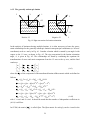
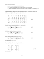
A.1.2 The generally orthotropic lamina
2
Y
1
Y
2
+θ
X
X
−θ
Negative θ
Positive θ
1
Fig. A2 Sign convention for lamina orientation.
In the analysis of laminates having multiple laminae, it is often necessary to know the stressstrain relationships for the generally orthotropic lamina in non-principal coordinates (or 'off-axis'
coordinates) such as x and y in Fig. A1. Consider a lamina which is rotated by an angle θ with
respect to the 1-2 axes, as shown in Fig. A2. The sign convention for the lamina orientation
angle, θ, is given in Fig. A2. The relationships are found by combining the equations for
transformation of stress and strain components from the 12 axes to the xy axes, and the final
results are:
⎧σ x ⎫ ⎡Q11 Q12 Q16 ⎤ ⎧ ε x ⎫
⎪ ⎪ ⎢
⎥⎪ ⎪
(A.9)
⎨σ y ⎬ = ⎢Q12 Q22 Q26 ⎥ ⎨ ε y ⎬
⎪τ ⎪ ⎢Q
⎥⎪ ⎪
⎩ xy ⎭ ⎣ 16 Q26 Q66 ⎦ ⎩γ xy ⎭
where the Qij are the components of the transformed lamina stiffness matrix which are defined as
follows:
Q11 = Q11C 4 + Q22 S 4 + 2(Q12 + 2Q66 ) S 2C 2
Q12 = (Q11 + Q22 − 4Q66 ) S 2C 2 + Q12 (C 4 + S 4 )
Q22 = Q11S 4 + Q22C 4 + 2(Q12 + 2Q66 ) S 2C 2
Q16 = (Q11 − Q12 − 2Q66 )C 3S − (Q22 − Q12 − 2Q66 )CS 3
Q26 = (Q11 − Q12 − 2Q66 )CS 3 − (Q22 − Q12 − 2Q66 )C 3S
Q66 = (Q11 + Q22 − 2Q12 − 2Q66 )C 2 S 2 + Q66 ( S 4 + C 4 )
(A.10)
with C = cosθ and S = sinθ . It should be noted that the number of independent coefficients in
(A.10) is still four.
In CCSM, the matrix [ Qij ] is called Qbar. The Qbar matrix for each ply can be viewed in the
34
More elastic properties form.
The strains can be expressed in terms of the stresses as:
⎧ ε x ⎫ ⎡ S11 S12 S16 ⎤ ⎧σ x ⎫
⎪ ⎪ ⎢
⎥⎪ ⎪
⎨ ε y ⎬ = ⎢ S12 S22 S26 ⎥ ⎨σ y ⎬
⎪γ ⎪ ⎢ S
⎥⎪ ⎪
⎩ xy ⎭ ⎣ 16 S26 S66 ⎦ ⎩τ xy ⎭
(A.11)
where the Sij are the components of the transformed lamina compliance matrix which are defined
by equations similar to, but not exactly the same form as, Eqs. (A.10) (see the reference listed in
A.10 for details).
35
A.2 Classic laminate theory (with bending)
Fig. A3 defines the coordinate system to be used in the description of laminate theory used in
CCSM. The xyz coordinate system is assumed to have its origin on the middle surface of the
plate, so that the middle surface lies in the xy plane. The displacements at a point in the x, y, z
directions are u, v, and w, respectively. The basic assumptions are:
Z
X
Y
Mx
My
Nxy
Nx
Mxy
Nyx
Myx
Ny
Fig. A3 Coordinate system and stress resultants for laminates plate.
1. The plane consists of orthotropic laminae bonded together, with the principal material axes of
the orthotropic laminae oriented along arbitrary directions with respect to the xy axes.
2. The thickness of the plate, t, is small compared to the lengths along the plate edges, a and b.
3. The displacement u, v, and w are small compared with the plate thickness.
4. The in-plane strains ε x , ε y , and γ xy are small compared with unity.
5. Transverse shear strains γ xz and γ yz are neglected.
6. Tangential displacements u and v are linear functions of the through-thickness z coordinate.
7. The transverse normal strain ε x is neglected.
8. Each ply is linear elastic.
9. The plate thickness t is constant.
10. The transverse shear stresses τ xz and τ yz vanish on the plate surfaces defined by z = ± t / 2 .
Assumption 5 is a result of the assumed state of plane stress in each ply, whereas assumptions 5
and 6 together define the Kirchhoff deformation hypothesis that normals to the middle surface
36
remain straight and normal during deformation. According to assumptions 6 and 7, the
displacements can be expressed as:
u = uo (x, y ) + z F1( x, y )
v = v o ( x, y ) + z F2 (x, y )
w = wo ( x, y ) = w(x , y)
(A.12)
where u o and v o are the tangential displacements of the middle surface along the x and y
directions, respectively. Due to assumption 7, the transverse displacement at the middle surface,
wo (x, y ) , is the same as the transverse displacement of any point having the same x and y
coordinates, so w o ( x, y ) = w (x, y) .
Substituting Eqs. (A.12) in the strain-displacement equations for the transverse shear strain and
using assumption 5, we find that
∂u ∂w
∂w
+
= F 1 ( x, y ) +
=0
γ xz =
∂z ∂x
∂x
∂v ∂w
∂w
+
= F 2 ( x, y) +
=0
γ yz =
(A.13)
∂z ∂y
∂y
and that
∂w
∂x
∂w
F2 (x , y) = −
∂y
F 1 ( x, y ) = −
(A.14)
Substituting Eqs. (A.12) and (A.14) in the strain-displacement relations for the in-plane strains,
we find that:
∂u
= ε ox + z κ x
εx =
∂x
∂v
= ε oy + z κ y
εy =
∂y
∂u ∂v
+
= γ oxy + z κ xy
(A.15)
γ xy =
∂y ∂x
where the strains on the middle surface are:
∂u o
∂v o
ε ox =
ε oy =
∂x
∂y
γ oxy =
∂u o ∂v o
+
∂y
∂x
(A.16)
and the curvatures of the middle surface are:
2
2
∂ 2w
∂ w
∂ w
κx = − 2
κy = − 2
κxy = −
(A.17)
∂x∂y
∂y
∂x
Here κ x is the bending curvature associated with bending of the middle surface in the xz plane,
κ y is the bending curvature associated with bending of the middle surface in the yz plane, and
37
κ xy is the twisting curvature associated with out-of-plane twisting of the middle surface, which
lies in the xy plane before deformation.
Since Eqs. (A.15) give the strains at any distance z from the middle surface, the stresses along
arbitrary xy axes in the k-th lamina of a laminate may be found by substituting Eqs. (A.13) into
the lamina stress-strain relationships from Eqs. (A.9) as follows:
⎧σ x ⎫
⎡Q11 Q12 Q16 ⎤ ⎧ ε xo + zκ x ⎫
⎪ ⎪
⎢
⎥ ⎪⎪ o
⎪⎪
⎨σ y ⎬ = ⎢Q12 Q22 Q26 ⎥ ⎨ ε y + zκ y ⎬
⎪τ ⎪
⎪
⎢
⎥ ⎪ o
⎩ xy ⎭k ⎣Q16 Q26 Q66 ⎦ k ⎪⎩γ x + zκ xy ⎪⎭
(A.18)
top
1
2
t
Z(0)
middle surface
Z(2) Z(1)
Z(k-1)
k
t/2
Z(k)
Z(N)
N
Z
bottom
Fig. A4 Laminated plate geometry and ply numbering system.
It is convenient to use forces and moments per unit length in the laminated plate analysis. The
magnitude of these forces may be clear where the geometry of the component is relatively
simple. Where the component is more complex, CCSM should be used as part of a larger
calculation which finds the forces throughout the structure to assess failure of critical sections.
The forces and moments per unit length shown in Fig. A3 are referred to as stress resultants.
The force per unit length in the i-th direction, N i , is given by (i=x, y, z):
t/ 2
⎫
N ⎧ zk
N i = ∫ σ idz = ∑ ⎨ ∫ (σ i ) k dz ⎬
(A.19)
k
=
1
−t/ 2
⎭
⎩z k−1
and the moment per unit length, Mi , is given by:
t/2
⎫
N ⎧ zk
(A.20)
( σ i ) k M i = ∫ σ izdz = ∑ ⎨ ∫ (σ i ) k zdz⎬
k
=
1
−t / 2
⎩z k −1
⎭
38
where t=laminate thickness
( σ i ) k =i-th stress component in the k-th lamina
z k −1 =distance from middle surface to inner surface of the k-th lamina
z k =distance from middle surface to outer surface of the k-th lamina, as shown in Fig. A4
Upon substituting the lamina stress-strain relationships from Eqs. (A.18) in Eqs. (A.19) and
(A.20), respectively, the following relationship is obtained:
⎧ N x ⎫ ⎡ A11
⎪N ⎪ ⎢
⎪ y ⎪ ⎢ A12
⎪⎪ N xy ⎪⎪ ⎢ A16
⎨M ⎬= ⎢
⎪ x ⎪ ⎢ B11
⎪ M y ⎪ ⎢ B12
⎪
⎪ ⎢
⎩⎪M xy ⎭⎪ ⎣⎢ B16
A12
A22
A26
B12
B22
B26
A16
A26
A66
B16
B26
B66
B11
B12
B16
D11
D12
D16
B16 ⎤ ⎧ ε xo ⎫
⎪ ⎪
B26 ⎥⎥ ⎪ ε oy ⎪
o ⎪
B66 ⎥ ⎪⎪γ xy
⎪
⎥⎨ ⎬
D16 ⎥ ⎪ κ x ⎪
D26 ⎥ ⎪ κ y ⎪
⎥⎪ ⎪
D66 ⎦⎥ ⎪κ xy ⎪
⎩ ⎭
B12
B22
B26
D12
D22
D26
(A.21)
where the laminate extensional stiffness, Aij , are given by:
t /2
N
−t / 2
k =1
A ij = ∫ (Qij )k dz = ∑ (Qij )k (z k − z k −1 )
(A.22)
the laminate coupling stiffnesses are given by:
t/2
1 N
Bij = ∫ (Qij ) k zdz = ∑ (Qij ) k (z 2k − z k2 −1 )
2 k =1
−t / 2
(A.23)
and the laminate bending stiffness are given by:
t/2
1 N
Dij = ∫ (Qij )k z 2dz = ∑ (Qij )k (z 3k − z k3 −1 )
3 k =1
−t/ 2
(A.24)
with the subscripts i,j=1,2, or 6.
Equation (A.21) may be written in partitioned form as
o
⎧ N ⎫ ⎡ A M B ⎤ ⎧ε ⎫
⎪ ⎪ ⎢
⎥ ⎪L ⎪
L
L
L
=
⋅
⎨ ⎬ ⎢
⎥⎨ ⎬
⎪M ⎪ ⎢ B M D ⎥ ⎪ κ ⎪
⎩ ⎭ ⎣
⎦⎩ ⎭
(A.25)
for convenience.
39
In CCSM, the stiffness matrix in (A.21) for the laminate is shown in the More Elastic properties
form, by clicking the Laminate Stiffness button.
A.3 Laminate compliances
The inverse of the stiffness matrix (A.21) or (A.25) gives the compliances of the laminate:
⎧ε o ⎫ ⎡ A M B ⎤ −1 ⎧ N ⎫
⎧N ⎫
⎪⎪ ⎪⎪ ⎢
⎪ ⎪
⎪ ⎪
⎥
⎨L ⎬ = ⎢L ⋅ L⎥ ⎨L ⎬ = [S ]⎨L ⎬
(A.26)
⎪ κ ⎪ ⎢ B M D ⎥ ⎪M ⎪
⎪M ⎪
⎦ ⎩ ⎭
⎩ ⎭
⎪⎩ ⎪⎭ ⎣
The above relation is used to calculate the lamina stresses and strains associated with prescribed
laminate loads.
In CCSM, the compliance matrix in (A.26) for laminate is shown in the More Elastic properties
form by clicking the Laminate Compliance button.
For a balanced symmetric laminate, the B sub-matrix is zero, indicating that there is no coupling
between in-plane and bending terms. The upper-left quarter of equation A.26 is now in the same
form as the equivalent equation A3 for an orthotropic lamina. Hence it is appropriate to define
laminate engineering constants Ex, Ey, Gxy νxy and νyx, using the compliance matrix S in equation
A.26, with equivalent expressions to those given in equation A.4, and converting from forces to
stresses via the thickness t;
Ey
Ex
1
1
1
1
1
, Ey =
,
, Gxy =
Ex =
=
=−
=−
(A.27)
tS11
tS 22 ν xy ν yx
tS12
tS 21
tS33
For an unsymmetric matrix, there is coupling between the in-plane and bending terms, so that this
decomposition is no longer valid. However, the compliance matrix S can still give an effective
stiffness where there is only loading in the relevant direction, for example 1/tS11 gives an
effective value for Ex where there is only an Nx load term. These are the values that are quoted.
A.4 Determination of lamina stresses and strains
Calculation of lamina stresses and strains is a straightforward procedure. Making use of Eqs.
(A.9), the stresses in the k-th lamina, when written in abbreviated matrix notation, are given by:
{σ }k
[ ] ({
}
)
= Q k ε o + z{κ }
(A.28)
40
where {ε o} and {κ} are the midplane strains and the curvatures respectively. Here the subscript k
refers to the k-th ply.
A.5 Conventional lamina failure criteria
Five lamina strengths are relevant in the lamina failure analysis. They are:
S(L+ ) : the longitudinal tensile strength
S(L− ) : the longitudinal compressive strength
S(T+ ) : the transverse tensile strength
S(T− ) : the transverse tensile strength
SLT : the in-plane shear strength
A.5.1 Maximum stress
This criterion predicts failure when any principal material axis stress component exceeds the
corresponding strength, i.e. failure occurs whenever one of the following holds:
σ1 ≤ − S (L− )
or
or
σ1 ≥ S (L+ )
σ 2 ≤ − S (T− )
or
σ 2 ≥ S(T+ )
or
τ12 ≥ SLT
(A.29)
The maximum stress in each ply is used in equation A.29 and in corresponding equations for the
other conventional failure criteria (or maximum strain where appropriate). This maximum stress
or strain need not be at the centre of the ply.
A.5.2 Maximum strain
This criterion predicts failure when any principal material axis strain component exceeds the
corresponding ultimate strain, i.e. failure occurs whenever one of the following holds:
ε1 ≤ −e L( −)
or
ε1 ≥ eL( + )
or
ε 2 ≤ −eT( − )
or
ε 2 ≥ eT( + )
or
γ 12 ≥ e LT
(A.30)
41
Assuming linear elastic behaviour, the ultimate strains can be calculated by:
e L( + ) =
S L( + )
( −)
, eL =
E1
S L( −)
E1
(+)
, eT =
ST( + )
E2
( −)
, eT =
ST( −)
E2
, e LT =
S LT
(A.30)
G12
A.5.3 Tsai-Hill
The Tsai-Hill criterion states that failure occurs when the following relation satisfies:
σ 12
S L2
−
σ 1σ 2
S L2
+
σ 22
ST2
+
2
τ 12
2
S LT
≥1
(A.32)
The Tsai-Hill criterion assumes that the material has equal strengths in tension and compression.
When tensile and compressive strengths are different, modification can be made by using the
appropriate value of SL and ST for the corresponding stress components. For example, if σ1 is
(+)
( −)
positive and σ 2 is negative, the values of S L and ST would be used in (A.32).
A.5.4 Tsai-Wu
The Tsai-Wu criterion states that failure occurs when the following relation satisfies:
2
F11σ 12 + F22σ 22 + F66τ 12
+ F1σ 1 + F2σ 2 + 2 F12σ 1σ 2 ≥ 1
(A.33)
where
F11 =
F2 =
1
S L( + ) S L( −)
1
S T( + )
−
F22 =
,
1
ST( −)
,
F66 =
1
S T( + ) S T( − )
1
2
S LT
,
F1 =
,
F12 = −
42
1
−
1
S L( + ) S L( −)
( F11 F22 )1 / 2
2
,
A.6 BFS compressive failure criterion
The unnotched strength of the laminate can be predicted based on either a micromechanics model
or using strength data for each lamina.
The micromechanics model is based on the Budiansky-Fleck compressive failure analysis. In this
section we describe its application to a 0° lamina. Section A.7 explains how this information is used
to find the laminate unnotched strength. This criterion assumes that the unnotched compressive
strength of the lamina is governed by imperfection-sensitive plastic microbuckling with the
imperfection in the form of fibre misalignment. Consider microbuckling from an infinite band of
uniform fibre misalignment φ as shown in Fig. A5 in a unidirectional material. The composite is
subjected to a remote axial stress σL parallel to the fibre direction, an in-plane transverse stress σT
and an in-plane longitudinal shear stress τ. The infinite band is inclined with respect to the fibre axes
such that the normal to the band is rotated by an angle β with respect to the remote fibre direction, as
shown in Fig. A5.
For the case where the composite displays a rigid-perfectly plastic in-plane response the compressive
strength of the lamina is given from Slaughter et al (1993) by
αk − τ − σ T tan β
σL =
(A.34)
φ
2
2
where k is the shear yield strength of the composite and α = 1 + R tan β . The constant R is taken
as 1.5 (Jelf and Fleck 1994).
It may be helpful to review the various input parameters to this model. The dominating influences
are the matrix shear strength and the fibre waviness. The matrix strength k can be estimated from
the yield strength of the unidirectional composite in shear. Typical values for polymer matrices
are in the range 30 - 100 MPa. The estimate of fibre waviness φ is not trivial for real composites
and is the subject of current research. However, a typical value for φ would be in the range of 13° for standard polymer matrix composites. Research suggests that a misaligned region of more
than say 30-50 fibres will be needed to affect the strength; a few misaligned fibres would not
make a difference. Experimentally it is found that microbuckles propagate across the specimen at
a fixed orientation to the direction of the 0 degree fibres. Typically this β angle of propagation of
the microbuckle lies between 20 and 30°. Sutcliffe and Fleck (1997) give theoretical predictions
of the propagation direction. In practice there appears to be little variation in the value of β in
composite materials, and the analysis is not sensitive to this parameter, so that the chosen value
of β is not critical. The review paper by Fleck (1997) gives further details of these microbuckling
models and their inputs.
43
Although the effect of shear stresses have been verified by Jelf and Fleck, the effect of transverse
stresses has not been, and this part of the model should be used with caution. While the analysis
predicts the failure due to plastic microbuckling, the user should also be aware that other modes of
failure may occur; for example elastic microbuckling, splitting, fibre crushing or matrix failure. A
check on the elastic microbuckling limit (equal to G12) is carried out by CCSM, but the user should
be careful in checking that these other modes do not occur. Refer to the work of Jelf and Fleck
(1992) for further information. The B-F model does not allow for plate bending components, and the
stresses at the mid-plane of each ply are used in equation A.34. See Shu and Fleck, 1997, for a
discussion of strain hardening effects, which are not modelled here.
Longitudinal stress
τ
−σ
L
Transverse stress
σ
T
Kink band
inclination
Initial fibre
waviness φ
β
Fig. A5 Infinite band model of microbuckling
The Input Ply Strengths option provides an alternative to the micromechanics model for the
prediction of unnotched laminate strength. This model, as suggested by Soutis and Edge, 1997,
requires as inputs the lamina compressive and shear strengths S L− , and S LT , such as might be
obtained from unidirectional tests. The strength of each ply under combined stresses σ1, σ2 and
τ12 is estimated by linear interpolation, neglecting the transverse stress σ2, so that failure occurs
when
44
− σ1
sL−
+
τ12
≥1
(A.35)
sLT
Only failure of the 0° plies is considered for both the Micromechanical and Ply Strength failure
criteria.
A.7 Laminate failure analysis
The previous two sections discuss several multiaxial failure criteria for estimating the strength of
individual lamina under in-plane stresses. Such criteria can be used on a ply-by-ply basis for a
laminate to determine which ply fails first under in-plane loads. Interlaminar stresses leading to
delamination are not considered in CCSM. For the BFS compressive analysis it is assumed that
failure will occur first in the microbuckling 0° plies. The failure of these 0° lamina is examined
using equation A.34, taking the stresses in the 0° plies arising from the laminate loading. The
laminate strength is given when the stresses on the laminate generates the lamina failure stresses
in a 0° ply.
The prediction of first ply failure due to in-plane stresses is a straightforward application of the
appropriate multiaxial lamina strength criterion in combination with the lamina stress analysis
from the classical lamination theory. Since a laminate generally has plies at several orientations,
the ultimate load-carrying capacity of the laminate may be higher than the first ply failure. The
analysis of subsequent ply failure is not implemented in CCSM.
A.8 Failure of notched laminates
In this section we describe in detail the Fleck-Soutis model used to estimate the notched strength
of laminates. The model assumes that a microbuckle and associated delamination damage grow
from the edge of a sharp notch or hole. The resistance to damage can be modelled using the
unnotched strength and a compressive 'fracture toughness' of the laminate. The unnotched
strength may either be input directly, or the Budiansky-Fleck or ply strength failure criteria
described in section A.6 can be used to predict this. The laminate compressive fracture toughness
Kc, which is derived from the failure load for a panel with a sharp notch, may either be taken
directly from experiments, or it may be predicted from data on laminates of the same material as
that under consideration, but with other lay-ups. Typical values for CFRP composites are in the
range 40 - 50 MPa√m.
45
For countersunk and filled holes, a simple knockdown or strengthening factors of 0.85 and 1.21
respectively are applied, as suggested by Soutis and Edge, 1997. These factors are based on
limited data, and should be used only as guidelines. The equivalent hole is used to model postimpact compressive strength, as described by Soutis and Curtis, 1996. They observe that, when a
panel is loaded in uniaxial compression, damage propagates from regions of delamination (e.g.
arising from impacts) in a similar way to that observed with open holes. Further details, in
particular describing how to estimate the diameter of this equivalent hole, are given in this
reference. The length of the microbuckle at peak load for the equivalent, filled and countersunk
holes may be estimated from the equivalent calculation for an open hole.
Carpet plots, which give the effect of ply mix on notched strength for a symmetric laminate, are
calculated from the data in the failure form for strength, toughness and geometry type. It is
assumed that the composite is composed only of 0, 90 and ±45° plies. Several curves, each
corresponding to a constant proportion of 0° plies, are produced, showing the variation of
strength with the change in ±45° plies. The proportion of 90° plies is found using the fact that the
total proportion of plies sums to 100%. The axial compressive stress is plotted on the graph. The
stress pattern in the failure form is used for these plots. The other stress components will be in the
proportions specified by the load pattern specified here and shown in the Plots form. The
unnotched strength for each ply mix is predicted based on the lamina strength option and
geometry type chosen in the failure form. As for the failure analysis, only failure in the 0 degree
plies is considered. The Soutis-Fleck bridging analysis is used to calculate the notched strength.
The toughness is assumed to be independent of ply mix, and is taken from the Failure Analysis
form. The percentage of 0 degree plies is varied from 10 to 90%. Elastic and strength data for the
first ply are used throughout the laminate. As with the standard BFS compressive failure analysis,
care should be taken in interpreting results at extremes of ply mix, as the BFS compressive
failure criterion may be inappropriate. Soutis and Edge, 1997, give further details of carpet plot
calculations.
In the rest of this section, the details of the method used to calculate the notched strength are
outlined. The method involves crack bridging models, which have had notable success in the
prediction of damage from notches in engineering materials under remote tension. They have also
been used to estimate the development of microbuckling from a hole in a composite under
compression. The usual strategy is to concentrate the inelastic deformation associated with
plasticity, cracking, microbuckling and so on within a crack and to assume some form of tractiondisplacement bridging law across the crack faces. As a simple example, in Dugdale's analysis of
plastic yielding in metals from the root of a notch the bridging normal traction across the crack
faces is assumed to equal the tensile yield strength of the solid. The material response elsewhere
46
in the cracked specimen or structure is assumed to be linear elastic. Other sophisticated examples
adopt more realistic, consequently more complicated, bridging laws. One such example is the
bridging law derived from an infinite band calculation of fibre microbuckling: the crack traction
T versus crack overlap 2v law is assumed to equal the remote stress σ r versus extra remote
displacement Δv response of an infinite microbuckle band under remote compression (the extra
remote displacement is the end shortening minus the contribution to shortening associated with
elastic axial straining).
Details about the bridging analysis, which is incorporated in the current version of CCSM, can be
found in Sutcliffe and Fleck's (1993) paper. Only a brief outline is given below. Although the
effect of compressive loading has been well tested experimentally (e.g. Soutis et al, 1993, Soutis
and Edge, 1997), recent work by Fleck, Liu and Shu, 1998, suggest that the predicted effects of
transverse and shear loading should be treated with caution for notched geometries.
Considered the geometries shown in Fig. A6. The stress intensity factor K σ due to a distribution
of normal compressive stresses σ (x) along the microbuckle at the tip of a microbuckle of length
l is given by the integral:
l
Kσ = ∫ σ ( x ) m(l, x )dx
(A.36)
0
where the weight function m( l , x) can be conveniently found from the point load solution given
by published results for a crack emanating from a central hole and for a single edge notch and a
centre notched panel, which are the three geometries dealt with in the current version of CCSM.
Using the weight function method, the crack closing displacement u σ (x) on the microbuckle face
(where u is half the relative displacement of the two faces of the microbuckle) due to σ(x) is
given by:
uσ ( x ) = −
l'
1 l
m(l' , x ′)dl σ ( x' )m( x, x ′)dx ′
E′ o
0
∫
∫
(A.37)
where the orthotropic equivalent elastic modulus E' is defined by:
1 ⎛⎜
1
=
E ′ ⎜⎝ 2 E xx E yy
1/ 2 ⎡
⎞
⎟
⎟
⎠
⎛E
⎢⎜ yy
⎢⎜⎝ E xx
⎣
1/ 2
⎞
⎟
⎟
⎠
− ν yx
E yy ⎤
⎥
+
2G xy ⎥
⎦
1/ 2
(A.38)
The weight function method is also used to find the stress intensity factor at the microbuckle tip
K rm and the displacements across the microbuckle u r (x) due to the remote stress for the
notched panels, using Bueckner's rule, briefly, that is (A.36) and (A.37) are used again to
calculated K rm and u r (x) but the traction on the crack faces is that along the crack line for a
47
specimen containing no crack. For specimens with a central hole Newman, 1982, gives the stress
intensity factor at the end of the microbuckle and the displacements due to a remote uniform
stress.
The net stress intensity factor at the microbuckle tip K m and the displacements along the
microbuckle u(x) are then:
K m = K σ + Krm
u(x) = uσ (x) + ur (x)
(A.39)
The compressive traction σ(x) across the microbuckle is related to the closing displacement u(x)
across the microbuckle by a functional relationship. For the current situation, a simple linear
softening law is used:
u
⎧
for 0 ≤ u ≤ u c
σ
⎪1 −
= ⎨ uc
(A.40)
σ un ⎪0
for
u
u
>
c
⎩
where u c is a critical microbuckle overlap displacement. The appropriate value of u c is found
from the measured toughness GIC , using the assumed variation of microbuckle load with
displacement,
GIC =
uc
∫0
2σ (u )du = σ unuc
(A.41)
To solve for the remote stress, the cohesive zone is divided into N elements of equal length. The
traction distribution within the cohesive zone is taken to be piecewise linear, with triangular
distributions of crack face traction with peak value centred on the i-th node. The integrals in
equations (A.36) and (A.37) are calculated numerically at the node points for triangular
distributions of traction of unit magnitude at the N node points. N-1 simultaneous equations
concerning the non-zero displacements at the 1 to N-1 discretised nodes (except the node at the
tip where the displacement is zero) are then obtained. An additional equation is that the stress
intensity factor at the tip of the microbuckle K m due to the remote stress and microbuckle
traction is zero:
Km = 0
therefore the system governing equations are fully decided and solved numerically.
The calculations give a relationship between the microbuckle length and the applied remote
stress. The failure stress is given by the maximum applied stress ; the calculations also give the
corresponding critical microbuckle length lc at the maximum stress. CCSM presents results at
failure in terms of the remote stress σL, the average stress over the unnotched ligament b and the
critical microbuckle length.
48
The bridging analysis used in CCSM does not strictly apply with applied shear and transverse
loads. However an estimate of the failure load under these conditions can be made by using the
notched results for purely compressive loading, with the compressive strength knocked down by
an amount given by a failure analysis for unnotched laminates. This is the approach used in
CCSM.
−σ
−σ
−σ
L
L
L
2w
2w
w
2a
b
a
b
2a
l
l
(b)
SEN
(a)
CEN
b
l
(c)
HOLE
Fig. A6 Geometry of specimens (a) centre notch, (b) single edge notch (c) central hole, and the
definitions of a, b, and w.
In general the bridging analysis can be described by the following functional relationship:
lc
a b
= f( , )
(A.42)
rp
rp rp
σr
rp
= g(
where r p =
a b
, )
rp rp
E ' G IC
2
σ un
=
2
K IC
2
σ un
(A.43)
is the bridging length scale, σun is the unnotched strength of the
laminate, lc is the critical microbuckle length, σL is the remote stress of the notched specimen at
failure, a is the half crack length (CEN), or hole radius (HOLE), or total crack length (SEN) and b
is the ligament length.
Equations (A.42) and (A.43) are the basis for the interpolation and extrapolation for the bridging
analysis in CCSM described in the following section.
49
As noted in Sutcliffe and Fleck's (1993) paper, the weight functions used are for isotropic
materials; they show that errors in using them for the orthotropic materials are not too large.
A.9 Interpolation and extrapolation of the bridging analysis data
A number of bridging analyses have been carried out for three types of commonly used
specimens, a centre-cracked panel (CEN), a single edge cracked panel (SEN) and a plate with a
hole (HOLE), and for a range of crack and ligament sizes (Sutcliffe and Fleck, 1993). Results are
expressed as functions of a / rp and b / rp (where a is the half crack size for CEN, crack size for
2
SEN, and hole radius for HOLE, b is the ligament, r p = ( K c / σ un ) is a characteristic length
scale, Kc is the toughness and σ un the unnotched laminate strength). Dimensionless results for
the variation of the notched strength and critical microbuckle length with a / rp and b / rp
between 10–3 and 10+3 for the three notched geometries1 are stored as look-up tables. Use of a
look-up table is more robust and faster than performing the calculation in real time. The look-up
table files are: CENLENG.DAT, CENSTRE.DAT, SENLENG.DAT, SENSTRE.DAT,
HOLELENG.DAT, and HOLESTRE.DAT. Data in these files should not be changed. If the
geometry to be analysed is located at one of the calculated data grid points, the results will be
retrieved directly from the look-up table. If the geometry to be calculated lies in-between or
outside the grid points an interpolation or extrapolation scheme is used to calculate results from
data at the nearest grid points. The rest of this section explains in detail the procedures used.
1
Data from the bridging analysis for the hole are only available for b/w<0.25 and (a+lc)/w<0.75. Values for
geometries outside this range have been estimated, by comparison with the asymptotic values and the centre notch
calculations.
50
A.9.1 For points inside the macro grid of the look-up table
(X1L, X2U)
(X1U, X2U)
grid point 3
grid point 4
(X1, X2)
input point to be interpolated
grid point 1
grid point 2
(X1L, X2L)
(X1U, X2L)
Fig. A7 Schematic figure of a unit grid for the bicubic interpolation
A bicubic interpolation is adopted in CCSM. To do a bicubic interpolation within a unit grid
square [( X1L, X 2L ), ( X1U, X2 L ), ( X1U, X2U ), ( X1L, X2 U )] (see Fig. A7). The function Y and
the derivatives
∂Y
∂Y
∂ 2Y
,
,
at each of the four corners of the square are given in the
∂ X1 ∂ X 2 ∂ X 1∂ X 2
look-up table. The numbering of the corner points starts at the lower left corner, and counts anticlock-wise.
There are two steps to the interpolation, described in detail in the reference listed in A.10: first
obtain the sixteen quantities Cij based on the given functions and its derivatives at the four grid
corners, i, j=1, ..., 4. Next, substitute the C's into the following bicubic interpolation formula for
the point of interest, or the input point, ( X1 , X2 ):
4
Y ( X1, X 2 ) =
4
∑∑ C T
ij
i −1
U
j −1
(A.44)
i =1 j =1
where T =
X 1 − X 1L
X 2 − X 2L
,U=
.
X 1U − X 1L
X 2U − X 2 L
(A.45)
As discussed in the previous section, the bridging analysis can be generally described by the
following functional relationship:
51
lc
a b
= f( , )
rp
rp rp
σr
rp
= g(
(A.46)
a b
, )
rp rp
(A.47)
The bicubic interpolation formula (A.44) is valid for any grid square. Since the precision of the
interpolation will be better for smaller grid sizes, the area of interpolation is divided into smaller
grids and (A.44) is applied to each of these sub-divided grids. To avoid confusion in the
description, we refer to the sub-divided grid as the 'unit grid', while the total area is the 'macro
grid'.
The smoother the function over the grid, the better is the precision of the bicubic interpolation.
When the functions (A.46) and (A.47) are plotted with log axes for a / rp and b / rp , they are
smooth. Therefore the interpolation is carried out in the log(a / r p ) - log(b / r p ) space rather than
as a function of a / rp and b / rp .
For the three types of specimens, the macro grid covers the following unit grid points: log(a/rp)
and log(b/rp)=–3 to 3.
Function values of (A.46) and (A.47) (f and g), together with their corresponding first order
∂f
∂f
,
,
partial
derivatives
and
cross
derivative,
i.e.
∂ log(a / rp )
∂ log(b / r p )
∂2f
∂ 2g
∂g
∂g
and
,
,
at the unit
∂ log(a / r p )∂ log(b / r p )
∂ log(a / rp ) ∂ log(b / rp ) ∂ log(a / r p )∂ log(b / r p )
grid points have been calculated and tabulated in data files. These data files are:
CENLENG.DAT (f and its derivatives for CEN specimen)
CENSTRE.DAT (g and its derivatives for CEN specimen)
SENLENG.DAT (f and its derivatives for SEN specimen)
SENSTRE.DAT (g and its derivatives for SEN specimen)
HOLELENG.DAT (f and its derivatives for HOLE specimen)
HOLESTRE.DAT (g and its derivatives for HOLE specimen)
In the CCSM bridging analysis if the input data point log(a / r p ) – log(b / r p ) is within the lower
and upper bounds of the macro grid, the program will find the right unit grid square which
encloses the input data point ( a / r p , b / r p ) and the function values for the remote stress σr and
the critical microbuckle length lc at the input point will be interpolated from the unit grid using
52
the bicubic interpolation (A.44).
A.9.2 For points outside the macro grid of the look-up table
When the input data point falls outside the macro grid, an extrapolation technique has to be used.
CCSM relies on the asymptotic nature of the solution in these areas to obtain the correct values.
Details are given in the references quoted. Three distinct regions are noted:
Region (1): when a / rp , b / rp are both very large, loading is in the so-called LEFM situation
where the remote applied stress intensity factor at failure will be equal to the fracture toughness
of the composite, i.e. K r = Kc , and the microbuckle length is found to be: l c =0.75rp for both
CEN and SEN specimens. The remote stress can then be backed out from the K r value by the
LEFM formula. For the HOLE specimen, failure is determined by the stress concentration factor,
i.e. K tσ r = σ un , while the l c tends to 0 and becomes unstable.
The limits, in summary are:
when
a / r p >> 1 and b / r p >> 1
CEN:
Kr → Kc
l c → 0.75rp
SEN:
HOLE:
σ r = K r /(Y πa )
(A.48)
σ r = K r /(Y πa )
(A.49)
Kr → Kc
l c → 0.75rp
l c → 0 (unstable)
σ r = σ un / K t (K t is the stress concentration factor)
53
(A.50)
Region (2): when a / r p is small and b / r p large, the situation is summarised below:
when
a / r p << 1 and b / r p >> 1
CEN:
l c → 0.45r p
σ r → σ un b / w
SEN:
K r = Yσ r πa
l c → 0 .4 r p
(A.51)
σr →σun(b / w)2
HOLE:
K r = Yσ r πa
l c → 0.55r p
(A.52)
σ r → σ un b / w
(A.53)
Region (3): when b / r p is very small (regardless of the value of a / r p ), we find:
when
b / r p << 1
CEN:
lc → b
σ r → σ un b / w
SEN:
K r = Yσ r πa
lc → b
(A.54)
σ r → σ un (b / w) 2
HOLE:
K r = Yσ r πa
lc → b
σ r → σ un b / w
(A.55)
(A.56)
In the actual calculation, the above asymptotic solutions are assumed to be reached when
log(a/rp)) or log(b/rp) = ±3.
While there are asymptotic solutions in certain areas outside the interpolation grid, in other areas
there is a transition between two types of asymptotic behaviour. The way in which CCSM
handles data in this area is explained by way of example.
Consider a centre notched specimen with small a/rp; there is a transition from LEFM with failure
determined by a stress intensity factor criterion, to failure given by the unnotched strength, as
b/rp changes from being very large to very small. In the extrapolation scheme, it is assumed that
the form of the transition is not dependent on the value of a/rp in this area, as long as a/rp remains
small, and varies in the following way with b/rp
54
σr
= g1(B) = λ (B) (w1 lim1(B) + w2 lim 2 (B))
σ un
⎛
⎛ b ⎞⎞
⎛ (B + 3)π ⎞
and w1 + w 2 = 1
where B = ⎜ log10 ⎜ ⎟ ⎟ , w1 = 0.5 + 0.5cos
⎝
⎠
6
⎝ rp ⎠ ⎠
⎝
(A.57)
where the functions lim1 and lim2 are the expressions for the stress or stress intensity factor K
which apply asymptotically at either end of the boundary of the calculated grid with b/rp small
and large respectively (in this case they would be given by equations A.54 and A.51). λ, which is
a function of b/rp , expresses the form of the transition in behaviour between these extremes, and
is found from the data computed at the edge of the grid (along a/rp = 0.001 in this case).
Similar expressions are used along any other boundaries where there is a transition in limiting
behaviour.
B.10 References
References for each of the above theory sections are given below.
Sections B.1
to B.5, B.7
and B.10:
Section B.6:
R. F. Gibson, Principles of Composite Material Mechanics, McGrawHill, 1994
Sections B.8 and
B.9
M. P. F. Sutcliffe and N. A. Fleck, Effect of geometry upon
compressive failure of notched composites, Int. J. Fracture, 59,
pp.115-132, 1993
B. Budiansky and N. A. Fleck, Compressive failure of fibre
composites, J. Mech. Phys. Solids, 41(1), pp.183-211, 1993
B. N. Cox and D. B. Marshall, Acta Metall. et Mater., 39, 59-589,
1991
J. C. Newman, in Proceedings of the AGARD Conference on the
Behaviour of Short Cracks in Airframe Components, France, 1982
Section B.9
W. H. Press, S. A. Teukolsky, W. T. Vetterling and B. P. Flannery,
Numerical Recipes in FORTRAN, Second Edition, Cambridge
University Press, 1994
55
Other references and further reading
B. Budiansky and N. A. Fleck, (1994) Compressive kinking of fiber composites: a topical review,
Appl. Mech. Rev., 47(6), part 2, S246-S250W.
B. Budiansky and N. A. Fleck, (1993) Compressive failure of fibre composites, J. Mech. Phys.
Solids, 41(1), pp.183-211
B. N. Cox and D. B. Marshall, (1991) Acta Metall. et Mater., 39, 59-589
N. A. Fleck, L. Deng and B. Budiansky, (1995) Prediction of kind band width in fiber
composites, J. Applied Mech 62, pp329-337
NA Fleck (1997) "Compressive Failure of Fibre Composites" Advances in Applied Mechanics,
Vol. 34, Academic Press, ed. JW Hutchinson and TY Wu, pp 43-118
NA Fleck, D Liu and JY Shu (1998) Microbuckle initiation from a hole and from the free edge of
a fibre composite' submitted to Int J Solids and Structures
R. F. Gibson, (1994) Principles of Composite Material Mechanics, McGraw-Hill,
P. M. Jelf and N. A. Fleck (1992) Compression failure mechanisms in unidirectional composites.
Journal of Composite Materials 26 2706-2726
P. M. Jelf and N. A. Fleck (1994) The failure of composite tubes due to combined compression
and torsion. J. Materials Science 29 3080-3086
J. C. Newman, (1982) in Proceedings of the AGARD Conference on the Behaviour of Short
Cracks in Airframe Components, France
W. H. Press, S. A. Teukolsky, W. T. Vetterling and B. P. Flannery, (1994) Numerical Recipes in
FORTRAN, Second Edition, Cambridge University Press
JY Shu and NA Fleck (1997) Microbuckle initiation in fibre composites under multiaxial
loading', Proc Roy Soc A453, 2063-2083
S. Slaughter, N. A. Fleck and B. Budiansky, (1992) Microbuckling of fibre composites: the role
of multi-axial loading and creep, J. Eng. Mater. Tech., 115(5), pp.308-313.
C. Soutis, N.A. Fleck and P.A. Smith (1991) Failure prediction technique for compression loaded
carbon fibre-epoxy laminate with open holes, J Comp. Materials, 25, 1476-1498.
C Soutis, PT Curtis and NA Fleck (1993) "Compressive failure of notched carbon fibre
composites" Proc R. Soc. London A, Vol. 440, pp 241-256
C Soutis and PT Curtis (1996) "Prediction of the post-impact compressive strength of CFRP
laminated composites", Composites Science and Technology, 56, pp 677-684.
C. Soutis and EC Edge (1997), A method for the production of carpet plots for notched
compression strength of carbon fibre reinforced plastic multidirectional laminates, Proc Instn
Mech Engrs, 211 (G), pp 251-261
M. P. F. Sutcliffe and N. A. Fleck, (1993), Effect of geometry upon compressive failure of
notched composites, Int. J. Fracture, 59, pp.115-132
MPF Sutcliffe and NA Fleck (1997) "Microbuckle propagation in fibre composites" Acta
Metallurgica and Materialia, , pp921-932
56