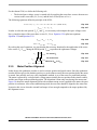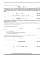
Download DRM105, PM Sinusoidal Motor Vector Control with Quadrature

PM Sinusoidal Motor Vector Control
with Quadrature Encoder
Designer Reference Manual
Devices Supported:
MCF51AC256
Document Number: DRM105
Rev. 0
09/2008
How to Reach Us:
Home Page:
www.freescale.com
Web Support:
http://www.freescale.com/support
USA/Europe or Locations Not Listed:
Freescale Semiconductor, Inc.
Technical Information Center, EL516
2100 East Elliot Road
Tempe, Arizona 85284
1-800-521-6274 or +1-480-768-2130
www.freescale.com/support
Europe, Middle East, and Africa:
Freescale Halbleiter Deutschland GmbH
Technical Information Center
Schatzbogen 7
81829 Muenchen, Germany
+44 1296 380 456 (English)
+46 8 52200080 (English)
+49 89 92103 559 (German)
+33 1 69 35 48 48 (French)
www.freescale.com/support
Japan:
Freescale Semiconductor Japan Ltd.
Headquarters
ARCO Tower 15F
1-8-1, Shimo-Meguro, Meguro-ku,
Tokyo 153-0064
Japan
0120 191014 or +81 3 5437 9125
[email protected]
Asia/Pacific:
Freescale Semiconductor China Ltd.
Exchange Building 23F
No. 118 Jianguo Road
Chaoyang District
Beijing 100022
China
+86 10 5879 8000
[email protected]
Freescale Semiconductor Literature Distribution Center
P.O. Box 5405
Denver, Colorado 80217
1-800-441-2447 or +1-303-675-2140
Fax: +1-303-675-2150
[email protected]
Information in this document is provided solely to enable system and
software implementers to use Freescale Semiconductor products. There are
no express or implied copyright licenses granted hereunder to design or
fabricate any integrated circuits or integrated circuits based on the
information in this document.
Freescale Semiconductor reserves the right to make changes without further
notice to any products herein. Freescale Semiconductor makes no warranty,
representation or guarantee regarding the suitability of its products for any
particular purpose, nor does Freescale Semiconductor assume any liability
arising out of the application or use of any product or circuit, and specifically
disclaims any and all liability, including without limitation consequential or
incidental damages. “Typical” parameters that may be provided in Freescale
Semiconductor data sheets and/or specifications can and do vary in different
applications and actual performance may vary over time. All operating
parameters, including “Typicals”, must be validated for each customer
application by customer’s technical experts. Freescale Semiconductor does
not convey any license under its patent rights nor the rights of others.
Freescale Semiconductor products are not designed, intended, or authorized
for use as components in systems intended for surgical implant into the body,
or other applications intended to support or sustain life, or for any other
application in which the failure of the Freescale Semiconductor product could
create a situation where personal injury or death may occur. Should Buyer
purchase or use Freescale Semiconductor products for any such unintended
or unauthorized application, Buyer shall indemnify and hold Freescale
Semiconductor and its officers, employees, subsidiaries, affiliates, and
distributors harmless against all claims, costs, damages, and expenses, and
reasonable attorney fees arising out of, directly or indirectly, any claim of
personal injury or death associated with such unintended or unauthorized
use, even if such claim alleges that Freescale Semiconductor was negligent
regarding the design or manufacture of the part.
Freescale™ and the Freescale logo are trademarks of Freescale
Semiconductor, Inc. All other product or service names are the property of their
respective owners.
© Freescale Semiconductor, Inc. 2008. All rights reserved.
DRM105
Rev. 0
09/2008
Chapter 1
Introduction
1.1
1.2
1.3
Introduction . . . . . . . . . . . . . . . . . . . . . . . . . . . . . . . . . . . . . . . . . . . . . . . . . . . . . .
1.1.1 Application Features and Components . . . . . . . . . . . . . . . . . . . . . . . . . . .
1.1.2 Sinusoidal PM Synchronous Motors Applications Overview . . . . . . . . . .
Freescale Controller Advantages and Features . . . . . . . . . . . . . . . . . . . . . . . . . .
Bibliography . . . . . . . . . . . . . . . . . . . . . . . . . . . . . . . . . . . . . . . . . . . . . . . . . . . . . .
1.3.1 Acronyms and Abbreviations . . . . . . . . . . . . . . . . . . . . . . . . . . . . . . . . . .
1.3.2 Glossary of Terms . . . . . . . . . . . . . . . . . . . . . . . . . . . . . . . . . . . . . . . . . . .
1.3.3 Glossary of Symbols . . . . . . . . . . . . . . . . . . . . . . . . . . . . . . . . . . . . . . . . .
3
3
3
4
6
7
7
8
Chapter 2
Control Theory
2.1
2.2
2.3
3-Phase PM Synchronous Motor . . . . . . . . . . . . . . . . . . . . . . . . . . . . . . . . . . . . .
Mathematical Description of PM Synchronous Motors . . . . . . . . . . . . . . . . . . . .
2.2.1 Space Vector Definitions . . . . . . . . . . . . . . . . . . . . . . . . . . . . . . . . . . . . .
2.2.2 PM Synchronous Motor Model . . . . . . . . . . . . . . . . . . . . . . . . . . . . . . . .
Vector Control of PM Synchronous Motor . . . . . . . . . . . . . . . . . . . . . . . . . . . . . .
2.3.1 Fundamental Principle of Vector Control . . . . . . . . . . . . . . . . . . . . . . . .
2.3.2 Description of the Vector Control Algorithm . . . . . . . . . . . . . . . . . . . . . .
2.3.3 Stator Voltage Decoupling . . . . . . . . . . . . . . . . . . . . . . . . . . . . . . . . . . .
2.3.4 Space Vector Modulation . . . . . . . . . . . . . . . . . . . . . . . . . . . . . . . . . . . .
2.3.5 Motor Position Alignment . . . . . . . . . . . . . . . . . . . . . . . . . . . . . . . . . . . .
11
11
12
13
15
15
16
17
18
21
Chapter 3
System Concept
3.1
3.2
3.3
System Specification . . . . . . . . . . . . . . . . . . . . . . . . . . . . . . . . . . . . . . . . . . . . . . 23
Application Description . . . . . . . . . . . . . . . . . . . . . . . . . . . . . . . . . . . . . . . . . . . . 23
Control Process . . . . . . . . . . . . . . . . . . . . . . . . . . . . . . . . . . . . . . . . . . . . . . . . . . 24
Chapter 4
Hardware
4.1
4.2
4.3
Hardware Implementation . . . . . . . . . . . . . . . . . . . . . . . . . . . . . . . . . . . . . . . . . . 27
3-phase Motor Control Drive using MCF51AC256 . . . . . . . . . . . . . . . . . . . . . . . 29
Motor Specifications — Example . . . . . . . . . . . . . . . . . . . . . . . . . . . . . . . . . . . . . 31
Chapter 5
Software Design
5.1
5.2
Introduction . . . . . . . . . . . . . . . . . . . . . . . . . . . . . . . . . . . . . . . . . . . . . . . . . . . . .
Application Variables Scaling . . . . . . . . . . . . . . . . . . . . . . . . . . . . . . . . . . . . . . . .
5.2.1 Fractional Numbers Representation . . . . . . . . . . . . . . . . . . . . . . . . . . . .
5.2.2 Scaling of Analog Quantities . . . . . . . . . . . . . . . . . . . . . . . . . . . . . . . . . .
5.2.3 Scaling of Angles . . . . . . . . . . . . . . . . . . . . . . . . . . . . . . . . . . . . . . . . . .
33
33
33
33
34
PM Sinusoidal Motor Vector Control with Quadrature Encoder, Rev.0
Freescale Semiconductor
1
5.3
5.4
5.5
5.6
5.2.4 Scaling of Parameters . . . . . . . . . . . . . . . . . . . . . . . . . . . . . . . . . . . . . . .
Application Overview . . . . . . . . . . . . . . . . . . . . . . . . . . . . . . . . . . . . . . . . . . . . . .
5.3.1 ADC Conversion Timing and PWM Reload Interrupts . . . . . . . . . . . . . .
5.3.2 3-Phase Current Sampling . . . . . . . . . . . . . . . . . . . . . . . . . . . . . . . . . . .
5.3.3 Position and Speed Sensing Using Encoder . . . . . . . . . . . . . . . . . . . . .
Transition between the Modes . . . . . . . . . . . . . . . . . . . . . . . . . . . . . . . . . . . . . . .
Software Implementation . . . . . . . . . . . . . . . . . . . . . . . . . . . . . . . . . . . . . . . . . . .
5.5.1 Software States . . . . . . . . . . . . . . . . . . . . . . . . . . . . . . . . . . . . . . . . . . .
5.5.2 Initialization . . . . . . . . . . . . . . . . . . . . . . . . . . . . . . . . . . . . . . . . . . . . . . .
5.5.3 Application Background Loop . . . . . . . . . . . . . . . . . . . . . . . . . . . . . . . . .
5.5.4 Interrupts . . . . . . . . . . . . . . . . . . . . . . . . . . . . . . . . . . . . . . . . . . . . . . . .
5.5.5 FTM1 Overflow Interrupt . . . . . . . . . . . . . . . . . . . . . . . . . . . . . . . . . . . . .
5.5.6 PI Controller Parameters . . . . . . . . . . . . . . . . . . . . . . . . . . . . . . . . . . . .
FreeMASTER Software . . . . . . . . . . . . . . . . . . . . . . . . . . . . . . . . . . . . . . . . . . . .
5.6.1 FreeMASTER Serial Communication Driver . . . . . . . . . . . . . . . . . . . . . .
5.6.2 FreeMASTER Recorder . . . . . . . . . . . . . . . . . . . . . . . . . . . . . . . . . . . . .
5.6.3 FreeMASTER Control Page . . . . . . . . . . . . . . . . . . . . . . . . . . . . . . . . . .
34
36
37
38
39
45
46
47
49
51
51
53
53
53
54
55
55
Chapter 6
Application Setup
6.1
6.2
3-phase Motor Control Drive using MCF51AC256 Setup . . . . . . . . . . . . . . . . . . 57
Demo Hardware Setup . . . . . . . . . . . . . . . . . . . . . . . . . . . . . . . . . . . . . . . . . . . . 58
Chapter 7
Results and Measurements
7.1
7.2
System and Measurement Conditions . . . . . . . . . . . . . . . . . . . . . . . . . . . . . . . . .
7.1.1 Hardware Setup . . . . . . . . . . . . . . . . . . . . . . . . . . . . . . . . . . . . . . . . . . .
7.1.2 Software Setup . . . . . . . . . . . . . . . . . . . . . . . . . . . . . . . . . . . . . . . . . . . .
7.1.3 FreeMASTER . . . . . . . . . . . . . . . . . . . . . . . . . . . . . . . . . . . . . . . . . . . . .
Measured Results . . . . . . . . . . . . . . . . . . . . . . . . . . . . . . . . . . . . . . . . . . . . . . . .
7.2.1 3-Phase Current Reconstruction . . . . . . . . . . . . . . . . . . . . . . . . . . . . . .
7.2.2 Speed Controller . . . . . . . . . . . . . . . . . . . . . . . . . . . . . . . . . . . . . . . . . . .
7.2.3 Current Controller . . . . . . . . . . . . . . . . . . . . . . . . . . . . . . . . . . . . . . . . . .
61
61
61
61
61
61
62
63
PM Sinusoidal Motor Vector Control with Quadrature Encoder, Rev.0
2
Freescale Semiconductor
Chapter 1
Introduction
1.1
Introduction
This paper describes the design of a 3-phase PMSM vector control drive with 3-shunt current sensing using
a quadrature encoder as a position and speed sensor. The design is targeted at consumer and industrial
applications. This cost-effective solution benefits from the Freescale Semiconductor MCF51AC256
device, dedicated for motor control.
1.1.1
Application Features and Components
The system is designed to drive a 3-phase PM synchronous motor. Application features:
• It implements three-phase PMSM speed vector (FOC) control using quadrature encoder.
• It has current sensing with three current sensors.
• Design is based on Freescale MCF51AC256 controller.
• Application is running on a 3-phase Motor Control Drive (12 V) board with an MCFAC51AC256
daughter board.
• Works with FreeMASTER software control interface and monitor.
Main application components available to customers are:
• Software — written in C-code using some library algorithms — available for the MCF51AC256
• Hardware — based on Freescale universal motor control hardware modules
• Documentation — this document
1.1.2
Sinusoidal PM Synchronous Motors Applications Overview
Sinusoidal PM synchronous motors are more and more popular for new drives, replacing brushed DC,
universal, and other motors in a wide application area. The reason is better reliability (no brushes), better
efficiency, lower acoustic noise, and also other benefits of electronic control. A disadvantage of PM
synchronous motor drives is the need for a more sophisticated electronic circuit. But nowadays, most
applications need electronic speed or torque regulation and other features that require electronic control.
When we use a system with electronic control, it is only a small system cost increase to implement more
advanced drives like the sinusoidal PM synchronous motor with digitally controlled switching inverter and
a DC-bus circuit. It is necessary to have a cost-effective controller with good calculation performance. One
of them is Freescale’s MCF51AC256.
The PM synchronous motor has advantages when compared to an AC induction motor. Since a PM
synchronous motor achieves higher efficiency by generating the rotor magnetic flux with rotor magnets, it
PM Sinusoidal Motor Vector Control with Quadrature Encoder, Rev.0
Freescale Semiconductor
3
is used in white goods (such as refrigerators, washing machines, dishwashers), pumps, fans, and in other
appliances that require high reliability and efficiency.
3-phase synchronous motors with permanent magnets come in two most popular variants: the sinusoidal
PM synchronous motor and the trapezoidal BLDC motor. The sinusoidal PM synchronous motor is very
similar to the trapezoidal BLDC (electronically commuted) motor. There are two main differences:
• Motor construction
— The shape of BEMF inducted voltage — sinusoidal (PM synchronous motor) versus
trapezoidal (BLDC) motor
• Control — shape of the control voltage
— 3-phase sinusoidal (all three phases connected at one time) versus rectangular six-step
commutation (one phase is non-conducting at any time)
Generally, we can say that the sinusoidal PM synchronous motor performance is better due to constant
torque, while the trapezoidal BLDC motor can be more easily controlled. The trapezoidal BLDC motors
are used mainly for historical reasons. It was easier to create a six-step commutation and estimate the rotor
position with simpler algorithms, since one phase is non-conducting. The sinusoidal PM synchronous
motors require more sophisticated control, but give us some benefits, such as smoother torque, lower
acoustic noise, and so on. As shown in this document, the MCF51AC256 provides all the necessary
functionality for 3-phase sinusoidal PM synchronous motor vector control. Using the MCF51AC256, we
have a strong argument to replace the trapezoidal BLDC (electronically commuted) motors with the
3-phase sinusoidal PM synchronous motors with almost no system cost increase.
The application described here is a speed vector control. The speed control algorithms can be sorted into
two general groups. The first group applies to scalar control. The constant volt per hertz control is a very
popular technique used for representing scalar control. The other group is called vector-oriented or
field-oriented control (FOC). The vector-oriented techniques bring overall improvements to drive
performance over scalar control. Among them are higher efficiency, full torque control, decoupled control
of flux and torque, improved dynamics, and so on.
For the PM synchronous motor control, it is necessary to know the exact rotor position. The quadrature
encoder is used as a speed and position sensor in this application.
This reference design manual describes the basic motor theory, the system design concept, hardware
implementation and software design, including the FreeMASTER software visualization tool.
1.2
Freescale Controller Advantages and Features
Freescale’s MCF51AC256 is well suited for digital motor control, combining calculation capability with
the MCU’s controller features in a single chip. These controllers offer many dedicated peripherals, such as
pulse width modulation (FTM) modules, analog-to-digital converters (ADC), timers, communication
peripherals (SCI, SPI, I2C), and on-board flash and RAM.
The MCF51AC256 provides the following peripheral blocks:
• Two FTM modules with PWM outputs, fault input, fault-tolerant design with dead time insertion,
supporting both center-aligned and edge-aligned modes
• 12-bit ADC; ADC and PWM modules can be synchronized
PM Sinusoidal Motor Vector Control with Quadrature Encoder, Rev.0
4
Freescale Semiconductor
•
•
•
•
•
•
•
•
•
•
•
•
•
•
•
•
•
•
One two-input 16-bit general purpose timer module
Two serial peripheral interfaces (SPI)
Two serial communications interfaces (SCI) with LIN slave functionality
One inter-integrated circuit (I2C) port
On-board 5.0 V to 2.7 V voltage regulator for powering internal logic and memories
Integrated power-on reset and low-voltage interrupt module
All pins multiplexed with general purpose input/output (GPIO) pins
Computer operating properly (COP) watchdog timer
Two analog comparators
One real-time counter (RTC)
One programmable interval timer (PIT)
External reset input pin for hardware reset
msCAN interface for industrial control
Low-voltage detect (LVD), low-voltage warning (LVW)
Multi-clock generator (MCG)
IEC60730 class C safety features
On-chip ICE and BDM
Phase-locked loop (PLL) based frequency synthesizer for the controller core clock, with on-chip
relaxation oscillator
Table 1-1. Memory Configuration
Memory Type
MCF51AC256
Program Flash
256 KB
Unified Data/Program RAM
32 KB
The PMSM vector control benefits greatly from the FlexTimer (FTM) module, ADC, and timer (TPM)
modules.
The FTM offers flexibility in its configuration, enabling efficient 3-phase motor control. The FTM module
is capable of generating asymmetric PWM duty cycles in center-aligned configuration.
The FTM block has the following features:
• Three complementary PWM signal pairs, or six independent PWM signals (or a combination)
• Complementary channel operation features
• Dead time insertion
• Separate top and bottom polarity control
• Clock source up to two times the bus clock
• Edge-aligned or center-aligned PWM reference signals
• 16-bit resolution
• Mask/swap capability
PM Sinusoidal Motor Vector Control with Quadrature Encoder, Rev.0
Freescale Semiconductor
5
•
•
•
•
Programmable fault protection
Polarity control
Write-protectable registers
Trigger event generation for the ADC module (only in complementary mode when channel three
or five is free)
The ADC module has the following features:
• 12-bit resolution
• 28 inputs
• Hardware trigger
• Input clock selectable from up to four sources
• 2.5 µs per sample conversion
• Interrupt-generating capabilities when the sample is converted
The application uses the ADC block, synchronized to the PWM pulses. This configuration allows the
simultaneous conversion of the required analog values for the inverter currents and DC-bus voltage within
the required time.
The TPM is an extremely flexible module, providing all required services relating to time events. It has the
following features:
• Two 16-bit counters/timers
• Programmable count modulus
• Maximum count rate equal to the bus clock, when counting events
• Can count once or repeatedly
• Counters can share available input pins
• Each counter has a separate prescaler
• Each counter has capture and compare capability
• External timer clock source input pin
The application uses the two channels of the TPM for quadrature encoder signals decoding.
1.3
Bibliography
1. MCF51AC256 ColdFire® Integrated Microcontroller Reference Manual, Freescale
Semiconductor, 2007
2. ColdFire® Family Programmer’s Reference Manual, Freescale Semiconductor, 2005
3. CodeWarrior™ Development Studio 8/16-Bit IDE User’s Guide, Freescale Semiconductor, 2007
4. 3-Phase Motor Control Drive Board User’s Manual, Freescale Semiconductor, 2008
5. MCF51AC256 Daughter Board User’s Manual, Freescale Semiconductor, 2008
6. FreeMASTER Software Users Manual, Freescale Semiconductor, 2004
7. 3-Phase PM Synchronous Motor Vector Control using DSP56F80x, by Prokop L., Grasblum P.,
AN1931 Motorola, 2002
PM Sinusoidal Motor Vector Control with Quadrature Encoder, Rev.0
6
Freescale Semiconductor
For a current list of documentation, refer to www.freescale.com.
1.3.1
Acronyms and Abbreviations
Table 1-2 contains sample acronyms and abbreviations used in this document.
Table 1-2. Acronyms and Abbreviated Terms
Term
Meaning
AC
Alternating current
ADC
Analog-to-digital converter
FTM
FlexTimer module
TPM
Timer module
BEMF
Back electromagnetic force = induced voltage
BLDC
Brushless direct current motor
COP
Computer operating properly (watchdog timer)
DC
Direct current
DSC
Digital signal controller
DT
Dead time: a short time that must be inserted between the turning off of one transistor in the inverter half
bridge and turning on of the complementary transistor due to limited switching speed of the transistors
FOC
Field oriented control
GPIO
General purpose input/output
I/O
Input/output interfaces between a computer system and the external world (A CPU reads an input to sense
the level of an external signal and writes to an output to change the level of an external signal)
BDM
Background debug module
LED
Light emitting diode
MCF51AC256
PI controller
PLL
Freescale ColdFireV1 32-bit controller
Proportional-integral controller
Phase-locked loop: a clock generator circuit in which a voltage controlled oscillator produces an oscillation
that is synchronized to a reference signal
PMSM
PM Synchronous Motor, permanent magnet synchronous motor
PWM
Pulse width modulation
RPM
Revolutions per minute
SCI
Serial communication interface module: a module that supports asynchronous communication
1.3.2
Glossary of Terms
Table 1-3 shows a glossary of terms used in this document.
PM Sinusoidal Motor Vector Control with Quadrature Encoder, Rev.0
Freescale Semiconductor
7
Table 1-3. Glossary
Term
Definition
brush
A component transferring electrical power, from non-rotational terminals mounted on the stator, to the rotor.
commutator
A mechanical device alternating DC current in a DC commutator motor and providing rotation of DC commutator
motor.
duty cycle
The ratio of the amount of time the signal is on to the time it is off. Duty cycle is usually quoted as a percentage.
Quadrature
Encoder
A position sensor giving two code tracks with sector positioned 90 degrees out of phase. The two output
channels indicate both the position and the direction of motor rotation.
interrupt
A temporary break in the sequential execution of a program to respond to signals from peripheral devices by
executing a subroutine.
PM
Synchronous
Motor
Permanent magnet synchronous motor
PI controller
Proportional-integral controller
Quick Start
SW set of algorithms and drivers including Graphical Configuration Tool for DSC/CPU initialization.
reset
To force a device to a known condition.
software
Instructions and data that control the operation of a microcontroller.
1.3.3
Glossary of Symbols
Table 1-4 shows a glossary of symbols used in this document.
Table 1-4. Glossary of Symbols
Term
Definition
d,q
Rotational orthogonal coordinate system
d,q*, (d,q)*
Rotational orthogonal coordinate system estimated coordinates
eSd,q , eS(d,q)
BEMF (induced voltage) in d,q coordinate system
eSα,β , eS(α,β)
BEMF (induced voltage) in α,β coordinate system
eS0
BEMF at a stand point
êSd,q , êS(d,q)
Estimated BEMF (induced voltage) in d,q coordinate system
êSα,β , êS(α,β)
Estimated BEMF (induced voltage) in α,β coordinate system
E IIêII
Estimated BEMF amplitude
g1
SMO feedback gain real component
g1, g2
To force a device to a known condition
gω
Adaptive speed scheme gain
iSd,q , iS(d,q)
Stator currents in d,q coordinate system
iS(d,q)*
Stator currents in estimated d,q coordinate system
PM Sinusoidal Motor Vector Control with Quadrature Encoder, Rev.0
8
Freescale Semiconductor
Table 1-4. Glossary (Continued)of Symbols
Term
Definition
iSα,β , iS(α,β)
Stator currents in α,β coordinate system
îSα,β , îS(α,β)
Estimated stator currents in a,b coordinate system
îSd,q , îS(d,q)
Estimated stator currents in d,q coordinate system
îS(d,q)*
Estimated stator currents in estimated d,q coordinate system
J
Mechanical inertia
k1
SMO switching gain
KM
Motor constant
Ls
Stator phase inductance
∆Ls
Stator phase inductance error
Lsd
Stator phase inductance d axis
Lsq
Stator phase inductance q axis
pp
Number of poles per phase
Rs
Stator phase resistance
te
Electromagnetic torque
TL
Load torque
uSα,β , uS(α,β)
Stator voltages in a,b coordinate system
uSd,q , uS(d,q)
Stator voltages in d,q coordinate system
α,β
Stator orthogonal coordinate system
ε1(α,β)
Current estimation error in a,b coordinate system
ε2(α,β)
BEMF estimation error in a,b coordinate system
ε1(d,q)
Current estimation error in d,q coordinate system
ε2(d,q)
BEMF estimation error in d,q coordinate system
ε2d
BEMF estimation error d component of d,q coordinate system
ΨSα,β
Stator magnetic fluxes in a,b coordinate system
ΨSd,q
Stator magnetic fluxes in d,q coordinate system
ΨM
Rotor magnetic flux
∆θ
Angle estimation error
∆θmax
Maximal wanted angle estimation error
θr
Rotor position angle in a,b coordinate system
ωel0
Electrical rotor angular speed at a standpoint
ω, ωel/ ωF
Electrical rotor angular speed / fields angular speed
PM Sinusoidal Motor Vector Control with Quadrature Encoder, Rev.0
Freescale Semiconductor
9
PM Sinusoidal Motor Vector Control with Quadrature Encoder, Rev.0
10
Freescale Semiconductor
Chapter 2
Control Theory
2.1
3-Phase PM Synchronous Motor
The PM synchronous motor is a rotating electric machine with classic 3-phase stator like that of an
induction motor; the rotor has surface-mounted permanent magnets (see Figure 2-1).
Stator
Stator winding
(in slots)
Shaft
Rotor
Air gap
Permanent magnets
Figure 2-1. PM Synchronous Motor — Cross Section
In this respect, the PM synchronous motor is an equivalent to an induction motor, where the air gap
magnetic field is produced by a permanent magnet, so the rotor magnetic field is constant. PM synchronous
motors offer a number of advantages in designing modern motion-control systems. The use of a permanent
magnet to generate substantial air gap magnetic flux makes it possible to design highly efficient PM
motors.
2.2
Mathematical Description of PM Synchronous Motors
There are a number of PM synchronous motor models. The model used for vector control design can be
obtained by utilizing space-vector theory. The 3-phase motor quantities (such as voltages, currents,
magnetic flux, and so on), are expressed in terms of complex space vectors. Such a model is valid for any
instantaneous variation of voltage and current, and adequately describes the performance of the machine
under both steady-state and transient operations. Complex space vectors can be described using only two
orthogonal axes. We can look at the motor as a 2-phase machine. Utilization of the 2-phase motor model
reduces the number of equations and simplifies the control design.
PM Sinusoidal Motor Vector Control with Quadrature Encoder, Rev.0
Freescale Semiconductor
11
2.2.1
Space Vector Definitions
Let’s assume that isa , isb , and isc are the instantaneous balanced 3-phase stator currents:
i sa + i sb + i sc = 0
Eqn. 2-1
Then we can define the stator-current space vector as follows:
2
i s = k ( i sa + ai sb + a i sc )
Eqn. 2-2
where a and a2 are the spatial operators a = e j2π ⁄ 3, a 2 = e j – 2π ⁄ 3 , and k is the transformation constant and is
chosen k=2/3. Figure 2-2 shows the stator-current space vector projection.
The space vector defined by Equation 2-2 can be expressed utilizing the 2-axis theory. The real part of the
space vector is equal to the instantaneous value of the direct-axis stator current component, isα , and whose
imaginary part is equal to the quadrature-axis stator current component, isβ. Thus, the stator current space
vector in the stationary reference frame attached to the stator can be expressed as follows:
i s = i sα + ji sβ
Eqn. 2-3
β
phase- b
is β
Figure 2-2. Stator-Current Space Vector and Its Projection
In symmetrical 3-phase machines, the direct and quadrature axis stator currents isα , isβ are fictitious
quadrature-phase (2-phase) current components, that are related to the actual 3-phase stator currents as
follows:
1
1
i sα = k  i sa – --- i sb – --- i sc

2 
2
Eqn. 2-4
PM Sinusoidal Motor Vector Control with Quadrature Encoder, Rev.0
12
Freescale Semiconductor
3
i sβ = k ------- ( i sb – i sc )
2
Eqn. 2-5
where k=2/3 is a transformation constant.
The space vectors of other motor quantities (voltages, currents, magnetic fluxes, and so on) can be defined
in the same way as the stator-current space vector.
2.2.2
PM Synchronous Motor Model
For a description of the PM synchronous motor, the symmetrical 3-phase smooth-air-gap machine with
sinusoidally-distributed windings is considered. The voltage equations of the stator in the instantaneous
form can then be expressed as follows:
d
ψ
d t SA
d
= R S i SB + ψ SB
dt
d
= R S i SC + ψ SC
dt
u SA = R S i SA +
Eqn. 2-6
u SB
Eqn. 2-7
u SC
Eqn. 2-8
where ψSA, ψSB, and ψSC are the instantaneous values of stator voltages, iSA, iSB, and iSC are the
instantaneous values of stator currents, and ψSA, ψSB, ψSC are instantaneous values of stator flux linkages,
in phase SA, SB, and SC.
Due to large number of equations in the instantaneous form — the equations Equation 2-6, Equation 2-7,
and Equation 2-8 — it is more practical to rewrite the instantaneous equations using 2-axis theory
(Clarke transformation). The PM synchronous motor can be expressed as:
d
Ψ
d t Sα
d
= R S i Sβ + Ψ Sβ
dt
u Sα = R S i Sα +
u Sβ
Eqn. 2-9
Eqn. 2-10
Ψ Sα = L S i Sα + Ψ M cos ( θ r )
Eqn. 2-11
Ψ Sβ = L S i Sβ + Ψ M sin ( θ r )
Eqn. 2-12
p 3
dω
= --- --- p ( Ψ Sα i Sβ – Ψ Sβ i Sα ) – T L
J 2
dt
Eqn. 2-13
For glossary of symbols see Section 1.3.3, “Glossary of Symbols,” Table 1-4.
The equations Equation 2-9 through Equation 2-13 represent the model of a PM synchronous motor in the
stationary frame α, β fixed to the stator.
Besides the stationary reference frame attached to the stator, motor model voltage space vector equations
can be formulated in a general reference frame that rotates at a general speed ωg. If a general reference
frame is used, with direct and quadrature axes x,y rotating at a general instantaneous speed ωg=dθg/dt, as
shown in Figure 2-3 where θg is the angle between the direct axis of the stationary reference frame (α),
attached to the stator and the real axis (x) of the general reference frame, then Equation 2-14 defines the
stator-current space vector in general reference frame:
PM Sinusoidal Motor Vector Control with Quadrature Encoder, Rev.0
Freescale Semiconductor
13
i sg = i s e
y
– jθ g
= i sx + jisy
Eqn. 2-14
β
x
g
Figure 2-3. Application of the General Reference Frame
The stator-voltage and flux-linkage space vectors can be similarly obtained in the general reference frame.
Similar considerations hold for the space vectors of the rotor voltages, currents, and flux linkages. The real
axis (ra) of the reference frame, attached to the rotor, is displaced from the direct axis of the stator reference
frame by the rotor angle qr. Since it can be seen that the angle between the real axis (x) of the general
reference frame and the real axis of the reference frame, rotating with the rotor (ra) is qg-qr, in the general
reference frame, the space vector of the rotor currents can be expressed as:
i rg = i r e
–j ( θg – θr )
= i rx + ji ry
Eqn. 2-15
where ir is the space vector of the rotor current in the rotor reference frame.
The space vectors of the rotor voltages and rotor-flux linkages in the general reference frame can be
expressed similarly.
The motor model voltage equations in the general reference frame can be expressed by utilizing introduced
transformations of the motor quantities from one reference frame to the general reference frame. The PM
synchronous motor model is often used in vector control algorithms. The aim of the vector control is to
implement control schemes that produce high dynamic performance and are similar to those used to
control DC machines. To achieve this, the reference frames may be aligned with the stator flux-linkage
space vector, the rotor flux-linkage space vector, or the magnetizing space vector. The most popular
reference frame is the reference frame attached to the rotor flux-linkage space vector, with direct axis (d)
and quadrature axis (q).
After transformation into d, q coordinates, the motor model is as follows:
u Sd = R S i Sd +
d
Ψ – ω F Ψ Sq
d t Sd
Eqn. 2-16
PM Sinusoidal Motor Vector Control with Quadrature Encoder, Rev.0
14
Freescale Semiconductor
u Sq = R S i Sq +
d
Ψ + ω F Ψ Sd
d t Sq
Eqn. 2-17
Ψ Sd = L S i Sd + Ψ M
Eqn. 2-18
Ψ Sq = L S i Sq
Eqn. 2-19
p 3
dω
= --- --- p ( Ψ Sd i Sq – Ψ Sq i Sd ) – T L
J 2
dt
Eqn. 2-20
Considering that below base speed isd=0, the Equation 2-20 can be reduced to the following form:
p 3
dω
= --- --- p ( Ψ M i Sq ) – T L
J 2
dt
Eqn. 2-21
From the Equation 2-21, it can be seen that the torque is dependent, and can be directly controlled by the
current isq only.
2.3
2.3.1
Vector Control of PM Synchronous Motor
Fundamental Principle of Vector Control
High-performance motor control is characterized by smooth rotation over the entire speed range of the
motor, full torque control at zero speed, and fast accelerations/decelerations. To achieve such control,
vector control techniques are used for 3-phase AC motors. The vector control techniques are usually also
referred to as field-oriented control (FOC). The basic idea of the FOC algorithm is to decompose a stator
current into a magnetic field-generating part and a torque-generating part. Both components can be
controlled separately after decomposition. The structure of the motor controller is then as simple as that
for a separately excited DC motor.
Figure 2-4 shows the basic structure of the vector control algorithm for the PM synchronous motor. To
perform the vector control, it is necessary to follow these steps:
1. Measure the motor quantities (phase voltages and currents).
2. Transform them into the 2-phase system (α,β) using a Clarke transformation.
3. Calculate the rotor flux space-vector magnitude and position angle.
4. Transform stator currents into the d, q reference frame using a Park transformation.
5. The stator current torque (isq) and flux (isd) producing components are separately controlled.
6. The output stator-voltage space vector is calculated using the decoupling block.
7. The stator-voltage space vector is transformed by an inverse Park transformation back from the d, q
reference frame into the 2-phase system fixed with the stator.
8. Using space vector modulation, the 3-phase output voltage is generated.
To be able to decompose currents into torque and flux-producing components (isd , isq), we need to know
the position of the motor-magnetizing flux. This requires accurate sensing of rotor position and velocity
information. Incremental encoders or resolvers attached to the rotor are naturally used as position
transducers for vector control drives. In some applications, the use of speed/position sensors is not
desirable either. In that case, the aim is not to measure the speed/position directly, but to employ some
PM Sinusoidal Motor Vector Control with Quadrature Encoder, Rev.0
Freescale Semiconductor
15
indirect techniques to estimate the rotor position instead. Algorithms that do not employ speed sensors are
called “sensorless control.”
Phase A
Phase B
Phase C
3-Phase
to
2-Phase
3-Phase System
a
b
Stationary
to
Rotating
d
q
d - controller
d
q - controller q
Rotating
to
Stationary
a
b
Phase A
SVM
2-Phase System
Phase B
Phase C
3-Phase System
Stationary Reference Frame Rotating Reference Frame Stationary Reference Frame
Figure 2-4. Vector Control Transformations
2.3.2
Description of the Vector Control Algorithm
The overview block diagram of the implemented control algorithm is illustrated in Figure 2-5. Similarly,
as with other vector-control oriented techniques, it is able to control the field and torque of the motor
separately. The aim of control is to regulate the motor speed. The speed command value is set by high-level
control. The algorithm is executed in two control loops: the fast inner control loop is executed with a 125 µs
period and the slow outer control loop is executed with a period of one millisecond.
To achieve the goal of the PM synchronous motor control, the algorithm utilizes feedback signals. The
essential feedback signals are 3-phase stator current and the stator voltage. For the stator voltage, the
regulator output is used. For correct operation, this control structure requires a speed sensor on the motor
shaft. In the case of the presented algorithm, an incremental encoder is used.
The fast control loop executes two independent current-control loops. They are the direct and
quadrature-axis current (isd, isq) PI controllers. The direct-axis current (isd) is used to control the
rotor-magnetizing flux. The quadrature-axis current (isq) corresponds to the motor torque. The current PI
controllers’ outputs are summed with the corresponding d and q axis components of the decoupling stator
voltage. Thus we obtain the desired space vector for the stator voltage, which is applied to the motor. The
fast control loop executes all the necessary tasks to be able to achieve an independent control of the stator
current components. This includes:
• 3-phase current reconstruction
• Forward Clarke transformation
• Forward and backward Park transformations
• Stator voltage decoupling
• DC-bus voltage ripple elimination
• Space vector modulation (SVM)
PM Sinusoidal Motor Vector Control with Quadrature Encoder, Rev.0
16
Freescale Semiconductor
.
3-Phase
Power
Stage Stage
3-Phase
Power
12 Vdc
DC Bus Voltage
FreeMaster
UP
6
PMSM
PMSM
DOWN START/STOP
DC Bus
Voltage
PWM
SCI
Driver
Driver
Q Current
PI Controller
Compensated
Alpha Voltage
Required
Q Voltage
PMSM
Decoupling
Required
D Current
D Current
PI Controller
Q Current
D Current
Required
D Voltage
Decoupled
Q Voltage
Inverse Park
Transformation
D,Q -> Alpha, Beta
Alpha
Voltage
Ph. B
Driver
Edge Times
Sinus
Waveform
Modulation
Required
Q Current
Ph. A
TPM3
Driver
A, B, C Phase
Duty cycles
Application
Control
Speed
PI Controller
A, B, C
Currents
ADC
FTM1
GPIO
Driver
Required
Speed
Encoder
Load
2 Currents
Sector
Direction,
Position,
Speed
Evaluation
Compensated
Beta Voltage
DC Bus
Ripple
Elimination
DC Bus
Voltage
Beta
Voltage
Decoupled
D Voltage
Sine,
Cosine
Forward Park
Transformation
Alpha, Beta -> D, Q
Alpha Current
Beta Current
Forward Clarke
Clark
Transformation
A, B, C -> Alpha, Beta
Position
A Current
B Current
C Current
Current
Sensing
Processing
Speed
Freescale MCF51AC256
Figure 2-5. PMSM Vector Control Algorithm Overview
The slow control loop executes the speed controller and lower priority control tasks. The PI speed
controller output sets a reference for the torque-producing quadrature-axis component of the stator
current (isq).
2.3.3
Stator Voltage Decoupling
For purposes of rotor-magnetizing flux oriented vector control, the direct-axis stator current isd (rotor field
component), and the quadrature-axis stator current isq (torque-producing component) must be controlled
independently. However, the equations of the stator voltage components are coupled. The direct-axis
component usd also depends on isq, and the quadrature-axis component usq also depends on isd. The stator
voltage components usd and usq cannot be considered as decoupled control variables for the rotor flux and
electromagnetic torque. The stator currents isd and isq can only be independently controlled (decoupled
control), if the stator voltage equations are decoupled, so these stator-current components are indirectly
controlled by controlling the terminal voltages of the synchronous motor.
The equations of the stator voltage components in the d, q reference frame can be reformulated and
lin
separated into two components: linear components u lin
sd , u sq and decoupling components
decouple decouple
u sd
, u sq
. The equations are decoupled as follows:
lin
decouple
lin
decouple
u sd = u sd + u sd
u sq = u sq + u sq
Eqn. 2-22
Eqn. 2-23
PM Sinusoidal Motor Vector Control with Quadrature Encoder, Rev.0
Freescale Semiconductor
17
decouple
The decoupling components udecouple
, u sq
are evaluated from the stator voltage
sd
equations — Equation 2-16 and Equation 2-17. They eliminate cross-coupling for current control loops at
lin
a given motor operating point. Linear components u lin
are set by the outputs of the current
sd , u sq
controllers. The voltage-decoupling components are evaluated according to the following equations:
decouple
u sd
decouple
u sq
= R s i sd – p p ω ( L sσ + L rσ )i sq
Eqn. 2-24
= R s i sq + p p ω ( L sσ + L rσ )i sd + p p ωL m i mr
Eqn. 2-25
The above equations — Equation 2-24 and Equation 2-25 are evaluated in the decoupling block (see
Figure 2-5).
2.3.4
Space Vector Modulation
Space vector modulation (SVM) can directly transform the stator voltage vectors from the 2-phase
α,β-coordinate system, into pulse width modulation (PWM) signals (duty cycle values).
The standard technique of output voltage generation uses an inverse Clarke transformation to obtain
3-phase values. Using the phase-voltage values, the duty cycles needed to control the power stage switches
are then calculated. Although this technique gives us good results, space vector modulation is more
straightforward (valid only for transformation from the α,β-coordinate system).
The basic principle of the standard space vector modulation technique can be explained with the help of
the power stage schematic diagram depicted in Figure 2-6. Regarding the 3-phase power stage
configuration, as shown in Figure 2-6, eight possible switching states (vectors) are feasible. They are given
by combinations of the corresponding power switches.A graphical representation of all combinations is
the hexagon shown in Figure 2-7. There are six non-zero vectors, U0, U60, U120, U180, U240, U300, and two
zero vectors, O000 and O111, defined in α,β coordinates.
PM Sinusoidal Motor Vector Control with Quadrature Encoder, Rev.0
18
Freescale Semiconductor
Id0
uDC-Bus /2
+
=
S At
S Bt
S Ct
-
uDC-Bus /2
+
=
S Ab
IA
IB
S Bb
IC
S Cb
-
u AB
u BC
ub
u CA
B
uR
uL
u ib
O u ic
ua
A
uR
u L u ia
uL
uR
uc
C
Figure 2-6. Power Stage Schematic Diagram
The combination of on/off states in the power stage switches for each voltage vector is coded in Figure 2-7,
by the 3-digit number in parenthesis. Each digit represents one phase. For each phase, a value of one means
that the upper switch is on and the bottom switch is off. A value of zero means that the upper switch is off
and the bottom switch is on. These states, together with the resulting instantaneous output line-to-line
voltages, phase voltages, and voltage vectors, are listed in Table 2-1.
PM Sinusoidal Motor Vector Control with Quadrature Encoder, Rev.0
Freescale Semiconductor
19
Table 2-1. Switching Patterns and Resulting Instantaneous
a
b
c
Ua
0
1
1
0
0
0
1
1
0
0
1
1
1
0
0
1
0
0
0
0
1
1
1
1
0
Ub
0
Uc
0
2 UDC-bus/3
–UDC-bus/3
UDC-bus/3
UDC-bus/3
–UDC-bus/3
2 UDC-bus/3
–2 UDC-bus/3
UDC-bus/3
–UDC-bus/3
–UDC-bus/3
UDC-bus/3
–2 UDC-bus/3
0
0
U120
(010)
[1/√3,-1]
–UDC-bus/3
–2 UDC-bus/3
–UDC-bus/3
UDC-bus/3
2 UDC-bus/3
UDC-bus/3
0
UAB
0
UDC-bus
0
–UDC-bus
–UDC-bus
0
UDC-bus
0
UBC
0
0
UDC-bus
UDC-bus
0
–UDC-bus
–UDC-bus
0
UCA
0
–UDC-bus
–UDC-bus
0
UDC-bus
UDC-bus
0
0
Vector
O000
U0
U60
U120
U240
U300
U360
O111
U60
(110)
[1/√3,1]
β-axis
II.
Basic Space Vector
Maximal phase
voltage magnitude = 1
T60/T*U60
III.
US
U180
(011)
uβ
[-2/√3,0]
O000 O111
(000) (111)
U0
(100)
α-axis
[2/√3,0]
uα
T0/T*U0
IV.
30 degrees
VI.
Voltage vector components
in α, β axis
V.
[-1/√3,-1]
U240
(001)
[-1/√3,1]
U300
(101)
Figure 2-7. Basic Space Vectors and Voltage Vector Projection
SVM is a technique used as a direct bridge between vector control (voltage space vector) and PWM.
The SVM technique consists of several steps:
1. Sector identification
2. Space voltage vector decomposition into directions of sector base vectors Ux, Ux±60
3. PWM duty cycle calculation
The principle of SVM is the application of the voltage vectors UXXX and OXXX for certain instances in
such a way that the “mean vector” of the PWM period TPWM is equal to the desired voltage vector.
This method gives us the greatest variability in arranging the zero and non-zero vectors during the PWM
period. One can arrange these vectors to lower switching losses; another might want to reach a different
result, such as center-aligned PWM, edge-aligned PWM, minimal switching, etc.
PM Sinusoidal Motor Vector Control with Quadrature Encoder, Rev.0
20
Freescale Semiconductor
For the chosen SVM, we define the following rule:
• The desired space voltage vector is created only by applying the sector base vectors: the non-zero
vectors on the sector side (Ux, Ux±60), and the zero vectors (O000 or O111).
The following equations define the principle of the SVM:
T PWM × U S [ α × β ] = T 1 × U x + T 2 × U x ± 60 + T 0 × ( O 000 ⁄ O 111 )
T PWM = T 1 + T 2 + T 0
Eqn. 2-26
Eqn. 2-27
In order to solve the time periods T0, T1 and T2, it is necessary to decompose the space voltage vector
US[α,β] into directions of the sector base vectors Ux, Ux±60. Equation 2-26 splits into equations
Equation 2-28 and Equation 2-29.
T PWM × U S x = T 1 × U x
Eqn. 2-28
T PWM × U S ( x ± 60 ) = T 2 × U x ± 60
Eqn. 2-29
By solving this set of equations, we can calculate the necessary duration for the application of the sector
base vectors Ux, Ux±60 during the PWM period TPWM to produce the right stator voltages.
US x
T 1 = ------------- T PWM for vector Ux
Ux
US x
for vector Ux±60
T 2 = --------------------T PWM
U x ± 60
either for O000 or O111
T 0 = T PWM – ( T 1 + T 2 )
2.3.5
Eqn. 2-30
Eqn. 2-31
Eqn. 2-32
Motor Position Alignment
In this design, the quadrature encoder is used as a motor position and speed sensor. Since the quadrature
encoder does not give us the absolute position, we need to know exactly the rotor position before the motor
is started. One possible, and very easily implantable method, is to set the rotor to a predefined position.
The motor is powered by a selected static-voltage pattern (usually the zero position in the sinewave table),
and the rotor aligns to the predefined position. The alignment is done only once during first motor start.
Figure 2-8 shows the motor alignment. Before the constant current vector is applied to the stator, the rotor
position is not known. After some stabilization period, the rotor flux should be aligned to the stator flux.
In practice this is true when the external load torque is low enough compared to the torque produced by
the alignment vector.
PM Sinusoidal Motor Vector Control with Quadrature Encoder, Rev.0
Freescale Semiconductor
21
β
q
unknown rotor position
(not aligned)
zero rotor position
(aligned)
ΨM
ΨS
ϑField = 0
d
α
Figure 2-8. Rotor Alignment Stabilization — PMSM Starting Mode
PM Sinusoidal Motor Vector Control with Quadrature Encoder, Rev.0
22
Freescale Semiconductor
Chapter 3
System Concept
3.1
System Specification
The system is designed to drive a 3-phase PM synchronous motor. The application meets the following
performance specifications:
• Application is targeted at the MCF51AC256 ColdFireV1 controller.
• It is running on the 3-phase Motor Control Drive board with the MCF51AC256 daughter board.
• Its control technique incorporates:
— Vector control of three-phase PM synchronous motor with quadrature encoder
— Closed-loop speed control
— Bi-directional rotation
— Both motor and generator modes
— Close-loop current control
— Flux and torque independent control
— Starting up with alignment
— Field weakening is not implemented in this software version
— Reconstruction of three-phase motor currents from two shunt resistors
— 100 µs sampling period on MCF51AC256 with FreeMASTER recorder
• Works with FreeMASTER software control interface (motor start/stop, speed setup).
• Works with FreeMASTER software monitor.
— Includes FreeMASTER software graphical control page (required speed, actual motor speed,
start/stop status, DC-bus voltage level, motor current, system status)
— Includes FreeMASTER software speed scope (observes actual and desired speeds, DC-bus
voltage and motor current)
— Includes FreeMASTER software high-speed recorder (reconstructed motor currents, vector
control algorithm quantities)
• Application includes DC-bus over-voltage, under-voltage, and over-current protection.
3.2
Application Description
A standard system concept is chosen for the drive (see Figure 3-1). The system incorporates the following
hardware boards:
• Power supply 12 V, 5 A
• 3-phase Motor Control Drive board
PM Sinusoidal Motor Vector Control with Quadrature Encoder, Rev.0
Freescale Semiconductor
23
•
•
3-phase PM synchronous motor (default configuration for motor TG Drives TGT2-0032-30-24)
MCF51AC256 daughter board
MCF51AC256, populated on the MCF51AC256 daughter board executes the control algorithm. In
response to the user interface and feedback signals, it generates PWM signals for the 3-phase motor control
drive. Low-voltage waveforms, generated by the DC to AC inverter, are applied to the motor.
3-Phase
Power
3-Phase
Power
StageStage
12 Vdc
DC Bus Voltage
FreeMaster
UP
6
PMSM
PMSM
DOWN START/STOP
DC Bus
Voltage
PWM
SCI
Driver
Driver
Q Current
PI Controller
Compensated
Alpha Voltage
Required
Q Voltage
PMSM
Decoupling
Required
D Current
D Current
PI Controller
Required
D Voltage
Q Current
D Current
Decoupled
Q Voltage
Inverse Park
Transformation
D,Q -> Alpha, Beta
Decoupled
D Voltage
Alpha
Voltage
Driver
2 Currents
Sector
Direction,
Position,
Speed
Evaluation
Compensated
Beta Voltage
DC Bus
Ripple
Elimination
DC Bus
Voltage
Beta
Voltage
Sine,
Cosine
Forward Park
Transformation
Alpha, Beta -> D, Q
TPM3
Edge Times
Sinus
Waveform
Modulation
Required
Q Current
Ph. B
Ph. A
Driver
A, B, C Phase
Duty cycles
Application
Control
Speed
PI Controller
A, B, C
Currents
ADC
FTM1
GPIO
Driver
Required
Speed
Encoder
Load
Alpha Current
Beta Current
Clarke
Forward Clark
Transformation
A, B, C -> Alpha, Beta
Position
A Current
B Current
C Current
Current
Sensing
Processing
Speed
Freescale MCF51AC256
Figure 3-1. System Concept
3.3
Control Process
The state of the user interface is scanned periodically, while the actual speed of the motor, DC-bus voltage,
and phase currents are sampled. The speed command is calculated according to the state of the control
signals (start/stop, required speed from FreeMASTER). Then the speed command is processed, using the
speed ramp algorithm. The comparison between the actual speed command, obtained from the ramp
algorithm output, and the measured speed generates a speed error. The speed error is input to the speed PI
controller, generating a new desired level of reference for the torque-producing component of the stator
current.
The DC-bus current and voltage are sampled with ADC. The ADC sampling is triggered by the FTM1
channel three and synchronized to the PWM signal. A digital filter is applied to the sampled values. The
3-phase motor current is reconstructed from two samples taken from the inverter’s shunt resistors. The
reconstructed 3-phase current is then transformed into space vectors, and used by the FOC algorithm.
PM Sinusoidal Motor Vector Control with Quadrature Encoder, Rev.0
24
Freescale Semiconductor
The quadrature encoder senses the rotor position and speed. The quadrature encoder signals are read by
TPM3 and decoded by means of a dedicated piece of software. Based on measured feedback signals, the
FOC algorithm performs a vector control technique oriented at the rotor-magnetizing-flux space vector, as
described in 2.3.2, “Description of the Vector Control Algorithm.” Two independent current PI control
loops are executed to achieve the desired behavior of the motor. Output from the FOC is a stator voltage
space vector, which is transformed by means of space vector modulation into PWM signals. 3-phase stator
voltage is generated by means of a 3-phase voltage source inverter and applied to the motor, which is
connected to the power stage terminals.
The application can be controlled via the FreeMASTER control page from the host PC. The FreeMASTER
communicates via serial RS232 protocol, by means of a virtual COM port connected to the PC via USB.
The application state machine handles the operating states of the drive. There are five states of the drive.
The actual operating state is indicated by the FreeMASTER control page. In the case of over-voltage,
under-voltage, or over-current, the signals for the 3-phase inverter are disabled and the fault state is
displayed.
PM Sinusoidal Motor Vector Control with Quadrature Encoder, Rev.0
Freescale Semiconductor
25
PM Sinusoidal Motor Vector Control with Quadrature Encoder, Rev.0
26
Freescale Semiconductor
Chapter 4
Hardware
4.1
Hardware Implementation
The application is designed to drive a 3-phase PM synchronous motor. It consists of the following modules:
• Host PC
• MCF51AC256 daughter board
• 3-phase Motor Control Drive
• 3-phase PM synchronous motor
The application hardware system configuration is shown in Figure 4-1.
PMSM
BLDC
Motor
Quadrature
Encoder
J6
Down
3-phase Motor
Control Drive
Motor
Phases
MCF51AC256
Daughter Board
J1
A
MCF51AC256
BDM
J1
J3
Up
On/Off
Reset
J10
Jack 2.1mm
Power Input
12V
USB
Figure 4-1. Hardware System Configuration
PM Sinusoidal Motor Vector Control with Quadrature Encoder, Rev.0
Freescale Semiconductor
27
All system parts are supplied and documented in these references:
• MCF51AC256 daughter board:
— Is using Freescale’s MCF51AC256 as the controller.
— Is supplied as an MCF51AC256 daughter board.
— Is described in the MCF51AC256 Daughter Board User’s Manual.
• 3-phase Motor Control Drive:
— Has low-voltage 3-phase power stage with an input of 12 V/5 A and variable voltage 3-phase
MOSFET bridge output.
— Is described in the 3-phase Motor Control Drive User’s Manual.
A detailed description of each individual board can be found in the appropriate user’s manual, or on the
Freescale web site www.freescale.com. The user’s manuals include a schematic of the board, a description
of individual function blocks, and a bill of materials (parts list).
4.2
3-phase Motor Control Drive using MCF51AC256
The 3-phase Motor Control Drive is based on an optimized PCB and power supply design. It demonstrates
the abilities of the Freescale controllers and provides a hardware tool to help in the development of
applications, using several Freescale controllers targeted at motor control applications.
The 3-phase Motor Control Drive has an option for universal connection with a Freescale controller, such
as the MCF51AC256. The MCF51AC256 daughter board is a small plug-in module that is populated with
the MCF51AC256 chip. This board is plugged into the J7 and J8 connectors.
The 3-phase Motor Control Drive, with the MCF51AC256 daughter board, is a controller and power stage
set; it includes an MCF51AC256 part, encoder interface, communication options, digital and analog power
supplies, and 3-phase MOSFET bridge output.
The 3-phase Motor Control Drive, using the MCF51AC256 daughter board setup, is designed for the
following purposes:
• To allow new users to become familiar with the features of the MCF51AC256 architecture.
• To serve as a platform for real-time motor control software development. The tool suite allows you
to develop and simulate routines, download the software to on-chip memory, run the software, and
debug it using a debugger via the BDMTM port. The breakpoint features of the BDM port let you
specify complex break conditions easily and execute your software at full speed, until the break
conditions are satisfied. The ability to examine and modify all user-accessible registers, memory,
and peripherals through the BDM port simplifies the task of the developer considerably.
• To serve as a platform for hardware development. The hardware platform enables the motor to be
connected to a position/speed sensor. The BDM port’s unobtrusive design means all of the memory
on the digital signal controller chip is available to the user.
The board facilitates the evaluation of various features present in the MCF51AC256, and can be used to
develop real-time software and hardware products based on the MCF51AC256. It provides the features
necessary to write and debug software, demonstrate the functionality of that software, and to interface with
the customer application’s specific device(s).
PM Sinusoidal Motor Vector Control with Quadrature Encoder, Rev.0
28
Freescale Semiconductor
Figure 4-2. 3-phase Motor Control Drive Top View
Figure 4-3. MCF51AC256 Daughter Board Top View
PM Sinusoidal Motor Vector Control with Quadrature Encoder, Rev.0
Freescale Semiconductor
29
MCF51AC256
BDM
Header
BDM
PWM LEDs
FTM
Motor
Connector
ADC
Protection
Logic
FTM FAULT
+3.3 V Analog
Power Supply
VDDAD
+3.3 V Digital
Power Supply
VDD
RESET
GPIO
Buttons
& Switch
GPIO
User LED
TPM
Encoder
Interface
CAN
Physical
Layer
CAN
Interface
SCI
Virtual
COM
USB
Interface
+5 V Power
Supply
+12 V Power
Supply
Figure 4-4. Block Diagram of the MC56F8013/23 Controller Board
The 3-phase motor control drive with the MCF51AC256 daughter board is flexible enough to allow full
exploitation of the MCF51AC256’s features to optimize the performance of the user’s motor control end
product. See Figure 4-2, Figure 4-3, and Figure 4-4.
4.3
Motor Specifications — Example
The motor used in this application is a standard production 3-phase PM synchronous motor, with an
incremental encoder mounted on the shaft. The motor and sensor have the following specifications:
PM Sinusoidal Motor Vector Control with Quadrature Encoder, Rev.0
30
Freescale Semiconductor
Table 4-1. Specifications of the Motor and Incremental Sensor
Motor Specification
Motor Model Parameters
Position Sensor Specification:
Motor Type
Three-Phase PM Synchronous
Motor
TG Drives
TGT2-0032-30-24/T0PS1KX
Nominal Voltage (line-to-line)
30 V RMS
Nominal Speed
3000 RPM
Nominal Current (phase)
5.2 A RMS
Nominal Torque
0.32 Nm
Stator Winding Resistance
(line-to-line)
1.1 Ω
Stator Winding Inductance
d axis
390 µH
Stator Winding Inductance q
axis
470 µH
Number of Pole-Pairs
3
Manufacturer:
INDUcoder
Type:
ES 28-6-1024-05-D-R
Line Count
1024
Output
5 V±10 % TTL
PM Sinusoidal Motor Vector Control with Quadrature Encoder, Rev.0
Freescale Semiconductor
31
PM Sinusoidal Motor Vector Control with Quadrature Encoder, Rev.0
32
Freescale Semiconductor
Chapter 5
Software Design
5.1
Introduction
This section describes the software design of the PMSM vector-control application. First, the numerical
scaling in fixed-point fractional arithmetic of the controller is discussed. After that, particular issues such
as speed and current sensing are explained. Finally, the control software implementation is described. The
aim of this chapter is to help to understand the designed software.
5.2
5.2.1
Application Variables Scaling
Fractional Numbers Representation
The PMSM vector control application uses a fractional representation for all real quantities, except time.
The N-bit signed fractional format is represented using 1.[N-1] format (one sign bit, N-1 fractional bits).
Signed fractional numbers (SF) lie in the following range:
– 1.0 ≤ SF ≤ +1.0 -2
–[ N – 1 ]
Eqn. 5-1
For words and long-word signed fractions, the most negative number that can be represented is –1.0, whose
internal representation is $8000 and $80000000, respectively. The most positive word is $7FFF or 1.0
–2–15, and the most positive long word is $7FFFFFFF or 1.0 –2–31.
5.2.2
Scaling of Analog Quantities
Analog quantities such as voltage, current, and frequency are scaled to the maximum measurable range,
which is dependent on the hardware. The following equation shows the relationship between real and
fractional representation:
Real Value
Fractional Value = -------------------------------------------------Real Quantity Range
Eqn. 5-2
where:
• Fractional value is a fractional representation of the real value [Frac16].
• Real value is the real value of the quantity [V, A, RPM, and so on].
• Real quantity range is the maximum range of the quantity, defined in the application [V, A, RPM,
and so on.]
The above scaling can be demonstrated on a DC-bus voltage and a motor-phase voltage as an example. All
variables representing voltage are scaled to the same scale in the application. They are scaled to the
PM Sinusoidal Motor Vector Control with Quadrature Encoder, Rev.0
Freescale Semiconductor
33
maximum measurable voltage range of the power stage. For the demo hardware board, the range is
Vmax= 16.7 V. Variable values in fractional format are defined by the following equation:
V Measured
( Frac16 )voltage_variable= ------------------------V max
Eqn. 5-3
The fractional variables are internally stored as signed 16-bit integer values, whose values can be evaluated
as follows:
15
( Int16 )voltage_variable = ( Frac16 ) ( voltage_variable × 2 )
Eqn. 5-4
The maximum range of analog quantities used by the application is defined by #define statements in the
application configuration files. The default scaling ranges for the reference design hardware setup are as
follows:
#define U_MAX
#define I_MAX
(9.642)
(3.52)
Please note that I_MAX corresponds to a half range of the ADC converter input voltage (0–3.3 V). For
motor phase-current sensing, the zero current level is shifted into the middle of this range (1.65 V). Thus,
the maximum positive and negative phase current can only be half the range of the ADC. The value sensed
from the ADC is then shifted to eliminate the 1.65 V offset, and multiplied by two to fit into the whole
range.
5.2.3
Scaling of Angles
The angles, such as rotor position, are represented as a 16-bit signed fractional values in the range [–1,1],
which corresponds to the angle in the range [–pi, pi]. In a 16-bit signed integer value the angle is
represented as follows:
– pi ≈ 0x8000
pi × ( 1.0 – 2
5.2.4
– 15
) ≈ 0x7FFF
Eqn. 5-5
Eqn. 5-6
Scaling of Parameters
Real-value parameters, in equations such as the decoupling voltage and so on, are represented as 16-bit
signed fractional values in the range [–1,1]. The real parameter value (ohm, henry) has to be adjusted to
correspond to the scaling range of the analog value, which forms the particular equation. The adjusted
value is then split into a fractional range of [–1,1] and an N-bit scale. The scaling process can be explained
by a simple example of Ohm’s law equation.
V Real = R × I Real
Eqn. 5-7
V Frac16 × V_MAX = R × I Frac16 × I_MAX
Eqn. 5-8
I_MAX
V Frac16 =  R × --------------------- × R Adjusted × I Frac16

V_MAX
Eqn. 5-9
Let’s substitute the following values:
R = 300 Ω, I_MAX = 3.52 A, V_MAX = 16.7 V
PM Sinusoidal Motor Vector Control with Quadrature Encoder, Rev.0
34
Freescale Semiconductor
The RAdjusted can be evaluated as follows:
I_MAX
3.52
R Adjusted = R × --------------------- = 300 × ---------- = 63.2335
V_MAX
16.7
Eqn. 5-10
The RAdjusted is out of range of the signed fractional number. We need to right shift the value by RScale-bits
to fit into the desired range. Therefore, we introduce a scale (shift) part of the parameter. For this example
we have to shift the result by RScale = 7 bits. The resistor value, scaled to the signed fractional range, is as
follows:
R Frac16 × 2
R Scale
= R Adjusted
– R Scale
–6
I_MAX
3.52
R Frac16 = R × --------------------- × 2
= 300 × ---------- × 2 = 0.9880
V_MAX
16.7
Eqn. 5-11
Eqn. 5-12
The Ohm’s law equation scaled into signed fractional arithmetic is evaluated as follows:
– R Scale
R Scale
I_MAX
V Frac16 =   R × --------------------- × 2
(I
) × 2

 Frac16 
V_MAX
Eqn. 5-13
Please note, that the final multiplication result has to be left-shifted back by RScale-bits to stay within the
proper range of the VFrac16 variable.
All algorithms and motor parameters are scaled to their 16-bit, or possibly 32-bit, fractional representation.
For most parameters, there are two definitions. One evaluates the parameter fractional representation, and
the other defines the required N-bit shift = scale.
The voltage scaling factor is as follows:
V Sysrange
S V = ----------------------V max
Eqn. 5-14
where:
• SV is the scaling factor
• VSysrange is the range of system representation voltage
• Vmax is the range of real voltage
In our application, the system representation is a fractional number of the range as in Equation 5-1.
Therefore, the scaling coefficient is usually as follows:
1
S V = -----------V max
Eqn. 5-15
Frac16 )voltage_variable
V Real = (---------------------------------------------------------------SV
Eqn. 5-16
Then the real variable is as follows:
The system parameters are then calculated as follows:
SV
1 ⁄ 16.7
R Adjusted = R × ------ = 300 × ----------------- = 63.2335
1 ⁄ 3.52
SI
Eqn. 5-17
PM Sinusoidal Motor Vector Control with Quadrature Encoder, Rev.0
Freescale Semiconductor
35
5.3
Application Overview
The application software is interrupt-driven when running in real time. There are two periodic interrupt
service routines executing the major motor control tasks (see Figure 5-1).
The FTM1 overflow interrupt service routine is executed when the FTM counter is at the maximum value,
with a 100 µs period. It manages the ADC hardware trigger to be turned on every second PWM period.
The ADC1 interrupt service routine is executed to read and start another sample conversion. It reads the
DC-bus voltage and two current samples. The current-control loop is performed at the end of the last
sample conversion, and the speed-control loop is performed in this interrupt every 50th time to reach a 5 ms
period.
The TPM3 interrupt service routines are executed when an edge is detected on channel 0 or channel 1 of
the input pins. These edges are generated by the quadrature encoder. When this timer’s counter overflows,
an interrupt is generated to record this event, and use it at the speed calculation.
The FTM1 fault-interrupt service routine is executed on an over-current event to handle an over-current
fault. It is executed only if the fault condition occurs.
The background loop is executed in the application main. It handles non-critical timing tasks, such as the
application state machine and FreeMASTER communication polling.
PM Sinusoidal Motor Vector Control with Quadrature Encoder, Rev.0
36
Freescale Semiconductor
ADC conversion complete
FTM1 overflow
Three samples, interrupt at each sample
PWM frequency
Period between two samples 100 µs
50 µs
IsrFTM1Overflow
IsrADC1
Done
Done
TPM3 channel 0 capture
TPM3 overflow
TPM3 channel 1 capture
Arriving phase A edge
from encoder
IsrTPM3Overflow
IsrEncBEdge
IsrEncAEdge
Done
Counter overflow
Arriving phase B edge
from encoder
Done
Done
Reset
FTM1 fault
Arriving edge on the
fault pin
Initialization
IsrFTM1Fault
Done
Background
Loop
Figure 5-1. Main Data Flow
The individual processes of the control routines are described in the following sections.
5.3.1
ADC Conversion Timing and PWM Reload Interrupts
When the FTM1 counter reaches its maximum value (PWM modulo) an interrupt is generated —
IsrFTM1Overflow. In this interrupt the ADC hardware trigger is enabled in such a way that the trigger is
generated just every second PWM period.
The PWM module is configured to run in a center-aligned mode with counter modulo = 1200, which
corresponds to a switching frequency of 20 kHz at a 24 MHz bus clock (PWM cycle period = 50.0 µs).
The trigger signal is generated when the FTM1 counter reaches the compare value of channel 3. The
PM Sinusoidal Motor Vector Control with Quadrature Encoder, Rev.0
Freescale Semiconductor
37
channel 3 value is set to 261 (evaluated to get the two current samples in the middle of the PWM on-pulse),
so as the trigger is generated when the counter counts down after the reload. When the counter reaches this
value, the hardware trigger is generated, and the DC-bus voltage conversion is initiated. When the sample
is converted, the ADC interrupt is generated and the ADC is switched for the software triggering. The ADC
is reconfigured for the first current measurement, and in the next ADC interrupt for the second current
measurement. In this last ADC interrupt, the current-control (FOC) loop is calculated. This process is
depicted in Figure 5-2.
andreload
PWM reload
FTM1OverflowFTM1Overflow
and PWM
and PWM reload
FTM1OverflowFTM1Overflow
and PWM
reload
FTM1 counter
FTM1 counter
HW trigger
HWtrigger
HW trigger
HW trigger
PWM top channel
PWM top
channel
PWM
bottom
PWM
bottom
channel
channel
dcdc
busbus
voltagevoltage
conversionconversion
Interrupts
Interrupts
Enable
Enable
HW
trigger
HW
trigger
forfor
ADC
ADC
SWSW
triggertrigger
current
1 conversion
current
1 conversion
dcdc
busbus
voltage
conversionconversion
voltage
Enable
Enable
HW
trigger
HW
trigger
forfor
ADCADC
SW
trigger
SW
trigger
current
2 conversion
current
2 conversion
Current
loop(FOC)
(FOC)
Currentcontrol
control loop
SW trigger
SW trigger
current 1 conversion
current 1 conversion
SWSW
triggertrigger
current
2 conversion
current
2 conversion
Currentcontrol
control loop
(FOC)
Current
loop
(FOC)
Figure 5-2. ADC and PWM Reload Interrupts
As can be seen in this figure, the FOC calculation does not fit into the area from the ADC sensing to the
next period reload. That is why the loop is calculated at the half frequency of the PWM frequency.
5.3.2
3-Phase Current Sampling
The vector-control algorithm requires the sensing of the three motor phase currents. As the sum of the three
currents of the motor windings is zero, only two currents are measured and the third one is calculated.
Which phases are measured changes according to the actual vector, in other words the phases with the
largest PWM on-pulse are selected to get the best current information.
The 3-phase stator currents are measured by means of a current shunt sensor, mounted in each phase
between the lower switch source and the negative rail. The current pulses are sampled at exactly timed
intervals. A voltage drop on the shunt resistors is amplified by operational amplifiers, and shifted up by
1.65 V. The resultant voltage is converted by the ADC; see Figure 5-3.
PM Sinusoidal Motor Vector Control with Quadrature Encoder, Rev.0
38
Freescale Semiconductor
Gate_AT
Gate_BT
Phase_A
Phase_B
Gate_CT
ISB
ISA
Phase_C
ISC
Gate_AB
Gate_BB
Gate_CB
Source_AB
Source_BB
Source_CB
I_sense_A1
sense
I_sense_B1
sense
I_sense_C1
sense
I_sense_A2
sense
I_sense_B2
sense
I_sense_C2
sense
UI_S_A
UI_S_B
UI_S_C
Figure 5-3. Current Shunt Resistors
5.3.3
Position and Speed Sensing Using Encoder
Position and speed of the rotor is sensed by means of an incremental encoder, mounted on the motor shaft.
This generates two quadrature encoded signals (phases A and B); see Figure 5-4.
5.3.3.1
Quadrature Encoder
Phase A
4094
4095
0
1
2
4094
Position Counter Values
4094
4095
0
1
2
The quadrature encoder is a sensor that generates two signals (phase A, phase B) of rectangular pulses if
the rotor changes its position. The signals are logical, similar to the clock signal. Both are offset from each
other by 90 degrees. If we consider that one period of such a signal is 360 degrees long, then 180 degrees
is the period of the on- or off-pulse. Therefore a position of 90 degrees is in the middle of the on- or
off-pulse.
Phase B
Index
One Revolution
Figure 5-4. Quadrature Encoder Signals
The quadrature encoder has a certain number of pulses per one mechanical revolution. Considering that
the signal of one phase has two edges per one pulse, two phases of such signals must generate four edges
per one pulse. It means the encoder has a capability of position recognition with a precision that is four
times higher than the number of pulses in the specification.
5.3.3.2
Connection
MCF51AC256 does not offer any hardware peripheral for quadrature encoder signals processing.
Therefore it is necessary to connect the quadrature encoder’s signals to a timer peripheral.
PM Sinusoidal Motor Vector Control with Quadrature Encoder, Rev.0
Freescale Semiconductor
39
A timer that can be used for the quadrature encoder must have the capability of running in the input capture
mode, must have two free inputs, and must offer reading of the input pin status. The clock frequency of
this timer must be high enough to enable measurement of the time between the capture events, in this
particular case, between the encoder signals’ edges that can be generated with a really high frequency. The
timer must also have the possibility of setting the timer for a free-running mode with an external clock.
A good timer that fulfills the above-mentioned conditions to be used with MCF51AC256 is the TPM3.
This timer has two input channels: TPM3CH0 and TPM3CH1. Phase A of the quadrature encoder will be
connected to pin TPM3CH0 and phase B to pin TPM3CH1. TPM3 also has another pin that serves as an
external clock input for its counter. The pin is named TPMCLK and the quadrature encoder’s phase A
signal will also be connected to this pin.
5.3.3.3
Implementation
The principle of position recognition from the quadrature encoder requires two modes:
• Low-speed mode
• High-speed mode
While the former is used when the speed of rotation is low (around zero), the latter is used for high rotor
speeds. Description of these modes is found in the following sections.
5.3.3.3.1
Low-Speed Mode
In low-speed mode the TPM3 module is set up to use the bus clock (20 MHz) as the source clock for the
counter. Channel 0 and channel 1 are configured for the input capture mode of both edges. In other words
on any arriving edge the timer saves the time of the arriving edge and generates an interrupt.
In this interrupt the state of the channel 0 and the channel 1 pins is read. The state is compared to the
previous state and the rotation direction is detected this way. Then the position variable is incremented or
decremented by one with respect to the rotation direction.
To evaluate the speed the time of the previous phase A edge (which is stored in a variable from the previous
step) is subtracted from the actual phase A’s edge time. This period says how many bus clock periods were
measured between two phase A’s edges.
The zero speed detection is made via TPM3’s overflow interrupt. An overflow counter variable is zeroed
in the TPM3 channel 0 capture interrupt. When the TPM3’s counter overflows and its interrupt is
generated, an overflow counter variable is increased. If this variable is greater than two, in other words the
max 16-bit range was reached, the variable that carries the information of the time between two edges is
set to its maximum, 65535.
PM Sinusoidal Motor Vector Control with Quadrature Encoder, Rev.0
40
Freescale Semiconductor
Encoder
• Positive rotation - A edge arrives before B edge
• Negative rotation - A edge arrives after B edge
• Position incremented/decremented by 1
TPMCLK
Phase A
TPM3CH0
Phase B
TPM3CH1
IsrEdgeA
TPM3 Ch. 0
IsrEdgeB
TPM3 Ch. 1
Bus clock
24 MHz
20MHz
TPM3 Counter
Period between two A edges
• Speed is calculated in a 5ms periodical interrupt.
Freescale MCF51AC256
Freescale MCF51AC256
Figure 5-5. Low-Speed Mode
The speed itself is calculated by means of the time between two edges in a periodical timer interrupt of
ADC1. This function is called from this interrupt with a period of 5 ms, so the speed variable is updated
once per 5 ms. If the time between two edges is 65535, the speed is set to 0.
Knowing the number of encoder pulses per one mechanical revolution and knowing the bus-clock
frequency, we can state:
t rev = t bte × N ph
Eqn. 5-18
where:
trev — time of one revolution
tbte — time between two edges
Nph — number of encoder edges in one phase
N ph = N × 2
Eqn. 5-19
t
t bte = -------f cnt
Eqn. 5-20
where:
N — number of encoder pulses
where:
t — measured timer clocks between two edges
PM Sinusoidal Motor Vector Control with Quadrature Encoder, Rev.0
Freescale Semiconductor
41
fcnt — frequency of the counter source (24 MHz)
1
f rotor = ------t rev
Eqn. 5-21
where:
fRotor — rotor frequency (revolutions per 1 s)
For the mechanical speed in RPM we can state:
ω RPM = 60 × f Rotor
Eqn. 5-22
where:
ωRPM — speed in revolutions per 1 minute
Putting Equation 5-18, Equation 5-19, Equation 5-20, and Equation 5-21 into Equation 5-22 we obtain the
following equation:
f cnt
ω RPM = 60 × -------------------2×N×t
Eqn. 5-23
To simplify this statement we can write the following equation:
K
ω RPM = -----1t
f cnt
K 1 = 30 × -------N
Eqn. 5-24
Eqn. 5-25
where:
K1 — speed constant
The minimum measurable speed can be calculated as follows:
f cnt
ω RPMmin = 30 × ------------------N × t max
Eqn. 5-26
where:
tmax — the maximum period that can be measured, limitation of the 16-bit register
If the encoder has 1024 pulses per mechanical revolution, the counter source is a bus clock of 24 MHz:
6
24 × 10
ω RPMmin = 30 × --------------------------------- = 10.73 RPM
1024 × 65535
Eqn. 5-27
As mentioned above, this mode requires an interrupt to be generated on each arriving edge. If we consider
that the encoder has 1024 pulses per one mechanical revolution, in other words 4096 interrupts per one
mechanical revolution, we can calculate the maximum speed for the lowest acceptable period between two
input capture interrupts:
t revmin = t int × 4 × N
Eqn. 5-28
PM Sinusoidal Motor Vector Control with Quadrature Encoder, Rev.0
42
Freescale Semiconductor
60
60
ω RPMmax = --------------- = -------------------------4 × N × t int
t revmin
Eqn. 5-29
where:
trevmin — minimum time of one mechanical revolution
ωRPMmax — maximum possible speed
tint — minimum acceptable time between two interrupts
Therefore if we accept the minimum time between two interrupts as 100 µs and the encoder has 1024
pulses, the maximum possible speed for this mode will be:
60
ω RPMmax = ---------------------------------------------------- = 146.5RPM
–6
4 × 1024 × 100 × 10
Eqn. 5-30
If the application should run over 146 RPM it is necessary to use another mode that will not occupy the
processor so much.
5.3.3.3.2
High-Speed Mode
High-speed mode was created because of high processor usage in low-speed mode. In this mode channel 0
and channel 1 of the timer are set up for free running. In this mode no interrupt is generated when an edge
arrives. The counter clock source is set up for the external clock source which is the phase A signal in this
case. So the counter will count the pulses generated by the encoder’s phase A.
A periodical interrupt is necessary to read the position. In this case ADC1 was chosen where the period of
the interrupt generation is set to 50 µs. When this interrupt is generated, the application subtracts the
current TPM3 counter position from the previous position that is stored in a variable from the previous
interrupt. As the counter only counts one type of the edge (rising) and as just one channel is used, this
information must be multiplied by a factor of four before it is used. The multiplied position difference is
added to the position variable in the case of positive rotation and/or subtracted from the position variable
in case of negative rotation.
PM Sinusoidal Motor Vector Control with Quadrature Encoder, Rev.0
Freescale Semiconductor
43
Encoder
TPMCLK
Phase A
TPM3CH0
• Direction of rotation known from Low Speed Mode
• Position incremented/decremented by the TPM3 counter difference
TPM3CH1
Phase A
TPM3 Counter
50us
5ms
• Position updated every 50us in a periodical interrupt
• Speed calculated every 5ms in a periodical interrupt
Freescale MCF51AC256
Freescale MCF51AC256
Figure 5-6. High-Speed Mode
To evaluate speed in this mode a divider variable was put into the periodical interrupt to get a period of
5 ms for the speed calculation. The longer the period is, the more speed precision is gained, but the delay
is longer. So an optimum value must be set up.
Knowing the period of speed evaluation interrupt and knowing the number of encoder pulses, we can state:
N ed1s
f Rotor = -----------N
Eqn. 5-31
where:
fRotor — frequency of rotor (revolutions per 1 s)
Ned1s — encoder edges per one 1 s
N — number of encoder pulses
N edt
N ed1s = -----------t Speed
Eqn. 5-32
where:
Ned1s — edges in the speed evaluation interval
tSpeed — speed evaluation period
ω RPM = 60 × f Rotor
Eqn. 5-33
PM Sinusoidal Motor Vector Control with Quadrature Encoder, Rev.0
44
Freescale Semiconductor
where:
ωRPM — speed in revolutions per 1 minute
Putting Equation 5-31 and Equation 5-32 into Equation 5-33 we obtain the following equation:
N ed1s
ω RPM = 60 × ----------------------N ⋅ T Speed
Eqn. 5-34
To simplify this equation we can write the following equation:
ω RPM = K 2 × N edt
Eqn. 5-35
60
K 2 = -----------------------N × t Speed
Eqn. 5-36
where:
K2 — speed constant
As mentioned above, this mode’s precision is four times lower in comparison to low-speed mode.
Nevertheless, to obtain two times higher resolution in this mode, it is possible to use a XOR gate with
inputs of the encoder’s phase A and phase B signals and its output connected to the TPMCLK pin. In this
case the precision would be only two times lower in comparison to low-speed mode.
The speed evaluation precision can be calculated as follows:
60
ω RPMprec = -----------------------N × t Speed
Eqn. 5-37
So for the 1024-pulse encoder and for the speed evaluation period of 5 ms the result is:
60
ω RPMprec = ------------------------------------- = 11.7 RPM
–3
1024 × 5 × 10
Eqn. 5-38
So the system is able to detect the speed with a precision of ±11.7 RPM. In case of the speed when the
system is switched from low-speed mode to high-speed mode (that is, 146 RPM), the relative error is
11.7 / 146 × 100 = 8 %.
In high-speed mode, the processor load is not very high, but in this mode it is not possible to recognize the
direction of rotation. Therefore this mode can be used from a certain speed where it is absolutely sure that
the speed will not immediately reverse.
5.4
Transition between the Modes
As mentioned above, the application uses two modes of position evaluation. What was not mentioned is
how the transition between these two modes is made.
From a standstill, the application is in low-speed mode where the application is able to recognize the
direction of rotation. As the absolute speed grows, the system must switch the speed mode to high-speed
PM Sinusoidal Motor Vector Control with Quadrature Encoder, Rev.0
Freescale Semiconductor
45
mode at a certain speed threshold. When the speed reaches this threshold, the application must execute
several steps that are important for safe mode switching:
1. In the periodical interrupt where the speed is updated every 5 ms the application sets a command
for a transition to high-speed mode. At this moment the application is in a transition mode where
the speed is not updated.
2. The transition is completed in the phase A interrupt when the phase A edge arrives. If the edge is
rising, the timer setting is reconfigured in this way:
— The TPM3 counter clock is switched to the external clock source.
— The TPM3 interrupts are disabled.
— The actual counter register of TPM3 is stored as the current step position.
3. Now the application is in high-speed mode.
When the absolute speed falls below a certain threshold, the system is switched to low-speed mode. The
following steps are important for successful switching of the mode:
1. In the periodical interrupt, where the speed is updated every 5 ms, the application sets a command
for a transition to low-speed mode. At the same time TPM3’s channel 0 is configured for rising
edge capture only, its possible flag is cleared, and interrupt enabled. At this moment the application
is in a transition mode where the speed is not updated.
2. The transition is completed in the phase A interrupt when the phase A rising edge arrives. The
following steps are taken:
— The TPM3 counter clock is switched to the bus clock source.
— The actual TPM3 channel 0 and channel 1 states are stored.
— The TPM3 channel 1 possible flag is cleared and its interrupt enabled.
— The TPM3 channel 0 is switched to capture both edges.
— The TPM3 overflow flag is cleared and its interrupt is enabled.
— The TPM3 channel 0’s capture value is read and incremented/decremented by one because the
capture time was not updated as the edge of clock occurred at the same moment.
3. The position variable is updated according to the TPM3 channel 0’s captured value.
4. Now the application is in low-speed mode.
As the transition is initiated according to the speed information that is updated every 5 ms and the system
then waits for the rising edge, the system has certain limitations that consist in the slope of speed. If the
slope of the speed ramp is very steep and if the speed reverses, there is a risk of wrong position evaluation.
For safety reasons the slope of speed should be about 100 ms from the threshold speed to zero. The reason
is that the system must switch to low-speed mode before the speed is reversed — otherwise a few pulses
can have the wrong sign.
5.5
Software Implementation
The general software diagram incorporates the main routine (Main), entered from a reset and the interrupt
states (see Figure 5-1).
This main routine initializes the DSC and the application, and then enters an infinite background loop. The
background loop contains an application state machine.
PM Sinusoidal Motor Vector Control with Quadrature Encoder, Rev.0
46
Freescale Semiconductor
5.5.1
5.5.1.1
Software States
Application Process States
The application process state is the highest level of the application state machine. It has five application
states: APP_FAULT, APP_READY, APP_TRANS_TO_RUN, APP_RUN, and
APP_TRANS_TO_READY. Transition between the states is shown in Figure 5-7.
APP_TRANS_TO_READY
RESET
mSuperEvent.W = 0
APP_FAULT
mSuperEvent.B.RunCtrl = 1
mAppFaultStatus.W = 0
mSubEventRun.B.SpinCtrl = 1
APP_READY
APP_SPIN
APP_INIT
mSubEventRun.B.AlignCtrl = 1
mSubEventReady.B.InitCtrl = 1
APP_ALIGN
APP_WAIT
mSuperEvent.B.RunCtrl = 1
mSubEventReady.B.WiatCtrl = 1
APP_ZERO_SPEED
mSuperEvent.B.ReadyCtrl = 1
mSubEventReady.B.WiatCtrl = 1
APP_CALIB
APP_TRANS_TO_RUN
APP_RUN
mSuperEvent.B.TransToRunCtrl = 1
Figure 5-7. Application-State Diagram — General Overview
After reset, the application is set to the fault state where over-current, over-voltage, and under-voltage fault
bit states are tested. If there is no fault detected, the application goes to the next state. Once any of them is
set, the fault state is immediately entered.
The application-process states, together with the sub-states, are described in the following sections.
5.5.1.2
APP_FAULT
The application goes to this state immediately after reset or when a fault is detected. The system allows all
the states to pass into the APP_FAULT state. Faults detected in the application are:
• Over-current fault
• Over-voltage fault
• Under-voltage fault
Next state (AP.P_READY) is set when all fault bits are cleared — that means no fault is detected
(mAppFaultStatus.W16 = 0).
PM Sinusoidal Motor Vector Control with Quadrature Encoder, Rev.0
Freescale Semiconductor
47
5.5.1.3
APP_READY
This state is entered from either APP_FAULT or APP_TRANS_TO_READY state. The application
variable initialization is performed (APP_INIT sub-state) and the system waits until ReadyRunFlag is set
from FreeMASTER control software. Then the next state is entered.
5.5.1.4
APP_TRANS_TO_RUN
This transient state, between READY and RUN states, enables PWM pads, and sets fifty-percent duty
cycle.
5.5.1.5
APP_RUN
This most complex state consists of four sub-states. All necessary procedures for motor startup and
rotation are processed in this state.
• APP_CALIB — waiting until ADC channels are properly calibrated and channel offsets stored in
ADC offset registers.
• APP_ZERO_SPEED — current measurement is started at fifty-percent duty (zero speed).
• APP_ALIGN — rotor is aligned to a known position before the motor is started.
• APP_SPIN — motor is started according to the required speed.
Next state is entered after ReadyRunFlag is cleared from FreeMASTER control page.
5.5.1.6
APP_TRANS_TO_READY
This transient state, between RUN and READY states, stops the motor, disables PWM pads, and clears
state bits to provide the same application conditions as the state after reset. Finally, READY state is
entered.
5.5.1.7
Application Processes
Application processes are called from fast control loop IsrADC1 (100 µs). They correspond to application
states that control transitions between component processes. Figure 5-8 shows a process state diagram.
PM Sinusoidal Motor Vector Control with Quadrature Encoder, Rev.0
48
Freescale Semiconductor
AppInit
FAULT_PROCESS
SPIN_PROCESS
ALIGN_PROCESS
READY_PROCESS
ZERO_SPEED_PROCESS
CALIB_PROCESS
RUN_PROCESS
Figure 5-8. Process State Diagram
These processes perform routines and tasks required in each application state and sub-state such as ADC
calibration, rotor alignment, FOC calculations (rotor angle, DC-bus ripple elimination, and so on), and
transformations (Park, Clarke).
5.5.2
Initialization
Application initialization is entered after a reset. When the application main is entered, a low-level
initialization is called. The registers are initialized according to the peripheral and CPU. This is the first
function that has to be called in the application main. The 3PP gate driver is configured via SPI as the next
step, and the FreeMASTER embedded driver is initialized according to the settings in the freemaster_cfg.h
configuration file.
Finally, the application initialization function AppSubStateReadyInit() is called, while APP_READY state
is entered. Tasks performed in AppSubStateReadyInit() are as follows:
• FreeMASTER scaling variables are defined.
• Analog-to-digital convertor data structure is initialized using parameters from
PMSM_VC_app_setup.h configuration file.
• ADCInit function is called.
• Speed controller and ramp parameters are set.
• Current-controller parameters are set.
• Fifty-percent duty cycle is set and PWM pads are disabled.
5.5.2.1
FTM Configuration
To make the FTM generate the PWM, it is necessary to set up these registers:
• FTM1 COMBINE
PM Sinusoidal Motor Vector Control with Quadrature Encoder, Rev.0
Freescale Semiconductor
49
•
•
•
•
•
•
•
•
•
•
•
— COMBINE bits 0, 1, 2 to 0 (combine mode disabled)
— COMP bits 0, 1, 2 to 1 (complementary mode enabled)
— SYNCEN bits 0, 1, 2 to 1 (synchronized reload enabled)
— DTEN bits 0, 1, 2 to 1 (deadtime enabled)
FTM1 POL
— POL bits 0, 2, 4 to 1 (inverted polarity on top switches)
— POL bits 1, 3, 5 to 0 (non-inverted polarity on bottom switches)
FTM1 C × SC
— MS bits 0, 1, 2, 3, 4, 5 = 0 (MS × B : MS × A = 0)
— ELS bits 0, 1, 2, 3, 4, 5 = 1(ELS × B : ELS × A = 1)
FTM1 MODE
— FTEN to 1 (FTM particular features enabled)
— FAULTM = 2 (disables all channels with manual clearing)
— FAULTIE to 1 (fault interrupt enabled)
FTM1 OUTMASK = 0 × 3F (to disable PWM output)
FTM1 MOD = 1199 (modulo 1200–1 to get 20 kHz from 48 MHz clock)
FTM1 CNTIN = 0 (counter initialization to zero)
FTM1 SC
— SC = 0 × 8 (bus clock on FTM, divider 1)
— CPWMS to 1
— TOIE to 1 (overflow interrupt enabled)
FTM1 DEADTIME
— DTPS = 1 (deadtime clock divider 1)
— DTVAL = 36 (deadtime 750 ns)
FTM1 SYNC
— CNTMIN to 0 (reload at low disabled)
— CNTMAX to 1 (reload at high enabled)
FTM1 ADCTRIG CH3TRIG to 1 (ADC trigger from the channel 3)
FTM1 FAULTFILTER FFVAL = 4 (fault filter = 4)
5.5.2.2
ADC Configuration
To cause the ADC sample to be triggered from FTM1, it is necessary to set up these registers:
• SOPT2 ADHWTS = 2 (ADC trigger source from FTM1)
• ADC1 SC1
— AIEN to 1 (enables ADC interrupt)
— ADCO to 0 (single conversion)
— ADCH = 1 (channel 1)
PM Sinusoidal Motor Vector Control with Quadrature Encoder, Rev.0
50
Freescale Semiconductor
•
— ADTRG to 1 (HW trigger)
ADC1 CFG
— ADIV = 1 (input clock / 2)
— MODE to = 1 (12-bit)
— ADICLK = 0 (bus clock to input)
— ADPC0 = 2 (ADC channel 2)
5.5.3
Application Background Loop
The endless application background loop executes a simple application state machine, which is shown in
Figure 5-7. Other process functions called from the loop are:
• FreeMASTER polling function FMSTR_Poll()
• Background part of the fault detection with AppFaultDetection()
• Watchdog periodical feeding
The main application-control tasks are executed in interrupt service routines that interrupt the background
loop.
5.5.4
Interrupts
There are several interrupt-service routines executing the major motor control tasks. One is generated at
the PWM reload, in other words when FTM1 overflows. Another is generated when the ADC measures a
sample, and then this routine calls the fast and slow control loops. Other interrupts are more or less
asynchronous, and they are FTM1 fault, TPM3 input edge on the channel 0 and 1, and the TPM3 counter
overflow (described in 5.3.3, “Position and Speed Sensing Using Encoder”).
The interrupt service routines and control tasks, executed by each interrupt, are described in the following
subsections.
5.5.4.1
ADC1 Interrupt
The function IsrADC1() is assigned to this interrupt event. It is executed three times within every second
PWM cycle. It is synchronized to FTM1, in such a way that the samples are taken in the middle of the
PWM on-pulse. A more detailed description of the ADC1 interrupt timing can be found in 5.3.1, “ADC
Conversion Timing and PWM Reload Interrupts.” When the first ADC sample is measured, the ADC is
switched to software mode, and the next samples are triggered manually. When the last sample is
measured, the function calls the FOC calculation and updates the PWM.
Tasks performed by the IsrADC() function:
• It reads the measured value, subtracts the offset, and stores them into the ADC result buffer.
• It increments the sample counter.
• It tests whether the third conversion is finished.
• If not, it reconfigures and starts another ADC sample.
• If the last conversion — the rotor position is read and the FOC process function is called:
PM Sinusoidal Motor Vector Control with Quadrature Encoder, Rev.0
Freescale Semiconductor
51
•
— It stores reconstructed phase-current values in the mudtCurrentAbc data structure.
— It reads the sampled DC-bus voltage from the ADC result buffer, and executes the digital filter
on those samples.
— It performs a transformation of the stator phase currents from the 3-phase stationary reference
frame into the 2-phase stationary reference frame (forward Clarke transformation).
— It performs a transformation of the stator phase currents from the stationary into the rotational
reference frame (forward Park transformation).
— It executes the PI controllers of the d and q-axis components of the stator current.
— It evaluates the d and q components of the output-voltage vector, by summing the controller
outputs with the decoupling components of the stator voltage.
— It performs a transformation of the stator-voltage space-vector d and q components from the
rotational reference frame into the α, β stationary reference frame.
— It performs the DC-bus ripple elimination algorithm on the output voltage.
— It performs space vector modulation on the output voltage.
— It programs the PWM value registers, and sets the LDOK bit.
FreeMASTER recorder function is called, the speed loop divider is incremented, and when it
reaches a certain value the speed loop is calculated:
— It calculates actual speed value.
— It performs ramping of the motor speed.
— It executes the motor speed PI controller. Output of the speed controller sets the required
torque-producing component of the stator current (q-axis).
5.5.4.2
TPM Configuration
To be able to use the TPM as a quadrature decoder it is necessary to make the following setting:
• PTBD bits 0, 1 to 0 (as input)
• PTBPE bits 0, 1 to 0 (pullup disable)
• PTED bits 2, 3 to 0 (as input)
• PTEPE bits 2, 3 to 0 (pullup disable)
• TPM3 C0SC = 0 × C (channel 0 input capture on any edge)
• TPM3 C1SC = 0 × C (channel 1 input capture on any edge)
• TPM3 CNT = 0 (counter reset)
• TPM3 SC = 0 × 8 (bus clock on TPM3, divider 1)
• TPM3 C0SC CH0IE to 1 (channel 0 interrupt enabled)
• TPM3 C1SC CH1IE to 1 (channel 1 interrupt enabled)
• TPM3 TOIE to 1 (overflow interrupt enabled)
PM Sinusoidal Motor Vector Control with Quadrature Encoder, Rev.0
52
Freescale Semiconductor
5.5.5
FTM1 Overflow Interrupt
The IsrFTM1Overflow() is assigned to this interrupt event. It is executed every time the FTM1 counter
overflows, and starts counting down. At this instant this interrupt is generated. This function has a simple
counter that is incremented and if its value reaches two, it is reinitialized and the ADC1 hardware trigger
is turned on. The sense of this function is to enable the ADC trigger every second PWM period, after
reaching the maximum counter value.
Tasks performed by the IsrFTM1Overflow() function:
• It turns on the hardware trigger for ADC every second interrupt.
• It services the FTM1 overflow flag.
5.5.5.1
FTM Fault Interrupt
The function IsrFTM1Fault() is assigned to this interrupt event. The interrupt is executed on an event.
When a DC-bus over-current is detected, an external comparator sets a signal on the fault pin to a high
level. The FTM module sets all the PWM signals to the off state through a wired logic. An interrupt request
is generated.
Tasks performed by the IsrFTM1Fault() function:
• It disables the PWM output pads.
• It turns the motor off.
• It sets the application OverDCBusVoltageFlag or OverDCBusCurrentFlag flags.
• It services the corresponding interrupt request flag.
5.5.6
PI Controller Parameters
The PI controller parameters consist of the gain and gain scale parameters of the proportional and integral
constants. The proportional, or integral, gain parameter lies in the fractional number 0 to 1 (representing 0
to 32767), and the gain scale parameter shifts the particular gain to the left if positive. The gain scale
number represents the number of shifts.
The limit parameters represent the minimum and maximum outputs from the PI controller. The output will
be within these limits.
5.6
FreeMASTER Software
FreeMASTER software was designed to provide a debugging, diagnostic, and demonstrational tool for the
development of algorithms and applications. Moreover, it’s very useful for tuning the application for
different power stages and motors, because almost all of the application parameters can be changed via the
FreeMASTER interface. This consists of a component running on a PC and another part running on the
target controller, connected via an RS-232 serial port or USB. A small program is resident in the controller
and communicates with the FreeMASTER software to parse commands, return status information to the
PC, and process control information from the PC. FreeMASTER software that runs on the PC uses
Microsoft Internet Explorer as the user interface.
PM Sinusoidal Motor Vector Control with Quadrature Encoder, Rev.0
Freescale Semiconductor
53
5.6.1
FreeMASTER Serial Communication Driver
This application includes the FreeMASTER serial communication driver. The FreeMASTER serial
communication driver fully replaces the former PC Master driver. The new FreeMASTER driver remains
fully compatible with the communication interface provided by the old PC Master drivers. However, it
brings many useful enhancements and optimizations.
The main advantage of the new driver is unification across all supported Freescale processor products, as
well as several new features that were added. One of the key features implemented in the new driver is
target-side addressing (TSA), which enables an embedded application to describe the memory objects it
grants the host access to. By enabling the so-called “TSA-Safety” option, the application memory can be
protected from illegal or invalid memory accesses.
To include the new FreeMASTER serial communication driver in the application, the user has to manually
include the driver files in the CodeWarriorTM project. For this application, the driver has been included
already.
The FreeMASTER driver files are located in the following folders:
• {Project}Sources\freemaster\src_platforms\MCF51xx contains platform-dependent driver
C-source and header files, including a master header file freemaster.h.
• {Project}Sources\freemaster\src_common contains common driver source files shared by the
driver for all supported platforms.
All C files included in the freemaster folders are added to the project for compilation and linking (see
support group in the project). The master header file freemaster.h declares the common data types, macros,
and prototypes of the FreeMASTER driver API functions. This should be included in your application
(using #include directive), wherever you need to call any of the FreeMASTER driver API functions.
The FreeMASTER driver does not perform any initialization or configuration of the SCI module it uses to
communicate. It is the user’s responsibility to configure the communication module before the
FreeMASTER driver is initialized by the FMSTR_Init() call. The default baud rate of the SCI
communication is set to 9600 Bd.
NOTE
Higher communication speeds than 9600 Bd might not be supported by the
SCI/USB converters.
FreeMASTER uses a poll-driven communication mode. It does not require the setting of interrupts for SCI.
Both the communication and protocol decoding are handled in the application background loop. The
polling mode requires a periodic call of the FMSTR_Poll() function in the application main.
The driver is configured using the freemaster_cfg.h header file. The user has to modify this file to configure
the FreeMASTER driver. The FreeMASTER driver C-source files include the configuration file, and use
the macros defined there for conditional and parameter compilation.
A detailed description of the FreeMASTER serial communication driver is provided in the FreeMASTER
Serial Communication Driver User’s Manual.
PM Sinusoidal Motor Vector Control with Quadrature Encoder, Rev.0
54
Freescale Semiconductor
5.6.2
FreeMASTER Recorder
The recorder is also a part of the FreeMASTER software that is able to sample the application variables at
a specified sample rate. The samples are stored in a buffer and read by the PC via an RS-232 serial port.
The sampled data can be displayed in a graph, or the data can be stored. The recorder behaves like a simple
on-chip oscilloscope with trigger/pretrigger capabilities. The size of the recorder buffer and the
FreeMASTER recorder time base can be defined in the freemaster_cfg.h configuration file.
The recorder routine must be called periodically from the loop in which you want to take the samples. The
following line must be added to the loop code:
/* Freemaster recorder */
FMSTR_Recorder();
In this application, the FreeMASTER recorder is called from the ADC interrupt, which creates a 100 µs
time base for the recorder function. A detailed description of the FreeMASTER software is provided in the
FreeMASTER Software User Manual.
5.6.3
FreeMASTER Control Page
The FreeMASTER control page creates a graphical user interface (GUI) for the PMSM vector control
application. Start the FreeMASTER software project window by clicking on the
PMSM_VC_Speed_CL_Enc_MCF51AC256_00315.pmp file. Figure 5-9 illustrates the FreeMASTER
software control window after this project has been launched. To switch to the control page, click on the
Control Page tab.
The user is able to monitor all the important quantities of the motor. By clicking on the Speed gauge, the
motor is started and the desired speed is set. The actual motor speed, motor currents, and voltages are
displayed on the control page gauges.
Application status is displayed. A fault-status LED indicates the occurrence of an application fault.
PM Sinusoidal Motor Vector Control with Quadrature Encoder, Rev.0
Freescale Semiconductor
55
Figure 5-9. FreeMASTER Control Screen
The FreeMASTER software-control page actions that are supported:
• Setting the required speed of the motor
The FreeMASTER software control page displays:
• Speed
• DC-bus voltage
• d, q axis currents and voltages
• Sine frequency
• Application fault status
The following sub-blocks are prepared for software tuning and demonstration:
• Demonstration measurements
• Control regulators — for adjusting PI controller parameters
PM Sinusoidal Motor Vector Control with Quadrature Encoder, Rev.0
56
Freescale Semiconductor
Chapter 6
Application Setup
As described earlier, the PM synchronous motor vector-control application is targeted at the
MCF51AC256 device. The concept of the PM synchronous motor vector-control drive incorporates the
following hardware components:
• MCF51AC256 daughter board
• 3-phase Motor Control Drive
• 3-phase PM synchronous motor (default configuration for motor TG Drives
TGT2-0032-30-24/T0PS1KX)
Figure 6-1. Demo Application Setup
6.1
3-phase Motor Control Drive using MCF51AC256 Setup
The MCF51AC256 daughter board has to be plugged into the socket on the 3-phase Motor Control Drive.
Now the demo application code has to be programmed into the flash memory. To do so, follow these steps:
PM Sinusoidal Motor Vector Control with Quadrature Encoder, Rev.0
Freescale Semiconductor
57
1. Connect a +12 V power supply to the J3 power connector on the 3-phase Motor Control Drive
board.
2. Connect the BDM’s USB cable to the host PC and to the J1 header on the MCF51AC256 daughter
board.
3. Compile your project and program it into the device.
4. Disconnect the +12 V power supply from the J3 power connector on the 3-phase Motor Control
Drive board.
5. Unplug the BDM connector from the J1 header on the MCF51AC256 daughter board.
6.2
Demo Hardware Setup
The configuration on the MCF51AC256 Daughter Board is the following. If the application software does
not use the XOR gate for the speed and position evaluation, the resistor R16 is left free and the R17 is fitted.
If the application does use the XOR gate for the speed and position evaluation, the R16 is fitted and the
R17 is left free. The complete application setup is shown in Figure 6-1 and Figure 6-2. To build the demo
application setup follow these steps:
1. Connect a USB cable to an open USB port on the host PC and to the J10 connector on the 3-phase
Motor Control Drive board, for FreeMASTER remote control.
2. Connect an incremental encoder cable to the J6 connector on the 3-phase Motor Control Drive
board.
3. Connect the motor phases to the connector J1 on the 3-phase Motor Control Drive board.
4. Connect a 12 V power supply to the connector J3 on the 3-phase Motor Control Drive board.
5. Now it’s necessary to select the virtual COM port number that was attached to the USB connection.
In Windows, go to Start/Control Panel and click on the System icon. In the System — Properties
dialog click on the Hardware tab and then on the Device Manager button. Expand the node of port
(COM & LPT) controllers. Open FreeMASTER and push the Stop icon to stop the communication.
Then go to the menu Project and click on Options. In the Comm tab choose the option Direct
RS-232 connection, and select the port number that you have found in the Device Manager. Set the
speed to 9600. Click on OK and now uncheck the Stop icon to start the communication.
FreeMASTER should now communicate with the application.
PM Sinusoidal Motor Vector Control with Quadrature Encoder, Rev.0
58
Freescale Semiconductor
PMSM
BLDC
Motor
Quadrature
Encoder
J6
Down
3-phase Motor
Control Drive
Motor
Phases
MCF51AC256
Daughter Board
J1
A
MCF51AC256
BDM
J1
J3
Up
On/Off
Reset
J10
Jack 2.1mm
Power Input
12V
USB
Figure 6-2. Demo Application Connection Overview.
PM Sinusoidal Motor Vector Control with Quadrature Encoder, Rev.0
Freescale Semiconductor
59
PM Sinusoidal Motor Vector Control with Quadrature Encoder, Rev.0
60
Freescale Semiconductor
Chapter 7
Results and Measurements
This section describes measurements of the PMSM vector-control application.
7.1
7.1.1
System and Measurement Conditions
Hardware Setup
The application measurements were provided using a TGT2-0032-30-24 motor and the default hardware
setup described in Chapter 6, “Application Setup.”
7.1.2
Software Setup
The software file main.c contains the main function together with the state-machine and corresponding
process functions.
The measurements were provided using default code parameter settings, if not mentioned otherwise. The
preprocessor constants CLOSED_LOOP_CURRENT_CONTROL_ON and
CLOSED_LOOP_SPEED_CONTROL_ON are defined in the main.c file. These enable compilation of
the code for measurements.
7.1.3
FreeMASTER
The measurements were obtained through the FreeMASTER control/communication tool, using the
recorder feature. The recorder reads the defined variables with sampling defined by the execution
frequency of the function FMSTR_Recorder().
The PMSM_VC_Speed_CL_Enc_MCF51AC256_00315.pmp file is used by the FreeMASTER software,
that needs to be installed on the PC. The .pmp file is included within the software structure. This
incorporates the definition of recorders used for measurements.
7.2
7.2.1
Measured Results
3-Phase Current Reconstruction
This section presents measurements of the 3-phase motor current samples; see Figure 7-1.
PM Sinusoidal Motor Vector Control with Quadrature Encoder, Rev.0
Freescale Semiconductor
61
Figure 7-1. Motor Phase Currents
7.2.2
Speed Controller
The speed PI controller is calculated in the outer loop. Its required value is the set ramped required speed,
and the actual value is the measured speed. The output of the controller is the required value of Q current
for the current-control loop PI controller (mudtCurrentDQCommand.f16Q); see Figure 7-2.
PM Sinusoidal Motor Vector Control with Quadrature Encoder, Rev.0
62
Freescale Semiconductor
Figure 7-2. Speed Controller
7.2.3
Current Controller
The inner control loop processes d-axis and q-axis PI controllers. Figure 7-3 shows the step response of
the d-axis controller (q-axis is similar). Obtained by a transformation from motor-phase currents, d-axis
command is set as a required value and d-axis feedback as the actual value. The output of the controller is
the d-axis voltage value, used for following transformation to a 3-phase system.
PM Sinusoidal Motor Vector Control with Quadrature Encoder, Rev.0
Freescale Semiconductor
63
Figure 7-3. Current Controller
PM Sinusoidal Motor Vector Control with Quadrature Encoder, Rev.0
64
Freescale Semiconductor