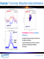
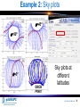
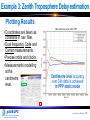
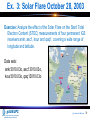
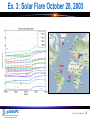
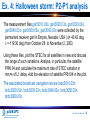
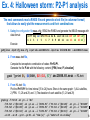
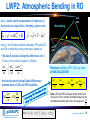
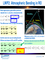
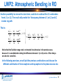
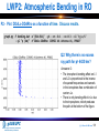
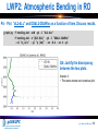
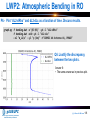
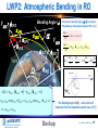
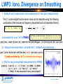
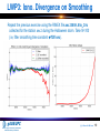
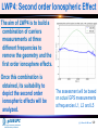
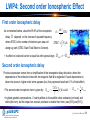
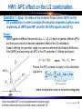
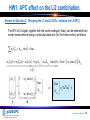
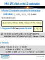
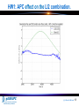
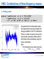
1
Tutorial 5 Analysis of propagation effects from GNSS observables based on laboratory exercises Contact: [email protected] Web site: http://www.gage.upc.edu Slides associated to gLAB version 2.0.0 gAGE/UPC Research group of Astronomy & Geomatics Technical University of Catalonia @ J. Sanz & J.M. Juan 1 Authorship statement The authorship of this material and the Intellectual Property Rights are owned by J. Sanz Subirana and J.M. Juan Zornoza. These slides can be obtained either from the server http://www.gage.upc.edu, or [email protected]. Any partial reproduction should be previously authorized by the authors, clearly referring to the slides used. This authorship statement must be kept intact and unchanged at all times. gAGE/UPC Research group of Astronomy & Geomatics Technical University of Catalonia @ J. Sanz & J.M. Juan 2 OVERVIEW Introduction The gLAB tool suite Examples of GNSS Data Processing using gLAB Laboratory session organization LABORATORY Session Starting up your laptop Basic: Introductory lab exercises: Iono & Posit, SF, storm,TIDs Medium: Laboratory Work Projects: LWP1 to LWP4 Advanced: Homework gAGE/UPC Research group of Astronomy & Geomatics Technical University of Catalonia @ J. Sanz & J.M. Juan 3 Introduction This tutorial is devoted to analysing and assessing different issues associated with GNSS signal propagation effects in the atmosphere. The laboratory exercises will be developed with actual GPS measurements, and processed with the ESA/UPC GNSS-Lab Tool suite (gLAB), which is an interactive software package for GNSS data processing and analysis. All software tools (including gLAB) and associated files for the laboratory session are included in the USB stick delivered to those who attend the lecture. The laboratory session will consist of a set of exercises organized in three different levels of difficulty (Basic, Medium and Advanced). A set of introductory examples range from a first glance assessment of the ionosphere effects on single frequency positioning, and Zenith Tropospheric Delays estimate to showing different perturbation effects in the ionosphere (Solar Flair, Halloween storm, TIDs). Electron density profiles (Ne) retrieval, bending effects analysis (phase excess rate depicture), as well as in-depth analysis of the code-carrier ionosphere divergence on single-frequency smoothed codes and the second order ionospheric effects are analysed in detail in four Laboratory Work Projects. Other topics are given as homework. The target is to provide the participants with a wide range of selected exercises to choose from, according their interests and their level of knowledge of these topics. gAGE/UPC Research group of Astronomy & Geomatics Technical University of Catalonia @ J. Sanz & J.M. Juan 4 OVERVIEW Introduction The gLAB tool suite Examples of GNSS Data Processing using gLAB Laboratory session organization LABORATORY Session Starting up your laptop Basic: Introductory lab exercises: Iono & Posit, SF, storm,TIDs Medium: Laboratory Work Projects: LWP1 to LWP4 Advanced: Homework gAGE/UPC Research group of Astronomy & Geomatics Technical University of Catalonia @ J. Sanz & J.M. Juan 5 The gLAB Tool suite The GNSS-Lab Tool suite (gLAB) is an interactive multipurpose educational and professional package for GNSS Data Processing and Analysis. gLAB has been developed under the ESA Education Office contract N. P1081434. Main features: • High Accuracy Positioning capability. • Fully configurable. • Easy to use. • Access to internal computations. gAGE/UPC Research group of Astronomy & Geomatics Technical University of Catalonia @ J. Sanz & J.M. Juan 6 The gLAB Tool suite Students/Newcomers: • Easy to use: Intuitive GUI. • Explanations: Tooltips over the different GUI options. • Guidelines: Several error and warning messages. Templates for pre-configured processing. Professionals/Experts: • Powerful tool with High Accuracy Positioning capability. • Fast to configure and use: Templates and carefully chosen defaults. • Can be executed in command-line and included in batch processing. gAGE/UPC Research group of Astronomy & Geomatics Technical University of Catalonia @ J. Sanz & J.M. Juan 7 The gLAB Tool suite In order to widen the tool availability, gLAB Software has been designed to work in both Windows and Linux environments. The package contains: • Windows binaries (with an installable file). • Linux .tgz file. • Source code (to compile it in both Linux and Windows OS) under an Apache 2.0 license. • Example data files. • Software User Manual. • HTML files describing the standard formats. gAGE/UPC Research group of Astronomy & Geomatics Technical University of Catalonia @ J. Sanz & J.M. Juan 8 The gLAB Tool suite Read files capability: • RINEX observation v2.11 & v3.00 • RINEX navigation message. • SP3 precise satellite clocks and orbits files • ANTEX Antenna information files. • Constellation status. • DCBs files. • GPS_Receiver_Type files. • SINEX position files. Modelling module: Pre-processing module: • Carrier-phase pre-alignment. • Carrier-phase / pseudo-range consistency check. • Cycle-slip detection (customizable parameters) - Melbourne-Wübbena. - Geometry-free CP combination. - L1-C1 difference (single frequency). • Pseudo-range smoothing. • Decimation capability. • On demand satellite enable/disable. • Elevation mask. • Frequency selection. • Discard eclipsed satellites. gAGE/UPC Research group of Astronomy & Geomatics Technical University of Catalonia Backup • • • • • • • • • • • Fully configurable model. Satellite positions. Satellite clock error correction. Satellite movement during signal flight time. Earth rotation during signal flight time. Satellite phase center correction. Receiver phase center correction. (frequency dependent). Relativistic clock correction. Relativistic path range correction. Ionospheric correction (Klobuchar). Tropospheric correction - • • • Simple and Niell mappings. Simple and UNB-3 nominals. Differential Code Bias corrections. Wind up correction. Solid tides correction (up to 2nd degree). @ J. Sanz & J.M. Juan 9 The gLAB Tool suite Filtering module: • • • • • • • Able to chose different measurements to process (1 or more), with different weights. This design could be useful in future Galileo processing, where processing with different measurements may be desired. Fixed or elevation-dependent weights per observation. Troposphere estimation on/off. Carrier-Phase or Pseudo-range positioning. Static/Kinematic positioning (full Q/Phi/P0 customization). Able to do a forward/backward processing. Able to compute trajectories (no need for a priori position). gAGE/UPC Research group of Astronomy & Geomatics Technical University of Catalonia Output module: • Cartesian / NEU coordinates. • Configurable message output. Other functionalities: Backup • • • Computation of satellite coordinates and clocks from RINEX and SP3 files. Satellite coordinates comparison mode. For instance RINEX navigation vs. SP3, or SP3 vs. SP3 (along-track, cross-track and radial orbit errors, clock errors, SISRE). Show input mode. No processing, only parsing RINEX observation files. • Current version allows full GPS data processing, and partial handling of Galileo and GLONASS data. • Future updates may include full GNSS data processing. @ J. Sanz & J.M. Juan 10 GNSS learning material package Includes three different parts, allowing participants to follow either a guided or a self-learning GNSS course: • GNSS Book: Complete book with theory, practical examples, and with a Laboratory course on GNSS Data Processing & Analysis [R-1]. • gLAB tool suite: Source code and binary software files, plus configuration files, allowing processing GNSS data from standard formats. The options are fully configurable through a GUI. GPS Data Processing: Code and Phase Algorithms, Techniques and Recipes Image courtesy of USAF Research Laboratory gAGE-NAV Research group of Astronomy & Geomatics Satellite Navigation, LLC http://www.gage.es Manuel Hernández Pajares José Miguel Juan Zornoza Jaume Sanz Subirana • gAGE-GLUE: Bootable USB stick with a full environment ready to use; based on LINUX (Ubuntu) OS. gAGE/UPC Research group of Astronomy & Geomatics Technical University of Catalonia @ J. Sanz & J.M. Juan 11 OVERVIEW Introduction The gLAB tool suite Examples of GNSS processing using gLAB Laboratory session organization LABORATORY Session Starting up your laptop Basic: Introductory lab exercises: Iono & Posit, SF, storm,TIDs Medium: Laboratory Work Projects: LWP1 to LWP4 Advanced: Homework gAGE/UPC Research group of Astronomy & Geomatics Technical University of Catalonia @ J. Sanz & J.M. Juan 12 Examples of GNSS Data Processing using gLAB Example 1: Ionospheric effects on single frequency positioning. • This exercise is devoted to analysing the effect of the ionospheric error in single frequency positioning. This is done both in the Signal-In-Space (SIS) and User Domains. • A receiver will be positioned in Standard Point Positioning (SPP) mode: a) with full modelling, b) neglecting the ionospheric correction. gAGE/UPC Research group of Astronomy & Geomatics Technical University of Catalonia @ J. Sanz & J.M. Juan 13 Example 1: Iono effects on single freq. Posit. Data set: 24h data collected by the IGS permanent receiver “ramo” (Lon,Lat ) on May 4th 2000. May 4, 2000 gAGE/UPC Research group of Astronomy & Geomatics Technical University of Catalonia @ J. Sanz & J.M. Juan 14 Example 1: Iono effects on single freq. Posit. 1. Compute SPP using files: ramo1250.00o,brdc1250.00n 2 1 4 3 5 gLAB.out Equivalent command line sentence: gLAB_linux -input:cfg gLAB_p1_Full.cfg -input:obs ramo1250.00o gAGE/UPC brdc1250.00n Research group of Astronomy &-input:nav Geomatics Technical University of Catalonia @ J. Sanz & J.M. Juan 15 Example 1. NEU Position Error plot from gLAB.out FULL SPP model NEU plot template configuration gLAB.out Equivalent command line sentence: North East gAGE/UPC Research group of Astronomy & Geomatics Technical University of Catalonia Up graph.py -f gLAB.out -x4 -y18 -s.- -c '($1=="OUTPUT")' -l "North error" -f gLAB.out -x4 -y19 -s.- -c '($1=="OUTPUT")' -l "East error" -f gLAB.out -x4 -y20 -s.- -c '($1=="OUTPUT")' -l "UP error“ --yn -20 --yx 50 --xl "time (s)" --yl "error (m)" -t "NEU positioning error [SPP]: Full model" @ J. Sanz & J.M. Juan 16 Example 1. gLAB Modeling panel The different model terms can be analyzed with gLAB: The modeling options set in this panel are applied by default to the SPP solution. gAGE/UPC Research group of Astronomy & Geomatics Technical University of Catalonia •Using the previous data file, the impact of neglecting the ionospheric correction is evaluated in the Range and Position domains. •This is a baseline example of this analysis procedure. The same scheme must be applied for all model terms (troposphere, relativistic correction...). A full analysis of the different model components can be found in [R-2].) @ J. Sanz & J.M. Juan 17 Example 1. Model component analysis: IONO. The procedure explained here is applicable for all model terms: iono, tropo… Default 1.In Modeling panel, configuration disable the model for SPP component to analyze. 1 Disable Ionospheric correction (in this example: disable Ionospheric correction) 2.Save as gLAB1.out the associated output file. In the Default configuration the output file was gLAB.out gAGE/UPC Research group of Astronomy & Geomatics Technical University of Catalonia Notice that the gLAB.out file contains the processing results with the FULL model, as was set in the default configuration. 2 Set output file Equivalent command line sentence: as gLAB1.out 3 18 @ J. Sanz & J.M. Juan gLAB_linux -input:cfg gLAB_p1_NoIono.cfg -input:obs ramo1250.00o -input:nav brdc1250.00n Example 1. NEU Position Error plot from gLAB1.out No Iono. correction NEU plot template configuration gLAB1.out Equivalent command line sentence: North East gAGE/UPC Research group of Astronomy & Geomatics Technical University of Catalonia Up graph.py -f gLAB1.out -x4 -y18 -s.- -c '($1=="OUTPUT")' -l "North error" -f gLAB1.out -x4 -y19 -s.- -c '($1=="OUTPUT")' -l "East error" -f gLAB1.out -x4 -y20 -s.- -c '($1=="OUTPUT")' -l "UP error“ --yn -20 --yx 50 --xl "time (s)" --yl "error (m)" -t "NEU positioning error [SPP]: No Iono. Corr." @ J. Sanz & J.M. Juan 19 Example 1. VPE plot from gLAB.out,gLAB1.out 1 Click Clear to restart plots Y-min, Y-max 2 3 gLAB1.out gLAB.out gAGE/UPC Research group of Astronomy & Geomatics Technical University of Catalonia Time (sec) Vertical @ J. Sanz & J.M. Juan 20 Example 1. HPE plot: gLAB.out, gLAB1.out 1 Click Clear to restart plots X-min, Y-min, Y-max 2 gLAB1.out gAGE/UPC Research group of Astronomy & Geomatics Technical University of Catalonia 3 gLAB.out East: 19 North: 18 @ J. Sanz & J.M. Juan 21 Example 1. Klobuchar iono. corr. plot: gLAB.out Code delay Carrier advance Ionosphere delays code and advances carrier measurements. gLAB.out gAGE/UPC Research group of Astronomy & Geomatics Technical University of Catalonia Select IONO Note: Use the gLAB.out file. In gLAB1.out file this model component was switched off. @ J. Sanz & J.M. Juan 22 Example 1. Measur. (P2-P1) v.s. Model (Klobuchar) P2-P1=STEC+Krec+Ksat gLAB.out gAGE/UPC Research group of Astronomy & Geomatics Technical University of Catalonia Y-min=0 Y-max=40 @ J. Sanz & J.M. Juan 23 Example 1. Summary: Klobuchar model performance gLAB1.out gLAB1.out gLAB.out gLAB.out gLAB.out Code delay gAGE/UPC Research group of Astronomy & Geomatics Technical University of Catalonia Ionospheric correction (broadcast Klobuchar ) Ionospheric delays are larger at noon due to the higher illumination. Large positioning errors (mainly in vertical) appear when neglecting ionospheric corrections. @ J. Sanz & J.M. Juan 24 Example 1. 2-frequency Ionosphere-free solution From previous configuration set following options gLAB2.out 1 Disable Iono correct. and (P1-P2) TGDs 2-frequencies Iono-free (PC) 2 3 After running gLAB, plot results as in previous cases gAGE/UPC Research group of Astronomy & Geomatics Technical University of Catalonia Equivalent command line sentence: gLAB_linux -input:cfg gLAB_pc_IFree.cfg@ J. Sanz & J.M. Juan 25 -input:obs ramo1250.00o -input:nav brdc1250.00n Example 1. Single-frequency vs. Dual-frequency 1-freq.[SPS]: with Klobuchar gLAB.out gLAB.out 2-freq.: Iono-free Plot gLAB2.out results as in previous cases ramo station location gLAB2.out gAGE/UPC Research group of Astronomy & Geomatics Technical University of Catalonia gLAB2.out May 4, 2000 @ J. Sanz & J.M. Juan 26 Example 1: Iono effects on single freq. Posit. Ionospheric delay The ionosphere extends from about 60 km over the Earth’s surface until more than 2000 km, with a sharp electron density maximum at around 350 km. The ionospheric refraction depends, among other things, on the location, local time and solar cycle (11 years). • First order (~99.9%) ionospheric delay on the inverse of squared frequency: I1 depends where STEC is the number of electrons per area unit along ray path (STEC: Slant Total Electron Content). I1 = 40.3 STEC f2 STEC = ∫ N e ds • Two-frequency receivers can remove this error source f12 P1 − f 22 P 2 (up to 99.9%) using ionosphere-free combination PC = of pseudo-ranges (PC) or carriers (LC). f12 − f 22 • Single-frequency users can remove about a 50-70% of the ionospheric delay using the Klobuchar model, whose parameters are broadcast in the GPS navigation message. gAGE/UPC Research group of Astronomy & Geomatics Technical University of Catalonia Backup @ J. Sanz & J.M. Juan 27 Example 1: Iono effects on single freq. Posit. Annex: gLAB processing in command line gAGE/UPC Research group of Astronomy & Geomatics Technical University of Catalonia @ J. Sanz & J.M. Juan 28 Example 1: gLAB processing in command line Execute in a single line: (gnuplot can also be used ) graph.py -f gLAB.out -x4 -y18 -f gLAB.out -x4 -y19 -f gLAB.out -x4 -y20 --yn -20 -t "NEU -s.- -c '($1=="OUTPUT")' -l "North error" -s.- -c '($1=="OUTPUT")' -l "East error" -s.- -c '($1=="OUTPUT")' -l "UP error" --yx 50 --xl "time (s)" --yl "error (m)" positioning error [SPP]: Full model" graph.py -f gLAB.out -x4 -y20 -s.- -c '($1=="OUTPUT")' --l "Full model" -f gLAB1.out -x4 -y20 -s.- -c '($1=="OUTPUT")' --l "No Iono." --cl r --yn -20 --yx 50 --xl "Time (s)" --yl "Up error (m)" -t "Vertical positioning error [SPP]" graph.py -f gLAB1.out -x19 -y18 -so -c '($1=="OUTPUT")' --l "No Iono." --cl r -f gLAB.out -x19 -y18 -so -c '($1=="OUTPUT")' --l "Full mod" --cl b --xl "East error (m)" --yl "North error (m)" --xn -20 --xx 20 --yn -20 --yx 20 -t "Horizontal pos. error [SPP]" graph.py -f gLAB.out -x4 -y25 -s. -c '($1=="MODEL")' -f gLAB.out -x4 -y'($10-$9)' -s. -c '($1=="INPUT")‘ --cl r --xl "time (s)" --yl "meters" --yn -0 --yx 40 -t "Ionospheric Combination" gAGE/UPC Research group of Astronomy & Geomatics Technical University of Catalonia @ J. Sanz & J.M. Juan 29 29 Example 1: gLAB processing in command line Console to execute “command line” sentences gAGE/UPC Research group of Astronomy & Geomatics Technical University of Catalonia A “notepad” with the command line sentence is provided to facilitate the sentence writing: just “copy” and “ paste” from notepad to the working terminal. @ J. Sanz & J.M. Juan 30 Example 1: gLAB processing in command line The different messages provided by gLAB and its content can be found in the [OUTPUT] section. By placing the mouse on a given message name, a tooltip appears describing the different fields. In console mode: execute gLAB_linux -messages gAGE/UPC Research group of Astronomy & Geomatics Technical University of Catalonia Backup @ J. Sanz & J.M. Juan 31 Example 2: Ionospheric delay analysis Example 2: Depict the ionospheric delays for the different satellites in view from station amc2 • This is a simple exercise aimed to illustrate how to use gLAB to easily analyze GNSS measurements and their combinations. • gLAB will used to read the RINEX measurements file and to generate a “text” with the measurements provided in a columnar format (more suitable to make plots). • From “text” file, compute PI ≡ P2 − P1 =I + K 21 and plot the Ionospheric LI ≡ L1 − L2 =I + Ambiguity delay for a given satellite, P1 − L1= 2α1 I + ambiguity1 by using code and carrier measurements at f1, f2: P2 − L2= 2α 2 I + ambiguity 2 gAGE/UPC Research group of Astronomy & Geomatics Technical University of Catalonia @ J. Sanz & J.M. Juan 32 Ionospheric combination (meters) Example 2: Ionospheric delay analysis Code P2-P1 (unambiguous but noisier) The target is to generate this plot to depict the ionospheric delay from code & carrier data PI ≡ P2 − P1 =I + K 21 LI ≡ L1 − L2 =I + Ambiguity Ambiguity= P − L Carrier Phase L1-L2 (ambiguous but precise) P1 − L1= 2α1 I + ambiguity1 P2 − L2= 2α 2 I + ambiguity 2 α1 = = γ 21 gAGE/UPC Research group of Astronomy & Geomatics Technical University of Catalonia 1 = 1.546 ; α 2 = 1 + α1 γ 21 − 1 f1 / f 2 ) (= 2 (154 / 120) 2 @ J. Sanz & J.M. Juan 33 Example2: GPS measurements content Code measurement content Carrier measurement content P2 =+ ρ α 2 ( I + K 21 ) + ε 2 L1 = ρ − α1 I + B1 + ς 1 L2 =ρ − α 2 I + B2 + ς 2 P1 =+ ρ α1 ( I + K 21 ) + ε1 ρ α1 = 1 = 1.546 γ 21 − 1 γ 21 = ( f1 / f 2 ) 2 Refers to all non dispersive terms: geometric range, clocks, tropo. delay… (see [R-1]). Ionospheric delay I 1 α 2 − α1 = 40.3 ( f − f 2 1 2 2 2 2 1 2 f f ) 10 16 STEC = ∫ sat rec N e dl , ( STEC is in TECUs ) STEC ; ( I is in m of L1 − L2 delay) = 16 − 1 TECU 10 = e / m 2 0.10m of L1- L 2 delay Interfrequency bias = K 21 K 21,rec − K 21sat As the satellite clocks are referred to the ionosphere-free combination of codes (PC), the K 21sat cancels in such combination. f12 P1 − f 22 P2 P = Note: TGD = −α1 K 21sat is broadcast in GPS nav. Message. C f12 − f 22 Carrier ambiguities = Bi λi N i + bi gAGE/UPC Research group of Astronomy & Geomatics Technical University of Catalonia Ni is an integer number. bi is a real number (fractional part of ambiguity) Backup @ J. Sanz & J.M. Juan 34 Example 2: Ionospheric delay analysis 1.- Read RINEX file with gLAB and generate a “measurements file” in a columnar format (the easiest to manipulate and plot content): Using the configuration file meas.cfg, READ the RINEX and generate the MEAS file: gLAB_linux -input:cfg meas.cfg -input:obs coco0090.97o -input:nav brdc0090.97n > coco.meas gLAB configuration file -pre:dec 1 -print:none -print:meas --model:satphasecenter --model:recphasecenter --model:satclocks --pre:cs:li --pre:cs:bw gAGE/UPC Research group of Astronomy & Geomatics Technical University of Catalonia RINEX Measurement file RINEX Navigation file OUTPUT: measurement file in columnar format [Id YY Doy sec GPS PRN el Az N. list C1C L1C C1P L1P C2P L2P] 1 2 3 4 5 6 7 8 9 10 11 xx xx 14 15 16 ] @ J. Sanz & J.M. Juan 35 Example 2: Ionospheric delay analysis 2.- Manipulate the file with the easy & powerful awk (or gawk) programming language (to compute the combinations of measurements): From coco.meas file: P1 L1 P2 L2 ] [Id YY Doy sec GPS PRN el Az N. list C1C L1C C1P L1P C2P L2P] 1 2 3 4 5 6 7 8 9 10 11 xx xx 14 15 16 Compute different ionospheric combination of codes and carriers, and generate the obs.txt file containing the fields: [PRN,sec, P2-P1, (P2-L2)/5.09, (P1-L1)/3.09, L1-L2, Elev/10] gawk '{print $6,$4,$15-$11,($15-$16)/5.09,($11-$14)/3.09,$14-$16,$7/10}' coco.meas > obs.txt PRN #6 (P2-P1) (L1-L2) #15 -- #11 #14 -- #16 sec #4 gAGE/UPC Research group of Astronomy & Geomatics Technical University of Catalonia (P2-L2)/5.09 (P1-L1)/3.09 #15 -- #16 #11-- #14 Elev/10 #7 @ J. Sanz & J.M. Juan 36 Example 2: Ionospheric delay analysis 3.-Plot results with “graph.py” (you can use the gnuplot as well) From obs.txt file: [PRN, sec, P2-P1, (P2-L2)/5.09, (P1-L1)/3.09, L1-L2, Elev/10] 1 2 3 4 5 6 7 Show in the same plot the following iono. delays for satellite PRN01: P2-P1, (P2-L2)/5.09, (P1-L1)/3.09, L1-L2, Elev./10 Condition: Select PRN01 (from 1-st field) File to plot Fields to plot: #2 (x-axis) versus #3 (y-axis) graph.py -f obs.txt -c'($1==01)' -x2 -f obs.txt -c'($1==01)' -x2 -f obs.txt -c'($1==01)' -x2 -f obs.txt -c'($1==01)' -x2 -f obs.txt -c'($1==01)' -x2 --yn -10 --yx 15 --xl "time gAGE/UPC Research group of Astronomy & Geomatics Technical University of Catalonia Label: P2-P1 -y3 --l "P2-P1" –y4 --l "(P2-L2)/5.09" -y5 --l "(P1-L1)/3.09" –y6 --l "L1-L2" –y7 --l "Elev/10" (s)" --yl "meters of L1-L2 delay" @ J. Sanz & J.M. Juan 37 Example 2: Ionospheric delay analysis PI ≡ P2 − P1 =I + K 21 LI ≡ L1 − L2 =I + Ambiguity P1 − L1= 2α1 I + ambiguity1 zoom P2 − L2= 2α 2 I + ambiguity 2 α1 = = γ 21 gAGE/UPC Research group of Astronomy & Geomatics Technical University of Catalonia 1 = 1.546 ; α 2 = 1 + α1 γ 21 − 1 f1 / f 2 ) (= 2 (154 / 120) 2 @ J. Sanz & J.M. Juan 38 Example 2: Sky plots Φ=40º Φ=90º Φ=0º coco Sky plots at different latitudes PRN01 gAGE/UPC Research group of Astronomy & Geomatics Technical University of Catalonia @ J. Sanz & J.M. Juan 39 Example 3: Zenith Troposphere Delay estimation PPP Template: Static positioning with dual freq. code & carrier (ionospherefree combination PC,LC) + post-processed precise orbits & clocks. 1. Select the PPP Template 2. Upload data files: -Measurement : roap1810.09o - ANTEX: igs05_1525.atx - Orbits & clocks: igs15382.sp3 - SINEX: igs09P1538.snx 2 1 gAGE/UPC Research group of Astronomy & Geomatics Technical University of Catalonia 3. RUN gLAB 3 Default output file: gLAB.out @ J. Sanz & J.M. Juan 40 Example 3: Zenith Troposphere Delay estimation Plotting Results • Coordinates are taken as constants in nav. filter. • Dual frequency Code and Carrier measurements. • Precise orbits and clocks. • Measurements modelling at the centimetre level. gAGE/UPC Research group of Astronomy & Geomatics Technical University of Catalonia Centimetre level accuracy over 24h data is achieved in PPP static mode @ J. Sanz & J.M. Juan 41 Example 3: Zenith Troposphere Delay estimation The troposphere is estimated as a Random Walk process in the Kalman Filter. A process noise of 1cm/sqrt(h) has been taken. 1 2 ftp://cddis.gsfc.nasa.gov/pub/gps/products/troposphere/new/2009/181/roap1810.09zpd.gz The ZTD in this file is given in mm of delay. Thus, it is converted to m to compare with gLAB results grep ROAP roap1810.09zpd | gawk -F\: '{print $3} ' | gawk '{print $1,$2/1000}' > roap_igs.trp gAGE/UPC Research group of Astronomy & Geomatics Technical University of Catalonia @ J. Sanz & J.M. Juan 42 Example 3: Zenith Troposphere Delay estimation Tropospheric delay The troposphere is the atmospheric layer situated between the Earth’s surface and an altitude of about 50 km. The effect of the troposphere on GNSS signals appears as an extra delay in the measurement of the signal travelling from satellite to receiver. The tropospheric delay does not depend on frequency and affects both the pseudo-range (code) and carrier phases in the same way. It can be modeled by: • A hydrostatic component, composed of dry gases (mainly nitrogen and oxygen) in hydrostatic equilibrium. This component can be treated as an ideal gas. Its effects vary with the temperature and atmospheric pressure in a reasonably predictable manner, and it is responsible for about 90% of the delay. • A wet component caused by the water vapor condensed in the form of clouds. It depends on the weather conditions and varies faster than the hydrostatic component and in a totally random way. For high accuracy positioning, this component must be estimated together with the coordinates and other parameters in the navigation filter. gAGE/UPC Research group of Astronomy & Geomatics Technical University of Catalonia Backup @ J. Sanz & J.M. Juan 43 OVERVIEW Introduction The gLAB tool suite Examples of GNSS processing using gLAB Laboratory session organization LABORATORY Session Starting up your laptop Basic: Introductory lab exercises: Iono & Posit, SF, storm,TIDs Medium: Laboratory Work Projects: LWP1 to LWP4 Advanced: Homework gAGE/UPC Research group of Astronomy & Geomatics Technical University of Catalonia @ J. Sanz & J.M. Juan 44 Laboratory session organization The laboratory session is organized as an assisted activity where a set of exercises must be developed individually or in groups of two. As they are conceived as self-learning work, a detailed guide is provided in the slides (pdf file) to carry out the exercises. A notepad file with the command line instructions is also provided to help the sentence writing (doing copy & paste). A set of questions is presented, and the answers are also included in the slides. Teachers will attend individual (or collective) questions that could arise during exercise resolution. gAGE/UPC Research group of Astronomy & Geomatics Technical University of Catalonia @ J. Sanz & J.M. Juan 45 Laboratory session organization The exercises are organized at three different levels of difficulty. The student can choose the level of exercises to do, although at least one introductory exercise is recommended to learn basic gLAB usage. 1. Basic: Introductory exercises. From 1 to 6. They consist of simple exercises to: 1) Study the Ionosphere effects on single frequency positioning. 2) To depict the STEC on a Radio occulation 3) Solar Flare effect on TEC, 4,5) TEC evolution during the Halloween Storm, 6) To depict a TID propagaction. a gAGE/UPC Research group of Astronomy & Geomatics Technical University of Catalonia GP @ J. Sanz & J.M. Juan 46 Laboratory session organization 2. Medium: Laboratory Work Projects (LWP). Four different LWP are proposed (to choose from): • LWP1: To show a simple numerical method to estimate electron density profiles (Ne(h)) from RO data. • LWP2: To analyse the phase excess rate from GPS to LEO due to atmospheric (ionosphere & troposphere) bending. a G P Ne a Courtesy of UCAR Actual measurements from FORMOSAT-3/COSMIC LEOs will be used ρ∼ GP ρ A minimum knowledge of UNIX (e.g., awk) would be desirable gAGE/UPC Research group of Astronomy & Geomatics Technical University of Catalonia LWP1 LWP2 @ J. Sanz & J.M. Juan 47 Laboratory session organization 2. Medium: Laboratory Work Projects (LWP). Four different LWP are proposed (to choose from): • LWP3: To study the code-carrier ionosphere divergence effect on single-frequency carrier smoother code. Bi f i f • LWP4: To analyse if second-order ionospheric effects can be depicted from three-frequency GNSS measurements. Given that session time is limited to 3h, students who feel comfortable using gLAB, can skip part of the previous basic exercises (Ex1, Ex2,.. ) and jump to the Lab. Work Project. A minimum knowledge of UNIX (e.g., awk) would be desirable gAGE/UPC Research group of Astronomy & Geomatics Technical University of Catalonia @ J. Sanz & J.M. Juan 48 Laboratory session organization 3 . Advanced: Labeled as “Homework exercises” A set of additional exercises addressed to those students that already have a solid background in GPS data processing. These exercises are beyond the scope of this 3h laboratory session, and are given for a possible further discussion… As in the previous cases, the answers to the questions are also included as BACKUP slides. A minimum knowledge of UNIX (e.g., awk) is desirable for these homework exercises. ∑α k k Lk + ∑ α k ∆ kUP sin ε = bias k APC correction term 7427cB0 cos θ 7257c sat − θ − I 2 L1 = N B ds STEC cos e 3 ∫rec 3 2 f1 2 f1 gawk 'BEGIN{g=(77/60)^2}{print $6, $4, (g*($13-$14)-($15-$16))/(g-1)}' meas.txt > PC.txt gAGE/UPC Research group of Astronomy & Geomatics Technical University of Catalonia @ J. Sanz & J.M. Juan 49 OVERVIEW Introduction The gLAB tool suite Examples of GNSS processing using gLAB Laboratory session organization LABORATORY Session Starting up your laptop Basic: Introductory lab exercises: Iono & Posit, SF, storm,TIDs Medium: Laboratory Work Projects: LWP1 to LWP4 Advanced: Homework gAGE/UPC Research group of Astronomy & Geomatics Technical University of Catalonia @ J. Sanz & J.M. Juan 50 Starting up your laptop 1. Plug the stick into an USB port and boot your laptop from the stick. 2. Access the Boot Device Menu when starting up the laptop. Note: The way to do it depends on your computer: Usually, you should press [ESC] or [F4], [F10], [F12].... gAGE/UPC Research group of Astronomy & Geomatics Technical University of Catalonia @ J. Sanz & J.M. Juan 51 Starting up your laptop 3. The following screen will appear after about 2 minutes: Click on this icon to open a console The US keyboard is set by default. You can change it by clicking on the upper right corner. Click on the gLAB icon to start-up gLAB gAGE/UPC Research group of Astronomy & Geomatics Technical University of Catalonia @ J. Sanz & J.M. Juan 52 Starting up your laptop Now, the system is ready to start working! Console to execute “command line” sentences gAGE/UPC Research group of Astronomy & Geomatics Technical University of Catalonia @ J. Sanz & J.M. Juan 53 Starting up your laptop Console to execute “command line” sentences gAGE/UPC Research group of Astronomy & Geomatics Technical University of Catalonia Copy and paste the sentences from notepad to console @ J. Sanz & J.M. Juan 54 OVERVIEW Introduction The gLAB tool suite Examples of GNSS processing using gLAB Laboratory session organization LABORATORY Session Starting up your laptop Basic: Introductory lab exercises: Iono & Posit, Solar Flair, Halloween storm,TIDs Medium: Laboratory Work Projects: LWP1 to LWP4 Advanced: Homework gAGE/UPC Research group of Astronomy & Geomatics Technical University of Catalonia @ J. Sanz & J.M. Juan 55 EX. 1 Halloween storm: October 2003 A severe ionospheric storm was experienced on October 29-31, 2003 producing and increase of the electron density which led to large ionospheric refraction values on the GPS signals. Such conditions were beyond the capability of the GPS Klobuchar model broadcast for single frequency users, producing large errors in the SPS (see details in [R-3]). Dual frequency users, navigating with the ionospheric-free combination of GPS signals were not affected by such ionospheric errors, as the ionospheric refraction can be removed up to 99:9% using dualfrequency signals. gAGE/UPC Research group of Astronomy & Geomatics Technical University of Catalonia Backup @ J. Sanz & J.M. Juan 56 Ex. 1: Assessing Iono effects on single freq. pos. Exercise: Repeat the previous study of Example 1 to analyze the single freq. solution, but for the Halloween storm. The following steps are recommended: 1. Using files amc23020.03o,brdc3030.03n compute with gLAB the following solutions: 1. Solution with full SPS modeling. Name output file as: gLAB.out 2. Solution with the ionospheric corrections disabled gLAB1.out 3. Solution with the 2-freq. Ionosphere-free code (PC) gLAB2.out 2. Plot results Note: The gLAB GUI or the command line sentences can also be used . A “notepad” with the command line sentence is provided to facilitate the sentence writing: just “copy” and “paste” from notepad to the working terminal gAGE/UPC Research group of Astronomy & Geomatics Technical University of Catalonia @ J. Sanz & J.M. Juan 57 Ex. 1: Full processing gLAB.out 1. Compute SPP using files: amc23020.03o,brdc3030.03n 2 By default, the output file name is gLAB.out 1 3 Equivalent command line sentence: gLAB_linux -input:cfg gLAB_p1_Full.cfg -input:obs amc3030.03o gAGE/UPC brdc3030.03n Research group of Astronomy &-input:nav Geomatics Technical University of Catalonia @ J. Sanz & J.M. Juan 58 Ex. 1: Iono. Disabled gLAB1.out 2. Reprocess the same files, with the iono. corrections disabled 2 Disable Ionospheric corrections 1 Change output file name to gLAB1.out 3 Equivalent command line sentence: gLAB_linux -input:cfg gLAB_p1_NoIono.cfg -input:obs amc3030.03o gAGE/UPC brdc3030.03n Research group of Astronomy &-input:nav Geomatics Technical University of Catalonia @ J. Sanz & J.M. Juan 59 Ex. 1: Processing with PC gLAB2.out 3. Reprocess the same files, but with 2-frequency ionosphere-free (PC) 1 Disable Ionospheric corrections and P1P2 corrections Equivalent command line sentence: gLAB_linux -input:cfg gLAB_p1_IFree.cfg -input:obs amc3030.03o gAGE/UPC brdc3030.03n Research group of Astronomy &-input:nav Geomatics Technical University of Catalonia 2 Select Dual Frequency 3 Change output file name to gLAB2.out 4 @ J. Sanz & J.M. Juan 60 60 Ex. 1: Assessing Iono effects on single freq. pos. Execute in a single line: (or use the gLAB GUI) graph.py -f gLAB.out -x4 -y18 -s.- -c '($1=="OUTPUT")' -f gLAB.out -x4 -y19 -s.- -c '($1=="OUTPUT")' -f gLAB.out -x4 -y20 -s.- -c '($1=="OUTPUT")' --yn -40 --yx 70 --xl "time (s)" -t "NEU positioning error [SPP]: -l "North error" -l "East error" -l "UP error" --yl "error (m)" Full model" graph.py -f gLAB.out -x4 -y20 -s.- -c '($1=="OUTPUT")' --l "Full model" -f gLAB1.out -x4 -y20 -s.- -c '($1=="OUTPUT")' --l "No Iono." --cl r --yn -40 --yx 90 --xl "Time (s)" --yl "Up error (m)" -t "Vertical positioning error [SPP]" graph.py -f gLAB1.out -x19 -y18 -so -c '($1=="OUTPUT")' --l "No Iono." --cl r -f gLAB.out -x19 -y18 -so -c '($1=="OUTPUT")' --l "Full mod" --cl b --xl "East error (m)" --yl "North error (m)" --xn -40 --xx 40 --yn -40 --yx 40 -t "Horizontal pos. error [SPP]" P2-P1 shifted +4 m graph.py -f gLAB.out -x4 -y'($10-$9+4)' -s. -c '($1=="INPUT")' -f gLAB.out -x4 -y25 -s. -c '($1=="MODEL")' --cl r --xl "time (s)" --yl "meters" --yn -5 --yx 80 -t "Ionospheric Combination" gAGE/UPC Research group of Astronomy & Geomatics Technical University of Catalonia @ J. Sanz & J.M. Juan 61 61 Ex. 1: Assessing Iono effects on single freq. pos. gLAB1.out gLAB.out gLAB.out gLAB1.out gLAB.out Ionospheric correction (broadcast Klobuchar ) Ionospheric delays are larger at noon due to the higher insulation. Code delay gAGE/UPC Research group of Astronomy & Geomatics Technical University of Catalonia Klobuchar model is unable to mitigate the large ionospheric errors during the storm. Position domain errors reach up to 40 meters with Klobuchar corrections used. @ J. Sanz & J.M. Juan 62 Ex. 1: Assessing Iono effects on single freq. pos. 1-freq.[SPS]: with Klobuchar Ionospheric correction (broadcast Klobuchar ) •The ionosphere-free combination (PC) of P1 and P2 codes is immune to the ionospheric storm. • Although PC is three-times noisier than P1 or P2, it provides positioning accurate at the level of a few meters during the storm. f 2P − f 2P PC = 2-freq.: Iono-free 1 1 2 1 2 2 2 2 f −f amc2 station location October 30, 2003 gAGE/UPC Research group of Astronomy & Geomatics Technical University of Catalonia @ J. Sanz & J.M. Juan 63 Ex. 2: STEC in a Radio Occultation (RO) Radio Occultation (RO) commonly refers to a sounding technique in which a radio signal from a transmitting satellite (e.g., GPS) passes through a planetary atmosphere before arriving at a receiver on board a Low Earth Orbiter (LEO) satellite. Along the ray path, the phase of the radio signal is perturbed in a manner related to the refractivity. RO measurements can reveal the refractivity, from which one can then derive atmospheric quantities such as Pressure, Temperature and the partial pressure of water vapor; and electron density, among others. gAGE/UPC Research group of Astronomy & Geomatics Technical University of Catalonia a GP This is a simple exercise where the STEC variation along a radio occultation will be depicted using GPS L1, L2 measurements from a receiver on board a LEO of COSMIC constellation. In the LWP1, Electron Density Profiles will be retrieved from this data using an algorithm equivalent to the Abel Transform. @ J. Sanz & J.M. Juan 64 FORMOSAT-3/COSMIC mission Constellation Observing System for Meteorology Ionosphere and Climate: 6 microsatellites; orbit altitude ~ 800km • Three instruments: GPS receiver. 4 antennas: 2 for POD, 2 for RO. TIP, Tri-band beacon • Weather + Space Weather data. • Global observations of: Pressure, Temperature, Humidity Refractivity Ionospheric Electron Density Ionospheric Scintillation • Demonstrate quasi-operational GPS limb sounding with global coverage in near-real time • Climate Monitoring Courtesy of UCAR Courtesy of UCAR Information available at www.cosmic.ucar.edu gAGE/UPC Research group of Astronomy & Geomatics Technical University of Catalonia @ J. Sanz & J.M. Juan 65 Ex. 2: STEC in a Radio Occultation (RO) Exercise: The file “RO.obs” contains the following fields [*]: YY DoY HH.HH CODE PRN 1 2 3 4 5 |------ LEO ------>|<------- GPS ------->| elev r_LEO AR_LEO DEC_LEO r_GPS AR_GPS DEC_GPS L1 L2 (deg) (km) (Deg) (Deg) (km) (Deg) (Deg) (cycles) 6 7 8 9 10 11 12 13 14 L1-L2 arc (m) 15 16 Plot the L1-L2 measurement in function of time to depict the variation of STEC along the occultation: Select for instance : PRN=02 and “CODE=l241”, that corresponds to LEO=4 and Antenna 1 - Selecting: CODE=l241 and PRN=02 grep l241 RO.obs|gawk '{if ($5==02) print $3,$15}'> ro.dat - Ploting L1-L2 graph.py -f ro.dat --xl "time (H)" --yl "meters of L1-L2" -t"RO: L1-L2: COSMIC #4 Antenna #1" [*] This file has been generated from files (http://cosmic-io.cosmic.ucar.edu/cdaac): podObs_2006.253.004.01.01_rnx, leoOrb_2006.253.004.01_2009.2650_sp3, igs13920.sp3 gAGE/UPC Research group of Astronomy & Geomatics Technical University of Catalonia @ J. Sanz & J.M. Juan 66 66 Ex. 2: STEC in a Radio Occultation (RO) The previous plot shows only the variation of the Integrated Electron Content along the ray path (STEC). More information can be retrieved from occultation measurements. For instance: • Electron Density Profile of the Ionosphere (LWP1). • Phase excess rate, which is related to the bending of ray (LWP2). a G P Ne a ∼ ρ G P ρ gAGE/UPC Research group of Astronomy & Geomatics Technical University of Catalonia @ J. Sanz & J.M. Juan 67 Given that session time is limited to 2h, participants who feel comfortable using gLAB, can skip part of the next basic exercises (Ex3..., Ex6) and jump to the Laboratory Work Projects (LWP). There, if you prefer, you can jump to slide #87 and choose one from the four LWPs gAGE/UPC Research group of Astronomy & Geomatics Technical University of Catalonia @ J. Sanz & J.M. Juan 68 Ex. 3: Solar Flare October 28, 2003 On October 28, 2003, an intense solar eruption (a Solar Flare) was detected around 11h UT in an active region which had grown one of the largest sunspots ever seen by the SOlar Helioscopic Observatory (SOHO). It appeared as a bright spike in the SOHO ultraviolet images. This sudden enhancement of the solar radiation in the X-ray and extreme ultra-violet band produced a sudden increase in the ionospheric electron density on the daylight hemisphere, (see [R-3]). gAGE/UPC Research group of Astronomy & Geomatics Technical University of Catalonia @ J. Sanz & J.M. Juan 69 Ex. 3: Solar Flare October 28, 2003 Exercise: Analyze the effect of the Solar Flare on the Slant Total Electron Content (STEC) measurements of four permanent IGS receivers ankr, asc1, kour and qaq1, covering a wide range of longitude and latitude. qaq1 Data sets: ankr3010.03o, asc13010.03o, kour3010.03o, qaq13010.03o ankr kour asc1 gAGE/UPC Research group of Astronomy & Geomatics Technical University of Catalonia @ J. Sanz & J.M. Juan 70 Ex. 3: Solar Flare October 28, 2003 Execute: gLAB_linux gLAB_linux gLAB_linux gLAB_linux -input:cfg -input:cfg -input:cfg -input:cfg [Id YY Doy sec GPS PRN el Az N. list C1C L1C C1P L1P C2P L2P] 1 2 3 4 5 6 7 8 9 10 11 xx 13 14 15 16 ] meas.cfg meas.cfg meas.cfg meas.cfg -input:obs -input:obs -input:obs -input:obs ankr3010.03o asc13010.03o kour3010.03o qaq13010.03o graph.py -f ankr3010.03.meas -x4 -y'($14-$16)' --l -f asc13010.03.meas -x4 -y'($14-$16)' --l -f kour3010.03.meas -x4 -y'($14-$16)' --l -f qaq13010.03.meas -x4 -y'($14-$16)' --l --xl "time (s)" --yl "meters of L1-L2" --xn 38500 --xx 40500 --yn -20 --yx 20 -t "28 Oct 2003 Solar flare" gAGE/UPC Research group of Astronomy & Geomatics Technical University of Catalonia > > > > ankr3010.03.meas asc13010.03.meas kour3010.03.meas qaq13010.03.meas "ankr" "asc1" "kour" "qaq1" qaq1 ankr kour asc1 @ J. Sanz & J.M. Juan 71 Ex. 3: Solar Flare October 28, 2003 qaq1 ankr kour asc1 gAGE/UPC Research group of Astronomy & Geomatics Technical University of Catalonia @ J. Sanz & J.M. Juan 72 Ex. 4: Halloween storm: P2-P1 analysis Associated with the Solar Flare analysed in the previous exercise, a Coronal Mass Ejection occurred, which sent a large particle cloud impacting the Earth's magnetosphere about 19 hours later, on October 29. Subsequent impacts were still occurring several hours later. This material interacted with the Earth's magnetosphere and a Storm Enhancement Density (SED) appeared in North America and affected later the northern latitudes in Europe. Extra large gradients of TEC associated with this phenomenon were also produced, degrading the GPS positioning performance. The TEC evolution in October 30, 2003 (i.e., Day 303 of year 2003) can be seen in the movie TEC 2003oct30 anim.gif. gAGE/UPC Research group of Astronomy & Geomatics Technical University of Catalonia @ J. Sanz & J.M. Juan 73 Ex. 4: Halloween storm: P2-P1 analysis The measurement files garl3010.03o, garl3020.03o, garl3030.03o, garl3040.03o, garl3050.03o, garl3060.03o were collected by the permanent receiver garl in Empire, Nevada, USA ( φ= 40.42 deg, λ =-119:36 deg) from October 28 to November 2, 2003. Using these files, plot the STEC for all satellites in view and discuss the range of such variations. Analyse, in particular, the satellite PRN 04 and calculate the maximum rate of STEC variation in mm=s of L1 delay. Add the elevation of satellite PRN 04 in the plot. The associated broadcast navigation les are brdc3010.03n, brdc3020.03n, brdc3030.03n, brdc3040.03n, brdc3050.03n, brdc3060.03n. gAGE/UPC Research group of Astronomy & Geomatics Technical University of Catalonia @ J. Sanz & J.M. Juan 74 Ex. 4: Halloween storm: P2-P1 analysis Exercise: Depict the ionospheric delays for the different satellites in view from station amc2 • This is a simple exercise aimed to illustrate how to use gLAB to easily analyze GNSS measurements and their combinations. • gLAB will used to read the RINEX measurements file and to generate a “text” with the measurements provided in a columnar format (more suitable to make plots). • Using such “text” file, the STEC pattern for the different satellites in view during the storm is depicted from the geometry-free combination of codes P2-P1. Note: P2 − P1 =I + K 21 gAGE/UPC Research group of Astronomy & Geomatics Technical University of Catalonia @ J. Sanz & J.M. Juan 75 Ex. 4: Halloween storm: P2-P1 analysis The next commands read a RINEX file and generate a text file (in columnar format) that allows to easily plot the measurements and their combinations: 1. Using the configuration file meas.cfg, READ the RINEX and generate the MEAS message with data format: [Id YY Doy sec GPS PRN el Az N. list C1C L1C C1P L1P C2P L2P] 1 2 3 4 5 6 7 8 9 10 11 xx 13 14 15 16 ] Execute: gLAB_linux -input:cfg meas.cfg -input:obs amc23030.03o -input:nav brdc3030.03n > amc23030.03.meas 2. From meas.txt file, Compute the ionospheric combination of codes: PI=P2-P1. Generate the file PI.txt with the following content: [PRN, hour, PI, elevation] gawk '{print $6, $4/3600, $15-$13, $7}' amc23030.03.meas > PI.txt 3. From PI.txt file, Plot the PI=P2-P1 for time interval [15 to 24].hours. Show in the same graph: 1) ALL satellites, 2) PRN 13, 28 and 29, and 3) The elevation of each satellite.(13, 28 and 29) graph.py -f PI.txt -x2 -y3 --l "ALL" -f PI.txt -c'($1==28)' -x2 -y3 -so --l "28:P2-P1" -f PI.txt -f PI.txt -c'($1==29)' -x2 -y3 -so --l "29:P2-P1" -f PI.txt -f PI.txt -c'($1==13)' -x2 -y3 -so --l "13:P2-P1" -f PI.txt gAGE/UPC --xn --xx& Geomatics 25 --yn 0 --yx 85 --xl "time (s)" --yl "meters Research group15 of Astronomy Technical University of Catalonia Backup -c'($1==28)' -x2 -y4 --l "29:ELEV" -c'($1==29)' -x2 -y4 --l "13:ELEV" -c'($1==13)' -x2 -y4 --l "13:ELEV" 76 of L1-L2 delay" @ J. Sanz & J.M. Juan 76 Ex. 4: Halloween storm: P2-P1 analysis amc2 station location October 30, 2003 gAGE/UPC Research group of Astronomy & Geomatics Technical University of Catalonia @ J. Sanz & J.M. Juan 77 Ex. 5: Halloween storm evolution Exercise: Analyze the ionospheric delays for 6 consecutive days including the Halloween storm • This is a simple exercise aimed to illustrate the ionospheric delays variation during the Halloween storm. A period of 6 consecutive days (from October 28 to November 2, 2003) are analyzed using measurements collected in the “garl” station in North America. • The STEC variations are depicted from the geometry-free combination of codes P2-P1. Note: P2 − P1 =I + K 21 gAGE/UPC Research group of Astronomy & Geomatics Technical University of Catalonia @ J. Sanz & J.M. Juan 78 Ex. 5: Halloween storm evolution 1.- Read RINEX file: gLAB_linux gLAB_linux gLAB_linux gLAB_linux gLAB_linux gLAB_linux -input:cfg -input:cfg -input:cfg -input:cfg -input:cfg -input:cfg meas.cfg meas.cfg meas.cfg meas.cfg meas.cfg meas.cfg [Id YY Doy sec GPS PRN el Az N. list C1C L1C C1P L1P C2P L2P] 1 2 3 4 5 6 7 8 9 10 11 xx 13 14 15 16 ] -input:obs -input:obs -input:obs -input:obs -input:obs -input:obs garl3010.03o garl3020.03o garl3030.03o garl3040.03o garl3050.03o garl3060.03o -input:nav -input:nav -input:nav -input:nav -input:nav -input:nav brdc3010.03n brdc3020.03n brdc3030.03n brdc3040.03n brdc3050.03n brdc3060.03n > > > > > > garl3010.03.meas garl3020.03.meas garl3030.03.meas garl3040.03.meas garl3050.03.meas garl3060.03.meas 2.- Merge files and refer all the data to 0h of October 28th: Doy0301: cat garl30?0.03.meas |gawk '{d=($3-301)*86400;$4=$4+d; print $6, $4/3600, $15-$13, $7}' > PI.txt 3.- Plot results: graph.py -f PI.txt –x2 –y3 --l "ALL P2-P1" -f PI.txt -c'($1==04)' –x2 –y4 --l "PRN04: ELEV" -f PI.txt -c'($1==04)' –x2 –y3 –so --l "PRN04: P2-P1" --xn 0 --xx 144 gAGE/UPC Research group of Astronomy & Geomatics Technical University of Catalonia @ J. Sanz & J.M. Juan 79 Ex. 5: Halloween storm evolution Zoom at time interval: 70 to 78 h graph.py -f PI.txt –x2 –y3 --l "ALL P2-P1" -f PI.txt -c'($1==04)' –x2 –y4 --l “04: EL" -f PI.txt -c'($1==04)' –x2 –y3 –so --l “04" --xn 0 --xx 144 gAGE/UPC Research group of Astronomy & Geomatics Technical University of Catalonia graph.py -f PI.txt –x2 –y3 --l "ALL P2-P1" -f PI.txt -c'($1==04)' –x2 –y4 --l “04: EL" -f PI.txt -c'($1==04)' –x2 –y3 –so --l “04" --xn 70 --xx 78 @ J. Sanz & J.M. Juan 80 Ex. 6: Travelling Ionospheric Disturb. Travelling Ionospheric Disturbances (TIDs) are understood as plasma density fluctuations that propagate through the ionosphere at an open range of velocities and frequencies. The trend of such fluctuations can be seen from L1 − L2 . the geometry free combination of GPS carrier measurements L= I Some authors distinguish between Large-Scale TIDs (LSTIDs) with a period greater than 1 hour and moving faster than 0,3 km/s, and Medium- Scale TIDs (MSTIDs) with shorter periods (from 10 minutes to 1 hour) and moving slower (0.05-0.3 km/s). The LSTIDs seem to be related to geomagnetic disturbances (i.e., aurora, ionospheric storms, etc.). The origin of MSTIDs seems to be more related to meteorological phenomena such as neutral winds, eclipses, or solar terminator that produces Atmospheric Gravity Waves (AGW) being manifested as TIDs at ionospheric heights, due to the collision between neutral and ionised molecules. gAGE/UPC Research group of Astronomy & Geomatics Technical University of Catalonia @ J. Sanz & J.M. Juan 81 Ex. 6: Travelling Ionospheric Disturb. In [R4, 2006] a simple method to detect MSTIDs is proposed. It consists of detrending the geometry free combination of GPS carrier measurements from the diurnal variation and elevation angle dependences, applying the following equation: δ LI (t= ) LI (t ) − ( LI (t + τ ) − LI (t − τ ) ) / 2 where a value of 300sec is suitable to keep enough variation of LI (i.e., STEC). Using the previous equation, the detrending is done simply by subtracting from each value an average value of the previous and posterior measurements (i.e., the curvature of the LI temporal dependency). It must be pointed out that that this detrending procedure can be used in real time with a single receiver, so it is suitable for identifying these ionospheric perturbations in navigation applications. gAGE/UPC Research group of Astronomy & Geomatics Technical University of Catalonia @ J. Sanz & J.M. Juan 82 Ex. 6: Travelling Ionospheric Disturb. An example of MSTID propagation can be depicted as follows using the measurements of three stations SODB, MHCB and MONB, which are separated by a few tens of kilometres. monb The target is to reproduce the figure 10 of the above mentioned paper [R4, 2006]. mhcb sodb [R4, 2006] Hernández-Pajares, M; Juan, M.; Sanz, J., 2006]. gAGE/UPC Research group of Astronomy & Geomatics Technical University of Catalonia @ J. Sanz & J.M. Juan 83 Ex. 6: Travelling Ionospheric Disturb. Exercise: Execute in a single line: # a) Reading RINEX files: gLAB_linux -input:cfg meas.cfg -input:obs mhcb2910.01o > mhcb.meas gLAB_linux -input:cfg meas.cfg -input:obs monb2910.01o > monb.meas gLAB_linux -input:cfg meas.cfg -input:obs sodb2910.01o > sodb.meas # b) gawk gawk gawk Selecting satellite '{if ($6==14) print '{if ($6==14) print '{if ($6==14) print PRN16: $0}' mhcb.meas > mhcb_14.meas $0}' monb.meas > monb_14.meas $0}' sodb.meas > sodb_14.meas monb mhcb sodb # c) Detrending on the geometry-free combination L1-L2: gawk '{for (i=0;i<21;i++) {t[i]=t[i+1];l[i]=l[i+1]};t[21]=$4;l[21]=$14-$16; if (NR>21){tt=t[0]*t[10]*t[20];if (tt!=0) print t[10],(l[10]-(l[0]+l[20])/2)}}' mhcb_14.meas > mhcb_dLi.meas gawk '{for (i=0;i<21;i++) {t[i]=t[i+1];l[i]=l[i+1]};t[21]=$4;l[21]=$14-$16; if (NR>21){tt=t[0]*t[10]*t[20];if (tt!=0) print t[10],(l[10]-(l[0]+l[20])/2)}}' monb_14.meas > monb_dLi.meas gawk '{for (i=0;i<21;i++) {t[i]=t[i+1];l[i]=l[i+1]};t[21]=$4;l[21]=$14-$16;if (NR>21){tt=t[0]*t[10]*t[20]; if (tt!=0) print t[10],(l[10]-(l[0]+l[20])/2)}}' sodb_14.meas > sodb_dLi.meas gAGE/UPC Research group of Astronomy & Geomatics Technical University of Catalonia @ J. Sanz & J.M. Juan 84 Ex. 6: Travelling Ionospheric Disturb. Execute in a single line: graph.py -f sodb_dLi.meas -s.- --l "sodb: PRN14" -f mhcb_dLi.meas -s.- --l "mhcb: PRN14" -f monb_dLi.meas -s.- --l "monb: PRN14" --xn 55500 --xx 57000 --yn -0.05 --yx 0.07 --xl "time (s)" --yl "Detrended STEC (meters of L1-L2 delay)" -t "MS Travelling Ionospheric Disturbance (MSTID) propagation" monb mhcb gAGE/UPC Research group of Astronomy & Geomatics Technical University of Catalonia sodb @ J. Sanz & J.M. Juan 85 OVERVIEW Introduction The gLAB tool suite Examples of GNSS processing using gLAB Laboratory session organization LABORATORY Session Starting up your laptop Basic: Introductory lab exercises: Iono & Posit, SF, storm,TIDs Medium: Laboratory Work Projects: LWP1 to LWP4 Advanced: Homework gAGE/UPC Research group of Astronomy & Geomatics Technical University of Catalonia @ J. Sanz & J.M. Juan 86 LWP1: Electron Density Profile from RO In the previous Exercise #2 the variation of the Integrated Electron Content along the ray path (STEC) has been shown. From these integrated measurements during an occultation it is possible to retrieve the electron density profile (i.e., Ne(h)) of the ionosphere. gAGE/UPC Research group of Astronomy & Geomatics Technical University of Catalonia a G P Ne LWP1: Target In this LWP we will retrieve the Ne(h) using a simple numerical algorithm which is equivalent to the Abel transform (see [R-6]). @ J. Sanz & J.M. Juan 87 LWP1: Electron Density Profile from RO • The basic observable of this technique is the additional delay, due to the refractivity index, of a radio signal when passing through the atmosphere. • This additional delay is proportional to the integrated refractivity, in such a way that we can obtain an estimation of the vertical refractivity profiles using observations at different elevation angles by solving an inverse problem. • Traditionally, the solution of this inverse problem is obtained by using the Abel inversion algorithm assuming a refractivity index that only depends on the altitude (see [RD-6]) gAGE/UPC Research group of Astronomy & Geomatics Technical University of Catalonia a Ne GP As it is know, STEC and Ne are related by: STEC ( p ) = ∫ LEO GPS N e dl An equivalent expression, assuming spherical symmetry STEC ( pn ) 2∑ i =1 N e ( pi ) li ,n n where p stands for the impact parameter (the closest point to the Earth centre along the optical ray path). @ J. Sanz & J.M. Juan 88 LWP1: Electron Density Profile from RO Thence, starting from the outer ray (p1=rLEO), for a given ray i, where i=1,…, with impact parameter pi, its STEC can be written in a discrete representation as: STEC ( pi ) 2 N e ( pi ) li ,i + = j = i −1 ∑ N (p ) l j =1 e j i, j where lii is the fraction of ith ray within the spherical layer ith (see [R-6]). The previous equation defines a triangular linear equations system that can be solved recursively for the electron density Ne(p). gAGE/UPC Research group of Astronomy & Geomatics Technical University of Catalonia L1 −= L2 α STEC + b where p stands for the impact parameter (the closest point to the Earth centre along the optical ray path). As measurements we use L1-L2 carrier phases that are related with the STEC by: L1 −= L2 α STEC + b where the bias term b is eliminated making differences to a reference in the arch data. @ J. Sanz & J.M. Juan 89 89 LWP1: Electron Density Profile from RO The program “abel.perl” implements the previous algorithm to estimate the Ne(p) profile from GPS L1-L2 carrier measurements. • The input data is [p(n),L1-L2(n)], with p in km and L1-L2 in meters (of L1-L2 delay) where the impact parameter must be sorted from larger to lower value. Only measurements with negative elevation must be given (i.e., occultation). • The output data is: [n,p(n),L1-L2(n),Ne(n)], where Ne is given in e-/m3. Note: the Impact parameters can be computed from the LEO elevation (elev) and its distance to Earth’s centre (rLEO) by (see figure): p = rLEO cos(elev) gAGE/UPC Research group of Astronomy & Geomatics Technical University of Catalonia @ J. Sanz & J.M. Juan 90 LWP1: Electron Density Profile from RO Exercise: The file “RO.obs” contains the following fields (see Ex.5): YY DoY HH.HH CODE PRN 1 2 3 4 5 |------ LEO ------>|<------- GPS ------->| elev r_LEO AR_LEO DEC_LEO r_GPS AR_GPS DEC_GPS L1 L2 (deg) (km) (Deg) (Deg) (km) (Deg) (Deg) (cycles) 6 7 8 9 10 11 12 13 14 L1-L2 arc (m) 15 16 1.- Using the file RO.obs, select the measurements with negative elevations for GPS satellite PRN02, the LEO #4 and antenna #1, and generate the input file [p(n),L1-L2(n)] for program “abel.perl” - Selecting: CODE=l241 and PRN=02 and negative elevations (ocult) grep l241 RO.obs|gawk '{if ($5==02 && $6<0) print $0}'> ro.tmp - Generating the input file gawk '{printf "%9.5f %7.5f \n",$7*cos($6*3.14/180),$15}' ro.tmp > abl.tmp - Sort the file by impact parameter: sort –nr –k+1 abl.tmp > abl.dat gAGE/UPC Research group of Astronomy & Geomatics Technical University of Catalonia @ J. Sanz & J.M. Juan 91 LWP1: Electron Density Profile from RO 2.- Run the program “abel.perl” over the generated file “abl.dat“ to compute the electron density profile Ne(p): - Sort the file by impact parameter: cat abl.dat| abel.perl > Ne.dat 3.- The output file “abl.dat“ contains the fields [n,p(n),L1-L2(n),Ne(n)] Plot the electron density profile Ne as a function the impact parameter p and as a function of height above Earth‘s - Plot1: As a function of “p” graph.py -f Ne.dat -x4 -y2 --xl "Ne(e-/m3)" --yl "p (km)" - Plot2: As a function of “height” graph.py -f Ne.dat -x4 –y’($2-6370)’ --xl "Ne(e-/m3)" --yl “h (km)" gAGE/UPC Research group of Astronomy & Geomatics Technical University of Catalonia @ J. Sanz & J.M. Juan 92 LWP1: Electron Density Profile from RO Questions 1. Taking into account the relationship between the electron density (Ne) and the critical frequency (fp), i.e., minimum frequency for a signal not being reflected, [R-1]: f p = 8.98 N e ( N e in e − /m3 , f p in Hz) Compute the minimum frequency of a signal to cross through the ionosphere. Answer: From previous plot, the Ne of the maximum is 3.7E+11 e-/m3. Thence 11 = f p 8.98 3.7 ⋅10 = 5.46 MHz 2. Calculate the height where a signal with frequency f=4 MHz will be reflected, according to the previous plot of Ne profile. Answer: gAGE/UPC Research group of Astronomy & Geomatics Technical University of Catalonia N e =( f / 8.98) 2 =(4 ⋅106 / 8.98) 2 = 1.98 ⋅1011 ⇒ 150 km @ J. Sanz & J.M. Juan 93 LWP2: Atmospheric Bending in RO LWP2: Target This LWP is focused in depicting and analysing the effect of the atmospheric bending in Radio Occultation measurements. a ρ∼ G P ρ A simple procedure will be given to depict the phase excess rate due to the troposphere and ionosphere over L1, L2 and LC measurements. Note: LC is the Ionosphere Free combination of carriers L1 and L2 is given by: gAGE/UPC Research group of Astronomy & Geomatics Technical University of Catalonia LC = f12 L1 − f 22 L 2 f12 − f 22 @ J. Sanz & J.M. Juan 94 LWP2: Atmospheric Bending in RO a Let L1 be the carrier measurement at frequency f1. A procedure to depict the L1 bending is given next: sat L1 = ρ * + cdtrec + B1 ; ρ * = ρ + T − α1 I being ρ the Euclidean distance between GPS and LEO and B a constant bias along continuous phase arc G P Ref. GPS No bending a ρ∼ G P Bending ρ Ref. LEO • The bias B cancels, taking time differences of L1. Thence, from previous equation, it follows sat ∆ρ * ∆L1 ∆cdtrec = − ∆t ∆ t ∆ t • And clocks cancel taking Double-Differences between pairs of LEO and GPS satellites: ∆L j ∆ρ * DD = DD ∆t ∆t gAGE/UPC Research group of Astronomy & Geomatics Technical University of Catalonia Reference satellites (GPS, LEO) are taken in NON-OCULTATION . * ∆ρ occult ∆t − ∆ρ occult = ∆t DD ∆L j ∆t − DD ∆ρ ≠0 ∆t Note: LEO and GPS orbits are known at the level of few cm (~5cm), thus the Euclidean range can be calculated accurately and, thus, the range rate ∆ρ ∆t GPSRef GPSRef GPS DD() =()GPS LEO − () LEO − () LEORef − () LEORef @ J. Sanz & J.M. Juan 95 LWP2: Atmospheric Bending in RO Next expressions generalize previous results for L1, L2 and Lc measurements: sat + B j ; ρ * = ρ + T − α j I ; j = 1, 2 L j = ρ * + cdtrec sat ρ + cdtrec + BC ; ρ = ρ +T LC = a And the clock term cancels taking Double Differences between LEO and GPS satellites * ∆ρ occult ∆t ∆ρ occult ∆t ∆ρ occult ∆L ∆ρ = DD j − DD ≠ 0 ; j= 1, 2 ∆t ∆t ∆t * ∆ρ occult ∆L ∆ρ − = DD C − DD ≠ 0 Carrier Excess Rate ∆t ∆t ∆t − gAGE/UPC Research group of Astronomy & Geomatics Technical University of Catalonia Ref. GPS No bending a ρ∼ G P Bending ρ The differences in time to depict the bending sat ∆L ∆ρ * ∆L j ∆cdtrec ∆ρ * =− ⇒ DD = DD j ∆t ∆t ∆t ∆t ∆t sat ∆L ∆ρ ∆LC ∆cdtrec ∆ρ = − ⇒ DD = DD C ∆t ∆t ∆t ∆t ∆t G P Ref. LEO Reference satellites (GPS, LEO) are taken in NON-OCULTATION . Bending is assumed only for the GPS-LEO ray in occultation. GPSRef GPSRef GPS DD() =()GPS − ( ) − ( ) − ( ) LEO LEO LEORef LEORef @ J. Sanz & J.M. Juan 96 LWP2: Atmospheric Bending in RO Another possibility to remove the clock term, could be to subtract the LC combination from L1 (or L2). The result will provide the “discrepancy between L1 (or L2) and LC excess ray path. That is: * ∆ρ occult sat ∆L j ∆cdtrec =− ; j= 1, 2 * ∆ρ occult ∆ρ occult ∆L j ∆LC ∆t ∆t ∆t − = − ; j= 1, 2 ⇒ sat ∆t ∆t ∆t ∆t ∆ρ occult ∆LC ∆cdtrec = − ∆t ∆t ∆t Notice that the Euclidian range rate is not needed to subtract as in the previous case, because it is cancelled when taking the difference between L1 (or L2) and Lc. Other delays can also be cancelled... In the following exercises, we will plot the previous combinations and discuss the different contribution of the ionosphere and troposphere to the phase excess rate. gAGE/UPC Research group of Astronomy & Geomatics Technical University of Catalonia @ J. Sanz & J.M. Juan 97 LWP2: Atmospheric Bending in RO Exercise: The program “RO.perl” uses the “RO.obs” as input data and computes the following combinations of RO measurements: The output file: 1 2 3 sec CODE PRN 4 p 5 6 7 8 9 10 11 12 13 14 dRho dL1 dL2 dLc d(L1-Lc) d(L2-Lc) DDdRho DDdL1 DDdL2 DDLc (units m/s) where • Rho is the Euclidean Distance between GPS and LEO • d: means differences in time • DD: means Double Differences between GPS and LEOs satellites. Note: the GPS PRN13 and LEO “l252” are used as reference satellites. (the rays between these satellites are not in occultation). a G P Ref. GPS No bending The results are computed for the RO between GPS PRN02 and LEO “l241” (the same occultation as in previous cases) The aim of this exercise is to analyse the phase excess rate in the different combinations due to the bending of the ray. gAGE/UPC Research group of Astronomy & Geomatics Technical University of Catalonia a G P Bending Ref. LEO @ J. Sanz & J.M. Juan 98 LWP2: Atmospheric Bending in RO 1.- Run the program “RO.perl” over the file “RO.obs” and generate the combinations of measurements indicated in the previous table. Note: the results are provided for the occultation associate to PRN=02 and “CODE=l241”, that corresponds to LEO=4 and Antenna 1. This is hard code in the program, but can be changed, as well. - Execute (the file RO.obs, must be available in the directory) RO.perl > bending.dat 2.- Discuss next plots: gAGE/UPC Research group of Astronomy & Geomatics Technical University of Catalonia @ J. Sanz & J.M. Juan 99 LWP2: Atmospheric Bending in RO P1.- Plot “DDdL1-DDdRho” and DDdL2-DDdRho as a function of time and discuss the results found graph.py -f bending.dat -x'($12-$11)' -y4 -f bending.dat -x'($13-$11)' -y4 -l "DDdL1-DDdRho" -l "DDdL2-DDdRho" --xn -0.4 --xx 4 Q1: Justify the discrepancy between the two plots. Answer 1: • The curves in the plot show phase excess rate due the effect of both ionosphere and troposphere. • As the bending in the ionosphere is a frequency dependent effect, the contribution is different for each signal (L1 and L2). gAGE/UPC Research group of Astronomy & Geomatics Technical University of Catalonia @ J. Sanz & J.M. Juan 100 LWP2: Atmospheric Bending in RO P2.- Plot DDdLc-DDdRho as a function of time. Discuss results. graph.py -f bending.dat -x'($14-$11)' -y4 --xn -0.1 --xx 0.3 --xl "m_Lc/s" --yl "p (km)" -t"DDdLc-DDdRho: COSMIC #4 Antenna #1, PRN02" Q2: Why there is no excess ray path for p> 6420 km? Answerer 2: • The ionospheric bending effect on L1 and L2 is proportional to the inverse of squared frequencies and cancels in the ionosphere-free combination of carriers Lc. • There is only bending effect in Lc due to the troposphere, which produces the path at the bottom of the figure. gAGE/UPC Research group of Astronomy & Geomatics Technical University of Catalonia @ J. Sanz & J.M. Juan 101 LWP2: Atmospheric Bending in RO P3.- Plot “dL1-dLc” and DDdL1-DDdRho as a function of time. Discuss results. graph.py -f bending.dat –x9 -y4 -l "dL1-dLc" -f bending.dat -x'($12-$11)' –y4 -l "DDdL1-DDdRho" --xl "m_L1/s" --yl "p (km)" --xn -0.4 --xx 4 -y4 Q3: Justify the discrepancy between the two plots. Answer 3: • DDdL1-DDdRho accounts for the contribution of ionosphere and troposphere. The troposphere produces the large drift at the bottom. • dL1-dLc cancels common effects in both signals, like troposphere and ionosphere. But, as there is no bending effect due to the ionosphere on Lc (see previous plot P2) , thence, the curves match for p> 6420 km. gAGE/UPC Research group of Astronomy & Geomatics Technical University of Catalonia @ J. Sanz & J.M. Juan 102 LWP2: Atmospheric Bending in RO P4.- Plot “dL2-dLc” and DDdL2-DDdRho as a function of time. Discuss results. graph.py -f bending.dat –x10 -y4 -l "dL2-dLc" -f bending.dat -x'($13-$11)' –y4 -l "DDdL1-DDdRho" --xl "m_L2/s" --yl "p (km)" --xn -0.4 --xx 4 -y4 Q4: Justify the discrepancy between the two plots. Answer 4: • The same answer as in previous plot. gAGE/UPC Research group of Astronomy & Geomatics Technical University of Catalonia @ J. Sanz & J.M. Juan 103 LWP2: Atmospheric Bending in RO P5.- Plot “dL1-dRho” and dL1-dLc as a function of time. Discuss results. graph.py -f bending.dat -x'($6-$5)' -y4 -l "dL1-dRho" -f bending.dat –x9 -y4 -l "dL1-dLc" --xl "m_L1/s" --yl "p (km)" -t"COSMIC #4 Antenna #1, PRN02" Q5: Justify the discrepancy between the two plots. Answer 5: • The large drift in dL1-dRho curve is due to the satellites (GPS and LEO) clock drift. • These large clock variations do not allow to see the atmospheric bending effect. gAGE/UPC Research group of Astronomy & Geomatics Technical University of Catalonia @ J. Sanz & J.M. Juan 104 LWP2: Atmospheric Bending in RO P6.- Plot “dL2-dRho” and dL2-dLc as a function of time. Discuss results. graph.py -f bending.dat -x'($7-$5)' -y4 -l "dL2-dRho" -f bending.dat –x10 -y4 -l "dL2-dLc" --xl "m_L2/s" --yl "p (km)" -t"COSMIC #4 Antenna #1, PRN02" Q6: Justify the discrepancy between the two plots. Answer 6: • The same answer as in previous plot. gAGE/UPC Research group of Astronomy & Geomatics Technical University of Catalonia @ J. Sanz & J.M. Juan 105 LWP2: Atmospheric Bending in RO VGPS φGPS τ a GP κGPSτ GPS κvGPS αGPS θGPS Bending Angle (α) κLEO α αLEO rGPS Ω Derivation of bending angle α(a) from Excess Phase Rate (or Atmospheric Doppler Shift λ ∆f ) ∆ρ occult VvLEO LEO φκLEO θLEO LEO τ ∆t * ∆ρ occult ∆t ∆f λ= = ( v GPS − v LEO ) ⋅ τ = v GPS ⋅ k GPS − v LEO ⋅ k LEO * ∆ρ occult ∆t − ∆ρ occult = ∆t DD ∆L j ∆t − DD ∆ρ ∆t rLEO λ ∆= f v GPS ⋅ ( k GPS − τ ) − v LEO ⋅ ( k LEO − τ ) = + θ LEO ) a nGPS rGPS sin(α = nLEO rLEO sin(α LEO GPS + θ GPS ) α α GPS + α LEO gAGE/UPC Research group of Astronomy & Geomatics Technical University of Catalonia The Bending Angle α ( a ) can be derived iteratively from this equations system (see, [R-7]) Backup @ J. Sanz & J.M. Juan 106 LWP2: Atmospheric Bending in RO Comments: From phase excess rate measurements the bending angle can be estimated. From the bending angle, the variations of the refractivity can be computed, and from these one can then derive atmospheric quantities such as Pressure, Temperature and the partial pressure of water vapor, and electron density, among others. gAGE/UPC Research group of Astronomy & Geomatics Technical University of Catalonia Backup @ J. Sanz & J.M. Juan 107 LWP3: Iono. Divergence on Smoothing The target of LWP3 is to analyze the error induced by the divergence of the ionosphere (between code and carrier) into the SingleFrequency (SF) carrier smoothed code. The Divergence Free (Dfree) and the Ionosphere Free (IFree) smoothed codes will be compared with the SF one. gAGE/UPC Research group of Astronomy & Geomatics Technical University of Catalonia This effect will be analyzed analytically and tested with single and double frequency GPS measurements under large ionospheric gradients. @ J. Sanz & J.M. Juan 108 LWP3: Iono. Divergence on Smoothing The noisy code can be smoothed with the precise (but ambiguous) carrier measurements. This carrier smoothing can be done in real-time applying the Hatch filter. The smoothing depends on the time smoothing constant or filter length. The more the filter length is used, the more smoothed the code is, but (with single frequency measurements) a higher code-carrier divergence error is induced by the ionosphere. This is because the ionospheric refraction has opposite sign on code and carrier, being its effect twice on the difference of code and carrier. This double ionospheric refraction is propagated forward through the filter, producing a bias. The error induced by the code-carrier divergence of the ionosphere on the single frequency smoothed codes is assessed in this exercise for different filter lengths. gAGE/UPC Research group of Astronomy & Geomatics Technical University of Catalonia @ J. Sanz & J.M. Juan 109 LWP3: Iono. Divergence on Smoothing n −1 1 Pˆ= P(k ) + (k ) ( P(k − 1) + L(k ) − L(k − 1) ) n n k if k < N ], and [n = N if k ≥ N ]. where [n = The algorithm is initialised with: Pˆ (1) = P(1). The previous algorithm can be interpreted as real-time alignment of carrier with code: 1 n −1 Pˆ= P(k ) + (k ) 1) ) ( P(k − 1) + L(k ) − L(k −= n n = L(k ) + P − L ( k ) where P − L ( k= ) gAGE/UPC Research group of Astronomy & Geomatics Technical University of Catalonia n −1 1 P−L ( P (k ) − L(k ) ) + n n ( k −1) Ionospheric combination (meters) The noisy code P can be smoothed with the precise (but ambiguous) carrier L measurements. This carrier smoothing can be done in real-time applying the Hatch filter. Code P (unambiguous but noisier) Ambiguity= P − L Carrier Phase L (ambiguous but precise) 1 ∑ ( P (k ) − L(k ) ) n @ J. Sanz & J.M. Juan 110 LWP3: Iono. Divergence on Smoothing Time varying ionosphere induces a bias in the single frequency smoothed code when it is averaged in the smoothing filter. This effect is analysed as follows: Where ρ includes all non dispersive terms (geometric range, clock offsets, troposphere) and I1 represents the frequency dependent terms (ionosphere and DCBs). B1 Is the carrier ambiguity, which is constant along continuous carrier phase arcs and ε1 , ς 1 account for code and carrier multipath and thermal noise. Let: P1 = ρ + I1 + ε1 L1 = ρ − I1 + B1 + ς 1 thence, P1 − L1 = 2 I1 − B + ε1 ⇒ 2 I1 : Code-carrier divergence Note: the carrier noise ι1 is neglected against code noise ε1 . Substituting P1 − L1 in Hatch filter equation (see the previous slide #110): Pˆ (k )= L(k ) + P − L ( k )= ρ (k ) − I1 (k ) + B1 + 2 I1 − B1 ( k )= ( ) = ρ (k ) + I1 (k ) + 2 I1 ( k ) − I1 (k ) biasI where, being the ambiguity term B1 a constant bias, thence B1 = B1 , and cancels in the previous expression gAGE/UPC Research group of Astronomy & Geomatics Technical University of Catalonia ⇒ Pˆ1 = ρ + I1 + biasI + υ1 where υ1 is the noise term after smoothing @ J. Sanz & J.M. Juan 111 LWP3: Iono. Divergence on Smoothing Raw assessment of the induced bias on P1 smoothed code by ionosphere: • Let assume a simple model where the STEC vary linearly with time: ( I1 (t ) = I10 + I1′ ⋅ t ⇒ biasI = 2 I1 (k ) ) − I1 (k ) = −2τ I1′ where τ is the Hatch filter smoothing time constant (i.e.,τ = N in previous eq.). Exercise: Proof the previous statement. Solution: Let be f (t ) ≡ I (t ) and y (t ) ≡ I = y (t + ∆T ) I= I10 + I1′ ⋅ t ⇒ 1 (t ) Research group of Astronomy & Geomatics Technical University of Catalonia . The averaging in the Hatch filter can be implemented as: τ − ∆T ∆T y (t ) + f (t + ∆T ) ⇒ τ τ Thence: gAGE/UPC (t ) 1 1 1 y (t + ∆T ) − y (t ) 1 += → ' = + y (t ) f (t + ∆T ) y y f (t ) ∆T → 0 ∆T τ τ τ τ ( − t /τ ′ − − = I1= I t I e ( ) τ 1 2 I1 ( ) ⇒ bias 1 1 I (t ) (t ) ) − I1 (t ) → −2τ I1′ t →∞ @ J. Sanz & J.M. Juan 112 LWP3: Iono. Divergence on Smoothing • Divergence Free smoothing (DFree): With 2-frequency measurements, the ionosphere can be removed from a combination of two carriers: f2 P1 − L1 − 2α ( L1 − L2 ) = B12 + ε1 ⇒ Pˆ1 = ρ + I1 + υ12 DFree smoothed code is not affected by iono. temporal gradients, being the ionospheric delay the same as in the original code P1 . α= 2 f − f 22 2 1 B12 = − B1 − 2α ( B1 − B2 ) • Ionosphere Free smoothing (IFree): Using both, code and carrier 2-frequency measurements, it is possible to remove the frequency dependent effects using the ionosphere-free combination PC , LC : PC= ρ + ε C f12 P1 − f12 P2 ˆ ⇒ PC =+ ρ υC PC = f12 − f 22 LC =ρ + BC + ς C IFree smoothed code is not affected by either spatial or temporal gradients, but is 3-times noisier than the DFree, or the in the Single Freq. smoothed code. gAGE/UPC Research group of Astronomy & Geomatics Technical University of Catalonia f12 L1 − f12 L2 LC = f12 − f 22 @ J. Sanz & J.M. Juan 113 LWP3: Iono. Divergence on Smoothing 1.- Multipath and measurement noise assessment on raw code measurements: The C1 code multipath and receiver noise can be depicted using the following combination (that removes all frequency dependent and not dependent terms): M C1 = C1 − L1 − 2α ( L1 − L2 ) = α f 22 1 77 = = 1.545 ;= γ 2 2 f1 − f 2 γ − 1 60 a) Generate the “meas” file for PRN03: 2 [Id YY Doy sec GPS PRN el Az N. list C1C L1C C1P L1P C2P L2P] 1 2 3 4 5 6 7 8 9 10 11 12 13 14 15 16 ] gLAB_linux -input:cfg meas.cfg -input:obs UPC33510.08O|gawk '{if ($6==03)print $0}'>upc3.meas b) Using previous expression, compute the C1 multipath and code noise: : gawk '{print $4,$11-$14-3.09*($14-$16)-21.3}' upc3.meas> upc3.C1 [*] results are Shifted by “-21.3” to remove the carrier ambiguity c) Plot the raw (unsmoothed) measurements for PRN03: graph.py -f upc3.C1 -s- --l "C1 Raw" --xn 35000 --xx 40000 --yn -5 --yx 5 --xl "time (s)" --yl "meters" -t "PRN03, C1 Raw measurement noise and multipath" gAGE/UPC Research group of Astronomy & Geomatics Technical University of Catalonia 114 @ J. Sanz & J.M. Juan LWP3: Iono. Divergence on Smoothing 2. Apply the Hatch filter to smooth the code using a filter length of N =100 sample (as the measurements are at 1Hz,this means 100 seconds smoothing). Then, as in the previous case, depict the multipath and noise of the smoothed code. a) Smoothing code (T=100sec): gawk 'BEGIN{Ts=100}{if (NR>Ts){n=Ts}else{n=NR}; C1s=$11/n+(n-1)/n*(C1s+($14-L1p));L1p=$14; print $4,C1s-$14-3.09*($14-$16)-21.3}' upc3.meas > upc3.C1s100 b) Plotting results and compare with the row C1. graph.py -f upc3.C1 -s- --l "C1 Raw" -f upc3.C1s100 -s.- --cl r --l "C1 SF smoothed" --xn 35000 --xx 40000 --yn -5 --yx 5 --xl "time (s)" --yl "meters" -t "PRN03: C1 100s smoothing and iono div." gAGE/UPC Research group of Astronomy & Geomatics Technical University of Catalonia @ J. Sanz & J.M. Juan 115 LWP3: Iono. Divergence on Smoothing 3 . . Using 2-frequency carriers it is possible to generate a combination with the same ionospheric delay (the same sign) as the code to avoid the code-carrier 2 divergence: f 22 1 77 = α = = 1.545 ;= γ L1DFree = L1 + 2α ( L1 − L2 ) = ρ + I1 + B + ζ f12 − f 22 γ − 1 60 a) Apply the Hatch filter to compute the DFree smoothed code gawk 'BEGIN{Ts=100}{if (NR>Ts){n=Ts}else{n=NR}; C1f=$11; L1f=$14+2*1.55*($14-$16); C1fs=C1f/n+(n-1)/n*(C1fs+(L1f-L1p));L1p=L1f; print $4,C1fs-L1f-21.3}' upc3.meas > upc3.C1DFs100 b) Plot results and compare with the row C1 code: graph.py -f upc3.C1 -s- --l "C1 Raw" -f upc3.C1s100 -s.- --cl r --l "C1 SF smoothed (100s)" -f upc3.C1DFs100 –s.- --cl g --l "C1 DFree smooth(100s)" --xn 35000 --xx 40000 --yn -5 --yx 5 --xl "time (s)" --yl "meters" gAGE/UPC Research group of Astronomy & Geomatics Technical University of Catalonia @ J. Sanz & J.M. Juan 116 LWP3: Iono. Divergence on Smoothing 4 . Generate the ionosphere-free combinations of code and carrier measurements to compute the Ionosphere Free (IFree) smoothed code: γ P1 − P2 γ L1 − L2 CIFree ≡ PC = = ; LIFree ≡ LC γ −1 γ −1 77 γ = 60 2 gawk 'BEGIN{g=(77/60)**2}{pc=(g*$13-$15)/(g-1); lc=(g*$14-$16)/(g-1); print $4,pc-lc-3.5}' upc3.meas > upc3.PC • Apply the Hatch filter to compute the IFree smoothed code gawk 'BEGIN{g=(77/60)**2}{pc=(g*$13-$15)/(g-1); lc=(g*$14-$16)/(g-1); if (NR>100){n=100}else{n=NR}; ps=1/n*pc+((n-1)/n*(ps+lc-lcp)); lcp=lc; print $4,ps-lc-3.5}' upc3.meas > upc3.PCs100 • Plot results and compare with the unsmoothed PC: graph.py -f upc3.PC -s- --l "IFree raw" -f upc3.PCs100 -s.- --cl black --l "Ifree(100s)" --xn 35000 --xx 40000 --yn -5 --yx 5 --xl "time (s)" --yl "meters" gAGE/UPC Research group of Astronomy & Geomatics Technical University of Catalonia @ J. Sanz & J.M. Juan 117 LWP3: Iono. Divergence on Smoothing 5 . Repeat previous plots but using: N=360, N=3600 and compare results. Plot also the ionospheric delay (from L1-L2) (see more details in [R-1]): T=360s T=100s C1 C1 T=3600s C1 STEC PC gAGE/UPC Research group of Astronomy & Geomatics Technical University of Catalonia PC PC Note that the y-range in bottom row plots is 3 times larger than in top plots @ J. Sanz & J.M. Juan 118 LWP3: Iono. Divergence on Smoothing Repeat the previous exercise using the RINEX file amc23030.03o_1Hz collected for the station amc2 during the Halloween storm. Take N=100 (i.e, filter smoothing time constant τ=100 sec). gAGE/UPC Research group of Astronomy & Geomatics Technical University of Catalonia @ J. Sanz & J.M. Juan 119 LWP4: Second order Ionospheric Effect The aim of LWP4 is to build a combination of carriers measurements at three different frequencies to remove the geometry and the first order ionosphere effects. Once this combination is obtained, its suitability to depict the second order ionospheric effects will be analyzed. gAGE/UPC Research group of Astronomy & Geomatics Technical University of Catalonia The assessment will be based on actual GPS measurements at frequencies L1, L2 and L5 @ J. Sanz & J.M. Juan 120 LWP4: Second order Ionospheric Effect First order Ionospheric delay As commented before, about the 99.9% of the ionospheric delay I1 I1 = depends on the inverse of squared frequency: where STEC is the number of electrons per area unit along ray path (STEC: Slant Total Electron Content). 40.3 STEC f2 STEC = ∫ N e ds Its effect on code and carrier is equal but with opposed sign: I1carr = − I1code Second order Ionospheric delay Previous expression comes from a simplification of the ionospheric delay derivation, where the dependence of the refraction index with the magnetic field B is neglected. If such dependence is taken into account, higher order terms appears (but, they represent less than 0.1% of total effect) 1 7257c ; I 2 I 2code = − N B cos ds θ carr e 3 ∫ 2 f In global geodetic computations, I2 mainly affects to the satellite clock estimates (cm level) and orbits (few mm), but the impact on receiver positions is smaller than1mm, (see [R-5] and [R-1]). The second order ionospheric term is given by: I 2code = − gAGE/UPC Research group of Astronomy & Geomatics Technical University of Catalonia @ J. Sanz & J.M. Juan 121 LWP4: Second order Ionospheric Effect Second order Ionospheric delay combination Question 1: Show that there is a unique linear combination of three carriers cancelling both geometry and (first order) ionospheric refraction. a) Apply results to GPS L1, L2 and L5 signals. b) Using file l5dt1260.09o depict such combination of carriers. Hint: Let ai Li + a j L j + ak Lk be a linear combination of three carrier measurements at frequencies f i , f j , f k . The coefficients ai , a j , ak , shall verify the conditions: ai + a j + ak = 0 ← geometry-free 2 2 ai + βij a j + βik ak =0 ← 1st-oder iono-free 3 3 1 ← 2nd-order iono ai + βij a j + βik ak = with βij = fi / f j Note: The first equation cancels all non-frequency dependent effects (geometric range, clocks, troposphere…) The second equation cancels all effects that depends of inverse squared frequency (1st-order: ionosphere and instrumental delays). The last equation is to normalize the coefficients giving the combination in delay units at frequency fi . gAGE/UPC Research group of Astronomy & Geomatics Technical University of Catalonia @ J. Sanz & J.M. Juan 122 LWP4: Second order Ionospheric Effect Answer to question 1a: Show that there is a unique linear combination of three carriers cancelling both the geometry and the (first order) ionospheric refraction. Apply results to the L1, L2 and L5 signals. = f1 154 = f 0 , f 2 120 = f 0 , f5 115 f 0 . Applying previous equations system to GPS signals a1 + a2 + a5 = 0 with 2 2 β12 = 154 /120 0 a1 + β12 a2 + β15 a5 = 3 3 β15 = 154 /115 1 a1 + β12 a j + β15 a5 = a1 = 6.287 a2 = −34.084 a3 = 27.797 Thence, the combination is: LI2 ≡ 6.287 L1 − 34.084 L2 + 27.797 L5 (in delay units at f1 frequency). On the other hand, assuming the carriers Li uncorrelated and with the same σ L , the noise associated to this combination is given by: σ LI2 = 44.4σ L 1 Note: As I 2code = − I 2carr , the combination of codes is given by: 2 PI2 ≡ −3.144C1 + 17.042C2 − 13.899C5 ; σ PI2 =22.2σ C gAGE/UPC Research group of Astronomy & Geomatics Technical University of Catalonia 123 @ J. Sanz & J.M. Juan LWP4: Second order Ionospheric Effect Answer to question 1b: Make a plot to depict the geometry-free and first-order ionosphere-free combination of GPS carrier phase measurements [L1,L2,L5]. Use files l5dt1260.09o, l5dt1260.09n [*] (and satellite PRN01). 1. Using the configuration file meas.cfg, READ the RINEX and generate the MEAS file with content: [MEAS YY Doy sec GPS PRN el Az N. list C1C L1C C1P L1P C2C L2C C2P L2P C5X L5X ] 1 2 3 4 5 6 7 8 9 10 11 12 13 14 15 16 17 18 19 20 gLAB_linux -input:cfg meas.cfg -input:obs l5dt1260.09o -input:nav l5dt1260.09n -pre:dec 0| grep GPS > l5dt.meas 2. From l5dt9.meas file, generate a file with the following content: [sec LI2 1 2 elev] 3 gawk '{if ($6==01) {print $4,6.287*$14-34.084*$18+27.797*$20,$7}}' l5dt.meas > LI2.dat [*] Note, although the elevation is not needed for this exercise (and thence the broadcast orbit file l5dt1260.09n, it is computed because it will be useful for a further study). gAGE/UPC Research group of Astronomy & Geomatics Technical University of Catalonia @ J. Sanz & J.M. Juan 124 LWP4: Second order Ionospheric Effect 3.- Plotting results: graph.py -f LI2.dat -x1 -y2--l "LI2[125]" --xn 29700 --xx 49200 --yn 5128 --yx 5134 --xl "time (s)" --yl "meters of L1 delay" Discussion: 1. What is the order of magnitude of the second order ionospheric effect? 2. Is the pattern seen in the figure due to the 2nd order ionospheric effect or it is related to other phenomena? Hint: Add the elevation in the previous plot and explore if the pattern could be related to the antenna phase centers of the different signals. gAGE/UPC Research group of Astronomy & Geomatics Technical University of Catalonia @ J. Sanz & J.M. Juan 125 LWP4: Second order Ionospheric Effect 3.- Plotting results with the elevation added: graph.py -f LI2.dat -x1 -y'($2-5133)' –s- --l "LI2[125]" -f LI2.dat -x1 -y'($3/10)' –s- --l "Elev/10" –s--xn 29700 --xx 49200 --yn -7 --yx 7 --xl "time (s)" --yl "meters of L1 delay" Note: The figure is shifted (by 5133m) to align with the x-axis. This bias is due to the carrier ambiguity (see HW1). gAGE/UPC Research group of Astronomy & Geomatics Technical University of Catalonia @ J. Sanz & J.M. Juan 126 LWP4: Second order Ionospheric Effect Answers to the previous discussion: 1. What is the order of magnitude of the second order ionospheric effect? 2. Is the pattern seen in the figure due to the 2nd order ionospheric effect or it is related to other phenomena? The I2 effect on ground measurements is typically less than 2cm of L1 delay(see HW3 or [R-5]). Thence, the pattern must be related to another phenomena, as explained as follows: • In the derivation of previous combination LI2, the antenna phase center (APC) correction for the GPS signals has not been taken into account. Indeed, as L1, L2 and L5 have different APCs, the geometric range for such signals is slightly different, producing an elevation dependent error if it is not modelled. • In HW1 it is shown that, assuming only APC correction in the UP component, the APC effect can be removed from LI2 as: where ai , a j , ak are the combination coefficients, LI2+ ai ∆ iUP + a j ∆ jUP + ak ∆ kUP sin ε ∆ iUP ,∆ jUP ,∆ kUP are the antenna phase centres for the different signals and ε is the elevation of ray ( gAGE/UPC Research group of Astronomy & Geomatics Technical University of Catalonia ) @ J. Sanz & J.M. Juan 127 LWP4: Second order Ionospheric Effect Question 2: Using the following values for the APCs ∆1 = 0.09, ∆ 2 = 0.12, ∆ 5 = 0.28 (in meters, see HW1) plot the previous expression and discuss results. UP UP UP Now the combination to plot is: LI2_corr ≡ 6.287( L1 + 0.09sin ε ) − 34.084( L2 + 0.12sin ε ) + 27.797( L5 + 0.28sin ε ) 1.- Using previous file l5dt.meas, generate a file content: [sec LI2corr elev] 1 2 3 gawk '{if ($6==01) {s=sin($7*3.14/180); print $4,6.287*($14+0.09*s)- 34.084*($18+0.12*s)+27.797*($20+0.28*s),$7}}' l5dt.meas > LI2corr.dat 2.- Plot results: raph.py -f LI2corr.dat -x1 -y'($2-5133)' -s- --l "LI2[125]" -f LI2.dat -x1 -y'($3/10)' --l "Elev/10" -s--xn 29700 --xx 49200 --yn -7 --yx 7 --xl "time (s)" --yl “L1 meters" gAGE/UPC Research group of Astronomy & Geomatics Technical University of Catalonia @ J. Sanz & J.M. Juan 128 LWP4: Second order Ionospheric Effect Final questions: 1. Discuss if the second-order ionospheric effect can be depicted from GPS data. Hint: 1. The expected I2 effect on a ground receiver is less than 2cm in L1 delay (see HW3) 2. The estimation noise of LI2 is σ LI2 = 44.4σ.L .Thence even in an ideal case without APC errors and no carrier multipath (take for instance σ L 2mm ), the noise will be over the phenomena threshold. 2.- The same question for Galileo data (see HW2). gAGE/UPC Research group of Astronomy & Geomatics Technical University of Catalonia @ J. Sanz & J.M. Juan 129 OVERVIEW Introduction The gLAB tool suite Examples of GNSS processing using gLAB Laboratory session organization LABORATORY Session Starting up your laptop Basic: Introductory lab exercises: Iono & Posit, SF, storm,TIDs Medium: Laboratory Work Projects: LWP1 to LWP4 Advanced: Homework gAGE/UPC Research group of Astronomy & Geomatics Technical University of Catalonia @ J. Sanz & J.M. Juan 130 Home Work Aim Different complementary questions (theoretical and experimental) related to the LW4 are asked in this homework section. The aim is to analyze in depth the combinations of three frequency signals. gAGE/UPC Research group of Astronomy & Geomatics Technical University of Catalonia The assessment will be based in actual GPS measurements at frequencies L1, L2 and L5, as well as Galileo at E1, E5 and E5b frequencies @ J. Sanz & J.M. Juan 131 HW1: APC effect on the LI2 combination. Question 1: Study the effect of the Antenna Phase Centre (APC) on the LI2 combination in order to analyze the elevation dependent pattern seen in previous of LWP2 and HW1 plots for the GPS signals (see [R-1]). Answer : GNSS signals at different frequencies (e.g., L1, L2, L5) have, in general, different APCs and they can produce an elevation dependent effect in the LI2 combination. Indeed, referring the geometric range to a common reference (the Antenna Reference Point [ARP]) and assuming only APC in the UP component, it follows (see figure): ρ= ρ k + ∆ρ k ρk APC(Lk ) ∆ kUP ρ= ρk ρk ∆ + where: ∆ρ k = ∆ kUP sin ε Thence, the APC correction to apply to LI2 combination is given by: ∑α k k Lk + ∑ α k ∆ kUP sin ε = bias k APC correction term where the bias term is due to the carrier ambiguities. Note:gAGE/UPC the satellite APC is not considered as the deviation angle Research group of Astronomy & Geomatics from the direction pointing to the Earth centre is less than 14º. Technical University of Catalonia @ J. Sanz & J.M. Juan 132 HW1: APC effect on the LI2 combination. Question 2: Knowing the L1 and L2 signals APCs, estimate the L5 APC. a) The file l5dt1260.09o has been collected by a TRIMBLE NETR8 receiver with TRM59800.00 antenna. According the ANTEX file igs05_1525.atx the antenna phase centers of L1 and L2 are given by: # TRM59800.00 # G01 # 0.37 # G02 # 0.09 NONE 0.86 90.02 0.01 119.89 TYPE / SERIAL NO START OF FREQUENCY NORTH / EAST / UP START OF FREQUENCY NORTH / EAST / UP Taking into account previous results, estimate the APC of L5 signal. Note: Neglect the North/East components against the UP component. According previous table = ∆1 0.09002m = , ∆2 0.11989m UP gAGE/UPC Research group of Astronomy & Geomatics Technical University of Catalonia UP @ J. Sanz & J.M. Juan 133 HW1: APC effect on the LI2 combination. Answer to Question 2: (Knowing the L1 and L2 APCs, estimate the L5 APC.) The APC of L5 signal, together with the carrier ambiguity (bias), can be estimated from carrier measurements along a continuous data arch (for the three carriers) as follows: ∑α ( L k k ) + ∆ kUP sin ε =bias k α1 L1 (t ) + α 2 L2 (t ) + α 5 L5 (t ) + (α1∆1 + α 2 ∆ 2 ) sin ε (t )= bias − [α 5 sin ε (t ) ] ∆ 5 UP UP y (t ) y (t1 ) 1 −α 5 sin ε (t1 ) bias = ∆5 y (tn ) 1 −α 5 sin ε (tn ) UP y A gAGE/UPC Research group of Astronomy & Geomatics Technical University of Catalonia UP bias −1 T ⇒ = A A) y ( ∆ 5UP @ J. Sanz & J.M. Juan 134 HW1: APC effect on the LI2 combination. Numerical application to L1, L2 and L5 signals: 6.287, a2 = −34.084, a3 = 27.797, ∆1 = 0.09002, ∆ 2 = 0.11989 Applying the values a1 = to previous equation, it follows: UP UP 6.287 L1 (t ) − 34.084 L2 (t ) + 27.797 L5 (t ) − 43.505sin ε (t ) = bias − [ 27.797 sin ε (t ) ] ∆ 5UP y (t ) y (t1 ) 1 −27.797 sin ε (t1 ) bias = ∆5 y (tn ) 1 −27.797 sin ε (tn ) UP y A bias → = ∆ 5UP (A A) T −1 0.283m y ⇒ ∆ 5UP = bias = 5133.1m Using the L1, L2, L5 values of file l5dt1260.09o in the time interval 30000<t <49000 sec. (see details in the notepad). gAGE/UPC Research group of Astronomy & Geomatics Technical University of Catalonia @ J. Sanz & J.M. Juan 135 HW1: APC effect on the LI2 combination. b) Plot the LI2 combination corrected by the antenna phase center values: ∆1 = 0.09, ∆ 2 = 0.12, ∆5 = 0.28 (in meters) UP UP UP Now the combination to plot is: LI2_corr ≡ 6.287( L1 + 0.09sin ε ) − 34.084( L2 + 0.12sin ε ) + 27.797( L5 + 0.28sin ε ) 1.- Using previous file l5dt.meas, generate a file content: [sec LI2corr elev] 1 2 3 gawk '{if ($6==01) {s=sin($7*3.14/180); print $4,6.287*($14+0.09*s)34.084*($18+0.12*s)+27.797*($20+0.28*s)-5133,$7}}' l5dt.meas > LI2c.dat 2.- Plot results: graph.py -f LI2c.dat -x1 -y2 -s- --l "LI2[125]" -f LI2c.dat -x1 -y'($3/10)' -s- --l "Elev/10" --xn 29700 --xx 49200 --yn -7 --yx 7 --xl "time (s)" --yl "L1 meters" gAGE/UPC Research group of Astronomy & Geomatics Technical University of Catalonia @ J. Sanz & J.M. Juan 136 HW1: APC effect on the LI2 combination. gAGE/UPC Research group of Astronomy & Geomatics Technical University of Catalonia @ J. Sanz & J.M. Juan 137 HW2: Combinations of three-frequency measur. This HP2 is an extension of previous LWP2 and it is devoted to analysing the three different combinations of three frequency signals (see [R-1]): 1.The first and second order ionosphere-free combination (LC2, PC2). 2.The geometry-free and second-order ionosphere-free combination (LI1, PI1). 3.The geometry-free and first-order ionosphere-free combination (LI2, PI2). The target is to analyze the suitability (or not) of such combinations to provide: • [LC2, PC2]: A measurement free from 1st and 2nd order ionospheric effects. • [LI1, PI1]: A direct measurement of the 1st order ionosphere (free from 2nd order). • [LI2, PI2]: A direct measurement of the 2nd order ionospheric effect. The last case, i.e. LI2, PI2, has been already studied in the previous LWP2 for the GPS signals L1,L2,L5. This study will be extended here to the Galileo signals. gAGE/UPC Research group of Astronomy & Geomatics Technical University of Catalonia @ J. Sanz & J.M. Juan 138 HW2: Combinations of three-frequency measur. Preliminar: Combinations of three-frequency signals derivation: Let Li , L j , Lk the carrier measurements at frequencies f i , f j , f k , and I1i , I 2i the first and second order ionospheric effects at the frequency f i (including instrumental delay terms). Show the following expressions, where ρ is the geometrical range plus all other non dispersive terms and the carrier ambiguity: Li =ρ − I1i + I 2i ρ γ ij I1i + γ ij 3/2 I 2i L j =− ρ − γ ik I1i + γ ij 3/2 I 2i Lk = with γ ij = ( fi / f j ) 2 Consider the GPS carriers (L1, L2, L5). Show that 7.08 L1 − 26.130 L2 + 20.050 L5 LC2 = LI1 =12.368 L1 − 60.215 L2 + 47.847 L5 LI2 =6.287 L − 34.084 L + 27.797 L 1 2 5 ; σ LC2 = 33.7σ L Note: ; σ LI1 = 77.9σ L= f1 154 = f 0 , f 2 120 = f 0 , f5 115 f 0 . ; σ LI2 =44.4σ L being LC2 ↔ ρ ; LI1 ↔ I1i ; LI2 ↔ I 2i . The carriers Li are assumed uncorrelated and with the same σ L gAGE/UPC Research group of Astronomy & Geomatics Technical University of Catalonia 139 @ J. Sanz & J.M. Juan HW2: Combinations of three-frequency measur. Note: The previous expressions correspond to: [ρ ] : LC2 : First order and Second order Ionosphere Free combination. [I1i ] : LI1 : Geometry-free and Second order Ionosphere Free combination. [I 2i ] : LI2 : Geometry-free and First order Ionosphere Free combination. Hint: T T Let y = A x the previous equations system, where y = [ Li , L j , Lk ] , x = [ ρ , I1i , I 2i ] and A is the associated matrix, evaluated at the given frequencies. Thence, the coefficients of [LC2, LI1, LI2] are given by A -1 . The sigmas are the square-root of diagonal elements of matrix ( AT A)-1 . The same question for GPS codes (C1, C2, C5). Show that: C1 =ρ − I11 − 2 I 21 ρ − γ 12 I11 − 2 γ 123/2 I 21 C2 = ρ − γ 15 I11 − 2 γ 153/2 I 21 C5 = gAGE/UPC Research group of Astronomy & Geomatics Technical University of Catalonia ⇒ ; σ PC2 =33.7σ C PC2 =7.081C1 − 26.130C2 + 20.050C5 77.9σ C −12.368C1 + 60.215C2 − 47.847C5 ; σ PI1 = PI1 = PI2 = 22.2σ C −3.144C1 + 17.042C2 − 13.899C5 ; σ PI2 = 140 @ J. Sanz & J.M. Juan HW2: Combinations of three-frequency measur. The same question for Galileo carriers (E1, E7, E8) and codes (C1, C7, C8). Show that: L1 =ρ − I11 + I 21 ρ − γ 17 I11 + γ 17 3/2 I 21 L7 = ρ − γ 18 I11 + γ 183/2 I 21 L8 = C1 =ρ − I11 − 2 I 21 ρ − γ 17 I11 − 2 γ 17 3/2 I 21 C7 = ρ − γ 18 I11 − 2 γ 183/2 I 21 C8 = Note: ⇒ ; σ LC2 =106.8σ L LC2 =6.694 L1 − 78.318 L2 + 72.354 L5 LI1 =12.110 L1 − 182.385 L2 + 170.275 L5 ; σ LI1 =249.8σ L LI2 = 6.146 L1 − 104.067 L2 + 97.921L5 ; σ LI2 = 143.0σ L ⇒ PC2 =6.964C1 − 78.318C7 + 72.354C8 −12.110C1 + 182.385C7 − 170.275C8 PI1 = −3.073C1 + 52.033C7 − 48.960C8 PI2 = f1= ≡ f E1 154 f 0 , gAGE/UPC Research group of Astronomy & Geomatics Technical University of Catalonia f7 = ≡ f E 5b 118 f 0 , ; σ PC2 =106.8σ C ; σ PI1 = 249.8σ C ; σ PI2 = 71.5σ C f8= ≡ f E 5 116.5 f 0 . 141 @ J. Sanz & J.M. Juan HW2: Combinations of three-frequency measur. A) First order and Second order Iono-Free combination analysis Questions: analyse the suitability of the combinations PC2 and LC2, obtained in the previous exercises, to navigate: 1. Calculate the theoretical noise of the (first order)-ionosphere-free combinations PC and LC and compare with the noise of first-order and second-order ionosphere- free combinations (LC2 and PC2) found in the previous exercise. Consider the Galileo signals [E1,E7] and [E1,E7,E8]. Which combinations are more suitable to navigate, the PC/LC or PC2/LC2? 2. Using files gien327sw.09o and orb15591.sp3, make a plot to compare the code noise of the first-order-ionosphere free combination of Galileo signals [E1,E7] and the first-order and second-order iono-free combination of signals [E1,E7,E8]. 3. The same questions using files l5dt1260.09o, l5dt1260.09n for the GPS signals L1, L2, L5. gAGE/UPC Research group of Astronomy & Geomatics Technical University of Catalonia @ J. Sanz & J.M. Juan 142 HW2: Combinations of three-frequency measur. Answer to question A.1: Calculate the theoretical noise of the (first-order) ionosphere-free combinations PC and LC and compare with the noise of first-order and second-order ionosphere- free combinations (LC2 and PC2)? Assuming uncorrelated and with the same σ P or σ L : γ ij Pi − Pj PC[= ⇒ σ PC [= ij ] ij ] γ ij − 1 γ ij Li − Lj LC[ij= ⇒ σ LC [ij= ] ] γ ij − 1 γ ij2 + 1 γ ij − 1 γ ij2 + 1 γ ij − 1 σP .Idem : γ ij = ( fi / f j ) 2 σL Thence, for the Galileo signals [C1,C7] and [C1,C7,C8], it follows: σ PC [17] = 2.81σ P σ PC2[178] = 106.8σ C σ LC [17] = 2.81σ L σ LC2[178] = 106.8σ L = γ 17 f1 / f 7 ) (154= /118 ) (= gAGE/UPC Research group of Astronomy & Geomatics Technical University of Catalonia 2 2 1.703 Results show that the LC2 and PC2 are two orders of magnitude noisier than the original measurements. Thus, they are not suitable to navigate. @ J. Sanz & J.M. Juan 143 HW2: Combinations of three-frequency measur. Answer to question A.2: Make a plot to compare the code noise of the first-order ionosphere-free combination of Galileo signals [E1,E7] and the first-order and second-order ionosphere-free combination of Galileo signals [E1,E7,E8]. 1. Using the configuration file meas.cfg, READ the RINEX and generate the MEAS message with content: Execute: [MEAS YY Doy sec GAL PRN el Az N. list C1B L1B C1C L1C C7Q L7Q C8Q L8Q] 1 2 3 4 5 6 7 8 9 10 11 12 13 14 15 16 17 18 gLAB_linux -input:cfg meas.cfg -input:obs gien327sw.09o -input:sp3 orb15591.sp3> gien.meas 2. From gien327.09.meas file, generate a file with the following content: [sec PC-LC PC2-LC2] 1 2 3 (select the Galileo satellite PRN16, as well): gawk '{if ($5=="GAL" && $6==16){print $4,$11-1.42*($15-$11)-($12+1.42*($12-$16)), 6.96*($11-$12)-78.32*($15-$16)+72.35*($17-$18)}}' gien.meas > gienPc2Lc2.dat Note: The following expressions have been used to compute PC and LC γ Pi − Pj γ Li − Lj 1 1 =− =+ Pi Pj − Pi ) ⇒ PC[17] = P1 − 1.42 ( P7 − P1 ) ; LC[ij ] =ij Pi L1 + 1.42 ( L1 − L7 ) ( ( L − L j ) ⇒ LC[17] = γ ij − 1 γ ij − 1 γ ij − 1 γ ij − 1 i PC[ij ] =ij gAGE/UPC Research group of Astronomy & Geomatics Technical University of Catalonia Backup @ J. Sanz & J.M. Juan 144 HW2: Combinations of three-frequency measur. 3.- Plotting results: graph.py -f gienPc2Lc2.dat -x1 -y3 --l "PC2-LC2[178]" -f gienPc2Lc2.dat -x1 -y2 --l "PC-LC[17]" --cl r --yn -100 --yx 100 --xl "time (s)" --yl "meters" As expected from the theoretical results, the measurement noise and mutipath are strongly amplified in the PC2 combination. Thence, it makes no sense to remove the second-order ionospheric effect (which is at the level of few centimetres) using this noisier combination. Note: The theoretical noise values found are: = σ PC [17] 2.81 = σ C ; σ PC2[178] 106.8σ C gAGE/UPC Research group of Astronomy & Geomatics Technical University of Catalonia @ J. Sanz & J.M. Juan 145 HW2: Combinations of three-frequency measur. Answer to Question A.3: Repeat the previous exercise, for the GPS signals L1, L2, L5, using the files l5dt1260.09o, l5dt1260.09n (and satellite PRN01). Resolution: 1. Using the configuration file meas.cfg, READ the RINEX and generate the MEAS file with content: [MEAS YY Doy sec GPS PRN el Az N. list C1C L1C C1P L1P C2C L2C C2P L2P C5X L5X ] 1 2 3 4 5 6 7 8 9 10 11 12 13 14 15 16 17 18 19 20 gLAB_linux -input:cfg meas.cfg -input:obs l5dt1260.09o -input:nav l5dt1260.09n -pre:dec 0| grep GPS > l5dt.meas 2.From l5dt126.09.meas file, generate a file with the following content: [sec PC-LC 1 2 PC2-LC2] 3 gawk '{if ($6==01) {print $4,$13-1.55*($17-$13)-($14+1.55*($14-$18)),7.08*($13-$14)26.13*($17-$18)+20.05*($19-$20)}}' l5dt.meas > l5dtPc2Lc2.dat gAGE/UPC Research group of Astronomy & Geomatics Technical University of Catalonia @ J. Sanz & J.M. Juan 146 HW2: Combinations of three-frequency measur. 3.- Plotting results: graph.py -f l5dtPc2Lc2.dat -x1 -y'($3+5140)' --l "PC2-LC2[125]" -f l5dtPc2Lc2.dat -x1 -y2 --l "PC-LC[12] " --cl r --xn 29700 --xx 49200 --yn -100 --yx 100 --xl "time(s)" --yl "m" Although the noise is lower than in previous case with the Galileo C1, C7 and C8 signals, it does not make sense to use the PC2 combination to navigate. Note: The theoretical noise values found are: = σ PC [12] gAGE/UPC Research group of Astronomy & Geomatics Technical University of Catalonia = σ C ; σ PC2[125] 33.7σ C 2.98 @ J. Sanz & J.M. Juan 147 HW2: Combinations of three-frequency measur. B) Geometry-free & Second-order Iono-Free combination analysis Questions: analyse the suitability of the combinations PI1 and LI1, obtained in the previous exercises, to estimate the STEC: 1. Calculate the theoretical noise of the geometry-free combinations PI=P2-P1 and LI=L1-L2 and compare with the noise PI1 and LI1 combinations found in the previous exercise. Consider the Galileo signals [E1,E7] and [E1,E7,E8]. Which combinations are more suitable to navigate, the PI/LI or PI1/LI1? 2. Using files gien327sw.09o and orb15591.sp3, make a plot to compare the code noise of the geometry-free combination of Galileo signals [E1,E7] and the geometry-free and first-order ionosphere-free combination of signals [E1,E7,E8]. 3. The same questions using files l5dt1260.09o, l5dt1260.09n for the GPS signals L1, L2, L5. gAGE/UPC Research group of Astronomy & Geomatics Technical University of Catalonia @ J. Sanz & J.M. Juan 148 HW2: Combinations of three-frequency measur. Answer to questions: Question B.1: Measurement noise: GAL: E1, E7, E8 GPS: L1, L2, L5 PI[ij ] =Pj − Pi ⇒ σ PI [ij ] = 2σ P σ PI [17 ] = 2σ C σ PI [12 ] = 2σ C LI[ij ] = Pi − L j ⇒ σ LI [ij ] =2σ L σ LI [17 ] = 2σ L σ LI [12 ] = 2σ L From previous results, seen at the beginning of this exercise. σ PI1 = 249.8σ C σ PI1[125] = 77.9σ C σ LI1 = 249.8σ L σ LI1[125] = 77.9σ L [178] [178] Thence, the measurement noise is strongly amplified in these combinations as in the previous case. gAGE/UPC Research group of Astronomy & Geomatics Technical University of Catalonia @ J. Sanz & J.M. Juan 149 HW2: Combinations of three-frequency measur. Question B.2: LI1, PI1 Plots: Following a similar procedure as in previous cases (see detailed instructions in the notepad): Galileo: E1, E7, E8 signals Codes gAGE/UPC Research group of Astronomy & Geomatics Technical University of Catalonia Carriers @ J. Sanz & J.M. Juan 150 HW2: Combinations of three-frequency measur. Question B.3: LI1, PI1 Plots: Following a similar procedure as in previous cases (see detailed instructions in the notepad): : GPS: L1, L2, L5 signals Codes Carriers Why does this pattern appear in LI1/PI1? (see exercise HW1) gAGE/UPC Research group of Astronomy & Geomatics Technical University of Catalonia @ J. Sanz & J.M. Juan 151 HW2: Combinations of three-frequency measur. C) Geometry-Free & First-order Iono-Free combination analysis Questions: analyse the suitability of the combinations PI2 and LI2, obtained in the previous exercises, to estimate the second-order ionosphere effect. 1. Make a plot to show the “geometry-free and first-order ionosphere-free combination (LI2) of Galileo carrier phase measurements [E1,E7,E8]. Use the files gien327sw.09o and orb15591.sp3 (and satellite PRN16). Discuss the results taking into account the theoretical noise figures found at the beginning of this exercise. 2. The same question for GPS carrier phase measurements [L1,L2,L5]. Use the files l5dt1260.09o, l5dt1260.09n (and satellite PRN01). 3. Discuss if the second-order ionospheric effect can be depicted from Galileo or GPS data. gAGE/UPC Research group of Astronomy & Geomatics Technical University of Catalonia @ J. Sanz & J.M. Juan 152 HW2: Combinations of three-frequency measur. Answer to questions: Question C.1: Measurement noise: GAL: E1, E7, E8 From previous results, seen at the beginning of this exercise. GPS: L1, L2, L5 σ PI2 = 71.5σ C σ PI2[125] = 22.2σ C σ LI2 = 143.0σ L σ LI2[125] = 44.4σ L [178] [178] Thence, the measurement noise is strongly amplified in these combinations as in the previous case. gAGE/UPC Research group of Astronomy & Geomatics Technical University of Catalonia @ J. Sanz & J.M. Juan 153 HW2: Combinations of three-frequency measur. Questions C.2 and C3 : LI2 Plots: Following a similar procedure as in previous cases (see detailed instructions in the notepad): Galileo: E1, E7, E8 signals Carriers gAGE/UPC Research group of Astronomy & Geomatics Technical University of Catalonia GPS: L1, L2, L5 signals Carriers @ J. Sanz & J.M. Juan 154 HW2: Combinations of three-frequency measur. Comment 1: In previous plot of GPS LI2 combination a clear pattern of about 2m appears (see this plot generation in LWP2). This pattern is an elevation dependent effect due to the different Antenna Phase Centres (APC) of the L1, L2, L5 signals. The study of this effect was done in the previous Home Work exercise (HW1). gAGE/UPC Research group of Astronomy & Geomatics Technical University of Catalonia @ J. Sanz & J.M. Juan 155 HW2: Combinations of three-frequency measur. Comment 2: After removing the error due to the APCs, the following plot is found (see this plot generation in exercise LWP2). Nevertheless, the noise in the combination (in both cases, GPS and Galileo) is over the expected value for the 2nd order ionospheric effect (which is less than 2cm, see HW3 or [R-5]). gAGE/UPC Research group of Astronomy & Geomatics Technical University of Catalonia @ J. Sanz & J.M. Juan 156 HW3: Theoretical exercises on 2nd order iono Question 1: Show that the second-order ionospheric delay on the L1 carrier produced by 10 TECU of STEC is less than 2 millimetres. Which values would reach I2 in the Halloween Ionospheric Storm (October 30, 2003) analyzed in exercise 3?. Hint: Consider the next expression where a single thin ionospheric layer approximation has been taken for the second term: 7427cB0 cos θ 7257c sat cos I 2 L1 = N B ds STEC − θ − e 2 f13 ∫rec 2 f13 Where c is the light speed, B is the module of the earth magnetic field and o is the angle between B and the propagation direction. Units are in the International System (SI). −5 The value B0 4 ⋅10 Tesla can be taken for magnetic field module at the pierce point of the satellitereceiver ray with the ionospheric layer, the Ionospheric Pierce Point (IPP), (assumed at about 400 km in height). Note: f1 =1575.420 ⋅106 Hz; c =2.99792458 ⋅108 m / s, 1 TECU =1016 e − / m 2 gAGE/UPC Research group of Astronomy & Geomatics Technical University of Catalonia @ J. Sanz & J.M. Juan 157 HW3: Theoretical exercises on 2nd order iono Question 2: Assuming that the STEC can be estimated from smoothed code PI, after removing the DCBs [1], with an accuracy better than 5 TECUs, and assuming a negligible error in the magnetic field B value [2], show that the second order I2 effect can be calculated from the expression given in previous question 1 with an error less than 1 millimetre of delay in the L1 carrier. Note: [1] The DCBs can be obtained from the IONEX files available at the IGS site ftp://cddis.gsfc.nasa.gov/gps/products/ionex/ [2] The subroutines International Geomagnetic Reference Field (IGRF) could be used as well to compute the magnetic field. gAGE/UPC Research group of Astronomy & Geomatics Technical University of Catalonia @ J. Sanz & J.M. Juan 158 HW3: Theoretical exercises on 2nd order iono Question 3: Taking into account the previous results of HW2 and HW3, and thinking of high accuracy geodetic positioning, discuss what is more suitable to remove this effect on the (first-order) ionosphere-free combination LC: To use a model or to remove this effect from a linear combination of three frequency signals? Question 4: The previous expressions give the I2 effect in L1 delay units. Show the following relation between the I2 delay in the L1 carrier and in the (first order) ionosphere-free combination LC[12] : I 2 LC = −γ 12 I 2 L1 [12 ] gAGE/UPC Research group of Astronomy & Geomatics Technical University of Catalonia 1 + γ 12 γ ij = ( fi / f j ) 2 @ J. Sanz & J.M. Juan 159 Thank you for your attention gAGE/UPC Research group of Astronomy & Geomatics Technical University of Catalonia @ J. Sanz & J.M. Juan 160 Bibliography R-1: J. Sanz-Subirana, J.M. Jaun-Zoroza, M. Hernández-Pajares. GNSS Data processing. Volume-I and Volume-II. ESA Publications Division, 2012. R-2: J. Sanz-Subirana, J.M. Jaun-Zoroza, M. Hernández-Pajares. Tutorial on GNSS Data Processing Laboratory Exercises. ESAInternational Summer School on GNSS, 2010. R-3: Hernández-Pajares M., J.M. Juan, J. Sanz, "EGNOS Test Bed Ionospheric Corrections Under the October and November 2003 Storms", IEEE Transactions on Geoscience and Remote Sensing, Vol.43(10), pp.2283-2293, 2005. R-4: Hernández-Pajares M., J.M. Juan, J. Sanz, "Medium Scale Traveling Disturbances Affecting GPS Measurements: Spatial and Temporal Analysis", Journal of Geophysical Research, Space Physics, Vol.111, A07-S11, 2006, (doi:10.1029/2005JA011471). R-5: Hernández-Pajares M., J.M. Juan, J. Sanz, "Second-order ionospheric term in GPS: Implementation and impact on geodetic estimates", Journal of Geophysical Research, Solid Earth, Vol.112, pp.1-16, 2007, (doi:10.1029/2006JB004707). R-6: Hernández-Pajares M., J.M. Juan, J. Sanz, "Improving the Abel inversion by adding ground data LEO to radio occultations in the ionospheric sounding", Geophysical Research Letters Vol. 27(16), pp. 2743-2746, 2000. R-7: Hajj GA, Kursinsky ER, Romans, LJ, Bertier WI, Leroy SS. “ A technical description of atmospheric sounding by GPS occultation”. JASTP, Vo.l 64, pp 451-469, 2002. gAGE/UPC Research group of Astronomy & Geomatics Technical University of Catalonia @ J. Sanz & J.M. Juan 161 Acknowledgements The ESA/UPC GNSS-Lab Tool suite (gLAB) has been developed under the ESA Education Office contract N. P1081434. The other data files used in this study were acquired as part of NASA's Earth Science Data Systems and archived and distributed by the Crustal Dynamics Data Information System (CDDIS). To the NSPO/UCAR Agency for the FORMOSAT-3/COSMIC data. To Adrià Rovira-Garcia for his contribution to the editing of this material and gLAB updating and integrating this learning material into the GLUE. gAGE/UPC Research group of Astronomy & Geomatics Technical University of Catalonia @ J. Sanz & J.M. Juan 162