Download User Manual - gAGE

gAGE
gAGE/UPC
gAGE/UPC
C/ Jordi Girona, 1-3
Mod. C3, Campus Nord, UPC
08034 Barcelona, Spain
Tel: +34 93 401 6030
Research group of Astronomy & Geomatics
Technical University of Catalonia
http://www.gage.es
Ref.:
Iss./Rev.:
Date:
EDUNAV-SUM-gAGE/UPC
1.7
1/07/2011
ESA GNSS Education
GNSS-Lab tool
Software User Manual
Name
Updated
A. Rovira-Garcia
Originally created
P. Ramos-Bosch
Signature
Date
1/07/2011
Checked
M. Hernández-Pajares
1/07/2011
Accepted
J.M. Juan
1/07/2011
J. Sanz
1/07/2011
Authorized
File: EDUNAV-SUM-gAGE_UPC-i1r7
Software User Manual
Page 1 of 69
gAGE/UPC owns the copyright of this document which shall not be used for any purpose other than for which it is supplied and shall not be copied or given
to any person or organization without written authorization from the owner.
gAGE
gAGE/UPC
Research group of Astronomy & Geomatics
Technical University of Catalonia
http://www.gage.es
ESA GNSS Education
EDUNAV
Ref.:
EDUNAV-SUM-gAGE/UPC
Iss./Rev.:
1.7
Date:
1/07/2011
Distribution List
Internal
gAGE/UPC Control
Copies
1
External
Copies
ESA
1
Document Change Log
Iss./Rev
Date
Section / Page
Change Description
1.0
08/09/2009
All
First version of the document
1.1
29/10/2009
All
Included RIDS comments from ESA and new
screenshots from gLAB v1.2.
1.2
22/01/2010
All
General revision with new gLAB v1.3.1
1.3
08/07/2010
Section 4 - 6
Revision and update with new gLAB v1.4
Description of Auxiliary files.
1.4
31/07/2010
Section 4.1
Inclusion of preferences and about snapshot
Section 6.4
Removed limitation of combination
measurements and to save current
configuration to a file.
Maximum number of filter iterations added.
Section 2.1.1
1.5
31/08/2010
Section 4.2.5
Section 4.2.3
Software User Manual
Satellite elevation and azimuth addition in
the Model message.
Update according to the new DCB
management
Page 2 of 69
gAGE/UPC owns the copyright of this document which shall not be used for any purpose other than for which it is supplied and shall not be copied or given
to any person or organization without written authorization from the owner.
gAGE
gAGE/UPC
Research group of Astronomy & Geomatics
Technical University of Catalonia
http://www.gage.es
ESA GNSS Education
EDUNAV
Iss./Rev
Date
Section / Page
1.6
22/09/2010
All
Ref.:
EDUNAV-SUM-gAGE/UPC
Iss./Rev.:
1.7
Date:
1/07/2011
Change Description
Update according to the final DCB
management and new gLAB v 1.4.4
Revision and update with new gLAB v2.0.0
1.7
1/07/2011
All
SATSEL message included in the output.
Troposheric model spitted into nominal and
mapping.
Software User Manual
Page 3 of 69
gAGE/UPC owns the copyright of this document which shall not be used for any purpose other than for which it is supplied and shall not be copied or given
to any person or organization without written authorization from the owner.
gAGE
gAGE/UPC
Research group of Astronomy & Geomatics
Technical University of Catalonia
http://www.gage.es
ESA GNSS Education
EDUNAV
Ref.:
EDUNAV-SUM-gAGE/UPC
Iss./Rev.:
1.7
Date:
1/07/2011
Contents
1
INTRODUCTION ........................................................................................................... 6
1.1
DOCUMENT SCOPE AND PURPOSES ............................................................................. 6
1.2
DOCUMENT OVERVIEW AND STRUCTURE ...................................................................... 7
1.3
APPLICABLE AND REFERENCE DOCUMENTS .................................................................. 7
1.3.1 Applicable documents ........................................................................................... 7
1.3.2 Reference Documents .......................................................................................... 7
1.3.3 Acronyms and Terms ............................................................................................ 8
2
gLAB SOFTWARE TOOL .......................................................................................... 10
2.1.1 Software package features ................................................................................. 10
2.1.2 Identified limitations............................................................................................. 12
2.1.3 Minimum hardware requirements ........................................................................ 13
2.1.4 Minimum software requirements ......................................................................... 13
2.1.4.1 Windows...................................................................................................... 13
2.1.4.2 Linux ............................................................................................................ 13
3
INSTALLATION PROCEDURE................................................................................... 15
3.1
W INDOWS XP AND VISTA ....................................................................................... 15
3.1.1 Manual binary generation .................................................................................... 15
3.2
LINUX ....................................................................................................................... 16
3.3
DIRECTORY STRUCTURE............................................................................................ 16
4
gLAB GRAPHIC USER INTERFACE (GUI) ................................................................ 17
4.1
THE BASICS .............................................................................................................. 17
4.2
CALCULUS (DPC INTERFACE) .................................................................................... 19
4.2.1 Input .................................................................................................................... 21
4.2.2 Preprocess .......................................................................................................... 25
4.2.3 Modeling.............................................................................................................. 28
4.2.4 Filter .................................................................................................................... 33
4.2.5 Output ................................................................................................................. 38
4.3
ANALYSIS (DAT INTERFACE)...................................................................................... 46
4.4
GUI LIMITATIONS ...................................................................................................... 49
4.5
PROCESSING EXAMPLE ............................................................................................. 50
5
gLAB DATA PROCESSING CORE (DPC) ................................................................. 55
5.1
PROCESSING EXAMPLE ............................................................................................. 63
6
gLAB DATA ANALYSIS TOOL (DAT) ........................................................................ 64
6.1
SETTING THE AXIS..................................................................................................... 67
6.2
SETTING THE CONDITIONS ......................................................................................... 67
6.3
PROCESSING EXAMPLE ............................................................................................. 68
Software User Manual
Page 4 of 69
gAGE/UPC owns the copyright of this document which shall not be used for any purpose other than for which it is supplied and shall not be copied or given
to any person or organization without written authorization from the owner.
gAGE
gAGE/UPC
Research group of Astronomy & Geomatics
Technical University of Catalonia
http://www.gage.es
ESA GNSS Education
EDUNAV
Ref.:
EDUNAV-SUM-gAGE/UPC
Iss./Rev.:
1.7
Date:
1/07/2011
List of Figures
FIGURE 4-1: INITIAL SCREEN OF THE GLAB GRAPHIC USER INTERFACE................................... 17
FIGURE 4-2: PREFERENCES FRAME ....................................................................................... 18
FIGURE 4-3: ABOUT FRAME .................................................................................................. 19
FIGURE 4-4: SCREENSHOT OF THE INPUT SECTION. .............................................................. 21
FIGURE 4-5: PREPROCESS SECTION SCREENSHOT. ................................................................ 25
FIGURE 4-6: MODELING SECTION SCREENSHOT ..................................................................... 28
FIGURE 4-7: FILTER SECTION SCREENSHOT ........................................................................... 33
FIGURE 4-8: OUTPUT SECTION SCREENSHOT ......................................................................... 38
FIGURE 4-9: ANALYSIS TAB SCREENSHOT .............................................................................. 46
FIGURE 4-10: GUI SPLASH SCREEN ...................................................................................... 50
FIGURE 4-11: INPUT SECTION ............................................................................................... 50
FIGURE 4-12: FILE OPEN DIALOG (1/3) .................................................................................. 50
FIGURE 4-13: FILE OPEN DIALOG (2/3) .................................................................................. 50
FIGURE 4-14: FILE OPEN DIALOG (3/3) .................................................................................. 51
FIGURE 4-15: UPDATED INPUT SECTION ................................................................................ 51
FIGURE 4-16: ALL INPUT FILES ARE SELECTED ....................................................................... 52
FIGURE 4-17: FILTER SECTION .............................................................................................. 52
FIGURE 4-18: OUTPUT SECTION ............................................................................................ 52
FIGURE 4-19: FILE OPEN DIALOG FOR SELECTING THE OUTPUT FILE ........................................ 52
FIGURE 4-20: OUTPUT SELECTED.......................................................................................... 53
FIGURE 4-21: DPC HAS BEEN EXECUTED............................................................................... 53
FIGURE 4-22: ANALYSIS TAB ................................................................................................. 53
FIGURE 4-23: RECEIVER NEU POSITION ERROR CONFIGURATION ........................................... 53
FIGURE 4-24: PLOT SAMPLE ................................................................................................. 54
FIGURE 4-25: PLOT SAMPLE (ZOOM)...................................................................................... 54
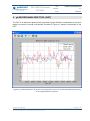
FIGURE 5-1: COMMAND LINE SCREENSHOT ............................................................................ 63
FIGURE 6-1: DAT SCREENSHOT. IT CAN BE SEEN THE POSITION ERROR FOR A PPP KINEMATIC
POSITIONING FOR A SINGLE-FREQUENCY RECEIVER. ....................................................... 64
Software User Manual
Page 5 of 69
gAGE/UPC owns the copyright of this document which shall not be used for any purpose other than for which it is supplied and shall not be copied or given
to any person or organization without written authorization from the owner.
gAGE/UPC
gAGE
Research group of Astronomy & Geomatics
Technical University of Catalonia
http://www.gage.es
ESA GNSS Education
EDUNAV
Ref.:
EDUNAV-SUM-gAGE/UPC
Iss./Rev.:
1.7
Date:
1/07/2011
1 INTRODUCTION
The GNSS-Lab Tool suite (gLAB) is an interactive educational multipurpose package to
process and analyse GNSS data. The first release of this software package allows
processing only GPS data, but it is prepared to incorporate future module updates, such as
an expansion to Galileo and GLONASS systems, EGNOS and differential processing.
This software package is targeting the following groups of users:
•
•
•
Education professionals aiming to teach GNSS from both a theoretical and practical
points of view.
Standalone students and professionals with basic knowledge on GNSS as a selflearning tool.
Professionals with more in deep knowledge on GNSS who want an easy and userfriendly tool with precise positioning capability.
From an operative point view, this tool is conceived as a software package to support a
practical GNSS course, where the fundamentals introduced in the theory are experimented
through guided exercises. In this way, the tool is conceived for being used:
•
•
•
as part of a GNSS course with practical exercises integrated following a manual, or
experimenting around with contextual help with hyperlinks for more information, or
to process RINEX data and obtain both GPS standalone or Precise Point Positioning
(PPP) solutions.
The gLAB tool is distributed within a learning material package containing the following
components:
•
•
•
Software: A binary which will be able to read GPS RINEX data, process it and
show the results in the form of data files and graphics. The processing options will
be fully parametrizable through a GUI that will ease to understand the tool and its
different options. The software is able to work both in Windows and Linux Operating
Systems.
Tutorial: A book containing the GNSS fundamentals and several practical
exercises covering from the basics of data processing, such as reading standard
RINEX format to more complex processes, as positioning a rover and analysing the
results.
Data: The data sets files used in the exercises.
1.1 DOCUMENT SCOPE AND PURPOSES
This document contains the information related to the use of the gLAB software package
component of the gLAB suite, and its purpose is to provide an overall overview to the end
user of the software. In particular, how to install it and use it, with all the different options
that the software has.
Software User Manual
Page 6 of 69
gAGE/UPC owns the copyright of this document which shall not be used for any purpose other than for which it is supplied and shall not be copied or given
to any person or organization without written authorization from the owner.
gAGE/UPC
gAGE
Research group of Astronomy & Geomatics
Technical University of Catalonia
http://www.gage.es
ESA GNSS Education
EDUNAV
Ref.:
EDUNAV-SUM-gAGE/UPC
Iss./Rev.:
1.7
Date:
1/07/2011
1.2 DOCUMENT OVERVIEW AND STRUCTURE
This document is split in sections, which describe:
•
A generic description on the different software modules included in the package
(Section 2).
•
A detailed description of the installation procedure (Section 3).
•
How to use the Graphic User Interface (GUI) component (Section 4).
•
How to use the Data Processing Core (DPC) component (Section 5).
•
How to use the Data Analysis Tool (DAT) component (Section 6).
1.3 APPLICABLE AND REFERENCE DOCUMENTS
1.3.1 Applicable documents
The following documents refer to the applicable documents for the project.
AD-01
RINEX-2.10 format: http://igscb.jpl.nasa.gov/igscb/data/format/rinex211.txt
AD-02
RINEX-3.00 format: ftp://epncb.oma.be/pub/data/format/rinex300.pdf
AD-03
IONEX format: http://igscb.jpl.nasa.gov/igscb/data/format/ionex1.pdf
AD-04
SP3 format: http://igscb.jpl.nasa.gov/igscb/data/format/sp3.txt
AD-05
RINEX clock format: http://igscb.jpl.nasa.gov/igscb/data/format/rinex_clock.txt
AD-06
ANTEX format: ftp://igscb.jpl.nasa.gov/igscb/station/general/antex13.txt
AD-07
RTCA-MOPS, December 2006.
1.3.2 Reference Documents
RD-1
Python Programming Language, http://www.python.org
RD-2
Guide to Applying the ESA Software Engineering Standards to small Software
Projects Doc.-No. ESA BSSC (96)2 Issue 1, 199.
RD-3
Gnuplot: http://www.gnuplot.info
RD-4
Architecture Design Document for gLAB, gAGE/UPC 2009.
RD-5
ANTEX file: http://igscb.jpl.nasa.gov/igscb/station/general/igs05.atx
RD-6
SP3 files: http://igscb.jpl.nasa.gov/igscb/product
RD-7
GIPSY OASIS-II, Mathematical description, 1986
Software User Manual
Page 7 of 69
gAGE/UPC owns the copyright of this document which shall not be used for any purpose other than for which it is supplied and shall not be copied or given
to any person or organization without written authorization from the owner.
gAGE
gAGE/UPC
Research group of Astronomy & Geomatics
Technical University of Catalonia
http://www.gage.es
ESA GNSS Education
EDUNAV
Ref.:
EDUNAV-SUM-gAGE/UPC
Iss./Rev.:
1.7
Date:
1/07/2011
RD-8
A. E. Niell, Global mapping functions for the atmosphere delay at radio
wavelengths, Journal of Geophysical Research, Vol. 101, No. B2, p. 32273246, 1996.
RD-9
RTCA, 2001. Minimum Operational Performance Standards For Global Positioning
Sysmte/Wide Area Augmentation System Airborne Equipment. RTCA/DO-229C.
Prepared by SC-159. November 28, 2001. Supersedes DO-229B. Available
at http://www.rtca.org/doclist.asp . pp. 338-340 of 586 in PDF.
RD-10
D. McCarthy and G. Petit, IERS Conventions, International Earth Rotation and
Reference Systems Service (IERS), 2003
RD-11
S. Malsys, M. Larezos, S. Gottschalk, S. Mobbs, B. Winn, W. Feess, M. Menn,
E. Swift, E. Merrigan and W. Mathon, The GPS accuracy improvement
initiative, ION GNSS 1997, Kansas City, USA, pp. 375-384, 1997.
RD-12
GPSConstellationStatus.txt file, available at:
http://gge.unb.ca/Resources/GPSConstellationStatus.txt
RD-13
ICD-GPS-200, Navstar GPS Space Segment / Navigation User Interfaces,
1993.
RD-14
Global Positioning System Standard Positioning Service Signal Specification.
U.S. Department of Defense, DOD 4650.5/SPSSP V3, 3rd Edition, August 1,
1998.
1.3.3 Acronyms and Terms
AD
DAT
DPC
ESA
gAGE
gLAB
GNSS
GUI
IGS
OS
PPP
RD
SIS
SOW
S/W
TBC
TBD
TBW
TGD
UD
Applicable Document
Data Analysis Tool
Data Processing Core
European Space Agency
Research Group of Astronomy and Geomatics
GNSS-Lab tool
Global Navigation Satellite System
Graphic User interface
International GNSS Service
Operative System
Precise point Positioning
Reference Document
Signal In Space
Statement Of Work
Software
To Be Confirmed
To Be Determined
To Be Written
Total Group Delay
User Domain
Software User Manual
Page 8 of 69
gAGE/UPC owns the copyright of this document which shall not be used for any purpose other than for which it is supplied and shall not be copied or given
to any person or organization without written authorization from the owner.
gAGE
gAGE/UPC
Research group of Astronomy & Geomatics
Technical University of Catalonia
http://www.gage.es
UPC
ESA GNSS Education
EDUNAV
Ref.:
EDUNAV-SUM-gAGE/UPC
Iss./Rev.:
1.7
Date:
1/07/2011
Technical University of Catalonia
Software User Manual
Page 9 of 69
gAGE/UPC owns the copyright of this document which shall not be used for any purpose other than for which it is supplied and shall not be copied or given
to any person or organization without written authorization from the owner.
gAGE/UPC
gAGE
Research group of Astronomy & Geomatics
Technical University of Catalonia
http://www.gage.es
ESA GNSS Education
EDUNAV
Ref.:
EDUNAV-SUM-gAGE/UPC
Iss./Rev.:
1.7
Date:
1/07/2011
2 gLAB SOFTWARE TOOL
The gLAB software tool is able to run under Linux and Windows operating systems (OS). It
is programmed in ANSI C and Python languages and contains three main software
modules:
•
Data Processing Core (DPC) [gLAB.exe in Windows, gLAB_linux for Linux]
•
Graphic User Interface (GUI) and [gLAB_GUI.exe in Windows, gLAB_GUI.py in
Linux]
•
Data Analysis Tool (DAT) [graph.exe in Windows, graph.py in Linux].
The DPC implements all the data processing algorithms and can be executed either, in
command line or with the GUI. The GUI consists in different graphic panels for a user
friendly managing of the SW and the tool configuration. They provide all the options to
configure the model and navigation. The Data Analysis Tool provides a user friendly
environment for the data analysis and results visualizing.
The tool contains a precise modelling of the GNSS observables (code and phase) at the
centimetre level, allowing both standalone GPS positioning and PPP. The software is ready
to incorporate future updates to Galileo or GLONASS systems.
2.1.1 Software package features
•
Graphic User Interface (GUI) to ease the utilisation of the tool with most of the
capabilities of the DPC. The GUI allows a high customisation interface to process a
wide range of options.
•
Tooltips in the GUI, which allow understanding and using the different options.
•
Capable to read:
o
Station measurements from Observation RINEX standard 2.11.
o
Station measurements from Observation RINEX standard 3.00.
o
Broadcast message from Navigation RINEX standard.
o
Satellite clocks from Clocks RINEX standard.
o
Satellite orbits and clocks from SP3 standard.
o
Ionospheric maps from IONEX standard.
o
Constellation status (with information between Satellite Vehicle Number
(SVN) and PRN) of the satellite.
o
Antenna Phase Center information from ANTEX standard.
o
Differential Code Biases from precise .DCB files.
o
Receiver type information from GPS Receiver File Types,
Software User Manual
Page 10 of 69
gAGE/UPC owns the copyright of this document which shall not be used for any purpose other than for which it is supplied and shall not be copied or given
to any person or organization without written authorization from the owner.
gAGE/UPC
gAGE
Research group of Astronomy & Geomatics
Technical University of Catalonia
http://www.gage.es
ESA GNSS Education
EDUNAV
Ref.:
EDUNAV-SUM-gAGE/UPC
Iss./Rev.:
1.7
Date:
1/07/2011
•
The DPC is able to work both with command-line parameters and a configuration
file.
•
Automatically detects if the format is RINEX 2.11 or 3.00.
•
Fully capable to read Galileo (and other constellations) from RINEX.
•
Able to process both pseudorange and carrier phase.
•
Detection of cycle-slips in carrier phase measurements for GPS with three different
methods:
o
Geometric-free carrier phase combination.
o
Melbourne-Wübbena combination.
o
Code-Phase difference (for single-frequency receivers),
•
Time handling routines (The native time format of the software is Modified Julian
Day and seconds of day).
•
Prealignment of carrier phase to pseudorange measurements. This is done to avoid
large differences between both kinds of measurements, and allow a more direct
comparison. The alignment is done keeping the integer part of the carrier phase.
•
Pseudorange jump checking. Some receivers have an inconsistent set of
pseudorange and carrier phase measurements when they adjust their own clock
(doing one or more leap miliseconds). Their pseudorange measurements are
consistent with this change in clock, but carrier phases do not show it. This creates
an inconsistency and a general cycle-slip for all satellites if not handled properly.
gLAB detects and corrects this problem.
•
Decimation capabilities. gLAB can decimate the input RINEX to increase
computation speed if a high sampling rate is not needed. The decimation comes
after the cycle-slip detection to take full profit of the input data rate.
•
Able to individually select/deselect each satellite for processing.
•
Able to set an elevation mask to ignore low satellites for processing.
•
Able to specifically mark which frequencies are available (to simulate singlefrequency receivers from dual-frequency RINEX data).
•
Pseudorange smoothing option.
•
Orbit interpolation of SP3 data.
•
Broadcast message support (orbit estimation, clock correction, TGD correction).
•
Orbit/Clock comparison mode (it can compare the orbit and clocks from 2 different
sources, i.e. broadcast, SP3 and clocks files).
•
Sun approximate positioning (for satellite orientation).
•
Models implemented (all of them can be enabled or disabled):
o
Satellite clock error correction.
o
Transmission time computation.
Software User Manual
Page 11 of 69
gAGE/UPC owns the copyright of this document which shall not be used for any purpose other than for which it is supplied and shall not be copied or given
to any person or organization without written authorization from the owner.
gAGE/UPC
gAGE
Research group of Astronomy & Geomatics
Technical University of Catalonia
http://www.gage.es
ESA GNSS Education
EDUNAV
Ref.:
EDUNAV-SUM-gAGE/UPC
Iss./Rev.:
1.7
Date:
1/07/2011
o
Earth rotation in flight time of the signal.
o
Satellite phase center correction.
o
Receiver phase center correction.
o
Receiver Antenna Reference Point (ARP) correction.
o
Relativistic correction.
o
Klobuchar ionospheric correction.
o
Tropospheric correction [one simple model and the more refined Niell
mapping model]
o
P1 – P2 Differential Code Bias (DCB) correction.
o
P1 – C1 Differential Code Bias (DCB) correction.
o
Wind up effect.
o
Solid tides correction.
o
Gravitational delay correction [an effect of general relativity due to the gravity
field gradient between receiver and transmitter].
•
Able to choose different measurements (1 or more) for the filter estimation (both
carrier phase and pseudorange). It could even work with a set of different
pseudorange measurements from different signals. This can be useful in the future
Galileo scenario, where some processing with different measurements can be
desired.
•
Able to assign different weights for different measurements.
•
Able to assign elevation dependant weights.
•
Able to translate from cartesian (native of the software) to geodetic coordinates.
•
Orientation estimation of both the satellites and the receiver (and thence the
azimuth/elevation of the receiver-satellite pair).
•
Standalone processing using broadcast and C/A code (fully configurable to be able
to used also carrier phase if required).
•
Precise Point Positioning (PPP) with precise orbit and clocks, precise models and
Pc/Lc measurements (ionospheric-free combinations). It is also fully configurable.
•
Able to create different plots to visualise the data processed.
•
Detection and warning of convergence problems.
2.1.2 Identified limitations
The current version gLAB only implements full processing capabilities for GPS data.
Nevertheless, the reading of RINEX-3.00 Galileo and GLONASS data functionality
Software User Manual
Page 12 of 69
gAGE/UPC owns the copyright of this document which shall not be used for any purpose other than for which it is supplied and shall not be copied or given
to any person or organization without written authorization from the owner.
gAGE/UPC
gAGE
Research group of Astronomy & Geomatics
Technical University of Catalonia
http://www.gage.es
ESA GNSS Education
EDUNAV
Ref.:
EDUNAV-SUM-gAGE/UPC
Iss./Rev.:
1.7
Date:
1/07/2011
is also included, allowing performing some exercises on data analysis with real or
simulated Galileo and GLONASS measurements.
2.1.3 Minimum hardware requirements
gLAB requires the following computer minimum hardware requirements in order to be
properly executed:
•
256 MB of memory.
•
CPU with at least 1GHz.
•
200MB of hard disk free space.
•
Screen resolution of at least 1024x768 is recommended. In order to cope with
potential users using small screens, scrollbars can be displayed in the preferences
button.
2.1.4 Minimum software requirements
The program runs under Windows XP and Linux Operating systems.
2.1.4.1 Windows
No specific software is required to execute the program in Windows XP.
For Windows Vista users, it is necessary to generate new binaries for gLAB (as explained is
section 3.1.1). In this sense, the following programs are required:
•
MinGW v5.1.4 (http://sourceforge.net/projects/mingw/files/)
•
Python(x,y) v2.1.14 (http://www.pythonxy.com). During its installation please select
as “type of install”: Full.
2.1.4.2 Linux
For Linux users, the following programs are required (later versions may also work):
•
make 3.81
•
gcc 4.1.3
•
Python v2.5.4
•
wxPython v2.8.9.2
•
Python matplotlib v0.98.5.4
Software User Manual
Page 13 of 69
gAGE/UPC owns the copyright of this document which shall not be used for any purpose other than for which it is supplied and shall not be copied or given
to any person or organization without written authorization from the owner.
gAGE/UPC
gAGE
Research group of Astronomy & Geomatics
Technical University of Catalonia
http://www.gage.es
•
ESA GNSS Education
EDUNAV
Ref.:
EDUNAV-SUM-gAGE/UPC
Iss./Rev.:
1.7
Date:
1/07/2011
Python Tkinter v5.4.0
Software User Manual
Page 14 of 69
gAGE/UPC owns the copyright of this document which shall not be used for any purpose other than for which it is supplied and shall not be copied or given
to any person or organization without written authorization from the owner.
gAGE/UPC
gAGE
Research group of Astronomy & Geomatics
Technical University of Catalonia
http://www.gage.es
ESA GNSS Education
EDUNAV
Ref.:
EDUNAV-SUM-gAGE/UPC
Iss./Rev.:
1.7
Date:
1/07/2011
3 INSTALLATION PROCEDURE
The gLAB software package can be downloaded from the following URL:
http://www.gage.es/gLAB/
In this web page it is possible to download the last version of gLAB both in Windows and
Linux.
3.1 WINDOWS XP AND VISTA
The installation of the Windows version is initiated by executing the installation program.
During the installation process you have several configurable options, such as the
installation directory (by default, C:\Program Files\gLAB), and the possibility to create
shortcuts.
The installation will create a gLAB group in the start menu with the following elements:
•
gLAB on the Web, will forward to the webpage of gLAB.
•
Uninstall gLAB, to completely remove gLAB from the computer.
•
gLAB_GUI, the Graphic User Interface of gLAB.
•
Command line in directory, which will open a new command line window in the
directory gLAB was installed.
Executing the gLAB_GUI option will run the GUI program.
3.1.1 Manual binary generation
All the binaries of the Windows XP version of gLAB have been precompiled, so no need to
compile them again would be required. In the case that the source code is modified, or in
the case that some of the binaries are not properly working a manual binary generation
would be needed. Windows Vista has some problems with the precompiled version of XP,
so this procedure should be applied to Windows Vista users.
For the manual binary generation the following programs need to be installed (other
versions may also work):
•
MinGW v5.1.4 (http://sourceforge.net/projects/mingw/files/)
•
Python(x,y) v2.1.14 (http://www.pythonxy.com). During its installation please select
as “type of install”: Full.
Once these programs have been installed, the script “createEXE.bat” can be executed. This
script can be found in the installation directory of gLAB, and will compile everything and
create the proper binaries.
Software User Manual
Page 15 of 69
gAGE/UPC owns the copyright of this document which shall not be used for any purpose other than for which it is supplied and shall not be copied or given
to any person or organization without written authorization from the owner.
gAGE/UPC
gAGE
Research group of Astronomy & Geomatics
Technical University of Catalonia
http://www.gage.es
ESA GNSS Education
EDUNAV
Ref.:
EDUNAV-SUM-gAGE/UPC
Iss./Rev.:
1.7
Date:
1/07/2011
3.2 LINUX
gLAB has been successfully tested under Ubuntu, but should work in other Linux
distributions.
The Linux version of gLAB has to be decompressed to a directory, using the following
command:
tar –xvzf glab_vx.x.tgz
This will create a directory called ‘gLAB’ with all the program structure. Next, it is necessary
to compile the DPC, for this:
cd gLAB
make –f makefile_linux
This will create the binary for the DPC of gLAB (gLAB_linux).
In order to be able to launch the python programs (GUI and DAT), it is necessary to have
the following packets installed in the system (other versions may also work):
•
Python v2.5.4
•
wxPython v2.8.9.2
•
Python matplotlib v0.98.5.4
•
Python Tkinter v5.4.0
In ubuntu, this can easily be done by using the following command:
apt-get install python python-wxtools python-matplotlib python-tk
3.3 DIRECTORY STRUCTURE
gLAB
gLAB/src
gLAB/test
gLAB/win
The gLAB directory contains all the binaries, python programs and other files.
The gLAB/src directory contains the C source code of the DPC.
The gLAB/win (only available in the windows distribution) directory contains all the required
data for the GUI and DAT binaries. This directory can be fully generated by the “Manual
binary generation” procedure set above.
The gLAB/test directory contains a set of test files to be used with the gLAB program.
Software User Manual
Page 16 of 69
gAGE/UPC owns the copyright of this document which shall not be used for any purpose other than for which it is supplied and shall not be copied or given
to any person or organization without written authorization from the owner.
gAGE/UPC
gAGE
Research group of Astronomy & Geomatics
Technical University of Catalonia
http://www.gage.es
ESA GNSS Education
EDUNAV
Ref.:
EDUNAV-SUM-gAGE/UPC
Iss./Rev.:
1.7
Date:
1/07/2011
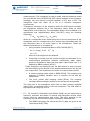
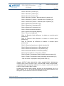
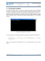
4 gLAB GRAPHIC USER INTERFACE (GUI)
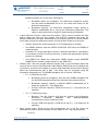
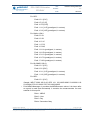
4.1 THE BASICS
The GUI is an interface between the other two components, the DPC and the DAT. It will
allow the user changing different parameters, and execute the other two programs with the
proper arguments. The initial screen of the GUI can be seen in Figure 4-1.
Figure 4-1: Initial screen of the gLAB Graphic User Interface
Two main tabs can be found:
•
Positioning: This tabs interfaces with the DPC tool, and allows selecting all the
different processing options.
•
Analysis: This tabs interfaces with the DAT tool, and allows selecting all the different
plotting options.
Software User Manual
Page 17 of 69
gAGE/UPC owns the copyright of this document which shall not be used for any purpose other than for which it is supplied and shall not be copied or given
to any person or organization without written authorization from the owner.
gAGE/UPC
gAGE
Research group of Astronomy & Geomatics
Technical University of Catalonia
http://www.gage.es
ESA GNSS Education
EDUNAV
Ref.:
EDUNAV-SUM-gAGE/UPC
Iss./Rev.:
1.7
Date:
1/07/2011
The following sections will provide in-deep information on the different options of the GUI.
Most of the information here can also be found with the inline tooltips. On the top of the
screen two different buttons can be found:
•
Preferences: Allows to select/deselect explanatory tooltips (selected by default), to
select/deselect scrollbars, and to check for new updates of the tool.
Figure 4-2: Preferences Frame
•
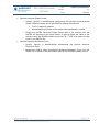
About: General information on the tool.
Software User Manual
Page 18 of 69
gAGE/UPC owns the copyright of this document which shall not be used for any purpose other than for which it is supplied and shall not be copied or given
to any person or organization without written authorization from the owner.
gAGE/UPC
gAGE
Research group of Astronomy & Geomatics
Technical University of Catalonia
http://www.gage.es
ESA GNSS Education
EDUNAV
Ref.:
EDUNAV-SUM-gAGE/UPC
Iss./Rev.:
1.7
Date:
1/07/2011
Figure 4-3: About Frame
4.2 CALCULUS (DPC INTERFACE)
The calculus tab is split into 5 different sections, which correspond to 5 different modules
inside the DPC (see the Architecture Design Document for gLAB RD-4). The different
modules of the DPC are:
•
DATAHANDLING module: It is the storage of the data. This module does not appear
in the GUI interface, because it has no configuration options. It defines all the
structures and enumerators of the program and has functions to access the data.
•
INPUT module: It can be understand as a "driver" between the input data and the
rest of the program. This module implements all the input reading capabilities and
stores it in structures defined in the DATAHANDLING module.
•
PREPROCESS module: This module process the data before the MODEL. It checks
for cycle-slips, pseudorange-carrier phase inconsistencies and decimates the data (if
requiered).
Software User Manual
Page 19 of 69
gAGE/UPC owns the copyright of this document which shall not be used for any purpose other than for which it is supplied and shall not be copied or given
to any person or organization without written authorization from the owner.
gAGE/UPC
gAGE
Research group of Astronomy & Geomatics
Technical University of Catalonia
http://www.gage.es
ESA GNSS Education
EDUNAV
Ref.:
EDUNAV-SUM-gAGE/UPC
Iss./Rev.:
1.7
Date:
1/07/2011
•
MODEL module: This module has all the functions to fully model the receiver
measurements. As said, it implements several kind of models, which can be
activated or desactivated.
•
FILTER module: This module implements an Extended Kalman Filter (EKF) fully
configurable, and obtains the estimations of the required parameters.
•
OUTPUT module: This module outputs the data obtained from the FILTER.
Software User Manual
Page 20 of 69
gAGE/UPC owns the copyright of this document which shall not be used for any purpose other than for which it is supplied and shall not be copied or given
to any person or organization without written authorization from the owner.
gAGE/UPC
gAGE
Research group of Astronomy & Geomatics
Technical University of Catalonia
http://www.gage.es
ESA GNSS Education
EDUNAV
Ref.:
EDUNAV-SUM-gAGE/UPC
Iss./Rev.:
1.7
Date:
1/07/2011
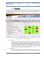
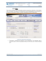
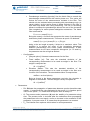
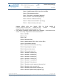
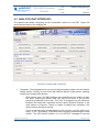
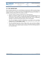
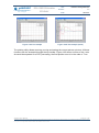
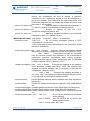
4.2.1 Input
This section provides all the configuration options to select the input files for gLAB.
Figure 4-4: Screenshot of the INPUT section.
•
•
Default Templates: Configure all the options of the program for a specific
processing:
o
SPS Template: Selects all the options to perform a Standard Positioning
Service (SPS) processing.
o
PPP Template: Selects all the options to perform a Precise Point Positioning
(PPP) processing for the computation of precise coordinates.
Input files: Section to include all the files required for the proper functioning of the
program.
o
RINEX Observation File: Source GNSS measurements data file in RINEX
format (version 2.11 or 3.00).
Software User Manual
Page 21 of 69
gAGE/UPC owns the copyright of this document which shall not be used for any purpose other than for which it is supplied and shall not be copied or given
to any person or organization without written authorization from the owner.
gAGE
gAGE/UPC
Research group of Astronomy & Geomatics
Technical University of Catalonia
http://www.gage.es
ESA GNSS Education
EDUNAV
Ref.:
EDUNAV-SUM-gAGE/UPC
Iss./Rev.:
1.7
Date:
1/07/2011
o
ANTEX File: Antenna phase center information for both GNSS satellites and
receiver antennas 1.
o
Orbit and Clock Source: Origin of the orbit and clock products. The option
selected here must be consistent with the Navigation Mode in the Filter
section: Broadcast => Standalone, Precise (1 file) or Precise (2 files) => PPP
o

Broadcast: RINEX navigation file with the broadcasted message
[Standalone option must be marked in the Filter section].

Precise (1 file): SP3 format file with the position/clock errors of GNSS
satellites for a set of specific timestamps [PPP option must be marked
in the Filter section] 2.

Precise (2 files): The source of orbits will be an SP3 format file, and
the clocks will be a RINEX clock format. While orbit data can be
interpolated without much data degradation, clocks cannot be. The
RINEX clock format allows providing clocks at a high rate, while
reading the orbits at a lower rate from the SP3 file [PPP option must
be marked in the Filter section].
•
Orbits SP3 File: Source of orbit data.
•
Clocks Rinex File: Source of clock data.
Ionosphere Source: Origin of the ionosphere data when correcting it (see the
1
The last ANTEX files can be found in: [RD-5]. The gLAB suite includes two different
ANTEX files: igs05.atx and igs_pre1400.atx. The first file is directly downloaded from [RDth
5], and should be used for data sets after GPS week 1400 (5 of November of 2006). The
second one should be used before this date. This is because there was a change in the
way that Satellite Phase Centers were obtained. Thence using Precise files for navigation
with the incorrect set of ANTEX file will be translated in higher than expected errors.
2
SP3 files can be found at the IGS site: [RD-6].
Software User Manual
Page 22 of 69
gAGE/UPC owns the copyright of this document which shall not be used for any purpose other than for which it is supplied and shall not be copied or given
to any person or organization without written authorization from the owner.
gAGE/UPC
gAGE
Research group of Astronomy & Geomatics
Technical University of Catalonia
http://www.gage.es
ESA GNSS Education
EDUNAV
Ref.:
EDUNAV-SUM-gAGE/UPC
Iss./Rev.:
1.7
Date:
1/07/2011
Modeling section (4.2.3) for more information).
•
•
Broadcast (same as navigation): For Klobuchar ionospheric model,
use the same broadcasted file as for the orbits and clocks for the
Klobuchar parameters.

Broadcast (specify): For Klobuchar ionospheric model, specify a
different broadcasted file to use for the Klobuchar parameters. This
option is also useful when using SP3 and correcting ionosphere.
A priori Receiver Position: Initial receiver position. This is used to linearize the filter
and to obtain the values for the models. The OUTPUT message type gives the
position obtained by the filter differenced with this apriori position. So if this position
is accurate enough, the difference can be used as a direct measure of the error.
o
Specify: Specify the receiver position in XYZ components (in meters).
o
Use RINEX Position: Use the APROX POSITION XYZ field of the RINEX of
measurements.
o
Calculate: Do not provide apriori position, gLAB will calculate it, and adjust it
as necessary (useful for moving receivers, or when the approximate receiver
position is unknown).
o
Use SINEX File: Match the observation RINEX header record MARKER
NAME with the marker position present in the SINEX file.
Auxiliary files: User can provide different auxiliary files: to get information about the
receiver and to correct the Differential Code Biases (DCB) which are the delays due
to electronic, antennas and cables of receiver and transmitter devices which directly
affect the measurements with a bias. This effect can be corrected using the
information extracted from: The RINEX Navigation file or Precise .DCB files.
o
o
•

P1 – P2 DCB Source files:

Broadcast (same as navigation): Use the same RINEX navigation file
for the DCB computations than the orbit and clock product source.

Broadcast (specify): Specify a different RINEX broadcasted file to
obtain the codes (P1 – P2) digital bias.

Precise .DCB file: Specify a .DCB file for the (P1 – P2) biases for all
satellites.
P1 – C1 DCB Source files:

Receiver Type file: Specify a file with the receiver type information:
Receivers,
Antennas,
Radomes,
and
Antenna+Radome
manufacturer's name, model and code.

Precise .DCB files Specify a .DCB file for the (P1 – C1) biases for all
satellites.
Save Config button: Stores all the GUI configuration into a .cfg file, which can
afterwards be read by the processing core by means of the ‘-inpu:cfg’ parameter.
In Linux:
Software User Manual
Page 23 of 69
gAGE/UPC owns the copyright of this document which shall not be used for any purpose other than for which it is supplied and shall not be copied or given
to any person or organization without written authorization from the owner.
gAGE/UPC
gAGE
Research group of Astronomy & Geomatics
Technical University of Catalonia
http://www.gage.es
ESA GNSS Education
EDUNAV
Ref.:
EDUNAV-SUM-gAGE/UPC
Iss./Rev.:
1.7
Date:
1/07/2011
./gLAB_linux –input:cfg gLAB.cfg
In Windows:
gLAB.exe –input:cfg gLAB.cfg
•
Show Config button: Opens a text editor to show the stored GUI configuration file.
•
RUN button: Execute the DPC program with all the configured parameters of the
Calculus tab. This button can be used in all Input, Preprocess, Modeling, Filter and
Output sections.
•
Show Output button: Opens a text editor of the output of the last execution of gLAB.
Software User Manual
Page 24 of 69
gAGE/UPC owns the copyright of this document which shall not be used for any purpose other than for which it is supplied and shall not be copied or given
to any person or organization without written authorization from the owner.
gAGE/UPC
gAGE
Research group of Astronomy & Geomatics
Technical University of Catalonia
http://www.gage.es
ESA GNSS Education
EDUNAV
Ref.:
EDUNAV-SUM-gAGE/UPC
Iss./Rev.:
1.7
Date:
1/07/2011
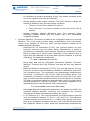
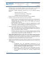
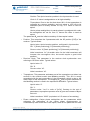
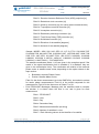
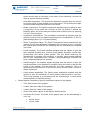
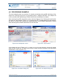
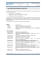
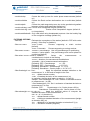
4.2.2 Preprocess
This section provides all the configuration options to preprocess the input data. In particular,
it allows changing the decimation rate, the elevation mask, the cycle-slip detection, and
selecting individual satellites for the processing. Figure 4-5 shows a screenshot of the
PREPROCESS section.
Figure 4-5: Preprocess section screenshot.
•
Station Data.
o
•
Data Decimation [s]: This option will decimate the input data at the specified
rate [in seconds]. If this option is unchecked, every time an epoch is found in
the input RINEX observation file, all the processing takes place. If this option
is checked, the data is decimated and not even modeled. Even in decimated
data, all the epochs are used for cycle slip detection, and arc length
computations, but the process is stopped just before the modeling. This
option is meant to be used to reduce computation time.
Satellite options.
o
Elevation Mask [Degrees]: The elevation mask parameter is used to discard
all the satellites below the specified elevation. Low elevation satellites should
Software User Manual
Page 25 of 69
gAGE/UPC owns the copyright of this document which shall not be used for any purpose other than for which it is supplied and shall not be copied or given
to any person or organization without written authorization from the owner.
gAGE/UPC
gAGE
Research group of Astronomy & Geomatics
Technical University of Catalonia
http://www.gage.es
ESA GNSS Education
EDUNAV
Ref.:
EDUNAV-SUM-gAGE/UPC
Iss./Rev.:
1.7
Date:
1/07/2011
be discarded for geodetic processing as they may contain increased errors
due to low signal-to-noise ratio and multipath.
o
o
•
Discard satellites under eclipse condition: This option allows to activate the
discard of satellites if they are under eclipse conditions:

They do not have direct visibility of the Sun or

They have been in the former condition at some time of the last 30
minutes.
Discard unhealthy satellites (Broadcast only): This parameter allows
discarding satellites based upon the healthy flag of the broadcasted
navigation message.
Cycle-slip Detection: This section provides all the configuration options for cycle-slip
detection. This is only used for carrier phase measurements, and in the present
version of the software for GPS only. Each cycle-slip detection method can be
enabled/disabled individually.
o
Geometric-free CP Combination [F1-F2]: This cycle-slip detector for dualfrequency receivers uses only carrier phase measurements. It creates a
geometric-free combination (which shall be affected by ionosphere) and will
follow its shape with a second order interpolator. If the expected value is
higher than the measured one by more than a specific threshold, a cycle-slip
is declared. The threshold is obtained as:
Th = max - (max-min)*exp(-step/T0)
Being max, min and T0 configurable parameters (Minimum Threshold,
Maximum Threshold and Time Constant), and step the time step between
epochs.
o
Melbourne-Wübbena Combination [F1-F2]: This cycle-slip detector for dualfrequency receivers uses the Melbourne-Wübbena combination (geometricfree ionospheric-free). This combination uses pseudorange measurements,
and thence, is affected by code receiver noise and multipath effects. This
combination is basically a constant with noise and jumps due to the cycleslips. A mobile mean and standard deviation of the last epochs is computed.
The mean is compared against the measured value, and if it is higher than a
specified threshold, a cycle-slip is declared. The threshold depends on the
standard deviation of the last epochs, and is computed as:
Th = minimum(max,maximum(k·stdDev,min))
being max, min and k configurable parameters (see below) and stdDev the
computed standard deviation. minimum() and maximum() are functions
returning the minimum and maximum between two values.
o
L1-C1 Difference [F1]: This cycle-slip detector for single-frequency receivers
uses the difference between L1 and C1 (L1P and C1C). This difference
contains basically noise coming from C1, sudden jumps coming from cycleslips, and a ionospheric divergence with time, due to the different effects that
the ionosphere causes in carrier phase and pseudorange measurements.
Software User Manual
Page 26 of 69
gAGE/UPC owns the copyright of this document which shall not be used for any purpose other than for which it is supplied and shall not be copied or given
to any person or organization without written authorization from the owner.
gAGE/UPC
gAGE
Research group of Astronomy & Geomatics
Technical University of Catalonia
http://www.gage.es
ESA GNSS Education
EDUNAV
Ref.:
EDUNAV-SUM-gAGE/UPC
Iss./Rev.:
1.7
Date:
1/07/2011
This detector computes the mean and standard deviation of L1-C1 along the
epochs, proving a window to limit the divergence. The expected mean value
is compared against the obtained one, and if it is higher than a specific
threshold, a cycle-slip is declared. The threshold is obtained as:
Th = minimum(k·stdDev,max)
being k, max and the window size configurable parameters, stdDev the
computed standard deviation, and minimum() the function returning the
minimum between two values.
•
GNSS Satellite Selection: The buttons allow to individually select/deselect each
satellite for processing. A deselected satellite shall not be taken into account when
processing. Green color marks selected satellites and red deselected satellites.
Software User Manual
Page 27 of 69
gAGE/UPC owns the copyright of this document which shall not be used for any purpose other than for which it is supplied and shall not be copied or given
to any person or organization without written authorization from the owner.
gAGE/UPC
gAGE
Research group of Astronomy & Geomatics
Technical University of Catalonia
http://www.gage.es
ESA GNSS Education
EDUNAV
Ref.:
EDUNAV-SUM-gAGE/UPC
Iss./Rev.:
1.7
Date:
1/07/2011
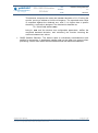
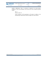
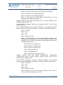
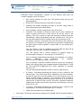
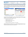
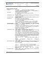
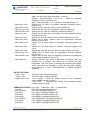
4.2.3 Modeling
This section provides the configuration options to set/unset each individual model that is
used by gLAB. Figure 4-6 shows a screenshot of the MODEL section.
Figure 4-6: Modeling section screenshot
•
Modeling Options: The following options allow to enable/disable the different models
included in the processing.
o
Satellite clock offset correction: The satellite clock errors correspond to the
clock synchronism errors of the satellite clocks in relation to the GNSS
system time scale. These errors depend heavily on the type of oscillator of
the satellite and are quite unpredictable. They can only be obtained by some
kind of estimation. The typical source for estimations of these errors are the
own navigation message, or some kind of external estimation, such as SP3
files. The effect of these clock errors can reach up hundreds of kilometers.
o
Consider satellite movement during signal flight time: Due to the distance
between satellites and receivers (between 20000 and 26000 Km for GPS),
the signal travel time is not despicable (about 70 ms for GPS). Thence the
receiver is obtaining the measurement after it has been emitted by the
Software User Manual
Page 28 of 69
gAGE/UPC owns the copyright of this document which shall not be used for any purpose other than for which it is supplied and shall not be copied or given
to any person or organization without written authorization from the owner.
gAGE
gAGE/UPC
Research group of Astronomy & Geomatics
Technical University of Catalonia
http://www.gage.es
ESA GNSS Education
EDUNAV
Ref.:
EDUNAV-SUM-gAGE/UPC
Iss./Rev.:
1.7
Date:
1/07/2011
satellite. This fact should be taken into consideration, as the position of the
satellite must be computed in the transmission time, not in the reception time.
This effect can impact on the measurements up to hundreds of meters.
o
Consider Earth rotation during signal flight time: Besides the satellite
movement during signal flight time, the Earth also moves [rotates]. If this
effect is not taken into consideration, an error of about 30 m in the east
direction would be seen.
o
Satellite mass center to antenna phase center correction: Each data source
of satellite orbits (in general the navigation message or an SP3 file) provides
these orbits in its specific reference. In particular, the SP3 files provide the
positions of the satellite referred to its mass center (which is different than
the antenna phase centers). In order to properly correct the GNSS
measurements with the satellite position, a correction between these two
centers must be done. Usually these corrections can be obtained from an
ANTEX file. This error can be up to 1-2 m. The positions computed from the
navigation message do not require any additional corrections, as they are
referred to the antenna phase center.
o
Receiver antenna phase center correction: Normally the positions of the
stations are given in relation to the base of the station. The difference
between this point and the antenna phase center should be taken into
account. This effect depends on the frequency, and can reach up to some
decimetres.
o
Receiver antenna reference point correction: Additionally to the Antenna
Phase Center, the position of a station can be given in relation to a specific
point (such as a geodetically positioned point in the ground). This correction
allows to give a specific correction to the position in North/East/Up
components.
o
Relativistic clock correction: The rate of advance of two identical clocks, one
placed in the satellite and the other on the terrestrial surface, will differ due to
the difference of the gravitational potential (general relativity) and to the
relative speed between them (special relativity). The special relativity
difference can be broken into (Hofmann-Wellenhof): 1) A constant
component that only depends on the nominal value of the semi-major axis of
the satellite orbit, which is adjusted modifying the clock oscillating frequency
of the satellite. 2) A periodical component due to the orbit eccentricity (that
must be adjusted by the user receiver) equal to:
rel = 2*(r·v)/c
This effect can reach up to 13 m.
o
Ionospheric correction: The ionosphere is the zone of the terrestrial
atmosphere that extends itself from about 60 km until more than 2000 km
high. Due to the interaction with free electrons, electromagnetic signals that
go through it suffer a delay/advancement in relation to the propagation in a
vacuum. This effect is a dispersive effect (frequency dependent), and can be
removed in multi-frequency receivers (with a specific combination of
Software User Manual
Page 29 of 69
gAGE/UPC owns the copyright of this document which shall not be used for any purpose other than for which it is supplied and shall not be copied or given
to any person or organization without written authorization from the owner.
gAGE
gAGE/UPC
Research group of Astronomy & Geomatics
Technical University of Catalonia
http://www.gage.es
ESA GNSS Education
EDUNAV
Ref.:
EDUNAV-SUM-gAGE/UPC
Iss./Rev.:
1.7
Date:
1/07/2011
measurements). The ionosphere is hard to model, and the Klobuchar model
(the one defined in the GPS/SPS-SS [RD-14] and available in the navigation
message) can only reduce its impact between a 50% and a 60%. The
ionosphere effect can reach up to 50 m in turbulent ionospheric
environments.
o
Tropospheric correction: At the frequency which the GPS signal is emitted,
the troposphere behaves like a non dispersive media, being its effect
independent of the frequency. The tropospheric delay can be modelled in an
approximate way (approximately about 90%-95%) using the following
expression:
T = ddry · mdry(elev) + dwet · mwet(elev)
where ddry corresponds to the vertical delay due to the dry component of the
troposphere and dwet corresponds to the vertical delay associated with the
wet component (due to the water vapor of the atmosphere). These two
different nominals can ve computed as

Using a simple nominal described in GIPSY-OASIS [RD-7]:
ddry = 2.3 exp (−0.116 · 10−3 · H)
dwet = 0.1
where H is the height over the ellipsoid.

Computing a nominal from the receiver’s height and estimates of five
meteorological parameters: pressure, temperature, water vapour
pressure, temperature lapse rate and water vapour lapse rate. It is
adopted by SBAS systems (AD-07).
Finally mdry(elev) and mwet(elev) are the slant factors in order to project
the vertical delay in the direction of the satellite observation for the dry and
wet components. Two models can be chosen to compute these m(elev):

A simple mapping model (used in SBAS [RD-9]). This mapping only
depends on satellite elevation and it is common for wet and dry
components.

The more refined Niell mapping model [RD-8]. This mapping
considers different obliquity factors for the wet and dry components.
The main part of the troposphere which has not been properly modelled
(about 10%) corresponds mainly to the wet component. The total effect of
troposphere can range up to 10 m.
o
P1 – P2 correction: Differential Code Biases (DCB) are the delays due to
electronic, antennas and cables of receiver and transmitter devices which
directly affect the measurements with a bias. This effect depends on the
frequency and can be corrected using the information extracted from:

Software User Manual
The RINEX Navigation file, where the (P2-P1) bias are given as the
Total Group Delay (TGD).
Page 30 of 69
gAGE/UPC owns the copyright of this document which shall not be used for any purpose other than for which it is supplied and shall not be copied or given
to any person or organization without written authorization from the owner.
gAGE/UPC
gAGE
Research group of Astronomy & Geomatics
Technical University of Catalonia
http://www.gage.es

o
•
ESA GNSS Education
EDUNAV
Ref.:
EDUNAV-SUM-gAGE/UPC
Iss./Rev.:
1.7
Date:
1/07/2011
Precise .DCB files, where the International GNSS Service (IGS) gives
an accurate estimation of the (P1-P2) bias. This file contains a
monthly estimation of this bias for all Satellites
P1 – C1 DCB correction: Differential Code Biases (DCB) are the delays due
to electronic, antennas and cables of receiver and transmitter devices which
directly affect the measurements with a bias. Because the code generation
depends on the Receiver Type, this receiver-related information has to be
given together with the corrections. gLAB works in two different modes:

Flexible: gLAB will use whichever C1 or P1 measurement is available
in the receiver, without correcting DCB. If both code measures are
available, P1 will be used as default. Used when receiver provides C1
but P1 is missing (or viceversa).

Strict: gLAB Data Processing Core (DPC) stops if both files are not
provided:
•
Receiver Type File: To identify how codes are generated in
the receiver, and how to remove these C1-P1 biases.
•
P1-C1 DCB File : Containing the P1-C1 DCB corrections.
o
Wind up correction (Carrier phase only): The wind up only appears in carrier
phase measurements and is due to the rotation of the Line-of-sight vector in
relation to the antenna. The wind-up has an accumulative effect, and for
fixed antennas can reach up to half the wave length of the measurement.
o
Solid tides correction: The attraction of Sun and Moon and the inelasticity of
the Earth's mantle cause variations to the positions of ground receivers. This
effect can reach up to some decimetres (the model used is described in [RD10], and is implemented up to degree 3).
o
Relativistic path range correction: As introduced in the Relativistic clock
correction section, the difference of the gravitational potential (general
relativity) affects the measurement. This is a small effect that has elevation
dependence, and has a total effect of about 4 cm.
Precise Products Data Interpolation: This is the degree of the interpolation
polynomial for the precise orbit and clocks (this option has no effect when using
broadcasted products).
o
Orbit Interpolation Degree: By default, the interpolation is done with a
polynomial of degree 9, but this value can be adjusted with this parameter.
Excessively low values would strongly affect the precision of the position
obtained.
o
Clock Interpolation Degree: By default, no interpolation is done ("degree" 0),
but you can chose to activate the interpolation by providing a number
different than 0. Due to the unpredictability of clocks, and its non-smoothed
nature, the interpolation of low sampling rate clocks (i.e., t>30 secs) would
strongly affect the precision of the clocks obtained. Only clocks with sampling
rate higher than 1/30s should be interpolated with a polynomial of degree 1.
Software User Manual
Page 31 of 69
gAGE/UPC owns the copyright of this document which shall not be used for any purpose other than for which it is supplied and shall not be copied or given
to any person or organization without written authorization from the owner.
gAGE/UPC
gAGE
Research group of Astronomy & Geomatics
Technical University of Catalonia
http://www.gage.es
•
Ref.:
EDUNAV-SUM-gAGE/UPC
Iss./Rev.:
1.7
Date:
1/07/2011
Receiver Antenna Phase Center:
o
o
•
ESA GNSS Education
EDUNAV
Specify: Specify in North/East/Up components the receiver antenna phase
center. Different values can be specified for different frequencies.

F1/F2: Frequency selector.

North/East/Up [m]: Each of the components expressed in meters.
Read from ANTEX: Read the Phase Center data of the receiver from the
ANTEX file specified in the Input section. It tries to obtain the name of the
antenna using the RINEX header record ANT # / TYPE, and seeks for that
name in the ANTEX file.
Receiver Antenna Reference Point:
o
Specify: Specify in North/East/Up components the receiver Antenna
Reference Point.
o
Read from RINEX: Read the receiver Antenna Reference Point from the
RINEX file. It seeks for the ANTENNA: DELTA H/E/N RINEX header record.
Software User Manual
Page 32 of 69
gAGE/UPC owns the copyright of this document which shall not be used for any purpose other than for which it is supplied and shall not be copied or given
to any person or organization without written authorization from the owner.
gAGE/UPC
gAGE
Research group of Astronomy & Geomatics
Technical University of Catalonia
http://www.gage.es
ESA GNSS Education
EDUNAV
Ref.:
EDUNAV-SUM-gAGE/UPC
Iss./Rev.:
1.7
Date:
1/07/2011
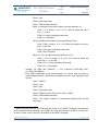
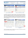
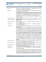
4.2.4 Filter
This section provides all the configuration options to specify the behaviour of the Kalman
Filter. In particular, the selection of measurement and the parameters to be estimated can
be chosen in this section. Figure 4-7 shows a screenshot of the FILTER section.
Figure 4-7: Filter section screenshot
•
Troposphere: Activates the estimation of the troposphere. This estimation tries to
remove the part of the wet troposphere delay not removed by the nominal modeling
(see
Software User Manual
Page 33 of 69
gAGE/UPC owns the copyright of this document which shall not be used for any purpose other than for which it is supplied and shall not be copied or given
to any person or organization without written authorization from the owner.
gAGE/UPC
gAGE
Research group of Astronomy & Geomatics
Technical University of Catalonia
http://www.gage.es
ESA GNSS Education
EDUNAV
Ref.:
EDUNAV-SUM-gAGE/UPC
Iss./Rev.:
1.7
Date:
1/07/2011
Modeling section). The estimation depends on the model chosen to compute the
mwet(elev) function (Niell mapping should be used for more realistic results).
IMPORTANT: Reliable troposphere estimation can only be obtained following
options:
Navigation Mode: PPP Template
Measurements: Pseudorange + Carrier phase
Available frequencies: Dual Frequency
Outside this specific case, the troposhere estimation should be disabled.
•
•
Available Frequencies: Select which frequencies are available.
o
Single Frequency: Use this option to force the receiver to be understood as a
single-frequency one. Discarding all the measurements in the F2. For
conditions with the rest of the values of this window, see SPP/PPP
Navigation Mode Templates.
o
Dual Frequency: Use this option to have the measurements for both
frequencies (F1 and F2) available. For conditions with the rest of the values
of this window, see SPP/PPP Navigation Mode Templates tooltips.
Receiver Kinematics: Select which is the supposed movement of the receiver.
o
Static: Select this option to do a processing supposing that the receiver is
static. This modifies the filter parameters Phi (propagation) and Q (process
noise) for the positions to: Phi = 1 and Q = 0.
o
Kinematic: Select this option to do a processing supposing that the receiver
is in movement. This modifies the filter parameters Phi (propagation) and Q
(process noise) for the positions to: Phi = 0 and Q = inf.
•
Other options: Backward filtering. This kind of processing reverses the input
observation RINEX file when it reaches the end of the file, and processes it
backwards. This is also called smoothing and it allows to have good estimation of
the parameters (such as the troposphere, and the position in a kinematic receiver) in
the beginning of the file, what would be the convergence period.
•
Measurement configuration and noise: Section to specify the input measurements
used in the filter, and its corresponding standard deviation noise (to be used for the
filter weights).
o
Selection:
Software User Manual

Pseudorange: Use only pseudorange measurements for the
processing. The ambiguity estimation in the filter will be disconnected
with this option set. For conditions with the rest of the values of this
window, see SPP/PPP Navigation Mode Templates.

Pseudorange + Carrier phase: Use both pseudorange and carrier
phase measurements for the processing. For conditions with the rest
of the values of this window, see SPP/PPP Navigation Mode
Templates.
Page 34 of 69
gAGE/UPC owns the copyright of this document which shall not be used for any purpose other than for which it is supplied and shall not be copied or given
to any person or organization without written authorization from the owner.
gAGE/UPC
gAGE
Research group of Astronomy & Geomatics
Technical University of Catalonia
http://www.gage.es

ESA GNSS Education
EDUNAV
Ref.:
EDUNAV-SUM-gAGE/UPC
Iss./Rev.:
1.7
Date:
1/07/2011
Pseudorange smoothing [epochs]: Use the Hatch filter to smooth the
pseudorange measurements with carrier phase one. This option will
reduce the noise of the measurements included in the filter. This
should only be activated when processing with pseudorange only (no
carrier phase), as the carrier phase is better included in the filter in
that other way better than using smoothing. The use of smoothing
allows to enhance the pseudorange without the cost of the increased
filter complexity for carrier phase amibiguities estimations. The Hatch
filter is defined as:
Pi,smoothed = mean(P-L)i+ Li
Being the mean() a function that computes the mean of pseudorange
and carrier phase measurements. This mean at epoch i is obtained:
mean(P-L)i = ((n-1)*mean(P-L)i-1 + (P-L)i)/n
being n the arc length at epoch i limited to a maximum value. This
limitation is to reduce the effect of the ionospheric divergence
between pseudorange and carrier phase measurements. If both
measurements do not have ionospheric divergence (i.e. Pc and Lc),
the parameter can be as high as desired.
o
Configuration.

[Grayed option]: Selected measurements for the filter.

Fixed stdDev [m]: This sets the standard deviation of the
corresponding measurement to be used as weight in the filter. The
weight is computed as:
W = 1/(stdDev)2

Elevation stdDev: This sets the standard deviation of the
corresponding measurement to be used as weight in the filter as a
function of the elevation. The standard deviation is computed as:
stdDev = a + b·e^(elev/c)
Being a, b and c the three parameters, and elev the elevation in
degrees of the satellite. The filter weight is finally computed as:
W = 1/(stdDev)2
•
Parameters:
o
Phi: Phi sets the propagation of parameters between epochs (transition state
matrix). '1' means that the value estimated in the epoch i+1 is used as apriori
value in the epoch i, '0', means that the apriori value is always '0'.
o
Q: The process noise parameter (Q) sets the stability of a parameter along
time. The process noise is included after the estimation when propagating
the parameters to the next epoch, and is an increase in the covariance of the
parameter. A process noise of '0' means that the parameter is a constant.
o
P0: The Kalman filter requieres initial values for all its parameters:
Software User Manual
Page 35 of 69
gAGE/UPC owns the copyright of this document which shall not be used for any purpose other than for which it is supplied and shall not be copied or given
to any person or organization without written authorization from the owner.
gAGE
gAGE/UPC
Research group of Astronomy & Geomatics
Technical University of Catalonia
http://www.gage.es
ESA GNSS Education
EDUNAV
Ref.:
EDUNAV-SUM-gAGE/UPC
Iss./Rev.:
1.7
Date:
1/07/2011
Position: The Apriori receiver position in the Input section is used.
Clock: A '0' value is assigned due to its high variability.
Troposphere: Due to the fact that about 90% of the troposphere is
corrected by a proper modeling, and only about a 10% has to be
estimated (and is usually around 10 cm), a '0' value is used for
apriori.
Carrier phase ambiguities: As carrier phase is prealigned with code,
the ambiguities are not far from '0', thence this value is used as
apriori.
The parameter P0 sets the initial uncertainty of these apriori values.
o
Position: This comprises the 3 parameters with the 3D position [XYZ] of the
receiver. Typical values:
Apriori value: Apriori receiver position, configured in Input section.
Phi: '1' [Static positioning], '0' [Kinematic positioning].
Process noise: '0' [Static positioning], 'inf' [Kinematic positioning].
Initial covariance: 'inf' (A smaller value for the initial covariance will
increase the convergence time, but would require a good initial
position).
o
Receiver Clock: This parameter is the receiver clock synchronism error
referring to GPS time scale. Typical values:
Apriori value: '0'.
Phi: '0'.
Process noise: 'inf'.
Initial covariance: 'inf'.
o
Troposphere: This parameter estimates part of the troposphere not taken into
account in the nominal model (see Modeling section). This 10% is mostly
associated with the wet component of the troposphere, which is due to the
water vapor of the atmosphere. The mapping mwet(elev) function described in
the Modeling section is used in the troposhere estimation. Typical values:
Apriori value: '0'.
Phi: '1'.
Process noise: '1e-4' in units of [m²/h]. Contrary to the rest of
parameters, troposphere process noise is given as increase of Q per
time unit.
Initial covariance: '0.025' (equivalent to 0.5 meters of uncertainty).
o
Phase ambiguities: Carrier phase ambiguities are the parameters which
estimates the ambiguities of the carrier phase measurements (or
combinations) used in the filter. Each epoch, there is one parameter for each
Software User Manual
Page 36 of 69
gAGE/UPC owns the copyright of this document which shall not be used for any purpose other than for which it is supplied and shall not be copied or given
to any person or organization without written authorization from the owner.
gAGE
gAGE/UPC
Research group of Astronomy & Geomatics
Technical University of Catalonia
http://www.gage.es
ESA GNSS Education
EDUNAV
Ref.:
EDUNAV-SUM-gAGE/UPC
Iss./Rev.:
1.7
Date:
1/07/2011
satellite. Additionally, when a cycle-slip is detected, the carrier phase
ambiguity is reset (by providing a new initial value and covariance).Typical
values:
Phi: '1'
Process noise: '0'.
Initial covariance: '400' (equivalent to 20 meters in relation to the
pseudorange measurement used to prealign the carrier phase).
Software User Manual
Page 37 of 69
gAGE/UPC owns the copyright of this document which shall not be used for any purpose other than for which it is supplied and shall not be copied or given
to any person or organization without written authorization from the owner.
gAGE/UPC
gAGE
Research group of Astronomy & Geomatics
Technical University of Catalonia
http://www.gage.es
ESA GNSS Education
EDUNAV
Ref.:
EDUNAV-SUM-gAGE/UPC
Iss./Rev.:
1.7
Date:
1/07/2011
4.2.5 Output
This section provides all the configuration options to select which messages are output.
Figure 4-8 shows a screenshot of the OUTPUT section.
Figure 4-8: Output section screenshot
•
Output Destination: Sets the output file where all messages will be written.
•
Messages: Individually select which messages are printed.
o
Print INFO Messages: INFO messages are shown at several points in the
program and provide information on the program configuration and problems
it may encounter.
o
Print CS (Cycle-Slip) Messages: CS messages are shown when a cycle-slip
is found by any detector. The first 5 fields are fixed, afterwards, there are
three possible blocks depending on the cycle-slip detector activated.
Field 1: 'CS'
Field 2: Year
Software User Manual
Page 38 of 69
gAGE/UPC owns the copyright of this document which shall not be used for any purpose other than for which it is supplied and shall not be copied or given
to any person or organization without written authorization from the owner.
gAGE
gAGE/UPC
Research group of Astronomy & Geomatics
Technical University of Catalonia
http://www.gage.es
ESA GNSS Education
EDUNAV
Ref.:
EDUNAV-SUM-gAGE/UPC
Iss./Rev.:
1.7
Date:
1/07/2011
Field 3: Doy
Field 4: Seconds of day
Field 5: PRN satellite identifier
Block 1: Geometric-free carrier phase cycle-slip detector (Li)
Field 1: 'Li:x', being x, 0 or 1 (0-> Li did not detect the cycleslip, 1-> Li did)
Field 2: Li value (estimated-observed)
Field 3: Li Threshold
Block 2: Melbourne-Wübbena cycle-slip detector (Bw)
Field 1: 'Bw:x', being x, 0 or 1 (0-> Bw did not detect the cycleslip, 1-> Bw did)
Field 2: Bw value (estimated-observed)
Field 3: Bw Threshold
Block 3: L1-C1 average cycle-slip detector (L1C1)
Field 1: 'L1C1:x', being x, 0 or 1 (0-> L1C1 did not detect the
cycle-slip, 1-> L1C1 did)
Field 2: L1C1 value (estimated-observed)
Field 3: L1C1 Threshold
Sample: CS 2006 200 25350.00
(3.747907 [0.900000])
o
1 Li:0 (6.266301 [0.052100]) Bw:1
Print INPUT Messages: Input data message. It is shown after an epoch is
read (and decimated). It contains the measurements for each satellite for this
epoch 3.
Field 1: 'INPUT'
Field 2: Year
Field 3: Doy
Field 4: Seconds of day
Field 5: GNSS System (GPS, GAL, GLO or GEO)
Field 6: PRN satellite identifier
Field 7: Arc length (number of undecimated epochs after the last
cycle-slip)
3
These measurements are the ones that are shown in the INPUT message. Nevertheless
all the measurements included in the RINEX are read and stored by gLAB for its later use,
in case of need, even if they are not printed in the INPUT message.
Software User Manual
Page 39 of 69
gAGE/UPC owns the copyright of this document which shall not be used for any purpose other than for which it is supplied and shall not be copied or given
to any person or organization without written authorization from the owner.
gAGE
gAGE/UPC
Research group of Astronomy & Geomatics
Technical University of Catalonia
http://www.gage.es
ESA GNSS Education
EDUNAV
Ref.:
EDUNAV-SUM-gAGE/UPC
Iss./Rev.:
1.7
Date:
1/07/2011
For GPS:
Field 8: C1 [C1C]
Field 9: P1 [C1P]
Field 10: P2 [C2P]
Field 11: L1 [L1P] (prealigned, in meters)
Field 12: L2 [L2P] (prealigned, in meters)
For Galileo (GAL):
Field 8: C1A
Field 9: C1B
Field 10: C1C
Field 11: C7Q
Field 12: C8Q
Field 13: L1A (prealigned, in meters)
Field 14: L1B (prealigned, in meters)
Field 15: L1C (prealigned, in meters)
Field 16: L7Q (prealigned, in meters)
Field 17: L8Q (prealigned, in meters)
For GLONASS (GLO):
Field 8: C1 [C1C]
Field 9: C2 [C2C]
Field 10: L1 [L1P] (prealigned, in meters)
Field 11: L2 [L2P] (prealigned, in meters)
For GEO:
Field 8: C1 [C1C]
Sample: INPUT 2006 200 0.00 GPS 19 1 23119003.9020 23119002.6110
23119004.0750 23119002.7507 23119004.0925
o
Print MEAS Messages: It provides the MEASurement values. It is shown after
an epoch is read (and decimated). It contains the measurements for each
satellite for this epoch.
Field 1: MEAS
Field 2: Year
Field 3: Doy
Field 4: Seconds of day
Software User Manual
Page 40 of 69
gAGE/UPC owns the copyright of this document which shall not be used for any purpose other than for which it is supplied and shall not be copied or given
to any person or organization without written authorization from the owner.
gAGE
gAGE/UPC
Research group of Astronomy & Geomatics
Technical University of Catalonia
http://www.gage.es
ESA GNSS Education
EDUNAV
Ref.:
EDUNAV-SUM-gAGE/UPC
Iss./Rev.:
1.7
Date:
1/07/2011
Field 5: GNSS System (GPS, GAL, GLO or GEO)
Field 6: PRN satellite identifier
Field 7: Elevation of the satellite [degrees]
Field 8: Azimuth of the satellite [degrees]
Field 9: Number of Measurement(s)
Field 10: Measurement identifier (as string)
Field 11: Measurement(s) value [m]
Sample: MEAS 2010 081 300.00 GPS
C1C:L1C:C1P:L1P:C2P:L2P
20228715.3270
20228715.2722 20228714.8230 20228714.7005
o
30 30.00
0.0000
240.00 6
0.0000
Print MODEL Messages: Model break down message. It is shown when a
model can be fully computed for each measurement.
Field 1: 'MODEL'
Field 2: Year
Field 3: Doy
Field 4: Seconds of day
Field 5: GNSS System (GPS, GAL, GLO or GEO)
Field 6: PRN satellite identifier
Field 7: Measurement identifier (as string)
Field 8: Signal flight time [sec]
Field 9: Measured value [m]
Field 10: Full model value [m]
Field 11: Satellite X position [m]
Field 12: Satellite Y position [m]
Field 13: Satellite Z position [m]
Field 14: Satellite X velocity [m]
Field 15: Satellite Y velocity [m]
Field 16: Satellite Z velocity [m]
Field 17: Satellite-receiver geometric distance [m]
Field 18: Satellite clock correction [m]
Field 19: Satellite phase center projection [m]
Field 20: Receiver phase center projection [m]
Software User Manual
Page 41 of 69
gAGE/UPC owns the copyright of this document which shall not be used for any purpose other than for which it is supplied and shall not be copied or given
to any person or organization without written authorization from the owner.
gAGE
gAGE/UPC
Research group of Astronomy & Geomatics
Technical University of Catalonia
http://www.gage.es
ESA GNSS Education
EDUNAV
Ref.:
EDUNAV-SUM-gAGE/UPC
Iss./Rev.:
1.7
Date:
1/07/2011
Field 21: Receiver Antenna Reference Point (ARP) projection [m]
Field 22: Relativistic clock correction [m]
Field 23: Wind-up correction [m] (for carrier phase measurements)
Field 24: Troposphere nominal correction [m]
Field 25: Ionosphere correction [m]
Field 26: Relativistic path range correction [m]
Field 27: Total Group Delay (TGD) correction [m]
Field 28: Solid tides correction [m]
Field 29: Elevation of the satellite [degrees]
Field 30: Azimuth of the satellite [degrees]
Sample: MODEL 2006 200 0.00 GPS 19 L1P 0.07712 23119002.7507
23119008.7502 8811456.7780 -21033910.1687 13675922.8867 1828.7339
2353.7679 2467.3576 23119457.7539 -456.317873 0.000000 -0.049360
0.000000 2.323328 0.106706 4.854110 -0.000000 0.015435 0.000000
0.063943 9.16487738221 -79.27496674531
The satellite coordinates (fields 11-16) are given in the reception epoch if the
model of the signal transmission time is enabled (if it is disabled, they are
given in the transmission time). The coordinates are relative of the antenna
phase center or satellite mass center, depending on the option chosen in the
Input section:
•
Broadcast: Antenna Phase Center.
•
Precise: Satellite Mass Center.
Field 9 is the direct measurement (as in the RINEX file), but scaled to meters
for carrier phase measurements. Field 10 is the model computed for this
measurement. Field 10 is the direct sum of fields 17 to 28.
o
Print EPOCHSAT Messages: Message with the satellites used to compute
the solution. It is shown when the filter is run, and is given for each
measurement
Field 1: 'EPOCHSAT'
Field 2: Year
Field 3: Doy
Field 4: Seconds of day
Field 5: Measurement identifier (as string)
Field 6: Number of satellites in view
Field 7-: Each following column is the identifier of a satellite
Software User Manual
Page 42 of 69
gAGE/UPC owns the copyright of this document which shall not be used for any purpose other than for which it is supplied and shall not be copied or given
to any person or organization without written authorization from the owner.
gAGE
gAGE/UPC
Research group of Astronomy & Geomatics
Technical University of Catalonia
http://www.gage.es
ESA GNSS Education
EDUNAV
Ref.:
EDUNAV-SUM-gAGE/UPC
Iss./Rev.:
1.7
Date:
1/07/2011
Sample: EPOCHSAT 2006 200 300.00 PC 7 15 3 19 16 18 21 22
o
Print SATSEL Messages: Message with debug information of the reason why
a satellite has been discarded (or selected) for processing.
Sample: SATSEL 7 discarded: Elevation too low ( 3.04 )
o
Print PREFIT Messages: Prefilter values message. It provides the
measurement-model values. It is shown in each filter execution.
Field 1: 'PREFIT' (if the satellite is used in the computation) or
'PREFIT*' (if it is not)
Field 2: Year
Field 3: Doy
Field 4: Seconds of day
Field 5: GNSS System (GPS, GAL, GLO or GEO)
Field 6: PRN satellite identifier
Field 7: Measurement identifier (as string)
Field 8: Measurement-model value (prefit) [m]
Field 9: Measurement value [m]
Field 10: Model value [m]
Field 11: Elevation of the satellite [degrees]
Field 12: Azimuth of the satellite [degrees]
Sample: PREFIT 2006 200 300.00 GPS 19 LC -7.3029 22982271.7155
22982279.0184 28.28 -77.91
In general Field 8 = Field 9 - Field 10, but this is no longer true when using
smoothing, as the Field 9 is the raw measurement without smoothing, but the
Field 8 computation takes smoothing into account.
o
Print POSTFIT Messages: Postfilter values message. It provides the
corrected prefits with the filter estimation. It is shown in each filter execution.
Field 1: 'POSTFIT'
Field 2: Year
Field 3: Doy
Field 4: Seconds of day
Field 5: GNSS System (GPS, GAL, GLO or GEO)
Field 6: PRN satellite identifier
Field 7: Measurement identifier (as string)
Field 8: Measurement-corrected model value (postfit) [m]
Field 9: Measurement value [m]
Software User Manual
Page 43 of 69
gAGE/UPC owns the copyright of this document which shall not be used for any purpose other than for which it is supplied and shall not be copied or given
to any person or organization without written authorization from the owner.
gAGE
gAGE/UPC
Research group of Astronomy & Geomatics
Technical University of Catalonia
http://www.gage.es
ESA GNSS Education
EDUNAV
Ref.:
EDUNAV-SUM-gAGE/UPC
Iss./Rev.:
1.7
Date:
1/07/2011
Field 10: Corrected model value with the filter estimations[m]
Field 11: Elevation of the satellite [degrees]
Field 12: Azimuth of the satellite [degrees]
Field 13: Only given for carrier phase measurements. It is the
estimated carrier phase ambiguity. [m]
Sample: POSTFIT 2006 200 300.00 GPS 19 PC -0.0160 22982271.6557
22982270.5509 28.28 -77.91
As with PREFIT messages, Field 8 is not necessary Field 9 - Field 10 when
using smoothing.
o
Print FILTER Messages: Filter solution message. This message provides
direct information on the filter estimates. It is shown in each filter execution.
Field 1: 'FILTER'
Field 2: Year
Field 3: Doy
Field 4: Seconds of day
Field 5-: Filter estimates. The order is: 3D estimated position, clock,
troposphere and ambiguities. The number of fields is variable in this
message. With a full filter (troposphere and ambiguities estimation),
the fileds are as follows:
Field 5: Receiver X position [m]
Field 6: Receiver Y position [m]
Field 7: Receiver Z position [m]
Field 8: Receiver clock [m]
Field 9: Troposphere [m]
Field 10: Carrier phase ambiguities [m]
Sample: FILTER 2006 200 300.00 4849202.0700 -360328.8991
4114913.3520 -8.4316 -0.0010 -0.0001 0.9389 -0.8663 1.1051 0.2317
0.0707 0.0001 0.5066 0.2393
o
Print OUTPUT Messages: Receiver solution message. This message
provides the estimated receiver position. It is shown in each filter execution.
Field 1: 'OUTPUT'
Field 2: Year
Field 3: Doy
Field 4: Seconds of day
Field 5: Square root of the sum of the covariance matrix. This is a
measure of the convergence of the filter
Software User Manual
Page 44 of 69
gAGE/UPC owns the copyright of this document which shall not be used for any purpose other than for which it is supplied and shall not be copied or given
to any person or organization without written authorization from the owner.
gAGE
gAGE/UPC
Research group of Astronomy & Geomatics
Technical University of Catalonia
http://www.gage.es
ESA GNSS Education
EDUNAV
Ref.:
EDUNAV-SUM-gAGE/UPC
Iss./Rev.:
1.7
Date:
1/07/2011
Field 6: Receiver X position [m]
Field 7: Receiver Y position [m]
Field 8: Receiver Z position [m]
Field 9: Receiver X position - Nominal apriori X position [m]
Field 10: Receiver Y position - Nominal apriori Y position [m]
Field 11: Receiver Z position - Nominal apriori Z position [m]
Field 12: Receiver X formal error [m]
Field 13: Receiver Y formal error [m]
Field 14: Receiver Z formal error [m]
Field 15: Receiver latitude [degrees]
Field 16: Receiver longitude [degrees]
Field 17: Receiver height [m]
Field 18: Receiver North difference in relation to nominal apriori
position [m]
Field 19: Receiver East difference in relation to nominal apriori
position [m]
Field 20: Receiver Up difference in relation to nominal apriori
position [m]
Field 21: Receiver formal error in North direction [m]
Field 22: Receiver formal error in East direction [m]
Field 23: Receiver formal error in Up direction [m]
Field 24: Horizontal Dilution of Precision (HDOP)
Field 25: Vertical Dilution of Precision (VDOP)
Field 26: Zenith Tropospheric Delay (including nominal value) [m]
Field 27: Zenith Tropospheric Delay (excluding nominal value) [m]
Field 28: Zenith Tropospheric Delay formal error [m]
Sample: OUTPUT 2006 200 300.00 2.6219 4849202.0700 -360328.8991
4114913.3520 -0.3037 0.0397 0.1401 1.9353 0.6998 1.6246 40.429164806 4.249658495 829.311998170 0.3057 0.0171 -0.1403 1.1365 0.6772 2.2637
0.9572 1.8306 2.1982 0.0097 0.4995
Providing a nominal a priori position is option for the processing, but if it is
given, fields 9, 10, 11, 18, 19 and 20 will be given to this a priori position. See
the option A priori Receiver Position in the INPUT section.
Software User Manual
Page 45 of 69
gAGE/UPC owns the copyright of this document which shall not be used for any purpose other than for which it is supplied and shall not be copied or given
to any person or organization without written authorization from the owner.
gAGE/UPC
gAGE
Research group of Astronomy & Geomatics
Technical University of Catalonia
http://www.gage.es
ESA GNSS Education
EDUNAV
Ref.:
EDUNAV-SUM-gAGE/UPC
Iss./Rev.:
1.7
Date:
1/07/2011
4.3 ANALYSIS (DAT INTERFACE)
The analysis tab allows configuring all the visualization options for the DAT. Figure 4-9
shows a screenshot of the Analysis tab.
Figure 4-9: Analysis tab screenshot
•
Templates: The templates are a set of preconfigured plotting options for the Graphic
Details section. Clicking on any button will load the options in that section, allowing
modifying or plotting them directly.
o
NEU position error: The NEU position error template sets the options to print
the three components (North, East and Up) of the error of the receiver
positioning obtained by the filter. This error is computed by the difference
between the direct filter estimation and the Apriori Receiver Position in the
Input section of Calculus. Thence to obtain a reliable error estimation, this
apriori position should be precise.
If you do not have any precise position of the receiver, you can obtain it by
doing a PPP processing (SP3/Static/Dual frequency/Pseudorange+Carrier
phase). The XYZ position (fields 6 to 8 of OUTPUT message) of the last
Software User Manual
Page 46 of 69
gAGE/UPC owns the copyright of this document which shall not be used for any purpose other than for which it is supplied and shall not be copied or given
to any person or organization without written authorization from the owner.
gAGE/UPC
gAGE
Research group of Astronomy & Geomatics
Technical University of Catalonia
http://www.gage.es
ESA GNSS Education
EDUNAV
Ref.:
EDUNAV-SUM-gAGE/UPC
Iss./Rev.:
1.7
Date:
1/07/2011
epoch should have an accuracy in the order of the centimeter, and can be
used as a good reference position.
•
o
North-East dispersion: The North-East dispersion template sets the options
to print the North vs East position error components. This provides an insight
of the horizontal dispersion and bias of the errors.
o
Model components: The Model components template sets the options to print
a component of the model as a function of time. By default, it selects the
Relativity effect, but it can easily be chosen which model to print, by selecting
it in the Y Column option.
o
Ionospheric combinations: The Ionospheric combinations template sets the
options to print the two ionospheric (geometric-free) combinations: PI (P2-P1)
[pseudorange] and LI (L1-L2) [carrier phase].
o
Zenith Tropospheric Delay: The Zenith Tropospheric Delay template sets the
options to print the tropospheric estimations as a function of time. It includes
the nominal part corrected in the modelling and the estimated part computed
in the filter.
o
Postfit residuals: The Postfit residuals template sets the options to print the
filter residuals (postfits) as a function of the satellite elevation. It prints both
pseudorange and carrier phase postfits. This plot allows observing the
dependence of residuals from elevation. In general, carrier phase residuals
will be quite independent from elevation, and pseudorange residuals can
have a large dependence on elevation.
o
Satellite skyplot: The Satellite skyplot template sets the options to print the
elevation/azimuth of the satellites in a skyplot, being the center of the plot the
zenith of the satellite, and the extremes, the lower elevations. This is a
special plot which makes use of sin and cos in the X column and Y column to
obtain a polar plot.
o
Carrier phase ambiguities: The Carrier phase ambiguities template sets the
options to print the estimation of carrier phase measurements in the filter.
This is only possible in a processing with the Pseudorange + carrier phase
measurements (in the Filter section).
Global Graphic Parameters: Specify the different options of the graphic.
o
Title: Sets the title of the graphic.
o
X-label: Sets the X label of the graphic.
o
Y-label: Sets the Y label of the graphic.
o
Clear: Clear all the options in the Graphic Details section.
o
Automatic Plot Limits: The limits of the graphic axis can be automatically or
user set:
Software User Manual

Xmin & Xmax

Ymin & Ymax
Page 47 of 69
gAGE/UPC owns the copyright of this document which shall not be used for any purpose other than for which it is supplied and shall not be copied or given
to any person or organization without written authorization from the owner.
gAGE/UPC
gAGE
Research group of Astronomy & Geomatics
Technical University of Catalonia
http://www.gage.es
o
ESA GNSS Education
EDUNAV
Ref.:
EDUNAV-SUM-gAGE/UPC
Iss./Rev.:
1.7
Date:
1/07/2011
Individual Plot(s) Configuration: Options for the different plots that can
contain a graphic (up to four plots).

Plot 1/2/3/4: Selector for each plot. The options below this one are
plot-dependent.

Source File: Selects the source input file for the plot.

Lines/Dot list: Allows changing the style of the plot, using Lines or
Dots among many plot marker styles.

Color Selection: Allows changing the color of the plot.

Condition: The condition is a way to insert one or more conditions in
order to select which lines of the source file will be used in the
plotting. This has a space to write the required conditions and two
comboboxes, which automatically sets the condition text. The text is
the only that matters and the combo boxes only configure the text.
To specify a column, it should be done as '$x' being x the number of
the column. For example if you would like to specify the condition that
the sixth column must be greater or equal than 10, you should do it
as: ($6>=10)
You can specify a set of conditions by using AND [&] and OR [|]
operators, such as: ($6>=10) &($6<=20)|($8==2)
You can specify that a column matches a specific string by
surrounding the string by \", such as: ($1==\"OUTPUT\")
You can specify mathematical operations and constants, as: math.pi,
math.e,
math.sin()
and
math.cos(),
as
example:
($1==\"POSTFIT\")&(math.cos($11+5)>0.707)
You can specify a specific character inside a column, by using $x[y],
being x the column and y the character position beginning by 0, such
as: ($1==\"POSTFIT\")&($7[0]==\"P\") [First character of seventh
column is 'P']
You can also operate between columns, such as: (($9-$11)<2)
•

X Column: This allows specifying the column for the x values for the
selected plot. The combo box will be updated by the First condition,
but the text part is the one that matters. As in the conditions, you can
specify several things. In general if it is required to plot a column it
can be done by putting its column position, such as: 4. It can also be
used the $4 to plot the forth column. As before, operations between
scalars and columns can be done (and even use functions), such as:
($9*2-$11*3-1.5).

Y Column: This allows specifying the column for the y values for the
selected plot. The format is the same as in X Column.

Label: Sets the label for the selected plot.
Plot button: This button executes the plotting tool of gLAB with the specified options.
Software User Manual
Page 48 of 69
gAGE/UPC owns the copyright of this document which shall not be used for any purpose other than for which it is supplied and shall not be copied or given
to any person or organization without written authorization from the owner.
gAGE/UPC
gAGE
Research group of Astronomy & Geomatics
Technical University of Catalonia
http://www.gage.es
ESA GNSS Education
EDUNAV
Ref.:
EDUNAV-SUM-gAGE/UPC
Iss./Rev.:
1.7
Date:
1/07/2011
4.4 GUI LIMITATIONS
For an increased easiness in use, the GUI does not include all the different options that the
DPC is able to cope. In order to use these GUI-excluded features, the command-line DPC
program should be used instead (see section 5 GLAB Data Processing Core (DPC)). In
particular, the following cases are not covered by the GUI:
•
The DPC is able to compare two different sets of orbit and clocks.
•
Besides from ANTEX, the DPC can also read the GPSConstellationStatus.txt file
(which can be found in [RD-12]), compiled and updated by Richard B. Langley. This
file provides a dictionary between satellite PRN and SVN, and its corresponding
GPS Block. This allows correcting the phase centers of the satellites.
•
The GUI pseudorange smoothing configuration is only based on the smoothing
window to use. DPC also allows to specify which measurement will smooth which
(by means of the ‘-pre:smoothMeas’ option).
•
The GUI Available Frequencies option of Filter section, can only take two different
values: Single or Dual Frequency. With the DPC it is possible the specify availability
of each frequency (for example setting as available F1 and F5 of GPS) by means of
the ‘-pre:availf’ option.
Software User Manual
Page 49 of 69
gAGE/UPC owns the copyright of this document which shall not be used for any purpose other than for which it is supplied and shall not be copied or given
to any person or organization without written authorization from the owner.
gAGE
gAGE/UPC
Research group of Astronomy & Geomatics
Technical University of Catalonia
http://www.gage.es
ESA GNSS Education
EDUNAV
Ref.:
EDUNAV-SUM-gAGE/UPC
Iss./Rev.:
1.7
Date:
1/07/2011
4.5 PROCESSING EXAMPLE
The next example gives an overview of a simple processing using gLAB, following all the
steps from selecting input files to generating plots to analyse the data. The sample will
cover a precise static positioning to obtain the precise coordinates of a station.
After opening the gLAB, the splash screen is shown (Figure 4-10). Clicking the Input button
will open the Input section (Figure 4-11). Clicking the PPP Template button will preconfigure
the GUI for a basic PPP. Clicking the Examine button for the RINEX Observation File will
allow selecting which RINEX observation file will be used.
Figure 4-10: GUI Splash screen
Figure 4-11: Input section
A file dialog will open (Figure 4-12), in order to go to the test directory (where all sample
data files are found), the “Go Back one directory” button should be pressed, and afterwards
doubleclick in “test” (Figure 4-13).
Figure 4-12: File Open dialog (1/3)
Software User Manual
Figure 4-13: File Open dialog (2/3)
Page 50 of 69
gAGE/UPC owns the copyright of this document which shall not be used for any purpose other than for which it is supplied and shall not be copied or given
to any person or organization without written authorization from the owner.
gAGE/UPC
gAGE
Research group of Astronomy & Geomatics
Technical University of Catalonia
http://www.gage.es
ESA GNSS Education
EDUNAV
Ref.:
EDUNAV-SUM-gAGE/UPC
Iss./Rev.:
1.7
Date:
1/07/2011
The directory where all the data is stored will be the one active (Figure 4-14). Double
clicking on “madr2000.06o” will select this file and include it in the Input section (Figure
4-15). In order to include the rest of the required files, it should be clicked the Examine of
ANTEX File (selecting the file “igs_pre1400.atx”), and the Examine of SP3 File (selecting
the file “igs13843.sp3”).
Figure 4-14: File Open dialog (3/3)
Figure 4-15: Updated Input section
Once input files are selected (Figure 4-16), Filter section button should be clicked in order to
configure all the filter parameters. Once in this screen (Figure 4-17), the following
parameters should be used (if not already checked):
•
Navigation mode: PPP Template
•
Estimate troposphere: Yes
•
Available frequencies: Dual frequency
•
Receiver Kinematics: Static
•
Measurement selection: Pseudorange + Carrier phase
All these parameters are the default ones, so no special change should be done if the
program has just started. After being sure all parameters are properly selected, the output
file should be selected by clicking in the Output section.
Software User Manual
Page 51 of 69
gAGE/UPC owns the copyright of this document which shall not be used for any purpose other than for which it is supplied and shall not be copied or given
to any person or organization without written authorization from the owner.
gAGE
gAGE/UPC
Research group of Astronomy & Geomatics
Technical University of Catalonia
http://www.gage.es
ESA GNSS Education
EDUNAV
Figure 4-16: All input files are selected
Ref.:
EDUNAV-SUM-gAGE/UPC
Iss./Rev.:
1.7
Date:
1/07/2011
Figure 4-17: Filter section
In the Output section (Figure 4-18), the Examine button can be clicked to select the output
file, Figure 4-19 shows the File Open dialog that will open. Writing “gLAB.out” and clicking
enter will select this file name as output for the processing.
Figure 4-18: Output section
Figure 4-19: File open dialog for selecting the
output file
After selecting the output (Figure 4-20) the RUN button will execute gLAB DPC with the
selected options. While the DPC is running, the RUN button will be grey in order to avoid
multiple clicks. After some seconds, the processing will end. To analyse the results click on
the Analysis tab (Figure 4-21).
Software User Manual
Page 52 of 69
gAGE/UPC owns the copyright of this document which shall not be used for any purpose other than for which it is supplied and shall not be copied or given
to any person or organization without written authorization from the owner.
gAGE
gAGE/UPC
Research group of Astronomy & Geomatics
Technical University of Catalonia
http://www.gage.es
ESA GNSS Education
EDUNAV
Figure 4-20: Output selected
Ref.:
EDUNAV-SUM-gAGE/UPC
Iss./Rev.:
1.7
Date:
1/07/2011
Figure 4-21: DPC has been executed
As explained in section 4.3 the Analysis tab (Figure 4-22) contains several templates in
order to ease the generation of plots, in this sense, to plot the evolution of the receiver
position in North/East/Up components the button Receiver NEU position error should be
clicked. Figure 4-23 shows the configuration of the Graphic Details with this template. The
Source File is the file selected in the Output section of the Calculus tab. Clicking the Plot
button will generate this plot. While the program is processing the source file, the Plot
button will be kept grey.
Figure 4-22: Analysis tab
Figure 4-23: Receiver NEU position error
configuration
When the processing is finished, a window will open (Figure 4-24) showing the generated
plot, and the Plot button will be again available.
Software User Manual
Page 53 of 69
gAGE/UPC owns the copyright of this document which shall not be used for any purpose other than for which it is supplied and shall not be copied or given
to any person or organization without written authorization from the owner.
gAGE
gAGE/UPC
Research group of Astronomy & Geomatics
Technical University of Catalonia
http://www.gage.es
ESA GNSS Education
EDUNAV
Figure 4-24: Plot sample
Ref.:
EDUNAV-SUM-gAGE/UPC
Iss./Rev.:
1.7
Date:
1/07/2011
Figure 4-25: Plot sample (zoom)
The plotting utility allows zooming, moving and saving the current plot as a picture. All these
functions can be accessed through the top toolbar. Figure 4-25 shows a zoom of the y axis.
As would be expected for a PPP processing, the final position error is in the order of 1 cm.
Software User Manual
Page 54 of 69
gAGE/UPC owns the copyright of this document which shall not be used for any purpose other than for which it is supplied and shall not be copied or given
to any person or organization without written authorization from the owner.
gAGE/UPC
gAGE
Research group of Astronomy & Geomatics
Technical University of Catalonia
http://www.gage.es
ESA GNSS Education
EDUNAV
Ref.:
EDUNAV-SUM-gAGE/UPC
Iss./Rev.:
1.7
Date:
1/07/2011
5 gLAB DATA PROCESSING CORE (DPC)
The DPC is the processing tool of gLAB, it has been programmed in C with special care for
the following objectives:
•
Easy to use for an advanced user.
•
Modularized, in order to incorporate future updates.
•
Optimized for CPU and memory usage.
The options of the DPC are basically the same as the options of the GUI, with the
exceptions taken in consideration in section 4.4 GUI Limitations. The DPC can be executed
with the argument ‘-help’, which will provide detailed information of the different arguments
that can be used.
The following lines are an extract of the ‘-help’ inline information:
Options:
-help
-examples
-config
-messages
INPUT OPTIONS
-input:cfg <file>
-input:obs <file>
-input:nav <file>
-input:sp3 <file>
-input:orb <file>
-input:clk <file>
-input:con <file>
-input:ant <file>
-input:klb <file>
-input:con <file>
-input:ant <file>
-input:klb <file>
-input:dcb <file>
-input:rec <file>
-input:snx <file>
Software User Manual
Shows this help
Shows some examples to call the program
Shows some info on the configuration file
Shows the fields of each output message (see below, 'VERBOSE
OPTIONS')
Sets the input configuration file
Sets the input RINEX observation file
Sets the input RINEX navigation message file (only for
standalone)
Sets the input SP3 orbits and clocks file (only for PPP)
Sets the input SP3 orbits (only for PPP)
Sets the input clock file (only for PPP)
Sets
the
input
constellation
status
file
(default
GPSConstellationStatus.txt)
Sets the input ANTEX satellite/receiver antenna data file
Sets the input RINEX navigation file for Klobuchar corrections, if
this parameter is avoided, it is used the -input:nav file
Sets
the
input
constellation
status
file
(default
GPSConstellationStatus.txt)
Sets the input ANTEX satellite/receiver antenna data file
Sets the input RINEX navigation file for Klobuchar corrections, if
this parameter is avoided, it is used the -input:nav file
Sets the input DCB source as a .DCB file or a RINEX navigation
file.
Sets the input GPS Receiver Type file.
Sets the input SINEX file for receiver position.
Page 55 of 69
gAGE/UPC owns the copyright of this document which shall not be used for any purpose other than for which it is supplied and shall not be copied or given
to any person or organization without written authorization from the owner.
gAGE
gAGE/UPC
Research group of Astronomy & Geomatics
Technical University of Catalonia
http://www.gage.es
ESA GNSS Education
EDUNAV
Ref.:
EDUNAV-SUM-gAGE/UPC
Iss./Rev.:
1.7
Date:
1/07/2011
PREPROCESSING OPTIONS
-pre:dec #
# = number
Decimate input data by # seconds
In product comparison mode (see below, in 'WORK MODES'), it
sets the time step of the comparisons
-pre:sat g#
Exclude satellite from processing
g = character determining GNSS system (G->GPS)
# = PRN number
-pre:elevation <val> Elevation mask. Satellites below this threshold will be discarded
(in degrees) [default 0]
-pre:eclipse <val>
Discard satellites under Earth eclipse [default: enabled for PPP,
disabled for SPS]
-pre:availf g#
Mark frequencies available [default all]
g = character determining GNSS system (G->GPS)
# = frequencies available
Sample: '-pre:availf G12' Frequencies 1 and 2 of GPS available
'-pre:availf G1' Frequency 1 of GPS available, 2 unavailable
-pre:smooth <val>
Number of epochs of smoothing [default 0, which means disabled]
-pre:smoothMeas <n> <meas>
Smooth measurement in filter <n> with
measurement type <meas>
In general, <n> is a pseudorange and <meas> a carrier phase,
see option '-filter:select' for more information in the selection of
measurements to be used in the filter
Sample: '-pre:smoothMeas 1 LC'
-pre:setrecpos <val> <val> = RINEX
Set the receiver apriori position as the one
specified in the RINEX observation file [default]
<val> = SINEX
Set the receiver a priori position to be read
from a SINEX file (to be specified by the '-input:snx' parameter)
<val> = calculate
The ceiver apriori position will be calculated
by the program. This is especially useful when processing moving
receivers (trajectories) or when the approximate receiver position
is not known. With this option activated, the differential fields of
the OUTPUT message will be zero.
<val> = <x> <y> <z>
Specify the receiver apriori position in
meters
Sample:
'-pre:recpossrc
4789032.7143
176594.9690
4195013.2268'
-pre:setrectype <val> <val> = gpsrt Set the receiver type as the one specified in the
GPS_Receiver_Types file (provided by '-input:rec') [default if 'input:rec' provided]
-pre:prealign <val>
Software User Manual
<val> = 0
Set the receiver type as 'Unknown' [default]
<val> = 1
Set the receiver type as 'Cross-correlated’. In this
mode, P2 will be corrected with the DCB of P1-C1
<val> = 3
Set
the
receiver
type
as
'Consistent
measurements'.
Prealign carrier phase measurements with its corresponding
pseudorange [default on]\n");
Page 56 of 69
gAGE/UPC owns the copyright of this document which shall not be used for any purpose other than for which it is supplied and shall not be copied or given
to any person or organization without written authorization from the owner.
gAGE
gAGE/UPC
Research group of Astronomy & Geomatics
Technical University of Catalonia
http://www.gage.es
-pre:cs:li
--pre:cs:li
-pre:cs:li:min <val>
-pre:cs:li:max <val>
-pre:cs:li:t0 <val>
-pre:cs:bw
--pre:cs:bw
-pre:cs:min <val>
-pre:cs:max <val>
-pre:cs:slope <val>
-pre:cs:l1c1
--pre:cs:l1c1
Software User Manual
ESA GNSS Education
EDUNAV
Ref.:
EDUNAV-SUM-gAGE/UPC
Iss./Rev.:
1.7
Date:
1/07/2011
Use the carrier phase geometric-free combination (Li) for cycleslip detection (2 frequencies) [default]
Do not use carrier phase geometric-free combination (Li) for cycleslip detection (2 frequencies).
Li combination is a slow varying function which only has ambiguity
and ionosphere. Each epoch and satellite an expected Li value is
computed and compared against the measured one, if this
difference is above a certain threshold, a cycle-slip is marked.
This threshold is (max - (max-min)*exp(-dt/T0)), being dt the time
between epochs
Minimum threshold between estimated and measured Li values
[default 0.034]
Maximum threshold between estimated and measured Li values
[default 0.08]
Time constant to set the threshold between maximum and
minimum [default 60]
Use Melbourne-Wübbena (BW) for cycle-slip detection (2
frequencies) [default]
Do not use Melbourne-Wübbena (BW) for cycle-slip detection (2
frequencies)
BW combination is a mixed combination between carrier phase
and pseudoranges. This combination is free of ionosphere and
geometry, thence constant, but it is affected by the receiver noise
and multipath (due to the pseudorange measurements used). If
this noise is low enough, it is straight forward to detect cycle-slips,
but in noisy environments BW is not able to detect cycle-slips.
The algorithm using BW computes the mean and the standard
deviation of the last epochs in order to obtain an estimated value
and the noise level of the combination. The estimated value is
compared against the measured value, and the noise level is
used for the threshold of this difference. Difference must be lower
than standardDeviation multiplied by a number (slope). This
threshold has minimum (min) and maximum (max) saturation
values.
Minimum threshold between estimated and measured BW values
in relation to its standard deviation [default 0.9]
Maximum threshold between estimated and measured BW values
in relation to its standard deviation [default 18]
Relation between estimated and measured BW values in relation
to its standard deviation [default 9]
Use the L1-C1 combination for cycle-slip detection (1 frequency)
Do not use the L1-C1 combination for cycle-slip detection (1
frequency) [default]
The L1-C1 averages the difference between carrier phase and
pseudorange measurements in F1 for several epochs. This cycleslip detection method is very useful for single-frequency receivers,
as it only requires measurements from one frequency. As a
counterpart, the ionospheric term is different for C1 and L1
Page 57 of 69
gAGE/UPC owns the copyright of this document which shall not be used for any purpose other than for which it is supplied and shall not be copied or given
to any person or organization without written authorization from the owner.
gAGE
gAGE/UPC
Research group of Astronomy & Geomatics
Technical University of Catalonia
http://www.gage.es
ESA GNSS Education
EDUNAV
Ref.:
EDUNAV-SUM-gAGE/UPC
Iss./Rev.:
1.7
Date:
1/07/2011
thence, this combination will tend to diverge. It becomes
necessary to set a smoothing window to limit this divergence (pre:cs:l1c1:window). This makes that this method becomes a bit
limited with data rates too low. Ideally this method should be used
with rates of 1Hz or higher
-pre:cs:l1c1:slope <val>
Relation between estimated and measured L1C1 values in relation to its standard deviation [default 5]
-pre:cs:l1c1:window <val>
Number of epochs to limit the L1-C1
ionosphere divergence [default 100]
-pre:cs:l1c1:max <val>
Maximum standard deviation for the threshold
calculation in the L1-C1 [default 15] (m)
MODELING OPTIONS (use -model:... to activate, --model:... to deactivate)
-model:iono <val>
<val> = no
Do not correct ionosphere [default in PPP]
(equivalent to '--model:iono')
<val> = Klobuchar Correct measurements with klobuchar model
[default in standalone]
-model:trop:nominal <val> <val> = Simple
Compute a simple tropospheric nominal
depending on receiver's height over the sea level. [default in PPP]
<val> = UNB3
Troposphere nominals are calculated
from the receiver’s height and estimates of five meteorological
parameters: pressure, temperature, water vapour pressure,
temperature lapse rate and water vapour lapse rate. It is adopted
by SBAS systems (AD-07). [default in SPP]
-model:trop:mapping <val> <val> = Simple
Compute the mapping as the obliquity
factor described in Black and Eisner, 1984. This mapping only
depends on satellite elevation and it is common for wet and dry
components. [default in SPP].
<val> = Niell
Compute the mapping described in
A.E. Niell, 1996. This mapping considers different obliquity factors
for the wet and dry components [default in PPP].
-model:satclocks
Correct the measurements with the satellite clock error estimations
[default on]
-model:relclock
Correct the measurements with the relativistic clock model [default
on]
-model:satmovinflight Consider satellite movement during signal flight time [default on]
-model:earthrotinflight Consider Earth rotation during signal flight time [default on]
-model:satphasecenter Correct satellite phase center to mass center corrections [default
on]
-model:recphasecenter <val> <val> = no
Do not correct antenna receiver phase
center [default]
<val> = ANTEX
Use the ANTEX file to correct the
antenna phase center
<val> = <nfreq> <dN> <dE> <dU>
Software User Manual
Page 58 of 69
gAGE/UPC owns the copyright of this document which shall not be used for any purpose other than for which it is supplied and shall not be copied or given
to any person or organization without written authorization from the owner.
gAGE
gAGE/UPC
Research group of Astronomy & Geomatics
Technical University of Catalonia
http://www.gage.es
ESA GNSS Education
EDUNAV
Ref.:
EDUNAV-SUM-gAGE/UPC
Iss./Rev.:
1.7
Date:
1/07/2011
Set dN, dE, dU as the antenna phase
center for the frequency <nfreq>
<nfreq> = Frequency number (typical for GPS, 1 and
2)
-model:radomestrict
-model:arp <val>
-model:tgd <val>
<dN> = North correction [in meters]
<dE> = East correction [in meters]
<dU> = Up correction [in meters]
Sample:
'-model:recphasecenter
1
0
0
0.11
model:recphasecenter 2 0 0 0.128'
Typical AOAD/M_T antenna phase center correction, 11 cm and
12.8 cm in the Up component for frequencies 1 and 2
When using ANTEX to correct the receiver phase center, this
option will force a perfect match between the antenna name and
radome reported in the receiver RINEX file and the ones in the
ANTEX file. If this option is disabled, and the radome is not found,
the corrections will be used considering the radome \"NONE\"
[default off]
<val> = no
Do not apply any Antenna Referece Point
(ARP) correction [default]
<val> = RINEX
Use as ARP the information on the RINEX file
(field 'ANTENNA: DELTA H/E/N')
<val> = <dN> <dE> <dU>
Set dN, dE, dU as the ARP
<dN> = North correction [in meters]
<dE> = East correction [in meters]
<dU> = Up correction [in meters]
<val> = no
Do not correct Differential Code Biases
between frequencies
<val> = brdc
Use RINEX Navigation file (P2 - P1) or TGD
[default]
<val> = dcb
Use Precise .DCB files (P1-P2) and (P1-C1).
-model:dcb:p1c1<val> <val> = no
Do not correct Differential Code Biases
between P1 and C1 codes. Do not identify C1 and P1 never
<val> = flexible
Do not correct the Differential Code Biases
between P1 and C1 codes [default on]. Identify C1 and P1 when
one of them is missing.
<val> = strict
Correct the Differential Code Biases between
P1 and C1 codes. Identify C1 and P1 when applicable (defined by
the receiver type)
-model:dcb:p1p2 <val> <val> = no
Do not correct Differential Code Biases between
codes P1 and P2 (equivalent to '--model:dcb:p1p2')
<val> = RINEX
Correct Differential Code Biases between codes
P1 and P2 using TGDs from the RINEX navigation file [default in
SPP, off in PPP]
<val> = DCB
Correct Differential Code Biases between codes
P1 and P2 from a precise DCB file. Identify C1 and P1 when
applicable (defined by the receiver type).
Software User Manual
Page 59 of 69
gAGE/UPC owns the copyright of this document which shall not be used for any purpose other than for which it is supplied and shall not be copied or given
to any person or organization without written authorization from the owner.
gAGE
gAGE/UPC
Research group of Astronomy & Geomatics
Technical University of Catalonia
http://www.gage.es
ESA GNSS Education
EDUNAV
Ref.:
EDUNAV-SUM-gAGE/UPC
Iss./Rev.:
1.7
Date:
1/07/2011
-model:windup
Correct the wind up term for carrier phase measurements [default
on]
-model:solidtides
Correct the Earth surface deformation due to solid tides [default
on]
-model:relpath
Correct the path range delay term due to the gravitational gradient
between receiver and transmitter [default on]
-model:orbit:deg <val> Precise orbit interpolation degree (default 10)
-model:clock:deg <val>
Precise clock interpolation degree (default 0 no interpolation)
-model:satellitehealth Only valid when using broadcasted products. Use the healthy flag
of the navigation message [default on]
FILTERING OPTIONS
-filter:trop
Estimate the troposphere of the station [default in PPP with carrier
phase] ('--filter:trop' to disable it)
-filter:nav <nav>
<nav> = static
Process supposing a static receiver
[default]
<nav> = kinematic
Process supposing a moving receiver
-filter:meas <meas> <meas> = pseudorange Use only pseudorange for positioning
<meas> = carrier phase Use pseudorange and carrier phase for
positioning [default]
-filter:select <num> <meas1> <meas2> ...
Select
the
measurements
or
combinations to include in the filtering
<num> = Number of measurements/combinations
<measN> = List of measurements/combinations
[Defaults]: PPP - Pseudorange
=> 1 PC
[Defaults]: PPP - Carrier phase
=> 2 PC LC
[Defaults]: Standalone - Pseudorange => 1 C1C
[Defaults]: Standalone - Carrier phase => 2 C1C L1P
-filter:fixedweight <n> <val>
Apply the specified standard deviation to the
measurement 'n', to be used as weight in the filter.
<n> = Measurement number
<val> = Standard deviation of the measurement (m)
In particular, the filter shall apply as weight = 1/(<val>^2)
Sample: '-filter:fixedweight 1 2' Set 2 meters of standard deviation
to measurement 1 in filter
'-filter:fixedweight 2 0.01' Set 1 centimeter of standard deviation to
measurement 2 in filter
Defaults: PPP:
Pseudorange->1m Carrier phase->0.01m
Standalone: Pseudorange->2m Carrier phase->0.10m
-filter:elevweight <n> <a> <b> <c>
Apply the specified values to compute the
standard deviation of the measurement 'n'
std = a + b * e^(elevation/c)
<n> = Measurement number
<a> = Minimum standard deviation of the measurement [weight
at elevation 90º] (m)
<b> = Multiplier to e [standard deviation at elevation 0º] (m)
<c> = Elevation constant (degrees)
Software User Manual
Page 60 of 69
gAGE/UPC owns the copyright of this document which shall not be used for any purpose other than for which it is supplied and shall not be copied or given
to any person or organization without written authorization from the owner.
gAGE
gAGE/UPC
Research group of Astronomy & Geomatics
Technical University of Catalonia
http://www.gage.es
-filter:phi:dr <val>
-filter:phi:clk <val>
-filter:phi:trop <val>
-filter:phi:amb <val>
-filter:q:dr <val>
-filter:q:clk <val>
-filter:q:trop <val>
-filter:q:amb <val>
-filter:p0:dr <val>
-filter:p0:clk <val>
-filter:p0:trop <val>
-filter:p0:amb <val>
-filter:backward
OUTPUT OPTIONS
-output: <file>
--output: <file>
-output:satvel <val>
ESA GNSS Education
EDUNAV
Ref.:
EDUNAV-SUM-gAGE/UPC
Iss./Rev.:
1.7
Date:
1/07/2011
Again, the filter shall apply as weight = 1/(std^2)
Sample: '-filter:elevweight 1 0.3 8 10'
Apply the standard
deviation: 0.3+8*e^(elevation/10)
Note: '-filter:elevweigth 1 x 0 y' equals to '-filter:fixedweight 1 x'
Specify the Phi value for position unknowns [defaults static:1
kinematic:0]
Specify the Phi value for clock unknown [default 0]
Specify the Phi value for troposphere unknown [default 1]
Specify the Phi value for ambiguity unknowns [default 1]
Specify the Q noise value for position unknowns [defaults static:0
kinematic:inf] (m^2)
Specify the Q noise value for clock unknown [default inf] (m^2)
Specify the Q noise variation value for troposphere unknown
[default 1e-4] (m^2/h)
Specify the Q noise value for ambiguity unknowns [default 0]
(m^2)
Specify the P0 initial value for position unknowns [default inf]
(m^2)
Specify the P0 initial value for clock unknown [default inf] (m^2)
Specify the P0 initial value for troposphere unknown [default
0.5^2] (m^2)
Specify the P0 initial value for ambiguity unknowns (for prealigned
carrier phases) [default 20^2] (m^2)
Specify that the filter does a backward processing after the
forward one is finished. This meas that it process the data
backwards. The \"turn point\" is defined as the latest point where
orbits and clocks are available or when the observation RINEX
ends (whatever is first) ('--filter:backward' to disable it)[default
disabled]
Sets the output file [default stdout]
Sets the output to stdout [default]
<val> = inertial
Prints the inertial velocity in the messages
where satellite velocity is given
<val> = ITRF
Prints the ITRF velocity in the messages where
satellite velocity is given
VERBOSE OPTIONS (use -print:... to activate, --print:... to deactivate)
-print:info
Print INFO messages [default on]
-print:cycleslips
Print CS messages [default off]
-print:input
Print INPUT messages [default off]
-print:meas
Print MEAS messages [default off]
-print:model
Print MODEL messages [default off]
-print:satellites
Print EPOCHSAT messages [default off]
-print:satsel
Print SATSEL messages [default off]
-print:prefit
Print PREFIT messages [default off]
Software User Manual
Page 61 of 69
gAGE/UPC owns the copyright of this document which shall not be used for any purpose other than for which it is supplied and shall not be copied or given
to any person or organization without written authorization from the owner.
gAGE
gAGE/UPC
Research group of Astronomy & Geomatics
Technical University of Catalonia
http://www.gage.es
-print:postfit
-print:filter
-print:output
-print:satdif
-print:satstat
-print:satstattot
-print:all
-print:none
ESA GNSS Education
EDUNAV
Ref.:
EDUNAV-SUM-gAGE/UPC
Iss./Rev.:
1.7
Date:
1/07/2011
Print POSTFIT messages [default off]
Print FILTER messages [default off]
Print OUTPUT messages [default on]
Print SATDIFF messages in comparison mode (see below)
[default on]
Print SATSTAT messages in comparison mode (see below)
[default on]
Print SATSTATTOT messages in comparison mode (see below)
[default on]
Print all messages
Do not print anything
More information on print messages can be seen with the 'messages' option
WORK MODES
gLAB can work in three different modes:
- Positioning Mode: 'Standard' mode, where all the processing is done, and a solution
for a receiver is provided as OUTPUT messages. The minimum
parameters required for this mode are an input observation file ('input:obs') and orbit and clock products ('-input:nav', '-input:SP3'
or '-input:orb'/'-input:clk'). Using precise products will also require
the use of an ANTEX file (‘-input:ant’).
- Show Input Mode: This mode only reads an input RINEX observation file and print its
measurements. The parameter required for this mode is 'input:obs', and specifically, no orbit and clock products should be
provided (if provided, gLAB will switch to Positioning Mode)
- Product Comparison Mode: This mode reads and compares two different sources of
orbit and clock products. In order to use this modes, '-input:obs'
must be avoided, and two different orbit and clock products
should be provided. This mode outputs the SATDIFF, SATSTAT
and STASTATTOT messages
- Show Product Mode: This mode reads a single source of orbit and clock products. In
order to use this mode, '-input:obs' must be avoided, and a single
orbit and clock product should be provided. This mode output
SAT messages.
Software User Manual
Page 62 of 69
gAGE/UPC owns the copyright of this document which shall not be used for any purpose other than for which it is supplied and shall not be copied or given
to any person or organization without written authorization from the owner.
gAGE
gAGE/UPC
Research group of Astronomy & Geomatics
Technical University of Catalonia
http://www.gage.es
ESA GNSS Education
EDUNAV
Ref.:
EDUNAV-SUM-gAGE/UPC
Iss./Rev.:
1.7
Date:
1/07/2011
5.1 PROCESSING EXAMPLE
The following example gives an overview of a simple processing using the gLAB DPC
component. The sample covers a precise static positioning to obtain the precise coordinates
of a station and provides exactly the same results as the sample generated in section 4.5.
Opening a command line window in the gLAB directory (in Windows this can be directly
done by the option “Command line in directory” in the program group installed in the Start
menu). Using this option a command line window will open (Figure 5-1) in the proper
directory.
Figure 5-1: Command line screenshot
In order to generate the selected processing, the following command should be executed:
win\gLAB.exe
-input:obs
test\madr2000.06o
-input:ant
test\igs_pre1400.atx
-input:SP3
test\igs13843.SP3
-output
gLAB_DPC.out
After a few seconds the file “gLAB_DPC.out” will be generated with the all the output
details.
Software User Manual
Page 63 of 69
gAGE/UPC owns the copyright of this document which shall not be used for any purpose other than for which it is supplied and shall not be copied or given
to any person or organization without written authorization from the owner.
gAGE
gAGE/UPC
Research group of Astronomy & Geomatics
Technical University of Catalonia
http://www.gage.es
ESA GNSS Education
EDUNAV
Ref.:
EDUNAV-SUM-gAGE/UPC
Iss./Rev.:
1.7
Date:
1/07/2011
6 gLAB DATA ANALYSIS TOOL (DAT)
The DAT is an advanced plotting utility prepared to graph different combinations of columns
taking into account several user-defined conditions. Figure 6-1 shows a screenshot of the
DAT.
Figure 6-1: DAT screenshot. It can be seen the position error for a PPP kinematic positioning
for a single-frequency receiver.
Software User Manual
Page 64 of 69
gAGE/UPC owns the copyright of this document which shall not be used for any purpose other than for which it is supplied and shall not be copied or given
to any person or organization without written authorization from the owner.
gAGE
gAGE/UPC
Research group of Astronomy & Geomatics
Technical University of Catalonia
http://www.gage.es
ESA GNSS Education
EDUNAV
Ref.:
EDUNAV-SUM-gAGE/UPC
Iss./Rev.:
1.7
Date:
1/07/2011
The available options are:
GRAPHIC GENERAL OPTIONS:
The General Options are the ones that can be specified once per graphic, and will affect
the entire graphic window:
-h, --help
Show this help message and exit
-t, --title, --tit
Set the title of the Graphic
--Xlabel, --xlab, --xl
Set the x-axis label
--Ylabel, --ylab, --yl
Set the y-axis label
--Xmin, --xmin, --xn
The minimum value for the x axis to be plot, if no value is provided,
automatic limits are set.
--Xmax, --xmax, --xx
The maximum value for the x axis to be plot, if no value is provided,
automatic limits are set.
--Ymin, --ymin, --yn
The minimum value for the y axis to be plot, if no value is provided,
automatic limits are set.
--Ymax, --ymax, --yx
The maximum value for the y axis to be plot, if no value is provided,
automatic limits are set.
Example:
graph.py -t "Graphic title" --xl "time (s)" --yl "Altitude [m]"
--xmin -3.0 --ymax 5.0
PLOT DEPENDENT OPTIONS:
The Plot Dependent Options are specific to each plot.
One new plot is considered from the point that a '-f' or '--file' is found.
All the options coming after this parameter belong to that specific plot.
-f, --file
Set the input filename for the specific plot
-x, -X, --Xcol
Set the source of the x axis:
-x 4 or -x '$4' : will take as x axis the 4th
column of the input file.
Operations can be done in this parameter, such as:
th
-x '($4-$5)': This will take the difference between the 4th and the 5
column
Mathematical functions and constants are supported:
Software User Manual
Page 65 of 69
gAGE/UPC owns the copyright of this document which shall not be used for any purpose other than for which it is supplied and shall not be copied or given
to any person or organization without written authorization from the owner.
gAGE
gAGE/UPC
Research group of Astronomy & Geomatics
Technical University of Catalonia
http://www.gage.es
ESA GNSS Education
EDUNAV
Ref.:
EDUNAV-SUM-gAGE/UPC
Iss./Rev.:
1.7
Date:
1/07/2011
-x '(math.sin($12*math.pi/180)'
-y, -Y, --Ycol
Set the source of the y axis
Identical properties than x column
-c, --cond
Specify the plotting condition:
-c ($6>=10) Include the 6th column if it is equal or greater than 10
-c ($1==\"OUTPUT\") Include the 1st column by a specific
string: surrounding the string by \"
Mathematical functions, booleans and constants are supported:
-c ($1==\"POSTFIT\")&(math.e($12+$5)>5.0)
-l, --label, --plotlabel
Sets the label for the current plot
-s, --style
Sets the style for the current plot. The following styles are supported:
'.' circle marker [DEFAULT]
'-' solid line style
'--' dashed line style
'-.' dash-dot line style
'o' point marker
's' square marker
'p' pentagon marker
'+' plus marker
'x' x marker
--color, --cl
Sets the color for the current plot. The following colors are supported:
'b' blue [DEFAULT]
'g' green
'r' red
'c' cyan
'm' magenta
'y' yellow
'b' black
'w' white
Example:
graph.py -f /home/gLAB/Example -x '(math.sin($1*math.pi/180))' -y 2 -c -l "Plot Label"
--style p --color cyan
Each graphic window can contain several plots with the same scale. The General Options
are the ones that can be specified only once per graphic, and will affect the entire graphic
window. The Plot Dependent Options can be specific to each plot. One new plot is
considered from the point that a ‘-f FILENAME’ / ‘—file=FILENAME’ is found. All the options
coming after this parameter are considered to belong to that specific plot.
Software User Manual
Page 66 of 69
gAGE/UPC owns the copyright of this document which shall not be used for any purpose other than for which it is supplied and shall not be copied or given
to any person or organization without written authorization from the owner.
gAGE
gAGE/UPC
Research group of Astronomy & Geomatics
Technical University of Catalonia
http://www.gage.es
ESA GNSS Education
EDUNAV
Ref.:
EDUNAV-SUM-gAGE/UPC
Iss./Rev.:
1.7
Date:
1/07/2011
6.1 SETTING THE AXIS
As seen in section 4.3 Analysis (DAT Interface) in general the axis source will be one
column, and this can be specified that way:
-x 4
This will take as x axis the 4th column of the input file. This can also be expressed as:
-x ‘$4’
This also means 4th column of the input file (The ‘ signs have been included for linux users.
Windows users do not need to used them). Operations can be done in this parameter, such
as:
-x ‘($4-$5)’
This will take as x axis origin the difference between the 4th and 5th columns. This operation
is also valid:
-x ‘($4*2-1)’
Mathematical functions and constants can be also used here, such as:
-x ‘(math.sin($12*math.pi/180)*(90-$11)/90)’
6.2 SETTING THE CONDITIONS
As seen in section 4.3 Analysis (DAT Interface), the conditions are a way to insert one or
more conditionals in order to select which lines of the source file are going to be used in the
plotting.
The rules for this are as follows:
-c ($6>=10)
This will only include the line if the 6th column is equal or greater than 10. It is also possible
to specify a ser of conditions using AND [&] and OR [|] operators, such as:
-c ($6>=10)&($6<=20)|($8==2)
It is possible to specify that a column matches a specific string by surrounding the string by
\", such as:
-c ($1==\"OUTPUT\”)
It is possible to specify mathematical operations and constants, as: math.pi, math.e,
math.sin() and math.cos(), as example:
-c ($1==\"POSTFIT\")&(math.cos($11+5)>0.707)
It is possible to specify a specific character inside a column, by using $x[y], being x the
column and y the character position beginning by 0, such as:
-c ($1==\"POSTFIT\")&($7[0]==\"P\")
[First character of seventh column is 'P']
It is possible to operate between columns, such as:
Software User Manual
Page 67 of 69
gAGE/UPC owns the copyright of this document which shall not be used for any purpose other than for which it is supplied and shall not be copied or given
to any person or organization without written authorization from the owner.
gAGE
gAGE/UPC
Research group of Astronomy & Geomatics
Technical University of Catalonia
http://www.gage.es
ESA GNSS Education
EDUNAV
Ref.:
EDUNAV-SUM-gAGE/UPC
Iss./Rev.:
1.7
Date:
1/07/2011
-c (($9-$11)<2)
Linux users, should use the ‘ signs to surround the parameter. Besides they should use “
instead of \” when comparing strings. Sample:
-c ‘($1=="OUTPUT”)’
This is due to the difference when treating arguments between Windows and Linux
Operating Systems.
6.3 PROCESSING EXAMPLE
The following example gives an overview of a simple plot generated using the gLAB DAT
component. The sample uses a .out file generated by the DPC. In particular, uses the one
generated in the example of section 5.1.
This example generates the same plot that would generate the template button of Receiver
NEU position error of the GUI (Analysis tab).
Opening a command line window in the gLAB directory (in Windows this can be directly
done by the option “Command line in directory” in the program group installed in the Start
menu. Using this option a command line window will open (Figure 5-1) in the proper
directory.
In order to generate the plot, the following command should be executed:
win\graph.exe -t "Receiver NEU position error" --xl="time (s)"
--yl="error
(m)"
-f
gLAB_DPC.out
-x
4
-y
18
-c
"($1=='OUTPUT')" -l "North error" -f gLAB_DPC.out -x 4 -y 19 c "($1=='OUTPUT')" -l "East error" -f gLAB_DPC.out -x 4 -y 20
-c "($1=='OUTPUT')" -l "Up error"
This will generate the plot seen in Figure 4-24.
Software User Manual
Page 68 of 69
gAGE/UPC owns the copyright of this document which shall not be used for any purpose other than for which it is supplied and shall not be copied or given
to any person or organization without written authorization from the owner.
gAGE
gAGE/UPC
Research group of Astronomy & Geomatics
Technical University of Catalonia
http://www.gage.es
ESA GNSS Education
EDUNAV
Ref.:
EDUNAV-SUM-gAGE/UPC
Iss./Rev.:
1.7
Date:
1/07/2011
End of Document
Software User Manual
Page 69 of 69
gAGE/UPC owns the copyright of this document which shall not be used for any purpose other than for which it is supplied and shall not be copied or given
to any person or organization without written authorization from the owner.