1
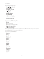
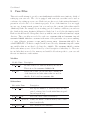
User Manual
Adaptive Multi-Resolution Wavelet-Based Modeling,
Simulation, and Visualization Environment
Code Structure and Setup
(alpha release)
May 8, 2007
Modeling, Simulation, and Visualization Environment
1
Introduction
Welcome to the world of numerical modeling using the computationally efficient, dynamically
adaptive, Adaptive Wavelet-Collocation Method (AWCM). The numerical algorithm used in
this method is a finite difference based scheme which uses an adaptive wavelet transform in
conjunction with a prescribed error threshold parameter ǫ to determine which grid points
are needed in the solution. By reducing the number of points needed to solve the numerical
solution, the computational cost is significantly reduced resulting in large data compression.
It has been shown that the error within the solution using this technique is bounded by Cǫ,
where C is usually around ∼ 10 (@warning Citation ‘donoho:1992’ on page 1 undefined).
The error threshold parameter ǫ is prescribed beforehand and is used throughout the entire
simulation. It is recommended that the equations be non-dimensionalized for the numerical
algorithm even though L∞ and L2 normalization techniques are used to further scale the
equations. Typical values for the error threshold parameter ǫ range from 10−6 to 10−1 ,
anything below that range usually decreases the compuational efficiency significantly and
anything above that range has significant error that isn’t easily ignored.
The wavelets used in the wavelet transform can be of any even order of accuracy. Each
wavelet’s accuracy is determined by its stencil size, which is typically prescribed in terms of
the number of points used on each side of the point being calculated. Two stages are used to
calculate the wavelet coefficients; a predict stage and an update stage. The number of points
used on each side in the predict stage are called n_predict and the number used during the
update stage are called n_update. In order to ensure the wavelet properties are maintained,
these two parameters should be equal. Similarly, the stencil size for derivative calculations
is prescribed in the same way. Since the wavelets support is naturally centered, the default
setting for derivative calculations is centered as well. The stencil size for a centered derivative
calculation is 2*n_diff where n_diff is the number of points on each side of the location
being calculated. In practice, all three of these parameters are normally the same to achieve
the highest performance and accuracy.
THE AWCM is set up to solve two main types of partial differential equations (PDEs),
elliptic and time evolving or a combination of the two. The elliptic solver can be used to
solve for the initial condition used in a time evolving problem, or can be used solely on its
own. The time evolving portion can also be supplied with an analytical initial condition and
uses either a Krylov or Crank-Nicolson implicit time integrator. Due to the fact that the
time integrators are implicit algorithms, the only time constraining parameter used in the
code is the CFL condition. As long as CFL ≤ 1 the time integrator should function properly
and the solution will remain within the anticipated error margin.
The grid used with the AWCM can be described as if it had two parts, a base grid to build
upon and several further levels of refinement. The level of resolution at any point in time is
described by the variable j_lev. For any simulation, minimum j_min and maximum j_max
1
User Manual
levels of resolution must be specified. The base grid size is prescribed with the M_vector
variable. Combining all of these parameters will give a grid with a minimum and maximum
grid sizing. For example, if a 2-D simulation is to be performed using a domain of dimension
2.0 × 1.0 with periodic boundary conditions in the y-direction and the aspect ratio is desired
to be unity, the following could be a suitable grid setup:
dimension = 2
Mvector = 8, 4, 0
periodic = 0, 1, 0
jmin = 2
jmax = 7.
This sets the dimensionality of the simulation to a 2-D simulation so that the third index in
the M_vector and periodic vector are ignored. The base grid of 8 × 4 is on the j_lev=1
level, but because the solution is not periodic in the x-direction the base grid is really
9 × 4. However, the minimum level of resolution is set to be 2 so the coarsest grid possible
in this simulation will be Mvector 2jmin−1 + periodic = 17, 8 corresponding to a grid spacing
h = 2/16 = 1/8 = 0.125 and a total of 136 points. Similarly the finest grid possible in
this simulation will be Mvector 2jmax−1 + periodic = 513, 256 corresponding to a grid spacing
of h = 2/512 = 1/256 ≃ 3.9 × 10⁻³ and a total of 131328 points. Throughout the solution
the resolution will change such that the finer levels of resolution will be used in the regions
where localized structures are present. If the simulation only uses 10, 000 points it would
only be using 7.6% of the points available and have a compression ratio of 13.1.
The rest of this manual will try to familiarize you with the codes organization and how
a user can create their own simulations. A brief overview of the codes organization will be
given in Section 2 and point out which files need to be modified and others that should be
left untouched. Section 3 will demonstrate how to obtain the code using subversion, set up
a makefile, compile and run the code. Section 4 will show how to compile and use the post
processing tools for data visualization. Finally Section 5 will proceed with the details of the
case files, how they are used and how to customize them to any particular situation.
2
Modeling, Simulation, and Visualization Environment
2
Code Structure
2.1
Overall Code Organization
The Adaptive wavelet collocation method (AWCM) solver consists of two parts:
1. elliptic solver and
2. time evolution solver.
The elliptic solver can be used either to solve general elliptic problems of the type Lu = f
or as a part of initial condiitons, where a linear system of PDEs is solved during each
grid iteration instead of prescribing u analytically. The adaptive grid refinement procedure
provides a way to obtain the solution (initial conditions) on an optimal (compressed) grid.
The pseudocode for both the iterative global elliptic solver and the time evolution problem
are shown below.
3
User Manual
initial guess (m = 0): um
G≥m
k and
h
i
while m = 0 or m > 1 and G≥m 6= G≥m−1 or kf J − LuJ≥ k∞ > δǫ
m=m+1
perform forward wavelet transform for each component of um
k
for all levels j = J : −1 : 1
create a mask M for |dµ,j
l | ≥ ǫ
end
extend the mask M with adjacent wavelets
perform the reconstruction check procedure
construct G≥m+1
if G≥m+1 6= G≥m
m+1
interpolate um
k to G≥
end if
solve Lu = f using Local Multilevel Elliptic Solver.
end
Algorithm 1. Global Elliptic Solver.
initial conditions (n = 0): unk and G≥n
while tn < tmax
tn+1 = tn + ∆t
integrate the system of equations using Krylov time integration to obtain un+1
k
n+1
perform forward wavelet transform for each component of uk
for all levels j = J : −1 : 1
create a mask M for |dµ,j
l | ≥ ǫ
end
extend the mask M with adjacent wavelets
perform the reconstruction check procedure
construct G≥n+1
if G≥n+1 6= G≥n
interpolate un+1
to G≥n+1
k
end if
n=n+1
end
Algorithm 2. Time Evolution Solver.
4
Modeling, Simulation, and Visualization Environment
2.2
Code Categories and Files
The code consists of FORTRAN and Matlab files. The FORTRAN code saves results in
terms of active wavelet coefficients, while Matlab files are set up to read output files from
the FORTRAN code, perform an inverse wavelet transform, and visualize the results.
The FORTRAN files can be divided into the followqing categories:
Case Files:
user case.f90
user input.inp
where the user_case is the name of a specific case set up by user that can be located in
any directory, while user_input in the user defined input file. Note that the same case can
have multiple input files.
Core Files:
wlt 3d main.f90
wavelet 3d.f90
wavelet filters.f90
elliptic solve 3d.f90
time int cn.f90
time int krylov 3d.f90
This category inculdes all the core files for the Adaptive wavelet collocation method. We
don’t need to modify any part of these files.
Data-Structure files:
wavelet 3d wrk.f90
wavelet 3d wrk vars.f90
Shared Variables Files:
shared modules.f90
wavelet 3d vars.f90
elliptic solve 3d vars.f90
wavelet filters vars.f90
io 3d vars.f90
This category includes all the variable only modules, i.e. these modules contain no functions
or subroutines.
5
User Manual
Supplementary Utility Files:
input files reader.f90
read init.f90
read data wray.f90
io 3d.f90
util 3d.f90
default util.f90
vector util.f90
endienness big.f90
endienness small.f90
reverse endian.f90
Supplementary FFT Package Files:
fft.f90
fftpacktvms.f90
fft.interface.temperton.f90
fft util.f90 spectra.f90
ch resolution fs.f90
These supplementary files are located in subdirectory FFT and, if necessary, can be used for
extracting statistics in homogeneous directions.
Supplementary LINPACK files:
d1mach.f
derfc.f
derf.f
dgamma.f
dgeev.f
dgels.f
dqage.f
dqag.f
dtrsm.f
dum.f
fort.1
gaussq.f
needblas.f
r1mach.f
zgetrf.f
zgetri.f
6
Modeling, Simulation, and Visualization Environment
Visualization Files:
c wlt 3d.m
c wlt 3d movie.m
c wlt inter.f90
inter3d.m
mycolorbar.m
mycontourf.m
c wlt 3d isostats.m
vor pal.m
These are used to visualize the output results. All these files are contained in subdirectory
post_process.
7
User Manual
3
Getting Started
3.1
Obtaining the Source Code
Currently, the most efficient means of obtaining the code is through the use of Subversion.
The use of Subversion allows you to keep your code up to date with the current release without starting all over again. Subversion is available for download at http://subversion.tigris.org
and documentation is available at http://svnbook.red-bean.com.
Once you have subversion installed, make a directory where you want to put the source
code directory called wlt_3d. Move into this directory and use the command
svn checkout https://www.cora.nwra.com/svn/wlt/branches/NASA
You will be asked for a login name and password, you should have this information already.
Enter the information and the import will commence.
It is important that you do not modify any of the files in the main source code. If you
do, the next time a newly released version of the code will conflict with the changes you
have made. It is important that you create your own case files and edit those exclusively
so that you do not introduce any conflicts. If you do find a bug in the main source code,
please send an email to [email protected] so that the problem is properly resolved.
If these guidelines are followed, each time an updated version is released
When an update does become available you can see what files have been changed beforehand by running the command svn status -q from the source directory. The -q option
suppresses output associated with files that are not under version control. Then to proceed
with updating the changed files run the command svn update and you will have the latest
release. If after updating to the latest release there are problems and your code will not
run anymore you can perform and svn revert and the code will be restored to its previous
version.
3.2
Compilation and Execution
The source code is always compiled from the source directory regardless of which case file
executable you are creating. There are three arguments that must be passed to gmake in
order for it to know what to do. First of all, the compiler needs to know which database
to use for storing the data. As of now, the main database in use is db_wrk, but db_tree
and db_lines will be available soon. The next argument is which case you are going to run.
Since the compilation is done from the source directory, the path to the case file needs to be
specified and the executable will be placed in that directory. The path can be specified as
an absolute path or relative to the source directory.
Before attempting to compile anything a makefile must be created specific to your computer. Under the source directory is a subdirectory called makefiles.machine_specific.
8
Modeling, Simulation, and Visualization Environment
Inside this directory are numerous different makefiles all in the form makefile.some_name.
The makefile in the source directory references the makefiles in this directory through the use
of an environment variable WLT_COMPILE_HOSTNAME. You will need to create an environment
variable called WLT_COMPILE_HOSTNAME and set it equal to your some_name. You will also
need to copy one of the makefiles in the makefiles.machine_specific directory that is
similar to your computer’s configuration and rename the file makefile.some_name. Make
sure to make any changes necessary to the names of the compiler and flags so that it will
work on your machine. Once all this is done, gmake will know what to do when you compile.
3.3
Elliptic Solver Example
There are several test cases provided with the code and are located in the TestCases directory. In order to demonstrate how to successfully compile the code we will start with the
EllipticTest1. From the source directory, if you move into the TestCases/EllipticTest1
directory and list the files you will see the following list of files along with some others that
aren’t of importance
case elliptic poisson.f90
case elliptic poisson.PARAMS.f90
results (directory)
test in
showme3D.m
From looking at the different files one can conclude that the case name is case_elliptic_poisson.
As of now the exact syntax used to compile is
gmake DB=databaseName CASE=[path of case]/caseName wlt_3d.
Remember that this is always done in the source directory. For our example [path of case] is
TestCases/EllipticTest1, the case name is case_elliptic_poisson, and we’ll be using
the database db_wrk. The following syntax should successfully compile the code
gmake DB=db wrk CASE=TestCases/EllipticTest1/case elliptic poisson wlt 3d
Make sure to add the target wlt_3d at the end so the compiler will know what to do. Once
the code has finished compiling the executable will be located in the case directory and will
be called, in this example, wlt_3d_db_wrk_case_elliptic_poisson.out. If we move to the
case directory the case can be executed by running the executable and specifying which input
file is to be used as an argument. The input files are located in the test_in subdirectory.
For example, if we wanted to run the 2-D test problem we would use the following command
9
User Manual
./wlt 3d db wrk case elliptic poisson.out test in/base.inp
It should be noted at this time that during the compilation step an important file was
overlooked, which is the case_elliptic_poisson.PARAMS.f90 file. Inside this file are two
parameters needed by the database in order to construct the databases size and dimensions.
If this file is absent the compiler will fail. However, a run time error can occur if the
parameters are not set large enough to handle the input file’s dimensions and number of
variables being stored. Inside this file the parameter max_dim is set to 3. This allows the
database to allocate enough room to run both the 2D and 3D input files. The number of
variables is also set to 10 (n_var_db=10), which is large enough to handle the 3D case with
some extra variables stored. For the 2D case it would be possible to change max_dim to 2
for increased performance, but it is set to 3 for now so that both cases can be run without
changing this file.
3.4
Post Processing
Once you have succesfully run the test case from within the test case directory, the output
files will be stored in the results subdirectory. The output files have the file extension .res.
In order to view the output files in MATLAB, the post-process file c_wlt_inter.f90 needs
to be compiled. From the source directory compile all the needed files with the target
inter using the command gmake DB=db_wrk inter. The executable created is located in
the post_process directory.
10
Modeling, Simulation, and Visualization Environment
4
Data Visualization
Once you have compiled and run your test case and compiled the post processing executable
c_wlt_inter.f90 discussed in Section 3.4 you are ready to view your results files saved in
the results/ subdirectory. There are a few ways to visualize your results now. In the past,
MATLAB has been the primary data visualization tool. Over the past year or two new
visualization tools have been under development, which are capable of 3-D volume rendering
and will be introduced in the following subsections.
4.1
MATLAB Visualization Tools
In order to view the output files using MATLAB you must return to the case directory. Once
you are in the case directory, open the file showme3D.m. Make sure to edit the post_process
directory to its correct location on your computer. Once this is done, you are ready to visually
view the output using MATLAB. Executing showme3D within the MATLAB command
window should read the data from the specified file within showme3D.m.
If you look at the showme3D.m file further, you will notice down near the bottom all of the
arguments used to call the plotting function c_wlt_3d are briefly explained. At the bottom,
a call to this function is shown with each argument defined for you. The first argument
in this list is the file name channel_compressible_test. You will find this matches the
name in the channel_compressible.inp file. The j_range is the range of resolution that
MATLAB will use to plot your solution. The bounds argument determines the domain that
will be plotted.
The figure is set to plot the solution using a contour plot. If you would like to see the
grid, you must set the figure type to grid. The plot_comp variable is the component of the
solution that you want to plot. This is defined in the channel_compressible.f90 code.
The station number is which output step you are plotting. In this case, it is set to 100,
which is the final output time for this case.
4.2
More Data Visualization: Res2Vis
A tool is available to transform AWCM code result files into VTK, PLOT3D, or CGNS
formats for further visualization with ParaView, VisIt, Tecplot, or similar software. To
compile the tool, specify the database type and the case name as usual; the compilation target
will be vis instead of wlt_3d.. The tool will be found in the test case executable directory,
e.g in TestCases/CASE_NAME/ under some generic name res2vis_DATABASE_CASE.out.
Type ./res2vis for the complete manual. In short, at least two file names have to be
provided to the tool: the AWCM result file name, and the base name for the output file. A
VTK unstructured mesh binary output file will be generated by adding .vtk suffix to the
11
User Manual
provided base output name. An optional flag -p will produce PLOT3D binary output, by
using .xyz and .q suffixes. Use optional flag -c to generate CGNS file.
It should be noted that ParaView has no problems with reading VTK unstructured mesh
files. The same is true for Tecplot reading CGNS files. As for the ancient PLOT3D format,
Tecplot will auto detect file structure for ASCII files only. For binary files, file structure has to
be specified manually as “Plot3D Function”, “Unstructured”, not “Multi-Grid”. Moreover,
Tecplot known to have problems with reading binary 3 dimensional plot3D files on some
architectures, so use ASCII plot3D or, which seems to be a better solution, CGNS format.
4.2.1 complete manual of res2vis
Usage: res2vis [OPTIONS] [IN_FILE] [OUT_FILE]
res2vis [OPTIONS] [IN_DIR] [IN_FILE] [OUT_DIR] [STATION_BEGIN] \
[STATION_END] [STEP]
Data options:
-t
apply inverse wavelet transform to show the data values
(wavelet coefficients are displayed by default)
-i
use integer space coordinates, according to the mesh
(coordinates are real by default)
Output formats:
-v
VTK file (default)
-p
plot3D files
-c
CGNS file
Additional output formats:
-a
VTK, plot3D: the output file is ASCII (binary by default)
-r
VTK, CGNS: use tetrahedra (blocks will be written by default)
Additional filtering, before the transform:
-e threshold_value number_of_variable_for_threshold
-l maximum_level_to_use
Files:
input_result_file output_filename
input_directory generic_input_filename output_directory first_station \
last_station step
Example:
res2vis -vpa -e 0.15 4 ../res/input.0001.res out
produce both VTK and plot3D ASCII files (out.vtk, out.q, out.xyz)
and the data will be filtered by applying the threshold 0.15
to the variable number 4 of the result file,
res2vis res/ in. ./ 0 6 3 -t
12
Modeling, Simulation, and Visualization Environment
writes data as VTK files (in.0000.vtk, in.0003.vtk, in.0006.vtk)
into the current directory for each of the input file from the directory ./res/
(in.0000.res, in.0003.res, in.0006.res)
13
User Manual
5
Case Files
This section will attempt to provide some familiarization with the more intricate details of
setting up your own case. The code is equipped with some test cases that can be used as
a reference for setting up a new case. Each test case has a set of subroutines that must be
present in order for the code to function properly. If one of the functions does not apply
in your case, it must remain present, but you can leave the contents (other than variable
definitions) blank. For example, if you are using periodic boundary conditions, you can leave
the details in the user_algebaic_BC function blank, but do not delete the function itself.
Each case should have its own separate directory with its own case files and results/ output
directory. Three case files are needed for each case: casename.f90 and casename.inp and
casename.PARAMS.f90 where casename is the name of the particular case your are running,
e.g., case_elliptic_poisson or case_small_vortex_array. Casename.f90 will be the
actual FORTRAN code that is compiled in the source directory. Casename.inp will contain
any variables that are not hard coded into the .f90 file. The casename.f90 file contains
all the subroutines you see below followed by a brief description of what they do. There are
two modules that are needed for memory and variable allocation specific to your case and
the rest are functions or subroutines.
Modules
Module Name
Description
user case db
Module created for database memory allocation.
This is stored in casename.PARAMS.f90.
user case
This is the actual case module that contains all
of the functions and subroutines that are used in
this file. It is located in casename.f90.
Subroutines
Subroutine Name
Description
user setup pde
Sets up the number of variables that are integrated or interpolated on the initial time step and
any subsequent step.
user exact soln
Stores the exact solution in memory.
user initial conditions
Defines the initial conditions if they can be determined analytically.
user algebraic BC
Sets conditions on boundaries
14
Modeling, Simulation, and Visualization Environment
user algebaic BC rhs Specifies the right hand side for boundary
conditions.
user project
Used for Crank-Nicolson time integration to get
projections of variables that are needed for integration, but not actually integrated with the actual solver.
Laplace
Sets up the Laplacian.
Laplace diag
Sets up the diagonal terms for the Laplacian
Laplace rhs
Sets the right hand side for the Laplacian
user rhs
Sets the right hand side of the PDE being solved
user Drhs
Sets the Jacobian of the right hand side of the
PDE.
user Drhs diag
Sets up the diagonal terms for the Jacobian when
the Crank-Nicolson time integration method is
used.
user chi
This is your boundary used for immersed flow
boundary conditions.
user stats
Any user specified statistics that need to be calculated to analyze new data can be calculated here.
user cal force
Used to calculate lift and drag on any bodies in
the flow (Not implemented yet).
user read input
Any user defined variables defined in the casename.inp file are read through this subroutine.
user additional vars
Where any additional variables are calculated.
user scalar vars
Any scalar non field parameters that need to be
calculated can be done here.
user scales
Used to override the default scales routine.
user cal cfl
Override default cfl condition and use user created
condition.
15
User Manual
5.1
CaseFile.f90 Details: Channel Compressible
Now that we’ve taken a general look at how the case files are structured, let’s look at a
specific case and explain how it is set up. The channel_compressible.f90 case is set up
to solve the Navier-Stokes Equations in a channel which is initially at rest with an upper
wall moving at a velocity of 0.1 and the bottom wall is at rest. The fluid is initially not in
thermal equilibrium with the walls. The domain is periodic in the x-direction with Dirchlet
conditions on the top and bottom boundaries.
5.1.1 MODULE user case
This is the main module that the entire case file is built into. Any variables that you want to
be available globally throughout the entire module should be defined in this section. Below
where it says “case specific variables,” the variable n_var_pressure is declared. As of now,
this parameter must always be declared because the code is set up to solve both compressible
and incompressible flows. Following are some non-dimensional parameters Re, Pra, gamma
and alpha as well as boundary condition parameters T_top and U_wall. As you will see,
these variables are imported from the test_in/base.inp file in the user_read_input subroutine. There are also two other logical parameters that are defined to set up the equations
and how they are solved; NS and NSdiag. NS switches the equations from Navier-Stokes to
Euler equations, .TRUE. for Navier-Stokes and .FALSE. for Euler equations. At this point a
hyperbolic solver capable of resolving shocks with the hyperbolic Euler equations has been
developed but is not implemented yet. It should become available with further updates.
NSdiag should be set to true if NS is true and you are using the Crank-Nicolson time integrator. If the Krylov integrator is used the user_Drhs_diag subroutine is never called and
doesn’t need to be true.
5.1.2 SUBROUTINE user setup pde
In this routine we set the global parameters the main code uses to know how many equations
it is integrating, interpolating, saving and how many variables there is an exact solution for.
The number of variables that are integrated n_integrated is set to dim+2 since we are solving for ρ, ρe, and the momentum equations in dim dimensions. In the test_in/base.inp
file the dimsion parameter is set to dim=2. Leave n_time_levels and n_var_time_levels
as they are. They will soon be phased out. Any additional variables that are not integrated, but you want calculated at each time step set as n_var_additional. As an example,
n_var_additional is set to 1 so that we can calculate the pressure and save it at each time
step. This is totally unnecessary as pressure can be calculated during the post processing
step, but it is performed here purely for demonstration purposes.
The next step is to fill in the variable names according to how we arrange our variables.
16
Modeling, Simulation, and Visualization Environment
We will fill in the variables depending upon how many dimensions there are starting with
density as the first variable, x-momentum as the second and so on.
The grid does not need to adapt to all 5 variables. Pressure (the 5th variable) is simply
found using the 4 conserved variables. Obviously we will only need the grid to adapt to
the 4 conserved variables, so we set n_var_adapt to n_var_adapt(1:n_integrated,0) and
n_var_adapt(1:n_integrated,1) to .TRUE. The 0 index indicates adaptation when setting
up the initial condition and 1 index adapting at each time step afterwards. We also need the
grid to interpolate all of the integrated variables as time moves along as well. Adaptation
means that the grid will evolve based upon a given variable. Interpolation is what needs to
happen in order to add a previous time step to the next. In this case, it is not necessary to
interpolate the pressure so we have set the first 4 variables to be interpolated both at the
initial condition and all time steps thereafter.
We want to save all 5 variables at each write step, so we have set n_var_save as true for
all variables n_var. For the time being, please ignore the time level counters and leave them
the way they are. These will most likely be phased out in the future. An exact solution
exists for this problem so n_var_exact_soln has been set to true. If you find that you need
more points due to a a certain variable, you can create a scaleCoeff < 1.0 to add more
points to that variable. If it is left as 1.0 it will scale the solution in its default manner
according to your error threshold parameter ǫ.
5.1.3 SUBROUTINE user exact soln
This is where we calculate the exact solution. Even though it is called u, it is not the same
u that is used to numerically calculate the solution. The main code takes this u and stores
it as the exact solution somewhere else.
5.1.4 SUBROUTINE user initial conditions
If you know the analytical initial condition, it is set up here.
5.1.5 SUBROUTINE user algebaic BC
Algebraic boundary conditions are set by solving the general equation
Lu = f.
(1)
There are three main subroutines used to solve this equation. The first is user_algebaic_BC.
This subroutine sets up the Lu portion of the equation. As you can see from this example,
Dirichlet conditions are created for both the velocity and energy on the top and bottom
boundaries. The top wall temperature is T_top and the bottom wall is 1.0.
17
User Manual
5.1.6 SUBROUTINE user algebaic BC diag
Since the equation above is solved iteratively, the diagonal terms of L need to be provided.
user_algebaic_BC_diag becomes this term. In this case for Dirichlet conditions they are
equal to 1.
5.1.7 SUBROUTINE user algebaic BC rhs
To finish setting up the equations that need to be solved, user_algebaic_BC_rhs is the
right hand side of the above equation f. In this case the right hand side is zero.
5.1.8 FUNCTION Laplace
This is the elliptic solver portion of the code. It is not used in this case but is demonstrated
in Secion 5.3.
5.1.9 FUNCTION Laplace diag
This is where the diagonal term used in the Laplace equation definition is made. An example
of its use is provided in Secion 5.3.
5.1.10 FUNCTION Laplace rhs
This is where f in equation 2 is defined. An example of its use is provided in Secion 5.3.
5.1.11 FUNCTION user rhs
In the function user_rhs, we need to supply the right hand side of the main governing
equation. The left hand side is the time derivative that we’re integrating and the right hand
side is everything else. This is supplied to the function user_rhs. As you can see, the right
hand side has already been set up for both the Euler and Navier-Stokes equations. In this
test case it will be using the full Navier-Stokes equations because the logical variable NS is
true as described above. For details on how to use the derivative operator c_diff_fast see
Section 5.3.
5.1.12 FUNCTION user Drhs
Since the Crank-Nicolson and Krylov are implicit iterative time integration solvers, we need
to provide a first order perturbation to help the iterative solver converge more quickly. The
user provides this perturbation to the main code through the function user_Drhs. Since
the right hand side has already been defined, finding the perturbation is simply a matter of
applying the linearized theory. In this case the linearized equations are given as an example
for both the Navier-Stokes and Euler equations. If there is a mistake made when entering the
18
Modeling, Simulation, and Visualization Environment
equations into DRHS it may still converge, but it may take a few more iterations. Otherwise,
the solver will continue to iterate without reaching its error threshold criteria indefinitely.
5.1.13 FUNCTION user Drhs diag
When using the Crank-Nicolson technique, a diagonal term needs to be created from our
DRHS. The diagonal term for both the Navier-Stokes and the Euler equations are shown in
the example. Note that this is only for the Crank-Nicolson method. When using the Krylov
integrator this section does not need to be defined because it is not used.
5.1.14 SUBROUTINE user project
This routine is mostly used for incompressible flows where the pressure needs to be tracked,
but not integrated. The Crank-Nicolson method is used with this projection step to ensure
that the velocity vector v remains divergent free. The small_vortex_array case demonstrates this feature more clearly.
5.1.15 FUNCTION user chi
If there is to be an obstacle in the flow using Brinkman penalization, you would determine
your χ function here. If it is equal to 1.0 it is inside the boundary and if it is equal to zero
then it is outside.
5.1.16 SUBROUTINE user stats
After results of a new time step are available, you may want to generate some statistics
based on those results. This function serves that purpose and is called from the main code.
User_stats allows you to make these calculations without touching the main code.
5.1.17 SUBROUTINE user cal force
If an obstacle has been defined in the user_chi function, the lift and drag are calculated
here.
5.1.18 SUBROUTINE user read input
In the subroutine setup_pde we defined our variables Re, Pra, gamma, alpha, T_top and
U_wall. This is where we read them into the module from the test_in/base.inp input file.
Each variable is read in separately with its own input_real command. The input_real
command is only used to input real type numbers. If you want to read an integer you would
use input_integer. The parameter ’stop’ tells the code that if that variable is not read
19
User Manual
properly, it will stop the code execution. If you look in the test_in/base.inp file, you can
see how to set up your own variables just like these.
5.1.19 SUBROUTINE user additional vars
Any additional variables that aren’t integrated but are stored in the main storage array u
are calculated here. In our case, we are storing pressure in the n_var_pressure portion of
u that we created in setup_pde. Again, normally it would be better to calculate pressure in
the post processing step, but we are storing it here as an example.
5.1.20 SUBROUTINE user scalar vars
If there are any scalar (non-field) parameters defined at the beginning of the module that
need to be calculated, they should be handled here.
5.1.21 SUBROUTINE user scales
In the situation that you wish to override the default scales routine in the main code, you
would do that here.
5.1.22 SUBROUTINE user cal cfl
If you wish to override the default cfl condition you would do that here. The subroutine
get_all_local_h returns the grid spacing for all points on the active grid. We then determine the cfl for each grid point and ultimately select the largest as cfl_out.
5.2
CaseFile.inp Details: Channel Compressible
The input file is where all of the variables that are not hard coded into your case file are
stored. As seen in the previous section, any variables you need are read using an input_real
or input_integer statement. For the channel_compressible case, we ran a 2-D NavierStokes simulation. Inside of the test_in/base.inp file you will see all of the parameters
that are needed to run this case.
The first several variables pertain to input output and initialization parameters. file_gen
is whatever you want the output in the results subdirectory to be saved as. There are three
main ways to initialize your initial conditions. The first way is to use an analytical solution
which you provide in the user_initial_conditions subroutine. Another way is to restart
a previous run from a given output time. In order to do this you simply specify the name of
the file name for IC_filename, set IC_restart=T and specify the output time to start with
with IC_restart_station. A third way is to use some other file for the initial conditions
which may or may not match the current configuration of your case. You can take the input
20
Modeling, Simulation, and Visualization Environment
data and manipulate it to match your current case and then start your simulation. In order
to start with this configuration you would make sure IC_restart=F, set IC_from_file=T
and specify the IC_filename as in the restart case. It should be noted that there are multiple
ways in which the IC file can be formatted and you must specify its format beforehand with
IC_file_fmt. You also must be sure to specify how the output will be formatted, binary
or ascii. The unformatted binary version works much faster and takes up less disk space so
that is the recommended method.
The domain size is specified with coord_min and coord_max. We have specified three
different dimensions in the case that dimension is set to 3 then the input file is ready to use. In
the case of our 2-D run, it simply ignores the extra dimension. In order to avoid problems at
the boundaries, it is sometimes necessary to specify a coord_zone_min and coord_zone_max.
The way these parameters work is that if you pick a coord_zone parameter to be inside of the
domain, all points on the finest level of resolution will be included between that coordinate
and the boundary. The max portion corresponds to the upper side of the domain and the
min portion corresponds to the lower side.
The overall solution error is controlled with the parameter ǫ. The code has been set up
to allow the use of two different ǫ’s depending on your particular situation. Eps_init can
be used as a separate initial thresholding parameter for eps_adapt_steps number of steps
before using the regular eps_run parameter. In our case there is no difference between the
two.
Setting a threshold parameter ǫ is only effective on its own if all integrated variables are
normalized to the same scale. This is usually not the case and a scaling method Scale_Meth
needs to be specified to keep the relative error in check. In our channel_compressible
case, all the equations are normalized with a mean value of zero so choosing Linf error as
the scaling method is not a bad choice. However, in other situations it may be better to
use an L2-norm error or possibly a RMS scaling method. In some situations, the time scales
can change very rapidly which causes your scales to rapidly vary as well. Since this can
sometimes be problematic, a temporal filter has been provided to slow the speed at which
these scales change scl_fltwt. This parameter has the range of [0, 1] where zero corresponds
to no filtering and 1 corresponds to being completely based upon historical scales.
In every simulation, the minimum and maximum grid size needs to be specified by setting the minimum and maximum levels of resolution, J_MN and J_MX, as well as the initial
M_vector. In our case the M_vector is [4, 4] and J_MN and J_MX are 2 and 4. The minimum
grid size is M_vector*2^J_MN+prd (17x16) and the maximum grid size is M_vector*2^J_MX
(65x64). In our case J_MX is set relatively small because it is a test case and we want to limit
the level of resolution for computational reasons.
The boundaries are set to be periodic in the x-directiona and has Dirchlet conditions in
the y-direction. Although our grid is adaptive, the grid spacing on each level of resolution
remains constant throughout the domain, hence the grid is called uniform.
21
User Manual
The parameters i_h and i_l specify the order in which boundaries are stored in the u
array and what type of boundary conditions will be imposed, either algebraic or evolutionary.
The order of the wavelets used are specified with N_predict and N_update. These parameters determine how many points are used on either side of the point being interpolated. In
our case they are 2, so we are using 4th order wavelets. N_diff is the number of points used
on each side of a centered difference scheme to calculate the derivatives. Since N_diff is 2,
we are using a 4th order central differencing scheme. Generally it is wise to make all three
of these parameters the same.
The next two parameters IJ_ADJ and ADJ_type deal with the fine details of how the
code chooses to pick points. It’s generally good to leave IJ_ADJ as 1 for all three levels. If
ADJ_type is set to 0 it will use less points and run faster, but if convergence becomes an
issue, set this parameter to more conservative. This alone may solve a convergence issue
when faced with one.
If non-periodic boundary conditions are used, BNDzone should normally be set to true.
It will use the parameters coord_zone_min and coord_zone_max when this is on. BCtype
specifies the type of boundary conditions used if custom ones are not needed. The time
integration method chosen in this example to be the implicit Krylov scheme. It can also use
an implicit Crank-Nicolson technique.
The next several variables all involve temporal aspects of the code. The beginning and
ending of the simulation are specified with t_begin and t_end. The initial time step used
to start off the run is dt. The minimum and maximum time steps are set with dtmax and
dtmin. Dtmin can serve as a stability indicator in that many times the time step will become
smaller and smaller as the solution begins to diverge. If dt drops below dtmin it is usually
because there is a problem. dtwrite specifies the time interval used for writing output to
the ouput files. An additional feature has been recently added to the code which allows
you to force the solution to be written after every time step. This is done by creating a file
named [filegen].force_write in the case directory, where filegen is the basename for
your output files created in the results directory. After each time step, the main executable
checks for the existence of this file. If the file exists it will write the output from the time
step that was just executed, otherwise it will wait until the next t_write corresponding to
the specified dtwrite. The parameter t_adapt can be used to make all time steps below
t_adapt of the same size and once t is greater than t_adapt, the time step is free to change
with the solution. The maximum and minimum cfl conditions are set with cflmax and
cflmin. The minimum cfl serves as a trigger for stopping the time integrator in the case
that the solution is diverging.
In the channel_compressible case example, we need to define several paramters. They
are set here for no reason in particular. Note that the order in which variables are declared
is not important.
The variable Zero_Mean is for cases in which you want the mean value of the first 1:dim
22
Modeling, Simulation, and Visualization Environment
variables to remain zero. The next several variables are for the Krylov time integrator and
the elliptic solver. It is best not to touch these unless you have a good understanding of how
it works and are having problems with the way the current paramters are set up.
If you wish to insert an object into the flow using Brinkman Penalization you would set
the obstacle variable to T. Its location, size and movement directions can all be specified
using the various different variables. You would probably create a few of your own variables
and then make sure to define that objects domain in the user_chi subroutine. The rest of
the variables are other integration parameters that should normally be left alone.
5.3
CaseFile.f90 Details: Elliptic Solver
Another important functionality of the code is the ability to efficiently solve elliptic problems. The previous example focused on the time integration portion and this example will
focus on how to solve an elliptic problem. There is a test case set up in the directory
TestCases/EllipticTest1 with a case name case_elliptic_poisson.f90.
The following subsections will discuss how the elliptic test case is configured.
5.3.1 MODULE user case
As in the previous example this is the main module that the entire case file is built into.
Any variables that you want to be available globally throughout the entire module should be
defined in this section. You can see that since we are solving Poisson’s equation the number of
variables stored in the database is n_var_db=1. The number of possible dimensions max_dim
is set to 3 to allow all possible configurations.
5.3.2 SUBROUTINE user setup pde
Again, in this routine we set the global parameters the main code uses to know how many
equations it is integrating, interpolating, saving and how many variables there is an exact
solution for. For this case the number of variables being integrated is 1, there are no additional variables being stored and we do have an exact solution to compare with. No pressure
needs to be stored because the time evolution part of the code is not being used.
5.3.3 SUBROUTINE user exact soln
There is an exact solution to this problem which is defined in this routine.
5.3.4 SUBROUTINE user initial conditions
When the elliptic solver is used, the user_initial_conditions subroutine functions as the
main place to set up the problem. The elliptic solver uses the subroutine Linsolve to solve
23
User Manual
the general equation
Lu = f.
(2)
In this case the right hand side f is set up and passed directly to the subroutine Linsolve.
In other cases f can be defined using the Laplace_rhs function. The other functions that
are passed in Linsolve are Laplace and Laplace_diag. These functions will be defined
in the following sections. Once Linsolve has completed its iterations, the solution will be
printed to an output file and the code will stop.
5.3.5 FUNCTION Laplace
This is the elliptic solver portion of the code. This is run before any time evolution ever
begins. It is created to solve equation 2. The Laplace subroutine sets up the operator on the
left hand side of this relation. It is important to note that the boundary conditions for the
elliptic solver are specified within this function and the next two following. In this case we
are setting up the Laplacian as the operator. Two seperate techniques are set up to calculate
the Laplacian. One way is to simply take the second order derivative in dim-dimensions or
the other is to take the divergence of the gradient. It switches between the two with the
parameter divgrad, which is set to false in this case, so the default is the simpler second
order derivative.
The derivatives are calculated with the function c_diff_fast. The syntax used in this
subroutine is as follows
CALL c_diff_fast (u, du, d2u, jlev, nlocal, meth, 01, ne_local, 1, ne_local)
You’ll notice that the first three arguments are u, du and d2u corresponding to the
function that is being differentiated, the variable to ouput the first order derivative to and
the second order derivative respectively. The next variable is jlev, which is the current
level the solution is on. nlocal is the number of points being used and stored in u per
variable. Another important variable is the method, meth, meth1 and meth2. You’ll notice
for the simpler second derivative case meth=0, where as for the divergence of the gradient
method, meth1=2 and meth2=4 are used. This is so that one sided differencing can occur. For
example meth=2 corresponds to backwards in space differencing whereas meth=4 corresponds
to forwards in space differencing. Another important parameter is the parameter that follows
meth. This can be either 10, 01 or 11. It is simply a logical indicator as to which derivative
is to be computed where the first and second indices correspond to the first order and second
order derivatives respectively. Next comes ne_local, which is just the number of variables
stored in the array u. The next parameter is set to 1 in this case, but this value corresponds
to which variable stored in u you want to differentiate. It can be a single value, or it can be
a list of values, say 1:n_var. This is better demonstrated in user_rhs of Section 5.1.
At the bottom of this subroutine the boundary values are specified for all of the different
types of boundary conditions. In this case they’re all specified to be Dirichlet conditions.
24
Modeling, Simulation, and Visualization Environment
5.3.6 FUNCTION Laplace diag
This is where the diagonal term used in the Laplace equation definition is made. A function
similar to c_diff_fast, yet only gives the diagonal terms is c_diff_diag.
5.3.7 FUNCTION Laplace rhs
This is where f in equation 2 can be defined. Since f is already defined in user_initial_condtions,
is passed directly to Linsolve and is not required anywhere else in the code, it does not
need to be here.
5.3.8 SUBROUTINE user read input
No parameters are read from the input file for this example.
5.3.9 SUBROUTINE user scales
The default scales are used for this case
5.4
CaseFile.inp Details: Elliptic Solver
All of the paramters are set up in the same way as the previous example except that t_end=0.
This prevents the time integration from beginning and outputs only the final solution to the
elliptic problem in the results/ subdirectory. The output file will end in 0000.res since it
is the first output file of problem.
25
User Manual
6
Creating Your Own Cases
Before moving forward, grabbing a test case the looks similar to what you want to do and
modifying it to suit your needs, it would be better to create your own directory outside of the
source code where you will not be editing files under subversion management. There are a
couple reasons for this. One is that whenever an update is available, you won’t have a conflict
with the new incoming version and the second is that if you make a mistake somewhere you
always have a working copy that you can return to for reference. It is recommended that you
create another sister directory next to the main source directory where you will put your new
cases. When compiling you can still use relative paths or you can use absolute paths, which
ever you prefer. You will also have to make sure that you edit the path for showme3D.m to
reference the correct directory as well.
26
Modeling, Simulation, and Visualization Environment
7
NASA Specific Modules
There have been five new modules created specifically for NASA’s purposes. They are
located in TestCases/dns. They are organized into two different files, dns_module.f90
and urans_module.f90. dns_module.f90 simulates flow around a cylinder with the flow
moving from left to right at Ma = 0.2 using the compressible Navier-Stokes equations and
an acoustic Reynolds number of Re = 1000. urans_modeule.f90 solves the same problem
but uses the k − ω turbulence model. The model is incorporated in the user_case module in
the user_rhs, user_Drhs subroutines. Since it is using the Krylov solver, user_Drhs_diag
is not specified. In this case the Reynolds number is Re = 106 . Both of these cases use the
Freund Boundary method to prevent reflections from occuring at the domain walls. Both of
these files include the additional modules needed by the main case file that uses them except
for the far field acoustics predictor FWH, which is located in the source directory. There are
a totoal of five new modules: Brinkman_penalization, Freund_boundary, wlt_FWH, DNS
and uRANS. They are explained in the following sections
7.1
Brinkman Penalization
This module is used to deal with the complex obstacles inside the flow field. It uses Brinkman
Penalization to add semi-porous obstacles into the flow field which act as solid bodies to
appropriately divert the flow. Inside of both dns_module.f90 and urans_module.f90,
you will find the boundary is defined in two different sections. First it is defined in the
Brinkman_obstacle subroutine inside the Brinkman_penalization module and also in the
initial_obstacle subroutine inside the user_case module. These two subroutines serve
very different functions. initial_obstacle serves as a function that the grid can adapt to
since in the initial conditions all the flow variables are constant. Brinkman_obstacle defines
the obstacle that is used by the Brinkman_penalization module to add the penalization
terms to the fluxes calculated in user_rhs, user_Drhs, etc. The module is activated by
the flag Brinkman_active located in the dns_module.inp file. It uses one parameter, nita,
which determines the porosity of the obstacle. The variable nita should be a small value,
approximately 0.01 or smaller to ensure that the obstacle is close to being a full solid. As
of now, the obstacles cannot be fully discontinuous heavy-side functions. Instead hyperbolic
tangeants are used. In the future it will be possible to use heavy-side functions and the
boundary will be specified with the user_chi function in the user_case module.
7.2
Freund Boundary
The Freund’s buffer zone is used to avoid the spurious reflections from the domain walls. It
basically works by accelerating the flow to supersonic speeds near the boundaries by adding
volumic terms to the governing equations. In order to activate this feature you simply set
27
User Manual
the logical flag Freund_active located in the dns_module.inp and urans_module files to
TRUE.
7.3
FWH
This module is used to predict the far field acoustics. As of now it is only available in 2-D, but
3-D will be available in the future. In order to use this module, there is a logical flag inside of
the input file additional_nodes_active. If the prediction is needed, set it to TRUE. When
the module is activated you must create a seperate directory inside of the results directory
called filegen, which is the base name of your output files specified in your input file. The
additional far field prediction files will be stored in that subdirectory. In addition, the patches
used to predict the far field acoustics must be specified in the input file as well. The number
of patches used is specified by n_additional_patches and the locations of the points used to
create the n-point polygon are specified with the x_patches and y_patches parameters. The
final paramter that must be specified is j_additional_nodes. This paramter determines
what level of resolution will be used on the contour to calculate the far field acoustics. This
parameter must always be smaller than the finest level of resolution.
7.4
DNS and uRANS
These two modules are basically implemented in the two different dns_module.f90 and
urans_module.f90 FORTRAN files. Both are set up for fluid flow using the Navier-Stokes
equations. The only difference between them is that the uRANS file uses the k − ω model
in the user_rhs, user_Drhs, and user_Drhs_diag subroutines.
28
Modeling, Simulation, and Visualization Environment
8
Code Development
A test suite is available for code developers. The structure of the test suite is the following.
make tests from the source main directory will execute a) the tests for the test cases, b)
the tests for the post-processing tools and subroutines. Complete testing may take up to
several hours depending on your system and test input parameters.
8.1
Tests for the test cases
All the tests for the test cases could also be run from TestCases directory as
cd TestCases; gmake tests
It is also possible to start different tests separately as
cd TestCases; gmake test1; gmake test2; gmake test3
The detailed description can be found in TestCases/README and TestCases/util/README
files. The files in directories TestCases/*/test_in contain control parameters affecting the
execution of the testing scripts for each test case. Examine the files for details.
In short, tests for the test cases are performed by the scripts from TestCases/util
directory RUN.sh, RUN 2.sh, and RUN 3.sh. The first script, RUN.sh performs compilation
of various targets for different data bases and test cases (Cartesian product of list of targets,
list_ta, list of data bases, list_db, and list of test cases, list_ca). All three lists are
defined inside the file RUN lists.txt, which is sourced from all RUN*.sh scripts. The major
output of the first test is inside the file
TestCases/TEST LOGS/COMPILE.log
It contains minimum information regarding successful compilation of test cases.
The second test, performed by RUN 2.sh script, examines execution and restart capabilities of the code. The major output can be found inside the file
TestCases/TEST LOGS/RUN.log
and inside the files TEST.REPORT in test case directories. The control parameters for
the second test for each test case can be found in test case subdirectory test in in the file
local test parameters.txt Input files will be generated according to the provided rules in
the same test case subdirectory test in in the file rules.inp Examine the mentioned files for
details.
The third test is performed by RUN 3.sh script. It examines code execution for different combinations of input parameters. Instead of predefined during the second test inputs the
third test generates inputs by itself. Input generator uses numerous input rules parameters.txt
29
User Manual
file from the test case subdirectory test in to produce input files with all the combinations
of given parameters within a predefined range. Examine the mentioned file for details. The
major output of the third test can be found inside the file
TestCases/TEST LOGS/RUN numerous.log
It should be noted that some of the parameters from the file local test parameters.txt
used by the second test are also to be used by the third test. Additionally, scripts compare results.sh and compare dbs.sh contain internal debug variables LDBG CMPRES and
LDBG CMPDBS. Set them to unity for some additional output during the tests or for the
debugging the test suite itself.
8.2
Tests for the post-processing tools
Various tests for the post-processing tools and subroutines are performed by scripts in
test_in subdirectories inside post_process directory.
The first post-processing test resides in post_process/view_spectra/adaptive/test_in/
directory. It tests turbulent statistics using Fourier transform on adaptive grid, which is currently limited to 3D periodic cases. The test could be run from post_process/view_spectra
directory as sh adaptive/test_in/RUN.sh or gmake tests. Test’s major results to be
found inside the file
post process/view spectra/adaptive/TEST LOGS/RUN.log
The second post-processing test resides in post_process/visualization/test_in/ directory. It tests res2vis visualization tool and could be run from the directory visualization
as sh test_in/RUN.sh or gmake tests. The second test major results to be found inside
the file
post process/visualization/TEST LOGS/RUN.log
The third post-processing test resides in post_process/interpolation/test_in/ directory. The test is performed by RUN.sh script. It tests the subroutines related to the
interpolation to a random coordinate location. The major test output to be found, as usual,
inside the file
post process/interpolation/TEST LOGS/RUN.log
30
Modeling, Simulation, and Visualization Environment
9
Appendix
9.1
Input Parameter File Format: *.inp
A general input file format has been used for *.inp files to provide the code with the required
input parameters. Each *.inp ASCII file normally contains a header with short format
specifications:
#------------------------------------------------------------------#
# General input file format
#
#
#
# comments start with # till the end of the line
#
# string constant are quoted by "..." or ’...’
#
# boolean can be (T F 1 0 on off) in or without ’ or " quotes
#
# integers are integers
#
# real numbers are whatever (e.g. 1
1.0
1e-23
1.123d-54 )
#
# vector elements are separated by commas
#
# spaces between tokens are not important
#
# empty or comment lines are not important
#
# order of lines is not important
#
#------------------------------------------------------------------#
To provide the code with a real parameter P arName = 1.234·10−5, the following line should
be inserted into the input file:
ParName = 1.234e-5
#Some comments, if required
To allow the reading of that input parameter by the main code, the public function of module
INPUT FILE READER has to be called from the main code:
REAL :: var ! here the value of ParName to be stored
CALL input_real(’ParName’, var, KEY, ’SOME COMMENT’) ,
where KEY takes the value ’stop’ or ’default’. The first one terminates the code execution
if the parameter ParName is not present in the input file, while the second one let the code
continue running as if nothing happened. The last argument of the function is an optional
string comment. If the reading is performed in verbose mode, the screen output of the
function call is the following:
ParName = 1.234e-5
# SOME COMMENT
For details, examine the code for the general input reader, which is located in the module INPUT FILE READER, file input files reader.f90 The module contains several private
parameters which might need to be changed depending on the system and/or compiler.
31
User Manual
9.2
Result File Format: *.res
An endian independent I/O library is used to read or write result files. The library consists
of two files: tree-c/io.h and tree-c/io.cc The header file io.h contains short description of
the functions to use from Fortran subroutines to read or write result files. The header file
also contains definitions of integer and real types which could be changed on the systems
with nonstandard C integer or real sizes. Additionally, file io 3d.f90 contains some private
parameters which could be changed on systems with nonstandard Fortran integer or real
sizes.
In order to simplify the code development, it is recommended to keep all I/O operations
with result files inside READ SOLUTION and SAVE SOLUTION subroutines of the module
IO 3D, file io 3d.f90 Providing version control and backward compatibility for all the future
result file formats will be easier in this case. In short, if you need to read result file, e.g.
for some post-processing, call READ SOLUTION. If you would like to save data in *.res
format, call SAVE SOLUTION.
Current version of the code is capable of reading old, endian dependent *.res files (so
called 01/31/2007 format) as well as new (so called 02/01/2007 endian independent format)
*.res files without interaction with user. Unless specifically requested, only new endian
independent format is used to save the result files.
9.3
Porting the Code
Some notes have to be made regarding portability of the code to different platforms. First
of all, for all the platforms some additional libraries may need to be installed to fully utilize
capabilities of the code, e.g. HDF, CGNS, or LAPACK libraries.
9.3.1 PC/Linux, gcc, icc, ifort
A typical machine specific file is makefile.scales.colorado.edu. Problems might occur with C
and Fortran linking. A correct library has to be provided as LINKLIB. It can be something
like /usr/lib/libstdc++.so.5, or similar, depending on the system/compiler. Additionally,
Fortran compiler has to be informed not to attach underscores to the function names.
9.3.2 IBM Power4/AIX, xlc, xlf
A typical machine specific file is makefile.regatta.msi.umn.edu In addition to providing a
correct library for linking C and Fortran functions and dealing with underscores a special
flag -DDATABASE_INTERFACE_LOWERCASE might need to be used. The purpose of that flag is
to include tree-c/lowercase.h which forces all C functions into lowercase. It might need to
be used to overcome some compilation problems with xlf compilers.
32
Modeling, Simulation, and Visualization Environment
9.3.3 PC/WinXP, MSVC, MSVF
First known problem is the failure of MS to recognize C99 standard. As a consequence,
there are no standard integer types stdint.h; it means that the endian independent library
may require some adjustments on such systems. Examine the files tree-c/io.h and io 3d.f90
for details. Currently we are using MSC VER macro, which is defined by MS compilers,
to provide MS specific definitions. Another known problem is that Fortran GETARG function require module DFLIB, which we currently include through the mentioned MSC VER
macro. The extensions of files tree-c/*.cc might need to be changed to .cxx Inside MS Visual
Studio, function calling convention might need to be changed to cdecl and Fortran string
length has to be passed after all the arguments. Additionally, some care has to be taken of
capitalizing and attaching underscores to the function names, similar to all other compilers.
33
User Manual
References
Goldstein, D. E. & Vasilyev, O. V., 2004, Stochastic coherent adaptive large eddy simulation
method, Phys. Fluids, 16(7), 2497–2513.
34