1
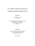
AuvTool User’s Guide
Prepared by
Junyu Zheng
H. Christopher Frey, Ph.D.
Computational Laboratory for Energy, Air and Risk
Department of Civil Engineering
North Carolina State University
Raleigh, NC
Prepared for
Office of Research and Development
U.S. Environmental Protection Agency
Research Triangle Park, NC
February 2002
i
Acknowledgments
The authors acknowledge the support of the Office of Research and Development
(ORD) of the U.S. Environmental Protection Agency, which funded this work via
contract ID-S794-NTEX.
Disclaimer
This paper has not been subject to any EPA review. Therefore, it does not
necessarily reflect the views of the Agency and no official endorsement should be
inferred. The opinions, findings, and conclusions expressed represent those of the
authors and not necessarily the EPA. Any mention of company or product names does
not constitute an endorsement by the EPA.
ii
Contents
1.0
INTRODUCTION..................................................................................................I
1.1
1.2
1.3
1.4
1.5
1.6
1.7
2.0
INSTALLING AUVTOOL .................................................................................. 6
2.1
2.2
2.3
3.0
File Menu .................................................................................................. 11
Edit Menu.................................................................................................. 13
View Menu................................................................................................ 15
Uncertainty Menu ..................................................................................... 16
Batch Mode Menu..................................................................................... 16
Window Menu .......................................................................................... 17
Help Menu ................................................................................................ 17
PROBABILITY DISTRIBUTION DEFINITIONS AND AUVTOOL
CONVENTIONS................................................................................................. 18
5.1
5.2
5.3
6.0
Starting AuvTool ........................................................................................ 8
Using AuvTool............................................................................................ 8
Exiting AuvTool ....................................................................................... 10
INTRODUCTION TO AUVTOOL MAINFRAME MENUS ........................ 11
4.1
4.2
4.3
4.4
4.5
4.6
4.7
5.0
What is Included in the Installation Package.............................................. 6
Installation................................................................................................... 6
Removing AuvTool .................................................................................... 7
GETTING STARTED .......................................................................................... 8
3.1
3.2
3.3
4.0
What is AuvTool? ....................................................................................... 1
Purpose ....................................................................................................... 1
System Requirements.................................................................................. 2
Software Tools Used in Development of AuvTool .................................... 2
Using Online Help Documentation............................................................. 3
Disclaimer of Warranties and Limitation of Liabilities.............................. 4
Copyright Notices ....................................................................................... 4
Definitions of Parametric Probability Distributions ................................. 18
Empirical Distribution .............................................................................. 19
AuvTool Conventions............................................................................... 20
DATA ENTRY, IMPORTING AND EXPORTING ....................................... 22
6.1
6.2
6.3
6.4
6.5
Input Data from the Keyboard .................................................................. 23
Loading AuvTool Data File ...................................................................... 23
Importing Data from Other Data File Formats ......................................... 24
Windows Copy and Paste ......................................................................... 25
Exporting Data from AuvTool Main Sheet .............................................. 26
i
6.6
6.7
7.0
RANDOM NUMBER GENERATORS ............................................................ 30
7.1
7.2
8.0
10.9
Showing a Graph of the Fitted Distribution for a Chosen Dataset ........... 48
Visual Comparison of Fitted Distributions with a Chosen Dataset .......... 49
Entering Uncertainty Analysis Module .................................................... 51
Variability Analysis Result Summary for All Datasets ............................ 51
Uncertainty Analysis Result Summary for All Datasets........................... 52
Saving the Current Batch Analysis Data and Property Sheet ................... 52
Loading the Existing Batch Analysis Data and Property Sheet................ 53
Automatic Batch Analysis of the Sampling Distribution ......................... 53
Data for Statistics of Interest..................................................................... 53
Exiting the Batch Analysis Module .......................................................... 56
ENTER OR LOAD DISTRIBUTIONS INFORMATION WITHOUT
ORIGINAL DATA.............................................................................................. 57
11.1
11.2
11.3
11.4
12.0
Selecting a Dataset.................................................................................... 39
Changing a Distribution Model for a Chosen Dataset .............................. 41
Changing Parameter Estimation Method .................................................. 41
Variability Analysis Results Summary for All Datasets........................... 42
Entering Uncertainty Analysis Module .................................................... 42
Exiting the Module ................................................................................... 43
CHARACTERIZATION OF VARIABILITY AND UNCERTAINTY:
BATCH ANALYSIS ........................................................................................... 44
10.1
10.2
10.3
10.4
10.5
10.6
10.7
10.8
11.0
Using the Default Random Seed............................................................... 34
Changing the Random Seed...................................................................... 35
CHARACTERIZATION OF VARIABILITY: FITTING
DISTRIBUTIONS DATASET BY DATASET ................................................ 36
9.1
9.2
9.3
9.4
9.5
9.6
10.0
Generating Random Samples Based on Parametric Distributions............ 31
Generating Random Samples Based on Empirical Distribution............... 31
RANDOM SEED SETTING.............................................................................. 34
8.1
8.2
9.0
Naming a Dataset...................................................................................... 27
Data Input Checking ................................................................................. 29
Brief Explanation of Input Specification of Columns .............................. 58
Input Distribution Information from the Keyboard .................................. 59
Loading Existing Distribution Information from a File............................ 60
Exiting the Module ................................................................................... 62
UNCERTAINTY ANALYSIS: BOOTSTRAP SIMULATION ..................... 63
12.1
12.2
12.3
Doing a Bootstrap Simulation................................................................... 65
Brief Explanation of the Graphical Displays ............................................ 66
Switching Between Graphs of Uncertainty and Probability Bands .......... 67
ii
12.4
12.5
12.6
13.0
ANALYZING THE SAMPLING DATA OF THE STATISTICS OF
INTEREST ..................................................................................................... 72
13.1
13.2
13.3
14.0
Reporting Uncertainty in the Mean and Standard Deviation.................... 84
Reporting the Summary of the Fitted Parametric Distributions to
Sampling Distribution Data for Statistics of Interest................................ 87
WORKING WITH A SHEET ........................................................................... 96
16.1
16.2
16.3
16.4
16.5
17.0
Brief Explanation of Columns in the Fitting Result Summary Table....... 81
Exporting Fitting Result Summary Table ................................................. 82
Exiting the Module ................................................................................... 82
UNCERTAINTY ANALYSIS RESULT REPORTING ................................. 84
15.1
15.2
16.0
Fitting a Distribution for a Statistic .......................................................... 76
Summarizing the Fitted Distributions for the Statistics of Interest........... 77
Exiting the Module ................................................................................... 77
VARIABILITY ANALYSIS RESULT REPORTING .................................... 79
14.1
14.2
14.3
15.0
Displaying and Saving the Bootstrap Simulation Data............................. 69
Entering the Module of Analyzing the Sampling Data of Statistics of
Interest ..................................................................................................... 70
Exiting the Module ................................................................................... 71
Copying ..................................................................................................... 96
Pasting ..................................................................................................... 96
Printing a Sheet ......................................................................................... 97
Exporting a Sheet to Tab-Delimited Text File.......................................... 98
Exporting a Sheet to a Microsoft Excel File............................................. 98
WORKING WITH A GRAPH ........................................................................ 100
17.1
17.2
17.3
17.4
17.5
Switching between the Working with Graph Popup Menu and Graph
Control Dialog Box................................................................................. 100
Editing a Graph ....................................................................................... 103
Copying a Graph to Clipboard................................................................ 116
Saving a Graph to a File.......................................................................... 116
Printing a Graph...................................................................................... 117
18.0
TROUBLESHOOTING ................................................................................... 118
19.0
REFERENCES.................................................................................................. 120
iii
1.0 INTRODUCTION
1.1
What is AuvTool?
AuvTool is a software tool for statistical analysis of variability and uncertainty
associated with fitting parametric probability distributions to data sets. It was developed
for the Office of Research and Development (ORD) of U.S. Environmental Protection
Agency, Research Triangle Park, NC.
A technical report was written for this project, with a focus on the methods and
algorithms used in the AuvTool software. The technical report contains a review of
probabilistic analysis with detailed presentation of the methods used in the AuvTool
software for fitting distributions to data, uncertainty analysis, and criteria for
automatically selecting a best distribution model in the batch analysis. The technical
report also contains a case study similar to that shown here in the User's Guide, and it
contains results of QA/AC tests. The technical report is:
Frey, H.C., J. Zheng, Y. Zhao, S. Li., Y., Zhu, Technical Documentation of the
AuvTool Software Tool for Analysis of Variability and Uncertainty, Prepared by North
Carolina State University for the U.S. Environmental Protection Agency, Research
Triangle Park, NC. February, 2002
The technical report and user’s guide are also available in the AuvTool software
package.
1.2
Purpose
The purpose of this project is to develop, evaluate, and refine a user-friendly
module for the EPA Stochastic Human Exposure Dose Simulation (SHEDS) model. The
module incorporates appropriate algorithms for assigning or fitting statistical
1
distributions to model inputs for quantifying variability in the data, and features the use
of bootstrap simulation for quantifying uncertainty in statistics for the data or fitted
distributions. However, as a stand-alone tool, AuvTool is also generally applicable to
quantifying variability and uncertainty in risk assessment, emissions estimation, and other
quantitative analysis fields.
1.3
System Requirements
The AuvTool software requires the following configurations:
•
The Intel-based computer running Windows 98/Me.
•
Any SVGA (or better) display—at least a resolution of 800x600 (or more)
pixels; a resolution of 1024x768 is recommended.
1.4
•
At least 100 Megabytes of free hard disk space.
•
At least 64 Megabytes of total memory.
Software Tools Used in Development of AuvTool
The underlying algorithms, simulation models, and Graphical User Interface
(GUI) were written in Microsoft® Visual C++ 6.0, a standard software development tool
for the Windows environment. The GUI eliminates the need to master the underlying
commands normally required in the DOS environment. Graphic Control Server 5.0A
provides graphic presentation of calculation results. Far Point Spread 3.0 provides a
spreadsheet for data entry and outputs of results.
Visual C++ runtime libraries, and the dynamic link libraries and runtime libraries
of Graphic Control Server 5.0A and Spread 3.0, are included with the AuvTool
installation package and do not need to be licensed separately.
2
1.5
Using Online Help Documentation
The online help provides an online version of this User’s Guide and of the
Technical Documentation for Analysis of Variability and Uncertainty for the AuvTool
Software via a Windows Help System.
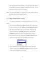
You can access the AuvTool help files by doing any one of the following when
you are running AuvTool:
•
Press F1 key.
•
Pull down the Help menu at the top of the AuvTool window, select
Help Topics.
•
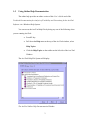
Click the Help Topics on the toolbar on the left side of the AuvTool
Window.
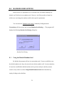
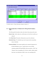
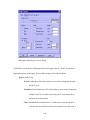
The AuvTool Help File System will display.
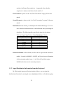
The AuvTool Online Help Documentation Window
3
1.6
Disclaimer of Warranties and Limitation of Liabilities
This report was prepared by the Computational Laboratory for Energy, Air and
Risk, located in the Department of Civil Engineering at North Carolina State University
as an account of work sponsored by the U. S. Environmental Protection Agency, Office
of Research and Development, Research Triangle Park, NC under contract No. ID-S794NTEX
This paper has not been subject to any EPA review. Therefore, it does not
necessarily reflect the views of the Agency and no official endorsement should be
inferred. The opinions, findings, and conclusions expressed represent those of the
authors and not necessarily the EPA. Any mention of company or product names does
not constitute an endorsement by the EPA.
NEITHER ANY MEMBER OF EPA, ANY COSPONSOR, THE ORGANIZATION(S) NAMED
BELOW, NOR ANY PERSON ACTING ON BEHALF OF THEM: (A) MAKES ANY WARRANTY OR
REPRESENTATION WHATSOEVER, EXPRESS OR IMPLIED, (I) WITH RESPECT TO THE USE OF
ANY INFORMATION, APPARATUS, METHOD, PROCESS, OR SIMILAR ITEM DISCLOSED IN
THIS REPORT, INCLUDING MERCHANTABILITY AND FITNESS FOR A PARTICULAR
PURPOSE, OR (II) THAT SUCH USE DOES NOT INFRINGE ON OR INTERFERE WITH
PRIVATELY OWNED RIGHTS, INCLUDING ANY PARTY'S INTELLECTUAL PROPERTY, OR (III)
THAT THIS REPORT IS SUITABLE TO ANY PARTICULAR USER'S CIRCUMSTANCE; OR (B)
ASSUMES RESPONSIBILITY FOR ANY DAMAGES OR OTHER LIABILITY WHATSOEVER
(INCLUDING ANY CONSEQUENTIAL DAMAGES, EVEN IF EPA OR ANY EPA
REPRESENTATIVE HAS BEEN ADVISED OF THE POSSIBILITY OF SUCH DAMAGES)
RESULTING FROM YOUR SELECTION OR USE OF THIS REPORT OR ANY INFORMATION,
APPARATUS, METHOD, PROCESS, OR SIMILAR ITEM DISCLOSED IN THIS REPORT.
1.7
Copyright Notices
Graphics Server 5.0A, Copyright © 1996, Bits Per Second Ltd. and Pinnacle
Publishing, Inc. All Rights Reserved.
Spread 3.0, Copyright © 1998, FarPoint Technologies, Inc, All Rights Reserved.
Microsoft Visual C++ 6.0, Copyright © 1999, Microsoft Corporation. All Rights
Reserved.
4
Analysis of Uncertainty and Variability Tool (AuvTool) and Interface (AuvTool)
1.0, Copyright © 2001, North Carolina State University. All Rights Reserved.
Graphics Server is a trademark of Bits Per Second Ltd.
Microsoft is a registered trademark; Windows, Windows 95, and Visual C++ are
trademarks of Microsoft Corporation.
SpreadTM is a trademark of FarPoint Technologies, Inc.
5
2.0 INSTALLING AuvTool
2.1
What is Included in the Installation Package
The AuvTool installation package contains the following items:
•
Installation CD-ROM: All the software is on the CD-ROM in compressed
form. An installation program included on the CD-ROM will install the
necessary files automatically. See "Installation" below for instructions.
•
Two pieces of documentation: User’s Guide, and Technical Report. These
are included as Adobe PDF documents on the installation disk, and can be
opened or copied to another disk.
2.2
Installation
To install the AuvTool program, you must use the installation program,
SETUP.EXE, provided on the installation CD-ROM. Simply copying the contents of the
CD-ROM to your hard drive will not work because the programs are on the CD-ROM in
compressed form. Program files must be decompressed and installed in the appropriate
directories to run properly. Copying the contents of the distribution CD-ROM to a local
hard drive can speed up the installation process.
To run the Setup Program
1. Place the A CD-ROM in your CD-ROM drive;
2. Click the Start button;
3. Choose Run… from the Start menu; and
6
4. Type “X:\ XXX\” SETUP.EXE” where “X:\ ” is the drive and directory to
which you copied the installation files.
The Installation Program will begin. Follow the instructions on the screen.
You also can install AuvTool as follows:
1. Place the AuvTool CD-ROM in the CD-ROM drive;
2. Double-click the My Computer icon on the desktop;
3. Double-click the CD-ROM drive in the My Computer window; and
4. Double-click the “SETUP.EXE” on the CD-ROM.
The Installation Program will begin. Follow the instructions on the screen.
2.3
Removing AuvTool
To remove the AuvTool software completely, use the uninstall feature of the
Windows 98/Me “Add/Remove Software” in the Control Panel.
Note: Do not delete the files in the AuvTool directory. Although you may disable
the program, it will not completely uninstall the program, because there are files
elsewhere on your system that should also be cleaned up.
To Run the Uninstall Program
1. Click the Start button.
2. Choose Settings, and then Control Panel.
3. Double-click Add/Remove Programs in the Control Panel folder.
4. Highlight AuvTool on the list of installed software.
5. Click the Add/Remove… button.
Follow the instructions on the screen.
7
3.0 GETTING STARTED
3.1
Starting AuvTool
A program group called AuvTool is created when the software is installed.
“AuvTool” will be displayed in the Programs group in the Start Menu. To start the
AuvTool program, click on the AuvTool program icon in the Start Menu.
The program will launch, and a picture will be displayed. The display is as
follows:
The picture will disappear in 2 seconds, after which the AuvTool mainframe window will
appear and the program will be ready for use.
3.2
Using AuvTool
These are the steps or options involved in running AuvTool:
•
Start AuvTool (See “Getting Started ” on page 8).
•
Data Entry, Importing and Exporting (see page 22).
•
Random Number Generators (see page 30 ).
•
Random Seed Setting (see page 34).
8
AuvTool Mainframe and Main Sheet
•
Characterization of Variability: Fitting Distributions Dataset by Dataset (see
page 36).
•
Characterization of Variability and Uncertainty: Fitting Distributions by
Batch Analysis (see page 44).
•
Load Distribution Information without Original Data (see page 57).
•
Uncertainty Analysis: Bootstrap Simulation (see page 63).
•
Fitting Distributions to the Sampling Data of the Statistics of Interests (see
page 72).
•
Variability Analysis Result Reporting (see page 79).
•
Uncertainty Analysis Result Reporting (see page 84).
9
3.3
•
Working with a Graph (if desired) (see “ Working with Graph ” on page 100).
•
Working with a Sheet (if desired) (see “ Working with Sheet ” on page 96).
•
Exit AuvTool (see “ Exiting AuvTool ” on this page).
Exiting AuvTool
To exit AuvTool, do one of the following:
•
Pull down the File pull down menu or press Alt-F and select Exit;
•
Click the Close button (x) in the upper right hand corner of the AuvTool
mainframe window; or
•
Press Alt-F4.
10
4.0 INTRODUCTION TO AUVTOOL MAINFRAME
MENUS
In this section, we will give a brief introduction to the AuvTool Mainframe Menu
Commands.
4.1
File Menu
File | New (Ctrl+N)
This command creates a new data sheet window with the default name
“AuvToo1.” AuvTool prompts you to name an "AuvTool" file when you save it.
File | Open (Ctrl+O)
This displays a standard Open File dialog box with the default file search
extension “ *.ss3.” You can use this command to open an existing data file saved by
AuvTool.
The following options allow you to specify which file to open:
File Name
Type or select the filename you want to open. This box lists files with the
extension you select in the List Files of Type box.
List Files of Type
Select the type of file you want to open: “*.ss3”
Drives
Select the drive in which AuvTool stores the file that you want to open.
Directories
Select the directory in which AuvTool stores the file that you want to open.
Once you have typed a proper filename in the File Name edit box, choose the OK
to open the file you specified.
11
Note: Before you open an existing file, you need to first open an empty sheet by
clicking the File | New command.
File | Close
This command lets you close the current active datasheet.
File | Import Excel…
The File | Import Excel menu item displays an Open File dialog box with the
default file search extension “*.xls.” You can use this command to open an existing
Microsoft Excel TM 97 file format data. You should specify a file to open by clicking on
it or inputting the file name.
File | Import Tab-Delimited …
The File | Import Tab-Delimited menu item displays an Open File dialog box
with the default file search extension “*.txt.” You can use this command to open a data
file which is saved with with tab delimiters between numbers. You should specify a file
to import by clicking on it or inputting the file name.
File | Save (Ctrl+S)
This command saves the data in the active data sheet to disk.
File | Save As
This command lets you save the active data sheet to a different name, in a
different directory or on a different drive. When you choose this command, the Save File
As dialog box is displayed. This Save File As dialog box is similar to the Open Sheet
dialog box. You can enter the new name, optionally with drive and directory, and click
the Save button to accept the dialog box input.
12
File | Print Preview
This command lets you see an on-screen preview of how the data sheet will
appear on a printed paper.
File | Print ...
This command lets you print the active sheet data. Please make sure that a printer
is properly connected to your computer and that it is turned on before you choose this
command.
File | Printer Setup
This command lets you select a target printer for data sheet output. This
command displays the standard Windows Print Setup dialog box that you can use to set
up your printer.
File | Exit
This command exits AuvTool, removes it from memory, and returns you to the
Windows environment. If you have made any changes that you have not saved, AuvTool
asks you if you want to save them before exiting.
4.2
Edit Menu
The menu commands listed in the Edit Menu will apply to the AuvTool Main
Sheet.
Edit | Cut (Ctrl+X)
The Edit | Cut command removes the selected data block from your data sheet and
places the data in the Clipboard. The removed data cells are filled with blank cells. You
can paste that data into any other data sheet or somewhere else by choosing the Edit |
13
Paste command. The data remains in the Clipboard so that you can paste the same data
many times.
Edit | Copy (Ctrl+C)
The Edit | Copy command places the selected data in the Clipboardand leaves the
selected data intact. You can then paste that data into any other data sheet or any other
editors by choosing Edit | Paste command.
Edit | Paste (Ctrl+P)
The Edit | Paste command puts data from the Clipboard into the current data sheet
at the cursor position. This action depends on what you have in the Clipboard. If the
data in the Clipboard contains columns (rows), then it will paste data in columns starting
at the column (row) which contains the cursor cell; if the data in the Clipboard contains
only a block of data cells, then the paste action will put the data to the sheet starting at the
current cursor cell. The paste action overwrites data in the data sheet. It does not insert
data into the data sheet.
Edit | Delete
The Edit | Delete command works like the Edit | Clear command. It removes the
selected data from the data sheet but does not place it into the Clipboard. This command
also shifts the data sheet so that there are no blank cells.
Edit | Insert
This menu item has a pop-up menu (or a sub-menu) which contains two
commands. These commands let you insert one blank column and one blank row.
Column
This command inserts a blank column at the current cursor column position.
14
Row
This command inserts a blank row at the current cursor row position.
Edit | Delete
The Edit | Delete command works like the Edit | Clear command. It removes the
selected data from the data sheet but does not place it into the Clipboard. This menu item
has also a pop-up menu (or a sub-menu) which contains two commands. These
commands let you delete one blank column and one blank row.
Column
This command deletes a blank column at the current cursor column position.
Row
This command deletes a blank row at the current cursor row position.
This command also shifts the data sheet so that there are no blank cells
Edit | Clear
The Edit | Clear command removes the selected data from the data sheet but does
not place it into the Clipboard. The removed data cells are filled with blank cells. This
means that you can not paste the data as you could if you had chosen Cut or Copy
commands.
4.3
View Menu
View | Toolbar
This command controls the display of toolbar within the main window frame. If
checked, it will display the toolbar. If not checked, the toolbar will not be displayed.
View | Status Bar
This command controls the display of status bar within the main window frame.
If checked, it will display the status bar. If not checked, the status bar will not be
displayed.
15
4.4
Uncertainty Menu
Uncertainty | Random Seed Setting…
This command will popup a dialog which allows users to set the random setting.
See “Random Seed Setting ” on page 34 for more details.
Uncertainty | Random Generator…
This command will popup a dialog which allows users to generate random
numbers from normal, lognormal, gamma, beta, Weibull, uniform, symmetric triangle
and empirical distributions. For more details, see “Random Number Generator” on page
30.
Uncertainty | Single Distributions…
This command will popup a dialog box which allows users to estimate parameters
for normal, lognormal, gamma, beta, Weibull, uniform, symmetric triangle distributions
single dataset by single dataset. For more details, see “Characterization of Variability:
Fitting Distribution Dataset by Dataset” on page 36.
4.5
Batch Mode Menu
Batch Mode | Load Distributions…
This command will popup a dialog which allows users to load or enter existing
distribution information that users have for batch uncertainty analysis. For more details,
see “ Enter or Load Distribution Information ”on page 57.
Batch Mode | Batch Analysis…
This command will popup a dialog which allows users to do batch variability and
uncertainty analysis for their datasets. It includes: parameter estimation, bootstrap
16
simulation, automatic best distribution selection and so on. For more details, see
“Characterization of Variability and Uncertainty: Batch Analysis” on page 44.
4.6
Window Menu
The Window menu contains window management commands. At the bottom of
this menu, all currently opened child window are listed.
Window | Cascade
This command rearranges all open sheet/plot windows in overlapping layers. The
title of each window is revealed so that you can see the name of the sheet/plot it contains.
Window | Tile
This command displays all open sheet/plot windows without overlapping them.
When possible, the windows are all given equal room on the screen.
Window | Arrange Icon
After several open sheet/plot windows are minimized as icons in the main
window, this command can quickly place the icons in neat rows along the bottom of the
screen.
4.7
Help Menu
Help | Help Topics
This command will pop up AuvTool online help documentation dialog box.
Help | About AuvTool
This command will display the version information about AuvTool.
17
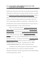
5.0 PROBABILITY DISTRIBUTION DEFINITIONS AND
AUVTOOL CONVENTIONS
In this section, definitions of probability distributions used in the AuvTool are
presented. The conventions used in the AuvTool are also introduced.
5.1
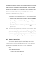
Definitions of Parametric Probability Distributions
Commonly used parametric distributions used in variability and uncertainty
analysis include normal, lognormal, Weibull, gamma, beta, uniform and triangle
distributions. Table 5-1 lists the definitions for the seven common parametric
distributions included in AuvTool.
Table 5-1. Definitions of Probability Distribution Density Function for Parametric
Distribution in Included in AuvTool
Name of
Distribution
Normal
Lognormal
Probability Density Function (PDF)
f (x) =
f (x) =
(
− x −µ
1
2πσ
2
2σ
e
− (ln x −µ ln x )2
1
x 2πσ ln x
)2
2
2
2σ2
e
x α −1 (1 − x )
Β (α , β)
(0 < x < ∞ )
β −1
Beta
Gamma
Weibull
Uniform
Symmetric
Triangle
f (x) =
β − α x β−1e − x β
Γ(α )
c
f ( x ) = ( x k ) c −1 exp(−( x k ) c )
k
1
f (x) =
b−a
b− | x − a |
f (x) =
b2
f (x) =
18
( 0 ≤ x ≤ 1)
(0 ≤ x < ∞ )
(0 ≤ x < ∞ )
(a ≤ x ≤ b)
( a − b ≤ x ≤ a + b)
In the Table 5-1, for the normal distribution, µ is the arithmetic mean, and σ is the
arithmetic standard deviation. For the lognormal distribution µlnx is the mean of ln(x),
and σlnx is the standard deviation of ln(x). In the beta distribution, α and β are shape
parameters, and B(α, β) is the beta function. For the gamma distribution, α is the shape
parameter, β is the scale parameter, and Г(·) is the gamma function. For the Weibull
distribution, k is the scale parameter, and c is the shape parameter. For the uniform
distribution, a and b are the smallest and largest possible values. For the symmetric
triangle distributions, a and b determine the range that a variable can vary.
5.2
Empirical Distribution
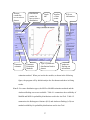
An empirical distribution can be defined as a discrete distribution, F, that gives
equal probability, 1/n, to each value xi in the dataset, x (Efron, 1979). The CDF for this
function is therefore a step function of original data set, x, where each value xi is assigned
a cumulative probability of i/n for i= {1,2,…n}. An example of an empirical distribution
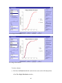
Cumulative Probability
represented a step function for a data set with n=10 is provided in Figure 5-1.
1
0.8
0.6
0.4
0.2
0
0
2
4
6
Example Data
Figure 5-1. An example of an Empirical Distribution Represented a Step
Function
19
8
Table 5-2. Conventions for 1st Parameter and 2nd Parameter Terms Used in AuvTool
1st Parameter
2nd Parameter
Distribution Name
Normal
Mean, µ
Standard Deviation, σ
Lognormal
Standard Deviation of ln(x), σlnx
Mean of ln(x), µlnx
Beta
Shape, α
Shape, β
Gamma
Scale, α
Shape, β
Weibull
Scale, k
Shape, c
Uniform
Minimum, a
Maximum, b
Symmetric Triangle
a
b
(Please refer to the Technical Documentation for detailed definitions of these
distributions and other relevant information)
5.3
AuvTool Conventions
1st parameter and 2nd parameter
Each parametric distribution contained in this version of AuvTool is described by
two parameters. In some modules, we use the 1st parameter and 2nd parameter to
represent the two parameters. The specific interpretation of each parameter differs for
different types of parametric distributions is presented in Table 5-2.
Note: The user does not have to be familiar with the mathematical formulation of the
parametric probability distribution models or with the interpretation or the values
of the parameters in order to use this program.
Introduction to the Example Used in the User’s Guide
In the User’s Guide, we use an example study to help describe the use of the
AuvTool. The example datasets shown in the all pictures in the Guide come from the
example study. In the example study, there are five datasets with original data, which are
named as “ Dataset 1”, “ Dataset 2”, “ Dataset 3”, “ Dataset 4”, and “ Dataset 5”
20
respectively; and three datasets without original data, which are named as “NoDataName
1”, “NoDataName 2”and “NoDataName 3”, respectively. These datasets are included in
two files, which are called “ExampleWithData.ss3” and “ExampleWithoutData.ss3”,
repectively. The two files are contained in the installation package of AuvTool. During
the process of installing AuvTool, the setup program will automatically copy the two files
to the working directory of AuvTool. You can find these two files in this directory.
21
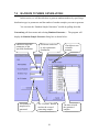
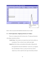
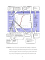
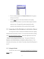
6.0 DATA ENTRY, IMPORTING AND EXPORTING
In this section, you will learn how to enter data in the AuvTool data Main Sheet
for variability and uncertainty analysis and how to import or export data through
AuvTool.
Before you can do any analysis using AuvTool, you must provide data to the
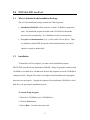
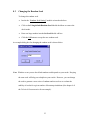
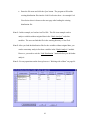
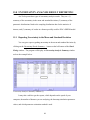
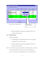
Main Sheet in the AuvTool mainframe window as shown in the following:
Edit Box to show
where the current
cursor is
“Name
Dataset” button
“Name Dataset”
Edit Box
Check Box to
specify whether
the first row is a
title row
AuvTool Main
Sheet
AuvTool Main
Frame
AuvTool Main Frame and Main Sheet
22
After you start AuvTool, the program will provide you with a blank sheet as
shown above. There are four ways to enter data. You can enter data by keyboard, load
data from an existing AuvTool disk file, import data from other file formats or use the
Window copy and paste command located Edit menu in the AuvTool Main Frame to
enter data.
6.1
Input Data from the Keyboard
You can enter data by moving the cursor (highlighted cell) to a cell and then
typing a number. Press <Enter> key to accept the input and the cursor will automatically
move down one row. Repeat this step to enter the remaining data in the column. If you
want to change the data in a cell, just move the cursor to the cell, type another value and
press <Enter>.
Tip: You can also use arrow key to accept the value in the current active cell and move
the active cell to the next cell pointed by the arrow.
Note: In AuvTool, it is specified that each column in the Main Sheet represents one
dataset. If you have multiple datasets, you have to enter the different datasets into
different columns. You must name each dataset. You can refer to the “Naming a
Dataset” section on page section 27 for how to name a dataset.
6.2
Loading AuvTool Data File
AuvTool has its own data file format with an extension of “.ss3” or “.SS3”. It is
in a binary format.
To open an existing AuvTool data sheet file:
23
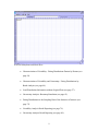
•
Pull down the File pull down menu (or press Alt-F) and select Open, or just
click the Open icon on the tool bar. The program will display an Open file
dialog box as shown below:
•
Find the file name that you would like to open. Click the Open button in the
Open dialog box.
The AuvTool main sheet will load your data. Now you can use any features that
AuvTool provides.
6.3
Importing Data from Other Data File Formats
AuvTool can also exchange data with many popular data file formats such as
Microsoft Excel TM files (XLS) and Tab-Delimited files provided by any text editor.
Since the AuvTool data sheet can only handle numerical value and text string (only for
the first row, when used as a title of a dataset) when you import data into AuvTool, make
24
sure the data file contains only numerical values except for text strings that are contained
in the first row or the column headers. Otherwise, the program will provide a warning
message box to show you that the text in a particular cell is not a valid numerical value.
You must correct all the mistakes before you can do further analysis. For more
information, see “Data Input Checking” on page 31.
To import data to AuvTool from Microsoft Excel TM files or Tab-Delimited files:
•
Pull down the File pull down menu (or press Alt-F) and select File| Import
Excel… or File | Import Tab-Delimited File; the program will display an
Open file dialog box.
•
Find the file name that you would like to open. Click the Open button in the
Open dialog box.
Note: AuvTool can only support importing a 97 Microsoft Excel TM file format. Make
sure that your datasheet files are saved in the form of 97 Microsoft Excel TM file.
For some rare cases, if you find that you cannot import an Excel TM data file, you
also can use the following Window Copy and Paste features to import your data.
6.4
Windows Copy and Paste
Data can also be imported or exported by using Windows Copy and Paste
command which are often listed in the Edit menu between the Windows application
programs based on a spreedsheet such as Excel TM, Access TM, and AuvTool.
Copy
To copy data from a spreadsheet:
1. Select the cells that you want to copy.
25
2. Do any one of the following:
•
Pull down the Edit menu and select the Copy.
•
Click the Copy button on the toolbar on the left side of the AuvTool.
•
Press Ctrl-C
Paste
To paste data from a spreadsheet:
1. Select the cells that you want to paste data into.
2. Do any one of the following:
6.5
•
Pull down the Edit menu and select the Paste.
•
Click the Paste button on the toolbar on the left side of the AuvTool.
•
Press Ctrl-V
Exporting Data from AuvTool Main Sheet
AuvTool provides features to save the current main data sheet or to export the
current datasheet to other file formats such as Microsoft Excel TM or tab-delimited text.
AuvTool also can make use of Window Copy and Paste features introduced above to
export data to other application programs.
To save the current data sheet:
•
Pull down the File pull down menu (or press Alt-F) and select Save, or Save
as, or just click the Save icon on the tool bar. The program will display an
Save as file dialog box.
•
Enter a filename with an extension of “.ss3”. Click the Save button in the
Save as dialog box.
To export the current data sheet to a Microsoft Excel TM file format:
26
•
Pull down the File pull down menu (or press Alt-F) and select Export
Excel…, The program will display an Save as file dialog box with the initial
file type of “.xls”.
•
Enter a filename with an extension of “.xls”. Click the Save button in the
Save as dialog box.
Note: In order to make sure that your data will not be lost, we recommend that you also
save your current datasheets as an AuvTool file format when you export your data
to a Microsoft Excel TM file. Please also refer to the “Troubleshooting ” section
on page 118.
To export the current data sheet to a Tab-Delimited Text file format:
•
Pull down the File pull down menu (or press Alt-F) and select Export TabDelimited…, The program will display an Save as file dialog box with the
initial file type of “.txt”.
•
Enter a filename with an extension of “.txt”. Click the Save button in the
Save as dialog box.
Note: When you save a file, you can save the file to any other directory you want. Just
select the drive letter and the directory you want to save to in the Directories box.
You can also save the file to a floppy disk. In order to do that, just change the
drive to the drive letter of your disk.
6.6
Naming a Dataset
AuvTool requires that user must name each dataset inside the AuvTool main
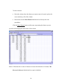
sheet. As introduced above, each column stands for a dataset. The figure shown on the
next page displays how the AuvTool “Name Dataset” feature works.
27
To name a dataset:
•
Select the column where the dataset you want to name is located, or place the
cursor inside any cells of the column.
•
Enter names into the Name Dataset labeled edit box directly above the
spreadsheet.
Click the Name Dataset button, and the name representing the dataset you just
specified will be displayed in the header of the column.
Note 1: When the titles or name of datasets are located in the headers of columns, The
first row is title row labeled check box must be disabled.
28
Note 2: AuvTool does not require that the names representing different datasets in the
same sheet be unique. However, for your convenience in identifying different
datasets, we recommend that you use different names for different data sets.
Note 3: When the program imports data from other application programs such as from
the Excel TM, sometimes, the name or titles of datasets are located in the first row.
In this situation, The first row is title row labeled check box must be enabled by
clicking on it. This check box is located immediately to the right of the text box
for Name Dataset entry. If there are no names or titles for the imported datasets,
users have to name them as introduced above.
Note 4: For any AuvTool sheet files, all of the names of all datasets within the same file
are located at either the column header or the first row.
6.7
Data Input Checking
AuvTool has a feature to logically check the users’ data input. AuvTool assumes
that the data within any cells are valid numerical values except for the first row when the
The first row is title row labeled check box is enabled. The feature will be invoked
when users try to make further analysis. If there exists any invalid non-numerical values
such as a text string in a particular cell, the program will pop up a message box showing
“not a valid numerical value at row n, column m.” Users must correct all the exceptions
before they can do further data analysis.
29
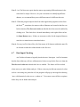
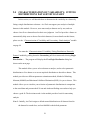
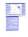
7.0 RANDOM NUMBER GENERATORS
In this section, we will describe how to generate random numbers by specifying a
distribution type, its parameters and the number of random samples you want to generate.
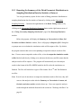
You can enter the “Random Sample Generators” module by pulling down the
Uncertainty pull down menu and selecting Random Generator…. The program will
display the Random Sample Generator dialog box as shown below:
Edit box to enter the
parameters of the
specified distribution
The number of
samples to be
generated
Pull down combo box
to select parametric
distribution
The “Generate” Button
invokes the event of
generating samples
30
Check box to use
scientific
notation
The sheet to hold
the generated
samples
In the above dialog box, we have specified a normal distribution with mean of 1.0
and standard deviation of 0.5, and generated 100 random samples from the distribution.
The results are displayed in the spreadsheet on the right side.
Note 1: For “First parameter” and “Second Parameter” definitions, please see the section
of “ Probability Distribution Definitions and AuvTool Conventions ”on opage 20.
Note 2: For information on how to save or export the sampling results, please see
“Working with a Sheet” on page 96.
7.1
Generating Random Samples Based on Parametric Distributions
To generate random samples:
•
Specify the distribution type, enter the first and second parameters, and
specify the number of samples.
•
Click Generate button, the sampling results will be displayed in the first
column of the sheet.
Note 1: If you find that there are not sufficient significant figures in reporting results for
small numbers, check the Scientific Notation labeled checkbox by clicking on it.
The program will report the results in scientific format.
7.2
Generating Random Samples Based on Empirical Distribution
AuvTool has a feature to generate random samples based on an empirical
distribution.
To generate random samples based on an empirical distribution:
•
Pull down the Distribution Type combo box in the Random Sample
Generator dialog box, and select “Empirical Distribution.” The program will
31
prompt you to enter your dataset into the first column of the data sheet. The
Random Sample Generator dialog box will become:
•
Enter your dataset into the first column of the sheet labeled “A” as shown in
the above figure.
•
Click the Generate button. The sampling results will be displayed in the
second column of the sheet labeled “B” as shown on the next page.
Note: If you find that there are not sufficient significant figures in reporting
results for small numbers, check the Scientific Notation labeled checkbox by clicking on
it. The program will report the results in scientific format.
32
33
8.0 RANDOM SEED SETTING
In this section, we explain how to set a random seed for random sampling. By
default, AuvTool has its own random seed. However, AuvTool provides a feature by
which users can change the random seed for their special requirements.
You can enter the “Random Seed Setting” module by Pulling down the
Uncertainty pull down menu and selecting Random Seed Setting…. The program will
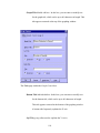
display the following Random Seed Setting dialog box:
Random Seed Setting
8.1
Using the Default Random Seed
By default, the program will use its own random seed. If users would like to use
the default random seed, they do not need to invoke the module at all. In some situations,
if users have modified the default random seed in previous analysis, and they want to
restore it; they need to reset the Using Default Random Seed labeled checkbox by
simply clicking on the checkbox.
34
8.2
Changing the Random Seed
To change the random seed:
•
Invoke the “Random Seed Setting” module as introduced above.
•
Click on the Using default Random Seed labeled checkbox to remove the
check mode.
•
Enter one large number into the Set Seed labeled edit box.
•
Click the OK button to accept the new random seed.
An example dialog box for changing the random seed is shown below:
Note: Whether or not you use the default random seed depends on your needs. Keeping
the same seed will help you to duplicate your results. However, you can change
the seed to generate a new series of random numbers such as to evaluate the
stability of results for a given number of bootstrap simulations (See chapter 4 of
the Technical Documentation for an example).
35
9.0 CHARACTERIZATION OF VARIABILITY: FITTING
DISTRIBUTIONS DATASET BY DATASET
In this section, we will describe how to characterize the variability in a dataset by
fitting a single distribution to a dataset. AuvTool can support your analysis of multiple
datasets in this module. However, users must analyze datasets one by one, and can
choose a best fit to a dataset based on their own judgment. AuvTool provides a feature to
automatically help users to choose fits to their datasets; for more details on this feature,
please see the “Characterization of Variability and Uncertainty: Batch Analysis” module
on page 44.
You enter the “Characterization of Variability: Fitting Distributions Dataset by
Dataset” module by pulling down the Uncertainty pull down menu and selecting Single
Distribution…. The program will display the Fit a Single Distribution dialog box
shown on the next page.
This module allows you to select a dataset to analyze, and to select parametric
distributions to fit a dataset or to use an empirical distribution to describe a dataset. This
module provides two different parameter estimation methods, Method of Matching
Moment (MoMM) and Maximum Likelihood Estimation (MLE), for you to choose. This
module allows you to visualize your selection of parametric distributions in comparison
to the actual data and presents the K-S test and Anderson Darling test results to help you
choose a good fit. The decisions made via the module provide a basis for uncertainty
analysis.
Note 1: Initially, AuvTool assigns a default normal distribution to all datasets listed in
the dataset list combo box, and sets MoMM as the default parameter
36
Dataset
combo list
box to select a
dataset
Parameter
estimates
Distribution
combo list
box to select a
distribution
Parameter
Estimation
Methods
Graph
title
Number
of data
points
Type of parametric
distribution fitted to
dataset
K-S test
information
AndersonDarling test
information
estimation method. When you invoke the module, as shown in the following
figure, the program will by default analyze the first dataset and show its fitting
results.
Note 2: For some distribution types, the MLE or MoMM estimation methods and the
Anderson-Darling test are not available. Table 9-1 summarizes the availability of
MoMM and MLE for probability distributions used in the AuvTool. Table 9-2
summarizes the Kolmogorov-Smirnov (K-S) and Anderson-Darling (A-D) test
method availability for probability distributions used in AuvTool.
37
Table 9-1. Parameter Estimation Method Availability for Probability Distributions
Distribution
MoMM
(MLE)
Comments
Types
Normal
Analytic solution for MLE
√
√
Lognormal
Analytic solution for MLE
√
√
Beta
Optimal Solution for MLE
√
√
Gamma
Optimal Solution for MLE
√
√
Weibull
Optimal Solution for MLE
▲
√
Uniform
N/A
√
Symmetric
Optimal Solution for MLE
√
√
Triangle
Note: √: The method is available for the given distribution.
▲: The plotting method is used instead of MOMM for Weibull distribution
N/A: The method is not available in this case
Table 9-2. Goodness-of-fit Test Method Availability for Probability Distributions
Distribution
Kolmogorov-Siminov
Anderson-Darling Test
Types
Test
Normal
√
√
Lognormal
√
√
Beta
√
Gamma
√
√
Weibull
√
√
Uniform
√
Triangle
√
Note: √: The test is available for the given distribution.
Note 3: For some datasets, some distributions cannot be used to fit them. For example,
lognormal, gamma and Weibull distributions cannot be used to describe datasets
in which there are some negative values, and a beta distribution cannot represent a
dataset in which some values are outside of the range between 0 and 1. If such
situations occur, AuvTool will provide a message box to suggest that users choose
other distributions. However, in some cases, the normal distribution might be
chosen by a user or the automatic batch fit process to represent a dataset that must
be non-negative. Because the program does not know which datasets must be
38
non-negative, it is the user’s responsibility to make sure that the normal
distribution is not used inappropriately.
Note 4: The data and parametric distributions are shown in terms of cumulative
probability (on the Y-axis) versus values of the dataset (or a variable) (on the Xaxis). Cumulative probability is the probability that a randomly selected sample
within the variable will have a value less than or equal to the associated value of
the variable on the X-axis.
Note 5: On graphs that depict the origin of the X-axis, a spurious symbol appears at a
cumulative probability of zero and an x-value of zero. This is not an actual data
point; it is an artifact of the graphics routine used at this time.
Note 6: Each graph depicts both the available data set, shown as triangular data symbols,
and the parametric distribution, shown as a smooth line. The legend of the graph
indicates the number of data points available and the type of parametric
distribution currently selected. The graphical display allows you to visualize both
the data and the parametric distribution. Some disagreement will typically be
evident when comparing the distribution to the data. The program gives you a
capability to select from several alternative parametric distributions in most cases.
You can choose the one that has the best fit in your opinion.
Note 7: If you want to edit a graph, save a graph as a file, or print a graph out, please see
the section “Working with a Graph” on page 100.
9.1
Selecting a Dataset
If you have multiple datasets to analyze, you should select a dataset as a current
dataset and then analyze it as shown below.
39
Fit a Single Distribution
Fit a Single Distribution
To select a dataset:
•
Pull down the Data Sets labeled combo list box menu on the left hand position
of the Fit a Single Distribution window;
40
•
Click the dataset name you want to choose; and
•
The graph will be updated automatically and the estimation results will also be
updated.
9.2
Changing a Distribution Model for a Chosen Dataset
If you do not think that the current parametric probability distribution for the
dataset you are analyzing is a good one, you can change it.
To make a change of parametric distribution:
•
Pull down the Distribution Type combo list box menu on the left side of the Fit
a Single Distribution window;
•
Click the distribution type you want to choose; and
•
The graph will be updated automatically and the estimation results will also be
updated.
9.3
Changing Parameter Estimation Method
AuvTool provides options for users to choose one of two parameter estimation
methods. The AuvTool sets MoMM as the default estimation method. However, users
can freely choose either MoMM or MLE. For more information on the two parameter
estimation methods, please see “Parameter Estimation of Parametric Probability
Distributions” in the Technical Documentation.
To make a change of parameter estimation method:
•
Click on the radio box of the method you want to choose.
•
Click on the Go button on the left side of the Fit a Single Distribution
window.
41
•
The graph will be updated automatically and the estimation results will also be
updated.
Note: For the uniform distribution, MLE is not available. In this situation, the MLE
radio box is disabled. For the empirical distribution, neither MLE nor MoMM are
applicable, so both of the radio boxes are disabled in this case.
9.4
Variability Analysis Results Summary for All Datasets
After you have reviewed or modified the selection of parametric probability
distributions and parameter estimation method, you can obtain a summary of the
distributions, parameters of distributions associated with each dataset, parameter
estimation method used and statistical test results. To do this:
•
Click the Fitting Result Summary button on the Fit a Single Distribution
window.
•
The program will display a popup Fitting Result Summary dialog box. More
information can be found on “Variability Analysis Result Reporting” on page
79.
9.5
Entering Uncertainty Analysis Module
The decisions or choices of distribution types and parameter estimation methods
you made in the “Characterization of Variability: Fitting Distributions Dataset by
Dataset” module will provide a basis for uncertainty analysis using bootstrap simulation.
To enter the uncertainty analysis module:
•
Click the Bootstrap button on the Fit a Single Distribution window.
42
•
The program will display a popup Bootstrap Simulation dialog box with three
tab-pages. More information on uncertainty analysis can be found on
“Uncertainty Analysis: Bootstrap Simulation” on page 63.
9.6
Exiting the Module
You have two ways to exit the module:
•
The OK button or Cancel button on the Fit a Single Distribution window.
•
Click the Close icon of the right corner of the Fit a Single Distribution
window.
43
10.0 CHARACTERIZATION OF VARIABILITY AND
UNCERTAINTY: BATCH ANALYSIS
This section describes the “Characterization of Variability: Batch Analysis”
module in AuvTool used to quantify variability for multiple datasets. This module helps
users automatically analyze multiple datasets. However, it also allows users to select a
parameter estimation method and a fit to a dataset based on their own judgment.
Therefore, it provides a flexible way for users to do variability analysis.
The arithmetic
mean of each
dataset
The arithmetic
standard deviation
of each dataset
Batch Fitting (1)
Batch analysis
data and
property sheet
“Auto” is not a
distribution type. It is
an option
This Setting group is used to
automatically batch-analyze
the sampling distribution for
the statistics of interest
You can enter the module by pulling down the Batch Mode pull down menu in
the AuvTool Mainframe window and selecting Batch Analysis…. The program will
display the above Batch Fitting dialog box.
44
These datasets have original
data, the information is from
AuvTool Main Sheet
Click here to graphically
show the goodness of the
fit to the selected dataset
The number of
bootstrap
samples
Batch Fitting (2)
Those variables do not
have original data. The
information is from the
“Link Distribution”
module
If checked, the original
data is available for this
variable
The “Batch Analysis” module is more powerful than the “Fitting Distribution
Dataset by Dataset” module previously introduced. It includes all features implemented
in the “Fitting Distribution Dataset by Dataset” module, but also it provides the following
capabilities of automatic batch analysis; and visual comparison of different distribution
types fitted to a dataset; and uncertainty analysis for known distributions without the
original datasets. Users can finish their analyses of variability and uncertainty for
multiple datasets without having to make any choices. The program will automatically
help users to choose best fits and to do uncertainty analysis. For the criteria of selecting
45
a best fit to a dataset, please refer to “Criteria for Automatically Seeking a Best
Distribution Model in the Batch Mode Analysis” in the Technical Documentation.
The “Batch Analysis” module can support uncertainty analysis without original
datasets if users can provide necessary distribution information. Users cannot directly
introduce the information into the batch analysis data and property sheet, which must be
done via the “Link Distribution” module. For more details on how to introduce the
known distribution information into the “Batch Analysis” module, please see the module
of “Load Distributions Information” on page 57.
WARNING: The user of AuvTool is cautioned that the availability of a batch mode
technique for choosing a distribution based upon the K-S test is not a substitute
for the use of judgment. The K-S test is based upon a specific criterion which
may or may not be important to a particular analyst or decision maker in the
context of a specific problem. The K-S test does not screen for results that may
be physically implausible, such as a probability of sampling negative values for a
quantity that must be non-negative. The appropriateness of selection of a
distribution depends on the data quality objective of each analysis, which may
differ from one situation to another. Therefore, uncritical application of the batch
mode feature of AuvTool for seeking a best fit distribution is likely to lead to
inappropriate selection of a probability distribution model in some cases. It is the
user's responsibility to evaluate the automatically selected parametric
probability distribution for appropriateness with respect to the user's own
criteria and needs.
46
Note 1: All notes in the “Fitting Distribution Dataset by Dataset” module on page 41 also
apply to the “Batch Analysis” module except the Note 1.
Note 2: In the batch analysis sheet, each row represents a dataset. All choices and actions
made on the selected row will be effective only for the dataset on the row.
Note 3: In the column of Distribution Choice, “Auto” is not a distribution type, but an
option. The program sets the “Auto” as the default option; “Auto” means that
users let the program automatically choose a good fit for the selected dataset. For
those cases that do not have original data, there is no “Auto” option available, and
users cannot modify the distribution type. However, for those cases which do
have original data, users can modify the option, and subjectively select the
distribution type they want to fit.
Note 4: In the column of Estimation Method, for those cases which do not have original
data, users cannot modify the parameter estimation method. If users do not have
any information on the estimation method for some of those cases, the rows on
the batch analysis data and property sheet will display as “NA”. However, in
uncertainty analysis, the program will by default assign MoMM to these cases.
For those cases which have original data, users can freely select the parameter
estimation method.
Note 5: The “Visual comparison” feature is not available for those cases which do not
have original data.
47
10.1 Showing a Graph of the Fitted Distribution for a Chosen Dataset
In the “Batch Analysis” module, AuvTool has a feature to let the user visualize
the fitted distribution in comparison to a dataset.
To show a graph of the fitted distribution for a chosen dataset:
•
Click the Graph button on the row of the dataset you want to choose.
•
The program will display the fitting result and graph in the Fitted
Distribution to the Selected Dataset dialog box.
If the dataset you select has original data, the dialog box will look like the figure
on the next page.
48
If the dataset you select does not have original data, the dialog box will look like:
Note 1: In the first case shown on the previous page, the user chose Dataset 1, and the
“Auto” option for the distribution choice, and MoMM as the parameter estimation
method. Users cannot modify any information inside the dialog box except for
editing the graph.
Note 2: Since there is no original data available in the second case shown on the
previous page, the program will only show the distribution that was specified by
the user and cannot show any data.
If you want to edit, save, print the graph, please see “Working with a Graph” on
page 100.
10.2 Visual Comparison of Fitted Distributions with a Chosen Dataset
AuvTool implements a feature which allows users to visually compare different
fitted distributions to a chosen dataset. To invoke this feature:
•
Click the Show All button on the row of the dataset you want to choose
49
•
The program will display the graphs of different fits on the following Show
All dialog box as illustrated on the next page:
Normal
Distribution
Gamma
Distribution
Weibull
Distribution
Show All
Lognormal
Distribution
Parameter Estimation Result
Summary Table
Beta
Distribution
Note 1: The Show All dialog box is not available for the cases which do not have
original data.
50
Note 2: No graphs will be displayed when the distribution types cannot be used to
describe a dataset. For example, in the figure of the previous page, the graph of
the beta distribution is not available because not all values in the dataset fall
between 0 and 1.
10.3 Entering Uncertainty Analysis Module
In the “Batch Analysis” module, there are two ways to enter the “Uncertainty
Analysis: Bootstrap Simulation” module. One is that you can click on the Bootstrap
button inside the batch analysis data and property sheet; another is that you can click the
on Batch Bootstrap… button on the left-bottom corner of the Batching Fitting dialog
box. The difference is that bootstrap simulation will only be done on the dataset located
at the button row for the former, while the later will contain all datasets inside the batch
analysis data and property sheet.
In either case, the program will bring a popup Bootstrap Simulation dialog box
with three tab-pages to the screen. More information on uncertainty analysis can be
found on “Uncertainty Analysis: Bootstrap Simulation” on page 63.
10.4 Variability Analysis Result Summary for All Datasets
After you have reviewed or modified the selection of parametric probability
distributions and parameter estimation method, you can obtain a summary of the type of
distribution selected, parameters of the parametric probability distributions associated
with each dataset, the parameter estimation method used in the case of parametric
distributions, and goodness-of-fit statistical test results in the case of parametric
distributions. To do this:
51
•
Click the Fitting Result Summary button on the left-bottom corner of the
Batch Fitting window.
•
The program will display a popup Fitting Result Summary dialog box. More
information can be found on “Variability Analysis Result Reporting” on page
79.
10.5 Uncertainty Analysis Result Summary for All Datasets
After you have reviewed or modified the selection of parametric probability
distributions and parameter estimation methods for all datasets, you can obtain a
summary of the uncertainty in the mean and standard deviation for all datasets. To do
this:
•
Click the Uncertainty Result Summary… button on the left-bottom corner of
Batch Fitting window.
•
The program will display a popup Uncertainty Analysis Summary dialog box.
More information can be found on “Uncertainty Analysis Result Reporting”
on page 84.
10.6 Saving the Current Batch Analysis Data and Property Sheet
You can save for future analysis your choices made on the datasets by saving the
current Batch Analysis Data and Property Sheet to an AuvTool file format.
To save the current data sheet:
•
Click the Save… button on the left-bottom corner of Batch Fitting window.
•
The program will display a Save as file dialog box.
52
•
Enter a filename with an extension of “.ss3”. Click the Save button in the
Save as dialog box.
10.7 Loading the Existing Batch Analysis Data and Property Sheet
You can load the files describing the batch analysis information back to the Batch
Analysis Data and Property Sheet. However, before you can do any further analysis, you
also need to load the file containing the corresponding original datasets into the AuvTool
main sheet. If there exists some cases without the original data in the Batch Analysis
Data and Property Sheet, you also need to link the distribution information file to the
“Link Distribution” module.
To load the Existing Batch Analysis Data and Property Sheet:
•
Click the Load… button on the left-bottom corner of Batch Fitting window
•
The program will display an Open file dialog box.
•
Choose the file name you want to load, click the Open button in the Open
dialog box.
10.8 Automatic Batch Analysis of the Sampling Distribution
Data for Statistics of Interest
AuvTool not only provides a summary of uncertainty in the mean and standard
deviation, but also includes a feature which allows users to do further analysis regarding
the sampling distribution data from bootstrap simulation for selected statistics of interest.
This feature enables users to fit a parametric probability distribution to the simulated data
for the sampling distribution of the mean, standard deviation, and distribution parameters.
In the “Batch Analysis” module, the program provides an automatic batch calculation to
53
accomplish these tasks. By simply invoking the feature, the program will do batch
bootstrap simulation for all datasets inside the Batch Analysis Data and Property Sheet,
automatically find the best parametric probability distribution model to fit to the statistics
of interest for all datasets, and report the analysis results.
To do this:
•
Select the parameter estimation method for the sampling distribution by
clicking one of two radio boxes on the right-bottom corner of the Batching
Fitting window. The program will set MoMM as the default parameter
estimation method.
•
Enter the replication number, which refers to of the number of bootstrap
sample that will be simulated for bootstrap simulations. The program sets 200
as the default number. However, larger values will give more numerically
stable results at the expense of longer run-time.
•
Click the Uncertainty Sampling Summary…. button on the right-bottom
corner of the Batching Fitting window. The program will display the
Summary on the Fitted Distributions to the Statistics of Interest dialog box.
More information on the summary can be found in the “Uncertainty Analysis
Result Reporting” on page 84.
WARNING: The user of AuvTool is cautioned that the availability of a batch mode
technique for choosing a distribution based upon the K-S test is not a substitute
for the use of judgment. The K-S test is based upon a specific criterion which
may or may not be important to a particular analyst or decision maker in the
54
context of a specific problem. The K-S test does not screen for results that may
be physically implausible, such as a probability of sampling negative values for a
quantity that must be non-negative. The appropriateness of selection of a
distribution depends on the data quality objective of each analysis, which may
differ from one situation to another. Therefore, uncritical application of the batch
mode feature of AuvTool for seeking a best fit distribution is likely to lead to
inappropriate selection of a probability distribution model in some cases. It is the
user's responsibility to evaluate the automatically selected parametric
probability distribution for appropriateness with respect to the user's own
criteria and needs.
Note 1: In the automatic batch analysis, the program assumes that the replication number
(number of bootstrap samples) of the bootstrap simulation for all datasets is the
same, and that the number of sample for estimating the variability for each
alternative frequency distribution is the same as the replication number.
Note 2: Recommended that values for the replication number of the bootstrap simulation
are from 200 to 2000.
Note 3: The program provides a module which allows users to select parametric
distributions to fit to the sampling data for the statistics of interests. For more
information, please see the “Uncertainty Analysis: Bootstrap Simulation” module
and “Analyzing the Sampling Data for the Statistics of Interest” module.
55
10.9 Exiting the Batch Analysis Module
You have two ways to exit the module:
•
The OK button on the Batch Fitting window.
•
Click the Close icon of the right-top corner of the Batch Fitting window.
56
11.0 ENTER OR LOAD DISTRIBUTIONS INFORMATION
WITHOUT ORIGINAL DATA
For some quantities, a user may know the type of parametric distribution that
others selected as a best fit to a dataset, but may not have access to the data set itself. As
long as sufficient information about the fitted distribution is available, it is still possible
to estimate uncertainty in selected statistics and regarding the CDF of the parametric
distribution. The minimum data requirements include the type of distribution (i.e.,
normal, lognormal, beta, gamma, Weibull, uniform and symmetric triangle distribution),
the numerical value of the two distribution parameters, and the number of data points that
were used in the dataset from which the parameters were estimated. The “Link
Distributions” module introduced in this section provides a way for a user to enter
information about a distribution even though the original data are not available. In ture
this enables users to do uncertainty analysis even though the original data are not
available. In this section, you will learn how to provide the distribution information to
the AuvTool for uncertainty analysis use.
You can enter the “Link Distributions” module by pulling down the Batch Mode
pull down menu and selecting Link Distributions…. The program will display the Link
the Distribution Information of Variables without the Original Data dialog box shown
on the next page.
You can provide the distribution information via four ways. You can enter
information by keyboard, load data from an existing AuvTool disk file, import data from
other file formats or use the Window copy and paste command to provide the necessary
information.
57
Link Distribution
sheet
Note 1. Each row represents the distribution information for one variable
11.1 Brief Explanation of Input Specification of Columns
There are six columns in the Link Distribution sheet. The input specification for
each column is introduced as follows:
Variable Name: In this column, you can specify any name for the variables you
are analyzing. There is no limit for your variable name length.
Sample Size: In this column, you should provide the number of data points for
the original data for the known distribution. In some cases, you might not
have such information. However, you may also enter any value for
sample size you wish to explore how the range of uncertainty in selected
58
statistics is influenced by sample size. A suggested value when the
sample size is unknown but believed to be small is 5.
First Parameter: please see the “AuvTool Conventions” on page 20 for more
details.
Second Parameter: please see the “AuvTool Conventions” on page 20 for more
details.
Distribution: In this column, you should provide the distribution type. You can
enter either the distribution name or the distribution code representing the
distribution. The following tables specifies the input for the column:
Table 11-1. Input Specifications for the Distribution Column
Distribution Name
Distribution Code
Normal
0
Lognormal
1
Beta
2
Gamma
3
Weibull
4
Uniforma
5
Triangle
6
Note: Distribution name is not case sensitive.
Estimation Method: In this column, enter the codes to represents the estimation
method. 0 stands for MoMM, 1 for MLE, and if you have no information
for the estimation method, enter –1, AuvTool will by default assign
MoMM to the latter case in uncertainty analysis.
11.2 Input Distribution Information from the Keyboard
By following the input specifications introduced above, you can input the
distribution information by moving the cursor (highlighted cell) to a cell and then typing
59
the corresponding contents required for the cell. Using the right arrow to move the cursor
to the next cell at the row you are working on to get other information. After finishing all
inputs for one variable, press the <Enter> key to move to the next row to input the
distribution information for other variables. Repeating this process until you finish inputs
for all variables. If you want to change the data in a cell, just move the cursor to the cell,
type another value and press <Enter>.
11.3 Loading Existing Distribution Information from a File
You can load the existing distribution information files into the Link Distribution
sheet. In this module, AuvTool support three file formats: AuvTool file format;
Microsoft Excel TM 97 file format; and tab-delimited text file. To load a file:
•
Click the Link Distribution Information… button of the left-bottom corner of
the Link the distribution information of variables without the original data
dialog box.
•
The program will display the following Choose File Format dialog box:
•
Select the format of the file you want to open; then Click the OK button.
•
The program will display a standard Open File Dialog as shown in the “Data
Entry, Importing and Exporting ” module on the page 22.
60
•
Enter the file name and click the Open button. The program will load the
existing distribution files into the Link Distribution sheet. An example Link
Distribution sheet is shown on the next page after loading the existing
distribution file:
Note 1: In this example, we load an AuvTool file. The file is an example used to
analyze variables without original data in the “Batch Analysis” and other
modules. The user can find this file in the working directory of AuvTool.
Note 2: After you load the distribution files for the variables without original data, you
can do uncertainty analysis for these variables in the “Batch Analysis” module.
However, you need to exit the “Link Distribution” module before you do further
analysis.
Note 3: For any operations on the sheet, please see “Working with a Sheet” on page 96.
61
11.4 Exiting the Module
You have two ways to exit the Fitting Distribution module:
•
If you want to load the distribution information for uncertainty analysis, click
the OK button in the window. The program will automatically link the
information to other modules. This information will be used in the “Batch
Analysis” and “Uncertainty Analysis” modules.
•
If you do not want to load the distribution information for further analysis, just
click the Cancel button. The program will exit the window without passing
any information to other modules.
62
12.0 UNCERTAINTY ANALYSIS: BOOTSTRAP
SIMULATION
In this section, you will learn how to do uncertainty analysis using bootstrap
simulation.
You can enter the “Uncertainty Analysis: Bootstrap Simulation” module by
clicking on the Bootstrap button on the Fit a Single Distribution window, or by clicking
on the Batch Bootstrap… button on the left-bottom corner of the Batch Fitting window,
or by clicking the Bootstrap button inside the batch analysis data and property sheet on
Batch Fitting window. More details on how to enter the module can be found in the
discussion for “Enter the Uncertainty Analysis Module” in the section of
“Characterization of Variability: Fitting Distribution Dataset by Dataset” on page 36 and
in the section of “ Characterization of Variability and Uncertainty: Batch Analysis” on
page 44.
Regardless of how you enter the “Uncertainty Analysis: Bootstrap Simulation”
module, the program will pop up a Bootstrap Simulation window as shown on the next
page. There are three tab-pages shown at the top within the Bootstrap Simulation
window, which are the “Bootstrap Simulation Graph” page, the “Bootstrap Simulation
Data” page, and the “Fitting Uncertainty Sampling” page.
The program will, by default, show the probability bands of the first dataset or
variable of the dataset listed on the “Bootstrap Simulation Graph” page. The probability
bands depict a 50 percent, a 90 percent, and a 95 percent confidence interval of the CDF
of the distribution fitted to the data. The user can display other variables by selecting the
desired variable or dataset listed in the combo box on the left-top corner within the
“Bootstrap Simulation Graph” tab page of the Bootstrap Simulation window.
63
The dataset combo
box to list the
datasets needed to
be analyzed
Bootstrap
parameter: the
number of bootstrap
replications
Bootstrap parameter
the number of
sampling variability
The distribution
type for the
current dataset
The number of
data points for
the current
dataset
The parameter
estimation
method for the
current dataset
Graph title to
the current
dataset
Legend for
probability
band
Switch between the graphs of
probability band and graph of
uncertainty for specific statistics. By
default, the program will display
probability bands of the first dataset
Bootstrap Simulation page of
Bootstrap Simulation window
Pull down menu to
change the statistic.
This will be visible if
switched to the graph of
uncertainty
Note 1: The above figure is from the Batch Bootstrap button within the Batch Fitting
window. There are five datasets which have original data and three datasets
without original data. The following figure shows the example dataset name list
in the dataset combo box:
64
Note 2: The program, by default, sets the number of bootstrap simulation replications as
200 and the number of samples to simulate variability for each alternative
frequency distribution as 200. However, users can change these two numbers,
and redo the bootstrap simulation accordingly. The allowable range for each of
two numbers is from 200 to 2000. It is not necessary to always keep the two
numbers the same.
Note 3: The probability bands are not available for the empirical distribution.
Note 4: If you want to do any editing for a graph, please see the section “Working with a
Graph” on page 100.
12.1 Doing a Bootstrap Simulation
Bootstrap simulation is done separately for each dataset in the dataset list box.
Before you can do a bootstrap simulation, you must select a dataset. To do this:
•
Pull down the dataset combo list box as shown on the previous page, and
click on the desired dataset name.
•
The program will update the information in the current distribution type
labeled edit box and the one in the current the estimation method
labeled edit box for the selected dataset.
65
•
Change the bootstrap simulation parameters as introduced above, if
desired.
•
Click the Go button on the left-bottom corner of the “Bootstrap
Simulation Graph” page. The display will be updated to show the
probability bands of the fitted distribution or uncertainty estimate of the
statistics you chose for your selected dataset. It might take some time to
get the results, which depends on the speed of your computer, the
parameter estimation method used for the selected dataset, and the values
you choose for the bootstrap simulation parameters. In rare cases, if you
use MLE for beta, gamma and the Weibull distributions, and if the delay
seems too long, it could be because of a failure of the nonlinear
optimization method. If this situation occurs, please see the
“Troubleshooting” section on page 118.
12.2 Brief Explanation of the Graphical Displays
The graphical results available in the “Bootstrap Simulation Graph” page are of
two main types:
1. Probability Band: Shown here are 50 percent, 90 percent and 95 percent
probability bands for the parametric distribution fitted to the dataset for the
currently selected variable. The method by which the probability bands are
calculated is described in the accompanying technical manual. These
probability bands depict a plausible range which may enclose the “true” but
unknown distribution. For example, the 95 percent probability band may be
thought of as a 95 confidence interval. This interval has a 95 percent
66
probability of enclosing the true but unknown distribution. The probability
bands tend to be wider in range with very small datasets and/or in situations
with large variation within the available sample of data. From the probability
bands you can obtain a confidence interval for any percentile of the
distribution.
2. Uncertainty of Statistics: If you click on the Uncertainty of Statistics radio
button on the right hand side of the “Bootstrap Simulation Graph” page, you
will obtain a graphical display of a probability distribution for a selected
statistic of the current variable. A statistic is a function of a random dataset.
For example, a mean, standard deviation, or distribution parameter is
calculated from the random sample of data. Any value calculated from a
random data set is itself random. A probability distribution for a statistic is
referred to as a “ sampling distribution.” Sampling distributions are the basis
for constructing confidence intervals. The AuvTool program displays for you
the sampling distribution of the statistic you select from the Uncertainty of
Statistics pull down menu on the lower right of the “Bootstrap Simulation
Graph” page. The 95 percent confidence interval for that statistic is also
shown, and it is based on the range from the 2.5th percentile to the 97.5th
percentile of the sampling distribution.
12.3 Switching Between Graphs of Uncertainty and Probability Bands
To switch between graphs of probability bands and of uncertainty in statistics,
select the appropriate radio button on the right side of the “Bootstrap Simulation
Graph” page the under the “Graph of” text.
67
1. If the AuvTool program is displaying the probability band of a variable, click
the Uncertainty of Statistics radio button. The program will switch to show
the graph of uncertainty for a selected statistic. By default, the graph will
display the uncertainty in the mean as the following figure named the
Uncertainty window.
Bootstrap Simulation: Uncertainty Graph
Note: You can change the type of statistics whose uncertainty is displayed by pulling
down the combo list box labeled Statistics and by clicking on one of the statistics.
The following figure displays the combo list box.
68
2. If the program is showing a graph of uncertainty for a statistic, click the
Probability Band radio button to switch to a display of the probability bands
for the fitted distribution for variability.
12.4 Displaying and Saving the Bootstrap Simulation Data
AuvTool provides the bootstrap simulation data. To display or save the data,
click the “Bootstrap Simulation Data” tab page. The program will display the following
window:
These data include the 2.5%, 5.0%, 25%, 50%, 75%, 95%, 97.5% percentiles that
represent probability bands, these probability bands can be used to construct confidence
intervals of the CDF of the distribution fitted to the data. For example, the 95 percent
confidence interval for the CDF is enclosed by the 2.5% and 97.5% percentile bands.
69
The sampling distribution data for the mean, standard deviation and the distribution
parameters for the current dataset being analyzed are also given.
Note1: The sheet only displays the bootstrap simulation data for the dataset that the user
is analyzing. If you want to display data for another dataset, go back to the
“Bootstrap Simulation Graph” page, select the desired dataset, do the bootstrap
simulation, and then come back to the “Bootstrap Simulation Data” page.
Note 2: For the “First Parameter ” and “Second Parameter” definitions inside the above
the datasheet, please see “Distribution Definitions and AuvTool Conventions” on
page 18.
Note 3: To save the current data sheet or to do any operations on the datasheet, please see
“Working with a Sheet” on page 96.
12.5 Entering the Module of Analyzing the Sampling Data of Statistics
of Interest
After you have done a bootstrap simulation, you can obtain the sampling
distribution data for the mean, standard deviation, and the parameters of the fitted
distribution. You might want to fit parametric distributions to the sampling distribution
data for the statistics of interest. AuvTool offers a feature to do this. To enter the module
of “Analyzing the Sampling Data of Statistics of Interest”, click on the “Fitting
Uncertainty Sampling Distribution” tab page within the Bootstrap Simulation window.
For more information on the module, please see the section on “Analyzing the Sampling
Data of the Statistics of Interest” on page 72.
70
Note: If you tried to enter the module without having finished a bootstrap simulation for
some datasets or variables, the program will provide a warning message box to
show you the datasets or variables for which bootstrap simulation has not been
completed. You can go ahead to do the analysis of fitting distributions to the
sampling data for those datasets for which bootstrap simulations have been done.
However, you cannot do such an analysis for the datasets for which bootstrap
simulations have not been done. You can go back to the “Bootstrap Simulation
Graph” page to do the bootstrap simulation for such datasets.
12.6 Exiting the Module
You have two ways to exit the “Uncertainty Analysis: Bootstrap Simulation”
module:
•
Click the OK button on the Bootstrap Simulation window.
•
Click the Cancel button on the Bootstrap Simulation window.
71
13.0 ANALYZING THE SAMPLING DATA OF THE
STATISTICS OF INTEREST
In this section, we will describe how to fit a distribution to represent the sampling
distribution data of the statistics of interest that were obtained from bootstrap simulations
for the datasets or variables that you are analyzing. Basically, this module is very similar
to the “Charterization of Variability: Fitting Distribution Dataset by Dataset ” module on
page 36. The main difference is that the former analyzes the sampling distribution data
of statistics of interest from bootstrap simulation for a chosen dataset, while the later
focuses on characterizing variability for an original dataset. Another difference is that
this module also has a feature which can automatically help users to choose a best fit to
the sampling distribution data of a statistic, while the later does not.
Before you can enter into the module of “Analyzing the Sampling Data of the
Statistics of Interest”, first you need to enter into the module of “Uncertainty Analysis:
Bootstrap Simulation.” Please refer to the “Uncertainty Analysis: Bootstrap Simulation”
module on page 63 for more details. When the “Uncertainty Analysis: Bootstrap
Simulation” module is active, there is a Bootstrap Simulation window with three tabpages shown as on page 73. From there you can enter into the “Analyzing the Sampling
Data of the Statistics of Interest” module by clicking on the “Fitting Uncertainty
Sampling Distribution” labeled tab page. The program will go to the “Fitting
Uncertainty Sampling Distribution” page, which is shown on the next page:
This module provides two different parameter estimation methods: MoMM and
MLE. This module allows you to visualize your own selection of parametric
distributions in comparison to actual data and presents the K-S test and Anderson Darling
test results to help you choose a good fit.
72
Dataset
combo list box
to select a
dataset
Parameter
estimates
The fitted
distribution to
the original
datasets
The size of sampling
data, which is the
same as the bootstrap
replication number for
the chosen dataset
Graph
title
Distribution Type combo
box. “Auto” is not a
distribution type, but an
option which can allow the
program to automatically
choose a good distribution
type
Number of
Sampling
data
Statistic of
Interests
combo list box
K-S test
information
AndersonDarling test
information
Type of parametric
distribution fitted to the
sampling data of a
statistic
Parameter
Estimation
Methods
WARNING: The user of AuvTool is cautioned that the availability of a batch mode
technique for choosing a distribution based upon the K-S test is not a substitute
for the use of judgment. The K-S test is based upon a specific criterion which
may or may not be important to a particular analyst or decision maker in the
73
context of a specific problem. The K-S test does not screen for results that may
be physically implausible, such as a probability of sampling negative values for a
quantity that must be non-negative. The appropriateness of selection of a
distribution depends on the data quality objective of each analysis, which may
differ from one situation to another. Therefore, uncritical application of the batch
mode feature of AuvTool for seeking a best fit distribution is likely to lead to
inappropriate selection of a probability distribution model in some cases. It is the
user's responsibility to evaluate the automatically selected parametric
probability distribution for appropriateness with respect to the user's own
criteria and needs.
Note 1: Whenever you enter into the module, if there are some datasets for which
bootstrap simulations have not been completed, the program will provide a
warning message box to tell you which datasets have not been analyzed using
bootstrap simulation. You will not have sampling distribution data to analyze in
this module for such datasets. If you want to analyze the sampling distribution
data of statistics of interest for such datasets, you will need to go back to the
“Bootstrap Simulation Graph” page to do bootstrap simulation. See the module
of “Uncertainty Analysis: Bootstrap Simulation” on page 63 for more details.
Then come back to the module to complete analysis on those datasets.
Note 2: Initially, AuvTool assigns “Auto” to the Distribution Type labeled combo list
box for all statistics of interest and for all datasets. This means that the program
will automatically help users to choose a best distribution for the statistics of
74
interests if users accept the default settings. In addition, the program uses
MoMM as the default parameter estimation method.
Note 3: For some distribution types, MLE or MoMM and A-D tests are not available.
Please refer to Table 9-1 and Table 9-2 on pages 40 and 41, respectively
Note 4: For some datasets, particular distributions cannot be used to fit to them. For
example, lognormal, gamma and Weibull distributions cannot be used to describe
datasets in which there are some negative values, and the beta distribution cannot
represent a dataset in which some values are outside of the range from 0 to 1. If
such situations occur, the AuvTool will provide a message box to suggest that
users choose other distributions.
Note 5: The data and parametric distribution are shown in terms of cumulative
probability (on the Y-axis) versus values of the sampling dataset (on the X-axis).
Cumulative probability is the probability that a randomly selected value from the
distribution will be less than or equal to the fractile of the distribution associated
with the specific value of cumulative probability.
Note 6: On graphs that depict the origin of the X-axis, a spurious symbol appears at a
cumulative probability of zero and an x-value of zero. This is not an actual data
point; it is an artifact of the graphics routine used at this time.
Note 7: Each graph depicts both the available sampling data set, shown as triangular data
symbols, and the parametric distribution, shown as a smooth line. The legend of
the graph indicates the sample size and the type of parametric distribution
currently selected. The graphical display allows you to visualize both the data
and the parametric distribution. Some disagreement will typically be evident
75
when comparing the distribution to the data. The program gives you a capability
to select from several alternative parametric distributions in most cases. You can
choose the one that has the best fit in your opinion.
Note 8: If you want to edit a graph, save a graph as a file, or print a graph out, please see
the section “Working with a Graph” on page 100.
13.1 Fitting a Distribution for a Statistic
To fit a parametric distribution to a sampling distribution data set for a selected
statistic:
•
Select a dataset by pulling down the Data Sets labeled combo list box menu on
the top-left corner position of the “Fitting Uncertainty Sampling Distribution”
page, and click on the dataset name you want to choose. The program will
update the information of the Sampling Size labeled box and the Fitted
Distribution labeled edit boxes for the corresponding dataset you chose.
•
Select a statistic of interest by pulling down the Statistics of Interest labeled
combo list box menu on the left side of the module as shown below:
•
Select a distribution to fit to the sampling distribution data for the chosen
statistic by pulling down the Distribution Type labeled combo list box menu
on the left side of the module as shown below:
76
•
Select an estimation method in the Estimation Method radio box group by
clicking on one of them.
•
Click the Go Fit button to fit the chosen distribution to the sampling
distribution data for the statistic of your chosen dataset using the estimation
method you chose. The graph will be updated automatically and the
estimation results and goodness-of-fit test results will also be updated.
13.2 Summarizing the Fitted Distributions for the Statistics of Interest
AuvTool provide a module to summarize the distributions fitted to the sampling
distribution data for the statistics of interest. You can enter into the module by clicking
on the Uncertainty Distribution Summary…. button on the right-bottom corner of the
“Fitting Uncertainty Sampling Distribution” page. The program will display the
Summary on the Fitted Distributions to the Statistics of Interest dialog box. More
information on the summary can be found in “Uncertainty Analysis Result Reporting” on
page 84.
13.3 Exiting the Module
You have three ways to exit the “Analyzing the Sampling Data of the Statistics of
Interest” module.
77
If you just want to switch to the other pages within the Bootstrap Simulation
window, click one of them on the page tabs.
If you have completed all analyses and also want to exit the “ uncertainty
analysis” module:
•
Click the OK button on the Bootstrap Simulation window.
•
Click the Cancel button on the Bootstrap Simulation window.
78
14.0 VARIABILITY ANALYSIS RESULT REPORTING
The purpose of the “Variability Analysis Result Reporting” module is to
summarize the selected results of variability analysis for the user.
You can enter the module either by clicking on the Fitting Distribution
Summary… button at the bottom of the Fit a Single Distribution window or by clicking
on the Fitting Distribution Summary… button at the left-bottom of the Batch Fitting
window. When you click on either of them, the program will display the following
Variability Analysis: Fitting Distribution Summary window:
If checked, the summary table will
include the distribution information
for those datasets without original
data
Variability Analysis: Fitting Distribution Summary window (1)
The program, by default, will only display the fitting result information for those
variables with original data. However, if desired, users can also display the distribution
information for variables without original data by clicking on the check box within the
79
Variability Analysis: Fitting Distribution Summary window (2)
above window. The figure on the next page displays the distribution information for all
variables included in the example used in the User’s Guide. The example was introduced
on page 23.
Note 1: The figure shown on the next page comes from the Batch Fitting window.
Therefore, in the example, the check box labeled “Included variables without
data” is enabled. If the Variability Analysis: Fitting Distribution Summary
window is opened from the Fit a Single Distribution window, then the check box
will be disabled.
Note 2: For those variables without original data, there are no K-S test or A-D test
results available. The cells associated with the tests will be marked as “ NA”.
80
Variability Analysis: Fitting Distribution Summary window (3)
14.1 Brief Explanation of Columns in the Fitting Result Summary
Table
The following briefly introduces what each column in the summary table means:
Dataset Name: In this column, the variable names are listed for the variables you
analyzed.
No. of Data Points: The number of data points are given for each dataset.
Distribution Type: The distribution type used to represent the corresponding
dataset is indicated.
Estimation Method: The estimation method used to estimate the parameters for
the fitted distribution is given. Typically, there are two available
estimation methods, MLE and MoMM, which are marked as “ MLE” and
“Moment” in the corresponding cells. For those variables without original
data, there is no information available in some cases regarding which
81
method was used to estimate the parameters, and the corresponding cell
will be marked as “NA”.
First Parameter and Second Parameter: The fitted distributions parameters are
given for each variable. Please see the “Distribution Definitions and
AuvTool Conventions” on page 18 for more details.
KS test: The K-S test statistic value is reported for the fitted distribution.
Anderson-Darling test: The Anderson-Darling test statistic value is reported for
the fitted distribution. Since this test is not available for the beta, uniform
and symmetric triangle distribution, the values are reported as “0.0” or “1.0” in such cases.
KS Test Passed or not: The corresponding cell will be marked as “Passed” or
“Failed.” If no information is available, “NA” will be reported.
AD Test Passed or not: The corresponding cell will be marked as “Passed” or
“Failed.” If no information is available, “NA” will be reported.
14.2 Exporting Fitting Result Summary Table
You can export the fitting results to other file formats or to your applications.
You can copy, save and export the fitting results summary sheet. Please see the section
on “Working with Sheet” on page 96 for more details.
14.3 Exiting the Module
You have two ways to exit the Variability Analysis: Fitting Distribution
Summary window:
82
•
Click the OK button on the Variability Analysis: Fitting Distribution
Summary window.
•
Click the Cancel button on the Variability Analysis: Fitting Distribution
Summary window.
83
15.0 UNCERTAINTY ANALYSIS RESULT REPORTING
AuvTool reports three types of uncertainty analysis results. They are: (1)
summary of the uncertainty in the mean and standard deviation; (2) summary of the
parametric distributions fitted to the sampling distribution data for the statistics of
interest; and (3) summary of results in a format specially used for EPA’s SHEDS model.
15.1 Reporting Uncertainty in the Mean and Standard Deviation
You can get a report regarding uncertainty in the mean and standard deviation by
clicking on the Uncertainty Result Summary… button on the left-bottom of the Batch
Fitting window. The program will display an Uncertainty Analysis Summary window
such as the example below.
Uncertainty Analysis Summary window (1)
It may take a while to get the reports, which depends on the speed of your
computer, the number of datasets you are analyzing, the bootstrap simulation parameter
values, and which parameter estimation method is used.
84
Uncertainty Analysis Summary window (2)
15.1.1 Brief Explanation of Columns
The following gives a brief introduction to the columns inside the Uncertainty
Analysis Summary window:
Dataset Name: The variable or data set name is given for the variables you
analyzed.
No. of Data The number of data points for each data set is given.
Distribution Type: The distribution type used to represent the variability for the
corresponding variable or data set is shown.
Estimation Method: The parameter estimation method used to estimate the
parameters for the bootstrap samples is given, either MLE or MoMM.
Mean | 2.5% Percentile: The 2.5th percentile of the sampling distribution of the
mean is given. This is the lower bound on the 95 percent confidence
interval for the mean.
85
Mean | Mean: The mean of the sampling distribution of the mean is given.
Mean | 97.5% Percentile: The 97.5th percentile of the sampling distribution of
the mean is given. This is the upper bound on the 95 percent confidence
interval for the mean.
Standard Deviation | 2.5% Percentile: The 2.5th percentile of the sampling
distribution of the standard deviation is given. This is the lower bound on
the 95 percent confidence interval for the standard deviation.
Standard Deviation | Mean: The mean of the sampling distribution of the
standard deviation is given.
Standard Deviation | 97.5% Percentile: The 97.5th percentile of the sampling
distribution of the standard deviation is given. This is the upper bound on
the 95 percent confidence interval for the standard deviation.
15.1.2 Exporting The Uncertainty Analysis Summary Table
You can export the uncertainty analysis results to other file formats or to other
applications. You can copy, save and export the uncertainty analysis results summary
sheet. For more information on how to do this, please see the section on “Working with a
Sheet” on page 96.
86
15.2 Reporting the Summary of the Fitted Parametric Distributions to
Sampling Distribution Data for Statistics of Interest
You can get summary reports for the results of fitting parametric distribution to
sampling distribution data for statistics of interest by clicking on the Uncertainty
Sampling Summary… button on the right-bottom of the Batch Fitting window or by
clicking on the Uncertainty Distribution Summary button on the right-bottom corner of
the “Fitting Uncertainty Sampling Distribution” page of the Bootstrap Simulation
window.
Before the program will display the Summary on Uncertainties in Mean, Std.
Deviation and Other Statistics window, first it will popup an Output to files? dialog box
to prompt users as to whether the simulation results will be output to files. By default,
the program assumes that users are not planning to output the analysis results to files
here. If users want to output the results to files, select the output the simulation results
to files labeled radio box by clicking on it, and enter the directory and file names that the
analysis results will be output to. The program will automatically save the analysis
results in the format of the EPA SHEDS model to the files after the simulations are
finished. The files will include two types of file formats: Excel TM and Tab-Delimited
text files.
Note: Even if users do not choose to output the simulation results to files here, they still
can save the analysis results after the Summary on Uncertainties in mean, std.
Deviation and other statistics window shows up. Users can export the analysis
results through the methods discussed in the section on “Working with Sheet” on
page 96.
87
Output to files Dialog
After the Output to files? dialog box disappears, it may take a while to get the
reports. The time involved depends on the speeds of your computer, the number of data
sets you are analyzing, which parameter estimation method is used, and the bootstrap
simulation parameters. When all relevant calculations are done, the program will display
the Summary on Uncertainties in Mean, Std. Deviation and Other Statistics window.
Inside the window, there are two kinds of sheets. One presents the analysis results on the
sampling distribution data especially for EPA SHEDS model use; another contains the
results in a general format. By default, the program will show the sheet for the EPA
SHEDS model format.
15.2.1 Brief Explanation of Columns inside the Sheet of EPA SHEDS Model
Format
As shown in the two figures on the next page, the main columns are explained
below:
Variable Name: The variable names for the variables you analyzed.
Variability Distribution: The distribution type used to represent variability for
the variable.
88
EPA SHEDS Model Format Sheet (1)
EPA SHEDS Model Forma Sheet (2)
89
1st Parameter (V): The estimated first parameter in the case of a parametric
distribution for the distribution representing variability.
Uncertainty Dist. For 1st Para.: The parametric distribution type describing the
sampling distribution data for the estimated first parameter.
1st Parameter (U): The estimated first parameter for the parametric distribution
describing the sampling distribution for the first or second parameter of
the variability distribution.
2nd Parameter (U): The estimated second parameter for the parametric
distribution describing the sampling distribution for the first or second
parameter of the variability distribution.
2nd Parameter (V): The estimated second parameter in the case of a parametric
distribution for the distribution representing variability.
Uncertainty Dist. For 2nd Para.: The parametric distribution type describing the
sampling distribution data for the estimated second parameter.
3rd or 4th Parameter (V) or (U): not available for the current version of
AuvTool.
Note: For the definitions of 1st parameter and 2nd parameter, please refer to the
section on “AuvTool Convention” on page 18.
15.2.2 Brief Explanation of Columns inside the Sheet of General Format
As shown in the following four figures, the general format presents three parts of
the analysis results. The first part shows the distribution information used to describe the
presented by default. The second part shows the goodness-of-fit statistical test results for
90
General Format Sheet (1)
Distribution information
about the statistics
General Format Sheet (2)
91
Statistical test results
General Format Sheet (3)
General Format Sheet (4)
The pair-wise sampling data and
correlation matrix
92
the corresponding distributions fitted to the sampling distribution data for the statistics of
the mean, standard deviation, distribution parameters. The second part will be shown if
the Display the Statistical Test Results labeled check box is selected. The third part
will display pair-wise sampling data for all four statistics of interest and for each variable,
and the correlation between the statistics for each variable. As an example, the columns
covering the mean statistic are explained below. The columns covering the other
statistics have the same explanations.
Variable Name: The variable names for the variables you analyzed.
No. of Data Points: The number of sampling distribution data for the statistics.
The number is the same number as bootstrap replications.
Distribution: The parametric distribution type used to represent the sampling
distribution of the mean.
Method: The estimation method used to estimate the parameters for the
distribution fitted to the sampling distribution data. These include two
estimation methods, MLE and MoMM, which are marked as “ MLE” and
“Moment,” respectively, at the corresponding cells.
First Para. and Second Para.: The parameters for the distribution fitted to the
sampling distribution data for a statistic. Please see the “Distribution
Definitions and AuvTool Conventions” on page 18 for more details.
KS Value: The K-S test statistic value for the distribution fitted to the sampling
distribution data for the mean.
AD Value: The Anderson-Darling test statistic value for the distribution to to the
sampling distribution data for the mean. Since the test is not available for
93
beta, uniform and symmetric triangle distributions, the values will be
reported as “0.0” or “-1.0” in these cases.
KS Passed: If the K-S test was passed, the corresponding cell will be marked as
“Passed”. If the K-S test was failed, it will be marked as “Failed.” If no
information is available, the cell will be reported as “NA.”
AD Passed: If the A-D test was passed, the corresponding cell will be marked as
“Passed”. If the A-D test was failed, it will be marked as “Failed.” If no
information is available, the cell will be reported as “NA.”
15.2.3 Switching Between the EPA SHEDS Model Format Sheet and The
General Format Sheet
To switch between the EPA SHEDS Model Format and the General Format,
select the appropriate radio button on the left-top of the Summary on Uncertainties in
Mean, Std. Deviation and Other Statistics window.
If the AuvTool program is displaying the EPA SHEDS format sheet, click on the
General Format labeled radio button. The program will switch to show the sheet of the
general format.
If the AuvTool program is displaying the general format sheet, click on the EPA
SHEDS Model Format labeled radio button. The program will switch to show the sheet
of EPA SHEDS model format.
15.2.4 Exporting the Summary Tables
You can export the analysis results of the sampling distribution data obtained
from bootstrap simulation, provided either in the sheets of the EPA SHEDS model format
94
or the general format, to other file formats or to your applications. You can copy, save
and export the both summary sheets. For more information on how to do this, please see
the section on “Working with a Sheet” on page 96.
95
16.0 WORKING WITH A SHEET
In this section we describe how to work with a spreadsheet, including: (1) copying
and pasting between AuvTool and application programs such as Excel TM; (2) printing out
a sheet; and (3) exporting a sheet to other file formats. All of these operations are the
same in all modules associated with a spreadsheet. As an example, we will use the sheet
in the Variability Analysis: Fitting Distribution Summary window to help explain how
to work with a sheet. The same procedure can be used in other modules such as the
“Link Distribution” module, and the “Batch Analysis” module.
16.1 Copying
To copy data from a spreadsheet:
•
Select the cells that you want to copy
•
Click the right mouse button within the range of a sheet. The program
will popup a menu as shown in the window on the next page:
•
Release the right button, drag the pointer to Copy, and click on it by
pressing the left mouse button.
16.2 Pasting
To paste data from a spreadsheet:
•
Select the cells that you want to paste data into.
•
Click the right mouse button within the range of a sheet. The program
will popup the Working with Sheet menu.
96
Popup menu for
working with sheet
Popup menu for working with sheet
•
Release the right button, drag the pointer to Paste, and click on it by
pressing the left mouse button.
16.3 Printing a Sheet
To print out a spreadsheet:
•
Click the right mouse button within the range of a sheet. The program
will popup the Working with Sheet menu.
•
Release the right button, drag the pointer to Print, and click on it by
pressing the left mouse button.
Note: The AuvTool does not provide a strong feature of formatted printing. You might
not be satisfied with the format of output when you printed directly from
AuvTool. If you need more advanced print features, we recommend that you
97
export the AuvTool spreadsheet results to Microsoft Excel TM, where you can
have more control over the format.
16.4 Exporting a Sheet to Tab-Delimited Text File
To export a spreadsheet to a tab-delimited text file:
•
Click the right mouse button within the range of a sheet. The program
will popup the Working with Sheet menu.
•
Release the right button, drag the pointer to Export Tab-Delimited…,
and click on it by pressing the left mouse button. The program will display
a Save as file dialog box with the initial file type of “.txt”.
•
Enter a filename with an extension of “.txt”. Click the Save button in the
Save as dialog box.
16.5 Exporting a Sheet to a Microsoft Excel File
To export a spreadsheet to a Excel TM file:
•
Click the right mouse button within the range of a sheet. The program
will popup the Working with Sheet menu.
•
Release the right button, drag the pointer to Export Excel…, and click on
it by pressing the left mouse button. The program will display a Save as
file dialog box with the initial file type of “.xls”.
•
Enter a filename with an extension of “.xls”. Click the Save button in the
Save as dialog box.
98
Note: When you save a file, you can save the file to any other directory you want. Just
select the drive letter and the directory you want to save to in the Directories box.
You can also save the file to a floppy disk. In order to do that, just change the
drive to the drive letter of your disk.
99
17.0 WORKING WITH A GRAPH
In this section we describe how to work with a graph, including editing a graph,
saving a graph into a file, copying a graph to other window applications, and printing a
graph. All of these operations are the same in all modules. As an example, we will use
the Fit a Single Distribution window in the “Variability Analysis: Fitting Distribution
Dataset by Dataset” module to help explain how to work with a graph. The same
procedure can be used in other modules such as the “Uncertainty Analysis: Bootstrap
Simulation” module, and any other modules which have a graph.
17.1 Switching between the Working with Graph Popup Menu and
Graph Control Dialog Box
Whenever you click the right mouse button within the range of a graph for the
first time, the program will popup a Working with Graph menu as shown in the window
below:
Release the right button, drag the pointer to Edit Graph…, click on the item by
pressing the left mouse button, and then click on the right mouse button again. The
program will popup a Graph Control dialog box shown on the next page. There are four
pages within the box: they are the “Titles” page, “Axis” page, “Fonts” page and
“Design” page.
When you click the OK or Cancel button within the Graph Control dialog box,
the program will exit the box. However, when you click the right mouse button again
within the range of the graph, the program will always popup the Graph Control dialog
box. If you want to switch to the Working with Graph popup menu for other operations
100
Popup menu for Working with Graph
Graph Control dialog box
101
Working with Graph
popup menu
such as copying, printing and saving a graph when you click the right mouse button, you
need to follow the steps listed below:
•
Click the Design tab within the Graph Control dialog box. The program
will go to the “Design” page shown below:
Whenever the Graph
Control dialog box is
invoked, this check
box will be checked.
Design page within the Graph Control dialog box
•
Uncheck the Run Time on Right Click labeled check box in the
Property Pages group by clicking on it.
•
Click the OK button at the bottom of the Graph Control dialog box to
exit the box.
•
Click the right mouse button, and the program will popup the Working
with Graph menu as previously shown. You can return to the Graph
102
Control dialog box as introduced at the beginning of this subsection, or
you can go to other options for saving, copying and printing a graph.
Note: You do not need to modify other control options in the “Design” page within the
Graph Control dialog box; and you do not need to use other options provided in
the “Design” page. Therefore, no detail is provided here regarding the “Design”
page.
17.2 Editing a Graph
You can edit an AuvTool graph by changing the scale of an axis, titles of the
graph, and fonts for displaying the titles and legends.
17.2.1 Editing Axes
By using the editing axes feature, you can edit the axes of a graph, including
changing the scale of axes, changing the number of tick marks and changing the display
of axes. To invoke the feature: first bring up the Graph Control dialog box, as
introduced above, and then click on the Axis tab to enable the Axis page, which is shown
on the next page:
Introduction to the Controls within the “Axis” Page
The “Axis” page has several groups of input fields in a variety of formats. These
groups include: (1) “Apply to Axis” at the top of the page; (2) “Position” at the left side
under the “Apply to Axis” group; (3) “Scale” next to the “Position” group near the center
of the page; (4) “Range” next to the “Scale” group on the right senter of the page; (5)
103
Axis page within Graph Control dialog
“Tick Marks” on the lower left hand position of the page; and (6) “ Grids” on the lower
right hand position of the page. Each of these groups is described in detail.
Apply to Axis Group
X labeled radio box: Select this option to view and/or change the settings
for the X axis.
Y Primary labeled radio box: Select this option to view and/or change the
settings for the Y axis (there is the only one Y axis when you do
not have an overlay graph).
Color of Axes labeled combo list box: In this list box you can choose a
color for the axes from the current color palette. The same color is
104
applied to all axes. The default color is automatic black or white,
whichever provides more contrast.
Position Group
Variable labeled radio box: When the X axis is selected in the Apply to
Axis group, select this option to draw the X axis intersecting the Y
origin, whether that is at the top, bottom, or middle of the graph.
When Y Primary is selected in the Apply to Axis group, select
this option to draw the primary Y axis intersecting the X origin,
whether that is at the left, right, or middle of the graph.
Left or Top labeled radio box: When X is selected in the Apply to Axis
group, select this option to draw the X axis at the top of the graph,
regardless of the location of the Y origin. When Y Primary is
selected in the Apply to Axis group, select this option to draw the
primary Y axis at the left edge of the graph, regardless of the
location of the X origin.
Right or Bottom labeled radio box: When X is selected in the Apply to
Axis group, select this option to draw the X axis at the bottom of
the graph, regardless of the location of the Y origin. When Y
Primary is selected in the Apply to Axis group, select this option
to draw the primary Y axis at the right edge of the graph,
regardless of the location of the X origin.
105
Scale Group
Zero Origin labeled radio box: Select this option to draw the axes to
include the origin (zero) and to extend far enough in the positive
and negative directions so as to include all of the graph's values.
Variable Origin labeled radio box: Select this option to have the axes
"zoom in" on the range of the graph's actual values, whether or not
that range includes origin.
User-Defined labeled radio box in the Scale group: Select this option to
set your own values for the minimum, maximum, and number of
ticks for the axis. When you select User-Defined, the settings in
the Range group are enabled.
Range Group
Max, Min and Ticks edit boxes: The settings are enabled only when you
select the User-Defined labeled radio box in the Scale group.
These edit boxes are used to set the maximum point, minimum
point and the number of ticks for the selected axis.
Tick Marks Group
Show labeled check box: Check this box to draw tick marks along the
axis. Clear the box for no tick marks.
Every labeled edit box in the Tick Marks group: If you select Zero
Origin or Variable Origin in the Scale group, you can use the
106
Every setting to specify the frequency with which tick marks are
displayed along the X axis. An Every setting of 1 places a mark at
each tick, a setting of 2 places a mark at every other tick, and so
on. The X axis must end with a tick mark. If you set an Every
value that does not include the last value on the axis, the Graph
Control will extend the axis so that it ends on a tick mark.
Minor labeled edit box: Specify the number of minor tick marks to be
drawn between pairs of major ticks.
Through Axes labeled radio box: Select this option if you want tick marks
centered on the axis line.
Note: Your selection will apply to all axes for which tick marks
have been enabled.
Inside Axes labeled radio box: Select this option if you want tick marks
to be drawn only on the graph side of the axes.
Note: Your selection will apply to all axes for which tick marks
have been enabled.
Outside Axes labeled radio box: Select this option if you want tick marks
drawn outside the axes.
Note: Your selection will apply to all axes for which tick marks
have been enabled.
Grids Group
Show labeled check box: Select this option to draw grid lines
perpendicular to the axis, intersecting each tick mark. Clear the
107
box for no grid lines.
Style labeled combo list box (default is solid): In this list box, you can
choose a style for grid lines. The same style is applied to both X
and Y grids.
Color labeled combo list box: In this list box, you can choose a color for
grids from the current palette. The same color is applied to both X
and Y grids. The default color is automatic black or white,
whichever provides more contrast.
Editing the Axes of a Graph
You can edit the display of axes to your preference. For example, if you enter the
following:
Maximum of X axis: 2.0
Minimum of X axis: 0.0
Check the Show labeled check box in the Grids group for both X axis and
Y axis,
Select Blue in the Color labeled combo list box in the Grids group, and
Select the Inside Axes labeled radio box in the Tick Marks group,
If other options are unchanged; when you click the Apply Now button or the Ok
button (The difference is that the Graph Control dialog box will not exit when you click
the Apply Now button); the graph will be automatically updated as follows:
Note 1: In the “Axis” page within Graph Control dialog box, you may enter minimum
and maximum values for the X-Axis and the Y-Axis. For a cumulative
108
.
distribution function, it is recommended that you do not change the Y-Axis
minimum from zero or the Y-Axis maximum from 1. For the X-Axis, you may
type in the minimum and maximum values that you prefer.
Note 2: If you wish to abandon your entries, click the Cancel button. The Graph
Control dialog box will disappear and no change will be made to the graph.
17.2.2 Editing Titles
By using the “Title” feature, you can enter or modify the graph title, the bottom
title, and the left and right titles. You can also adjust the display direction of the left and
right titles. To invoke the feature: first bring up the Graph Control dialog box, as
introduced in the first section of this chapter, and then click on the Titles tab in the Graph
Control dialog box to enable the “Titles” page, which is shown on the next page.
Introduction to the Controls within “Titles” Page
109
Graph Title labeled edit box: In this box, you can enter or modify text
for the graph title, which can be up to 80 characters in length. This
title appears centered at the top of the graphing window.
The Titles page within the Graph Control box
Bottom Title labeled edit box: In this box, you can enter or modify text
for the bottom title, which can be up to 80 characters in length.
This title appears centered at the bottom of the graphing window.
A bottom title frequently explains the X axis.
Left Title group (often used to explains the Y Axis)
110
The Title edit box lets you enter text for the left title, which can be
up to 80 characters in length.
Horizontal labeled radio box: Elect this option if you want the
title to print horizontally.
Up labeled radio box: Select this option if you want the title to
print vertically, running in an upward direction. (In AuvTool, this
is default option)
Down labeled radio box: Select this option if you want the title to
print vertically, running in a downward direction.
Right Title group
The Title edit box lets you enter text for the right title, which can
be up to 80 characters in length. The right title frequently explains
the right-hand Y axis when you have an overlay graph.
Horizontal labeled radio box: Select this option if you want the
title to print horizontally.
Up labeled radio box: Select this option if you want the title to
print vertically, running in an upward direction. (In AuvTool, it is
default option)
Down labeled radio box: Select this option if you want the title to
print vertically, running in a downward direction.
Note: When you enter text for a title, the Graph Control adjusts the rest of the graph
window to provide space either by redrawing the graph and associated objects at a
111
smaller size or by decreasing the space between objects. When you clear the text
box for a title, you disable it and provide more space for the rest of the graph. If
you enter a title that is too long to appear in a single line, the Graph Control
automatically word-wraps it. If a title does not display at all, it is because the
Graph Control can not make the font small enough to fit all the text in the space
provided.
Editing the Titles of a Graph
Based on the above discussions, you can enter or modify the titles of a graph.
When you finish your editing, click the Apply Now or Ok buttons (The difference is that
the Graph Control dialog box will not exit when you click the Apply Now button.) The
graph will be automatically refreshed. If you want to abandon your editing, click the
Cancel button. The Graph Control dialog box will disappear and no change will be
made to the titles of a graph.
Note: It is recommended that you do not change any setting for the Left Title group in
the AuvTool. You also do not need to edit the Right Title group in AuvTool.
17.2.3 Editing Fonts
AuvTool allows users to change the style and size of fonts for graph titles, other
titles, labels and legend. To invoke the feature: first bring up the Graph Control dialog
box, as introduced in first section of this chapter on page 100, and then click on
112
The Fonts page within the Graph Control dialog box
the Fonts tab in the Graph Control dialog box to enable the “Fonts” page, which is
shown above:
Introduction to the Controls within the “Fonts” Page
The “Fonts” page contains three groups, each of which are described:
Apply to Group:
Graph Title labeled radio box: Select this option to apply font settings to
the graph's title, which always appears centered at the top of the
graphing window.
Other Titles labeled radio box: Select this option to apply font settings to
the graph's left, right, and bottom titles. The same settings apply to
all three of these titles.
113
Labels labeled radio box: Select this option to apply font settings to the
axis labels. The same settings apply to all labels in use in the
graph.
Legend labeled radio box: Select this option to apply font settings to the
graph's legend.
Typeface Group:
Name labeled combo list box (default is Arial): In this list box, you can
choose any installed Windows font for the selected text.
Italic labeled check box (default is off): Select this option to have the
Graph Control italicize the text.
Bold labeled check box (default is on in the AuvTool): Select this option
to have the Graph Control display the text in boldface.
Underline labeled check box (default is off): Select this option to have the
Graph Control underline the text.
Size Group:
Smart Scale labeled check box(default is on): Check this box to have the
Graph Control automatically use smaller type if the size you
specify (using the Smaller-Bigger scroll bar) makes the text too
large for the available space. If the Graph Control cannot make the
type small enough to fit, the text will not display at all. If you do
not check Smart Scale, the Graph Control will not attempt to use
114
type smaller than you specify with the Smaller-Bigger scroll bar. If
the text is too large for the space available, it simply will not
display.
Smaller-Bigger labeled scroll bar: This scroll bar lets you set the size of
type. If Smart Scale is selected, the Graph Control may override
your setting to make the text small enough to fit in the graphing
window. Each click on the Smaller end of the scroll bar decreases
the text size by 5 arbitrary units (to a minimum of 50), and each
click on the Bigger end increases it by 5 units (to a maximum of
500). The initial size depends on which type of text you are sizing.
Reset labeled button: Click this button to reset the text size to the default.
Editing the Fonts of a Graph
According to the introductions above, you can edit the font setting for graph titles
and other objects. To do this:
•
Select the radio box in the Apply to group you want to modify its font setting.
•
Select the font name, check font styles, adjust font size if desired.
•
Click Apply Now button or Ok button. (The difference is that the Graph
Control dialog box will not exit when you click Apply Now button.) The
graph will be automatically refreshed.
•
If you want to abandon your font settings, click the Cancel button. The
Graph Control dialog box will disappear and no change will be made to the
fonts of a graph.
115
17.3 Copying a Graph to Clipboard
To copy a graph to clipboard:
•
Click the right mouse button within the range of a graph to bring up the
Working with Graph menu as previously shown.
•
Release the right button, and drag the pointer to Copy, click on this by
pressing left mouse button.
•
Now you can paste the graph to other Windows applications supporting
pictures, for example, Microsoft Word and PowerPoint.
17.4 Saving a Graph to a File
To save a graph to a file:
•
Click the right mouse button within the range of a graph to bring up the
Working with Graph menu as previously shown.
•
Release the right button, and drag the pointer to Save…. Click on this by
pressing the left mouse button. A standard Save As dialog box will pop up.
•
Enter a filename for your graph in the “File Name” text field in the Save As
window. Select one picture file type in the “Save as Type” combo list boxes.
The file will automatically be saved as a picture file. We recommend that you
use one of these extensions: .wmf, .jpg and .bmp for the corresponding
picture file formats. This extension will facilitate later insertion of the picture
file into a MS Word document.
116
Note: There are tree kinds of picture file types available you can save as in
the AuvTool. They are .wmf, .jpg, and .bmp file format types.
•
Click the Save button in the Save As window to save the file.
17.5 Printing a Graph
To print a graph:
•
Click the right mouse button within the range of a graph to bring up the
Working with Graph menu as previously shown.
•
Release the right button, and drag the pointer to print. Click on this by
pressing the left mouse button. The program will print the graph.
117
18.0 TROUBLESHOOTING
This is the first version of the AuvTool program. Although it has been tested, it is
possible that you may encounter difficulties.
Due to potential instability of numerical simulations in some cases, especially for
the beta distribution, bootstrap simulation may take a long time or may not go to
completion. Although the program provides some error handling, there maybe some
unknown fatal errors which occur in few cases.
The following will introduce the possible errors that might happen and the
methods to deal with them.
Problem:
The program stops working after you do a bootstrap simulation for a dataset, the
reason is often because of the appearance of a fatal mathematical error. In this
case, it will be necessary to end program use and start over.
Solution:
Press “CTRL + ALT + DELETE” keys together. A dialog box will
appear. In the dialog box, select AuvTool and press the End task button.
Problem:
In some situations, there maybe have some errors in importing Excel TM files to
the AuvTool and the import may not successful. There are three reasons which
might lead to the appearance of such errors: (1) the Excel TM file format is not a
Microsoft Excel TM 97 format; (2) The Excel TM file you are importing into
AuvTool is being used or is open in your Excel TM program; and/or (3) the Excel
file is too large or has some special characters that the AuvTool cannot support.
118
Solutions:
(1) Save the Excel TM file in the form of Excel TM 97 file format;
(2) Close the Excel TM file in your Excel TM program; and /or
(3) Use the Window Copy and Paste commands introduced in the section
of “Data Entry, Importing and Exporting ” on page 22 to import the
data from the Excel TM file.
Problem:
In few cases, if the sheets in the AuvTool contain a lot of data, when you try to
export the sheets to an Excel file, the exporting may not be successful. The
reasons are not known.
Solutions:
(1) Export the sheet to a tab-delimited text file, which can later be open in
the Excel TM application.
(2) Use the Window Copy and Paste commands introduced in the section
on “Data Entry, Importing and Exporting” on page 22 to export data to
an Excel TM file.
Other bugs may exist. At this time, the software us provided “at is” and no
support is available. We would appreciate if you would notify us of any comments you
have or problems that you have encountered by sending email to Dr. Chris Frey at
[email protected] and to Junyu Zheng at [email protected].
119
19.0 REFERENCES
Berkenpas, M.B. et al, 1998, “User Manual for Integrated Environment Control Model,”
Prepared by Carnegie Mellon University for the Federal Energy Technology Center, U.S.
Department of Energy, Pittsburgh, PA.
Bits Per Second Ltd. and Pinnacle Publishing, Inc, 1997, “The Graph Control,” Seattle,
WA.
Efron, B., 1979, “Bootstrap Method: Another Look at the Jackknife,” The Analysis of
Statistics, 7(1): 1-26.
FarPoint Technology Inc, 2000, “User’s Guide for FarPoint’s Spread 3,” Morrisville, NC
Frey, H.C., J. Zheng, 2000, “User’s Guide forAnalysis of Variability and Uncertainty in
Emissions Estimation (AUVEE),” Final Report, Prepared by North Carolina State
University for Office of Air Quality Planning and Standards, U.S. Environmental
Protection Agency, Research Triangle Park, NC.
Frey, H.C., J. Zheng, Y. Zhao, S. Li., Y., Zhu, Technical Documentation of the AuvTool
Software Tool for Analysis of Variability and Uncertainty, Prepared by North Carolina
State University for the U.S. Environmental Protection Agency, Research Triangle Park,
NC. February, 2002
.
120
i