Download Click - The Hong Kong Institute of Surveyors

Department of Land Surveying and Geo-Informatics
Collaborative research project with
The Hong Kong Institute of Surveyors
(Land Surveying Division)
Optimisation of Digital Photogrammetric Workstations for
Unconventional Photogrammetric Applications
Final Report
February 2013
Prepared by:
Mr. LI Yuk-kwong (CEDD)
Dr. Bruce KING (LSGI, The Hong Kong Polytechnic University)
Mr. Eric CHAN (CEDD)
Acknowledgment
The authors wish to acknowledge the funding support of the Land Surveying Division of the Hong Kong
Institute of Surveyors, and the kind support of Survey Division of the Civil Engineering and Development
Department, Government of the Hong Kong Special Administrative Region, and the Department of Land
Surveying and Geo-Informatics of The Hong Kong Polytechnic University that allowed the project to be
undertaken.
i
Table of Contents
Acknowledgment ............................................................................................................................................... i
Table of Contents ............................................................................................................................................. ii
List of Figures .................................................................................................................................................vii
List of Tables ..................................................................................................................................................... x
List of Abbreviations .......................................................................................................................................xi
1. Introduction .................................................................................................................................................. 1
1.1. Background ........................................................................................................................................... 1
2. Essential photogrammetric principles ...................................................................................................... 3
2.1. Collinearity ............................................................................................................................................. 3
2.1.1. Space resection, space intersection and bundle adjustment ........................................................ 5
2.1.2. Relative orientation ........................................................................................................................ 7
2.1.3. Relative Orientation Bundle Adjustment ....................................................................................... 9
2.2. 3D conformal transformation ................................................................................................................. 9
2.2.1. The Dewitt solution ......................................................................................................................10
1. The initial approximation for scale................................................................................................11
2. Select three geometrically strongest points .................................................................................11
3. Compute the normal vectors to the plane that contains the three geometrically strongest points11
4. Determine tilts and azimuths of the normal vectors in each system ............................................12
5. Calculate initial rotation matrices in both systems .......................................................................12
6. Determine Swing by difference in Azimuths for common lines ....................................................13
7. Combine the two tilts, two azimuth, and one swing into an overall rotation matrix ......................13
8. Compute omega, phi, and kappa .................................................................................................13
2.3. Image matching ...................................................................................................................................13
2.3.1. Geometric considerations ............................................................................................................15
2.4. Summary .............................................................................................................................................17
3. Methodology overview ..............................................................................................................................18
3.1. Methodology ........................................................................................................................................18
3.2. The 3DCT program ..............................................................................................................................19
3.3. Using LPS for a RO block....................................................................................................................21
3.3.1. Preparation ..................................................................................................................................21
ii
3.3.2. Processing ...................................................................................................................................21
4. Sample projects .........................................................................................................................................27
4.1. Tuen Mun Highway slope DEM - helicopter metric film ......................................................................27
4.1.1. Project data .................................................................................................................................27
Camera calibration data ....................................................................................................................27
Control point coordinates (HK80) ......................................................................................................27
Imagery..............................................................................................................................................28
4.1.2. Project workflow ..........................................................................................................................28
Select geometric model .....................................................................................................................28
Define block properties......................................................................................................................28
Add images to the block ....................................................................................................................28
Perform IO .........................................................................................................................................29
Initialise EO .......................................................................................................................................29
Digitise tie points ...............................................................................................................................30
Auto Tie Points ..................................................................................................................................31
Exterior Initialisation ..........................................................................................................................31
Initial AT.............................................................................................................................................34
Use of additional parameters ............................................................................................................34
Export model space coordinates .......................................................................................................35
4.1.3. Updating the scale of the model space coordinates ...................................................................37
4.1.4. DEM extraction. ...........................................................................................................................37
Define the file type and form .............................................................................................................37
4.1.5. Coordinate transformation ...........................................................................................................38
4.1.6. Data output ..................................................................................................................................38
Cyclone point cloud (.imp) .................................................................................................................39
ERDAS .img file format .....................................................................................................................41
4.2. Shatin Pass slope DEM - helicopter non-metric digital .......................................................................44
4.2.1. Project data .................................................................................................................................44
Camera data ......................................................................................................................................44
Control point coordinates (HK80) ......................................................................................................44
Imagery..............................................................................................................................................44
4.2.2. Project workflow ..........................................................................................................................45
iii
Model Setup ......................................................................................................................................45
Perform IO .........................................................................................................................................45
Perform EO .......................................................................................................................................47
Check 3DCT and re-triangulation ......................................................................................................47
Terrain extraction ..............................................................................................................................48
4.3. Ap Lei Chau landslide - terrestrial metric film ......................................................................................49
4.3.1. Project data .................................................................................................................................49
Camera calibration data ....................................................................................................................49
Control point coordinates (HK80) ......................................................................................................49
Imagery..............................................................................................................................................49
4.3.2. Processing issues .......................................................................................................................50
Reseau coordinates ..........................................................................................................................50
Image quality .....................................................................................................................................50
Initial EO estimates ...........................................................................................................................51
4.3.3. Processing results .......................................................................................................................51
4.3.4. Conclusion ...................................................................................................................................53
4.4. Tai O breakwater DEM - terrestrial non-metric digital .........................................................................53
4.4.1. Imagery........................................................................................................................................53
4.4.2. Camera calibration ......................................................................................................................54
4.4.3. Processing ...................................................................................................................................55
4.4.4. Additional processing ..................................................................................................................59
4.4.5. Conclusion ...................................................................................................................................59
5. Independent validation..............................................................................................................................60
5.1. Project data .........................................................................................................................................60
5.1.1. Camera data ................................................................................................................................60
5.1.2. Control point coordinates (HK80) ................................................................................................60
5.1.3. Check point coordinates (HK80) .................................................................................................61
5.1.4. Imagery........................................................................................................................................61
5.2. Testing of the workflow ........................................................................................................................62
5.3. Assessment of Accuracy .....................................................................................................................66
5.3.1. Point Comparison ........................................................................................................................66
5.3.2. Surface Comparison ....................................................................................................................67
iv
5.4. Conclusion ...........................................................................................................................................69
6. Field procedures ........................................................................................................................................70
6.1. Essential relationships .........................................................................................................................70
6.1.1. Image scale, s and required object distance, Or .........................................................................71
6.1.2. Ground sample distance, GSD .....................................................................................................71
6.1.3. Ground coverage, G ....................................................................................................................71
6.1.4. Endlap, E%, and camera base, B ................................................................................................72
6.1.5. x-parallax, px ...............................................................................................................................72
6.1.6. Object distance precision, σO ......................................................................................................73
6.1.7. Number of images, N...................................................................................................................73
6.1.8. Control point distribution ..............................................................................................................74
6.2. Complicating issues .............................................................................................................................74
6.2.1. Choice of focal length ..................................................................................................................74
6.2.2. Depth of the project area .............................................................................................................76
6.3. A terrestrial example............................................................................................................................ 79
6.3.1. Image scale, s and object distance, O .........................................................................................80
6.3.2. Ground sample distance, GSD .....................................................................................................80
6.3.3. Coverage, G .................................................................................................................................80
6.3.4. Camera base, B ...........................................................................................................................80
6.3.5. Parallax at Or ...............................................................................................................................80
6.3.6. Precision of O (Z coordinates) .....................................................................................................80
6.3.7. Number of images, N...................................................................................................................81
6.3.8. Complicating issues ....................................................................................................................81
6.4 . A helicopter-based example ...............................................................................................................83
7. Conclusion .................................................................................................................................................85
7.1. Limitations ...........................................................................................................................................85
7.2. Recommendations ...............................................................................................................................85
References ......................................................................................................................................................87
Appendix A ......................................................................................................................................................88
Sample input files for the 3DCT program ....................................................................................................88
v
vi
List of Figures
Figure 1.1. Prototype methodology.................................................................................................................. 2
Figure 2.1. The collinearity condition ............................................................................................................... 4
Figure 2.2. The coplanarity condition ............................................................................................................... 6
Figure 2.3. The coplanarity condition expressed in terms of image 1 ............................................................. 8
Figure 2.4. An area based image matching example .................................................................................... 15
Figure 2.5. x-parallax ..................................................................................................................................... 16
Figure 3.1. Revised methodology .................................................................................................................. 19
Figure 3.2. 3DCT computation flowchart ....................................................................................................... 20
Figure 3.3. 3DCT user interface .................................................................................................................... 20
Figure 3.4. 3DCT sample output .................................................................................................................... 22
Figure 3.5. Set coordinate system ................................................................................................................. 23
Figure 3.6. Frame settings ............................................................................................................................. 23
Figure 3.7. EO Settings for the first image..................................................................................................... 24
Figure 3.8. EO settings for the second image ............................................................................................... 24
Figure 3.9. Sorting the point data .................................................................................................................. 25
Figure 3.10. Selected control points .............................................................................................................. 25
Figure 3.11. Export options ............................................................................................................................ 26
Figure 4.1. The Tuen Mun Highway imagery................................................................................................. 28
Figure 4.2. EO for image 1............................................................................................................................. 29
Figure 4.3. EO for image 2............................................................................................................................. 29
Figure 4.4. Control point X2 ........................................................................................................................... 30
Figure 4.5. Tie points of the first pair ............................................................................................................. 31
Figure 4.6. Project manager after the AT of the first model........................................................................... 32
Figure 4.7. Auto Tie Point settings ................................................................................................................. 32
Figure 4.8. Exterior initialisation settings ....................................................................................................... 33
Figure 4.9. AT summary ................................................................................................................................ 34
Figure 4.10. AT summary with APs ............................................................................................................... 34
Figure 4.11. The RO block ............................................................................................................................. 35
Figure 4.12. Sorting the point data ................................................................................................................ 36
Figure 4.13. Selected control points .............................................................................................................. 36
vii
Figure 4.14. Export options ............................................................................................................................ 37
Figure 4.15. Necessary terrain model parameters ........................................................................................ 38
Figure 4.16. Create a new data in Cyclone ................................................................................................... 39
Figure 4.17. Importing an ASCII file into Cyclone .......................................................................................... 40
Figure 4.18. DEM ASCII file import parameters ............................................................................................ 40
Figure 4.19.Create and open a new ModelSpace .......................................................................................... 41
Figure 4.20. The Tuen Mun Highway DEM ................................................................................................... 41
Figure 4.21. The location of the Surfacing Tool in ERDAS Imagine ............................................................. 42
Figure 4.22. 3D Surfacing dialogue ............................................................................................................... 42
Figure 4.23. Import Options ........................................................................................................................... 43
Figure 4.24. Surfacing dialogue ..................................................................................................................... 43
Figure 4.25. Control point locations ............................................................................................................... 45
Figure 4.27. Model Setup............................................................................................................................... 45
Figure 4.26. Images of the Shatin Pass project ............................................................................................. 46
Figure 4.28. Interior orientation ...................................................................................................................... 47
Figure 4.29. Triangulation Summary ............................................................................................................. 47
Figure 4.30. The Shatin Pass block ............................................................................................................... 48
Figure 4.31. The Shatin Pass DEM in Cyclone ............................................................................................. 49
Figure 4.32. Ap Lei Chau imagery and control .............................................................................................. 50
Figure 4.33. Triangulation Summary for initial block processing ................................................................... 51
Figure 4.34. Triangulation Summary with the Ebner APs .............................................................................. 52
Figure 4.35. Abstract of AT report ................................................................................................................. 52
Figure 4.36. Project Manager showing the ground coverage of the block .................................................... 53
Figure 4.37. Six out of seven of the Tai O breakwater images showing control ........................................... 54
Figure 4.38. PhotoModeler D3s calibration ................................................................................................... 55
Figure 4.39. AT solution for images 1 and 2 .................................................................................................. 56
Figure 4.40. The orientation of the first two images ...................................................................................... 56
Figure 4.41. Triangulation Summary of the initial processing of the first three images ................................. 57
Figure 4.42. Project manager showing the EO of the first three images ....................................................... 57
Figure 4.43. Triangulation Summary of the final processing of the first three images .................................. 58
Figure 4.44. Project Manager showing the updated EO................................................................................ 58
Figure 5.1. The appearance of the subject hillside of the project .................................................................. 60
viii
Figure 5.2. Location of control points and check points ................................................................................ 61
Figure 5.3. The imagery of Shatin To Shek Fresh Water Service Reservoir ................................................ 61
Figure 5.4. The workflow of using the established methodology ................................................................... 62
Figure 5.5. Manual digitising of tie points ...................................................................................................... 63
Figure 5.6. Automatic tie point extraction ...................................................................................................... 63
Figure 5.7. Automatic tie point extraction ...................................................................................................... 64
Figure 5.8. Lens calibration AP model selection and AT result ..................................................................... 64
Figure 5.9. Result of the first 3D conformal transformation ........................................................................... 65
Figure 5.10. Applying the scale factor to the initial camera base .................................................................. 65
Figure 5.11. Result of second AT .................................................................................................................. 65
Figure 5.12. Result of the final 3D conformal transformation ........................................................................ 66
Figure 5.13. Visualization of height differences between surfaces extracted from 3DCT model and LiDAR
data .................................................................................................................................................................. 68
Figure 5.14. A view of control point bounded area and dense vegetation area ............................................ 68
Figure 6.1. x-parallax and parallactic angle ................................................................................................... 72
Figure 6.2. Control layout for 10 photos. ....................................................................................................... 74
Figure 6.3. Parallactic angle and camera base ............................................................................................. 75
Figure 6.4. Coverage of two focal lengths at two project distances .............................................................. 77
Figure 6.5. The impact of object distance on overlap .................................................................................... 78
Figure 6.6. 80% endlap geometry.................................................................................................................. 83
Figure 7.1. Import EO parameters ................................................................................................................. 86
ix
List of Tables
Table 4.1. CEDD MK70 Reseau coordinates..................................................................................................50
Table 5.1. Specification of LiDAR survey ........................................................................................................67
Table 5.2. Results of point comparison ...........................................................................................................67
Table 6.1.
setting results ............................................................................................................................82
x
List of Abbreviations
ω
ρ
κ
σ
rotation angle Omega. A rotation about a x axis
rotation angle Phi. A rotation about a y axis
rotation angle Kappa. A rotation about a z axis
Object distance standard deviation
σ
x-parallax standard deviation
σ
Object space Z coordinate standard deviation
3DCT
Three Dimensional Conformal Transformation
ABM
Area Based Matching
AO
Absolute Orientation
AP
Additional Parameter
ASCII
American Standard Code for Information Interchange
AT
Aero Triangulation
ATE
Automatic Terrain Extraction
ATP
Auto Tie Point
σ
B
Image space x coordinate measurement standard deviation
Camera base
BA
Bundle Adjustment
B:O
Base:Object distance ratio
CP
Control Point
d
Distance on an image
D
Distance on an object
DEM
Digital Elevation Model
DPW
Digital Photogrammetric Workstation
DVD
Digital Versatile Disc
E%
EO
f
F
G, G , G
GSD
Percent endlap
Exterior Orientation
Focal length of a lens
Image format dimension
Ground coverage, ground coverage of the long side and short side of an image respectively
Ground Sample Distance
xi
HKIS
i
The Hong Kong Institute of Surveyors
Dimension of a single pixel
IM
Image Matching
IO
Interior Orientation
LPS
Leica Photogrammetric Suite
LSGI
The Department of Land Surveying and Geo-Informatics
LSR
Local Space Rectangular
N
Number of images
O
Required object distance
p
x-parallax
PolyU
The Hong Kong Polytechnic University
RMSE
Root Mean Square Error
RO
Relative Orientation
s
Image scale
S
Image scale number
SI
Space Intersection
SMK
StereoMaker
SR
Space Resection
UAV
Unmanned Aerial Vehicle
W
X, Y, Z
x, y
x′, x"
Width of are to be photographed
Object space coordinates
Image space coordinates
x coordinates on "left" and "right" images respectively
xii
1. Introduction
Under a Collaborative Research Agreement between the Hong Kong Polytechnic University (PolyU) and the
Hong Kong Institute of Surveyors (HKIS) a research project entitled “Optimisation of Digital Photogrammetric
Workstations for Unconventional Photogrammetric Applications” (the proposal and research agreement are
attached as Appendix A) is being conducted under the supervision of Mr. Li Yuk-kwong of HKIS and Dr.
Bruce King of the Department of Land Surveying and Geo-Informatics (LSGI) at PolyU. Following the interim
report an extension to the project duration was requested and subsequently approved. The revised project
timeline is attached as Appendix B. The reporting requirements of the agreement stipulate that a final report
be submitted to HKIS prior to the second payment of research funds being made. This is that report.
The report presents the workflow, theoretical elements involved, and several examples that demonstrate the
workflow is viable. It is not a definitive study on the performance of the workflow. Readers are welcome to
undertake their own study in order to assess the suitability of the workflow to their needs.
1.1. Background
For the sake of brevity, the reader is directed to the project proposal in Appendix A for the full background of
the project. In simple terms, the project is to develop tools (software and procedures) than can be employed
in conjunction with a DPW such as Leica Photogrammetric System (LPS) to create terrain models from
oblique and/or convergent photography. The photography may be captured from various platforms such as
Unmanned Aerial Vehicles (UAVs), helicopters, marine vessels, motor vehicles, or handheld or tripod
mounted cameras.
The proposal presented eight steps in the methodology:
1. Thoroughly review the user documentation and note those areas that discuss the camera/object
relationships. This should be done for both the orientation and the terrain extraction phases.
2. Undertake a series of benchmark projects that will explore the limits of conventional projects according
to the outlined procedures in the user documentation.
3. Evaluate constraints that are identified for their impact on unconventional projects.
4. Develop software tools that will overcome or minimise the impact of those constraints.
5. Test the tools with a range of sample problematic unconventional projects.
1
6. Test the tools in a production environment with “non-expert” users.
7. Refine the tools.
8. Produce a user manual for their day-to-day use in a production environment.
By and large, these steps have been followed with the first four having been addressed in the Interim Report
(see Appendix C, less report appendices). In summary this report presented a prototype methodology
(Figure 1.1) that was subsequently developed and tested. The remaining 4 steps are incorporated, in detail,
in this Final Report.
Interior orientation
Relative orientation
Aerotriangulation
ATE
3D transformation
Control points
Real DEM
Accuracy assessment
Figure 1.1. Prototype methodology
The structure of the remaining sections of the Final Report is that an introduction to the essential
photogrammetric principles involved in this project is given in Chapter 2 and is followed by an overview of the
final project methodology including the essential processing steps when using LPS in Chapter 3. Set of
example projects that demonstrate the range of application of the methodology and highlight specific issues
when it is applied to them is given in Chapter 4. Chapter 5 presents an independent test of the workflow and
transformation tool while a a set of procedures required to design the image acquisition for hand and tripod
mounted terrestrial images, and for a helicopter-based project are presented in Chapter 6. The report
concludes with Chapter 7 where limitations of the study are summarised and a set of recommendations for
further research is given. A reference list and Appendices follow.
All workflows have been implemented using ERDAS IMAGINE / LPS 2011.
2
2. Essential photogrammetric principles
The essential photogrammetric principles used in this project are those of collinearity; 3D conformal
transformation; and image matching.
The collinearity condition describes the relationship between a point on the object and its position on an
image. This principle can be used in several ways. When used in a conventional bundle adjustment (BA)
the exterior orientation (EO) of images and point coordinates in a pre-defined object coordinate system are
computed. A variation of this is the application of collinearity to relative orientation (RO) and the creation of a
model coordinate system. Both uses will be developed in the following sections
The 3D conformal transformation (3DCT) has many uses in geomatics. The prime photogrammetric
application is for the absolute orientation (AO) of a model created from a relatively oriented block of images.
One of the photogrammetric applications of image matching (IM) is in the automatic construction of surface
models from (stereo) pairs of images. The task of an IM algorithm is accurately find conjugate points
between overlapping images. As there are many algorithms that may be used only the general principles will
be presented.
2.1. Collinearity
In photogrammetry the term collinearity is used to describe the collinear relationship that exists between a
point in object space, the perspective centre of a camera and the location of the point’s image on the positive
image plane of the camera (image space). Collinearity is the basic functional model used in analytical
photogrammetry. The relationship between the components is shown in Figure 2.1 and is expressed in its
simplest form by Equations (2.1):
x% = −c
m** +X , − X- . + m*0 +Y, − Y- . + m*1 +Z, − Z- .
m1* +X, − X- . + m10 +Y, − Y- . + m11 +Z, − Z- .
m0* +X, − X- . + m00 +Y, − Y- . + m01 +Z, − Z- .
y% = −c
m1* +X, − X- . + m10 +Y, − Y- . + m11 +Z, − Z- .
(2.1)
where +x% , y% . are the image coordinates of point A with respect to the principal point of the image; c is the
principal distance of the camera’s lens; m** … m11 are elements of the orthogonal rotation matrix formed from
the three angles (ω, ϕ, κ. that describe the rotation of the object space coordinate system with respect to the
3
Figure 2.1. The collinearity condition
4
image space coordinate system; +X, , Y, , Z, . are the object space coordinates of point A; and +X- , Y- , Z- . are
the object space coordinates of the camera’s perspective centre.
2.1.1. Space resection, space intersection and bundle adjustment
The set of parameters +X- , Y- , Z- , ω, ϕ, κ. constitutes the exterior orientation (EO) parameters of an image.
These can be computed from Equation (2.1) if at least three points with known object space coordinates
(known as control points, CPs) can be measured on an image. This is the operation of space resection (SR).
The collinearity equations may also be used to compute the object space coordinates of a point. In this case
the EO of at least two photos that contain the point must be known. This operation is known as space
intersection (SI).
Both operations can be combined into a simultaneous operation known as bundle adjustment (BA).
As the collinearity equations are non-linear, any solution based on them (SR, SI, BA) must make use of
linearised forms. Such computation methods require initial estimates of the parameters being solved and the
solution is iterated until a satisfactory result is achieved. The linearised forms of the collinearity equations
and solution methods may be found in reference books such as Mikhail et al. (2001) and Wolf and Dewitt
(2000).
The key point is the need for initial estimates. The closer the estimates of the EO parameters and object
coordinates are to their real values, the more readily a solution will converge. This is particularly so for
orientation angles as any value of sine and cosine corresponds to two possible angular values. If the wrong
angle is used for the initial estimate it is possible that the wrong solution will be found or the computation will
become unstable and will not converge.
Some photogrammetric software (e.g. 3D Mapper’s Desktop Digital Photogrammetric Suite) make use of
sophisticated algorithms to estimate the initial parameters while others, such as LPS, use simplified models
of the imaging geometry (e.g. vertical imaging geometry). Systems using simplified models are typically
optimised for dealing with vertical imaging geometry and have difficulties in automatically managing oblique
and convergent imagery. The successful application of LPS to such projects require the operator to provide
the parameter estimates which is a difficult process when a large number of images of varying geometry
5
Figure 2.2. The coplanarity condition
6
(such as those obtained from a helicopter) is involved.
2.1.2. Relative orientation
Relative orientation is based on the coplanarity condition - an object point, the perspective centres of two
images (the camera base), the two (conjugate) image points lie in the same plane (see Figure 2.2).
Coplanarity is the necessary condition for stereoviewing and may be solved in several ways. The coplanarity
equations (Equation (2.2)) describe the coplanarity condition in vector form but is quite complicated to
program.
B8
7 x*
x0
B9
y*
y0
B
−c* 7 = 0
−c0
(2.2)
where B8 = X- 0 − <-* , B9 = Y- 0 − =-* , B = Z- 0 − >-* ; and +x* , y* , −c* . and +x0 , y0 , −c0 . are the two image
space vectors. Equation (2) means that the volume of the parallepiped formed by the three vectors has a
volume of zero. This form of the coplanarity equations contain three different coordinate systems. The
problem can be simplified by eliminating the object space definition of the camera base and using the image
space coordinates of image 1 instead (see Figure 2.3). This approach will produce coordinates of the
measured point in the coordinate system and are referred to as model space coordinates. Despite this
simplification the functional model is still quite complex.
Any functional model based purely on vectors is scale deficient. That is the coplanarity condition can be
satisfied with any length of the camera base. Scale of the model coordinate system is usually defined by
fixing the value of b8 . Any value may be used; the closer it is to the actual camera base the closer the scale
of the model space coordinates will be to the object space coordinates of observed points. This leaves a
total of five parameters to be solved: the three rotations +ω, ϕ, κ. and two base components (b@ , bA .. Five
pairs of conjugate image points are required for a unique solution of these parameters.
If it recognised that the coplanarity condition contains two sets of collinearity conditions - one for each of the
two images - the much simpler collinearity equations can be used. This is the approach most often used in
analytical photogrammetric systems. Implementation of the collinearity equations for RO requires the
location and orientation of the first (typically the left-hand) image is fixed by specifying its EO parameters.
The easy solution is to assign them values of zero, but it must be kept in mind such a definition will yield
negative values for all model space Z coordinates (intersections will occur along the −z axis) and for those
with points negative x, y image coordinates on image 1. If this creates a critical problem during the
7
Figure 2.3. The coplanarity condition expressed in terms of image 1
8
subsequent use of the point data and/or orientation information, a more intelligent choice of values for image
1’s location is required.
There are a total of twelve EO parameters in the collinearity solution of which seven are fixed
(ω* , ϕ* , κ* , X-* , Y-* , Z-* , X- 0 . and three model space coordinates for each point. For each conjugate pair of
points four observations are made, two (one for x and one for y) for each image. As only three model
coordinates are required to be computed there is a redundancy of one. Therefore five conjugate point pairs
will produce 5 redundant observations which are enough for a unique solution of the RO parameters
(ω0 , ϕ0 , κ0 , Y- 0 , Z- 0 .. Additional conjugate point pairs will lead to a redundant solution.
LPS does not contain a specific computation module for RO so its BA module must be manipulated along the
lines presented here if a RO solution is required. Instructions for doing that are given in later sections of this
report.
2.1.3. Relative Orientation Bundle Adjustment
Although RO is designed for a pair of images the concept may be extended to a block. The first pair of
images are oriented as described above and the remaining images are joined through a minimum of six
conjugate points. The scale of the model coordinates is defined by the first image pair and as there are no
other constraints (just matched image points) the solution is sensitive to accumulation of uncorrected
systematic errors and random errors. The advantage of such an approach to bundle adjustment is the user
has complete control over the definition of the model coordinate system which is an advantage when it
comes to image matching with oblique and/or convergent images. More will be written on this in the
following sections.
2.2. 3D conformal transformation
As RO produces model coordinates, before they can have meaning in the real world they must be
transformed into object space. This is typically done by a 3-dimensional conformal transformation (3DCT).
This transformation is a precursor step in the derivation of the collinearity equations and contains a similar
set of parameters. The 3DCT functional model is given in Equations (2.3):
9
X = s+m** x + m*0 y + m*1 z. + T8
Y = s+m0* x + m00 y + m01 z. + T9
Z = s+m1* x + m10 y + m11 z. + T
(2.3)
C = sDE + F
where C is the vector of transformed object space coordinates; E is the vector of model space coordinates; s
is the scale factor between the two coordinate systems; D is the rotation matrix that describes the orientation
of the model space system with respect to the object space; and F is the translation vector that describes the
location of the model space origin with respect to that of the object space.
The rotation matrix is defined in the same way as that for the collinearity equations. There are a total of
seven transformation parameters: three rotation angles (ω, ϕ, κ), three translations (T8 , T9, T ), and one scale.
These parameters are computed through the use of control points (points that are clearly visible on the
images and whose coordinates are known in both coordinate systems).
Theoretically, any combination of seven control point coordinates is sufficient to produce a unique solution
for the parameters. In conventional aerial photogrammetry the preferred minimum set was to have two
“horizontal” control points (four coordinates from two sets of +X, Y. and +x, y.) and three “vertical” control
points (three pairs of Z and z coordinates). Modern surveying technologies allow the rapid acquisition of 3D
coordinates for each surveyed point so a practical minimum is to have three 3D control points giving nine
(three sets of +X, Y, Z.and +x, y, z.) coordinates.
Care should be exercised in the location of control points. They should be well distributed around and
through the model space and should not be collinear or coplanar.
Like the collinearity equations, the 3DCT are non-linear and the computation of the transformation
parameters requires each of the parameters to be estimated. This is a non-trivial process with several
solutions having been proposed. Dewitt’s (1996) solution was selected for implementation in this project.
2.2.1. The Dewitt solution
This is an eight-step process. Firstly, the approximate scale is computed. This is followed by seven steps to
estimate the rotation angles. As the translation parameters are linear there is no need to estimate them.
10
The solution assumes a minimum of three 3D control point are available.
1. The initial approximation for scale
The scale factor is simply the average scale of the inter-control point distances between all n control points:
s=
K
1
DJ
I
n
dJ
(2.4)
JL*
where n is the number of control point pairs; DJ is distance between each point pair in the C coordinate
system; dJ is the corresponding distance between each point pair in the E coordinate system.
2. Select three geometrically strongest points
The estimation of the rotation angles is sensitive to the geometric strength of the points used. In order to
ensure the chosen CPs do not lie in a straight line, the geometric strength is evaluated by computation of the
altitude of the triangle formed by triplets of points. Altitude is defined as the perpendicular distance from the
longest side of the triangle to the third point.
Elementary trigonometry states that the altitude h of a triangle with sides of length a, b, and c (where a is the
longest side) is given by:
h0 = b0 − O
a0 + b0 − c 0
Q
2a
0
(2.5)
Because there will be more than three control points in practice, any three of them will produce one triangle
and altitude. If n common points are available, there will be RS1 triangles and altitudes for determining the
geometric strength. Hence, the largest altitude H should be selected:
H = maxUh* … hJ V , i = CK1
(2.6)
3. Compute the normal vectors to the plane that contains the three geometrically strongest points
The normal vector to the object space plane is given by:
X = AY + BZ + C[
(2.7a)
where A = +Y0 − Y* .+Z1 − Z* . − +Y1 − Y* .+Z0 − Z* ., B = +X1 − X* .+Z0 − Z* . − +X0 − X* .+Z1 − Z* . and C =
+X0 − X* .+Y1 − Y* . − +X1 − X* .+Y0 − Y* ..
And to the model space plane by:
11
X = aY + bZ + c[
where a = +y0 − y* .+z1 − z* . − +y1 − y* .+z0 − z* ., b = +x1 − x* .+z0 − z* . − +x0 − x* .+z1 − z* ., and c =
(2.7b)
+x0 − x* .+y1 − y* . − +x1 − x* .+y0 − y* .. These a, b, and c are not the same as those of Equation 2.5.
The normal vectors provide the mechanism for comparing the rotation angles between the two coordinate
systems.
4. Determine tilts and azimuths of the normal vectors in each system
Similar to the ω, ϕ, κ system, the tilt-swing-azimuth +t, s, α. system may also be used to describe the angular
relationships between two coordinate systems. Two of the angles, tilt and azimuth, can be computed from
the normal vectors by:
t = tan^* _
`
a,b cdb
e + 90- , t g = tan^* _
h
a%b cib
α = tan^* j l, αg = tan^* j l
,
√d
%
e + 90-
(2.8)
√i
Due to how these angles are defined, for coordinate transformation purposes the third angle, swing, can be
assumed to be zero at this stage.
5. Calculate initial rotation matrices in both systems
The +t, s, α. rotation matrix elements are:
m** = − cos+α. cos+s. − sin +a.cos +t.sin +s.
m*0 = −sin +α. cos+s. − cos+a.cos +t.sin +s.
m*1 = −sin +t.sin +s.
m0* = cos+α. sin +s. − sin +a.cos +t.cos +s.
m00 = −sin +α. sin+s. − cos +a.cos +t.cos +s.
(2.9)
m01 = sin +t.cos +s.
m1* = −sin +α.sin +t.
m10 = −cos +α.sin +t.
m11 = cos +t.
As swing = 0, sin+0. = 0 and cos+0. = 1, the initial rotation matrices are given by:
m**
m
M = q 0*
m1*
m*0
m00
m10
m*1
− cos+α.
m01 r = s− sin+a. cos+t.
m11
− sin+α. sin+t.
− sin+α.
− cos+a. cos+t.
−cos +α.sin +t.
0
sin+t. t
cos +t.
(2.10)
12
6. Determine Swing by difference in Azimuths for common lines
Using the endpoints of side a of the geometrically strongest three points, the swing angles can be computed
as follows:
a. Create rotated coordinates for both coordinate systems using the rotation matrix of Equation (2.10):
x*u = m** x* + m*0 y* + m*1 z*
y*u = m0* x* + m00 y* + m01 z*
x0u = m** x0 + m*0 y0 + m*1 z0
(2.11)
y0u = m0* x0 + m00 y0 + m01 z0
b. Compute the azimuth of the lines in each of the coordinate systems:
az = arctan
y0u − y*u
x0u − x*u
(2.12)
c. Compute the swing parameter:
s = az − azg
(2.13)
7. Combine the two tilts, two azimuth, and one swing into an overall rotation matrix
Compute the model space rotation matrix (DD ) using its values for t g and αg plus the swing parameter,s
using Equations (2.9) and use the object space rotation matrix (D ) computed in Equations (2.10). Combine
the two rotation matrices:
F
D = DD
D
(2.14)
8. Compute omega, phi, and kappa
Based on the standard reduction of the rotation matrix the approximate rotation parameters are:
ω = tan^* +−m10 /m11 .
ϕ = sin^* +m1* .
κ = tan +−m0* /m** .
^*
(2.15)
As for any least-squares type computation the solution is iterated until the correction parameters are
sufficiently small or some other convergence criteria are achieved.
2.3. Image matching
In this context, the aim of image matching is quite simple - to automatically find conjugate points on of
13
overlapping images. The most commonly used method used in automatic terrain extraction (ATE) is known
as area-based matching (ABM). The result of ATE is a digital surface model of some sort, the term DEM
(digital elevation model) is used throughout this document when referring to the output of an ATE process.
ABM involves extracting a small array of pixel values (the target window) around a central pixel on one
image (target image) and looking for the location within a specified area (the search window) on the other
(search) image that has the highest correlation coefficient (Equation 2.16). A value of 1 indicates a perfect
match of the two sets of data; 0 indicates no similarity; -1 a perfect inverse match. While there are no hard
and fast rules relating to the acceptance of one value of r over another, correlation coefficients greater than
±0.80 are considered to be good matches.
r=
σ*0
=
σ* σ0
∑hJL* ∑yL*xg zJy − g{ z |xg }Jy − g{ } |
~∑hJL* ∑yL*xg zJy − g{ z | ∑hJL* ∑yL*xg }Jy − g{ } |
0
0
(2.16)
where g zJy and g }Jy are the grey levels of pixel ij in the target and search windows; g{ z and g{ } are the mean grey
levels of the target and search windows; c and r are the numbers of columns and rows respectively of the
target window. Usually c = r.
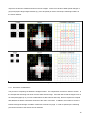
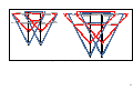
A simple example is presented in Figure 2.4. The target is a simple cross and the search is a larger
(simulated) image. In the upper figure the target is a 5x5 sample and in the lower it is a smaller 3x3 sample.
Correlation coefficients are computed starting with the target placed at the top-left of the search (outer yellow
outline). The correlation coefficient is allocated to the position of the centre pixel of the target (inner yellow
outline). The target is then moved one column to the right and the computation repeated (green outlines)
until the end of the row is reached by the right edge of the target (blue outlines). The target is moved down
one row and the process is repeated generating the correlation coefficients for all possible positions. In this
simple case, the highest correlation coefficient (0.74) is found at the position where the centre of the target is
aligned with the centre of the search - the two white crosses coincide.
The lower part of the figure produces, in general, higher (positive and negative) correlations because of the
similarities of smaller areas (less variation in pixel values). Notice the higher correlation coefficient (0.85) for
the centre location. Also notice that the correlation coefficient for the second position (0.60) is nearly as high
as that for the correct position (0.74) for the larger target and illustrates the possibility of finding incorrect
matches as the target area becomes smaller. Thus, the size of the target window must be considered with
14
respect to the amount of detail and noise in the two images. Areas of low levels of detail (small changes in
grey level) require larger target windows (e.g. 30 to 50 pixels) in order to find unique matching locations in
the search window.
Figure 2.4. An area based image matching example
2.3.1. Geometric considerations
The process of computing correlations is straight forward. The complication comes from where to search. In
the example the searching was done over the entire search image. If the task was to find the target cross on
an aerial photograph (a 14 µm scan creates about 15,000 columns and rows), the time required to compute
225,000,000 correlation coefficients would be of the order of seconds. In addition, the number of incorrect
locations that generate high correlation coefficients could be very high. In order to speed up the matching
process the location of the search area is restricted.
15
The first principle used is to restrict searching along epipolar lines (see Figure 2.2). Epipolar lines are
defined by the coplanarity condition, so once a pair of images has been relatively oriented the relative
locations of conjugate points are known. If a target area is extracted from the left image, the location of the
search array is somewhere along the epipolar line on the right image. If the images were acquired by a strict
translation of the camera in the x image space direction epipolar lines will coincide with rows of pixels. This
is rarely the case.
If the relative motion of the camera includes y and z translations and any or all of the three possible rotations,
the epipolar lines will cut across rows of pixels. When given the location of a target array it is possible to
compute the location of the epipolar line on the search image, searching along and across columns and rows
is not a trivial matter. The problem of cross-row epipolar lines is solved by creating epipolar-resampled
images. Given the location of a target its conjugate will lie along the same row of the search image. In
addition, epipolar-resampled images allow comfortable stereoscopic viewing of the stereopair.
X 1,Y 1,Z1
X 1,Y 1,Z2
y1
Epipolar line
x1
bz
y2
Camera base
(Epipolar axis)
z1
x2
z2
Figure 2.5. x-parallax
Where along an epipolar line will a conjugate point lie? This depends on the distance between the epipolar
axis (camera base) and the model point. For points that have the same XY and different Z model coordinates
the conjugate points will lie along the same epipolar line. See Figure 2.5. For a stereopair oriented so the
16
camera’s z axis is vertical, such points would have the same horizontal coordinates and different heights.
The difference in position on images due to a change in model distance is known as x-parallax.
Instead of searching across a whole row in order to find conjugate points if an estimate of the change in
model distance can be made, the search range is then limited to the possible range of x-parallax in that area
of the model. For objects that exhibit large changes in model distance a larger search range (along the
epipolar line) is required. In order to exploit this geometric aspect fully photogrammetric systems such as
LPS make use of strategies - sets of image matching parameters that describe the target area, search
range and the type of terrain - so that the time consumed doing ATE is kept to a minimum.
One more aspect to image matching that should be understood is that ATE is often done in object space.
The movement of target and search areas is controlled by the definition of the terrain model required.
Terrain models are typically defined by a horizontally defined grid - location, orientation and grid spacing.
The ATE process moves from grid point to grid point and performs image matching to determine the height
of the terrain. For vertically images (camera’s z axis coincides with the vertical) the image plane is parallel to
the horizontal object coordinates so moving the target and search areas across the images corresponds to
changing X and Y. Changing the x-parallax corresponds to changing Z. The image matching process for
photogrammetric software optimised for aerial imagery makes use of this concept.
Using oblique and/or convergent imagery in such systems causes significant problems to such optimised
ATE because he images’ z axis no longer coincides with the object’s Z coordinate system. In the extreme
case of horizontally oriented camera axes, the y image axis corresponds to the Z object coordinate axis and
makes the task of converting x-parallax into Z coordinates impossible. The simple solution to this problem is
to perform ATE in model space after RO and then transform the terrain model with a 3DCT into object space.
2.4. Summary
This chapter has presented the essential photogrammetric theories encompassed in this project. The
information presented is by no means an exhaustive coverage of those theories and the reader is directed to
photogrammetric texts such as Mikhail et al. (2002) and Wolf and Dewitt (2000), and to the LPS User Manual
for detailed discussion.
17
3. Methodology overview
This section describes firstly the philosophy of the methodology, details the 3-dimensional conformal
transformation program developed for this project, and finishes with a brief introduction to preparing LPS for
performing RO block adjustment.
3.1. Methodology
As is explained in the proposal, DPWs such as LPS which are designed for production aerial
photogrammetry have difficulty dealing with oblique and convergent imagery when it comes to the solution of
the EO of the imagery and the ATE. The prime reasons for these difficulties lie in the generation of initial
estimates for the EO parameters and the misalignment of the camera axes and the Z object space
coordinate axis for the ATE. Even when a reliable orientation of oblique imagery is achieved experience with
LPS shows that once the camera axis forms an angle with the Z coordinate axis greater than about 30
degrees the results of ATE become unreliable.
The RO of imagery employs a model space coordinate system where the z axis is normal to the image plane
of the camera, a characteristic similar to that of conventional aerial imagery. The x direction is towards the
exposure station of the second image. In this configuration, the orientation angles of all images in a block
become similar to the relative orientation angles of the images expressed in the object space coordinate
system. The main concern is that of the scale of the model coordinate system. The difference between it
and that of the object space coordinate system can be minimised if the camera base of the first pair of
images is as close as possible to that of the actual camera base. With respect to ATE, the advantage of a
relatively oriented model is that the parallax measurements generated by the image matching process are
translated into z coordinates that are nominally perpendicular to the images, not into Z coordinates
substantially oblique to the image planes. Once the terrain is extracted from a relatively oriented model it
can be transformed into object space by a 3-dimensional conformal transformation.
After development and testing of the proposed method, a revised methodology (Figure 3.1) was adopted.
An additional 2 steps are applied between the initial EO (aerotriangulation, AT) and the ATE step. As the
scale is only approximate when performing the initial AT, the results of the AT are processed with the 3dimensional conformal transformation and the scale factor is applied to the camera base. The AT can then
18
be re-run to produce EO data that should be at the correct scale. The subsequent ATE data should also be
true to scale.
Interior orientation
Relative orientation
Aerotriangulation
3D transformation
Control points
Aerotriangulation
ATE
3D transformation
Control points
Real DEM
Accuracy
assessment
Figure 3.1. Revised methodology
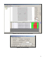
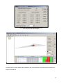
3.2. The 3DCT program
The 3DCT program is written in the C# language using Microsoft Visual Studio 2010. The source code can
be found on the attached DVD. The computation approach is that of a standard non-linear least squares
adjustment and is illustrated in Figure 3.2. The user interacts through the graphical user interface shown in
Figure 3.3.
Three input files are required. The files should be ASCII text files with the structure of Name X Y Z.
Sample data files can be found in Appendix D and on the attached DVD. The three files are:
1. The arbitrary (model space) coordinates of the control points
2. The object space coordinates of the control points
3. The model space coordinates of the DEM to be transformed
19
Input both sets of control point coordinates
Calculate initial approximations for
transformation parameters
Calculate corrections
Add corrections to initial approximations
NO
Correction<0.001
YES
Apply transformation parameters to DEM
Figure 3.2. 3DCT computation flowchart
1
3
2
4
Figure 3.3. 3DCT user interface
The user is required to:
1. Specify the model space control point coordinates (Window 1)
• Click the Import button and choose the text file that contains the model space coordinates of
the control points.
20
2. Specify the object space control point coordinates (Window 2)
• Click Import button and choose the text file that contains the object space coordinates of the
control points.
3. Specify the DEM to be transformed (Window 3)
• This is an optional step and may be skipped if just the transformation parameters are required
either to check the control or to compute the scale factor.
• Click Import button and choose the text file that contains the model space coordinates of the
DEM. The data will appear in the window after a few seconds.
4. Click Calculate to start the transformation. The program has not been optimised for processing
performance and this process may take several minutes depending on the speed of the computer
and the size of the DEM to be transformed. The transformation results will appear in Window 4.
5. Check the transformation results and save the transformed points (Window 4).
• Click the Save transformation results button and specify the file name and location of the
output file. The output file contains the results of the least squares computation at each
iteration, the residuals of the control points, the standard error of unit weight, and the
transformed points. A sample output is shown in Figure 3.4.
• Click the Output points button to save the transformed coordinates to a file.
3.3. Using LPS for a RO block
The normal mode of operation of LPS is to incorporate the object space coordinates of control points in the
AT computation by bundle adjustment. Forcing LPS to use a RO block is quite simple, the steps are
illustrated here using LPS 2011.
3.3.1. Preparation
• Set up a standard LPS project but specify LSR (Unknown) Projection during the block setup. The
result should be similar to that shown in Figure 3.5.
21
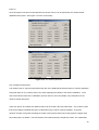
Initial approximations:
Scale = 0.9851
Omega = 0.2026
Phi
= 0.1743
Kappa = -0.0820
TX = -1.9835
TY = 47.6980
TZ = 70.2401
Initial approximations: the initial estimates
of the seven transformation parameters.
Iteration: 1
Param
Scale
Omega
Phi
Kappa
Tx
Ty
Tz
Iteration: iteration step
Correction
0.000
-0.042
-0.012
0.037
2.636
-3.393
2.868
Residuals:
Point X res
B1
-0.0916
B2
0.0829
B3
-0.0393
B4
0.0204
X1
-0.0054
X2
0.0329
New Value:
0.985
0.1605
0.1623
-0.0448
0.6529
44.3052
73.1079
Y res
0.0112
-0.0440
-0.0196
-0.0098
-0.0100
0.0722
Z res
0.002
-0.060
0.032
-0.001
0.008
0.019
Residuals: reflects the accuracy of
control points; the points with large
errors can be deleted for better
standard error of unit weight.
Standard Error of Unit Weight: 0.0533
Iteration: 2
Param
Correction
New Value:
:
:
Residuals:
Point X res
Y res
Z res
B1
-0.0777
0.0170
0.008
B2
0.0635 -0.0054 -0.025
B3
-0.0470 -0.0320
0.015
B4
-0.0069
0.0138
0.012
X1
-0.0007 -0.0313 -0.015
X2
0.0688
0.0378
0.005
Standard Error of Unit Weight: 0.0450
Final Results:
Param
Value
Scale
0.9847
Omega
0.1606
Phi
0.1623
Kappa -0.0448
Tx
0.654
Ty
44.313
Tz
73.106
Stan.Dev
0.0003
0.0692
0.0171
0.0261
1.7668
5.9810
2.6801
Standard Error of Unit Weight:
reflects the general quality of
transformation.
The estimated transformation
parameters.
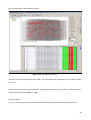
Figure 3.4. 3DCT sample output
22
Figure 3.5. Set coordinate system
Figure 3.6. Frame settings
• Check the Rotation System is “Omega, Phi, Kappa”, the Photo Direction is “Z-axis for normal images”,
and set the approximate flying height to the longest object distance in the project. See Figure 3.6.
• Complete the project set up as normal by adding the photos and doing the IO (if necessary).
• Open the Frame Editor and select the Exterior Information tab. For the first photo set a desired set of
coordinates for X0, Y0, and Z0. Values of zero for X0 and Y0 are generally acceptable but make Z0
larger than the value set for the Average Flying Height. This should ensure the DEM does not have
23
negative heights; something that has sometimes caused difficulties during the ATE. Set the Rotation
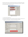
Angles to zero. Set all Status fields to “Fixed”. See Figure 3.7.
Figure 3.7. EO settings for the first image
• Click the Next button and set the X0 value for the second image to the estimated camera base. The
closer this is to the actual camera base the closer the scale of the Model space coordinates will be to
the Object space coordinates. Set the Status of X0 to “Fixed”. All other parameters should be the
same as for the first image but the Status should be set to “Initial”. See Figure 3.8.
Figure 3.8. EO settings for the second image
3.3.2. Processing
• Digitise tie points and any control points visible in the images, perform the AT and check the result.
• When an acceptable solution has been achieved, extract the control point data from the point
measurement interface.
24
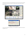
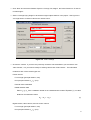
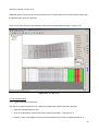
Figure 3.9. Sorting the point data
Figure 3.10. Selected control points
• Firstly, sort the object points by clicking the “Description” column. See Figure 3.9.
• Hold down the left mouse button and drag-select downwards the named control points.
• Control-click the columns for Description, X Reference, Y Reference, and Z Reference. The interface
should look like that shown in Figure 3.10.
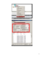
• Initiate the Export dialogue by right-clicking the header row. Set the separator character as “Space” in
25
the export options (see Figure 3.11). Save the data file *.dat (ASCII text) to the desired location.
Remember where you put it.
Figure 3.11. Export options
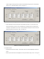
The exported file should contain information of the form:
X2
X1
B4
B3
B2
B1
991.376 1981.932 4717.275
1032.975 2008.809 4711.485
1141.742 2009.419 4676.642
1061.623 2015.501 4701.466
1162.121 1988.438 4668.770
1060.815 1979.879 4709.604
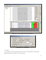
• Invoke the 3DCT program and perform steps 1 and 2 of section 3.2.
• Press the “Calculate” button and save the transformation output.
• Extract the scale parameter from the transformation output and apply it to the camera base, the X0
value shown in Figure 3.8.
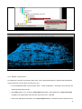
• Re-process the AT and extract the DEM as necessary.
• Using the new AT control point data, transform the DEM.
26
4. Sample projects
Four different projects are presented here. They are a metric film-based project from a helicopter platform, a
non-metric digital-based project from a helicopter platform, a metric film-based terrestrial project, and a handheld, non-metric digital-based terrestrial project. The last project is an example of a project that failed EO
due to poor image scale and object geometry. This project highlights the need for good planning and image
acquisition, not only for unconventional photogrammetric projects, but for all photogrammetric projects.
For the remainder of this section it is assumed the operator is familiar with the basic operation of LPS for
conventional projects as well as for an unconventional (RO) project.
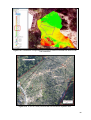
4.1. Tuen Mun Highway slope DEM - helicopter metric film
The objective of this 1996 project was to create a DEM of the existing slope prior to road widening operations.
The imagery was obtained from a helicopter flying as far as possible parallel to the slope at a distance of
about 200 m. The camera used was a Rolleiflex 6006 metric medium format camera. In order to meet the
project specifications the initial project design specified a wide angle (50 mm) lens and an object distance of
50 m which meant a flight path over the roadway. This design was rejected by the Civil Aviation Department
resulting in the fall-back design with a 180 mm lens. This design resulted in much smaller intersection
angles and reduced DEM accuracy.
4.1.1. Project data
Camera calibration data
Principal distance (mm)
:
Principal point offset (x,y,mm) :
Reseau mark coordinates (x,y,mm) :
2
3
4
Radial distortion
:
180.000
0.000
0.000
1
-24.9995 25.0004
25.0004 24.9995
-24.9997 -24.9998
24.9993 -25.0000
Unknown
Control point coordinates (HK80)
Control Point
X1
X2
B1
B2
B3
B4
B5
X (m)
820072.474
820034.477
820082.266
820178.656
820094.921
820166.353
820303.627
Y (m)
824359.451
824381.441
824327.482
824267.423
824346.645
824287.638
824218.859
Z (m)
41.156
14.318
16.643
17.925
46.139
38.569
16.233
27
Imagery
Over 200 photos were obtained for the project, one strip of 12 photos is used in this sample project. The
strip, along with the control point locations is shown in Figure 4.1.
Figure 4.1. The Tuen Mun Highway imagery
4.1.2. Project workflow
Select geometric model
• Select frame camera
Define block properties
• Set SR (Unknown) Projection
• Input 200m for the average flying height (the nominal distance from the slope)
• Input the camera calibration information (save the camera file if required)
Add images to the block
• Select the images and compute image pyramids if necessary
28
Perform IO
• Check that all images are activated
• The four corner reseau marks are used in this project.
• Select the Interior Orientation tab on the Frame Camera Editor
• As the images have been manually scanned and reseau marks are being used instead of conventional
fiducial marks it is necessary to manually digitise them on all images.
• As reseau marks are used you may need to use the image enhancement tools to make the marks
more visible. Increase the brightness and/or decrease the contrast slightly (+/- 10) is usually sufficient.
Initialise EO
• Open the Exterior Orientation tab and fix the left image’s EO. A flying height of 300 m was chosen to
ensure the DEM contained positive heights. The camera base to the second image was estimated as
40 m. The EO data for the first two images are shown in Figures 4.2 and 4.3.
• Click OK and close the Frame Editor.
Figure 4.2. EO for image 1
Figure 4.3. EO for image 2
29
Digitise tie points
• Deactivate all but the first two images. This will allow a quick AT check after digitising the first pair of
photos.
• Start the point measurement tool and digitise the two control points X1 and X2 visible in image 1 and 2.
In this type of orientation these points are Usage = Tie. Control point X2 is shown in Figure 4.4.
Figure 4.4. Control point X2
• Add 4 other tie points evenly distributed in the overlap area of the two photos. See Figure 4.5.
• Save the project and run the AT for the first pair. You should achieve a converged solution. If not,
check the previous steps for blunders. The Project manager should look like Figure 4.6.
• Activate the next image (image 3)
• Open the Frame Editor, set X0 to 80 and copy the remaining EO parameters from image 2.
• Set the Status to “Initial”.
• Digitise control and tie points and execute AT. The first three tie points on image 3 should be the
second three points on image 2.
30
Figure 4.5. Tie points of the first pair
• Repeat the previous 4 steps until the strip is finished.
Auto Tie Points
The reliability of the AT can be improved by adding additional tie points using the Auto Tie Points (ATP)
function. ATP needs to be used with care as having too many points can produce very unreliable results due
to poor matching. Much time can be spent removing those poorly or wrongly matched points.
The suggested mode to use is shown in Figure 4.7. Specifying the strategy or distribution parameters varies
from project to project. For this sample project the default settings were used.
Exterior Initialisation
Computing the initial EO parameters may also be done via the Frame Editor and the Exterior Initialisation
tool. An example of setting for this project is shown in Figure 4.8.
31
Figure 4.6. Project manager after the AT of the first model
Figure 4.7. Auto Tie Point settings
32
Figure 4.8. Exterior Initialisation settings
Using this method worked well for the first 5 images, but as the project is on a curved road segment the
changes in camera base and orientation angles created difficulties with the AT as more images were added
to the block.
If this method is used you still need to fix the EO parameters of the first image and the X0 paramter of the
second image.
33
Initial AT
Once all images have been incorporated into the block a final AT can be performed, the results verified,
updated and accepted. See Figure 4.9 for the AT summary.
Figure 4.9. AT summary
Figure 4.10. AT summary with APs
Use of additional parameters
The results of the AT may be enhanced through the use of additonal parameters (APs) for camera calibration.
Using this option is very useful if there is any doubt regarding the validity of the camera calibration. In the
case of the camera used here a calibration report for the lens was not available, only information for the
camera’s reseau was given.
There are various AP models, the details of which can be found in the LPS Field Guide. The number of APs
that can be reliably estimated during the AT depends on the number of points available. As just the
minimum number of tie points (including the visible control points) were used in this project the higher order
AP models were not reliable. The best solution was achieved with the simples AP model - the 2 parameter
34
radial distortion model. The resulting AT Summary is shown in Figure 4.10.
Additional quality control may be achieved through the AT Properties Blunder Checking options and through
the Review option of the AT Summary.
At the end of processing the Project Manager should look something like that shown in Figure 4.11.
Figure 4.11. The RO block
Export model space coordinates
This step is to create the data file to be used as the model space input for the 3DCT program.
• Open the Point Measurement tool
• Click on the Description column and sort the points as necessary. See Figure 4.12.
• Select the rows of the digitised control points and Shift-Click the columns headed Description, X
Reference, Y Reference and Z Reference. The selection should look like Figure 4.13.
• Right click in the header row and select the Export option. Set the separator character as “Space” in
35
the export options (see Figure 4.14). Save the data file *.dat (ASCII text) to the desired location.
Remember where you put it.
Figure 4.12. Sorting the point data
Figure 4.13. Selected control points
• The exported file should be:
X2
X1
B4
B3
B2
B1
991.376 1981.932 4717.275
1032.975 2008.809 4711.485
1141.742 2009.419 4676.642
1061.623 2015.501 4701.466
1162.121 1988.438 4668.770
1060.815 1979.879 4709.604
36
Figure 4.14. Export options
4.1.3. Updating the scale of the model space coordinates
If you are unsure about the scale of the model space coordinates you can run the 3DCT programme with just
the model and object coordinates of the control points. Check the scale factor of the transformation, update
the camera base and re-run the AT. This process could be repeated until the scale factor is very close to 1.
The scale of the created model for this project was 1.0351 and was considered to be accurate enough for
this Sample project.
4.1.4. DEM extraction.
There are various types of terrain models that LPS can create. This is not a tutorial on the various options
but, rather, it shows how to manage the data created. It is necessary to transform the DEM’s coordinates,
and that the ASCII output type is preferred. However there are LPS/ERDAS tools for converting data in
other formats to ASCII.
Define the file type and form
• Choose ASCII and single mosaic. See Figure 4.15. The single mosaic option will create one file that
contains the whole terrain model. It is created by interpolation from the individual terrain models from
each stereopair.
• Choose an appropriate cell size. This is a critical element when it comes to the final terrain model
resolution. If the initial camera base has been significantly under or over estimated the DEM
resolution will be significantly changed scale following the 3DCT. If the camera base is under37
estimated by 10% the cell size will be enlarged by 10% after the 3DCT.
• Choose all the remaining parameters and execute the ATE.
• Using the default set of parameters and a 0.10 m cell size a DEM of 481,500 points was created.
• It would have been wise to have defined a boundary around just the slope. Extracting the whole
terrain model will show some of the data extraction issues to be considered for other projects. These
will be illustrated later in the report.
Figure 4.15. Necessary terrain model parameters
4.1.5. Coordinate transformation
Three input files are required:
• Model space coordinates of the CPs
• Object space coordinates f the CPs
• Model space coordinates of the DEM points.
Load the three files and press Calculate. When the calculation is done, save the transformed coordinates.
4.1.6. Data output
The terrain model can be viewed in the LPS Terrain Editor and other software after conversion. Two such
38
conversions are shown here. The first one is Leica’s Cyclone point cloud software (.imp) and the second is
ERDAS .img format.
Cyclone point cloud (.imp)
• Give the ASCII DEM output file a .txt file extension.
• Start Cyclone and add a new database (Figure 4.16).
Figure 4.16. Create a new data in Cyclone
• Right click the database file and select Import (Figure 4.17)
• Select DEM text file and set the import parameters as shown in Figure 4.18.
• Click “Import” and accept the default intensity value.
• When the import is completed go to the Navigator and Create and Open a new ModelSpace view as is
shown in Figure 4.19.
• When the ModelSpace view opens you should see the terrain model similar to that of Figure 4.20.
• Upon examining the point cloud, a lot of noise can be found, especially at the edges. Below the base
of the slope and around the vegetated areas exhibit the results of poor image matching. This is
related to the image acquisition, not the processing methodology.
39
Figure 4.17. Importing an ASCII file into Cyclone
Figure 4.18. DEM ASCII file import parameters
40
Figure 4.19.Create and open a new ModelSpace
Figure 4.20. The Tuen Mun Highway DEM
ERDAS .img file format
For analysis in a GIS the .img format is often used. As the transformed data is in ASCII format the ERDAS
Terrain Prep Tool can be used to convert it into .img.
• From the ERDAS toolbar choose Terrain menu > Terrain Preparation > Surfacing Tool to open the 3D
Surfacing dialog (Figure 4.21).
• Click Read (Figure 4.22), check the Points Data radio button; select ASCII File in Source File Type;
navigate to the target folder and select the source file name. Click OK.
• Specify the appropriate information in the Import Options dialog. Remember that the output file from
the 3DCT contains the transformation computation iteration information. Unless you edit the file to
41
remove this information you’ll need to specify the appropriate number of rows to skip. Define the field
numbers to write to the output file. Figure 4.23 shows both tabs of the Import Options dialogue.
• Click OK to import the data. The Surfacing dialogue (Figure 4.24) will now display your terrain model’s
data. Set appropriate DEM parameters. Click OK to create the .img DEM.
Figure 4.21. The location of the Surfacing Tool in ERDAS Imagine
Figure 4.22. 3D Surfacing dialogue
42
Figure 4.23. Import Options
Figure 4.24. Surfacing dialogue
43
4.2. Shatin Pass slope DEM - helicopter non-metric digital
This is a helicopter-based project supplied by CEDD with images taken by a hand-held NIKON D200 camera
with a 105 mm lens. There are 20 images in total, with camera bases of about 10 m. The average object
distance was about 150 m. Note that the camera was oriented with the short side of the frame along the
strip resulting in very short camera bases and lower parallaxes for a given percentage of endlap compared to
if the camera was oriented with the long side of the frame along the strip. There are 12 control points
distributed evenly throughout the block.
The main difference between this and the previous sample project is the geometric model with respect to the
camera. Only those procedures that are significantly different are described here.
4.2.1. Project data
Camera data
Sensor size (mm)
Image size (pixels)
Principal distance (nominal, mm)
Principal point offset (assumed, x,y,mm)
Radial distortion
:
:
:
:
:
23.6 x 15.8
3872 x 2592
105
0.000
0.000
Unknown
Control point coordinates (HK80)
Control Point
M1
M2
M3
M5
M6
M8
M10
RK2
RK3
RK4
RK5
RK6
N (m)
823978.95
823979.84
823972.53
823989.84
823996.90
823984.67
824025.17
824008.25
824003.19
824002.43
823993.30
824009.15
E (m)
839176.65
839193.03
839160.48
839163.04
839168.67
839219.81
839155.51
839176.46
839188.94
839182.55
839193.85
839191.02
RL (m)
370.63
372.31
360.02
371.30
376.47
376.60
403.01
388.68
388.42
384.37
384.38
396.95
An overview of the control point locations is given in Figure 4.25.
Imagery
The 20 images can be seen in Figure 4.26.
44
Figure 4.25. Control point locations
4.2.2. Project workflow
Model Setup
Select Digital Camera as the geometric model. See Figure 4.27.
Figure 4.27. Model Setup
Perform IO
The IO for a digital camera is very simple once the pixel size is computed. This should be done for both the
x and y sensor dimensions. Pixels should be square. One difficulty in this computation is the relationship
between the physical sensor size and the area occupied by the active area of the sensor. Finding this
45
Figure 4.26. Images of the Shatin Pass project
relationship without a rigorous calibration is difficult. In the case at hand the approximate pixel sizes are
computed according to Equations 4.1.
Pixel size in x =
CCD size in x
23.6mm
=
= 6.1μm
number of pixels in x
3872
CCD size in x
15.8mm
Pixel size in y =
=
= 6.1μm
number of pixels in x
2592
(4.1)
46
Enter these values in Digital Camera Frame editor and check Apply to all of active frames as shown in
Figure 4.28.
Figure 4.28. Interior orientation
Perform EO
All the steps in this process are the same as for the Tuen Mun sample project. The final results of the AT are
shown in Figure 4.29.
Figure 4.29. Triangulation Summary
It is worthwhile to note that the triangulation result is much better than the Tuen Mun project. The prime
reason for this is the image scale. An overview of the block can be seen in Figure 4.30.
Check 3DCT and re-triangulation
The results of the first transformation showed residuals for control points M3 and M8 of over 1 m. These
47
were removed and the transformation redone.
Figure 4.30. The Shatin Pass block
The scale of the second processing was 0.6835. The camera base was changed from 10 m to 6.8 m and the
AT re-run.
The processing of the second AT results (also with M3 and M8 removed) gave a scale of 1.005 and showed
a slight improvement in the RMSE to 0.2269.
Terrain extraction
A 1 m by 1 m terrain model was extracted from the whole area and imported into Cyclone (Figure 4.31).
48
Figure 4.31. The Shatin Pass DEM in Cyclone
4.3. Ap Lei Chau landslide - terrestrial metric film
This is a very old CEDD project taken with a tripod mounted Hasselblad MK70 camera with a 60 mm lens.
Only the calibrated principal distance was available and a statement that lens distortion is “less than 10 µm”.
A set of 29 convergent photos were taken from 5 locations. There are 7 control points.
4.3.1. Project data
Camera calibration data
Principal distance (mm)
Principal point offset (x,y,mm)
Reseau mark coordinates (x,y,mm)
Radial distortion
:
:
:
:
61.06
0.000
Unknown
Unknown
0.000
Control point coordinates (HK80)
Control Point
M1
M2
M3
M4
M5
M6
M7
X (m)
833749.72
833749.04
833756.19
833746.26
833723.20
833719.91
833732.04
Y (m)
811584.77
811583.96
811575.00
811552.46
811572.14
811583.31
811590.04
Z (m)
30.14
35.30
38.01
60.84
46.18
36.42
29.43
Imagery
Because of the complex nature of the imagery, a sample of 3 photos (numbers 1, 2 and 7) is used in this
project. The strip, along with the control point locations, is shown in Figure 4.32.
49
M4
M5
M3
M2
M6
M1
M7
Figure 4.32. Ap Lei Chau imagery and control
4.3.2. Processing issues
There were several problems to be solved in this project:
• The coordinates of the reseau marks. No calibration was available.
• The image quality. Very poorly exposed.
• The initial EO values. The layout diagram did not seem to agree with the markings on the proof sheet.
Reseau coordinates
No information relating to the nominal coordinates of a MK70 reseau could be found. The solution was to
measure the bounding rectangle of the four corner grid points. The measurements showed a 40.11 mm
square. The coordinates of all 25 reseau marks were computed by even division of that dimension (Table
4.1). All reseau marks were used in the IO.
Table 4.1. CEDD MK70 Reseau coordinates
x
y
x
y
x
y
x
y
x
y
-20.055
20.055
-20.055
10.0275
-20.055
0
-20.055
-10.0275
-20.055
-20.055
-10.0275
0
10.0275
20.055
20.055
20.055
20.055
20.055
-10.0275
0
10.0275
20.055
10.0275
10.0275
10.0275
10.0275
-10.0275
0
10.0275
20.055
0
0
0
0
-10.0275
0
10.0275
20.055
-10.0275 -10.0275 -10.0275 -10.0275
-10.0275
0
10.0275
20.055
-20.055
-20.055
-20.055
-20.055
Image quality
A set of diapositive images had been scanned in 1995 by Leica. The diapositives were only in fair condition
with several scratches visible. Before being used the images were enhanced using the auto-levels function
of Photoshop v5.
50
Initial EO estimates
The imagery had been taken in a combination of parallel and convergent axis orientations. Establishing the
exact relationship between the numbered images and their exposure stations was difficult because it was
found the photo numbering with respect to the exposure station locations did not agree with the information
recorded on the station diagram. An approximate camera base of 5 m was scaled from the station diagram
but the orientation angles had to be estimated by the AT. Careful assessment the results of each AT
iteration was required.
4.3.3. Processing results
Due to the convergent nature of the block the whole AT process was done manually. No attempt to use the
ATP function was made. The AT made use of the 7 control points and 3 additional tie points. Due to the
nature of the terrain finding clear and easily identifiable tie points was a difficult task, especially at the back of
the scene.
The initial AT result is given in Figure 4.33.
Figure 4.33. Triangulation Summary for initial block processing
The high RMSE was attributed to the lack of calibration information. Each of the AP models was applied.
The best result was produced by the 12 parameter Ebner model (see Figure 4.34). The AT report is
summarised in Figure 4.35 and Project Manager is shown in Figure 4.36.
51
Figure 4.34. Triangulation Summary with the Ebner APs
The exterior orientation parameters
image ID
Xs
Ys
1
0.0000
0.0000
2
4.0000
-0.5458
3
2.5890
-0.2842
The coordinates of object points
Point ID
X
Y
1
-0.7062
-1.1357
2
-0.5515
-0.3524
3
-1.1825
-0.2538
4
-0.6178
0.8898
5
0.9815
0.1832
6
1.6844
-0.4722
7
1.1674
-1.0861
8
0.3332
-0.5357
9
1.2669
-0.7284
10
-1.3075
0.0972
11
-0.8125
0.1088
The total object points = 11
Zs
20.0000
18.0965
19.1860
OMEGA
0.0000
8.2786
4.5023
Z
15.8428
15.3044
15.0050
13.5862
13.8208
14.3135
15.2998
15.2944
15.0821
14.9035
14.5334
PHI
0.0000
42.0536
27.6467
KAPPA
0.0000
-18.2938
-15.0017
Overlap
3
3
3
3
3
2
3
3
3
3
3
Total mean error of 32 image points: ax=0.013, ay=-0.000
Total RMSE of 32 image points: mx=2.344, my=3.976
Figure 4.35. Abstract of AT report
While the result is a significant improvement, an RMSE value of 9 (pixels) is still large. The AT report shows
RMS values of 2.3 pix and 4.0 pix for the x and y image coordinates respectively. Careful inspection of the
digitised points did not reveal any point identification problems. The cause of the large residuals must be
due to incorrect assumptions regarding the camera.
The orientation angles, especially φ, are quite large. The value for image 2 is 42°, more appropriate for a
close-range discrete point measurement project than one designed for terrain extraction.
52
Figure 4.36. Project Manager showing the ground coverage of the block
The initial 3DCT results were very poor showing a scale of 13.5 and RMS residuals on the control points of
2.8 m, 3.1 m, and 2.7 m for X, Y and Z respectively. No further processing was attempted.
4.3.4. Conclusion
Convergent imagery combined with uncertainties regarding the camera parameters make for an unreliable
project. Where terrain extraction is the prime objective, parallel or low-convergence imagery is necessary.
4.4. Tai O breakwater DEM - terrestrial non-metric digital
This project did not get very far into the processing chain. A single strip of 7 images was acquired with a
Nikon D3s with a 70-200 mm zoom lens set at 70 mm. A set of calibration parameters from PhotoModeler
was supplied as was a set of control point coordinates.
4.4.1. Imagery
Figure 4.37 shows 6 of the 7 photos and the control point locations.
53
4066
4069
4073
4077
4081
4085
Figure 4.37. Six out of seven of the Tai O breakwater images showing control
It is clear this is a very poor photogrammetric block for several reasons:
• Scale. The object only occupies about 5% of the frame. The possibility of computing an orientation
based on measurements on the object will be very low.
• The endlap is insufficient, particularly between the first three images. LPS requires at least 50%
endlap for a solution.
4.4.2. Camera calibration
The imagery was accompanied by a screen capture of a PhotoModeler calibration (Figure 4.38). The sensor
sizes correspond to the nominal dimensions of a Nikon D3s digital camera. This is a professional "full frame"
camera that has nominal sensor dimensions of 36 mm x 24 mm. The calibrated dimensions are very close
to these values. At 79.395, the calibrated principal distance is 9.395 longer than that recorded in the exif
data of the images. It can only be concluded that principal distance was obtained with the camera focused
at approximately 600 mm and not (at least) at the hyperfocal distance as would be required for these images
to be in focus.
54
Figure 4.38. PhotoModeler D3s calibration
The dimensions of the sensor produce a pixel size of 8.46 µm.
Evaluation of the radial distortion parameters yields a maximum value of 15 µm at the very edge of the frame
and 10 µm at a distance of 15 mm from the principal point. The latter value is less than 2 pixels and, as the
calibrated principal distance is not reliable, the radial distortion parameters were also ignored.
The calibration parameters used for the processing of this project are:
Sensor size (mm)
Image size (pixels)
Pixel size (µm)
Principal distance (nominal, mm)
Principal point offset (x,y,mm)
Radial distortion
:
:
:
:
:
:
36.0000 x 23.9549
4256 x 2832
8.46
70
0.000
0.000
0.0
4.4.3. Processing
The same processing methodology as for Sample Project 2 was adopted. The initial AT solution failed but
the RMSE was quite small. Adopting the orientation and re-running the AT produced the solution shown in
55
Figure 4.39.
Figure 4.39. AT solution for images 1 and 2
The Project Manager shows the orientations in Figure 4.40.
Figure 4.40. The orientation of the first two images
Image 3 was added with the result of a significantly larger RMS error (Figure 4.41) and a very distorted set of
orientations (Figure 4.42).
56
Figure 4.41. Triangulation Summary of the initial
processing of the first three images
Figure 4.42. Project manager showing the EO of the first three images
Accepting the AT results, updating the orientations and re-processing the AT produced the result shown in
Figures 4.43 and 4.44.
57
Figure 4.43. Triangulation Summary of the final
processing of the first three images
Figure 4.44. Project Manager showing the updated EO
Adding in the fourth image resulted in complete failure of the AT. No manipulation of the initial orientation
parameters could coax LPS to produce a solution for the AT.
58
4.4.4. Additional processing
In order to determine if the difficulty experienced in obtaining a reliable RO, the imagery was also processed
with the StereoMaker (SMK) module of 3D Mapper's 3D Desktop Photogrammetry System and with
PhotoModeler version 4.0. Both of these photogrammetric systems had difficulty in obtaining RO results,
even with a single pair of images.
4.4.5. Conclusion
The failure of this project was caused by the imaging geometry, with some contribution of the camera
calibration. The image scale was insufficient to enable a reliable EO to be computed as the object occupied
a very narrow portion of the image and the end laps were insufficient to allow LPS to estimate the orientation
angles. It is doubtful that such a photogrammetric strip could be processed by other photogrammetric
systems.
59
5. Independent validation
To ensure that the tool works properly when being operated by the potential users, both the software and the
workflow are tested by the staff of CEDD Survey Division, who did not take part in the development of the
tool. The images of Shatin To Shek Fresh Water Service Reservoir, which were taken in another helicopterbased project, are adopted as the test data and the accuracy of the product is assessed. A sample image is
presented in Figure 5.1 and the locations of control and check points in Figure 5.2.
Figure 5.1. The appearance of the subject hillside of the project
5.1. Project data
5.1.1. Camera data
Camera
:
Sensor size (mm)
:
Image size (pixels) :
Lens
:
Principal point offset
Radial distortion
:
Nikon D3s
36mm x 24mm
4256 x 2832
Nikon AF-Nikkor 50mm f/1.4D
(x,y, mm) : 0 0 (assumed)
unknown
5.1.2. Control point coordinates (HK80)
Control Point
P1
P3
P6
P7
P9
P11
N (m)
826082.821
826073.198
826056.999
826061.946
826025.381
826024.972
E (m)
839021.921
839012.631
839033.936
839099.957
839084.737
839052.648
RL (m)
142.118
135.679
134.848
167.825
155.359
141.239
60
5.1.3. Check point coordinates (HK80)
Check Point
P4
P8
N (m)
826066.829
826067.716
E (m)
839025.058
839056.982
RL (m)
138.556
149.349
Figure 5.2. Location of control points and check points
5.1.4. Imagery
A strip of 8 photos is used in this test and it is shown in Figure 5.3.
Figure 5.3. The imagery of Shatin To Shek Fresh Water Service Reservoir
61
5.2. Testing of the workflow
Figure 5.4 summarizes the workflow of using the methodology. The test goes through the procedure step by
step.
Step 1: Create a new LPS project and define projection as LSR (Unknown)
Step 2: Input flying height (object distance in unconventional project) and camera
information
Step 3: Add images
Step 4: Perform Interior Orientation
Step 5: Input Exterior Orientation information
Step 6: Digitize manual tie points
Step 7: Run auto tie points extraction
Step 8: Perform aerial triangulation (AT) and examine the AT Report to remove those large
residue tie points
Step 9: Enhance AT result by selecting the proper additional parameter (AP) model
Step 10: Export control points in model space
Step 11: Run 3DCT program to check scale factor of transformation
Step 12: Change camera base of second photo by multiplying a scale factor generated from
previous transformation
Step 13: Re-run AT and 3DCT until the scale factor tends to 1
Figure 5.4. The workflow of using the established methodology
Step 1 to Step 4 are standard procedures in an LPS project. But one must be aware of the necessity to
obtain an estimation of the object distance, which may not be easy in helicopter-based project, as input data
in Step 2. In this project, a laser range finder was employed during the flight.
In Step 5, another important piece of information required is the camera base of the first pair of photos.
Although only an approximate value is required, initial planning of how to acquire this information is essential,
particularly on a mobile platform. In this project, a top mount GPS unit was attached to the camera and the
camera base was derived from the coordinates tagged to the photos.
62
Afterwards, eight control points were manually digitised (Figure 5.5) and some other tie points are generated
by automatic tie point extraction with an intention of creating 30 points per image as shown in Figure 5.6
(Step 6 and Step 7).
Figure 5.5. Manual digitising of tie points
Figure 5.6. Automatic tie point extraction
Having the tie points defined, AT follows (Step 8). The AT report (Figure 5.7) revealed that the resulting unitweight RMSE is 0.7341.
63
Figure 5.7. AT report
To enhance the AT result, those tie points with large residuals were removed and additional parameter (AP)
model is adopted (Step 9). Different AP models are available in LPS and Jacobsen’s simple model provided
the best result in this project. The resulting unit-weight RMSE value improved to 0.3840 (Figure 5.8).
Figure 5.8. Lens calibration AP model selection and AT result
The coordinates of the control points in model space are extracted (Step 10) after running AT and are input
to 3DCT program together with the surveyed coordinates for transformation (Step 11). After calculation, the
scale was found to be 1.192 (Figure 5.9).
To improve the model accuracy, the scale obtained was applied to the initial camera base as a factor. The
initial camera base was therefore changed to 8.495 m (7.127 m x 1.192) with other parameters being kept
unchanged (Step 12, Figure 5.10).
AT was performed again with the result slightly improved to 0.3719 (Figure 5.11).
64
Figure 5.9. Result of the first 3D conformal transformation
Figure 5.10. Applying the scale factor to the initial camera base
Figure 5.11. Result of second AT
65
The transformation scale was checked again with the same set of control points by 3DCT program and a
great improvement found. The scale derived was initially 0.9931 and is then improved to 1.000 after 4
iterations (Step 13, Figure 5.12).
Figure 5.12. Result of the final 3D conformal transformation
A 0.2 m grid digital terrain model in ASCII format was generated by the ATE function of LPS (Step 14). The
DTM file was then transformed into the object coordinate system with 3DCT program for further analysis
(Step 15).
5.3. Assessment of Accuracy
To assess the accuracy of DEM points generated from the test site, two comparison methods were applied.
On the one hand, a point comparison method is employed to check the transformed LPS coordinates against
GPS surveyed coordinates of the control points. On the other hand, we carried out surface comparison
method by assessing the difference between the model surface produced by the tool and a surface produced
by an airborne LiDAR point cloud (specifications given in Table 5.1).
5.3.1. Point Comparison
A total of 6 control points and 2 check points (as indicated in sections 5.1.2 and 5.1.3 respectively) were
used for point comparison. The results generated by 3DCT are presented in Table 5.2. In Table 5.2, the
greatest discrepancies in Northing, Easting and Reduced Level of the control points are highlighted in red
while those of the check points are in blue. The RMS error for control points and check points are 0.5m and
66
0.4m respectively.
Table 5.1. Specification of LiDAR survey
0 to ±20°
Field of View
Sidelap
40%
Number of return pulses
up to 4
Average point spacing (m)
0.5
Horizontal accuracy (m, 95% confidence)
0.3
Vertical accuracy (m, 95% confidence)
0.1
Table 5.2. Results of point comparison
Model by 3DCT Transformation
Surveyed Control (by RTK)
Difference
(Model - Surveyed)
N
E
RL
N
E
RL
Diff. N
Diff. E
Diff. H
Remarks
P1
826083.703
839022.385
142.360
826082.821
839021.921
142.118
0.882
0.464
0.242
Control Point
P3
826073.647
839012.752
135.696
826073.198
839012.631
135.679
0.449
0.121
0.017
Control Point
P6
826056.147
839033.844
135.105
826056.999
839033.936
134.848
-0.852
-0.092
0.256
Control Point
P7
826062.541
839099.006
167.680
826061.946
839099.957
167.825
0.595
-0.951
-0.145
Control Point
P9
826025.242
839084.688
155.176
826025.381
839084.737
155.359
-0.139
-0.049
-0.183
Control Point
P11
826024.037
839053.154
141.051
826024.972
839052.648
141.239
-0.935
0.506
-0.188
Control Point
0.702
0.483
0.189
RMS
RMS
P4
826066.955
839025.596
138.426
826066.829
839025.058
138.556
0.126
0.538
-0.130
Check Point
P8
826067.770
839056.466
149.894
826067.716
839056.982
149.349
0.054
-0.516
0.545
Check Point
0.097
0.527
0.396
RMS
RMS
5.3.2. Surface Comparison
In order to have an overview of the accuracy of the site, a 1 m grid surface model of both the 3DCT model
and a LiDAR data point cloud was generated in ArcGIS for surface comparison. The respective height
differences were computed through a simple raster base layer subtraction algorithm. The result of the
subtraction is shown in Figure 5.13.
The comparison reveals that the variance between 3DCT transformed model surface and the LiDAR data
surface is gentle. Most of the height differences fall between -0.5m and 1.5m in the area bounded by the
control points. Some larger discrepancies are located in dense vegetation area (refer to Figure 5.14) which
is outside the control point bounded area and are most likely due to the difference between the image
matched DEM created by photogrammetry and represents the visible surface and the LiDAR DEM that
represents the ground surface due to LiDAR’s ability to penetrate vegetation. Other great discrepancies in
deep red colour are noise which has not been removed in the 3DCT transformed model.
67
Figure 5.13. Visualization of height differences between surfaces extracted from 3DCT model
and LiDAR data
Figure 5.14. A view of control point bounded area and dense vegetation area
68
5.4. Conclusion
The test of the methodology and transformation tool with the use of oblique photos taken from helicopter at
Shatin To Shek Fresh Water Service Reservoir reveals that the stated procedures and the developed
software (3DCT) can be successfully employed in LPS to create a terrain model from unconventional oblique
photos in production environment. However, some points are worth mentioning:
• Camera calibration files from different photogrammetric software cannot be directly input into LPS.
Some additional computations are required.
• On a mobile platform such as helicopter, it is suggested to adopt a shorter camera base with more
overlap so as to effectively counter against the effect of the geometrical variation induced by nonparallel camera axes and non-uniform camera bases of oblique photos.
• Adequate numbers of common control points and manual tie points are important, or automatic tie
point extraction may fail otherwise. It is suggested to have at least 4 common control points and tie
points with even distribution for each pair of images. Besides, during automatic tie point extraction, 15
to 20 ties points should be generated in each image for AT block computation.
• The result of the accuracy assessment is considered satisfactory in this project of which the subject
site was densely vegetated with only limited definite-shaped ground features around for matching as
tie points. The DEM generated can be practicably used for general slope or hillside inspection and
approximate measurement. It is believed that the accuracy of the product can be improved by
enhancing the field procedure. Detailed discussion about this can be found in Chapter 6.
69
6. Field procedures
Based on the outcomes of the test projects presented in this report it is clear that creating DEMs using ATE
in LPS is more successful when the camera axes are near parallel compared to when they are convergent.
The recommended approach for unconventional projects is to use parallel imaging as far as is possible. This
section firstly presents the essential relationships required for the planning of an unconventional project.
Photographic considerations such as shutter speed, sensor sensitivity, and depth of field are not addressed.
Secondly it presents some complicating issues that could be considered during the design of an
unconventional project. And thirdly it outlines a set of procedures that may be adopted when planning field
work for image acquisition in two scenarios:
• Terrestrial image acquisition
• Helicopter image acquisition
In this discussion the term model space rather than object space is used. The purpose of doing this is to
remind the reader that this report deals with unconventional imagery being used in conventional aerial
photogrammetric software. Based on the methodology adopted to process such imagery, measurements are
made in model space and transformed into object space. Model spaces adopts a coordinate system whose
X, Y coordinates are parallel to the image plane of one of the images. The Z coordinate direction is along the
camera axis of that image. Despite this, the term “Object distance” means the distance along the (negative)
Z axis from the camera’s perspective centre to the object. The scale of the model space referred to here is
the same as that of object space.
6.1. Essential relationships
There are several relationships that are required for project planning:
1. Image scale, s, and required object distance, O
2. Ground sample distance, GSD
3. Ground coverage, G
4. Endlap, E%, and camera base, B
5. x-parallax, p
6. Object distance precision, σ
7. Number of images required, N
70
8. Control point distribution
6.1.1. Image scale, s and required object distance, O
The scale of an image is given by Equation 6.1
s=
d
f
=
= 1: S
D O
(6.1)
where d is the distance on the image that corresponds to distance D on the object; f is the nominal focal
length of the lens; and S is the scale number.
This equation serves two purposes:
1. To compute the necessary scale of the imagery based on the required model space (image plane)
coordinate precision defined by the required model-space precision (D) and the per-pixel
measurement precision (d).
2. Compute the required object distance (O ) once the focal length (f) has been determined.
6.1.2. Ground sample distance, GSD
GSD is the distance one image pixel covers in model space and is defined as:
GSD =
i
=i∗S
s
(6.2)
where i is the dimension of a single pixel (pixels are assumed to be square).
GSD applies only to the object distance (O ) where scale is correct. For shorter object distances GSD will be
smaller and will be larger for greater distances.
6.1.3. Ground coverage, G
The area covered by the image at the object distance where the scale is correct. For rectangular images two
values of G should be computed: one for the long side of the image (G ) and one for the short side (G ).
where F is the dimension of side of the image.
G=
F
= F∗S
s
(6.3)
G varies with object distance in the same way as GSD.
71
6.1.4. Endlap, E%, and camera base, B
Endlap is the amount successive images overlap along the direction of the camera base (B). It is typically
expressed as a percentage of the ground coverage (G) of the overlapping dimension of the image. If the
camera is held in the normal position, endlap occurs along the long side of the image, and along the short
side of the image when held in the rotated position. The three components are related to each other by
Equation 6.4:
G'B
Π100%
G
E%
B & G Π+1 '
.
100
E% &
(6.4)
When endlap is defined, the camera base can be computed.
Figure 6.1. x-parallax and parallactic angle
6.1.5. x-parallax, p
x-parallax is the difference in position of conjugate points along the epipolar line on a pair of overlapping
images and is related to B, f and the object distance (O) to the point in model space by Equation 6.5:
p & x u ' x" &
BŒf
O
(6.5)
72
where x’ and x” are the x image coordinates along the epipolar line measured with respect to the principal
points of the images. For a given pair of overlapping images increasing B will increase p . Points closer to
the camera will have greater p than points further away. These relationships are illustrated in Figure 6.1.
Also shown is the concept of parallactic angle (θ). As x-parallax increases so does the parallactic angle.
6.1.6. Object distance precision, σ
The last item is to assess the precision of the object distances. From Equation 5.4 object distance is given
by Equation 6.6:
O=
B∗f
p
(6.6)
From the General Law of Propagation of Variances, the precision of O is given by:
*
0
∂O 0
σ = O_
e ∗ σ0 Q
∂p
(6.7)
where σ0 is the precision of measuring a point on an image. As there are two possible camera bases
involved, there are two possible precisions; one for the long base and the other for the short base.
The important characteristic of Equation 6.7 is that as the object distance gets larger (p gets smaller) the
precision of that distance gets lower (proportional to
*
b
) - points closer to the camera will have higher
precision.
6.1.7. Number of images, N
There are many approaches to this part of project planning. This guide will take a very simple approach -
only one strip of imagery across an area of width W will be acquired. The orientation of the camera (normal
or rotated) may be chosen in order to minimise the number of images but the consequence of using a rotated
camera on the precision of O must be kept in mind.
N = 3+
W
B
(6.7)
Check that the ground coverage is adequate for the vertical side of the image. For example if the camera is
held in the normal orientation that the coverage of the short side is greater than the corresponding dimension
of the project area.
73
6.1.8. Control point distribution
The number and location of control points is highly dependent upon access to the project site. As the control
is used only for transforming the model space coordinates into object space, their number is not as great as
if they were used directly in the AT. The absolute minimum number of control points is 3, but this dos not
provide adequate redundancy for reliable quality control in the 3DCT. It is recommended that at least 6
control points are used with two of them being used as check points. A highly desirable number of control
points is that, for 60% endlap imagery, 4 control points appear towards the corners of the first and last image
pairs and a pair of control points appears in the triple
triple overlap area of every fourth image. This layout is
illustrated in Figure 6.2. Additional points may be established throughout the project area to be used as
check points.
Figure 6.2. Control layout for 10 photos.
6.2. Complicating issues
There are two issues that complicate the design decisions for a project:
1. The choice of lens focal lengths
2. The depth of the project area
These two issues could occupy complete chapters themselves so just the concepts (suitably illustrated) are
presented here.
6.2.1. Choice of focal length
A given image scale may be satisfied by a range of focal length and object distance combinations. For
example, if there are two lenses to choose from; one with f = 20 mm and one with f = 50 mm, a scale of
1:1000 will be achieved with object distances of 20 m and 50 m respectively. Which one should be chosen?
74
Figure 6.3. Parallactic angle and camera base
Firstly, consider site constraints. Does either distance present difficulties in access? If one produces an
object distance that is either too close or too distant there is no choice to be made. Secondly, if both object
distances are possible, choose the shortest focal length lens. In order to optimise the performance of
software such as LPS, imaging matching performs
performs best when the camera axes are parallel. For parallel
imaging geometry shorter focal length lenses produce larger intersection angles and, hence, more precise Z
model coordinates than longer focal length lenses. For a given object distance, as the camera base
increases so does the parallax and parallactic angle. Both these quantities are subject to the influence of the
Base:Object distance ratio (B:O). For two sets of imagery of the same scale but taken with different focal
length lenses, B:O for the longer focal length set will be smaller than for the shorter focal length set. The
parallactic (intersection) angle and x-parallax for the longer focal length imagery (blue lines) will be smaller
than for the shorter focal length imagery (red lines). This is illustrated in Figure 6.3. The basic principal is to
75
use the shortest focal length lens that allows the project to be photographed.
6.2.2. Depth of the project area
Unlike aerial imagery where the range of object depth compared to the object distance is quite small (e.g.
10%), that for a terrestrial- or helicopter-based project may be very large (200% or more). This complicating
factor has a wide range of implications that include variations in:
• Scale
• Coverage
• x-parallax (parallactic angle)
• Z coordinate precision
After the required object distance has been computed, when the project has a considerable (say greater than
50%) amount of depth compared to the object distance a decision needs to be made as to where to define
the object distance from. There are several possibilities:
1. At the furthest part of the project area
2. At the closest part of the project area
3. Somewhere within the project area
4. Divide the project area into depth zones
Figure 6.4 illustrates the impact of the first two choices has on the coverage of a pair of images of different
focal lengths where the project has a depth of 50% of the short focal length lens O . The short focal length
(wider angle, red lines) lens has greater change in coverage as the object distances changes compared to
the longer focal length lens (blue lines). The left side of Figure 6.4 shows that when the furthest point in the
project area is chosen to establish O the wide angle lens will have less coverage at the nearest project point
compared to the longer focal length lens. When the nearest project point is chosen, the right side of the
figure shows the shorter focal length lens will cover more of the object at the furthest project point. As can
be seen, choosing the nearest project point will mean the scale of the image at the furthest will be less than
that required.
When a pair of overlapping images is considered additional factors such as endlap, x-parallax, and σ come
into play. For example, an additional factor related to x-parallax is the search range required during image
76
Figure 6
6.4. Coverage of two focal lengths at two project distances
77
Figure 6.5. The impact of object distance on overlap
78
matching. The impact of variations in endlap are illustrated in Figure 6.5.
In the first case (the left figure), with an endlap of approximately 60% at the furthest part of the project area it
can be seen that the overlap area at the closest part of the area is just less than 50% for the longer focal
length images and significantly less for the shorter focal length images. Obviously this is not a desirable
outcome as a DEM could not be extracted for the whole project area. Increasing the endlap (reducing the
camera base) will reduce the magnitude of the problem at the expense of reducing parallactic angles and
hence ‘’ .
In the second case, full coverage is obtained at the closest part of the project area and the wide angle lens
has increased coverage at the furthest part indicating a larger change in scale compared to the longer focal
length lens. For both lenses the parallactic angles become increasingly narrow towards the furthest part of
the project area. Another undesirable result.
6.3. A terrestrial example
This example is loosely based on the Ap Lei Chau project. A slope is to be photographed and a DEM
created. Specifications are:
• Project area
o Width: 100 m
o Height: 30 m
o Depth (closest to furthest): 20 m
o X, Y precision: 0.01 m
• Camera specification
o Sensor size: 24 mm x 16 mm
o Pixels: 3600 x 2400
o Pixel size:
0“
1”--
&
*”
0“--
& 6.7μm
o Measurement precision: 0.5 pix
o Focal length: 20 mm
• Design endlap: 60%
79
6.3.1. Image scale,s and object distance, O
s=
6.7
d 0.5 ∗ 1000
=
= 1: 3000
D
0.01
f
O = = 0.020 ∗ 3000 = 60 m
s
6.3.2. Ground sample distance, GSD
i
GSD = = i ∗ S = 6.7 ∗ 10^” ∗ 3000 = 0.02 m
s
6.3.3. Coverage, G
G = S ∗ F = 3000 ∗
G = S ∗ F = 3000 ∗
6.3.4. Camera base, B
B = G ∗ _1 −
B = G ∗ _1 −
6.3.5. Parallax at O
p =
p =
6.3.6. Precision of O (Z coordinates)
σ
σ
–
™
24
= 72 m
1000
16
= 48 m
1000
E%
e = 72 ∗ 0.4 = 28.8 m
100
E%
e = 48 ∗ 0.4 = 19.2 m
100
B ∗ f 28.8 ∗ 20
=
= 9.6 mm
O
60
B ∗ f 19.2 ∗ 20
=
= 6.4 mm
O
60
*
*
*
*
0
0
−B ∗ f
28.8 ∗ 20 0
0
= —O
Q
∗
2
∗
σ
˜
=
O_
e ∗ 2 ∗ +0.5 ∗ 6.7.0 Q = 0.016 m
0
0
9.6
p
0
0
0
−B ∗ f
19.2 ∗ 20 0
= —O
Q ∗ 2 ∗ σ0 ˜ = O_
e ∗ 2 ∗ +0.5 ∗ 6.7.0 Q = 0.024 m
0
0
6.4
p
0
80
6.3.7. Number of images, N
N &3+
Width
100
=3+
= 6.5 → 7
B
28.8
Coverage of short side is 48 m, height of area is 30 m and so normal orientation of the camera is appropriate.
6.3.8. Complicating issues
If a 50 mm lens was also available, what would the computations produce?
6.7
d 0.5 ∗ 1000
= 1: 3000
s= =
0.01
D
GSD =
O =
f
= 0.050 ∗ 3000 = 150 m
s
i
= i ∗ S = 6.7 ∗ 10^” ∗ 3000 = 0.02 m
s
G = S ∗ F = 3000 ∗
G = S ∗ F = 3000 ∗
B = G ∗ _1 −
B = G ∗ _1 −
p =
p =
σ
σ
–
™
24
= 72 m
1000
16
= 48 m
1000
E%
e = 72 ∗ 0.4 = 28.8 m
100
E%
e = 48 ∗ 0.4 = 19.2 m
100
B ∗ f 28.8 ∗ 20
=
= 9.6 mm
O
60
B ∗ f 19.2 ∗ 20
=
= 6.4 mm
O
60
*
*
*
*
0
0
−B ∗ f
28.8 ∗ 50 0
0
0
= —O
Q
∗
2
∗
σ
˜
=
O_
e
∗
2
∗
+0.5
∗
6.7.
Q
= 0.040 m
9.60
p0
0
0
0
−B ∗ f
19.2 ∗ 50 0
0
= —O
Q
∗
2
∗
σ
˜
=
O_
e ∗ 2 ∗ +0.5 ∗ 6.7.0 Q = 0.061 m
0
0
6.4
p
0
N =3+
Width
100
=3+
= 6.5 → 7
B
28.8
As expected, most values are unchanged compared to the 20 mm lens, those that are different are
highlighted in yellow. The most significant result is the reduction in σ by a factor of 2.5. Clearly, unless
using the 20 mm lens is not possible, using the 50 mm lens does not provide comparable precision in Z.
81
The effects of choosing the nearest and furthest parts of the project area to set O are summarised in Table
6.1. The key results from this data are:
Table 6.1.
Focal length, mm
setting results
20
50
40
130
X, Y precision, m
2,000
2,600
p , mm
0.007
0.009
14.4
11.1
σ –, m
9.6
7.4
σ ™, m
0.007
0.030
0.011
0.045
48
62.2
32
41.6
40
54
80
170
X, Y precision, m
4,000
3,400
p , mm
0.013
0.011
7.2
8.5
σ –, m
4.8
5.6
σ ™, m
0.029
0.052
0.043
0.078
96
81.6
64
54.4
70
65
at furthest project distance
O to nearest point, m
Scale number, S
p , mm
G ,m
G ,m
E%
at nearest project distance
O to furthest point, m
Scale number, S
p , mm
G ,m
G ,m
E%
1. Despite the greater variation in σ between the two settings of O generated by the wider angle lens,
the values are still preferable to those generated by the longer focal length lens
2. The endlaps at the nearest project distance when O is set at the furthest project distance for both
lenses is less than 60%. For the longer focal length lens endlap is still greater than 50% but this
amount of endlap provides no margin of error for small variations in the nearest project distance and
when orienting the camera.
Apart from the lack of endlap when using the 20 mm lens and furthest project distance, this configuration
provides the best overall precision in Z. The endlap deficiency can be mitigated by increasing the specified
82
endlap to, say, 80% and using the extra images for the
the nearest section of the project (see Figure 5.6). The
resulting values for precision in Z are 0.014 m and 0.022 m for the normal and rotated camera orientations
respectively. These values are still better than using 60% endlap and setting O at the nearest distance.
Figure 6.6. 80% endlap geometry
Two other benefits of using a smaller camera base have been observed from the example projects:
1. The added redundancy in of having each control and tie point seen in at least three images improves
the internal precision of the AT result.
2. By performing ATE on all image pairs, the precision of model coordinates is improved through
averaging of the image matched Z coordinates.
6.4 . A helicopter-based example
Unlike terrestrial projects where the camera locations can be carefully located and accurate camera bases
laid out, the acquisition of images for a helicopter-based project cannot be as accurately controlled. Such
projects are handicapped by several factors. These include:
1. The camera being handheld and so not completely stable
2. The camera base being determined by the operator, usually on a time basis
83
3. The relatively unstable motion of the helicopter
In combination, these three factors can readily result in non-parallel camera axes and non-uniform camera
bases. The most effective strategy against such variations in geometry is to take short base (e.g. 80%
endlap) images with the camera in the normal position.
Apart from the potential for variable imaging geometry, the main characteristics of oblique helicopter imagery
relates to object distance and variation in image scale. Planning parallel flight lines using the computation
and analysis technique illustrated for terrestrial projects will ensure correct selections of image scale, focal
length, and object distance are achieved.
LPS is tolerant of slowly changing orientation of the camera along a flight line as was illustrated in the first
sample project. What has not been established are the limits to LPS’s tolerance of convergence in camera
orientations. An investigation into this aspect of unconventional applications of photogrammetry is warranted.
84
7. Conclusion
The deliverables of this project are a workflow, a software tool and user guide that will allow the use of
conventional aerial photogrammetric systems to extract terrain models from unconventional (oblique and
terrestrial) imagery. Each of these, as well as supporting theory, are either contained within this report and
on the attached DVD.
7.1. Limitations
This project developed the methodology and tools to allow unconventional imagery to be processed with
conventional aerial photogrammetric workstations. Their operation has been optimised by adoption of the
methodology and tools. The project is not intended to be a definitive study of the ability of conventional
photogrammetric systems to cope with a full range of image acquisition variables such as variations in image
scale, axis convergence or orientation angles. In addition the workflow has only been tested using the Leica
Photogrammetric Suite (LPS). Other conventional photogrammetric systems (such as Intergraph’s
ImageStation) were not tested. Another weakness of the workflow is that each image needs to be added
one-by-one as the keys to unlocking the LPS automatic orientation estimation tool were not discovered.
Finally, no completely controlled project (including camera calibration, field control, variation in image scales
and orientation angles was available, or conducted, to evaluate the full potential of the methodology and
transformation tool.
7.2. Recommendations
Based on these two limitations of the current project, three recommendations for further research are given:
1. Investigate the functionality of setting the approximate orientations of each image via a text file
accessible only via the Block Property Setup dialogue (Figure 7.1) during the initial LPS project set-up.
2. Test the methodology on other conventional photogrammetric systems and develop user guides.
3. Study how those systems automatically generate EO parameters and develop workflows that will allow
large blocks of imagery to be processed with a minimal amount of manual input.
4. Undertake a series of projects that investigates, under controlled conditions, the impact of variations in
image scale, convergence and orientation on the performance of conventional photogrammetric
systems.
85
Figure 7.1. Import EO parameters
Fulfilling these recommendations will give users confidence in their application of conventional
photogrammetric systems to unconventional imagery (primarily for the automatic extraction of terrain models)
and thus expand the usability of expensive resources beyond that for which they were initially acquired.
86
References
Dewitt, B.A. (1996). Initial Approximations for the Three-Dimensional Conformal Coordinate Transformation.
Photogrammetric Engineering and Remote Sensing, 62(1):79-83.
Mikhail, E.M., J.S. Bethel and J.C. McGlone (2001). Introduction to modern photogrammetry. John Wiley &
Sons, New York.
Wolf, P.R. and B.A. Dewitt (2000). Elements of photogrammetry with applications in GIS. 3
nd
edition,
McGraw-Hill.
87
Appendix A
Sample input files for the 3DCT program
M1 63.371
M2 83.401
M3 44.492
M4 44.319
M5 49.868
M6 114.743
M7 28.690
-12.736
-10.330
-27.010
-10.666
-3.316
-4.158
31.637
-28.437
-32.095
-21.157
-36.164
-43.144
-42.352
-64.448
Object space control point coordinates
M1
M2
M3
M4
M5
M6
M7
823978.95
823979.84
823972.53
823989.84
823996.90
823984.67
824025.17
839176.65
839193.03
839160.48
839163.04
839168.67
839219.81
839155.51
370.63
372.31
360.02
371.30
376.47
376.60
403.01
The same control points must exist in
the two files. The order may be
different, but the points must match.
Arbitrary (model space) control point coordinates
Model space DEM coordinates from LPS ATE
(The last digit is the number of models each point has been derived from.
It is not necessary for the operation of the 3DCT program)
1
26.6039 -36.6333 -72.8935 2
2
9.1857 -36.4298 -71.0528 1
3
6.5924 -36.4144 -70.9112 2
4
22.1197 -36.3989 -70.5851 1
5
23.8200 -36.3602 -70.1616 2
6
-4.6861 -35.9923 -75.5445 2
7
11.8044 -35.6514 -71.9431 2
8
6.5970 -35.5764 -71.1972 5
9
4.0079 -35.5739 -71.4072 5
10 23.8250 -35.5058 -70.2629 1
11 -13.4898 -35.2666 -77.3282 5
12 96.8486 -35.2325 -84.1733 5
13 17.1407 -35.0780 -75.0337 1
14 70.0808 -34.9380 -83.7934 5
15 66.5325 -34.7675 -82.9434 1
16
7.4429 -34.6292 -70.3235 2
17 23.8077 -34.6187 -70.0175 1
88
A User Manual for
Using Leica Photogrammetry Suite and 3DCT
for Unconventional Photogrammetric Projects
February 2013
Revision Record
Date
18-02-2013
Revision
Initial document
Pages
i
Table of Contents
Revision Record ................................................................................................................................................ i
Table of Contents ............................................................................................................................................. ii
List of Figures .................................................................................................................................................. iii
List of Abbreviations ........................................................................................................................................ v
1.
Introduction ............................................................................................................................................... 1
2.
Workflow .................................................................................................................................................... 2
PART 1 Conceptual workflows ......................................................................................................................... 2
PART 2 Specific Process of Using the Tool ..................................................................................................... 3
2.1.
LPS project set up .......................................................................................................................... 3
2.1.1.
Model setup ....................................................................................................................... 3
2.1.2.
Block Property setup ......................................................................................................... 4
2.2.
Interior orientation (IO) ................................................................................................................... 6
2.3.
Relative orientation (RO) and Initial Aerotriangulation (AT)........................................................... 6
2.4.
2.3.1.
Initialise Exterior Orientation (EO) ..................................................................................... 6
2.3.2.
Digitise tie points ............................................................................................................... 7
2.3.3.
Auto Tie Points .................................................................................................................. 9
2.3.4.
Initial AT...........................................................................................................................10
2.3.5.
Use of additional parameters .........................................................................................11
3D Transformation .......................................................................................................................12
2.4.1.
Export model space coordinates .....................................................................................12
2.4.2.
3DCT program .................................................................................................................14
2.5.
Second AT....................................................................................................................................15
2.6.
Automatic Terrain Extraction (ATE) .............................................................................................16
2.7.
3D Transformation .......................................................................................................................17
2.8.
Real DEM .....................................................................................................................................19
2.8.1.
Cyclone point cloud (.imp) ...............................................................................................19
2.8.2.
ERDAS .img file format ...................................................................................................21
ii
List of Figures
Figure 2.1. Workflow for unconventional projects ............................................................................................ 2
Figure 2.2. 3DCT computation flowchart ......................................................................................................... 3
Figure 2.3. Geometric model ........................................................................................................................... 3
Figure 2.4. Camera selection ........................................................................................................................... 4
Figure 2.5. Set coordinate system ................................................................................................................... 4
Figure 2.6. Frame settings ............................................................................................................................... 5
Figure 2.7. EO Settings for the first image....................................................................................................... 7
Figure 2.8. EO settings for the second image ................................................................................................. 7
Figure 2.9. An example of digitising control point ............................................................................................ 8
Figure 2.10. Tie points of the first pair ............................................................................................................. 9
Figure 2.11. Project manager after the AT of the first model......................................................................... 10
Figure 2.12. Auto Tie Point settings ............................................................................................................... 10
Figure 2.13. AT summary .............................................................................................................................. 11
Figure 2.14. Lens calibration AP model selection ......................................................................................... 11
Figure 2.15. AT summary with APs ............................................................................................................... 11
Figure 2.16. The RO block ............................................................................................................................. 12
Figure 2.17. Sorting the point data ................................................................................................................ 13
Figure 2.18. Selected control points .............................................................................................................. 13
Figure 2.19. Export options ............................................................................................................................ 14
Figure 2.20. 3DCT user interface .................................................................................................................. 15
Figure 2.21. A sample transformation result .................................................................................................. 15
Figure 2.22. Applying the scale factor to the initial camera base .................................................................. 16
Figure 2.23. Necessary terrain model parameters ........................................................................................ 17
Figure 2.24. 3DCT sample output .................................................................................................................. 18
Figure 2.25. Create a new data in Cyclone ................................................................................................... 19
Figure 2.26. Importing an ASCII file into Cyclone .......................................................................................... 20
Figure 2.27. DEM ASCII file import parameters ............................................................................................ 20
Figure 2.28. Create and open a new ModelSpace ........................................................................................ 21
Figure 2.29. The Tuen Mun Highway DEM ................................................................................................... 21
Figure 2.30. The location of the Surfacing Tool in ERDAS Imagine ............................................................. 22
iii
Figure 2.31. 3D Surfacing dialogue ............................................................................................................... 22
Figure 2.32. Import Options ........................................................................................................................... 23
Figure 2.33. Surfacing dialogue ..................................................................................................................... 23
iv
List of Abbreviations
ω
rotation angle Omega. A rotation about a x axis
ρ
rotation angle Phi. A rotation about a y axis
κ
rotation angle Kappa. A rotation about a z axis
3DCT
Three Dimensional Conformal Transformation
ASCII
American Standard Code for Information Interchange
AT
AeroTriangulation
ATE
Automatic Terrain Extraction
DEM
Digital Elevation Model
EO
Exterior Orientation
IO
Interior Orientation
LPS
Leica Photogrammetric Suite
LSR
Local Space Rectangular
RO
Relative Orientation
v
1. Introduction
This document serves as a user manual of the tool (software and procedures) developed in the research
project “Optimisation of Digital Photogrammetric Workstations for Unconventional Photogrammetric
Applications” for day-to-day use in a production environment. There are two parts here: 1. The conceptual
workflows of an unconventional project and of the 3DCT software; and 2. the specific processes of using
LPS for an unconventional photogrammetric project. Readers are encouraged to read this document in
conjunction with the companion final report of this research project and Leica Photogrammetry Suite Project
Manager.
1
2. Workflow
The workflow presented here was developed using LPS 2011. While it should work on other versions of that
software users might find differences at the detail level in how the various operations are performed.
PART 1 Conceptual workflows
The LPS workflow is presented in Figure 2.1. The relevant section numbers of this User Manual are in
brackets beside the various workflow steps.
LPS project setup (2.1)
Interior orientation (2.2)
Relative orientation (2.3)
Aerotriangulation (2.3)
3D transformation (2.4)
Control points
Aerotriangulation (2.5)
ATE (2.6)
3D transformation (2.7)
Control points
Real DEM
Accuracy assessment
Figure 2.1. Workflow for unconventional projects
The 3DCT workflow is presented in Figure 2.2.
2
Input both sets of control point coordinates
Calculate initial approximations for
transformation parameters
Calculate corrections
Add corrections to initial approximations
NO
Correction<0.001
YES
Apply transformation parameters to DEM
Figure 2.2. 3DCT computation flowchart
PART 2 Specific Process of Using the Tool
2.1. LPS project set up
After specifying a new project there are 2 basic steps:
1. Model setup
2. Block Property setup
2.1.1. Model setup (Figure 2.3)
This is where you choose the geometric model for the imaging device.
Figure 2.3. Geometric model
3
Most sensors used for the type of unconventional projects referred to in the User Manual will be Cameras.
As shown in Figure 2.4 there are four types to choose from, select the type you have used. The details of
the camera will be entered in a later step. Click “OK”.
Figure 2.4. Camera selection
2.1.2. Block Property setup (Figure 2.5)
The normal mode of operation of LPS is to incorporate the object space coordinates of control points in the
AT computation by bundle adjustment. Forcing LPS to use a RO block is quite simple.
• Click the Set LSR (Unknown) Projection button as shown in Figure 2.5.
Figure 2.5. Set coordinate system
4
• Click “Next” and check the Rotation System is “Omega, Phi, Kappa”, the Photo Direction is “Z-axis for
normal images”.
• Set the “Average Flying Height” to at least the longest object distance in the project. See Figure 2.6.
You might wish to round this value to the nearest 100 m.
Figure 2.6. Frame settings
• Choose the camera. If you have not previously saved the camera definition you will need to click
“New Camera”, or if you need to modify an existing camera click “Edit Camera”. The information
needed for each of the camera types are:
Frame camera
Focal Length (principal distance, mm)
Principal point offsets (x , y ) (mm)
Fiducial mark coordinates
Radial distortion data
Either K , K , K from a calibration based on the radial distortion model of Equation (1), or radial
distances and distortion values.
K r+K r +K r
(1)
Digital camera, video camera, and non-metric camera
Focal Length (principal distance, mm)
Principal point offsets (x , y ) (mm)
5
Radial distortion data
Either K , K , K from a calibration based on the radial distortion model of Equation (1), or radial
distances and distortion values.
If the camera has been calibrated with software such as PhotoModeler, make sure you correctly
manage the principal point offsets and distortion information. Some other calibrations can have their
data entered via the “Extended Camera Parameters” dialogue; there are three different parameter sets
that may be applied: ORIMA, Australis, and SMAC. A user wishing to use these parameters should
make sure they are familiar with how they are defined before selecting them in LPS. Once a camera
is defined it may be saved for future use.
If orientation parameters for the images are known they may be imported as an ASCII text file after
clicking “Import Exterior Orientation Parameters”. The format of the file is:
Image ID, Image Name, X0, Y0, Z0, omega, phi, and kappa
While this tool has not been tested, it is possible it may provide an avenue to the automatic estimation
of EO parameters for a RO strip.
• Click “OK” to close the Block Property Setup dialog.
• Add images to the block and compute image pyramids if necessary to complete the project setup.
2.2. Interior orientation (IO)
• Check that all images are activated and open the Frame Editor
• For a project using a frame camera, select the Interior Orientation tab and measure the fiducial marks
or reseau marks of the images.
• For a project using a digital camera, input the x and y sensor dimensions in the Interior Orientation tab.
2.3. Relative orientation (RO) and Initial Aerotriangulation (AT)
2.3.1. Initialise Exterior Orientation (EO)
• Open the Frame Editor and select the Exterior Information tab. For the first photo set a desired set of
coordinates for X0, Y0, and Z0. Values of zero for X0 and Y0 are generally acceptable but make Z0
larger than the value set for the Average Flying Height. This should ensure the DEM does not have
6
negative heights; something that has sometimes caused difficulties during the ATE. Set the Rotation
Angles to zero. Set all Status fields to “Fixed”. See Figure 2.7.
Figure 2.7. EO Settings for the first image
• Click the Next button and set the X0 value to the estimated camera base. The closer this is to the
actual camera base the closer the scale of the Model space coordinates will be to the Object space
coordinates. Set the Status of X0 to “Fixed”. All other parameters should be the same as for the first
image but the Status should be set to “Initial”. See Figure 2.8.
Figure 2.8. EO settings for the second image
2.3.2. Digitise tie points
• Deactivate all but the first two images. This will allow a quick AT check after digitising the first pair of
photos.
• Start the point measurement tool and digitise the control points visible in image 1 and 2. In this type of
7
orientation these points are Usage = Tie. An example is shown in Figure 2.9.
Figure 2.9. An example of digitising control point
• Add other tie points evenly distributed in the overlap area of the two photos. See Figure 2.10.
• Save the project and run the AT for the first pair. A converged solution should be achieved. If not,
check the previous steps for blunders. The Project manager should look like Figure 2.11.
• Activate the next image (image 3).
• Open the Frame Editor, set X0 to the estimated camera base and copy the remaining EO parameters
from image 2.
• Set the Status to “Initial”.
• Digitise control and tie points and execute AT. The first three tie points on image 3 should be the
second three points on image 2.
8
Figure 2.10. Tie points of the first pair
• Repeat the previous 4 steps until the strip is finished.
2.3.3. Auto Tie Points
The reliability of the AT can be improved by adding additional tie points using the Auto Tie Points (ATP)
function. ATP needs to be used with care as having too many points can produce very unreliable results due
to poor matching. Much time can be spent removing those poorly or wrongly matched points. The
suggested settings are shown in Figure 2.12. Optimal strategy or distribution parameters can vary from
project to project so, apart from the suggested setting, no further details are given here. Some
experimentation may be necessary in order to find the most suitable set for a specific project.
9
Figure 2.11. Project manager after the AT of the first model
Figure 2.12. Auto Tie Point settings
2.3.4. Initial AT
Once all images have been incorporated into the block a final AT can be performed, the results verified,
updated and accepted. See Figure 2.13. for the AT summary.
10
Figure 2.13. AT summary
2.3.5. Use of additional parameters
The results of the AT may be enhanced through the use of additonal parameters (APs) for camera calibration
at the Advanced Options tab. Using this option is very useful if there is any doubt regarding the validity of
the camera calibration (see Figure 2.14).
Figure 2.14. Lens calibration AP model selection
Figure 2.15. AT summary with APs
There are various AP models, the details of which can be found in the LPS Field Guide. The number of APs
that can be reliably estimated during the AT depends on the number of points available. The resulting AT
11
Summary is shown in Figure 2.15.
Additional quality control may be achieved through the AT Properties Blunder Checking options and through
the Review option of the AT Summary.
At the end of processing the Project Manager should look something like that shown in Figure 2.16.
Figure 2.16. The RO block
2.4 3D Transformation
2.4.1. Export model space coordinates
This step is to create the data file to be used as the model space input for the 3DCT program.
• Open the Point Measurement tool
• Click on the Description column and sort the points as necessary. See Figure 2.17.
• Select the rows of the digitised control points and Shift-Click the columns headed Description, X
12
Reference, Y Reference and Z Reference. The selection should look like Figure 2.18.
• Right click in the header row and select the Export option. Set the separator character as “Space” in
the export options (see Figure 2.19). Save the data file *.dat (ASCII text) to the desired location.
Remember where you put it.
Figure 2.17. Sorting the point data
Figure 2.18. Selected control points
13
Figure 2.19. Export options
• Below is a sample of the exported file.
X2
X1
B4
B3
B2
B1
991.376 1981.932 4717.275
1032.975 2008.809 4711.485
1141.742 2009.419 4676.642
1061.623 2015.501 4701.466
1162.121 1988.438 4668.770
1060.815 1979.879 4709.604
2.4.2. 3DCT program
Invoke the 3DCT program, the user interacts through the graphical user interface shown in Figure 2.20. At
this stage, two input files are required. The files should be ASCII text files with the structure of Name X Y Z.
Sample data files can be found in Appendix D of the final report and on the attached DVD. The two files are:
1. The arbitrary (model space) coordinates of the control points
2. The object space coordinates of the control points
The user is required to:
• Specify the model space control point coordinates (Window 1)
Click the Import button and choose the text file that contains the model space coordinates of the control
points.
• Specify the object space control point coordinates (Window 2)
Click Import button and choose the text file that contains the object space coordinates of the control
points.
• Press the “Calculate” button. A sample transformation result is shown in Figure 2.21. Save the
transformation output.
14
1
3
2
4
Figure 2.20. 3DCT user interface
Figure 2.21. A sample transformation result
2.5. Second AT
• Extract the scale parameter (as circled red in Figure. 2.21.) from the transformation output and apply it to
the camera base. Figure 2.22. shows the updated camera base of which the initial value is 7.127m. The
15
new value is derived by multiplying the initial value by the scale parameter 1.192.
Figure 2.22. Applying the scale factor to the initial camera base
• Perform Steps 2.3.4 to 2.3.5 to re-process AT.
• Perform Step 2.4 for 3D transformation.
• The scale obtained after 3D transformation should be equal to 1.
2.6. Automatic Terrain Extraction (ATE)
This step creates a DEM in ASCII format.
• Start ATE from the Project Manager tool bar.
• Choose ASCII and single mosaic. See Figure 2.23. The single mosaic option will create one file that
contains the whole terrain model. It is created by interpolation from the individual terrain models from
each stereopair.
• Choose an appropriate cell size. This is a critical element when it comes to the final terrain model
resolution. If the initial camera base has been significantly under or over estimated the DEM resolution
will be significantly changed scale following the 3DCT. If the camera base is under-estimated by 10% the
cell size will be enlarged by 10% after the 3DCT.
• Choose all the remaining parameters and execute the ATE.
• Take care when defining the area to be extracted. As the initial project set up has considered only the
depth of the intended DEM, specifying the complete overlap area may produce an invalid DEM. If
appropriate, define a boundary that encloses the project area.
16
Figure 2.23. Necessary terrain model parameters
2.7. 3D Transformation
• Perform Step 2.4.1 to extract model space coordinates of the digitised control points. Choose ASCII and
single mosaic.
• Perform Step 2.4.2 to import the model space coordinates file and object space coordinates file in
Window 1 and Window 2 of 3DCT program respectively.
• Specify the DEM to be transformed in Window 3 (see Figure 2.20.)
Click Import button and choose the text file (created in Step 2.6) that contains the model space
coordinates of the DEM. The data will appear in the window after a few seconds.
• Click Calculate to start the transformation. This process may take several minutes depending on the
speed of the computer and the size of the DEM to be transformed. The transformation results will appear
in Window 4 (see Figure 2.20.)
• Check the transformation results and save the transformed points (Window 4). (see Figure 2.20.)
1. Click the Save transformation results button and specify the file name and location of the output file.
The output file contains the results of the least squares computation at each iteration, the residuals of
the control points, the standard error of unit weight, and the transformed points. A sample output less
17
most of the transformed DEM coordinates is shown in Figure 2.24.
2. Click the Output points button to save the transformed coordinates to a file.
Initial approximations:
Scale = 0.9851
Omega = 0.2026
Phi
= 0.1743
Kappa = -0.0820
TX = -1.9835
TY = 47.6980
TZ = 70.2401
Initial approximations: the initial estimates
of the seven transformation parameters.
Iteration: 1
Param
Scale
Omega
Phi
Kappa
Tx
Ty
Tz
Iteration: iteration step
Correction
0.000
-0.042
-0.012
0.037
2.636
-3.393
2.868
Residuals:
Point X res
B1
-0.0916
B2
0.0829
B3
-0.0393
B4
0.0204
X1
-0.0054
X2
0.0329
New Value:
0.985
0.1605
0.1623
-0.0448
0.6529
44.3052
73.1079
Y res
0.0112
-0.0440
-0.0196
-0.0098
-0.0100
0.0722
Z res
0.002
-0.060
0.032
-0.001
0.008
0.019
Residuals: reflects the accuracy of
control points; you can delete the
points with large errors for better
standard error of unit weight.
Standard Error of Unit Weight: 0.0533
Iteration: 2
Param
Correction
New Value:
:
:
Residuals:
Point X res
Y res
Z res
B1
-0.0777
0.0170
0.008
B2
0.0635 -0.0054 -0.025
B3
-0.0470 -0.0320
0.015
B4
-0.0069
0.0138
0.012
X1
-0.0007 -0.0313 -0.015
X2
0.0688
0.0378
0.005
Standard Error of Unit Weight: 0.0450
Final Results:
Param
Value
Scale
0.9847
Omega
0.1606
Phi
0.1623
Kappa -0.0448
Tx
0.654
Ty
44.313
Tz
73.106
Stan.Dev
0.0003
0.0692
0.0171
0.0261
1.7668
5.9810
2.6801
Standard Error of Unit Weight:
reflects the general quality of
transformation.
The estimated transformation
parameters.
Figure 2.24. 3DCT sample output
18
2.8. Real DEM
The terrain model can be viewed in the LPS Terrain Editor and other software after conversion. Two such
conversions are shown here. The first one is Leica’s Cyclone point cloud software (.imp) and the second is
ERDAS .img format.
2.8.1. Cyclone point cloud (.imp)
• Give the ASCII DEM output file a .txt file extension.
• Start Cyclone and add a new database (Figure 2.25).
Figure 2.25. Create a new data in Cyclone
• Right click the database file and select Import (Figure 2.26)
• Select DEM text file and set the import parameters as shown in Figure 2.27.
• Click “Import” and accept the default intensity value.
• When the import is completed go to the Navigator and Create and Open a new ModelSpace view as is
shown in Figure 2.28.
• When the ModelSpace view opens you should see the terrain model similar to that of Figure 2.29.
• If you examine the point cloud you will see a lot of noise, especially at the edges. Below the base of
the slope and around the vegetated areas exhibit the results of poor image matching. This is related
to the image acquisition, not the processing methodology.
19
Figure 2.26. Importing an ASCII file into Cyclone
Figure 2.27. DEM ASCII file import parameters
20
Figure 2.28. Create and open a new ModelSpace
Figure 2.29. The Tuen Mun Highway DEM
2.8.2. ERDAS .img file format
For analysis in a GIS the .img format is often used. As the transformed data is in ASCII format the ERDAS
Terrain Prep Tool can be used to convert it into .img.
• From the ERDAS toolbar choose Terrain menu > Terrain Preparation > Surfacing Tool to open the 3D
Surfacing dialog (Figure 2.30).
• Click Read (Figure 2.31), check the Points Data radio button; select ASCII File in Source File Type;
navigate to the target folder and select the source file name. Click OK.
• Specify the appropriate information in the Import Options dialog. Remember that the output file from
21
the 3DCT contains the transformation computation iteration information. Unless you edit the file to
remove this information you’ll need to specify the appropriate number of rows to skip. Define the field
numbers to write to the output file. Figure 2.33 shows both tabs of the Import Options dialogue.
• Click OK to import the data. The Surfacing dialogue (Figure 2.34) will now display your terrain model’s
data. Set appropriate DEM parameters. Click OK to create the .img DEM.
Figure 2.30. The location of the Surfacing Tool in ERDAS Imagine
Figure 2.31. 3D Surfacing dialogue
22
Figure 2.32. Import Options
Figure 2.33. Surfacing dialogue
23