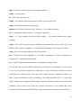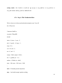
1
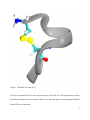
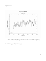
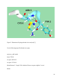
INTERREG IIIA Community Initiative Program
Szegedi Tudományegyetem
Prirodno-matematički fakultet, Univerzitet u Novom Sadu
„Computer-aided Modelling and Simulation in Natural Sciences“
University of Szeged,
Project No. HUSER0602/066
Molecular modeling, Interactions in Biological
Systems I.
Prof. Dr. György Dombi
István Mándity
Contents
1.
Synopsis
2.
Research Problem
3.
Creating the input file
4.
Molecular Dynamics
5.
Analysis
6.
Bibliography
1
1. Synopsis
Today you will learn how to use one of the most versatile molecular mechanics/dynamics
modeling packages, AMBER 9. [1] The AMBER suite of programs was developed by the late
Peter A Kollman and colleagues at the University of California San Francisco (UCSF). The
Amber package was designed with the ability to address a wide variety of biomolecules including
proteins and nucleic acids as well as small molecule drugs. See http://amber.scripps.edu for more
information.
2. Research Problem
We will study the X-ray crystal structure of the oxytocin-neurophysin complex (1NPO.PDB). [2]
We will focus on oxytocin itself. Remember, the X-ray crystal structure has no hydrogen atoms
or lone pairs. The AMBER Leap program will take care of adding hydrogens, etc. When working
with a crystal structure for the first time, you must carefully review the data in the beginning of
the PDB file (REMARKS provide important information!). For example, the structure may be
missing side chains in some of its residues or it may even be missing entire residues! A very
important information item in a PDB file of a protein is the SSBOND records, which designate
all of the disulfide bonds found in the structure. You will need this information for processing
your file in Leap.
2
Figure 1. 3D model of Oxytocin [3]
Note the key disulfide bond in the oxytocin structure to the left. We will use dynamics to study
the impact of mutation on this structure. What do you think the impact of removing this disulfide
bond will be to the structure?
3
3. Creating the input file
Make a project directory and use it for this exercise. Download 1NPO.pdb from the protein data
bank (http://www.rcsb.org). Log in with Putty program to the mangan cluster, create there your
own project library Transfer this file to the mangan cluster with an sftp program. Review the
PDB file in a text editor (nedit, gedit, kedit, etc.).
nedit 1NPO.pdb
You will notice that the structure is a dimer of two complexes. You should also notice that in the
REMARK section we find that REMARK 6 informs us that the first several residues and the last
several residues (86-95) in neurophysin were not found or resolved in the structure. We will
ignore these for now as they are not important. Using your text editor, remove chains A, C, and D
along with any water molecules and ions from the PDB file. We only need one complex! (ATOM
566 ATOM 633) Save your new file as oxyt.pdb.
3.1. Prepare the AMBER coordinate (inpcrd or crd for short) and
topology (prmtop or just top) files
We will use the tLeap program.
Terminal Leap can be used to automate this process. The script below can be used to perform the
file preparation you. The oxy.scr script for tleap:
4
source leaprc.ff03
HOH=SPC
WAT=SPC
loadamberparams frcmod.spce
oxy = loadPdb oxyt.pdb
bond oxy.1.SG oxy.6.SG
check oxy
saveAmberParm oxy oxy_vac.top oxy_vac.crd
solvateOct oxy TIP3PBOX 9.0
saveAmberParm oxy oxy.top oxy.crd
Quit
source leaprc.ff03
HOH=SPC
WAT=SPC
The leaprc.ff03 file loads the parameters for the AMBER03 force field and makes adjustments
for use of the SPC/E water model.
loadamberparams frcmod.spce
Loads the parameters
oxy = loadPdb oxyt.pdb
5
load into the oxy variable the pdb file
bond oxy.1.SG oxy.6.SG
The
bond
command
creates
bonds
between
atoms.
The
syntax
is:
unit_name.residue_number.atom_name. Create the disulfide bond between the two cystein
residues.
check oxy
After using the check command you will notice several warnings about close contacts and
possibly a warning about the overall charge of the unit if the unit is not neutral in overall formal
charge. The overall charge is important, as we must neutralize this charge for particle-mesh
ewald electrostatics later on.
saveAmberParm oxy oxy_vac.top oxy_vac.crd
Save a topology and coordinate file for in vacuo runs.
solvateOct oxy TIP3PBOX 9.0
6
We will use the solvateOct command to solvate the structure in SPC/E water [6] using a
truncated octahedron periodic box. You have told Leap to solvate the unit in a truncated
octahedral box using spacing distance of 9.0 angstroms around the molecule. Ideally, you should
set the spacing at no less than 8.5 Å (~ 3 water layers) to avoid periodicity artifacts. [7] For
particle-mesh ewald electrostatics, [8, 9] our box side length must be > 2 X NB cutoff. We will
use a 10.0 Å cutoff in our solvated system; therefore, our box side must be > 20 Å. Our box side
length will be (2 X 9) + peptide dimension, which should easily be greater than 20 Å. The system
must be neutral in terms of overall formal charge. Fortunately, our system is neutral as is. If this
had not been the case then we would have used the addIons command to neutralize the charge
(use Na+ to counter a negative charge or Cl- to counter a positive charge).
saveAmberParm oxy oxy.top oxy.crd
The saveAmberParm command saves the parameter file (prmtop or top file) and the initial
coordinate file (inpcrd or crd file). We did this before solvating the system so we could perform
an in vacuo dynamics simulation for comparison to the solvated system.
The tleap program is very useful in situations where you might need to process a very large
structure that requires a large solvent box and ions.
You’re done with file preparation (hooray!). You will notice a file called “leap.log” in your
working directory. Leap records every command and result (as well as commands issued by Leap
7
under the hood) in a log file. Some of the information in this log file is required for publication
(e.g. periodic box size; # of water molecules; # of ions if any, etc).
Make a separate directory for your in vacuo dynamics runs and move your oxy_vac.top and
oxy_vac.crd files there.
mkdir in_vacuo
mv oxy_vac.* in_vacuo
cd in_vacuo
4. Molecular Dynamics
4.1. The in vacuo Model
This computation will be performed in two steps using an NVT ensemble. An energy
minimization will be done followed by a production dynamics run.
4.1.1. Step 1. Energy Minimization of the System
We perform a steepest descents energy minimization to relieve bad steric interactions that would
otherwise cause problems with or dynamics runs followed up with conjugate gradient
8
minimization to get closer to an energy minimum. The SANDER program is the number
crunching juggernaut of the AMBER software package. SANDER will perform energy
minimization, dynamics and NMR refinement calculations. You must specify an input file to tell
SANDER what computations you want to perform and how you would like to perform those
computations. Study the input file for energy minimization below.
min_vac.in
oxytocin: initial minimization prior to MD
&cntrl
imin = 1,
maxcyc = 500,
ncyc = 250,
ntb = 0,
igb = 0,
cut = 12
/
Issue the following command to run your in vacuo energy minimization.
subamber9.sh mangan neverend sander –O –i min_vac.in –o min_vac.out –p oxy_vac.top –c
oxy_vac.crd –r oxy_vacmin.rst
9
4.1.2. Step 2. Molecular dynamics
Use the following md_vac.in script.
oxytocin MD invacuo,
12 angstrom cut off, 250 ps
&cntrl
imin = 0, ntb = 0,
igb = 0, ntpr = 100, ntwx = 500,
ntt = 3, gamma_ln = 1.0,
tempi = 300.0, temp0 = 300.0,
nstlim = 125000, dt = 0.002,
cut = 12.0
/
subamber9.sh mangan 1 neverend sander –O –i md_vac.in –o md_vac.out –p oxy_vac.top –c
oxy_vacmin.rst –r oxy_vacmd.rst –x oxy_vacmd.mdcrd –ref oxy_vacmin.rst –inf mdvac.info
There are many more settings/flags above than we can possibly explain here. So, for more in
depth info please consults the AMBER User’s Manual.
The settings important for minimization are highlighted and explained below.
10
&cntrl and / – Most if not all of your instructions must appear in the “control” block
(hence&cntrl).
cut = nonbonded cutoff in angstroms.
ntr = Flag used to perform position restraints (1 = on, 0 = off)
imin = Flag to run energy minimization (if = 1 then perform minimization; if = 0 then perform
molecular dynamics).
maxcyc = maximum # of cycles
ncyc = After ncyc cycles the minimization method will switch from steepest descents to
conjugate gradient.
ntmin = Flag for minimization method. (if = 0 then perform full conjugate gradient min with the
first 10 cycles being steepest descent and every nonbonded pairlist update; if = 1 for ncyc cycles
steepest descent is used then conjugate gradient is switched on [default]; if = 2 then only use
steepest descent)
dx0 = The initial step length
dxm = The maximum step allowed
drms = gradient convergence criterion 1.0E4 kcal/mol•Å is the default
4.2. Molecular Dynamics in a Water Box
This job will be accomplished in 4 steps:
Step 1. Restrained Minimization – relieve bad vander Waals contacts in the surrounding solvent
while keeping the solute (protein) restrained.
Step 2. Unrestrained Minimization – Relieve bad contacts in the entire system.
11
Step 3. Restrained Dynamics – Relax the solvent layers around the solute while gradually
bringing the system temperature from 0 K to 300 K.
Step 4. Production Run – Run the production dynamics at 300 K and 1 bar pressure.
******************
4.2.1. Step 1. Restrained Minimization
oxytocin: initial minimisation solvent + ions
&cntrl
imin = 1,
maxcyc = 1000,
ncyc = 500,
ntb = 1,
ntr = 1,
cut = 10
/
Hold the protein fixed
500.0
RES 1 9
END
END
Hold the peptide fixed
500.0 (This is the force in kcal/mol used to restrain the atom positions.)
RES 1 9 (Tells AMBER to apply this force to residue #’s 1 to 9).
12
4.2.2. Step 2. Unrestrained Minimization
oxytocin: initial minimisation whole system
&cntrl
imin = 1,
maxcyc = 2500,
ncyc = 1000,
ntb = 1,
ntr = 0,
cut = 10
/
4.2.3. Step 3. Position Restrained Dynamics
This initial dynamics run is performed to relax the positions of the solvent molecules. In this
dynamics run, we will keep the macromolecule atom positions restrained (not fixed, however). In
a position restrained run, we apply a force to the specified atoms to minimize their movement
during the dynamics. The solvent we are using in our system, water, has a relaxation time of 10
ps; therefore we need to perform at least > 10 ps of position restrained dynamics to relax the
water in our periodic box.
Contents of md1.in
oxytocin: 25ps MD with res on protein
13
&cntrl
imin = 0,
irest = 0,
ntx = 1,
ntb = 1,
cut = 10,
ntr = 1,
ntc = 2,
ntf = 2,
tempi = 0.0,
temp0 = 300.0,
ntt = 3,
gamma_ln = 1.0,
nstlim = 12500, dt = 0.002,
ntpr = 100, ntwx = 500, ntwr = 1000
/
Keep protein fixed with weak restraints
10.0
RES 1 9
END
END
ntb = 1 Constant volume dynamics.
14
imin = 0 Switch to indicate that we are running a dynamics.
nstlim = # of steps limit.
dt = 0.002 time step in ps (2 fs)
temp0 = 300 reference temp (in degrees K) at which system is to be kept.
tempi = 100 initial temperature (in degrees K)
gamma_ln = 1 collision frequency in ps 1 when ntt = 3 (see Amber 8 manual).
ntt = 3 temperature scaling switch (3 = use langevin dynamics)
tautp = 0.1 Time constant for the heat bath (default = 1.0) smaller constant gives tighter
coupling.
vlimit = 20.0 used to avoid occasional instability in dynamics runs (velocity limit; 20.0 is the
default). If any velocity component is > vlimit, then the component will be reduced to vlimit.
comp = 44.6 unit of compressibility for the solvent (H2O)
ntc = 2 Flag for the Shake algorithm (1 – No Shake is performed; 2 – bonds to hydrogen are
constrained; 3 – all bonds are constrained).
tol = #.##### relative geometric tolerance for coordinate resetting in shake.
You will note that we used a smaller restraint force (10 kcal/mol). For dynamics, one only needs
to use 5 to 10 kcal/mol restraint force when ntr = 1 (uses a harmonic potential to restrain
coordinates to a reference frame; hence, the need to include reference coordinates with the –ref
flag.). Larger restraint forces lead to instability in the shake algorithm with a 2 fs time step.
Larger restraint force constants lead to higher frequency vibrations, which in turn lead to the
instability. Excess motion away from the reference coordinates is not possible due to the
steepness of the harmonic potential. Therefore, large restraint force constants are not necessary.
15
nohup sander –O –i md1.in –o md1.out –p oxy.top –c oxy_min2.rst –r oxy_md1.rst –x
oxy_md1.mdcrd –ref oxy_min2.rst –inf md1.info
4.2.4. Step 4. The Production Run
This is where we do the actual molecular dynamics run. You will
do a 250 ps run.
Contents of md2.in
oxytocin: 250ps MD
&cntrl
imin = 0, irest = 1, ntx = 5,
ntb = 2, pres0 = 1.0, ntp = 1,
taup = 2.0,
cut = 10, ntr = 0,
ntc = 2, ntf = 2,
tempi = 300.0, temp0 = 300.0,
ntt = 3, gamma_ln = 1.0,
nstlim = 125000, dt = 0.002,
ntpr = 100, ntwx = 500, ntwr = 1000
/
ntb = 2 Constant pressure dynamics.
ntp = 1 md with isotropic position scaling.
16
taup = 2.0 pressure relaxation time in ps
pres0 = 1 reference pressure in bar.
Issue the following command to run your dynamics simulation.
subamber9.sh mangan 1 neverend sander –O –i md2.in –o md2.out –p oxy.top –c oxy_md1.rst – r
oxy_md2.rst –x met_md.mdcrd –ref oxy_md1.rst –inf md2.info
5.
Analysis
5.1. The potential energy fluctuation throughout the simulation
Copy process_mdout.perl to your working project directory.
./process_mdout.perl md1.out md2.out
The resulting files are readable as space delimited files in Excel. Read the summary.EPTOT
(potential energy plot) file. The potential energy fluctuates throughout the simulation. There is a
jump in energy early on during the water equilibration (restrained MD in the first 25 ps) phase
followed by a general trend toward lower energy, which is a good sign that the dynamics is
leading toward lower energy conformations. Plot other files. Use Microsoft Excel to read in the
file as a space delimited file
summary.TEMP gives the temperature fluctuation with time.
17
summary.PRES gives the pressure fluctuation with time.
5.2. The RMS plot
We will use the ptraj program.
Contents of rms.in
trajin oxy_md1.mdcrd
trajin oxy_md2.mdcrd
rms first out oxy.rms @N,C,CA time 1.0
trajin – specifies trajectory file to process
rms – computed RMS fit to the first structure of the first trajectory read in.
out – specifies name of output file
@N, C, CA – Atom mask specifier (backbone atoms) (Note: The @ symbol is the atom specifier;
alternately or in combination, you may use the colon : to specify residue ID # aswell) For
example if you only desired to examine the backbone atoms of residue #23, use :23@N,C,CA
time – tells ptraj that each frame represents 1 ps
Issue the following command to run ptraj.
ptraj oxy.top < rms.in
18
xmgrace oxy.rms
5.3. Analysis of hydrogen bonds over the course of the trajectory
Use the following input file (hbond.in) to ptraj.
19
Figure 2. Illustration of hydrogen bonds to be analyzed [3]
Use the following input file (hbond.in) to ptraj.
trajin oxy_md2.mdcrd
donor TYR O
acceptor ASN N H
acceptor CYX N H
hbond distance 3.5 angle 120.0 includeself donor acceptor neighbor 2 series \
hbond
20
DONOR/ACCEPTOR – use to specify the donor and acceptor atom in the H-bond.
DISTANCE – use to specify the cutoff distance in angstroms between the heavy atoms
participating in the interaction. (3.0 is the default)
INCLUDESELF – include intramolecular Hbond interactions if any.
ANGLE – The Hbondangle cutoff (Hdonoracceptor) in degrees. (0 is the default)
SERIES – Directs output of Hbond
data summary to STDOUT.
ptraj oxy.top < hbond.in > hbond.dat
The statistical analysis in the hbond.dat file will be most important. Look for those Hbonds with a
high % occupancy (> 60%). These are the more stable Hbonds.
Throw out results with angles less than 120 degrees. The higher the % occupancy; the better.
When analyzing Hbond data, it is best to establish reasonable guidelines for the distance and
angle cutoffs. A recent paper by Chapman et al. provides a nice discussion of hydrogen bond
criteria. [10]
5.4. Torsion angle measurements of the peptide backbone
Use the following input file (torsion.in) to ptraj.
trajin oxy_md2.mdcrd
dihedral phi_1 :1@C :2@N :2@CA :2@C out phi_1
21
dihedral psi_1 :1@N :1@CA :1@C :2@N out psi_1
dihedral omega_1 :1@CA :1@C :2@N :2@CA out omega_1
dihedral phi_2 :2@C :3@N :3@CA :3@C out phi_2
dihedral psi_2 :2@N :2@CA :2@C :3@N out psi_2
dihedral omega_2 :2@CA :2@C :3@N :3@CA out omega_2
dihedral phi_3 :3@C :4@N :4@CA :4@C out phi_3
dihedral psi_3 :3@N :3@CA :3@C :4@N out psi_3
dihedral omega_3 :3@CA :3@C :4@N :4@CA out omega_3
dihedral phi_4 :4@C :5@N :5@CA :5@C out phi_4
dihedral psi_4 :4@N :4@CA :4@C :5@N out psi_4
dihedral omega_4 :4@CA :4@C :5@N :5@CA out omega_4
dihedral phi_5 :5@C :6@N :6@CA :6@C out phi_5
dihedral psi_5 :5@N :5@CA :5@C :6@N out psi_5
dihedral omega_5 :5@CA :5@C :6@N :6@CA out omega_5
ptraj oxy.top < torsions.in
The individual files can be plotted withMicrosoft Excel to view the dihedral angle fluctuation
with time in the simulation.
5.5. How to view a trajectory movie with VMD
A viewer utility that you may use on various platforms to view Amber coordinate files and
22
trajectory files is Visual Molecular Dynamics (VMD; see http://www.ks.uiuc.edu/Research/vmd/
). [3]
VMD Main: File > New Molecule > Molecule File Browser > Filename: Click on Browse… >
Choose a molecule file: oxy.top > Click OK
Molecule File Browser > Determine file type: parm7 > Click on Load
Keep the Molecule File Browser window open!
Molecule File Browser > Filename: Click on Browse… > Choose a molecule file:
oxy_md2.mdcrd > Click OK
Molecule File Browser > Determine file type: crdbox > Click on Load
You will notice lots of water molecules. Use Graphics Representations to view just the protein.
VMD Main: Graphics > Representations > Graphical Representations > Selected Atoms: protein
Click Apply
Use the left mouse button for xy rotation and the middle mouse button for z rotation. Hit the s
key on your keyboard and the mouse goes into scale (zoom in and out) mode. Hit the t button and
the mouse will be in translation mode. Hit the r button to return to rotation mode. [12]
6.
Bibliography
1. Case, D.A., T.E. Cheatham III, T. Darden, H. Gohlke, H. Luo, K.M. Merz, A. Onufriev,
C. Simmerling, B. Wang, and R. Woods, The Amber biomolecular simulation programs.
J. Comput. Chem., 2005. 26: p. 16681688.
2. Rose, J., C. Wu, C. Hsiao, E. Breslow, and B. Wang, Crystal structure of the
neurophysinoxytocin complex. Nature Struct. Biol., 1996. 3(2): p. 163169.
23
3. Humphrey, W., A. Dalke, and K. Schulten, VMD Visual Molecular Dynamics. J. Molec.
Graphics, 1996. 14.1: p. 3338.
4. Merritt, E.A. and D.J. Bacon, Raster3D: Photorealistic Molecular Graphics. Methods
Enzymol., 1997. 277: p. 505524.
5. Duan, Y., C. Wu, S. Chowdhury, M. Lee, G. Xiong, W. Zhang, R. Yang, P. Cieplak, R.
Luo, T. Lee, J. Caldwell, J. Wang, and P. Kollman, A pointcharge force field for molecular
mechanics simulations of proteins based on condensedphase quantum
mechanical calculations. J. Comput. Chem., 2003. 24(16): p. 19992012.
6. Berendsen, H.J., J. Grigera, and T. Straatsma, The missing term in effective pair
potentials. J. Phys. Chem., 1987. 91: p. 62696271.
7. Weber, W., P.H. Hünenberger, and J.A. McCammon, Molecular Dynamics Simulations of a
Polyalanine Octapeptide under Ewald Boundary Conditions: Influence of Artificial Periodicity
on Peptide Conformation. J. Phys. Chem. B, 2000. 104(15): p. 36683575.
8. Darden, T., D. York, and L. Pedersen, Particle Mesh Ewald: An Nlog(N) method for Ewald
sums in large systems. J. Chem. Phys., 1993. 98: p. 1008910092.
9. Essmann, U., L. Perera, M.L. Berkowitz, T. Darden, H. Lee, and L. Pedersen, A smooth
particle-mesh ewald potential. J. Chem. Phys., 1995. 103: p. 85778592.
10. Fabiola, F., R. Bertram, A. Korostelev, and M.S. Chapman, An Improved Hydrogen Bond
Potential: Impact on Medium Resolution Protein Structures. Protein Sci., 2002. 11: p. 14151423.
11. Lindahl, E., B. Hess, and D. van der Spoel, GROMACS 3.0: a package for molecular
simulation and trajectory analysis. J. Mol. Model, 2001. 7: p. 306317.
12. Kerrigan J., E. AMBER 9.0 Introductory Tutorial
24