Download Solution Optimizer - Universal Technical Systems

This excerpt is taken from the TK Solver 5.0 User Manual to give you a better idea of how the Solution
Optimizer can help you accomplish more in less time. The solution Optimizer, included in the TK Solver
5.0 Premium Edition, is a valuable tool that gives you advanced control over constraints and bounds to
help you achieve optimal design parameters—no programming required! You’ll like the easy–to–use,
Wizard–driven system that readily walks you through the process and empowers you to take your design
to a whole new level! See what the Solution Optimizer can do for you today!
TK Solver 5.0
User’s Guide
Universal Technical Systems, Inc.
Credits Page
Copyright
The UTS documentation and the software are copyrighted with all rights reserved. Under the copyright laws, neither the documentation nor the software may be
copied, photocopied, reproduced, translated, or reduced to any electronic or machine readable form, in whole or part, without the prior written consent of UTS.
Copyright  1983-2013 Universal Technical Systems, Inc.
Universal Technical Systems, Inc.
4053 North Perryville Road, Loves Park, Illinois 61111
Phone (815) 963-2220 Fax (815) 963-8884
All rights reserved. First edition printed in August 1994 in the U.S.A. Revised 2004.
Contains images by Corel Corp., 1600 Carling Ave., Ottawa, Ontario, Canada K1Z 8R7, (613) 728-3733.
Contains Macromedia Flash™ Player software by Macromedia, Inc., Copyright © 1995-1999 Macromedia, Inc. All rights reserved.
Macromedia and Flash are trademarks of Macromedia, Inc.
Contains Macromedia Shockwave™ Player software by Macromedia, Inc., Copyright © 1995-1999 Macromedia, Inc. All rights reserved.
Macromedia and Shockwave are trademarks of Macromedia, Inc."
Trademarks
Following is a list of Trademarks™ or Registered Trademarks® and the companies by which they are owned:
TK Solver for Windows, TK Solver, TK, TK Solver Plus, TK Plus, TK!Solver, Roark & Young Demo, MiniTK, Roark & Young on TK,
Heat Transfer on TK, Dynamics & Vibration Analysis, Gear Analysis Software, DesignLink, Queueing Analyses, Tolerance Analysis,
TK/CAD Link and MathLook by Universal Technical Systems, Inc.
Windows, Word, Excel, and Visual Basic by Microsoft Corporation.
Limitation of Liability
Universal Technical Systems, Inc. (UTS) does not warrant that the software program will function properly in every hardware/software
environment. The software may not work in combination with modified versions of the operating system, with certain print-spooling or
file facility programs or with certain printers supplied by independent manufacturers.
Although UTS has tested the software and reviewed the documentation, UTS makes no warranty or representation either expressed or
implied, with respect to this software or documentation, including their quality, performance, merchantability, or fitness for a particular
purpose. As a result, this software and documentation are licensed “as is” and you, the licensee, are assuming the entire risk as to their
quality and performance.
In no event will UTS be held liable for direct, indirect, special, incidental, or consequential damages arising out of the use or inability to use
the software or documentation, even if advised of the possibility of such damages. In particular, UTS is not responsible for any costs
including but not limited to those incurred as a result of lost profits or revenue, loss of use of the computer program, loss of data, the cost
of substitute programs, claims by third parties or for other similar costs.
TK5-090904
Solution Optimizer
7
Solution Optimizer is included with the Premium version of TK Solver. If you do not have this
feature and would like to order it, please call UTS at 815-963-2220.
The purpose of the Optimizer is to find the set of input values that would provide the preferred
solution to the current model. The user can set preference criteria and limitations to be imposed in the
search. The Optimizer can help solve linear, nonlinear, and integer programming problems. It can also
be used as an alternative to TK Solver’s built-in Iterative Solver for solving systems of equations. In
this use the Optimizer offers more control over constraints and bounds on variables.
The Optimizer acts like a shell around a TK Solver model. It calls the model repeatedly, starting with
the current values, until the constraints are satisfied or the process fails. It is important to distinguish
the Optimizer from TK functions. You cannot include a rule on the Rule Sheet to activate the
optimizer. TK does not call the Optimizer. The reverse is actually true: the entire TK model acts like a
subroutine called by the Optimizer.
The Optimizer requires that the underlying TK model be solvable without error conditions over the
domain of the variables in the optimization. If a TK error is triggered, the Optimizer is halted and the
error message is displayed. Additional bounds can be added to prevent such errors. After such an
error, the Optimizer must be restarted. It does not continue on from the point of the error.
It is recommended that a model be tested before running the Optimizer on it. Such testing would
automatically cause the outputs (or error messages) to appear.
Any TK Solver model can be used with the Optimizer. There is no special programming required.
The Optimizer works with the existing variables and lists. This means that all the TK models from the
many TK-based applications can be optimized.
Here are the steps required for using the Optimizer:
1.
2.
3.
Build a TK model that solves over the required domain.
Set up the optimization constraints and bounds using either the Set Up Optimizer Command
or the Optimizer Wizard.
Press F11 to launch the Optimizer.
7-1
Part 2—Equation Solving
Optimize What?
An optimizer is a software tool that help users find the best way to design components or allocate
scarce resources. The resources may be raw materials, machine time or people time, money, or
anything else in limited supply. The “best” or optimal solution may be maximizing profits, minimizing
costs, or achieving the best possible quality. An almost infinite variety of problems can be tackled this
way.
The Optimizer significantly broadens the domain of problems you can solve with TK. Students and
professionals in all areas of science, engineering, finance, operations research and management will
find this to be a valuable, time-saving tool. Here are a few problems TK can now tackle with ease.
Finance and Investment
Working capital management involves allocating cash to different purposes (accounts receivable,
inventory, etc.) across multiple time periods, to maximize interest earnings.
Capital budgeting involves allocating funds to projects that initially consume cash but later generate
cash, to maximize a firm’s return on capital.
Portfolio optimization –creating “efficient portfolios” – involves allocating funds to stocks or bonds
to maximize return for a given level of risk, or to minimize risk for a target rate of return.
Manufacturing
Job shop scheduling involves allocating time for work orders on different types of production
equipment, to minimize delivery time or maximize equipment utilization.
Blending (of petroleum products, ores, animal feed, etc.) involves allocating and combining raw
materials of different types and grades, to meet demand while minimizing costs.
Cutting stock (for lumber, paper, etc.) involves allocating space on large sheets or timbers to be cut
into smaller pieces, to meet demand while minimizing waste.
7-2
Chapter 7—Solution Optimizer
Distribution and Networks
Routing (of goods, natural gas, electricity, digital data, etc.) involves allocating something to different
paths through which it can move to various destinations, to minimize costs or maximize throughput.
Loading (of trucks, rail cars, etc.) involves allocating space in vehicles to items of different sizes so as
to minimize wasted or unused space.
Scheduling of everything from workers to vehicles and meeting rooms involves allocating capacity to
various tasks in order to meet demand while minimizing overall costs.
Anything you can think of modeling with TK Solver is now fair game for the Optimizer. Just enter
some equations and you’re ready to go!
Here are two examples, followed by a summary of the commands and features, and three case studies
for additional practice.
7-3
Part 2—Equation Solving
1 - Trivial Example
A simple example, with known solution, illustrates the basics
of this tool. We will find the rectangular quadrilateral of
largest area that can be inscribed in a circle of fixed radius.
We begin by modeling the situation for a sample radius of
unit value.
A model of this situation might be the following:
We can see that assigning different input values to the angle alpha gives different solutions for the
variable area. Our goal is to find the value of alpha that results in the maximum value of area.
The Optimizer first searches the Variable Sheet for outputs and provides a list of variables that can be
declared as the target variable. If the model has not been solved and no outputs are displayed, the
Optimizer will not display any target variable options. In this example, the target variable is area.
7-4
Chapter 7—Solution Optimizer
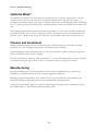
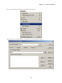
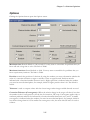
We open the Optimizer. Clicking Commands Setup Optimizer…
The parameters for the optimization can then be set in the panel that opens:
7-5
Part 2—Equation Solving
Select the target variable and the variable(s) that the Optimizer will modify (the decision variables)
by using the selection (…) buttons1. We will set the value of “Equal To:” to “Maximize” (the default).
No constraints are required for this problem.
Clicking the “Optimize” button causes the model to solve repeatedly under control of the Optimizer,
which modifies alpha each run until area reaches a maximum, 2, at the angle 45 (degrees) as
expected.
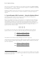
2 – Typical Example, With Constraints – Using the Optimizer Wizard
The following problem is taken from Basic Programs for Production and Operation Management by
Pantumsinchai, Hassan, and Gupta (Prentice-Hall, 1983).
Butane, Virgin Naphtha and Catalytic Cracked Gasoline are to be blended into Super and Regular
unleaded gasoline. The goal is to blend the components so as to produce the two types of gasoline
with a maximum profit. There are six unknowns, corresponding with the daily consumption of
components used for each kind of gasoline. This can be represented by two equations, with TS and
TR representing the total units of Super and Regular produced. For example, the variable x11
represents the units of Butane in Super.
TS = x11 + x21 + x31
TR= x12 + x22 + x32
For any blend, the octane rating can be computed for Super and Regular using the following
equations, with OCT1, OCT2, and OCT3, the octane rating values of the three components.
OCTS=
OCT1 x11 + OCT2 x21 + OCT3 x31
TS
OCTR=
OCT1 x12 + OCT2 x22 + OCT3 x32
TR
The minimum octane numbers for Super and Regular are 92 and 87 respectively.
Another important criterion of the blends is the Reid Vapor Pressure (RVP). The following equations
are used to compute the RVP for Super and Regular, with RVP1, RVP2, and RVP3 the values from
each of the components.
RVPS =
RVP1 x11 + RVP2 x21 + RVP3 x31
TS
RVPR =
RVP1 x12 + RVP2 x22 + RVP3 x32
TR
If you do not see the target you had in mind, or if you cannot select the variables you want to adjust,
re-check in the Variable Sheet to be certain the target variable has an output value and the variables to
be adjusted have input values.
1
7-6
Chapter 7—Solution Optimizer
The maximum for both RVPS and RVPR is 8.
There are limitations on the availability of each of the components. The equations for the total of each
component used are as follows.
A1 = x11 + x12
A2 = x21 + x22
A3 = x31 + x32
This will allow us to compare A1, A2, and A3 with the available amounts.
The last equation defines the total profit from both blends, where p1 and p2 are the profits per unit
of production of Super and Regular, respectively.
F = p1 TS + p2 TR
7-7
Part 2—Equation Solving
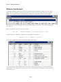
These equations can be entered into TK Solver to establish the objective function for the
optimization. The TK Solver Variable Sheet is shown next.
With inputs provided for each component and with values of 1 input for each of the six sample
quantities, we see the results at the bottom of the sheet. Our goal is to determine the values of these
six quantities that produce a maximum value for F and which satisfy the vapor pressure and octane
rating requirements for the blends. To accomplish this, we can use the TK Optimizer.
7-8
Chapter 7—Solution Optimizer
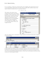
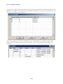
We launch the Optimizer Wizard and define the target variable and constraints.






Total profit, F, is selected as the objective variable (the same as a target variable).
Quantities x11, x21, x31, x12, x22, and x32 are identified as decision
variables with minimal values set to 0.
Constraints are placed on the octane rating of Super and Regular, variables OCTS and OCTR,
to be a minimum of 92 and 87, respectively.
Constraints are placed on the resulting vapor pressures of both the Super and Octane blends.
In this case, the maximums are 8 for both.
Constraints are placed on the available units of each of the three components. 25 units of
Butane, 40 units of Virgin Naphtha, and 100 units of C/C Gasoline.
Constraints are added to indicate that at least some Super and some Regular must be
produced. That is, x11 + x21 + x31 => 0.1 and
x12 + x22 + x32 => 0.1.
The Optimization Wizard screens are shown on the following pages, along with the optimal solution.
7-9
Part 2—Equation Solving
7-10
Chapter 7—Solution Optimizer
Clicking the “Finished” button produces the solution quickly, displayed on the TK Variable Sheet.
7-11
Part 2—Equation Solving
Setting Up the Optimizer
The Optimizer is based on the widely used Solver technology from Frontline Systems. If you are
familiar with Microsoft Excel, you might know that it includes a version of Frontline’s Solver as an
add-in, and you may have become comfortable with that interface to Solver. TK includes two
different approaches to setting up the Optimizer. One is very similar to the Excel Solver approach, so
Excel users feel comfortable right away. We also include a second approach, via a TK Solver Wizard,
which we hope is easier to use for those of you who might be new to the concept.
The TK Solver Commands menu includes two selections related to the Optimizer.
“Setup Optimizer…”—This starts the configuration process, which can culminate with running the
Optimizer or saving the settings for later. The interface is similar to that used for configuring the
Excel Solver.
7-12
Chapter 7—Solution Optimizer
“Run Optimizer”—This runs the Optimizer with the values last selected, using current Variable Sheet
inputs as initial guesses. It is equivalent to using “Setup Optimizer…” without changing anything. The
keystroke shortcut is F11.
The Optimizer works with several different types of variables and it is important to note how it
interacts with them.
The Target Variable is the TK variable that you want to maximize, minimize, or set equal to a value.
Any TK variable that does not have an input value can be set as the target variable. A target variable is
sometimes referred to as a dependent variable or an objective variable.
The target can be any valid TK expression that produces a numeric value. If the target value in a TK
model is actually the element of a list, you can create a rule equating the list element with a variable
before using the Optimizer. For example, if you want to use the 100 th element of the list named
temperature as your target value, you could create the following rule on the Rule Sheet and use
variable tn as your target variable.
tn = 'temperature[100]
Change Variables are those variables that you want the Optimizer to try changing in order to achieve
your goal for the target variable. A change variable must be an input variable in the TK model. It
cannot have a guess status. Change variables are sometimes called decision variables or
independent variables.
7-13
Part 2—Equation Solving
If a change value of interest in a TK model is actually a list element, you must create a rule placing the
value of a variable from the Variable Sheet into the list element before using the Optimizer. For
example, if the 4th element of the list named depth should be changed in the optimization process, the
following rule assigns the value of the variable named D to the list element and the Optimizer uses D
as a change variable.
Place('depth,4) = D
It is very important that you not use a TK variable with a guess status for a target value when
you launch the Optimizer. A guess value will only be used by the Optimizer on its first pass through
the TK model and will not be available on subsequent passes. If a guess value is required in the model,
use a first guess on the variable subsheet; that guess will be triggered automatically on each pass. Such
a variable could be used as the target variable by the Optimizer.
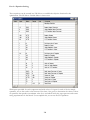
Available Variables
Whenever you see the ellipsis button
you may click on it for a list of variables to add to the
current field. The variables listed will meet the required criteria. For example, if you click on the
ellipsis button for the Target Variable, you will be shown a list of variables with output status on the
TK Variable Sheet. Likewise, the ellipsis button for the change variables produces a list of variables
that have inputs.
Bounds and Constraints
Bounds are limits beyond which the Optimizer should not search. Constraints are limitations set on
the end result, but the Optimizer may search beyond them in finding the optimal solution. In other
words, it may be necessary for the Optimizer to get a bigger picture of the problem to better solve it.
Because of this important difference, bounds and constraints are handled separately in the interface.
It is possible to set bounds for variables that may cause an error condition. For example, if you know
that the model fails if the value of T exceeds 100, and T is one of your change variables, you can set
an upper bound on T. You can also set bounds that are functions of existing variables and
expressions, but it is very important to note that these bounds are set based on the initial conditions of
the model and do not dynamically update as the model is repeatedly solved. Bounds should be
numeric values or expressions involving only input variables or list elements that will not change in the
solution process. For example, you might set a bound that Di must be less than Do, restricting an
inner diameter to be less than an outer diameter. This allows you to change the input for Do and rerun
the optimization without having to use the commands menu to change the bounds.
Optimizer can violate the bounds but will only do so as a last resort if it is unable to find its way to a
solution within the bounds.
7-14
Chapter 7—Solution Optimizer
Constraints can look exactly the same as bounds, but constraints are repeatedly updated and checked,
and they can be temporarily violated during the course of the optimization process. For example, if
you have a variable p whose result should not be more than 80% of pcrit, you can set a constraint,
p <= 0.8*pcrit, and the Optimizer will use that as a guide. At times during the process, p might
exceed the limit, but the Optimizer will not finish until the constraint is satisfied. When all the
constraints are true and the Optimizer fails to improve on the target condition, the Optimizer is
finished and the results are posted.
Adding Constraints
Clicking the Add button opens the Add/Edit Constraint dialog for entry of constraints. Any valid TK
expressions are allowed. This dialog will also appear if you double-click on any existing constraints in
the Optimization Parameters window. In that case, the constraint will be displayed and the contents
can be edited. An alternative to double-clicking on a constraint is to highlight the constraint and click
the Change button. To remove a constraint, highlight it and click the Delete button.
After the expressions have been entered in the Add/Edit Constraint dialog, click the Add button to
add another constraint or the OK button to close the dialog and return to the Optimization
Parameters window. The Cancel button cancels any edits and returns to the main window.
7-15
Part 2—Equation Solving
Adding Bounds
To add bounds on any change variables, click the Bounds button. This opens the Bounded Variables
dialog. By default, all the change variables are listed without bounds and declared as continuous type
variables. Other Type options are Integer and Binary; you can change the type to either of those by
entering an “i” or a “b” in that column. Integer variables can only take on integer values. Binary
variables can only be 0 or 1. Bounds can be expressions based on other inputs in the model. If t must
be greater than Tcrit, then Tcrit can be assigned as the lower bound. You should not use change
variables as bounds for other change variables. The bound values are only evaluated at the beginning
of the optimization process.
Optimize
The Optimize… button launches the Optimizer. This can also be done using function key F11. It may
be useful to return to the Variable Sheet before launching the Optimizer so you can watch the action.
7-16
Chapter 7—Solution Optimizer
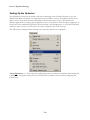
Options
Clicking the Options button opens the Options screen.
Maximum time allowed defaults to 100 seconds. You may want to extend this for problems that you
know will take a long time to solve. The limit is 32000.
Maximum iterations allowed defaults to 1000. You may want to extend this for problems that you
know require many iterations. The limit is 32000.
Precision controls the precision of solutions by using the number you enter to determine whether the
value of a constraint cell meets a target or satisfies a lower or upper bound. Precision must be
indicated with a fractional number between 0 and 1. Higher precision is indicated when the number
you enter has more decimal places; for example, 0.0001 is higher precision than 0.01. The default is
0.0001.
Tolerance is used to compare values with the closest integer when integer variable bounds are used.
Constraint Tolerance (Convergence)—When the relative change in the target cell value is less than
the number in the Convergence box for the last five iterations, TK stops. Convergence applies only to
nonlinear problems and must be indicated by a fractional number between 0 (zero) and 1. A smaller
convergence is indicated when the number you enter has more decimal places; for example, 0.0001 is
less relative change than 0.01. The smaller the convergence value, the more time TK takes to reach a
solution.
7-17
Part 2—Equation Solving
Assume Non-Negative is an option you may want to use frequently. It saves you the trouble of
setting bounds and/or constraints on all variables that you want to assume are greater than or equal to
zero.
Use Automatic Scaling —Select this to use automatic scaling when inputs and outputs have large
differences in magnitude.
Estimates—This specifies the approach used to obtain initial estimates of the basic variables in each
one-dimensional search. The Tangent option uses linear extrapolation from a tangent vector. Quadratic
uses quadratic extrapolation, which can improve the results for highly nonlinear problems.
Derivatives —This specifies the differencing used to estimate partial derivatives of the objective and
constraint functions. Use the Forward option for most problems, in which the constraint values change
relatively slowly. Central should be used for problems in which the constraints change rapidly,
especially near the limits. Although this option requires more calculations, it might help when TK
returns a message that it could not improve the solution.
Search —This specifies the algorithm that is used at each iteration to determine the direction to
search. Newton uses a quasi-Newton method that typically requires more memory but fewer iterations
than the Conjugate gradient method. Conjugate requires less memory than the Newton method but
typically needs more iterations to reach a particular level of accuracy. Use this option when you have a
large problem and memory usage is a concern, or when stepping through iterations reveals slow
progress.
Units and the Optimizer
The Optimizer works with variables in their calculation units. This is done to be consistent with the
rules on the rule sheet and makes TK-based reports easier to understand. It also means that users can
subsequently change the display units for any variables without worrying about affecting any
Optimizer settings.
You may want to set all the variables directly involved in the optimization to their calculation units
before initially setting the optimization constraints and bounds. This will make it easier to make your
optimization entries and to compare values with the bounds and constraints. Use the Properties
dialog to quickly view the calculation units for each variable of interest.
Users of existing TK models should be careful in preparing new Optimization settings, just as they
must be careful when adding new rules to a model. In both situations, it is vital that the calculations
are done in consistent units.
7-18
Chapter 7—Solution Optimizer
Units and Improved Performance and Accuracy
You can use units and conversions to improve the performance of the Optimizer. Try to use display
units that cause values of variables to be relatively close to 1. Since the default precision and
comparison tolerance values are around 1E-6, it can be helpful to try to keep absolute values between
1E-6 and 1E6 but closer to 1 is always better. If the target variables, the change variables or any of the
variables involved in the constraints are relatively small or relatively large, it might be causing the
Optimizer to work harder to reach a solution. On rare occasions, the Optimizer might even
“overlook” the solution altogether.
Using the pressure units example above, it’s possible that your equations are given in units of Pa. The
resulting pcrit value would be 60000000 Pa. By converting to MPa, the pcrit value becomes 60
and the Optimizer can work with it more efficiently.
For more on computational accuracy, see the Technical Time Out starting on page 5-13.
7-19
Part 2—Equation Solving
Optimization with Lists and Tables
TK Solver includes a flexible programming language for processing lists and matrices. Values in lists
can be used as inputs or outputs in optimization problems by mapping them with variables on the
Variable Sheet.
Change Variables
A change variable used in an optimization process can be placed into a list using the PLACE function.
For example, the following rule can be used to place the value of the variable named throttle into
the 10th element of the list named xyz.
PLACE('xyz,10) = throttle
Target Variables
A target variable can receive a value from a list directly on the Rule Sheet. The rule below sets the
value of the variable T equal to the value of the nth element of the list abc.
T = 'abc[n]
It is important to note the difference between referencing list elements in this way and using the
PLACE function. Both are one-way processes, but in opposite directions.
Constraints
Constraints can reference list elements directly. For example, you can add a constraint that specifies
that the 4th element of the list r must be greater than or equal to 0.3.
7-20
Chapter 7—Solution Optimizer
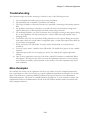
Troubleshooting
The Optimizer might stop before reaching a solution for any of the following reasons:
1.
2.
3.
You interrupted the solution process by pressing Ctrl-Break.
The maximum time or number of iterations was reached.
The Target Variable or Objective Function you specified is increasing or decreasing without
limit.
4. For problems with integer constraints, you need to decrease the Tolerance setting in the
Options dialog box so that Optimizer can find a better integer solution.
5. For nonlinear problems, you need to decrease the Convergence setting in the Options dialog
box so that Optimizer can keep searching for a solution when the target variable value is
changing slowly.
6. You need to select the Use Automatic Scaling check box in the Options dialog box because
some input values are several orders of magnitude apart, or input and output values differ by
several orders of magnitude.
7. Errors occurred in the TK model. You may need to add bounds to avoid such error
conditions.
8. You used “guess status” variables in the TK model. Use default first guesses on the variable
subsheet.
9. Optimizer reports that it is converging too slowly. Try reducing the required precision
settings.
10. One or more expressions result in 0/0 divisions, which TK interprets as undefined. When
this happens, TK skips the rule. This can cause the optimization process to lose continuity
and to behave erratically. Add constraints to the model to force the Optimizer away from
such conditions.
More Examples
We conclude this section on the Optimizer with four case studies. The first example demonstrates
how to minimize cost. The second solves a portfolio optimization problem involving the use of data
tables. The third solves a relatively difficult problem involving the solution of two simultaneous
differential equations. The fourth is a simpler problem showing how to store solutions in tables. The
Optimization folder in the Mathematics section of the TK Library includes models associated with
these examples and more.
7-21
Part 2—Equation Solving
Minimize Cost Example
A company produces rubber used for tires by combining three ingredients: rubber, oil, and carbon
black. The cost of rubber is 0.04 per pound. The cost of oil is 0.01 per pound. The cost of carbon
black is 0.07 per pound. Here are the equations relating the composition with its characteristics.
The hardness must be between 25 and 35, the elasticity must be at least 16. The tensile strength must
be at least 12.
Here is the equation for the cost of the mixture.
$Oil*Oil + $Rubber*Rubber + $Carbon*Carbon = Cost
Another equation is added to compute the total pounds in the mixture.
Weight = Oil + Rubber + Carbon
Here is the Variable Sheet with some sample inputs and outputs.
Using the equations and variables above, the model will now solve for the cost of the material for a
given mixture. The Optimizer can be set up to solve for the mixture producing the required qualities
at the lowest cost.
7-22
Chapter 7—Solution Optimizer
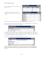
The target variable is Cost, and it should be minimized. The change variables are Oil, Rubber,
and Carbon, with lower bounds set as 0, 25, and 50. Upper bounds are set as 100, 60, and 100.
These bounds are based on the assumption that Weight is 100. Here are the constraints.
Weight = 100
TS => 12
E => 16
H => 25
H <= 35
The Optimizer (F11) returns the following solution.
This example model is located in the Optimization section of the TK Library, in the Optimizer
Examples group.
7-23
Part 2—Equation Solving
Portfolio Optimization: The Scenario Approach
Given a collection of scenarios and the probabilities associated with them, we can determine the
configuration resulting in the optimal outcome. This approach can be used in a variety of situations,
including investment portfolio management.
This TK table summarizes seven scenarios for
a portfolio of three investments. The values
are the expected decimal fraction returns over
the next 12 months. For example, scenario 3
predicts that the second investment will return
32.1% over the next year.
The probabilities associated with each of these scenarios are
contained in the following list.
The expected return from each of these scenarios can be computed if we input the fraction we invest
in each of the three equities. We can expand our input table to include these fractions.
7-24
Chapter 7—Solution Optimizer
For each of the scenarios, the expected return is computed as the “dot product” of the returns list and
the list of the fraction invested. In TK terms, this is represented as r = DOT('s1,'F). Since we
need to do this for each of the seven scenarios, we can use a procedure function. We create the
function and call it port. Here are the required statements.
These statements assume that a TK matrix, s, has been created. The list s is simply a list of list names.
Now we can call the port function from the Rule Sheet.
The resulting list of r values can be included in a
table with the corresponding probabilities. These are
the probabilities and returns associated with each of
the seven scenarios. Note that the sum of the
probabilities is 1.
7-25
Part 2—Equation Solving
It is now possible to compute the overall expected return, multiplying the expected returns by the
associated probabilities, and summing the results. This is another job for the DOT function. The
required statement is added to the port procedure function.
E = dot('r,'P)
The variance of the returns is then
computed using another loop within the
procedure. For each scenario, the overall
expected return is subtracted from each
of the expected scenario returns. That
difference is squared and the result
multiplied by the associated probability.
The results are then summed. The
required statements are added to the
port procedure function. Here is the
complete function.
The local variables E and v are declared as Output Variables in the function and the rule is modified
to accept the change.
Solving (F9), the Variable Sheet displays the results for the collection of inputs in the tables.
A common goal in investing is to obtain a certain expected level of return with a minimum variance.
In other words, there may be many ways of obtaining a particular level of return but those that are
more likely to result in greater fluctuations from the expectation are sometimes less desirable. In this
case, we are interested in determining the fraction to invest in each of the equities, such that the return
is at least 15%, with minimum variance.
7-26
Chapter 7—Solution Optimizer
The target value for this problem is the variance, v. The change values are the three fractions in the
list F. The Optimizer requires that the change values be declared as variables so additional rules are
required. The PLACE function is used to place values from the Variable Sheet into list elements.
It is important to note the sequence of the rules. The port function assumes that the values have
already been placed into the F list, so the function call should follow the rules that perform that task.
The Variable Sheet is updated as shown below.
The Optimizer can now be set up to solve the problem.
7-27
Part 2—Equation Solving
Constraints are added. We assume that the fractions must total 1 and that the minimum return is 15%.
Bounds are also placed on the three change variables, forcing them to be equal to or greater than zero.
That is, short selling is not considered.
After a few iterations, the solution is displayed on the Variable Sheet. You might investigate what
happens as the minimum expected return is changed, as well as what happens if the bounds are
removed.
7-28
Chapter 7—Solution Optimizer
Differential Equations and the Optimizer
This is a very rigorous exercising of many different TK Solver features, starting with the solution of
differential equations and concluding with use of the Optimizer to backsolve the problem.
Suppose one needs to solve the following differential equations for x = 0.1, 0.2, … 1.6,
with initial conditions y(0.1) = 0.2 and z(0.1) = 1.0:
TK Solver includes several built-in functions for solving differential equations numerically. They are
all used similarly. For this example, the ODE_RK4 function is used.
The ODE_RK4 function requires three inputs. The first represents the differential equations. If there
are simultaneous differential equations, a TK procedure function must be used to define the set. For this
example, a function called test2 is used to hold the equations. The second input to ODE_RK4 is the
reference to the list containing the values of the independent variable. These are the values at which the
differential equations are to be integrated. The list x is used here. The last input to ODE_RK4 is the
name of the list containing the solution list names. In this case, we will have two solution lists because
we have two differential equations. The list Y will be used to store the two solution list names.
The next step is to create the list Y on the List Sheet and fill it with the solution list names. The names
y and z are used for the two solution lists.
Here are the contents of the list Y.
A table can be used to store the independent variable and solution values.
7-29
Part 2—Equation Solving
Here are the definitions of the content lists for the
table Solution.
The table is used to supply the values of the
independent variable and the initial conditions for
y and z.
The List Fill Command is used to fill the x list with values from 0.1 to 1.6 in steps of 0.1.
The next step is to create the TK procedure function test2, which defines the set of simultaneous
differential equations. Here are the statements required.
The variable x is the independent variable. The variable y` represents the derivative with respect to
the independent variable x. The variable y represents the function with respect to x. The expression
y`[i] represents the derivative of the ith function with respect to x. Likewise, the expression y[i]
represents the value of the ith function at the value of x.
The variables are mapped to the calling ODE_RK4 function as follows.
The input variables must be defined in the proper sequence in order for the built-in ODE_RK4
function to work properly. The sequence must represent the derivative, function, and independent
variable values respectively. Because these are passed into the function they are declared as Input
Variables.
7-30
Chapter 7—Solution Optimizer
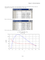
The program is now ready to solve the problem. Click the solve icon and the solution values are
displayed in the table. Here are the first 6 elements of the table.
Here are the last few elements.
We can easily create a TK Line Chart to plot y and z vs. x.
7-31
Part 2—Equation Solving
If these solutions are to be used in other parts of the model, they can be applied in TK List Functions.
Here is the definition of the y function.
The x list is used as the domain of the
function. The y list is used as the range
list. Using linear interpolation, the
function will be continuous over the
entire domain of x. The function will be
undefined for values of x outside the
domain.
Here are a few elements of the values used in the function.
The fz function is set up in the same way. We can now reference these functions anywhere else in the
model. Here are two rules on the rule sheet.
If we enter a value of 0.2135 for x on the Variable Sheet, we can solve for y and z.
We can also input a value for y and solve for x.
7-32
Chapter 7—Solution Optimizer
It is important to note that TK List Functions backsolve directly and always return the first solution
they find. In this case, there are two solutions as can be seen from the solution plot. It looks like there
should be another solution somewhere near x = 0.95.
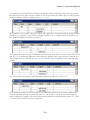
TK Optimizer can be used to find this solution. The Optimizer is configured with the Target Variable
defined as y, set equal to 1, and with the Change Variable set as x. Using bounds of 0.8 and 1 for x,
the Optimizer displays the following solution.
The Optimizer can also be used to determine an intersection point for the y and z curves. We enter a
rule, d=y-z, to define the difference between the two functions. We set the objective function as d
with a target value of 0. Bounds are set on x of 0.1 and 0.3 and the Optimizer returns the following
solution.
The second intersection point can be found by setting the bounds on x of 1.4 to 1.6.
The Optimizer can also be used to backsolve the differential equations for an initial condition that
results in a desired solution at a particular value of x. To do that, a rule is created which maps the
initial conditions to variables. The PLACE function performs this task, placing the values of yi and
zi into the first elements of the associated lists.
7-33
Part 2—Equation Solving
These rules must be inserted above the ODE_RK4 function call. Otherwise, they will not be applied
until after the integration has been completed using the prior values.
The initial conditions are input on the Variable Sheet.
Try changing zi from 1 to 1.2. The effect can be seen on the plot. The z function is raised.
The Optimizer can be used to determine the value of zi which forces the y and z curves to intersect
at x = 1. The target variable is set as d with a target value of 0 again. This time, zi is used as the
decision variable, with bounds of 1 and 1.5. Here is the solution.
7-34
Chapter 7—Solution Optimizer
The plot confirms the solution.
7-35
Part 2—Equation Solving
Repeated Optimization, Subject to Constraints
This example is taken from Engineering Optimization, Methods and Applications by G.V. Reklaitis, A.
Ravindran, and K. M. Ragsdell (John Wiley & Sons, 1983).
A natural gas pipeline transmission system is required to pump 100x1012 cu. ft./day (100
MMSCF/day) of natural gas over a distance of 600 miles. Compressor stations are to be placed at
equal distances. The design variables are the pipe diameter zD, the compressor discharge pressure P1,
and the distance between stations, L. The optimum design should be such that the total annual cost of
amortization and running of the pipeline, T, is minimized. If this minimum cost depends on the flow,
it should be evaluated for a given set of values.
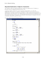
We create a TK model with the following equations:
7-36
Chapter 7—Solution Optimizer
After testing the model let us seek the ideal input values for a flow of 1,405,790 SCF/hr, proceeding
as in the previous examples.
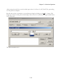
But this time we have constraints: to record them we begin by clicking on the Add… button. This
brings up a form for setting those relationships. Enter a series of constraints by using the Add button
in the form itself:
The final constraints set is:
7-37
Part 2—Equation Solving
Optimizing, we find the best parameters for that flow volume:
7-38
Chapter 7—Solution Optimizer
In order to store the optimum inputs for flows within a range:
1)
2)
3)
4)
5)
We associate lists2 with the relevant variables, Q, L, D, P1 and T.
For handling ease, we collect these lists into a table.
We run the Optimizer with the current set of values.
We save the results in the relevant lists by using Command  Put Values to Lists…
We repeatedly do the same with the other sets of values.
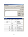
After repeating the process for all values of Q we have the following table of results:
It is frequently more informative to present list results in plot form:
2
Notice that we are NOT going to List Solve (F10)
7-39
Part 2—Equation Solving
(using log/log scales)
(or log-linear scales)
7-40