Download Calibration for a Robotic Arm, using Visual Information

Calibration for a Robotic Arm,
using Visual Information
SYLVAIN
RODHAIN
Master of Science Thesis
Stockholm, Sweden 2008
Calibration for a Robotic Arm,
using Visual Information
SYLVAIN
RODHAIN
Master’s Thesis in Computer Science (30 ECTS credits)
at the School of Computer Science and Engineering
Royal Institute of Technology year 2008
Supervisor at CSC was Kai Hübner
Examiner was Danica Kragic
TRITA-CSC-E 2008:035
ISRN-KTH/CSC/E--08/035--SE
ISSN-1653-5715
Royal Institute of Technology
School of Computer Science and Communication
KTH CSC
SE-100 44 Stockholm, Sweden
URL: www.csc.kth.se
Abstract
In order to use a static sensor (such as a camera) for robotic grasping
applications, the position and orientation of the sensor with respect to the
robot manipulator must be known. Finding this position is equivalent to
nding the transformation matrix in space between the robot's frame and the
sensor's frame, here referred as calibration.
The transformation matrix T ∈ M4×4 can be obtained by moving the robot
arm and detecting its position in the camera's view. This leads to 3 equations
of the form BTi − Ai = 0, where A ∈ M4×n is a matrix containing the
successive coordinates of the robot in space, B ∈ M4×n those of the camera
and Ai and Ti being the coordinates of A and T respectively, in only one
dimension (X , Y or Z ). This is solved using the Moore-Penrose pseudo inverse,
thus minimizing the mean square error.
The process is implemented in a network architecture, and a specic equipment is used. Tests are performed to estimate the precision of such a calibration and approximate the amount of motions required. Finally, the calibration
will allow other users to create systems using the robot manipulator to perform grasps or further manipulation of objects. It will also be required when
trying to perform smooth motions and imitations of human behavior.
Contents
1 Introduction
1.1 Background . . . . . . . . . . .
1.1.1 Classication . . . . . .
1.1.2 Purpose of the Thesis . .
1.2 Description of the Project . . .
1.2.1 Objectives of the Thesis
1.2.2 Requirements . . . . . .
1.3 Outline . . . . . . . . . . . . . .
.
.
.
.
.
.
.
.
.
.
.
.
.
.
.
.
.
.
.
.
.
.
.
.
.
.
.
.
.
.
.
.
.
.
.
.
.
.
.
.
.
.
.
.
.
.
.
.
.
.
.
.
.
.
.
.
.
.
.
.
.
.
.
.
.
.
.
.
.
.
.
.
.
.
.
.
.
.
.
.
.
.
.
.
2 Theoretical Background
2.1
2.2
2.3
2.4
2.5
Visual Servoing . . . . . . . . . . . . . . . . . . . . .
Calibration for Eye in Hand . . . . . . . . . . . . . .
Calibration for Eye to Hand . . . . . . . . . . . . . .
Pose Estimation Algorithm . . . . . . . . . . . . . . .
Least Square Error Algorithm . . . . . . . . . . . . .
2.5.1 Reconstruction in 3D from Visual Information
2.5.2 Finding the Transformation Matrix . . . . . .
2.5.3 The Moore-Penrose Pseudo Inverse . . . . . .
2.5.4 Conclusion . . . . . . . . . . . . . . . . . . . .
3 Implementation
3.1 System Setup . . . . . . . . . . . . . .
3.1.1 Kuka Arm - Robot . . . . . . .
3.1.2 Videre STOC Device - Cameras
3.2 Communication Process . . . . . . . .
3.2.1 NOMAN Architecture . . . . .
3.2.2 System's Architecture . . . . .
3.3 Robot's Client . . . . . . . . . . . . . .
3.3.1 KUKA's Script and Language .
3.3.2 General Presentation . . . . . .
3.3.3 tinyXML Parser . . . . . . . . .
3.3.4 Problems . . . . . . . . . . . .
3.4 Cameras' Client . . . . . . . . . . . . .
3.4.1 Frame Grabber . . . . . . . . .
3.4.2 General Presentation . . . . . .
3.4.3 Arm Position Detection . . . .
3.4.4 Filter Applied . . . . . . . . . .
3.4.5 Problems . . . . . . . . . . . .
3.5 Summary . . . . . . . . . . . . . . . .
.
.
.
.
.
.
.
.
.
.
.
.
.
.
.
.
.
.
.
.
.
.
.
.
.
.
.
.
.
.
.
.
.
.
.
.
.
.
.
.
.
.
.
.
.
.
.
.
.
.
.
.
.
.
.
.
.
.
.
.
.
.
.
.
.
.
.
.
.
.
.
.
.
.
.
.
.
.
.
.
.
.
.
.
.
.
.
.
.
.
.
.
.
.
.
.
.
.
.
.
.
.
.
.
.
.
.
.
.
.
.
.
.
.
.
.
.
.
.
.
.
.
.
.
.
.
.
.
.
.
.
.
.
.
.
.
.
.
.
.
.
.
.
.
.
.
.
.
.
.
.
.
.
.
.
.
.
.
.
.
.
.
.
.
.
.
.
.
.
.
.
.
.
.
.
.
.
.
.
.
.
.
.
.
.
.
.
.
.
.
.
.
.
.
.
.
.
.
.
.
.
.
.
.
.
.
.
.
.
.
.
.
.
.
.
.
.
.
.
.
.
.
.
.
.
.
.
.
.
.
.
.
.
.
.
.
.
.
.
.
.
.
.
.
.
.
.
.
.
.
.
.
.
.
.
.
.
.
.
.
.
.
.
.
.
.
.
.
.
.
.
.
.
.
.
.
.
.
.
.
.
.
.
.
.
.
.
.
.
.
.
.
.
.
.
.
.
.
.
.
.
.
.
.
.
.
.
.
.
.
.
.
.
.
.
.
.
.
.
.
.
.
.
.
.
.
.
.
.
.
.
.
.
.
.
.
.
.
.
.
.
.
.
.
.
.
.
.
.
.
.
.
.
.
.
.
.
.
.
.
.
.
.
.
.
.
.
.
.
.
.
.
.
.
.
.
.
.
.
.
.
.
.
.
.
.
.
.
.
.
.
.
.
.
.
.
.
.
.
.
.
.
.
.
.
.
.
.
.
.
.
.
.
.
.
.
.
.
.
.
.
.
.
.
.
.
.
.
.
.
.
.
.
.
.
.
.
.
.
.
.
.
.
.
.
.
.
.
.
.
1
1
1
2
2
2
3
4
5
5
6
7
8
9
10
11
13
15
17
17
17
18
19
19
20
24
24
24
24
26
26
26
27
27
32
33
33
4 Evaluation
35
5 Conclusion
51
6 Bibliography
53
A Cameras' Frame Grabber Parameters
55
B Board Layout of the Electronic Circuit
60
C Cameras' CCD Array Response
61
D KUKA Workspace Protection
62
E Noman Conguration File
64
4.1 Filter Parameters . . . . . . . . . . . . . . . . . . . . . . . . . . . . . 35
4.2 Position Errors . . . . . . . . . . . . . . . . . . . . . . . . . . . . . . 43
List of Figures
1
2
3
4
5
6
7
8
9
10
11
12
13
14
15
16
17
18
19
20
21
22
23
A Barrett Hand, a robotic hand equipped with 3 ngers. The opposable thumb (numbered as F 3 on he picture) can not be rotated
around the palm, while the two other ngers have the same opening
angle. . . . . . . . . . . . . . . . . . . . . . . . . . . . . . . . . . .
ARMAR-III, a humanoid platform [2] . . . . . . . . . . . . . . . . .
Eye in Hand calibration problem: how to nd the X matrix ? . . .
User Cases Diagram showing the requirements for performing a calibration . . . . . . . . . . . . . . . . . . . . . . . . . . . . . . . . . .
An iteration of POSIT algorithm . . . . . . . . . . . . . . . . . . .
The Eye in Hand calibration problem in our system: how to nd the
T matrix? . . . . . . . . . . . . . . . . . . . . . . . . . . . . . . . .
KUKA Robot arm installation . . . . . . . . . . . . . . . . . . . . .
STH device, by Videre Design, used for the preliminary tests [12] .
STOC device, by Videre Design, used for the experiments [13] . . .
NOMAN Communication package Class Diagram . . . . . . . . . .
Specic Implementation Class Diagram . . . . . . . . . . . . . . . .
TestServerCalibration State Diagram. A small description of the
UML norm can be found in section 3.2.2. . . . . . . . . . . . . . . .
TestClientRobot State Diagram. A small description of the UML
norm can be found in section 3.2.2. . . . . . . . . . . . . . . . . . .
TestClientCameras State Diagram. A small description of the UML
norm can be found in section 3.2.2. . . . . . . . . . . . . . . . . . .
Electronic schema . . . . . . . . . . . . . . . . . . . . . . . . . . . .
Voltages . . . . . . . . . . . . . . . . . . . . . . . . . . . . . . . . .
Metallic box with blinking diode . . . . . . . . . . . . . . . . . . . .
Left view of the cameras . . . . . . . . . . . . . . . . . . . . . . . .
Two successive images from the left camera. Although it might not
be visible, in the left picture, the diode is o and it is lit up in the
right one. . . . . . . . . . . . . . . . . . . . . . . . . . . . . . . . .
Histogram of pixels' luminosity dierence, a pixel's intensity ranges
between 0 and 255. . . . . . . . . . . . . . . . . . . . . . . . . . . .
Luminosity dierence between two images, thresholded at T units per
pixel, with T ∈ {4, 10, 20, 30, 50, 70}. . . . . . . . . . . . . . . . . .
Sum for 20 images of the luminosity dierence thresholded at T = 20:
the result is scaled so that a pixel with a value of 20 (maximal value)
is represented in black. . . . . . . . . . . . . . . . . . . . . . . . . .
Histogram of resulting pixels' values after summing up the dierence
of luminosity in 20 images, thresholded at T = 20. . . . . . . . . . .
.
.
.
2
3
6
.
.
7
8
.
.
.
.
.
.
11
17
18
18
19
21
. 23
. 25
.
.
.
.
.
28
29
30
32
35
. 36
. 36
. 36
. 37
. 38
24
25
26
27
28
29
30
31
32
33
34
35
36
37
38
39
40
41
Results of summed up luminosity dierence, with a threshold at T
units per pixel, with T ∈ {1, 2, 5, 10, 15, 18}. . . . . . . . . . . . . . .
Result, when ltering the sum for 20 images of the luminosity dierence thresholded at T = 20: the result is scaled so that a pixel with
a value of 180 (maximal value) is represented in black. . . . . . . . .
Histogram of pixels' value, post ltering . . . . . . . . . . . . . . . .
Results ltered sum of luminosity dierence, with a threshold at T
units per pixel, with T ∈ {5, 10, 20, 50, 100, 150}. . . . . . . . . . . . .
Final estimation for the position of the diode . . . . . . . . . . . . . .
Histogram of the diode position in Y (top) and X (bottom) . . . . . .
Examples of small motions in the backgrounds, the left image shows
the view of the camera and the right image is the dierence of luminosity between this image and the next one. . . . . . . . . . . . . . .
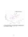
Reconstructed setup in 3D, showing cameras' and robot's frames origins, as well as the 3D box inside of which the points will be taken
for calibration. . . . . . . . . . . . . . . . . . . . . . . . . . . . . . .
3D representation of the calibration points and their error, for density
comparison (successively 8, 27 and 125 points), according to the axis
of projection (in the robot's frame). . . . . . . . . . . . . . . . . . . .
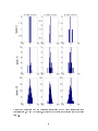
Histograms of the displacement's error on the three calibration sets
(successively 8, 27 and 125 points), according to the axis of projection
(in the robot's frame). . . . . . . . . . . . . . . . . . . . . . . . . . .
Histograms of the displacement's error on the test set (containing
200 points), using the three dierent calibration matrices (successively computed with 8, 27 and 125 points), according to the axis of
projection (in the robot's frame). . . . . . . . . . . . . . . . . . . . .
Representation in 3D of the test points in the robot's frame and the
cameras' frame, with the displacement error, according to the calibration computed with the large set of 125 points. . . . . . . . . . . .
Original, not rectied picture, extracted from the STOC device . . .
Comparison of rectication on chip (left picture) and rectication on
computer (right picture) for a picture extracted from the STOC device
Comparisons of color algorithms, Fast (left picture) and Best (right
picture) . . . . . . . . . . . . . . . . . . . . . . . . . . . . . . . . . .
Strip board layout . . . . . . . . . . . . . . . . . . . . . . . . . . . .
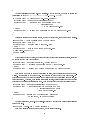
Imager Response - Color . . . . . . . . . . . . . . . . . . . . . . . . .
Filter Transmittance . . . . . . . . . . . . . . . . . . . . . . . . . . .
38
39
40
40
41
41
42
43
44
46
47
48
55
56
56
60
61
61
1 Introduction
As technologies improve and as the standards of living increase, the eld of home
automation keeps on extending. The next generation of robots will be operating in
private environments and therefore, they need to be very adaptive. Cameras are, for
that matter, perfect sensors as they provide a wide range of possible information.
A problem arises when trying to manipulate objects. Without talking about
the diculties laying in the grasp of an object, as long as the visual information
is not related to the environment of the robot, it is not able to interact properly
with its surroundings. Have you never felt surprised when growing up, going back
to old places and seeing how doors were smaller? Or how a light switch in a room
was located at a dierent height? Those are relations of the human body to its
environment. There is a similar relation of the vision system to the hands.
While humans learn those inner relations at a young age and keep on improving
at every motion, the robot can dene specically those relations between its vision
system, the environment and its hands. The process of calibration as described
further in this paper consists of dening the relation between the vision system and
the hands of the robot. The aim is that, in the end, the robot knows how to reach
for objects in its eld of vision.
Notice that humans do not dene this relation between their vision system and
their hands too precisely. The proof being that when looking at an object and
keeping your eyes closed afterwards, it is hard to grasp the object in a precise way.
Humans have an estimation of the relation between their body and their eld of
vision but, when performing actions, they also permanently adjust the position of
their hands.
1.1
Background
1.1.1 Classication
This project was carried out at CVAP/CAS (Computer Vision & Active Perception / Center for Autonomous Systems), a department of KTH. Generally, the work
is included in the PACO PLUS research. PACO PLUS [1] is a European project
aiming at designing robots which are able to learn about their surroundings and
to interact with their environment. PACO PLUS main aspect is that objects are
intimately related to the actions that can be performed with them. The grasping
attributes of an object and grasping capacities of a robot are therefore a main part
of the research at CVAP.
1
1.1.2 Purpose of the Thesis
The nal purpose of the calibration process is to mount a mechanic hand (see Figure 1) on a robot arm and to make reality tests for grasping. Up to now, most of
the experiments were being conducted on a 3D simulator, GraspIt!1 .
Figure 1: A Barrett Hand, a robotic hand equipped with 3 ngers. The opposable
thumb (numbered as F 3 on he picture) can not be rotated around the palm, while
the two other ngers have the same opening angle.
Additionally, there has been a complete humanoid platform built at the Karlsruhe University (Germany) a partner of PACO-PLUS [2]. This platform can be
seen in Figure 2. The department of CVAP is working in parallel, using a replica
of the humanoid head. Once the robot arm is calibrated relatively to the head, a
complete system can be tested to perform recognition of objects, focusing of the
cameras, estimation of grasping points and grasping attempts, for example.
1.2
Description of the Project
1.2.1 Objectives of the Thesis
The system must provide an estimation of the position and the orientation of the
arm (the robot's frame) relatively to the cameras' frame so that vision can be used
to detect a point in the workspace, estimate its 3D coordinates and bring the robot
manipulator at this precise location. The estimation of this transformation in space
is a phase usually done by hand. It is an annoying and time-consuming task which
needs to be repeated every time the robot arm or the cameras are moved (the relation
in space would then be modied).
1 GraspIt!
is a software developed in the Computer Science department of Columbia University,
home page :http://www1.cs.columbia.edu/~allen/PAPERS/graspit.final.pdf [3].
2
Figure 2: ARMAR-III, a humanoid platform [2]
Finally, the project has to provide an easy mean of communication with a KUKA
arm2 as well as the possibility for any user to drive the robot to a specic position.
Technically, the estimation of this position will be computed from visual information, likely from a rigidly linked pair of cameras. Therefore the system should also
implement an algorithm for 3D reconstruction.
One should also consider, that despite lens correction for the cameras, the calibration (i.e. the transformation in space from one frame to another) is nonlinear
due to errors in the calculations and optimized for a determined working space. So
one might need to re-calibrate, even when using almost the same settings, simply in
case the objects are in a dierent area.
1.2.2 Requirements
The requirements for the system are very logic ones, when it comes to coding. The
system should be kept simple and easy to re-use. The system should be coded in
C++ as most of the work in CVAP/CAS is done; this ensures the system may
be modied by other people, later on. There is a library of C/C++ sources at the
CVAP/CAS department, called NOMAN. NOMAN contains a communication package, providing a stable base for the implementation of a multi-threaded client-server
architecture. Many other robots at the CVAP department have already been coded
verifying this architecture. Consequently it shall also be used for this project. One
advantage is that the system can be used on a single computer, or over the network.
This will give more freedom in the organization of sensors (as video treatments in
2 KUKA
Roboter GmbH is a company producing industrial robots, more details about the
specic arm used can be found in section 3.1. More general information about KUKA can be
found on their ocial website: http://www.kuka.com.
3
particular may require their own calculation unit).
Finally, as it will be explained in section 3.1, a specic equipment has been
provided for testing the calibration and a part of the work will be to apply the
calibration to this equipment. The system has to implement a frame grabber for a
pair of rigidly linked cameras: a STOC (Stereo On Chip Processing) device from
Videre3 , as well as to provide a control over the network of a robot arm: a KUKA
robot arm with 6 degrees of freedom.
1.3
Outline
Section 2: Theoretical Background presents the possibilities that have been
considered for the calibration algorithm and solutions used by other people if their
setup is dierent. It also describes two specic methods that were studied further
and presents some simple mathematical notions for dening the calibration of two
frames in space.
Section 3: Implementation is the main part of this report. It deals with all
the performed work, whether it is related to hardware or software. It explains the
provided equipment, the structure of the communication process as well as any
additional task which has been required.
Section 4: Evaluation presents results from the calibration, in terms of error
in space, depending on the number of points used for calibration and the image
ltering parameters.
Section 5: Conclusion describes future potential work and brings the report to
an end.
3 Videre
Design is a company producing vision hardware and software, as well as mobile robots.
More information can be found on their website: http://www.videredesign.com/. For specic
information about the vision device used for the project, see section 3.1.2.
4
2 Theoretical Background
As it was shortly presented in the introduction, human behavior is based upon real
time control, rather than a permanent relation between vision and their hands. As
we are trying to imitate human behavior, the research was rst oriented towards a
close loop control of the robot manipulator at a frame rate, called visual servoing.
Also, when conceiving a robot equipped with manipulators meant to work in a
human environment, one may wonder whether the sensors should be attached to
the static structure of the robot or on its manipulator. For non-mobile applications
or embedded systems with little degrees of freedom, the idea to mount a sensor on
the manipulator is to increase its liberties and the range of accessible points. But
when the platform is highly evolved, there is no need to add degrees of freedom to
the sensors.
Apart from deciding upon the type of equipment, one may also consider the
type of application, as for example, reconstruction of objects in three dimensions
would be easier to provide with a camera mounted on a robot arm, turning around
the object without touching it. While if using static cameras, the same application
would require the arm to grasp and show around an object to cameras.
A humanoid robot has to provide a wide range of possible positions and orientations for the vision system, so that, just like humans do, the robot could look at a
scene the way it requires. It also needs to be adaptive to any application a human
might do or require it to perform. It is logic to keep the structure similar to a human
body and it would be unnecessary and inecient to put the visual sensors only on
a manipulator.
However, the eld of research with sensors mounted on the manipulator (this
setup is called "Eye in Hand" opposed to a setup where cameras stand alone, called
"Eye to Hand") has to solve the same calibration problem, i.e. has to nd the static
relation between the wrist of the robot and the sensor directly attached to it.
2.1
Visual Servoing
The principle of visual servoing consists of extracting features from images and
producing a control command at a video frame rate. Those techniques were only
available since there happened to be heavy improvements in calculation power during
the last decade, image treatment being generally an expensive process.
When using a stereo rig for visual input, two main types exist, whether the output
of the control loop is steered by either features in 2D, extracted from both views, or
features extracted from a 3D reconstruction of the working area. A nice tutorial on
visual servoing can be found in [4]. Hybrid techniques were also developed, providing
new possibilities and solving some stability issues such as 2.5D Visual Servoing [5].
Visual Servoing is mostly researched with "Eye in Hand" setups, but it can even
5
be applied when using "Eye to hand" setups, by extracting features from both the
scene and also from a robot arm. This possibility, described in [6], was of strong
interest for our system, that we wanted similar to human behavior. Although some
techniques of visual servoing only require a low quality calibration, or may provide
their own, there is still a need to dene, even roughly, the relation in space between
the cameras, and the robot's frame or the robot's wrist. In the next section, we will
approach a method applied to calibrate an "Eye in Hand" setup.
2.2
Calibration for Eye in Hand
When looking for calibration of a setup with the sensor attached to the wrist, this
technique is one of the most ecient and simple ones. It is meant to be used when
a single or a pair of rigidly linked cameras is mounted on a robot manipulator. The
unknown relation X is the one between the robot wrist's frame H to the sensor's
frame E , the sensor being, as can be seen in Figure 3, a camera.
Figure 3: Eye in Hand calibration problem: how to nd the X matrix ?
Image extracted from the website :
http://wwwnavab.in.tum.de/Chair/HandEyeCalibration
The principle, described in [7] and [8], is to drive the manipulator4 to some
known positions in space, while aiming the camera at a specic static object whose
3D structure and metric are known. In such cases, for each position, the camera
can estimate its position relatively to the object. By repeating this process, one
can estimate the space transformation between the manipulator frame and the camera's frame. In most cases, to improve calibration accuracy, many views will be
used. The time required for extracting the image features and computing the space
4 The
stereo cameras, represented in Figure 3, at the T frame can be replaced by a well internally
calibrated robot, with its manipulator attached at the H frame. Therefore Ai and Aj result from
odometry, see Figure 6.
6
transformation is negligible compared to the time required for moving the robot
manipulator.
2.3
Calibration for Eye to Hand
Inspiring ourselves from the previous systems used for controlling a hand, we decided
what was required for our own system. Unfortunately the controller system provided
with the KUKA arm did not allow us to do real time control. It only permitted
motions step by step, with no interferences, neither when interpolating a motion,
nor conducting the robot arm to a location in space. As we discovered visual servoing was not physically available, we focused on doing a highly precise calibration
consequently further from the abilities of a real human considering grasping. Such
a calibration required three main elements to be done, as already described earlier
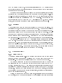
in the introduction (in section 1.2.1), those elements are organized in Figure 4.
Figure 4: User Cases Diagram showing the requirements for performing a calibration
The system must be able to relate positions in space in both the robot's frame
and the cameras' frame. To perform this, the system has to be able to drive the robot
to dierent locations and also needs to extract some visual information (either in
2D or 3D). Finally, It must provide an algorithm for computing the transformation
matrix in space. The choice of this algorithm was not specied. Two dierent
attempts were made successively, those attempts are presented in the two sections
coming next.
7
2.4
Pose Estimation Algorithm
A diculty arises when using a single static camera. When calibrating the robot
relatively to such a single camera, the user has no access to depth estimation or
any disparity map5 accessible when using stereo cameras. The algorithm POSIT
described in [9] gives a standard way to deal with such cases, when the 3D structure
and dimensions of the observed object are known.
Figure 5: An iteration of POSIT algorithm
It consists of estimating the rotation matrix rst and then the translation between the camera's frame and the robot's frame. The estimation of the transformation matrix is performed in an iterative way. Using a rough estimation of the
transformation matrix, it produces a scaled orthographic projection of the known
3D structure (the points where the robot has been driving). Then it approximates
5A
disparity map is an image representing the estimated depth of each pixel. It can be visualized
in a grayscale picture with dark pixels representing the background points and bright pixels showing
short distances. A disparity map is strictly equivalent to calculating the 3D reconstruction for the
complete set of pixels, but it has nicer visualization properties.
8
the points in the image to their equivalent in the scale orthographic projection and
improves if required the estimated value of the axis of the robot's frame (i.e. the
estimated value of the rotation matrix).
In Figure 5, you can see how the iteration is performed. G is the image plane, K
is the plane on which the scaled orthographic projection of the object is performed.
This plane is computed from the previous estimation of the depth of one point (here
the depth estimation of M0 , which is Z0 given as an initial value).
For the rst iteration, the robot's frame is completely unknown. In the image
plane, the point M0 appears as m0 , and any other point Mi as mi , however, as the
depth of Mi is unknown, it is considered to be equal to Z0 , until the robot's frame
is approximated. Therefore, the point Pi is considered to be the one whose image
is mi . This will allow to perform a rough estimation from the image of the couple
of vectors (i, j) (dening the camera's frame basis), by the rotation matrix, in the
robot's frame axis, even if the image (u, v) of the couple (i, j) is not orthogonal.
By using the cross product, one can estimate the depth axis (i.e. w in the robot's
frame, the image of k). This gives an estimation of the rotation matrix as the
rotation matrix can be written as the set of columns containing (u, v, w), the images
of (i, j, k).
At the next iteration, the scaled orthographic projection (estimation of Mi as
Pi ) will be slightly improved, due to a better knowledge of the depth of every point,
and Pi will be closer from Ni which would be the perfect perspective projection of
Mi if the transformation matrix was known.
At rst, we were using a set of two cameras loosely attached. The external calibration (position and orientation from one camera to the other), if not properly
performed, could be a risk of a loss in precision for the calibration of the arm relatively to the cameras. The POSIT algorithm was tested but nally not implemented,
since, later on, the visual input was carried out by a rigidly linked pair of cameras
with an internal calibration done at the factory (more information on the cameras
can be found in the section 3.1.2)6 .
2.5
Least Square Error Algorithm
As the previous algorithm was showing risks of inaccuracy, we also tested another
algorithm, exploiting further possibilities of the cameras. This algorithm is working
with 3D points, preventing the lack of knowledge on the depth of points.
6 Indeed,
the single reason for using this algorithm was to avoid the requirement of a precise
external calibration. In the preliminary test phase, the results obtained with POSIT (i.e. two
independent calibrations on single cameras) were similar to those obtained later when doing a
single calibration on a pair of rigidly linked cameras, already externally calibrated.
9
2.5.1 Reconstruction in 3D from Visual Information
The internal calibration of a camera is a matrix M ∈ M3×4 . This matrix is equal
to the product of rectication matrix of the camera K ∈ M3×3 by the projection
matrix P ∈ M3×4 . Let p = (x, y) ∈ R2 be the image of P = (X, Y, Z) ∈ R3 , in
the camera characterized by M . When writing the coordinates homogeneously, we
have:
 
 




X
X
x/λ
m11 m12 m13 m14
Y 
Y 


  
  
y/λ = M ∗   = m21 m22 m23 m24  ∗   .
Z 
Z 
λ
m31 m32 m33 m34
1
1
Therefore, for every point P in 3D, we get two equations :
m11 X
m31 X
m21 X
y=
m31 X
x=
+ m12 Y
+ m32 Y
+ m22 Y
+ m32 Y
+ m13 Z + m14
+ m33 Z + m34
+ m23 Z + m24
+ m33 Z + m34
which can be written as :
(xm31 − m11 )X + (xm32 − m12 )Y + (xm33 − m13 )Z + (xm34 − m14 ) = 0
(ym31 − m21 )X + (ym32 − m22 )Y + (ym33 − m24 )Z + (ym34 − m24 ) = 0
When using a pair of cameras a and b externally calibrated (that is we know the
relation in space between both cameras), and when knowing the internal calibration
matrix from one camera, say Ma , we can nd the internal calibration matrix from
the second camera, Mb . This gives us a set of four equations similar to the two
previous ones. The complete set can be written in a matrix form:

(xa ma31 − ma11 ) (xa ma32 − ma12 ) (xa ma33 − ma13 ) (xa ma34 − ma14 )




  


X
(y a ma − ma ) (y a ma − ma ) (y a ma − ma ) (y a ma − ma )
31
21
32
22
33
24
34
24   


 Y 

∗ =0
 Z 
 b b
 (x m31 − mb11 ) (xb mb32 − mb12 ) (xb mb33 − mb13 ) (xb mb34 − mb14 ) 


1




(y b mb31 − mb21 ) (y b mb32 − mb22 ) (y b mb33 − mb24 ) (y b mb34 − mb24 )
And we can solve the three unknown coordinates (X, Y, Z) of the 3D point P, by
solving this linear set of four equations.
10
2.5.2 Finding the Transformation Matrix
The new vision equipment was provided with a complete, highly precise internal and
external calibration, reducing the interest that could lay in the use of the POSIT
algorithm to nothing. The principle for such a calibration using the least-squares
error algorithm is strongly inspired by the calibration for an "Eye in Hand" setup
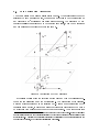
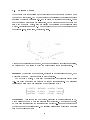
presented in section 2.2, and is represented in Figure 6.
Figure 6: The Eye in Hand calibration problem in our system: how to nd the T
matrix?
By driving the robot to dierent positions and storing the 3D reconstruction of
the robot manipulator in the cameras' frame in memory, the user can obtain a set
of points, with their coordinates in both the robot's and the cameras' frame.
−
→ −
→
−
→ −
→ −
→
Let (−
x→
R , yR , zR ) and (xC , yC , zC ) be the Euclidean basis for the robot's frame, of
origin OR , and the camera's frame, of origin OC , respectively.
The rotation matrix R is dened as:

−
→ −
→



 R × xC = xR
−
→
R ∈ M3×3 , and :
R×−
y→
C = yR



−
→
 R×−
z→
C = zR
The translation vector t is dened as:
 
tx
 
t ∈ M3×1 ,t = ty  and OC + t = OR
tz
11
Therefore, when using homogenous coordinates, if a point PR in the robot's frame
is equivalent to a point PC in the camera's frame, with:
 
 
XR
XC
Y 
Y 
 R
 C
(PR , PC ) ∈ M4×1 2 , PR =   and PC =   ,
 ZR 
 ZC 
1
1
we can dene T the transformation matrix so that T × PC = PR by:

  
tx




 R  ty 



T =

t
z 

1
0 0 0
We have seen how to compute the 3D coordinates from points in the cameras'
frame. It seems that every couple of points (PCi , PRi ) would bring three equations,
and therefore, as there are 12 unknowns (9 for the rotation matrix and 3 for the
translation vector) we would need four points. However, considering a set of N
points, we can rewrite the equations with :
N
1 X
PCj
N j=1
0
PCi
= PCi − PC ,
with PC =
0
PRi
N
1 X
with PR =
PRj
N j=1
= PRi − PR ,
Consequently,
0
0
PRi
= PR + T × PCi


XCi − XC
Y −Y 
 Ci
C 
= PR + T × 

 ZCi − ZC 
0
Which means that the three unknowns (tx , ty , tz ) are not part of the equations,
and three points are sucient (of course, those three points need not be aligned,
otherwise some equations will be redundant).
When having more than three points, nding out the transformation matrix
between two frames is simply done by solving the over-determined system of linear equations, using the Moore-Penrose pseudo inverse.
As we can write out our system as:
















PR1  . . . PRN  = T ∗ PC1  . . . PCN 
12
which can be rewritten as:
(




 
 
XR1 . . . XRN = A ∗ TX  , YR1 . . . YRN = A ∗ TY  ,

h

with A = 

h
PC1
..
.
PCN
i
h
TX

)
 
ZR1 . . . ZRN = A ∗ TZ 
i
i
h



T

h Y i
, and T = 
,
i


TZ


0 0 0 1
then the system can be solved by using the Moore-Penrose Pseudo Inverse successively for the three lines of the transformation matrix.
2.5.3 The Moore-Penrose Pseudo Inverse
Disclaimer :
Having had diculties to nd a mathematical proof that the Pseudo Inverse is the
solution to the Least Square Error problem, I heavily inspired this section from a
handout provided by the Mechanical Engineering department of The California Institute of Technology. The original and complete version of the paper can be fetched
at http://robotics.caltech.edu/~jwb/courses/ME115/handouts/pseudo.pdf.
The Moore-Penrose pseudo-inverse is a general way to nd the solution of the
following system of linear equations:
→
−
−
b = A→
y
→
−
−
b ∈ Rm ; →
y ∈ Rn ; A ∈ Rm×n .
(1)
As we saw in the previous section, nding the transformation matrix in space
for calibration is equivalent to solving three equations of the type of (1), with:

→
−


b
=
J
.
.
.
J
R1
RN ,


→
−
y = TJ ,



A as dened previously,
with J ∈ {X, Y, Z}
Moore and Penrose showed that there is a general solution to these equations
→
−
−
(which we will term the Moore-Penrose solution) of the form →
y = A† b . The matrix
A† is the Moore-Penrose "pseudo-inverse".
13
When m > n, there are more constraining equations than there are free variables
→
−
in y . If we were working for simulated data, with a high resolution, only four
independent equations would be sucient, as any other point would provide an
equation which could be expressed as a linear combination of those four equations.
However, the data used is real and noise is present.
Hence, it is not generally possible to nd a solution to the set equations. The
−
−
pseudo-inverse gives the solution →
y such that A† →
y is "closest" (in a least-squared
→
−
sense) to the desired solution vector b . The Moore-Penrose pseudo-inverse provides
the solution which minimizes the quantity
→
−
−
k b − A→
y k.
To understand the Moore-Penrose solution in more detail, rst recall that the
ColSpace of A, denoted Col(A), is the linear span of its columns. If r is the rank of
matrix A, then it veries dim(Col(A)) = r. In the case where the points used for
calibration are not properly spread in space, we face the risk to have r < n. This
would mean that there is one dimension which is not "accessible" to the solution.
The transformation matrix would then be invalid.
→
−
→
−
But even if r = n, it is likely that b 6∈ Col(A) (if b ∈ Col(A) it means the data
→
−
set is free from any error). Therefore, we can project orthogonally b on Col(A),
→
−
and decompose b as a component in Col(A) and an orthogonal component:
→
−
−−→ −−−→
b = bCol + b⊥Col
→
−
There is one solution y 0 so that:
→
−
−−→
bCol = A† y 0
−−→
(2)
−−−→
Since bCol ∈ Col(A) and b⊥Col ∈⊥ Col(A) are orthogonal to each other, it must
be true by Pythagoras' theorem that:
→
−
−−→ −−−→
−−→
−−−→
k b k2 = kbCol + b⊥Col k2 = kbCol k2 + kb⊥Col k2 ,
→
−
and the Moore-Penrose solution y 0 is the one that minimizes the square distance to
→
−
b.
When A is full rank, the Moore-Penrose pseudo-inverse can be directly calculated
as follows:
A† = AT AAT
14
−1
2.5.4 Conclusion
We saw how to reconstruct points in 3D and by listing them, how to compute
the transformation matrix, using the Moore-Penrose Pseudo Inverse. However the
transformation matrix computed can be improved. This would be done by deleting
points that can be said absurd. Such points have their error to be too high. The
error is the distance between the position of this point in the cameras' frame once
translated into the robot's frame and its related position in the robot's frame.
The criteria for too high error is subjective. The smaller the error will have
to be, the better will be the Moore-Penrose solution to the set of linear equations.
However, this does not mean the solution will be optimal considering the whole set
of points, the solution being over-specic. On the other hand, if the threshold on
the error is too high, points that were badly estimated by the cameras will inuence
the solution, drifting away from the best transformation matrix. Those ideas were
taken into consideration while implementing the algorithm.
15
16
3 Implementation
3.1
System Setup
3.1.1 Kuka Arm - Robot
General information The arm used for the experiments is an industrial arm,
produced by KUKA Roboter GmbH. It is a robot arm with six joints, connected to
a robot controller (KRC). An external control panel (KCP) allows manual displacements and coding of scripts. The complete system is observable in Figure 7.
Figure 7: KUKA Robot arm installation
By using the client panel, the user can move the robot manually, observe the 3D
coordinates, dene new tools and new bases. This makes any testing step very easy,
as all the kinematic relations are handled internally. Besides, to prevent damaging
the environment through motion by the robot, or to restrict the workspace, the users
can dene protections in both Cartesian an axis-specic spaces. Those protections
can be either respected, or slightly violated (see section D for more information).
Controller's communication process The controller is handling all the com-
munication with the hardware. When using communication over the network, the
controller can only interpret XML messages. It is provided with a XML parser,
but has to be told before running what structure the messages will have. The controller can only execute scripts written in a specic language, described further in
section 3.3.1.
When setting a server, the user has to store the IP address and a server name
in a le called XmlApiCong.xml. Then the user has to create a le called serverName.xml, storing the XML structure, using a KUKA language for description of
XML tags and hierarchy. Further information can be found in the Ethernet KRL
documentation [15] of the KUKA robot.
17
3.1.2 Videre STOC Device - Cameras
Initially, the work started using two monocular cameras, mounted on a metallic
structure with a variable baseline, called STH (see Figure 8). The rst tests were
done with the STH device. This is why preliminary tests were started using the
POSIT algorithm described in section 2.4. Later on, we had to replace the device
but the new one was produced by the same company and the whole frame grabber
was working ne with the new cameras.
Figure 8: STH device, by Videre Design, used for the preliminary tests [12]
The cameras used for the experiments are a pair of rigidly linked cameras, also
produced by Videre Design (see Figure 9). The STOC device (STOC stands for
Stereo On Chip) is able to create disparity maps and estimate the 3D position of
any point in the image. Unfortunately, even if the overall disparity map is accurate,
there can be a lot of noise and the detection of a single pixel in both views is
relatively random, leading to absurd 3D positions. Hence, a specic detector was
designed for estimating the robot position and 3D reconstruction.
Figure 9: STOC device, by Videre Design, used for the experiments [13]
The cameras have an IEEE 1394 interface and a resolution of 640x480, with a
maximal frame rate of 30 fps (50 fps are reachable when reducing the frames size).
The baseline between both cameras is 90 mm and static. For the frame grabber,
more details can be found in the implementation, section 3.4.1, and in section A.
18
3.2
Communication Process
3.2.1 NOMAN Architecture
The NOMAN architecture, presented in the class diagram in Figure 10, describes
only the communication package included in NOMAN.
Figure 10: NOMAN Communication package Class Diagram
There is a very basic class (RecvBuInterface ), not represented in this class
diagram, which is encapsulating further methods for data handling over a socket
connection. MsgCommInterface derivates from this class and shows higher level
methods.
For sending a message, the client needs to prepare the head rst, calling the
prepareMsg method. This will take the type of message to send as an argument. The
type of message is typically helping dierent actors in the communication process
addressing the received data in the form of the correct structure.
The method waitForReply is an ecient way to await a message, whether this
message has to be of one specic or several types. The user can dene the waiting
time and the expected type of message, as well as the maximum time for waiting.
The last parameter is a pointer to a location where the received data from the
message should be stored. When the message is meant to be a simple signal carrying
no data, this pointer is useless, yet when awaiting the results of a previous demand,
this is a very ecient system.
Three main classes are creating the basis for the Server-Client architecture.
Those three classes need to be specied and adapted to the current application.
One interesting feature of the server class is its ability to await connections and
19
handle messages in separate threads, so that calculations can be performed while
dealing with clients' requests.
The communication is processed as follows:
• the server opens a conguration le rst (noman.cfg, see section E), and looks
for the port to which it should be listening. It also analyses additional parameters that may be stored in the le,
• then every client opens this conguration le and looks for the IP address and
port which to connect the server to and asks for a communication pipe,
• for every request, the server creates a clientHandler that will interact (transfer
and receive messages) with this single client only,
• the server can only send data by using the sendPushData method. This is
sending the same message to all clientHandlers who forward it to their respective clients later. Only the clients who subscribed the push data will receive
such notices,
• the client sends a message, read by the clientHandler which will then have a
specic behavior and transmit data to the server, only if required.
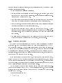
3.2.2 System's Architecture
The system coded for calibration was meant to verify the algorithm described
in section 2.5 and was specifying further the three main classes of the NOMAN
communication package. A more detailed class diagram can be found in Figure 11.
There is one main server (specifying ServerBase ), in charge of sending requests
to its clients and organize the system, as well as for the computation of the 3D
transformation. There are also two clients (specifying clientBase ), one dedicated to
the robot and the other one to the cameras.
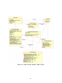
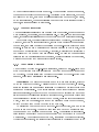
As the state diagram shows in Figure 12, the server mostly goes through a loop,
asking the robot to go to a specic position in the robot's frame rst, then asking
the cameras for their estimation of the position of the robot arm. When all points
have been visited, the server neglects the useless points for calibration and computes
the 3D transformation matrix from the remaining points.
The 3D points to which the robot is driven are computed from parameters written in the conguration le of NOMAN (more details in section E). When the server
starts, it reads those arguments and computes the 3D box inside of which the calibration has to be done.
Those arguments are set as :
• Xmin , Xmax ,
20
Figure 11: Specic Implementation Class Diagram
21
• Ymin , Ymax ,
• Zmin , Zmax ,
• d.
The variable d represents the distance between two points, so that the server
will compute a 3D grid inside the box and move the robot to every position at an
intersection of the grid. Therefore to avoid errors, preferably use dimensions that
set the gap to a multiple of d.
The transition between two states, on a UML Diagram is represented as :
[ <Event> ] [ '[' <Security check> ']' ] [ '/' <Response> ].
where the braces introduce an optional argument.
At least one of those three elements is required. Additionally, by personal decision, signs in capital letters represent communication between dierent elements of
the NOMAN architecture. Consider the following example:
[No more points required] / CALIBRATION_FINISHED.
It means that whenever the server gets the opportunity to follow this branch, it
will check if there are more points required for calibration. If not, it will follow this
transition and output a signal "CALIBRATION_FINISHED" (to all clients).
One may wonder whether the server or the cameras' client should handle the
detection of the robot arm. After a while, it seems obvious that as the cameras'
client is having access to the hardware information and internal calibration of the
cameras, it is much more ecient to conduct image treatment or feature extraction
on the cameras' client. This also avoid the transfer of the images over the network.
The calculation of the transformation matrix, as we saw it in section 2.5.2, is
done in an iterative way. Initially all the valid points are used, then as the rst
transformation matrix is computed, the server checks if there are points that are
absurd. An absurd point could mainly be coming from an error from the cameras'
client when estimating the 3D position, either due to noise not ltered or a person
moving in the eld of view of the cameras, perturbing the action of the lter. The
iterations are stopped when the furthest point for calibration is under a specied
threshold (see 2.5.4 for more details).
There is one main dierence between my implementation and the ServerBase
generalization, in term of functionality. It is due to an early error in the conception
of the system. As it was pointed out to me later, a server should "serve". It
would have been more logic to provide a server for the robot and a server for the
cameras. The calculation unit for the calibration would then have been carried
out by a client connecting both servers. The problem arises from the fact that a
22
Figure 12: TestServerCalibration State Diagram. A small description of the UML
norm can be found in section 3.2.2.
23
server in NOMAN is only able to send messages by pushing the same request to all
clientHandlers. Consequently, I had to create a few more tactics to avoid that the
cameras were asked to perform a robot motion, for example. To avoid such things,
when connecting the server, each client is telling its type (camera or robot), allowing
the clientHandler to be specic to this client. The clientHandler is also modied to
trash inaccurate messages for its client.
3.3
Robot's Client
3.3.1 KUKA's Script and Language
The script language provided by KUKA is highly restricted. It contains both functions to be called for moving the robot, as well as the required structural elements
(loops, boolean assertions, switch over integer values). Additionally, a set of thirteen functions are available to roughly deal with any communication process. Those
functions allow opening and closing of a connection, reading and automatic parsing
of the data in the XML received, as well as writing of data in the XML sent.
The script was kept simple by necessity. It consists of a loop, connecting to the
robot's client, then alternatively, awaiting a message containing a position and moving the robot there, then sending an acknowledgment in the form of an incremented
counter. The script was kept free of any error handling, not supported by the scripting language. For further details, please refer to the Programming instruction [14]
and the Ethernet XML documentation [15] of the KUKA robot.
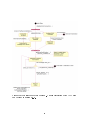
3.3.2 General Presentation
The most important part of the robot's client is its initialization, described in the
state diagram in Figure 13. It requires a heavy communication between dierent
elements of the architecture. It has to simultaneously contact the calibration server
and await a connection of the KUKA robot script.
Once this step is performed, the client sends positions to the the robot, waits
for the end of the motion and transfers the information to the server. It builds the
XML structure of the messages and parses the received messages using an additional
library.
3.3.3 tinyXML Parser
When reading the documentation [15] of the KUKA arm it seems that the use
of XML messages can only improve the safety of the communication (well-formed
structures) and broadens the range of possible applications. Thus an additional
package was installed to exploit at their best those opportunities. Unfortunately,
the KUKA controller, running on Windows, does not support the printed version of
24
Figure 13: TestClientRobot State Diagram. A small description of the UML norm
can be found in section 3.2.2.
25
the XML written by tinyXML. There are several reasons: the KUKA parser does not
support indentation or additional spaces and is incompatible with the line breaker
character under Unix systems.
Modifying those parameters in the library was making it useless (as it required
reprogramming the printing function for a complete document, using sub-nodes
over-dened printing functions). The library tinyXML was consequently only used
for reading the incoming messages from the KUKA controller. As the incoming and
output structure of a XML le in the KUKA controller have to be, anyway, strictly
static, a simple stream operation was sucient for sending the proper data.
3.3.4 Problems
The problems faced with the robot are not linked to the code of the client. The
controller however, happens to have unexpected behavior. The numerous workspace
protections (described in section D) are sometimes making the controller have trouble nding a proper way to move the robot from one point to the other. It often
happens that a point is out of reach: those errors can not be handled, as the script
simply crashes with no further notice. This forces you to modify your calibration
box (see section 3.2.2) and sometimes your home position to a more accessible area.
One last erratic aspect of the KUKA controller was its behavior when sending
the XML le. It happened that the XML structure received was short of the rst
half of the XML. I am not certain this error was caused by the controller, although
once a temporizing of half a second was added in the loop, at the end of each motion,
this problem disappeared. To look after this problem, the robot's client is always
outputting in the terminal windows the received XML message.
3.4
Cameras' Client
3.4.1 Frame Grabber
As described earlier (section 3.1.2) the cameras were provided with an open source
software, showing examples and explaining how to use a frame grabber in own
applications. The frame grabber still required a few tweaks to work properly.
The problem arose from the fact that the softwares were meant to be used for
the initial camera (STH device) and had almost not been modied for the STOC
device. Unfortunately, the STOC cameras have additional parameters stored in the
hardware and perform operations that require the frame grabber to be acquired
dierently. There are a few parameters that can be modied manually, in particular
the processing mode on the chip can take several values, as well as the color algorithm
used (more details in section A).
Mainly, you should know that some parameters, essentially those that are stored
on the chip, need to be dened previously to the acquisition of images and require
26
to be set before starting the frame grabber. When changing one such parameter,
the user needs to reset the frame grabber. Concerning other parameters, which are
not related to the chip, such as an additional rectication on computer, the colors,
or the color algorithm, the user necessarily has to set them after starting the frame
grabber, as those are erased at every reset.
3.4.2 General Presentation
The cameras' client is slightly more complex than the robot's. It has to deal with
more messages, but remains, in the overall simple. At rst, same as for the robot's
client, it consists of initializations of the hardware and communication structures.
Once this is done, the client will await requests from the server. As described in
Figure 14, every time a request is received, it attempts to capture both images from
the cameras, then tries to extract the position of the end-eector point from those
pictures. In case the arm manipulator was properly detected in both images, it will
produce a 3D reconstruction of the point. Otherwise, it will create an invalid frame
but will anyway try to send back some information. In case the communication
fails between the cameras' client and the server, the server will also have a security,
marking the expected (but never received) frame invalid.
3.4.3 Arm Position Detection
One advantage of doing "eye-to-hand" calibration, instead of "eye-in-hand" is to
avoid the extraction of images features from an object (for example a chess board
on the table). There is still a need to extract the position of the end-eector point
in space, which is not necessarily a simpler problem.
Possibilities The rst idea coming in mind was to use a simple light, attached
on the end eector of the robot. This light would be very easy to extract, in particular if the environment was darkened articially (by turning o the light tubes when
performing a calibration). Even if this solution was ecient (absence of parasite
lights in particular), it would have too much impact on the environment and would
limit the uses of the calibration algorithm for future works. For example doing a real
time calibration by storing in memory the 3D points, while the robot is performing
a task, would not be possible, even though the algorithm could be kept the same,
as such a device would be hard to detect in the work eld.
An alternative was to apply on the robot end-eector a pattern, such as a small
symbol or set of symbols. Those symbols would then have to be extracted from
the images and a 3D position computed from them. This solution is generally applied [11] and small black or red dots are printed on a at surface on the robot
manipulator. The requirements are very high, considering the feature extraction.
Whichever the pattern is, the feature extractor requires to be resistant to any ane
27
Figure 14: TestClientCameras State Diagram. A small description of the UML
norm can be found in section 3.2.2.
28
transformation, as well as partial occlusion, light conditions and sudden lighting
changes. Besides, it was dicult to stick a large piece of paper on the robot manipulator, or the Barret Hand (which was meant to be covered by tactile sensors for
posterior control of the grasping abilities).
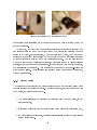
Solution I opted for a blinking electroluminescent diode. It is a rather easy
object to detect: very resistant to changes in the lighting conditions . A diode can be
as big as a pinhead, but a bigger one was chosen (5 mm), for more ease in detection.
The cameras were not inuenced by the light tubes from the laboratory, ickering
at 100 Hz.
The rst attempt was to use a simple, self blinking, diode. The frequencies
oered by such diodes range from 1 to 2.5 Hz, which was too low for a fast tracking
at a video rate. Consequently the blinking was provided by a simple relaxation
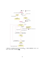
oscillator, using an integrated component: NE555 timer, in an astable mode. The
circuit schema is provided in Figure 15. Using a proper set of resistors and capacities,
both the loading time (diode o) and discharge time (diode lit) could be precisely
dened. It was decided to pick a blinking frequency of 15 Hz, with both phases
equal in time (the ratio is as close as possible from one).
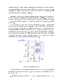
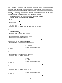
Figure 15: Electronic schema
Without giving too many useless details about the NE555 device, the tensions'
evolutions are described in Figure 16, and the steps in the functioning can be
summed up to:
1. Initially the capacity C1 is empty (Vc = 0), NE555 is not triggered and Vout = 0,
29
Figure 16: Voltages
2. the capacity C1 is loaded through R1 and R2 , up to the point where it reaches
2
V
, NE555 is then triggered and Vout = Valim ,
3 alim
3. the capacity C1 discharges itself through R2 , until when, at t1 , it reaches 31 Valim
and NE555 is reset, Vout = 0,
4. the circuit goes back to step 2 for the time t2 .
The law for the voltage when discharging is given by:
−t
Vc (t) = Valim e R2 C1
And when loading:
−t
2 (R +R
)C
Vc (t) = Valim 1 − e 1 2 1
3
Therefore, the times t1 and t2 (see Figure 16) are:
t1 = ln (2) R2 C1
t2 = ln (2) (R1 + R2 ) C1
and consequently:
30
T = t1 + t2 = ln (2) (R1 + 2R2 ) C1
1
1
f= =
T
ln (2) (R1 + 2R2 ) C1
R2
t2
=1−
α=
T
(R1 + 2R2 )
Considering the price of the components and the available values, the choice was
oriented so that f = 15Hz, and α ' 0.5, which would mean that t1 ' t2 .
f=
1
= 15Hz
ln (2) (1.69 ×
+ 2 × 21 × 103 ) × 2.2 × 10−6
21 × 103
' 0.52
α=1−
(1.69 × 103 + 2 × 21 × 103 )
103
Three diodes were also chosen with a wavelength of 605 nm (orange), 571 nm
(green) and 470 nm (blue), as close as possible from the cameras best response to
illumination (the cameras' response can be found in section C). In the overall with
cameras working at 30 fps (a common used rate), ideally if the rst image showed
a dark diode, every other image would contain a lit diode. This would make it
very easy and robust to detect. A small metallic box was designed to contain a 9V
battery, a switch, the electronic circuit and the diode (the strip board layout may
be found in section B).
As the images were slightly blurry when using rectication, (for comparisons between cameras' modes, go to section A) and as it was thought this could damage the
eciency of any feature extractor, the frame grabber was used with no rectication,
neither on the chip, nor on the computer. Once the diode is detected in both views,
it is still time to rectify its position depending on the lenses deformation, as the
cameras were calibrated in factory and make the rectication matrices available for
download from the hardware.
As there was not any particular use of the colors for detecting the diode, the
pictures were restricted to Black & White, the increase of the video capture frame
rate being a nice side eect. A small metallic box, presented in Figure 17 was built
to contain the electronic circuit, the battery and the diode, avoiding power supply
wires.
Problems A strange problem appears when turning on the diode: the blinking
is irregular and chaotic. It was rst suspected to be due to the loading time for the
capacity used in the circuit but the transition time was too long, about 10 sec. The
reason probably comes from the time required for the components to reach a stable
31
Figure 17: Metallic box with blinking diode
temperature (this transition time does not appear when only switching o and on
again the blinker).
As expected, the diode and cameras frequencies are not perfectly adjusted and
one shall not rely too much on the time stamp of a picture for deciding upon the
status of the diode. In our situation, we were not limited by time, but we were not
storing in memory the last position of the diode in the image (requiring therefore
to treat complete images for every new calibration point). The cameras store in
memory a set of twenty consecutive pictures, which is far enough to bring satisfying
results, once the images have been ltered. It was measured that on thirty pictures,
the frequencies were aligned. This means that there is one extra half-period for
every fteen periods. Those results were obtained using a camera in monochrome,
with no rectication.
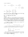
3.4.4 Filter Applied
The lter used for extracting the diode position works with the strong assumption
that its environment should be static. The lter executes, for every picture and for
every pixel, the steps described next.
• The lter calculates the dierence of intensity with the same pixel, in the
previous picture,
• it applies a threshold on the absolute value of the dierence of intensity and,
• if a pixel passes the threshold, the result pixel (initially at zero) at this position
will be incremented.
32
• Afterwards, a mask is applied by convolution. The mask used here was :
DimF ilter
 ←−−−−−−→ 
1
...
1





.
.
.

 ..
.
.
.
.






1
...
1
and then, the lter applies another threshold on the result.
• Finally, the mean of all pixels that passed the last condition is computed.
Typically, the diode is represented as a small area, lled with points alternatively
bright and dark. The rst threshold is there for avoiding slight luminosity changes
and the second one to erase noise such as people walking through. The size of the
lter is mostly depending on the working distance and the intensity of the result
pixels should be set at almost 100% as the diode's pixels should all contribute at
every frame.
If n(x, y) is the number of pixels that passed the lter of dimension D applied
for a specic (x, y) in the picture, the threshold at P %, P ∈ [0, 100], for a set of m
pictures is dened as 100 × n(x, y) > D2 × m × P .
There is a total of two safety measures, to insure the calibration will be of good
quality. First, when a 3D reconstruction can not be performed, the point is labeled
as invalid for the calibration process. Also, the system gets rid of absurd points
(described in section 3.2.2) in an iterative way.
3.4.5 Problems
I encountered a few problems with this lter in its early versions. As the lter size
was constant, it happened that when working too far from the cameras, the diode
was considered as noise. This last version showed to be quite versatile and adaptable.
One could still imagine situations where another diode in the background (monitor
in stand by, hard disk being accessed) could interfere strongly with the lter. Once
again, the complete algorithm has other securities and the risk would rather be to
lack calibration points and perform a low quality transformation matrix than not
detecting the diode at all.
3.5
Summary
This communication works ne if you neglect a few cases where a message is lost
and the whole calibration needs to be rebooted (every element awaiting a message
from another part of the system).
33
To conclude on the implementation, I would say that NOMAN was a logic choice
given the information I had. It was providing a nice wrapper class, allowing to dene
messages by type and making the whole communication architecture much simpler.
It was also giving access to precoded function for matrices, such as invert, pseudoinvert and singular value decomposition. This was my rst project using C/C++
and relying on already coded les helped a lot getting a quick grasp on the language.
Unfortunately, I was told lately that most of the package was deprecated or left
unattended. I could anyway help transfer some of my work to another system, using
a CORBA architecture.
34
4 Evaluation
4.1
Filter Parameters
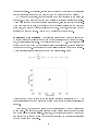
I present here successive steps in the extraction of the diode position, the results
at each step and the inuence of dierent parameters. You may recall the dierent
steps in the section 3.4.4.
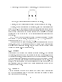
Images Those are the rst pictures and give a simple view of the raw material
(see Figure 18) from which the diode needs to be extracted. Although the pictures
in Figure 19 seem similar and the eye can not easily make the dierence, we will see
further that the dierence of luminosity is noticeable. Those pictures represent the
pixels values, with:
p(x, y) = I(x, y, t0 ),
where p is the pixel value at the position (x, y), and I(x, y, t) is the luminosity
intensity for the pixel (x, y) in the picture captured at t.
Figure 18: Left view of the cameras
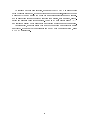
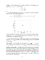
Luminosity derivative The results in the histogram (see Figure 20 are output
by taking the absolute value of the subtraction of one image from the next one. It
is a simple way to do the discretization of the derivative of the luminosity in time
and to implement it. Those pictures represent treatment done on the pixels values,
with:
p(x, y) = |I(x, y, t0 + 1) − I(x, y, t0 )|.
When applying successive thresholds (see Figure 21), one can see that with
a threshold high enough, this single step would be sucient to detect the diode's
position. However this experiment was conducting with no strong noise, nor lighting
35
Figure 19: Two successive images from the left camera. Although it might not be
visible, in the left picture, the diode is o and it is lit up in the right one.
Figure 20: Histogram of pixels' luminosity dierence, a pixel's intensity ranges between 0 and 255.
Figure 21: Luminosity dierence between two images, thresholded at T units per
pixel, with T ∈ {4, 10, 20, 30, 50, 70}.
36
condition changes. Additionally, it is dicult to decide on where to set the threshold:
are very lit points those from the diode or from a moving edge in the picture?
To be sure of the result, one could implement a segmentation of the areas for
example. It would probably provide good results if excluding invalid estimations.
This would shorten the whole detection process a lot, allowing fast time detection.
Even with only two images, the chances to get the correct position for the diode are
quite high, and could be done at a frequency of 15Hz. However, our system did not
require to be fast but robust. This is why we performed the next step.
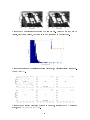
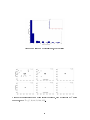
Summing up a set of images The results in Figure 22 and Figure 23 are output
by incrementing each pixel for each image when it was lit enough to pass the threshold, but regardless of its value. The threshold used was T = 20. This threshold was
chosen as it got rid of 90% of the useless points (cameras' noise), without shrinking
the area of the diode. This is probably the smallest threshold that can be applied.
Those pictures represent treatment done on the pixels values, with:
p(x, y) =
tX
0 +19
(|I(x, y, t + 1) − I(x, y, t)| > 20) .
t=t0
Figure 22: Sum for 20 images of the luminosity dierence thresholded at T = 20:
the result is scaled so that a pixel with a value of 20 (maximal value) is represented
in black.
Once again, you can see in Figure 24 that thresholding at 15 or 18 units would
be sucient. And once again, a simple error of a few units would bring a lot of noise
and a high risk of detection failure. Moreover, the capture time has now been about
one second (20 images at a rate of 30 frames per second) so that fast applications
have no use for such a process.
37
Figure 23: Histogram of resulting pixels' values after summing up the dierence of
luminosity in 20 images, thresholded at T = 20.
Figure 24: Results of summed up luminosity dierence, with a threshold at T units
per pixel, with T ∈ {1, 2, 5, 10, 15, 18}.
38
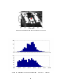
Filtering After thresholding, a simple lter was applied by convolution. It was
chosen with DimF ilter = 3 which means


1 1 1


F = 1 1 1.
1 1 1
.
The result is represented in Figure 25. The picture in Figure 26 represents
treatment done on the pixels values, with:
p(x, y) =
x+1
X
y+1
X
x0 =x−1 y 0 =y−1
"t +19
0
X
#
(|I(x0 , y 0 , t + 1) − I(x0 , y 0 , t)| > 20) .
t=t0
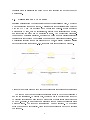
Figure 25: Result, when ltering the sum for 20 images of the luminosity dierence
thresholded at T = 20: the result is scaled so that a pixel with a value of 180
(maximal value) is represented in black.
As you can see in Figure 27, the threshold can be set in a much wider range (typically from 20 to 150). Apart from being a useless exploit, it shows the robustness
of the system.
Final results Once the ltering and thresholding at 80% (i.e.
T = 144) were
done, the algorithm simply takes the mean value. The result is output in Figure 28.
Stability considerations It was also tried to record a sequence of 1000 pictures,
extracting for each set of 20 consecutive pictures the diode's position. By looking
at the Figure 29, one can see the results are highly satisfactory (especially when
considering that someone was sometimes moving in the background). The estimation
of the diode position is included in a space of 5.10−3 pixels × 5.10−3 pixels. As you
can see in Figure 30, a light noise was even provided by a person making small
movements in the background.
39
Figure 26: Histogram of pixels' value, post ltering
Figure 27: Results ltered sum of luminosity dierence, with a threshold at T units
per pixel, with T ∈ {5, 10, 20, 50, 100, 150}.
40
Figure 28: Final estimation for the position of the diode
Figure 29: Histogram of the diode position in Y (top) and X (bottom)
41
Figure 30: Examples of small motions in the backgrounds, the left image shows the
view of the camera and the right image is the dierence of luminosity between this
image and the next one.
Discussion As one can see here, maybe the rst step in the process would be
quite sucient to detect a rather precise position. However, this was not robust at
all. The whole process consists of ltering the data both in time and space, giving it
resistance to both noise due to people moving, or luminosity changes (noise in space
but not in time, i.e. very visible in a few pictures at a localized spot, but negligible
on the whole set of picture) and to noise due to the CCD array of the cameras (noise
in time but not in space, i.e. present in every pictures, but not at the same place).
When conducting the experiments, a few details were noticed. The angle of
inclination of the manipulator and therefore of the diode is primordial for a proper
detection. The diode emits light in a cone with an opening of about 20◦ and even
the eye can not see the light under that angle. When the diode is strictly in the
axis of the cameras, there can be a halo appearing around the center of the diode.
Also, since the system was created some months ago, the battery seems to be not
as ecient as it used to be, and the low current aects the amount of emitted light.
Depending on the lighting conditions, and unless the lter's parameters are automatically optimized, the user needs to set some values manually. To perform this
task, the user can decide to plot information about the graphic values. All this
needs to be done in the code, and to recompile afterwards. The verbose argument,
when calling the method takeStereoPicture in TestClientCameras.cc shall be set to
two or superior, the program will then output a set of pictures, as well as preliminary results from the features extraction. This feedback should help to dene the
thresholds that will be applied, at the successive steps of the ltering process.
The last parameter which may be discussed is the size of the set of pictures used
for extracting the arm position. Twenty pictures were used. The only reason was
that the time for capture was inferior to one second and the results were satisfying.
Less pictures could probably give a good result also.
42
4.2
Position Errors
We have seen that the precision on the detection of diode was hardly a problem when
done in good conditions. Now we can consider the precision of the least square error
algorithm (described in section 2.5). It was tested on several sets of points. There
are three sets of points used for calibration, with a dierent amount of points and
also a set of random points, used for testing the precision of the transformation
matrix. All distances are in mm. The cube inside of which they were all taken is of
coordinates [-100, 100] x [500, 700] x [400, 600].
Figure 31: Reconstructed setup in 3D, showing cameras' and robot's frames origins,
as well as the 3D box inside of which the points will be taken for calibration.
Small set This set is made of 8 points, organized in a rectangular grid in 3D, with
a distance of 200 mm between points in every direction.
Out of those 8 points, 7 were used for estimating the transformation matrix
(i.e. one point was either not detected or absurd for calibration). The resulting
calibration matrix (from cameras' frame to robot's frame) is :


−3.72759 −0.0730479 −0.197893 74.0506


0.0172192 −0.295156 −4.68294 1316.84
0.0677304 −3.69473
0.659815 409.383
Medium set This set is made of 27 points, organized in a rectangular grid in 3D,
with a distance of 100 mm between points in every direction. Out of those 27 points,
26 were used for estimating the transformation matrix (i.e. one point was either not
detected or absurd for calibration). The resulting calibration matrix (from cameras'
frame to robot's frame) is :
43


−3.72067 −0.06236 −0.167075 68.2836


0.0220495 −0.195601 −4.71205 1318.67
0.0719473 −3.71624 0.617452 416.388
Large set This set is made of 125 points, organized in a rectangular grid in 3D,
with a distance of 50 mm between points in every direction. Out of those 125 points,
only 121 were used for estimating the transformation matrix (i.e. four points were
either not detected or absurd for calibration). The resulting calibration matrix (from
cameras' frame to robot's frame) is :


−3.71679 −0.0660879 −0.173719 69.28


 0.045216 −0.161896 −4.71071 1318.87
0.0681365 −3.74337
0.64431 411.814
Setups comparison The rst easy measure we can do is on the points that were
used for calibration. In those three sets, the mean of the displacement error should
be zero (as the least square error algorithm outputs a solution with no bias). The
interest in the comparison lays in the standard deviation. In Figure 32, one can see
the reconstructed setup and the error for each point.
Figure 32: 3D representation of the calibration points and their error, for density
comparison (successively 8, 27 and 125 points), according to the axis of projection
(in the robot's frame).
44
Error on the calibration sets, using a 3D reconstruction In the Figure 33
the distance error between a point used for calibration in the robot's frame and
its equivalent in the cameras' frame (once reconstructed and translated back into
the robot's frame) is measured. An histogram is being plot: this allows an easy
comparison of the variance on the error for calibration points, depending on the
amount of points used.
Error on the test set, using three dierent calibrations In the Figure 34,
similarly to the previous gure, the distance error is measured and an histogram is
being plot. This error is however measured on the set of 200 test points. This allows
an easy comparison, not only of the variance, but also on the potential bias and the
inuence of the number of points used for calibration.
Error on the test set, using a 3D representation The Figure 35 is just meant
to show how the 3D random points from the test set were located and what the error
with their estimated position is. This is only for the reader to get at a glance what
the test set is like. The calibration used for performing this reconstruction has been
computed using the set of 125 points.
Discussion In Table 1 some mathematical values are presented, for an easier
comparison between the dierent calibration sets.
Npoints
8
27
125
|X| (mm)
µ
σ
|Y | (mm)
µ
σ
|Z| (mm)
µ
σ
d (mm)
µ
σ
1.487 1.071 7.977 8.484 1.845 1.527 8.652 8.356
1.353 1.049 7.511 8.148 1.786 1.465 8.186 8.002
1.280 0.986 7.332 8.23 1.602 1.478 7.962 8.090
Table 1: Comparative table of the displacement error made on the test set (200
points), using the three successive calibrations. |X|, |Y | and |Z| represent the absolute value of the distance projected according to the axis in the robot's frame, d
is the distance in space, when transforming a point from the cameras' frame to the
robot's frame.
The rst impression pointing up is that even with a low number of points used
for calibration, the result is satisfying. As one could see in the histograms, the
test set has quite a large error. That explains why one should not be shocked by
an error with a mean of eight millimeters. It is much more interesting to compare
the dierence between the mean among dierent calibrations: whether you use 125
points or only 8 points, the loss in precision is smaller than one millimeter.
Also, the main part for displacement error is projected on the Y axis of the robot,
which is, in the conguration I used, very close from the X axis of the cameras: the
45
Figure 33: Histograms of the displacement's error on the three calibration sets
(successively 8, 27 and 125 points), according to the axis of projection (in the robot's
frame).
46
Figure 34: Histograms of the displacement's error on the test set (containing 200
points), using the three dierent calibration matrices (successively computed with
8, 27 and 125 points), according to the axis of projection (in the robot's frame).
47
Figure 35: Representation in 3D of the test points in the robot's frame and the
cameras' frame, with the displacement error, according to the calibration computed
with the large set of 125 points.
48
error mostly comes from imprecision in the depth estimation (as the error in the
cameras has more impact on the depth, due to projective properties).
Eventually, one can notice that the main advantage of using a large set of calibration point is to reduce the bias (which is minimized directly by the least-square
algorithm), but it has little eect on improving the standard deviation. The improvements (less than one millimeter) are anyway low, considering the amount of
additional time required (I remind you most of the time spent on calibration is spent
on the robot's motion). Be careful, however, to have a sucient amount of points
to produce a viable transformation matrix (6 points are advisable); if you happen
to select a calibration box where most of the points are outside the eld of view of
the cameras, the resulting transformation matrix would be worthless.
49
50
5 Conclusion
When addressing the issue of using visual information to control a robotic arm, a
calibration is required. To estimate the position and orientation of the cameras
relatively to the robot, the robotic arm end-eector point has to be detected at
successive locations in space. This thesis provides simultaneously an electronic device, meant to be attached to the end-eector, for tracking a point in space, and an
associated video lter, that makes the device easy to detect. It also contains the
implementation of a simple algorithm for computing a 3D transformation matrix.
The complete process runs almost autonomously and can be executed on a network
interface, specic to CVAP/CAS. Both the sensors and the actuators classes could
be easily modied in case the equipment used was changing. The resulting calibration between the cameras and the robot arm is precise to the extend of a few
millimeters.
By the time my work reached this point, a Barrett Hand has been mounted on
the KUKA arm. The small electronic device (previously set into a metallic box)
has been inserted in the free space on the back of one of the ngers (the Barrett
Hand can be seen in Figure 1). When performing calibration, the hand is set in a
x position, while the arm calibrates itself relatively to the cameras.
Moreover, the Barrett Hand is equipped with tactile sensors. Also, a humanoid
head (a replica from the head of the ARMAR-III robot) is looking at the setup. To
the setup already installed (a CORBA architecture with servers for every sensor), a
CORBA server wrapping the KUKA arm was added.
So any user can design a client adapted to his own application, whether it is
estimation of grasping points and simple grasp attempts or imitation of human
grasp behavior. However, due to the restriction on the KUKA software, automatic
control of the position of the hand when grasping is not yet available. This makes
applications such as pushing an object on the table or holding on to slippery objects
impossible.
Focusing further on the KUKA arm and the control of the hand, it is very likely
that the next step will be to create a system allowing visual servoing and real-time
control, using a dierent set of sources for the KUKA arm. This will allow a control
closer from what a human can do, smoother and very precise on a local, relative
scale.
The electronic device provided in this project for calibration might not be sufcient and, either more diodes would need to be installed, or the position of the
arm would need to be detected using completely dierent features. The KUKA arm
showed to have short sighted applications but was very reliable. I can only hope the
new source code package will broaden those applications while remaining reliable.
51
52
6 Bibliography
References
[1] PACO-PLUS, ocial website:
http://www.paco-plus.org/
[2] Asfour T., Regenstein K., Azad P., Schroder J., Bierbaum A., Vahrenkamp N.
and Dillmann, R. ARMAR-III: An Integrated Humanoid Platform for SensoryMotor Control, Humanoid Robots, 2006 6th IEEE-RAS International Conference
[3] Andrew T. Miller and Peter K. Allen. GraspIt!: A Versatile Simulator for Grasp
Analysis
[4] S. Hutchinson, G. Hager and P. Corke. A tutorial on visual servo control, IEEE
Transactions on Robotics and Automation, October 1996.
http://www.cs.jhu.edu/~hager/Public/Publications/TutorialTRA96.
pdf
[5] F. Chaumette and E. Malis. 2 1/2 D visual servoing: a possible solution to
improve image-based and position-based visual servoings. In IEEE Int. Conf.
on Robotics and Automation, ICRA'00.
http://ieeexplore.ieee.org/iel4/70/16447/00760345.pdf?arnumber=
760345
[6] Gregory D. Hager, Wen-Chung Chang and A. S. Morse, Robot Hand-Eye Coordination Based on Stereo Vision, 1995.
[7] Tsai R.Y. and Lenz R.K. Real Time Versatile Robotics Hand/Eye Calibration
using 3D Machine Vision, Robotics and Automation, 1988.
[8] Yiu Cheung Shiu and Shaheen Ahmad. Calibration of Wrist-Mounted Robotic
Sensors by Solving Homogeneous Transform Equations of the Form AX = XB ,
February 1989.
[9] D. DeMenthon and L.S. Davis. Model-Based Object Pose in 25 Lines of Code,
International Journal of Computer Vision, June 1995.
[10] PACO-Plus Wiki, restricted access.
http://www.nada.kth.se/cas/local-information/pacoplus/pacowiki/
[11] Christian Wengert, Computer Vision Laboratory, Swiss Federal Institude of
Technology Zurich. Matlab Toolbox for Hand-in-Eye Calibration.
http://www.vision.ee.ethz.ch/~cwengert/calibration_toolbox.php
53
[12] Videre Design, Menlo Park, CA. STH-DCSG-VAR/-C Stereo Head, User's
Manual. Issued 06.2007, Version ?
http://www.videredesign.com/docs/sthdcsg-var.pdf
[13] Videre Design, Menlo Park, CA. [...] STOC, Stereo head, User Manual 1.3.
Issued 05.2007, Version 1.3.
http://www.videredesign.com/docs/stoc-1.3.pdf
[14] Kuka Roboter GmbH, Augsburg. KUKA System Software 7.0, Operating and
Programming Instructions for Systems Integrators. Issued 11.08.2006, Version
1.2.
[15] Kuka Roboter GmbH, Augsburg. KUKA.Ethernet KRL XML 1.1 For KUKA
System Software (KSS) 5.x. Issued 23.11.2006, Version 0.1.
54
A Cameras' Frame Grabber Parameters
The processing mode on the chip can take several values, as well as the color algorithm use.
• PROC_MODE_OFF
• PROC_MODE_NONE
• PROC_MODE_TEST
• PROC_MODE_RECTIFIED
• PROC_MODE_DISPARITY
• PROC_MODE_DISPARITY_RAW
And the color algorithm :
• COLOR_ALG_FAST,
• COLOR_ALG_BEST.
Here are a few pictures, depending on the parameters. Those pictures were captured using the smallv application provided with the cameras device. They should
help you decide upon the parameters you want to use for your own application.
More information can be found on the PACO-Wiki (restricted access) [10].
First, you need to decide whether you want the STOC device to compute the
3D map on the chip, in such a case, you need to activate the processing on chip
and ask for a disparity map. I was rather interested by comparing the automatic
rectication on chip with the one computed by the computer, you can observe the
picture without rectication in Figure 36 and the rectied ones in 37.
Figure 36: Original, not rectied picture, extracted from the STOC device
The "BEST" algorithm is providing a very smooth and precise image, whereas
the "FAST" algorithm has some trouble with interlaced lines, causing a slight shift
55
Figure 37: Comparison of rectication on chip (left picture) and rectication on
computer (right picture) for a picture extracted from the STOC device
Figure 38: Comparisons of color algorithms, Fast (left picture) and Best (right
picture)
56
from one line to the next. This makes any edge very blurry. Those parameters
probably only play a role when performing 3D reconstruction directly on the chip,
as this would inuence the performances of the cameras (the number of frames per
second). In our case, we didn't have to worry about frequency when it came only
to lm the scene. Therefore the "BEST" algorithm was used.
I will here present how to get the frame Grabber, in details:
First you need to check hardware colors availability.
int r ;
r = Fl : : v i s u a l (FL_RGB8) ;
i f ( r == 0){
r = Fl : : v i s u a l (FL_RGB) ;
i f ( r == 0){
DebugCERR( 3 0 ) << "Can ' t run i n f u l l − c o l o r mode\n " ;
}
}
Initialize pointers. . .
svsVideoImages ∗ v i d e o O b j e c t = NULL;
s v s S t e r e o I m a g e ∗ s i = NULL;
svsAcquireImages ∗ s o u r c e O b j e c t = NULL;
v i d e o O b j e c t = getVideoObject ( ) ;
Dene the parameters that will be loaded on the chip of the cameras. All those steps must be
done BEFORE any frame grabber is initialized.
i f ( videoObject −> SetFrameDiv ( frameDiv ) ) {
DebugCERR( 3 0 ) << "Frame d i v i s i o n s e t to "
<< frameDiv
<<" on VideoObject . \ n " ;
} else{
DebugCERR( 3 0 ) << "Can ' t s e t frame d i v i s i o n on v i d e o O b j e c t . \ n " ;
}
i f ( videoObject −>S e t S i z e ( width , heigh ) ) {
DebugCERR( 3 0 ) << "Frame s i z e = "
<< width
<<"∗"
<< heigh
<<" on VideoObject . \ n " ;
} else {
DebugCERR( 3 0 ) << "Can ' t s e t frame s i z e on v i d e o O b j e c t . \ n " ;
}
i f ( videoObject −>SetRate ( r a t e ) ) {
DebugCERR( 3 0 ) << "Frame r a t e s e t to "
<< r a t e
<<" on VideoObject . \ n " ;
} else {
DebugCERR( 3 0 ) << "Can ' t s e t frame r a t e on v i d e o O b j e c t . \ n " ;
57
}
For other available modes see svs.h or svsclass.h Here for example, we would be setting the
rectication on chip OFF (processingM ode = P ROC _M ODE _N ON E )
i f ( v i d e o O b j e c t && videoObject −>is_proc_capable ){
i f ( videoObject −>SetProcMode ( processingMode ) ) {
DebugCERR( 3 0 ) << " S e t t i n g STOC p r o c e s s i n g mode to "
<< processingMode
<< " on v i d e o O b j e c t . \ n " ;
} else{
DebugCERR( 3 0 ) << "Can ' t s e t p r o c e s s i n g mode on v i d e o O b j e c t . \ n " ;
}
}
Extract the actual mean of getting images, out of the videoSource, and open the frame grabber.
s o u r c e O b j e c t = ( svsAcquireImages ∗ ) v i d e o O b j e c t ;
i f ( sourceObject −>Open ( ) ) {
DebugCERR(20)<< "Opened frame grabber . \ n " ;
} else {
DebugCERR(20)<< "Can ' t open frame grabber . \ n " ;
w h i l e ( f l t k _ c h e c k ( ) ) {}
return f a l s e ;
}
When creating a frame grabber, any parameter that has been set previously is erased, therefore
we need to set them now (once opened):
i f ( videoObject −>S e t C o l o r ( c o l o r L e f t , c o l o r R i g h t ) ) {
DebugCERR( 3 0 ) << " C o l o r s parameters s e t on VideoObject . " ;
} else{
DebugCERR( 3 0 ) << "Can ' t s e t c o l o r s parameters on v i d e o O b j e c t " ;
}
Here it seems we need to redene rectication as false, but it doesn't give away any conrmation.. this function is very very weird.. but just look at what happen if you don't do it. I'm
thinking maybe SetRect() does not return true of false whether the rectication has been set, but
rather isRectied. Therefore, when setting rectication to false, it returns false if it worked (it does
return true when setting rectication to true). This is not coherent with other functions though !
i f ( videoObject −>SetRect ( r e c t i f i c a t i o n O n C o m p u t e r ) ) {
DebugCERR( 3 0 ) << " R e c t i f i c a t i o n on computer s e t to "
<< r e c t i f i c a t i o n O n C o m p u t e r
<<" on v i d e o O b j e c t . " ;
} else{
DebugCERR(30)<<"Can ' t s e t r e c t i f i c a t i o n parameter
on computer , on v i d e o O b j e c t " ;
}
For other algorithms, see svs.h or svsclass.h Algorithm Fast tends to create those "vibrating
edges" in images.
videoObject −>c o l o r _ a l g = c o l o r A l g o r i t h m ;
Only when all parameters have been dened, we can start the capture.
58
i f ( ! sourceObject −>S t a r t ( ) ) {
DebugCERR( 2 0 ) << "Can ' t s t a r t c o n t i n u o u s c a p t u r e . \ n " ;
w h i l e ( f l t k _ c h e c k ( ) ) {}
return f a l s e ;
}
return true ;
59
B Board Layout of the Electronic Circuit
The layout in Figure 39 is very close of the actual one I used for my system. The
× represent the points where the copper lines (on the back of the board) have to
be scratched out, to prevent electrical contact between the left and the right side of
the NE555 component.
Figure 39: Strip board layout
60
C Cameras' CCD Array Response
I hereby introduce some graphics extracted from the Videre manual from both the
STH [12] and the STOC [13] devices. Those are meant to justify the choice in
the diodes wavelength, considering the response of the cameras' CCD arrays (in
Figure 40) and the global transmittance of the cameras (in Figure 41.)
Figure 40: Imager Response - Color
Figure 41: Filter Transmittance
61
D KUKA Workspace Protection
To prevent damaging the environment through motion by the robot, or to restrict the
workspace, the users can dene protections in both Cartesian an axis-specic spaces.
Those protections can be either respected, or slightly violated. In both cases, the
controller will output a message and regarding if the envelope was violated or not,
requires the user to acknowledge the violation, to override protections, acknowledge
again the message and jog the robot back into its legal workspace. When running
a program, the controller does not check the motion in the user's protections space,
therefore any motion will happen until the robot actually runs out of its workspace;
the program will then stop.
There are so far four main protection workspaces dened :
• the wall,
• the table under the KUKA arm,
• the limit on angular values for the axis 5: hand mounting platform, motion
allowed between -90◦ and 90◦ .
• the limit on angular values for the axis 3: this axis could be dened as the
one between the forearm and the arm. The risk was, when having the hand's
ngers wide opened, to bump into the structure of the robot. The motions
allowed are between -119◦ (KUKA nominal value) and 130◦ .
To congure or override the workspace protections, you should:
• Set the mode to T 1,
• be in Expert mode,
• if you want to override a workspace violation, you need to acknowledge the
violation,
• select the menu Congure, Miscellaneous, Monitoring Workspace Protection
and Override or Conguration.
• if you want to override a workspace violation, you need to acknowledge the
override command, then you can jog the robot back in the valid workspace,
• if you want to dene or modify an existing workspace, you need to select
its type (Cartesian or axis) and number (names given should be as clear as
possible) and change the values written.
62
• A Cartesian workspace is dened as a cube, with an origin and 6 values (+X ,
−X , +Y , −Y , +Z , −Z ) applied to this origin. It may get confusing, so don't
hesitate to keep the origin of the cube at the origin of the robot coordinates
(0, 0, 0).
• An axis workspace is dened as the set of ranges the axis can reach. For every
axis, a couple of the form (θ, β) has to be dened. The protection number
1, although it is not used shows the minimum and maximum values one can
apply. Do not delete this protection.
• Eventually when all values have been entered, you need to select a mode.
OU T SIDE _ST OP is the usual one, meaning that the robot will remain
inside the cube,
• Do not forget to save thoroughly the changes made, as the controller will
otherwise erase them without even warning you.
We noticed on a reasonable speed setting (mode T 1 or T 2 at 100%) that the
violation of an axis workspace was of about 8◦ . You may consider 30 mm in Cartesian
if your workspace needs to be set that precisely. Think of this security margin.
You may decide upon the values used for the workspace protections by jogging
manually the robot to the maximal positions while observing the coordinates given
by the controller. This is done by selecting the menu Monitor, Robot Position then
decide between the Cartesian or axis mode.
63
E Noman Conguration File
!SERVERCONFIGS # DO NOT EDIT/REMOVE THIS LINE
# This is the conguration le for the servers/clients in the NOMAN system
# Each line that begins with a # is considered to be a comment line.
# Each line that does not t the format
# <servername(string)> <hostname(string)> <port(short) [whatever string]>
# is also ignored.
# WARNING! Do not use tabs, only use one or more spaces as separator!
# You can add an arbitrary number of arguments to the dierent
# servers by adding them after the third argument. When running the
# system a server will try to read this le and will look for a local
# copy rst and if no such le is found it will look in NOMAN/cong
# for a le. If still no cong le is found it will use the default port
# that was passed on to the server when instantiating it. An empty
# string with arguments will be passed to the server in this case.
# The clients will also read this le when using the function
# connect(), i.e without arguments.
GraspitArmServer localhost 5000
PumaArmServer moms-arm.nada.kth.se 5000
JR3Server dumbo.nada.kth.se 5003
[...]
TestServer localhost 5557 47 11 42
# The arguments for TestServerCalibration integers, organised in such a way:
# port xmin xmax ymin ymax zmin zmax distance
# So that the server will "meshgrid" a 3d box in the given cubic-coordinates,
# and go to every point on the 3d-grid (for calibration matters of course).
# The distance between each point of the grid should be equal to the param distance,
# therefore "xmax-xmin" should be a multiple of "distance".
#Distances in mm !!!
TestServerCalibration galaxy.nada.kth.se 6000 -100 100 500 700 400 600 200
[...]
64
TRITA-CSC-E 2008: 035
ISRN-KTH/CSC/E--08/035--SE
ISSN-1653-5715
www.kth.se